4_analyses_robust
Laura Botzet & Ruben Arslan
Robustness Analyses
Helper
source("0_helpers.R")##
## Attaching package: 'formr'## The following object is masked from 'package:rmarkdown':
##
## word_document##
## Attaching package: 'lubridate'## The following object is masked from 'package:base':
##
## date##
## Attaching package: 'broom.mixed'## The following object is masked from 'package:broom':
##
## tidyMCMC## Loading required package: carData## lattice theme set by effectsTheme()
## See ?effectsTheme for details.##
## Attaching package: 'data.table'## The following objects are masked from 'package:lubridate':
##
## hour, isoweek, mday, minute, month, quarter, second, wday, week, yday, year## The following objects are masked from 'package:formr':
##
## first, last## Loading required package: Matrix##
## Attaching package: 'lmerTest'## The following object is masked from 'package:lme4':
##
## lmer## The following object is masked from 'package:stats':
##
## step## Loading required package: usethis##
## Attaching package: 'psych'## The following objects are masked from 'package:ggplot2':
##
## %+%, alpha## This is lavaan 0.6-5## lavaan is BETA software! Please report any bugs.##
## Attaching package: 'lavaan'## The following object is masked from 'package:psych':
##
## cor2cov## Loading required package: lattice## Loading required package: survival## Loading required package: Formula##
## Attaching package: 'Hmisc'## The following object is masked from 'package:psych':
##
## describe## The following objects are masked from 'package:base':
##
## format.pval, units##
## Attaching package: 'tidyr'## The following objects are masked from 'package:Matrix':
##
## expand, pack, unpack##
## Attaching package: 'dplyr'## The following objects are masked from 'package:Hmisc':
##
## src, summarize## The following objects are masked from 'package:data.table':
##
## between, first, last## The following objects are masked from 'package:lubridate':
##
## intersect, setdiff, union## The following objects are masked from 'package:formr':
##
## first, last## The following objects are masked from 'package:stats':
##
## filter, lag## The following objects are masked from 'package:base':
##
## intersect, setdiff, setequal, union##
## Attaching package: 'codebook'## The following object is masked from 'package:psych':
##
## bfi## The following objects are masked from 'package:formr':
##
## aggregate_and_document_scale, asis_knit_child, expired, paste.knit_asis, rescue_attributes,
## reverse_labelled_values##
## Attaching package: 'effsize'## The following object is masked from 'package:psych':
##
## cohen.dopts_chunk$set(warning = FALSE)Load data
birthorder = readRDS("data/alldata_birthorder.rds")Data preparations
# For analyses we want to clean the dataset and get rid of all uninteresting data
birthorder = birthorder %>%
  filter(!is.na(pidlink)) %>% # no individuals who are only known from the pregnancy file
  filter(is.na(lifebirths) | lifebirths == 2) %>% # remove 7 and 2 individuals who are known as stillbirth or miscarriage but still have PID
  select(-lifebirths) %>%
  filter(!is.na(mother_pidlink)) %>%
  select(-father_pidlink) %>%
  filter(is.na(any_multiple_birth) | any_multiple_birth != 1) %>% # remove families with twins/triplets/..
  filter(!is.na(birthorder_naive)) %>%
  select(-starts_with("age_"), -wave, -any_multiple_birth, -multiple_birth) %>%
  mutate(money_spent_smoking_log = if_else(is.na(money_spent_smoking_log) & ever_smoked == 0, 0, money_spent_smoking_log),
         amount = if_else(is.na(amount) & ever_smoked == 0, 0, amount),
         amount_still_smokers = if_else(is.na(amount_still_smokers) &  still_smoking == 0, 0, amount_still_smokers),
         birthyear = lubridate::year(birthdate))

# recode Factor Variable as Dummy Variable
birthorder = left_join(birthorder,
                                birthorder %>%
                                  filter(!is.na(Category)) %>%
                                  mutate(var = 1) %>%
                                  select(pidlink, Category, var) %>%
                                  spread(Category, var, fill = 0, sep = "_"), by = "pidlink") %>%
  select(-Category)

# recode Factor Variable as Dummy Variable
birthorder = left_join(birthorder,
                                birthorder %>%
                                  filter(!is.na(Sector)) %>%
                                  mutate(var = 1) %>%
                                  select(pidlink, Sector, var) %>%
                                  spread(Sector, var, fill = 0, sep = "_"), by = "pidlink") %>%
  select(-Sector)


### Variables
birthorder = birthorder %>%
  mutate(
    # center variables that are used for analysis
  g_factor_2015_old = scale(g_factor_2015_old),
  g_factor_2015_young = scale(g_factor_2015_young),
  g_factor_2007_old = scale(g_factor_2007_old),
  g_factor_2007_young = scale(g_factor_2007_young),
  raven_2015_old = scale(raven_2015_old),
  math_2015_old = scale(math_2015_old),
  count_backwards = scale(count_backwards),
  raven_2015_young = scale(raven_2015_young),
  math_2015_young = scale(math_2015_young),
  words_remembered_avg = scale(words_remembered_avg),
  words_immediate = scale(words_immediate),
  words_delayed = scale(words_delayed),
  adaptive_numbering = scale(adaptive_numbering),
  raven_2007_old = scale(raven_2007_old),
  math_2007_old = scale(math_2007_old),
  raven_2007_young = scale(raven_2007_young),
  math_2007_young = scale(math_2007_young),
  riskA = scale(riskA),
  riskB = scale(riskB),
  years_of_education_z = scale(years_of_education),
  Total_score_highest_z = scale(Total_score_highest),
  wage_last_month_z = scale(wage_last_month_log),
  wage_last_year_z = scale(wage_last_year_log),
  big5_ext = scale(big5_ext),
  big5_con = scale(big5_con),
  big5_agree = scale(big5_agree),
  big5_open = scale(big5_open),
  big5_neu = scale(big5_neu),
  attended_school = as.integer(attended_school),
  attended_school = ifelse(attended_school == 1, 0,
                           ifelse(attended_school == 2, 1, NA)))

### Birthorder and Sibling Count
birthorder = birthorder %>%
  mutate(
# birthorder as factors with levels of 1, 2, 3, 4, 5,
    birthorder_naive_factor = as.character(birthorder_naive),
    birthorder_naive_factor = ifelse(birthorder_naive > 5, NA,
                                            birthorder_naive_factor),
    birthorder_naive_factor = factor(birthorder_naive_factor,
                                            levels = c("1","2","3","4","5")),
    sibling_count_naive_factor = as.character(sibling_count_naive),
    sibling_count_naive_factor = ifelse(sibling_count_naive > 5, NA,
                                               sibling_count_naive_factor),
    sibling_count_naive_factor = factor(sibling_count_naive_factor,
                                               levels = c("2","3","4","5")),

    birthorder_uterus_alive_factor = as.character(birthorder_uterus_alive),
    birthorder_uterus_alive_factor = ifelse(birthorder_uterus_alive > 5, NA,
                                            birthorder_uterus_alive_factor),
    birthorder_uterus_alive_factor = factor(birthorder_uterus_alive_factor,
                                            levels = c("1","2","3","4","5")),
    sibling_count_uterus_alive_factor = as.character(sibling_count_uterus_alive),
    sibling_count_uterus_alive_factor = ifelse(sibling_count_uterus_alive > 5, NA,
                                               sibling_count_uterus_alive_factor),
    sibling_count_uterus_alive_factor = factor(sibling_count_uterus_alive_factor,
                                               levels = c("2","3","4","5")),
    birthorder_uterus_preg_factor = as.character(birthorder_uterus_preg),
    birthorder_uterus_preg_factor = ifelse(birthorder_uterus_preg > 5, NA,
                                           birthorder_uterus_preg_factor),
    birthorder_uterus_preg_factor = factor(birthorder_uterus_preg_factor,
                                           levels = c("1","2","3","4","5")),
    sibling_count_uterus_preg_factor = as.character(sibling_count_uterus_preg),
    sibling_count_uterus_preg_factor = ifelse(sibling_count_uterus_preg > 5, NA,
                                              sibling_count_uterus_preg_factor),
    sibling_count_uterus_preg_factor = factor(sibling_count_uterus_preg_factor,
                                              levels = c("2","3","4","5")),
    birthorder_genes_factor = as.character(birthorder_genes),
    birthorder_genes_factor = ifelse(birthorder_genes >5 , NA, birthorder_genes_factor),
    birthorder_genes_factor = factor(birthorder_genes_factor,
                                     levels = c("1","2","3","4","5")),
    sibling_count_genes_factor = as.character(sibling_count_genes),
    sibling_count_genes_factor = ifelse(sibling_count_genes >5 , NA,
                                        sibling_count_genes_factor),
    sibling_count_genes_factor = factor(sibling_count_genes_factor,
                                        levels = c("2","3","4","5")),
    # interaction birthorder * siblingcout for each birthorder
    count_birthorder_naive =
      factor(str_replace(as.character(interaction(birthorder_naive_factor,                                                              sibling_count_naive_factor)),
                        "\\.", "/"),
                                           levels =   c("1/2","2/2", "1/3",  "2/3",
                                                        "3/3", "1/4", "2/4", "3/4", "4/4",
                                                        "1/5", "2/5", "3/5", "4/5",
                                                        "5/5")),
    count_birthorder_uterus_alive =
      factor(str_replace(as.character(interaction(birthorder_uterus_alive_factor,                                                              sibling_count_uterus_alive_factor)),
                        "\\.", "/"),
                                           levels =   c("1/2","2/2", "1/3",  "2/3",
                                                        "3/3", "1/4", "2/4", "3/4", "4/4",
                                                        "1/5", "2/5", "3/5", "4/5", "5/5")),
    count_birthorder_uterus_preg =
      factor(str_replace(as.character(interaction(birthorder_uterus_preg_factor,                                                              sibling_count_uterus_preg_factor)),
                         "\\.", "/"),
                                           levels =   c("1/2","2/2", "1/3",  "2/3",
                                                        "3/3", "1/4", "2/4", "3/4", "4/4",
                                                        "1/5", "2/5", "3/5", "4/5", "5/5")),
    count_birthorder_genes =
      factor(str_replace(as.character(interaction(birthorder_genes_factor,                                                              sibling_count_genes_factor)), "\\.", "/"),
                                           levels =   c("1/2","2/2", "1/3",  "2/3",
                                                        "3/3", "1/4", "2/4", "3/4", "4/4",
                                                        "1/5", "2/5", "3/5", "4/5", "5/5")))

birthorder <- birthorder %>%
                     mutate(sibling_count = sibling_count_naive_factor,
                            birth_order_nonlinear = birthorder_naive_factor,
                            birth_order = birthorder_naive,
                            count_birth_order = count_birthorder_naive)
Intelligence
g-factor 2015 old
birthorder <- birthorder %>% mutate(outcome = g_factor_2015_old)
model = lmer(outcome ~ birth_order + poly(age, 3, raw = TRUE) + male + sibling_count + (1 | mother_pidlink),
                   data = birthorder)
compare_birthorder_specs(model)
Naive birth order
outcome_naive_m1 <- update(m2_birthorder_linear, data = birthorder %>%
                     mutate(sibling_count = sibling_count_naive_factor,
                            birth_order_nonlinear = birthorder_naive_factor,
                            birth_order = birthorder_naive,
                            count_birth_order = count_birthorder_naive) %>%
                     filter(sibling_count != "1"))
compare_models_markdown(outcome_naive_m1)
Basic Model
Model Summary
m1_covariates_only <- update(m2_birthorder_linear, formula = . ~ . - birth_order)
tidy(m1_covariates_only, conf.int = T, conf.level = 0.995)| effect | group | term | estimate | std.error | statistic | df | p.value | conf.low | conf.high |
|---|---|---|---|---|---|---|---|---|---|
| fixed | NA | (Intercept) | -0.3231 | 0.2601 | -1.242 | 6662 | 0.2143 | -1.053 | 0.407 |
| fixed | NA | poly(age, 3, raw = TRUE)1 | 0.08335 | 0.02685 | 3.104 | 6645 | 0.001918 | 0.007973 | 0.1587 |
| fixed | NA | poly(age, 3, raw = TRUE)2 | -0.002898 | 0.0008524 | -3.4 | 6621 | 0.0006773 | -0.005291 | -0.0005057 |
| fixed | NA | poly(age, 3, raw = TRUE)3 | 0.00002128 | 0.000008432 | 2.524 | 6572 | 0.01164 | -0.000002389 | 0.00004495 |
| fixed | NA | male | 0.04163 | 0.02121 | 1.963 | 6015 | 0.04975 | -0.01791 | 0.1012 |
| fixed | NA | sibling_count3 | 0.02483 | 0.0347 | 0.7154 | 4807 | 0.4744 | -0.07259 | 0.1222 |
| fixed | NA | sibling_count4 | -0.01283 | 0.03626 | -0.3539 | 4537 | 0.7234 | -0.1146 | 0.08896 |
| fixed | NA | sibling_count5 | -0.01726 | 0.03807 | -0.4535 | 4267 | 0.6502 | -0.1241 | 0.08959 |
| ran_pars | mother_pidlink | sd__(Intercept) | 0.6049 | NA | NA | NA | NA | NA | NA |
| ran_pars | Residual | sd__Observation | 0.7309 | NA | NA | NA | NA | NA | NA |
Coefficient Plot
plot(allEffects(m1_covariates_only, confidence.level = 0.995))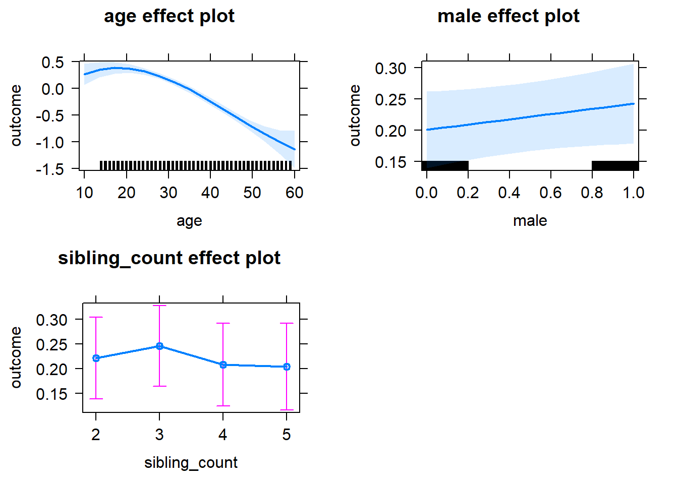
Add Birth Order Linear
Model Summary
tidy(m2_birthorder_linear, conf.int = T, conf.level = 0.995)| effect | group | term | estimate | std.error | statistic | df | p.value | conf.low | conf.high |
|---|---|---|---|---|---|---|---|---|---|
| fixed | NA | (Intercept) | -0.3259 | 0.2608 | -1.25 | 6691 | 0.2115 | -1.058 | 0.4061 |
| fixed | NA | birth_order | 0.001529 | 0.01018 | 0.1502 | 5182 | 0.8806 | -0.02705 | 0.03011 |
| fixed | NA | poly(age, 3, raw = TRUE)1 | 0.0834 | 0.02686 | 3.105 | 6647 | 0.001908 | 0.008012 | 0.1588 |
| fixed | NA | poly(age, 3, raw = TRUE)2 | -0.0029 | 0.0008526 | -3.402 | 6622 | 0.000673 | -0.005294 | -0.0005072 |
| fixed | NA | poly(age, 3, raw = TRUE)3 | 0.00002132 | 0.000008436 | 2.527 | 6574 | 0.01154 | -0.000002365 | 0.000045 |
| fixed | NA | male | 0.0416 | 0.02122 | 1.961 | 6013 | 0.04994 | -0.01795 | 0.1012 |
| fixed | NA | sibling_count3 | 0.02434 | 0.03485 | 0.6984 | 4893 | 0.4849 | -0.07349 | 0.1222 |
| fixed | NA | sibling_count4 | -0.01404 | 0.03714 | -0.3779 | 4905 | 0.7055 | -0.1183 | 0.09022 |
| fixed | NA | sibling_count5 | -0.01924 | 0.04029 | -0.4775 | 5009 | 0.633 | -0.1323 | 0.09385 |
| ran_pars | mother_pidlink | sd__(Intercept) | 0.6048 | NA | NA | NA | NA | NA | NA |
| ran_pars | Residual | sd__Observation | 0.731 | NA | NA | NA | NA | NA | NA |
Coefficient Plot
plot_birthorder2(m2_birthorder_linear, separate = FALSE)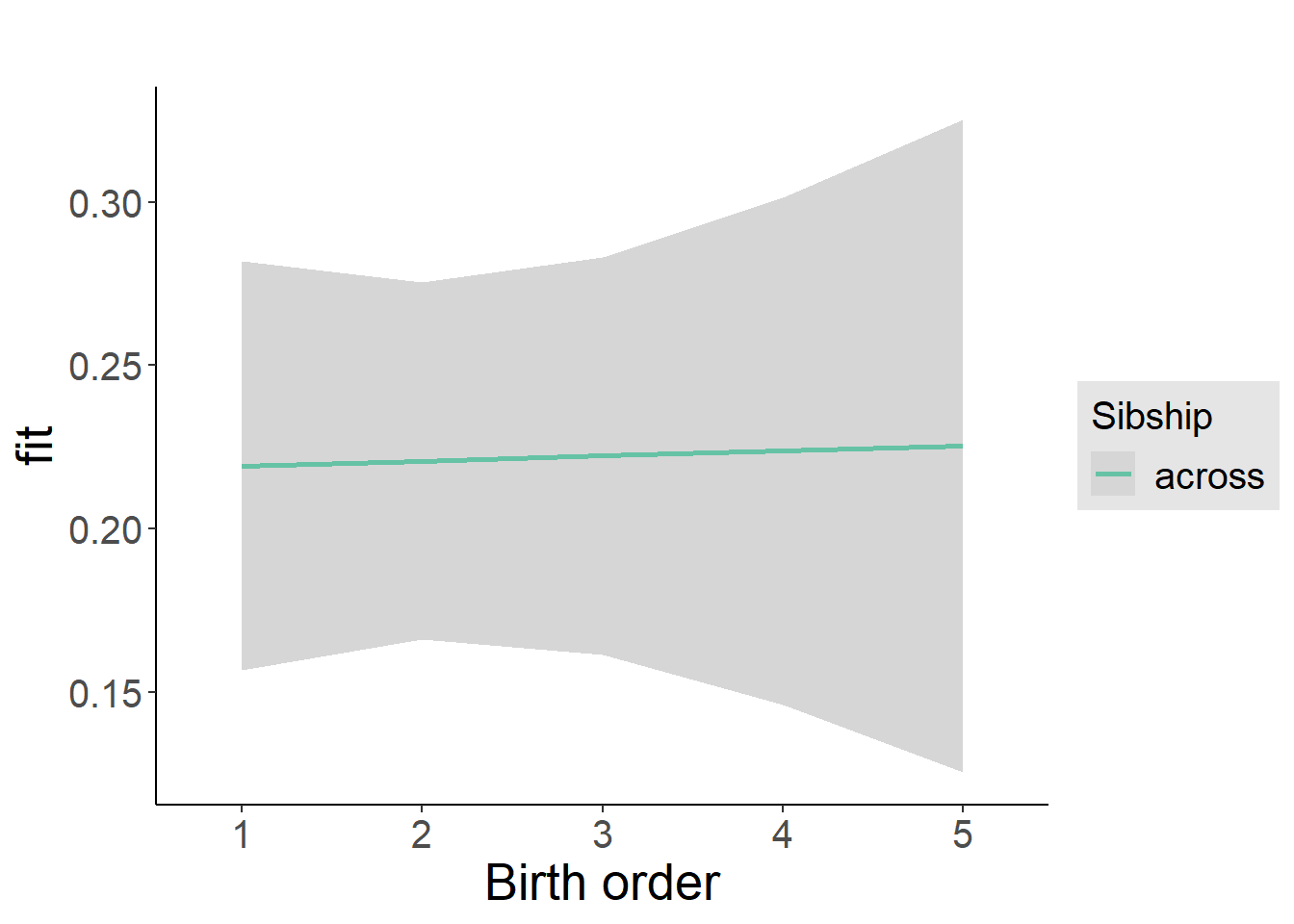
Add Birth Order Factor
Model Summary
m3_birthorder_nonlinear = update(m1_covariates_only, formula = . ~ . + birth_order_nonlinear)
tidy(m3_birthorder_nonlinear, conf.int = T, conf.level = 0.995)| effect | group | term | estimate | std.error | statistic | df | p.value | conf.low | conf.high |
|---|---|---|---|---|---|---|---|---|---|
| fixed | NA | (Intercept) | -0.333 | 0.2625 | -1.268 | 6734 | 0.2048 | -1.07 | 0.404 |
| fixed | NA | poly(age, 3, raw = TRUE)1 | 0.08388 | 0.02704 | 3.102 | 6712 | 0.001929 | 0.007981 | 0.1598 |
| fixed | NA | poly(age, 3, raw = TRUE)2 | -0.002912 | 0.0008597 | -3.387 | 6701 | 0.0007101 | -0.005325 | -0.0004988 |
| fixed | NA | poly(age, 3, raw = TRUE)3 | 0.00002139 | 0.000008516 | 2.512 | 6669 | 0.01202 | -0.00000251 | 0.0000453 |
| fixed | NA | male | 0.04166 | 0.02122 | 1.963 | 6012 | 0.04965 | -0.0179 | 0.1012 |
| fixed | NA | sibling_count3 | 0.02627 | 0.0352 | 0.7465 | 5034 | 0.4554 | -0.07252 | 0.1251 |
| fixed | NA | sibling_count4 | -0.006379 | 0.03752 | -0.17 | 5058 | 0.865 | -0.1117 | 0.09895 |
| fixed | NA | sibling_count5 | -0.02046 | 0.04046 | -0.5057 | 5105 | 0.6131 | -0.1341 | 0.09312 |
| fixed | NA | birth_order_nonlinear2 | 0.009127 | 0.02447 | 0.3729 | 5243 | 0.7092 | -0.05957 | 0.07782 |
| fixed | NA | birth_order_nonlinear3 | -0.004058 | 0.03093 | -0.1312 | 4875 | 0.8956 | -0.09087 | 0.08275 |
| fixed | NA | birth_order_nonlinear4 | -0.02644 | 0.04008 | -0.6596 | 4745 | 0.5095 | -0.1389 | 0.08606 |
| fixed | NA | birth_order_nonlinear5 | 0.06311 | 0.05779 | 1.092 | 4467 | 0.2749 | -0.09912 | 0.2253 |
| ran_pars | mother_pidlink | sd__(Intercept) | 0.604 | NA | NA | NA | NA | NA | NA |
| ran_pars | Residual | sd__Observation | 0.7315 | NA | NA | NA | NA | NA | NA |
Coefficient Plot
plot_birthorder(m3_birthorder_nonlinear, separate = FALSE)
Add Interaction
Model Summary
m4_interaction = update(m3_birthorder_nonlinear, formula = . ~ . - birth_order_nonlinear - sibling_count + count_birth_order)
tidy(m4_interaction, conf.int = T, conf.level = 0.995)| effect | group | term | estimate | std.error | statistic | df | p.value | conf.low | conf.high |
|---|---|---|---|---|---|---|---|---|---|
| fixed | NA | (Intercept) | -0.2996 | 0.2631 | -1.138 | 6739 | 0.255 | -1.038 | 0.4391 |
| fixed | NA | poly(age, 3, raw = TRUE)1 | 0.0817 | 0.02706 | 3.02 | 6713 | 0.002541 | 0.005751 | 0.1577 |
| fixed | NA | poly(age, 3, raw = TRUE)2 | -0.002829 | 0.0008605 | -3.287 | 6706 | 0.001018 | -0.005244 | -0.000413 |
| fixed | NA | poly(age, 3, raw = TRUE)3 | 0.00002046 | 0.000008528 | 2.399 | 6678 | 0.01647 | -0.00000348 | 0.0000444 |
| fixed | NA | male | 0.0421 | 0.02122 | 1.984 | 6001 | 0.04734 | -0.01747 | 0.1017 |
| fixed | NA | count_birth_order2/2 | -0.03765 | 0.04216 | -0.893 | 5516 | 0.3719 | -0.156 | 0.0807 |
| fixed | NA | count_birth_order1/3 | 0.02004 | 0.04291 | 0.467 | 6695 | 0.6405 | -0.1004 | 0.1405 |
| fixed | NA | count_birth_order2/3 | 0.01348 | 0.0474 | 0.2845 | 6859 | 0.776 | -0.1196 | 0.1465 |
| fixed | NA | count_birth_order3/3 | -0.0111 | 0.05256 | -0.2113 | 6890 | 0.8327 | -0.1586 | 0.1364 |
| fixed | NA | count_birth_order1/4 | -0.0239 | 0.0487 | -0.4908 | 6857 | 0.6236 | -0.1606 | 0.1128 |
| fixed | NA | count_birth_order2/4 | 0.01282 | 0.05089 | 0.252 | 6892 | 0.801 | -0.13 | 0.1557 |
| fixed | NA | count_birth_order3/4 | -0.03739 | 0.05447 | -0.6864 | 6874 | 0.4925 | -0.1903 | 0.1155 |
| fixed | NA | count_birth_order4/4 | -0.07971 | 0.05726 | -1.392 | 6838 | 0.164 | -0.2405 | 0.08103 |
| fixed | NA | count_birth_order1/5 | -0.105 | 0.05422 | -1.937 | 6897 | 0.05276 | -0.2572 | 0.04716 |
| fixed | NA | count_birth_order2/5 | -0.006955 | 0.05671 | -0.1226 | 6874 | 0.9024 | -0.1661 | 0.1522 |
| fixed | NA | count_birth_order3/5 | -0.01149 | 0.05812 | -0.1977 | 6834 | 0.8433 | -0.1746 | 0.1517 |
| fixed | NA | count_birth_order4/5 | -0.02821 | 0.0612 | -0.461 | 6754 | 0.6448 | -0.2 | 0.1436 |
| fixed | NA | count_birth_order5/5 | 0.02817 | 0.06237 | 0.4517 | 6733 | 0.6515 | -0.1469 | 0.2033 |
| ran_pars | mother_pidlink | sd__(Intercept) | 0.6045 | NA | NA | NA | NA | NA | NA |
| ran_pars | Residual | sd__Observation | 0.7312 | NA | NA | NA | NA | NA | NA |
Coefficient Plot
plot_birthorder(m4_interaction)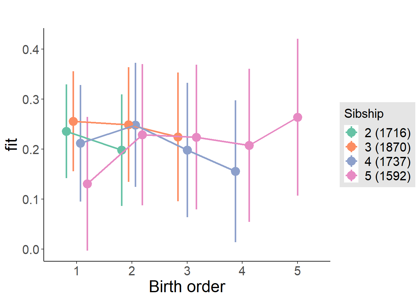
Model Comparison
###### Model 1 - Model 2
anova(m1_covariates_only, m2_birthorder_linear, m3_birthorder_nonlinear, m4_interaction)
## refitting model(s) with ML (instead of REML)| Df | AIC | BIC | logLik | deviance | Chisq | Chi Df | Pr(>Chisq) |
|---|---|---|---|---|---|---|---|
| 10 | 18410 | 18479 | -9195 | 18390 | NA | NA | NA |
| 11 | 18412 | 18487 | -9195 | 18390 | 0.02267 | 1 | 0.8803 |
| 14 | 18416 | 18512 | -9194 | 18388 | 2.301 | 3 | 0.5122 |
| 20 | 18421 | 18558 | -9191 | 18381 | 6.438 | 6 | 0.3759 |
Maternal birth order
outcome_uterus_m1 <- update(m2_birthorder_linear, data = birthorder %>%
                     mutate(sibling_count = sibling_count_uterus_alive_factor,
                            birth_order_nonlinear = birthorder_uterus_alive_factor,
                            birth_order = birthorder_uterus_alive,
                            count_birth_order = count_birthorder_uterus_alive) %>%
                     filter(sibling_count != "1"))
compare_models_markdown(outcome_uterus_m1)
Basic Model
Model Summary
m1_covariates_only <- update(m2_birthorder_linear, formula = . ~ . - birth_order)
tidy(m1_covariates_only, conf.int = T, conf.level = 0.995)| effect | group | term | estimate | std.error | statistic | df | p.value | conf.low | conf.high |
|---|---|---|---|---|---|---|---|---|---|
| fixed | NA | (Intercept) | -0.7436 | 0.4688 | -1.586 | 4282 | 0.1128 | -2.06 | 0.5723 |
| fixed | NA | poly(age, 3, raw = TRUE)1 | 0.1332 | 0.05476 | 2.433 | 4293 | 0.01503 | -0.0205 | 0.2869 |
| fixed | NA | poly(age, 3, raw = TRUE)2 | -0.004198 | 0.00202 | -2.078 | 4310 | 0.03772 | -0.009868 | 0.001472 |
| fixed | NA | poly(age, 3, raw = TRUE)3 | 0.0000361 | 0.00002369 | 1.524 | 4328 | 0.1276 | -0.0000304 | 0.0001026 |
| fixed | NA | male | -0.04436 | 0.02496 | -1.777 | 3982 | 0.07558 | -0.1144 | 0.0257 |
| fixed | NA | sibling_count3 | 0.00115 | 0.03716 | 0.03096 | 3165 | 0.9753 | -0.1032 | 0.1055 |
| fixed | NA | sibling_count4 | -0.07358 | 0.04065 | -1.81 | 2931 | 0.07039 | -0.1877 | 0.04053 |
| fixed | NA | sibling_count5 | -0.1475 | 0.04672 | -3.157 | 2769 | 0.00161 | -0.2786 | -0.01636 |
| ran_pars | mother_pidlink | sd__(Intercept) | 0.5194 | NA | NA | NA | NA | NA | NA |
| ran_pars | Residual | sd__Observation | 0.7004 | NA | NA | NA | NA | NA | NA |
Coefficient Plot
plot(allEffects(m1_covariates_only, confidence.level = 0.995))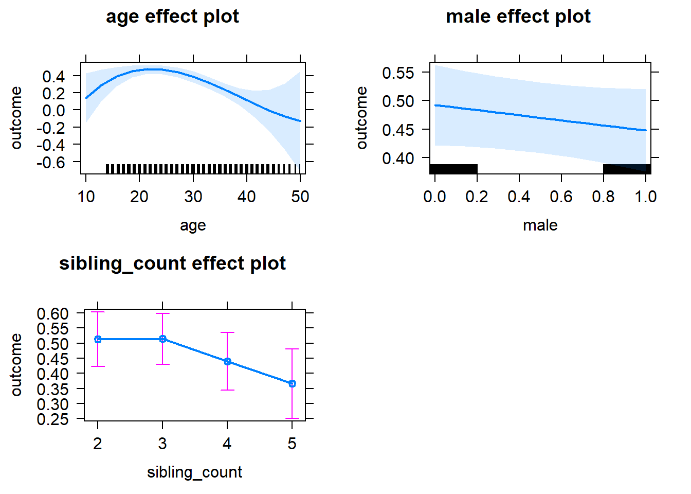
Add Birth Order Linear
Model Summary
tidy(m2_birthorder_linear, conf.int = T, conf.level = 0.995)| effect | group | term | estimate | std.error | statistic | df | p.value | conf.low | conf.high |
|---|---|---|---|---|---|---|---|---|---|
| fixed | NA | (Intercept) | -0.7611 | 0.4694 | -1.621 | 4285 | 0.105 | -2.079 | 0.5565 |
| fixed | NA | birth_order | 0.009772 | 0.01292 | 0.7564 | 3821 | 0.4495 | -0.02649 | 0.04603 |
| fixed | NA | poly(age, 3, raw = TRUE)1 | 0.1337 | 0.05476 | 2.441 | 4293 | 0.01469 | -0.02005 | 0.2874 |
| fixed | NA | poly(age, 3, raw = TRUE)2 | -0.004221 | 0.00202 | -2.089 | 4308 | 0.03674 | -0.009892 | 0.00145 |
| fixed | NA | poly(age, 3, raw = TRUE)3 | 0.00003656 | 0.0000237 | 1.543 | 4326 | 0.123 | -0.00002996 | 0.0001031 |
| fixed | NA | male | -0.04473 | 0.02496 | -1.792 | 3982 | 0.07323 | -0.1148 | 0.02534 |
| fixed | NA | sibling_count3 | -0.003487 | 0.03766 | -0.0926 | 3220 | 0.9262 | -0.1092 | 0.1022 |
| fixed | NA | sibling_count4 | -0.08445 | 0.04311 | -1.959 | 3117 | 0.05024 | -0.2055 | 0.03658 |
| fixed | NA | sibling_count5 | -0.1654 | 0.05239 | -3.158 | 3206 | 0.001605 | -0.3125 | -0.01837 |
| ran_pars | mother_pidlink | sd__(Intercept) | 0.5191 | NA | NA | NA | NA | NA | NA |
| ran_pars | Residual | sd__Observation | 0.7006 | NA | NA | NA | NA | NA | NA |
Coefficient Plot
plot_birthorder2(m2_birthorder_linear, separate = FALSE)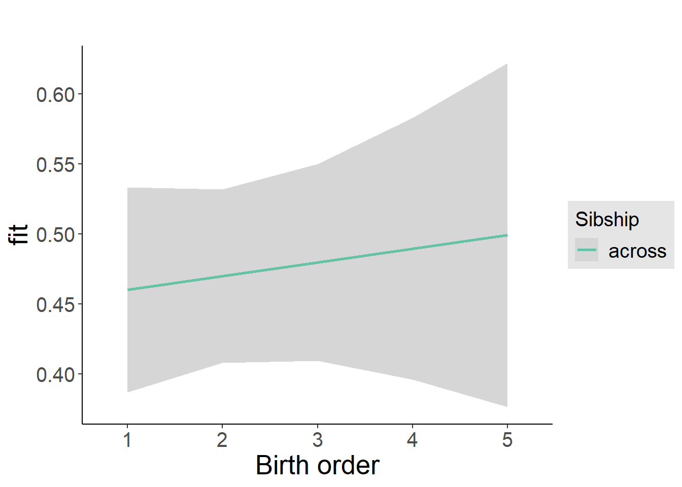
Add Birth Order Factor
Model Summary
m3_birthorder_nonlinear = update(m1_covariates_only, formula = . ~ . + birth_order_nonlinear)
tidy(m3_birthorder_nonlinear, conf.int = T, conf.level = 0.995)| effect | group | term | estimate | std.error | statistic | df | p.value | conf.low | conf.high |
|---|---|---|---|---|---|---|---|---|---|
| fixed | NA | (Intercept) | -0.8081 | 0.4706 | -1.717 | 4305 | 0.08599 | -2.129 | 0.5127 |
| fixed | NA | poly(age, 3, raw = TRUE)1 | 0.1386 | 0.05489 | 2.525 | 4309 | 0.01161 | -0.01548 | 0.2927 |
| fixed | NA | poly(age, 3, raw = TRUE)2 | -0.004396 | 0.002024 | -2.171 | 4321 | 0.02996 | -0.01008 | 0.001287 |
| fixed | NA | poly(age, 3, raw = TRUE)3 | 0.00003844 | 0.00002374 | 1.619 | 4335 | 0.1054 | -0.00002819 | 0.0001051 |
| fixed | NA | male | -0.04387 | 0.02497 | -1.757 | 3975 | 0.07899 | -0.1139 | 0.02622 |
| fixed | NA | sibling_count3 | -0.003513 | 0.0381 | -0.0922 | 3317 | 0.9265 | -0.1105 | 0.1034 |
| fixed | NA | sibling_count4 | -0.07787 | 0.04362 | -1.785 | 3204 | 0.07437 | -0.2003 | 0.04459 |
| fixed | NA | sibling_count5 | -0.1555 | 0.05312 | -2.928 | 3301 | 0.003439 | -0.3046 | -0.006406 |
| fixed | NA | birth_order_nonlinear2 | 0.05449 | 0.02872 | 1.898 | 3157 | 0.05783 | -0.02611 | 0.1351 |
| fixed | NA | birth_order_nonlinear3 | 0.02076 | 0.0368 | 0.564 | 3324 | 0.5728 | -0.08254 | 0.124 |
| fixed | NA | birth_order_nonlinear4 | 0.01169 | 0.04992 | 0.2342 | 3501 | 0.8149 | -0.1284 | 0.1518 |
| fixed | NA | birth_order_nonlinear5 | 0.04547 | 0.07653 | 0.5942 | 3272 | 0.5524 | -0.1693 | 0.2603 |
| ran_pars | mother_pidlink | sd__(Intercept) | 0.5195 | NA | NA | NA | NA | NA | NA |
| ran_pars | Residual | sd__Observation | 0.7004 | NA | NA | NA | NA | NA | NA |
Coefficient Plot
plot_birthorder(m3_birthorder_nonlinear, separate = FALSE)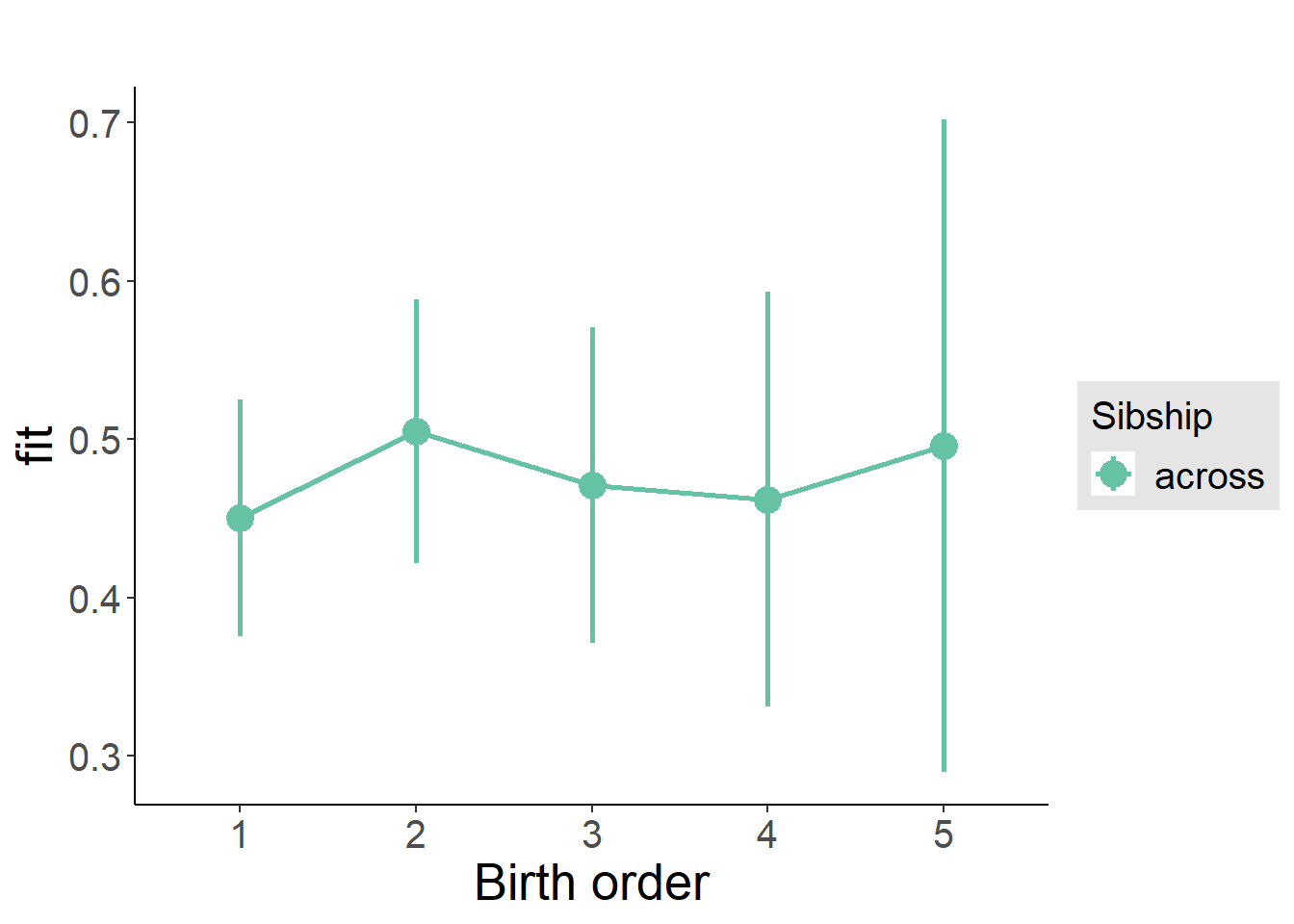
Add Interaction
Model Summary
m4_interaction = update(m3_birthorder_nonlinear, formula = . ~ . - birth_order_nonlinear - sibling_count + count_birth_order)
tidy(m4_interaction, conf.int = T, conf.level = 0.995)| effect | group | term | estimate | std.error | statistic | df | p.value | conf.low | conf.high |
|---|---|---|---|---|---|---|---|---|---|
| fixed | NA | (Intercept) | -0.8021 | 0.471 | -1.703 | 4302 | 0.08866 | -2.124 | 0.5201 |
| fixed | NA | poly(age, 3, raw = TRUE)1 | 0.1375 | 0.05493 | 2.503 | 4303 | 0.01236 | -0.01671 | 0.2917 |
| fixed | NA | poly(age, 3, raw = TRUE)2 | -0.004338 | 0.002026 | -2.141 | 4315 | 0.03234 | -0.01003 | 0.00135 |
| fixed | NA | poly(age, 3, raw = TRUE)3 | 0.00003759 | 0.00002376 | 1.582 | 4329 | 0.1138 | -0.00002912 | 0.0001043 |
| fixed | NA | male | -0.04431 | 0.025 | -1.773 | 3970 | 0.07637 | -0.1145 | 0.02586 |
| fixed | NA | count_birth_order2/2 | 0.05411 | 0.04991 | 1.084 | 3498 | 0.2784 | -0.08599 | 0.1942 |
| fixed | NA | count_birth_order1/3 | -0.004653 | 0.04659 | -0.09986 | 4345 | 0.9205 | -0.1354 | 0.1261 |
| fixed | NA | count_birth_order2/3 | 0.04349 | 0.05027 | 0.8651 | 4411 | 0.387 | -0.09761 | 0.1846 |
| fixed | NA | count_birth_order3/3 | 0.0296 | 0.05593 | 0.5291 | 4401 | 0.5967 | -0.1274 | 0.1866 |
| fixed | NA | count_birth_order1/4 | -0.09954 | 0.0569 | -1.749 | 4406 | 0.08032 | -0.2593 | 0.06019 |
| fixed | NA | count_birth_order2/4 | -0.01884 | 0.05842 | -0.3224 | 4405 | 0.7471 | -0.1828 | 0.1451 |
| fixed | NA | count_birth_order3/4 | -0.06075 | 0.06096 | -0.9965 | 4362 | 0.3191 | -0.2319 | 0.1104 |
| fixed | NA | count_birth_order4/4 | -0.03633 | 0.06357 | -0.5715 | 4349 | 0.5677 | -0.2148 | 0.1421 |
| fixed | NA | count_birth_order1/5 | -0.1058 | 0.07594 | -1.393 | 4382 | 0.1638 | -0.3189 | 0.1074 |
| fixed | NA | count_birth_order2/5 | -0.08542 | 0.08138 | -1.05 | 4240 | 0.2939 | -0.3138 | 0.143 |
| fixed | NA | count_birth_order3/5 | -0.1551 | 0.07613 | -2.037 | 4265 | 0.04168 | -0.3688 | 0.0586 |
| fixed | NA | count_birth_order4/5 | -0.1873 | 0.07361 | -2.545 | 4321 | 0.01097 | -0.3939 | 0.01931 |
| fixed | NA | count_birth_order5/5 | -0.1121 | 0.07545 | -1.485 | 4290 | 0.1375 | -0.3239 | 0.09971 |
| ran_pars | mother_pidlink | sd__(Intercept) | 0.5185 | NA | NA | NA | NA | NA | NA |
| ran_pars | Residual | sd__Observation | 0.7014 | NA | NA | NA | NA | NA | NA |
Coefficient Plot
plot_birthorder(m4_interaction)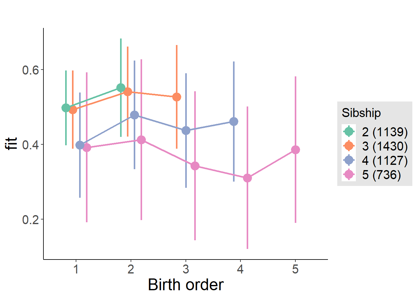
Model Comparison
###### Model 1 - Model 2
anova(m1_covariates_only, m2_birthorder_linear, m3_birthorder_nonlinear, m4_interaction)
## refitting model(s) with ML (instead of REML)| Df | AIC | BIC | logLik | deviance | Chisq | Chi Df | Pr(>Chisq) |
|---|---|---|---|---|---|---|---|
| 10 | 11166 | 11230 | -5573 | 11146 | NA | NA | NA |
| 11 | 11167 | 11238 | -5573 | 11145 | 0.5738 | 1 | 0.4488 |
| 14 | 11170 | 11260 | -5571 | 11142 | 3.264 | 3 | 0.3527 |
| 20 | 11180 | 11308 | -5570 | 11140 | 1.949 | 6 | 0.9243 |
Maternal pregnancy order
outcome_preg_m1 <- update(m2_birthorder_linear, data = birthorder %>%
  mutate(sibling_count = sibling_count_uterus_preg_factor,
         birth_order_nonlinear = birthorder_uterus_preg_factor,
         birth_order = birthorder_uterus_preg,
         count_birth_order = count_birthorder_uterus_preg
         ) %>%
    filter(sibling_count != "1"))
compare_models_markdown(outcome_preg_m1)
Basic Model
Model Summary
m1_covariates_only <- update(m2_birthorder_linear, formula = . ~ . - birth_order)
tidy(m1_covariates_only, conf.int = T, conf.level = 0.995)| effect | group | term | estimate | std.error | statistic | df | p.value | conf.low | conf.high |
|---|---|---|---|---|---|---|---|---|---|
| fixed | NA | (Intercept) | -0.7435 | 0.4819 | -1.543 | 3975 | 0.123 | -2.096 | 0.6092 |
| fixed | NA | poly(age, 3, raw = TRUE)1 | 0.1331 | 0.05632 | 2.363 | 3985 | 0.0182 | -0.02504 | 0.2912 |
| fixed | NA | poly(age, 3, raw = TRUE)2 | -0.004244 | 0.002078 | -2.042 | 4000 | 0.0412 | -0.01008 | 0.00159 |
| fixed | NA | poly(age, 3, raw = TRUE)3 | 0.00003669 | 0.00002437 | 1.505 | 4018 | 0.1323 | -0.00003173 | 0.0001051 |
| fixed | NA | male | -0.03882 | 0.02587 | -1.501 | 3697 | 0.1334 | -0.1114 | 0.03378 |
| fixed | NA | sibling_count3 | 0.007909 | 0.03991 | 0.1982 | 3012 | 0.8429 | -0.1041 | 0.1199 |
| fixed | NA | sibling_count4 | -0.03952 | 0.04268 | -0.9261 | 2835 | 0.3544 | -0.1593 | 0.08027 |
| fixed | NA | sibling_count5 | -0.07459 | 0.04593 | -1.624 | 2669 | 0.1045 | -0.2035 | 0.05433 |
| ran_pars | mother_pidlink | sd__(Intercept) | 0.515 | NA | NA | NA | NA | NA | NA |
| ran_pars | Residual | sd__Observation | 0.7004 | NA | NA | NA | NA | NA | NA |
Coefficient Plot
plot(allEffects(m1_covariates_only, confidence.level = 0.995))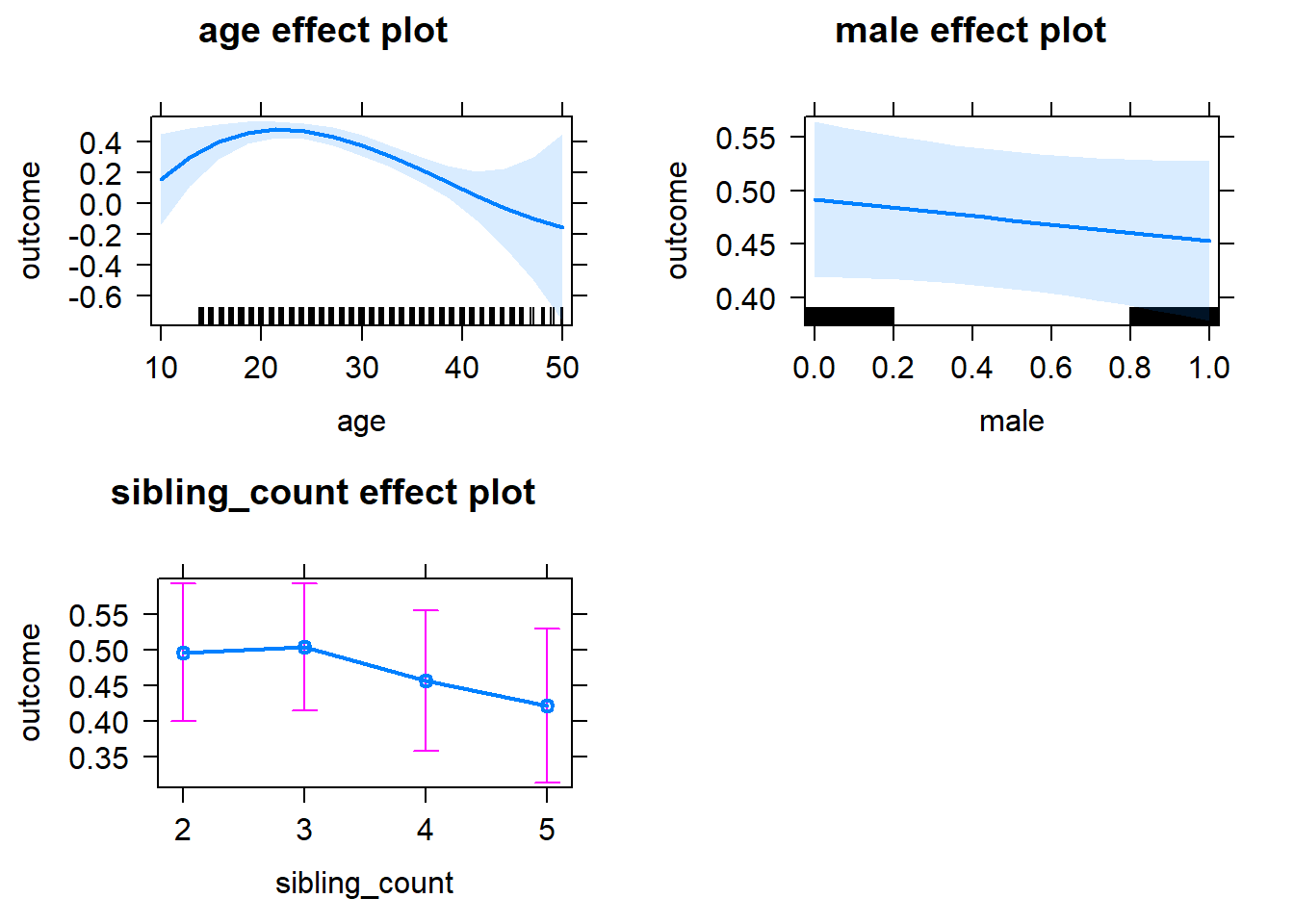
Add Birth Order Linear
Model Summary
tidy(m2_birthorder_linear, conf.int = T, conf.level = 0.995)| effect | group | term | estimate | std.error | statistic | df | p.value | conf.low | conf.high |
|---|---|---|---|---|---|---|---|---|---|
| fixed | NA | (Intercept) | -0.7403 | 0.4825 | -1.534 | 3976 | 0.125 | -2.095 | 0.6139 |
| fixed | NA | birth_order | -0.001929 | 0.01298 | -0.1485 | 3632 | 0.8819 | -0.03837 | 0.03452 |
| fixed | NA | poly(age, 3, raw = TRUE)1 | 0.133 | 0.05633 | 2.361 | 3983 | 0.01826 | -0.02511 | 0.2911 |
| fixed | NA | poly(age, 3, raw = TRUE)2 | -0.004241 | 0.002079 | -2.04 | 3998 | 0.04137 | -0.01008 | 0.001593 |
| fixed | NA | poly(age, 3, raw = TRUE)3 | 0.00003661 | 0.00002438 | 1.502 | 4015 | 0.1332 | -0.00003182 | 0.000105 |
| fixed | NA | male | -0.03877 | 0.02587 | -1.499 | 3696 | 0.134 | -0.1114 | 0.03385 |
| fixed | NA | sibling_count3 | 0.00883 | 0.04039 | 0.2186 | 3052 | 0.827 | -0.1046 | 0.1222 |
| fixed | NA | sibling_count4 | -0.03746 | 0.04489 | -0.8346 | 2976 | 0.404 | -0.1635 | 0.08854 |
| fixed | NA | sibling_count5 | -0.07133 | 0.0509 | -1.401 | 3002 | 0.1612 | -0.2142 | 0.07155 |
| ran_pars | mother_pidlink | sd__(Intercept) | 0.515 | NA | NA | NA | NA | NA | NA |
| ran_pars | Residual | sd__Observation | 0.7005 | NA | NA | NA | NA | NA | NA |
Coefficient Plot
plot_birthorder2(m2_birthorder_linear, separate = FALSE)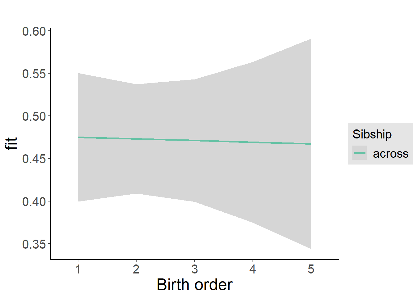
Add Birth Order Factor
Model Summary
m3_birthorder_nonlinear = update(m1_covariates_only, formula = . ~ . + birth_order_nonlinear)
tidy(m3_birthorder_nonlinear, conf.int = T, conf.level = 0.995)| effect | group | term | estimate | std.error | statistic | df | p.value | conf.low | conf.high |
|---|---|---|---|---|---|---|---|---|---|
| fixed | NA | (Intercept) | -0.8051 | 0.4835 | -1.665 | 3998 | 0.09595 | -2.162 | 0.552 |
| fixed | NA | poly(age, 3, raw = TRUE)1 | 0.1381 | 0.05643 | 2.446 | 4000 | 0.01447 | -0.02035 | 0.2965 |
| fixed | NA | poly(age, 3, raw = TRUE)2 | -0.004421 | 0.002082 | -2.123 | 4012 | 0.03378 | -0.01027 | 0.001423 |
| fixed | NA | poly(age, 3, raw = TRUE)3 | 0.00003854 | 0.00002441 | 1.579 | 4025 | 0.1145 | -0.00002999 | 0.0001071 |
| fixed | NA | male | -0.03757 | 0.02586 | -1.453 | 3689 | 0.1464 | -0.1102 | 0.03503 |
| fixed | NA | sibling_count3 | 0.009672 | 0.04084 | 0.2368 | 3135 | 0.8128 | -0.105 | 0.1243 |
| fixed | NA | sibling_count4 | -0.02811 | 0.04538 | -0.6194 | 3053 | 0.5357 | -0.1555 | 0.09927 |
| fixed | NA | sibling_count5 | -0.06211 | 0.05131 | -1.211 | 3056 | 0.2262 | -0.2062 | 0.08192 |
| fixed | NA | birth_order_nonlinear2 | 0.05758 | 0.02997 | 1.921 | 2997 | 0.05477 | -0.02654 | 0.1417 |
| fixed | NA | birth_order_nonlinear3 | -0.007206 | 0.03803 | -0.1895 | 3146 | 0.8497 | -0.114 | 0.09955 |
| fixed | NA | birth_order_nonlinear4 | -0.03213 | 0.05075 | -0.633 | 3290 | 0.5268 | -0.1746 | 0.1103 |
| fixed | NA | birth_order_nonlinear5 | 0.02177 | 0.07352 | 0.296 | 3090 | 0.7672 | -0.1846 | 0.2281 |
| ran_pars | mother_pidlink | sd__(Intercept) | 0.5157 | NA | NA | NA | NA | NA | NA |
| ran_pars | Residual | sd__Observation | 0.6998 | NA | NA | NA | NA | NA | NA |
Coefficient Plot
plot_birthorder(m3_birthorder_nonlinear, separate = FALSE)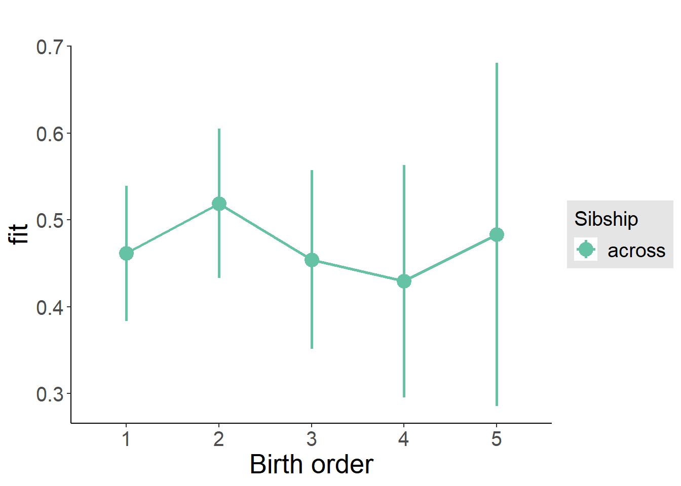
Add Interaction
Model Summary
m4_interaction = update(m3_birthorder_nonlinear, formula = . ~ . - birth_order_nonlinear - sibling_count + count_birth_order)
tidy(m4_interaction, conf.int = T, conf.level = 0.995)| effect | group | term | estimate | std.error | statistic | df | p.value | conf.low | conf.high |
|---|---|---|---|---|---|---|---|---|---|
| fixed | NA | (Intercept) | -0.8036 | 0.4838 | -1.661 | 3994 | 0.09682 | -2.162 | 0.5546 |
| fixed | NA | poly(age, 3, raw = TRUE)1 | 0.1364 | 0.05645 | 2.416 | 3994 | 0.01575 | -0.02209 | 0.2948 |
| fixed | NA | poly(age, 3, raw = TRUE)2 | -0.004347 | 0.002083 | -2.087 | 4006 | 0.03695 | -0.01019 | 0.0015 |
| fixed | NA | poly(age, 3, raw = TRUE)3 | 0.00003753 | 0.00002443 | 1.536 | 4019 | 0.1245 | -0.00003104 | 0.0001061 |
| fixed | NA | male | -0.0392 | 0.02588 | -1.515 | 3682 | 0.1298 | -0.1118 | 0.03343 |
| fixed | NA | count_birth_order2/2 | 0.09254 | 0.05464 | 1.694 | 3313 | 0.09045 | -0.06085 | 0.2459 |
| fixed | NA | count_birth_order1/3 | 0.04149 | 0.05028 | 0.8251 | 4041 | 0.4094 | -0.09965 | 0.1826 |
| fixed | NA | count_birth_order2/3 | 0.03037 | 0.05388 | 0.5636 | 4094 | 0.573 | -0.1209 | 0.1816 |
| fixed | NA | count_birth_order3/3 | 0.04362 | 0.0603 | 0.7233 | 4085 | 0.4695 | -0.1257 | 0.2129 |
| fixed | NA | count_birth_order1/4 | -0.06879 | 0.05946 | -1.157 | 4089 | 0.2474 | -0.2357 | 0.09812 |
| fixed | NA | count_birth_order2/4 | 0.09198 | 0.06038 | 1.524 | 4095 | 0.1277 | -0.07749 | 0.2615 |
| fixed | NA | count_birth_order3/4 | -0.0285 | 0.06509 | -0.4379 | 4036 | 0.6615 | -0.2112 | 0.1542 |
| fixed | NA | count_birth_order4/4 | -0.03212 | 0.06728 | -0.4775 | 4038 | 0.633 | -0.221 | 0.1567 |
| fixed | NA | count_birth_order1/5 | 0.01199 | 0.06973 | 0.172 | 4095 | 0.8635 | -0.1837 | 0.2077 |
| fixed | NA | count_birth_order2/5 | -0.008682 | 0.07461 | -0.1164 | 3996 | 0.9074 | -0.2181 | 0.2008 |
| fixed | NA | count_birth_order3/5 | -0.09928 | 0.07207 | -1.378 | 3999 | 0.1684 | -0.3016 | 0.103 |
| fixed | NA | count_birth_order4/5 | -0.1043 | 0.07462 | -1.397 | 3954 | 0.1625 | -0.3137 | 0.1052 |
| fixed | NA | count_birth_order5/5 | -0.03106 | 0.07443 | -0.4173 | 3966 | 0.6765 | -0.24 | 0.1779 |
| ran_pars | mother_pidlink | sd__(Intercept) | 0.5155 | NA | NA | NA | NA | NA | NA |
| ran_pars | Residual | sd__Observation | 0.6997 | NA | NA | NA | NA | NA | NA |
Coefficient Plot
plot_birthorder(m4_interaction)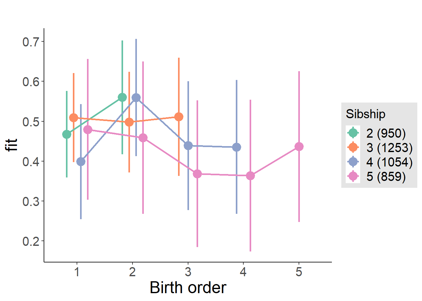
Model Comparison
###### Model 1 - Model 2
anova(m1_covariates_only, m2_birthorder_linear, m3_birthorder_nonlinear, m4_interaction)
## refitting model(s) with ML (instead of REML)| Df | AIC | BIC | logLik | deviance | Chisq | Chi Df | Pr(>Chisq) |
|---|---|---|---|---|---|---|---|
| 10 | 10355 | 10418 | -5167 | 10335 | NA | NA | NA |
| 11 | 10357 | 10426 | -5167 | 10335 | 0.02194 | 1 | 0.8823 |
| 14 | 10357 | 10446 | -5165 | 10329 | 5.805 | 3 | 0.1215 |
| 20 | 10362 | 10488 | -5161 | 10322 | 7.515 | 6 | 0.2758 |
Parental full sibling order
outcome_parental_m1 <- update(m2_birthorder_linear, data = birthorder %>%
  mutate(sibling_count = sibling_count_genes_factor,
         birth_order_nonlinear = birthorder_genes_factor,
         birth_order = birthorder_genes,
         count_birth_order = count_birthorder_genes
         ) %>%
      filter(sibling_count != "1"))
compare_models_markdown(outcome_parental_m1)
Basic Model
Model Summary
m1_covariates_only <- update(m2_birthorder_linear, formula = . ~ . - birth_order)
tidy(m1_covariates_only, conf.int = T, conf.level = 0.995)| effect | group | term | estimate | std.error | statistic | df | p.value | conf.low | conf.high |
|---|---|---|---|---|---|---|---|---|---|
| fixed | NA | (Intercept) | -0.8161 | 0.471 | -1.733 | 4271 | 0.0832 | -2.138 | 0.5059 |
| fixed | NA | poly(age, 3, raw = TRUE)1 | 0.1401 | 0.05508 | 2.543 | 4282 | 0.01103 | -0.01455 | 0.2947 |
| fixed | NA | poly(age, 3, raw = TRUE)2 | -0.00443 | 0.002035 | -2.177 | 4297 | 0.02952 | -0.01014 | 0.001281 |
| fixed | NA | poly(age, 3, raw = TRUE)3 | 0.00003822 | 0.00002391 | 1.599 | 4314 | 0.1099 | -0.00002888 | 0.0001053 |
| fixed | NA | male | -0.04486 | 0.0249 | -1.802 | 3983 | 0.07169 | -0.1148 | 0.02504 |
| fixed | NA | sibling_count3 | 0.01733 | 0.03647 | 0.4751 | 3184 | 0.6347 | -0.08506 | 0.1197 |
| fixed | NA | sibling_count4 | -0.05818 | 0.0401 | -1.451 | 2969 | 0.1469 | -0.1707 | 0.05438 |
| fixed | NA | sibling_count5 | -0.12 | 0.04769 | -2.517 | 2735 | 0.01191 | -0.2539 | 0.01386 |
| ran_pars | mother_pidlink | sd__(Intercept) | 0.5138 | NA | NA | NA | NA | NA | NA |
| ran_pars | Residual | sd__Observation | 0.6993 | NA | NA | NA | NA | NA | NA |
Coefficient Plot
plot(allEffects(m1_covariates_only, confidence.level = 0.995))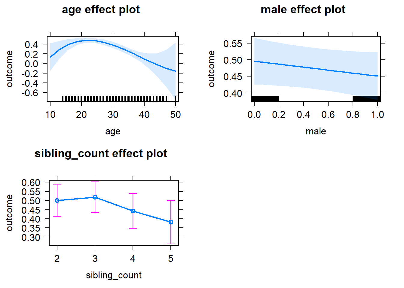
Add Birth Order Linear
Model Summary
tidy(m2_birthorder_linear, conf.int = T, conf.level = 0.995)| effect | group | term | estimate | std.error | statistic | df | p.value | conf.low | conf.high |
|---|---|---|---|---|---|---|---|---|---|
| fixed | NA | (Intercept) | -0.8377 | 0.4716 | -1.776 | 4274 | 0.07574 | -2.161 | 0.486 |
| fixed | NA | birth_order | 0.01203 | 0.01302 | 0.9236 | 3791 | 0.3557 | -0.02453 | 0.04858 |
| fixed | NA | poly(age, 3, raw = TRUE)1 | 0.1406 | 0.05509 | 2.553 | 4281 | 0.01071 | -0.01399 | 0.2953 |
| fixed | NA | poly(age, 3, raw = TRUE)2 | -0.004458 | 0.002035 | -2.191 | 4296 | 0.02852 | -0.01017 | 0.001254 |
| fixed | NA | poly(age, 3, raw = TRUE)3 | 0.0000388 | 0.00002391 | 1.622 | 4312 | 0.1048 | -0.00002833 | 0.0001059 |
| fixed | NA | male | -0.0452 | 0.0249 | -1.815 | 3982 | 0.06959 | -0.1151 | 0.0247 |
| fixed | NA | sibling_count3 | 0.01158 | 0.037 | 0.3131 | 3235 | 0.7542 | -0.09227 | 0.1154 |
| fixed | NA | sibling_count4 | -0.07149 | 0.04261 | -1.678 | 3167 | 0.09347 | -0.1911 | 0.04811 |
| fixed | NA | sibling_count5 | -0.1411 | 0.05289 | -2.669 | 3122 | 0.007658 | -0.2896 | 0.007326 |
| ran_pars | mother_pidlink | sd__(Intercept) | 0.5135 | NA | NA | NA | NA | NA | NA |
| ran_pars | Residual | sd__Observation | 0.6995 | NA | NA | NA | NA | NA | NA |
Coefficient Plot
plot_birthorder2(m2_birthorder_linear, separate = FALSE)
Add Birth Order Factor
Model Summary
m3_birthorder_nonlinear = update(m1_covariates_only, formula = . ~ . + birth_order_nonlinear)
tidy(m3_birthorder_nonlinear, conf.int = T, conf.level = 0.995)| effect | group | term | estimate | std.error | statistic | df | p.value | conf.low | conf.high |
|---|---|---|---|---|---|---|---|---|---|
| fixed | NA | (Intercept) | -0.8837 | 0.4727 | -1.87 | 4294 | 0.0616 | -2.211 | 0.4431 |
| fixed | NA | poly(age, 3, raw = TRUE)1 | 0.1457 | 0.05521 | 2.638 | 4297 | 0.008361 | -0.009313 | 0.3006 |
| fixed | NA | poly(age, 3, raw = TRUE)2 | -0.004635 | 0.002039 | -2.273 | 4308 | 0.02305 | -0.01036 | 0.001088 |
| fixed | NA | poly(age, 3, raw = TRUE)3 | 0.00004069 | 0.00002395 | 1.699 | 4320 | 0.0894 | -0.00002654 | 0.0001079 |
| fixed | NA | male | -0.04487 | 0.0249 | -1.802 | 3974 | 0.07164 | -0.1148 | 0.02503 |
| fixed | NA | sibling_count3 | 0.01272 | 0.03746 | 0.3396 | 3336 | 0.7342 | -0.09242 | 0.1179 |
| fixed | NA | sibling_count4 | -0.06832 | 0.04313 | -1.584 | 3256 | 0.1133 | -0.1894 | 0.05274 |
| fixed | NA | sibling_count5 | -0.127 | 0.05379 | -2.36 | 3231 | 0.01831 | -0.278 | 0.02403 |
| fixed | NA | birth_order_nonlinear2 | 0.0573 | 0.02844 | 2.015 | 3154 | 0.04403 | -0.02254 | 0.1371 |
| fixed | NA | birth_order_nonlinear3 | 0.02371 | 0.03653 | 0.6491 | 3309 | 0.5163 | -0.07883 | 0.1263 |
| fixed | NA | birth_order_nonlinear4 | 0.03831 | 0.05064 | 0.7565 | 3465 | 0.4494 | -0.1038 | 0.1805 |
| fixed | NA | birth_order_nonlinear5 | 0.01316 | 0.0818 | 0.1609 | 3321 | 0.8722 | -0.2164 | 0.2428 |
| ran_pars | mother_pidlink | sd__(Intercept) | 0.5141 | NA | NA | NA | NA | NA | NA |
| ran_pars | Residual | sd__Observation | 0.6991 | NA | NA | NA | NA | NA | NA |
Coefficient Plot
plot_birthorder(m3_birthorder_nonlinear, separate = FALSE)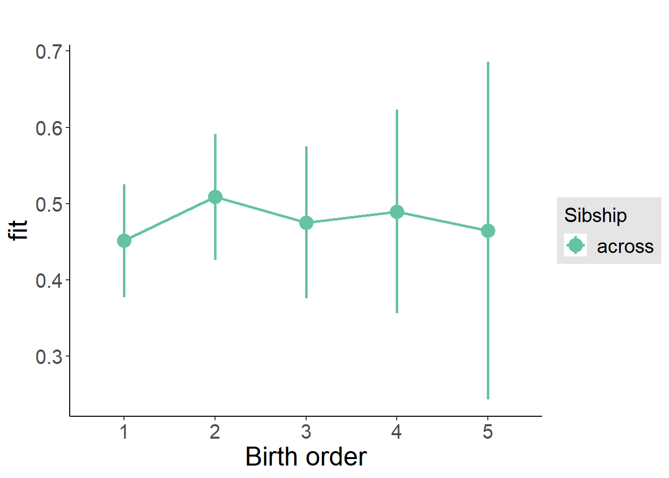
Add Interaction
Model Summary
m4_interaction = update(m3_birthorder_nonlinear, formula = . ~ . - birth_order_nonlinear - sibling_count + count_birth_order)
tidy(m4_interaction, conf.int = T, conf.level = 0.995)| effect | group | term | estimate | std.error | statistic | df | p.value | conf.low | conf.high |
|---|---|---|---|---|---|---|---|---|---|
| fixed | NA | (Intercept) | -0.8808 | 0.4732 | -1.861 | 4291 | 0.06274 | -2.209 | 0.4474 |
| fixed | NA | poly(age, 3, raw = TRUE)1 | 0.1448 | 0.05525 | 2.621 | 4291 | 0.008791 | -0.01026 | 0.2999 |
| fixed | NA | poly(age, 3, raw = TRUE)2 | -0.00459 | 0.002041 | -2.249 | 4301 | 0.02455 | -0.01032 | 0.001138 |
| fixed | NA | poly(age, 3, raw = TRUE)3 | 0.00004 | 0.00002398 | 1.668 | 4314 | 0.09534 | -0.0000273 | 0.0001073 |
| fixed | NA | male | -0.04527 | 0.02493 | -1.816 | 3968 | 0.06945 | -0.1152 | 0.02471 |
| fixed | NA | count_birth_order2/2 | 0.06104 | 0.04831 | 1.264 | 3438 | 0.2065 | -0.07456 | 0.1966 |
| fixed | NA | count_birth_order1/3 | 0.01191 | 0.0458 | 0.26 | 4336 | 0.7949 | -0.1167 | 0.1405 |
| fixed | NA | count_birth_order2/3 | 0.06666 | 0.04995 | 1.334 | 4402 | 0.1821 | -0.07356 | 0.2069 |
| fixed | NA | count_birth_order3/3 | 0.04796 | 0.05471 | 0.8766 | 4385 | 0.3807 | -0.1056 | 0.2015 |
| fixed | NA | count_birth_order1/4 | -0.08141 | 0.05677 | -1.434 | 4400 | 0.1516 | -0.2408 | 0.07794 |
| fixed | NA | count_birth_order2/4 | -0.01152 | 0.05804 | -0.1985 | 4385 | 0.8427 | -0.1745 | 0.1514 |
| fixed | NA | count_birth_order3/4 | -0.04143 | 0.06011 | -0.6893 | 4345 | 0.4907 | -0.2102 | 0.1273 |
| fixed | NA | count_birth_order4/4 | -0.007317 | 0.06337 | -0.1155 | 4311 | 0.9081 | -0.1852 | 0.1706 |
| fixed | NA | count_birth_order1/5 | -0.08094 | 0.07556 | -1.071 | 4385 | 0.2841 | -0.293 | 0.1312 |
| fixed | NA | count_birth_order2/5 | -0.05516 | 0.08349 | -0.6606 | 4206 | 0.5089 | -0.2895 | 0.1792 |
| fixed | NA | count_birth_order3/5 | -0.1308 | 0.07923 | -1.651 | 4234 | 0.09876 | -0.3532 | 0.09157 |
| fixed | NA | count_birth_order4/5 | -0.1222 | 0.07667 | -1.594 | 4293 | 0.111 | -0.3374 | 0.09301 |
| fixed | NA | count_birth_order5/5 | -0.1139 | 0.0803 | -1.419 | 4253 | 0.156 | -0.3394 | 0.1115 |
| ran_pars | mother_pidlink | sd__(Intercept) | 0.5133 | NA | NA | NA | NA | NA | NA |
| ran_pars | Residual | sd__Observation | 0.7001 | NA | NA | NA | NA | NA | NA |
Coefficient Plot
plot_birthorder(m4_interaction)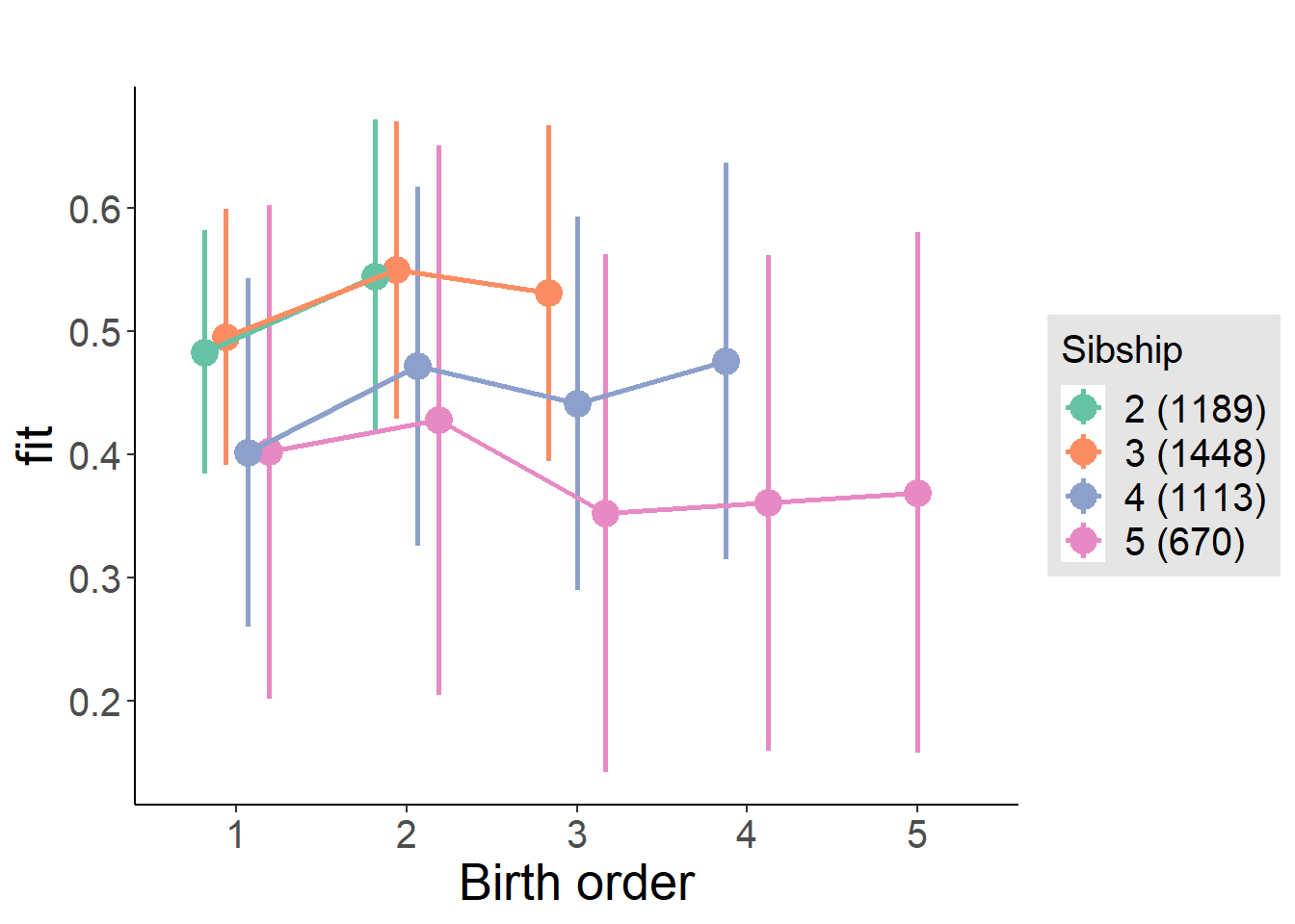
Model Comparison
###### Model 1 - Model 2
anova(m1_covariates_only, m2_birthorder_linear, m3_birthorder_nonlinear, m4_interaction)
## refitting model(s) with ML (instead of REML)| Df | AIC | BIC | logLik | deviance | Chisq | Chi Df | Pr(>Chisq) |
|---|---|---|---|---|---|---|---|
| 10 | 11095 | 11159 | -5538 | 11075 | NA | NA | NA |
| 11 | 11096 | 11167 | -5537 | 11074 | 0.8553 | 1 | 0.3551 |
| 14 | 11099 | 11189 | -5535 | 11071 | 3.32 | 3 | 0.3449 |
| 20 | 11110 | 11238 | -5535 | 11070 | 1.346 | 6 | 0.969 |
Compare birth order specifications
library(coefplot)
multiplot(outcome_naive_m1, outcome_preg_m1, outcome_uterus_m1, outcome_parental_m1, dodgeHeight = 0.6,
          intercept = FALSE)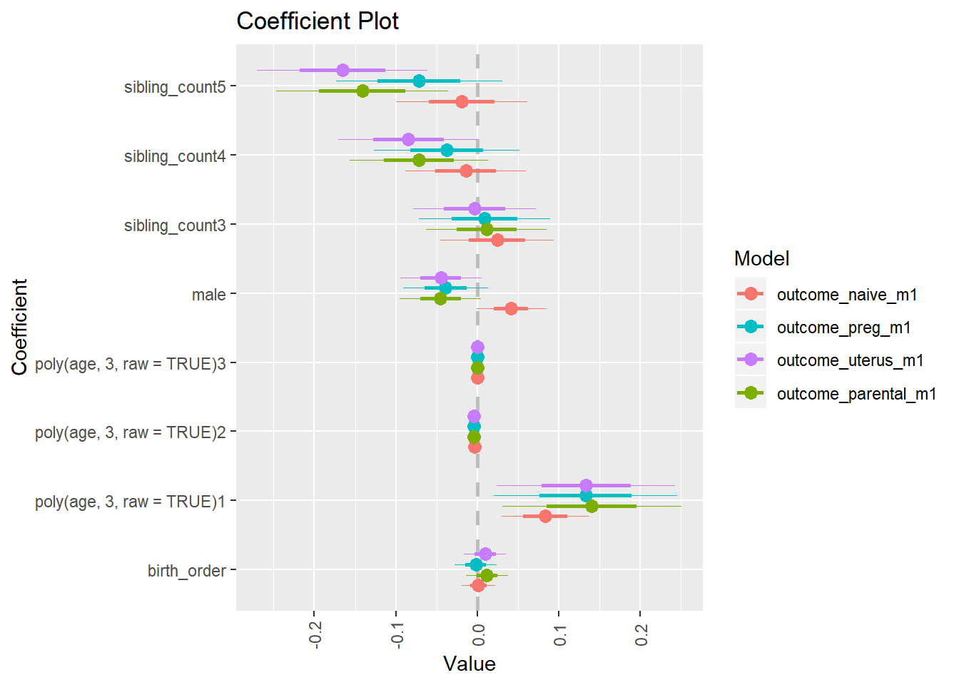
g-factor 2015 young
birthorder <- birthorder %>% mutate(outcome = g_factor_2015_young)
model = lmer(outcome ~ birth_order + poly(age, 3, raw = TRUE) + male + sibling_count + (1 | mother_pidlink),
                   data = birthorder)
compare_birthorder_specs(model)
Naive birth order
outcome_naive_m1 <- update(m2_birthorder_linear, data = birthorder %>%
                     mutate(sibling_count = sibling_count_naive_factor,
                            birth_order_nonlinear = birthorder_naive_factor,
                            birth_order = birthorder_naive,
                            count_birth_order = count_birthorder_naive) %>%
                     filter(sibling_count != "1"))
compare_models_markdown(outcome_naive_m1)
Basic Model
Model Summary
m1_covariates_only <- update(m2_birthorder_linear, formula = . ~ . - birth_order)
tidy(m1_covariates_only, conf.int = T, conf.level = 0.995)| effect | group | term | estimate | std.error | statistic | df | p.value | conf.low | conf.high |
|---|---|---|---|---|---|---|---|---|---|
| fixed | NA | (Intercept) | -3.083 | 0.1238 | -24.9 | 7824 | 8.961e-132 | -3.431 | -2.736 |
| fixed | NA | poly(age, 3, raw = TRUE)1 | 0.4532 | 0.023 | 19.7 | 7997 | 1.928e-84 | 0.3886 | 0.5177 |
| fixed | NA | poly(age, 3, raw = TRUE)2 | -0.01822 | 0.001326 | -13.75 | 8131 | 1.605e-42 | -0.02195 | -0.0145 |
| fixed | NA | poly(age, 3, raw = TRUE)3 | 0.0002241 | 0.00002419 | 9.264 | 8079 | 2.486e-20 | 0.0001562 | 0.000292 |
| fixed | NA | male | -0.008124 | 0.01933 | -0.4203 | 7346 | 0.6743 | -0.06238 | 0.04613 |
| fixed | NA | sibling_count3 | -0.03141 | 0.02829 | -1.11 | 5286 | 0.267 | -0.1108 | 0.04801 |
| fixed | NA | sibling_count4 | -0.1015 | 0.0319 | -3.182 | 4857 | 0.001474 | -0.1911 | -0.01195 |
| fixed | NA | sibling_count5 | -0.08078 | 0.03625 | -2.229 | 4457 | 0.02589 | -0.1825 | 0.02097 |
| ran_pars | mother_pidlink | sd__(Intercept) | 0.5378 | NA | NA | NA | NA | NA | NA |
| ran_pars | Residual | sd__Observation | 0.7408 | NA | NA | NA | NA | NA | NA |
Coefficient Plot
plot(allEffects(m1_covariates_only, confidence.level = 0.995))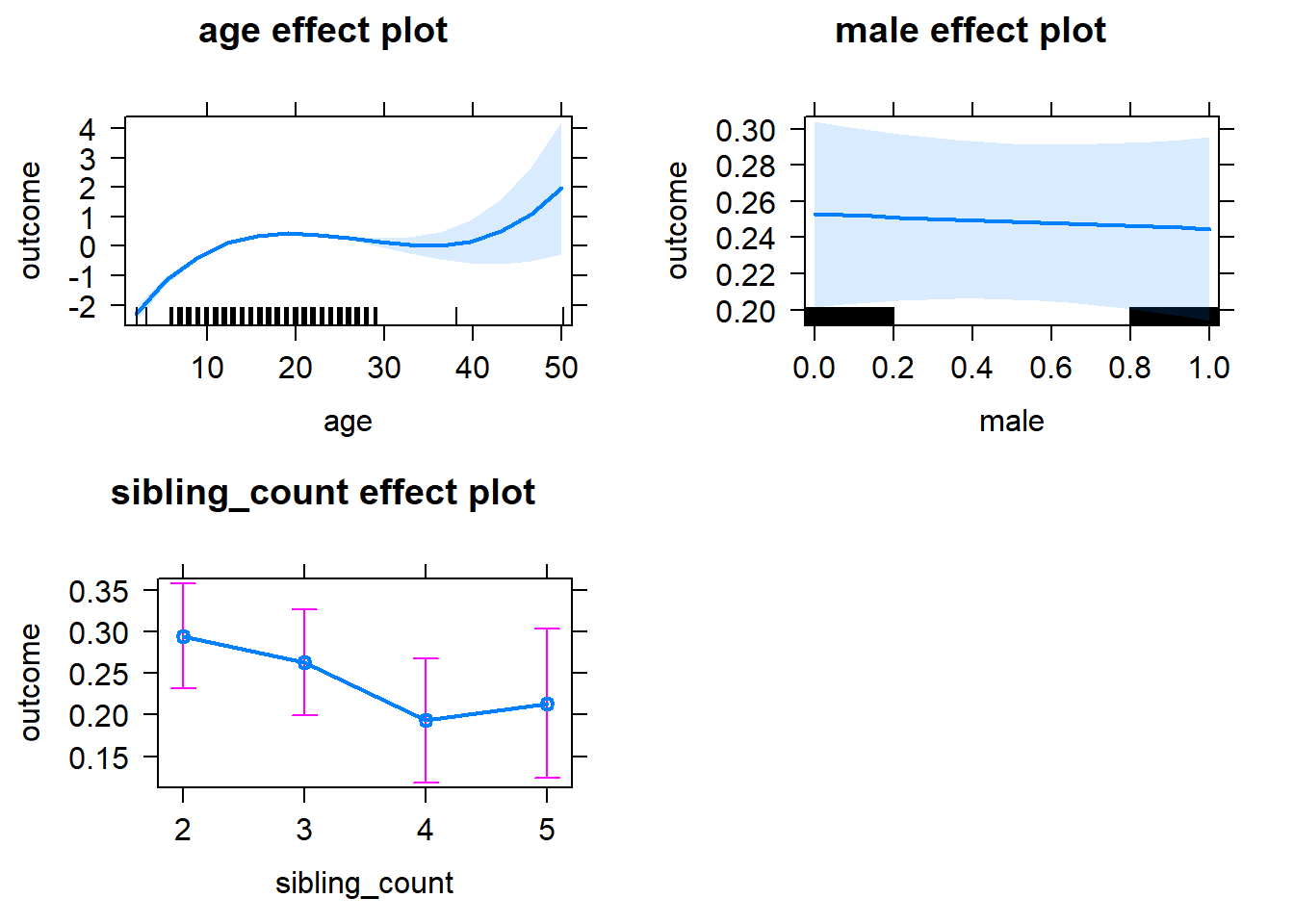
Add Birth Order Linear
Model Summary
tidy(m2_birthorder_linear, conf.int = T, conf.level = 0.995)| effect | group | term | estimate | std.error | statistic | df | p.value | conf.low | conf.high |
|---|---|---|---|---|---|---|---|---|---|
| fixed | NA | (Intercept) | -3.081 | 0.127 | -24.26 | 7931 | 1.93e-125 | -3.437 | -2.724 |
| fixed | NA | birth_order | -0.0009582 | 0.01068 | -0.08975 | 7577 | 0.9285 | -0.03093 | 0.02901 |
| fixed | NA | poly(age, 3, raw = TRUE)1 | 0.453 | 0.02306 | 19.65 | 8004 | 5.891e-84 | 0.3883 | 0.5178 |
| fixed | NA | poly(age, 3, raw = TRUE)2 | -0.01822 | 0.001327 | -13.74 | 8129 | 1.855e-42 | -0.02194 | -0.0145 |
| fixed | NA | poly(age, 3, raw = TRUE)3 | 0.0002241 | 0.00002419 | 9.261 | 8080 | 2.549e-20 | 0.0001562 | 0.000292 |
| fixed | NA | male | -0.008111 | 0.01933 | -0.4196 | 7346 | 0.6748 | -0.06237 | 0.04615 |
| fixed | NA | sibling_count3 | -0.03085 | 0.02896 | -1.066 | 5404 | 0.2867 | -0.1121 | 0.05043 |
| fixed | NA | sibling_count4 | -0.1002 | 0.03514 | -2.851 | 5264 | 0.004371 | -0.1988 | -0.001556 |
| fixed | NA | sibling_count5 | -0.07865 | 0.04336 | -1.814 | 5243 | 0.06976 | -0.2004 | 0.04307 |
| ran_pars | mother_pidlink | sd__(Intercept) | 0.5378 | NA | NA | NA | NA | NA | NA |
| ran_pars | Residual | sd__Observation | 0.7409 | NA | NA | NA | NA | NA | NA |
Coefficient Plot
plot_birthorder2(m2_birthorder_linear, separate = FALSE)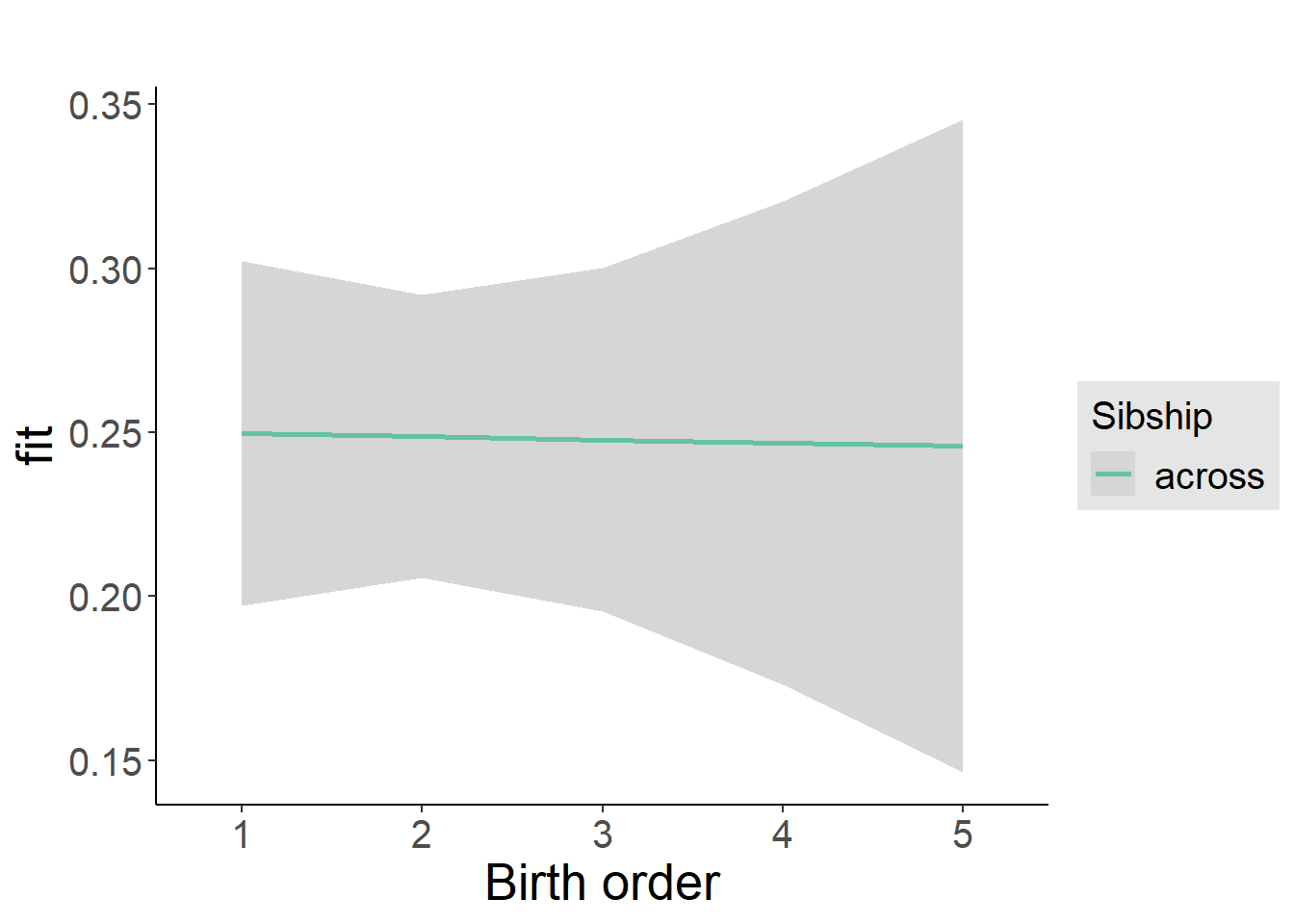
Add Birth Order Factor
Model Summary
m3_birthorder_nonlinear = update(m1_covariates_only, formula = . ~ . + birth_order_nonlinear)
tidy(m3_birthorder_nonlinear, conf.int = T, conf.level = 0.995)| effect | group | term | estimate | std.error | statistic | df | p.value | conf.low | conf.high |
|---|---|---|---|---|---|---|---|---|---|
| fixed | NA | (Intercept) | -3.093 | 0.1257 | -24.61 | 7926 | 6.766e-129 | -3.446 | -2.74 |
| fixed | NA | poly(age, 3, raw = TRUE)1 | 0.4541 | 0.02309 | 19.67 | 8015 | 3.81e-84 | 0.3893 | 0.5189 |
| fixed | NA | poly(age, 3, raw = TRUE)2 | -0.01827 | 0.001328 | -13.76 | 8128 | 1.326e-42 | -0.022 | -0.01454 |
| fixed | NA | poly(age, 3, raw = TRUE)3 | 0.0002247 | 0.00002421 | 9.282 | 8074 | 2.109e-20 | 0.0001567 | 0.0002926 |
| fixed | NA | male | -0.008347 | 0.01933 | -0.4318 | 7344 | 0.6659 | -0.06262 | 0.04592 |
| fixed | NA | sibling_count3 | -0.03815 | 0.02941 | -1.297 | 5626 | 0.1946 | -0.1207 | 0.0444 |
| fixed | NA | sibling_count4 | -0.1032 | 0.0358 | -2.881 | 5522 | 0.003977 | -0.2036 | -0.002654 |
| fixed | NA | sibling_count5 | -0.07188 | 0.04397 | -1.635 | 5375 | 0.1021 | -0.1953 | 0.05154 |
| fixed | NA | birth_order_nonlinear2 | 0.01223 | 0.02244 | 0.5448 | 5828 | 0.5859 | -0.05077 | 0.07523 |
| fixed | NA | birth_order_nonlinear3 | 0.02639 | 0.02963 | 0.8907 | 6575 | 0.3731 | -0.05679 | 0.1096 |
| fixed | NA | birth_order_nonlinear4 | -0.02156 | 0.0402 | -0.5363 | 6807 | 0.5918 | -0.1344 | 0.09128 |
| fixed | NA | birth_order_nonlinear5 | -0.02575 | 0.05839 | -0.441 | 6915 | 0.6592 | -0.1897 | 0.1382 |
| ran_pars | mother_pidlink | sd__(Intercept) | 0.538 | NA | NA | NA | NA | NA | NA |
| ran_pars | Residual | sd__Observation | 0.7408 | NA | NA | NA | NA | NA | NA |
Coefficient Plot
plot_birthorder(m3_birthorder_nonlinear, separate = FALSE)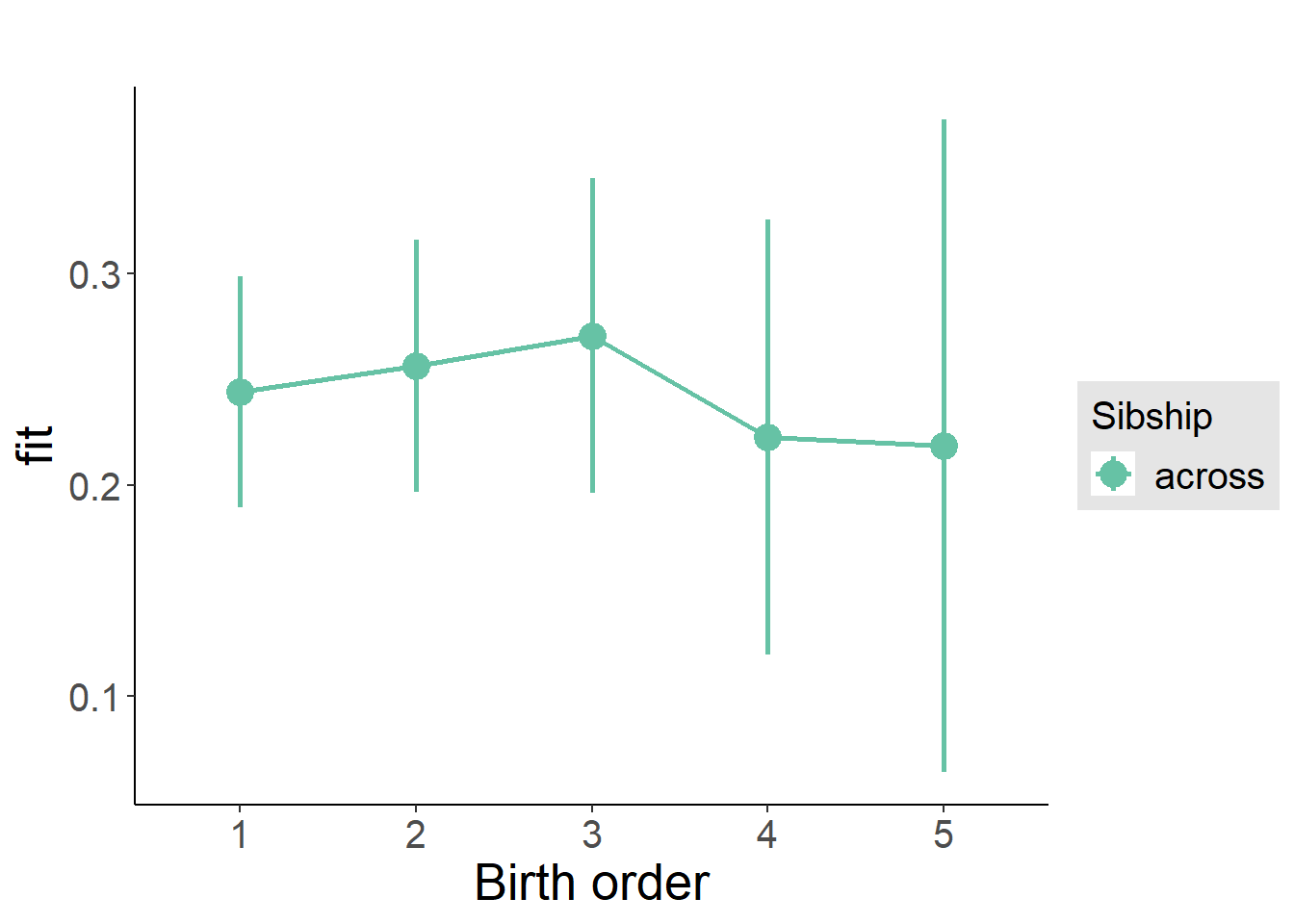
Add Interaction
Model Summary
m4_interaction = update(m3_birthorder_nonlinear, formula = . ~ . - birth_order_nonlinear - sibling_count + count_birth_order)
tidy(m4_interaction, conf.int = T, conf.level = 0.995)| effect | group | term | estimate | std.error | statistic | df | p.value | conf.low | conf.high |
|---|---|---|---|---|---|---|---|---|---|
| fixed | NA | (Intercept) | -3.097 | 0.1266 | -24.47 | 7944 | 1.478e-127 | -3.452 | -2.742 |
| fixed | NA | poly(age, 3, raw = TRUE)1 | 0.4554 | 0.02313 | 19.69 | 8020 | 2.404e-84 | 0.3905 | 0.5203 |
| fixed | NA | poly(age, 3, raw = TRUE)2 | -0.01835 | 0.001329 | -13.8 | 8122 | 7.39e-43 | -0.02208 | -0.01462 |
| fixed | NA | poly(age, 3, raw = TRUE)3 | 0.0002261 | 0.00002422 | 9.333 | 8068 | 1.309e-20 | 0.0001581 | 0.0002941 |
| fixed | NA | male | -0.008984 | 0.01933 | -0.4647 | 7340 | 0.6422 | -0.06326 | 0.04529 |
| fixed | NA | count_birth_order2/2 | 0.007872 | 0.03522 | 0.2235 | 6133 | 0.8232 | -0.091 | 0.1067 |
| fixed | NA | count_birth_order1/3 | -0.05798 | 0.03658 | -1.585 | 7989 | 0.113 | -0.1607 | 0.04471 |
| fixed | NA | count_birth_order2/3 | -0.03211 | 0.03721 | -0.8631 | 8067 | 0.3881 | -0.1366 | 0.07233 |
| fixed | NA | count_birth_order3/3 | 0.02493 | 0.04208 | 0.5925 | 8124 | 0.5536 | -0.09319 | 0.143 |
| fixed | NA | count_birth_order1/4 | -0.09505 | 0.05004 | -1.899 | 8115 | 0.05754 | -0.2355 | 0.04542 |
| fixed | NA | count_birth_order2/4 | -0.06273 | 0.04741 | -1.323 | 8113 | 0.1859 | -0.1958 | 0.07036 |
| fixed | NA | count_birth_order3/4 | -0.1402 | 0.0446 | -3.144 | 8124 | 0.00167 | -0.2654 | -0.01504 |
| fixed | NA | count_birth_order4/4 | -0.08802 | 0.04859 | -1.812 | 8099 | 0.07009 | -0.2244 | 0.04837 |
| fixed | NA | count_birth_order1/5 | -0.01007 | 0.06774 | -0.1487 | 7742 | 0.8818 | -0.2002 | 0.1801 |
| fixed | NA | count_birth_order2/5 | -0.09053 | 0.06435 | -1.407 | 7831 | 0.1595 | -0.2711 | 0.09009 |
| fixed | NA | count_birth_order3/5 | -0.005519 | 0.05823 | -0.09479 | 7995 | 0.9245 | -0.169 | 0.1579 |
| fixed | NA | count_birth_order4/5 | -0.1444 | 0.05474 | -2.639 | 8082 | 0.008339 | -0.2981 | 0.009217 |
| fixed | NA | count_birth_order5/5 | -0.0987 | 0.05428 | -1.818 | 8106 | 0.06903 | -0.2511 | 0.05366 |
| ran_pars | mother_pidlink | sd__(Intercept) | 0.538 | NA | NA | NA | NA | NA | NA |
| ran_pars | Residual | sd__Observation | 0.7406 | NA | NA | NA | NA | NA | NA |
Coefficient Plot
plot_birthorder(m4_interaction)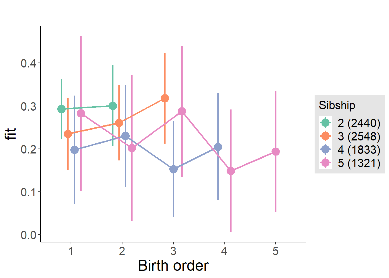
Model Comparison
###### Model 1 - Model 2
anova(m1_covariates_only, m2_birthorder_linear, m3_birthorder_nonlinear, m4_interaction)
## refitting model(s) with ML (instead of REML)| Df | AIC | BIC | logLik | deviance | Chisq | Chi Df | Pr(>Chisq) |
|---|---|---|---|---|---|---|---|
| 10 | 21276 | 21346 | -10628 | 21256 | NA | NA | NA |
| 11 | 21278 | 21355 | -10628 | 21256 | 0.008064 | 1 | 0.9284 |
| 14 | 21282 | 21380 | -10627 | 21254 | 2.199 | 3 | 0.5321 |
| 20 | 21284 | 21424 | -10622 | 21244 | 10.01 | 6 | 0.1242 |
Maternal birth order
outcome_uterus_m1 <- update(m2_birthorder_linear, data = birthorder %>%
                     mutate(sibling_count = sibling_count_uterus_alive_factor,
                            birth_order_nonlinear = birthorder_uterus_alive_factor,
                            birth_order = birthorder_uterus_alive,
                            count_birth_order = count_birthorder_uterus_alive) %>%
                     filter(sibling_count != "1"))
compare_models_markdown(outcome_uterus_m1)
Basic Model
Model Summary
m1_covariates_only <- update(m2_birthorder_linear, formula = . ~ . - birth_order)
tidy(m1_covariates_only, conf.int = T, conf.level = 0.995)| effect | group | term | estimate | std.error | statistic | df | p.value | conf.low | conf.high |
|---|---|---|---|---|---|---|---|---|---|
| fixed | NA | (Intercept) | -3.627 | 0.1999 | -18.15 | 6250 | 9.36e-72 | -4.188 | -3.066 |
| fixed | NA | poly(age, 3, raw = TRUE)1 | 0.5706 | 0.04194 | 13.61 | 6240 | 1.451e-41 | 0.4529 | 0.6884 |
| fixed | NA | poly(age, 3, raw = TRUE)2 | -0.02578 | 0.002715 | -9.497 | 6284 | 3.006e-21 | -0.0334 | -0.01816 |
| fixed | NA | poly(age, 3, raw = TRUE)3 | 0.0003777 | 0.00005446 | 6.935 | 6329 | 4.452e-12 | 0.0002248 | 0.0005306 |
| fixed | NA | male | -0.02086 | 0.02012 | -1.037 | 6918 | 0.2999 | -0.07734 | 0.03562 |
| fixed | NA | sibling_count3 | -0.0516 | 0.0273 | -1.89 | 4730 | 0.05883 | -0.1282 | 0.02504 |
| fixed | NA | sibling_count4 | -0.1156 | 0.0336 | -3.44 | 4168 | 0.0005881 | -0.2099 | -0.02126 |
| fixed | NA | sibling_count5 | -0.23 | 0.04319 | -5.327 | 3806 | 0.0000001059 | -0.3513 | -0.1088 |
| ran_pars | mother_pidlink | sd__(Intercept) | 0.5172 | NA | NA | NA | NA | NA | NA |
| ran_pars | Residual | sd__Observation | 0.7472 | NA | NA | NA | NA | NA | NA |
Coefficient Plot
plot(allEffects(m1_covariates_only, confidence.level = 0.995))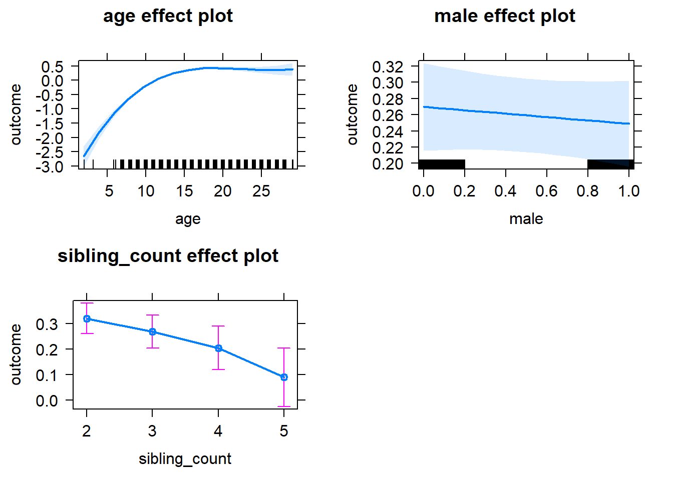
Add Birth Order Linear
Model Summary
tidy(m2_birthorder_linear, conf.int = T, conf.level = 0.995)| effect | group | term | estimate | std.error | statistic | df | p.value | conf.low | conf.high |
|---|---|---|---|---|---|---|---|---|---|
| fixed | NA | (Intercept) | -3.613 | 0.203 | -17.8 | 6425 | 3.321e-69 | -4.183 | -3.043 |
| fixed | NA | birth_order | -0.004797 | 0.01238 | -0.3876 | 7182 | 0.6983 | -0.03954 | 0.02994 |
| fixed | NA | poly(age, 3, raw = TRUE)1 | 0.5696 | 0.04202 | 13.56 | 6265 | 2.81e-41 | 0.4517 | 0.6876 |
| fixed | NA | poly(age, 3, raw = TRUE)2 | -0.02574 | 0.002716 | -9.477 | 6285 | 3.625e-21 | -0.03337 | -0.01812 |
| fixed | NA | poly(age, 3, raw = TRUE)3 | 0.0003773 | 0.00005448 | 6.925 | 6327 | 4.804e-12 | 0.0002243 | 0.0005302 |
| fixed | NA | male | -0.02076 | 0.02012 | -1.032 | 6919 | 0.3022 | -0.07725 | 0.03572 |
| fixed | NA | sibling_count3 | -0.04839 | 0.02853 | -1.696 | 4844 | 0.08993 | -0.1285 | 0.0317 |
| fixed | NA | sibling_count4 | -0.1084 | 0.03833 | -2.829 | 4626 | 0.004691 | -0.216 | -0.0008389 |
| fixed | NA | sibling_count5 | -0.2182 | 0.05292 | -4.123 | 4691 | 0.00003807 | -0.3667 | -0.06963 |
| ran_pars | mother_pidlink | sd__(Intercept) | 0.5171 | NA | NA | NA | NA | NA | NA |
| ran_pars | Residual | sd__Observation | 0.7473 | NA | NA | NA | NA | NA | NA |
Coefficient Plot
plot_birthorder2(m2_birthorder_linear, separate = FALSE)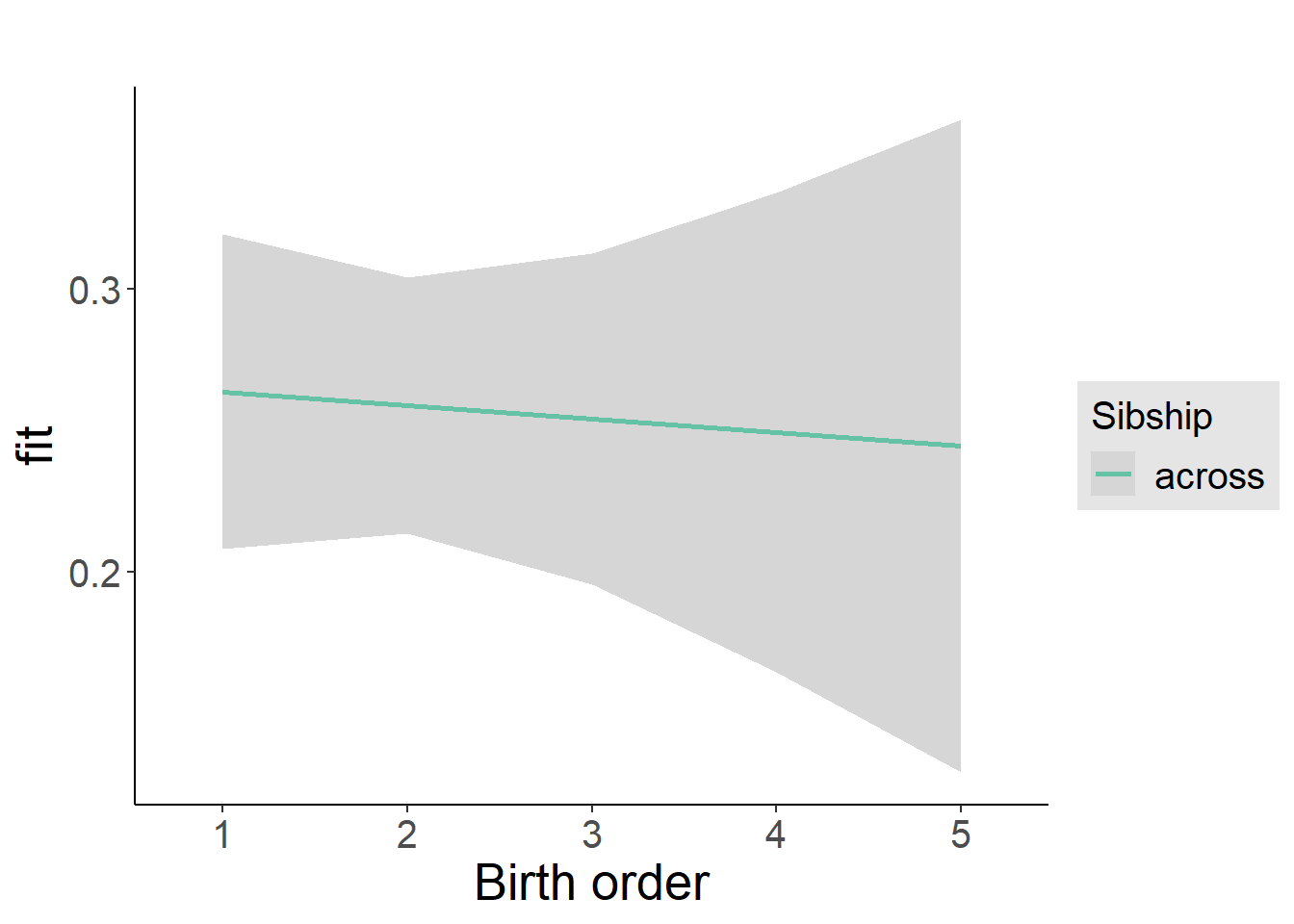
Add Birth Order Factor
Model Summary
m3_birthorder_nonlinear = update(m1_covariates_only, formula = . ~ . + birth_order_nonlinear)
tidy(m3_birthorder_nonlinear, conf.int = T, conf.level = 0.995)| effect | group | term | estimate | std.error | statistic | df | p.value | conf.low | conf.high |
|---|---|---|---|---|---|---|---|---|---|
| fixed | NA | (Intercept) | -3.628 | 0.2016 | -18 | 6374 | 1.117e-70 | -4.194 | -3.062 |
| fixed | NA | poly(age, 3, raw = TRUE)1 | 0.5702 | 0.04203 | 13.57 | 6269 | 2.428e-41 | 0.4522 | 0.6882 |
| fixed | NA | poly(age, 3, raw = TRUE)2 | -0.02575 | 0.002717 | -9.479 | 6286 | 3.566e-21 | -0.03338 | -0.01813 |
| fixed | NA | poly(age, 3, raw = TRUE)3 | 0.000377 | 0.00005449 | 6.918 | 6328 | 5.024e-12 | 0.000224 | 0.0005299 |
| fixed | NA | male | -0.02136 | 0.02013 | -1.061 | 6919 | 0.2887 | -0.07786 | 0.03514 |
| fixed | NA | sibling_count3 | -0.0557 | 0.0292 | -1.907 | 5130 | 0.05653 | -0.1377 | 0.02627 |
| fixed | NA | sibling_count4 | -0.1139 | 0.03924 | -2.904 | 4858 | 0.003706 | -0.2241 | -0.003786 |
| fixed | NA | sibling_count5 | -0.1914 | 0.05551 | -3.448 | 4961 | 0.0005684 | -0.3472 | -0.03561 |
| fixed | NA | birth_order_nonlinear2 | 0.009611 | 0.02281 | 0.4213 | 5364 | 0.6736 | -0.05443 | 0.07365 |
| fixed | NA | birth_order_nonlinear3 | 0.01457 | 0.03256 | 0.4476 | 6241 | 0.6544 | -0.07681 | 0.106 |
| fixed | NA | birth_order_nonlinear4 | -0.01329 | 0.04644 | -0.2862 | 6606 | 0.7748 | -0.1437 | 0.1171 |
| fixed | NA | birth_order_nonlinear5 | -0.1016 | 0.07323 | -1.388 | 6513 | 0.1652 | -0.3072 | 0.1039 |
| ran_pars | mother_pidlink | sd__(Intercept) | 0.5169 | NA | NA | NA | NA | NA | NA |
| ran_pars | Residual | sd__Observation | 0.7475 | NA | NA | NA | NA | NA | NA |
Coefficient Plot
plot_birthorder(m3_birthorder_nonlinear, separate = FALSE)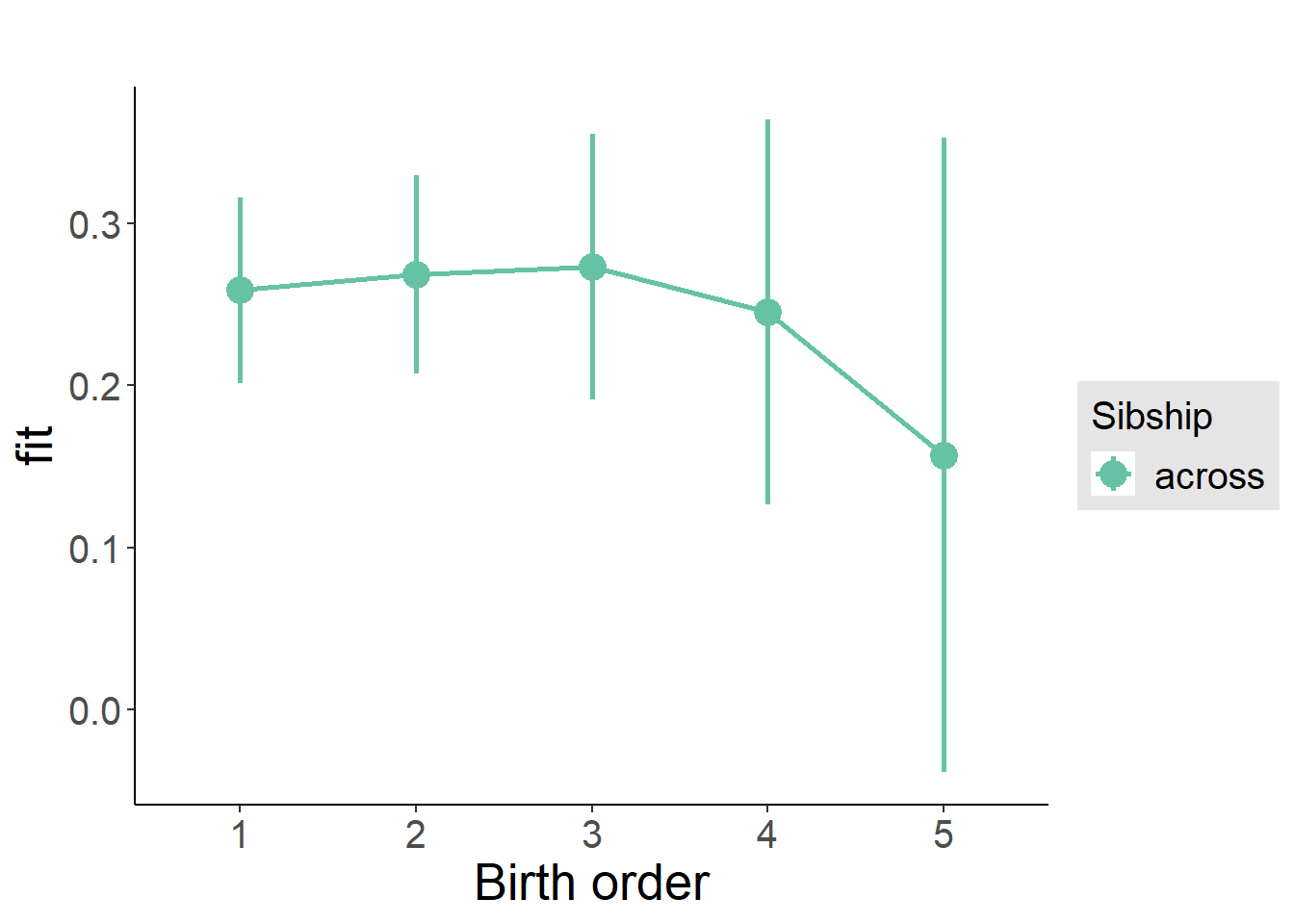
Add Interaction
Model Summary
m4_interaction = update(m3_birthorder_nonlinear, formula = . ~ . - birth_order_nonlinear - sibling_count + count_birth_order)
tidy(m4_interaction, conf.int = T, conf.level = 0.995)| effect | group | term | estimate | std.error | statistic | df | p.value | conf.low | conf.high |
|---|---|---|---|---|---|---|---|---|---|
| fixed | NA | (Intercept) | -3.639 | 0.2023 | -17.99 | 6396 | 1.16e-70 | -4.207 | -3.072 |
| fixed | NA | poly(age, 3, raw = TRUE)1 | 0.5723 | 0.04209 | 13.6 | 6276 | 1.621e-41 | 0.4541 | 0.6904 |
| fixed | NA | poly(age, 3, raw = TRUE)2 | -0.02591 | 0.00272 | -9.523 | 6287 | 2.34e-21 | -0.03354 | -0.01827 |
| fixed | NA | poly(age, 3, raw = TRUE)3 | 0.0003804 | 0.00005456 | 6.972 | 6324 | 3.445e-12 | 0.0002272 | 0.0005335 |
| fixed | NA | male | -0.02073 | 0.02013 | -1.03 | 6905 | 0.3033 | -0.07724 | 0.03579 |
| fixed | NA | count_birth_order2/2 | 0.02002 | 0.03173 | 0.631 | 5817 | 0.5281 | -0.06905 | 0.1091 |
| fixed | NA | count_birth_order1/3 | -0.05851 | 0.03768 | -1.553 | 7465 | 0.1206 | -0.1643 | 0.04727 |
| fixed | NA | count_birth_order2/3 | -0.05422 | 0.03619 | -1.498 | 7477 | 0.1342 | -0.1558 | 0.04738 |
| fixed | NA | count_birth_order3/3 | -0.01434 | 0.0396 | -0.3621 | 7506 | 0.7173 | -0.1255 | 0.09681 |
| fixed | NA | count_birth_order1/4 | -0.06173 | 0.05925 | -1.042 | 7365 | 0.2975 | -0.2281 | 0.1046 |
| fixed | NA | count_birth_order2/4 | -0.09877 | 0.05204 | -1.898 | 7489 | 0.05775 | -0.2448 | 0.04731 |
| fixed | NA | count_birth_order3/4 | -0.1626 | 0.04964 | -3.275 | 7490 | 0.001061 | -0.3019 | -0.02324 |
| fixed | NA | count_birth_order4/4 | -0.09257 | 0.04919 | -1.882 | 7510 | 0.0599 | -0.2307 | 0.04552 |
| fixed | NA | count_birth_order1/5 | -0.195 | 0.1027 | -1.898 | 6363 | 0.0577 | -0.4832 | 0.09333 |
| fixed | NA | count_birth_order2/5 | -0.1403 | 0.09161 | -1.531 | 6767 | 0.1258 | -0.3974 | 0.1169 |
| fixed | NA | count_birth_order3/5 | -0.09425 | 0.07768 | -1.213 | 7189 | 0.225 | -0.3123 | 0.1238 |
| fixed | NA | count_birth_order4/5 | -0.2587 | 0.06447 | -4.012 | 7496 | 0.00006081 | -0.4396 | -0.07769 |
| fixed | NA | count_birth_order5/5 | -0.2905 | 0.06257 | -4.642 | 7510 | 0.000003505 | -0.4661 | -0.1148 |
| ran_pars | mother_pidlink | sd__(Intercept) | 0.517 | NA | NA | NA | NA | NA | NA |
| ran_pars | Residual | sd__Observation | 0.7473 | NA | NA | NA | NA | NA | NA |
Coefficient Plot
plot_birthorder(m4_interaction)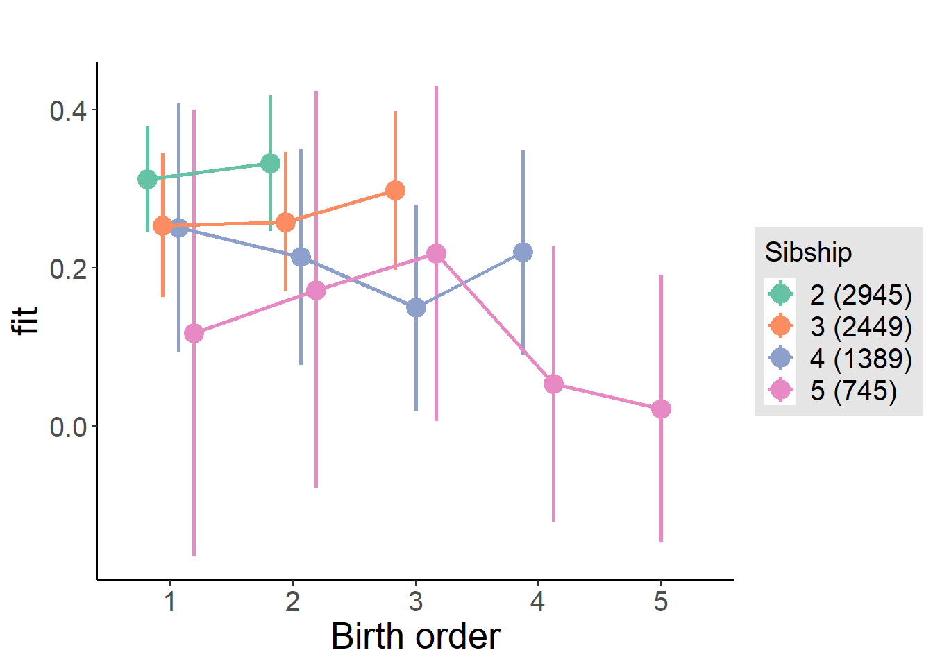
Model Comparison
###### Model 1 - Model 2
anova(m1_covariates_only, m2_birthorder_linear, m3_birthorder_nonlinear, m4_interaction)
## refitting model(s) with ML (instead of REML)| Df | AIC | BIC | logLik | deviance | Chisq | Chi Df | Pr(>Chisq) |
|---|---|---|---|---|---|---|---|
| 10 | 19620 | 19690 | -9800 | 19600 | NA | NA | NA |
| 11 | 19622 | 19698 | -9800 | 19600 | 0.1506 | 1 | 0.6979 |
| 14 | 19626 | 19723 | -9799 | 19598 | 2.709 | 3 | 0.4387 |
| 20 | 19630 | 19768 | -9795 | 19590 | 7.688 | 6 | 0.2619 |
Maternal pregnancy order
outcome_preg_m1 <- update(m2_birthorder_linear, data = birthorder %>%
  mutate(sibling_count = sibling_count_uterus_preg_factor,
         birth_order_nonlinear = birthorder_uterus_preg_factor,
         birth_order = birthorder_uterus_preg,
         count_birth_order = count_birthorder_uterus_preg
         ) %>%
    filter(sibling_count != "1"))
compare_models_markdown(outcome_preg_m1)
Basic Model
Model Summary
m1_covariates_only <- update(m2_birthorder_linear, formula = . ~ . - birth_order)
tidy(m1_covariates_only, conf.int = T, conf.level = 0.995)| effect | group | term | estimate | std.error | statistic | df | p.value | conf.low | conf.high |
|---|---|---|---|---|---|---|---|---|---|
| fixed | NA | (Intercept) | -3.666 | 0.2047 | -17.91 | 5929 | 7.22e-70 | -4.241 | -3.091 |
| fixed | NA | poly(age, 3, raw = TRUE)1 | 0.581 | 0.0431 | 13.48 | 5907 | 7.969e-41 | 0.46 | 0.702 |
| fixed | NA | poly(age, 3, raw = TRUE)2 | -0.02675 | 0.002797 | -9.563 | 5944 | 1.629e-21 | -0.0346 | -0.0189 |
| fixed | NA | poly(age, 3, raw = TRUE)3 | 0.0004002 | 0.00005625 | 7.115 | 5980 | 1.247e-12 | 0.0002423 | 0.0005581 |
| fixed | NA | male | -0.02033 | 0.02061 | -0.9865 | 6546 | 0.3239 | -0.07818 | 0.03752 |
| fixed | NA | sibling_count3 | -0.02948 | 0.02861 | -1.03 | 4669 | 0.3029 | -0.1098 | 0.05084 |
| fixed | NA | sibling_count4 | -0.07251 | 0.03375 | -2.148 | 4252 | 0.03175 | -0.1672 | 0.02223 |
| fixed | NA | sibling_count5 | -0.08763 | 0.03965 | -2.21 | 3957 | 0.02715 | -0.1989 | 0.02367 |
| ran_pars | mother_pidlink | sd__(Intercept) | 0.5228 | NA | NA | NA | NA | NA | NA |
| ran_pars | Residual | sd__Observation | 0.7443 | NA | NA | NA | NA | NA | NA |
Coefficient Plot
plot(allEffects(m1_covariates_only, confidence.level = 0.995))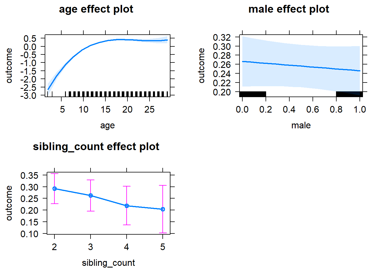
Add Birth Order Linear
Model Summary
tidy(m2_birthorder_linear, conf.int = T, conf.level = 0.995)| effect | group | term | estimate | std.error | statistic | df | p.value | conf.low | conf.high |
|---|---|---|---|---|---|---|---|---|---|
| fixed | NA | (Intercept) | -3.62 | 0.2077 | -17.43 | 6080 | 2.026e-66 | -4.203 | -3.037 |
| fixed | NA | birth_order | -0.01575 | 0.01201 | -1.311 | 6894 | 0.1898 | -0.04948 | 0.01797 |
| fixed | NA | poly(age, 3, raw = TRUE)1 | 0.5775 | 0.04318 | 13.38 | 5929 | 3.217e-40 | 0.4563 | 0.6987 |
| fixed | NA | poly(age, 3, raw = TRUE)2 | -0.02661 | 0.002799 | -9.507 | 5944 | 2.777e-21 | -0.03447 | -0.01875 |
| fixed | NA | poly(age, 3, raw = TRUE)3 | 0.0003983 | 0.00005627 | 7.078 | 5978 | 1.636e-12 | 0.0002403 | 0.0005562 |
| fixed | NA | male | -0.01994 | 0.02061 | -0.9675 | 6548 | 0.3333 | -0.0778 | 0.03792 |
| fixed | NA | sibling_count3 | -0.0196 | 0.02958 | -0.6627 | 4780 | 0.5076 | -0.1026 | 0.06343 |
| fixed | NA | sibling_count4 | -0.05019 | 0.03779 | -1.328 | 4668 | 0.1842 | -0.1563 | 0.05589 |
| fixed | NA | sibling_count5 | -0.05252 | 0.04783 | -1.098 | 4743 | 0.2722 | -0.1868 | 0.08172 |
| ran_pars | mother_pidlink | sd__(Intercept) | 0.5223 | NA | NA | NA | NA | NA | NA |
| ran_pars | Residual | sd__Observation | 0.7445 | NA | NA | NA | NA | NA | NA |
Coefficient Plot
plot_birthorder2(m2_birthorder_linear, separate = FALSE)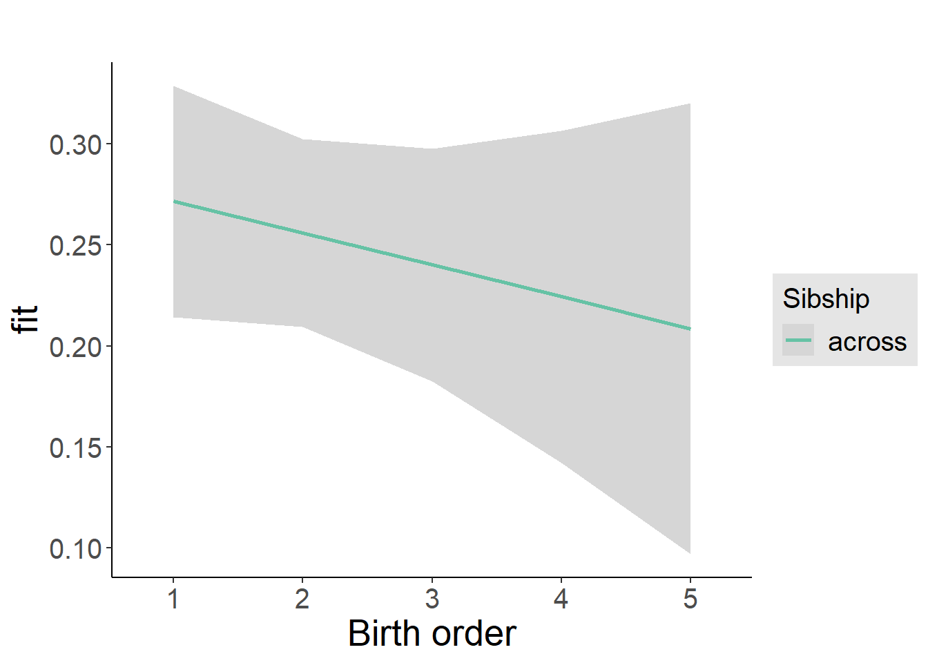
Add Birth Order Factor
Model Summary
m3_birthorder_nonlinear = update(m1_covariates_only, formula = . ~ . + birth_order_nonlinear)
tidy(m3_birthorder_nonlinear, conf.int = T, conf.level = 0.995)| effect | group | term | estimate | std.error | statistic | df | p.value | conf.low | conf.high |
|---|---|---|---|---|---|---|---|---|---|
| fixed | NA | (Intercept) | -3.644 | 0.2064 | -17.65 | 6037 | 4.893e-68 | -4.224 | -3.065 |
| fixed | NA | poly(age, 3, raw = TRUE)1 | 0.5779 | 0.0432 | 13.38 | 5933 | 3.099e-40 | 0.4566 | 0.6991 |
| fixed | NA | poly(age, 3, raw = TRUE)2 | -0.0266 | 0.0028 | -9.5 | 5946 | 2.979e-21 | -0.03446 | -0.01874 |
| fixed | NA | poly(age, 3, raw = TRUE)3 | 0.0003975 | 0.00005629 | 7.062 | 5980 | 1.829e-12 | 0.0002395 | 0.0005555 |
| fixed | NA | male | -0.02051 | 0.02061 | -0.9948 | 6546 | 0.3199 | -0.07837 | 0.03736 |
| fixed | NA | sibling_count3 | -0.02767 | 0.03024 | -0.9153 | 5034 | 0.3601 | -0.1125 | 0.0572 |
| fixed | NA | sibling_count4 | -0.05929 | 0.03869 | -1.533 | 4893 | 0.1254 | -0.1679 | 0.04931 |
| fixed | NA | sibling_count5 | -0.03552 | 0.04908 | -0.7236 | 4898 | 0.4693 | -0.1733 | 0.1023 |
| fixed | NA | birth_order_nonlinear2 | -0.003182 | 0.02367 | -0.1344 | 5065 | 0.8931 | -0.06961 | 0.06325 |
| fixed | NA | birth_order_nonlinear3 | -0.003502 | 0.03252 | -0.1077 | 6018 | 0.9142 | -0.0948 | 0.08779 |
| fixed | NA | birth_order_nonlinear4 | -0.03829 | 0.0452 | -0.847 | 6358 | 0.397 | -0.1652 | 0.08859 |
| fixed | NA | birth_order_nonlinear5 | -0.139 | 0.06737 | -2.062 | 6301 | 0.03921 | -0.3281 | 0.05016 |
| ran_pars | mother_pidlink | sd__(Intercept) | 0.5222 | NA | NA | NA | NA | NA | NA |
| ran_pars | Residual | sd__Observation | 0.7446 | NA | NA | NA | NA | NA | NA |
Coefficient Plot
plot_birthorder(m3_birthorder_nonlinear, separate = FALSE)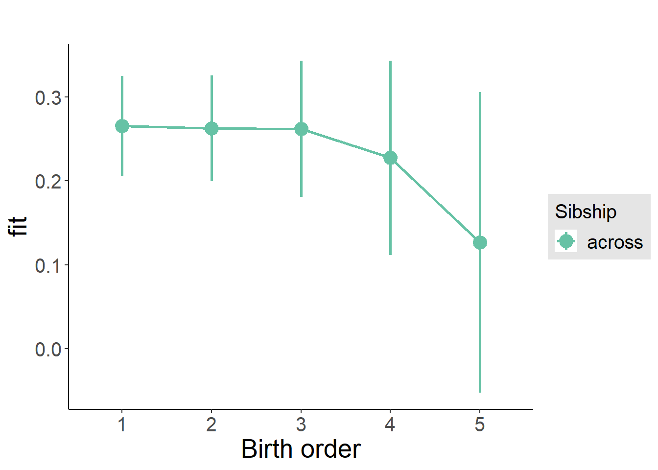
Add Interaction
Model Summary
m4_interaction = update(m3_birthorder_nonlinear, formula = . ~ . - birth_order_nonlinear - sibling_count + count_birth_order)
tidy(m4_interaction, conf.int = T, conf.level = 0.995)| effect | group | term | estimate | std.error | statistic | df | p.value | conf.low | conf.high |
|---|---|---|---|---|---|---|---|---|---|
| fixed | NA | (Intercept) | -3.655 | 0.2073 | -17.63 | 6053 | 7.171e-68 | -4.237 | -3.073 |
| fixed | NA | poly(age, 3, raw = TRUE)1 | 0.5806 | 0.04327 | 13.42 | 5939 | 1.821e-40 | 0.4591 | 0.702 |
| fixed | NA | poly(age, 3, raw = TRUE)2 | -0.02681 | 0.002804 | -9.559 | 5946 | 1.689e-21 | -0.03468 | -0.01894 |
| fixed | NA | poly(age, 3, raw = TRUE)3 | 0.0004023 | 0.00005638 | 7.136 | 5975 | 1.076e-12 | 0.000244 | 0.0005606 |
| fixed | NA | male | -0.01985 | 0.02062 | -0.9629 | 6535 | 0.3357 | -0.07773 | 0.03802 |
| fixed | NA | count_birth_order2/2 | -0.002972 | 0.03461 | -0.08587 | 5441 | 0.9316 | -0.1001 | 0.09417 |
| fixed | NA | count_birth_order1/3 | -0.03706 | 0.03898 | -0.9505 | 7118 | 0.3419 | -0.1465 | 0.07237 |
| fixed | NA | count_birth_order2/3 | -0.03475 | 0.03807 | -0.9128 | 7133 | 0.3614 | -0.1416 | 0.07212 |
| fixed | NA | count_birth_order3/3 | -0.01403 | 0.04172 | -0.3362 | 7149 | 0.7368 | -0.1311 | 0.1031 |
| fixed | NA | count_birth_order1/4 | -0.08157 | 0.05792 | -1.408 | 7056 | 0.1591 | -0.2441 | 0.08101 |
| fixed | NA | count_birth_order2/4 | -0.05563 | 0.052 | -1.07 | 7115 | 0.2847 | -0.2016 | 0.09033 |
| fixed | NA | count_birth_order3/4 | -0.1043 | 0.04975 | -2.096 | 7128 | 0.03614 | -0.2439 | 0.03539 |
| fixed | NA | count_birth_order4/4 | -0.04947 | 0.05034 | -0.9829 | 7153 | 0.3257 | -0.1908 | 0.09182 |
| fixed | NA | count_birth_order1/5 | 0.07996 | 0.08392 | 0.9528 | 6471 | 0.3407 | -0.1556 | 0.3155 |
| fixed | NA | count_birth_order2/5 | -0.03529 | 0.07519 | -0.4693 | 6782 | 0.6389 | -0.2464 | 0.1758 |
| fixed | NA | count_birth_order3/5 | -0.006645 | 0.06755 | -0.09837 | 6939 | 0.9216 | -0.1963 | 0.183 |
| fixed | NA | count_birth_order4/5 | -0.1521 | 0.06228 | -2.443 | 7054 | 0.01459 | -0.327 | 0.02268 |
| fixed | NA | count_birth_order5/5 | -0.1769 | 0.06004 | -2.947 | 7144 | 0.00322 | -0.3454 | -0.008396 |
| ran_pars | mother_pidlink | sd__(Intercept) | 0.5225 | NA | NA | NA | NA | NA | NA |
| ran_pars | Residual | sd__Observation | 0.7443 | NA | NA | NA | NA | NA | NA |
Coefficient Plot
plot_birthorder(m4_interaction)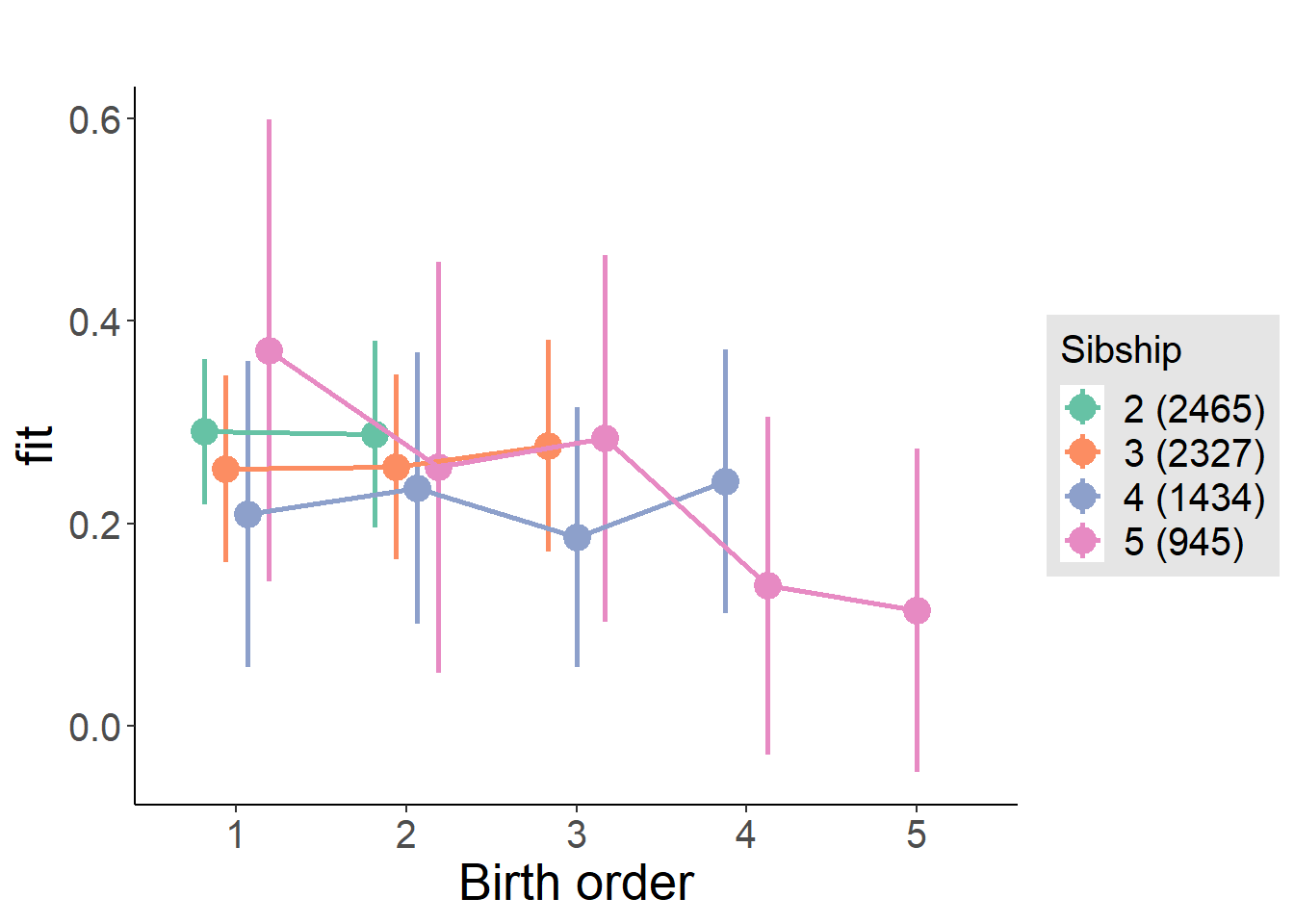
Model Comparison
###### Model 1 - Model 2
anova(m1_covariates_only, m2_birthorder_linear, m3_birthorder_nonlinear, m4_interaction)
## refitting model(s) with ML (instead of REML)| Df | AIC | BIC | logLik | deviance | Chisq | Chi Df | Pr(>Chisq) |
|---|---|---|---|---|---|---|---|
| 10 | 18703 | 18772 | -9342 | 18683 | NA | NA | NA |
| 11 | 18703 | 18779 | -9341 | 18681 | 1.722 | 1 | 0.1895 |
| 14 | 18706 | 18803 | -9339 | 18678 | 2.938 | 3 | 0.4013 |
| 20 | 18711 | 18848 | -9335 | 18671 | 7.677 | 6 | 0.2627 |
Parental full sibling order
outcome_parental_m1 <- update(m2_birthorder_linear, data = birthorder %>%
  mutate(sibling_count = sibling_count_genes_factor,
         birth_order_nonlinear = birthorder_genes_factor,
         birth_order = birthorder_genes,
         count_birth_order = count_birthorder_genes
         ) %>%
      filter(sibling_count != "1"))
compare_models_markdown(outcome_parental_m1)
Basic Model
Model Summary
m1_covariates_only <- update(m2_birthorder_linear, formula = . ~ . - birth_order)
tidy(m1_covariates_only, conf.int = T, conf.level = 0.995)| effect | group | term | estimate | std.error | statistic | df | p.value | conf.low | conf.high |
|---|---|---|---|---|---|---|---|---|---|
| fixed | NA | (Intercept) | -3.602 | 0.2007 | -17.95 | 6146 | 3.013e-70 | -4.166 | -3.039 |
| fixed | NA | poly(age, 3, raw = TRUE)1 | 0.565 | 0.0421 | 13.42 | 6145 | 1.65e-40 | 0.4469 | 0.6832 |
| fixed | NA | poly(age, 3, raw = TRUE)2 | -0.02542 | 0.002722 | -9.337 | 6197 | 1.35e-20 | -0.03306 | -0.01778 |
| fixed | NA | poly(age, 3, raw = TRUE)3 | 0.0003703 | 0.00005457 | 6.785 | 6249 | 0.00000000001265 | 0.0002171 | 0.0005235 |
| fixed | NA | male | -0.02573 | 0.02023 | -1.272 | 6788 | 0.2034 | -0.08252 | 0.03105 |
| fixed | NA | sibling_count3 | -0.044 | 0.02736 | -1.608 | 4649 | 0.1078 | -0.1208 | 0.0328 |
| fixed | NA | sibling_count4 | -0.1002 | 0.03395 | -2.951 | 4083 | 0.003184 | -0.1955 | -0.004893 |
| fixed | NA | sibling_count5 | -0.2183 | 0.04499 | -4.852 | 3743 | 0.000001274 | -0.3446 | -0.09199 |
| ran_pars | mother_pidlink | sd__(Intercept) | 0.5175 | NA | NA | NA | NA | NA | NA |
| ran_pars | Residual | sd__Observation | 0.7437 | NA | NA | NA | NA | NA | NA |
Coefficient Plot
plot(allEffects(m1_covariates_only, confidence.level = 0.995))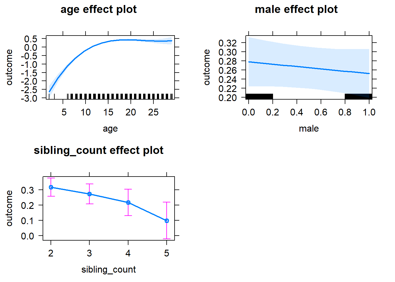
Add Birth Order Linear
Model Summary
tidy(m2_birthorder_linear, conf.int = T, conf.level = 0.995)| effect | group | term | estimate | std.error | statistic | df | p.value | conf.low | conf.high |
|---|---|---|---|---|---|---|---|---|---|
| fixed | NA | (Intercept) | -3.592 | 0.204 | -17.61 | 6317 | 8.329e-68 | -4.165 | -3.02 |
| fixed | NA | birth_order | -0.003464 | 0.01251 | -0.2769 | 7002 | 0.7818 | -0.03857 | 0.03164 |
| fixed | NA | poly(age, 3, raw = TRUE)1 | 0.5643 | 0.04218 | 13.38 | 6171 | 2.999e-40 | 0.4459 | 0.6827 |
| fixed | NA | poly(age, 3, raw = TRUE)2 | -0.02539 | 0.002724 | -9.32 | 6197 | 1.588e-20 | -0.03304 | -0.01774 |
| fixed | NA | poly(age, 3, raw = TRUE)3 | 0.0003699 | 0.00005459 | 6.776 | 6246 | 0.00000000001349 | 0.0002167 | 0.0005232 |
| fixed | NA | male | -0.02567 | 0.02023 | -1.269 | 6789 | 0.2045 | -0.08247 | 0.03112 |
| fixed | NA | sibling_count3 | -0.0417 | 0.02859 | -1.458 | 4767 | 0.1448 | -0.122 | 0.03856 |
| fixed | NA | sibling_count4 | -0.09507 | 0.03867 | -2.459 | 4555 | 0.01398 | -0.2036 | 0.01347 |
| fixed | NA | sibling_count5 | -0.2099 | 0.05425 | -3.868 | 4573 | 0.000111 | -0.3622 | -0.05759 |
| ran_pars | mother_pidlink | sd__(Intercept) | 0.5175 | NA | NA | NA | NA | NA | NA |
| ran_pars | Residual | sd__Observation | 0.7438 | NA | NA | NA | NA | NA | NA |
Coefficient Plot
plot_birthorder2(m2_birthorder_linear, separate = FALSE)
Add Birth Order Factor
Model Summary
m3_birthorder_nonlinear = update(m1_covariates_only, formula = . ~ . + birth_order_nonlinear)
tidy(m3_birthorder_nonlinear, conf.int = T, conf.level = 0.995)| effect | group | term | estimate | std.error | statistic | df | p.value | conf.low | conf.high |
|---|---|---|---|---|---|---|---|---|---|
| fixed | NA | (Intercept) | -3.603 | 0.2025 | -17.79 | 6270 | 3.98e-69 | -4.171 | -3.034 |
| fixed | NA | poly(age, 3, raw = TRUE)1 | 0.5644 | 0.0422 | 13.38 | 6176 | 3.054e-40 | 0.446 | 0.6829 |
| fixed | NA | poly(age, 3, raw = TRUE)2 | -0.02538 | 0.002725 | -9.312 | 6200 | 1.703e-20 | -0.03303 | -0.01773 |
| fixed | NA | poly(age, 3, raw = TRUE)3 | 0.0003693 | 0.00005461 | 6.763 | 6248 | 0.00000000001478 | 0.000216 | 0.0005226 |
| fixed | NA | male | -0.026 | 0.02024 | -1.285 | 6788 | 0.199 | -0.08281 | 0.03081 |
| fixed | NA | sibling_count3 | -0.04394 | 0.02925 | -1.502 | 5047 | 0.1331 | -0.1261 | 0.03817 |
| fixed | NA | sibling_count4 | -0.09961 | 0.03959 | -2.516 | 4794 | 0.0119 | -0.2107 | 0.01152 |
| fixed | NA | sibling_count5 | -0.188 | 0.05722 | -3.286 | 4832 | 0.001022 | -0.3486 | -0.02742 |
| fixed | NA | birth_order_nonlinear2 | 0.01017 | 0.02277 | 0.4466 | 5267 | 0.6552 | -0.05374 | 0.07408 |
| fixed | NA | birth_order_nonlinear3 | 0.0002027 | 0.0327 | 0.006198 | 6080 | 0.9951 | -0.09158 | 0.09198 |
| fixed | NA | birth_order_nonlinear4 | 0.002949 | 0.04722 | 0.06245 | 6395 | 0.9502 | -0.1296 | 0.1355 |
| fixed | NA | birth_order_nonlinear5 | -0.08493 | 0.07715 | -1.101 | 6452 | 0.271 | -0.3015 | 0.1316 |
| ran_pars | mother_pidlink | sd__(Intercept) | 0.517 | NA | NA | NA | NA | NA | NA |
| ran_pars | Residual | sd__Observation | 0.7441 | NA | NA | NA | NA | NA | NA |
Coefficient Plot
plot_birthorder(m3_birthorder_nonlinear, separate = FALSE)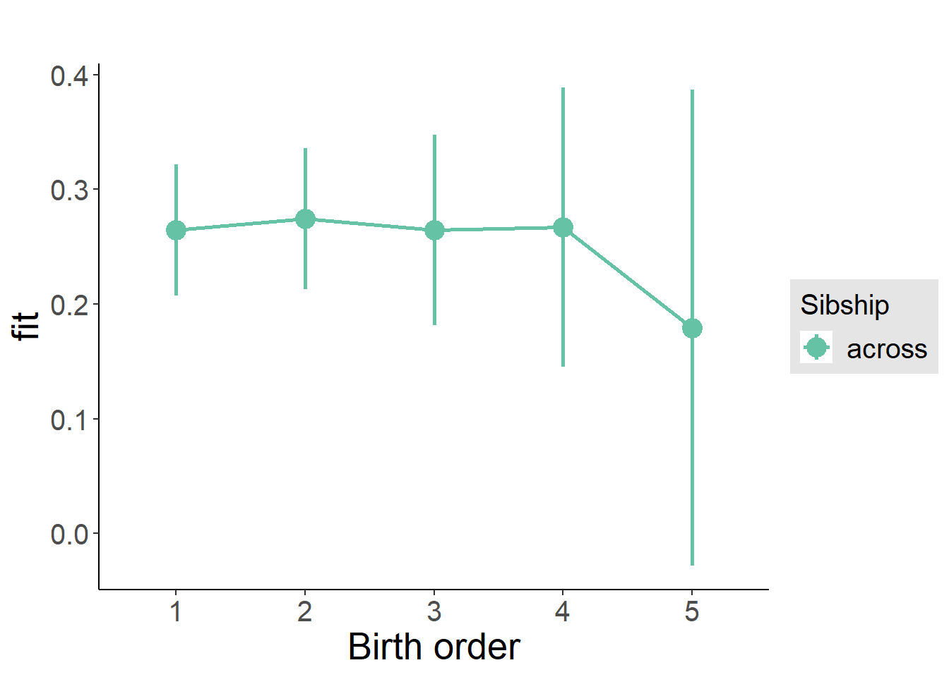
Add Interaction
Model Summary
m4_interaction = update(m3_birthorder_nonlinear, formula = . ~ . - birth_order_nonlinear - sibling_count + count_birth_order)
tidy(m4_interaction, conf.int = T, conf.level = 0.995)| effect | group | term | estimate | std.error | statistic | df | p.value | conf.low | conf.high |
|---|---|---|---|---|---|---|---|---|---|
| fixed | NA | (Intercept) | -3.607 | 0.2031 | -17.76 | 6289 | 7.159e-69 | -4.177 | -3.037 |
| fixed | NA | poly(age, 3, raw = TRUE)1 | 0.565 | 0.04225 | 13.37 | 6181 | 3.153e-40 | 0.4464 | 0.6836 |
| fixed | NA | poly(age, 3, raw = TRUE)2 | -0.02543 | 0.002729 | -9.32 | 6199 | 1.581e-20 | -0.03309 | -0.01777 |
| fixed | NA | poly(age, 3, raw = TRUE)3 | 0.0003706 | 0.00005467 | 6.778 | 6243 | 0.0000000000133 | 0.0002171 | 0.000524 |
| fixed | NA | male | -0.02521 | 0.02024 | -1.245 | 6778 | 0.213 | -0.08203 | 0.03161 |
| fixed | NA | count_birth_order2/2 | 0.0168 | 0.03136 | 0.5358 | 5661 | 0.5921 | -0.07123 | 0.1048 |
| fixed | NA | count_birth_order1/3 | -0.04745 | 0.03781 | -1.255 | 7329 | 0.2095 | -0.1536 | 0.05869 |
| fixed | NA | count_birth_order2/3 | -0.0408 | 0.03627 | -1.125 | 7338 | 0.2607 | -0.1426 | 0.06101 |
| fixed | NA | count_birth_order3/3 | -0.02223 | 0.03973 | -0.5595 | 7368 | 0.5759 | -0.1338 | 0.0893 |
| fixed | NA | count_birth_order1/4 | -0.06359 | 0.05955 | -1.068 | 7242 | 0.2857 | -0.2307 | 0.1036 |
| fixed | NA | count_birth_order2/4 | -0.08109 | 0.05266 | -1.54 | 7347 | 0.1236 | -0.2289 | 0.06673 |
| fixed | NA | count_birth_order3/4 | -0.1601 | 0.04996 | -3.205 | 7353 | 0.001358 | -0.3003 | -0.01987 |
| fixed | NA | count_birth_order4/4 | -0.06132 | 0.04983 | -1.231 | 7371 | 0.2185 | -0.2012 | 0.07855 |
| fixed | NA | count_birth_order1/5 | -0.1793 | 0.1026 | -1.748 | 6417 | 0.08056 | -0.4672 | 0.1087 |
| fixed | NA | count_birth_order2/5 | -0.1509 | 0.09813 | -1.537 | 6543 | 0.1242 | -0.4263 | 0.1246 |
| fixed | NA | count_birth_order3/5 | -0.09533 | 0.07971 | -1.196 | 7119 | 0.2317 | -0.3191 | 0.1284 |
| fixed | NA | count_birth_order4/5 | -0.2489 | 0.06774 | -3.674 | 7353 | 0.0002405 | -0.439 | -0.05872 |
| fixed | NA | count_birth_order5/5 | -0.2723 | 0.06622 | -4.112 | 7371 | 0.00003971 | -0.4582 | -0.0864 |
| ran_pars | mother_pidlink | sd__(Intercept) | 0.5169 | NA | NA | NA | NA | NA | NA |
| ran_pars | Residual | sd__Observation | 0.7441 | NA | NA | NA | NA | NA | NA |
Coefficient Plot
plot_birthorder(m4_interaction)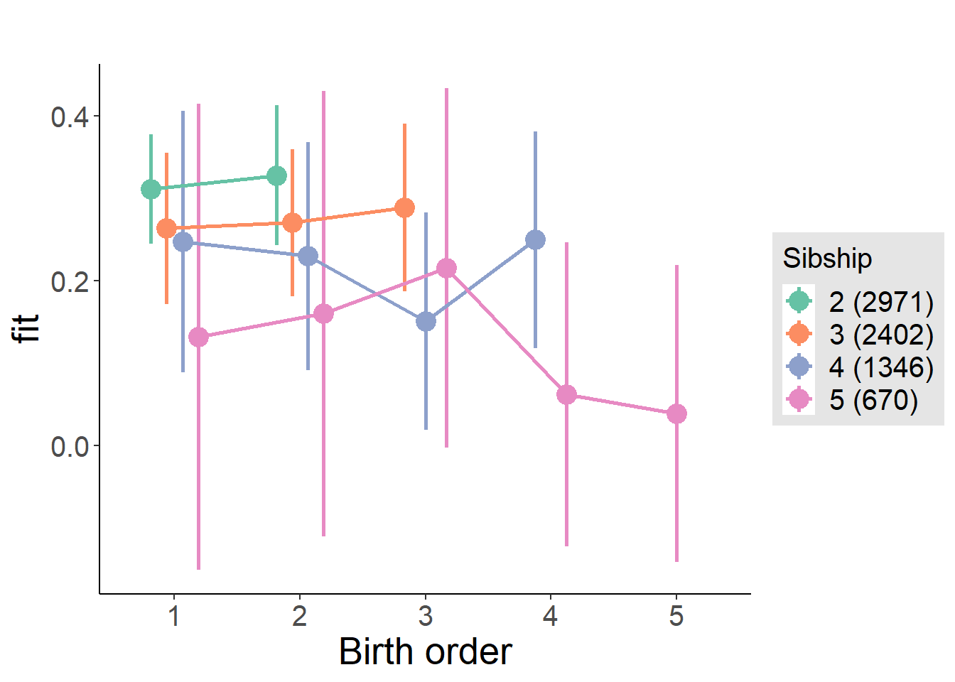
Model Comparison
###### Model 1 - Model 2
anova(m1_covariates_only, m2_birthorder_linear, m3_birthorder_nonlinear, m4_interaction)
## refitting model(s) with ML (instead of REML)| Df | AIC | BIC | logLik | deviance | Chisq | Chi Df | Pr(>Chisq) |
|---|---|---|---|---|---|---|---|
| 10 | 19207 | 19276 | -9594 | 19187 | NA | NA | NA |
| 11 | 19209 | 19285 | -9593 | 19187 | 0.07694 | 1 | 0.7815 |
| 14 | 19213 | 19310 | -9593 | 19185 | 1.686 | 3 | 0.6402 |
| 20 | 19218 | 19356 | -9589 | 19178 | 6.998 | 6 | 0.3211 |
Compare birth order specifications
library(coefplot)
multiplot(outcome_naive_m1, outcome_preg_m1, outcome_uterus_m1, outcome_parental_m1, dodgeHeight = 0.6,
          intercept = FALSE)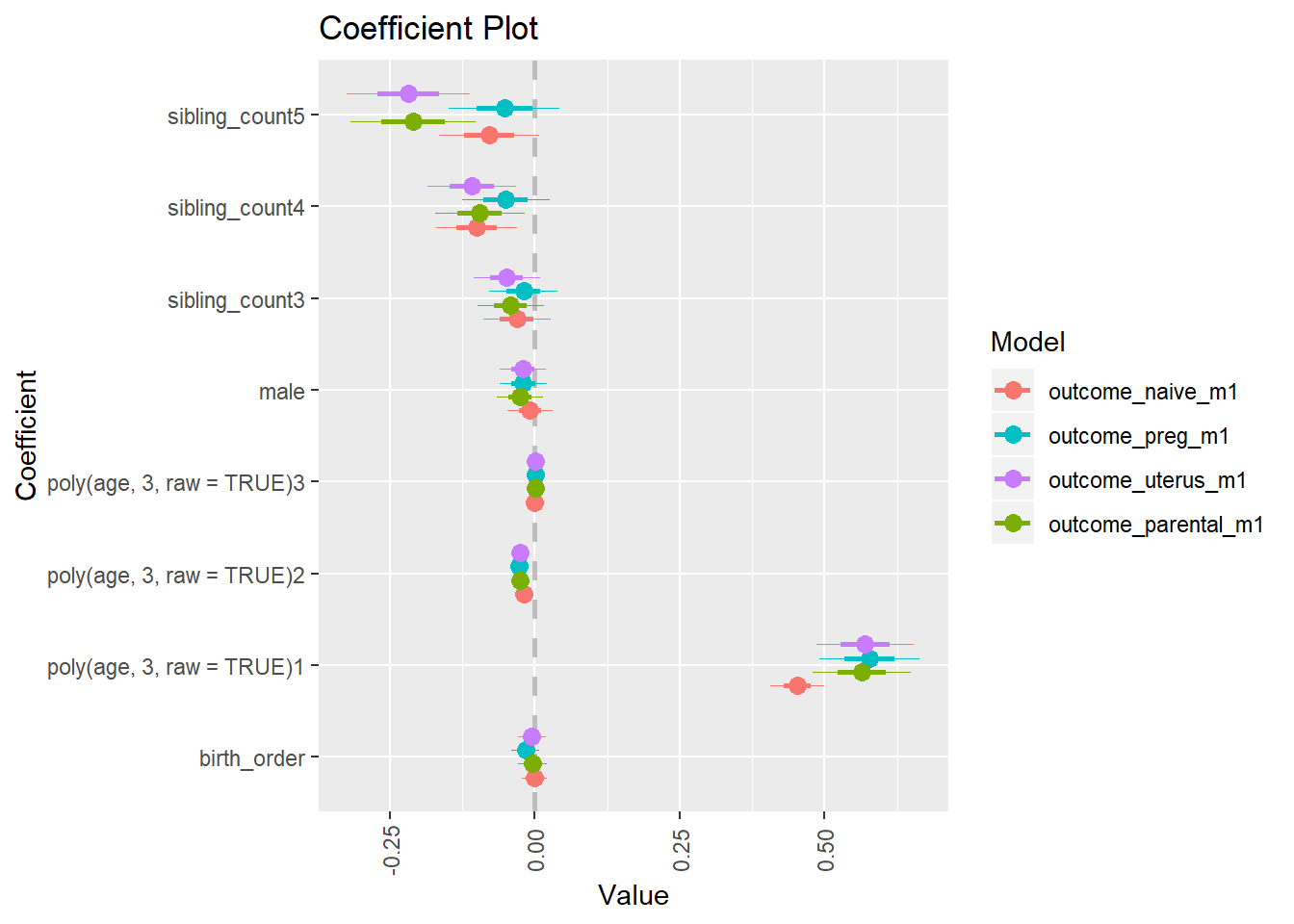
g-factor 2007 old
birthorder <- birthorder %>% mutate(outcome = g_factor_2007_old)
model = lmer(outcome ~ birth_order + poly(age, 3, raw = TRUE) + male + sibling_count + (1 | mother_pidlink),
                   data = birthorder)
compare_birthorder_specs(model)
Naive birth order
outcome_naive_m1 <- update(m2_birthorder_linear, data = birthorder %>%
                     mutate(sibling_count = sibling_count_naive_factor,
                            birth_order_nonlinear = birthorder_naive_factor,
                            birth_order = birthorder_naive,
                            count_birth_order = count_birthorder_naive) %>%
                     filter(sibling_count != "1"))
compare_models_markdown(outcome_naive_m1)
Basic Model
Model Summary
m1_covariates_only <- update(m2_birthorder_linear, formula = . ~ . - birth_order)
tidy(m1_covariates_only, conf.int = T, conf.level = 0.995)| effect | group | term | estimate | std.error | statistic | df | p.value | conf.low | conf.high |
|---|---|---|---|---|---|---|---|---|---|
| fixed | NA | (Intercept) | -3.042 | 2.574 | -1.182 | 3255 | 0.2375 | -10.27 | 4.185 |
| fixed | NA | poly(age, 3, raw = TRUE)1 | 0.3752 | 0.2695 | 1.392 | 3256 | 0.1639 | -0.3812 | 1.132 |
| fixed | NA | poly(age, 3, raw = TRUE)2 | -0.01334 | 0.009287 | -1.436 | 3258 | 0.151 | -0.03941 | 0.01273 |
| fixed | NA | poly(age, 3, raw = TRUE)3 | 0.0001442 | 0.0001053 | 1.369 | 3259 | 0.171 | -0.0001514 | 0.0004399 |
| fixed | NA | male | 0.1155 | 0.0318 | 3.632 | 3001 | 0.000286 | 0.02623 | 0.2048 |
| fixed | NA | sibling_count3 | -0.01357 | 0.0549 | -0.2471 | 2386 | 0.8048 | -0.1677 | 0.1405 |
| fixed | NA | sibling_count4 | -0.1226 | 0.05373 | -2.281 | 2289 | 0.02262 | -0.2734 | 0.02824 |
| fixed | NA | sibling_count5 | -0.02873 | 0.05463 | -0.5258 | 2145 | 0.5991 | -0.1821 | 0.1246 |
| ran_pars | mother_pidlink | sd__(Intercept) | 0.5363 | NA | NA | NA | NA | NA | NA |
| ran_pars | Residual | sd__Observation | 0.7785 | NA | NA | NA | NA | NA | NA |
Coefficient Plot
plot(allEffects(m1_covariates_only, confidence.level = 0.995))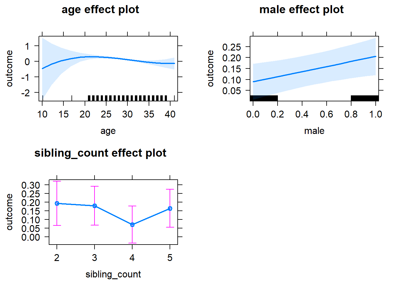
Add Birth Order Linear
Model Summary
tidy(m2_birthorder_linear, conf.int = T, conf.level = 0.995)| effect | group | term | estimate | std.error | statistic | df | p.value | conf.low | conf.high |
|---|---|---|---|---|---|---|---|---|---|
| fixed | NA | (Intercept) | -2.887 | 2.575 | -1.121 | 3254 | 0.2623 | -10.11 | 4.341 |
| fixed | NA | birth_order | -0.02725 | 0.01454 | -1.873 | 2890 | 0.06113 | -0.06807 | 0.01358 |
| fixed | NA | poly(age, 3, raw = TRUE)1 | 0.3639 | 0.2694 | 1.351 | 3255 | 0.1769 | -0.3924 | 1.12 |
| fixed | NA | poly(age, 3, raw = TRUE)2 | -0.01297 | 0.009286 | -1.397 | 3257 | 0.1627 | -0.03903 | 0.0131 |
| fixed | NA | poly(age, 3, raw = TRUE)3 | 0.0001401 | 0.0001053 | 1.33 | 3258 | 0.1837 | -0.0001556 | 0.0004357 |
| fixed | NA | male | 0.1156 | 0.03178 | 3.637 | 2998 | 0.0002808 | 0.02637 | 0.2048 |
| fixed | NA | sibling_count3 | -0.001359 | 0.05528 | -0.02458 | 2419 | 0.9804 | -0.1565 | 0.1538 |
| fixed | NA | sibling_count4 | -0.09776 | 0.05534 | -1.767 | 2425 | 0.07741 | -0.2531 | 0.05757 |
| fixed | NA | sibling_count5 | 0.01099 | 0.0586 | 0.1876 | 2449 | 0.8512 | -0.1535 | 0.1755 |
| ran_pars | mother_pidlink | sd__(Intercept) | 0.5373 | NA | NA | NA | NA | NA | NA |
| ran_pars | Residual | sd__Observation | 0.7776 | NA | NA | NA | NA | NA | NA |
Coefficient Plot
plot_birthorder2(m2_birthorder_linear, separate = FALSE)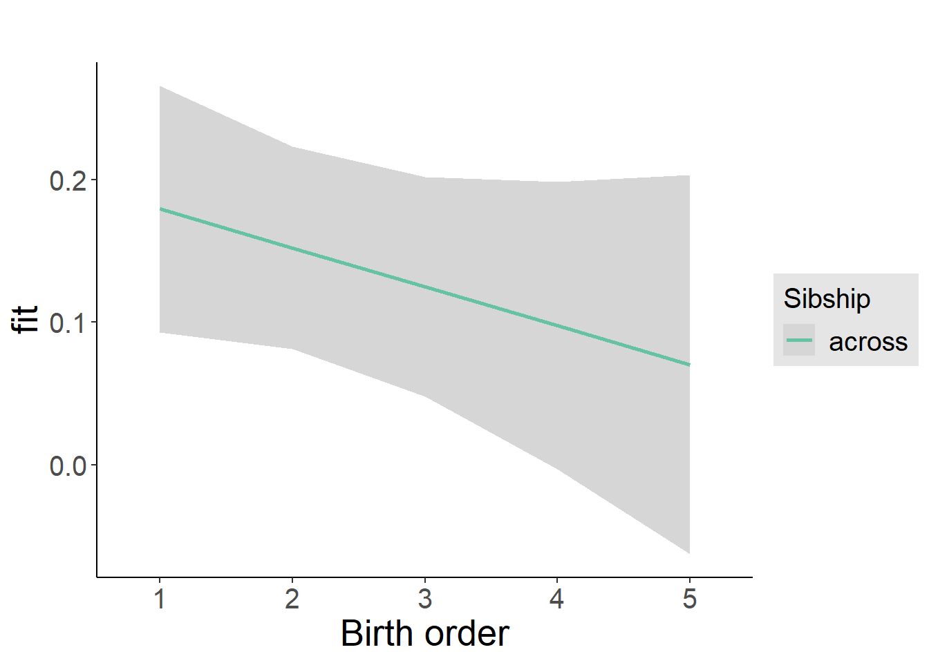
Add Birth Order Factor
Model Summary
m3_birthorder_nonlinear = update(m1_covariates_only, formula = . ~ . + birth_order_nonlinear)
tidy(m3_birthorder_nonlinear, conf.int = T, conf.level = 0.995)| effect | group | term | estimate | std.error | statistic | df | p.value | conf.low | conf.high |
|---|---|---|---|---|---|---|---|---|---|
| fixed | NA | (Intercept) | -2.677 | 2.576 | -1.039 | 3252 | 0.2987 | -9.908 | 4.554 |
| fixed | NA | poly(age, 3, raw = TRUE)1 | 0.3442 | 0.2696 | 1.277 | 3253 | 0.2018 | -0.4126 | 1.101 |
| fixed | NA | poly(age, 3, raw = TRUE)2 | -0.01239 | 0.009291 | -1.334 | 3254 | 0.1824 | -0.03847 | 0.01369 |
| fixed | NA | poly(age, 3, raw = TRUE)3 | 0.0001349 | 0.0001054 | 1.281 | 3255 | 0.2004 | -0.0001608 | 0.0004307 |
| fixed | NA | male | 0.1165 | 0.03178 | 3.665 | 2998 | 0.0002513 | 0.02727 | 0.2057 |
| fixed | NA | sibling_count3 | 0.009002 | 0.05621 | 0.1602 | 2509 | 0.8728 | -0.1488 | 0.1668 |
| fixed | NA | sibling_count4 | -0.09129 | 0.05612 | -1.627 | 2512 | 0.1039 | -0.2488 | 0.06623 |
| fixed | NA | sibling_count5 | -0.004278 | 0.05906 | -0.07243 | 2491 | 0.9423 | -0.17 | 0.1615 |
| fixed | NA | birth_order_nonlinear2 | -0.09063 | 0.03864 | -2.345 | 2486 | 0.01908 | -0.1991 | 0.01784 |
| fixed | NA | birth_order_nonlinear3 | -0.1202 | 0.0446 | -2.696 | 2472 | 0.007066 | -0.2454 | 0.004953 |
| fixed | NA | birth_order_nonlinear4 | -0.1009 | 0.0553 | -1.825 | 2637 | 0.06811 | -0.2561 | 0.0543 |
| fixed | NA | birth_order_nonlinear5 | -0.01561 | 0.07873 | -0.1983 | 2622 | 0.8428 | -0.2366 | 0.2054 |
| ran_pars | mother_pidlink | sd__(Intercept) | 0.5356 | NA | NA | NA | NA | NA | NA |
| ran_pars | Residual | sd__Observation | 0.7778 | NA | NA | NA | NA | NA | NA |
Coefficient Plot
plot_birthorder(m3_birthorder_nonlinear, separate = FALSE)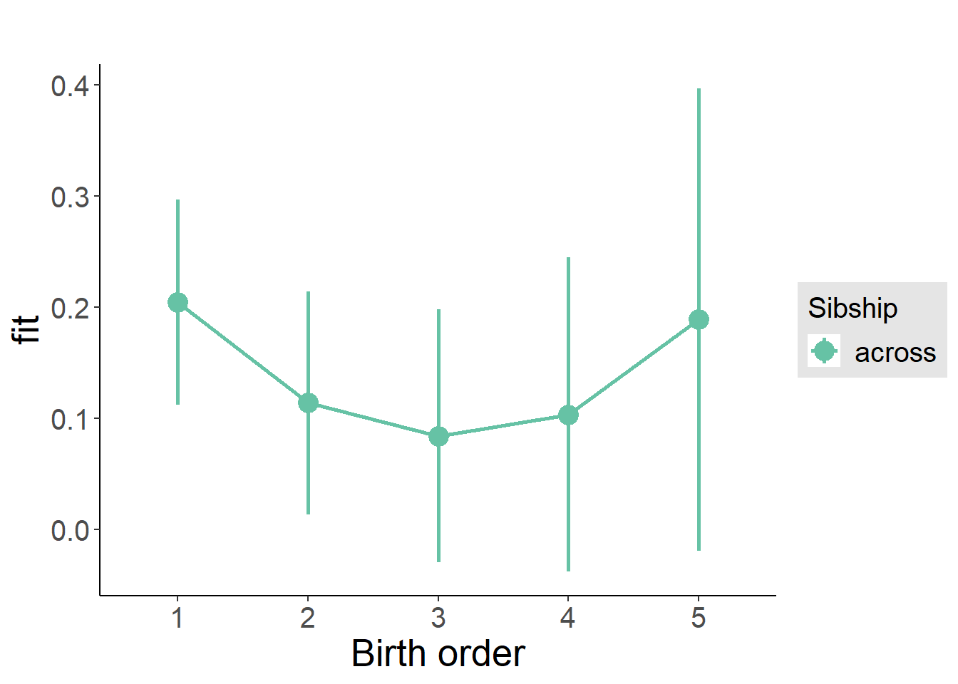
Add Interaction
Model Summary
m4_interaction = update(m3_birthorder_nonlinear, formula = . ~ . - birth_order_nonlinear - sibling_count + count_birth_order)
tidy(m4_interaction, conf.int = T, conf.level = 0.995)| effect | group | term | estimate | std.error | statistic | df | p.value | conf.low | conf.high |
|---|---|---|---|---|---|---|---|---|---|
| fixed | NA | (Intercept) | -2.973 | 2.578 | -1.153 | 3246 | 0.2489 | -10.21 | 4.263 |
| fixed | NA | poly(age, 3, raw = TRUE)1 | 0.375 | 0.2698 | 1.39 | 3247 | 0.1646 | -0.3822 | 1.132 |
| fixed | NA | poly(age, 3, raw = TRUE)2 | -0.01341 | 0.009297 | -1.442 | 3248 | 0.1494 | -0.0395 | 0.01269 |
| fixed | NA | poly(age, 3, raw = TRUE)3 | 0.0001459 | 0.0001054 | 1.384 | 3249 | 0.1664 | -0.00015 | 0.0004419 |
| fixed | NA | male | 0.1144 | 0.0318 | 3.596 | 2995 | 0.0003285 | 0.02509 | 0.2036 |
| fixed | NA | count_birth_order2/2 | -0.1172 | 0.0734 | -1.597 | 2569 | 0.1105 | -0.3232 | 0.08884 |
| fixed | NA | count_birth_order1/3 | -0.02158 | 0.074 | -0.2916 | 3227 | 0.7706 | -0.2293 | 0.1861 |
| fixed | NA | count_birth_order2/3 | -0.05197 | 0.07895 | -0.6582 | 3249 | 0.5104 | -0.2736 | 0.1696 |
| fixed | NA | count_birth_order3/3 | -0.1374 | 0.07922 | -1.734 | 3248 | 0.08293 | -0.3598 | 0.08497 |
| fixed | NA | count_birth_order1/4 | -0.07658 | 0.07624 | -1.004 | 3244 | 0.3153 | -0.2906 | 0.1374 |
| fixed | NA | count_birth_order2/4 | -0.1582 | 0.07938 | -1.993 | 3248 | 0.04634 | -0.381 | 0.06461 |
| fixed | NA | count_birth_order3/4 | -0.3096 | 0.08162 | -3.794 | 3235 | 0.0001511 | -0.5388 | -0.08054 |
| fixed | NA | count_birth_order4/4 | -0.1979 | 0.08237 | -2.402 | 3248 | 0.01635 | -0.4291 | 0.03335 |
| fixed | NA | count_birth_order1/5 | -0.03977 | 0.08352 | -0.4761 | 3244 | 0.634 | -0.2742 | 0.1947 |
| fixed | NA | count_birth_order2/5 | -0.1867 | 0.08495 | -2.198 | 3235 | 0.02805 | -0.4251 | 0.05178 |
| fixed | NA | count_birth_order3/5 | -0.02341 | 0.08385 | -0.2793 | 3224 | 0.7801 | -0.2588 | 0.2119 |
| fixed | NA | count_birth_order4/5 | -0.1285 | 0.0857 | -1.499 | 3208 | 0.1339 | -0.3691 | 0.1121 |
| fixed | NA | count_birth_order5/5 | -0.0269 | 0.0875 | -0.3075 | 3232 | 0.7585 | -0.2725 | 0.2187 |
| ran_pars | mother_pidlink | sd__(Intercept) | 0.5328 | NA | NA | NA | NA | NA | NA |
| ran_pars | Residual | sd__Observation | 0.7788 | NA | NA | NA | NA | NA | NA |
Coefficient Plot
plot_birthorder(m4_interaction)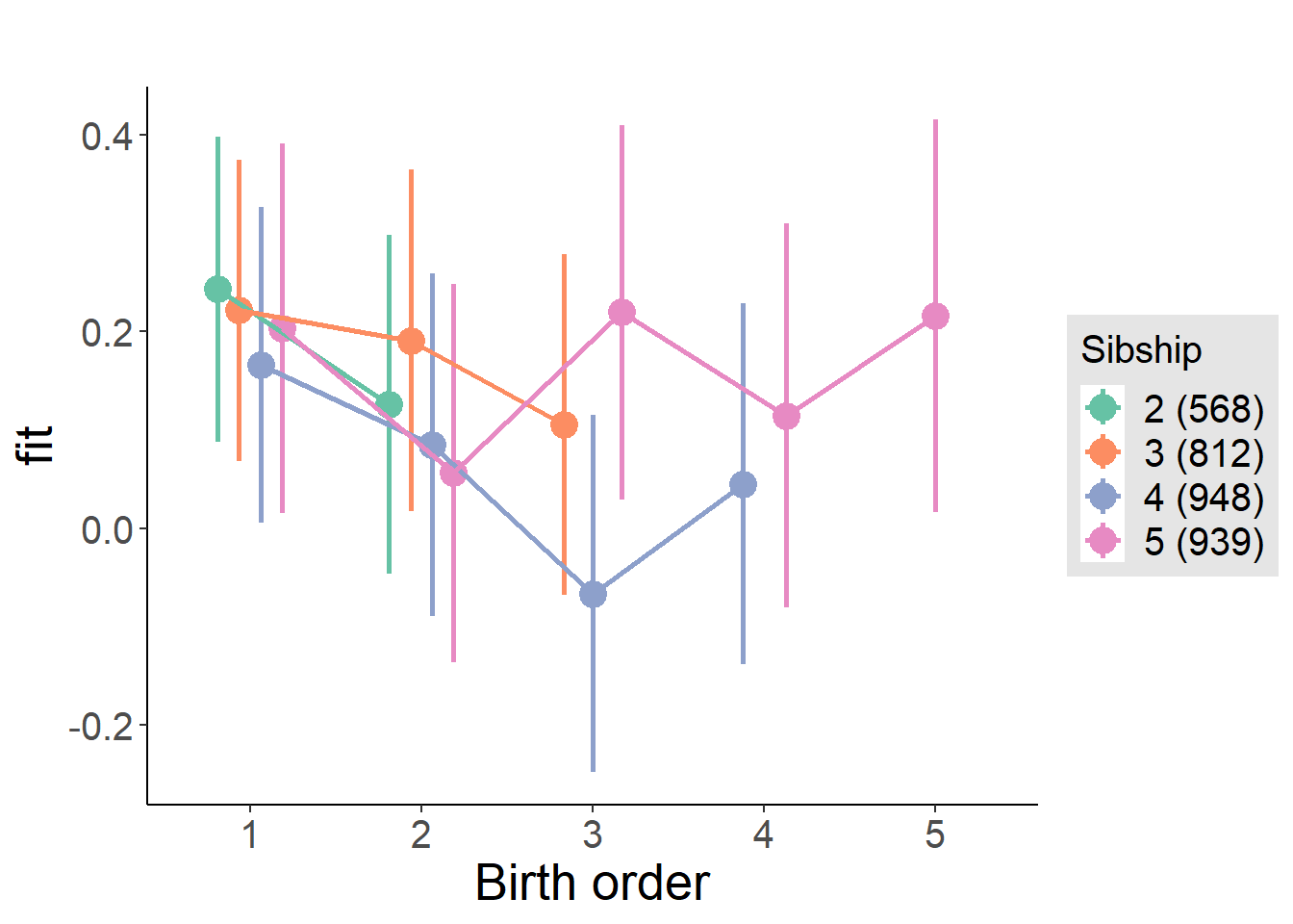
Model Comparison
###### Model 1 - Model 2
anova(m1_covariates_only, m2_birthorder_linear, m3_birthorder_nonlinear, m4_interaction)
## refitting model(s) with ML (instead of REML)| Df | AIC | BIC | logLik | deviance | Chisq | Chi Df | Pr(>Chisq) |
|---|---|---|---|---|---|---|---|
| 10 | 8787 | 8848 | -4383 | 8767 | NA | NA | NA |
| 11 | 8785 | 8852 | -4382 | 8763 | 3.511 | 1 | 0.06095 |
| 14 | 8784 | 8870 | -4378 | 8756 | 6.802 | 3 | 0.07848 |
| 20 | 8787 | 8909 | -4374 | 8747 | 8.975 | 6 | 0.175 |
Maternal birth order
outcome_uterus_m1 <- update(m2_birthorder_linear, data = birthorder %>%
                     mutate(sibling_count = sibling_count_uterus_alive_factor,
                            birth_order_nonlinear = birthorder_uterus_alive_factor,
                            birth_order = birthorder_uterus_alive,
                            count_birth_order = count_birthorder_uterus_alive) %>%
                     filter(sibling_count != "1"))
compare_models_markdown(outcome_uterus_m1)
Basic Model
Model Summary
m1_covariates_only <- update(m2_birthorder_linear, formula = . ~ . - birth_order)
tidy(m1_covariates_only, conf.int = T, conf.level = 0.995)| effect | group | term | estimate | std.error | statistic | df | p.value | conf.low | conf.high |
|---|---|---|---|---|---|---|---|---|---|
| fixed | NA | (Intercept) | -4.049 | 4.157 | -0.9739 | 2238 | 0.3302 | -15.72 | 7.621 |
| fixed | NA | poly(age, 3, raw = TRUE)1 | 0.4708 | 0.4346 | 1.083 | 2235 | 0.2788 | -0.7492 | 1.691 |
| fixed | NA | poly(age, 3, raw = TRUE)2 | -0.01623 | 0.01493 | -1.087 | 2230 | 0.277 | -0.05814 | 0.02567 |
| fixed | NA | poly(age, 3, raw = TRUE)3 | 0.0001811 | 0.0001685 | 1.074 | 2226 | 0.2828 | -0.0002921 | 0.0006542 |
| fixed | NA | male | 0.01779 | 0.03242 | 0.5488 | 2355 | 0.5832 | -0.07322 | 0.1088 |
| fixed | NA | sibling_count3 | 0.006539 | 0.05033 | 0.1299 | 1780 | 0.8967 | -0.1348 | 0.1478 |
| fixed | NA | sibling_count4 | -0.1089 | 0.05217 | -2.088 | 1700 | 0.03693 | -0.2554 | 0.0375 |
| fixed | NA | sibling_count5 | -0.1734 | 0.05708 | -3.038 | 1644 | 0.00242 | -0.3336 | -0.01317 |
| ran_pars | mother_pidlink | sd__(Intercept) | 0.4654 | NA | NA | NA | NA | NA | NA |
| ran_pars | Residual | sd__Observation | 0.7075 | NA | NA | NA | NA | NA | NA |
Coefficient Plot
plot(allEffects(m1_covariates_only, confidence.level = 0.995))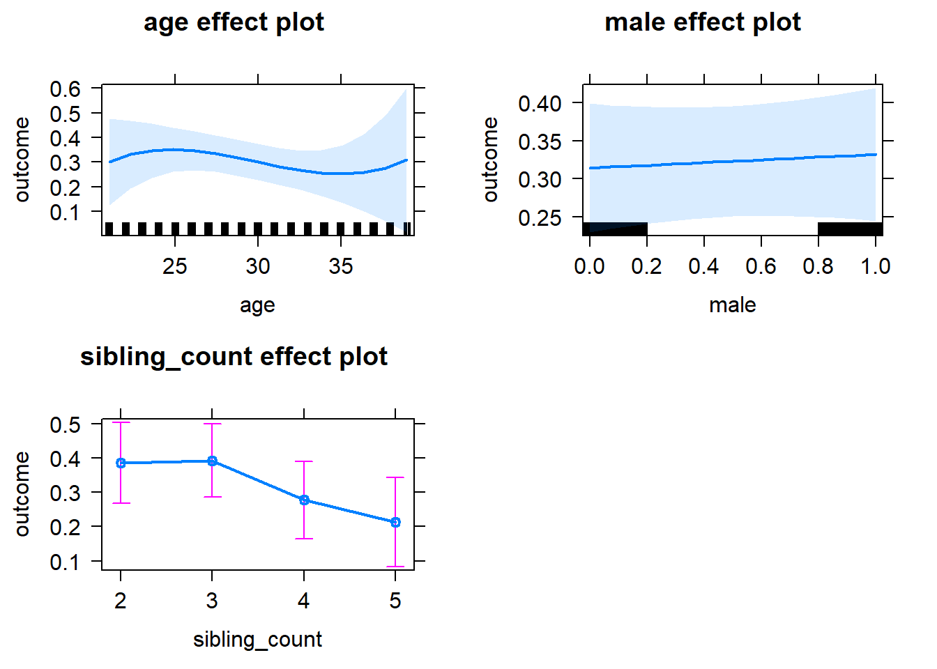
Add Birth Order Linear
Model Summary
tidy(m2_birthorder_linear, conf.int = T, conf.level = 0.995)| effect | group | term | estimate | std.error | statistic | df | p.value | conf.low | conf.high |
|---|---|---|---|---|---|---|---|---|---|
| fixed | NA | (Intercept) | -4.21 | 4.159 | -1.012 | 2239 | 0.3115 | -15.88 | 7.464 |
| fixed | NA | birth_order | 0.01819 | 0.01657 | 1.098 | 2445 | 0.2725 | -0.02833 | 0.06471 |
| fixed | NA | poly(age, 3, raw = TRUE)1 | 0.4854 | 0.4348 | 1.116 | 2234 | 0.2643 | -0.735 | 1.706 |
| fixed | NA | poly(age, 3, raw = TRUE)2 | -0.01677 | 0.01493 | -1.123 | 2230 | 0.2617 | -0.05869 | 0.02516 |
| fixed | NA | poly(age, 3, raw = TRUE)3 | 0.0001877 | 0.0001686 | 1.113 | 2225 | 0.2657 | -0.0002856 | 0.000661 |
| fixed | NA | male | 0.01756 | 0.03242 | 0.5416 | 2354 | 0.5882 | -0.07344 | 0.1086 |
| fixed | NA | sibling_count3 | -0.001135 | 0.05083 | -0.02234 | 1800 | 0.9822 | -0.1438 | 0.1415 |
| fixed | NA | sibling_count4 | -0.1285 | 0.05514 | -2.33 | 1770 | 0.0199 | -0.2833 | 0.02628 |
| fixed | NA | sibling_count5 | -0.2059 | 0.06431 | -3.202 | 1859 | 0.001389 | -0.3864 | -0.02539 |
| ran_pars | mother_pidlink | sd__(Intercept) | 0.4662 | NA | NA | NA | NA | NA | NA |
| ran_pars | Residual | sd__Observation | 0.707 | NA | NA | NA | NA | NA | NA |
Coefficient Plot
plot_birthorder2(m2_birthorder_linear, separate = FALSE)
Add Birth Order Factor
Model Summary
m3_birthorder_nonlinear = update(m1_covariates_only, formula = . ~ . + birth_order_nonlinear)
tidy(m3_birthorder_nonlinear, conf.int = T, conf.level = 0.995)| effect | group | term | estimate | std.error | statistic | df | p.value | conf.low | conf.high |
|---|---|---|---|---|---|---|---|---|---|
| fixed | NA | (Intercept) | -4.218 | 4.163 | -1.013 | 2236 | 0.311 | -15.9 | 7.467 |
| fixed | NA | poly(age, 3, raw = TRUE)1 | 0.4896 | 0.4352 | 1.125 | 2231 | 0.2608 | -0.7321 | 1.711 |
| fixed | NA | poly(age, 3, raw = TRUE)2 | -0.01692 | 0.01495 | -1.132 | 2226 | 0.2578 | -0.05889 | 0.02504 |
| fixed | NA | poly(age, 3, raw = TRUE)3 | 0.0001896 | 0.0001688 | 1.124 | 2221 | 0.2613 | -0.0002842 | 0.0006634 |
| fixed | NA | male | 0.01723 | 0.03244 | 0.5311 | 2350 | 0.5954 | -0.07383 | 0.1083 |
| fixed | NA | sibling_count3 | -0.003582 | 0.05136 | -0.06974 | 1849 | 0.9444 | -0.1478 | 0.1406 |
| fixed | NA | sibling_count4 | -0.1342 | 0.05588 | -2.401 | 1823 | 0.01645 | -0.291 | 0.02269 |
| fixed | NA | sibling_count5 | -0.2109 | 0.06508 | -3.241 | 1895 | 0.001212 | -0.3936 | -0.02824 |
| fixed | NA | birth_order_nonlinear2 | -0.009857 | 0.03808 | -0.2589 | 1861 | 0.7958 | -0.1168 | 0.09704 |
| fixed | NA | birth_order_nonlinear3 | 0.04096 | 0.0471 | 0.8695 | 2055 | 0.3847 | -0.09127 | 0.1732 |
| fixed | NA | birth_order_nonlinear4 | 0.06328 | 0.06293 | 1.006 | 2292 | 0.3147 | -0.1134 | 0.2399 |
| fixed | NA | birth_order_nonlinear5 | 0.05697 | 0.09433 | 0.6039 | 2201 | 0.546 | -0.2078 | 0.3218 |
| ran_pars | mother_pidlink | sd__(Intercept) | 0.4665 | NA | NA | NA | NA | NA | NA |
| ran_pars | Residual | sd__Observation | 0.7073 | NA | NA | NA | NA | NA | NA |
Coefficient Plot
plot_birthorder(m3_birthorder_nonlinear, separate = FALSE)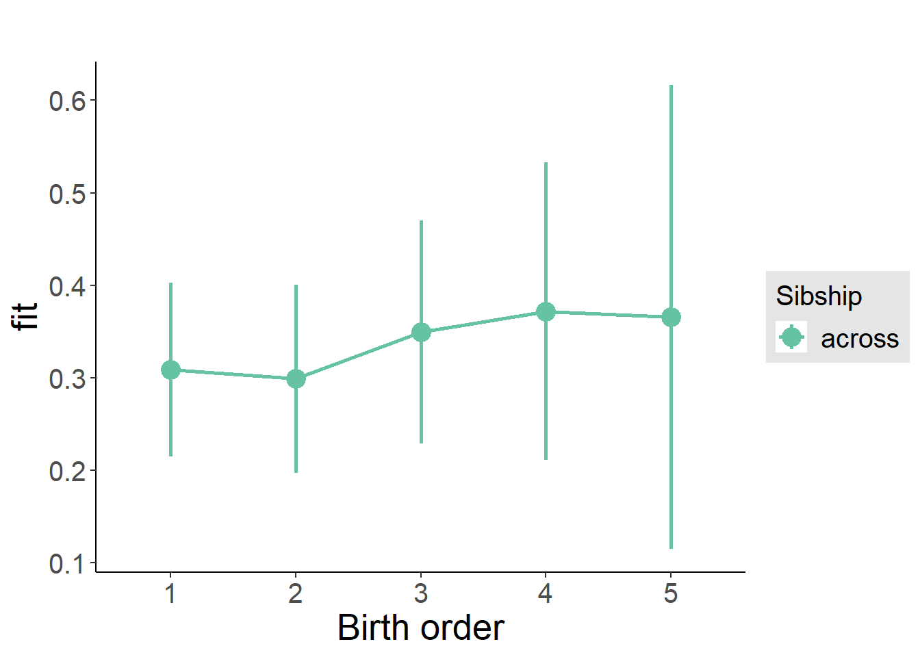
Add Interaction
Model Summary
m4_interaction = update(m3_birthorder_nonlinear, formula = . ~ . - birth_order_nonlinear - sibling_count + count_birth_order)
tidy(m4_interaction, conf.int = T, conf.level = 0.995)| effect | group | term | estimate | std.error | statistic | df | p.value | conf.low | conf.high |
|---|---|---|---|---|---|---|---|---|---|
| fixed | NA | (Intercept) | -4.419 | 4.161 | -1.062 | 2226 | 0.2883 | -16.1 | 7.26 |
| fixed | NA | poly(age, 3, raw = TRUE)1 | 0.5147 | 0.435 | 1.183 | 2221 | 0.2368 | -0.7063 | 1.736 |
| fixed | NA | poly(age, 3, raw = TRUE)2 | -0.01783 | 0.01494 | -1.193 | 2216 | 0.2328 | -0.05977 | 0.02411 |
| fixed | NA | poly(age, 3, raw = TRUE)3 | 0.0002004 | 0.0001687 | 1.188 | 2212 | 0.235 | -0.0002731 | 0.000674 |
| fixed | NA | male | 0.01741 | 0.03247 | 0.536 | 2346 | 0.592 | -0.07375 | 0.1086 |
| fixed | NA | count_birth_order2/2 | -0.08644 | 0.06784 | -1.274 | 1862 | 0.2028 | -0.2769 | 0.104 |
| fixed | NA | count_birth_order1/3 | -0.05432 | 0.06349 | -0.8555 | 2492 | 0.3923 | -0.2325 | 0.1239 |
| fixed | NA | count_birth_order2/3 | 0.01796 | 0.06945 | 0.2586 | 2526 | 0.796 | -0.177 | 0.2129 |
| fixed | NA | count_birth_order3/3 | -0.02227 | 0.07689 | -0.2897 | 2524 | 0.7721 | -0.2381 | 0.1936 |
| fixed | NA | count_birth_order1/4 | -0.16 | 0.07415 | -2.157 | 2520 | 0.03109 | -0.3681 | 0.04819 |
| fixed | NA | count_birth_order2/4 | -0.1696 | 0.07555 | -2.245 | 2526 | 0.02486 | -0.3817 | 0.04246 |
| fixed | NA | count_birth_order3/4 | -0.1822 | 0.07645 | -2.383 | 2515 | 0.01724 | -0.3968 | 0.03241 |
| fixed | NA | count_birth_order4/4 | -0.02882 | 0.08303 | -0.3471 | 2519 | 0.7285 | -0.2619 | 0.2042 |
| fixed | NA | count_birth_order1/5 | -0.2606 | 0.09569 | -2.723 | 2523 | 0.006511 | -0.5292 | 0.008027 |
| fixed | NA | count_birth_order2/5 | -0.3084 | 0.09884 | -3.12 | 2490 | 0.001829 | -0.5859 | -0.03095 |
| fixed | NA | count_birth_order3/5 | -0.04529 | 0.08998 | -0.5034 | 2488 | 0.6147 | -0.2979 | 0.2073 |
| fixed | NA | count_birth_order4/5 | -0.2563 | 0.08942 | -2.867 | 2500 | 0.004184 | -0.5073 | -0.005324 |
| fixed | NA | count_birth_order5/5 | -0.1791 | 0.09358 | -1.913 | 2501 | 0.0558 | -0.4418 | 0.08362 |
| ran_pars | mother_pidlink | sd__(Intercept) | 0.4688 | NA | NA | NA | NA | NA | NA |
| ran_pars | Residual | sd__Observation | 0.705 | NA | NA | NA | NA | NA | NA |
Coefficient Plot
plot_birthorder(m4_interaction)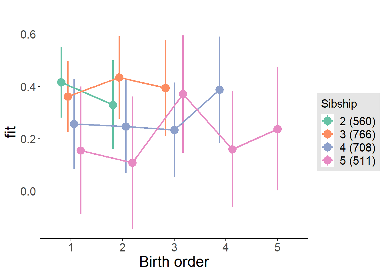
Model Comparison
###### Model 1 - Model 2
anova(m1_covariates_only, m2_birthorder_linear, m3_birthorder_nonlinear, m4_interaction)
## refitting model(s) with ML (instead of REML)| Df | AIC | BIC | logLik | deviance | Chisq | Chi Df | Pr(>Chisq) |
|---|---|---|---|---|---|---|---|
| 10 | 6301 | 6359 | -3140 | 6281 | NA | NA | NA |
| 11 | 6302 | 6366 | -3140 | 6280 | 1.205 | 1 | 0.2722 |
| 14 | 6307 | 6388 | -3139 | 6279 | 0.817 | 3 | 0.8454 |
| 20 | 6307 | 6424 | -3133 | 6267 | 11.91 | 6 | 0.06407 |
Maternal pregnancy order
outcome_preg_m1 <- update(m2_birthorder_linear, data = birthorder %>%
  mutate(sibling_count = sibling_count_uterus_preg_factor,
         birth_order_nonlinear = birthorder_uterus_preg_factor,
         birth_order = birthorder_uterus_preg,
         count_birth_order = count_birthorder_uterus_preg
         ) %>%
    filter(sibling_count != "1"))
compare_models_markdown(outcome_preg_m1)
Basic Model
Model Summary
m1_covariates_only <- update(m2_birthorder_linear, formula = . ~ . - birth_order)
tidy(m1_covariates_only, conf.int = T, conf.level = 0.995)| effect | group | term | estimate | std.error | statistic | df | p.value | conf.low | conf.high |
|---|---|---|---|---|---|---|---|---|---|
| fixed | NA | (Intercept) | -1.864 | 4.382 | -0.4254 | 2052 | 0.6706 | -14.16 | 10.44 |
| fixed | NA | poly(age, 3, raw = TRUE)1 | 0.2282 | 0.4587 | 0.4975 | 2049 | 0.6189 | -1.059 | 1.516 |
| fixed | NA | poly(age, 3, raw = TRUE)2 | -0.007366 | 0.01577 | -0.467 | 2046 | 0.6406 | -0.05164 | 0.03691 |
| fixed | NA | poly(age, 3, raw = TRUE)3 | 0.00007476 | 0.0001783 | 0.4193 | 2042 | 0.675 | -0.0004256 | 0.0005752 |
| fixed | NA | male | 0.02406 | 0.03385 | 0.7108 | 2135 | 0.4773 | -0.07095 | 0.1191 |
| fixed | NA | sibling_count3 | -0.03132 | 0.05529 | -0.5664 | 1666 | 0.5712 | -0.1865 | 0.1239 |
| fixed | NA | sibling_count4 | -0.07875 | 0.05618 | -1.402 | 1607 | 0.1612 | -0.2365 | 0.07895 |
| fixed | NA | sibling_count5 | -0.1307 | 0.0586 | -2.231 | 1564 | 0.02585 | -0.2952 | 0.03378 |
| ran_pars | mother_pidlink | sd__(Intercept) | 0.459 | NA | NA | NA | NA | NA | NA |
| ran_pars | Residual | sd__Observation | 0.7071 | NA | NA | NA | NA | NA | NA |
Coefficient Plot
plot(allEffects(m1_covariates_only, confidence.level = 0.995))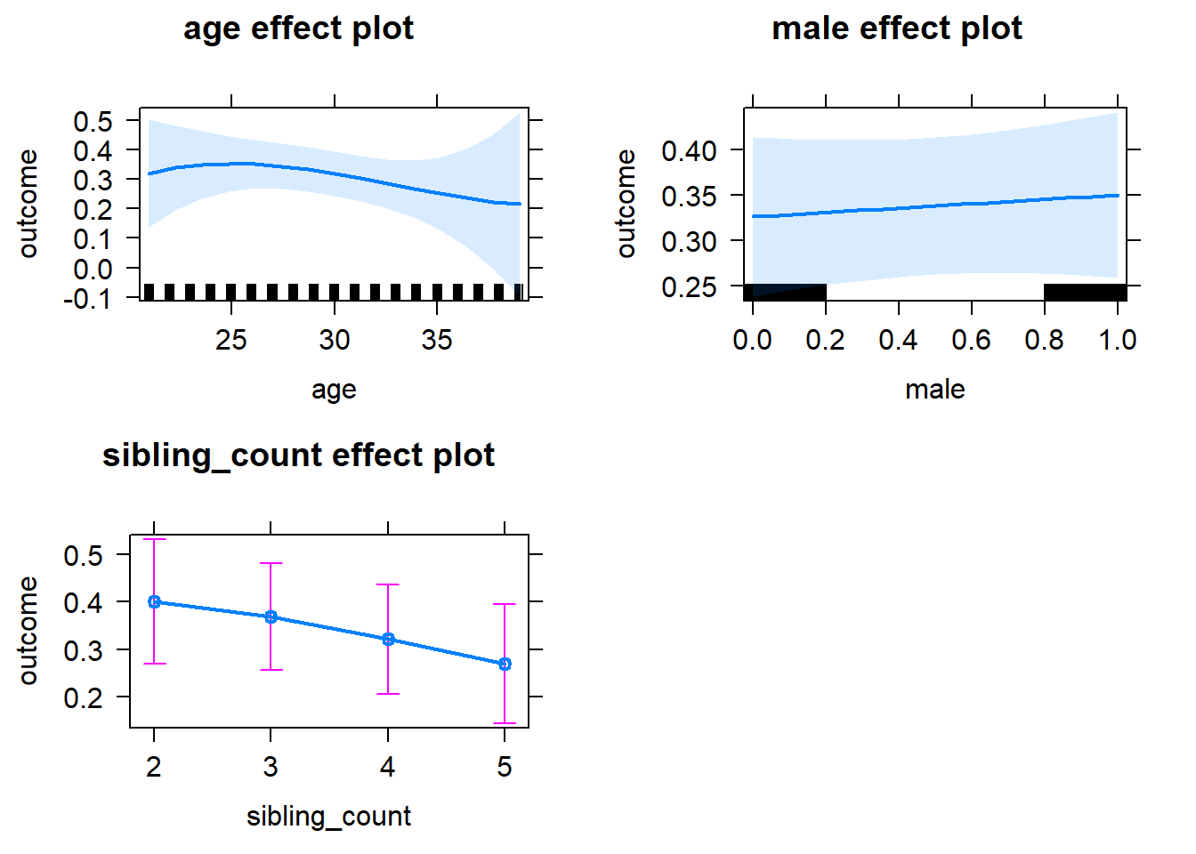
Add Birth Order Linear
Model Summary
tidy(m2_birthorder_linear, conf.int = T, conf.level = 0.995)| effect | group | term | estimate | std.error | statistic | df | p.value | conf.low | conf.high |
|---|---|---|---|---|---|---|---|---|---|
| fixed | NA | (Intercept) | -1.865 | 4.386 | -0.4251 | 2051 | 0.6708 | -14.18 | 10.45 |
| fixed | NA | birth_order | 0.00004857 | 0.01671 | 0.002906 | 2242 | 0.9977 | -0.04687 | 0.04697 |
| fixed | NA | poly(age, 3, raw = TRUE)1 | 0.2282 | 0.459 | 0.4972 | 2047 | 0.6191 | -1.06 | 1.517 |
| fixed | NA | poly(age, 3, raw = TRUE)2 | -0.007368 | 0.01579 | -0.4667 | 2044 | 0.6408 | -0.05168 | 0.03694 |
| fixed | NA | poly(age, 3, raw = TRUE)3 | 0.00007478 | 0.0001784 | 0.4191 | 2040 | 0.6752 | -0.0004261 | 0.0005757 |
| fixed | NA | male | 0.02406 | 0.03385 | 0.7106 | 2134 | 0.4774 | -0.07097 | 0.1191 |
| fixed | NA | sibling_count3 | -0.03134 | 0.05579 | -0.5617 | 1679 | 0.5744 | -0.1879 | 0.1253 |
| fixed | NA | sibling_count4 | -0.0788 | 0.05857 | -1.345 | 1652 | 0.1787 | -0.2432 | 0.08562 |
| fixed | NA | sibling_count5 | -0.1308 | 0.06441 | -2.031 | 1713 | 0.04246 | -0.3116 | 0.05002 |
| ran_pars | mother_pidlink | sd__(Intercept) | 0.4591 | NA | NA | NA | NA | NA | NA |
| ran_pars | Residual | sd__Observation | 0.7073 | NA | NA | NA | NA | NA | NA |
Coefficient Plot
plot_birthorder2(m2_birthorder_linear, separate = FALSE)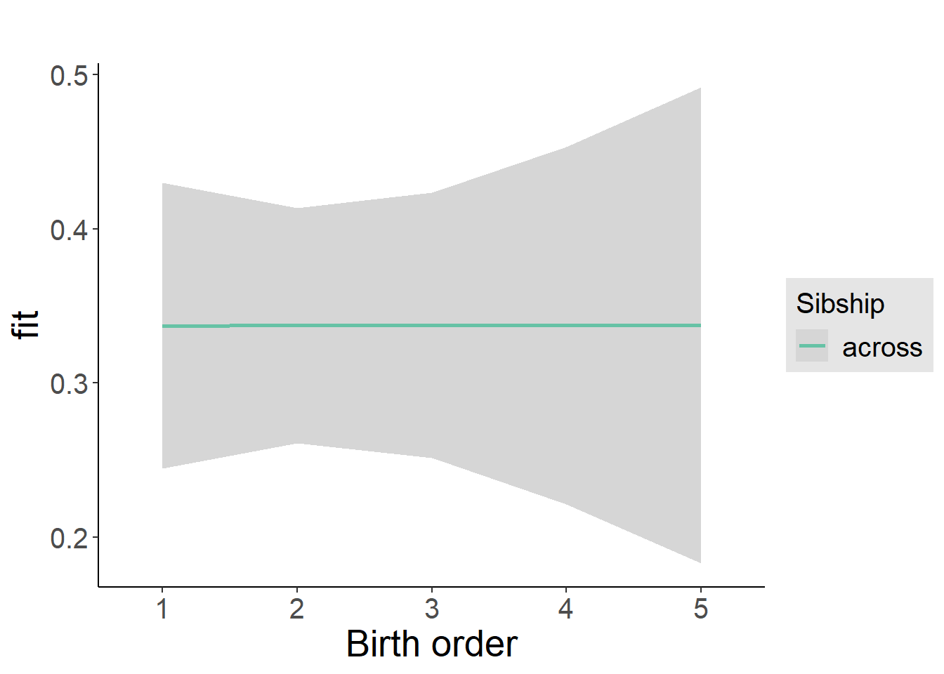
Add Birth Order Factor
Model Summary
m3_birthorder_nonlinear = update(m1_covariates_only, formula = . ~ . + birth_order_nonlinear)
tidy(m3_birthorder_nonlinear, conf.int = T, conf.level = 0.995)| effect | group | term | estimate | std.error | statistic | df | p.value | conf.low | conf.high |
|---|---|---|---|---|---|---|---|---|---|
| fixed | NA | (Intercept) | -1.762 | 4.39 | -0.4014 | 2050 | 0.6882 | -14.09 | 10.56 |
| fixed | NA | poly(age, 3, raw = TRUE)1 | 0.2178 | 0.4595 | 0.474 | 2046 | 0.6355 | -1.072 | 1.508 |
| fixed | NA | poly(age, 3, raw = TRUE)2 | -0.007016 | 0.0158 | -0.4439 | 2043 | 0.6571 | -0.05138 | 0.03734 |
| fixed | NA | poly(age, 3, raw = TRUE)3 | 0.00007091 | 0.0001786 | 0.397 | 2038 | 0.6914 | -0.0004305 | 0.0005723 |
| fixed | NA | male | 0.02363 | 0.03388 | 0.6975 | 2133 | 0.4855 | -0.07148 | 0.1187 |
| fixed | NA | sibling_count3 | -0.02587 | 0.05638 | -0.4589 | 1724 | 0.6463 | -0.1841 | 0.1324 |
| fixed | NA | sibling_count4 | -0.0723 | 0.0592 | -1.221 | 1695 | 0.2221 | -0.2385 | 0.09387 |
| fixed | NA | sibling_count5 | -0.1346 | 0.06485 | -2.076 | 1734 | 0.03804 | -0.3167 | 0.04741 |
| fixed | NA | birth_order_nonlinear2 | -0.005863 | 0.04001 | -0.1465 | 1752 | 0.8835 | -0.1182 | 0.1064 |
| fixed | NA | birth_order_nonlinear3 | -0.02504 | 0.04885 | -0.5126 | 1911 | 0.6083 | -0.1622 | 0.1121 |
| fixed | NA | birth_order_nonlinear4 | -0.008092 | 0.06495 | -0.1246 | 2070 | 0.9009 | -0.1904 | 0.1742 |
| fixed | NA | birth_order_nonlinear5 | 0.05145 | 0.09334 | 0.5512 | 2039 | 0.5816 | -0.2106 | 0.3135 |
| ran_pars | mother_pidlink | sd__(Intercept) | 0.4581 | NA | NA | NA | NA | NA | NA |
| ran_pars | Residual | sd__Observation | 0.7083 | NA | NA | NA | NA | NA | NA |
Coefficient Plot
plot_birthorder(m3_birthorder_nonlinear, separate = FALSE)
Add Interaction
Model Summary
m4_interaction = update(m3_birthorder_nonlinear, formula = . ~ . - birth_order_nonlinear - sibling_count + count_birth_order)
tidy(m4_interaction, conf.int = T, conf.level = 0.995)| effect | group | term | estimate | std.error | statistic | df | p.value | conf.low | conf.high |
|---|---|---|---|---|---|---|---|---|---|
| fixed | NA | (Intercept) | -2.114 | 4.402 | -0.4803 | 2044 | 0.6311 | -14.47 | 10.24 |
| fixed | NA | poly(age, 3, raw = TRUE)1 | 0.2561 | 0.4606 | 0.556 | 2040 | 0.5783 | -1.037 | 1.549 |
| fixed | NA | poly(age, 3, raw = TRUE)2 | -0.008386 | 0.01584 | -0.5294 | 2036 | 0.5966 | -0.05285 | 0.03608 |
| fixed | NA | poly(age, 3, raw = TRUE)3 | 0.000087 | 0.000179 | 0.486 | 2032 | 0.627 | -0.0004155 | 0.0005895 |
| fixed | NA | male | 0.02347 | 0.03395 | 0.6913 | 2128 | 0.4894 | -0.07183 | 0.1188 |
| fixed | NA | count_birth_order2/2 | -0.005311 | 0.07669 | -0.06925 | 1724 | 0.9448 | -0.2206 | 0.21 |
| fixed | NA | count_birth_order1/3 | -0.06219 | 0.07036 | -0.8838 | 2273 | 0.3769 | -0.2597 | 0.1353 |
| fixed | NA | count_birth_order2/3 | 0.01898 | 0.0764 | 0.2485 | 2298 | 0.8038 | -0.1955 | 0.2334 |
| fixed | NA | count_birth_order3/3 | -0.0448 | 0.08294 | -0.5401 | 2297 | 0.5892 | -0.2776 | 0.188 |
| fixed | NA | count_birth_order1/4 | -0.03733 | 0.0782 | -0.4774 | 2289 | 0.6331 | -0.2568 | 0.1822 |
| fixed | NA | count_birth_order2/4 | -0.1113 | 0.07891 | -1.41 | 2298 | 0.1586 | -0.3328 | 0.1102 |
| fixed | NA | count_birth_order3/4 | -0.1624 | 0.08312 | -1.953 | 2284 | 0.05089 | -0.3957 | 0.07095 |
| fixed | NA | count_birth_order4/4 | -0.006416 | 0.09156 | -0.07008 | 2286 | 0.9441 | -0.2634 | 0.2506 |
| fixed | NA | count_birth_order1/5 | -0.1064 | 0.08996 | -1.183 | 2298 | 0.2371 | -0.3589 | 0.1461 |
| fixed | NA | count_birth_order2/5 | -0.1828 | 0.09325 | -1.961 | 2287 | 0.05004 | -0.4446 | 0.07893 |
| fixed | NA | count_birth_order3/5 | -0.07218 | 0.0928 | -0.7778 | 2263 | 0.4368 | -0.3327 | 0.1883 |
| fixed | NA | count_birth_order4/5 | -0.2232 | 0.09322 | -2.395 | 2263 | 0.01672 | -0.4849 | 0.03844 |
| fixed | NA | count_birth_order5/5 | -0.08344 | 0.09662 | -0.8637 | 2275 | 0.3879 | -0.3546 | 0.1878 |
| ran_pars | mother_pidlink | sd__(Intercept) | 0.4591 | NA | NA | NA | NA | NA | NA |
| ran_pars | Residual | sd__Observation | 0.7074 | NA | NA | NA | NA | NA | NA |
Coefficient Plot
plot_birthorder(m4_interaction)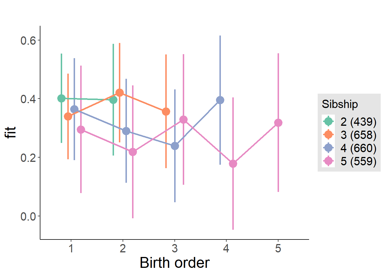
Model Comparison
###### Model 1 - Model 2
anova(m1_covariates_only, m2_birthorder_linear, m3_birthorder_nonlinear, m4_interaction)
## refitting model(s) with ML (instead of REML)| Df | AIC | BIC | logLik | deviance | Chisq | Chi Df | Pr(>Chisq) |
|---|---|---|---|---|---|---|---|
| 10 | 5719 | 5776 | -2849 | 5699 | NA | NA | NA |
| 11 | 5721 | 5784 | -2849 | 5699 | 0.000007659 | 1 | 0.9978 |
| 14 | 5726 | 5806 | -2849 | 5698 | 0.7646 | 3 | 0.8579 |
| 20 | 5730 | 5845 | -2845 | 5690 | 7.578 | 6 | 0.2707 |
Parental full sibling order
outcome_parental_m1 <- update(m2_birthorder_linear, data = birthorder %>%
  mutate(sibling_count = sibling_count_genes_factor,
         birth_order_nonlinear = birthorder_genes_factor,
         birth_order = birthorder_genes,
         count_birth_order = count_birthorder_genes
         ) %>%
      filter(sibling_count != "1"))
compare_models_markdown(outcome_parental_m1)
Basic Model
Model Summary
m1_covariates_only <- update(m2_birthorder_linear, formula = . ~ . - birth_order)
tidy(m1_covariates_only, conf.int = T, conf.level = 0.995)| effect | group | term | estimate | std.error | statistic | df | p.value | conf.low | conf.high |
|---|---|---|---|---|---|---|---|---|---|
| fixed | NA | (Intercept) | -6.229 | 4.172 | -1.493 | 2253 | 0.1355 | -17.94 | 5.481 |
| fixed | NA | poly(age, 3, raw = TRUE)1 | 0.6964 | 0.4359 | 1.598 | 2250 | 0.1103 | -0.5272 | 1.92 |
| fixed | NA | poly(age, 3, raw = TRUE)2 | -0.02388 | 0.01496 | -1.596 | 2247 | 0.1107 | -0.06588 | 0.01813 |
| fixed | NA | poly(age, 3, raw = TRUE)3 | 0.0002652 | 0.0001688 | 1.571 | 2243 | 0.1164 | -0.0002088 | 0.0007391 |
| fixed | NA | male | 0.01166 | 0.03243 | 0.3595 | 2366 | 0.7192 | -0.07938 | 0.1027 |
| fixed | NA | sibling_count3 | 0.0124 | 0.04975 | 0.2493 | 1791 | 0.8031 | -0.1272 | 0.152 |
| fixed | NA | sibling_count4 | -0.07298 | 0.05175 | -1.41 | 1720 | 0.1586 | -0.2182 | 0.07227 |
| fixed | NA | sibling_count5 | -0.1414 | 0.05802 | -2.436 | 1622 | 0.01495 | -0.3042 | 0.02152 |
| ran_pars | mother_pidlink | sd__(Intercept) | 0.4702 | NA | NA | NA | NA | NA | NA |
| ran_pars | Residual | sd__Observation | 0.7075 | NA | NA | NA | NA | NA | NA |
Coefficient Plot
plot(allEffects(m1_covariates_only, confidence.level = 0.995))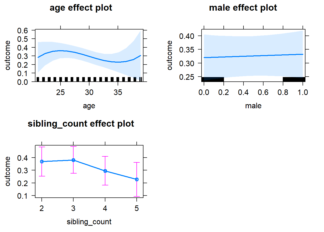
Add Birth Order Linear
Model Summary
tidy(m2_birthorder_linear, conf.int = T, conf.level = 0.995)| effect | group | term | estimate | std.error | statistic | df | p.value | conf.low | conf.high |
|---|---|---|---|---|---|---|---|---|---|
| fixed | NA | (Intercept) | -6.391 | 4.173 | -1.532 | 2254 | 0.1258 | -18.1 | 5.323 |
| fixed | NA | birth_order | 0.02125 | 0.01668 | 1.274 | 2440 | 0.2029 | -0.02558 | 0.06807 |
| fixed | NA | poly(age, 3, raw = TRUE)1 | 0.7102 | 0.436 | 1.629 | 2250 | 0.1034 | -0.5135 | 1.934 |
| fixed | NA | poly(age, 3, raw = TRUE)2 | -0.02438 | 0.01497 | -1.629 | 2247 | 0.1034 | -0.06639 | 0.01763 |
| fixed | NA | poly(age, 3, raw = TRUE)3 | 0.0002715 | 0.0001689 | 1.608 | 2243 | 0.108 | -0.0002025 | 0.0007456 |
| fixed | NA | male | 0.01127 | 0.03243 | 0.3475 | 2365 | 0.7282 | -0.07976 | 0.1023 |
| fixed | NA | sibling_count3 | 0.003248 | 0.05026 | 0.06462 | 1809 | 0.9485 | -0.1378 | 0.1443 |
| fixed | NA | sibling_count4 | -0.09601 | 0.05482 | -1.752 | 1796 | 0.08002 | -0.2499 | 0.05786 |
| fixed | NA | sibling_count5 | -0.1777 | 0.06465 | -2.748 | 1823 | 0.006051 | -0.3592 | 0.003803 |
| ran_pars | mother_pidlink | sd__(Intercept) | 0.4705 | NA | NA | NA | NA | NA | NA |
| ran_pars | Residual | sd__Observation | 0.7072 | NA | NA | NA | NA | NA | NA |
Coefficient Plot
plot_birthorder2(m2_birthorder_linear, separate = FALSE)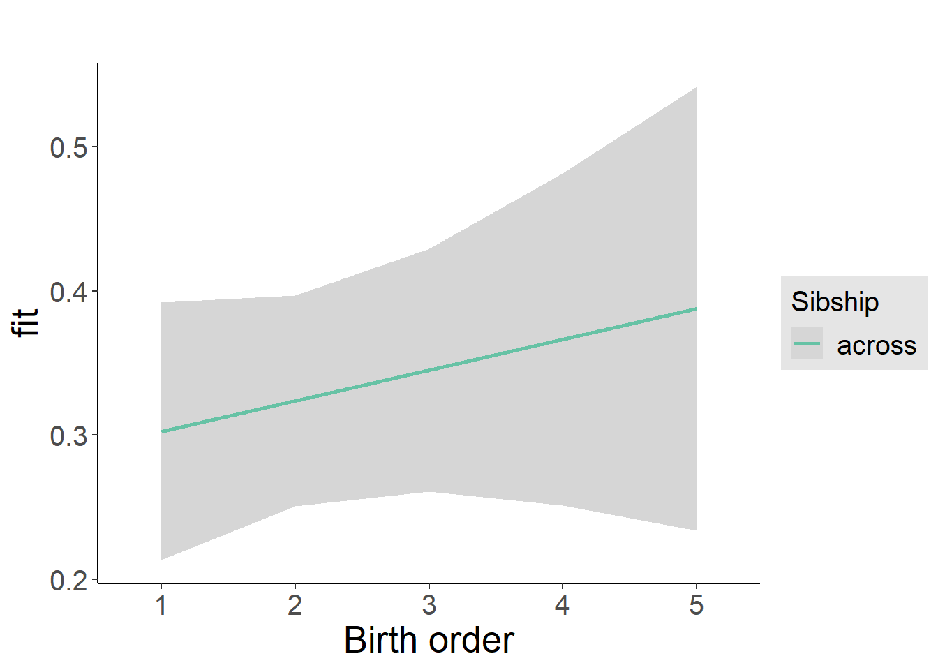
Add Birth Order Factor
Model Summary
m3_birthorder_nonlinear = update(m1_covariates_only, formula = . ~ . + birth_order_nonlinear)
tidy(m3_birthorder_nonlinear, conf.int = T, conf.level = 0.995)| effect | group | term | estimate | std.error | statistic | df | p.value | conf.low | conf.high |
|---|---|---|---|---|---|---|---|---|---|
| fixed | NA | (Intercept) | -6.414 | 4.176 | -1.536 | 2248 | 0.1247 | -18.14 | 5.308 |
| fixed | NA | poly(age, 3, raw = TRUE)1 | 0.717 | 0.4363 | 1.643 | 2244 | 0.1005 | -0.5078 | 1.942 |
| fixed | NA | poly(age, 3, raw = TRUE)2 | -0.02464 | 0.01498 | -1.645 | 2241 | 0.1001 | -0.06669 | 0.01741 |
| fixed | NA | poly(age, 3, raw = TRUE)3 | 0.0002748 | 0.000169 | 1.626 | 2237 | 0.1042 | -0.0001997 | 0.0007492 |
| fixed | NA | male | 0.01085 | 0.03245 | 0.3344 | 2363 | 0.7381 | -0.08025 | 0.102 |
| fixed | NA | sibling_count3 | -0.002607 | 0.05085 | -0.05127 | 1864 | 0.9591 | -0.1453 | 0.1401 |
| fixed | NA | sibling_count4 | -0.09985 | 0.05554 | -1.798 | 1848 | 0.07239 | -0.2558 | 0.05606 |
| fixed | NA | sibling_count5 | -0.1857 | 0.0655 | -2.835 | 1869 | 0.004634 | -0.3695 | -0.00182 |
| fixed | NA | birth_order_nonlinear2 | -0.01148 | 0.03779 | -0.3037 | 1864 | 0.7614 | -0.1176 | 0.0946 |
| fixed | NA | birth_order_nonlinear3 | 0.058 | 0.04677 | 1.24 | 2054 | 0.2151 | -0.07328 | 0.1893 |
| fixed | NA | birth_order_nonlinear4 | 0.0477 | 0.06321 | 0.7547 | 2298 | 0.4505 | -0.1297 | 0.2251 |
| fixed | NA | birth_order_nonlinear5 | 0.09578 | 0.1002 | 0.9556 | 2168 | 0.3394 | -0.1856 | 0.3771 |
| ran_pars | mother_pidlink | sd__(Intercept) | 0.4709 | NA | NA | NA | NA | NA | NA |
| ran_pars | Residual | sd__Observation | 0.7073 | NA | NA | NA | NA | NA | NA |
Coefficient Plot
plot_birthorder(m3_birthorder_nonlinear, separate = FALSE)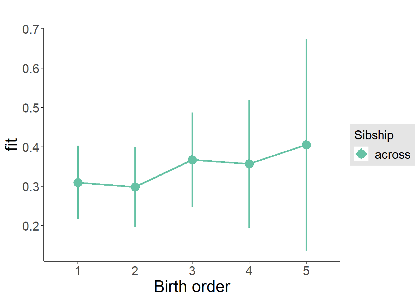
Add Interaction
Model Summary
m4_interaction = update(m3_birthorder_nonlinear, formula = . ~ . - birth_order_nonlinear - sibling_count + count_birth_order)
tidy(m4_interaction, conf.int = T, conf.level = 0.995)| effect | group | term | estimate | std.error | statistic | df | p.value | conf.low | conf.high |
|---|---|---|---|---|---|---|---|---|---|
| fixed | NA | (Intercept) | -6.366 | 4.173 | -1.526 | 2237 | 0.1273 | -18.08 | 5.347 |
| fixed | NA | poly(age, 3, raw = TRUE)1 | 0.717 | 0.436 | 1.645 | 2233 | 0.1002 | -0.5068 | 1.941 |
| fixed | NA | poly(age, 3, raw = TRUE)2 | -0.02474 | 0.01497 | -1.653 | 2230 | 0.09846 | -0.06675 | 0.01727 |
| fixed | NA | poly(age, 3, raw = TRUE)3 | 0.000277 | 0.0001689 | 1.64 | 2226 | 0.1011 | -0.0001971 | 0.0007511 |
| fixed | NA | male | 0.01205 | 0.03248 | 0.3709 | 2356 | 0.7107 | -0.07913 | 0.1032 |
| fixed | NA | count_birth_order2/2 | -0.0718 | 0.0659 | -1.089 | 1888 | 0.2761 | -0.2568 | 0.1132 |
| fixed | NA | count_birth_order1/3 | -0.04571 | 0.0628 | -0.7279 | 2500 | 0.4667 | -0.222 | 0.1306 |
| fixed | NA | count_birth_order2/3 | 0.03087 | 0.06934 | 0.4452 | 2535 | 0.6562 | -0.1638 | 0.2255 |
| fixed | NA | count_birth_order3/3 | -0.01001 | 0.07506 | -0.1334 | 2531 | 0.8939 | -0.2207 | 0.2007 |
| fixed | NA | count_birth_order1/4 | -0.1066 | 0.074 | -1.441 | 2530 | 0.1497 | -0.3143 | 0.1011 |
| fixed | NA | count_birth_order2/4 | -0.1273 | 0.07535 | -1.689 | 2531 | 0.09131 | -0.3388 | 0.08424 |
| fixed | NA | count_birth_order3/4 | -0.1199 | 0.07649 | -1.567 | 2521 | 0.1173 | -0.3346 | 0.09486 |
| fixed | NA | count_birth_order4/4 | -0.0405 | 0.08201 | -0.4938 | 2530 | 0.6215 | -0.2707 | 0.1897 |
| fixed | NA | count_birth_order1/5 | -0.2444 | 0.09518 | -2.568 | 2531 | 0.0103 | -0.5116 | 0.02279 |
| fixed | NA | count_birth_order2/5 | -0.3341 | 0.1005 | -3.323 | 2493 | 0.0009026 | -0.6164 | -0.0519 |
| fixed | NA | count_birth_order3/5 | 0.01908 | 0.09128 | 0.2091 | 2497 | 0.8344 | -0.2371 | 0.2753 |
| fixed | NA | count_birth_order4/5 | -0.2035 | 0.09196 | -2.213 | 2502 | 0.02699 | -0.4617 | 0.05464 |
| fixed | NA | count_birth_order5/5 | -0.1077 | 0.09939 | -1.083 | 2491 | 0.2788 | -0.3867 | 0.1713 |
| ran_pars | mother_pidlink | sd__(Intercept) | 0.474 | NA | NA | NA | NA | NA | NA |
| ran_pars | Residual | sd__Observation | 0.7045 | NA | NA | NA | NA | NA | NA |
Coefficient Plot
plot_birthorder(m4_interaction)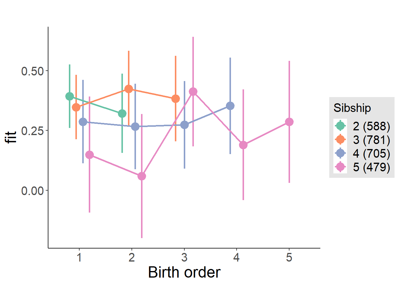
Model Comparison
###### Model 1 - Model 2
anova(m1_covariates_only, m2_birthorder_linear, m3_birthorder_nonlinear, m4_interaction)
## refitting model(s) with ML (instead of REML)| Df | AIC | BIC | logLik | deviance | Chisq | Chi Df | Pr(>Chisq) |
|---|---|---|---|---|---|---|---|
| 10 | 6332 | 6390 | -3156 | 6312 | NA | NA | NA |
| 11 | 6332 | 6396 | -3155 | 6310 | 1.626 | 1 | 0.2023 |
| 14 | 6337 | 6419 | -3154 | 6309 | 1.335 | 3 | 0.7207 |
| 20 | 6336 | 6453 | -3148 | 6296 | 12.39 | 6 | 0.05381 |
Compare birth order specifications
library(coefplot)
multiplot(outcome_naive_m1, outcome_preg_m1, outcome_uterus_m1, outcome_parental_m1, dodgeHeight = 0.6,
          intercept = FALSE)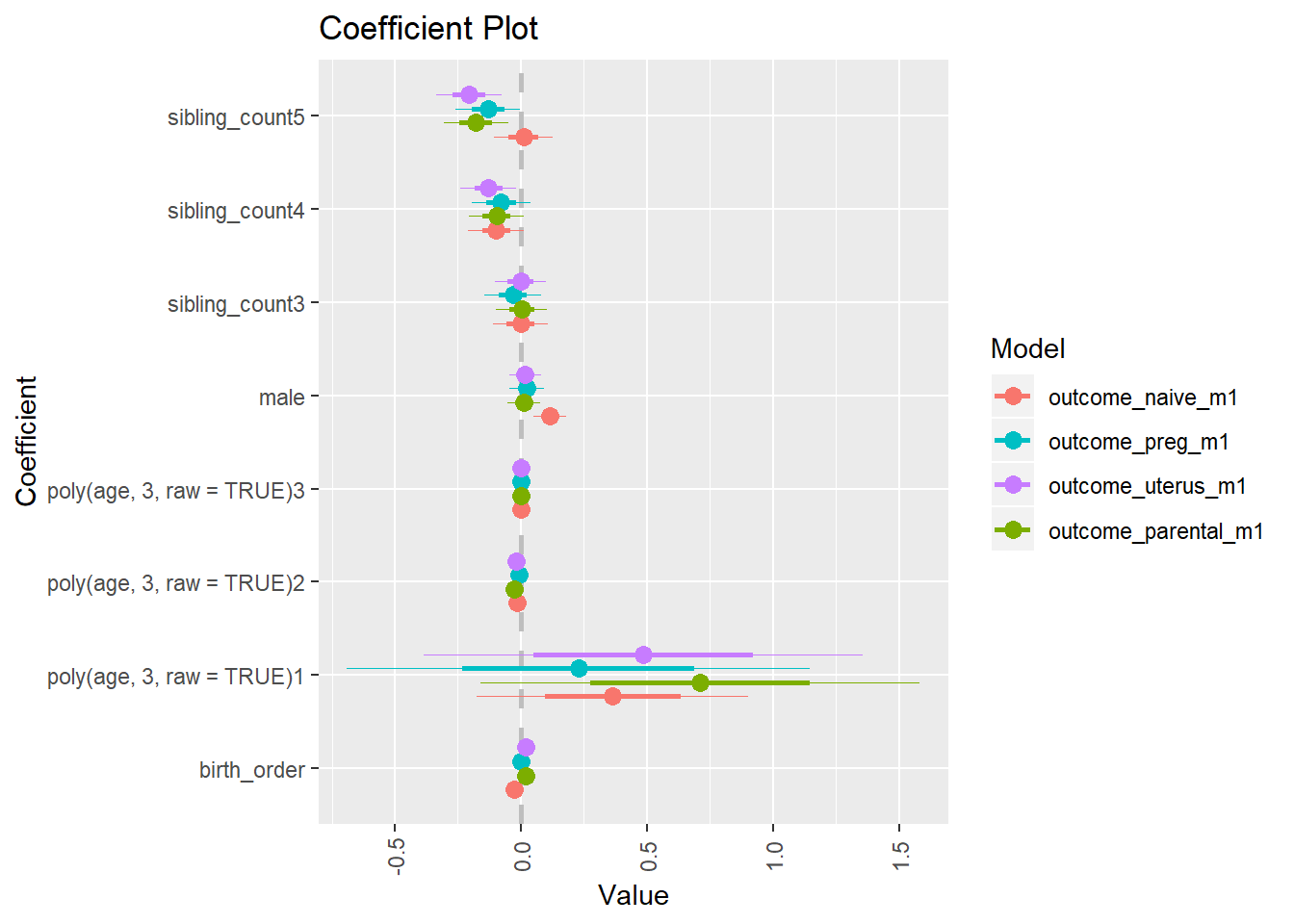
g-factor 2007 young
birthorder <- birthorder %>% mutate(outcome = g_factor_2007_young)
model = lmer(outcome ~ birth_order + poly(age, 3, raw = TRUE) + male + sibling_count + (1 | mother_pidlink),
                   data = birthorder)
compare_birthorder_specs(model)
Naive birth order
outcome_naive_m1 <- update(m2_birthorder_linear, data = birthorder %>%
                     mutate(sibling_count = sibling_count_naive_factor,
                            birth_order_nonlinear = birthorder_naive_factor,
                            birth_order = birthorder_naive,
                            count_birth_order = count_birthorder_naive) %>%
                     filter(sibling_count != "1"))
compare_models_markdown(outcome_naive_m1)
Basic Model
Model Summary
m1_covariates_only <- update(m2_birthorder_linear, formula = . ~ . - birth_order)
tidy(m1_covariates_only, conf.int = T, conf.level = 0.995)| effect | group | term | estimate | std.error | statistic | df | p.value | conf.low | conf.high |
|---|---|---|---|---|---|---|---|---|---|
| fixed | NA | (Intercept) | -7.324 | 0.5196 | -14.1 | 4623 | 3.293e-44 | -8.783 | -5.866 |
| fixed | NA | poly(age, 3, raw = TRUE)1 | 0.8042 | 0.06916 | 11.63 | 4758 | 7.745e-31 | 0.6101 | 0.9984 |
| fixed | NA | poly(age, 3, raw = TRUE)2 | -0.02602 | 0.002968 | -8.766 | 4905 | 2.507e-18 | -0.03435 | -0.01769 |
| fixed | NA | poly(age, 3, raw = TRUE)3 | 0.0002514 | 0.0000416 | 6.042 | 4961 | 0.000000001634 | 0.0001346 | 0.0003681 |
| fixed | NA | male | -0.0007239 | 0.02439 | -0.02969 | 4521 | 0.9763 | -0.06918 | 0.06773 |
| fixed | NA | sibling_count3 | -0.01199 | 0.03865 | -0.3102 | 3499 | 0.7564 | -0.1205 | 0.0965 |
| fixed | NA | sibling_count4 | -0.149 | 0.03954 | -3.768 | 3309 | 0.0001672 | -0.26 | -0.03801 |
| fixed | NA | sibling_count5 | -0.1275 | 0.04271 | -2.984 | 3095 | 0.002865 | -0.2474 | -0.00757 |
| ran_pars | mother_pidlink | sd__(Intercept) | 0.5178 | NA | NA | NA | NA | NA | NA |
| ran_pars | Residual | sd__Observation | 0.7313 | NA | NA | NA | NA | NA | NA |
Coefficient Plot
plot(allEffects(m1_covariates_only, confidence.level = 0.995))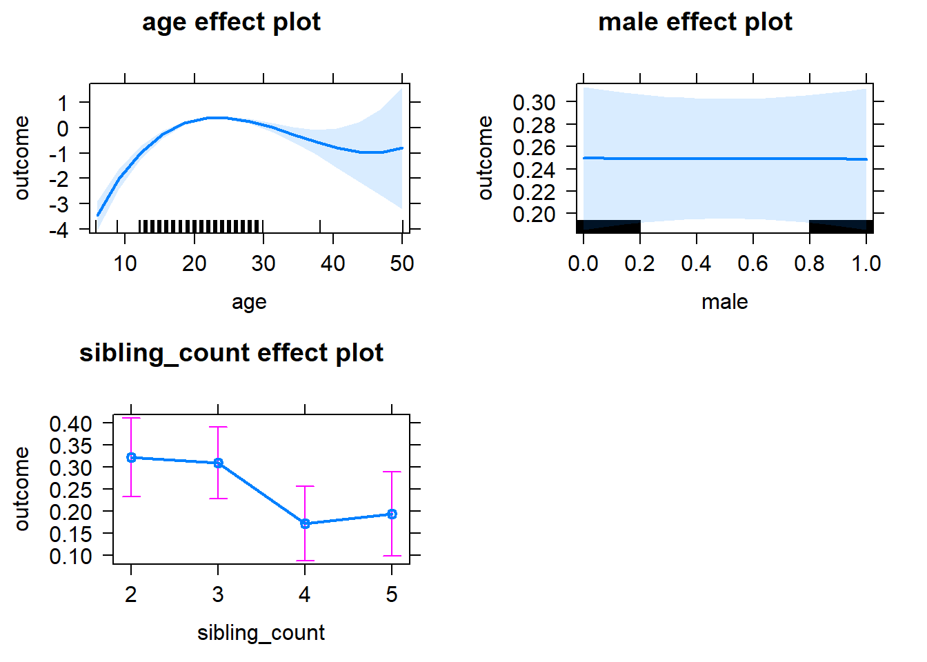
Add Birth Order Linear
Model Summary
tidy(m2_birthorder_linear, conf.int = T, conf.level = 0.995)| effect | group | term | estimate | std.error | statistic | df | p.value | conf.low | conf.high |
|---|---|---|---|---|---|---|---|---|---|
| fixed | NA | (Intercept) | -7.402 | 0.5202 | -14.23 | 4621 | 5.464e-45 | -8.862 | -5.941 |
| fixed | NA | birth_order | 0.03096 | 0.01203 | 2.574 | 4570 | 0.01007 | -0.002797 | 0.06472 |
| fixed | NA | poly(age, 3, raw = TRUE)1 | 0.8073 | 0.06914 | 11.68 | 4755 | 4.49e-31 | 0.6132 | 1.001 |
| fixed | NA | poly(age, 3, raw = TRUE)2 | -0.02608 | 0.002966 | -8.791 | 4903 | 2.02e-18 | -0.0344 | -0.01775 |
| fixed | NA | poly(age, 3, raw = TRUE)3 | 0.0002518 | 0.00004158 | 6.056 | 4960 | 0.000000001499 | 0.0001351 | 0.0003685 |
| fixed | NA | male | -0.001843 | 0.02438 | -0.07559 | 4523 | 0.9397 | -0.07028 | 0.06659 |
| fixed | NA | sibling_count3 | -0.02616 | 0.03901 | -0.6708 | 3533 | 0.5024 | -0.1357 | 0.08333 |
| fixed | NA | sibling_count4 | -0.1809 | 0.0414 | -4.369 | 3474 | 0.00001282 | -0.2971 | -0.06468 |
| fixed | NA | sibling_count5 | -0.1817 | 0.04758 | -3.818 | 3438 | 0.0001369 | -0.3152 | -0.0481 |
| ran_pars | mother_pidlink | sd__(Intercept) | 0.5166 | NA | NA | NA | NA | NA | NA |
| ran_pars | Residual | sd__Observation | 0.7313 | NA | NA | NA | NA | NA | NA |
Coefficient Plot
plot_birthorder2(m2_birthorder_linear, separate = FALSE)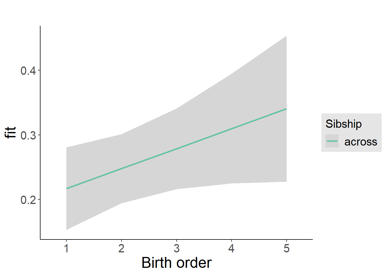
Add Birth Order Factor
Model Summary
m3_birthorder_nonlinear = update(m1_covariates_only, formula = . ~ . + birth_order_nonlinear)
tidy(m3_birthorder_nonlinear, conf.int = T, conf.level = 0.995)| effect | group | term | estimate | std.error | statistic | df | p.value | conf.low | conf.high |
|---|---|---|---|---|---|---|---|---|---|
| fixed | NA | (Intercept) | -7.436 | 0.5197 | -14.31 | 4629 | 1.775e-45 | -8.895 | -5.977 |
| fixed | NA | poly(age, 3, raw = TRUE)1 | 0.8136 | 0.0691 | 11.77 | 4756 | 1.444e-31 | 0.6197 | 1.008 |
| fixed | NA | poly(age, 3, raw = TRUE)2 | -0.02634 | 0.002964 | -8.884 | 4901 | 8.913e-19 | -0.03466 | -0.01801 |
| fixed | NA | poly(age, 3, raw = TRUE)3 | 0.000255 | 0.00004154 | 6.139 | 4957 | 0.0000000008979 | 0.0001384 | 0.0003716 |
| fixed | NA | male | -0.001712 | 0.02436 | -0.07031 | 4520 | 0.944 | -0.07008 | 0.06666 |
| fixed | NA | sibling_count3 | -0.01184 | 0.03936 | -0.3008 | 3628 | 0.7636 | -0.1223 | 0.09863 |
| fixed | NA | sibling_count4 | -0.173 | 0.04183 | -4.136 | 3584 | 0.0000361 | -0.2904 | -0.0556 |
| fixed | NA | sibling_count5 | -0.1748 | 0.04788 | -3.651 | 3466 | 0.0002648 | -0.3092 | -0.04042 |
| fixed | NA | birth_order_nonlinear2 | 0.08672 | 0.02855 | 3.038 | 3512 | 0.002401 | 0.006587 | 0.1668 |
| fixed | NA | birth_order_nonlinear3 | -0.005976 | 0.03524 | -0.1696 | 3790 | 0.8654 | -0.1049 | 0.09296 |
| fixed | NA | birth_order_nonlinear4 | 0.1429 | 0.04709 | 3.034 | 4106 | 0.002429 | 0.01069 | 0.2751 |
| fixed | NA | birth_order_nonlinear5 | 0.1438 | 0.06739 | 2.134 | 4326 | 0.03291 | -0.04536 | 0.333 |
| ran_pars | mother_pidlink | sd__(Intercept) | 0.5155 | NA | NA | NA | NA | NA | NA |
| ran_pars | Residual | sd__Observation | 0.7308 | NA | NA | NA | NA | NA | NA |
Coefficient Plot
plot_birthorder(m3_birthorder_nonlinear, separate = FALSE)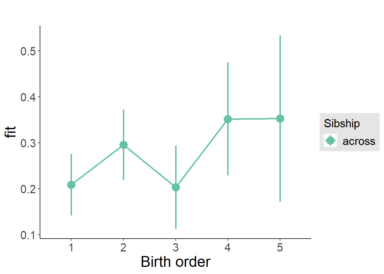
Add Interaction
Model Summary
m4_interaction = update(m3_birthorder_nonlinear, formula = . ~ . - birth_order_nonlinear - sibling_count + count_birth_order)
tidy(m4_interaction, conf.int = T, conf.level = 0.995)| effect | group | term | estimate | std.error | statistic | df | p.value | conf.low | conf.high |
|---|---|---|---|---|---|---|---|---|---|
| fixed | NA | (Intercept) | -7.43 | 0.5203 | -14.28 | 4624 | 2.692e-45 | -8.89 | -5.969 |
| fixed | NA | poly(age, 3, raw = TRUE)1 | 0.8131 | 0.06915 | 11.76 | 4749 | 1.751e-31 | 0.6189 | 1.007 |
| fixed | NA | poly(age, 3, raw = TRUE)2 | -0.02631 | 0.002966 | -8.869 | 4894 | 1.018e-18 | -0.03463 | -0.01798 |
| fixed | NA | poly(age, 3, raw = TRUE)3 | 0.0002546 | 0.00004157 | 6.126 | 4951 | 0.0000000009724 | 0.000138 | 0.0003713 |
| fixed | NA | male | -0.00201 | 0.02439 | -0.08244 | 4520 | 0.9343 | -0.07047 | 0.06645 |
| fixed | NA | count_birth_order2/2 | 0.07828 | 0.05326 | 1.47 | 3614 | 0.1417 | -0.07121 | 0.2278 |
| fixed | NA | count_birth_order1/3 | -0.01815 | 0.04764 | -0.3809 | 4857 | 0.7033 | -0.1519 | 0.1156 |
| fixed | NA | count_birth_order2/3 | 0.08603 | 0.05245 | 1.64 | 4951 | 0.101 | -0.06119 | 0.2332 |
| fixed | NA | count_birth_order3/3 | -0.03171 | 0.05884 | -0.5389 | 4943 | 0.59 | -0.1969 | 0.1335 |
| fixed | NA | count_birth_order1/4 | -0.186 | 0.05426 | -3.428 | 4940 | 0.0006124 | -0.3383 | -0.03371 |
| fixed | NA | count_birth_order2/4 | -0.0982 | 0.05542 | -1.772 | 4952 | 0.07645 | -0.2538 | 0.05736 |
| fixed | NA | count_birth_order3/4 | -0.1839 | 0.05789 | -3.178 | 4922 | 0.001494 | -0.3464 | -0.02145 |
| fixed | NA | count_birth_order4/4 | 0.001654 | 0.06316 | 0.02619 | 4903 | 0.9791 | -0.1756 | 0.1789 |
| fixed | NA | count_birth_order1/5 | -0.1567 | 0.06592 | -2.376 | 4943 | 0.01752 | -0.3417 | 0.02838 |
| fixed | NA | count_birth_order2/5 | -0.09442 | 0.06949 | -1.359 | 4853 | 0.1743 | -0.2895 | 0.1006 |
| fixed | NA | count_birth_order3/5 | -0.1626 | 0.06617 | -2.458 | 4848 | 0.01401 | -0.3484 | 0.0231 |
| fixed | NA | count_birth_order4/5 | -0.07784 | 0.06944 | -1.121 | 4820 | 0.2623 | -0.2728 | 0.1171 |
| fixed | NA | count_birth_order5/5 | -0.03441 | 0.06756 | -0.5094 | 4919 | 0.6105 | -0.224 | 0.1552 |
| ran_pars | mother_pidlink | sd__(Intercept) | 0.5145 | NA | NA | NA | NA | NA | NA |
| ran_pars | Residual | sd__Observation | 0.7318 | NA | NA | NA | NA | NA | NA |
Coefficient Plot
plot_birthorder(m4_interaction)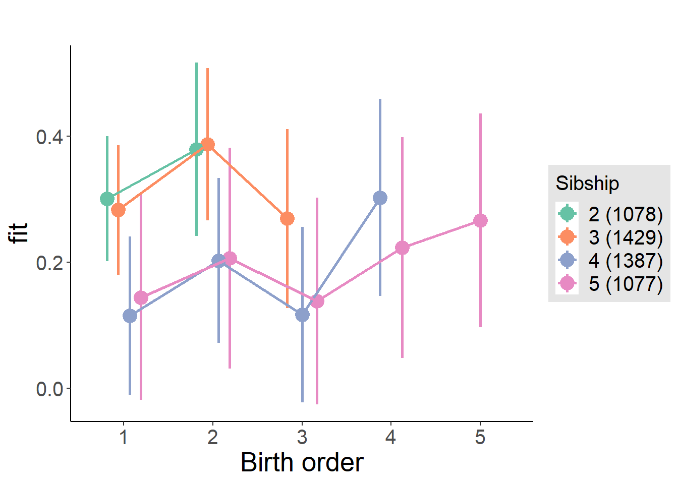
Model Comparison
###### Model 1 - Model 2
anova(m1_covariates_only, m2_birthorder_linear, m3_birthorder_nonlinear, m4_interaction)
## refitting model(s) with ML (instead of REML)| Df | AIC | BIC | logLik | deviance | Chisq | Chi Df | Pr(>Chisq) |
|---|---|---|---|---|---|---|---|
| 10 | 12822 | 12887 | -6401 | 12802 | NA | NA | NA |
| 11 | 12818 | 12889 | -6398 | 12796 | 6.635 | 1 | 0.009998 |
| 14 | 12810 | 12901 | -6391 | 12782 | 13.72 | 3 | 0.003312 |
| 20 | 12820 | 12950 | -6390 | 12780 | 1.632 | 6 | 0.9502 |
Maternal birth order
outcome_uterus_m1 <- update(m2_birthorder_linear, data = birthorder %>%
                     mutate(sibling_count = sibling_count_uterus_alive_factor,
                            birth_order_nonlinear = birthorder_uterus_alive_factor,
                            birth_order = birthorder_uterus_alive,
                            count_birth_order = count_birthorder_uterus_alive) %>%
                     filter(sibling_count != "1"))
compare_models_markdown(outcome_uterus_m1)
Basic Model
Model Summary
m1_covariates_only <- update(m2_birthorder_linear, formula = . ~ . - birth_order)
tidy(m1_covariates_only, conf.int = T, conf.level = 0.995)| effect | group | term | estimate | std.error | statistic | df | p.value | conf.low | conf.high |
|---|---|---|---|---|---|---|---|---|---|
| fixed | NA | (Intercept) | -6.328 | 1.241 | -5.1 | 3363 | 0.0000003579 | -9.81 | -2.845 |
| fixed | NA | poly(age, 3, raw = TRUE)1 | 0.639 | 0.1897 | 3.368 | 3342 | 0.0007666 | 0.1064 | 1.172 |
| fixed | NA | poly(age, 3, raw = TRUE)2 | -0.01717 | 0.009434 | -1.82 | 3326 | 0.06879 | -0.04365 | 0.009308 |
| fixed | NA | poly(age, 3, raw = TRUE)3 | 0.000104 | 0.0001526 | 0.6816 | 3314 | 0.4955 | -0.0003244 | 0.0005325 |
| fixed | NA | male | -0.03967 | 0.02524 | -1.572 | 4096 | 0.116 | -0.1105 | 0.03117 |
| fixed | NA | sibling_count3 | -0.0009547 | 0.03506 | -0.02723 | 3129 | 0.9783 | -0.09938 | 0.09747 |
| fixed | NA | sibling_count4 | -0.1098 | 0.03972 | -2.764 | 2845 | 0.00575 | -0.2213 | 0.001717 |
| fixed | NA | sibling_count5 | -0.183 | 0.04801 | -3.811 | 2737 | 0.0001413 | -0.3178 | -0.04822 |
| ran_pars | mother_pidlink | sd__(Intercept) | 0.5065 | NA | NA | NA | NA | NA | NA |
| ran_pars | Residual | sd__Observation | 0.7103 | NA | NA | NA | NA | NA | NA |
Coefficient Plot
plot(allEffects(m1_covariates_only, confidence.level = 0.995))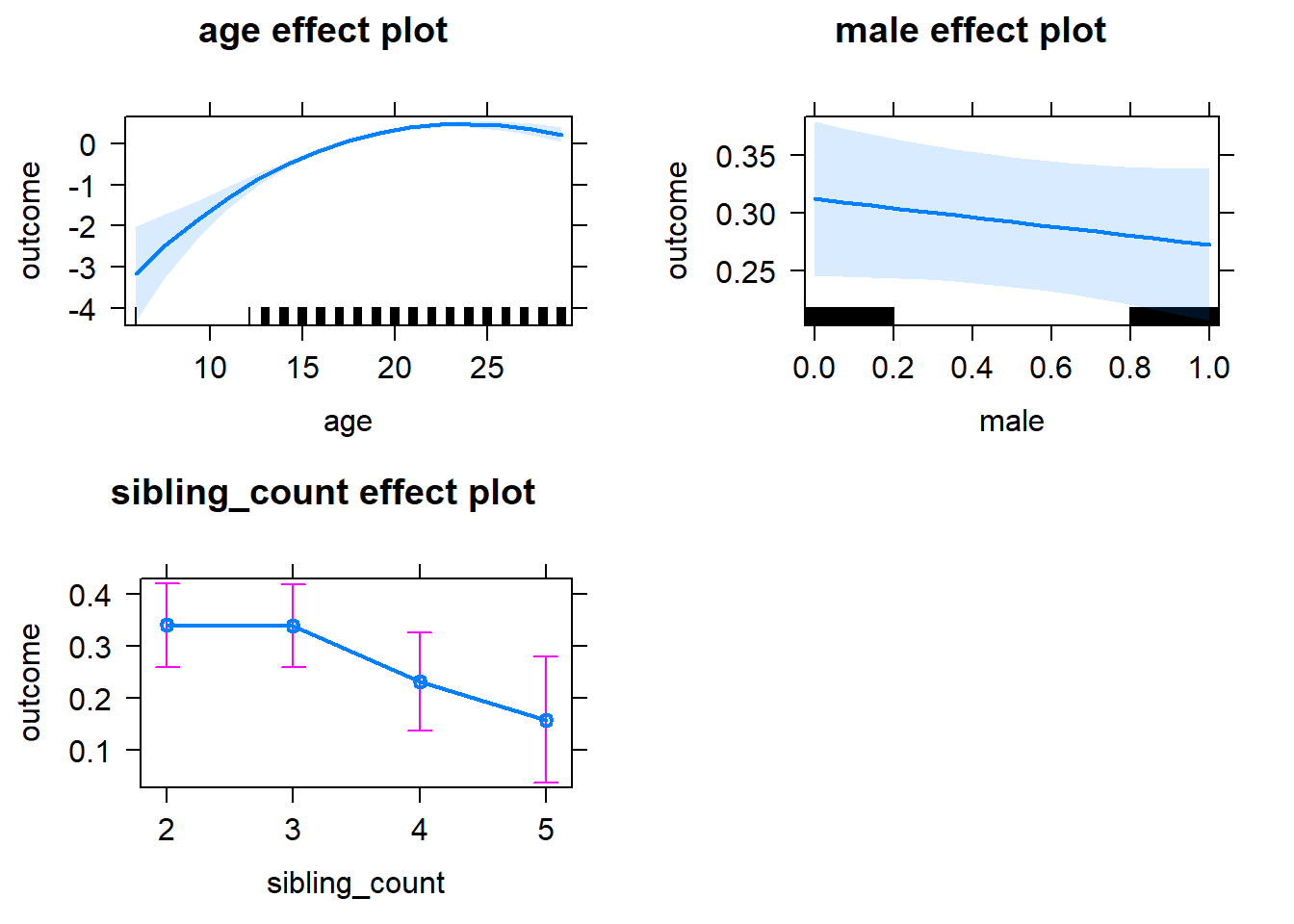
Add Birth Order Linear
Model Summary
tidy(m2_birthorder_linear, conf.int = T, conf.level = 0.995)| effect | group | term | estimate | std.error | statistic | df | p.value | conf.low | conf.high |
|---|---|---|---|---|---|---|---|---|---|
| fixed | NA | (Intercept) | -6.51 | 1.244 | -5.233 | 3370 | 0.000000177 | -10 | -3.018 |
| fixed | NA | birth_order | 0.02758 | 0.01385 | 1.992 | 4280 | 0.04648 | -0.01129 | 0.06646 |
| fixed | NA | poly(age, 3, raw = TRUE)1 | 0.6595 | 0.19 | 3.471 | 3343 | 0.0005256 | 0.1261 | 1.193 |
| fixed | NA | poly(age, 3, raw = TRUE)2 | -0.01813 | 0.009446 | -1.919 | 3325 | 0.05501 | -0.04465 | 0.008384 |
| fixed | NA | poly(age, 3, raw = TRUE)3 | 0.0001192 | 0.0001528 | 0.7801 | 3313 | 0.4354 | -0.0003098 | 0.0005482 |
| fixed | NA | male | -0.04046 | 0.02524 | -1.603 | 4099 | 0.109 | -0.1113 | 0.03038 |
| fixed | NA | sibling_count3 | -0.01434 | 0.03568 | -0.4019 | 3177 | 0.6878 | -0.1145 | 0.08581 |
| fixed | NA | sibling_count4 | -0.1424 | 0.04293 | -3.316 | 3063 | 0.0009224 | -0.2629 | -0.02187 |
| fixed | NA | sibling_count5 | -0.2388 | 0.05555 | -4.299 | 3155 | 0.0000177 | -0.3947 | -0.08287 |
| ran_pars | mother_pidlink | sd__(Intercept) | 0.5052 | NA | NA | NA | NA | NA | NA |
| ran_pars | Residual | sd__Observation | 0.7107 | NA | NA | NA | NA | NA | NA |
Coefficient Plot
plot_birthorder2(m2_birthorder_linear, separate = FALSE)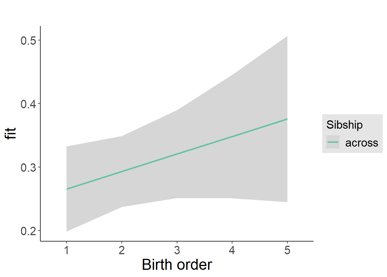
Add Birth Order Factor
Model Summary
m3_birthorder_nonlinear = update(m1_covariates_only, formula = . ~ . + birth_order_nonlinear)
tidy(m3_birthorder_nonlinear, conf.int = T, conf.level = 0.995)| effect | group | term | estimate | std.error | statistic | df | p.value | conf.low | conf.high |
|---|---|---|---|---|---|---|---|---|---|
| fixed | NA | (Intercept) | -6.548 | 1.244 | -5.262 | 3374 | 0.0000001512 | -10.04 | -3.055 |
| fixed | NA | poly(age, 3, raw = TRUE)1 | 0.6687 | 0.1902 | 3.516 | 3348 | 0.000444 | 0.1348 | 1.203 |
| fixed | NA | poly(age, 3, raw = TRUE)2 | -0.01858 | 0.009455 | -1.965 | 3331 | 0.04946 | -0.04512 | 0.007958 |
| fixed | NA | poly(age, 3, raw = TRUE)3 | 0.0001263 | 0.000153 | 0.8259 | 3320 | 0.4089 | -0.0003031 | 0.0005557 |
| fixed | NA | male | -0.04067 | 0.02525 | -1.611 | 4097 | 0.1073 | -0.1115 | 0.03021 |
| fixed | NA | sibling_count3 | -0.007151 | 0.03623 | -0.1974 | 3294 | 0.8436 | -0.1089 | 0.09456 |
| fixed | NA | sibling_count4 | -0.1343 | 0.04367 | -3.075 | 3159 | 0.002122 | -0.2569 | -0.01171 |
| fixed | NA | sibling_count5 | -0.2444 | 0.05724 | -4.271 | 3232 | 0.00002006 | -0.4051 | -0.08376 |
| fixed | NA | birth_order_nonlinear2 | 0.04433 | 0.02868 | 1.546 | 2993 | 0.1222 | -0.03616 | 0.1248 |
| fixed | NA | birth_order_nonlinear3 | 0.02522 | 0.03858 | 0.6539 | 3589 | 0.5132 | -0.08306 | 0.1335 |
| fixed | NA | birth_order_nonlinear4 | 0.08059 | 0.05323 | 1.514 | 3993 | 0.1301 | -0.06881 | 0.23 |
| fixed | NA | birth_order_nonlinear5 | 0.1653 | 0.08324 | 1.986 | 3964 | 0.04713 | -0.06837 | 0.3989 |
| ran_pars | mother_pidlink | sd__(Intercept) | 0.5046 | NA | NA | NA | NA | NA | NA |
| ran_pars | Residual | sd__Observation | 0.7111 | NA | NA | NA | NA | NA | NA |
Coefficient Plot
plot_birthorder(m3_birthorder_nonlinear, separate = FALSE)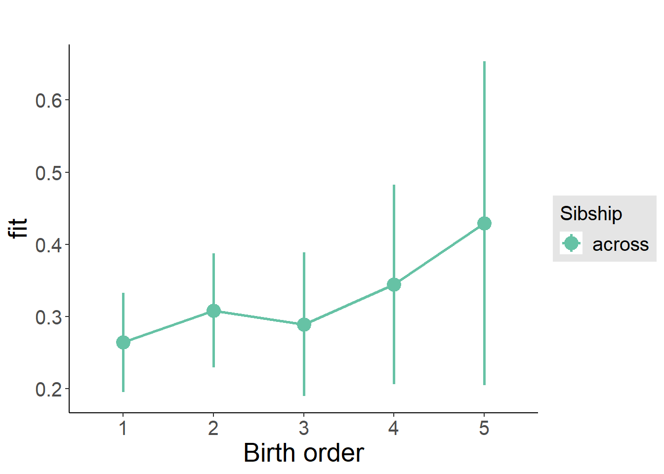
Add Interaction
Model Summary
m4_interaction = update(m3_birthorder_nonlinear, formula = . ~ . - birth_order_nonlinear - sibling_count + count_birth_order)
tidy(m4_interaction, conf.int = T, conf.level = 0.995)| effect | group | term | estimate | std.error | statistic | df | p.value | conf.low | conf.high |
|---|---|---|---|---|---|---|---|---|---|
| fixed | NA | (Intercept) | -6.542 | 1.245 | -5.253 | 3372 | 0.0000001586 | -10.04 | -3.046 |
| fixed | NA | poly(age, 3, raw = TRUE)1 | 0.6681 | 0.1903 | 3.51 | 3346 | 0.0004542 | 0.1338 | 1.202 |
| fixed | NA | poly(age, 3, raw = TRUE)2 | -0.01856 | 0.009462 | -1.961 | 3329 | 0.04995 | -0.04512 | 0.008004 |
| fixed | NA | poly(age, 3, raw = TRUE)3 | 0.0001262 | 0.0001531 | 0.8243 | 3317 | 0.4098 | -0.0003035 | 0.0005559 |
| fixed | NA | male | -0.04045 | 0.02528 | -1.6 | 4091 | 0.1096 | -0.1114 | 0.03051 |
| fixed | NA | count_birth_order2/2 | 0.03333 | 0.04609 | 0.7233 | 3275 | 0.4696 | -0.09604 | 0.1627 |
| fixed | NA | count_birth_order1/3 | -0.03346 | 0.04428 | -0.7557 | 4369 | 0.4499 | -0.1577 | 0.09083 |
| fixed | NA | count_birth_order2/3 | 0.06004 | 0.04812 | 1.248 | 4420 | 0.2121 | -0.07502 | 0.1951 |
| fixed | NA | count_birth_order3/3 | 0.0239 | 0.05367 | 0.4453 | 4420 | 0.6561 | -0.1267 | 0.1745 |
| fixed | NA | count_birth_order1/4 | -0.1253 | 0.05955 | -2.104 | 4422 | 0.03541 | -0.2925 | 0.04185 |
| fixed | NA | count_birth_order2/4 | -0.1411 | 0.05944 | -2.374 | 4382 | 0.01762 | -0.308 | 0.02572 |
| fixed | NA | count_birth_order3/4 | -0.1075 | 0.06195 | -1.735 | 4290 | 0.08282 | -0.2814 | 0.06642 |
| fixed | NA | count_birth_order4/4 | -0.0287 | 0.06155 | -0.4663 | 4419 | 0.641 | -0.2015 | 0.1441 |
| fixed | NA | count_birth_order1/5 | -0.1659 | 0.08989 | -1.845 | 4342 | 0.06507 | -0.4182 | 0.08645 |
| fixed | NA | count_birth_order2/5 | -0.1693 | 0.09476 | -1.786 | 4084 | 0.0741 | -0.4353 | 0.09671 |
| fixed | NA | count_birth_order3/5 | -0.2539 | 0.08351 | -3.041 | 4194 | 0.002373 | -0.4883 | -0.01954 |
| fixed | NA | count_birth_order4/5 | -0.2206 | 0.07848 | -2.811 | 4295 | 0.004959 | -0.4409 | -0.0003212 |
| fixed | NA | count_birth_order5/5 | -0.08879 | 0.07603 | -1.168 | 4407 | 0.2429 | -0.3022 | 0.1246 |
| ran_pars | mother_pidlink | sd__(Intercept) | 0.5053 | NA | NA | NA | NA | NA | NA |
| ran_pars | Residual | sd__Observation | 0.7109 | NA | NA | NA | NA | NA | NA |
Coefficient Plot
plot_birthorder(m4_interaction)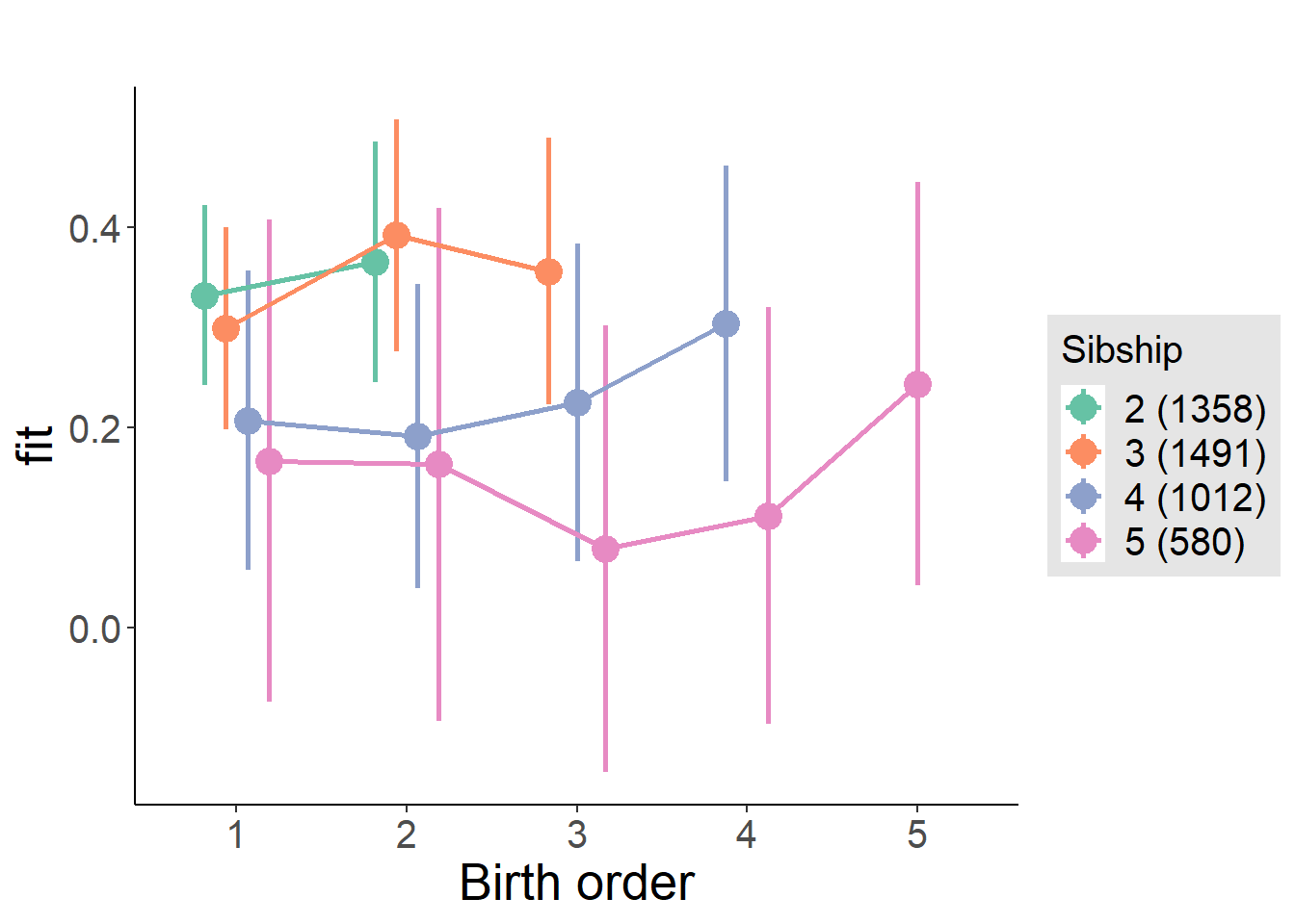
Model Comparison
###### Model 1 - Model 2
anova(m1_covariates_only, m2_birthorder_linear, m3_birthorder_nonlinear, m4_interaction)
## refitting model(s) with ML (instead of REML)| Df | AIC | BIC | logLik | deviance | Chisq | Chi Df | Pr(>Chisq) |
|---|---|---|---|---|---|---|---|
| 10 | 11231 | 11295 | -5606 | 11211 | NA | NA | NA |
| 11 | 11229 | 11299 | -5604 | 11207 | 3.971 | 1 | 0.04628 |
| 14 | 11233 | 11323 | -5603 | 11205 | 2.088 | 3 | 0.5544 |
| 20 | 11241 | 11369 | -5600 | 11201 | 4.469 | 6 | 0.6135 |
Maternal pregnancy order
outcome_preg_m1 <- update(m2_birthorder_linear, data = birthorder %>%
  mutate(sibling_count = sibling_count_uterus_preg_factor,
         birth_order_nonlinear = birthorder_uterus_preg_factor,
         birth_order = birthorder_uterus_preg,
         count_birth_order = count_birthorder_uterus_preg
         ) %>%
    filter(sibling_count != "1"))
compare_models_markdown(outcome_preg_m1)
Basic Model
Model Summary
m1_covariates_only <- update(m2_birthorder_linear, formula = . ~ . - birth_order)
tidy(m1_covariates_only, conf.int = T, conf.level = 0.995)| effect | group | term | estimate | std.error | statistic | df | p.value | conf.low | conf.high |
|---|---|---|---|---|---|---|---|---|---|
| fixed | NA | (Intercept) | -6.168 | 1.273 | -4.846 | 3077 | 0.000001323 | -9.741 | -2.595 |
| fixed | NA | poly(age, 3, raw = TRUE)1 | 0.6238 | 0.1948 | 3.203 | 3055 | 0.001374 | 0.07712 | 1.171 |
| fixed | NA | poly(age, 3, raw = TRUE)2 | -0.01682 | 0.009694 | -1.735 | 3040 | 0.08282 | -0.04403 | 0.01039 |
| fixed | NA | poly(age, 3, raw = TRUE)3 | 0.0001046 | 0.000157 | 0.6661 | 3027 | 0.5054 | -0.0003362 | 0.0005453 |
| fixed | NA | male | -0.03772 | 0.02602 | -1.45 | 3792 | 0.1472 | -0.1108 | 0.03532 |
| fixed | NA | sibling_count3 | -0.02109 | 0.03765 | -0.5602 | 2973 | 0.5754 | -0.1268 | 0.08459 |
| fixed | NA | sibling_count4 | -0.08749 | 0.04106 | -2.131 | 2746 | 0.03319 | -0.2027 | 0.02776 |
| fixed | NA | sibling_count5 | -0.1585 | 0.04644 | -3.413 | 2690 | 0.0006516 | -0.2889 | -0.02815 |
| ran_pars | mother_pidlink | sd__(Intercept) | 0.5117 | NA | NA | NA | NA | NA | NA |
| ran_pars | Residual | sd__Observation | 0.7037 | NA | NA | NA | NA | NA | NA |
Coefficient Plot
plot(allEffects(m1_covariates_only, confidence.level = 0.995))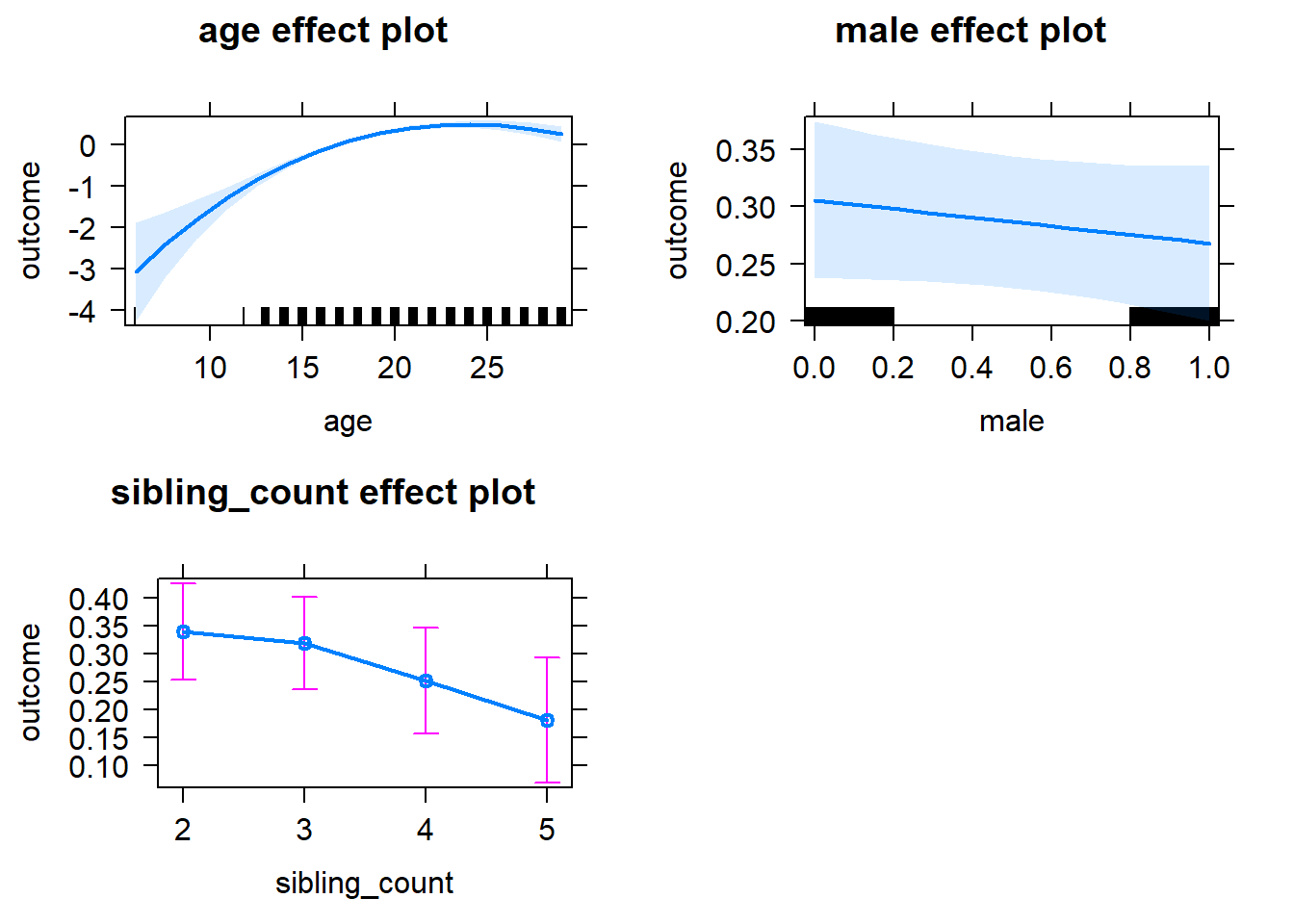
Add Birth Order Linear
Model Summary
tidy(m2_birthorder_linear, conf.int = T, conf.level = 0.995)| effect | group | term | estimate | std.error | statistic | df | p.value | conf.low | conf.high |
|---|---|---|---|---|---|---|---|---|---|
| fixed | NA | (Intercept) | -6.331 | 1.276 | -4.962 | 3084 | 0.0000007361 | -9.912 | -2.749 |
| fixed | NA | birth_order | 0.02546 | 0.01379 | 1.846 | 4030 | 0.06496 | -0.01326 | 0.06418 |
| fixed | NA | poly(age, 3, raw = TRUE)1 | 0.6421 | 0.195 | 3.292 | 3057 | 0.001005 | 0.09466 | 1.19 |
| fixed | NA | poly(age, 3, raw = TRUE)2 | -0.01768 | 0.009706 | -1.822 | 3040 | 0.06857 | -0.04493 | 0.009562 |
| fixed | NA | poly(age, 3, raw = TRUE)3 | 0.0001185 | 0.0001572 | 0.7535 | 3027 | 0.4512 | -0.0003228 | 0.0005597 |
| fixed | NA | male | -0.03847 | 0.02602 | -1.478 | 3795 | 0.1395 | -0.1115 | 0.03458 |
| fixed | NA | sibling_count3 | -0.03373 | 0.03824 | -0.8819 | 3005 | 0.3779 | -0.1411 | 0.07362 |
| fixed | NA | sibling_count4 | -0.1159 | 0.04382 | -2.645 | 2917 | 0.008213 | -0.2389 | 0.007101 |
| fixed | NA | sibling_count5 | -0.2061 | 0.05308 | -3.883 | 2997 | 0.0001056 | -0.3551 | -0.05709 |
| ran_pars | mother_pidlink | sd__(Intercept) | 0.5105 | NA | NA | NA | NA | NA | NA |
| ran_pars | Residual | sd__Observation | 0.7041 | NA | NA | NA | NA | NA | NA |
Coefficient Plot
plot_birthorder2(m2_birthorder_linear, separate = FALSE)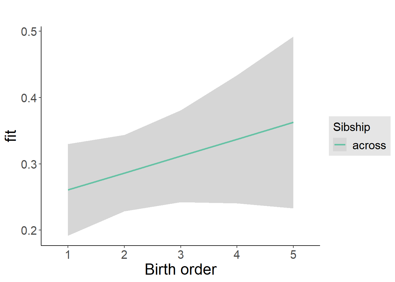
Add Birth Order Factor
Model Summary
m3_birthorder_nonlinear = update(m1_covariates_only, formula = . ~ . + birth_order_nonlinear)
tidy(m3_birthorder_nonlinear, conf.int = T, conf.level = 0.995)| effect | group | term | estimate | std.error | statistic | df | p.value | conf.low | conf.high |
|---|---|---|---|---|---|---|---|---|---|
| fixed | NA | (Intercept) | -6.391 | 1.275 | -5.011 | 3084 | 0.0000005722 | -9.97 | -2.811 |
| fixed | NA | poly(age, 3, raw = TRUE)1 | 0.6528 | 0.1951 | 3.346 | 3057 | 0.0008285 | 0.1052 | 1.2 |
| fixed | NA | poly(age, 3, raw = TRUE)2 | -0.0182 | 0.009708 | -1.875 | 3040 | 0.06088 | -0.04545 | 0.009048 |
| fixed | NA | poly(age, 3, raw = TRUE)3 | 0.0001266 | 0.0001572 | 0.8051 | 3028 | 0.4208 | -0.0003148 | 0.000568 |
| fixed | NA | male | -0.03784 | 0.02602 | -1.454 | 3789 | 0.1459 | -0.1109 | 0.03519 |
| fixed | NA | sibling_count3 | -0.02436 | 0.03878 | -0.6281 | 3104 | 0.53 | -0.1332 | 0.08451 |
| fixed | NA | sibling_count4 | -0.1044 | 0.04446 | -2.348 | 3010 | 0.01894 | -0.2292 | 0.02041 |
| fixed | NA | sibling_count5 | -0.2034 | 0.05402 | -3.765 | 3019 | 0.0001696 | -0.3551 | -0.05176 |
| fixed | NA | birth_order_nonlinear2 | 0.0732 | 0.02976 | 2.46 | 2812 | 0.01396 | -0.01033 | 0.1567 |
| fixed | NA | birth_order_nonlinear3 | 0.009629 | 0.03919 | 0.2457 | 3372 | 0.8059 | -0.1004 | 0.1196 |
| fixed | NA | birth_order_nonlinear4 | 0.07597 | 0.05328 | 1.426 | 3667 | 0.154 | -0.07358 | 0.2255 |
| fixed | NA | birth_order_nonlinear5 | 0.1518 | 0.07995 | 1.898 | 3844 | 0.05773 | -0.07266 | 0.3762 |
| ran_pars | mother_pidlink | sd__(Intercept) | 0.5108 | NA | NA | NA | NA | NA | NA |
| ran_pars | Residual | sd__Observation | 0.7035 | NA | NA | NA | NA | NA | NA |
Coefficient Plot
plot_birthorder(m3_birthorder_nonlinear, separate = FALSE)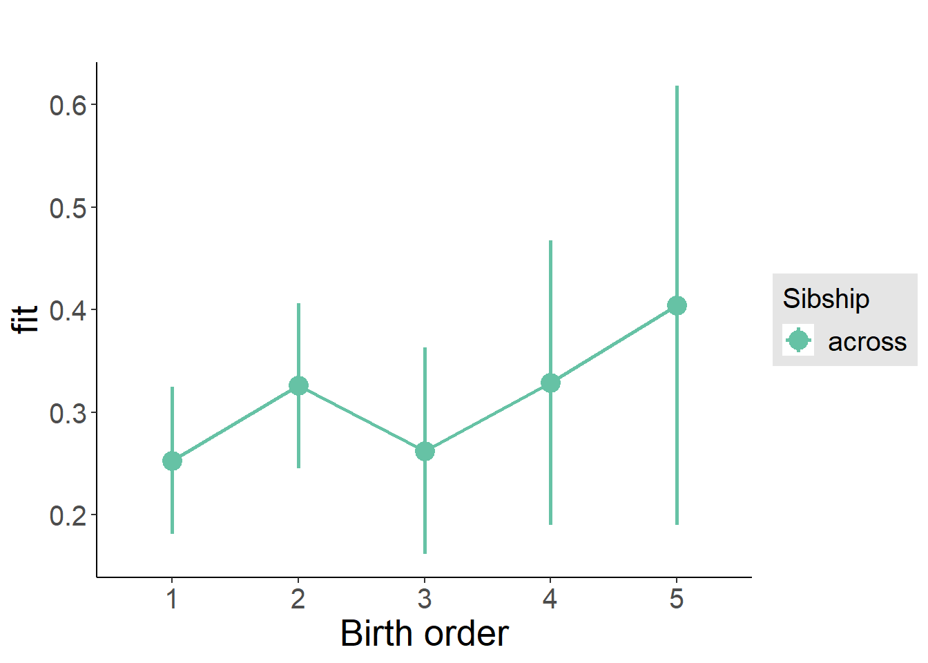
Add Interaction
Model Summary
m4_interaction = update(m3_birthorder_nonlinear, formula = . ~ . - birth_order_nonlinear - sibling_count + count_birth_order)
tidy(m4_interaction, conf.int = T, conf.level = 0.995)| effect | group | term | estimate | std.error | statistic | df | p.value | conf.low | conf.high |
|---|---|---|---|---|---|---|---|---|---|
| fixed | NA | (Intercept) | -6.391 | 1.274 | -5.015 | 3073 | 0.0000005613 | -9.968 | -2.814 |
| fixed | NA | poly(age, 3, raw = TRUE)1 | 0.6531 | 0.195 | 3.35 | 3048 | 0.0008193 | 0.1058 | 1.2 |
| fixed | NA | poly(age, 3, raw = TRUE)2 | -0.01827 | 0.009703 | -1.883 | 3031 | 0.05977 | -0.04551 | 0.008964 |
| fixed | NA | poly(age, 3, raw = TRUE)3 | 0.0001289 | 0.0001572 | 0.8201 | 3019 | 0.4122 | -0.0003123 | 0.00057 |
| fixed | NA | male | -0.03926 | 0.02602 | -1.509 | 3780 | 0.1314 | -0.1123 | 0.03378 |
| fixed | NA | count_birth_order2/2 | 0.08644 | 0.05025 | 1.72 | 3010 | 0.08548 | -0.05461 | 0.2275 |
| fixed | NA | count_birth_order1/3 | -0.04782 | 0.04758 | -1.005 | 4085 | 0.3149 | -0.1814 | 0.08574 |
| fixed | NA | count_birth_order2/3 | 0.06277 | 0.05105 | 1.23 | 4128 | 0.2189 | -0.08053 | 0.2061 |
| fixed | NA | count_birth_order3/3 | 0.02804 | 0.05732 | 0.4891 | 4124 | 0.6248 | -0.1329 | 0.189 |
| fixed | NA | count_birth_order1/4 | -0.09395 | 0.05961 | -1.576 | 4129 | 0.1151 | -0.2613 | 0.07338 |
| fixed | NA | count_birth_order2/4 | -0.06605 | 0.06009 | -1.099 | 4099 | 0.2718 | -0.2347 | 0.1026 |
| fixed | NA | count_birth_order3/4 | -0.1119 | 0.06309 | -1.774 | 4013 | 0.0761 | -0.289 | 0.06515 |
| fixed | NA | count_birth_order4/4 | 0.03027 | 0.06473 | 0.4677 | 4121 | 0.64 | -0.1514 | 0.212 |
| fixed | NA | count_birth_order1/5 | -0.07302 | 0.08077 | -0.904 | 4075 | 0.366 | -0.2998 | 0.1537 |
| fixed | NA | count_birth_order2/5 | -0.1053 | 0.08165 | -1.29 | 3971 | 0.1971 | -0.3346 | 0.1239 |
| fixed | NA | count_birth_order3/5 | -0.2344 | 0.07788 | -3.009 | 3952 | 0.002635 | -0.453 | -0.01575 |
| fixed | NA | count_birth_order4/5 | -0.2159 | 0.07831 | -2.757 | 3923 | 0.005858 | -0.4357 | 0.003906 |
| fixed | NA | count_birth_order5/5 | -0.05716 | 0.07509 | -0.7612 | 4117 | 0.4466 | -0.268 | 0.1536 |
| ran_pars | mother_pidlink | sd__(Intercept) | 0.5131 | NA | NA | NA | NA | NA | NA |
| ran_pars | Residual | sd__Observation | 0.7019 | NA | NA | NA | NA | NA | NA |
Coefficient Plot
plot_birthorder(m4_interaction)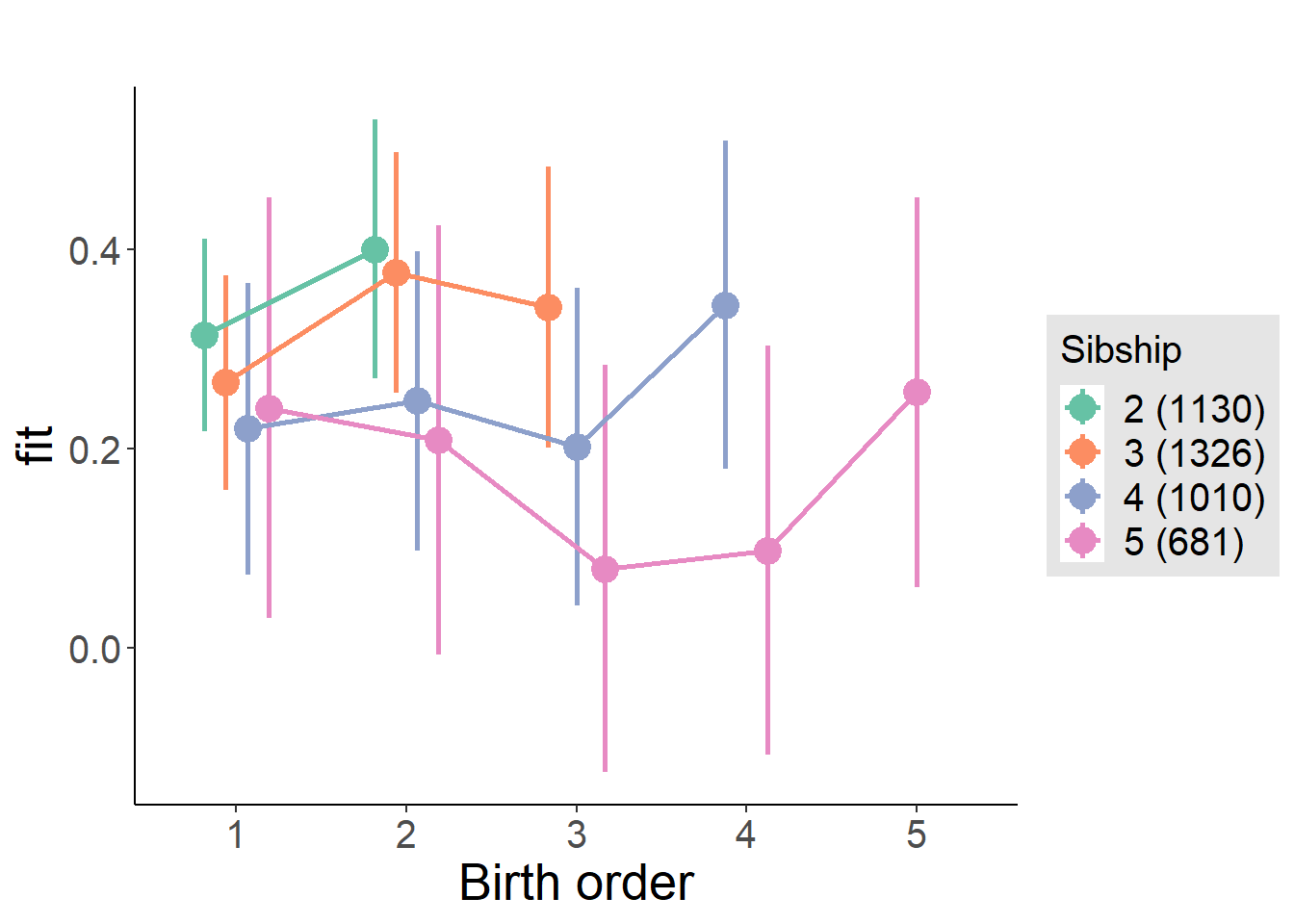
Model Comparison
###### Model 1 - Model 2
anova(m1_covariates_only, m2_birthorder_linear, m3_birthorder_nonlinear, m4_interaction)
## refitting model(s) with ML (instead of REML)| Df | AIC | BIC | logLik | deviance | Chisq | Chi Df | Pr(>Chisq) |
|---|---|---|---|---|---|---|---|
| 10 | 10463 | 10526 | -5221 | 10443 | NA | NA | NA |
| 11 | 10462 | 10531 | -5220 | 10440 | 3.413 | 1 | 0.0647 |
| 14 | 10461 | 10550 | -5217 | 10433 | 6.292 | 3 | 0.09825 |
| 20 | 10465 | 10591 | -5212 | 10425 | 8.753 | 6 | 0.188 |
Parental full sibling order
outcome_parental_m1 <- update(m2_birthorder_linear, data = birthorder %>%
  mutate(sibling_count = sibling_count_genes_factor,
         birth_order_nonlinear = birthorder_genes_factor,
         birth_order = birthorder_genes,
         count_birth_order = count_birthorder_genes
         ) %>%
      filter(sibling_count != "1"))
compare_models_markdown(outcome_parental_m1)
Basic Model
Model Summary
m1_covariates_only <- update(m2_birthorder_linear, formula = . ~ . - birth_order)
tidy(m1_covariates_only, conf.int = T, conf.level = 0.995)| effect | group | term | estimate | std.error | statistic | df | p.value | conf.low | conf.high |
|---|---|---|---|---|---|---|---|---|---|
| fixed | NA | (Intercept) | -5.829 | 1.258 | -4.634 | 3264 | 0.000003724 | -9.36 | -2.298 |
| fixed | NA | poly(age, 3, raw = TRUE)1 | 0.56 | 0.1923 | 2.912 | 3243 | 0.003611 | 0.02026 | 1.1 |
| fixed | NA | poly(age, 3, raw = TRUE)2 | -0.01319 | 0.009558 | -1.38 | 3229 | 0.1677 | -0.04002 | 0.01364 |
| fixed | NA | poly(age, 3, raw = TRUE)3 | 0.00003789 | 0.0001546 | 0.2451 | 3217 | 0.8064 | -0.0003961 | 0.0004719 |
| fixed | NA | male | -0.04295 | 0.02561 | -1.677 | 4000 | 0.09358 | -0.1148 | 0.02893 |
| fixed | NA | sibling_count3 | 0.01545 | 0.0354 | 0.4364 | 3066 | 0.6626 | -0.08393 | 0.1148 |
| fixed | NA | sibling_count4 | -0.09473 | 0.04028 | -2.352 | 2790 | 0.01876 | -0.2078 | 0.01835 |
| fixed | NA | sibling_count5 | -0.1953 | 0.05039 | -3.875 | 2713 | 0.0001089 | -0.3367 | -0.05383 |
| ran_pars | mother_pidlink | sd__(Intercept) | 0.5188 | NA | NA | NA | NA | NA | NA |
| ran_pars | Residual | sd__Observation | 0.713 | NA | NA | NA | NA | NA | NA |
Coefficient Plot
plot(allEffects(m1_covariates_only, confidence.level = 0.995))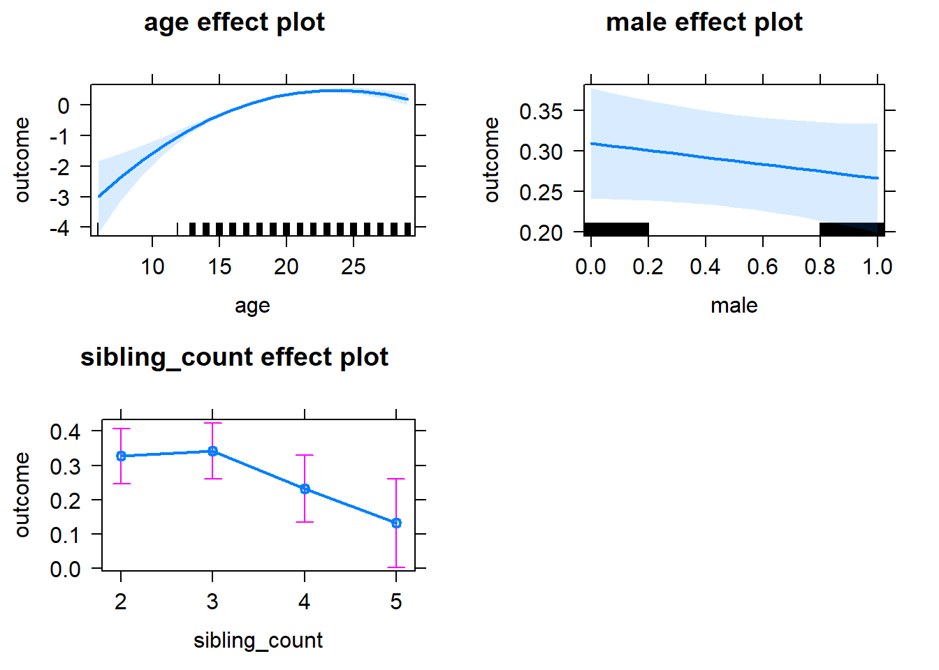
Add Birth Order Linear
Model Summary
tidy(m2_birthorder_linear, conf.int = T, conf.level = 0.995)| effect | group | term | estimate | std.error | statistic | df | p.value | conf.low | conf.high |
|---|---|---|---|---|---|---|---|---|---|
| fixed | NA | (Intercept) | -6.028 | 1.261 | -4.779 | 3271 | 0.00000184 | -9.569 | -2.487 |
| fixed | NA | birth_order | 0.02919 | 0.01417 | 2.061 | 4172 | 0.03941 | -0.01057 | 0.06895 |
| fixed | NA | poly(age, 3, raw = TRUE)1 | 0.5828 | 0.1926 | 3.026 | 3243 | 0.002495 | 0.04223 | 1.123 |
| fixed | NA | poly(age, 3, raw = TRUE)2 | -0.01427 | 0.009571 | -1.491 | 3226 | 0.1362 | -0.04113 | 0.0126 |
| fixed | NA | poly(age, 3, raw = TRUE)3 | 0.00005509 | 0.0001548 | 0.3559 | 3215 | 0.7219 | -0.0003795 | 0.0004896 |
| fixed | NA | male | -0.04357 | 0.0256 | -1.702 | 4001 | 0.0889 | -0.1154 | 0.0283 |
| fixed | NA | sibling_count3 | 0.00164 | 0.03601 | 0.04555 | 3112 | 0.9637 | -0.09945 | 0.1027 |
| fixed | NA | sibling_count4 | -0.1295 | 0.04365 | -2.967 | 3013 | 0.003032 | -0.252 | -0.006979 |
| fixed | NA | sibling_count5 | -0.2529 | 0.0576 | -4.391 | 3096 | 0.00001166 | -0.4146 | -0.09125 |
| ran_pars | mother_pidlink | sd__(Intercept) | 0.5178 | NA | NA | NA | NA | NA | NA |
| ran_pars | Residual | sd__Observation | 0.7132 | NA | NA | NA | NA | NA | NA |
Coefficient Plot
plot_birthorder2(m2_birthorder_linear, separate = FALSE)
Add Birth Order Factor
Model Summary
m3_birthorder_nonlinear = update(m1_covariates_only, formula = . ~ . + birth_order_nonlinear)
tidy(m3_birthorder_nonlinear, conf.int = T, conf.level = 0.995)| effect | group | term | estimate | std.error | statistic | df | p.value | conf.low | conf.high |
|---|---|---|---|---|---|---|---|---|---|
| fixed | NA | (Intercept) | -6.023 | 1.263 | -4.77 | 3276 | 0.000001918 | -9.567 | -2.479 |
| fixed | NA | poly(age, 3, raw = TRUE)1 | 0.5852 | 0.1929 | 3.034 | 3249 | 0.002433 | 0.04376 | 1.127 |
| fixed | NA | poly(age, 3, raw = TRUE)2 | -0.01436 | 0.009586 | -1.498 | 3232 | 0.1342 | -0.04127 | 0.01255 |
| fixed | NA | poly(age, 3, raw = TRUE)3 | 0.00005626 | 0.000155 | 0.3629 | 3221 | 0.7167 | -0.0003789 | 0.0004915 |
| fixed | NA | male | -0.04382 | 0.02562 | -1.711 | 3998 | 0.08724 | -0.1157 | 0.02809 |
| fixed | NA | sibling_count3 | 0.001778 | 0.03659 | 0.04861 | 3227 | 0.9612 | -0.1009 | 0.1045 |
| fixed | NA | sibling_count4 | -0.1253 | 0.04444 | -2.821 | 3113 | 0.004825 | -0.2501 | -0.0006004 |
| fixed | NA | sibling_count5 | -0.2469 | 0.05971 | -4.135 | 3179 | 0.00003646 | -0.4145 | -0.07928 |
| fixed | NA | birth_order_nonlinear2 | 0.04764 | 0.02886 | 1.651 | 2904 | 0.09895 | -0.03338 | 0.1287 |
| fixed | NA | birth_order_nonlinear3 | 0.05963 | 0.03912 | 1.524 | 3454 | 0.1275 | -0.05018 | 0.1694 |
| fixed | NA | birth_order_nonlinear4 | 0.07538 | 0.05463 | 1.38 | 3879 | 0.1677 | -0.07796 | 0.2287 |
| fixed | NA | birth_order_nonlinear5 | 0.1165 | 0.08926 | 1.305 | 3927 | 0.1921 | -0.1341 | 0.367 |
| ran_pars | mother_pidlink | sd__(Intercept) | 0.5175 | NA | NA | NA | NA | NA | NA |
| ran_pars | Residual | sd__Observation | 0.7137 | NA | NA | NA | NA | NA | NA |
Coefficient Plot
plot_birthorder(m3_birthorder_nonlinear, separate = FALSE)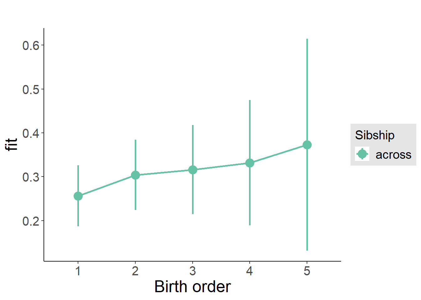
Add Interaction
Model Summary
m4_interaction = update(m3_birthorder_nonlinear, formula = . ~ . - birth_order_nonlinear - sibling_count + count_birth_order)
tidy(m4_interaction, conf.int = T, conf.level = 0.995)| effect | group | term | estimate | std.error | statistic | df | p.value | conf.low | conf.high |
|---|---|---|---|---|---|---|---|---|---|
| fixed | NA | (Intercept) | -6.022 | 1.263 | -4.767 | 3274 | 0.000001953 | -9.569 | -2.476 |
| fixed | NA | poly(age, 3, raw = TRUE)1 | 0.5849 | 0.193 | 3.03 | 3248 | 0.002465 | 0.04303 | 1.127 |
| fixed | NA | poly(age, 3, raw = TRUE)2 | -0.01432 | 0.009593 | -1.493 | 3230 | 0.1355 | -0.04125 | 0.01261 |
| fixed | NA | poly(age, 3, raw = TRUE)3 | 0.00005547 | 0.0001552 | 0.3575 | 3218 | 0.7207 | -0.0003801 | 0.000491 |
| fixed | NA | male | -0.04315 | 0.02566 | -1.682 | 3994 | 0.09265 | -0.1152 | 0.02886 |
| fixed | NA | count_birth_order2/2 | 0.03616 | 0.04536 | 0.7973 | 3146 | 0.4254 | -0.09116 | 0.1635 |
| fixed | NA | count_birth_order1/3 | -0.02526 | 0.04458 | -0.5665 | 4304 | 0.5711 | -0.1504 | 0.09989 |
| fixed | NA | count_birth_order2/3 | 0.08174 | 0.04901 | 1.668 | 4355 | 0.09543 | -0.05584 | 0.2193 |
| fixed | NA | count_birth_order3/3 | 0.05704 | 0.0542 | 1.052 | 4353 | 0.2927 | -0.0951 | 0.2092 |
| fixed | NA | count_birth_order1/4 | -0.1136 | 0.06091 | -1.865 | 4357 | 0.06225 | -0.2846 | 0.05738 |
| fixed | NA | count_birth_order2/4 | -0.1328 | 0.06033 | -2.201 | 4317 | 0.02778 | -0.3021 | 0.03655 |
| fixed | NA | count_birth_order3/4 | -0.06945 | 0.06258 | -1.11 | 4208 | 0.2672 | -0.2451 | 0.1062 |
| fixed | NA | count_birth_order4/4 | -0.0207 | 0.06221 | -0.3327 | 4355 | 0.7394 | -0.1953 | 0.1539 |
| fixed | NA | count_birth_order1/5 | -0.1693 | 0.09198 | -1.84 | 4291 | 0.06581 | -0.4275 | 0.08893 |
| fixed | NA | count_birth_order2/5 | -0.2048 | 0.1015 | -2.017 | 3964 | 0.04375 | -0.4898 | 0.0802 |
| fixed | NA | count_birth_order3/5 | -0.1832 | 0.08841 | -2.072 | 4117 | 0.03835 | -0.4313 | 0.06501 |
| fixed | NA | count_birth_order4/5 | -0.2445 | 0.08348 | -2.929 | 4198 | 0.003423 | -0.4788 | -0.01015 |
| fixed | NA | count_birth_order5/5 | -0.1409 | 0.08145 | -1.73 | 4340 | 0.08375 | -0.3695 | 0.08774 |
| ran_pars | mother_pidlink | sd__(Intercept) | 0.5178 | NA | NA | NA | NA | NA | NA |
| ran_pars | Residual | sd__Observation | 0.7136 | NA | NA | NA | NA | NA | NA |
Coefficient Plot
plot_birthorder(m4_interaction)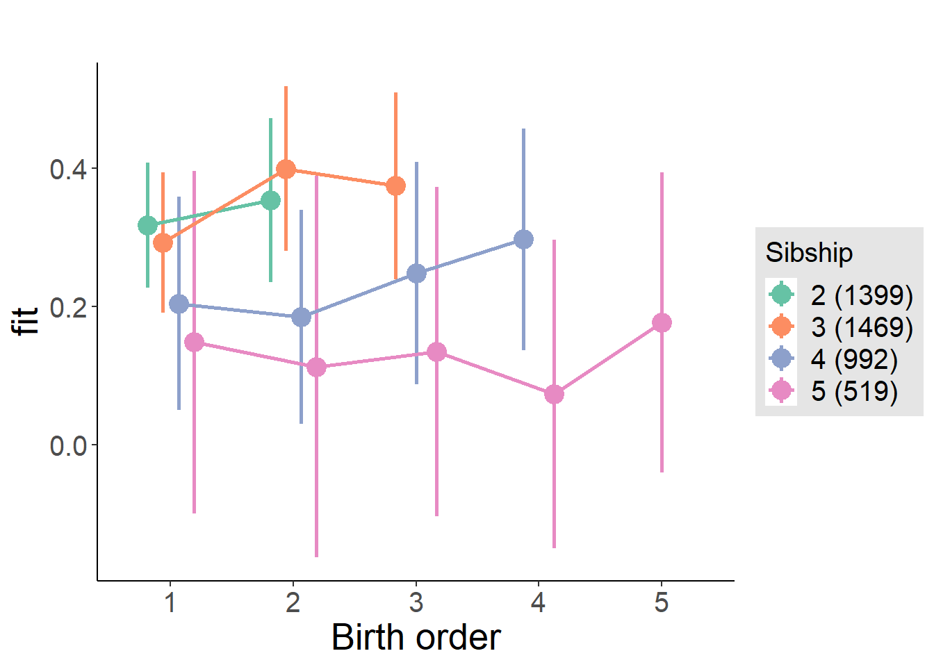
Model Comparison
###### Model 1 - Model 2
anova(m1_covariates_only, m2_birthorder_linear, m3_birthorder_nonlinear, m4_interaction)
## refitting model(s) with ML (instead of REML)| Df | AIC | BIC | logLik | deviance | Chisq | Chi Df | Pr(>Chisq) |
|---|---|---|---|---|---|---|---|
| 10 | 11157 | 11221 | -5569 | 11137 | NA | NA | NA |
| 11 | 11155 | 11225 | -5567 | 11133 | 4.252 | 1 | 0.0392 |
| 14 | 11161 | 11250 | -5566 | 11133 | 0.5888 | 3 | 0.899 |
| 20 | 11167 | 11295 | -5564 | 11127 | 5.03 | 6 | 0.54 |
Compare birth order specifications
library(coefplot)
multiplot(outcome_naive_m1, outcome_preg_m1, outcome_uterus_m1, outcome_parental_m1, dodgeHeight = 0.6,
          intercept = FALSE)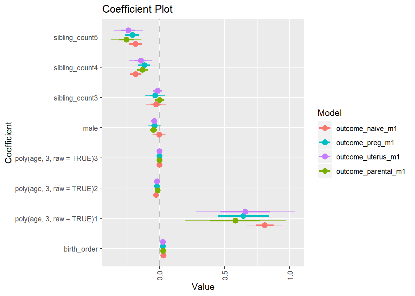
Raven 2015 old
birthorder <- birthorder %>% mutate(outcome = raven_2015_old)
model = lmer(outcome ~ birth_order + poly(age, 3, raw = TRUE) + male + sibling_count + (1 | mother_pidlink),
                   data = birthorder)
compare_birthorder_specs(model)
Naive birth order
outcome_naive_m1 <- update(m2_birthorder_linear, data = birthorder %>%
                     mutate(sibling_count = sibling_count_naive_factor,
                            birth_order_nonlinear = birthorder_naive_factor,
                            birth_order = birthorder_naive,
                            count_birth_order = count_birthorder_naive) %>%
                     filter(sibling_count != "1"))
compare_models_markdown(outcome_naive_m1)
Basic Model
Model Summary
m1_covariates_only <- update(m2_birthorder_linear, formula = . ~ . - birth_order)
tidy(m1_covariates_only, conf.int = T, conf.level = 0.995)| effect | group | term | estimate | std.error | statistic | df | p.value | conf.low | conf.high |
|---|---|---|---|---|---|---|---|---|---|
| fixed | NA | (Intercept) | -0.4153 | 0.1856 | -2.237 | 7051 | 0.02529 | -0.9363 | 0.1057 |
| fixed | NA | poly(age, 3, raw = TRUE)1 | 0.07945 | 0.01789 | 4.441 | 6992 | 0.000009113 | 0.02923 | 0.1297 |
| fixed | NA | poly(age, 3, raw = TRUE)2 | -0.002707 | 0.0005245 | -5.161 | 6891 | 0.0000002526 | -0.004179 | -0.001235 |
| fixed | NA | poly(age, 3, raw = TRUE)3 | 0.00001973 | 0.000004771 | 4.136 | 6792 | 0.00003577 | 0.000006341 | 0.00003313 |
| fixed | NA | male | 0.148 | 0.02101 | 7.044 | 6696 | 2.054e-12 | 0.08903 | 0.207 |
| fixed | NA | sibling_count3 | 0.02843 | 0.0322 | 0.8828 | 4908 | 0.3774 | -0.06196 | 0.1188 |
| fixed | NA | sibling_count4 | -0.009102 | 0.03344 | -0.2722 | 4522 | 0.7855 | -0.103 | 0.08477 |
| fixed | NA | sibling_count5 | 0.02765 | 0.0351 | 0.7878 | 4153 | 0.4308 | -0.07087 | 0.1262 |
| ran_pars | mother_pidlink | sd__(Intercept) | 0.4717 | NA | NA | NA | NA | NA | NA |
| ran_pars | Residual | sd__Observation | 0.7857 | NA | NA | NA | NA | NA | NA |
Coefficient Plot
plot(allEffects(m1_covariates_only, confidence.level = 0.995))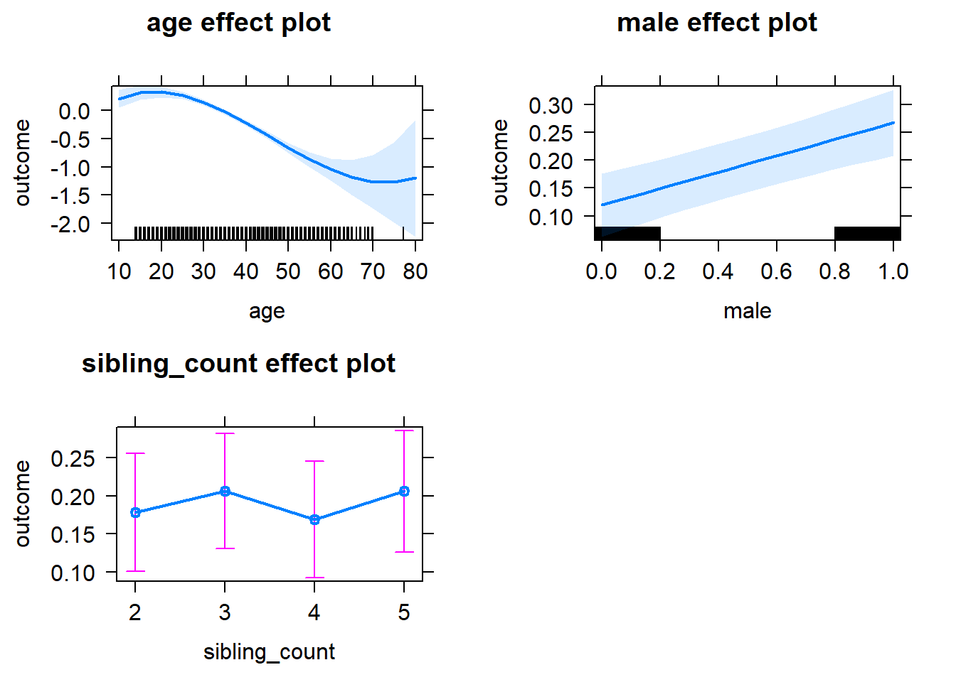
Add Birth Order Linear
Model Summary
tidy(m2_birthorder_linear, conf.int = T, conf.level = 0.995)| effect | group | term | estimate | std.error | statistic | df | p.value | conf.low | conf.high |
|---|---|---|---|---|---|---|---|---|---|
| fixed | NA | (Intercept) | -0.4193 | 0.1857 | -2.258 | 7039 | 0.02401 | -0.9406 | 0.1021 |
| fixed | NA | birth_order | 0.006446 | 0.01027 | 0.6279 | 5656 | 0.5301 | -0.02237 | 0.03527 |
| fixed | NA | poly(age, 3, raw = TRUE)1 | 0.07888 | 0.01792 | 4.403 | 7005 | 0.00001083 | 0.02859 | 0.1292 |
| fixed | NA | poly(age, 3, raw = TRUE)2 | -0.002691 | 0.0005251 | -5.125 | 6900 | 0.000000306 | -0.004165 | -0.001217 |
| fixed | NA | poly(age, 3, raw = TRUE)3 | 0.00001963 | 0.000004774 | 4.111 | 6797 | 0.00003979 | 0.000006228 | 0.00003303 |
| fixed | NA | male | 0.1479 | 0.02102 | 7.035 | 6693 | 2.184e-12 | 0.08886 | 0.2068 |
| fixed | NA | sibling_count3 | 0.02628 | 0.03238 | 0.8114 | 5017 | 0.4172 | -0.06462 | 0.1172 |
| fixed | NA | sibling_count4 | -0.01424 | 0.03443 | -0.4137 | 4974 | 0.6791 | -0.1109 | 0.0824 |
| fixed | NA | sibling_count5 | 0.01925 | 0.03757 | 0.5123 | 5064 | 0.6085 | -0.08621 | 0.1247 |
| ran_pars | mother_pidlink | sd__(Intercept) | 0.4717 | NA | NA | NA | NA | NA | NA |
| ran_pars | Residual | sd__Observation | 0.7858 | NA | NA | NA | NA | NA | NA |
Coefficient Plot
plot_birthorder2(m2_birthorder_linear, separate = FALSE)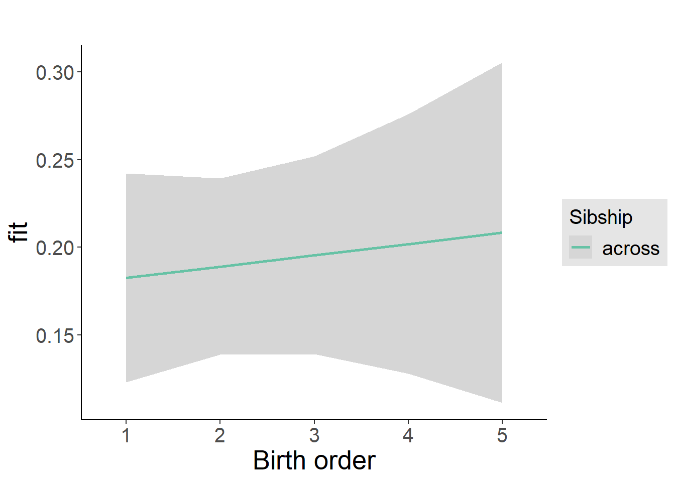
Add Birth Order Factor
Model Summary
m3_birthorder_nonlinear = update(m1_covariates_only, formula = . ~ . + birth_order_nonlinear)
tidy(m3_birthorder_nonlinear, conf.int = T, conf.level = 0.995)| effect | group | term | estimate | std.error | statistic | df | p.value | conf.low | conf.high |
|---|---|---|---|---|---|---|---|---|---|
| fixed | NA | (Intercept) | -0.4077 | 0.1861 | -2.191 | 7046 | 0.02851 | -0.93 | 0.1147 |
| fixed | NA | poly(age, 3, raw = TRUE)1 | 0.07889 | 0.01793 | 4.401 | 6990 | 0.00001093 | 0.02858 | 0.1292 |
| fixed | NA | poly(age, 3, raw = TRUE)2 | -0.002684 | 0.0005257 | -5.105 | 6872 | 0.0000003399 | -0.004159 | -0.001208 |
| fixed | NA | poly(age, 3, raw = TRUE)3 | 0.0000195 | 0.000004783 | 4.077 | 6753 | 0.00004613 | 0.000006074 | 0.00003292 |
| fixed | NA | male | 0.148 | 0.02101 | 7.046 | 6692 | 2.033e-12 | 0.08906 | 0.207 |
| fixed | NA | sibling_count3 | 0.02062 | 0.03277 | 0.6292 | 5198 | 0.5292 | -0.07136 | 0.1126 |
| fixed | NA | sibling_count4 | -0.009991 | 0.03485 | -0.2866 | 5171 | 0.7744 | -0.1078 | 0.08784 |
| fixed | NA | sibling_count5 | 0.01146 | 0.0378 | 0.3032 | 5200 | 0.7617 | -0.09465 | 0.1176 |
| fixed | NA | birth_order_nonlinear2 | -0.01535 | 0.02437 | -0.63 | 5626 | 0.5287 | -0.08375 | 0.05304 |
| fixed | NA | birth_order_nonlinear3 | 0.03391 | 0.03121 | 1.087 | 5409 | 0.2773 | -0.05369 | 0.1215 |
| fixed | NA | birth_order_nonlinear4 | -0.04011 | 0.04063 | -0.9872 | 5323 | 0.3236 | -0.1542 | 0.07394 |
| fixed | NA | birth_order_nonlinear5 | 0.09271 | 0.05926 | 1.565 | 5082 | 0.1177 | -0.07362 | 0.259 |
| ran_pars | mother_pidlink | sd__(Intercept) | 0.4708 | NA | NA | NA | NA | NA | NA |
| ran_pars | Residual | sd__Observation | 0.786 | NA | NA | NA | NA | NA | NA |
Coefficient Plot
plot_birthorder(m3_birthorder_nonlinear, separate = FALSE)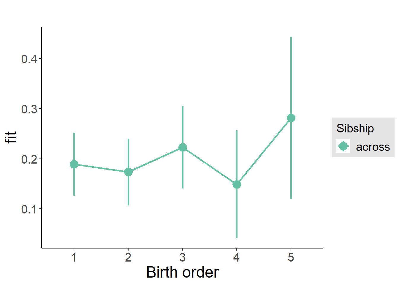
Add Interaction
Model Summary
m4_interaction = update(m3_birthorder_nonlinear, formula = . ~ . - birth_order_nonlinear - sibling_count + count_birth_order)
tidy(m4_interaction, conf.int = T, conf.level = 0.995)| effect | group | term | estimate | std.error | statistic | df | p.value | conf.low | conf.high |
|---|---|---|---|---|---|---|---|---|---|
| fixed | NA | (Intercept) | -0.3852 | 0.1864 | -2.066 | 7043 | 0.03884 | -0.9085 | 0.1381 |
| fixed | NA | poly(age, 3, raw = TRUE)1 | 0.07885 | 0.01793 | 4.399 | 6985 | 0.00001106 | 0.02853 | 0.1292 |
| fixed | NA | poly(age, 3, raw = TRUE)2 | -0.002669 | 0.0005257 | -5.078 | 6865 | 0.0000003922 | -0.004145 | -0.001194 |
| fixed | NA | poly(age, 3, raw = TRUE)3 | 0.00001926 | 0.000004784 | 4.027 | 6742 | 0.0000571 | 0.000005836 | 0.00003269 |
| fixed | NA | male | 0.1483 | 0.02102 | 7.057 | 6684 | 1.875e-12 | 0.08931 | 0.2073 |
| fixed | NA | count_birth_order2/2 | -0.08728 | 0.04168 | -2.094 | 5752 | 0.03628 | -0.2043 | 0.0297 |
| fixed | NA | count_birth_order1/3 | -0.00209 | 0.0411 | -0.05085 | 7026 | 0.9594 | -0.1175 | 0.1133 |
| fixed | NA | count_birth_order2/3 | -0.02197 | 0.04564 | -0.4814 | 7116 | 0.6303 | -0.1501 | 0.1061 |
| fixed | NA | count_birth_order3/3 | 0.0221 | 0.05101 | 0.4333 | 7133 | 0.6648 | -0.1211 | 0.1653 |
| fixed | NA | count_birth_order1/4 | -0.06028 | 0.04657 | -1.294 | 7115 | 0.1956 | -0.191 | 0.07044 |
| fixed | NA | count_birth_order2/4 | -0.01072 | 0.04913 | -0.2181 | 7135 | 0.8273 | -0.1486 | 0.1272 |
| fixed | NA | count_birth_order3/4 | -0.01018 | 0.05312 | -0.1917 | 7119 | 0.848 | -0.1593 | 0.1389 |
| fixed | NA | count_birth_order4/4 | -0.08644 | 0.05594 | -1.545 | 7096 | 0.1224 | -0.2435 | 0.0706 |
| fixed | NA | count_birth_order1/5 | -0.06351 | 0.05287 | -1.201 | 7136 | 0.2297 | -0.2119 | 0.0849 |
| fixed | NA | count_birth_order2/5 | -0.00108 | 0.05527 | -0.01954 | 7118 | 0.9844 | -0.1562 | 0.1541 |
| fixed | NA | count_birth_order3/5 | 0.03526 | 0.05691 | 0.6196 | 7090 | 0.5356 | -0.1245 | 0.195 |
| fixed | NA | count_birth_order4/5 | -0.04227 | 0.06011 | -0.7032 | 7037 | 0.4819 | -0.211 | 0.1265 |
| fixed | NA | count_birth_order5/5 | 0.07895 | 0.06157 | 1.282 | 7012 | 0.1998 | -0.09389 | 0.2518 |
| ran_pars | mother_pidlink | sd__(Intercept) | 0.471 | NA | NA | NA | NA | NA | NA |
| ran_pars | Residual | sd__Observation | 0.7859 | NA | NA | NA | NA | NA | NA |
Coefficient Plot
plot_birthorder(m4_interaction)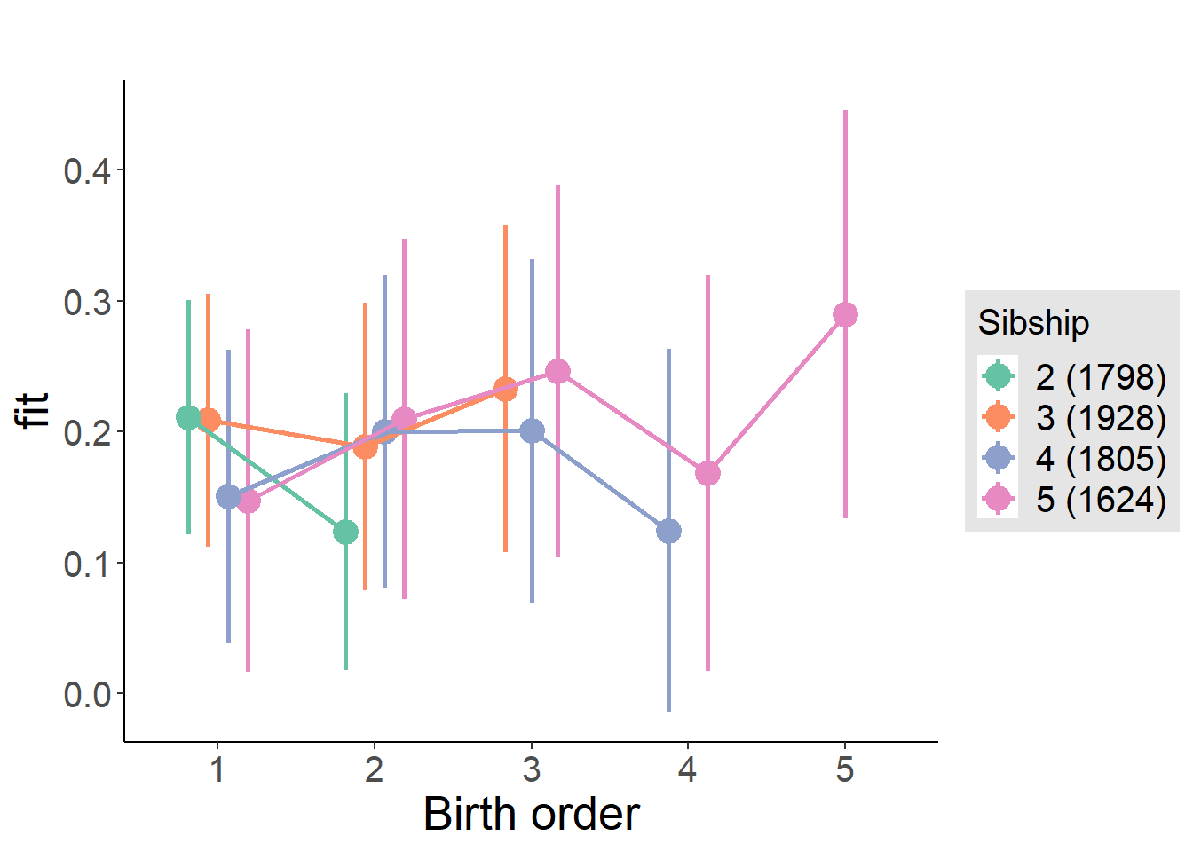
Model Comparison
###### Model 1 - Model 2
anova(m1_covariates_only, m2_birthorder_linear, m3_birthorder_nonlinear, m4_interaction)
## refitting model(s) with ML (instead of REML)| Df | AIC | BIC | logLik | deviance | Chisq | Chi Df | Pr(>Chisq) |
|---|---|---|---|---|---|---|---|
| 10 | 18847 | 18916 | -9414 | 18827 | NA | NA | NA |
| 11 | 18849 | 18924 | -9413 | 18827 | 0.3945 | 1 | 0.5299 |
| 14 | 18849 | 18945 | -9410 | 18821 | 6.299 | 3 | 0.09794 |
| 20 | 18854 | 18991 | -9407 | 18814 | 6.616 | 6 | 0.3578 |
Maternal birth order
outcome_uterus_m1 <- update(m2_birthorder_linear, data = birthorder %>%
                     mutate(sibling_count = sibling_count_uterus_alive_factor,
                            birth_order_nonlinear = birthorder_uterus_alive_factor,
                            birth_order = birthorder_uterus_alive,
                            count_birth_order = count_birthorder_uterus_alive) %>%
                     filter(sibling_count != "1"))
compare_models_markdown(outcome_uterus_m1)
Basic Model
Model Summary
m1_covariates_only <- update(m2_birthorder_linear, formula = . ~ . - birth_order)
tidy(m1_covariates_only, conf.int = T, conf.level = 0.995)| effect | group | term | estimate | std.error | statistic | df | p.value | conf.low | conf.high |
|---|---|---|---|---|---|---|---|---|---|
| fixed | NA | (Intercept) | 0.1652 | 0.4595 | 0.3595 | 4468 | 0.7192 | -1.125 | 1.455 |
| fixed | NA | poly(age, 3, raw = TRUE)1 | 0.003894 | 0.05367 | 0.07255 | 4478 | 0.9422 | -0.1468 | 0.1545 |
| fixed | NA | poly(age, 3, raw = TRUE)2 | 0.0007124 | 0.00198 | 0.3599 | 4488 | 0.719 | -0.004845 | 0.006269 |
| fixed | NA | poly(age, 3, raw = TRUE)3 | -0.00002249 | 0.00002321 | -0.9689 | 4496 | 0.3327 | -0.00008765 | 0.00004267 |
| fixed | NA | male | 0.07522 | 0.02458 | 3.061 | 4284 | 0.002223 | 0.006232 | 0.1442 |
| fixed | NA | sibling_count3 | 0.02922 | 0.03501 | 0.8345 | 3224 | 0.4041 | -0.06907 | 0.1275 |
| fixed | NA | sibling_count4 | -0.03855 | 0.03799 | -1.015 | 2900 | 0.3103 | -0.1452 | 0.06808 |
| fixed | NA | sibling_count5 | -0.08842 | 0.04375 | -2.021 | 2657 | 0.04335 | -0.2112 | 0.03437 |
| ran_pars | mother_pidlink | sd__(Intercept) | 0.4123 | NA | NA | NA | NA | NA | NA |
| ran_pars | Residual | sd__Observation | 0.7366 | NA | NA | NA | NA | NA | NA |
Coefficient Plot
plot(allEffects(m1_covariates_only, confidence.level = 0.995))
Add Birth Order Linear
Model Summary
tidy(m2_birthorder_linear, conf.int = T, conf.level = 0.995)| effect | group | term | estimate | std.error | statistic | df | p.value | conf.low | conf.high |
|---|---|---|---|---|---|---|---|---|---|
| fixed | NA | (Intercept) | 0.1444 | 0.46 | 0.3139 | 4468 | 0.7536 | -1.147 | 1.436 |
| fixed | NA | birth_order | 0.01205 | 0.0128 | 0.9417 | 4011 | 0.3464 | -0.02387 | 0.04797 |
| fixed | NA | poly(age, 3, raw = TRUE)1 | 0.004529 | 0.05367 | 0.08438 | 4477 | 0.9328 | -0.1461 | 0.1552 |
| fixed | NA | poly(age, 3, raw = TRUE)2 | 0.0006787 | 0.00198 | 0.3428 | 4486 | 0.7318 | -0.004879 | 0.006237 |
| fixed | NA | poly(age, 3, raw = TRUE)3 | -0.00002185 | 0.00002322 | -0.9408 | 4494 | 0.3469 | -0.00008704 | 0.00004334 |
| fixed | NA | male | 0.07476 | 0.02458 | 3.041 | 4282 | 0.002372 | 0.005754 | 0.1438 |
| fixed | NA | sibling_count3 | 0.02358 | 0.03552 | 0.6639 | 3282 | 0.5068 | -0.07613 | 0.1233 |
| fixed | NA | sibling_count4 | -0.05155 | 0.04042 | -1.275 | 3112 | 0.2023 | -0.165 | 0.0619 |
| fixed | NA | sibling_count5 | -0.1101 | 0.04942 | -2.227 | 3144 | 0.026 | -0.2488 | 0.02865 |
| ran_pars | mother_pidlink | sd__(Intercept) | 0.4123 | NA | NA | NA | NA | NA | NA |
| ran_pars | Residual | sd__Observation | 0.7367 | NA | NA | NA | NA | NA | NA |
Coefficient Plot
plot_birthorder2(m2_birthorder_linear, separate = FALSE)
Add Birth Order Factor
Model Summary
m3_birthorder_nonlinear = update(m1_covariates_only, formula = . ~ . + birth_order_nonlinear)
tidy(m3_birthorder_nonlinear, conf.int = T, conf.level = 0.995)| effect | group | term | estimate | std.error | statistic | df | p.value | conf.low | conf.high |
|---|---|---|---|---|---|---|---|---|---|
| fixed | NA | (Intercept) | 0.08316 | 0.4608 | 0.1805 | 4478 | 0.8568 | -1.21 | 1.377 |
| fixed | NA | poly(age, 3, raw = TRUE)1 | 0.01147 | 0.05376 | 0.2133 | 4484 | 0.8311 | -0.1394 | 0.1624 |
| fixed | NA | poly(age, 3, raw = TRUE)2 | 0.0004311 | 0.001983 | 0.2174 | 4491 | 0.8279 | -0.005135 | 0.005997 |
| fixed | NA | poly(age, 3, raw = TRUE)3 | -0.00001917 | 0.00002325 | -0.8244 | 4497 | 0.4097 | -0.00008444 | 0.0000461 |
| fixed | NA | male | 0.07541 | 0.02459 | 3.067 | 4281 | 0.002177 | 0.006387 | 0.1444 |
| fixed | NA | sibling_count3 | 0.0153 | 0.03598 | 0.4251 | 3394 | 0.6708 | -0.0857 | 0.1163 |
| fixed | NA | sibling_count4 | -0.05404 | 0.04092 | -1.321 | 3207 | 0.1868 | -0.1689 | 0.06083 |
| fixed | NA | sibling_count5 | -0.09206 | 0.05014 | -1.836 | 3242 | 0.06644 | -0.2328 | 0.04869 |
| fixed | NA | birth_order_nonlinear2 | 0.05441 | 0.0287 | 1.896 | 3384 | 0.05805 | -0.02615 | 0.135 |
| fixed | NA | birth_order_nonlinear3 | 0.06348 | 0.03675 | 1.727 | 3588 | 0.08419 | -0.03968 | 0.1666 |
| fixed | NA | birth_order_nonlinear4 | 0.02236 | 0.04959 | 0.4509 | 3779 | 0.6521 | -0.1168 | 0.1616 |
| fixed | NA | birth_order_nonlinear5 | -0.02694 | 0.07696 | -0.3501 | 3571 | 0.7263 | -0.243 | 0.1891 |
| ran_pars | mother_pidlink | sd__(Intercept) | 0.4106 | NA | NA | NA | NA | NA | NA |
| ran_pars | Residual | sd__Observation | 0.7372 | NA | NA | NA | NA | NA | NA |
Coefficient Plot
plot_birthorder(m3_birthorder_nonlinear, separate = FALSE)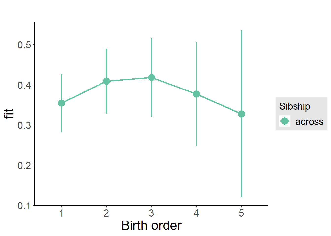
Add Interaction
Model Summary
m4_interaction = update(m3_birthorder_nonlinear, formula = . ~ . - birth_order_nonlinear - sibling_count + count_birth_order)
tidy(m4_interaction, conf.int = T, conf.level = 0.995)| effect | group | term | estimate | std.error | statistic | df | p.value | conf.low | conf.high |
|---|---|---|---|---|---|---|---|---|---|
| fixed | NA | (Intercept) | 0.08871 | 0.4612 | 0.1924 | 4473 | 0.8475 | -1.206 | 1.383 |
| fixed | NA | poly(age, 3, raw = TRUE)1 | 0.0111 | 0.0538 | 0.2063 | 4477 | 0.8366 | -0.1399 | 0.1621 |
| fixed | NA | poly(age, 3, raw = TRUE)2 | 0.0004685 | 0.001984 | 0.2361 | 4484 | 0.8134 | -0.005102 | 0.006039 |
| fixed | NA | poly(age, 3, raw = TRUE)3 | -0.00001987 | 0.00002327 | -0.8538 | 4490 | 0.3933 | -0.0000852 | 0.00004546 |
| fixed | NA | male | 0.07578 | 0.02461 | 3.079 | 4275 | 0.00209 | 0.006695 | 0.1449 |
| fixed | NA | count_birth_order2/2 | 0.0315 | 0.04953 | 0.636 | 3674 | 0.5248 | -0.1075 | 0.1705 |
| fixed | NA | count_birth_order1/3 | -0.01303 | 0.04503 | -0.2893 | 4466 | 0.7724 | -0.1394 | 0.1134 |
| fixed | NA | count_birth_order2/3 | 0.0853 | 0.04888 | 1.745 | 4501 | 0.08106 | -0.05192 | 0.2225 |
| fixed | NA | count_birth_order3/3 | 0.0798 | 0.05455 | 1.463 | 4493 | 0.1435 | -0.07332 | 0.2329 |
| fixed | NA | count_birth_order1/4 | -0.06294 | 0.05485 | -1.147 | 4497 | 0.2512 | -0.2169 | 0.09103 |
| fixed | NA | count_birth_order2/4 | -0.02508 | 0.05663 | -0.4429 | 4497 | 0.6578 | -0.184 | 0.1339 |
| fixed | NA | count_birth_order3/4 | 0.004614 | 0.05957 | 0.07745 | 4463 | 0.9383 | -0.1626 | 0.1718 |
| fixed | NA | count_birth_order4/4 | -0.01753 | 0.06194 | -0.283 | 4459 | 0.7772 | -0.1914 | 0.1563 |
| fixed | NA | count_birth_order1/5 | -0.0476 | 0.07444 | -0.6395 | 4484 | 0.5225 | -0.2565 | 0.1613 |
| fixed | NA | count_birth_order2/5 | -0.04182 | 0.07935 | -0.527 | 4399 | 0.5983 | -0.2646 | 0.1809 |
| fixed | NA | count_birth_order3/5 | -0.05883 | 0.07456 | -0.789 | 4408 | 0.4302 | -0.2681 | 0.1505 |
| fixed | NA | count_birth_order4/5 | -0.1101 | 0.072 | -1.529 | 4438 | 0.1262 | -0.3122 | 0.09199 |
| fixed | NA | count_birth_order5/5 | -0.128 | 0.07442 | -1.721 | 4410 | 0.08539 | -0.3369 | 0.08085 |
| ran_pars | mother_pidlink | sd__(Intercept) | 0.41 | NA | NA | NA | NA | NA | NA |
| ran_pars | Residual | sd__Observation | 0.7379 | NA | NA | NA | NA | NA | NA |
Coefficient Plot
plot_birthorder(m4_interaction)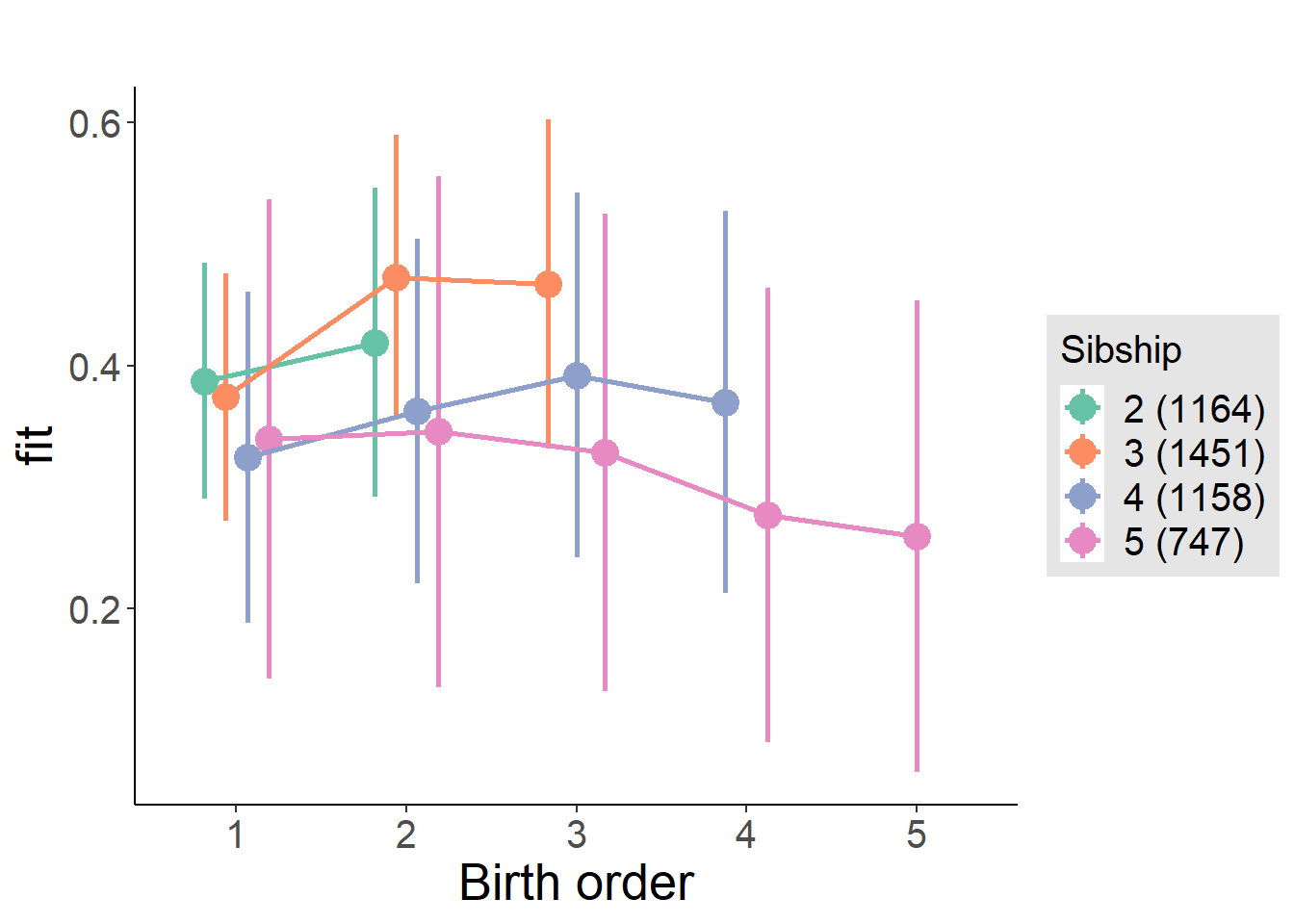
Model Comparison
###### Model 1 - Model 2
anova(m1_covariates_only, m2_birthorder_linear, m3_birthorder_nonlinear, m4_interaction)
## refitting model(s) with ML (instead of REML)| Df | AIC | BIC | logLik | deviance | Chisq | Chi Df | Pr(>Chisq) |
|---|---|---|---|---|---|---|---|
| 10 | 11211 | 11276 | -5596 | 11191 | NA | NA | NA |
| 11 | 11213 | 11283 | -5595 | 11191 | 0.8885 | 1 | 0.3459 |
| 14 | 11214 | 11304 | -5593 | 11186 | 4.8 | 3 | 0.187 |
| 20 | 11223 | 11352 | -5592 | 11183 | 2.476 | 6 | 0.8712 |
Maternal pregnancy order
outcome_preg_m1 <- update(m2_birthorder_linear, data = birthorder %>%
  mutate(sibling_count = sibling_count_uterus_preg_factor,
         birth_order_nonlinear = birthorder_uterus_preg_factor,
         birth_order = birthorder_uterus_preg,
         count_birth_order = count_birthorder_uterus_preg
         ) %>%
    filter(sibling_count != "1"))
compare_models_markdown(outcome_preg_m1)
Basic Model
Model Summary
m1_covariates_only <- update(m2_birthorder_linear, formula = . ~ . - birth_order)
tidy(m1_covariates_only, conf.int = T, conf.level = 0.995)| effect | group | term | estimate | std.error | statistic | df | p.value | conf.low | conf.high |
|---|---|---|---|---|---|---|---|---|---|
| fixed | NA | (Intercept) | 0.3212 | 0.4696 | 0.684 | 4155 | 0.494 | -0.9971 | 1.64 |
| fixed | NA | poly(age, 3, raw = TRUE)1 | -0.01712 | 0.0549 | -0.3118 | 4164 | 0.7552 | -0.1712 | 0.137 |
| fixed | NA | poly(age, 3, raw = TRUE)2 | 0.001505 | 0.002025 | 0.7428 | 4173 | 0.4576 | -0.004181 | 0.00719 |
| fixed | NA | poly(age, 3, raw = TRUE)3 | -0.0000321 | 0.00002375 | -1.351 | 4180 | 0.1766 | -0.00009877 | 0.00003457 |
| fixed | NA | male | 0.08135 | 0.02535 | 3.209 | 3990 | 0.001342 | 0.01019 | 0.1525 |
| fixed | NA | sibling_count3 | 0.03156 | 0.03734 | 0.8452 | 3051 | 0.3981 | -0.07325 | 0.1364 |
| fixed | NA | sibling_count4 | -0.01131 | 0.03961 | -0.2857 | 2793 | 0.7751 | -0.1225 | 0.09986 |
| fixed | NA | sibling_count5 | -0.01969 | 0.04263 | -0.4619 | 2555 | 0.6442 | -0.1394 | 0.09997 |
| ran_pars | mother_pidlink | sd__(Intercept) | 0.3934 | NA | NA | NA | NA | NA | NA |
| ran_pars | Residual | sd__Observation | 0.7378 | NA | NA | NA | NA | NA | NA |
Coefficient Plot
plot(allEffects(m1_covariates_only, confidence.level = 0.995))
Add Birth Order Linear
Model Summary
tidy(m2_birthorder_linear, conf.int = T, conf.level = 0.995)| effect | group | term | estimate | std.error | statistic | df | p.value | conf.low | conf.high |
|---|---|---|---|---|---|---|---|---|---|
| fixed | NA | (Intercept) | 0.304 | 0.4701 | 0.6466 | 4155 | 0.5179 | -1.016 | 1.624 |
| fixed | NA | birth_order | 0.01035 | 0.01277 | 0.8108 | 3824 | 0.4175 | -0.02549 | 0.0462 |
| fixed | NA | poly(age, 3, raw = TRUE)1 | -0.01666 | 0.0549 | -0.3035 | 4163 | 0.7615 | -0.1708 | 0.1374 |
| fixed | NA | poly(age, 3, raw = TRUE)2 | 0.00148 | 0.002026 | 0.7304 | 4171 | 0.4652 | -0.004207 | 0.007166 |
| fixed | NA | poly(age, 3, raw = TRUE)3 | -0.0000316 | 0.00002376 | -1.33 | 4178 | 0.1836 | -0.00009829 | 0.0000351 |
| fixed | NA | male | 0.08109 | 0.02535 | 3.198 | 3990 | 0.001393 | 0.009921 | 0.1523 |
| fixed | NA | sibling_count3 | 0.02674 | 0.0378 | 0.7074 | 3093 | 0.4794 | -0.07938 | 0.1329 |
| fixed | NA | sibling_count4 | -0.02204 | 0.04176 | -0.5277 | 2954 | 0.5977 | -0.1392 | 0.09517 |
| fixed | NA | sibling_count5 | -0.03686 | 0.0476 | -0.7744 | 2936 | 0.4387 | -0.1705 | 0.09674 |
| ran_pars | mother_pidlink | sd__(Intercept) | 0.393 | NA | NA | NA | NA | NA | NA |
| ran_pars | Residual | sd__Observation | 0.738 | NA | NA | NA | NA | NA | NA |
Coefficient Plot
plot_birthorder2(m2_birthorder_linear, separate = FALSE)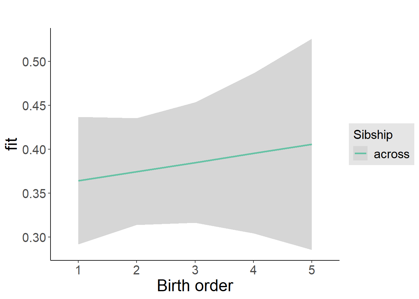
Add Birth Order Factor
Model Summary
m3_birthorder_nonlinear = update(m1_covariates_only, formula = . ~ . + birth_order_nonlinear)
tidy(m3_birthorder_nonlinear, conf.int = T, conf.level = 0.995)| effect | group | term | estimate | std.error | statistic | df | p.value | conf.low | conf.high |
|---|---|---|---|---|---|---|---|---|---|
| fixed | NA | (Intercept) | 0.2365 | 0.4707 | 0.5024 | 4164 | 0.6154 | -1.085 | 1.558 |
| fixed | NA | poly(age, 3, raw = TRUE)1 | -0.009492 | 0.05497 | -0.1727 | 4168 | 0.8629 | -0.1638 | 0.1448 |
| fixed | NA | poly(age, 3, raw = TRUE)2 | 0.00122 | 0.002028 | 0.6014 | 4174 | 0.5476 | -0.004473 | 0.006912 |
| fixed | NA | poly(age, 3, raw = TRUE)3 | -0.00002875 | 0.00002378 | -1.209 | 4179 | 0.2268 | -0.00009551 | 0.00003801 |
| fixed | NA | male | 0.08186 | 0.02535 | 3.23 | 3985 | 0.00125 | 0.01071 | 0.153 |
| fixed | NA | sibling_count3 | 0.0179 | 0.03829 | 0.4675 | 3190 | 0.6401 | -0.08957 | 0.1254 |
| fixed | NA | sibling_count4 | -0.02621 | 0.04227 | -0.62 | 3041 | 0.5353 | -0.1449 | 0.09245 |
| fixed | NA | sibling_count5 | -0.02217 | 0.04805 | -0.4613 | 2990 | 0.6446 | -0.157 | 0.1127 |
| fixed | NA | birth_order_nonlinear2 | 0.06266 | 0.0298 | 2.103 | 3193 | 0.03556 | -0.02099 | 0.1463 |
| fixed | NA | birth_order_nonlinear3 | 0.06276 | 0.03782 | 1.659 | 3399 | 0.09713 | -0.0434 | 0.1689 |
| fixed | NA | birth_order_nonlinear4 | 0.02567 | 0.0502 | 0.5113 | 3562 | 0.6092 | -0.1152 | 0.1666 |
| fixed | NA | birth_order_nonlinear5 | -0.03084 | 0.07318 | -0.4215 | 3413 | 0.6734 | -0.2363 | 0.1746 |
| ran_pars | mother_pidlink | sd__(Intercept) | 0.3932 | NA | NA | NA | NA | NA | NA |
| ran_pars | Residual | sd__Observation | 0.7376 | NA | NA | NA | NA | NA | NA |
Coefficient Plot
plot_birthorder(m3_birthorder_nonlinear, separate = FALSE)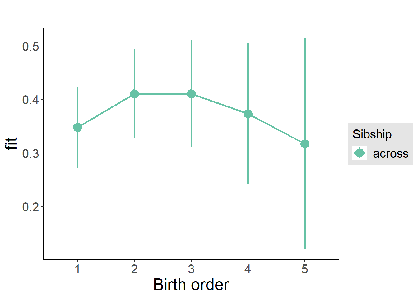
Add Interaction
Model Summary
m4_interaction = update(m3_birthorder_nonlinear, formula = . ~ . - birth_order_nonlinear - sibling_count + count_birth_order)
tidy(m4_interaction, conf.int = T, conf.level = 0.995)| effect | group | term | estimate | std.error | statistic | df | p.value | conf.low | conf.high |
|---|---|---|---|---|---|---|---|---|---|
| fixed | NA | (Intercept) | 0.267 | 0.4712 | 0.5668 | 4158 | 0.5709 | -1.056 | 1.59 |
| fixed | NA | poly(age, 3, raw = TRUE)1 | -0.01214 | 0.055 | -0.2208 | 4161 | 0.8253 | -0.1665 | 0.1422 |
| fixed | NA | poly(age, 3, raw = TRUE)2 | 0.001334 | 0.002029 | 0.6575 | 4168 | 0.5109 | -0.004362 | 0.007031 |
| fixed | NA | poly(age, 3, raw = TRUE)3 | -0.00003027 | 0.0000238 | -1.272 | 4173 | 0.2035 | -0.00009709 | 0.00003654 |
| fixed | NA | male | 0.08133 | 0.02537 | 3.206 | 3977 | 0.001356 | 0.01012 | 0.1525 |
| fixed | NA | count_birth_order2/2 | 0.02836 | 0.05401 | 0.5251 | 3462 | 0.5995 | -0.1232 | 0.18 |
| fixed | NA | count_birth_order1/3 | -0.005132 | 0.0483 | -0.1063 | 4152 | 0.9154 | -0.1407 | 0.1304 |
| fixed | NA | count_birth_order2/3 | 0.06901 | 0.05212 | 1.324 | 4180 | 0.1856 | -0.07729 | 0.2153 |
| fixed | NA | count_birth_order3/3 | 0.09276 | 0.0586 | 1.583 | 4172 | 0.1135 | -0.07172 | 0.2572 |
| fixed | NA | count_birth_order1/4 | -0.07718 | 0.05692 | -1.356 | 4175 | 0.1752 | -0.2369 | 0.08259 |
| fixed | NA | count_birth_order2/4 | 0.03891 | 0.05812 | 0.6695 | 4179 | 0.5032 | -0.1242 | 0.2021 |
| fixed | NA | count_birth_order3/4 | 0.0434 | 0.06328 | 0.6859 | 4140 | 0.4928 | -0.1342 | 0.221 |
| fixed | NA | count_birth_order4/4 | 0.01112 | 0.06527 | 0.1704 | 4144 | 0.8647 | -0.1721 | 0.1943 |
| fixed | NA | count_birth_order1/5 | 0.02681 | 0.06769 | 0.396 | 4180 | 0.6921 | -0.1632 | 0.2168 |
| fixed | NA | count_birth_order2/5 | 0.04688 | 0.07265 | 0.6452 | 4124 | 0.5188 | -0.1571 | 0.2508 |
| fixed | NA | count_birth_order3/5 | -0.03177 | 0.07038 | -0.4514 | 4119 | 0.6517 | -0.2293 | 0.1658 |
| fixed | NA | count_birth_order4/5 | -0.03833 | 0.0728 | -0.5265 | 4089 | 0.5986 | -0.2427 | 0.166 |
| fixed | NA | count_birth_order5/5 | -0.06641 | 0.07258 | -0.915 | 4097 | 0.3602 | -0.2701 | 0.1373 |
| ran_pars | mother_pidlink | sd__(Intercept) | 0.394 | NA | NA | NA | NA | NA | NA |
| ran_pars | Residual | sd__Observation | 0.7374 | NA | NA | NA | NA | NA | NA |
Coefficient Plot
plot_birthorder(m4_interaction)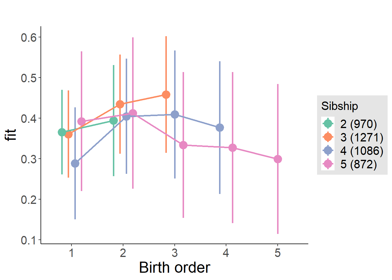
Model Comparison
###### Model 1 - Model 2
anova(m1_covariates_only, m2_birthorder_linear, m3_birthorder_nonlinear, m4_interaction)
## refitting model(s) with ML (instead of REML)| Df | AIC | BIC | logLik | deviance | Chisq | Chi Df | Pr(>Chisq) |
|---|---|---|---|---|---|---|---|
| 10 | 10350 | 10413 | -5165 | 10330 | NA | NA | NA |
| 11 | 10351 | 10421 | -5165 | 10329 | 0.6594 | 1 | 0.4168 |
| 14 | 10351 | 10440 | -5162 | 10323 | 5.737 | 3 | 0.1251 |
| 20 | 10359 | 10486 | -5159 | 10319 | 4.508 | 6 | 0.6083 |
Parental full sibling order
outcome_parental_m1 <- update(m2_birthorder_linear, data = birthorder %>%
  mutate(sibling_count = sibling_count_genes_factor,
         birth_order_nonlinear = birthorder_genes_factor,
         birth_order = birthorder_genes,
         count_birth_order = count_birthorder_genes
         ) %>%
      filter(sibling_count != "1"))
compare_models_markdown(outcome_parental_m1)
Basic Model
Model Summary
m1_covariates_only <- update(m2_birthorder_linear, formula = . ~ . - birth_order)
tidy(m1_covariates_only, conf.int = T, conf.level = 0.995)| effect | group | term | estimate | std.error | statistic | df | p.value | conf.low | conf.high |
|---|---|---|---|---|---|---|---|---|---|
| fixed | NA | (Intercept) | 0.1919 | 0.4629 | 0.4145 | 4454 | 0.6785 | -1.108 | 1.491 |
| fixed | NA | poly(age, 3, raw = TRUE)1 | 0.002144 | 0.05414 | 0.03959 | 4463 | 0.9684 | -0.1498 | 0.1541 |
| fixed | NA | poly(age, 3, raw = TRUE)2 | 0.0007434 | 0.002 | 0.3717 | 4472 | 0.7101 | -0.00487 | 0.006357 |
| fixed | NA | poly(age, 3, raw = TRUE)3 | -0.00002273 | 0.00002349 | -0.9674 | 4480 | 0.3334 | -0.00008867 | 0.00004322 |
| fixed | NA | male | 0.07125 | 0.02459 | 2.897 | 4279 | 0.003787 | 0.002212 | 0.1403 |
| fixed | NA | sibling_count3 | 0.02066 | 0.03446 | 0.5995 | 3229 | 0.5489 | -0.07606 | 0.1174 |
| fixed | NA | sibling_count4 | -0.03106 | 0.03762 | -0.8254 | 2914 | 0.4092 | -0.1367 | 0.07456 |
| fixed | NA | sibling_count5 | -0.0859 | 0.04475 | -1.92 | 2597 | 0.05502 | -0.2115 | 0.03972 |
| ran_pars | mother_pidlink | sd__(Intercept) | 0.4078 | NA | NA | NA | NA | NA | NA |
| ran_pars | Residual | sd__Observation | 0.7369 | NA | NA | NA | NA | NA | NA |
Coefficient Plot
plot(allEffects(m1_covariates_only, confidence.level = 0.995))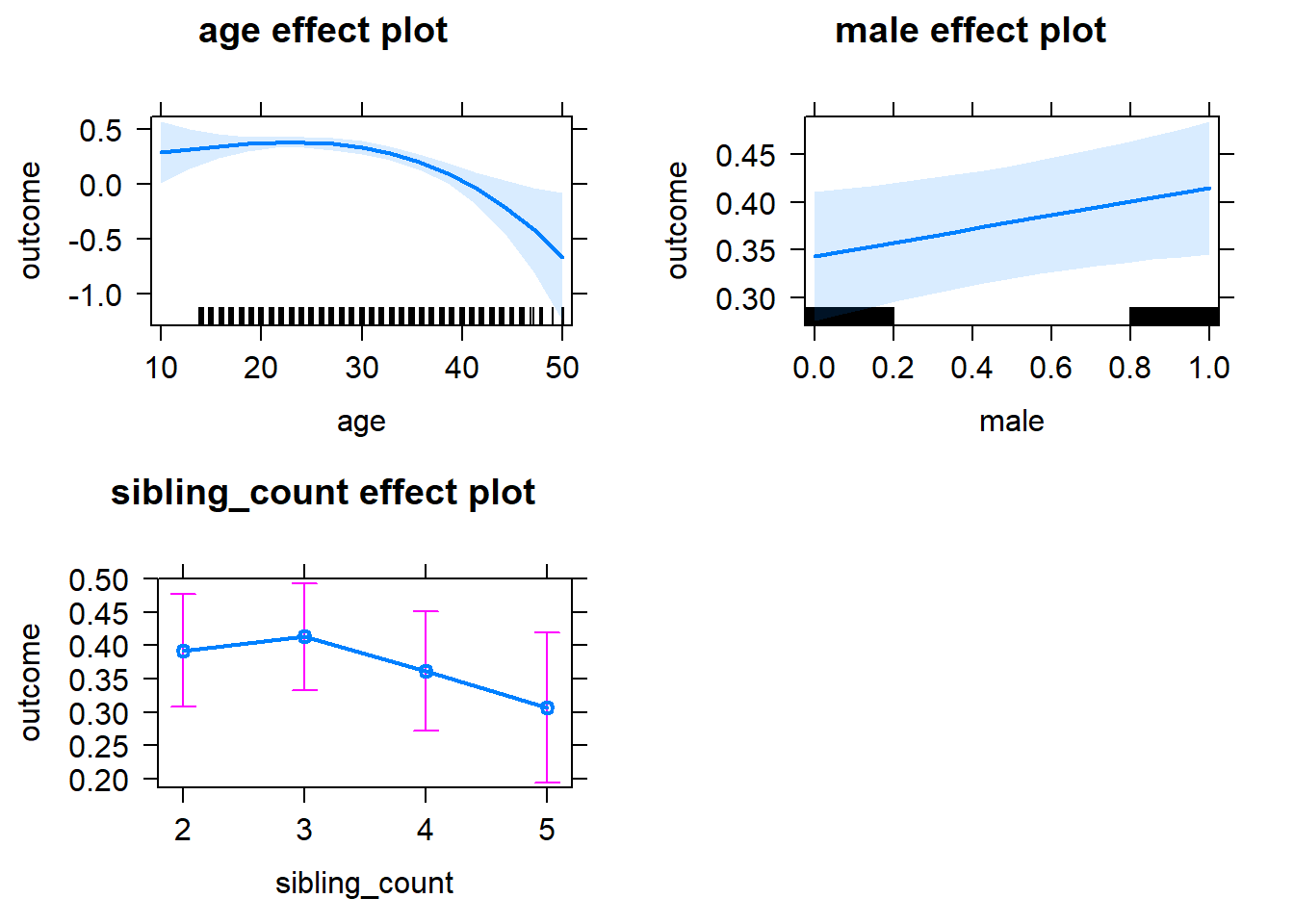
Add Birth Order Linear
Model Summary
tidy(m2_birthorder_linear, conf.int = T, conf.level = 0.995)| effect | group | term | estimate | std.error | statistic | df | p.value | conf.low | conf.high |
|---|---|---|---|---|---|---|---|---|---|
| fixed | NA | (Intercept) | 0.1688 | 0.4635 | 0.3643 | 4455 | 0.7157 | -1.132 | 1.47 |
| fixed | NA | birth_order | 0.01354 | 0.01294 | 1.046 | 3978 | 0.2955 | -0.02279 | 0.04987 |
| fixed | NA | poly(age, 3, raw = TRUE)1 | 0.002806 | 0.05415 | 0.05183 | 4462 | 0.9587 | -0.1492 | 0.1548 |
| fixed | NA | poly(age, 3, raw = TRUE)2 | 0.0007076 | 0.002 | 0.3538 | 4471 | 0.7235 | -0.004907 | 0.006322 |
| fixed | NA | poly(age, 3, raw = TRUE)3 | -0.00002203 | 0.0000235 | -0.9375 | 4478 | 0.3486 | -0.000088 | 0.00004394 |
| fixed | NA | male | 0.07082 | 0.0246 | 2.879 | 4277 | 0.004006 | 0.001777 | 0.1399 |
| fixed | NA | sibling_count3 | 0.01432 | 0.03499 | 0.4092 | 3282 | 0.6824 | -0.08389 | 0.1125 |
| fixed | NA | sibling_count4 | -0.0456 | 0.04011 | -1.137 | 3137 | 0.2557 | -0.1582 | 0.06699 |
| fixed | NA | sibling_count5 | -0.1092 | 0.04997 | -2.185 | 3031 | 0.02899 | -0.2494 | 0.0311 |
| ran_pars | mother_pidlink | sd__(Intercept) | 0.4079 | NA | NA | NA | NA | NA | NA |
| ran_pars | Residual | sd__Observation | 0.7369 | NA | NA | NA | NA | NA | NA |
Coefficient Plot
plot_birthorder2(m2_birthorder_linear, separate = FALSE)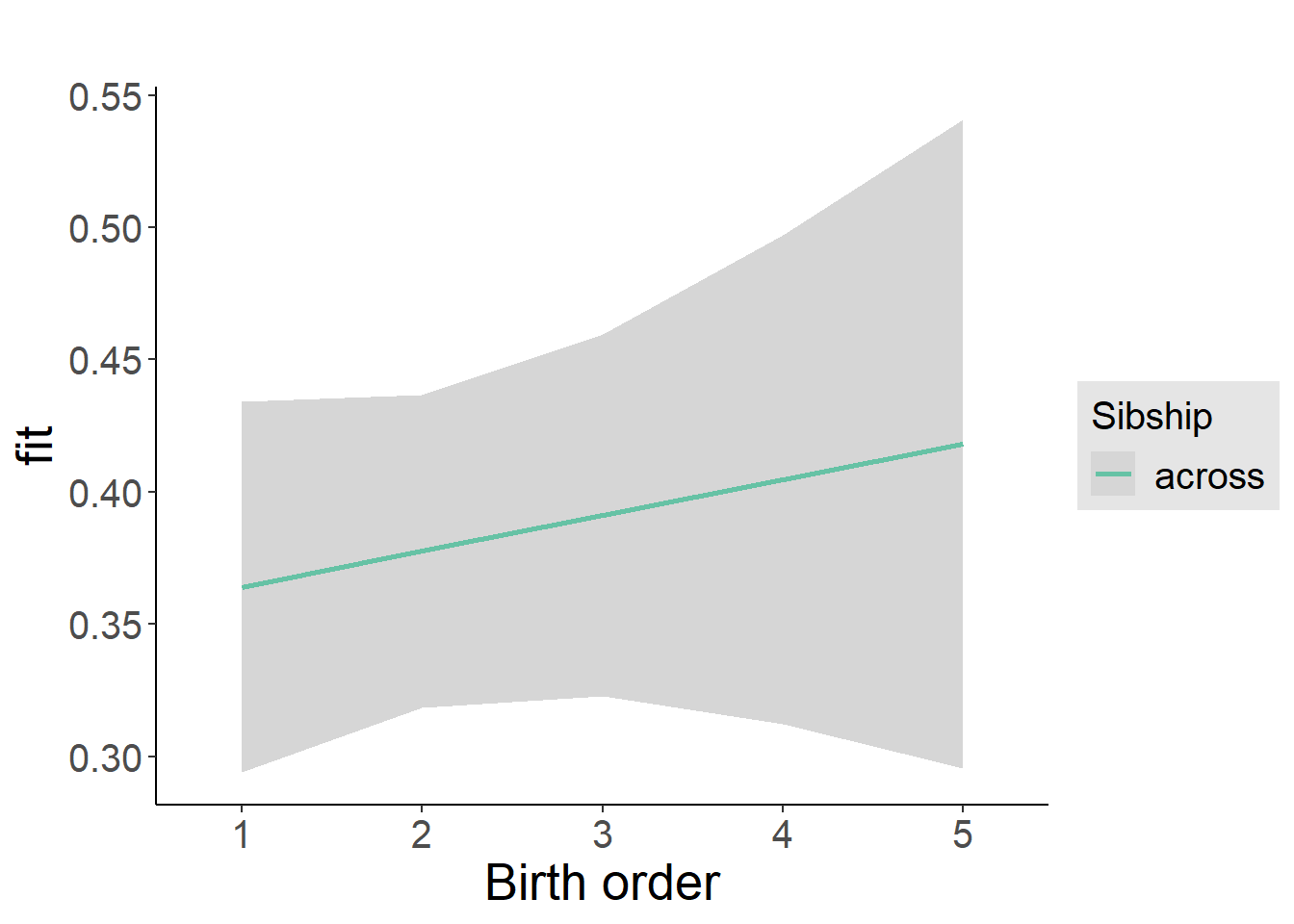
Add Birth Order Factor
Model Summary
m3_birthorder_nonlinear = update(m1_covariates_only, formula = . ~ . + birth_order_nonlinear)
tidy(m3_birthorder_nonlinear, conf.int = T, conf.level = 0.995)| effect | group | term | estimate | std.error | statistic | df | p.value | conf.low | conf.high |
|---|---|---|---|---|---|---|---|---|---|
| fixed | NA | (Intercept) | 0.09842 | 0.4641 | 0.2121 | 4464 | 0.8321 | -1.204 | 1.401 |
| fixed | NA | poly(age, 3, raw = TRUE)1 | 0.0104 | 0.05422 | 0.1918 | 4469 | 0.8479 | -0.1418 | 0.1626 |
| fixed | NA | poly(age, 3, raw = TRUE)2 | 0.0004386 | 0.002002 | 0.2191 | 4475 | 0.8266 | -0.005182 | 0.006059 |
| fixed | NA | poly(age, 3, raw = TRUE)3 | -0.00001915 | 0.00002352 | -0.8141 | 4480 | 0.4156 | -0.00008517 | 0.00004688 |
| fixed | NA | male | 0.07164 | 0.0246 | 2.913 | 4274 | 0.003602 | 0.002598 | 0.1407 |
| fixed | NA | sibling_count3 | 0.009576 | 0.03546 | 0.2701 | 3398 | 0.7871 | -0.08995 | 0.1091 |
| fixed | NA | sibling_count4 | -0.04664 | 0.04063 | -1.148 | 3234 | 0.2511 | -0.1607 | 0.0674 |
| fixed | NA | sibling_count5 | -0.08504 | 0.05087 | -1.672 | 3140 | 0.09465 | -0.2278 | 0.05774 |
| fixed | NA | birth_order_nonlinear2 | 0.06891 | 0.0285 | 2.417 | 3379 | 0.01568 | -0.0111 | 0.1489 |
| fixed | NA | birth_order_nonlinear3 | 0.05499 | 0.03656 | 1.504 | 3560 | 0.1326 | -0.04763 | 0.1576 |
| fixed | NA | birth_order_nonlinear4 | 0.03758 | 0.05054 | 0.7436 | 3747 | 0.4572 | -0.1043 | 0.1795 |
| fixed | NA | birth_order_nonlinear5 | -0.04573 | 0.08241 | -0.5549 | 3627 | 0.579 | -0.277 | 0.1856 |
| ran_pars | mother_pidlink | sd__(Intercept) | 0.4065 | NA | NA | NA | NA | NA | NA |
| ran_pars | Residual | sd__Observation | 0.7372 | NA | NA | NA | NA | NA | NA |
Coefficient Plot
plot_birthorder(m3_birthorder_nonlinear, separate = FALSE)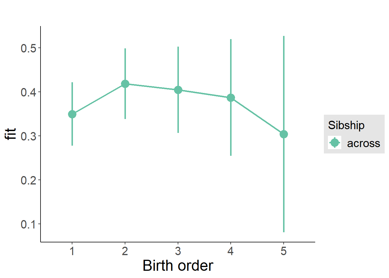
Add Interaction
Model Summary
m4_interaction = update(m3_birthorder_nonlinear, formula = . ~ . - birth_order_nonlinear - sibling_count + count_birth_order)
tidy(m4_interaction, conf.int = T, conf.level = 0.995)| effect | group | term | estimate | std.error | statistic | df | p.value | conf.low | conf.high |
|---|---|---|---|---|---|---|---|---|---|
| fixed | NA | (Intercept) | 0.1026 | 0.4645 | 0.2208 | 4458 | 0.8252 | -1.201 | 1.406 |
| fixed | NA | poly(age, 3, raw = TRUE)1 | 0.01011 | 0.05425 | 0.1864 | 4462 | 0.8521 | -0.1422 | 0.1624 |
| fixed | NA | poly(age, 3, raw = TRUE)2 | 0.0004652 | 0.002004 | 0.2322 | 4468 | 0.8164 | -0.00516 | 0.00609 |
| fixed | NA | poly(age, 3, raw = TRUE)3 | -0.00001964 | 0.00002354 | -0.834 | 4474 | 0.4043 | -0.00008572 | 0.00004645 |
| fixed | NA | male | 0.0719 | 0.02462 | 2.921 | 4268 | 0.003513 | 0.002794 | 0.141 |
| fixed | NA | count_birth_order2/2 | 0.05321 | 0.0481 | 1.106 | 3623 | 0.2686 | -0.08179 | 0.1882 |
| fixed | NA | count_birth_order1/3 | -0.01115 | 0.04436 | -0.2515 | 4451 | 0.8015 | -0.1357 | 0.1134 |
| fixed | NA | count_birth_order2/3 | 0.09775 | 0.04872 | 2.006 | 4486 | 0.0449 | -0.03902 | 0.2345 |
| fixed | NA | count_birth_order3/3 | 0.05654 | 0.05345 | 1.058 | 4473 | 0.2902 | -0.0935 | 0.2066 |
| fixed | NA | count_birth_order1/4 | -0.05762 | 0.05495 | -1.049 | 4484 | 0.2944 | -0.2119 | 0.09662 |
| fixed | NA | count_birth_order2/4 | -0.001019 | 0.05656 | -0.01801 | 4476 | 0.9856 | -0.1598 | 0.1578 |
| fixed | NA | count_birth_order3/4 | 0.01591 | 0.0589 | 0.2702 | 4445 | 0.787 | -0.1494 | 0.1812 |
| fixed | NA | count_birth_order4/4 | 0.002424 | 0.06205 | 0.03907 | 4428 | 0.9688 | -0.1717 | 0.1766 |
| fixed | NA | count_birth_order1/5 | -0.03924 | 0.07434 | -0.5279 | 4476 | 0.5976 | -0.2479 | 0.1694 |
| fixed | NA | count_birth_order2/5 | -0.03639 | 0.08185 | -0.4446 | 4374 | 0.6566 | -0.2662 | 0.1934 |
| fixed | NA | count_birth_order3/5 | -0.053 | 0.07775 | -0.6817 | 4384 | 0.4955 | -0.2712 | 0.1652 |
| fixed | NA | count_birth_order4/5 | -0.08061 | 0.07537 | -1.07 | 4413 | 0.2849 | -0.2922 | 0.1309 |
| fixed | NA | count_birth_order5/5 | -0.1373 | 0.07948 | -1.727 | 4383 | 0.0842 | -0.3604 | 0.08582 |
| ran_pars | mother_pidlink | sd__(Intercept) | 0.4056 | NA | NA | NA | NA | NA | NA |
| ran_pars | Residual | sd__Observation | 0.738 | NA | NA | NA | NA | NA | NA |
Coefficient Plot
plot_birthorder(m4_interaction)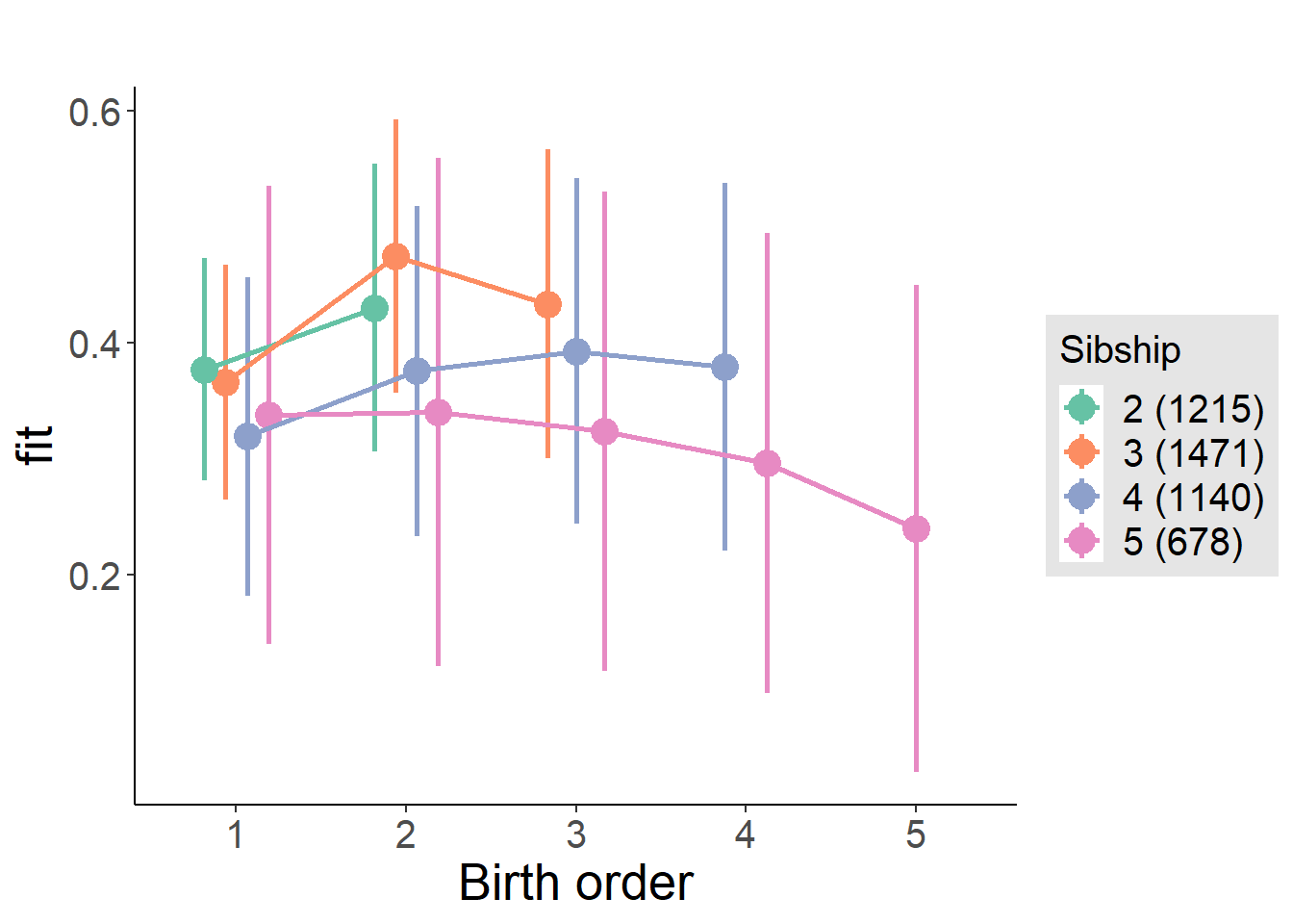
Model Comparison
###### Model 1 - Model 2
anova(m1_covariates_only, m2_birthorder_linear, m3_birthorder_nonlinear, m4_interaction)
## refitting model(s) with ML (instead of REML)| Df | AIC | BIC | logLik | deviance | Chisq | Chi Df | Pr(>Chisq) |
|---|---|---|---|---|---|---|---|
| 10 | 11153 | 11217 | -5567 | 11133 | NA | NA | NA |
| 11 | 11154 | 11225 | -5566 | 11132 | 1.096 | 1 | 0.2951 |
| 14 | 11154 | 11243 | -5563 | 11126 | 6.396 | 3 | 0.09386 |
| 20 | 11164 | 11292 | -5562 | 11124 | 2.068 | 6 | 0.9133 |
Compare birth order specifications
library(coefplot)
multiplot(outcome_naive_m1, outcome_preg_m1, outcome_uterus_m1, outcome_parental_m1, dodgeHeight = 0.6,
          intercept = FALSE)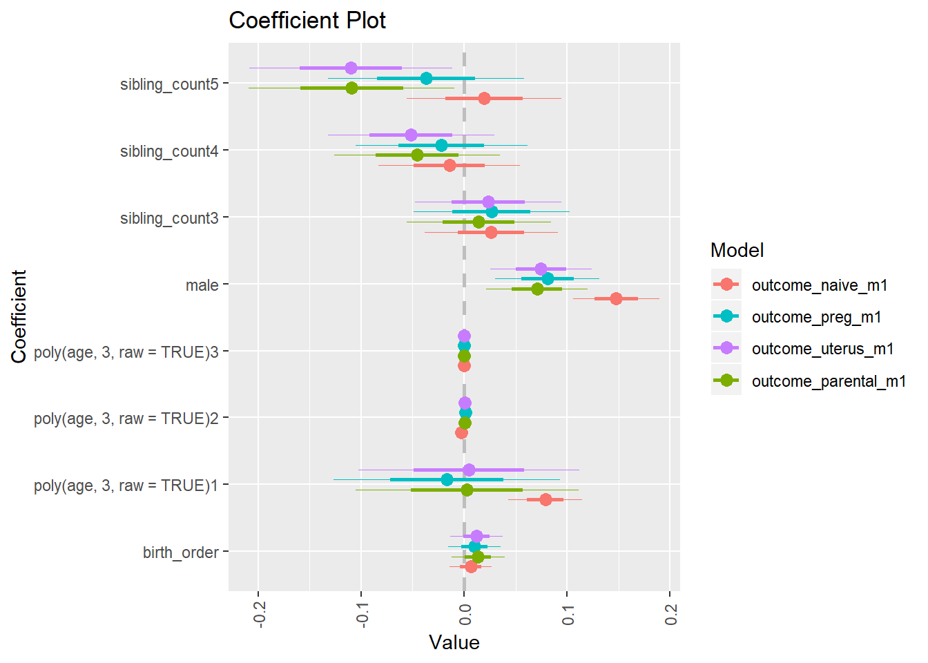
Numeracy 2015 old
birthorder <- birthorder %>% mutate(outcome = math_2015_old)
model = lmer(outcome ~ birth_order + poly(age, 3, raw = TRUE) + male + sibling_count + (1 | mother_pidlink),
                   data = birthorder)
compare_birthorder_specs(model)
Naive birth order
outcome_naive_m1 <- update(m2_birthorder_linear, data = birthorder %>%
                     mutate(sibling_count = sibling_count_naive_factor,
                            birth_order_nonlinear = birthorder_naive_factor,
                            birth_order = birthorder_naive,
                            count_birth_order = count_birthorder_naive) %>%
                     filter(sibling_count != "1"))
compare_models_markdown(outcome_naive_m1)
Basic Model
Model Summary
m1_covariates_only <- update(m2_birthorder_linear, formula = . ~ . - birth_order)
tidy(m1_covariates_only, conf.int = T, conf.level = 0.995)| effect | group | term | estimate | std.error | statistic | df | p.value | conf.low | conf.high |
|---|---|---|---|---|---|---|---|---|---|
| fixed | NA | (Intercept) | 0.1434 | 0.2829 | 0.507 | 7090 | 0.6121 | -0.6507 | 0.9376 |
| fixed | NA | poly(age, 3, raw = TRUE)1 | 0.03262 | 0.02914 | 1.119 | 7094 | 0.263 | -0.04919 | 0.1144 |
| fixed | NA | poly(age, 3, raw = TRUE)2 | -0.001464 | 0.000923 | -1.587 | 7093 | 0.1127 | -0.004055 | 0.001126 |
| fixed | NA | poly(age, 3, raw = TRUE)3 | 0.00001303 | 0.000009115 | 1.43 | 7085 | 0.1528 | -0.00001255 | 0.00003862 |
| fixed | NA | male | -0.1109 | 0.02366 | -4.687 | 6802 | 0.000002823 | -0.1773 | -0.04448 |
| fixed | NA | sibling_count3 | 0.02993 | 0.03547 | 0.8437 | 4996 | 0.3989 | -0.06964 | 0.1295 |
| fixed | NA | sibling_count4 | -0.05079 | 0.03669 | -1.384 | 4565 | 0.1663 | -0.1538 | 0.05219 |
| fixed | NA | sibling_count5 | -0.02016 | 0.0384 | -0.5251 | 4141 | 0.5995 | -0.128 | 0.08762 |
| ran_pars | mother_pidlink | sd__(Intercept) | 0.4687 | NA | NA | NA | NA | NA | NA |
| ran_pars | Residual | sd__Observation | 0.9013 | NA | NA | NA | NA | NA | NA |
Coefficient Plot
plot(allEffects(m1_covariates_only, confidence.level = 0.995))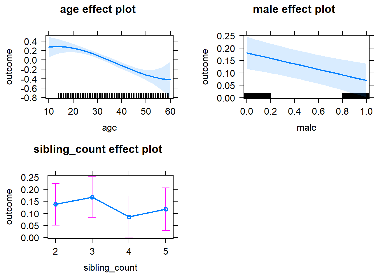
Add Birth Order Linear
Model Summary
tidy(m2_birthorder_linear, conf.int = T, conf.level = 0.995)| effect | group | term | estimate | std.error | statistic | df | p.value | conf.low | conf.high |
|---|---|---|---|---|---|---|---|---|---|
| fixed | NA | (Intercept) | 0.1297 | 0.2833 | 0.4579 | 7093 | 0.647 | -0.6656 | 0.9251 |
| fixed | NA | birth_order | 0.01012 | 0.01162 | 0.8706 | 5810 | 0.384 | -0.0225 | 0.04273 |
| fixed | NA | poly(age, 3, raw = TRUE)1 | 0.03262 | 0.02914 | 1.119 | 7093 | 0.2631 | -0.04919 | 0.1144 |
| fixed | NA | poly(age, 3, raw = TRUE)2 | -0.001471 | 0.0009231 | -1.593 | 7092 | 0.1111 | -0.004062 | 0.00112 |
| fixed | NA | poly(age, 3, raw = TRUE)3 | 0.0000132 | 0.000009117 | 1.448 | 7084 | 0.1478 | -0.00001239 | 0.00003879 |
| fixed | NA | male | -0.1111 | 0.02366 | -4.697 | 6801 | 0.000002695 | -0.1775 | -0.04471 |
| fixed | NA | sibling_count3 | 0.02648 | 0.03569 | 0.7421 | 5107 | 0.4581 | -0.07369 | 0.1267 |
| fixed | NA | sibling_count4 | -0.05896 | 0.03787 | -1.557 | 5033 | 0.1195 | -0.1653 | 0.04733 |
| fixed | NA | sibling_count5 | -0.03345 | 0.04132 | -0.8096 | 5084 | 0.4182 | -0.1495 | 0.08254 |
| ran_pars | mother_pidlink | sd__(Intercept) | 0.4683 | NA | NA | NA | NA | NA | NA |
| ran_pars | Residual | sd__Observation | 0.9016 | NA | NA | NA | NA | NA | NA |
Coefficient Plot
plot_birthorder2(m2_birthorder_linear, separate = FALSE)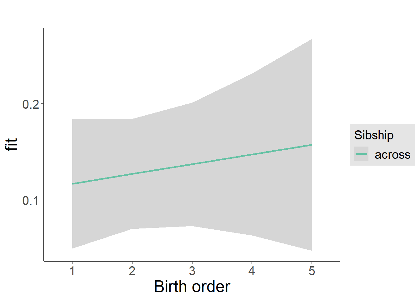
Add Birth Order Factor
Model Summary
m3_birthorder_nonlinear = update(m1_covariates_only, formula = . ~ . + birth_order_nonlinear)
tidy(m3_birthorder_nonlinear, conf.int = T, conf.level = 0.995)| effect | group | term | estimate | std.error | statistic | df | p.value | conf.low | conf.high |
|---|---|---|---|---|---|---|---|---|---|
| fixed | NA | (Intercept) | 0.1785 | 0.2849 | 0.6265 | 7095 | 0.531 | -0.6213 | 0.9784 |
| fixed | NA | poly(age, 3, raw = TRUE)1 | 0.02929 | 0.02929 | 0.9999 | 7096 | 0.3174 | -0.05293 | 0.1115 |
| fixed | NA | poly(age, 3, raw = TRUE)2 | -0.001352 | 0.0009288 | -1.456 | 7097 | 0.1456 | -0.003959 | 0.001255 |
| fixed | NA | poly(age, 3, raw = TRUE)3 | 0.00001193 | 0.000009182 | 1.299 | 7095 | 0.1941 | -0.00001385 | 0.0000377 |
| fixed | NA | male | -0.1111 | 0.02366 | -4.696 | 6798 | 0.000002711 | -0.1775 | -0.04469 |
| fixed | NA | sibling_count3 | 0.02668 | 0.03616 | 0.7376 | 5291 | 0.4608 | -0.07484 | 0.1282 |
| fixed | NA | sibling_count4 | -0.05799 | 0.03839 | -1.511 | 5238 | 0.131 | -0.1658 | 0.04977 |
| fixed | NA | sibling_count5 | -0.04003 | 0.04162 | -0.9616 | 5229 | 0.3363 | -0.1569 | 0.07681 |
| fixed | NA | birth_order_nonlinear2 | -0.01975 | 0.02777 | -0.7111 | 5850 | 0.4771 | -0.0977 | 0.05821 |
| fixed | NA | birth_order_nonlinear3 | 0.01226 | 0.03543 | 0.3459 | 5621 | 0.7294 | -0.08721 | 0.1117 |
| fixed | NA | birth_order_nonlinear4 | 0.01825 | 0.04599 | 0.3969 | 5528 | 0.6915 | -0.1108 | 0.1474 |
| fixed | NA | birth_order_nonlinear5 | 0.07661 | 0.06708 | 1.142 | 5305 | 0.2535 | -0.1117 | 0.2649 |
| ran_pars | mother_pidlink | sd__(Intercept) | 0.4678 | NA | NA | NA | NA | NA | NA |
| ran_pars | Residual | sd__Observation | 0.9019 | NA | NA | NA | NA | NA | NA |
Coefficient Plot
plot_birthorder(m3_birthorder_nonlinear, separate = FALSE)
Add Interaction
Model Summary
m4_interaction = update(m3_birthorder_nonlinear, formula = . ~ . - birth_order_nonlinear - sibling_count + count_birth_order)
tidy(m4_interaction, conf.int = T, conf.level = 0.995)| effect | group | term | estimate | std.error | statistic | df | p.value | conf.low | conf.high |
|---|---|---|---|---|---|---|---|---|---|
| fixed | NA | (Intercept) | 0.1745 | 0.2856 | 0.6108 | 7090 | 0.5413 | -0.6273 | 0.9762 |
| fixed | NA | poly(age, 3, raw = TRUE)1 | 0.02899 | 0.02931 | 0.989 | 7091 | 0.3227 | -0.05329 | 0.1113 |
| fixed | NA | poly(age, 3, raw = TRUE)2 | -0.001338 | 0.0009298 | -1.44 | 7091 | 0.15 | -0.003948 | 0.001271 |
| fixed | NA | poly(age, 3, raw = TRUE)3 | 0.00001176 | 0.000009195 | 1.279 | 7090 | 0.201 | -0.00001405 | 0.00003757 |
| fixed | NA | male | -0.1106 | 0.02367 | -4.671 | 6790 | 0.000003055 | -0.177 | -0.04413 |
| fixed | NA | count_birth_order2/2 | -0.004851 | 0.04751 | -0.1021 | 5942 | 0.9187 | -0.1382 | 0.1285 |
| fixed | NA | count_birth_order1/3 | 0.04678 | 0.04599 | 1.017 | 7020 | 0.3091 | -0.08232 | 0.1759 |
| fixed | NA | count_birth_order2/3 | 0.009359 | 0.05116 | 0.1829 | 7076 | 0.8548 | -0.1342 | 0.153 |
| fixed | NA | count_birth_order3/3 | 0.01759 | 0.05729 | 0.307 | 7088 | 0.7588 | -0.1432 | 0.1784 |
| fixed | NA | count_birth_order1/4 | -0.05097 | 0.05213 | -0.9777 | 7078 | 0.3283 | -0.1973 | 0.09537 |
| fixed | NA | count_birth_order2/4 | -0.06209 | 0.05497 | -1.13 | 7090 | 0.2587 | -0.2164 | 0.09221 |
| fixed | NA | count_birth_order3/4 | -0.03653 | 0.05945 | -0.6145 | 7080 | 0.5389 | -0.2034 | 0.1303 |
| fixed | NA | count_birth_order4/4 | -0.05719 | 0.06261 | -0.9135 | 7061 | 0.361 | -0.233 | 0.1186 |
| fixed | NA | count_birth_order1/5 | -0.05291 | 0.05914 | -0.8945 | 7089 | 0.3711 | -0.2189 | 0.1131 |
| fixed | NA | count_birth_order2/5 | -0.08266 | 0.06194 | -1.334 | 7075 | 0.1821 | -0.2565 | 0.09121 |
| fixed | NA | count_birth_order3/5 | 0.007637 | 0.06371 | 0.1199 | 7056 | 0.9046 | -0.1712 | 0.1865 |
| fixed | NA | count_birth_order4/5 | 0.01128 | 0.06732 | 0.1675 | 7019 | 0.8669 | -0.1777 | 0.2003 |
| fixed | NA | count_birth_order5/5 | 0.04267 | 0.06897 | 0.6187 | 6998 | 0.5361 | -0.1509 | 0.2363 |
| ran_pars | mother_pidlink | sd__(Intercept) | 0.4682 | NA | NA | NA | NA | NA | NA |
| ran_pars | Residual | sd__Observation | 0.902 | NA | NA | NA | NA | NA | NA |
Coefficient Plot
plot_birthorder(m4_interaction)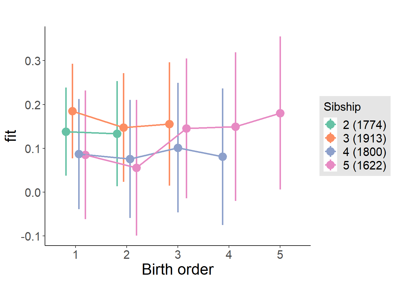
Model Comparison
###### Model 1 - Model 2
anova(m1_covariates_only, m2_birthorder_linear, m3_birthorder_nonlinear, m4_interaction)
## refitting model(s) with ML (instead of REML)| Df | AIC | BIC | logLik | deviance | Chisq | Chi Df | Pr(>Chisq) |
|---|---|---|---|---|---|---|---|
| 10 | 20269 | 20338 | -10125 | 20249 | NA | NA | NA |
| 11 | 20271 | 20346 | -10124 | 20249 | 0.7595 | 1 | 0.3835 |
| 14 | 20275 | 20371 | -10123 | 20247 | 1.755 | 3 | 0.6249 |
| 20 | 20285 | 20422 | -10123 | 20245 | 1.911 | 6 | 0.9277 |
Maternal birth order
outcome_uterus_m1 <- update(m2_birthorder_linear, data = birthorder %>%
                     mutate(sibling_count = sibling_count_uterus_alive_factor,
                            birth_order_nonlinear = birthorder_uterus_alive_factor,
                            birth_order = birthorder_uterus_alive,
                            count_birth_order = count_birthorder_uterus_alive) %>%
                     filter(sibling_count != "1"))
compare_models_markdown(outcome_uterus_m1)
Basic Model
Model Summary
m1_covariates_only <- update(m2_birthorder_linear, formula = . ~ . - birth_order)
tidy(m1_covariates_only, conf.int = T, conf.level = 0.995)| effect | group | term | estimate | std.error | statistic | df | p.value | conf.low | conf.high |
|---|---|---|---|---|---|---|---|---|---|
| fixed | NA | (Intercept) | -0.245 | 0.5633 | -0.4349 | 4496 | 0.6636 | -1.826 | 1.336 |
| fixed | NA | poly(age, 3, raw = TRUE)1 | 0.07656 | 0.06578 | 1.164 | 4502 | 0.2445 | -0.1081 | 0.2612 |
| fixed | NA | poly(age, 3, raw = TRUE)2 | -0.002516 | 0.002426 | -1.037 | 4507 | 0.2997 | -0.009324 | 0.004293 |
| fixed | NA | poly(age, 3, raw = TRUE)3 | 0.00002232 | 0.00002843 | 0.785 | 4510 | 0.4325 | -0.00005749 | 0.0001021 |
| fixed | NA | male | -0.18 | 0.03021 | -5.959 | 4381 | 0.000000002737 | -0.2649 | -0.09523 |
| fixed | NA | sibling_count3 | 0.01108 | 0.04228 | 0.2621 | 3364 | 0.7932 | -0.1076 | 0.1298 |
| fixed | NA | sibling_count4 | -0.0854 | 0.04575 | -1.867 | 3018 | 0.06205 | -0.2138 | 0.04302 |
| fixed | NA | sibling_count5 | -0.1326 | 0.05257 | -2.523 | 2748 | 0.01169 | -0.2802 | 0.01493 |
| ran_pars | mother_pidlink | sd__(Intercept) | 0.4446 | NA | NA | NA | NA | NA | NA |
| ran_pars | Residual | sd__Observation | 0.9278 | NA | NA | NA | NA | NA | NA |
Coefficient Plot
plot(allEffects(m1_covariates_only, confidence.level = 0.995))
Add Birth Order Linear
Model Summary
tidy(m2_birthorder_linear, conf.int = T, conf.level = 0.995)| effect | group | term | estimate | std.error | statistic | df | p.value | conf.low | conf.high |
|---|---|---|---|---|---|---|---|---|---|
| fixed | NA | (Intercept) | -0.2722 | 0.5639 | -0.4826 | 4496 | 0.6294 | -1.855 | 1.311 |
| fixed | NA | birth_order | 0.01604 | 0.01578 | 1.017 | 4123 | 0.3093 | -0.02824 | 0.06033 |
| fixed | NA | poly(age, 3, raw = TRUE)1 | 0.07742 | 0.06578 | 1.177 | 4501 | 0.2393 | -0.1072 | 0.2621 |
| fixed | NA | poly(age, 3, raw = TRUE)2 | -0.002563 | 0.002426 | -1.056 | 4506 | 0.2909 | -0.009372 | 0.004247 |
| fixed | NA | poly(age, 3, raw = TRUE)3 | 0.0000232 | 0.00002845 | 0.8156 | 4509 | 0.4148 | -0.00005665 | 0.000103 |
| fixed | NA | male | -0.1807 | 0.03022 | -5.979 | 4380 | 0.000000002426 | -0.2655 | -0.09585 |
| fixed | NA | sibling_count3 | 0.003624 | 0.04291 | 0.08448 | 3421 | 0.9327 | -0.1168 | 0.1241 |
| fixed | NA | sibling_count4 | -0.1025 | 0.04875 | -2.103 | 3229 | 0.03554 | -0.2394 | 0.03432 |
| fixed | NA | sibling_count5 | -0.1612 | 0.05961 | -2.705 | 3234 | 0.006873 | -0.3286 | 0.006103 |
| ran_pars | mother_pidlink | sd__(Intercept) | 0.4442 | NA | NA | NA | NA | NA | NA |
| ran_pars | Residual | sd__Observation | 0.928 | NA | NA | NA | NA | NA | NA |
Coefficient Plot
plot_birthorder2(m2_birthorder_linear, separate = FALSE)
Add Birth Order Factor
Model Summary
m3_birthorder_nonlinear = update(m1_covariates_only, formula = . ~ . + birth_order_nonlinear)
tidy(m3_birthorder_nonlinear, conf.int = T, conf.level = 0.995)| effect | group | term | estimate | std.error | statistic | df | p.value | conf.low | conf.high |
|---|---|---|---|---|---|---|---|---|---|
| fixed | NA | (Intercept) | -0.2693 | 0.5649 | -0.4766 | 4499 | 0.6337 | -1.855 | 1.317 |
| fixed | NA | poly(age, 3, raw = TRUE)1 | 0.07898 | 0.0659 | 1.199 | 4502 | 0.2307 | -0.106 | 0.264 |
| fixed | NA | poly(age, 3, raw = TRUE)2 | -0.002617 | 0.00243 | -1.077 | 4505 | 0.2816 | -0.009438 | 0.004204 |
| fixed | NA | poly(age, 3, raw = TRUE)3 | 0.00002375 | 0.00002849 | 0.8338 | 4507 | 0.4045 | -0.00005621 | 0.0001037 |
| fixed | NA | male | -0.1804 | 0.03024 | -5.965 | 4377 | 0.000000002633 | -0.2652 | -0.09549 |
| fixed | NA | sibling_count3 | -0.003152 | 0.04353 | -0.07241 | 3528 | 0.9423 | -0.1253 | 0.119 |
| fixed | NA | sibling_count4 | -0.1027 | 0.04943 | -2.078 | 3321 | 0.0378 | -0.2415 | 0.03605 |
| fixed | NA | sibling_count5 | -0.1596 | 0.06058 | -2.635 | 3325 | 0.008445 | -0.3297 | 0.0104 |
| fixed | NA | birth_order_nonlinear2 | 0.01484 | 0.03555 | 0.4174 | 3574 | 0.6764 | -0.08496 | 0.1146 |
| fixed | NA | birth_order_nonlinear3 | 0.06235 | 0.04546 | 1.372 | 3772 | 0.1702 | -0.06525 | 0.19 |
| fixed | NA | birth_order_nonlinear4 | 0.01672 | 0.06126 | 0.2729 | 3946 | 0.785 | -0.1552 | 0.1887 |
| fixed | NA | birth_order_nonlinear5 | 0.06174 | 0.09519 | 0.6486 | 3779 | 0.5167 | -0.2055 | 0.329 |
| ran_pars | mother_pidlink | sd__(Intercept) | 0.4437 | NA | NA | NA | NA | NA | NA |
| ran_pars | Residual | sd__Observation | 0.9284 | NA | NA | NA | NA | NA | NA |
Coefficient Plot
plot_birthorder(m3_birthorder_nonlinear, separate = FALSE)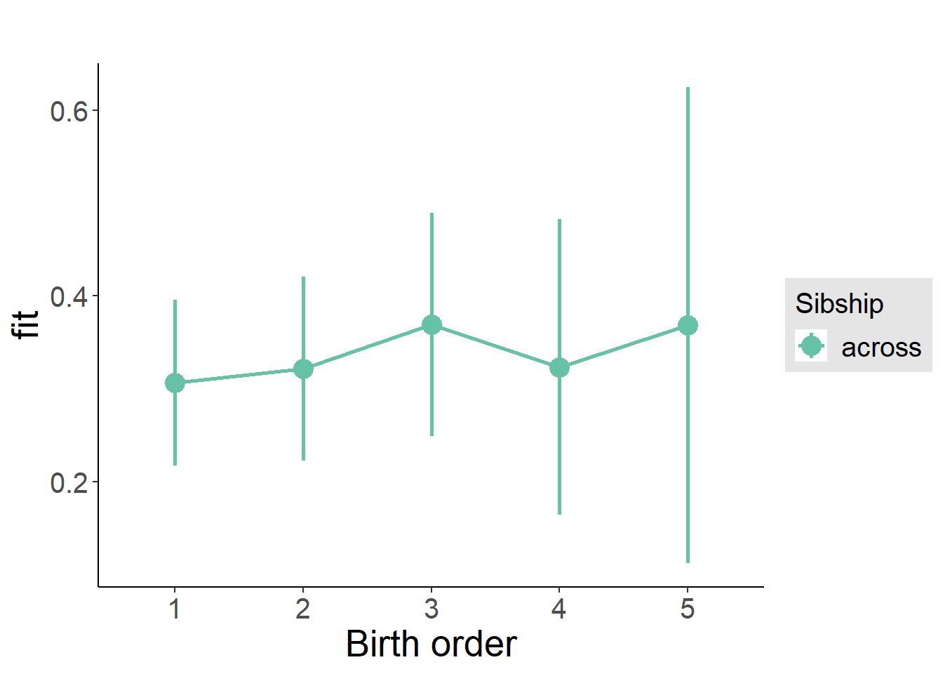
Add Interaction
Model Summary
m4_interaction = update(m3_birthorder_nonlinear, formula = . ~ . - birth_order_nonlinear - sibling_count + count_birth_order)
tidy(m4_interaction, conf.int = T, conf.level = 0.995)| effect | group | term | estimate | std.error | statistic | df | p.value | conf.low | conf.high |
|---|---|---|---|---|---|---|---|---|---|
| fixed | NA | (Intercept) | -0.2688 | 0.5653 | -0.4755 | 4493 | 0.6345 | -1.856 | 1.318 |
| fixed | NA | poly(age, 3, raw = TRUE)1 | 0.07764 | 0.06593 | 1.178 | 4496 | 0.239 | -0.1074 | 0.2627 |
| fixed | NA | poly(age, 3, raw = TRUE)2 | -0.002554 | 0.002431 | -1.051 | 4499 | 0.2935 | -0.00938 | 0.004271 |
| fixed | NA | poly(age, 3, raw = TRUE)3 | 0.00002289 | 0.00002851 | 0.8031 | 4501 | 0.422 | -0.00005713 | 0.0001029 |
| fixed | NA | male | -0.1798 | 0.03026 | -5.941 | 4370 | 0.000000003045 | -0.2647 | -0.09485 |
| fixed | NA | count_birth_order2/2 | 0.03824 | 0.06123 | 0.6246 | 3805 | 0.5322 | -0.1336 | 0.2101 |
| fixed | NA | count_birth_order1/3 | 0.006112 | 0.05503 | 0.1111 | 4482 | 0.9116 | -0.1483 | 0.1606 |
| fixed | NA | count_birth_order2/3 | 0.02754 | 0.05983 | 0.4604 | 4501 | 0.6452 | -0.1404 | 0.1955 |
| fixed | NA | count_birth_order3/3 | 0.05204 | 0.06684 | 0.7787 | 4495 | 0.4362 | -0.1356 | 0.2397 |
| fixed | NA | count_birth_order1/4 | -0.09395 | 0.0671 | -1.4 | 4498 | 0.1615 | -0.2823 | 0.0944 |
| fixed | NA | count_birth_order2/4 | -0.1263 | 0.06936 | -1.82 | 4499 | 0.06876 | -0.321 | 0.06843 |
| fixed | NA | count_birth_order3/4 | -0.03124 | 0.07305 | -0.4277 | 4476 | 0.6689 | -0.2363 | 0.1738 |
| fixed | NA | count_birth_order4/4 | -0.02205 | 0.07596 | -0.2902 | 4474 | 0.7717 | -0.2353 | 0.1912 |
| fixed | NA | count_birth_order1/5 | -0.1231 | 0.09123 | -1.349 | 4492 | 0.1774 | -0.3792 | 0.133 |
| fixed | NA | count_birth_order2/5 | -0.1036 | 0.09742 | -1.063 | 4441 | 0.2876 | -0.3771 | 0.1699 |
| fixed | NA | count_birth_order3/5 | -0.05967 | 0.09153 | -0.652 | 4444 | 0.5145 | -0.3166 | 0.1973 |
| fixed | NA | count_birth_order4/5 | -0.2167 | 0.08834 | -2.453 | 4460 | 0.0142 | -0.4647 | 0.03127 |
| fixed | NA | count_birth_order5/5 | -0.09149 | 0.09136 | -1.001 | 4441 | 0.3166 | -0.3479 | 0.165 |
| ran_pars | mother_pidlink | sd__(Intercept) | 0.4432 | NA | NA | NA | NA | NA | NA |
| ran_pars | Residual | sd__Observation | 0.929 | NA | NA | NA | NA | NA | NA |
Coefficient Plot
plot_birthorder(m4_interaction)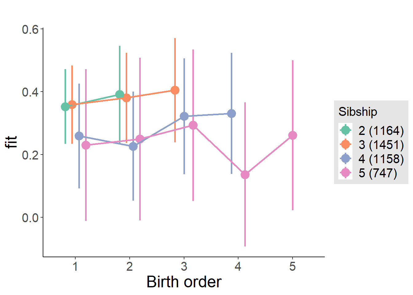
Model Comparison
###### Model 1 - Model 2
anova(m1_covariates_only, m2_birthorder_linear, m3_birthorder_nonlinear, m4_interaction)
## refitting model(s) with ML (instead of REML)| Df | AIC | BIC | logLik | deviance | Chisq | Chi Df | Pr(>Chisq) |
|---|---|---|---|---|---|---|---|
| 10 | 13037 | 13101 | -6509 | 13017 | NA | NA | NA |
| 11 | 13038 | 13109 | -6508 | 13016 | 1.037 | 1 | 0.3086 |
| 14 | 13043 | 13133 | -6507 | 13015 | 1.053 | 3 | 0.7884 |
| 20 | 13052 | 13180 | -6506 | 13012 | 3.242 | 6 | 0.778 |
Maternal pregnancy order
outcome_preg_m1 <- update(m2_birthorder_linear, data = birthorder %>%
  mutate(sibling_count = sibling_count_uterus_preg_factor,
         birth_order_nonlinear = birthorder_uterus_preg_factor,
         birth_order = birthorder_uterus_preg,
         count_birth_order = count_birthorder_uterus_preg
         ) %>%
    filter(sibling_count != "1"))
compare_models_markdown(outcome_preg_m1)
Basic Model
Model Summary
m1_covariates_only <- update(m2_birthorder_linear, formula = . ~ . - birth_order)
tidy(m1_covariates_only, conf.int = T, conf.level = 0.995)| effect | group | term | estimate | std.error | statistic | df | p.value | conf.low | conf.high |
|---|---|---|---|---|---|---|---|---|---|
| fixed | NA | (Intercept) | -0.3124 | 0.5809 | -0.5378 | 4175 | 0.5907 | -1.943 | 1.318 |
| fixed | NA | poly(age, 3, raw = TRUE)1 | 0.08482 | 0.06788 | 1.25 | 4181 | 0.2115 | -0.1057 | 0.2754 |
| fixed | NA | poly(age, 3, raw = TRUE)2 | -0.002853 | 0.002504 | -1.139 | 4186 | 0.2546 | -0.009882 | 0.004176 |
| fixed | NA | poly(age, 3, raw = TRUE)3 | 0.00002625 | 0.00002936 | 0.8941 | 4189 | 0.3713 | -0.00005616 | 0.0001087 |
| fixed | NA | male | -0.1795 | 0.03141 | -5.716 | 4065 | 0.00000001172 | -0.2677 | -0.09135 |
| fixed | NA | sibling_count3 | 0.02764 | 0.04572 | 0.6045 | 3205 | 0.5455 | -0.1007 | 0.156 |
| fixed | NA | sibling_count4 | -0.07076 | 0.04843 | -1.461 | 2948 | 0.1441 | -0.2067 | 0.06519 |
| fixed | NA | sibling_count5 | -0.08049 | 0.05206 | -1.546 | 2701 | 0.1222 | -0.2266 | 0.06564 |
| ran_pars | mother_pidlink | sd__(Intercept) | 0.4434 | NA | NA | NA | NA | NA | NA |
| ran_pars | Residual | sd__Observation | 0.9298 | NA | NA | NA | NA | NA | NA |
Coefficient Plot
plot(allEffects(m1_covariates_only, confidence.level = 0.995))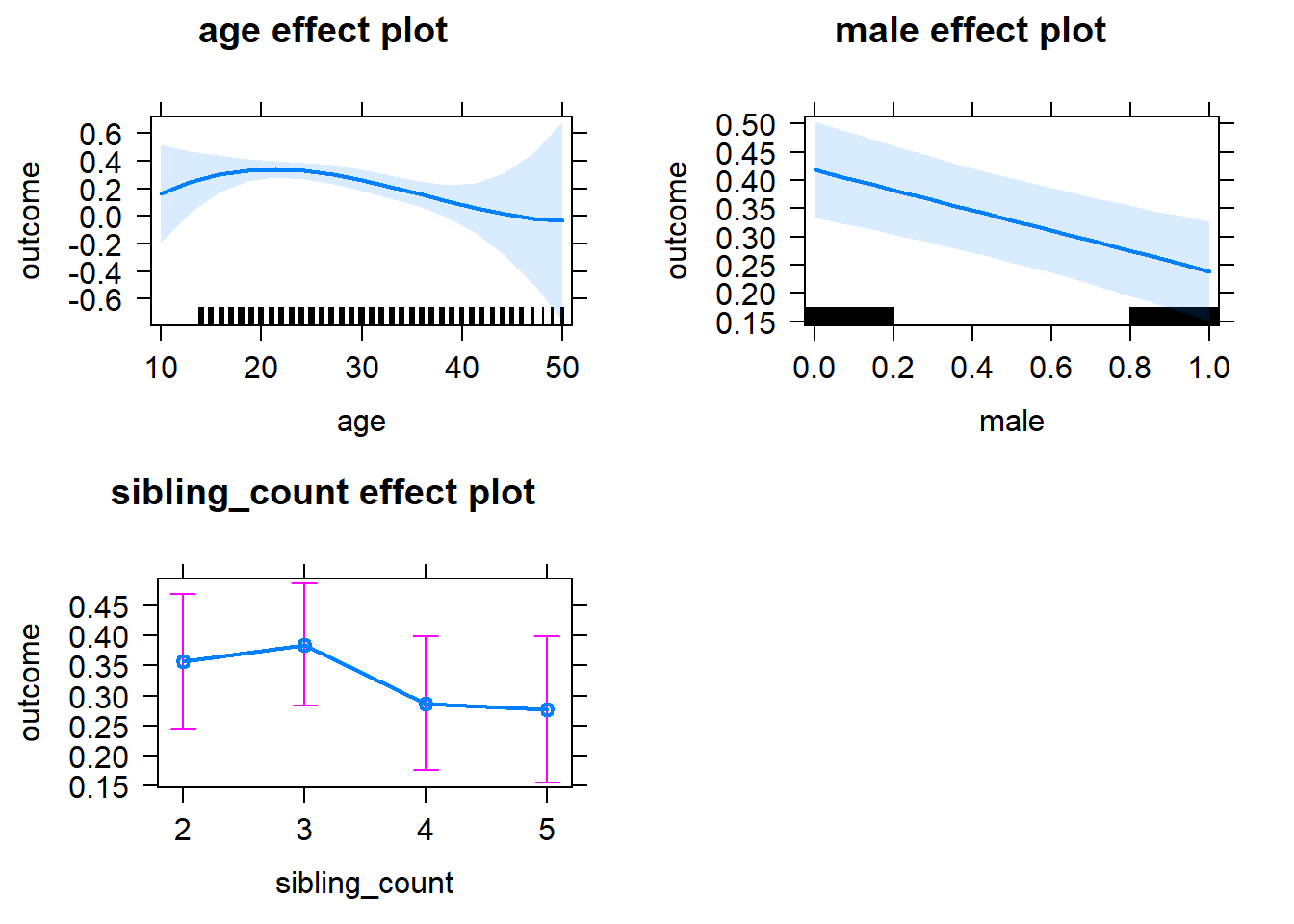
Add Birth Order Linear
Model Summary
tidy(m2_birthorder_linear, conf.int = T, conf.level = 0.995)| effect | group | term | estimate | std.error | statistic | df | p.value | conf.low | conf.high |
|---|---|---|---|---|---|---|---|---|---|
| fixed | NA | (Intercept) | -0.3139 | 0.5815 | -0.5398 | 4174 | 0.5893 | -1.946 | 1.318 |
| fixed | NA | birth_order | 0.0009025 | 0.01584 | 0.05696 | 3912 | 0.9546 | -0.04357 | 0.04538 |
| fixed | NA | poly(age, 3, raw = TRUE)1 | 0.08486 | 0.0679 | 1.25 | 4180 | 0.2114 | -0.1057 | 0.2755 |
| fixed | NA | poly(age, 3, raw = TRUE)2 | -0.002855 | 0.002505 | -1.14 | 4184 | 0.2544 | -0.009886 | 0.004176 |
| fixed | NA | poly(age, 3, raw = TRUE)3 | 0.00002629 | 0.00002937 | 0.8952 | 4187 | 0.3707 | -0.00005615 | 0.0001087 |
| fixed | NA | male | -0.1795 | 0.03142 | -5.715 | 4064 | 0.00000001174 | -0.2677 | -0.09136 |
| fixed | NA | sibling_count3 | 0.02722 | 0.04631 | 0.5878 | 3245 | 0.5567 | -0.1028 | 0.1572 |
| fixed | NA | sibling_count4 | -0.07169 | 0.05111 | -1.403 | 3102 | 0.1608 | -0.2152 | 0.07178 |
| fixed | NA | sibling_count5 | -0.08197 | 0.05825 | -1.407 | 3071 | 0.1595 | -0.2455 | 0.08155 |
| ran_pars | mother_pidlink | sd__(Intercept) | 0.4433 | NA | NA | NA | NA | NA | NA |
| ran_pars | Residual | sd__Observation | 0.93 | NA | NA | NA | NA | NA | NA |
Coefficient Plot
plot_birthorder2(m2_birthorder_linear, separate = FALSE)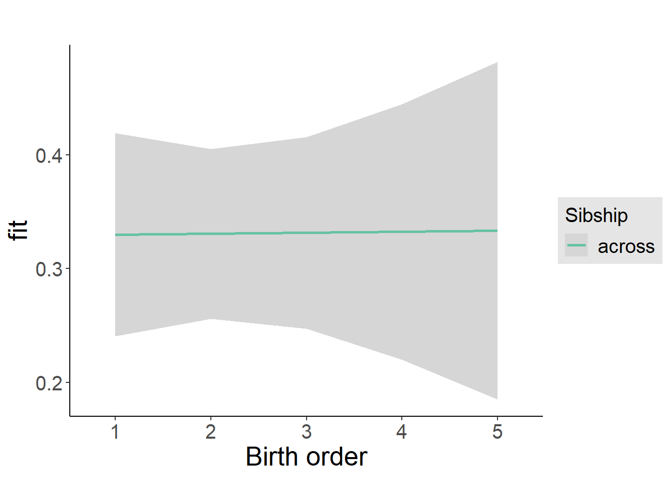
Add Birth Order Factor
Model Summary
m3_birthorder_nonlinear = update(m1_covariates_only, formula = . ~ . + birth_order_nonlinear)
tidy(m3_birthorder_nonlinear, conf.int = T, conf.level = 0.995)| effect | group | term | estimate | std.error | statistic | df | p.value | conf.low | conf.high |
|---|---|---|---|---|---|---|---|---|---|
| fixed | NA | (Intercept) | -0.3432 | 0.5824 | -0.5893 | 4178 | 0.5557 | -1.978 | 1.292 |
| fixed | NA | poly(age, 3, raw = TRUE)1 | 0.08818 | 0.068 | 1.297 | 4181 | 0.1948 | -0.1027 | 0.279 |
| fixed | NA | poly(age, 3, raw = TRUE)2 | -0.002974 | 0.002508 | -1.186 | 4184 | 0.2358 | -0.01002 | 0.004067 |
| fixed | NA | poly(age, 3, raw = TRUE)3 | 0.00002758 | 0.00002941 | 0.9376 | 4186 | 0.3485 | -0.00005498 | 0.0001101 |
| fixed | NA | male | -0.1794 | 0.03142 | -5.71 | 4060 | 0.00000001211 | -0.2676 | -0.09122 |
| fixed | NA | sibling_count3 | 0.01714 | 0.04695 | 0.3651 | 3336 | 0.715 | -0.1147 | 0.1489 |
| fixed | NA | sibling_count4 | -0.07655 | 0.0518 | -1.478 | 3185 | 0.1395 | -0.222 | 0.06885 |
| fixed | NA | sibling_count5 | -0.07804 | 0.05886 | -1.326 | 3120 | 0.185 | -0.2433 | 0.08718 |
| fixed | NA | birth_order_nonlinear2 | 0.007457 | 0.03712 | 0.2009 | 3372 | 0.8408 | -0.09675 | 0.1117 |
| fixed | NA | birth_order_nonlinear3 | 0.04764 | 0.04706 | 1.012 | 3566 | 0.3114 | -0.08446 | 0.1797 |
| fixed | NA | birth_order_nonlinear4 | -0.01793 | 0.06241 | -0.2873 | 3709 | 0.7739 | -0.1931 | 0.1572 |
| fixed | NA | birth_order_nonlinear5 | -0.03863 | 0.09104 | -0.4243 | 3591 | 0.6714 | -0.2942 | 0.2169 |
| ran_pars | mother_pidlink | sd__(Intercept) | 0.444 | NA | NA | NA | NA | NA | NA |
| ran_pars | Residual | sd__Observation | 0.9299 | NA | NA | NA | NA | NA | NA |
Coefficient Plot
plot_birthorder(m3_birthorder_nonlinear, separate = FALSE)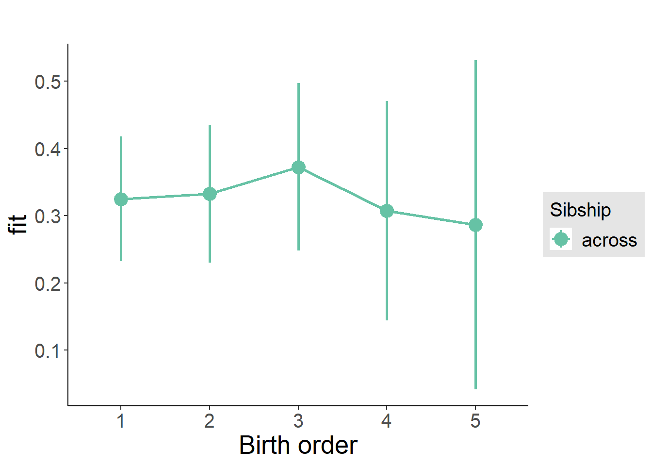
Add Interaction
Model Summary
m4_interaction = update(m3_birthorder_nonlinear, formula = . ~ . - birth_order_nonlinear - sibling_count + count_birth_order)
tidy(m4_interaction, conf.int = T, conf.level = 0.995)| effect | group | term | estimate | std.error | statistic | df | p.value | conf.low | conf.high |
|---|---|---|---|---|---|---|---|---|---|
| fixed | NA | (Intercept) | -0.3502 | 0.5828 | -0.6008 | 4172 | 0.548 | -1.986 | 1.286 |
| fixed | NA | poly(age, 3, raw = TRUE)1 | 0.08616 | 0.06802 | 1.267 | 4174 | 0.2054 | -0.1048 | 0.2771 |
| fixed | NA | poly(age, 3, raw = TRUE)2 | -0.002888 | 0.00251 | -1.151 | 4178 | 0.2499 | -0.009933 | 0.004157 |
| fixed | NA | poly(age, 3, raw = TRUE)3 | 0.00002645 | 0.00002943 | 0.8987 | 4180 | 0.3689 | -0.00005616 | 0.0001091 |
| fixed | NA | male | -0.1812 | 0.03144 | -5.763 | 4053 | 0.000000008881 | -0.2695 | -0.09295 |
| fixed | NA | count_birth_order2/2 | 0.07487 | 0.06719 | 1.114 | 3587 | 0.2652 | -0.1137 | 0.2635 |
| fixed | NA | count_birth_order1/3 | 0.06736 | 0.05962 | 1.13 | 4164 | 0.2587 | -0.1 | 0.2347 |
| fixed | NA | count_birth_order2/3 | 0.0078 | 0.0644 | 0.1211 | 4180 | 0.9036 | -0.173 | 0.1886 |
| fixed | NA | count_birth_order3/3 | 0.08895 | 0.07246 | 1.227 | 4175 | 0.2197 | -0.1145 | 0.2924 |
| fixed | NA | count_birth_order1/4 | -0.09565 | 0.0703 | -1.361 | 4177 | 0.1737 | -0.293 | 0.1017 |
| fixed | NA | count_birth_order2/4 | -0.03206 | 0.07184 | -0.4462 | 4180 | 0.6555 | -0.2337 | 0.1696 |
| fixed | NA | count_birth_order3/4 | -0.02432 | 0.07831 | -0.3106 | 4155 | 0.7561 | -0.2441 | 0.1955 |
| fixed | NA | count_birth_order4/4 | -0.007524 | 0.08077 | -0.09315 | 4156 | 0.9258 | -0.2343 | 0.2192 |
| fixed | NA | count_birth_order1/5 | 0.006059 | 0.08367 | 0.07241 | 4180 | 0.9423 | -0.2288 | 0.2409 |
| fixed | NA | count_birth_order2/5 | -0.06487 | 0.08993 | -0.7213 | 4146 | 0.4708 | -0.3173 | 0.1876 |
| fixed | NA | count_birth_order3/5 | 0.01195 | 0.08712 | 0.1371 | 4141 | 0.8909 | -0.2326 | 0.2565 |
| fixed | NA | count_birth_order4/5 | -0.1584 | 0.09015 | -1.757 | 4119 | 0.07903 | -0.4115 | 0.09468 |
| fixed | NA | count_birth_order5/5 | -0.09581 | 0.08987 | -1.066 | 4123 | 0.2865 | -0.3481 | 0.1565 |
| ran_pars | mother_pidlink | sd__(Intercept) | 0.4436 | NA | NA | NA | NA | NA | NA |
| ran_pars | Residual | sd__Observation | 0.9301 | NA | NA | NA | NA | NA | NA |
Coefficient Plot
plot_birthorder(m4_interaction)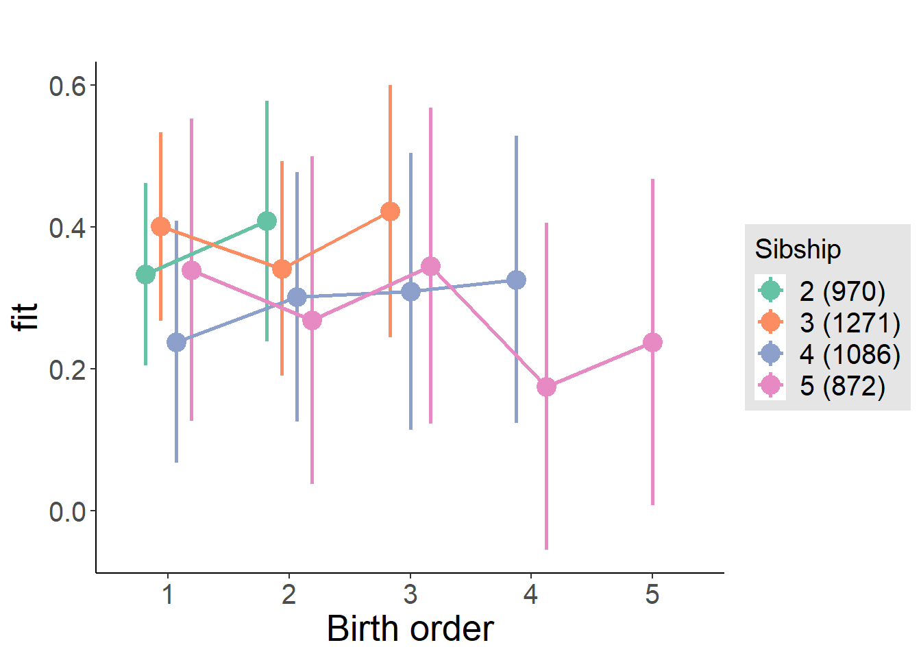
Model Comparison
###### Model 1 - Model 2
anova(m1_covariates_only, m2_birthorder_linear, m3_birthorder_nonlinear, m4_interaction)
## refitting model(s) with ML (instead of REML)| Df | AIC | BIC | logLik | deviance | Chisq | Chi Df | Pr(>Chisq) |
|---|---|---|---|---|---|---|---|
| 10 | 12125 | 12188 | -6052 | 12105 | NA | NA | NA |
| 11 | 12127 | 12197 | -6052 | 12105 | 0.003311 | 1 | 0.9541 |
| 14 | 12131 | 12220 | -6052 | 12103 | 1.742 | 3 | 0.6276 |
| 20 | 12137 | 12264 | -6049 | 12097 | 5.854 | 6 | 0.4397 |
Parental full sibling order
outcome_parental_m1 <- update(m2_birthorder_linear, data = birthorder %>%
  mutate(sibling_count = sibling_count_genes_factor,
         birth_order_nonlinear = birthorder_genes_factor,
         birth_order = birthorder_genes,
         count_birth_order = count_birthorder_genes
         ) %>%
      filter(sibling_count != "1"))
compare_models_markdown(outcome_parental_m1)
Basic Model
Model Summary
m1_covariates_only <- update(m2_birthorder_linear, formula = . ~ . - birth_order)
tidy(m1_covariates_only, conf.int = T, conf.level = 0.995)| effect | group | term | estimate | std.error | statistic | df | p.value | conf.low | conf.high |
|---|---|---|---|---|---|---|---|---|---|
| fixed | NA | (Intercept) | -0.416 | 0.5686 | -0.7316 | 4479 | 0.4645 | -2.012 | 1.18 |
| fixed | NA | poly(age, 3, raw = TRUE)1 | 0.09561 | 0.06648 | 1.438 | 4485 | 0.1505 | -0.091 | 0.2822 |
| fixed | NA | poly(age, 3, raw = TRUE)2 | -0.003242 | 0.002455 | -1.321 | 4490 | 0.1867 | -0.01013 | 0.003649 |
| fixed | NA | poly(age, 3, raw = TRUE)3 | 0.00003082 | 0.00002883 | 1.069 | 4493 | 0.2851 | -0.00005011 | 0.0001118 |
| fixed | NA | male | -0.1756 | 0.03027 | -5.802 | 4364 | 0.000000007033 | -0.2606 | -0.09066 |
| fixed | NA | sibling_count3 | 0.01526 | 0.04177 | 0.3653 | 3358 | 0.7149 | -0.102 | 0.1325 |
| fixed | NA | sibling_count4 | -0.0601 | 0.04552 | -1.32 | 3026 | 0.1868 | -0.1879 | 0.06767 |
| fixed | NA | sibling_count5 | -0.1183 | 0.05401 | -2.19 | 2686 | 0.02858 | -0.2699 | 0.03331 |
| ran_pars | mother_pidlink | sd__(Intercept) | 0.4493 | NA | NA | NA | NA | NA | NA |
| ran_pars | Residual | sd__Observation | 0.9259 | NA | NA | NA | NA | NA | NA |
Coefficient Plot
plot(allEffects(m1_covariates_only, confidence.level = 0.995))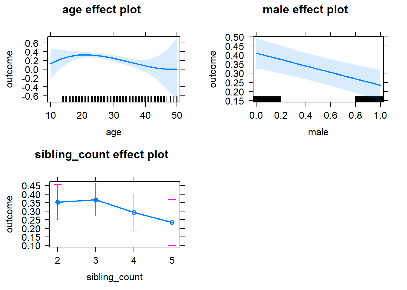
Add Birth Order Linear
Model Summary
tidy(m2_birthorder_linear, conf.int = T, conf.level = 0.995)| effect | group | term | estimate | std.error | statistic | df | p.value | conf.low | conf.high |
|---|---|---|---|---|---|---|---|---|---|
| fixed | NA | (Intercept) | -0.4442 | 0.5692 | -0.7804 | 4479 | 0.4352 | -2.042 | 1.154 |
| fixed | NA | birth_order | 0.01691 | 0.01597 | 1.058 | 4084 | 0.2899 | -0.02793 | 0.06174 |
| fixed | NA | poly(age, 3, raw = TRUE)1 | 0.09643 | 0.06649 | 1.45 | 4484 | 0.147 | -0.09019 | 0.2831 |
| fixed | NA | poly(age, 3, raw = TRUE)2 | -0.003288 | 0.002455 | -1.339 | 4489 | 0.1806 | -0.01018 | 0.003604 |
| fixed | NA | poly(age, 3, raw = TRUE)3 | 0.00003171 | 0.00002884 | 1.099 | 4492 | 0.2717 | -0.00004926 | 0.0001127 |
| fixed | NA | male | -0.1762 | 0.03028 | -5.819 | 4362 | 0.000000006345 | -0.2612 | -0.0912 |
| fixed | NA | sibling_count3 | 0.007398 | 0.04243 | 0.1744 | 3410 | 0.8616 | -0.1117 | 0.1265 |
| fixed | NA | sibling_count4 | -0.07811 | 0.04859 | -1.607 | 3246 | 0.1081 | -0.2145 | 0.05829 |
| fixed | NA | sibling_count5 | -0.1472 | 0.06049 | -2.432 | 3120 | 0.01505 | -0.317 | 0.02266 |
| ran_pars | mother_pidlink | sd__(Intercept) | 0.4491 | NA | NA | NA | NA | NA | NA |
| ran_pars | Residual | sd__Observation | 0.926 | NA | NA | NA | NA | NA | NA |
Coefficient Plot
plot_birthorder2(m2_birthorder_linear, separate = FALSE)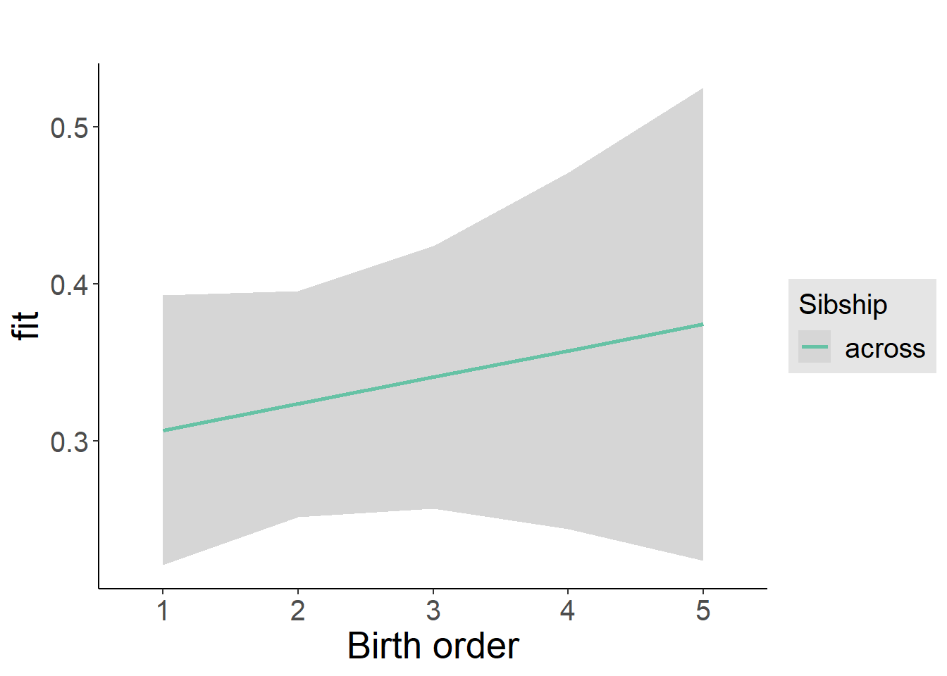
Add Birth Order Factor
Model Summary
m3_birthorder_nonlinear = update(m1_covariates_only, formula = . ~ . + birth_order_nonlinear)
tidy(m3_birthorder_nonlinear, conf.int = T, conf.level = 0.995)| effect | group | term | estimate | std.error | statistic | df | p.value | conf.low | conf.high |
|---|---|---|---|---|---|---|---|---|---|
| fixed | NA | (Intercept) | -0.432 | 0.5701 | -0.7577 | 4482 | 0.4487 | -2.032 | 1.168 |
| fixed | NA | poly(age, 3, raw = TRUE)1 | 0.09753 | 0.06659 | 1.465 | 4485 | 0.1431 | -0.0894 | 0.2845 |
| fixed | NA | poly(age, 3, raw = TRUE)2 | -0.003326 | 0.002459 | -1.353 | 4488 | 0.1763 | -0.01023 | 0.003577 |
| fixed | NA | poly(age, 3, raw = TRUE)3 | 0.00003209 | 0.00002888 | 1.111 | 4490 | 0.2665 | -0.00004897 | 0.0001132 |
| fixed | NA | male | -0.1758 | 0.03029 | -5.805 | 4358 | 0.000000006895 | -0.2609 | -0.09081 |
| fixed | NA | sibling_count3 | -0.000006417 | 0.04307 | -0.000149 | 3523 | 0.9999 | -0.1209 | 0.1209 |
| fixed | NA | sibling_count4 | -0.08365 | 0.0493 | -1.697 | 3342 | 0.08983 | -0.222 | 0.05473 |
| fixed | NA | sibling_count5 | -0.1455 | 0.06168 | -2.358 | 3224 | 0.01841 | -0.3186 | 0.02767 |
| fixed | NA | birth_order_nonlinear2 | 0.002265 | 0.03533 | 0.06411 | 3557 | 0.9489 | -0.0969 | 0.1014 |
| fixed | NA | birth_order_nonlinear3 | 0.06415 | 0.04526 | 1.417 | 3730 | 0.1564 | -0.06289 | 0.1912 |
| fixed | NA | birth_order_nonlinear4 | 0.0386 | 0.06249 | 0.6177 | 3905 | 0.5368 | -0.1368 | 0.214 |
| fixed | NA | birth_order_nonlinear5 | 0.02918 | 0.102 | 0.2862 | 3814 | 0.7748 | -0.257 | 0.3154 |
| ran_pars | mother_pidlink | sd__(Intercept) | 0.4493 | NA | NA | NA | NA | NA | NA |
| ran_pars | Residual | sd__Observation | 0.9262 | NA | NA | NA | NA | NA | NA |
Coefficient Plot
plot_birthorder(m3_birthorder_nonlinear, separate = FALSE)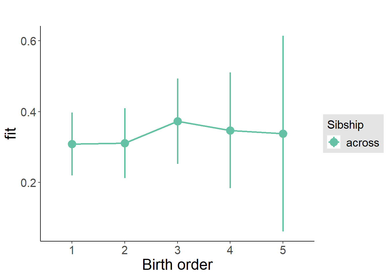
Add Interaction
Model Summary
m4_interaction = update(m3_birthorder_nonlinear, formula = . ~ . - birth_order_nonlinear - sibling_count + count_birth_order)
tidy(m4_interaction, conf.int = T, conf.level = 0.995)| effect | group | term | estimate | std.error | statistic | df | p.value | conf.low | conf.high |
|---|---|---|---|---|---|---|---|---|---|
| fixed | NA | (Intercept) | -0.4268 | 0.5705 | -0.7481 | 4476 | 0.4545 | -2.028 | 1.175 |
| fixed | NA | poly(age, 3, raw = TRUE)1 | 0.0961 | 0.06663 | 1.442 | 4478 | 0.1493 | -0.09094 | 0.2831 |
| fixed | NA | poly(age, 3, raw = TRUE)2 | -0.00326 | 0.002461 | -1.325 | 4482 | 0.1852 | -0.01017 | 0.003647 |
| fixed | NA | poly(age, 3, raw = TRUE)3 | 0.00003118 | 0.0000289 | 1.079 | 4484 | 0.2807 | -0.00004995 | 0.0001123 |
| fixed | NA | male | -0.1759 | 0.03031 | -5.802 | 4351 | 0.000000007003 | -0.261 | -0.0908 |
| fixed | NA | count_birth_order2/2 | 0.01494 | 0.05951 | 0.251 | 3756 | 0.8018 | -0.1521 | 0.182 |
| fixed | NA | count_birth_order1/3 | 0.006263 | 0.05435 | 0.1152 | 4464 | 0.9083 | -0.1463 | 0.1588 |
| fixed | NA | count_birth_order2/3 | 0.009709 | 0.05978 | 0.1624 | 4486 | 0.871 | -0.1581 | 0.1775 |
| fixed | NA | count_birth_order3/3 | 0.06011 | 0.06564 | 0.9157 | 4477 | 0.3599 | -0.1241 | 0.2444 |
| fixed | NA | count_birth_order1/4 | -0.08948 | 0.06739 | -1.328 | 4485 | 0.1843 | -0.2787 | 0.0997 |
| fixed | NA | count_birth_order2/4 | -0.1179 | 0.06945 | -1.697 | 4480 | 0.08976 | -0.3128 | 0.07709 |
| fixed | NA | count_birth_order3/4 | 0.002842 | 0.07238 | 0.03927 | 4458 | 0.9687 | -0.2003 | 0.206 |
| fixed | NA | count_birth_order4/4 | 0.006872 | 0.07627 | 0.0901 | 4446 | 0.9282 | -0.2072 | 0.221 |
| fixed | NA | count_birth_order1/5 | -0.1059 | 0.09127 | -1.16 | 4480 | 0.246 | -0.3621 | 0.1503 |
| fixed | NA | count_birth_order2/5 | -0.07683 | 0.1007 | -0.7631 | 4416 | 0.4454 | -0.3595 | 0.2058 |
| fixed | NA | count_birth_order3/5 | -0.09122 | 0.09563 | -0.9539 | 4419 | 0.3402 | -0.3597 | 0.1772 |
| fixed | NA | count_birth_order4/5 | -0.1786 | 0.09266 | -1.928 | 4437 | 0.05395 | -0.4387 | 0.08148 |
| fixed | NA | count_birth_order5/5 | -0.1131 | 0.09776 | -1.157 | 4416 | 0.2474 | -0.3875 | 0.1613 |
| ran_pars | mother_pidlink | sd__(Intercept) | 0.4486 | NA | NA | NA | NA | NA | NA |
| ran_pars | Residual | sd__Observation | 0.9269 | NA | NA | NA | NA | NA | NA |
Coefficient Plot
plot_birthorder(m4_interaction)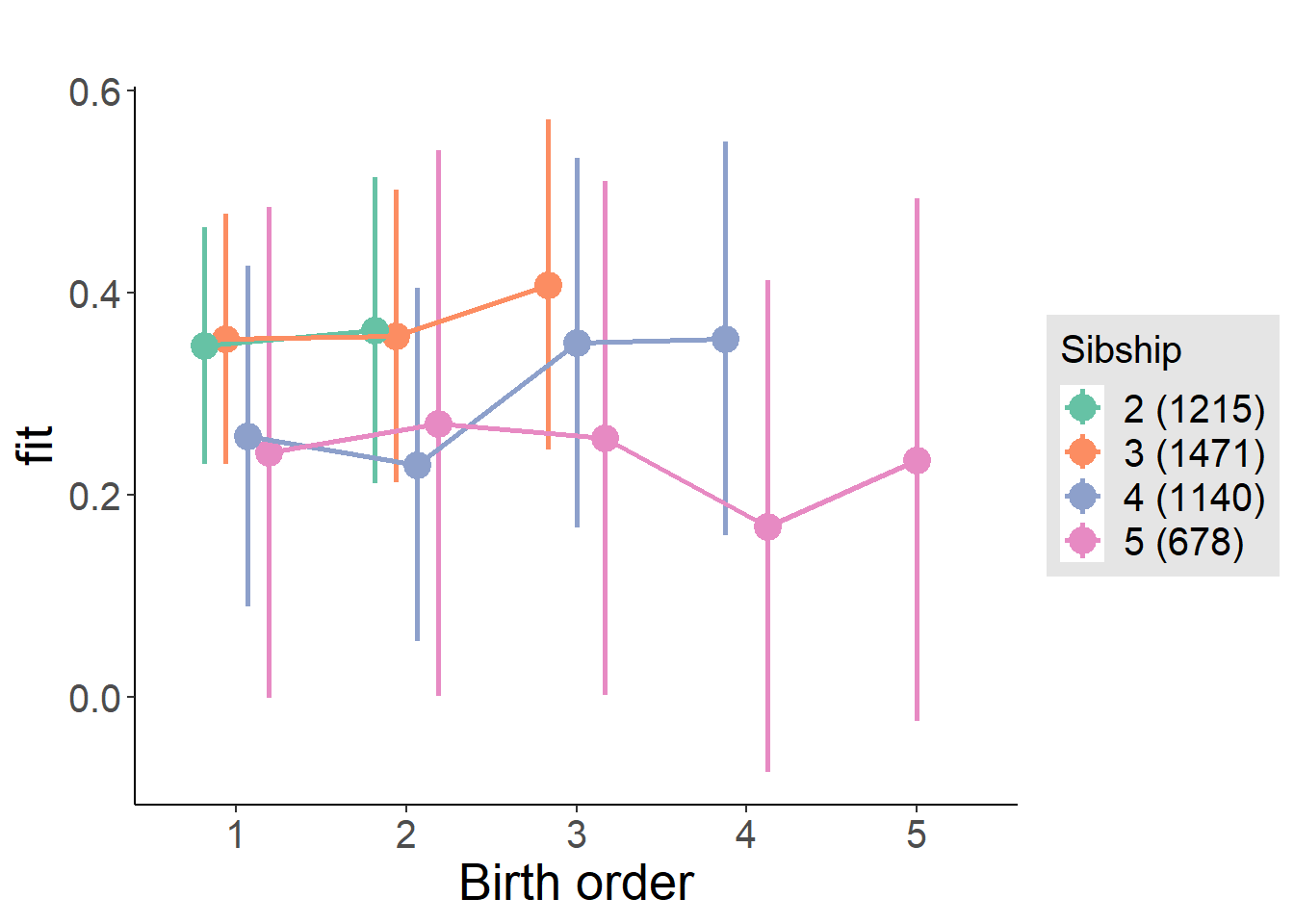
Model Comparison
###### Model 1 - Model 2
anova(m1_covariates_only, m2_birthorder_linear, m3_birthorder_nonlinear, m4_interaction)
## refitting model(s) with ML (instead of REML)| Df | AIC | BIC | logLik | deviance | Chisq | Chi Df | Pr(>Chisq) |
|---|---|---|---|---|---|---|---|
| 10 | 12991 | 13055 | -6485 | 12971 | NA | NA | NA |
| 11 | 12992 | 13062 | -6485 | 12970 | 1.123 | 1 | 0.2894 |
| 14 | 12997 | 13086 | -6484 | 12969 | 1.185 | 3 | 0.7566 |
| 20 | 13006 | 13134 | -6483 | 12966 | 2.819 | 6 | 0.8312 |
Compare birth order specifications
library(coefplot)
multiplot(outcome_naive_m1, outcome_preg_m1, outcome_uterus_m1, outcome_parental_m1, dodgeHeight = 0.6,
          intercept = FALSE)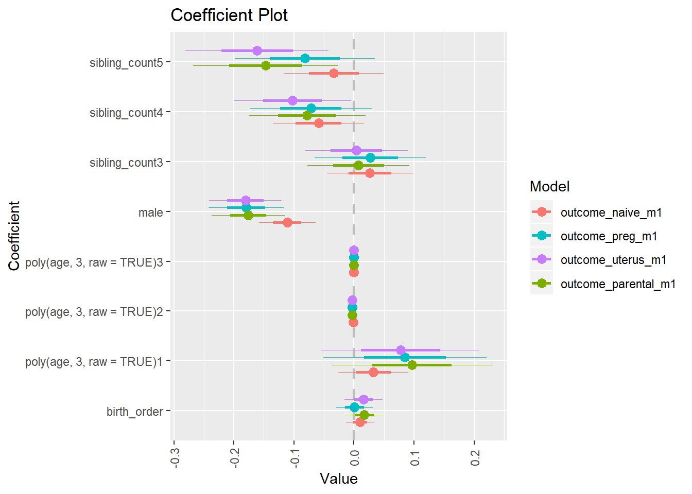
Raven 2015 young
birthorder <- birthorder %>% mutate(outcome = raven_2015_young)
model = lmer(outcome ~ birth_order + poly(age, 3, raw = TRUE) + male + sibling_count + (1 | mother_pidlink),
                   data = birthorder)
compare_birthorder_specs(model)
Naive birth order
outcome_naive_m1 <- update(m2_birthorder_linear, data = birthorder %>%
                     mutate(sibling_count = sibling_count_naive_factor,
                            birth_order_nonlinear = birthorder_naive_factor,
                            birth_order = birthorder_naive,
                            count_birth_order = count_birthorder_naive) %>%
                     filter(sibling_count != "1"))
compare_models_markdown(outcome_naive_m1)
Basic Model
Model Summary
m1_covariates_only <- update(m2_birthorder_linear, formula = . ~ . - birth_order)
tidy(m1_covariates_only, conf.int = T, conf.level = 0.995)| effect | group | term | estimate | std.error | statistic | df | p.value | conf.low | conf.high |
|---|---|---|---|---|---|---|---|---|---|
| fixed | NA | (Intercept) | -2.822 | 0.1249 | -22.6 | 7834 | 1.451e-109 | -3.172 | -2.471 |
| fixed | NA | poly(age, 3, raw = TRUE)1 | 0.4021 | 0.02318 | 17.35 | 8001 | 3.445e-66 | 0.337 | 0.4671 |
| fixed | NA | poly(age, 3, raw = TRUE)2 | -0.01567 | 0.001335 | -11.74 | 8131 | 1.449e-31 | -0.01942 | -0.01192 |
| fixed | NA | poly(age, 3, raw = TRUE)3 | 0.0001864 | 0.00002434 | 7.66 | 8084 | 2.069e-14 | 0.0001181 | 0.0002547 |
| fixed | NA | male | 0.04525 | 0.01952 | 2.319 | 7411 | 0.02044 | -0.009532 | 0.1 |
| fixed | NA | sibling_count3 | -0.03604 | 0.02829 | -1.274 | 5234 | 0.2027 | -0.1155 | 0.04337 |
| fixed | NA | sibling_count4 | -0.09036 | 0.03188 | -2.835 | 4779 | 0.004606 | -0.1798 | -0.0008817 |
| fixed | NA | sibling_count5 | -0.07959 | 0.03619 | -2.199 | 4357 | 0.0279 | -0.1812 | 0.02199 |
| ran_pars | mother_pidlink | sd__(Intercept) | 0.5239 | NA | NA | NA | NA | NA | NA |
| ran_pars | Residual | sd__Observation | 0.755 | NA | NA | NA | NA | NA | NA |
Coefficient Plot
plot(allEffects(m1_covariates_only, confidence.level = 0.995))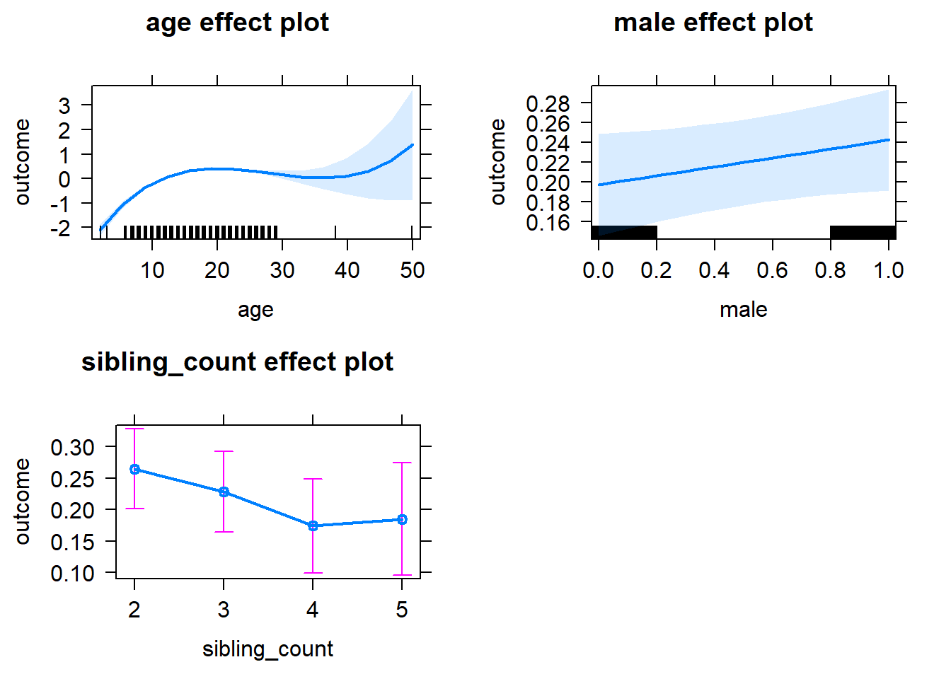
Add Birth Order Linear
Model Summary
tidy(m2_birthorder_linear, conf.int = T, conf.level = 0.995)| effect | group | term | estimate | std.error | statistic | df | p.value | conf.low | conf.high |
|---|---|---|---|---|---|---|---|---|---|
| fixed | NA | (Intercept) | -2.811 | 0.1281 | -21.95 | 7938 | 9.899e-104 | -3.17 | -2.451 |
| fixed | NA | birth_order | -0.004207 | 0.01077 | -0.3905 | 7575 | 0.6962 | -0.03445 | 0.02604 |
| fixed | NA | poly(age, 3, raw = TRUE)1 | 0.4014 | 0.02324 | 17.27 | 8007 | 1.187e-65 | 0.3362 | 0.4667 |
| fixed | NA | poly(age, 3, raw = TRUE)2 | -0.01565 | 0.001336 | -11.72 | 8129 | 1.818e-31 | -0.0194 | -0.0119 |
| fixed | NA | poly(age, 3, raw = TRUE)3 | 0.0001863 | 0.00002434 | 7.653 | 8085 | 2.183e-14 | 0.000118 | 0.0002546 |
| fixed | NA | male | 0.0453 | 0.01952 | 2.321 | 7410 | 0.0203 | -0.009479 | 0.1001 |
| fixed | NA | sibling_count3 | -0.03363 | 0.02896 | -1.161 | 5354 | 0.2456 | -0.1149 | 0.04767 |
| fixed | NA | sibling_count4 | -0.08459 | 0.03513 | -2.408 | 5192 | 0.01608 | -0.1832 | 0.01402 |
| fixed | NA | sibling_count5 | -0.07027 | 0.04335 | -1.621 | 5149 | 0.1051 | -0.192 | 0.05143 |
| ran_pars | mother_pidlink | sd__(Intercept) | 0.5239 | NA | NA | NA | NA | NA | NA |
| ran_pars | Residual | sd__Observation | 0.755 | NA | NA | NA | NA | NA | NA |
Coefficient Plot
plot_birthorder2(m2_birthorder_linear, separate = FALSE)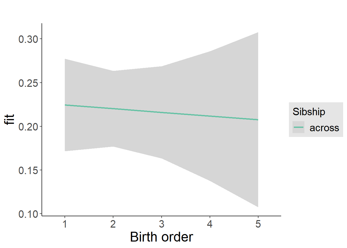
Add Birth Order Factor
Model Summary
m3_birthorder_nonlinear = update(m1_covariates_only, formula = . ~ . + birth_order_nonlinear)
tidy(m3_birthorder_nonlinear, conf.int = T, conf.level = 0.995)| effect | group | term | estimate | std.error | statistic | df | p.value | conf.low | conf.high |
|---|---|---|---|---|---|---|---|---|---|
| fixed | NA | (Intercept) | -2.824 | 0.1267 | -22.29 | 7934 | 9.056e-107 | -3.18 | -2.469 |
| fixed | NA | poly(age, 3, raw = TRUE)1 | 0.4024 | 0.02327 | 17.29 | 8018 | 8.72e-66 | 0.337 | 0.4677 |
| fixed | NA | poly(age, 3, raw = TRUE)2 | -0.0157 | 0.001337 | -11.74 | 8128 | 1.425e-31 | -0.01945 | -0.01194 |
| fixed | NA | poly(age, 3, raw = TRUE)3 | 0.0001868 | 0.00002435 | 7.671 | 8079 | 1.899e-14 | 0.0001185 | 0.0002552 |
| fixed | NA | male | 0.04507 | 0.01952 | 2.309 | 7408 | 0.02099 | -0.009729 | 0.09986 |
| fixed | NA | sibling_count3 | -0.03865 | 0.02943 | -1.313 | 5582 | 0.1891 | -0.1213 | 0.04395 |
| fixed | NA | sibling_count4 | -0.08783 | 0.03582 | -2.452 | 5455 | 0.01423 | -0.1884 | 0.01271 |
| fixed | NA | sibling_count5 | -0.06417 | 0.04397 | -1.459 | 5278 | 0.1445 | -0.1876 | 0.05926 |
| fixed | NA | birth_order_nonlinear2 | 0.006981 | 0.02273 | 0.3072 | 5825 | 0.7587 | -0.05681 | 0.07077 |
| fixed | NA | birth_order_nonlinear3 | 0.01078 | 0.02997 | 0.3599 | 6579 | 0.719 | -0.07334 | 0.09491 |
| fixed | NA | birth_order_nonlinear4 | -0.01946 | 0.04063 | -0.4788 | 6819 | 0.6321 | -0.1335 | 0.0946 |
| fixed | NA | birth_order_nonlinear5 | -0.04141 | 0.05901 | -0.7017 | 6939 | 0.4829 | -0.2071 | 0.1242 |
| ran_pars | mother_pidlink | sd__(Intercept) | 0.5241 | NA | NA | NA | NA | NA | NA |
| ran_pars | Residual | sd__Observation | 0.755 | NA | NA | NA | NA | NA | NA |
Coefficient Plot
plot_birthorder(m3_birthorder_nonlinear, separate = FALSE)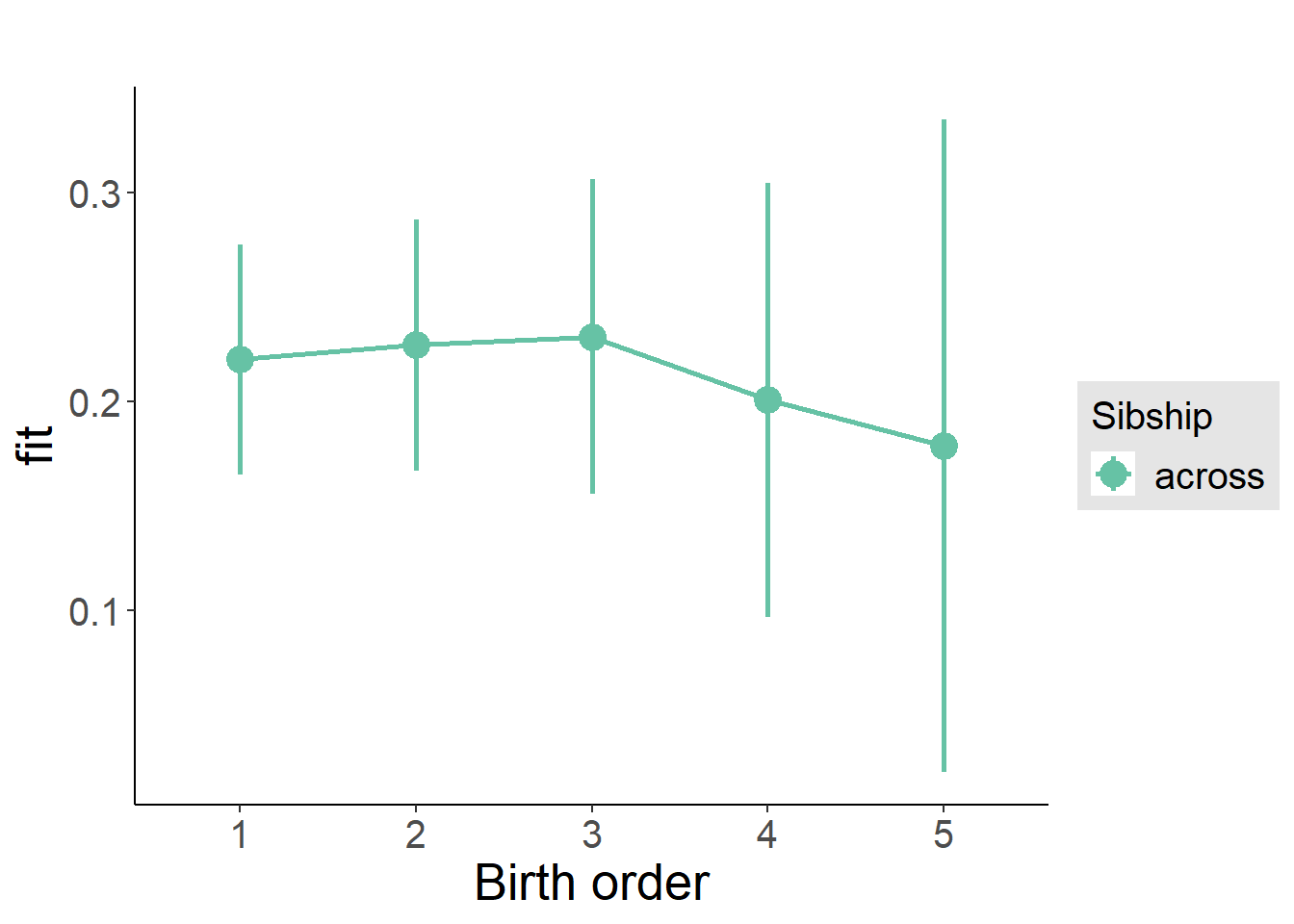
Add Interaction
Model Summary
m4_interaction = update(m3_birthorder_nonlinear, formula = . ~ . - birth_order_nonlinear - sibling_count + count_birth_order)
tidy(m4_interaction, conf.int = T, conf.level = 0.995)| effect | group | term | estimate | std.error | statistic | df | p.value | conf.low | conf.high |
|---|---|---|---|---|---|---|---|---|---|
| fixed | NA | (Intercept) | -2.827 | 0.1276 | -22.16 | 7951 | 1.214e-105 | -3.185 | -2.469 |
| fixed | NA | poly(age, 3, raw = TRUE)1 | 0.4038 | 0.0233 | 17.33 | 8023 | 4.361e-66 | 0.3384 | 0.4692 |
| fixed | NA | poly(age, 3, raw = TRUE)2 | -0.01579 | 0.001338 | -11.8 | 8122 | 7.326e-32 | -0.01954 | -0.01203 |
| fixed | NA | poly(age, 3, raw = TRUE)3 | 0.0001884 | 0.00002437 | 7.733 | 8073 | 1.178e-14 | 0.00012 | 0.0002568 |
| fixed | NA | male | 0.04432 | 0.01952 | 2.271 | 7402 | 0.02318 | -0.01046 | 0.0991 |
| fixed | NA | count_birth_order2/2 | -0.004487 | 0.03564 | -0.1259 | 6126 | 0.8998 | -0.1045 | 0.09554 |
| fixed | NA | count_birth_order1/3 | -0.06921 | 0.03678 | -1.882 | 8000 | 0.05991 | -0.1725 | 0.03404 |
| fixed | NA | count_birth_order2/3 | -0.0402 | 0.03743 | -1.074 | 8073 | 0.2828 | -0.1453 | 0.06486 |
| fixed | NA | count_birth_order3/3 | 0.02043 | 0.04235 | 0.4825 | 8124 | 0.6295 | -0.09845 | 0.1393 |
| fixed | NA | count_birth_order1/4 | -0.07409 | 0.05038 | -1.471 | 8115 | 0.1414 | -0.2155 | 0.06734 |
| fixed | NA | count_birth_order2/4 | -0.04536 | 0.04774 | -0.9502 | 8113 | 0.342 | -0.1794 | 0.08865 |
| fixed | NA | count_birth_order3/4 | -0.1553 | 0.04489 | -3.459 | 8124 | 0.0005452 | -0.2813 | -0.02926 |
| fixed | NA | count_birth_order4/4 | -0.07482 | 0.04893 | -1.529 | 8097 | 0.1263 | -0.2122 | 0.06253 |
| fixed | NA | count_birth_order1/5 | 0.002788 | 0.06832 | 0.04081 | 7756 | 0.9674 | -0.189 | 0.1946 |
| fixed | NA | count_birth_order2/5 | -0.09213 | 0.06488 | -1.42 | 7840 | 0.1557 | -0.2742 | 0.08999 |
| fixed | NA | count_birth_order3/5 | -0.02168 | 0.05868 | -0.3695 | 7996 | 0.7118 | -0.1864 | 0.143 |
| fixed | NA | count_birth_order4/5 | -0.1349 | 0.05514 | -2.448 | 8081 | 0.0144 | -0.2897 | 0.01982 |
| fixed | NA | count_birth_order5/5 | -0.109 | 0.05466 | -1.994 | 8104 | 0.04617 | -0.2624 | 0.04443 |
| ran_pars | mother_pidlink | sd__(Intercept) | 0.5244 | NA | NA | NA | NA | NA | NA |
| ran_pars | Residual | sd__Observation | 0.7544 | NA | NA | NA | NA | NA | NA |
Coefficient Plot
plot_birthorder(m4_interaction)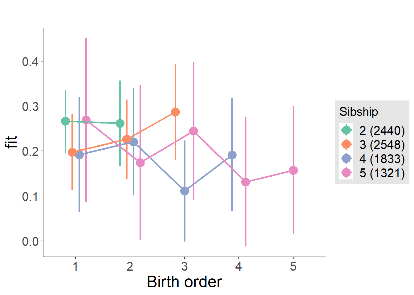
Model Comparison
###### Model 1 - Model 2
anova(m1_covariates_only, m2_birthorder_linear, m3_birthorder_nonlinear, m4_interaction)
## refitting model(s) with ML (instead of REML)| Df | AIC | BIC | logLik | deviance | Chisq | Chi Df | Pr(>Chisq) |
|---|---|---|---|---|---|---|---|
| 10 | 21385 | 21455 | -10683 | 21365 | NA | NA | NA |
| 11 | 21387 | 21464 | -10682 | 21365 | 0.1526 | 1 | 0.6961 |
| 14 | 21392 | 21490 | -10682 | 21364 | 1.06 | 3 | 0.7867 |
| 20 | 21390 | 21531 | -10675 | 21350 | 13.4 | 6 | 0.03716 |
Maternal birth order
outcome_uterus_m1 <- update(m2_birthorder_linear, data = birthorder %>%
                     mutate(sibling_count = sibling_count_uterus_alive_factor,
                            birth_order_nonlinear = birthorder_uterus_alive_factor,
                            birth_order = birthorder_uterus_alive,
                            count_birth_order = count_birthorder_uterus_alive) %>%
                     filter(sibling_count != "1"))
compare_models_markdown(outcome_uterus_m1)
Basic Model
Model Summary
m1_covariates_only <- update(m2_birthorder_linear, formula = . ~ . - birth_order)
tidy(m1_covariates_only, conf.int = T, conf.level = 0.995)| effect | group | term | estimate | std.error | statistic | df | p.value | conf.low | conf.high |
|---|---|---|---|---|---|---|---|---|---|
| fixed | NA | (Intercept) | -3.19 | 0.2021 | -15.78 | 6316 | 4.42e-55 | -3.758 | -2.623 |
| fixed | NA | poly(age, 3, raw = TRUE)1 | 0.4824 | 0.04241 | 11.37 | 6310 | 1.11e-29 | 0.3633 | 0.6014 |
| fixed | NA | poly(age, 3, raw = TRUE)2 | -0.02082 | 0.002745 | -7.583 | 6356 | 3.851e-14 | -0.02852 | -0.01311 |
| fixed | NA | poly(age, 3, raw = TRUE)3 | 0.0002915 | 0.00005507 | 5.294 | 6401 | 0.0000001238 | 0.0001369 | 0.0004461 |
| fixed | NA | male | 0.03392 | 0.02031 | 1.67 | 6991 | 0.09498 | -0.0231 | 0.09093 |
| fixed | NA | sibling_count3 | -0.05851 | 0.02723 | -2.149 | 4661 | 0.03172 | -0.135 | 0.01793 |
| fixed | NA | sibling_count4 | -0.1176 | 0.03346 | -3.515 | 4059 | 0.0004438 | -0.2116 | -0.02371 |
| fixed | NA | sibling_count5 | -0.2155 | 0.04296 | -5.015 | 3671 | 0.0000005553 | -0.3361 | -0.09486 |
| ran_pars | mother_pidlink | sd__(Intercept) | 0.4977 | NA | NA | NA | NA | NA | NA |
| ran_pars | Residual | sd__Observation | 0.7635 | NA | NA | NA | NA | NA | NA |
Coefficient Plot
plot(allEffects(m1_covariates_only, confidence.level = 0.995))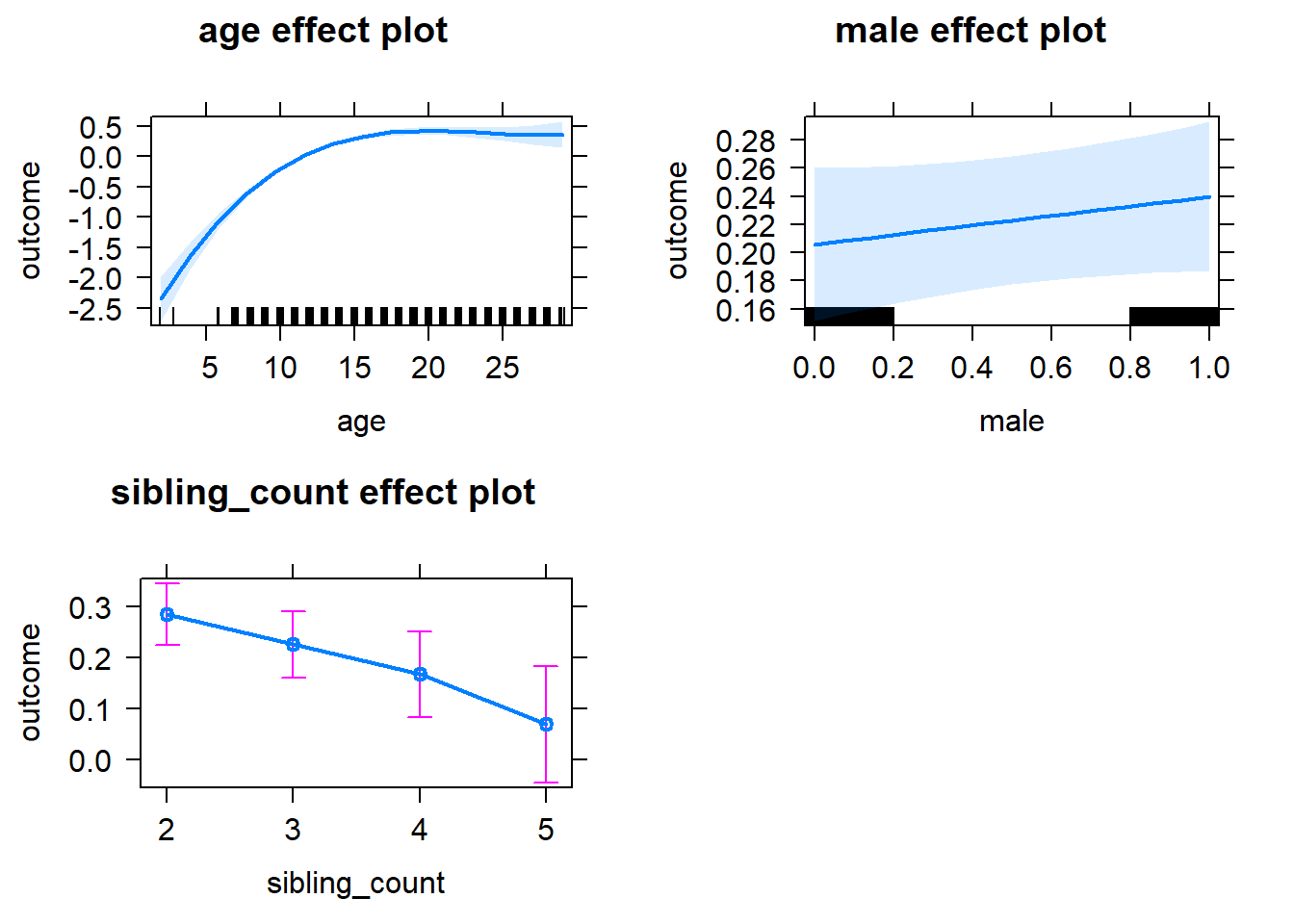
Add Birth Order Linear
Model Summary
tidy(m2_birthorder_linear, conf.int = T, conf.level = 0.995)| effect | group | term | estimate | std.error | statistic | df | p.value | conf.low | conf.high |
|---|---|---|---|---|---|---|---|---|---|
| fixed | NA | (Intercept) | -3.173 | 0.2052 | -15.46 | 6483 | 5.531e-53 | -3.749 | -2.597 |
| fixed | NA | birth_order | -0.006215 | 0.01248 | -0.4979 | 7191 | 0.6186 | -0.04125 | 0.02882 |
| fixed | NA | poly(age, 3, raw = TRUE)1 | 0.4811 | 0.04249 | 11.32 | 6334 | 1.97e-29 | 0.3618 | 0.6004 |
| fixed | NA | poly(age, 3, raw = TRUE)2 | -0.02077 | 0.002747 | -7.561 | 6356 | 4.563e-14 | -0.02848 | -0.01306 |
| fixed | NA | poly(age, 3, raw = TRUE)3 | 0.0002909 | 0.00005508 | 5.281 | 6399 | 0.0000001327 | 0.0001363 | 0.0004455 |
| fixed | NA | male | 0.03404 | 0.02031 | 1.676 | 6993 | 0.09385 | -0.02298 | 0.09106 |
| fixed | NA | sibling_count3 | -0.05439 | 0.02847 | -1.911 | 4774 | 0.05611 | -0.1343 | 0.02552 |
| fixed | NA | sibling_count4 | -0.1084 | 0.03822 | -2.838 | 4515 | 0.004565 | -0.2157 | -0.001169 |
| fixed | NA | sibling_count5 | -0.2002 | 0.05277 | -3.794 | 4559 | 0.0001504 | -0.3483 | -0.05206 |
| ran_pars | mother_pidlink | sd__(Intercept) | 0.4976 | NA | NA | NA | NA | NA | NA |
| ran_pars | Residual | sd__Observation | 0.7636 | NA | NA | NA | NA | NA | NA |
Coefficient Plot
plot_birthorder2(m2_birthorder_linear, separate = FALSE)
Add Birth Order Factor
Model Summary
m3_birthorder_nonlinear = update(m1_covariates_only, formula = . ~ . + birth_order_nonlinear)
tidy(m3_birthorder_nonlinear, conf.int = T, conf.level = 0.995)| effect | group | term | estimate | std.error | statistic | df | p.value | conf.low | conf.high |
|---|---|---|---|---|---|---|---|---|---|
| fixed | NA | (Intercept) | -3.185 | 0.2038 | -15.63 | 6435 | 4.515e-54 | -3.757 | -2.613 |
| fixed | NA | poly(age, 3, raw = TRUE)1 | 0.4815 | 0.04251 | 11.33 | 6338 | 1.847e-29 | 0.3622 | 0.6008 |
| fixed | NA | poly(age, 3, raw = TRUE)2 | -0.02077 | 0.002747 | -7.56 | 6358 | 4.604e-14 | -0.02848 | -0.01306 |
| fixed | NA | poly(age, 3, raw = TRUE)3 | 0.0002906 | 0.00005509 | 5.274 | 6400 | 0.0000001379 | 0.0001359 | 0.0004452 |
| fixed | NA | male | 0.03356 | 0.02032 | 1.652 | 6993 | 0.09866 | -0.02348 | 0.0906 |
| fixed | NA | sibling_count3 | -0.06243 | 0.02915 | -2.141 | 5068 | 0.03229 | -0.1443 | 0.01941 |
| fixed | NA | sibling_count4 | -0.1148 | 0.03914 | -2.932 | 4746 | 0.003386 | -0.2246 | -0.004885 |
| fixed | NA | sibling_count5 | -0.1774 | 0.05539 | -3.203 | 4806 | 0.001367 | -0.3329 | -0.02196 |
| fixed | NA | birth_order_nonlinear2 | 0.001136 | 0.02312 | 0.04915 | 5355 | 0.9608 | -0.06377 | 0.06604 |
| fixed | NA | birth_order_nonlinear3 | 0.01465 | 0.03293 | 0.4449 | 6251 | 0.6564 | -0.07778 | 0.1071 |
| fixed | NA | birth_order_nonlinear4 | -0.02001 | 0.04693 | -0.4264 | 6636 | 0.6698 | -0.1517 | 0.1117 |
| fixed | NA | birth_order_nonlinear5 | -0.1004 | 0.07401 | -1.357 | 6569 | 0.175 | -0.3081 | 0.1073 |
| ran_pars | mother_pidlink | sd__(Intercept) | 0.4972 | NA | NA | NA | NA | NA | NA |
| ran_pars | Residual | sd__Observation | 0.7639 | NA | NA | NA | NA | NA | NA |
Coefficient Plot
plot_birthorder(m3_birthorder_nonlinear, separate = FALSE)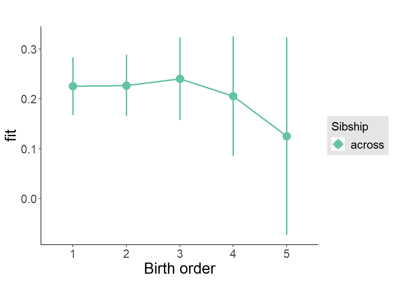
Add Interaction
Model Summary
m4_interaction = update(m3_birthorder_nonlinear, formula = . ~ . - birth_order_nonlinear - sibling_count + count_birth_order)
tidy(m4_interaction, conf.int = T, conf.level = 0.995)| effect | group | term | estimate | std.error | statistic | df | p.value | conf.low | conf.high |
|---|---|---|---|---|---|---|---|---|---|
| fixed | NA | (Intercept) | -3.195 | 0.2044 | -15.63 | 6452 | 4.265e-54 | -3.769 | -2.621 |
| fixed | NA | poly(age, 3, raw = TRUE)1 | 0.4837 | 0.04254 | 11.37 | 6342 | 1.155e-29 | 0.3643 | 0.6031 |
| fixed | NA | poly(age, 3, raw = TRUE)2 | -0.02094 | 0.00275 | -7.614 | 6355 | 3.038e-14 | -0.02866 | -0.01322 |
| fixed | NA | poly(age, 3, raw = TRUE)3 | 0.0002943 | 0.00005514 | 5.336 | 6393 | 0.00000009803 | 0.0001395 | 0.000449 |
| fixed | NA | male | 0.03408 | 0.02032 | 1.678 | 6977 | 0.09346 | -0.02295 | 0.09111 |
| fixed | NA | count_birth_order2/2 | 0.005046 | 0.03211 | 0.1571 | 5808 | 0.8751 | -0.08509 | 0.09518 |
| fixed | NA | count_birth_order1/3 | -0.07786 | 0.03788 | -2.056 | 7470 | 0.03986 | -0.1842 | 0.02847 |
| fixed | NA | count_birth_order2/3 | -0.07189 | 0.03638 | -1.976 | 7482 | 0.04821 | -0.174 | 0.03024 |
| fixed | NA | count_birth_order3/3 | -0.011 | 0.03982 | -0.2761 | 7507 | 0.7825 | -0.1228 | 0.1008 |
| fixed | NA | count_birth_order1/4 | -0.04491 | 0.0597 | -0.7523 | 7375 | 0.4519 | -0.2125 | 0.1227 |
| fixed | NA | count_birth_order2/4 | -0.09627 | 0.05238 | -1.838 | 7489 | 0.06612 | -0.2433 | 0.05077 |
| fixed | NA | count_birth_order3/4 | -0.187 | 0.04996 | -3.743 | 7489 | 0.0001831 | -0.3273 | -0.04677 |
| fixed | NA | count_birth_order4/4 | -0.1058 | 0.04949 | -2.137 | 7510 | 0.03261 | -0.2447 | 0.03315 |
| fixed | NA | count_birth_order1/5 | -0.1948 | 0.1038 | -1.877 | 6429 | 0.0606 | -0.4861 | 0.09655 |
| fixed | NA | count_birth_order2/5 | -0.1427 | 0.09249 | -1.543 | 6810 | 0.1228 | -0.4024 | 0.1169 |
| fixed | NA | count_birth_order3/5 | -0.08111 | 0.07832 | -1.036 | 7206 | 0.3004 | -0.301 | 0.1387 |
| fixed | NA | count_birth_order4/5 | -0.2496 | 0.06489 | -3.846 | 7495 | 0.0001211 | -0.4317 | -0.06741 |
| fixed | NA | count_birth_order5/5 | -0.2774 | 0.06294 | -4.407 | 7510 | 0.00001064 | -0.4541 | -0.1007 |
| ran_pars | mother_pidlink | sd__(Intercept) | 0.498 | NA | NA | NA | NA | NA | NA |
| ran_pars | Residual | sd__Observation | 0.7631 | NA | NA | NA | NA | NA | NA |
Coefficient Plot
plot_birthorder(m4_interaction)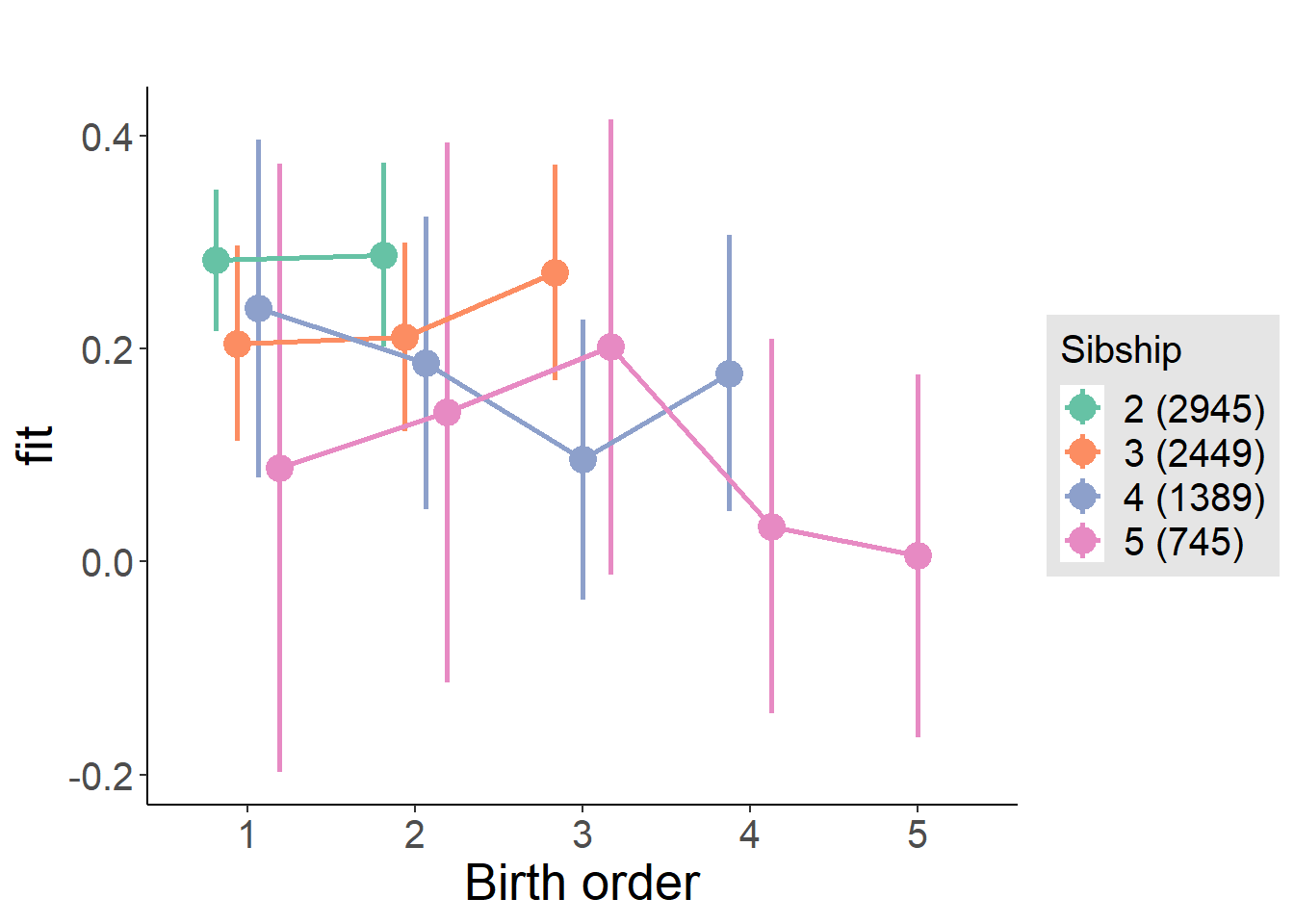
Model Comparison
###### Model 1 - Model 2
anova(m1_covariates_only, m2_birthorder_linear, m3_birthorder_nonlinear, m4_interaction)
## refitting model(s) with ML (instead of REML)| Df | AIC | BIC | logLik | deviance | Chisq | Chi Df | Pr(>Chisq) |
|---|---|---|---|---|---|---|---|
| 10 | 19714 | 19783 | -9847 | 19694 | NA | NA | NA |
| 11 | 19715 | 19792 | -9847 | 19693 | 0.2484 | 1 | 0.6182 |
| 14 | 19719 | 19816 | -9846 | 19691 | 2.358 | 3 | 0.5015 |
| 20 | 19720 | 19858 | -9840 | 19680 | 11.06 | 6 | 0.08663 |
Maternal pregnancy order
outcome_preg_m1 <- update(m2_birthorder_linear, data = birthorder %>%
  mutate(sibling_count = sibling_count_uterus_preg_factor,
         birth_order_nonlinear = birthorder_uterus_preg_factor,
         birth_order = birthorder_uterus_preg,
         count_birth_order = count_birthorder_uterus_preg
         ) %>%
    filter(sibling_count != "1"))
compare_models_markdown(outcome_preg_m1)
Basic Model
Model Summary
m1_covariates_only <- update(m2_birthorder_linear, formula = . ~ . - birth_order)
tidy(m1_covariates_only, conf.int = T, conf.level = 0.995)| effect | group | term | estimate | std.error | statistic | df | p.value | conf.low | conf.high |
|---|---|---|---|---|---|---|---|---|---|
| fixed | NA | (Intercept) | -3.236 | 0.207 | -15.63 | 5981 | 5.156e-54 | -3.817 | -2.655 |
| fixed | NA | poly(age, 3, raw = TRUE)1 | 0.4936 | 0.04358 | 11.33 | 5963 | 1.942e-29 | 0.3713 | 0.6159 |
| fixed | NA | poly(age, 3, raw = TRUE)2 | -0.02181 | 0.002828 | -7.711 | 6002 | 1.455e-14 | -0.02975 | -0.01387 |
| fixed | NA | poly(age, 3, raw = TRUE)3 | 0.000314 | 0.00005687 | 5.521 | 6038 | 0.00000003512 | 0.0001543 | 0.0004736 |
| fixed | NA | male | 0.0372 | 0.02081 | 1.788 | 6607 | 0.07384 | -0.02121 | 0.09561 |
| fixed | NA | sibling_count3 | -0.04103 | 0.02859 | -1.435 | 4602 | 0.1513 | -0.1213 | 0.03922 |
| fixed | NA | sibling_count4 | -0.07103 | 0.03369 | -2.109 | 4157 | 0.03504 | -0.1656 | 0.02353 |
| fixed | NA | sibling_count5 | -0.08426 | 0.03954 | -2.131 | 3839 | 0.03315 | -0.1953 | 0.02673 |
| ran_pars | mother_pidlink | sd__(Intercept) | 0.5057 | NA | NA | NA | NA | NA | NA |
| ran_pars | Residual | sd__Observation | 0.76 | NA | NA | NA | NA | NA | NA |
Coefficient Plot
plot(allEffects(m1_covariates_only, confidence.level = 0.995))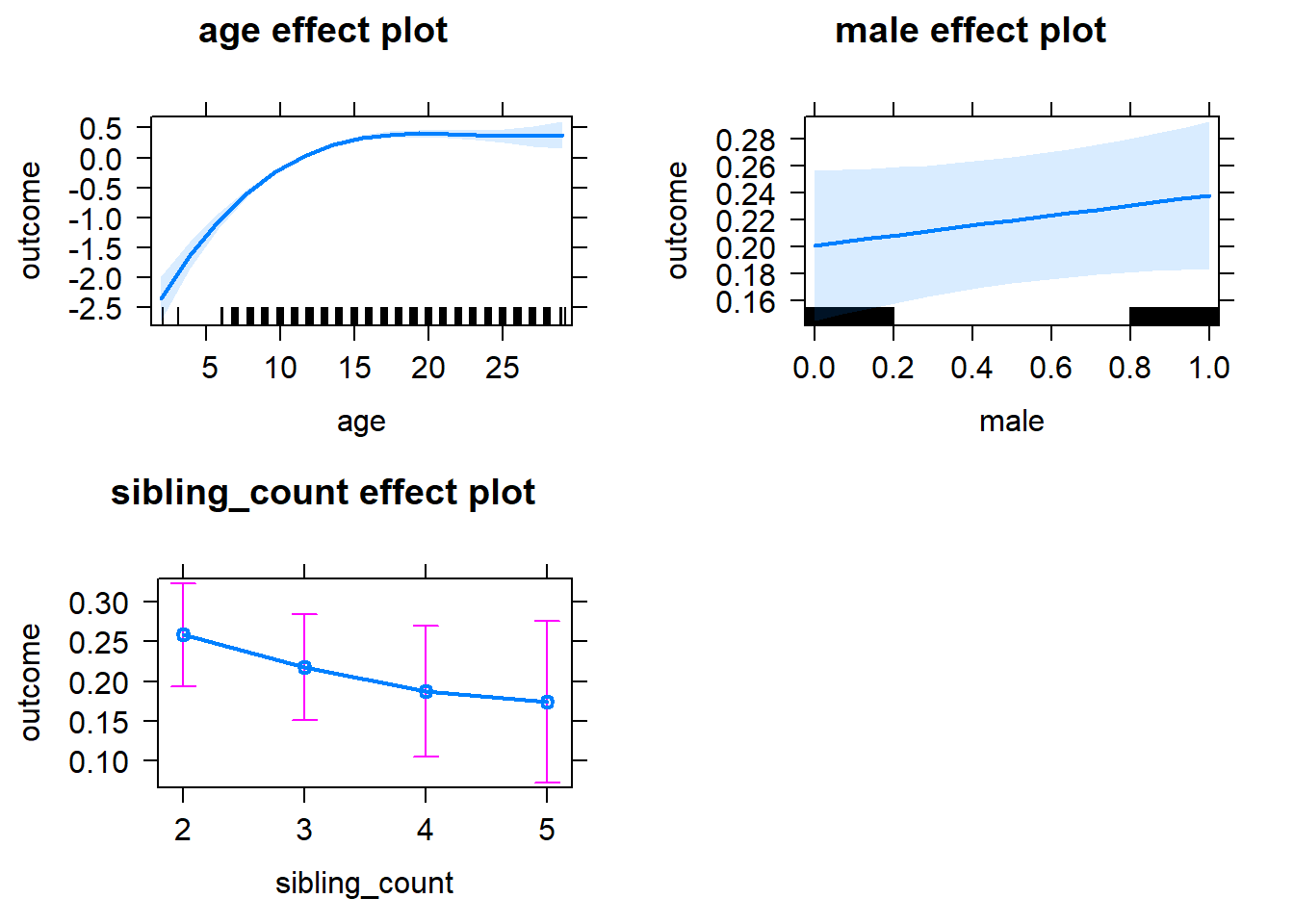
Add Birth Order Linear
Model Summary
tidy(m2_birthorder_linear, conf.int = T, conf.level = 0.995)| effect | group | term | estimate | std.error | statistic | df | p.value | conf.low | conf.high |
|---|---|---|---|---|---|---|---|---|---|
| fixed | NA | (Intercept) | -3.183 | 0.2099 | -15.16 | 6126 | 5.295e-51 | -3.772 | -2.594 |
| fixed | NA | birth_order | -0.01834 | 0.01212 | -1.513 | 6902 | 0.1302 | -0.05235 | 0.01567 |
| fixed | NA | poly(age, 3, raw = TRUE)1 | 0.4896 | 0.04366 | 11.21 | 5984 | 6.801e-29 | 0.367 | 0.6121 |
| fixed | NA | poly(age, 3, raw = TRUE)2 | -0.02165 | 0.00283 | -7.649 | 6002 | 2.349e-14 | -0.02959 | -0.0137 |
| fixed | NA | poly(age, 3, raw = TRUE)3 | 0.0003117 | 0.00005689 | 5.478 | 6036 | 0.00000004464 | 0.000152 | 0.0004714 |
| fixed | NA | male | 0.03765 | 0.02081 | 1.809 | 6610 | 0.07044 | -0.02076 | 0.09606 |
| fixed | NA | sibling_count3 | -0.0296 | 0.02956 | -1.001 | 4714 | 0.3168 | -0.1126 | 0.05338 |
| fixed | NA | sibling_count4 | -0.0452 | 0.03775 | -1.197 | 4574 | 0.2313 | -0.1512 | 0.06078 |
| fixed | NA | sibling_count5 | -0.04361 | 0.04778 | -0.9126 | 4631 | 0.3615 | -0.1777 | 0.09052 |
| ran_pars | mother_pidlink | sd__(Intercept) | 0.5051 | NA | NA | NA | NA | NA | NA |
| ran_pars | Residual | sd__Observation | 0.7602 | NA | NA | NA | NA | NA | NA |
Coefficient Plot
plot_birthorder2(m2_birthorder_linear, separate = FALSE)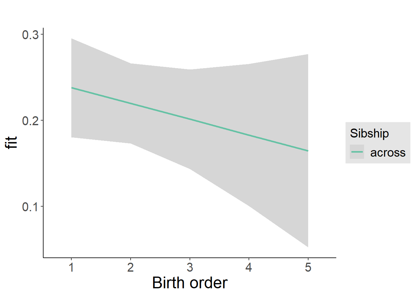
Add Birth Order Factor
Model Summary
m3_birthorder_nonlinear = update(m1_covariates_only, formula = . ~ . + birth_order_nonlinear)
tidy(m3_birthorder_nonlinear, conf.int = T, conf.level = 0.995)| effect | group | term | estimate | std.error | statistic | df | p.value | conf.low | conf.high |
|---|---|---|---|---|---|---|---|---|---|
| fixed | NA | (Intercept) | -3.207 | 0.2087 | -15.37 | 6086 | 2.571e-52 | -3.793 | -2.622 |
| fixed | NA | poly(age, 3, raw = TRUE)1 | 0.4899 | 0.04368 | 11.22 | 5989 | 6.65e-29 | 0.3673 | 0.6125 |
| fixed | NA | poly(age, 3, raw = TRUE)2 | -0.02164 | 0.002831 | -7.644 | 6005 | 2.433e-14 | -0.02959 | -0.0137 |
| fixed | NA | poly(age, 3, raw = TRUE)3 | 0.0003113 | 0.00005692 | 5.468 | 6038 | 0.00000004722 | 0.0001515 | 0.000471 |
| fixed | NA | male | 0.03721 | 0.02081 | 1.788 | 6609 | 0.07384 | -0.02121 | 0.09564 |
| fixed | NA | sibling_count3 | -0.03506 | 0.03023 | -1.16 | 4976 | 0.2462 | -0.1199 | 0.0498 |
| fixed | NA | sibling_count4 | -0.05354 | 0.03867 | -1.385 | 4802 | 0.1662 | -0.1621 | 0.055 |
| fixed | NA | sibling_count5 | -0.03095 | 0.04906 | -0.6308 | 4777 | 0.5282 | -0.1687 | 0.1068 |
| fixed | NA | birth_order_nonlinear2 | -0.01075 | 0.02398 | -0.4481 | 5054 | 0.6541 | -0.07806 | 0.05657 |
| fixed | NA | birth_order_nonlinear3 | -0.01769 | 0.03288 | -0.538 | 6027 | 0.5906 | -0.11 | 0.07461 |
| fixed | NA | birth_order_nonlinear4 | -0.04186 | 0.04566 | -0.9167 | 6379 | 0.3593 | -0.17 | 0.08632 |
| fixed | NA | birth_order_nonlinear5 | -0.1356 | 0.06807 | -1.991 | 6336 | 0.04647 | -0.3266 | 0.05552 |
| ran_pars | mother_pidlink | sd__(Intercept) | 0.5049 | NA | NA | NA | NA | NA | NA |
| ran_pars | Residual | sd__Observation | 0.7604 | NA | NA | NA | NA | NA | NA |
Coefficient Plot
plot_birthorder(m3_birthorder_nonlinear, separate = FALSE)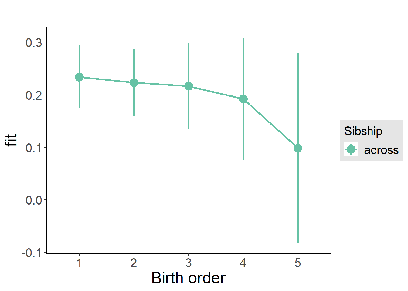
Add Interaction
Model Summary
m4_interaction = update(m3_birthorder_nonlinear, formula = . ~ . - birth_order_nonlinear - sibling_count + count_birth_order)
tidy(m4_interaction, conf.int = T, conf.level = 0.995)| effect | group | term | estimate | std.error | statistic | df | p.value | conf.low | conf.high |
|---|---|---|---|---|---|---|---|---|---|
| fixed | NA | (Intercept) | -3.22 | 0.2096 | -15.36 | 6100 | 2.669e-52 | -3.808 | -2.631 |
| fixed | NA | poly(age, 3, raw = TRUE)1 | 0.4937 | 0.04374 | 11.29 | 5994 | 3.06e-29 | 0.3709 | 0.6164 |
| fixed | NA | poly(age, 3, raw = TRUE)2 | -0.02193 | 0.002835 | -7.734 | 6003 | 1.211e-14 | -0.02989 | -0.01397 |
| fixed | NA | poly(age, 3, raw = TRUE)3 | 0.0003176 | 0.00005699 | 5.573 | 6033 | 0.00000002611 | 0.0001577 | 0.0004776 |
| fixed | NA | male | 0.03796 | 0.02082 | 1.824 | 6597 | 0.06827 | -0.02047 | 0.09639 |
| fixed | NA | count_birth_order2/2 | -0.01805 | 0.03503 | -0.5153 | 5430 | 0.6063 | -0.1164 | 0.08028 |
| fixed | NA | count_birth_order1/3 | -0.06167 | 0.03921 | -1.573 | 7122 | 0.1158 | -0.1717 | 0.0484 |
| fixed | NA | count_birth_order2/3 | -0.05229 | 0.0383 | -1.365 | 7136 | 0.1722 | -0.1598 | 0.05522 |
| fixed | NA | count_birth_order3/3 | -0.02024 | 0.04198 | -0.4821 | 7150 | 0.6297 | -0.1381 | 0.09761 |
| fixed | NA | count_birth_order1/4 | -0.052 | 0.05836 | -0.891 | 7062 | 0.373 | -0.2158 | 0.1118 |
| fixed | NA | count_birth_order2/4 | -0.05039 | 0.05238 | -0.962 | 7116 | 0.3361 | -0.1974 | 0.09663 |
| fixed | NA | count_birth_order3/4 | -0.1357 | 0.0501 | -2.709 | 7127 | 0.006758 | -0.2764 | 0.004895 |
| fixed | NA | count_birth_order4/4 | -0.05579 | 0.05067 | -1.101 | 7152 | 0.2709 | -0.198 | 0.08643 |
| fixed | NA | count_birth_order1/5 | 0.08461 | 0.08474 | 0.9984 | 6510 | 0.3181 | -0.1533 | 0.3225 |
| fixed | NA | count_birth_order2/5 | -0.03531 | 0.07586 | -0.4655 | 6802 | 0.6416 | -0.2482 | 0.1776 |
| fixed | NA | count_birth_order3/5 | -0.03455 | 0.06811 | -0.5073 | 6948 | 0.612 | -0.2257 | 0.1566 |
| fixed | NA | count_birth_order4/5 | -0.1467 | 0.06276 | -2.338 | 7056 | 0.01942 | -0.3229 | 0.02944 |
| fixed | NA | count_birth_order5/5 | -0.1714 | 0.06045 | -2.835 | 7143 | 0.004597 | -0.341 | -0.001684 |
| ran_pars | mother_pidlink | sd__(Intercept) | 0.5055 | NA | NA | NA | NA | NA | NA |
| ran_pars | Residual | sd__Observation | 0.7599 | NA | NA | NA | NA | NA | NA |
Coefficient Plot
plot_birthorder(m4_interaction)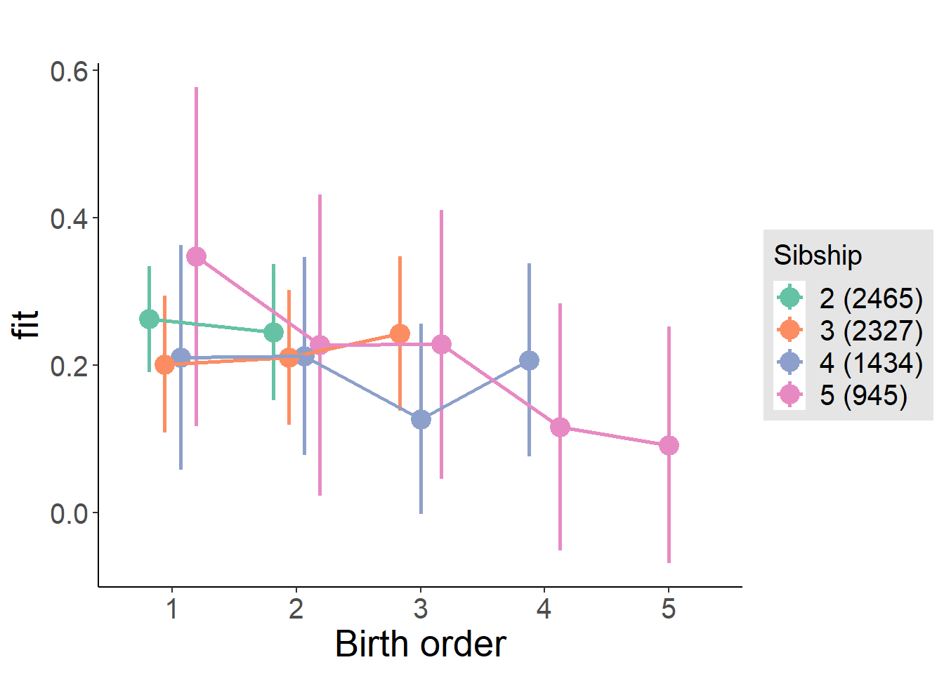
Model Comparison
###### Model 1 - Model 2
anova(m1_covariates_only, m2_birthorder_linear, m3_birthorder_nonlinear, m4_interaction)
## refitting model(s) with ML (instead of REML)| Df | AIC | BIC | logLik | deviance | Chisq | Chi Df | Pr(>Chisq) |
|---|---|---|---|---|---|---|---|
| 10 | 18797 | 18866 | -9389 | 18777 | NA | NA | NA |
| 11 | 18797 | 18872 | -9387 | 18775 | 2.293 | 1 | 0.1299 |
| 14 | 18801 | 18897 | -9386 | 18773 | 1.75 | 3 | 0.6258 |
| 20 | 18804 | 18941 | -9382 | 18764 | 9.378 | 6 | 0.1534 |
Parental full sibling order
outcome_parental_m1 <- update(m2_birthorder_linear, data = birthorder %>%
  mutate(sibling_count = sibling_count_genes_factor,
         birth_order_nonlinear = birthorder_genes_factor,
         birth_order = birthorder_genes,
         count_birth_order = count_birthorder_genes
         ) %>%
      filter(sibling_count != "1"))
compare_models_markdown(outcome_parental_m1)
Basic Model
Model Summary
m1_covariates_only <- update(m2_birthorder_linear, formula = . ~ . - birth_order)
tidy(m1_covariates_only, conf.int = T, conf.level = 0.995)| effect | group | term | estimate | std.error | statistic | df | p.value | conf.low | conf.high |
|---|---|---|---|---|---|---|---|---|---|
| fixed | NA | (Intercept) | -3.181 | 0.2033 | -15.65 | 6211 | 3.641e-54 | -3.751 | -2.61 |
| fixed | NA | poly(age, 3, raw = TRUE)1 | 0.4799 | 0.04263 | 11.26 | 6214 | 4.035e-29 | 0.3603 | 0.5996 |
| fixed | NA | poly(age, 3, raw = TRUE)2 | -0.0207 | 0.002756 | -7.508 | 6268 | 6.824e-14 | -0.02843 | -0.01296 |
| fixed | NA | poly(age, 3, raw = TRUE)3 | 0.0002895 | 0.00005525 | 5.241 | 6320 | 0.0000001652 | 0.0001345 | 0.0004446 |
| fixed | NA | male | 0.02833 | 0.02045 | 1.385 | 6861 | 0.166 | -0.02907 | 0.08573 |
| fixed | NA | sibling_count3 | -0.0465 | 0.02731 | -1.703 | 4573 | 0.08869 | -0.1232 | 0.03016 |
| fixed | NA | sibling_count4 | -0.09864 | 0.03383 | -2.915 | 3966 | 0.003572 | -0.1936 | -0.003666 |
| fixed | NA | sibling_count5 | -0.2016 | 0.04479 | -4.502 | 3600 | 0.000006955 | -0.3273 | -0.0759 |
| ran_pars | mother_pidlink | sd__(Intercept) | 0.4979 | NA | NA | NA | NA | NA | NA |
| ran_pars | Residual | sd__Observation | 0.7613 | NA | NA | NA | NA | NA | NA |
Coefficient Plot
plot(allEffects(m1_covariates_only, confidence.level = 0.995))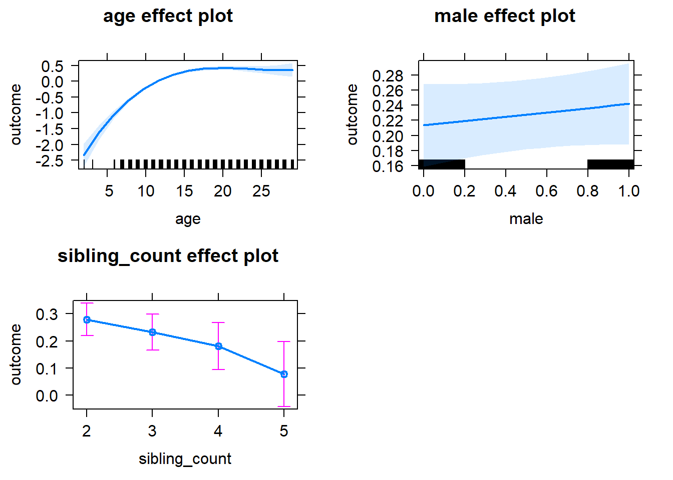
Add Birth Order Linear
Model Summary
tidy(m2_birthorder_linear, conf.int = T, conf.level = 0.995)| effect | group | term | estimate | std.error | statistic | df | p.value | conf.low | conf.high |
|---|---|---|---|---|---|---|---|---|---|
| fixed | NA | (Intercept) | -3.164 | 0.2065 | -15.32 | 6375 | 4.637e-52 | -3.743 | -2.584 |
| fixed | NA | birth_order | -0.005982 | 0.01263 | -0.4735 | 7010 | 0.6359 | -0.04145 | 0.02948 |
| fixed | NA | poly(age, 3, raw = TRUE)1 | 0.4786 | 0.04272 | 11.21 | 6239 | 7.226e-29 | 0.3587 | 0.5986 |
| fixed | NA | poly(age, 3, raw = TRUE)2 | -0.02065 | 0.002759 | -7.485 | 6268 | 8.133e-14 | -0.02839 | -0.0129 |
| fixed | NA | poly(age, 3, raw = TRUE)3 | 0.0002889 | 0.00005527 | 5.227 | 6317 | 0.0000001777 | 0.0001338 | 0.000444 |
| fixed | NA | male | 0.02843 | 0.02045 | 1.39 | 6862 | 0.1645 | -0.02898 | 0.08584 |
| fixed | NA | sibling_count3 | -0.04256 | 0.02855 | -1.491 | 4691 | 0.1361 | -0.1227 | 0.03758 |
| fixed | NA | sibling_count4 | -0.08986 | 0.03859 | -2.329 | 4438 | 0.01992 | -0.1982 | 0.01845 |
| fixed | NA | sibling_count5 | -0.1872 | 0.05414 | -3.458 | 4433 | 0.0005493 | -0.3392 | -0.03524 |
| ran_pars | mother_pidlink | sd__(Intercept) | 0.4978 | NA | NA | NA | NA | NA | NA |
| ran_pars | Residual | sd__Observation | 0.7614 | NA | NA | NA | NA | NA | NA |
Coefficient Plot
plot_birthorder2(m2_birthorder_linear, separate = FALSE)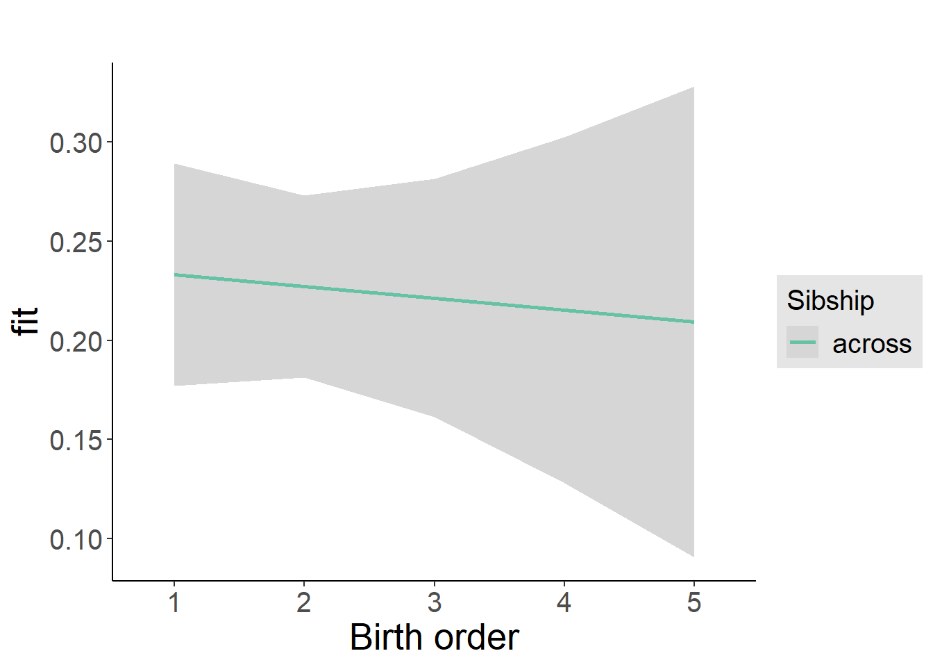
Add Birth Order Factor
Model Summary
m3_birthorder_nonlinear = update(m1_covariates_only, formula = . ~ . + birth_order_nonlinear)
tidy(m3_birthorder_nonlinear, conf.int = T, conf.level = 0.995)| effect | group | term | estimate | std.error | statistic | df | p.value | conf.low | conf.high |
|---|---|---|---|---|---|---|---|---|---|
| fixed | NA | (Intercept) | -3.174 | 0.205 | -15.48 | 6330 | 4.172e-53 | -3.75 | -2.599 |
| fixed | NA | poly(age, 3, raw = TRUE)1 | 0.4787 | 0.04273 | 11.2 | 6244 | 7.443e-29 | 0.3588 | 0.5987 |
| fixed | NA | poly(age, 3, raw = TRUE)2 | -0.02064 | 0.002759 | -7.478 | 6271 | 8.577e-14 | -0.02838 | -0.01289 |
| fixed | NA | poly(age, 3, raw = TRUE)3 | 0.0002884 | 0.00005529 | 5.216 | 6319 | 0.0000001887 | 0.0001332 | 0.0004436 |
| fixed | NA | male | 0.02822 | 0.02046 | 1.379 | 6861 | 0.1679 | -0.02921 | 0.08565 |
| fixed | NA | sibling_count3 | -0.0454 | 0.02923 | -1.553 | 4980 | 0.1204 | -0.1275 | 0.03665 |
| fixed | NA | sibling_count4 | -0.09354 | 0.03953 | -2.366 | 4679 | 0.01802 | -0.2045 | 0.01743 |
| fixed | NA | sibling_count5 | -0.1703 | 0.05714 | -2.98 | 4668 | 0.002896 | -0.3307 | -0.009892 |
| fixed | NA | birth_order_nonlinear2 | 0.003025 | 0.02311 | 0.1309 | 5256 | 0.8959 | -0.06184 | 0.06789 |
| fixed | NA | birth_order_nonlinear3 | -0.002564 | 0.03312 | -0.07743 | 6087 | 0.9383 | -0.09553 | 0.09041 |
| fixed | NA | birth_order_nonlinear4 | -0.01117 | 0.04779 | -0.2337 | 6424 | 0.8152 | -0.1453 | 0.123 |
| fixed | NA | birth_order_nonlinear5 | -0.07969 | 0.07807 | -1.021 | 6509 | 0.3074 | -0.2988 | 0.1395 |
| ran_pars | mother_pidlink | sd__(Intercept) | 0.4975 | NA | NA | NA | NA | NA | NA |
| ran_pars | Residual | sd__Observation | 0.7617 | NA | NA | NA | NA | NA | NA |
Coefficient Plot
plot_birthorder(m3_birthorder_nonlinear, separate = FALSE)
Add Interaction
Model Summary
m4_interaction = update(m3_birthorder_nonlinear, formula = . ~ . - birth_order_nonlinear - sibling_count + count_birth_order)
tidy(m4_interaction, conf.int = T, conf.level = 0.995)| effect | group | term | estimate | std.error | statistic | df | p.value | conf.low | conf.high |
|---|---|---|---|---|---|---|---|---|---|
| fixed | NA | (Intercept) | -3.174 | 0.2056 | -15.44 | 6344 | 7.73e-53 | -3.751 | -2.597 |
| fixed | NA | poly(age, 3, raw = TRUE)1 | 0.479 | 0.04277 | 11.2 | 6245 | 7.531e-29 | 0.359 | 0.5991 |
| fixed | NA | poly(age, 3, raw = TRUE)2 | -0.02067 | 0.002762 | -7.485 | 6265 | 8.126e-14 | -0.02842 | -0.01292 |
| fixed | NA | poly(age, 3, raw = TRUE)3 | 0.0002893 | 0.00005533 | 5.229 | 6309 | 0.0000001757 | 0.000134 | 0.0004446 |
| fixed | NA | male | 0.02905 | 0.02046 | 1.42 | 6848 | 0.1556 | -0.02837 | 0.08647 |
| fixed | NA | count_birth_order2/2 | 0.0009753 | 0.03179 | 0.03068 | 5649 | 0.9755 | -0.08825 | 0.0902 |
| fixed | NA | count_birth_order1/3 | -0.06278 | 0.03805 | -1.65 | 7333 | 0.09903 | -0.1696 | 0.04404 |
| fixed | NA | count_birth_order2/3 | -0.05251 | 0.0365 | -1.439 | 7343 | 0.1503 | -0.155 | 0.04994 |
| fixed | NA | count_birth_order3/3 | -0.0171 | 0.04001 | -0.4274 | 7369 | 0.6691 | -0.1294 | 0.0952 |
| fixed | NA | count_birth_order1/4 | -0.04273 | 0.06007 | -0.7113 | 7251 | 0.4769 | -0.2113 | 0.1259 |
| fixed | NA | count_birth_order2/4 | -0.07004 | 0.05307 | -1.32 | 7347 | 0.187 | -0.219 | 0.07894 |
| fixed | NA | count_birth_order3/4 | -0.1841 | 0.05035 | -3.656 | 7352 | 0.000258 | -0.3254 | -0.04274 |
| fixed | NA | count_birth_order4/4 | -0.07312 | 0.05019 | -1.457 | 7370 | 0.1452 | -0.214 | 0.06777 |
| fixed | NA | count_birth_order1/5 | -0.1874 | 0.1038 | -1.806 | 6471 | 0.07096 | -0.4786 | 0.1039 |
| fixed | NA | count_birth_order2/5 | -0.1367 | 0.09923 | -1.377 | 6587 | 0.1685 | -0.4152 | 0.1419 |
| fixed | NA | count_birth_order3/5 | -0.07523 | 0.08045 | -0.9351 | 7132 | 0.3498 | -0.3011 | 0.1506 |
| fixed | NA | count_birth_order4/5 | -0.2492 | 0.06826 | -3.651 | 7352 | 0.0002628 | -0.4409 | -0.05763 |
| fixed | NA | count_birth_order5/5 | -0.2523 | 0.06671 | -3.783 | 7370 | 0.0001564 | -0.4396 | -0.06508 |
| ran_pars | mother_pidlink | sd__(Intercept) | 0.4979 | NA | NA | NA | NA | NA | NA |
| ran_pars | Residual | sd__Observation | 0.7611 | NA | NA | NA | NA | NA | NA |
Coefficient Plot
plot_birthorder(m4_interaction)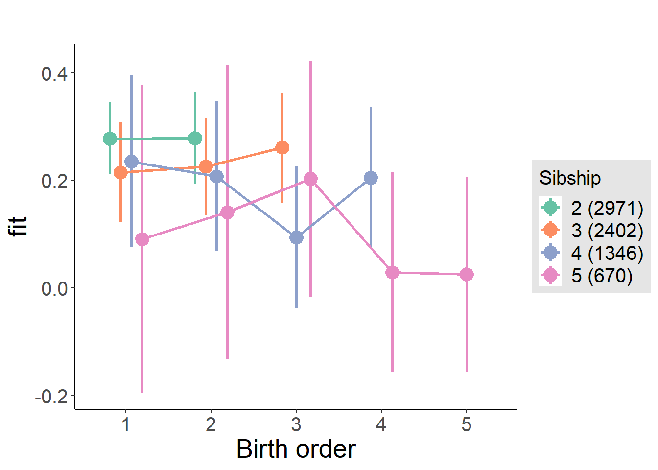
Model Comparison
###### Model 1 - Model 2
anova(m1_covariates_only, m2_birthorder_linear, m3_birthorder_nonlinear, m4_interaction)
## refitting model(s) with ML (instead of REML)| Df | AIC | BIC | logLik | deviance | Chisq | Chi Df | Pr(>Chisq) |
|---|---|---|---|---|---|---|---|
| 10 | 19316 | 19385 | -9648 | 19296 | NA | NA | NA |
| 11 | 19318 | 19394 | -9648 | 19296 | 0.2247 | 1 | 0.6355 |
| 14 | 19323 | 19420 | -9647 | 19295 | 0.9323 | 3 | 0.8176 |
| 20 | 19324 | 19462 | -9642 | 19284 | 10.87 | 6 | 0.09248 |
Compare birth order specifications
library(coefplot)
multiplot(outcome_naive_m1, outcome_preg_m1, outcome_uterus_m1, outcome_parental_m1, dodgeHeight = 0.6,
          intercept = FALSE)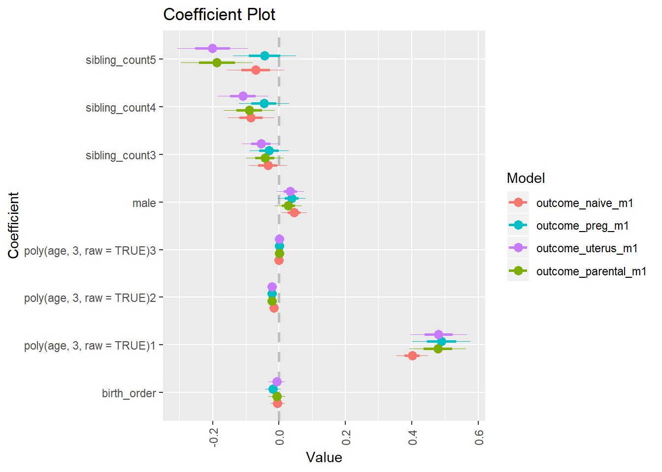
Numeracy 2015 young
birthorder <- birthorder %>% mutate(outcome = math_2015_young)
model = lmer(outcome ~ birth_order + poly(age, 3, raw = TRUE) + male + sibling_count + (1 | mother_pidlink),
                   data = birthorder)
compare_birthorder_specs(model)
Naive birth order
outcome_naive_m1 <- update(m2_birthorder_linear, data = birthorder %>%
                     mutate(sibling_count = sibling_count_naive_factor,
                            birth_order_nonlinear = birthorder_naive_factor,
                            birth_order = birthorder_naive,
                            count_birth_order = count_birthorder_naive) %>%
                     filter(sibling_count != "1"))
compare_models_markdown(outcome_naive_m1)
Basic Model
Model Summary
m1_covariates_only <- update(m2_birthorder_linear, formula = . ~ . - birth_order)
tidy(m1_covariates_only, conf.int = T, conf.level = 0.995)| effect | group | term | estimate | std.error | statistic | df | p.value | conf.low | conf.high |
|---|---|---|---|---|---|---|---|---|---|
| fixed | NA | (Intercept) | -2.4 | 0.1332 | -18.01 | 7928 | 3.943e-71 | -2.774 | -2.026 |
| fixed | NA | poly(age, 3, raw = TRUE)1 | 0.3891 | 0.02467 | 15.77 | 8038 | 3.269e-55 | 0.3198 | 0.4583 |
| fixed | NA | poly(age, 3, raw = TRUE)2 | -0.01698 | 0.001415 | -12 | 8129 | 6.933e-33 | -0.02095 | -0.01301 |
| fixed | NA | poly(age, 3, raw = TRUE)3 | 0.0002247 | 0.00002571 | 8.739 | 8114 | 2.817e-18 | 0.0001525 | 0.0002969 |
| fixed | NA | male | -0.1652 | 0.02089 | -7.909 | 7770 | 2.954e-15 | -0.2238 | -0.1066 |
| fixed | NA | sibling_count3 | -0.003366 | 0.02911 | -0.1156 | 5422 | 0.908 | -0.08509 | 0.07836 |
| fixed | NA | sibling_count4 | -0.08741 | 0.03267 | -2.676 | 4870 | 0.007485 | -0.1791 | 0.004294 |
| fixed | NA | sibling_count5 | -0.04743 | 0.03694 | -1.284 | 4352 | 0.1991 | -0.1511 | 0.05625 |
| ran_pars | mother_pidlink | sd__(Intercept) | 0.4677 | NA | NA | NA | NA | NA | NA |
| ran_pars | Residual | sd__Observation | 0.842 | NA | NA | NA | NA | NA | NA |
Coefficient Plot
plot(allEffects(m1_covariates_only, confidence.level = 0.995))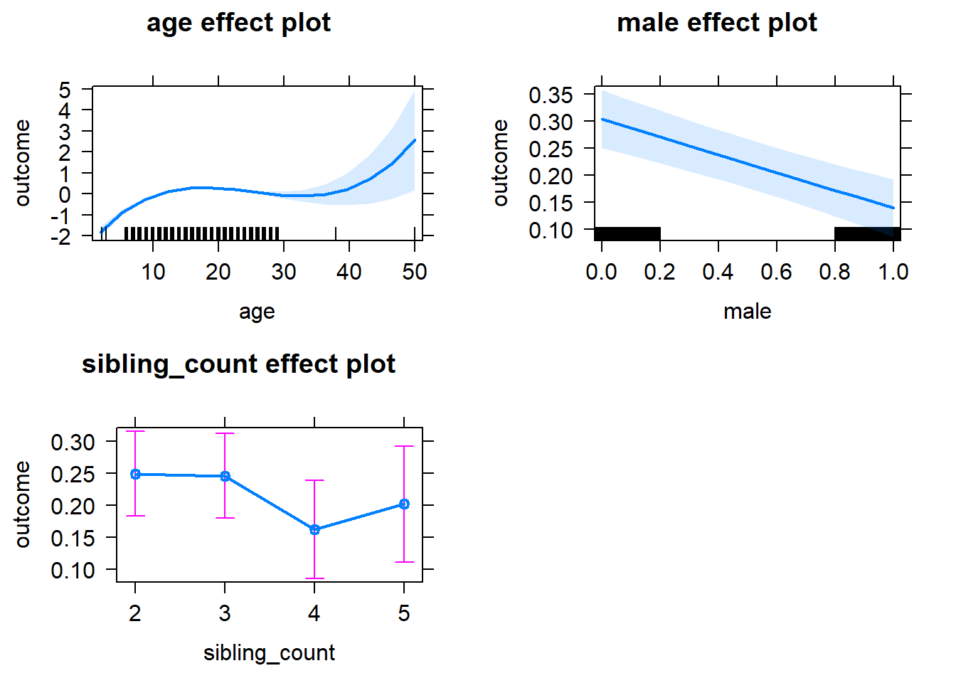
Add Birth Order Linear
Model Summary
tidy(m2_birthorder_linear, conf.int = T, conf.level = 0.995)| effect | group | term | estimate | std.error | statistic | df | p.value | conf.low | conf.high |
|---|---|---|---|---|---|---|---|---|---|
| fixed | NA | (Intercept) | -2.421 | 0.1364 | -17.75 | 8003 | 3.445e-69 | -2.804 | -2.039 |
| fixed | NA | birth_order | 0.008505 | 0.01153 | 0.7378 | 7693 | 0.4607 | -0.02386 | 0.04087 |
| fixed | NA | poly(age, 3, raw = TRUE)1 | 0.3904 | 0.02473 | 15.78 | 8043 | 2.692e-55 | 0.3209 | 0.4598 |
| fixed | NA | poly(age, 3, raw = TRUE)2 | -0.01702 | 0.001416 | -12.02 | 8127 | 5.579e-33 | -0.02099 | -0.01304 |
| fixed | NA | poly(age, 3, raw = TRUE)3 | 0.000225 | 0.00002572 | 8.751 | 8115 | 2.539e-18 | 0.0001529 | 0.0002972 |
| fixed | NA | male | -0.1653 | 0.02089 | -7.913 | 7769 | 2.852e-15 | -0.2239 | -0.1067 |
| fixed | NA | sibling_count3 | -0.008157 | 0.02983 | -0.2734 | 5545 | 0.7845 | -0.0919 | 0.07558 |
| fixed | NA | sibling_count4 | -0.09879 | 0.03613 | -2.734 | 5289 | 0.006273 | -0.2002 | 0.002629 |
| fixed | NA | sibling_count5 | -0.06581 | 0.04455 | -1.477 | 5147 | 0.1397 | -0.1909 | 0.05925 |
| ran_pars | mother_pidlink | sd__(Intercept) | 0.4678 | NA | NA | NA | NA | NA | NA |
| ran_pars | Residual | sd__Observation | 0.842 | NA | NA | NA | NA | NA | NA |
Coefficient Plot
plot_birthorder2(m2_birthorder_linear, separate = FALSE)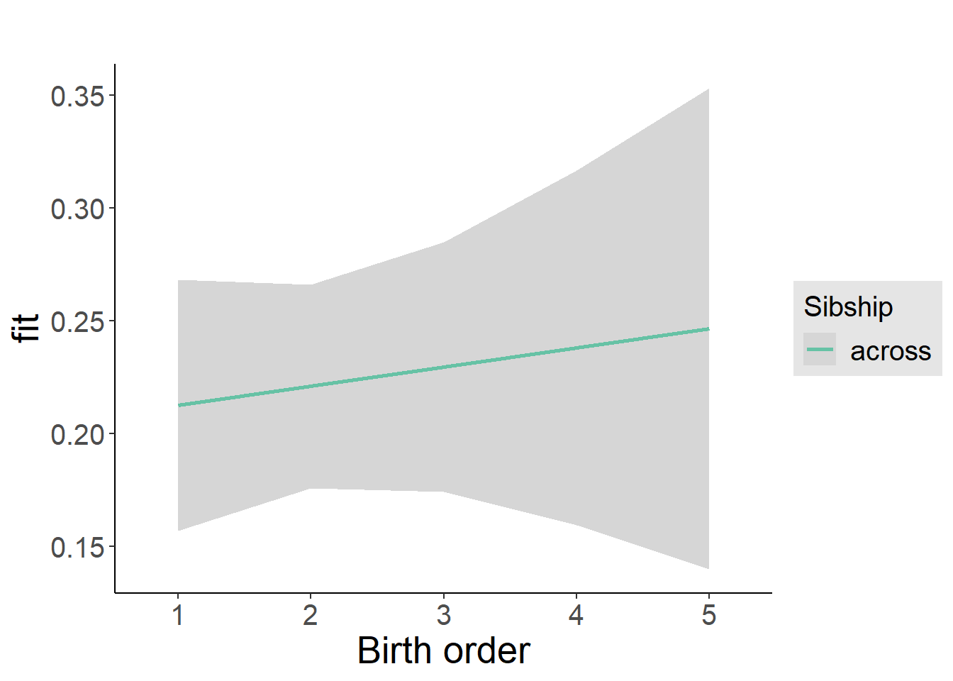
Add Birth Order Factor
Model Summary
m3_birthorder_nonlinear = update(m1_covariates_only, formula = . ~ . + birth_order_nonlinear)
tidy(m3_birthorder_nonlinear, conf.int = T, conf.level = 0.995)| effect | group | term | estimate | std.error | statistic | df | p.value | conf.low | conf.high |
|---|---|---|---|---|---|---|---|---|---|
| fixed | NA | (Intercept) | -2.421 | 0.135 | -17.94 | 7999 | 1.354e-70 | -2.8 | -2.042 |
| fixed | NA | poly(age, 3, raw = TRUE)1 | 0.391 | 0.02475 | 15.8 | 8050 | 2.125e-55 | 0.3216 | 0.4605 |
| fixed | NA | poly(age, 3, raw = TRUE)2 | -0.01705 | 0.001417 | -12.03 | 8126 | 4.687e-33 | -0.02102 | -0.01307 |
| fixed | NA | poly(age, 3, raw = TRUE)3 | 0.0002254 | 0.00002572 | 8.762 | 8110 | 2.305e-18 | 0.0001532 | 0.0002976 |
| fixed | NA | male | -0.1654 | 0.02089 | -7.918 | 7767 | 2.758e-15 | -0.224 | -0.1068 |
| fixed | NA | sibling_count3 | -0.01839 | 0.03036 | -0.6057 | 5783 | 0.5448 | -0.1036 | 0.06683 |
| fixed | NA | sibling_count4 | -0.09876 | 0.0369 | -2.676 | 5558 | 0.007466 | -0.2023 | 0.004824 |
| fixed | NA | sibling_count5 | -0.06099 | 0.04522 | -1.349 | 5253 | 0.1774 | -0.1879 | 0.06594 |
| fixed | NA | birth_order_nonlinear2 | 0.02107 | 0.02464 | 0.8551 | 6177 | 0.3925 | -0.0481 | 0.09024 |
| fixed | NA | birth_order_nonlinear3 | 0.05765 | 0.03232 | 1.784 | 6882 | 0.07448 | -0.03306 | 0.1484 |
| fixed | NA | birth_order_nonlinear4 | -0.02123 | 0.04373 | -0.4854 | 7121 | 0.6274 | -0.144 | 0.1015 |
| fixed | NA | birth_order_nonlinear5 | 0.03537 | 0.06344 | 0.5575 | 7266 | 0.5772 | -0.1427 | 0.2135 |
| ran_pars | mother_pidlink | sd__(Intercept) | 0.4678 | NA | NA | NA | NA | NA | NA |
| ran_pars | Residual | sd__Observation | 0.8419 | NA | NA | NA | NA | NA | NA |
Coefficient Plot
plot_birthorder(m3_birthorder_nonlinear, separate = FALSE)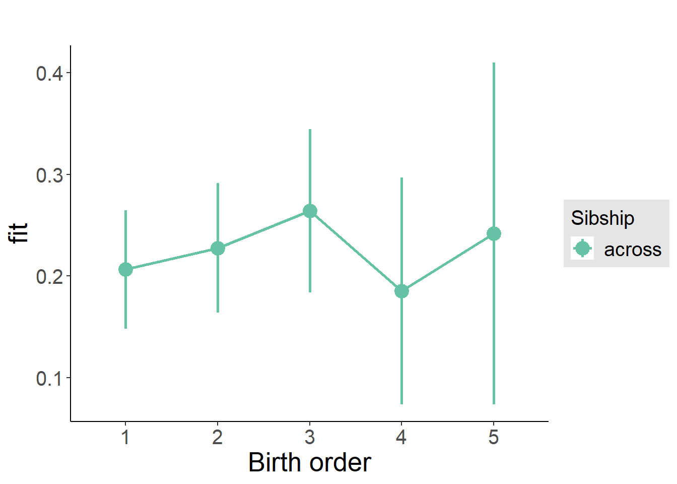
Add Interaction
Model Summary
m4_interaction = update(m3_birthorder_nonlinear, formula = . ~ . - birth_order_nonlinear - sibling_count + count_birth_order)
tidy(m4_interaction, conf.int = T, conf.level = 0.995)| effect | group | term | estimate | std.error | statistic | df | p.value | conf.low | conf.high |
|---|---|---|---|---|---|---|---|---|---|
| fixed | NA | (Intercept) | -2.43 | 0.1359 | -17.88 | 8008 | 3.81e-70 | -2.811 | -2.048 |
| fixed | NA | poly(age, 3, raw = TRUE)1 | 0.3913 | 0.02479 | 15.78 | 8052 | 2.772e-55 | 0.3217 | 0.4609 |
| fixed | NA | poly(age, 3, raw = TRUE)2 | -0.01706 | 0.001419 | -12.02 | 8120 | 5.027e-33 | -0.02105 | -0.01308 |
| fixed | NA | poly(age, 3, raw = TRUE)3 | 0.0002257 | 0.00002575 | 8.766 | 8104 | 2.231e-18 | 0.0001534 | 0.000298 |
| fixed | NA | male | -0.1654 | 0.0209 | -7.913 | 7766 | 2.867e-15 | -0.2241 | -0.1067 |
| fixed | NA | count_birth_order2/2 | 0.04371 | 0.0386 | 1.132 | 6418 | 0.2575 | -0.06464 | 0.1521 |
| fixed | NA | count_birth_order1/3 | 0.002918 | 0.03881 | 0.0752 | 8063 | 0.9401 | -0.106 | 0.1119 |
| fixed | NA | count_birth_order2/3 | 0.00944 | 0.03955 | 0.2387 | 8102 | 0.8114 | -0.1016 | 0.1205 |
| fixed | NA | count_birth_order3/3 | 0.02532 | 0.04488 | 0.5641 | 8124 | 0.5727 | -0.1007 | 0.1513 |
| fixed | NA | count_birth_order1/4 | -0.1027 | 0.05345 | -1.922 | 8120 | 0.0547 | -0.2527 | 0.04733 |
| fixed | NA | count_birth_order2/4 | -0.0895 | 0.05066 | -1.767 | 8116 | 0.07732 | -0.2317 | 0.0527 |
| fixed | NA | count_birth_order3/4 | -0.03057 | 0.04757 | -0.6427 | 8124 | 0.5205 | -0.1641 | 0.103 |
| fixed | NA | count_birth_order4/4 | -0.08469 | 0.05197 | -1.63 | 8099 | 0.1032 | -0.2306 | 0.06119 |
| fixed | NA | count_birth_order1/5 | -0.03692 | 0.07295 | -0.5061 | 7916 | 0.6128 | -0.2417 | 0.1679 |
| fixed | NA | count_birth_order2/5 | -0.04579 | 0.06922 | -0.6615 | 7954 | 0.5083 | -0.2401 | 0.1485 |
| fixed | NA | count_birth_order3/5 | 0.04616 | 0.06247 | 0.7389 | 8041 | 0.46 | -0.1292 | 0.2215 |
| fixed | NA | count_birth_order4/5 | -0.1104 | 0.05859 | -1.885 | 8091 | 0.0595 | -0.2749 | 0.05404 |
| fixed | NA | count_birth_order5/5 | -0.01793 | 0.05804 | -0.3089 | 8102 | 0.7574 | -0.1809 | 0.145 |
| ran_pars | mother_pidlink | sd__(Intercept) | 0.4669 | NA | NA | NA | NA | NA | NA |
| ran_pars | Residual | sd__Observation | 0.8425 | NA | NA | NA | NA | NA | NA |
Coefficient Plot
plot_birthorder(m4_interaction)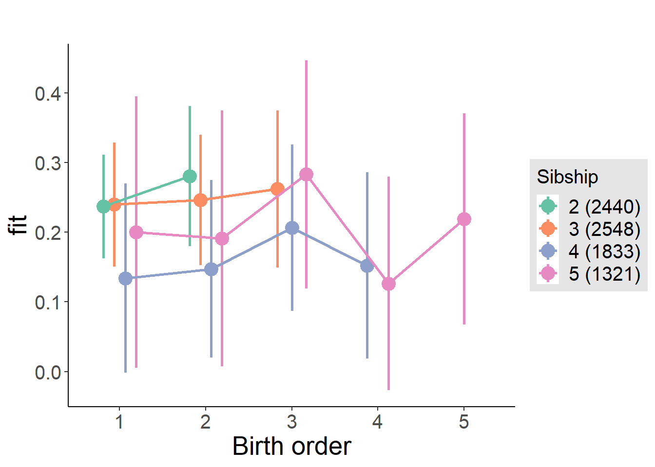
Model Comparison
###### Model 1 - Model 2
anova(m1_covariates_only, m2_birthorder_linear, m3_birthorder_nonlinear, m4_interaction)
## refitting model(s) with ML (instead of REML)| Df | AIC | BIC | logLik | deviance | Chisq | Chi Df | Pr(>Chisq) |
|---|---|---|---|---|---|---|---|
| 10 | 22322 | 22392 | -11151 | 22302 | NA | NA | NA |
| 11 | 22323 | 22400 | -11151 | 22301 | 0.5443 | 1 | 0.4607 |
| 14 | 22325 | 22423 | -11148 | 22297 | 4.614 | 3 | 0.2023 |
| 20 | 22334 | 22474 | -11147 | 22294 | 2.804 | 6 | 0.833 |
Maternal birth order
outcome_uterus_m1 <- update(m2_birthorder_linear, data = birthorder %>%
                     mutate(sibling_count = sibling_count_uterus_alive_factor,
                            birth_order_nonlinear = birthorder_uterus_alive_factor,
                            birth_order = birthorder_uterus_alive,
                            count_birth_order = count_birthorder_uterus_alive) %>%
                     filter(sibling_count != "1"))
compare_models_markdown(outcome_uterus_m1)
Basic Model
Model Summary
m1_covariates_only <- update(m2_birthorder_linear, formula = . ~ . - birth_order)
tidy(m1_covariates_only, conf.int = T, conf.level = 0.995)| effect | group | term | estimate | std.error | statistic | df | p.value | conf.low | conf.high |
|---|---|---|---|---|---|---|---|---|---|
| fixed | NA | (Intercept) | -3.178 | 0.2178 | -14.59 | 6607 | 1.729e-47 | -3.789 | -2.567 |
| fixed | NA | poly(age, 3, raw = TRUE)1 | 0.5555 | 0.04571 | 12.15 | 6610 | 1.238e-33 | 0.4272 | 0.6838 |
| fixed | NA | poly(age, 3, raw = TRUE)2 | -0.02776 | 0.002957 | -9.387 | 6654 | 8.318e-21 | -0.03606 | -0.01946 |
| fixed | NA | poly(age, 3, raw = TRUE)3 | 0.0004428 | 0.00005931 | 7.465 | 6693 | 9.354e-14 | 0.0002763 | 0.0006093 |
| fixed | NA | male | -0.1763 | 0.0218 | -8.086 | 7201 | 7.175e-16 | -0.2375 | -0.1151 |
| fixed | NA | sibling_count3 | -0.004145 | 0.0285 | -0.1454 | 4801 | 0.8844 | -0.08415 | 0.07586 |
| fixed | NA | sibling_count4 | -0.05481 | 0.03489 | -1.571 | 4121 | 0.1162 | -0.1527 | 0.04312 |
| fixed | NA | sibling_count5 | -0.1574 | 0.04468 | -3.524 | 3678 | 0.0004304 | -0.2829 | -0.03203 |
| ran_pars | mother_pidlink | sd__(Intercept) | 0.4742 | NA | NA | NA | NA | NA | NA |
| ran_pars | Residual | sd__Observation | 0.8419 | NA | NA | NA | NA | NA | NA |
Coefficient Plot
plot(allEffects(m1_covariates_only, confidence.level = 0.995))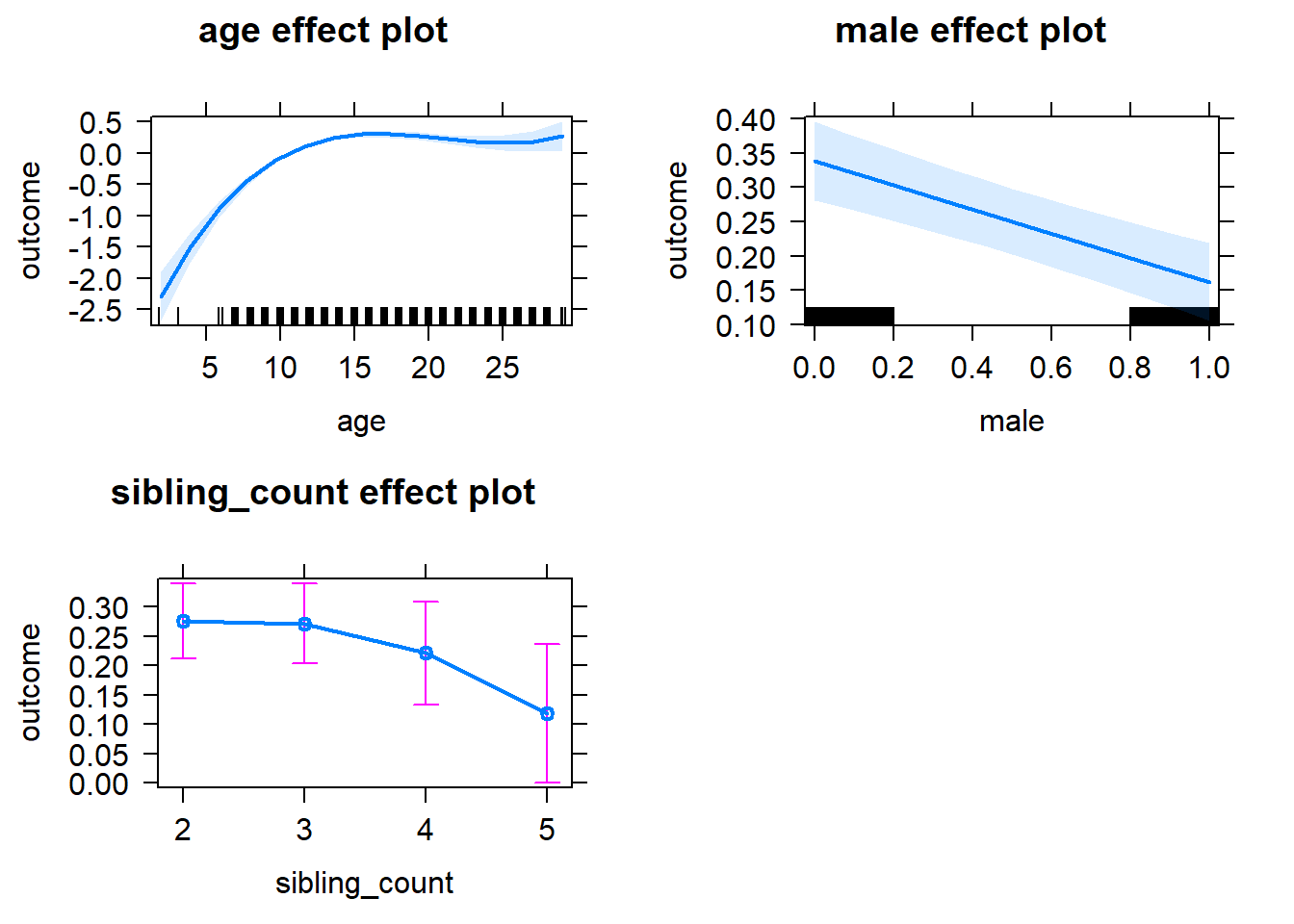
Add Birth Order Linear
Model Summary
tidy(m2_birthorder_linear, conf.int = T, conf.level = 0.995)| effect | group | term | estimate | std.error | statistic | df | p.value | conf.low | conf.high |
|---|---|---|---|---|---|---|---|---|---|
| fixed | NA | (Intercept) | -3.178 | 0.2209 | -14.38 | 6738 | 3.105e-46 | -3.798 | -2.558 |
| fixed | NA | birth_order | 0.00003101 | 0.01338 | 0.002317 | 7263 | 0.9982 | -0.03754 | 0.0376 |
| fixed | NA | poly(age, 3, raw = TRUE)1 | 0.5555 | 0.04579 | 12.13 | 6628 | 1.59e-33 | 0.427 | 0.684 |
| fixed | NA | poly(age, 3, raw = TRUE)2 | -0.02776 | 0.002959 | -9.381 | 6653 | 8.801e-21 | -0.03606 | -0.01945 |
| fixed | NA | poly(age, 3, raw = TRUE)3 | 0.0004428 | 0.00005933 | 7.463 | 6691 | 9.52e-14 | 0.0002762 | 0.0006093 |
| fixed | NA | male | -0.1763 | 0.0218 | -8.085 | 7201 | 7.23e-16 | -0.2375 | -0.1151 |
| fixed | NA | sibling_count3 | -0.004165 | 0.02981 | -0.1397 | 4910 | 0.8889 | -0.08784 | 0.07951 |
| fixed | NA | sibling_count4 | -0.05486 | 0.03995 | -1.373 | 4563 | 0.1698 | -0.167 | 0.05729 |
| fixed | NA | sibling_count5 | -0.1575 | 0.05518 | -2.855 | 4552 | 0.004328 | -0.3124 | -0.002626 |
| ran_pars | mother_pidlink | sd__(Intercept) | 0.4743 | NA | NA | NA | NA | NA | NA |
| ran_pars | Residual | sd__Observation | 0.842 | NA | NA | NA | NA | NA | NA |
Coefficient Plot
plot_birthorder2(m2_birthorder_linear, separate = FALSE)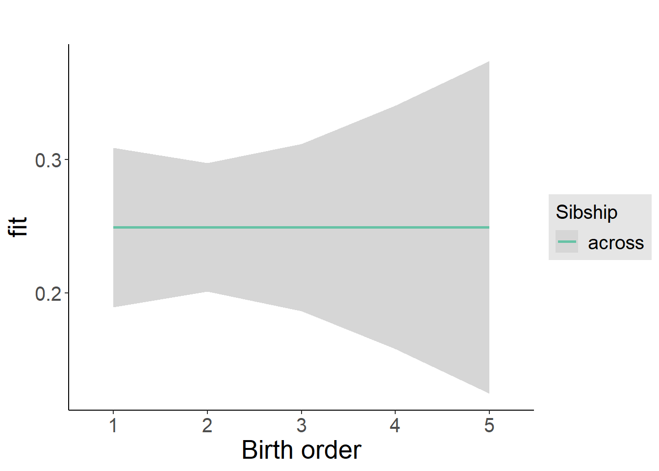
Add Birth Order Factor
Model Summary
m3_birthorder_nonlinear = update(m1_covariates_only, formula = . ~ . + birth_order_nonlinear)
tidy(m3_birthorder_nonlinear, conf.int = T, conf.level = 0.995)| effect | group | term | estimate | std.error | statistic | df | p.value | conf.low | conf.high |
|---|---|---|---|---|---|---|---|---|---|
| fixed | NA | (Intercept) | -3.195 | 0.2194 | -14.56 | 6698 | 2.729e-47 | -3.811 | -2.579 |
| fixed | NA | poly(age, 3, raw = TRUE)1 | 0.5565 | 0.04579 | 12.15 | 6629 | 1.279e-33 | 0.4279 | 0.685 |
| fixed | NA | poly(age, 3, raw = TRUE)2 | -0.02779 | 0.002959 | -9.39 | 6652 | 8.084e-21 | -0.0361 | -0.01948 |
| fixed | NA | poly(age, 3, raw = TRUE)3 | 0.0004429 | 0.00005933 | 7.464 | 6689 | 9.455e-14 | 0.0002763 | 0.0006094 |
| fixed | NA | male | -0.1768 | 0.02181 | -8.109 | 7200 | 5.973e-16 | -0.238 | -0.1156 |
| fixed | NA | sibling_count3 | -0.00574 | 0.03058 | -0.1877 | 5204 | 0.8511 | -0.09158 | 0.0801 |
| fixed | NA | sibling_count4 | -0.05628 | 0.04098 | -1.373 | 4786 | 0.1697 | -0.1713 | 0.05875 |
| fixed | NA | sibling_count5 | -0.1323 | 0.05799 | -2.281 | 4738 | 0.02261 | -0.295 | 0.03052 |
| fixed | NA | birth_order_nonlinear2 | 0.02838 | 0.02504 | 1.133 | 5588 | 0.2572 | -0.04192 | 0.09867 |
| fixed | NA | birth_order_nonlinear3 | 0.004336 | 0.0355 | 0.1221 | 6444 | 0.9028 | -0.09531 | 0.104 |
| fixed | NA | birth_order_nonlinear4 | 0.01114 | 0.05049 | 0.2207 | 6825 | 0.8254 | -0.1306 | 0.1529 |
| fixed | NA | birth_order_nonlinear5 | -0.06758 | 0.07964 | -0.8487 | 6816 | 0.3961 | -0.2911 | 0.156 |
| ran_pars | mother_pidlink | sd__(Intercept) | 0.474 | NA | NA | NA | NA | NA | NA |
| ran_pars | Residual | sd__Observation | 0.8421 | NA | NA | NA | NA | NA | NA |
Coefficient Plot
plot_birthorder(m3_birthorder_nonlinear, separate = FALSE)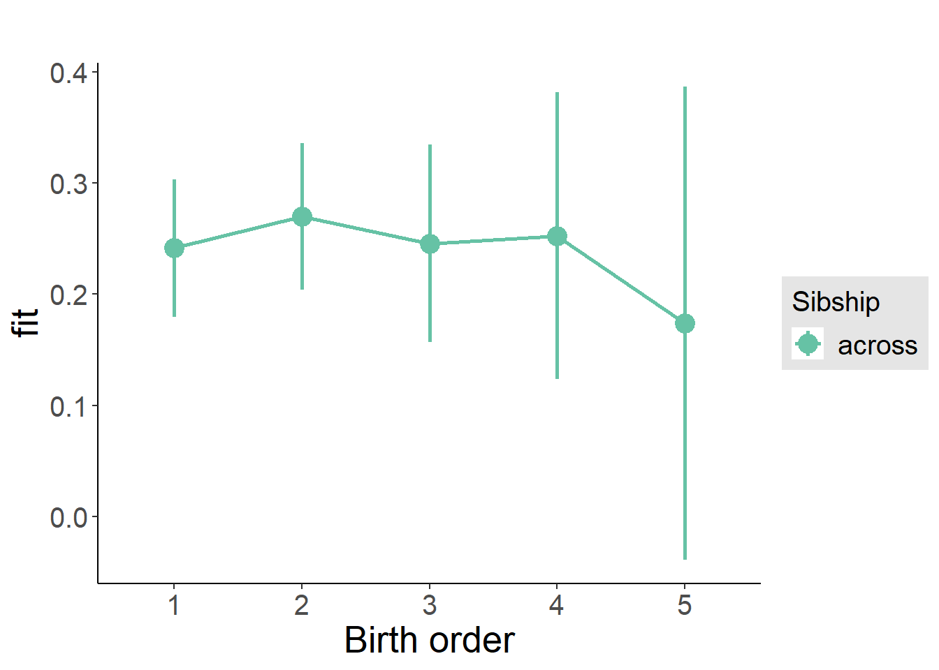
Add Interaction
Model Summary
m4_interaction = update(m3_birthorder_nonlinear, formula = . ~ . - birth_order_nonlinear - sibling_count + count_birth_order)
tidy(m4_interaction, conf.int = T, conf.level = 0.995)| effect | group | term | estimate | std.error | statistic | df | p.value | conf.low | conf.high |
|---|---|---|---|---|---|---|---|---|---|
| fixed | NA | (Intercept) | -3.208 | 0.2202 | -14.57 | 6716 | 2.403e-47 | -3.826 | -2.59 |
| fixed | NA | poly(age, 3, raw = TRUE)1 | 0.5573 | 0.04586 | 12.15 | 6638 | 1.29e-33 | 0.4285 | 0.686 |
| fixed | NA | poly(age, 3, raw = TRUE)2 | -0.02785 | 0.002964 | -9.396 | 6657 | 7.606e-21 | -0.03617 | -0.01953 |
| fixed | NA | poly(age, 3, raw = TRUE)3 | 0.0004442 | 0.00005942 | 7.475 | 6690 | 8.673e-14 | 0.0002774 | 0.000611 |
| fixed | NA | male | -0.176 | 0.02182 | -8.069 | 7191 | 8.238e-16 | -0.2373 | -0.1148 |
| fixed | NA | count_birth_order2/2 | 0.05523 | 0.03473 | 1.59 | 6001 | 0.1118 | -0.04225 | 0.1527 |
| fixed | NA | count_birth_order1/3 | 0.03204 | 0.04035 | 0.794 | 7484 | 0.4272 | -0.08124 | 0.1453 |
| fixed | NA | count_birth_order2/3 | 0.0281 | 0.03877 | 0.7248 | 7495 | 0.4686 | -0.08074 | 0.1369 |
| fixed | NA | count_birth_order3/3 | -0.0193 | 0.04248 | -0.4543 | 7509 | 0.6496 | -0.1386 | 0.09995 |
| fixed | NA | count_birth_order1/4 | -0.07964 | 0.06391 | -1.246 | 7422 | 0.2128 | -0.259 | 0.09976 |
| fixed | NA | count_birth_order2/4 | -0.06614 | 0.05597 | -1.182 | 7495 | 0.2374 | -0.2232 | 0.09097 |
| fixed | NA | count_birth_order3/4 | -0.009582 | 0.05339 | -0.1795 | 7492 | 0.8576 | -0.1594 | 0.1403 |
| fixed | NA | count_birth_order4/4 | -0.007008 | 0.05282 | -0.1327 | 7509 | 0.8945 | -0.1553 | 0.1413 |
| fixed | NA | count_birth_order1/5 | -0.07898 | 0.1118 | -0.7063 | 6753 | 0.48 | -0.3929 | 0.2349 |
| fixed | NA | count_birth_order2/5 | -0.06533 | 0.09944 | -0.657 | 7025 | 0.5112 | -0.3445 | 0.2138 |
| fixed | NA | count_birth_order3/5 | -0.07808 | 0.08398 | -0.9297 | 7301 | 0.3525 | -0.3138 | 0.1577 |
| fixed | NA | count_birth_order4/5 | -0.1593 | 0.06933 | -2.298 | 7497 | 0.0216 | -0.3539 | 0.0353 |
| fixed | NA | count_birth_order5/5 | -0.191 | 0.06718 | -2.843 | 7509 | 0.004485 | -0.3796 | -0.002399 |
| ran_pars | mother_pidlink | sd__(Intercept) | 0.4732 | NA | NA | NA | NA | NA | NA |
| ran_pars | Residual | sd__Observation | 0.8425 | NA | NA | NA | NA | NA | NA |
Coefficient Plot
plot_birthorder(m4_interaction)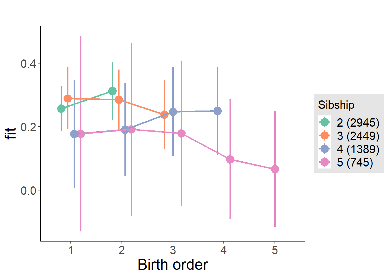
Model Comparison
###### Model 1 - Model 2
anova(m1_covariates_only, m2_birthorder_linear, m3_birthorder_nonlinear, m4_interaction)
## refitting model(s) with ML (instead of REML)| Df | AIC | BIC | logLik | deviance | Chisq | Chi Df | Pr(>Chisq) |
|---|---|---|---|---|---|---|---|
| 10 | 20687 | 20756 | -10333 | 20667 | NA | NA | NA |
| 11 | 20689 | 20765 | -10333 | 20667 | 0.000003839 | 1 | 0.9984 |
| 14 | 20692 | 20789 | -10332 | 20664 | 2.596 | 3 | 0.4581 |
| 20 | 20699 | 20837 | -10329 | 20659 | 5.37 | 6 | 0.4972 |
Maternal pregnancy order
outcome_preg_m1 <- update(m2_birthorder_linear, data = birthorder %>%
mutate(sibling_count = sibling_count_uterus_preg_factor,
birth_order_nonlinear = birthorder_uterus_preg_factor,
birth_order = birthorder_uterus_preg,
count_birth_order = count_birthorder_uterus_preg
) %>%
filter(sibling_count != "1"))
compare_models_markdown(outcome_preg_m1)Basic Model
Model Summary
m1_covariates_only <- update(m2_birthorder_linear, formula = . ~ . - birth_order)
tidy(m1_covariates_only, conf.int = T, conf.level = 0.995)| effect | group | term | estimate | std.error | statistic | df | p.value | conf.low | conf.high |
|---|---|---|---|---|---|---|---|---|---|
| fixed | NA | (Intercept) | -3.174 | 0.2233 | -14.21 | 6328 | 3.799e-45 | -3.801 | -2.547 |
| fixed | NA | poly(age, 3, raw = TRUE)1 | 0.5569 | 0.04701 | 11.85 | 6323 | 4.888e-32 | 0.425 | 0.6889 |
| fixed | NA | poly(age, 3, raw = TRUE)2 | -0.02805 | 0.00305 | -9.198 | 6361 | 4.867e-20 | -0.03662 | -0.01949 |
| fixed | NA | poly(age, 3, raw = TRUE)3 | 0.0004512 | 0.00006132 | 7.357 | 6392 | 2.11e-13 | 0.000279 | 0.0006233 |
| fixed | NA | male | -0.1854 | 0.02234 | -8.298 | 6863 | 1.263e-16 | -0.2481 | -0.1227 |
| fixed | NA | sibling_count3 | 0.02048 | 0.02977 | 0.6879 | 4765 | 0.4915 | -0.06308 | 0.104 |
| fixed | NA | sibling_count4 | -0.04367 | 0.03496 | -1.249 | 4248 | 0.2116 | -0.1418 | 0.05445 |
| fixed | NA | sibling_count5 | -0.05311 | 0.04092 | -1.298 | 3862 | 0.1944 | -0.168 | 0.06175 |
| ran_pars | mother_pidlink | sd__(Intercept) | 0.4666 | NA | NA | NA | NA | NA | NA |
| ran_pars | Residual | sd__Observation | 0.8447 | NA | NA | NA | NA | NA | NA |
Coefficient Plot
plot(allEffects(m1_covariates_only, confidence.level = 0.995))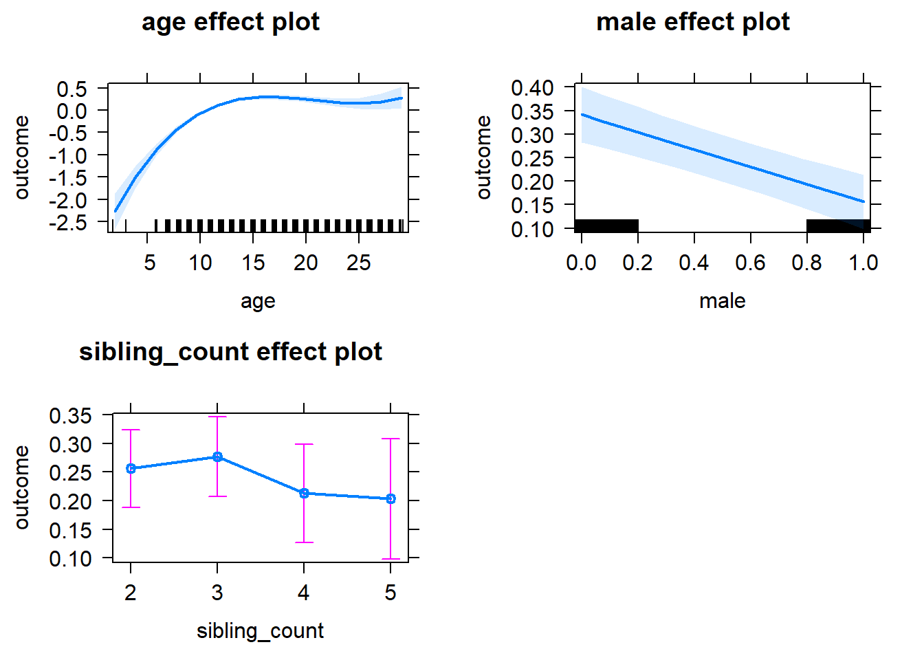
Add Birth Order Linear
Model Summary
tidy(m2_birthorder_linear, conf.int = T, conf.level = 0.995)| effect | group | term | estimate | std.error | statistic | df | p.value | conf.low | conf.high |
|---|---|---|---|---|---|---|---|---|---|
| fixed | NA | (Intercept) | -3.166 | 0.2263 | -13.99 | 6434 | 7.553e-44 | -3.801 | -2.531 |
| fixed | NA | birth_order | -0.002726 | 0.01298 | -0.21 | 6980 | 0.8337 | -0.03916 | 0.03371 |
| fixed | NA | poly(age, 3, raw = TRUE)1 | 0.5564 | 0.0471 | 11.81 | 6337 | 7.184e-32 | 0.4242 | 0.6886 |
| fixed | NA | poly(age, 3, raw = TRUE)2 | -0.02803 | 0.003052 | -9.183 | 6359 | 5.577e-20 | -0.0366 | -0.01946 |
| fixed | NA | poly(age, 3, raw = TRUE)3 | 0.0004508 | 0.00006135 | 7.348 | 6388 | 2.255e-13 | 0.0002786 | 0.000623 |
| fixed | NA | male | -0.1853 | 0.02234 | -8.294 | 6863 | 1.305e-16 | -0.248 | -0.1226 |
| fixed | NA | sibling_count3 | 0.02215 | 0.03081 | 0.7188 | 4873 | 0.4723 | -0.06435 | 0.1086 |
| fixed | NA | sibling_count4 | -0.03989 | 0.03931 | -1.015 | 4649 | 0.3102 | -0.1502 | 0.07044 |
| fixed | NA | sibling_count5 | -0.04716 | 0.04976 | -0.9478 | 4639 | 0.3433 | -0.1868 | 0.09251 |
| ran_pars | mother_pidlink | sd__(Intercept) | 0.4665 | NA | NA | NA | NA | NA | NA |
| ran_pars | Residual | sd__Observation | 0.8448 | NA | NA | NA | NA | NA | NA |
Coefficient Plot
plot_birthorder2(m2_birthorder_linear, separate = FALSE)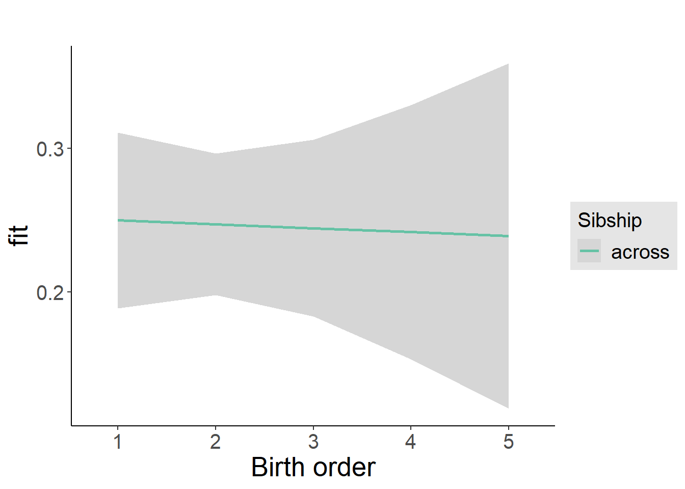
Add Birth Order Factor
Model Summary
m3_birthorder_nonlinear = update(m1_covariates_only, formula = . ~ . + birth_order_nonlinear)
tidy(m3_birthorder_nonlinear, conf.int = T, conf.level = 0.995)| effect | group | term | estimate | std.error | statistic | df | p.value | conf.low | conf.high |
|---|---|---|---|---|---|---|---|---|---|
| fixed | NA | (Intercept) | -3.179 | 0.2249 | -14.13 | 6401 | 1.1e-44 | -3.811 | -2.548 |
| fixed | NA | poly(age, 3, raw = TRUE)1 | 0.5565 | 0.04711 | 11.81 | 6337 | 7.175e-32 | 0.4243 | 0.6887 |
| fixed | NA | poly(age, 3, raw = TRUE)2 | -0.028 | 0.003053 | -9.171 | 6358 | 6.204e-20 | -0.03657 | -0.01943 |
| fixed | NA | poly(age, 3, raw = TRUE)3 | 0.0004496 | 0.00006136 | 7.328 | 6387 | 2.625e-13 | 0.0002774 | 0.0006219 |
| fixed | NA | male | -0.1858 | 0.02234 | -8.319 | 6860 | 1.065e-16 | -0.2486 | -0.1231 |
| fixed | NA | sibling_count3 | 0.01029 | 0.03157 | 0.3258 | 5132 | 0.7446 | -0.07834 | 0.09891 |
| fixed | NA | sibling_count4 | -0.04726 | 0.04033 | -1.172 | 4865 | 0.2412 | -0.1605 | 0.06593 |
| fixed | NA | sibling_count5 | -0.02709 | 0.05114 | -0.5298 | 4745 | 0.5963 | -0.1706 | 0.1164 |
| fixed | NA | birth_order_nonlinear2 | 0.01691 | 0.02603 | 0.6497 | 5343 | 0.5159 | -0.05616 | 0.08998 |
| fixed | NA | birth_order_nonlinear3 | 0.03612 | 0.03547 | 1.018 | 6257 | 0.3085 | -0.06344 | 0.1357 |
| fixed | NA | birth_order_nonlinear4 | -0.01534 | 0.04913 | -0.3123 | 6586 | 0.7549 | -0.1532 | 0.1226 |
| fixed | NA | birth_order_nonlinear5 | -0.0896 | 0.07324 | -1.223 | 6585 | 0.2213 | -0.2952 | 0.116 |
| ran_pars | mother_pidlink | sd__(Intercept) | 0.4669 | NA | NA | NA | NA | NA | NA |
| ran_pars | Residual | sd__Observation | 0.8446 | NA | NA | NA | NA | NA | NA |
Coefficient Plot
plot_birthorder(m3_birthorder_nonlinear, separate = FALSE)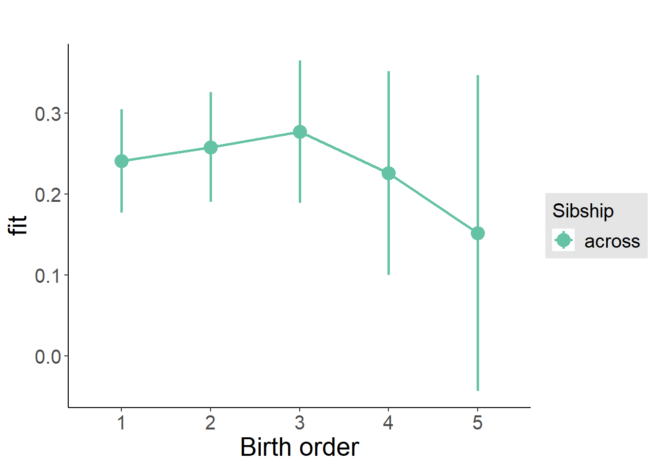
Add Interaction
Model Summary
m4_interaction = update(m3_birthorder_nonlinear, formula = . ~ . - birth_order_nonlinear - sibling_count + count_birth_order)
tidy(m4_interaction, conf.int = T, conf.level = 0.995)| effect | group | term | estimate | std.error | statistic | df | p.value | conf.low | conf.high |
|---|---|---|---|---|---|---|---|---|---|
| fixed | NA | (Intercept) | -3.183 | 0.2258 | -14.1 | 6412 | 1.851e-44 | -3.817 | -2.549 |
| fixed | NA | poly(age, 3, raw = TRUE)1 | 0.5551 | 0.04717 | 11.77 | 6344 | 1.226e-31 | 0.4227 | 0.6875 |
| fixed | NA | poly(age, 3, raw = TRUE)2 | -0.0279 | 0.003057 | -9.127 | 6359 | 9.329e-20 | -0.03648 | -0.01932 |
| fixed | NA | poly(age, 3, raw = TRUE)3 | 0.0004476 | 0.00006144 | 7.285 | 6385 | 3.595e-13 | 0.0002752 | 0.0006201 |
| fixed | NA | male | -0.1857 | 0.02234 | -8.313 | 6852 | 1.114e-16 | -0.2485 | -0.123 |
| fixed | NA | count_birth_order2/2 | 0.04363 | 0.03794 | 1.15 | 5669 | 0.2502 | -0.06287 | 0.1501 |
| fixed | NA | count_birth_order1/3 | 0.05878 | 0.04169 | 1.41 | 7136 | 0.1586 | -0.05824 | 0.1758 |
| fixed | NA | count_birth_order2/3 | 0.03572 | 0.04074 | 0.8769 | 7145 | 0.3806 | -0.07863 | 0.1501 |
| fixed | NA | count_birth_order3/3 | 0.009043 | 0.04469 | 0.2023 | 7152 | 0.8397 | -0.1164 | 0.1345 |
| fixed | NA | count_birth_order1/4 | -0.1252 | 0.06235 | -2.008 | 7101 | 0.04471 | -0.3002 | 0.04984 |
| fixed | NA | count_birth_order2/4 | -0.05209 | 0.0559 | -0.932 | 7130 | 0.3514 | -0.209 | 0.1048 |
| fixed | NA | count_birth_order3/4 | 0.04482 | 0.05346 | 0.8385 | 7135 | 0.4018 | -0.1052 | 0.1949 |
| fixed | NA | count_birth_order4/4 | -0.01274 | 0.05398 | -0.2361 | 7152 | 0.8134 | -0.1643 | 0.1388 |
| fixed | NA | count_birth_order1/5 | 0.04844 | 0.09105 | 0.532 | 6757 | 0.5947 | -0.2071 | 0.304 |
| fixed | NA | count_birth_order2/5 | -0.02286 | 0.08131 | -0.2812 | 6938 | 0.7786 | -0.2511 | 0.2054 |
| fixed | NA | count_birth_order3/5 | 0.07511 | 0.0729 | 1.03 | 7024 | 0.3029 | -0.1295 | 0.2797 |
| fixed | NA | count_birth_order4/5 | -0.09412 | 0.06707 | -1.403 | 7088 | 0.1605 | -0.2824 | 0.09414 |
| fixed | NA | count_birth_order5/5 | -0.1082 | 0.06446 | -1.678 | 7144 | 0.09332 | -0.2891 | 0.07275 |
| ran_pars | mother_pidlink | sd__(Intercept) | 0.4662 | NA | NA | NA | NA | NA | NA |
| ran_pars | Residual | sd__Observation | 0.8446 | NA | NA | NA | NA | NA | NA |
Coefficient Plot
plot_birthorder(m4_interaction)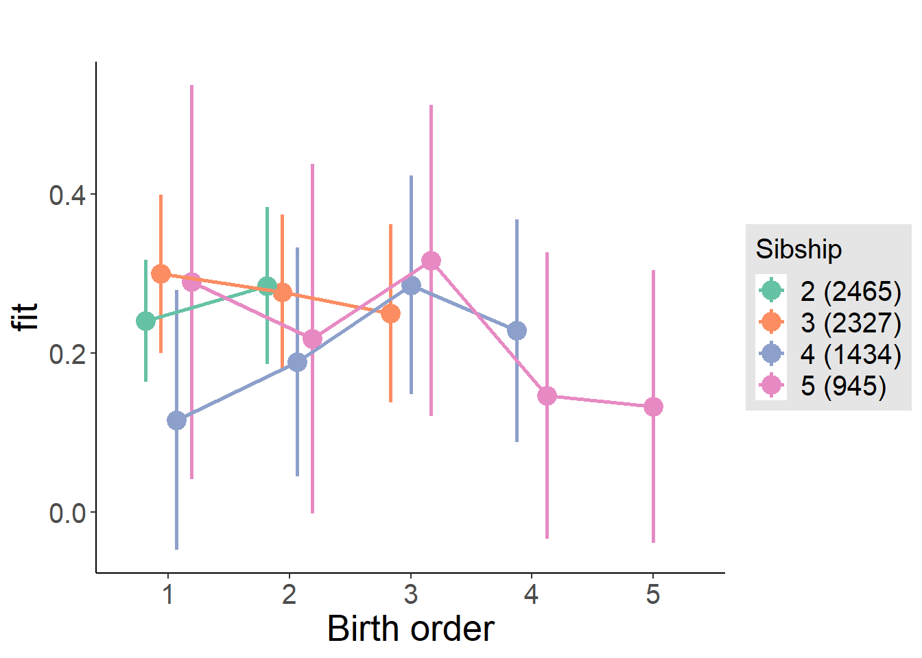
Model Comparison
###### Model 1 - Model 2
anova(m1_covariates_only, m2_birthorder_linear, m3_birthorder_nonlinear, m4_interaction)## refitting model(s) with ML (instead of REML)| Df | AIC | BIC | logLik | deviance | Chisq | Chi Df | Pr(>Chisq) |
|---|---|---|---|---|---|---|---|
| 10 | 19703 | 19772 | -9842 | 19683 | NA | NA | NA |
| 11 | 19705 | 19781 | -9842 | 19683 | 0.04432 | 1 | 0.8333 |
| 14 | 19707 | 19804 | -9840 | 19679 | 3.843 | 3 | 0.2789 |
| 20 | 19708 | 19846 | -9834 | 19668 | 10.89 | 6 | 0.09197 |
Parental full sibling order
outcome_parental_m1 <- update(m2_birthorder_linear, data = birthorder %>%
mutate(sibling_count = sibling_count_genes_factor,
birth_order_nonlinear = birthorder_genes_factor,
birth_order = birthorder_genes,
count_birth_order = count_birthorder_genes
) %>%
filter(sibling_count != "1"))
compare_models_markdown(outcome_parental_m1)Basic Model
Model Summary
m1_covariates_only <- update(m2_birthorder_linear, formula = . ~ . - birth_order)
tidy(m1_covariates_only, conf.int = T, conf.level = 0.995)| effect | group | term | estimate | std.error | statistic | df | p.value | conf.low | conf.high |
|---|---|---|---|---|---|---|---|---|---|
| fixed | NA | (Intercept) | -3.122 | 0.2188 | -14.27 | 6490 | 1.692e-45 | -3.736 | -2.508 |
| fixed | NA | poly(age, 3, raw = TRUE)1 | 0.5431 | 0.04589 | 11.84 | 6500 | 5.471e-32 | 0.4143 | 0.6719 |
| fixed | NA | poly(age, 3, raw = TRUE)2 | -0.02684 | 0.002966 | -9.049 | 6550 | 1.878e-19 | -0.03517 | -0.01851 |
| fixed | NA | poly(age, 3, raw = TRUE)3 | 0.0004225 | 0.00005944 | 7.107 | 6595 | 1.308e-12 | 0.0002556 | 0.0005893 |
| fixed | NA | male | -0.1756 | 0.02193 | -8.008 | 7062 | 1.353e-15 | -0.2371 | -0.114 |
| fixed | NA | sibling_count3 | -0.01287 | 0.02857 | -0.4505 | 4708 | 0.6523 | -0.09307 | 0.06733 |
| fixed | NA | sibling_count4 | -0.05807 | 0.03526 | -1.647 | 4028 | 0.09969 | -0.1571 | 0.04092 |
| fixed | NA | sibling_count5 | -0.1585 | 0.04656 | -3.404 | 3607 | 0.0006713 | -0.2892 | -0.0278 |
| ran_pars | mother_pidlink | sd__(Intercept) | 0.4762 | NA | NA | NA | NA | NA | NA |
| ran_pars | Residual | sd__Observation | 0.8379 | NA | NA | NA | NA | NA | NA |
Coefficient Plot
plot(allEffects(m1_covariates_only, confidence.level = 0.995))
Add Birth Order Linear
Model Summary
tidy(m2_birthorder_linear, conf.int = T, conf.level = 0.995)| effect | group | term | estimate | std.error | statistic | df | p.value | conf.low | conf.high |
|---|---|---|---|---|---|---|---|---|---|
| fixed | NA | (Intercept) | -3.133 | 0.2221 | -14.11 | 6618 | 1.495e-44 | -3.757 | -2.51 |
| fixed | NA | birth_order | 0.004036 | 0.01354 | 0.2981 | 7086 | 0.7656 | -0.03397 | 0.04204 |
| fixed | NA | poly(age, 3, raw = TRUE)1 | 0.5439 | 0.04597 | 11.83 | 6518 | 5.738e-32 | 0.4149 | 0.673 |
| fixed | NA | poly(age, 3, raw = TRUE)2 | -0.02687 | 0.002968 | -9.053 | 6548 | 1.805e-19 | -0.03521 | -0.01854 |
| fixed | NA | poly(age, 3, raw = TRUE)3 | 0.0004229 | 0.00005946 | 7.112 | 6591 | 1.264e-12 | 0.000256 | 0.0005898 |
| fixed | NA | male | -0.1757 | 0.02193 | -8.01 | 7061 | 1.333e-15 | -0.2372 | -0.1141 |
| fixed | NA | sibling_count3 | -0.01549 | 0.02989 | -0.5181 | 4823 | 0.6044 | -0.09938 | 0.06841 |
| fixed | NA | sibling_count4 | -0.0639 | 0.04033 | -1.584 | 4491 | 0.1132 | -0.1771 | 0.0493 |
| fixed | NA | sibling_count5 | -0.1681 | 0.05657 | -2.971 | 4429 | 0.002986 | -0.3269 | -0.009269 |
| ran_pars | mother_pidlink | sd__(Intercept) | 0.4763 | NA | NA | NA | NA | NA | NA |
| ran_pars | Residual | sd__Observation | 0.8379 | NA | NA | NA | NA | NA | NA |
Coefficient Plot
plot_birthorder2(m2_birthorder_linear, separate = FALSE)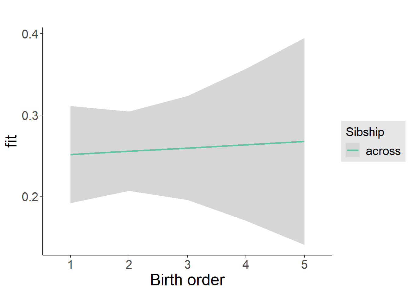
Add Birth Order Factor
Model Summary
m3_birthorder_nonlinear = update(m1_covariates_only, formula = . ~ . + birth_order_nonlinear)
tidy(m3_birthorder_nonlinear, conf.int = T, conf.level = 0.995)| effect | group | term | estimate | std.error | statistic | df | p.value | conf.low | conf.high |
|---|---|---|---|---|---|---|---|---|---|
| fixed | NA | (Intercept) | -3.139 | 0.2205 | -14.23 | 6583 | 2.613e-45 | -3.758 | -2.52 |
| fixed | NA | poly(age, 3, raw = TRUE)1 | 0.5441 | 0.04599 | 11.83 | 6522 | 5.62e-32 | 0.415 | 0.6732 |
| fixed | NA | poly(age, 3, raw = TRUE)2 | -0.02686 | 0.002969 | -9.048 | 6551 | 1.893e-19 | -0.0352 | -0.01853 |
| fixed | NA | poly(age, 3, raw = TRUE)3 | 0.0004223 | 0.00005947 | 7.1 | 6593 | 1.375e-12 | 0.0002553 | 0.0005892 |
| fixed | NA | male | -0.1761 | 0.02194 | -8.027 | 7061 | 1.159e-15 | -0.2377 | -0.1145 |
| fixed | NA | sibling_count3 | -0.01427 | 0.03064 | -0.4656 | 5112 | 0.6415 | -0.1003 | 0.07174 |
| fixed | NA | sibling_count4 | -0.07048 | 0.04136 | -1.704 | 4720 | 0.08845 | -0.1866 | 0.04562 |
| fixed | NA | sibling_count5 | -0.1424 | 0.05976 | -2.383 | 4601 | 0.01722 | -0.3101 | 0.02536 |
| fixed | NA | birth_order_nonlinear2 | 0.02454 | 0.025 | 0.9815 | 5482 | 0.3264 | -0.04564 | 0.09472 |
| fixed | NA | birth_order_nonlinear3 | 0.003256 | 0.03568 | 0.09124 | 6279 | 0.9273 | -0.09691 | 0.1034 |
| fixed | NA | birth_order_nonlinear4 | 0.04629 | 0.05139 | 0.9007 | 6619 | 0.3678 | -0.09796 | 0.1905 |
| fixed | NA | birth_order_nonlinear5 | -0.07451 | 0.08389 | -0.8881 | 6742 | 0.3745 | -0.31 | 0.161 |
| ran_pars | mother_pidlink | sd__(Intercept) | 0.4754 | NA | NA | NA | NA | NA | NA |
| ran_pars | Residual | sd__Observation | 0.8383 | NA | NA | NA | NA | NA | NA |
Coefficient Plot
plot_birthorder(m3_birthorder_nonlinear, separate = FALSE)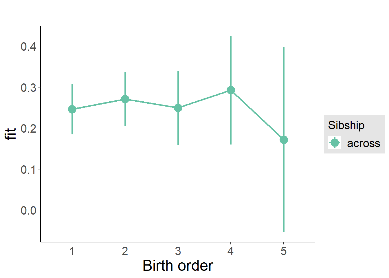
Add Interaction
Model Summary
m4_interaction = update(m3_birthorder_nonlinear, formula = . ~ . - birth_order_nonlinear - sibling_count + count_birth_order)
tidy(m4_interaction, conf.int = T, conf.level = 0.995)| effect | group | term | estimate | std.error | statistic | df | p.value | conf.low | conf.high |
|---|---|---|---|---|---|---|---|---|---|
| fixed | NA | (Intercept) | -3.156 | 0.2212 | -14.27 | 6599 | 1.694e-45 | -3.777 | -2.535 |
| fixed | NA | poly(age, 3, raw = TRUE)1 | 0.5455 | 0.04605 | 11.85 | 6529 | 4.744e-32 | 0.4163 | 0.6748 |
| fixed | NA | poly(age, 3, raw = TRUE)2 | -0.02696 | 0.002973 | -9.069 | 6553 | 1.558e-19 | -0.03531 | -0.01862 |
| fixed | NA | poly(age, 3, raw = TRUE)3 | 0.0004244 | 0.00005955 | 7.126 | 6592 | 1.143e-12 | 0.0002572 | 0.0005915 |
| fixed | NA | male | -0.1758 | 0.02194 | -8.01 | 7055 | 1.336e-15 | -0.2373 | -0.1142 |
| fixed | NA | count_birth_order2/2 | 0.05559 | 0.03435 | 1.619 | 5844 | 0.1056 | -0.04082 | 0.152 |
| fixed | NA | count_birth_order1/3 | 0.02666 | 0.0405 | 0.6583 | 7346 | 0.5104 | -0.08703 | 0.1404 |
| fixed | NA | count_birth_order2/3 | 0.01778 | 0.03886 | 0.4576 | 7355 | 0.6473 | -0.0913 | 0.1269 |
| fixed | NA | count_birth_order3/3 | -0.02945 | 0.04264 | -0.6907 | 7370 | 0.4898 | -0.1491 | 0.09023 |
| fixed | NA | count_birth_order1/4 | -0.09389 | 0.06423 | -1.462 | 7293 | 0.1438 | -0.2742 | 0.08641 |
| fixed | NA | count_birth_order2/4 | -0.08455 | 0.05666 | -1.492 | 7354 | 0.1357 | -0.2436 | 0.0745 |
| fixed | NA | count_birth_order3/4 | -0.01305 | 0.05374 | -0.2428 | 7355 | 0.8082 | -0.1639 | 0.1378 |
| fixed | NA | count_birth_order4/4 | 0.009224 | 0.05353 | 0.1723 | 7369 | 0.8632 | -0.141 | 0.1595 |
| fixed | NA | count_birth_order1/5 | -0.05048 | 0.1116 | -0.4524 | 6739 | 0.651 | -0.3637 | 0.2627 |
| fixed | NA | count_birth_order2/5 | -0.1133 | 0.1066 | -1.062 | 6816 | 0.2883 | -0.4126 | 0.1861 |
| fixed | NA | count_birth_order3/5 | -0.104 | 0.08614 | -1.207 | 7205 | 0.2274 | -0.3458 | 0.1378 |
| fixed | NA | count_birth_order4/5 | -0.1239 | 0.07287 | -1.701 | 7355 | 0.08904 | -0.3285 | 0.08062 |
| fixed | NA | count_birth_order5/5 | -0.2064 | 0.07115 | -2.901 | 7369 | 0.003727 | -0.4061 | -0.006708 |
| ran_pars | mother_pidlink | sd__(Intercept) | 0.4745 | NA | NA | NA | NA | NA | NA |
| ran_pars | Residual | sd__Observation | 0.8387 | NA | NA | NA | NA | NA | NA |
Coefficient Plot
plot_birthorder(m4_interaction)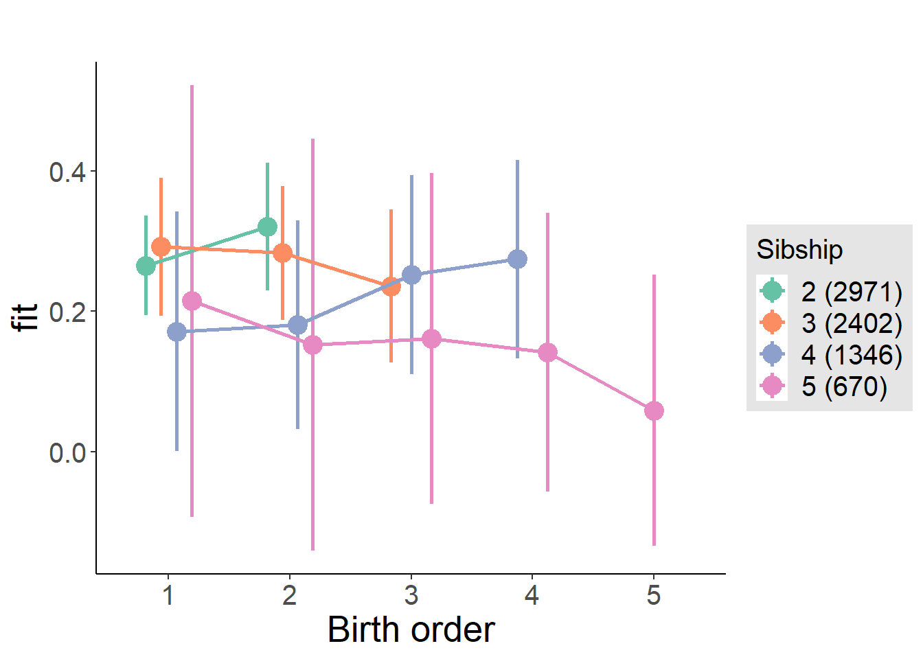
Model Comparison
###### Model 1 - Model 2
anova(m1_covariates_only, m2_birthorder_linear, m3_birthorder_nonlinear, m4_interaction)## refitting model(s) with ML (instead of REML)| Df | AIC | BIC | logLik | deviance | Chisq | Chi Df | Pr(>Chisq) |
|---|---|---|---|---|---|---|---|
| 10 | 20260 | 20329 | -10120 | 20240 | NA | NA | NA |
| 11 | 20262 | 20338 | -10120 | 20240 | 0.08875 | 1 | 0.7658 |
| 14 | 20265 | 20361 | -10118 | 20237 | 3.264 | 3 | 0.3527 |
| 20 | 20271 | 20409 | -10115 | 20231 | 5.983 | 6 | 0.4251 |
Compare birth order specifications
library(coefplot)
multiplot(outcome_naive_m1, outcome_preg_m1, outcome_uterus_m1, outcome_parental_m1, dodgeHeight = 0.6,
intercept = FALSE)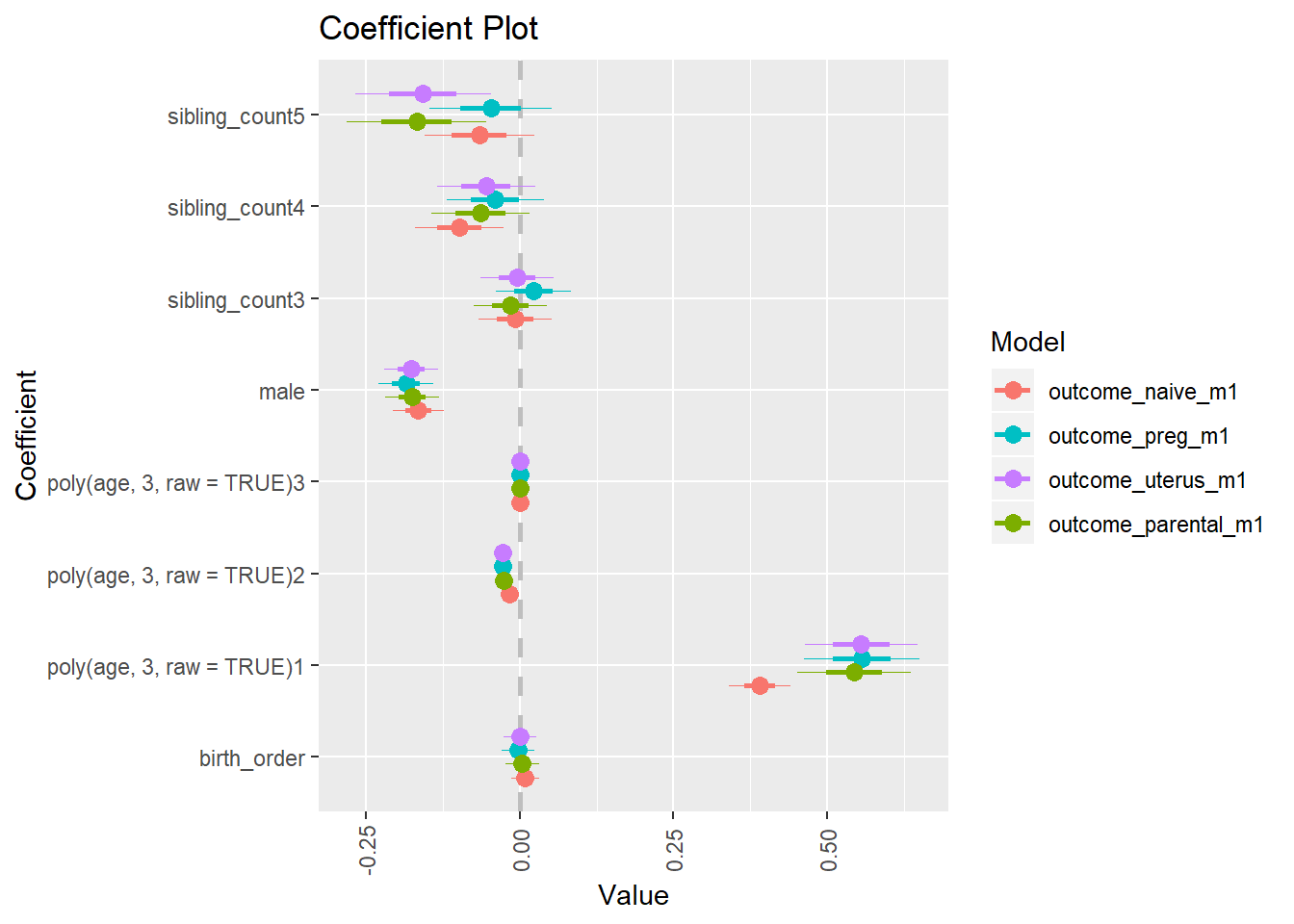
Raven 2007 old
birthorder <- birthorder %>% mutate(outcome = raven_2007_old)
model = lmer(outcome ~ birth_order + poly(age, 3, raw = TRUE) + male + sibling_count + (1 | mother_pidlink),
data = birthorder)
compare_birthorder_specs(model)Naive birth order
outcome_naive_m1 <- update(m2_birthorder_linear, data = birthorder %>%
mutate(sibling_count = sibling_count_naive_factor,
birth_order_nonlinear = birthorder_naive_factor,
birth_order = birthorder_naive,
count_birth_order = count_birthorder_naive) %>%
filter(sibling_count != "1"))
compare_models_markdown(outcome_naive_m1)Basic Model
Model Summary
m1_covariates_only <- update(m2_birthorder_linear, formula = . ~ . - birth_order)
tidy(m1_covariates_only, conf.int = T, conf.level = 0.995)| effect | group | term | estimate | std.error | statistic | df | p.value | conf.low | conf.high |
|---|---|---|---|---|---|---|---|---|---|
| fixed | NA | (Intercept) | -1.827 | 2.562 | -0.7131 | 3259 | 0.4759 | -9.017 | 5.364 |
| fixed | NA | poly(age, 3, raw = TRUE)1 | 0.234 | 0.2682 | 0.8728 | 3260 | 0.3828 | -0.5187 | 0.9868 |
| fixed | NA | poly(age, 3, raw = TRUE)2 | -0.008346 | 0.009243 | -0.903 | 3261 | 0.3666 | -0.03429 | 0.0176 |
| fixed | NA | poly(age, 3, raw = TRUE)3 | 0.00008858 | 0.0001049 | 0.8447 | 3262 | 0.3984 | -0.0002058 | 0.000383 |
| fixed | NA | male | 0.1557 | 0.03189 | 4.883 | 3085 | 0.000001098 | 0.0662 | 0.2452 |
| fixed | NA | sibling_count3 | -0.02541 | 0.0538 | -0.4724 | 2391 | 0.6367 | -0.1764 | 0.1256 |
| fixed | NA | sibling_count4 | -0.1124 | 0.05256 | -2.139 | 2281 | 0.03253 | -0.26 | 0.0351 |
| fixed | NA | sibling_count5 | -0.02315 | 0.05334 | -0.434 | 2116 | 0.6643 | -0.1729 | 0.1266 |
| ran_pars | mother_pidlink | sd__(Intercept) | 0.4768 | NA | NA | NA | NA | NA | NA |
| ran_pars | Residual | sd__Observation | 0.8043 | NA | NA | NA | NA | NA | NA |
Coefficient Plot
plot(allEffects(m1_covariates_only, confidence.level = 0.995))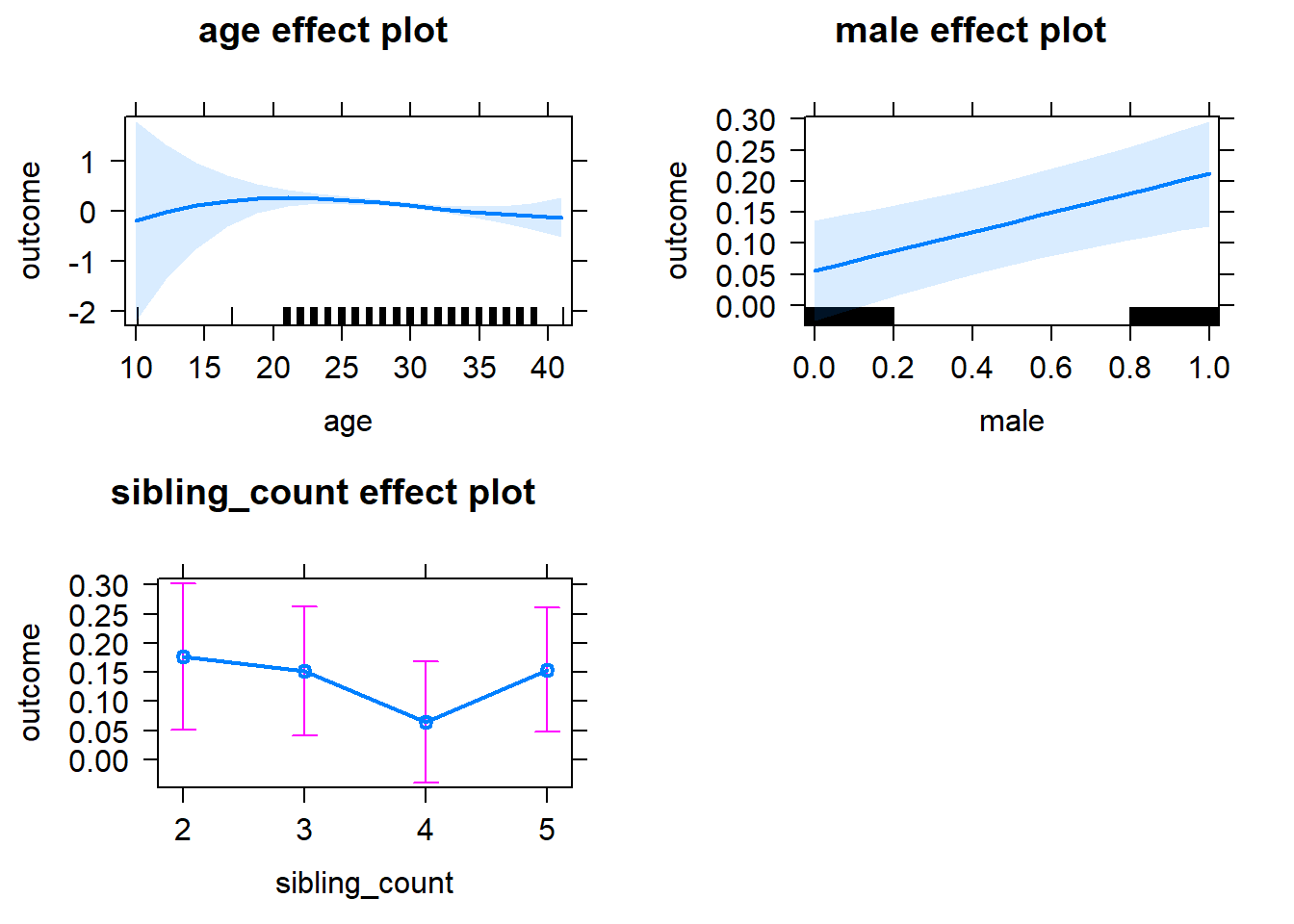
Add Birth Order Linear
Model Summary
tidy(m2_birthorder_linear, conf.int = T, conf.level = 0.995)| effect | group | term | estimate | std.error | statistic | df | p.value | conf.low | conf.high |
|---|---|---|---|---|---|---|---|---|---|
| fixed | NA | (Intercept) | -1.655 | 2.562 | -0.646 | 3259 | 0.5183 | -8.847 | 5.537 |
| fixed | NA | birth_order | -0.02899 | 0.01461 | -1.984 | 2924 | 0.04735 | -0.07001 | 0.01203 |
| fixed | NA | poly(age, 3, raw = TRUE)1 | 0.2209 | 0.2681 | 0.824 | 3259 | 0.41 | -0.5317 | 0.9736 |
| fixed | NA | poly(age, 3, raw = TRUE)2 | -0.007904 | 0.009242 | -0.8552 | 3260 | 0.3925 | -0.03385 | 0.01804 |
| fixed | NA | poly(age, 3, raw = TRUE)3 | 0.0000836 | 0.0001049 | 0.7973 | 3261 | 0.4253 | -0.0002107 | 0.0003779 |
| fixed | NA | male | 0.1559 | 0.03187 | 4.891 | 3082 | 0.000001052 | 0.06644 | 0.2454 |
| fixed | NA | sibling_count3 | -0.01234 | 0.05419 | -0.2277 | 2426 | 0.8199 | -0.1644 | 0.1398 |
| fixed | NA | sibling_count4 | -0.08595 | 0.05422 | -1.585 | 2424 | 0.113 | -0.2381 | 0.06624 |
| fixed | NA | sibling_count5 | 0.01907 | 0.05742 | 0.3322 | 2437 | 0.7398 | -0.1421 | 0.1803 |
| ran_pars | mother_pidlink | sd__(Intercept) | 0.4775 | NA | NA | NA | NA | NA | NA |
| ran_pars | Residual | sd__Observation | 0.8035 | NA | NA | NA | NA | NA | NA |
Coefficient Plot
plot_birthorder2(m2_birthorder_linear, separate = FALSE)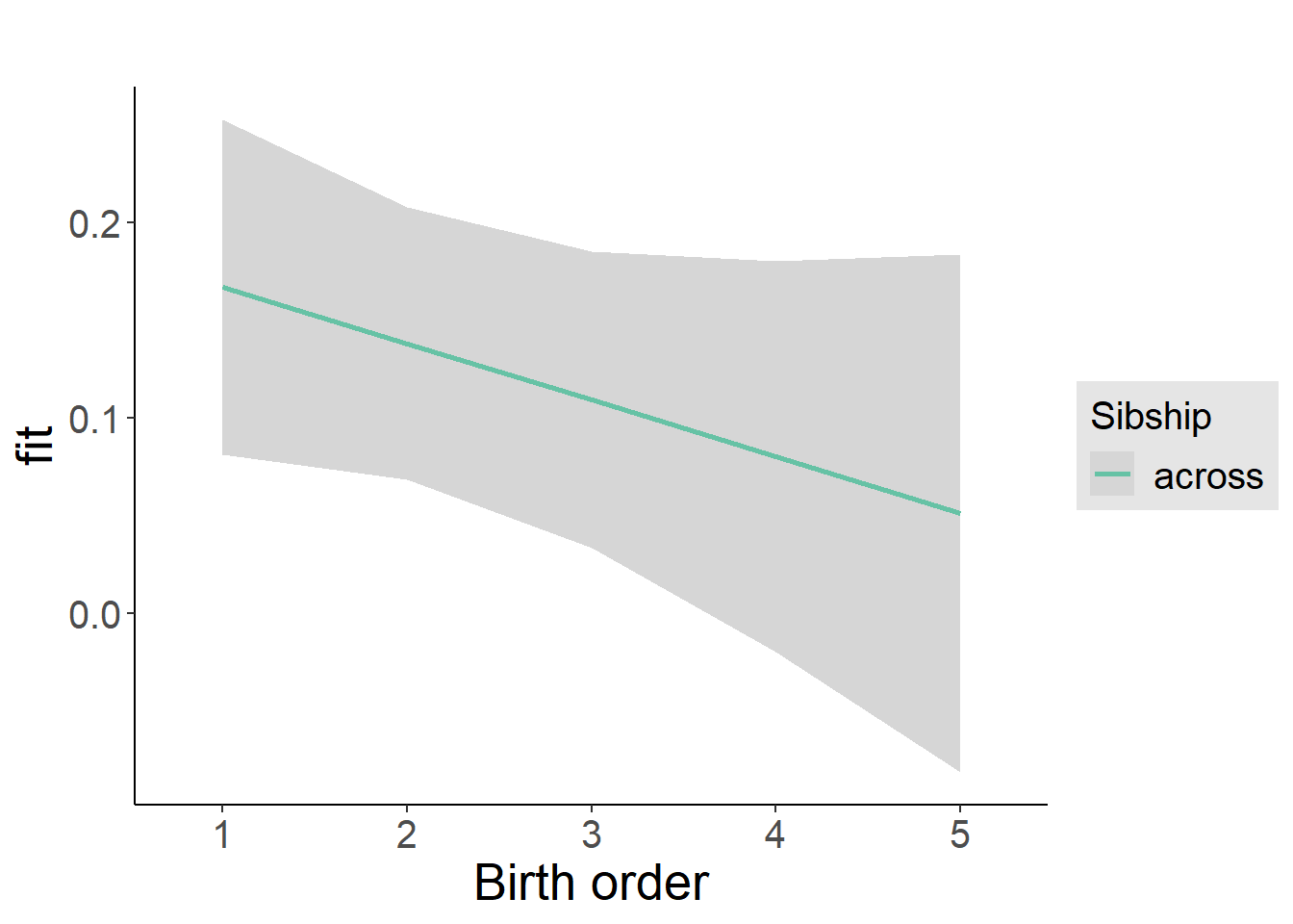
Add Birth Order Factor
Model Summary
m3_birthorder_nonlinear = update(m1_covariates_only, formula = . ~ . + birth_order_nonlinear)
tidy(m3_birthorder_nonlinear, conf.int = T, conf.level = 0.995)| effect | group | term | estimate | std.error | statistic | df | p.value | conf.low | conf.high |
|---|---|---|---|---|---|---|---|---|---|
| fixed | NA | (Intercept) | -1.464 | 2.563 | -0.5714 | 3256 | 0.5678 | -8.659 | 5.73 |
| fixed | NA | poly(age, 3, raw = TRUE)1 | 0.2027 | 0.2683 | 0.7557 | 3256 | 0.4499 | -0.5503 | 0.9558 |
| fixed | NA | poly(age, 3, raw = TRUE)2 | -0.007374 | 0.009247 | -0.7974 | 3257 | 0.4253 | -0.03333 | 0.01858 |
| fixed | NA | poly(age, 3, raw = TRUE)3 | 0.00007892 | 0.0001049 | 0.7522 | 3258 | 0.452 | -0.0002156 | 0.0003734 |
| fixed | NA | male | 0.1567 | 0.03186 | 4.918 | 3081 | 0.0000009198 | 0.06727 | 0.2462 |
| fixed | NA | sibling_count3 | -0.00198 | 0.05517 | -0.03589 | 2518 | 0.9714 | -0.1568 | 0.1529 |
| fixed | NA | sibling_count4 | -0.07838 | 0.05506 | -1.424 | 2517 | 0.1547 | -0.2329 | 0.07617 |
| fixed | NA | sibling_count5 | 0.004062 | 0.05791 | 0.07014 | 2482 | 0.9441 | -0.1585 | 0.1666 |
| fixed | NA | birth_order_nonlinear2 | -0.09006 | 0.03904 | -2.307 | 2552 | 0.02113 | -0.1996 | 0.01952 |
| fixed | NA | birth_order_nonlinear3 | -0.1224 | 0.04504 | -2.718 | 2536 | 0.006606 | -0.2489 | 0.003996 |
| fixed | NA | birth_order_nonlinear4 | -0.1101 | 0.05575 | -1.975 | 2700 | 0.04837 | -0.2666 | 0.04639 |
| fixed | NA | birth_order_nonlinear5 | -0.01848 | 0.0794 | -0.2328 | 2696 | 0.8159 | -0.2414 | 0.2044 |
| ran_pars | mother_pidlink | sd__(Intercept) | 0.4764 | NA | NA | NA | NA | NA | NA |
| ran_pars | Residual | sd__Observation | 0.8035 | NA | NA | NA | NA | NA | NA |
Coefficient Plot
plot_birthorder(m3_birthorder_nonlinear, separate = FALSE)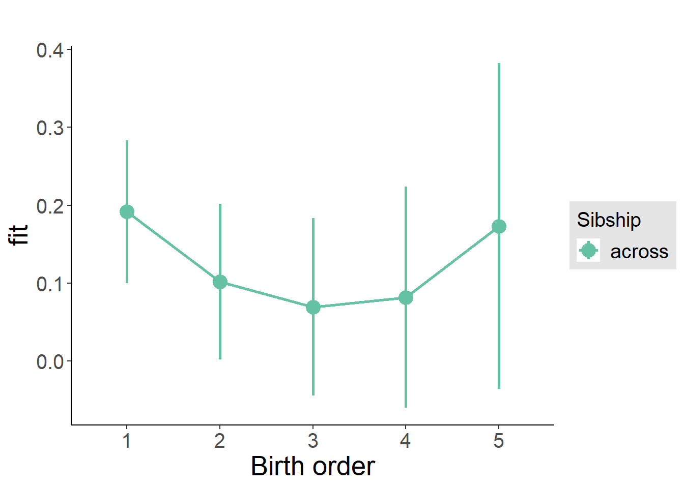
Add Interaction
Model Summary
m4_interaction = update(m3_birthorder_nonlinear, formula = . ~ . - birth_order_nonlinear - sibling_count + count_birth_order)
tidy(m4_interaction, conf.int = T, conf.level = 0.995)| effect | group | term | estimate | std.error | statistic | df | p.value | conf.low | conf.high |
|---|---|---|---|---|---|---|---|---|---|
| fixed | NA | (Intercept) | -1.778 | 2.564 | -0.6935 | 3250 | 0.4881 | -8.976 | 5.42 |
| fixed | NA | poly(age, 3, raw = TRUE)1 | 0.2353 | 0.2684 | 0.8766 | 3251 | 0.3808 | -0.5181 | 0.9887 |
| fixed | NA | poly(age, 3, raw = TRUE)2 | -0.008449 | 0.009251 | -0.9133 | 3251 | 0.3612 | -0.03442 | 0.01752 |
| fixed | NA | poly(age, 3, raw = TRUE)3 | 0.00009063 | 0.000105 | 0.8635 | 3252 | 0.3879 | -0.000204 | 0.0003852 |
| fixed | NA | male | 0.1548 | 0.03188 | 4.856 | 3078 | 0.000001258 | 0.06532 | 0.2443 |
| fixed | NA | count_birth_order2/2 | -0.1113 | 0.0741 | -1.502 | 2605 | 0.1333 | -0.3193 | 0.09671 |
| fixed | NA | count_birth_order1/3 | -0.02558 | 0.07353 | -0.348 | 3236 | 0.7279 | -0.232 | 0.1808 |
| fixed | NA | count_birth_order2/3 | -0.07059 | 0.0786 | -0.8981 | 3252 | 0.3692 | -0.2912 | 0.15 |
| fixed | NA | count_birth_order3/3 | -0.1446 | 0.07885 | -1.834 | 3252 | 0.06671 | -0.366 | 0.0767 |
| fixed | NA | count_birth_order1/4 | -0.04806 | 0.07578 | -0.6342 | 3249 | 0.526 | -0.2608 | 0.1646 |
| fixed | NA | count_birth_order2/4 | -0.1356 | 0.07907 | -1.715 | 3251 | 0.08638 | -0.3576 | 0.08632 |
| fixed | NA | count_birth_order3/4 | -0.311 | 0.0813 | -3.825 | 3242 | 0.0001331 | -0.5392 | -0.08278 |
| fixed | NA | count_birth_order4/4 | -0.2024 | 0.08206 | -2.467 | 3251 | 0.01369 | -0.4327 | 0.02794 |
| fixed | NA | count_birth_order1/5 | -0.05145 | 0.08312 | -0.619 | 3248 | 0.536 | -0.2848 | 0.1819 |
| fixed | NA | count_birth_order2/5 | -0.174 | 0.08473 | -2.054 | 3240 | 0.04009 | -0.4118 | 0.06384 |
| fixed | NA | count_birth_order3/5 | -0.004018 | 0.08368 | -0.04801 | 3232 | 0.9617 | -0.2389 | 0.2309 |
| fixed | NA | count_birth_order4/5 | -0.1149 | 0.08558 | -1.343 | 3218 | 0.1795 | -0.3552 | 0.1253 |
| fixed | NA | count_birth_order5/5 | -0.01877 | 0.08729 | -0.215 | 3237 | 0.8298 | -0.2638 | 0.2263 |
| ran_pars | mother_pidlink | sd__(Intercept) | 0.4728 | NA | NA | NA | NA | NA | NA |
| ran_pars | Residual | sd__Observation | 0.8045 | NA | NA | NA | NA | NA | NA |
Coefficient Plot
plot_birthorder(m4_interaction)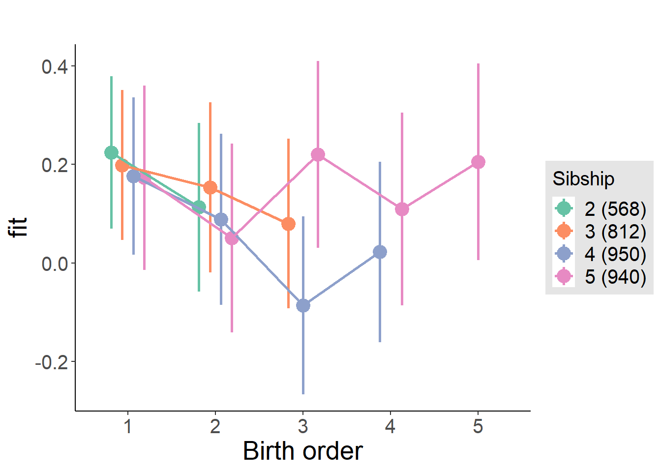
Model Comparison
###### Model 1 - Model 2
anova(m1_covariates_only, m2_birthorder_linear, m3_birthorder_nonlinear, m4_interaction)## refitting model(s) with ML (instead of REML)| Df | AIC | BIC | logLik | deviance | Chisq | Chi Df | Pr(>Chisq) |
|---|---|---|---|---|---|---|---|
| 10 | 8769 | 8830 | -4374 | 8749 | NA | NA | NA |
| 11 | 8767 | 8834 | -4372 | 8745 | 3.941 | 1 | 0.04712 |
| 14 | 8766 | 8851 | -4369 | 8738 | 6.58 | 3 | 0.08656 |
| 20 | 8768 | 8889 | -4364 | 8728 | 10.6 | 6 | 0.1017 |
Maternal birth order
outcome_uterus_m1 <- update(m2_birthorder_linear, data = birthorder %>%
mutate(sibling_count = sibling_count_uterus_alive_factor,
birth_order_nonlinear = birthorder_uterus_alive_factor,
birth_order = birthorder_uterus_alive,
count_birth_order = count_birthorder_uterus_alive) %>%
filter(sibling_count != "1"))
compare_models_markdown(outcome_uterus_m1)Basic Model
Model Summary
m1_covariates_only <- update(m2_birthorder_linear, formula = . ~ . - birth_order)
tidy(m1_covariates_only, conf.int = T, conf.level = 0.995)| effect | group | term | estimate | std.error | statistic | df | p.value | conf.low | conf.high |
|---|---|---|---|---|---|---|---|---|---|
| fixed | NA | (Intercept) | -2.945 | 4.169 | -0.7063 | 2326 | 0.4801 | -14.65 | 8.759 |
| fixed | NA | poly(age, 3, raw = TRUE)1 | 0.3379 | 0.436 | 0.775 | 2324 | 0.4384 | -0.8859 | 1.562 |
| fixed | NA | poly(age, 3, raw = TRUE)2 | -0.01145 | 0.01498 | -0.7649 | 2322 | 0.4444 | -0.05349 | 0.03058 |
| fixed | NA | poly(age, 3, raw = TRUE)3 | 0.000127 | 0.0001691 | 0.7509 | 2319 | 0.4528 | -0.0003476 | 0.0006016 |
| fixed | NA | male | 0.05754 | 0.03241 | 1.775 | 2434 | 0.07597 | -0.03344 | 0.1485 |
| fixed | NA | sibling_count3 | -0.003758 | 0.04882 | -0.07698 | 1772 | 0.9386 | -0.1408 | 0.1333 |
| fixed | NA | sibling_count4 | -0.1099 | 0.05052 | -2.176 | 1670 | 0.0297 | -0.2517 | 0.03189 |
| fixed | NA | sibling_count5 | -0.1784 | 0.05512 | -3.236 | 1590 | 0.001235 | -0.3331 | -0.02367 |
| ran_pars | mother_pidlink | sd__(Intercept) | 0.393 | NA | NA | NA | NA | NA | NA |
| ran_pars | Residual | sd__Observation | 0.735 | NA | NA | NA | NA | NA | NA |
Coefficient Plot
plot(allEffects(m1_covariates_only, confidence.level = 0.995))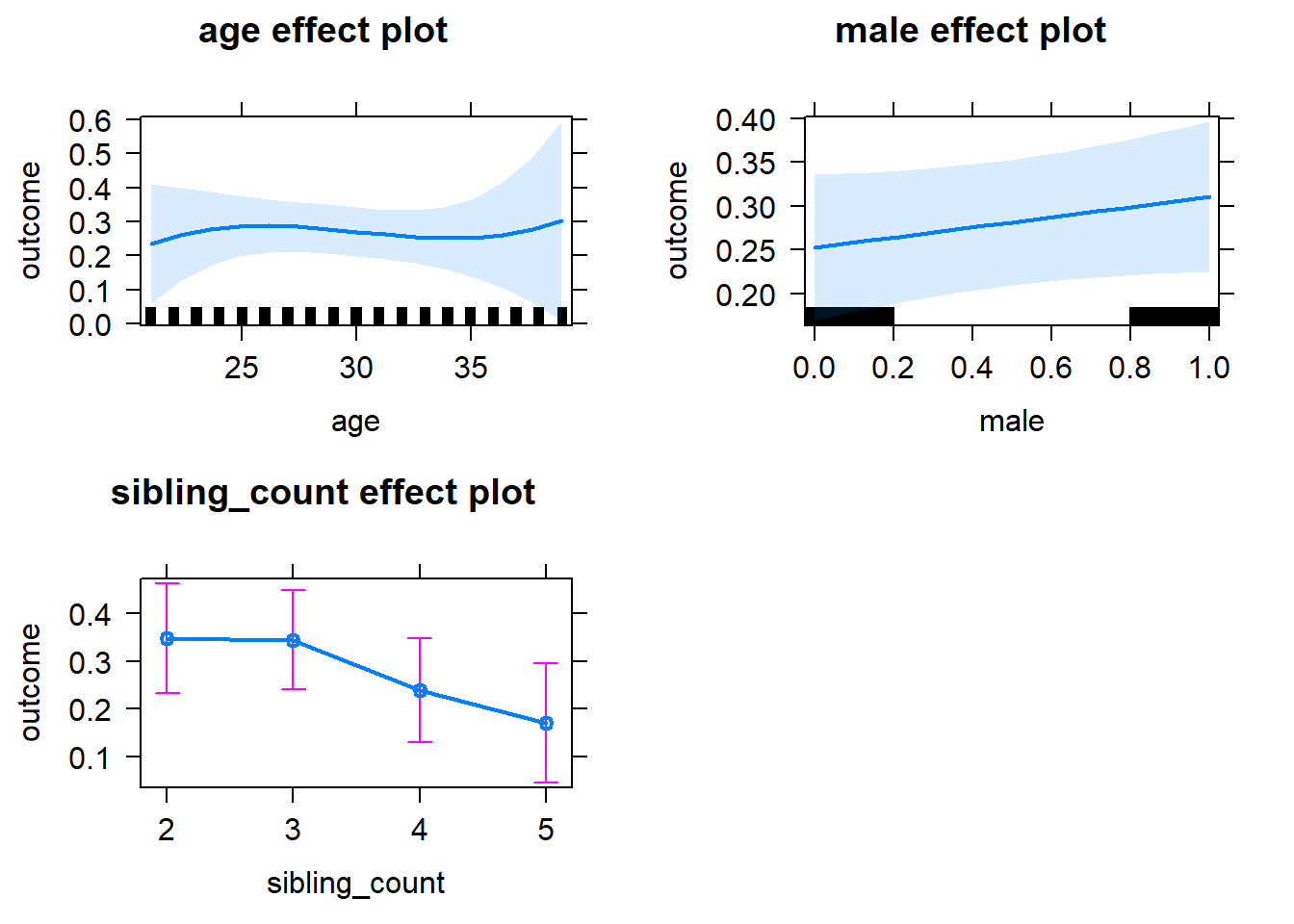
Add Birth Order Linear
Model Summary
tidy(m2_birthorder_linear, conf.int = T, conf.level = 0.995)| effect | group | term | estimate | std.error | statistic | df | p.value | conf.low | conf.high |
|---|---|---|---|---|---|---|---|---|---|
| fixed | NA | (Intercept) | -3.078 | 4.172 | -0.7378 | 2325 | 0.4607 | -14.79 | 8.632 |
| fixed | NA | birth_order | 0.01523 | 0.01653 | 0.9214 | 2463 | 0.3569 | -0.03117 | 0.06162 |
| fixed | NA | poly(age, 3, raw = TRUE)1 | 0.35 | 0.4361 | 0.8026 | 2322 | 0.4223 | -0.8742 | 1.574 |
| fixed | NA | poly(age, 3, raw = TRUE)2 | -0.0119 | 0.01498 | -0.7944 | 2320 | 0.4271 | -0.05396 | 0.03015 |
| fixed | NA | poly(age, 3, raw = TRUE)3 | 0.0001326 | 0.0001692 | 0.7835 | 2318 | 0.4334 | -0.0003423 | 0.0006074 |
| fixed | NA | male | 0.05732 | 0.03241 | 1.769 | 2432 | 0.0771 | -0.03366 | 0.1483 |
| fixed | NA | sibling_count3 | -0.01016 | 0.04932 | -0.206 | 1794 | 0.8368 | -0.1486 | 0.1283 |
| fixed | NA | sibling_count4 | -0.126 | 0.05348 | -2.357 | 1746 | 0.01855 | -0.2761 | 0.02409 |
| fixed | NA | sibling_count5 | -0.2053 | 0.06237 | -3.291 | 1823 | 0.001016 | -0.3803 | -0.03021 |
| ran_pars | mother_pidlink | sd__(Intercept) | 0.3942 | NA | NA | NA | NA | NA | NA |
| ran_pars | Residual | sd__Observation | 0.7345 | NA | NA | NA | NA | NA | NA |
Coefficient Plot
plot_birthorder2(m2_birthorder_linear, separate = FALSE)
Add Birth Order Factor
Model Summary
m3_birthorder_nonlinear = update(m1_covariates_only, formula = . ~ . + birth_order_nonlinear)
tidy(m3_birthorder_nonlinear, conf.int = T, conf.level = 0.995)| effect | group | term | estimate | std.error | statistic | df | p.value | conf.low | conf.high |
|---|---|---|---|---|---|---|---|---|---|
| fixed | NA | (Intercept) | -3.107 | 4.175 | -0.7441 | 2321 | 0.4569 | -14.83 | 8.614 |
| fixed | NA | poly(age, 3, raw = TRUE)1 | 0.3557 | 0.4366 | 0.8148 | 2318 | 0.4153 | -0.8698 | 1.581 |
| fixed | NA | poly(age, 3, raw = TRUE)2 | -0.01211 | 0.015 | -0.8072 | 2315 | 0.4196 | -0.05421 | 0.02999 |
| fixed | NA | poly(age, 3, raw = TRUE)3 | 0.0001349 | 0.0001694 | 0.7968 | 2313 | 0.4256 | -0.0003404 | 0.0006103 |
| fixed | NA | male | 0.05711 | 0.03243 | 1.761 | 2429 | 0.07836 | -0.03393 | 0.1482 |
| fixed | NA | sibling_count3 | -0.01447 | 0.04989 | -0.2901 | 1848 | 0.7718 | -0.1545 | 0.1256 |
| fixed | NA | sibling_count4 | -0.1275 | 0.05425 | -2.351 | 1802 | 0.01883 | -0.2798 | 0.02474 |
| fixed | NA | sibling_count5 | -0.2101 | 0.06315 | -3.328 | 1859 | 0.0008926 | -0.3874 | -0.03288 |
| fixed | NA | birth_order_nonlinear2 | -0.004541 | 0.0385 | -0.118 | 1917 | 0.9061 | -0.1126 | 0.1035 |
| fixed | NA | birth_order_nonlinear3 | 0.04573 | 0.04747 | 0.9633 | 2103 | 0.3355 | -0.08752 | 0.179 |
| fixed | NA | birth_order_nonlinear4 | 0.0251 | 0.06298 | 0.3986 | 2334 | 0.6902 | -0.1517 | 0.2019 |
| fixed | NA | birth_order_nonlinear5 | 0.07403 | 0.09469 | 0.7818 | 2261 | 0.4344 | -0.1918 | 0.3398 |
| ran_pars | mother_pidlink | sd__(Intercept) | 0.3942 | NA | NA | NA | NA | NA | NA |
| ran_pars | Residual | sd__Observation | 0.7349 | NA | NA | NA | NA | NA | NA |
Coefficient Plot
plot_birthorder(m3_birthorder_nonlinear, separate = FALSE)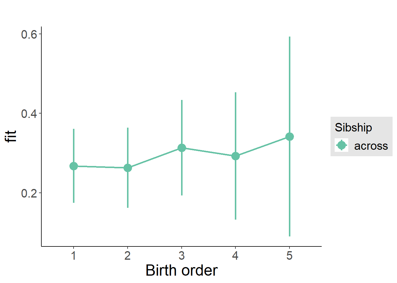
Add Interaction
Model Summary
m4_interaction = update(m3_birthorder_nonlinear, formula = . ~ . - birth_order_nonlinear - sibling_count + count_birth_order)
tidy(m4_interaction, conf.int = T, conf.level = 0.995)| effect | group | term | estimate | std.error | statistic | df | p.value | conf.low | conf.high |
|---|---|---|---|---|---|---|---|---|---|
| fixed | NA | (Intercept) | -3.288 | 4.175 | -0.7875 | 2313 | 0.4311 | -15.01 | 8.431 |
| fixed | NA | poly(age, 3, raw = TRUE)1 | 0.3785 | 0.4365 | 0.867 | 2311 | 0.386 | -0.8468 | 1.604 |
| fixed | NA | poly(age, 3, raw = TRUE)2 | -0.01294 | 0.015 | -0.8629 | 2308 | 0.3883 | -0.05504 | 0.02915 |
| fixed | NA | poly(age, 3, raw = TRUE)3 | 0.0001449 | 0.0001693 | 0.8559 | 2306 | 0.3921 | -0.0003304 | 0.0006202 |
| fixed | NA | male | 0.05816 | 0.03247 | 1.791 | 2425 | 0.07341 | -0.03299 | 0.1493 |
| fixed | NA | count_birth_order2/2 | -0.06829 | 0.06869 | -0.9942 | 1905 | 0.3203 | -0.2611 | 0.1245 |
| fixed | NA | count_birth_order1/3 | -0.05431 | 0.06277 | -0.8652 | 2510 | 0.387 | -0.2305 | 0.1219 |
| fixed | NA | count_birth_order2/3 | 0.01655 | 0.0688 | 0.2406 | 2531 | 0.8099 | -0.1766 | 0.2097 |
| fixed | NA | count_birth_order3/3 | -0.03883 | 0.07639 | -0.5083 | 2528 | 0.6113 | -0.2533 | 0.1756 |
| fixed | NA | count_birth_order1/4 | -0.1429 | 0.07346 | -1.945 | 2526 | 0.05193 | -0.3491 | 0.06335 |
| fixed | NA | count_birth_order2/4 | -0.1636 | 0.07503 | -2.181 | 2530 | 0.0293 | -0.3742 | 0.04699 |
| fixed | NA | count_birth_order3/4 | -0.1546 | 0.07604 | -2.034 | 2521 | 0.04209 | -0.3681 | 0.05881 |
| fixed | NA | count_birth_order4/4 | -0.06506 | 0.08254 | -0.7882 | 2525 | 0.4307 | -0.2968 | 0.1666 |
| fixed | NA | count_birth_order1/5 | -0.2747 | 0.09467 | -2.901 | 2529 | 0.003749 | -0.5404 | -0.008918 |
| fixed | NA | count_birth_order2/5 | -0.2925 | 0.09802 | -2.984 | 2507 | 0.002871 | -0.5677 | -0.01736 |
| fixed | NA | count_birth_order3/5 | -0.03308 | 0.08964 | -0.369 | 2502 | 0.7122 | -0.2847 | 0.2185 |
| fixed | NA | count_birth_order4/5 | -0.278 | 0.08875 | -3.133 | 2511 | 0.001751 | -0.5272 | -0.02892 |
| fixed | NA | count_birth_order5/5 | -0.1568 | 0.09316 | -1.683 | 2511 | 0.09251 | -0.4183 | 0.1047 |
| ran_pars | mother_pidlink | sd__(Intercept) | 0.3962 | NA | NA | NA | NA | NA | NA |
| ran_pars | Residual | sd__Observation | 0.7332 | NA | NA | NA | NA | NA | NA |
Coefficient Plot
plot_birthorder(m4_interaction)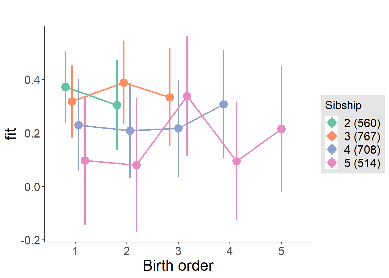
Model Comparison
###### Model 1 - Model 2
anova(m1_covariates_only, m2_birthorder_linear, m3_birthorder_nonlinear, m4_interaction)## refitting model(s) with ML (instead of REML)| Df | AIC | BIC | logLik | deviance | Chisq | Chi Df | Pr(>Chisq) |
|---|---|---|---|---|---|---|---|
| 10 | 6270 | 6328 | -3125 | 6250 | NA | NA | NA |
| 11 | 6271 | 6335 | -3125 | 6249 | 0.8474 | 1 | 0.3573 |
| 14 | 6276 | 6358 | -3124 | 6248 | 0.7468 | 3 | 0.8621 |
| 20 | 6278 | 6395 | -3119 | 6238 | 10.65 | 6 | 0.09966 |
Maternal pregnancy order
outcome_preg_m1 <- update(m2_birthorder_linear, data = birthorder %>%
mutate(sibling_count = sibling_count_uterus_preg_factor,
birth_order_nonlinear = birthorder_uterus_preg_factor,
birth_order = birthorder_uterus_preg,
count_birth_order = count_birthorder_uterus_preg
) %>%
filter(sibling_count != "1"))
compare_models_markdown(outcome_preg_m1)Basic Model
Model Summary
m1_covariates_only <- update(m2_birthorder_linear, formula = . ~ . - birth_order)
tidy(m1_covariates_only, conf.int = T, conf.level = 0.995)| effect | group | term | estimate | std.error | statistic | df | p.value | conf.low | conf.high |
|---|---|---|---|---|---|---|---|---|---|
| fixed | NA | (Intercept) | -1.121 | 4.391 | -0.2553 | 2134 | 0.7985 | -13.45 | 11.2 |
| fixed | NA | poly(age, 3, raw = TRUE)1 | 0.1369 | 0.4597 | 0.2979 | 2133 | 0.7658 | -1.153 | 1.427 |
| fixed | NA | poly(age, 3, raw = TRUE)2 | -0.004125 | 0.01581 | -0.261 | 2132 | 0.7941 | -0.0485 | 0.04025 |
| fixed | NA | poly(age, 3, raw = TRUE)3 | 0.00003911 | 0.0001787 | 0.2189 | 2130 | 0.8268 | -0.0004625 | 0.0005407 |
| fixed | NA | male | 0.06037 | 0.03382 | 1.785 | 2210 | 0.07441 | -0.03457 | 0.1553 |
| fixed | NA | sibling_count3 | -0.04486 | 0.0536 | -0.8369 | 1671 | 0.4028 | -0.1953 | 0.1056 |
| fixed | NA | sibling_count4 | -0.08056 | 0.0544 | -1.481 | 1594 | 0.1388 | -0.2333 | 0.07214 |
| fixed | NA | sibling_count5 | -0.1482 | 0.05662 | -2.617 | 1537 | 0.008945 | -0.3071 | 0.01073 |
| ran_pars | mother_pidlink | sd__(Intercept) | 0.3838 | NA | NA | NA | NA | NA | NA |
| ran_pars | Residual | sd__Observation | 0.7351 | NA | NA | NA | NA | NA | NA |
Coefficient Plot
plot(allEffects(m1_covariates_only, confidence.level = 0.995))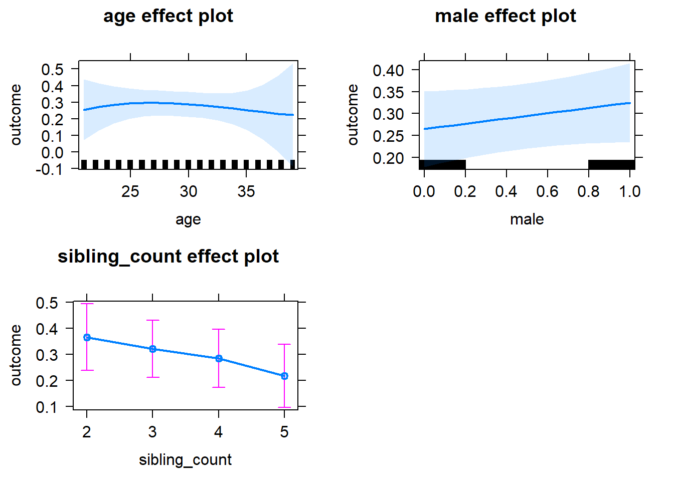
Add Birth Order Linear
Model Summary
tidy(m2_birthorder_linear, conf.int = T, conf.level = 0.995)| effect | group | term | estimate | std.error | statistic | df | p.value | conf.low | conf.high |
|---|---|---|---|---|---|---|---|---|---|
| fixed | NA | (Intercept) | -1.091 | 4.396 | -0.2481 | 2134 | 0.8041 | -13.43 | 11.25 |
| fixed | NA | birth_order | -0.002983 | 0.01665 | -0.1792 | 2260 | 0.8578 | -0.04971 | 0.04375 |
| fixed | NA | poly(age, 3, raw = TRUE)1 | 0.1341 | 0.46 | 0.2915 | 2133 | 0.7707 | -1.157 | 1.425 |
| fixed | NA | poly(age, 3, raw = TRUE)2 | -0.004023 | 0.01582 | -0.2543 | 2131 | 0.7993 | -0.04844 | 0.04039 |
| fixed | NA | poly(age, 3, raw = TRUE)3 | 0.00003786 | 0.0001789 | 0.2117 | 2129 | 0.8324 | -0.0004642 | 0.0005399 |
| fixed | NA | male | 0.06033 | 0.03383 | 1.783 | 2209 | 0.07469 | -0.03464 | 0.1553 |
| fixed | NA | sibling_count3 | -0.04355 | 0.05411 | -0.8049 | 1685 | 0.421 | -0.1954 | 0.1083 |
| fixed | NA | sibling_count4 | -0.07766 | 0.05677 | -1.368 | 1645 | 0.1715 | -0.237 | 0.0817 |
| fixed | NA | sibling_count5 | -0.1435 | 0.06243 | -2.298 | 1699 | 0.02167 | -0.3187 | 0.03177 |
| ran_pars | mother_pidlink | sd__(Intercept) | 0.3837 | NA | NA | NA | NA | NA | NA |
| ran_pars | Residual | sd__Observation | 0.7353 | NA | NA | NA | NA | NA | NA |
Coefficient Plot
plot_birthorder2(m2_birthorder_linear, separate = FALSE)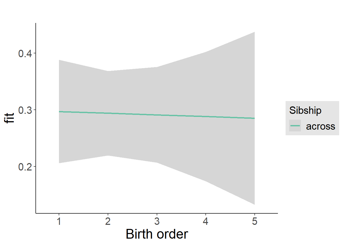
Add Birth Order Factor
Model Summary
m3_birthorder_nonlinear = update(m1_covariates_only, formula = . ~ . + birth_order_nonlinear)
tidy(m3_birthorder_nonlinear, conf.int = T, conf.level = 0.995)| effect | group | term | estimate | std.error | statistic | df | p.value | conf.low | conf.high |
|---|---|---|---|---|---|---|---|---|---|
| fixed | NA | (Intercept) | -1 | 4.399 | -0.2274 | 2131 | 0.8202 | -13.35 | 11.35 |
| fixed | NA | poly(age, 3, raw = TRUE)1 | 0.1247 | 0.4605 | 0.2708 | 2129 | 0.7865 | -1.168 | 1.417 |
| fixed | NA | poly(age, 3, raw = TRUE)2 | -0.003704 | 0.01584 | -0.2339 | 2127 | 0.8151 | -0.04816 | 0.04075 |
| fixed | NA | poly(age, 3, raw = TRUE)3 | 0.00003432 | 0.000179 | 0.1917 | 2125 | 0.848 | -0.0004682 | 0.0005369 |
| fixed | NA | male | 0.05993 | 0.03386 | 1.77 | 2207 | 0.07685 | -0.03511 | 0.155 |
| fixed | NA | sibling_count3 | -0.04035 | 0.05475 | -0.7369 | 1734 | 0.4613 | -0.194 | 0.1133 |
| fixed | NA | sibling_count4 | -0.07136 | 0.05745 | -1.242 | 1692 | 0.2143 | -0.2326 | 0.0899 |
| fixed | NA | sibling_count5 | -0.1478 | 0.0629 | -2.35 | 1720 | 0.01889 | -0.3244 | 0.02875 |
| fixed | NA | birth_order_nonlinear2 | -0.01205 | 0.04037 | -0.2986 | 1812 | 0.7653 | -0.1254 | 0.1013 |
| fixed | NA | birth_order_nonlinear3 | -0.02193 | 0.04916 | -0.4461 | 1968 | 0.6555 | -0.1599 | 0.1161 |
| fixed | NA | birth_order_nonlinear4 | -0.02862 | 0.06498 | -0.4405 | 2117 | 0.6596 | -0.211 | 0.1538 |
| fixed | NA | birth_order_nonlinear5 | 0.0424 | 0.09357 | 0.4532 | 2096 | 0.6505 | -0.2203 | 0.3051 |
| ran_pars | mother_pidlink | sd__(Intercept) | 0.3834 | NA | NA | NA | NA | NA | NA |
| ran_pars | Residual | sd__Observation | 0.7359 | NA | NA | NA | NA | NA | NA |
Coefficient Plot
plot_birthorder(m3_birthorder_nonlinear, separate = FALSE)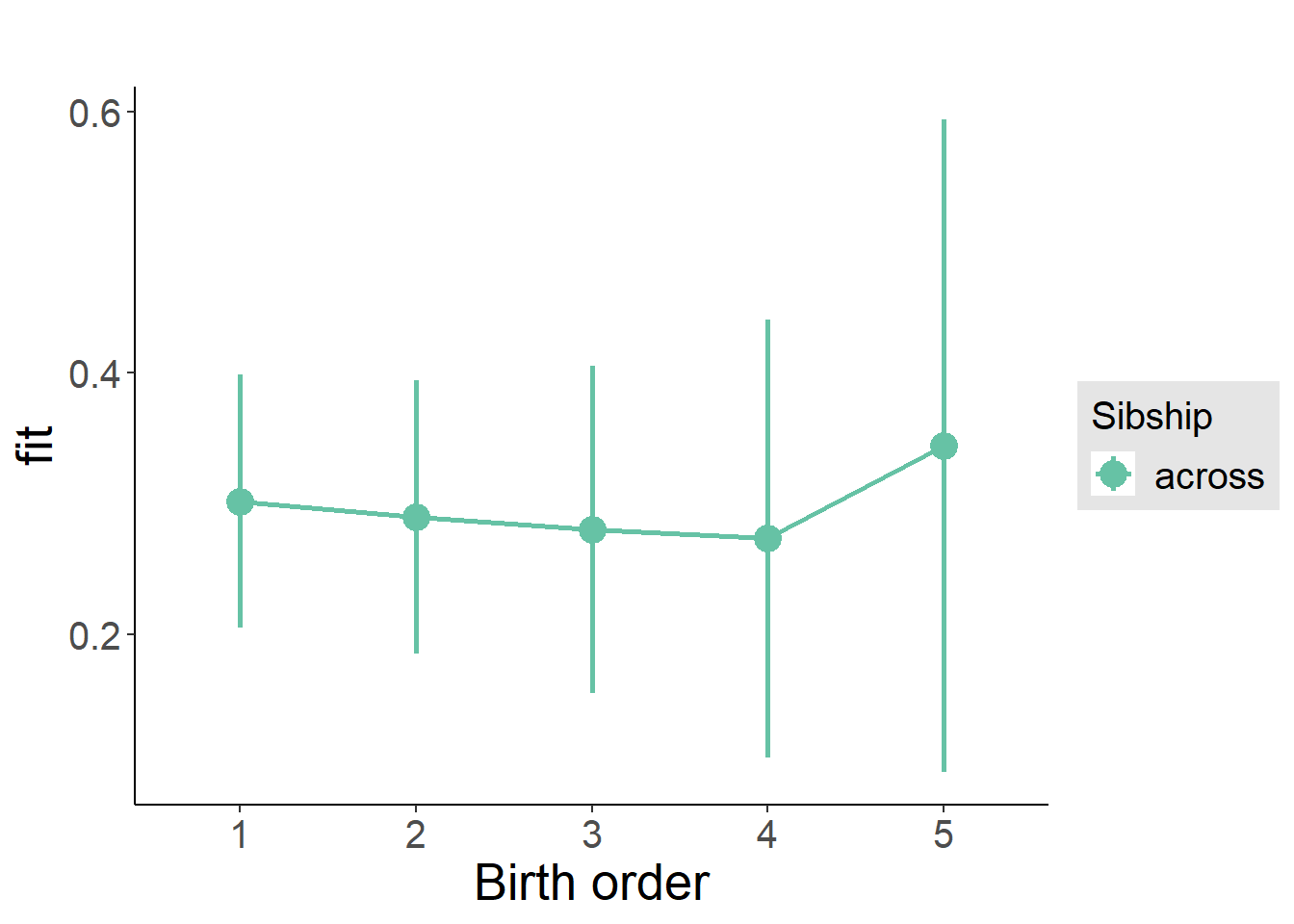
Add Interaction
Model Summary
m4_interaction = update(m3_birthorder_nonlinear, formula = . ~ . - birth_order_nonlinear - sibling_count + count_birth_order)
tidy(m4_interaction, conf.int = T, conf.level = 0.995)| effect | group | term | estimate | std.error | statistic | df | p.value | conf.low | conf.high |
|---|---|---|---|---|---|---|---|---|---|
| fixed | NA | (Intercept) | -1.186 | 4.409 | -0.2691 | 2124 | 0.7879 | -13.56 | 11.19 |
| fixed | NA | poly(age, 3, raw = TRUE)1 | 0.1455 | 0.4615 | 0.3153 | 2122 | 0.7526 | -1.15 | 1.441 |
| fixed | NA | poly(age, 3, raw = TRUE)2 | -0.004506 | 0.01587 | -0.2839 | 2120 | 0.7765 | -0.04905 | 0.04004 |
| fixed | NA | poly(age, 3, raw = TRUE)3 | 0.00004434 | 0.0001794 | 0.2472 | 2118 | 0.8048 | -0.0004592 | 0.0005479 |
| fixed | NA | male | 0.06036 | 0.03392 | 1.78 | 2202 | 0.07529 | -0.03485 | 0.1556 |
| fixed | NA | count_birth_order2/2 | 0.01977 | 0.07753 | 0.255 | 1772 | 0.7988 | -0.1979 | 0.2374 |
| fixed | NA | count_birth_order1/3 | -0.05247 | 0.0695 | -0.7549 | 2288 | 0.4504 | -0.2476 | 0.1426 |
| fixed | NA | count_birth_order2/3 | 0.007776 | 0.07558 | 0.1029 | 2302 | 0.9181 | -0.2044 | 0.2199 |
| fixed | NA | count_birth_order3/3 | -0.06859 | 0.08225 | -0.834 | 2301 | 0.4044 | -0.2995 | 0.1623 |
| fixed | NA | count_birth_order1/4 | -0.01434 | 0.07735 | -0.1854 | 2297 | 0.8529 | -0.2315 | 0.2028 |
| fixed | NA | count_birth_order2/4 | -0.1156 | 0.07821 | -1.478 | 2302 | 0.1396 | -0.3351 | 0.104 |
| fixed | NA | count_birth_order3/4 | -0.1448 | 0.08259 | -1.753 | 2291 | 0.07979 | -0.3766 | 0.08708 |
| fixed | NA | count_birth_order4/4 | -0.01648 | 0.09095 | -0.1812 | 2293 | 0.8562 | -0.2718 | 0.2388 |
| fixed | NA | count_birth_order1/5 | -0.128 | 0.08888 | -1.441 | 2302 | 0.1498 | -0.3775 | 0.1214 |
| fixed | NA | count_birth_order2/5 | -0.1972 | 0.09233 | -2.136 | 2296 | 0.03276 | -0.4564 | 0.06194 |
| fixed | NA | count_birth_order3/5 | -0.04265 | 0.09233 | -0.462 | 2278 | 0.6441 | -0.3018 | 0.2165 |
| fixed | NA | count_birth_order4/5 | -0.2416 | 0.09246 | -2.613 | 2278 | 0.009025 | -0.5012 | 0.01791 |
| fixed | NA | count_birth_order5/5 | -0.09316 | 0.09606 | -0.9698 | 2285 | 0.3322 | -0.3628 | 0.1765 |
| ran_pars | mother_pidlink | sd__(Intercept) | 0.384 | NA | NA | NA | NA | NA | NA |
| ran_pars | Residual | sd__Observation | 0.7351 | NA | NA | NA | NA | NA | NA |
Coefficient Plot
plot_birthorder(m4_interaction)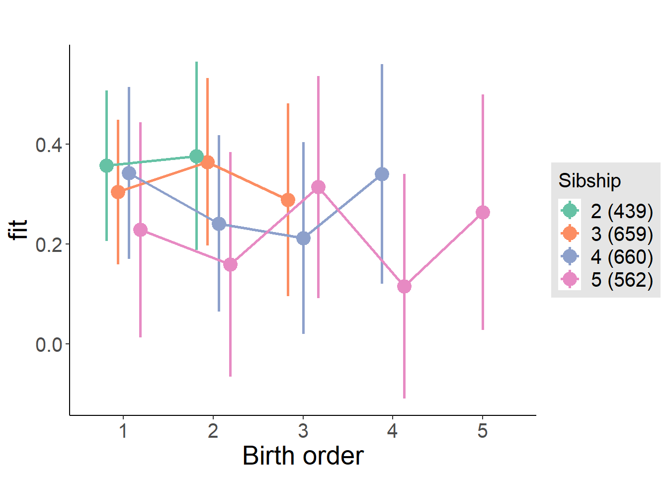
Model Comparison
###### Model 1 - Model 2
anova(m1_covariates_only, m2_birthorder_linear, m3_birthorder_nonlinear, m4_interaction)## refitting model(s) with ML (instead of REML)| Df | AIC | BIC | logLik | deviance | Chisq | Chi Df | Pr(>Chisq) |
|---|---|---|---|---|---|---|---|
| 10 | 5688 | 5745 | -2834 | 5668 | NA | NA | NA |
| 11 | 5690 | 5753 | -2834 | 5668 | 0.03242 | 1 | 0.8571 |
| 14 | 5695 | 5776 | -2834 | 5667 | 0.7083 | 3 | 0.8713 |
| 20 | 5699 | 5814 | -2829 | 5659 | 8.526 | 6 | 0.202 |
Parental full sibling order
outcome_parental_m1 <- update(m2_birthorder_linear, data = birthorder %>%
mutate(sibling_count = sibling_count_genes_factor,
birth_order_nonlinear = birthorder_genes_factor,
birth_order = birthorder_genes,
count_birth_order = count_birthorder_genes
) %>%
filter(sibling_count != "1"))
compare_models_markdown(outcome_parental_m1)Basic Model
Model Summary
m1_covariates_only <- update(m2_birthorder_linear, formula = . ~ . - birth_order)
tidy(m1_covariates_only, conf.int = T, conf.level = 0.995)| effect | group | term | estimate | std.error | statistic | df | p.value | conf.low | conf.high |
|---|---|---|---|---|---|---|---|---|---|
| fixed | NA | (Intercept) | -5.359 | 4.191 | -1.279 | 2335 | 0.2011 | -17.12 | 6.406 |
| fixed | NA | poly(age, 3, raw = TRUE)1 | 0.588 | 0.438 | 1.342 | 2334 | 0.1796 | -0.6414 | 1.817 |
| fixed | NA | poly(age, 3, raw = TRUE)2 | -0.01994 | 0.01504 | -1.326 | 2333 | 0.185 | -0.06214 | 0.02227 |
| fixed | NA | poly(age, 3, raw = TRUE)3 | 0.0002205 | 0.0001697 | 1.3 | 2330 | 0.1938 | -0.0002557 | 0.0006967 |
| fixed | NA | male | 0.05559 | 0.03248 | 1.711 | 2441 | 0.08715 | -0.03559 | 0.1468 |
| fixed | NA | sibling_count3 | -0.002478 | 0.04838 | -0.05122 | 1784 | 0.9592 | -0.1383 | 0.1333 |
| fixed | NA | sibling_count4 | -0.08207 | 0.05026 | -1.633 | 1691 | 0.1027 | -0.2232 | 0.05901 |
| fixed | NA | sibling_count5 | -0.1536 | 0.05614 | -2.736 | 1565 | 0.006295 | -0.3112 | 0.004005 |
| ran_pars | mother_pidlink | sd__(Intercept) | 0.4022 | NA | NA | NA | NA | NA | NA |
| ran_pars | Residual | sd__Observation | 0.735 | NA | NA | NA | NA | NA | NA |
Coefficient Plot
plot(allEffects(m1_covariates_only, confidence.level = 0.995))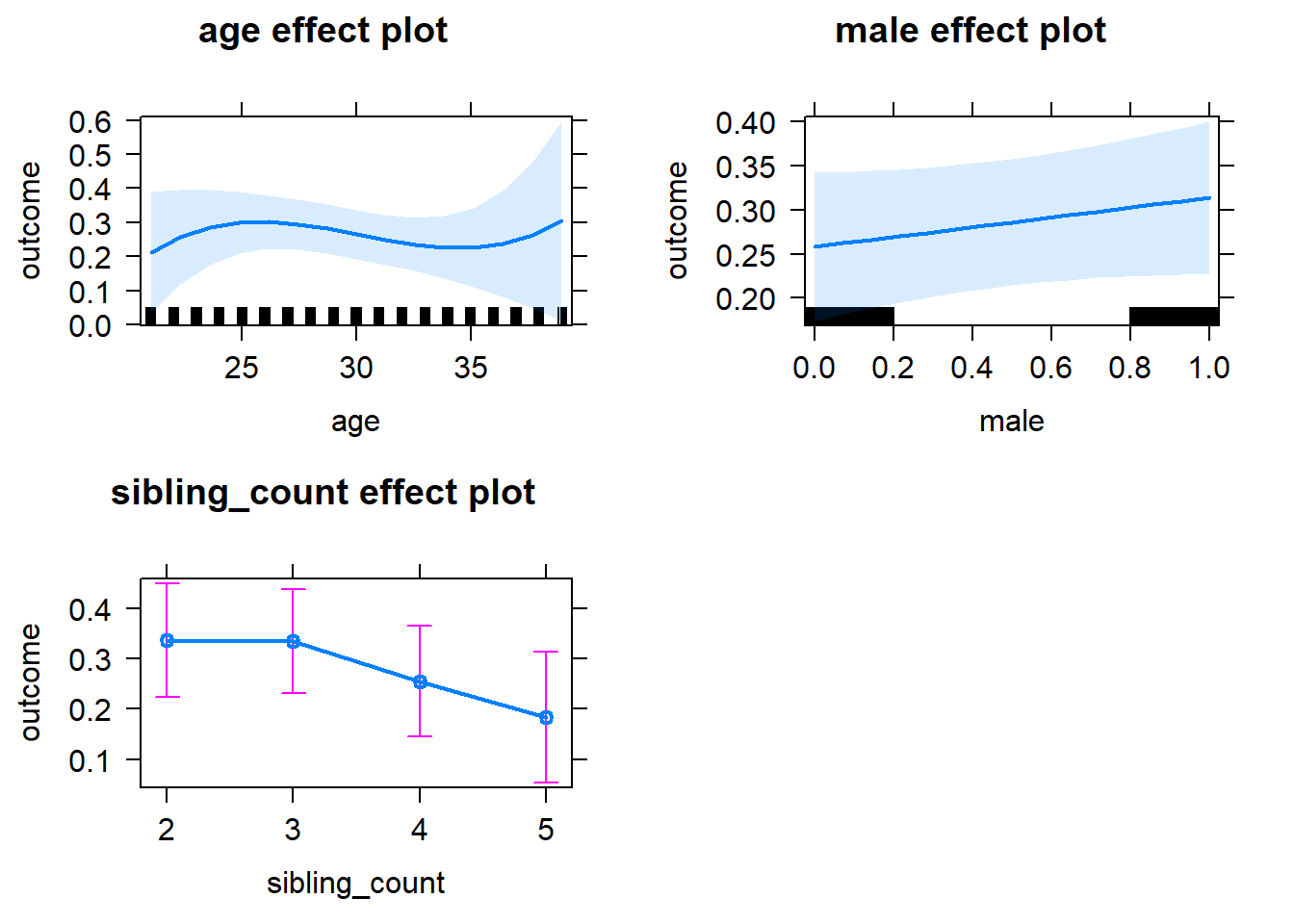
Add Birth Order Linear
Model Summary
tidy(m2_birthorder_linear, conf.int = T, conf.level = 0.995)| effect | group | term | estimate | std.error | statistic | df | p.value | conf.low | conf.high |
|---|---|---|---|---|---|---|---|---|---|
| fixed | NA | (Intercept) | -5.508 | 4.192 | -1.314 | 2335 | 0.1891 | -17.28 | 6.26 |
| fixed | NA | birth_order | 0.01995 | 0.01668 | 1.196 | 2458 | 0.2317 | -0.02686 | 0.06677 |
| fixed | NA | poly(age, 3, raw = TRUE)1 | 0.6008 | 0.438 | 1.372 | 2333 | 0.1703 | -0.6287 | 1.83 |
| fixed | NA | poly(age, 3, raw = TRUE)2 | -0.02041 | 0.01504 | -1.357 | 2331 | 0.1749 | -0.06262 | 0.0218 |
| fixed | NA | poly(age, 3, raw = TRUE)3 | 0.0002264 | 0.0001697 | 1.334 | 2329 | 0.1822 | -0.0002499 | 0.0007028 |
| fixed | NA | male | 0.0552 | 0.03248 | 1.7 | 2440 | 0.08934 | -0.03597 | 0.1464 |
| fixed | NA | sibling_count3 | -0.011 | 0.04891 | -0.2249 | 1804 | 0.8221 | -0.1483 | 0.1263 |
| fixed | NA | sibling_count4 | -0.1034 | 0.05333 | -1.938 | 1772 | 0.05277 | -0.253 | 0.04634 |
| fixed | NA | sibling_count5 | -0.1873 | 0.0628 | -2.982 | 1785 | 0.002906 | -0.3635 | -0.01097 |
| ran_pars | mother_pidlink | sd__(Intercept) | 0.4031 | NA | NA | NA | NA | NA | NA |
| ran_pars | Residual | sd__Observation | 0.7345 | NA | NA | NA | NA | NA | NA |
Coefficient Plot
plot_birthorder2(m2_birthorder_linear, separate = FALSE)
Add Birth Order Factor
Model Summary
m3_birthorder_nonlinear = update(m1_covariates_only, formula = . ~ . + birth_order_nonlinear)
tidy(m3_birthorder_nonlinear, conf.int = T, conf.level = 0.995)| effect | group | term | estimate | std.error | statistic | df | p.value | conf.low | conf.high |
|---|---|---|---|---|---|---|---|---|---|
| fixed | NA | (Intercept) | -5.571 | 4.194 | -1.328 | 2330 | 0.1842 | -17.35 | 6.203 |
| fixed | NA | poly(age, 3, raw = TRUE)1 | 0.6117 | 0.4383 | 1.396 | 2328 | 0.1629 | -0.6186 | 1.842 |
| fixed | NA | poly(age, 3, raw = TRUE)2 | -0.02081 | 0.01505 | -1.383 | 2326 | 0.1668 | -0.06305 | 0.02143 |
| fixed | NA | poly(age, 3, raw = TRUE)3 | 0.0002312 | 0.0001698 | 1.362 | 2324 | 0.1734 | -0.0002454 | 0.0007079 |
| fixed | NA | male | 0.05476 | 0.03249 | 1.685 | 2437 | 0.09208 | -0.03645 | 0.146 |
| fixed | NA | sibling_count3 | -0.02073 | 0.04953 | -0.4186 | 1863 | 0.6756 | -0.1598 | 0.1183 |
| fixed | NA | sibling_count4 | -0.1062 | 0.05409 | -1.963 | 1827 | 0.04977 | -0.258 | 0.04564 |
| fixed | NA | sibling_count5 | -0.195 | 0.06367 | -3.063 | 1831 | 0.002223 | -0.3737 | -0.0163 |
| fixed | NA | birth_order_nonlinear2 | -0.01028 | 0.03825 | -0.2688 | 1916 | 0.7881 | -0.1177 | 0.09709 |
| fixed | NA | birth_order_nonlinear3 | 0.07328 | 0.0472 | 1.553 | 2099 | 0.1206 | -0.0592 | 0.2058 |
| fixed | NA | birth_order_nonlinear4 | 0.01959 | 0.06336 | 0.3092 | 2337 | 0.7572 | -0.1583 | 0.1974 |
| fixed | NA | birth_order_nonlinear5 | 0.1004 | 0.1008 | 0.9956 | 2234 | 0.3195 | -0.1827 | 0.3834 |
| ran_pars | mother_pidlink | sd__(Intercept) | 0.4038 | NA | NA | NA | NA | NA | NA |
| ran_pars | Residual | sd__Observation | 0.7343 | NA | NA | NA | NA | NA | NA |
Coefficient Plot
plot_birthorder(m3_birthorder_nonlinear, separate = FALSE)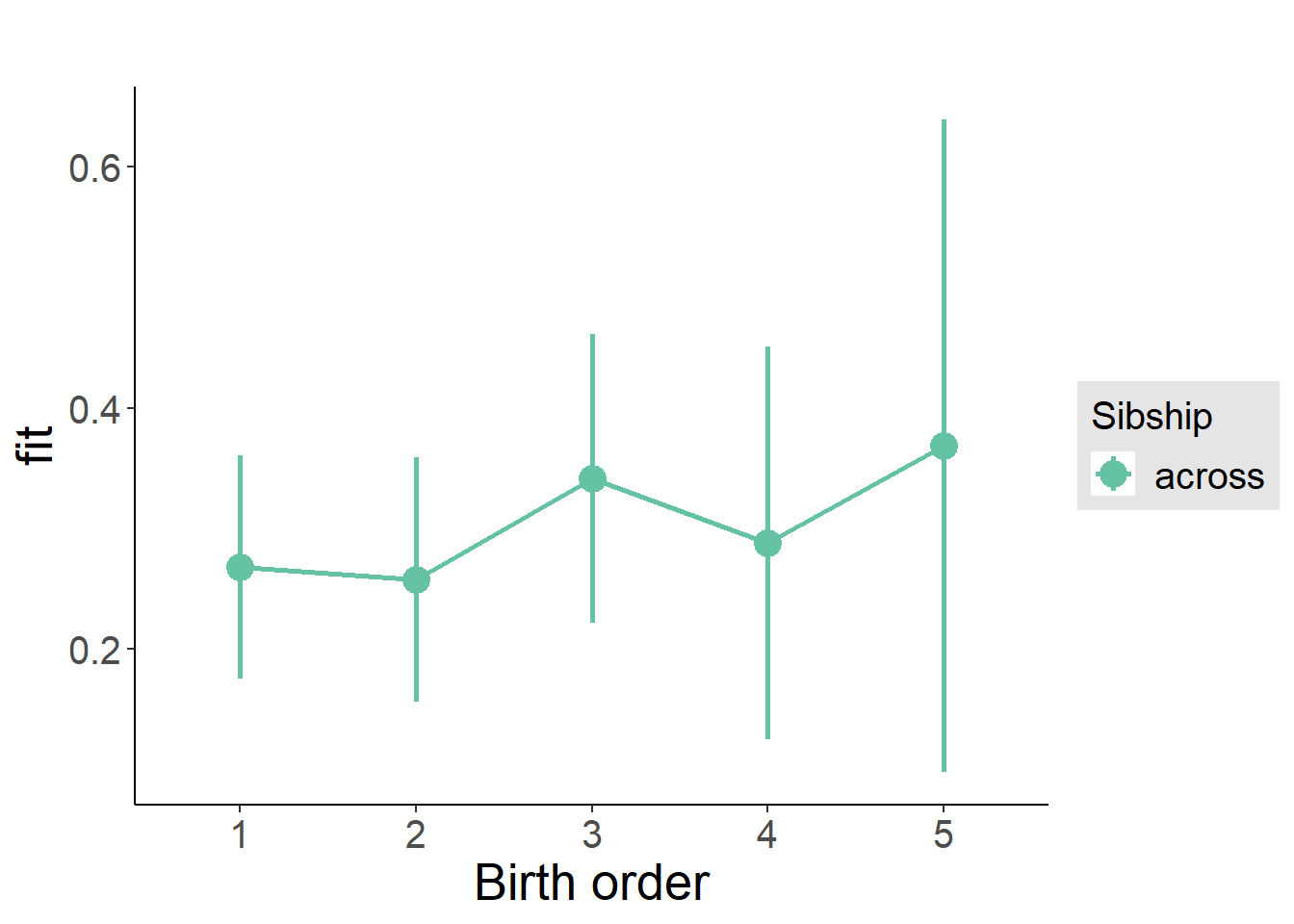
Add Interaction
Model Summary
m4_interaction = update(m3_birthorder_nonlinear, formula = . ~ . - birth_order_nonlinear - sibling_count + count_birth_order)
tidy(m4_interaction, conf.int = T, conf.level = 0.995)| effect | group | term | estimate | std.error | statistic | df | p.value | conf.low | conf.high |
|---|---|---|---|---|---|---|---|---|---|
| fixed | NA | (Intercept) | -5.506 | 4.192 | -1.313 | 2320 | 0.1892 | -17.27 | 6.262 |
| fixed | NA | poly(age, 3, raw = TRUE)1 | 0.6092 | 0.4381 | 1.391 | 2318 | 0.1645 | -0.6205 | 1.839 |
| fixed | NA | poly(age, 3, raw = TRUE)2 | -0.02082 | 0.01504 | -1.384 | 2316 | 0.1665 | -0.06304 | 0.0214 |
| fixed | NA | poly(age, 3, raw = TRUE)3 | 0.0002324 | 0.0001697 | 1.369 | 2314 | 0.1711 | -0.000244 | 0.0007088 |
| fixed | NA | male | 0.05624 | 0.03253 | 1.729 | 2431 | 0.08394 | -0.03507 | 0.1475 |
| fixed | NA | count_birth_order2/2 | -0.0546 | 0.06678 | -0.8176 | 1928 | 0.4137 | -0.242 | 0.1328 |
| fixed | NA | count_birth_order1/3 | -0.04933 | 0.06221 | -0.793 | 2518 | 0.4278 | -0.2239 | 0.1253 |
| fixed | NA | count_birth_order2/3 | 0.01169 | 0.06885 | 0.1697 | 2539 | 0.8652 | -0.1816 | 0.205 |
| fixed | NA | count_birth_order3/3 | -0.01606 | 0.07471 | -0.215 | 2535 | 0.8298 | -0.2258 | 0.1937 |
| fixed | NA | count_birth_order1/4 | -0.1051 | 0.07346 | -1.43 | 2535 | 0.1528 | -0.3113 | 0.1011 |
| fixed | NA | count_birth_order2/4 | -0.132 | 0.07501 | -1.76 | 2536 | 0.07857 | -0.3425 | 0.07855 |
| fixed | NA | count_birth_order3/4 | -0.1016 | 0.07622 | -1.333 | 2528 | 0.1828 | -0.3155 | 0.1124 |
| fixed | NA | count_birth_order4/4 | -0.06905 | 0.08164 | -0.8458 | 2535 | 0.3977 | -0.2982 | 0.1601 |
| fixed | NA | count_birth_order1/5 | -0.2639 | 0.09434 | -2.797 | 2537 | 0.005193 | -0.5287 | 0.0009223 |
| fixed | NA | count_birth_order2/5 | -0.3259 | 0.09988 | -3.263 | 2511 | 0.001117 | -0.6063 | -0.04555 |
| fixed | NA | count_birth_order3/5 | 0.03848 | 0.09108 | 0.4224 | 2510 | 0.6727 | -0.2172 | 0.2941 |
| fixed | NA | count_birth_order4/5 | -0.235 | 0.09142 | -2.57 | 2514 | 0.01022 | -0.4916 | 0.02165 |
| fixed | NA | count_birth_order5/5 | -0.1072 | 0.0992 | -1.081 | 2506 | 0.28 | -0.3856 | 0.1713 |
| ran_pars | mother_pidlink | sd__(Intercept) | 0.4064 | NA | NA | NA | NA | NA | NA |
| ran_pars | Residual | sd__Observation | 0.7321 | NA | NA | NA | NA | NA | NA |
Coefficient Plot
plot_birthorder(m4_interaction)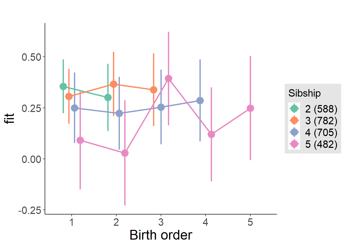
Model Comparison
###### Model 1 - Model 2
anova(m1_covariates_only, m2_birthorder_linear, m3_birthorder_nonlinear, m4_interaction)## refitting model(s) with ML (instead of REML)| Df | AIC | BIC | logLik | deviance | Chisq | Chi Df | Pr(>Chisq) |
|---|---|---|---|---|---|---|---|
| 10 | 6312 | 6370 | -3146 | 6292 | NA | NA | NA |
| 11 | 6312 | 6376 | -3145 | 6290 | 1.432 | 1 | 0.2314 |
| 14 | 6316 | 6398 | -3144 | 6288 | 2.444 | 3 | 0.4855 |
| 20 | 6316 | 6433 | -3138 | 6276 | 11.6 | 6 | 0.07141 |
Compare birth order specifications
library(coefplot)
multiplot(outcome_naive_m1, outcome_preg_m1, outcome_uterus_m1, outcome_parental_m1, dodgeHeight = 0.6,
intercept = FALSE)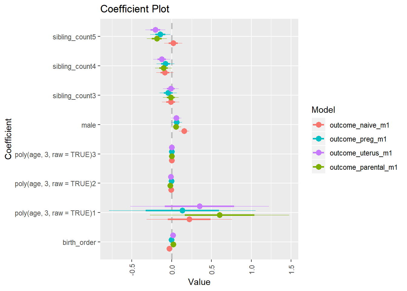
Numeracy 2007 old
birthorder <- birthorder %>% mutate(outcome = math_2007_old)
model = lmer(outcome ~ birth_order + poly(age, 3, raw = TRUE) + male + sibling_count + (1 | mother_pidlink),
data = birthorder)
compare_birthorder_specs(model)Naive birth order
outcome_naive_m1 <- update(m2_birthorder_linear, data = birthorder %>%
mutate(sibling_count = sibling_count_naive_factor,
birth_order_nonlinear = birthorder_naive_factor,
birth_order = birthorder_naive,
count_birth_order = count_birthorder_naive) %>%
filter(sibling_count != "1"))
compare_models_markdown(outcome_naive_m1)Basic Model
Model Summary
m1_covariates_only <- update(m2_birthorder_linear, formula = . ~ . - birth_order)
tidy(m1_covariates_only, conf.int = T, conf.level = 0.995)| effect | group | term | estimate | std.error | statistic | df | p.value | conf.low | conf.high |
|---|---|---|---|---|---|---|---|---|---|
| fixed | NA | (Intercept) | -4.457 | 2.732 | -1.632 | 3255 | 0.1028 | -12.13 | 3.211 |
| fixed | NA | poly(age, 3, raw = TRUE)1 | 0.5424 | 0.2859 | 1.897 | 3256 | 0.05791 | -0.2602 | 1.345 |
| fixed | NA | poly(age, 3, raw = TRUE)2 | -0.01929 | 0.009854 | -1.958 | 3258 | 0.05034 | -0.04695 | 0.008368 |
| fixed | NA | poly(age, 3, raw = TRUE)3 | 0.000212 | 0.0001118 | 1.897 | 3259 | 0.05788 | -0.0001017 | 0.0005258 |
| fixed | NA | male | -0.1061 | 0.03366 | -3.153 | 2996 | 0.001633 | -0.2006 | -0.01164 |
| fixed | NA | sibling_count3 | 0.03597 | 0.05849 | 0.615 | 2429 | 0.5386 | -0.1282 | 0.2002 |
| fixed | NA | sibling_count4 | -0.1177 | 0.05726 | -2.055 | 2339 | 0.03994 | -0.2784 | 0.04304 |
| fixed | NA | sibling_count5 | -0.05071 | 0.05826 | -0.8704 | 2204 | 0.3842 | -0.2142 | 0.1128 |
| ran_pars | mother_pidlink | sd__(Intercept) | 0.584 | NA | NA | NA | NA | NA | NA |
| ran_pars | Residual | sd__Observation | 0.8178 | NA | NA | NA | NA | NA | NA |
Coefficient Plot
plot(allEffects(m1_covariates_only, confidence.level = 0.995))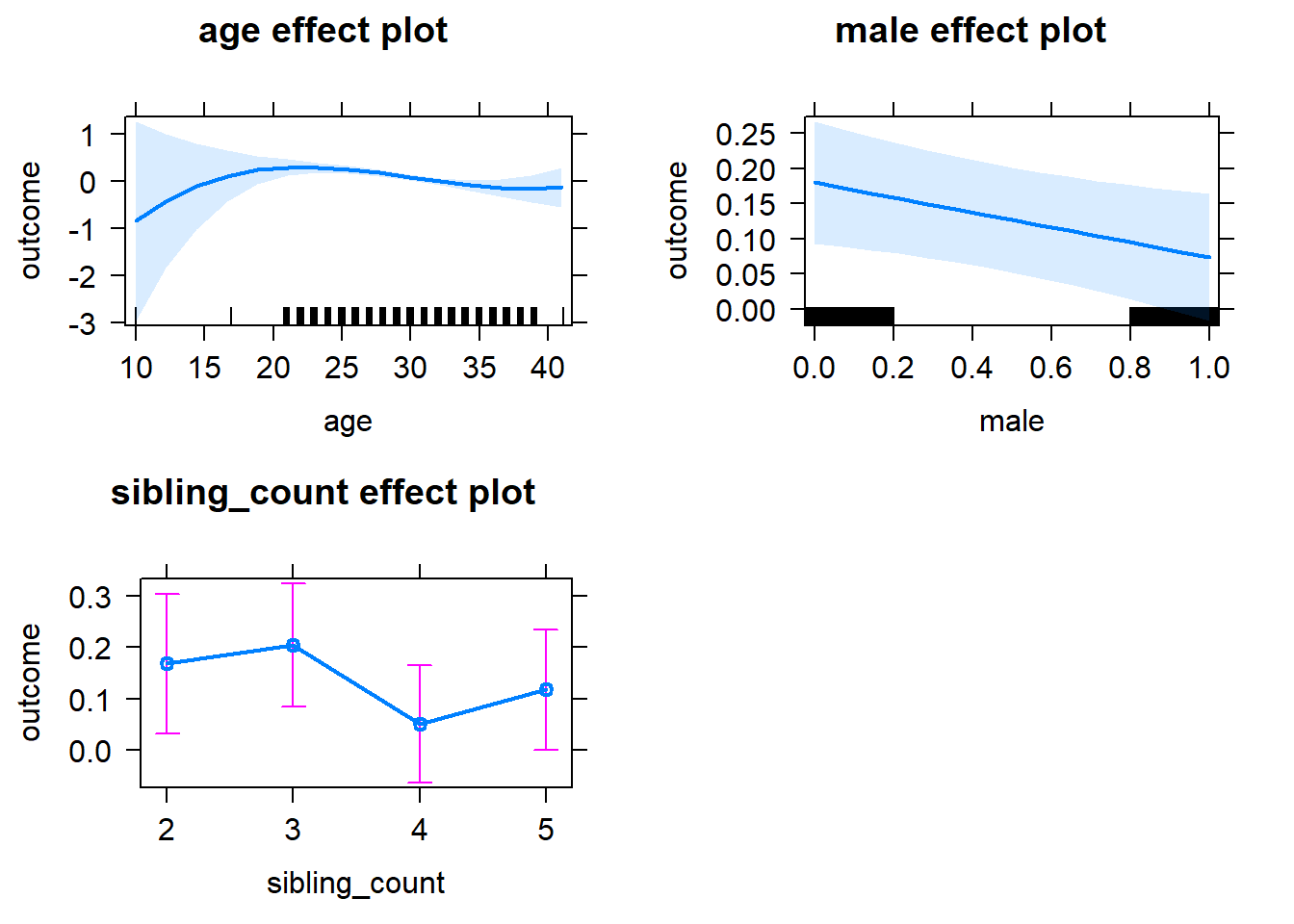
Add Birth Order Linear
Model Summary
tidy(m2_birthorder_linear, conf.int = T, conf.level = 0.995)| effect | group | term | estimate | std.error | statistic | df | p.value | conf.low | conf.high |
|---|---|---|---|---|---|---|---|---|---|
| fixed | NA | (Intercept) | -4.468 | 2.734 | -1.634 | 3255 | 0.1023 | -12.14 | 3.206 |
| fixed | NA | birth_order | 0.001952 | 0.0154 | 0.1268 | 2906 | 0.8991 | -0.04128 | 0.04519 |
| fixed | NA | poly(age, 3, raw = TRUE)1 | 0.5432 | 0.286 | 1.899 | 3256 | 0.05768 | -0.2598 | 1.346 |
| fixed | NA | poly(age, 3, raw = TRUE)2 | -0.01932 | 0.009858 | -1.959 | 3257 | 0.05014 | -0.04699 | 0.008355 |
| fixed | NA | poly(age, 3, raw = TRUE)3 | 0.0002123 | 0.0001118 | 1.899 | 3258 | 0.05766 | -0.0001015 | 0.0005262 |
| fixed | NA | male | -0.1061 | 0.03367 | -3.152 | 2995 | 0.001636 | -0.2007 | -0.01163 |
| fixed | NA | sibling_count3 | 0.03511 | 0.0589 | 0.596 | 2461 | 0.5512 | -0.1302 | 0.2005 |
| fixed | NA | sibling_count4 | -0.1195 | 0.05896 | -2.026 | 2468 | 0.04284 | -0.285 | 0.04603 |
| fixed | NA | sibling_count5 | -0.05356 | 0.06243 | -0.8578 | 2494 | 0.3911 | -0.2288 | 0.1217 |
| ran_pars | mother_pidlink | sd__(Intercept) | 0.5838 | NA | NA | NA | NA | NA | NA |
| ran_pars | Residual | sd__Observation | 0.8181 | NA | NA | NA | NA | NA | NA |
Coefficient Plot
plot_birthorder2(m2_birthorder_linear, separate = FALSE)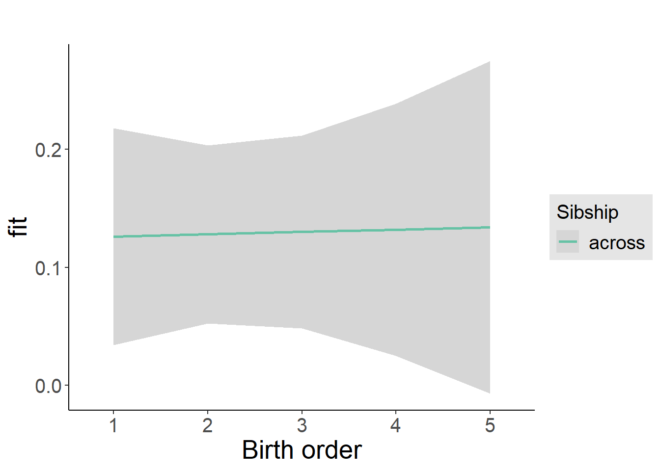
Add Birth Order Factor
Model Summary
m3_birthorder_nonlinear = update(m1_covariates_only, formula = . ~ . + birth_order_nonlinear)
tidy(m3_birthorder_nonlinear, conf.int = T, conf.level = 0.995)| effect | group | term | estimate | std.error | statistic | df | p.value | conf.low | conf.high |
|---|---|---|---|---|---|---|---|---|---|
| fixed | NA | (Intercept) | -4.267 | 2.737 | -1.559 | 3252 | 0.119 | -11.95 | 3.415 |
| fixed | NA | poly(age, 3, raw = TRUE)1 | 0.524 | 0.2864 | 1.83 | 3253 | 0.0674 | -0.2799 | 1.328 |
| fixed | NA | poly(age, 3, raw = TRUE)2 | -0.0187 | 0.009869 | -1.895 | 3254 | 0.05818 | -0.04641 | 0.009001 |
| fixed | NA | poly(age, 3, raw = TRUE)3 | 0.000206 | 0.0001119 | 1.841 | 3255 | 0.06577 | -0.0001082 | 0.0005202 |
| fixed | NA | male | -0.1053 | 0.03369 | -3.127 | 2995 | 0.001783 | -0.1999 | -0.01078 |
| fixed | NA | sibling_count3 | 0.04889 | 0.05991 | 0.8161 | 2546 | 0.4145 | -0.1193 | 0.2171 |
| fixed | NA | sibling_count4 | -0.1145 | 0.05981 | -1.914 | 2550 | 0.05573 | -0.2824 | 0.05341 |
| fixed | NA | sibling_count5 | -0.05681 | 0.06295 | -0.9026 | 2533 | 0.3668 | -0.2335 | 0.1199 |
| fixed | NA | birth_order_nonlinear2 | -0.01554 | 0.0409 | -0.38 | 2512 | 0.704 | -0.1304 | 0.09927 |
| fixed | NA | birth_order_nonlinear3 | -0.05006 | 0.04721 | -1.06 | 2500 | 0.289 | -0.1826 | 0.08245 |
| fixed | NA | birth_order_nonlinear4 | 0.02073 | 0.05856 | 0.3539 | 2658 | 0.7234 | -0.1436 | 0.1851 |
| fixed | NA | birth_order_nonlinear5 | 0.04748 | 0.08337 | 0.5695 | 2642 | 0.5691 | -0.1865 | 0.2815 |
| ran_pars | mother_pidlink | sd__(Intercept) | 0.5821 | NA | NA | NA | NA | NA | NA |
| ran_pars | Residual | sd__Observation | 0.8192 | NA | NA | NA | NA | NA | NA |
Coefficient Plot
plot_birthorder(m3_birthorder_nonlinear, separate = FALSE)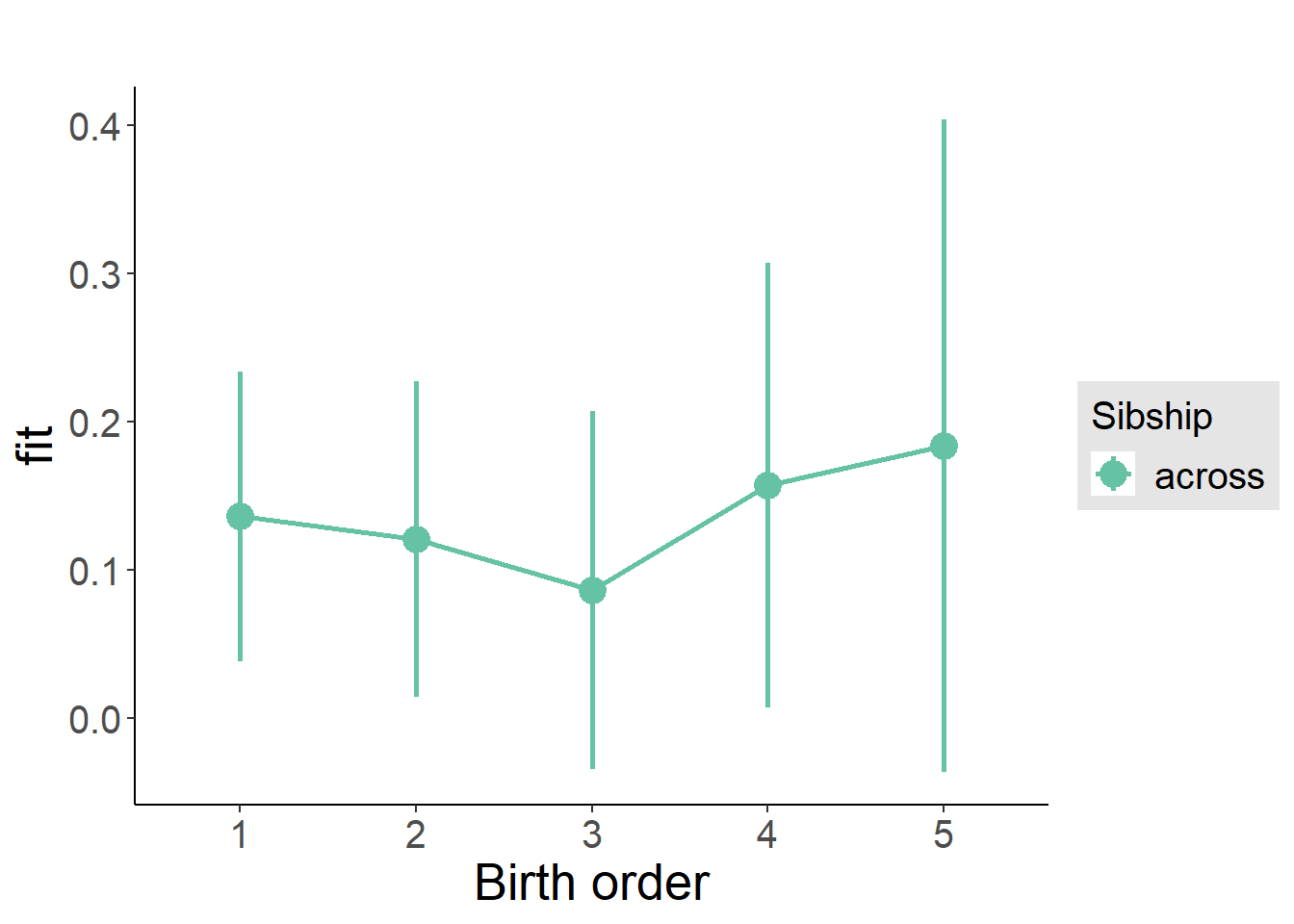
Add Interaction
Model Summary
m4_interaction = update(m3_birthorder_nonlinear, formula = . ~ . - birth_order_nonlinear - sibling_count + count_birth_order)
tidy(m4_interaction, conf.int = T, conf.level = 0.995)| effect | group | term | estimate | std.error | statistic | df | p.value | conf.low | conf.high |
|---|---|---|---|---|---|---|---|---|---|
| fixed | NA | (Intercept) | -4.415 | 2.741 | -1.611 | 3246 | 0.1073 | -12.11 | 3.279 |
| fixed | NA | poly(age, 3, raw = TRUE)1 | 0.5414 | 0.2868 | 1.887 | 3247 | 0.05918 | -0.2638 | 1.347 |
| fixed | NA | poly(age, 3, raw = TRUE)2 | -0.01927 | 0.009884 | -1.95 | 3248 | 0.05131 | -0.04702 | 0.008475 |
| fixed | NA | poly(age, 3, raw = TRUE)3 | 0.0002121 | 0.0001121 | 1.892 | 3249 | 0.05855 | -0.0001025 | 0.0005268 |
| fixed | NA | male | -0.1066 | 0.03373 | -3.161 | 2985 | 0.001588 | -0.2013 | -0.01194 |
| fixed | NA | count_birth_order2/2 | -0.0757 | 0.07771 | -0.9742 | 2592 | 0.3301 | -0.2938 | 0.1424 |
| fixed | NA | count_birth_order1/3 | 0.004212 | 0.07872 | 0.05351 | 3226 | 0.9573 | -0.2168 | 0.2252 |
| fixed | NA | count_birth_order2/3 | 0.04847 | 0.08393 | 0.5775 | 3249 | 0.5636 | -0.1871 | 0.2841 |
| fixed | NA | count_birth_order3/3 | -0.04386 | 0.08423 | -0.5207 | 3247 | 0.6026 | -0.2803 | 0.1926 |
| fixed | NA | count_birth_order1/4 | -0.1728 | 0.08107 | -2.132 | 3244 | 0.03308 | -0.4004 | 0.05472 |
| fixed | NA | count_birth_order2/4 | -0.1319 | 0.08437 | -1.564 | 3248 | 0.118 | -0.3688 | 0.1049 |
| fixed | NA | count_birth_order3/4 | -0.2138 | 0.08672 | -2.466 | 3235 | 0.01373 | -0.4572 | 0.0296 |
| fixed | NA | count_birth_order4/4 | -0.08364 | 0.08755 | -0.9553 | 3248 | 0.3395 | -0.3294 | 0.1621 |
| fixed | NA | count_birth_order1/5 | -0.0523 | 0.08876 | -0.5892 | 3245 | 0.5558 | -0.3015 | 0.1969 |
| fixed | NA | count_birth_order2/5 | -0.1417 | 0.09026 | -1.57 | 3235 | 0.1165 | -0.3951 | 0.1116 |
| fixed | NA | count_birth_order3/5 | -0.08611 | 0.08907 | -0.9668 | 3225 | 0.3337 | -0.3361 | 0.1639 |
| fixed | NA | count_birth_order4/5 | -0.1041 | 0.09102 | -1.144 | 3209 | 0.2528 | -0.3596 | 0.1514 |
| fixed | NA | count_birth_order5/5 | -0.037 | 0.09297 | -0.398 | 3233 | 0.6906 | -0.298 | 0.224 |
| ran_pars | mother_pidlink | sd__(Intercept) | 0.5833 | NA | NA | NA | NA | NA | NA |
| ran_pars | Residual | sd__Observation | 0.8189 | NA | NA | NA | NA | NA | NA |
Coefficient Plot
plot_birthorder(m4_interaction)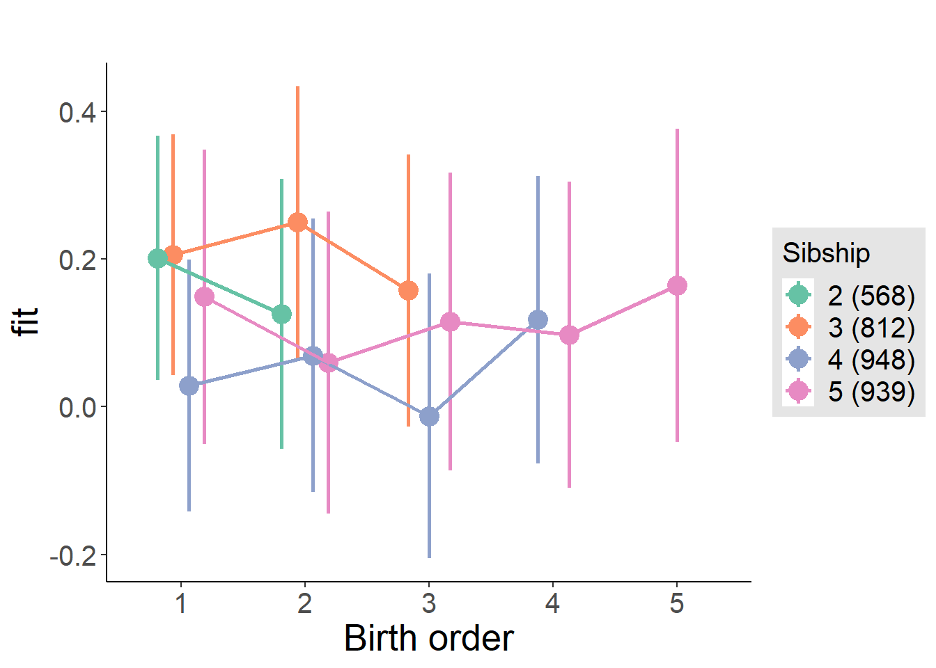
Model Comparison
###### Model 1 - Model 2
anova(m1_covariates_only, m2_birthorder_linear, m3_birthorder_nonlinear, m4_interaction)## refitting model(s) with ML (instead of REML)| Df | AIC | BIC | logLik | deviance | Chisq | Chi Df | Pr(>Chisq) |
|---|---|---|---|---|---|---|---|
| 10 | 9173 | 9234 | -4576 | 9153 | NA | NA | NA |
| 11 | 9175 | 9242 | -4576 | 9153 | 0.01638 | 1 | 0.8982 |
| 14 | 9179 | 9264 | -4575 | 9151 | 2.313 | 3 | 0.5101 |
| 20 | 9187 | 9309 | -4573 | 9147 | 3.815 | 6 | 0.7017 |
Maternal birth order
outcome_uterus_m1 <- update(m2_birthorder_linear, data = birthorder %>%
mutate(sibling_count = sibling_count_uterus_alive_factor,
birth_order_nonlinear = birthorder_uterus_alive_factor,
birth_order = birthorder_uterus_alive,
count_birth_order = count_birthorder_uterus_alive) %>%
filter(sibling_count != "1"))
compare_models_markdown(outcome_uterus_m1)Basic Model
Model Summary
m1_covariates_only <- update(m2_birthorder_linear, formula = . ~ . - birth_order)
tidy(m1_covariates_only, conf.int = T, conf.level = 0.995)| effect | group | term | estimate | std.error | statistic | df | p.value | conf.low | conf.high |
|---|---|---|---|---|---|---|---|---|---|
| fixed | NA | (Intercept) | -6.68 | 4.853 | -1.377 | 2238 | 0.1688 | -20.3 | 6.943 |
| fixed | NA | poly(age, 3, raw = TRUE)1 | 0.7869 | 0.5074 | 1.551 | 2234 | 0.1211 | -0.6374 | 2.211 |
| fixed | NA | poly(age, 3, raw = TRUE)2 | -0.0279 | 0.01743 | -1.601 | 2229 | 0.1096 | -0.07682 | 0.02102 |
| fixed | NA | poly(age, 3, raw = TRUE)3 | 0.0003159 | 0.0001968 | 1.606 | 2224 | 0.1085 | -0.0002364 | 0.0008682 |
| fixed | NA | male | -0.1556 | 0.03788 | -4.108 | 2350 | 0.00004132 | -0.2619 | -0.04927 |
| fixed | NA | sibling_count3 | 0.02745 | 0.0592 | 0.4636 | 1815 | 0.643 | -0.1387 | 0.1936 |
| fixed | NA | sibling_count4 | -0.04673 | 0.06138 | -0.7613 | 1741 | 0.4466 | -0.219 | 0.1256 |
| fixed | NA | sibling_count5 | -0.1241 | 0.06718 | -1.848 | 1690 | 0.0648 | -0.3127 | 0.06444 |
| ran_pars | mother_pidlink | sd__(Intercept) | 0.5604 | NA | NA | NA | NA | NA | NA |
| ran_pars | Residual | sd__Observation | 0.82 | NA | NA | NA | NA | NA | NA |
Coefficient Plot
plot(allEffects(m1_covariates_only, confidence.level = 0.995))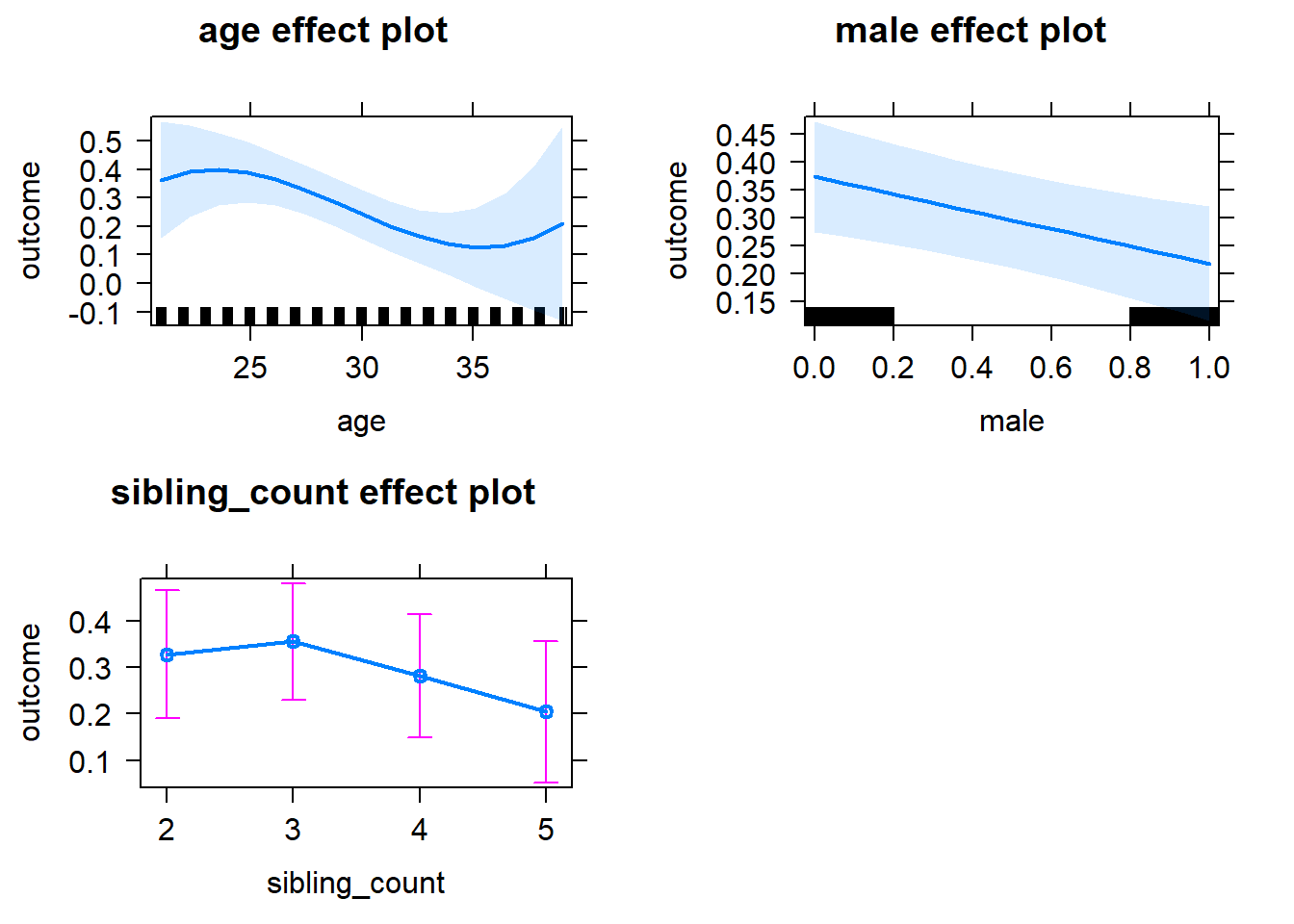
Add Birth Order Linear
Model Summary
tidy(m2_birthorder_linear, conf.int = T, conf.level = 0.995)| effect | group | term | estimate | std.error | statistic | df | p.value | conf.low | conf.high |
|---|---|---|---|---|---|---|---|---|---|
| fixed | NA | (Intercept) | -6.893 | 4.856 | -1.419 | 2239 | 0.1559 | -20.52 | 6.739 |
| fixed | NA | birth_order | 0.02361 | 0.01937 | 1.219 | 2449 | 0.2231 | -0.03077 | 0.07799 |
| fixed | NA | poly(age, 3, raw = TRUE)1 | 0.806 | 0.5076 | 1.588 | 2235 | 0.1125 | -0.6189 | 2.231 |
| fixed | NA | poly(age, 3, raw = TRUE)2 | -0.02859 | 0.01744 | -1.64 | 2230 | 0.1012 | -0.07754 | 0.02035 |
| fixed | NA | poly(age, 3, raw = TRUE)3 | 0.0003246 | 0.0001969 | 1.649 | 2225 | 0.09932 | -0.000228 | 0.0008772 |
| fixed | NA | male | -0.1559 | 0.03787 | -4.117 | 2349 | 0.00003965 | -0.2623 | -0.04963 |
| fixed | NA | sibling_count3 | 0.01752 | 0.05975 | 0.2933 | 1834 | 0.7693 | -0.1502 | 0.1852 |
| fixed | NA | sibling_count4 | -0.07218 | 0.06483 | -1.113 | 1809 | 0.2657 | -0.2542 | 0.1098 |
| fixed | NA | sibling_count5 | -0.1664 | 0.07558 | -2.201 | 1895 | 0.02785 | -0.3785 | 0.0458 |
| ran_pars | mother_pidlink | sd__(Intercept) | 0.5601 | NA | NA | NA | NA | NA | NA |
| ran_pars | Residual | sd__Observation | 0.8201 | NA | NA | NA | NA | NA | NA |
Coefficient Plot
plot_birthorder2(m2_birthorder_linear, separate = FALSE)
Add Birth Order Factor
Model Summary
m3_birthorder_nonlinear = update(m1_covariates_only, formula = . ~ . + birth_order_nonlinear)
tidy(m3_birthorder_nonlinear, conf.int = T, conf.level = 0.995)| effect | group | term | estimate | std.error | statistic | df | p.value | conf.low | conf.high |
|---|---|---|---|---|---|---|---|---|---|
| fixed | NA | (Intercept) | -6.836 | 4.856 | -1.408 | 2233 | 0.1594 | -20.47 | 6.795 |
| fixed | NA | poly(age, 3, raw = TRUE)1 | 0.8049 | 0.5077 | 1.585 | 2228 | 0.113 | -0.6202 | 2.23 |
| fixed | NA | poly(age, 3, raw = TRUE)2 | -0.02857 | 0.01744 | -1.639 | 2223 | 0.1014 | -0.07753 | 0.02038 |
| fixed | NA | poly(age, 3, raw = TRUE)3 | 0.0003247 | 0.0001969 | 1.649 | 2218 | 0.09926 | -0.000228 | 0.0008774 |
| fixed | NA | male | -0.1564 | 0.03787 | -4.131 | 2344 | 0.00003733 | -0.2627 | -0.05015 |
| fixed | NA | sibling_count3 | 0.01956 | 0.06035 | 0.3241 | 1881 | 0.7459 | -0.1498 | 0.189 |
| fixed | NA | sibling_count4 | -0.08656 | 0.06567 | -1.318 | 1858 | 0.1876 | -0.2709 | 0.09777 |
| fixed | NA | sibling_count5 | -0.1744 | 0.07646 | -2.281 | 1930 | 0.02266 | -0.389 | 0.04022 |
| fixed | NA | birth_order_nonlinear2 | -0.03023 | 0.04435 | -0.6816 | 1880 | 0.4956 | -0.1547 | 0.09426 |
| fixed | NA | birth_order_nonlinear3 | 0.02447 | 0.0549 | 0.4456 | 2070 | 0.6559 | -0.1297 | 0.1786 |
| fixed | NA | birth_order_nonlinear4 | 0.1414 | 0.07344 | 1.925 | 2298 | 0.05431 | -0.06475 | 0.3475 |
| fixed | NA | birth_order_nonlinear5 | 0.02823 | 0.11 | 0.2566 | 2207 | 0.7975 | -0.2806 | 0.3371 |
| ran_pars | mother_pidlink | sd__(Intercept) | 0.5617 | NA | NA | NA | NA | NA | NA |
| ran_pars | Residual | sd__Observation | 0.819 | NA | NA | NA | NA | NA | NA |
Coefficient Plot
plot_birthorder(m3_birthorder_nonlinear, separate = FALSE)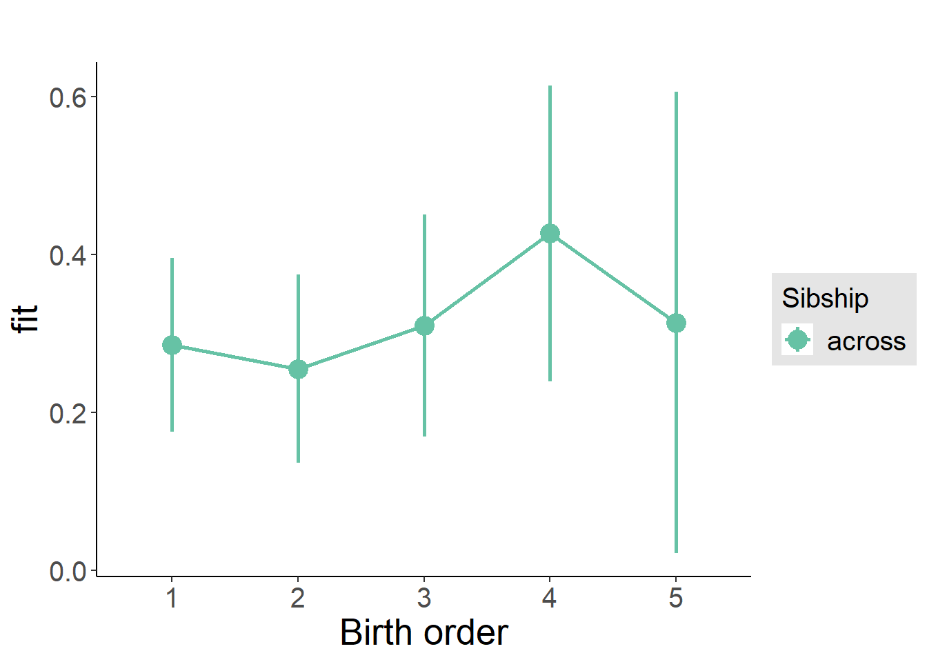
Add Interaction
Model Summary
m4_interaction = update(m3_birthorder_nonlinear, formula = . ~ . - birth_order_nonlinear - sibling_count + count_birth_order)
tidy(m4_interaction, conf.int = T, conf.level = 0.995)| effect | group | term | estimate | std.error | statistic | df | p.value | conf.low | conf.high |
|---|---|---|---|---|---|---|---|---|---|
| fixed | NA | (Intercept) | -6.779 | 4.858 | -1.395 | 2225 | 0.1631 | -20.42 | 6.859 |
| fixed | NA | poly(age, 3, raw = TRUE)1 | 0.8018 | 0.5079 | 1.579 | 2220 | 0.1146 | -0.6239 | 2.228 |
| fixed | NA | poly(age, 3, raw = TRUE)2 | -0.02847 | 0.01745 | -1.632 | 2215 | 0.1028 | -0.07745 | 0.0205 |
| fixed | NA | poly(age, 3, raw = TRUE)3 | 0.0003237 | 0.000197 | 1.643 | 2210 | 0.1005 | -0.0002292 | 0.0008766 |
| fixed | NA | male | -0.1605 | 0.03794 | -4.231 | 2341 | 0.0000242 | -0.267 | -0.05402 |
| fixed | NA | count_birth_order2/2 | -0.1024 | 0.07909 | -1.295 | 1884 | 0.1954 | -0.3244 | 0.1196 |
| fixed | NA | count_birth_order1/3 | -0.02307 | 0.07439 | -0.3101 | 2491 | 0.7565 | -0.2319 | 0.1857 |
| fixed | NA | count_birth_order2/3 | -0.02947 | 0.08131 | -0.3624 | 2526 | 0.717 | -0.2577 | 0.1988 |
| fixed | NA | count_birth_order3/3 | 0.04417 | 0.08999 | 0.4909 | 2524 | 0.6236 | -0.2084 | 0.2968 |
| fixed | NA | count_birth_order1/4 | -0.1308 | 0.08685 | -1.507 | 2520 | 0.132 | -0.3746 | 0.1129 |
| fixed | NA | count_birth_order2/4 | -0.0849 | 0.08843 | -0.96 | 2526 | 0.3371 | -0.3331 | 0.1633 |
| fixed | NA | count_birth_order3/4 | -0.1839 | 0.08946 | -2.056 | 2515 | 0.03993 | -0.435 | 0.06723 |
| fixed | NA | count_birth_order4/4 | 0.09668 | 0.09717 | 0.995 | 2520 | 0.3198 | -0.1761 | 0.3694 |
| fixed | NA | count_birth_order1/5 | -0.2013 | 0.112 | -1.798 | 2523 | 0.07236 | -0.5157 | 0.1131 |
| fixed | NA | count_birth_order2/5 | -0.2702 | 0.1156 | -2.337 | 2490 | 0.0195 | -0.5948 | 0.05431 |
| fixed | NA | count_birth_order3/5 | -0.05964 | 0.1052 | -0.5667 | 2488 | 0.571 | -0.3551 | 0.2358 |
| fixed | NA | count_birth_order4/5 | -0.1405 | 0.1046 | -1.343 | 2501 | 0.1793 | -0.4342 | 0.1531 |
| fixed | NA | count_birth_order5/5 | -0.1716 | 0.1095 | -1.568 | 2502 | 0.1171 | -0.4789 | 0.1357 |
| ran_pars | mother_pidlink | sd__(Intercept) | 0.5637 | NA | NA | NA | NA | NA | NA |
| ran_pars | Residual | sd__Observation | 0.8175 | NA | NA | NA | NA | NA | NA |
Coefficient Plot
plot_birthorder(m4_interaction)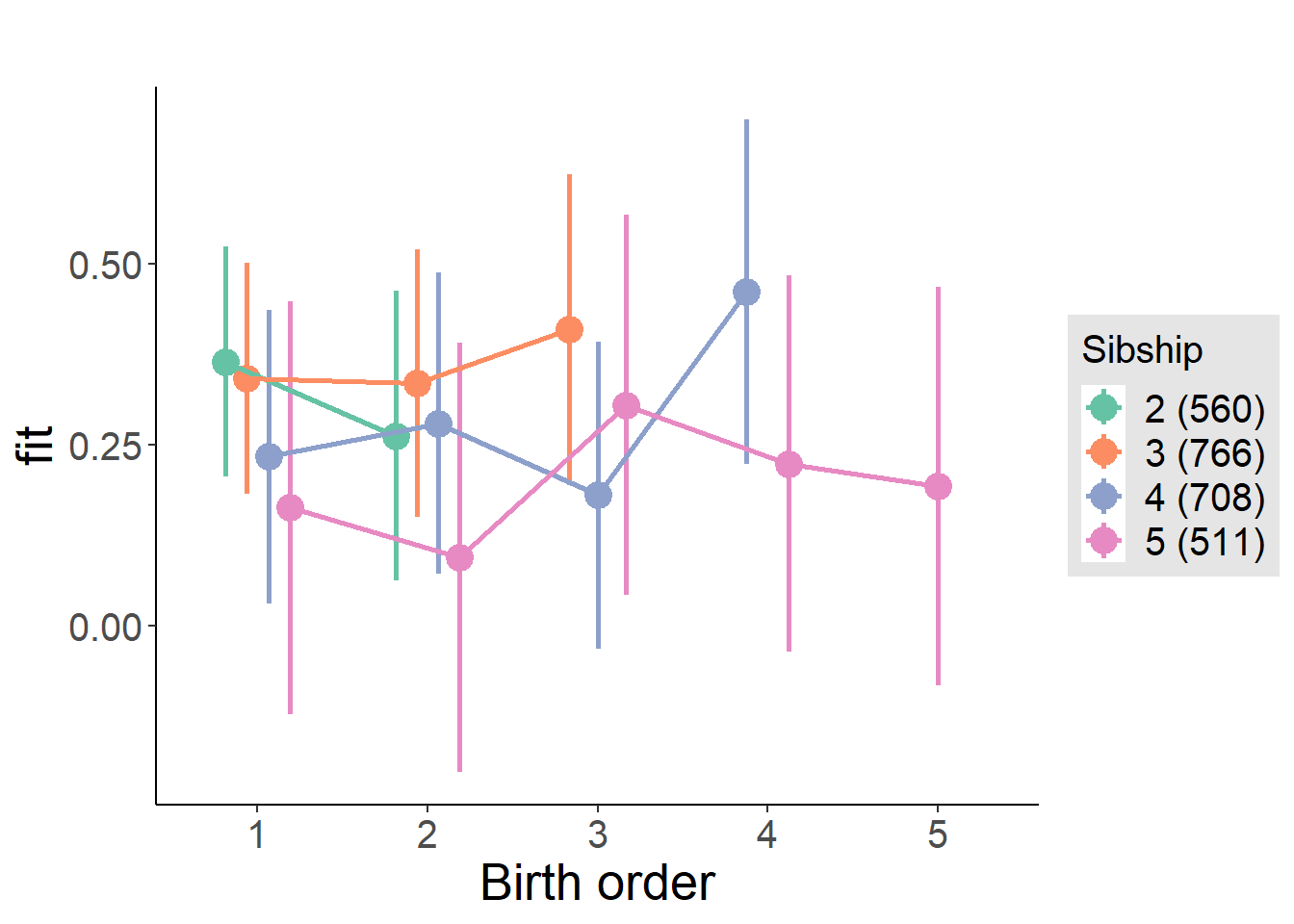
Model Comparison
###### Model 1 - Model 2
anova(m1_covariates_only, m2_birthorder_linear, m3_birthorder_nonlinear, m4_interaction)## refitting model(s) with ML (instead of REML)| Df | AIC | BIC | logLik | deviance | Chisq | Chi Df | Pr(>Chisq) |
|---|---|---|---|---|---|---|---|
| 10 | 7102 | 7161 | -3541 | 7082 | NA | NA | NA |
| 11 | 7103 | 7167 | -3540 | 7081 | 1.49 | 1 | 0.2222 |
| 14 | 7105 | 7187 | -3538 | 7077 | 4.061 | 3 | 0.255 |
| 20 | 7109 | 7226 | -3535 | 7069 | 7.837 | 6 | 0.2503 |
Maternal pregnancy order
outcome_preg_m1 <- update(m2_birthorder_linear, data = birthorder %>%
mutate(sibling_count = sibling_count_uterus_preg_factor,
birth_order_nonlinear = birthorder_uterus_preg_factor,
birth_order = birthorder_uterus_preg,
count_birth_order = count_birthorder_uterus_preg
) %>%
filter(sibling_count != "1"))
compare_models_markdown(outcome_preg_m1)Basic Model
Model Summary
m1_covariates_only <- update(m2_birthorder_linear, formula = . ~ . - birth_order)
tidy(m1_covariates_only, conf.int = T, conf.level = 0.995)| effect | group | term | estimate | std.error | statistic | df | p.value | conf.low | conf.high |
|---|---|---|---|---|---|---|---|---|---|
| fixed | NA | (Intercept) | -4.237 | 5.137 | -0.8248 | 2035 | 0.4096 | -18.66 | 10.18 |
| fixed | NA | poly(age, 3, raw = TRUE)1 | 0.5105 | 0.5377 | 0.9494 | 2031 | 0.3425 | -0.9989 | 2.02 |
| fixed | NA | poly(age, 3, raw = TRUE)2 | -0.01775 | 0.01849 | -0.9601 | 2028 | 0.3371 | -0.06966 | 0.03415 |
| fixed | NA | poly(age, 3, raw = TRUE)3 | 0.0001941 | 0.000209 | 0.929 | 2023 | 0.353 | -0.0003925 | 0.0007808 |
| fixed | NA | male | -0.1386 | 0.03971 | -3.49 | 2117 | 0.0004922 | -0.2501 | -0.02714 |
| fixed | NA | sibling_count3 | 0.0148 | 0.06556 | 0.2257 | 1686 | 0.8214 | -0.1692 | 0.1988 |
| fixed | NA | sibling_count4 | -0.0346 | 0.06664 | -0.5192 | 1633 | 0.6037 | -0.2217 | 0.1525 |
| fixed | NA | sibling_count5 | -0.05863 | 0.06953 | -0.8431 | 1594 | 0.3993 | -0.2538 | 0.1366 |
| ran_pars | mother_pidlink | sd__(Intercept) | 0.565 | NA | NA | NA | NA | NA | NA |
| ran_pars | Residual | sd__Observation | 0.8196 | NA | NA | NA | NA | NA | NA |
Coefficient Plot
plot(allEffects(m1_covariates_only, confidence.level = 0.995))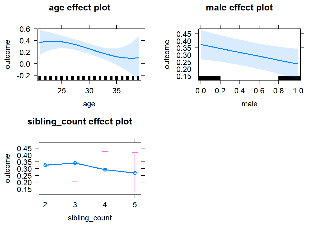
Add Birth Order Linear
Model Summary
tidy(m2_birthorder_linear, conf.int = T, conf.level = 0.995)| effect | group | term | estimate | std.error | statistic | df | p.value | conf.low | conf.high |
|---|---|---|---|---|---|---|---|---|---|
| fixed | NA | (Intercept) | -4.408 | 5.142 | -0.8573 | 2035 | 0.3914 | -18.84 | 10.03 |
| fixed | NA | birth_order | 0.01701 | 0.01964 | 0.8665 | 2242 | 0.3863 | -0.03811 | 0.07214 |
| fixed | NA | poly(age, 3, raw = TRUE)1 | 0.5261 | 0.5381 | 0.9776 | 2031 | 0.3284 | -0.9844 | 2.037 |
| fixed | NA | poly(age, 3, raw = TRUE)2 | -0.01831 | 0.01851 | -0.9896 | 2027 | 0.3225 | -0.07026 | 0.03363 |
| fixed | NA | poly(age, 3, raw = TRUE)3 | 0.000201 | 0.0002092 | 0.9612 | 2023 | 0.3366 | -0.0003861 | 0.0007882 |
| fixed | NA | male | -0.1384 | 0.03972 | -3.484 | 2117 | 0.0005045 | -0.2499 | -0.02688 |
| fixed | NA | sibling_count3 | 0.007267 | 0.06612 | 0.1099 | 1698 | 0.9125 | -0.1783 | 0.1929 |
| fixed | NA | sibling_count4 | -0.05148 | 0.06943 | -0.7414 | 1676 | 0.4585 | -0.2464 | 0.1434 |
| fixed | NA | sibling_count5 | -0.08591 | 0.07632 | -1.126 | 1735 | 0.2605 | -0.3001 | 0.1283 |
| ran_pars | mother_pidlink | sd__(Intercept) | 0.5644 | NA | NA | NA | NA | NA | NA |
| ran_pars | Residual | sd__Observation | 0.82 | NA | NA | NA | NA | NA | NA |
Coefficient Plot
plot_birthorder2(m2_birthorder_linear, separate = FALSE)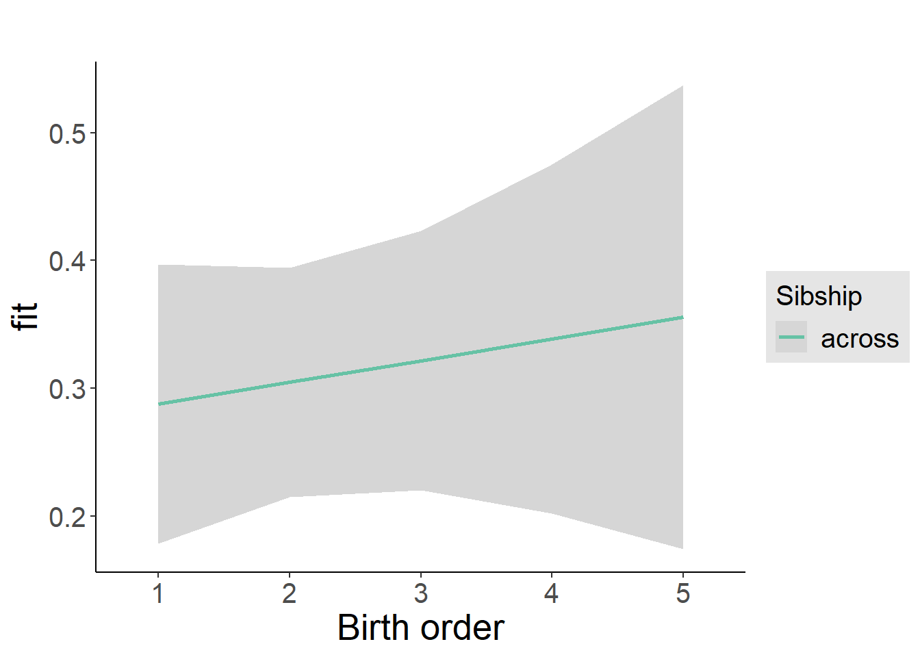
Add Birth Order Factor
Model Summary
m3_birthorder_nonlinear = update(m1_covariates_only, formula = . ~ . + birth_order_nonlinear)
tidy(m3_birthorder_nonlinear, conf.int = T, conf.level = 0.995)| effect | group | term | estimate | std.error | statistic | df | p.value | conf.low | conf.high |
|---|---|---|---|---|---|---|---|---|---|
| fixed | NA | (Intercept) | -4.244 | 5.147 | -0.8246 | 2034 | 0.4097 | -18.69 | 10.2 |
| fixed | NA | poly(age, 3, raw = TRUE)1 | 0.511 | 0.5387 | 0.9486 | 2029 | 0.3429 | -1.001 | 2.023 |
| fixed | NA | poly(age, 3, raw = TRUE)2 | -0.0178 | 0.01853 | -0.9611 | 2025 | 0.3366 | -0.06981 | 0.0342 |
| fixed | NA | poly(age, 3, raw = TRUE)3 | 0.0001955 | 0.0002094 | 0.9336 | 2021 | 0.3506 | -0.0003923 | 0.0007833 |
| fixed | NA | male | -0.1389 | 0.03975 | -3.494 | 2116 | 0.0004862 | -0.2505 | -0.0273 |
| fixed | NA | sibling_count3 | 0.01598 | 0.06678 | 0.2393 | 1740 | 0.8109 | -0.1715 | 0.2034 |
| fixed | NA | sibling_count4 | -0.04317 | 0.07014 | -0.6155 | 1715 | 0.5383 | -0.24 | 0.1537 |
| fixed | NA | sibling_count5 | -0.09032 | 0.07682 | -1.176 | 1754 | 0.2398 | -0.3059 | 0.1253 |
| fixed | NA | birth_order_nonlinear2 | 0.01225 | 0.0468 | 0.2617 | 1752 | 0.7936 | -0.1191 | 0.1436 |
| fixed | NA | birth_order_nonlinear3 | -0.005 | 0.05721 | -0.0874 | 1910 | 0.9304 | -0.1656 | 0.1556 |
| fixed | NA | birth_order_nonlinear4 | 0.05054 | 0.07616 | 0.6636 | 2066 | 0.507 | -0.1632 | 0.2643 |
| fixed | NA | birth_order_nonlinear5 | 0.1295 | 0.1094 | 1.184 | 2033 | 0.2367 | -0.1777 | 0.4367 |
| ran_pars | mother_pidlink | sd__(Intercept) | 0.5629 | NA | NA | NA | NA | NA | NA |
| ran_pars | Residual | sd__Observation | 0.8213 | NA | NA | NA | NA | NA | NA |
Coefficient Plot
plot_birthorder(m3_birthorder_nonlinear, separate = FALSE)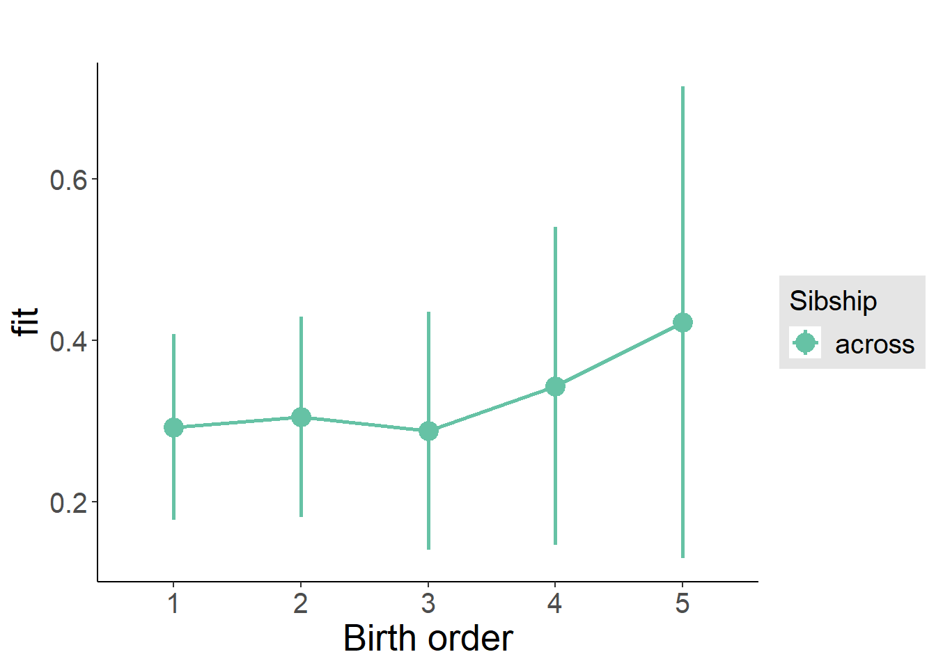
Add Interaction
Model Summary
m4_interaction = update(m3_birthorder_nonlinear, formula = . ~ . - birth_order_nonlinear - sibling_count + count_birth_order)
tidy(m4_interaction, conf.int = T, conf.level = 0.995)| effect | group | term | estimate | std.error | statistic | df | p.value | conf.low | conf.high |
|---|---|---|---|---|---|---|---|---|---|
| fixed | NA | (Intercept) | -4.548 | 5.163 | -0.8809 | 2029 | 0.3785 | -19.04 | 9.944 |
| fixed | NA | poly(age, 3, raw = TRUE)1 | 0.545 | 0.5403 | 1.009 | 2024 | 0.3132 | -0.9716 | 2.062 |
| fixed | NA | poly(age, 3, raw = TRUE)2 | -0.01892 | 0.01858 | -1.019 | 2020 | 0.3085 | -0.07107 | 0.03323 |
| fixed | NA | poly(age, 3, raw = TRUE)3 | 0.0002077 | 0.00021 | 0.9891 | 2015 | 0.3227 | -0.0003817 | 0.0007971 |
| fixed | NA | male | -0.1424 | 0.03985 | -3.572 | 2111 | 0.000362 | -0.2542 | -0.03049 |
| fixed | NA | count_birth_order2/2 | -0.08478 | 0.08974 | -0.9448 | 1728 | 0.3449 | -0.3367 | 0.1671 |
| fixed | NA | count_birth_order1/3 | -0.05764 | 0.08296 | -0.6948 | 2270 | 0.4873 | -0.2905 | 0.1752 |
| fixed | NA | count_birth_order2/3 | -0.004796 | 0.08998 | -0.0533 | 2297 | 0.9575 | -0.2574 | 0.2478 |
| fixed | NA | count_birth_order3/3 | 0.04995 | 0.09765 | 0.5115 | 2297 | 0.6091 | -0.2242 | 0.324 |
| fixed | NA | count_birth_order1/4 | -0.09664 | 0.09216 | -1.049 | 2289 | 0.2944 | -0.3553 | 0.162 |
| fixed | NA | count_birth_order2/4 | -0.02682 | 0.09293 | -0.2886 | 2298 | 0.7729 | -0.2877 | 0.234 |
| fixed | NA | count_birth_order3/4 | -0.1537 | 0.09779 | -1.571 | 2284 | 0.1162 | -0.4282 | 0.1208 |
| fixed | NA | count_birth_order4/4 | 0.0291 | 0.1077 | 0.2701 | 2286 | 0.7871 | -0.2733 | 0.3315 |
| fixed | NA | count_birth_order1/5 | -0.09154 | 0.1059 | -0.8641 | 2298 | 0.3876 | -0.3889 | 0.2058 |
| fixed | NA | count_birth_order2/5 | -0.09581 | 0.1097 | -0.8731 | 2287 | 0.3827 | -0.4038 | 0.2122 |
| fixed | NA | count_birth_order3/5 | -0.1293 | 0.1091 | -1.185 | 2262 | 0.2361 | -0.4357 | 0.177 |
| fixed | NA | count_birth_order4/5 | -0.1377 | 0.1096 | -1.256 | 2262 | 0.2092 | -0.4454 | 0.17 |
| fixed | NA | count_birth_order5/5 | 0.0006132 | 0.1136 | 0.005396 | 2274 | 0.9957 | -0.3184 | 0.3196 |
| ran_pars | mother_pidlink | sd__(Intercept) | 0.5643 | NA | NA | NA | NA | NA | NA |
| ran_pars | Residual | sd__Observation | 0.8207 | NA | NA | NA | NA | NA | NA |
Coefficient Plot
plot_birthorder(m4_interaction)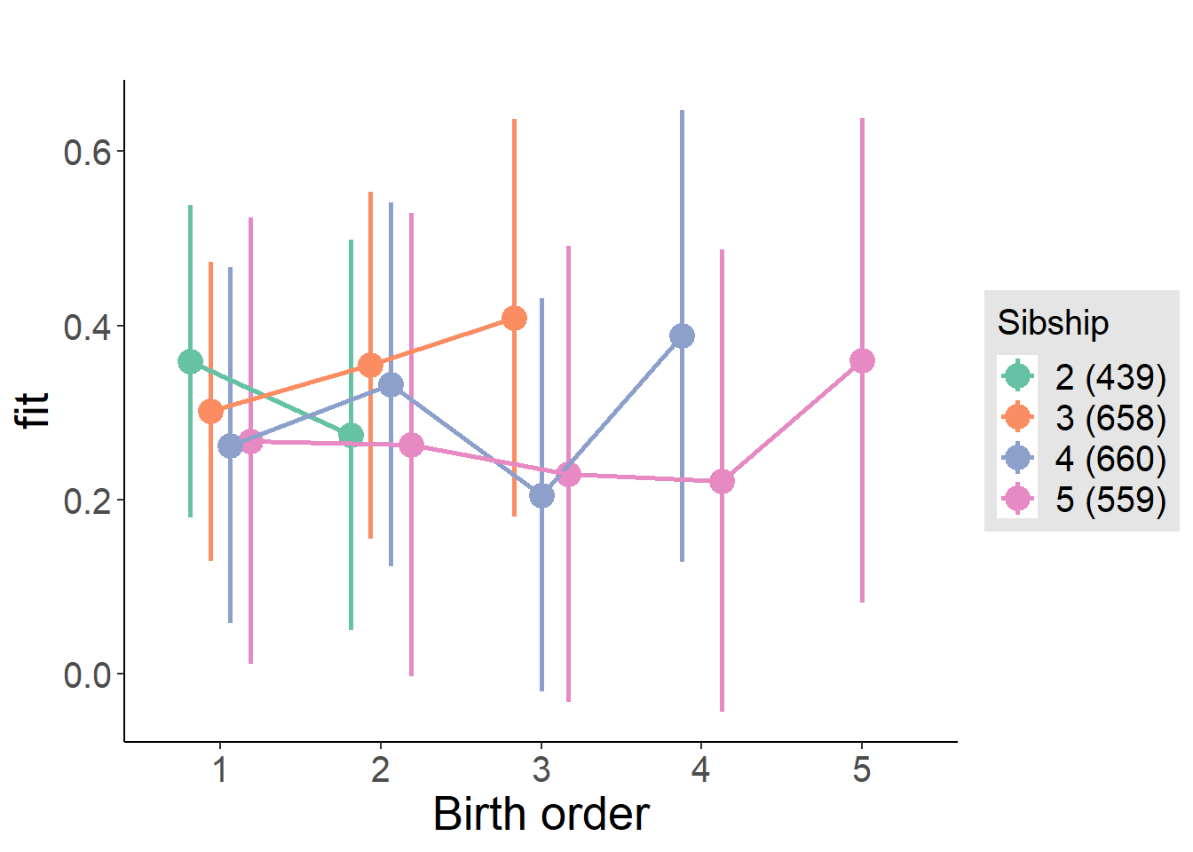
Model Comparison
###### Model 1 - Model 2
anova(m1_covariates_only, m2_birthorder_linear, m3_birthorder_nonlinear, m4_interaction)## refitting model(s) with ML (instead of REML)| Df | AIC | BIC | logLik | deviance | Chisq | Chi Df | Pr(>Chisq) |
|---|---|---|---|---|---|---|---|
| 10 | 6475 | 6532 | -3227 | 6455 | NA | NA | NA |
| 11 | 6476 | 6539 | -3227 | 6454 | 0.7542 | 1 | 0.3852 |
| 14 | 6481 | 6561 | -3226 | 6453 | 1.056 | 3 | 0.7876 |
| 20 | 6488 | 6602 | -3224 | 6448 | 5.283 | 6 | 0.508 |
Parental full sibling order
outcome_parental_m1 <- update(m2_birthorder_linear, data = birthorder %>%
mutate(sibling_count = sibling_count_genes_factor,
birth_order_nonlinear = birthorder_genes_factor,
birth_order = birthorder_genes,
count_birth_order = count_birthorder_genes
) %>%
filter(sibling_count != "1"))
compare_models_markdown(outcome_parental_m1)Basic Model
Model Summary
m1_covariates_only <- update(m2_birthorder_linear, formula = . ~ . - birth_order)
tidy(m1_covariates_only, conf.int = T, conf.level = 0.995)| effect | group | term | estimate | std.error | statistic | df | p.value | conf.low | conf.high |
|---|---|---|---|---|---|---|---|---|---|
| fixed | NA | (Intercept) | -7.26 | 4.863 | -1.493 | 2257 | 0.1356 | -20.91 | 6.392 |
| fixed | NA | poly(age, 3, raw = TRUE)1 | 0.8473 | 0.5081 | 1.668 | 2254 | 0.09555 | -0.579 | 2.274 |
| fixed | NA | poly(age, 3, raw = TRUE)2 | -0.03 | 0.01744 | -1.72 | 2250 | 0.08562 | -0.07896 | 0.01897 |
| fixed | NA | poly(age, 3, raw = TRUE)3 | 0.0003393 | 0.0001968 | 1.724 | 2246 | 0.08483 | -0.0002131 | 0.0008918 |
| fixed | NA | male | -0.171 | 0.03782 | -4.52 | 2366 | 0.000006482 | -0.2771 | -0.06479 |
| fixed | NA | sibling_count3 | 0.04392 | 0.05817 | 0.7551 | 1815 | 0.4503 | -0.1194 | 0.2072 |
| fixed | NA | sibling_count4 | -0.002439 | 0.06051 | -0.0403 | 1746 | 0.9679 | -0.1723 | 0.1674 |
| fixed | NA | sibling_count5 | -0.08814 | 0.06787 | -1.299 | 1652 | 0.1943 | -0.2786 | 0.1024 |
| ran_pars | mother_pidlink | sd__(Intercept) | 0.5551 | NA | NA | NA | NA | NA | NA |
| ran_pars | Residual | sd__Observation | 0.8223 | NA | NA | NA | NA | NA | NA |
Coefficient Plot
plot(allEffects(m1_covariates_only, confidence.level = 0.995))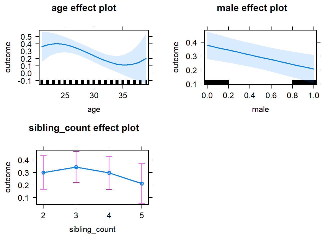
Add Birth Order Linear
Model Summary
tidy(m2_birthorder_linear, conf.int = T, conf.level = 0.995)| effect | group | term | estimate | std.error | statistic | df | p.value | conf.low | conf.high |
|---|---|---|---|---|---|---|---|---|---|
| fixed | NA | (Intercept) | -7.419 | 4.866 | -1.525 | 2257 | 0.1275 | -21.08 | 6.239 |
| fixed | NA | birth_order | 0.02083 | 0.01946 | 1.07 | 2443 | 0.2845 | -0.03379 | 0.07546 |
| fixed | NA | poly(age, 3, raw = TRUE)1 | 0.861 | 0.5083 | 1.694 | 2253 | 0.09045 | -0.5659 | 2.288 |
| fixed | NA | poly(age, 3, raw = TRUE)2 | -0.03049 | 0.01745 | -1.747 | 2249 | 0.0807 | -0.07948 | 0.01849 |
| fixed | NA | poly(age, 3, raw = TRUE)3 | 0.0003456 | 0.0001969 | 1.755 | 2246 | 0.07939 | -0.0002071 | 0.0008983 |
| fixed | NA | male | -0.1714 | 0.03782 | -4.531 | 2366 | 0.000006159 | -0.2775 | -0.06521 |
| fixed | NA | sibling_count3 | 0.03496 | 0.05876 | 0.5949 | 1832 | 0.552 | -0.13 | 0.1999 |
| fixed | NA | sibling_count4 | -0.02503 | 0.06408 | -0.3906 | 1820 | 0.6961 | -0.2049 | 0.1548 |
| fixed | NA | sibling_count5 | -0.1237 | 0.07558 | -1.637 | 1847 | 0.1017 | -0.3359 | 0.08841 |
| ran_pars | mother_pidlink | sd__(Intercept) | 0.5545 | NA | NA | NA | NA | NA | NA |
| ran_pars | Residual | sd__Observation | 0.8226 | NA | NA | NA | NA | NA | NA |
Coefficient Plot
plot_birthorder2(m2_birthorder_linear, separate = FALSE)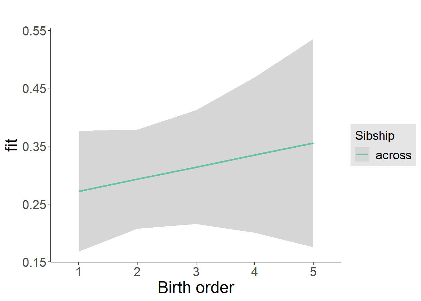
Add Birth Order Factor
Model Summary
m3_birthorder_nonlinear = update(m1_covariates_only, formula = . ~ . + birth_order_nonlinear)
tidy(m3_birthorder_nonlinear, conf.int = T, conf.level = 0.995)| effect | group | term | estimate | std.error | statistic | df | p.value | conf.low | conf.high |
|---|---|---|---|---|---|---|---|---|---|
| fixed | NA | (Intercept) | -7.26 | 4.869 | -1.491 | 2253 | 0.1361 | -20.93 | 6.406 |
| fixed | NA | poly(age, 3, raw = TRUE)1 | 0.8481 | 0.5087 | 1.667 | 2249 | 0.09563 | -0.5799 | 2.276 |
| fixed | NA | poly(age, 3, raw = TRUE)2 | -0.03006 | 0.01746 | -1.721 | 2245 | 0.08531 | -0.07908 | 0.01896 |
| fixed | NA | poly(age, 3, raw = TRUE)3 | 0.000341 | 0.0001971 | 1.73 | 2242 | 0.08372 | -0.0002122 | 0.0008941 |
| fixed | NA | male | -0.1718 | 0.03785 | -4.538 | 2365 | 0.000005949 | -0.278 | -0.06553 |
| fixed | NA | sibling_count3 | 0.04227 | 0.05942 | 0.7113 | 1885 | 0.477 | -0.1245 | 0.2091 |
| fixed | NA | sibling_count4 | -0.02761 | 0.06492 | -0.4253 | 1871 | 0.6707 | -0.2098 | 0.1546 |
| fixed | NA | sibling_count5 | -0.1347 | 0.07655 | -1.76 | 1892 | 0.07856 | -0.3496 | 0.08015 |
| fixed | NA | birth_order_nonlinear2 | -0.01548 | 0.04403 | -0.3515 | 1881 | 0.7252 | -0.1391 | 0.1081 |
| fixed | NA | birth_order_nonlinear3 | -0.002459 | 0.05451 | -0.04511 | 2068 | 0.964 | -0.1555 | 0.1505 |
| fixed | NA | birth_order_nonlinear4 | 0.1047 | 0.07371 | 1.42 | 2305 | 0.1557 | -0.1022 | 0.3116 |
| fixed | NA | birth_order_nonlinear5 | 0.106 | 0.1168 | 0.9069 | 2177 | 0.3646 | -0.222 | 0.4339 |
| ran_pars | mother_pidlink | sd__(Intercept) | 0.5549 | NA | NA | NA | NA | NA | NA |
| ran_pars | Residual | sd__Observation | 0.8226 | NA | NA | NA | NA | NA | NA |
Coefficient Plot
plot_birthorder(m3_birthorder_nonlinear, separate = FALSE)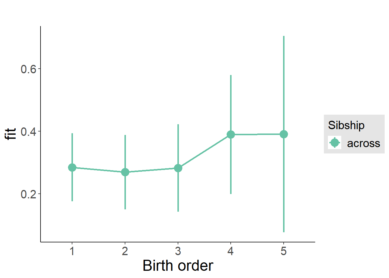
Add Interaction
Model Summary
m4_interaction = update(m3_birthorder_nonlinear, formula = . ~ . - birth_order_nonlinear - sibling_count + count_birth_order)
tidy(m4_interaction, conf.int = T, conf.level = 0.995)| effect | group | term | estimate | std.error | statistic | df | p.value | conf.low | conf.high |
|---|---|---|---|---|---|---|---|---|---|
| fixed | NA | (Intercept) | -7.118 | 4.874 | -1.46 | 2248 | 0.1443 | -20.8 | 6.564 |
| fixed | NA | poly(age, 3, raw = TRUE)1 | 0.8378 | 0.5093 | 1.645 | 2244 | 0.1001 | -0.5917 | 2.267 |
| fixed | NA | poly(age, 3, raw = TRUE)2 | -0.02978 | 0.01748 | -1.703 | 2241 | 0.08867 | -0.07885 | 0.0193 |
| fixed | NA | poly(age, 3, raw = TRUE)3 | 0.0003385 | 0.0001973 | 1.716 | 2237 | 0.08633 | -0.0002153 | 0.0008922 |
| fixed | NA | male | -0.1732 | 0.03795 | -4.564 | 2361 | 0.000005264 | -0.2797 | -0.06669 |
| fixed | NA | count_birth_order2/2 | -0.08601 | 0.07696 | -1.118 | 1909 | 0.2639 | -0.302 | 0.13 |
| fixed | NA | count_birth_order1/3 | -0.003876 | 0.0734 | -0.0528 | 2501 | 0.9579 | -0.2099 | 0.2021 |
| fixed | NA | count_birth_order2/3 | 0.03461 | 0.08104 | 0.4271 | 2535 | 0.6694 | -0.1929 | 0.2621 |
| fixed | NA | count_birth_order3/3 | 0.01203 | 0.08771 | 0.1371 | 2531 | 0.8909 | -0.2342 | 0.2582 |
| fixed | NA | count_birth_order1/4 | -0.05514 | 0.08648 | -0.6376 | 2530 | 0.5238 | -0.2979 | 0.1876 |
| fixed | NA | count_birth_order2/4 | -0.02637 | 0.08806 | -0.2995 | 2531 | 0.7646 | -0.2735 | 0.2208 |
| fixed | NA | count_birth_order3/4 | -0.1175 | 0.08939 | -1.314 | 2522 | 0.1889 | -0.3684 | 0.1334 |
| fixed | NA | count_birth_order4/4 | 0.07005 | 0.09583 | 0.731 | 2530 | 0.4649 | -0.199 | 0.3391 |
| fixed | NA | count_birth_order1/5 | -0.1812 | 0.1112 | -1.629 | 2531 | 0.1033 | -0.4935 | 0.131 |
| fixed | NA | count_birth_order2/5 | -0.2549 | 0.1175 | -2.17 | 2495 | 0.03012 | -0.5847 | 0.07487 |
| fixed | NA | count_birth_order3/5 | -0.05634 | 0.1067 | -0.5283 | 2499 | 0.5974 | -0.3557 | 0.243 |
| fixed | NA | count_birth_order4/5 | -0.08139 | 0.1075 | -0.7574 | 2503 | 0.4489 | -0.383 | 0.2202 |
| fixed | NA | count_birth_order5/5 | -0.05191 | 0.1161 | -0.447 | 2493 | 0.6549 | -0.3779 | 0.2741 |
| ran_pars | mother_pidlink | sd__(Intercept) | 0.5565 | NA | NA | NA | NA | NA | NA |
| ran_pars | Residual | sd__Observation | 0.822 | NA | NA | NA | NA | NA | NA |
Coefficient Plot
plot_birthorder(m4_interaction)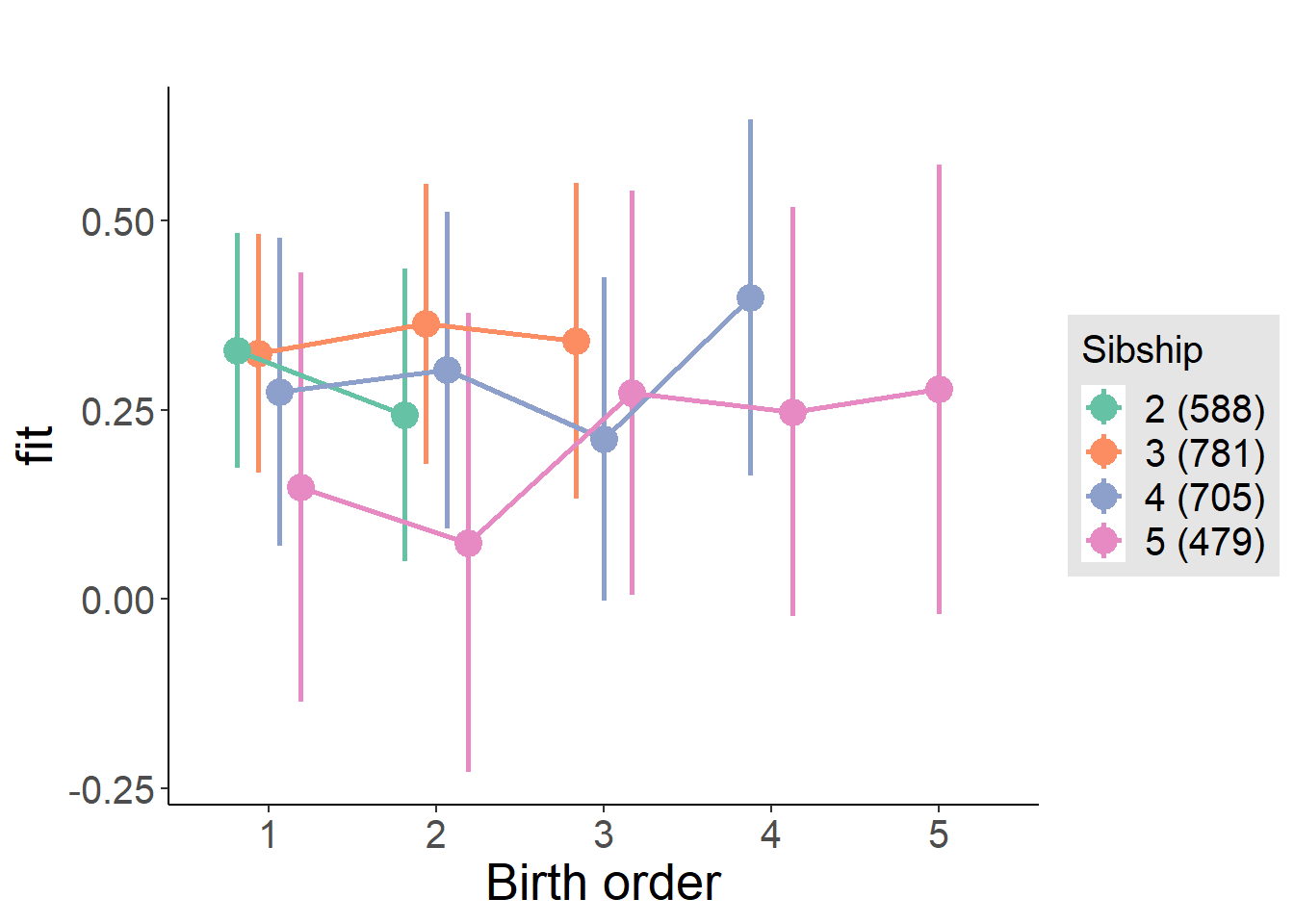
Model Comparison
###### Model 1 - Model 2
anova(m1_covariates_only, m2_birthorder_linear, m3_birthorder_nonlinear, m4_interaction)## refitting model(s) with ML (instead of REML)| Df | AIC | BIC | logLik | deviance | Chisq | Chi Df | Pr(>Chisq) |
|---|---|---|---|---|---|---|---|
| 10 | 7120 | 7179 | -3550 | 7100 | NA | NA | NA |
| 11 | 7121 | 7185 | -3550 | 7099 | 1.15 | 1 | 0.2835 |
| 14 | 7125 | 7207 | -3548 | 7097 | 2.16 | 3 | 0.5399 |
| 20 | 7132 | 7249 | -3546 | 7092 | 4.957 | 6 | 0.5494 |
Compare birth order specifications
library(coefplot)
multiplot(outcome_naive_m1, outcome_preg_m1, outcome_uterus_m1, outcome_parental_m1, dodgeHeight = 0.6,
intercept = FALSE)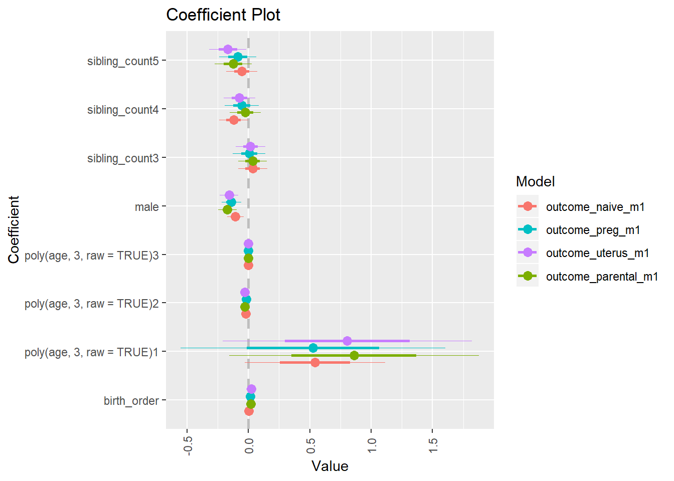
Raven 2007 young
birthorder <- birthorder %>% mutate(outcome = raven_2007_young)
model = lmer(outcome ~ birth_order + poly(age, 3, raw = TRUE) + male + sibling_count + (1 | mother_pidlink),
data = birthorder)
compare_birthorder_specs(model)Naive birth order
outcome_naive_m1 <- update(m2_birthorder_linear, data = birthorder %>%
mutate(sibling_count = sibling_count_naive_factor,
birth_order_nonlinear = birthorder_naive_factor,
birth_order = birthorder_naive,
count_birth_order = count_birthorder_naive) %>%
filter(sibling_count != "1"))
compare_models_markdown(outcome_naive_m1)Basic Model
Model Summary
m1_covariates_only <- update(m2_birthorder_linear, formula = . ~ . - birth_order)
tidy(m1_covariates_only, conf.int = T, conf.level = 0.995)| effect | group | term | estimate | std.error | statistic | df | p.value | conf.low | conf.high |
|---|---|---|---|---|---|---|---|---|---|
| fixed | NA | (Intercept) | -6.433 | 0.5236 | -12.29 | 4641 | 3.614e-34 | -7.903 | -4.964 |
| fixed | NA | poly(age, 3, raw = TRUE)1 | 0.694 | 0.06965 | 9.964 | 4767 | 3.686e-23 | 0.4985 | 0.8895 |
| fixed | NA | poly(age, 3, raw = TRUE)2 | -0.02187 | 0.002986 | -7.324 | 4905 | 2.791e-13 | -0.03025 | -0.01349 |
| fixed | NA | poly(age, 3, raw = TRUE)3 | 0.0002023 | 0.00004179 | 4.84 | 4962 | 0.000001339 | 0.00008496 | 0.0003196 |
| fixed | NA | male | 0.05122 | 0.02458 | 2.083 | 4575 | 0.03727 | -0.01779 | 0.1202 |
| fixed | NA | sibling_count3 | -0.02576 | 0.03857 | -0.6679 | 3484 | 0.5042 | -0.134 | 0.0825 |
| fixed | NA | sibling_count4 | -0.1318 | 0.03942 | -3.343 | 3281 | 0.0008389 | -0.2424 | -0.02112 |
| fixed | NA | sibling_count5 | -0.1461 | 0.04256 | -3.432 | 3053 | 0.0006071 | -0.2655 | -0.0266 |
| ran_pars | mother_pidlink | sd__(Intercept) | 0.4987 | NA | NA | NA | NA | NA | NA |
| ran_pars | Residual | sd__Observation | 0.7462 | NA | NA | NA | NA | NA | NA |
Coefficient Plot
plot(allEffects(m1_covariates_only, confidence.level = 0.995))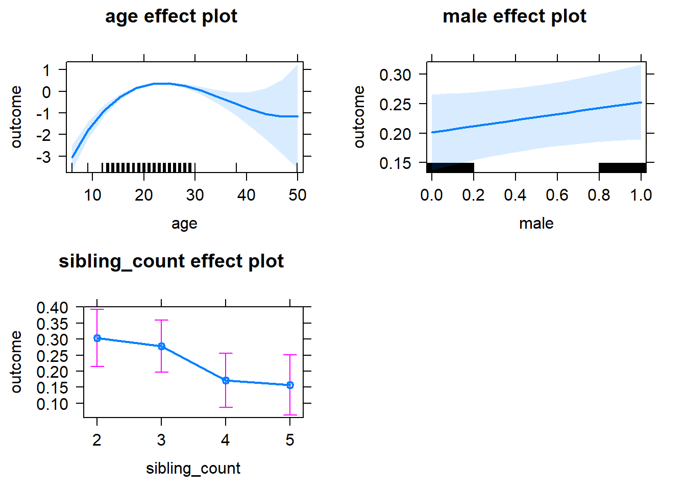
Add Birth Order Linear
Model Summary
tidy(m2_birthorder_linear, conf.int = T, conf.level = 0.995)| effect | group | term | estimate | std.error | statistic | df | p.value | conf.low | conf.high |
|---|---|---|---|---|---|---|---|---|---|
| fixed | NA | (Intercept) | -6.505 | 0.5243 | -12.41 | 4639 | 8.419e-35 | -7.977 | -5.034 |
| fixed | NA | birth_order | 0.02885 | 0.01212 | 2.379 | 4571 | 0.01738 | -0.005183 | 0.06288 |
| fixed | NA | poly(age, 3, raw = TRUE)1 | 0.697 | 0.06964 | 10.01 | 4764 | 2.366e-23 | 0.5015 | 0.8924 |
| fixed | NA | poly(age, 3, raw = TRUE)2 | -0.02194 | 0.002984 | -7.35 | 4903 | 2.311e-13 | -0.03031 | -0.01356 |
| fixed | NA | poly(age, 3, raw = TRUE)3 | 0.0002029 | 0.00004177 | 4.856 | 4961 | 0.000001235 | 0.00008559 | 0.0003201 |
| fixed | NA | male | 0.05018 | 0.02458 | 2.042 | 4577 | 0.04125 | -0.01882 | 0.1192 |
| fixed | NA | sibling_count3 | -0.03891 | 0.03893 | -0.9996 | 3518 | 0.3176 | -0.1482 | 0.07036 |
| fixed | NA | sibling_count4 | -0.1614 | 0.04131 | -3.907 | 3450 | 0.00009519 | -0.2773 | -0.04544 |
| fixed | NA | sibling_count5 | -0.1963 | 0.04747 | -4.136 | 3402 | 0.00003623 | -0.3295 | -0.06307 |
| ran_pars | mother_pidlink | sd__(Intercept) | 0.4973 | NA | NA | NA | NA | NA | NA |
| ran_pars | Residual | sd__Observation | 0.7465 | NA | NA | NA | NA | NA | NA |
Coefficient Plot
plot_birthorder2(m2_birthorder_linear, separate = FALSE)
Add Birth Order Factor
Model Summary
m3_birthorder_nonlinear = update(m1_covariates_only, formula = . ~ . + birth_order_nonlinear)
tidy(m3_birthorder_nonlinear, conf.int = T, conf.level = 0.995)| effect | group | term | estimate | std.error | statistic | df | p.value | conf.low | conf.high |
|---|---|---|---|---|---|---|---|---|---|
| fixed | NA | (Intercept) | -6.542 | 0.5234 | -12.5 | 4646 | 2.81e-35 | -8.011 | -5.073 |
| fixed | NA | poly(age, 3, raw = TRUE)1 | 0.7033 | 0.06956 | 10.11 | 4764 | 8.509e-24 | 0.5081 | 0.8986 |
| fixed | NA | poly(age, 3, raw = TRUE)2 | -0.02219 | 0.002981 | -7.445 | 4901 | 1.138e-13 | -0.03056 | -0.01383 |
| fixed | NA | poly(age, 3, raw = TRUE)3 | 0.0002061 | 0.00004172 | 4.939 | 4958 | 0.0000008103 | 0.00008896 | 0.0003232 |
| fixed | NA | male | 0.05027 | 0.02454 | 2.048 | 4572 | 0.04058 | -0.01862 | 0.1192 |
| fixed | NA | sibling_count3 | -0.02031 | 0.03928 | -0.517 | 3616 | 0.6052 | -0.1306 | 0.08996 |
| fixed | NA | sibling_count4 | -0.1473 | 0.04174 | -3.528 | 3565 | 0.0004234 | -0.2644 | -0.03011 |
| fixed | NA | sibling_count5 | -0.193 | 0.04777 | -4.041 | 3429 | 0.0000543 | -0.3271 | -0.05896 |
| fixed | NA | birth_order_nonlinear2 | 0.08362 | 0.02887 | 2.897 | 3533 | 0.003792 | 0.002595 | 0.1646 |
| fixed | NA | birth_order_nonlinear3 | -0.02977 | 0.03561 | -0.8362 | 3807 | 0.4031 | -0.1297 | 0.07017 |
| fixed | NA | birth_order_nonlinear4 | 0.1277 | 0.04753 | 2.686 | 4128 | 0.00725 | -0.005731 | 0.2611 |
| fixed | NA | birth_order_nonlinear5 | 0.1784 | 0.06796 | 2.625 | 4355 | 0.008702 | -0.01239 | 0.3691 |
| ran_pars | mother_pidlink | sd__(Intercept) | 0.4969 | NA | NA | NA | NA | NA | NA |
| ran_pars | Residual | sd__Observation | 0.7452 | NA | NA | NA | NA | NA | NA |
Coefficient Plot
plot_birthorder(m3_birthorder_nonlinear, separate = FALSE)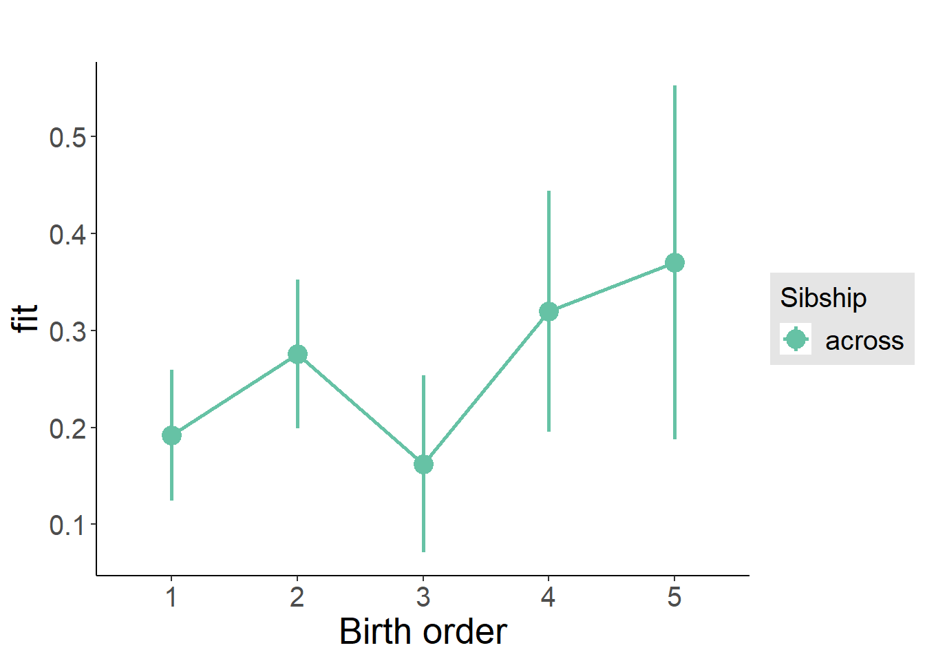
Add Interaction
Model Summary
m4_interaction = update(m3_birthorder_nonlinear, formula = . ~ . - birth_order_nonlinear - sibling_count + count_birth_order)
tidy(m4_interaction, conf.int = T, conf.level = 0.995)| effect | group | term | estimate | std.error | statistic | df | p.value | conf.low | conf.high |
|---|---|---|---|---|---|---|---|---|---|
| fixed | NA | (Intercept) | -6.531 | 0.524 | -12.46 | 4640 | 4.283e-35 | -8.002 | -5.06 |
| fixed | NA | poly(age, 3, raw = TRUE)1 | 0.7027 | 0.0696 | 10.1 | 4757 | 9.917e-24 | 0.5073 | 0.898 |
| fixed | NA | poly(age, 3, raw = TRUE)2 | -0.02216 | 0.002983 | -7.43 | 4894 | 1.277e-13 | -0.03053 | -0.01379 |
| fixed | NA | poly(age, 3, raw = TRUE)3 | 0.0002055 | 0.00004175 | 4.924 | 4952 | 0.0000008769 | 0.00008836 | 0.0003227 |
| fixed | NA | male | 0.04974 | 0.02457 | 2.025 | 4569 | 0.04297 | -0.01923 | 0.1187 |
| fixed | NA | count_birth_order2/2 | 0.0618 | 0.05382 | 1.148 | 3631 | 0.2509 | -0.08927 | 0.2129 |
| fixed | NA | count_birth_order1/3 | -0.03876 | 0.04778 | -0.8111 | 4867 | 0.4173 | -0.1729 | 0.09537 |
| fixed | NA | count_birth_order2/3 | 0.07324 | 0.05267 | 1.391 | 4952 | 0.1644 | -0.07459 | 0.2211 |
| fixed | NA | count_birth_order3/3 | -0.05428 | 0.05912 | -0.9181 | 4943 | 0.3586 | -0.2202 | 0.1117 |
| fixed | NA | count_birth_order1/4 | -0.1691 | 0.05447 | -3.105 | 4942 | 0.001911 | -0.322 | -0.01625 |
| fixed | NA | count_birth_order2/4 | -0.08263 | 0.05566 | -1.484 | 4952 | 0.1377 | -0.2389 | 0.07362 |
| fixed | NA | count_birth_order3/4 | -0.1807 | 0.05818 | -3.105 | 4923 | 0.001911 | -0.344 | -0.01736 |
| fixed | NA | count_birth_order4/4 | 0.01402 | 0.0635 | 0.2208 | 4903 | 0.8252 | -0.1642 | 0.1923 |
| fixed | NA | count_birth_order1/5 | -0.1613 | 0.06624 | -2.436 | 4944 | 0.0149 | -0.3473 | 0.0246 |
| fixed | NA | count_birth_order2/5 | -0.1047 | 0.06989 | -1.498 | 4859 | 0.1342 | -0.3009 | 0.09148 |
| fixed | NA | count_birth_order3/5 | -0.2337 | 0.06655 | -3.512 | 4853 | 0.0004491 | -0.4205 | -0.0469 |
| fixed | NA | count_birth_order4/5 | -0.1226 | 0.06986 | -1.755 | 4828 | 0.07933 | -0.3187 | 0.07349 |
| fixed | NA | count_birth_order5/5 | -0.02349 | 0.06791 | -0.3459 | 4919 | 0.7294 | -0.2141 | 0.1671 |
| ran_pars | mother_pidlink | sd__(Intercept) | 0.4965 | NA | NA | NA | NA | NA | NA |
| ran_pars | Residual | sd__Observation | 0.7458 | NA | NA | NA | NA | NA | NA |
Coefficient Plot
plot_birthorder(m4_interaction)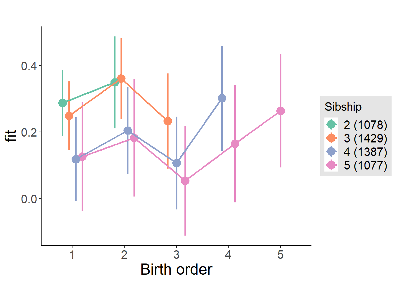
Model Comparison
###### Model 1 - Model 2
anova(m1_covariates_only, m2_birthorder_linear, m3_birthorder_nonlinear, m4_interaction)## refitting model(s) with ML (instead of REML)| Df | AIC | BIC | logLik | deviance | Chisq | Chi Df | Pr(>Chisq) |
|---|---|---|---|---|---|---|---|
| 10 | 12870 | 12935 | -6425 | 12850 | NA | NA | NA |
| 11 | 12866 | 12938 | -6422 | 12844 | 5.668 | 1 | 0.01727 |
| 14 | 12854 | 12945 | -6413 | 12826 | 17.76 | 3 | 0.0004918 |
| 20 | 12864 | 12994 | -6412 | 12824 | 2.581 | 6 | 0.8593 |
Maternal birth order
outcome_uterus_m1 <- update(m2_birthorder_linear, data = birthorder %>%
mutate(sibling_count = sibling_count_uterus_alive_factor,
birth_order_nonlinear = birthorder_uterus_alive_factor,
birth_order = birthorder_uterus_alive,
count_birth_order = count_birthorder_uterus_alive) %>%
filter(sibling_count != "1"))
compare_models_markdown(outcome_uterus_m1)Basic Model
Model Summary
m1_covariates_only <- update(m2_birthorder_linear, formula = . ~ . - birth_order)
tidy(m1_covariates_only, conf.int = T, conf.level = 0.995)| effect | group | term | estimate | std.error | statistic | df | p.value | conf.low | conf.high |
|---|---|---|---|---|---|---|---|---|---|
| fixed | NA | (Intercept) | -5.65 | 1.263 | -4.474 | 3433 | 0.000007923 | -9.195 | -2.105 |
| fixed | NA | poly(age, 3, raw = TRUE)1 | 0.5643 | 0.1931 | 2.922 | 3413 | 0.003503 | 0.02217 | 1.107 |
| fixed | NA | poly(age, 3, raw = TRUE)2 | -0.01493 | 0.009604 | -1.555 | 3398 | 0.1201 | -0.04189 | 0.01203 |
| fixed | NA | poly(age, 3, raw = TRUE)3 | 0.00008698 | 0.0001554 | 0.5597 | 3385 | 0.5757 | -0.0003492 | 0.0005232 |
| fixed | NA | male | 0.01296 | 0.0256 | 0.5061 | 4143 | 0.6128 | -0.0589 | 0.08482 |
| fixed | NA | sibling_count3 | -0.01646 | 0.03515 | -0.4682 | 3081 | 0.6397 | -0.1151 | 0.08222 |
| fixed | NA | sibling_count4 | -0.1213 | 0.03977 | -3.051 | 2771 | 0.002303 | -0.233 | -0.009699 |
| fixed | NA | sibling_count5 | -0.1898 | 0.04805 | -3.95 | 2653 | 0.00008025 | -0.3247 | -0.05491 |
| ran_pars | mother_pidlink | sd__(Intercept) | 0.4866 | NA | NA | NA | NA | NA | NA |
| ran_pars | Residual | sd__Observation | 0.7318 | NA | NA | NA | NA | NA | NA |
Coefficient Plot
plot(allEffects(m1_covariates_only, confidence.level = 0.995))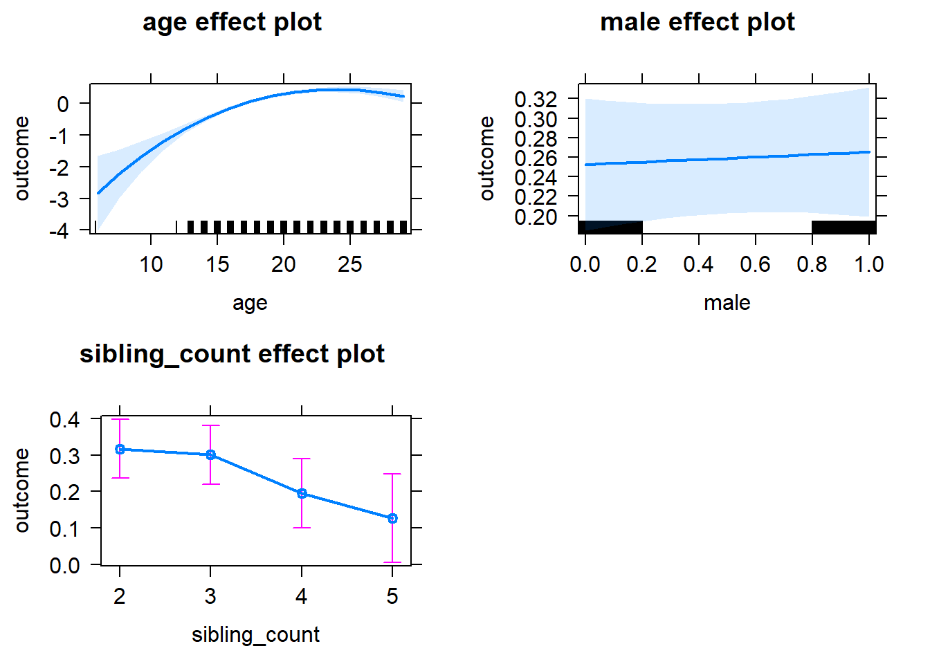
Add Birth Order Linear
Model Summary
tidy(m2_birthorder_linear, conf.int = T, conf.level = 0.995)| effect | group | term | estimate | std.error | statistic | df | p.value | conf.low | conf.high |
|---|---|---|---|---|---|---|---|---|---|
| fixed | NA | (Intercept) | -5.806 | 1.266 | -4.584 | 3439 | 0.000004713 | -9.361 | -2.251 |
| fixed | NA | birth_order | 0.02364 | 0.01404 | 1.684 | 4282 | 0.0922 | -0.01576 | 0.06304 |
| fixed | NA | poly(age, 3, raw = TRUE)1 | 0.582 | 0.1935 | 3.008 | 3413 | 0.002647 | 0.03893 | 1.125 |
| fixed | NA | poly(age, 3, raw = TRUE)2 | -0.01576 | 0.009618 | -1.638 | 3396 | 0.1014 | -0.04276 | 0.01124 |
| fixed | NA | poly(age, 3, raw = TRUE)3 | 0.0001001 | 0.0001556 | 0.6429 | 3384 | 0.5203 | -0.0003368 | 0.0005369 |
| fixed | NA | male | 0.0123 | 0.0256 | 0.4805 | 4145 | 0.6309 | -0.05956 | 0.08417 |
| fixed | NA | sibling_count3 | -0.02788 | 0.03578 | -0.7792 | 3130 | 0.4359 | -0.1283 | 0.07256 |
| fixed | NA | sibling_count4 | -0.1492 | 0.04304 | -3.466 | 2994 | 0.0005361 | -0.27 | -0.02835 |
| fixed | NA | sibling_count5 | -0.2374 | 0.05571 | -4.261 | 3083 | 0.00002091 | -0.3938 | -0.08102 |
| ran_pars | mother_pidlink | sd__(Intercept) | 0.4853 | NA | NA | NA | NA | NA | NA |
| ran_pars | Residual | sd__Observation | 0.7323 | NA | NA | NA | NA | NA | NA |
Coefficient Plot
plot_birthorder2(m2_birthorder_linear, separate = FALSE)
Add Birth Order Factor
Model Summary
m3_birthorder_nonlinear = update(m1_covariates_only, formula = . ~ . + birth_order_nonlinear)
tidy(m3_birthorder_nonlinear, conf.int = T, conf.level = 0.995)| effect | group | term | estimate | std.error | statistic | df | p.value | conf.low | conf.high |
|---|---|---|---|---|---|---|---|---|---|
| fixed | NA | (Intercept) | -5.85 | 1.266 | -4.62 | 3439 | 0.000003988 | -9.405 | -2.295 |
| fixed | NA | poly(age, 3, raw = TRUE)1 | 0.5909 | 0.1936 | 3.052 | 3413 | 0.002288 | 0.04749 | 1.134 |
| fixed | NA | poly(age, 3, raw = TRUE)2 | -0.01618 | 0.009624 | -1.682 | 3397 | 0.09274 | -0.0432 | 0.01083 |
| fixed | NA | poly(age, 3, raw = TRUE)3 | 0.0001066 | 0.0001557 | 0.6847 | 3385 | 0.4936 | -0.0003305 | 0.0005437 |
| fixed | NA | male | 0.01195 | 0.02561 | 0.4667 | 4141 | 0.6407 | -0.05994 | 0.08384 |
| fixed | NA | sibling_count3 | -0.0216 | 0.03637 | -0.5939 | 3252 | 0.5526 | -0.1237 | 0.08049 |
| fixed | NA | sibling_count4 | -0.141 | 0.0438 | -3.219 | 3092 | 0.001301 | -0.2639 | -0.01803 |
| fixed | NA | sibling_count5 | -0.2377 | 0.05743 | -4.138 | 3154 | 0.00003592 | -0.3989 | -0.07645 |
| fixed | NA | birth_order_nonlinear2 | 0.04965 | 0.02924 | 1.698 | 2986 | 0.08955 | -0.03241 | 0.1317 |
| fixed | NA | birth_order_nonlinear3 | 0.02137 | 0.03923 | 0.5447 | 3590 | 0.586 | -0.08875 | 0.1315 |
| fixed | NA | birth_order_nonlinear4 | 0.0674 | 0.05402 | 1.248 | 4007 | 0.2122 | -0.08424 | 0.2191 |
| fixed | NA | birth_order_nonlinear5 | 0.1342 | 0.0845 | 1.588 | 3990 | 0.1123 | -0.103 | 0.3714 |
| ran_pars | mother_pidlink | sd__(Intercept) | 0.4856 | NA | NA | NA | NA | NA | NA |
| ran_pars | Residual | sd__Observation | 0.7322 | NA | NA | NA | NA | NA | NA |
Coefficient Plot
plot_birthorder(m3_birthorder_nonlinear, separate = FALSE)
Add Interaction
Model Summary
m4_interaction = update(m3_birthorder_nonlinear, formula = . ~ . - birth_order_nonlinear - sibling_count + count_birth_order)
tidy(m4_interaction, conf.int = T, conf.level = 0.995)| effect | group | term | estimate | std.error | statistic | df | p.value | conf.low | conf.high |
|---|---|---|---|---|---|---|---|---|---|
| fixed | NA | (Intercept) | -5.846 | 1.267 | -4.614 | 3436 | 0.000004091 | -9.402 | -2.289 |
| fixed | NA | poly(age, 3, raw = TRUE)1 | 0.591 | 0.1937 | 3.052 | 3411 | 0.002294 | 0.04736 | 1.135 |
| fixed | NA | poly(age, 3, raw = TRUE)2 | -0.01619 | 0.009628 | -1.682 | 3394 | 0.09269 | -0.04322 | 0.01083 |
| fixed | NA | poly(age, 3, raw = TRUE)3 | 0.0001071 | 0.0001558 | 0.6872 | 3382 | 0.492 | -0.0003302 | 0.0005443 |
| fixed | NA | male | 0.01191 | 0.02564 | 0.4647 | 4135 | 0.6422 | -0.06005 | 0.08388 |
| fixed | NA | count_birth_order2/2 | 0.02876 | 0.04692 | 0.6131 | 3275 | 0.5398 | -0.1029 | 0.1605 |
| fixed | NA | count_birth_order1/3 | -0.05858 | 0.04469 | -1.311 | 4375 | 0.19 | -0.184 | 0.06687 |
| fixed | NA | count_birth_order2/3 | 0.05075 | 0.04865 | 1.043 | 4420 | 0.2969 | -0.08581 | 0.1873 |
| fixed | NA | count_birth_order3/3 | 0.01289 | 0.05426 | 0.2375 | 4420 | 0.8122 | -0.1394 | 0.1652 |
| fixed | NA | count_birth_order1/4 | -0.1245 | 0.0602 | -2.069 | 4422 | 0.03862 | -0.2935 | 0.04444 |
| fixed | NA | count_birth_order2/4 | -0.1546 | 0.06015 | -2.571 | 4384 | 0.01018 | -0.3235 | 0.01421 |
| fixed | NA | count_birth_order3/4 | -0.1275 | 0.06275 | -2.031 | 4296 | 0.04229 | -0.3036 | 0.04868 |
| fixed | NA | count_birth_order4/4 | -0.04852 | 0.06224 | -0.7796 | 4419 | 0.4357 | -0.2232 | 0.1262 |
| fixed | NA | count_birth_order1/5 | -0.172 | 0.09099 | -1.89 | 4351 | 0.05884 | -0.4274 | 0.08346 |
| fixed | NA | count_birth_order2/5 | -0.1145 | 0.0961 | -1.192 | 4111 | 0.2335 | -0.3843 | 0.1553 |
| fixed | NA | count_birth_order3/5 | -0.2707 | 0.08464 | -3.198 | 4209 | 0.001394 | -0.5082 | -0.03309 |
| fixed | NA | count_birth_order4/5 | -0.2367 | 0.07949 | -2.978 | 4303 | 0.002919 | -0.4598 | -0.01358 |
| fixed | NA | count_birth_order5/5 | -0.1166 | 0.0769 | -1.516 | 4408 | 0.1295 | -0.3325 | 0.09926 |
| ran_pars | mother_pidlink | sd__(Intercept) | 0.4864 | NA | NA | NA | NA | NA | NA |
| ran_pars | Residual | sd__Observation | 0.7317 | NA | NA | NA | NA | NA | NA |
Coefficient Plot
plot_birthorder(m4_interaction)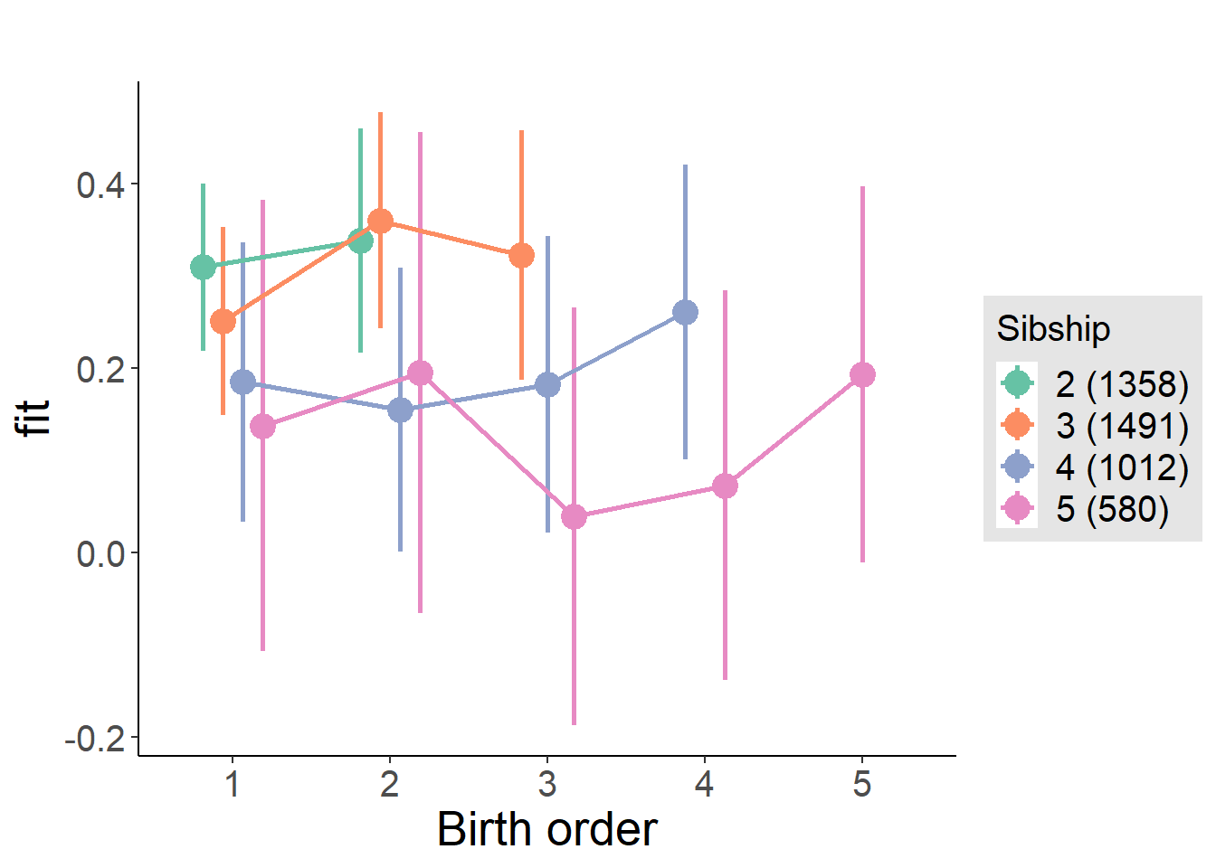
Model Comparison
###### Model 1 - Model 2
anova(m1_covariates_only, m2_birthorder_linear, m3_birthorder_nonlinear, m4_interaction)## refitting model(s) with ML (instead of REML)| Df | AIC | BIC | logLik | deviance | Chisq | Chi Df | Pr(>Chisq) |
|---|---|---|---|---|---|---|---|
| 10 | 11327 | 11391 | -5653 | 11307 | NA | NA | NA |
| 11 | 11326 | 11397 | -5652 | 11304 | 2.841 | 1 | 0.0919 |
| 14 | 11330 | 11420 | -5651 | 11302 | 2.208 | 3 | 0.5303 |
| 20 | 11335 | 11463 | -5648 | 11295 | 6.6 | 6 | 0.3595 |
Maternal pregnancy order
outcome_preg_m1 <- update(m2_birthorder_linear, data = birthorder %>%
mutate(sibling_count = sibling_count_uterus_preg_factor,
birth_order_nonlinear = birthorder_uterus_preg_factor,
birth_order = birthorder_uterus_preg,
count_birth_order = count_birthorder_uterus_preg
) %>%
filter(sibling_count != "1"))
compare_models_markdown(outcome_preg_m1)Basic Model
Model Summary
m1_covariates_only <- update(m2_birthorder_linear, formula = . ~ . - birth_order)
tidy(m1_covariates_only, conf.int = T, conf.level = 0.995)| effect | group | term | estimate | std.error | statistic | df | p.value | conf.low | conf.high |
|---|---|---|---|---|---|---|---|---|---|
| fixed | NA | (Intercept) | -5.436 | 1.292 | -4.209 | 3112 | 0.00002636 | -9.062 | -1.811 |
| fixed | NA | poly(age, 3, raw = TRUE)1 | 0.5392 | 0.1977 | 2.728 | 3090 | 0.006404 | -0.01558 | 1.094 |
| fixed | NA | poly(age, 3, raw = TRUE)2 | -0.01401 | 0.009838 | -1.424 | 3075 | 0.1546 | -0.04162 | 0.01361 |
| fixed | NA | poly(age, 3, raw = TRUE)3 | 0.00007685 | 0.0001594 | 0.4823 | 3061 | 0.6297 | -0.0003705 | 0.0005242 |
| fixed | NA | male | 0.01933 | 0.02634 | 0.734 | 3820 | 0.463 | -0.0546 | 0.09326 |
| fixed | NA | sibling_count3 | -0.03298 | 0.03778 | -0.8727 | 2926 | 0.3829 | -0.139 | 0.07309 |
| fixed | NA | sibling_count4 | -0.08832 | 0.04117 | -2.145 | 2682 | 0.03203 | -0.2039 | 0.02725 |
| fixed | NA | sibling_count5 | -0.1704 | 0.04656 | -3.66 | 2620 | 0.0002569 | -0.3011 | -0.03973 |
| ran_pars | mother_pidlink | sd__(Intercept) | 0.4984 | NA | NA | NA | NA | NA | NA |
| ran_pars | Residual | sd__Observation | 0.7204 | NA | NA | NA | NA | NA | NA |
Coefficient Plot
plot(allEffects(m1_covariates_only, confidence.level = 0.995))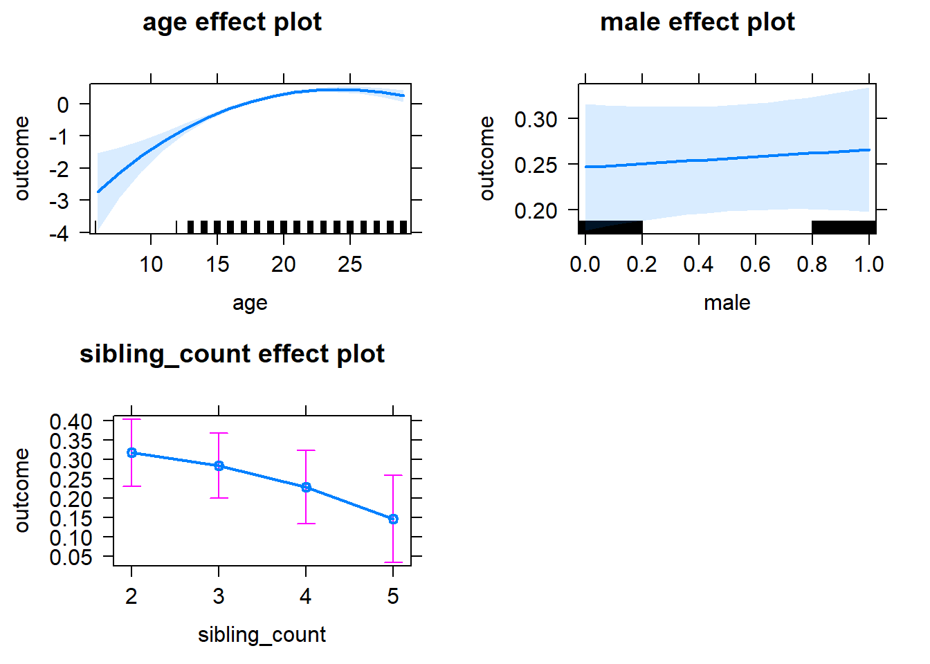
Add Birth Order Linear
Model Summary
tidy(m2_birthorder_linear, conf.int = T, conf.level = 0.995)| effect | group | term | estimate | std.error | statistic | df | p.value | conf.low | conf.high |
|---|---|---|---|---|---|---|---|---|---|
| fixed | NA | (Intercept) | -5.57 | 1.295 | -4.302 | 3117 | 0.00001746 | -9.205 | -1.935 |
| fixed | NA | birth_order | 0.02101 | 0.01395 | 1.506 | 4030 | 0.1321 | -0.01814 | 0.06015 |
| fixed | NA | poly(age, 3, raw = TRUE)1 | 0.5543 | 0.1979 | 2.8 | 3090 | 0.005137 | -0.001326 | 1.11 |
| fixed | NA | poly(age, 3, raw = TRUE)2 | -0.01472 | 0.009851 | -1.494 | 3073 | 0.1352 | -0.04237 | 0.01293 |
| fixed | NA | poly(age, 3, raw = TRUE)3 | 0.00008831 | 0.0001596 | 0.5534 | 3060 | 0.58 | -0.0003596 | 0.0005362 |
| fixed | NA | male | 0.01874 | 0.02634 | 0.7115 | 3822 | 0.4768 | -0.0552 | 0.09268 |
| fixed | NA | sibling_count3 | -0.04337 | 0.03839 | -1.13 | 2958 | 0.2587 | -0.1511 | 0.0644 |
| fixed | NA | sibling_count4 | -0.1117 | 0.04397 | -2.54 | 2857 | 0.01113 | -0.2351 | 0.01173 |
| fixed | NA | sibling_count5 | -0.2096 | 0.05329 | -3.932 | 2935 | 0.00008604 | -0.3591 | -0.05997 |
| ran_pars | mother_pidlink | sd__(Intercept) | 0.4971 | NA | NA | NA | NA | NA | NA |
| ran_pars | Residual | sd__Observation | 0.721 | NA | NA | NA | NA | NA | NA |
Coefficient Plot
plot_birthorder2(m2_birthorder_linear, separate = FALSE)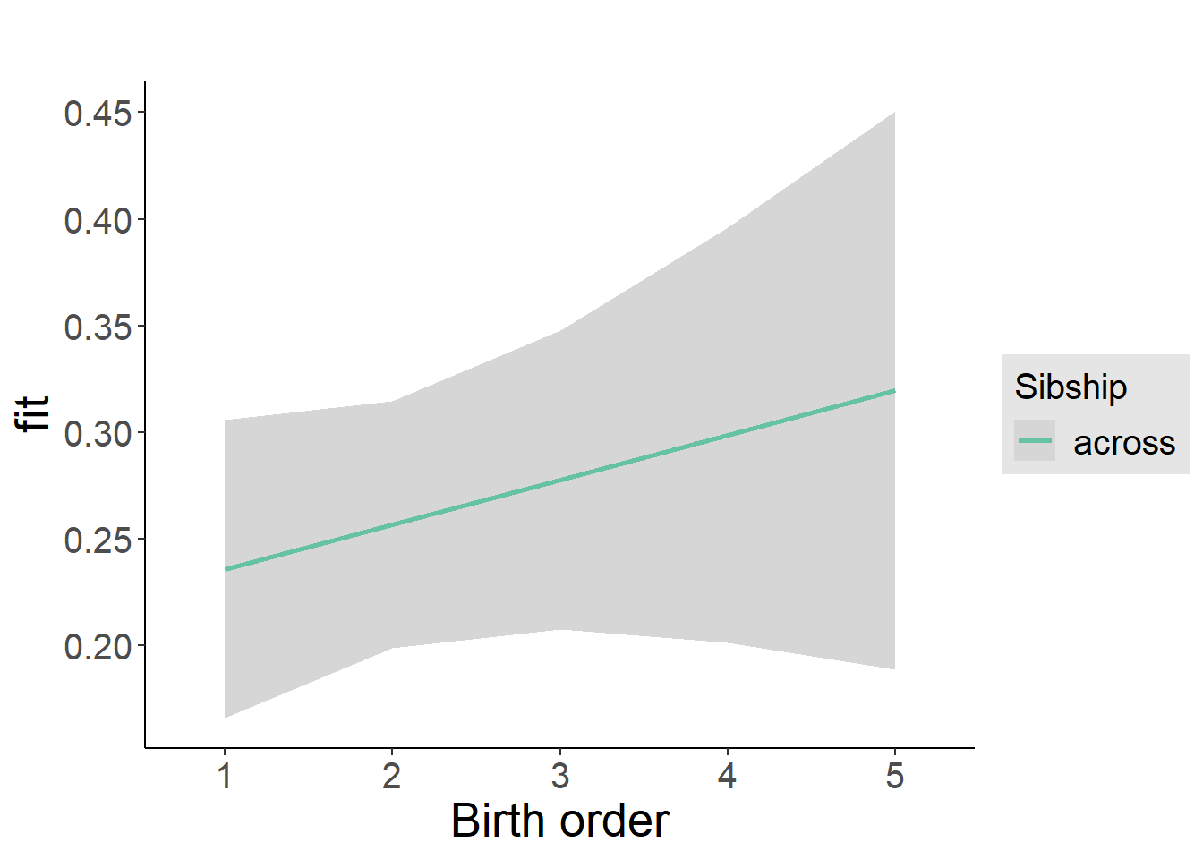
Add Birth Order Factor
Model Summary
m3_birthorder_nonlinear = update(m1_covariates_only, formula = . ~ . + birth_order_nonlinear)
tidy(m3_birthorder_nonlinear, conf.int = T, conf.level = 0.995)| effect | group | term | estimate | std.error | statistic | df | p.value | conf.low | conf.high |
|---|---|---|---|---|---|---|---|---|---|
| fixed | NA | (Intercept) | -5.649 | 1.293 | -4.368 | 3110 | 0.00001295 | -9.28 | -2.019 |
| fixed | NA | poly(age, 3, raw = TRUE)1 | 0.5672 | 0.1978 | 2.867 | 3084 | 0.004175 | 0.01181 | 1.123 |
| fixed | NA | poly(age, 3, raw = TRUE)2 | -0.01536 | 0.009847 | -1.56 | 3066 | 0.1189 | -0.043 | 0.01228 |
| fixed | NA | poly(age, 3, raw = TRUE)3 | 0.00009846 | 0.0001595 | 0.6173 | 3054 | 0.5371 | -0.0003492 | 0.0005462 |
| fixed | NA | male | 0.01948 | 0.02632 | 0.7401 | 3813 | 0.4593 | -0.05441 | 0.09338 |
| fixed | NA | sibling_count3 | -0.03149 | 0.03895 | -0.8084 | 3060 | 0.4189 | -0.1408 | 0.07785 |
| fixed | NA | sibling_count4 | -0.09791 | 0.04465 | -2.193 | 2953 | 0.02838 | -0.2232 | 0.02741 |
| fixed | NA | sibling_count5 | -0.2075 | 0.05424 | -3.825 | 2953 | 0.0001333 | -0.3598 | -0.05523 |
| fixed | NA | birth_order_nonlinear2 | 0.07433 | 0.0302 | 2.461 | 2789 | 0.01391 | -0.01045 | 0.1591 |
| fixed | NA | birth_order_nonlinear3 | -0.01017 | 0.03971 | -0.2562 | 3361 | 0.7978 | -0.1216 | 0.1013 |
| fixed | NA | birth_order_nonlinear4 | 0.06452 | 0.05393 | 1.196 | 3667 | 0.2316 | -0.08687 | 0.2159 |
| fixed | NA | birth_order_nonlinear5 | 0.1475 | 0.08088 | 1.824 | 3852 | 0.0682 | -0.07949 | 0.3746 |
| ran_pars | mother_pidlink | sd__(Intercept) | 0.4988 | NA | NA | NA | NA | NA | NA |
| ran_pars | Residual | sd__Observation | 0.7194 | NA | NA | NA | NA | NA | NA |
Coefficient Plot
plot_birthorder(m3_birthorder_nonlinear, separate = FALSE)
Add Interaction
Model Summary
m4_interaction = update(m3_birthorder_nonlinear, formula = . ~ . - birth_order_nonlinear - sibling_count + count_birth_order)
tidy(m4_interaction, conf.int = T, conf.level = 0.995)| effect | group | term | estimate | std.error | statistic | df | p.value | conf.low | conf.high |
|---|---|---|---|---|---|---|---|---|---|
| fixed | NA | (Intercept) | -5.638 | 1.292 | -4.364 | 3097 | 0.00001321 | -9.265 | -2.011 |
| fixed | NA | poly(age, 3, raw = TRUE)1 | 0.5661 | 0.1977 | 2.863 | 3072 | 0.004218 | 0.01116 | 1.121 |
| fixed | NA | poly(age, 3, raw = TRUE)2 | -0.01537 | 0.009839 | -1.562 | 3055 | 0.1183 | -0.04299 | 0.01225 |
| fixed | NA | poly(age, 3, raw = TRUE)3 | 0.00009993 | 0.0001594 | 0.6271 | 3042 | 0.5307 | -0.0003474 | 0.0005473 |
| fixed | NA | male | 0.0172 | 0.02632 | 0.6536 | 3803 | 0.5134 | -0.05668 | 0.09108 |
| fixed | NA | count_birth_order2/2 | 0.08626 | 0.05096 | 1.693 | 2992 | 0.0906 | -0.05678 | 0.2293 |
| fixed | NA | count_birth_order1/3 | -0.06631 | 0.04797 | -1.382 | 4087 | 0.1669 | -0.201 | 0.06834 |
| fixed | NA | count_birth_order2/3 | 0.058 | 0.05152 | 1.126 | 4128 | 0.2603 | -0.08662 | 0.2026 |
| fixed | NA | count_birth_order3/3 | 0.0198 | 0.05786 | 0.3422 | 4124 | 0.7323 | -0.1426 | 0.1822 |
| fixed | NA | count_birth_order1/4 | -0.0688 | 0.06015 | -1.144 | 4129 | 0.2528 | -0.2377 | 0.1001 |
| fixed | NA | count_birth_order2/4 | -0.06173 | 0.06068 | -1.017 | 4099 | 0.3091 | -0.2321 | 0.1086 |
| fixed | NA | count_birth_order3/4 | -0.1235 | 0.06374 | -1.937 | 4014 | 0.05277 | -0.3024 | 0.05544 |
| fixed | NA | count_birth_order4/4 | 0.003209 | 0.06534 | 0.04911 | 4121 | 0.9608 | -0.1802 | 0.1866 |
| fixed | NA | count_birth_order1/5 | -0.0709 | 0.08158 | -0.869 | 4078 | 0.3849 | -0.2999 | 0.1581 |
| fixed | NA | count_birth_order2/5 | -0.1033 | 0.08253 | -1.251 | 3976 | 0.2109 | -0.3349 | 0.1284 |
| fixed | NA | count_birth_order3/5 | -0.3042 | 0.07872 | -3.864 | 3956 | 0.0001135 | -0.5251 | -0.08318 |
| fixed | NA | count_birth_order4/5 | -0.1991 | 0.07917 | -2.514 | 3927 | 0.01196 | -0.4213 | 0.02316 |
| fixed | NA | count_birth_order5/5 | -0.06404 | 0.07581 | -0.8448 | 4117 | 0.3983 | -0.2768 | 0.1488 |
| ran_pars | mother_pidlink | sd__(Intercept) | 0.5015 | NA | NA | NA | NA | NA | NA |
| ran_pars | Residual | sd__Observation | 0.7174 | NA | NA | NA | NA | NA | NA |
Coefficient Plot
plot_birthorder(m4_interaction)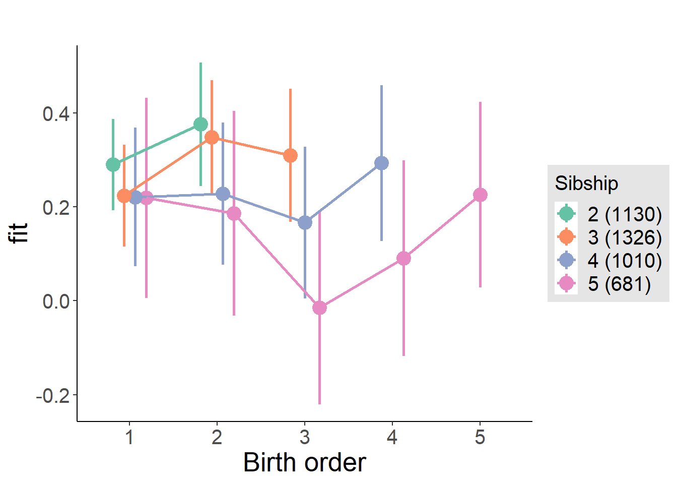
Model Comparison
###### Model 1 - Model 2
anova(m1_covariates_only, m2_birthorder_linear, m3_birthorder_nonlinear, m4_interaction)## refitting model(s) with ML (instead of REML)| Df | AIC | BIC | logLik | deviance | Chisq | Chi Df | Pr(>Chisq) |
|---|---|---|---|---|---|---|---|
| 10 | 10541 | 10604 | -5260 | 10521 | NA | NA | NA |
| 11 | 10540 | 10610 | -5259 | 10518 | 2.272 | 1 | 0.1317 |
| 14 | 10538 | 10626 | -5255 | 10510 | 8.47 | 3 | 0.03723 |
| 20 | 10539 | 10666 | -5250 | 10499 | 10.41 | 6 | 0.1084 |
Parental full sibling order
outcome_parental_m1 <- update(m2_birthorder_linear, data = birthorder %>%
mutate(sibling_count = sibling_count_genes_factor,
birth_order_nonlinear = birthorder_genes_factor,
birth_order = birthorder_genes,
count_birth_order = count_birthorder_genes
) %>%
filter(sibling_count != "1"))
compare_models_markdown(outcome_parental_m1)Basic Model
Model Summary
m1_covariates_only <- update(m2_birthorder_linear, formula = . ~ . - birth_order)
tidy(m1_covariates_only, conf.int = T, conf.level = 0.995)| effect | group | term | estimate | std.error | statistic | df | p.value | conf.low | conf.high |
|---|---|---|---|---|---|---|---|---|---|
| fixed | NA | (Intercept) | -5.019 | 1.28 | -3.92 | 3334 | 0.00009048 | -8.613 | -1.425 |
| fixed | NA | poly(age, 3, raw = TRUE)1 | 0.4672 | 0.1958 | 2.386 | 3314 | 0.01707 | -0.08233 | 1.017 |
| fixed | NA | poly(age, 3, raw = TRUE)2 | -0.01011 | 0.009731 | -1.039 | 3300 | 0.2987 | -0.03743 | 0.0172 |
| fixed | NA | poly(age, 3, raw = TRUE)3 | 0.000008366 | 0.0001574 | 0.05315 | 3288 | 0.9576 | -0.0004335 | 0.0004502 |
| fixed | NA | male | 0.009549 | 0.02598 | 0.3676 | 4048 | 0.7132 | -0.06337 | 0.08247 |
| fixed | NA | sibling_count3 | -0.009593 | 0.03549 | -0.2703 | 3018 | 0.7869 | -0.1092 | 0.09002 |
| fixed | NA | sibling_count4 | -0.1137 | 0.04033 | -2.819 | 2716 | 0.004858 | -0.2269 | -0.0004671 |
| fixed | NA | sibling_count5 | -0.1938 | 0.05042 | -3.843 | 2631 | 0.0001242 | -0.3353 | -0.05225 |
| ran_pars | mother_pidlink | sd__(Intercept) | 0.4991 | NA | NA | NA | NA | NA | NA |
| ran_pars | Residual | sd__Observation | 0.7345 | NA | NA | NA | NA | NA | NA |
Coefficient Plot
plot(allEffects(m1_covariates_only, confidence.level = 0.995))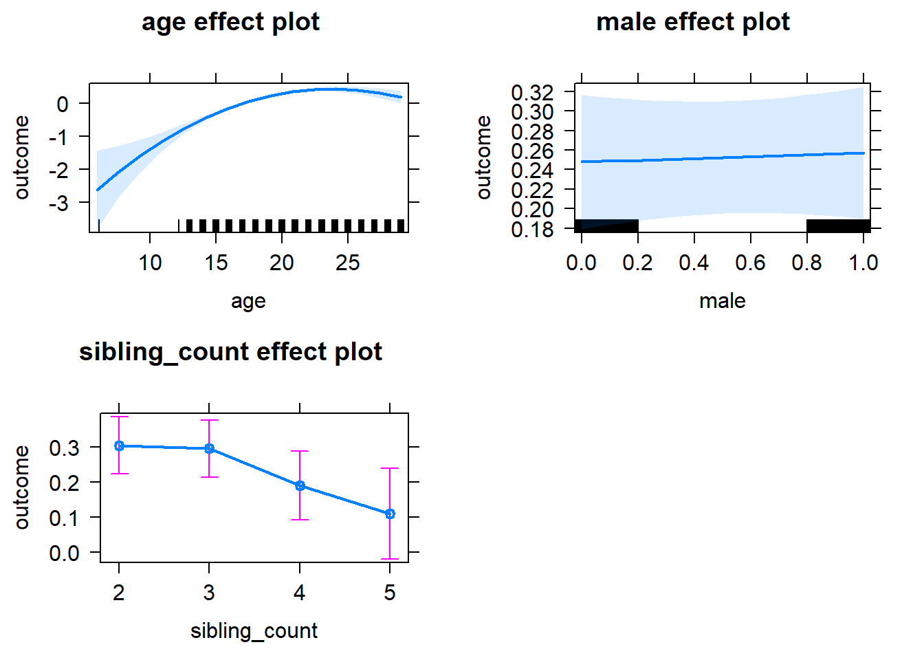
Add Birth Order Linear
Model Summary
tidy(m2_birthorder_linear, conf.int = T, conf.level = 0.995)| effect | group | term | estimate | std.error | statistic | df | p.value | conf.low | conf.high |
|---|---|---|---|---|---|---|---|---|---|
| fixed | NA | (Intercept) | -5.19 | 1.284 | -4.041 | 3340 | 0.00005431 | -8.795 | -1.585 |
| fixed | NA | birth_order | 0.02514 | 0.01436 | 1.751 | 4174 | 0.08004 | -0.01516 | 0.06544 |
| fixed | NA | poly(age, 3, raw = TRUE)1 | 0.4869 | 0.1961 | 2.483 | 3314 | 0.01307 | -0.06351 | 1.037 |
| fixed | NA | poly(age, 3, raw = TRUE)2 | -0.01105 | 0.009746 | -1.134 | 3297 | 0.257 | -0.03841 | 0.01631 |
| fixed | NA | poly(age, 3, raw = TRUE)3 | 0.0000233 | 0.0001576 | 0.1478 | 3286 | 0.8825 | -0.0004192 | 0.0004658 |
| fixed | NA | male | 0.009023 | 0.02598 | 0.3474 | 4049 | 0.7283 | -0.06389 | 0.08194 |
| fixed | NA | sibling_count3 | -0.02143 | 0.03611 | -0.5934 | 3065 | 0.553 | -0.1228 | 0.07994 |
| fixed | NA | sibling_count4 | -0.1435 | 0.04375 | -3.279 | 2945 | 0.001053 | -0.2663 | -0.02065 |
| fixed | NA | sibling_count5 | -0.2432 | 0.05775 | -4.211 | 3025 | 0.00002617 | -0.4053 | -0.08108 |
| ran_pars | mother_pidlink | sd__(Intercept) | 0.4982 | NA | NA | NA | NA | NA | NA |
| ran_pars | Residual | sd__Observation | 0.7348 | NA | NA | NA | NA | NA | NA |
Coefficient Plot
plot_birthorder2(m2_birthorder_linear, separate = FALSE)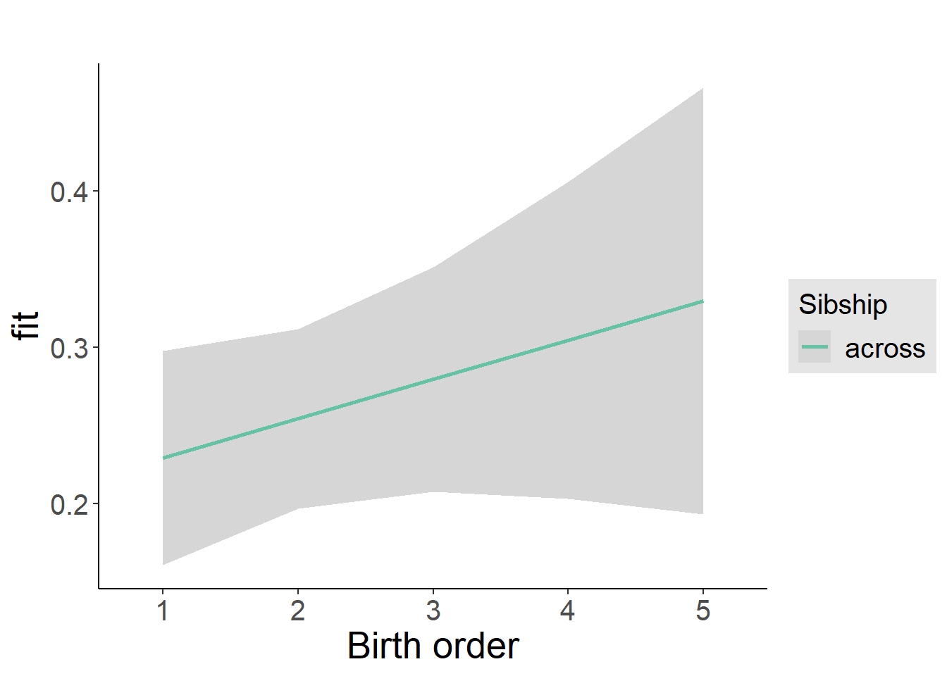
Add Birth Order Factor
Model Summary
m3_birthorder_nonlinear = update(m1_covariates_only, formula = . ~ . + birth_order_nonlinear)
tidy(m3_birthorder_nonlinear, conf.int = T, conf.level = 0.995)| effect | group | term | estimate | std.error | statistic | df | p.value | conf.low | conf.high |
|---|---|---|---|---|---|---|---|---|---|
| fixed | NA | (Intercept) | -5.19 | 1.285 | -4.039 | 3343 | 0.00005495 | -8.797 | -1.583 |
| fixed | NA | poly(age, 3, raw = TRUE)1 | 0.4888 | 0.1963 | 2.49 | 3318 | 0.01283 | -0.0623 | 1.04 |
| fixed | NA | poly(age, 3, raw = TRUE)2 | -0.01111 | 0.009758 | -1.139 | 3301 | 0.2548 | -0.03851 | 0.01628 |
| fixed | NA | poly(age, 3, raw = TRUE)3 | 0.00002383 | 0.0001578 | 0.151 | 3290 | 0.88 | -0.0004192 | 0.0004669 |
| fixed | NA | male | 0.008719 | 0.02599 | 0.3355 | 4045 | 0.7373 | -0.06423 | 0.08167 |
| fixed | NA | sibling_count3 | -0.0222 | 0.03671 | -0.6047 | 3185 | 0.5454 | -0.1252 | 0.08085 |
| fixed | NA | sibling_count4 | -0.1393 | 0.04456 | -3.125 | 3047 | 0.001793 | -0.2644 | -0.01418 |
| fixed | NA | sibling_count5 | -0.2314 | 0.05989 | -3.863 | 3099 | 0.0001142 | -0.3995 | -0.06326 |
| fixed | NA | birth_order_nonlinear2 | 0.05207 | 0.02943 | 1.769 | 2900 | 0.07694 | -0.03054 | 0.1347 |
| fixed | NA | birth_order_nonlinear3 | 0.05619 | 0.03979 | 1.412 | 3457 | 0.158 | -0.05551 | 0.1679 |
| fixed | NA | birth_order_nonlinear4 | 0.06141 | 0.05545 | 1.107 | 3895 | 0.2682 | -0.09425 | 0.2171 |
| fixed | NA | birth_order_nonlinear5 | 0.08254 | 0.09058 | 0.9112 | 3956 | 0.3622 | -0.1717 | 0.3368 |
| ran_pars | mother_pidlink | sd__(Intercept) | 0.4982 | NA | NA | NA | NA | NA | NA |
| ran_pars | Residual | sd__Observation | 0.735 | NA | NA | NA | NA | NA | NA |
Coefficient Plot
plot_birthorder(m3_birthorder_nonlinear, separate = FALSE)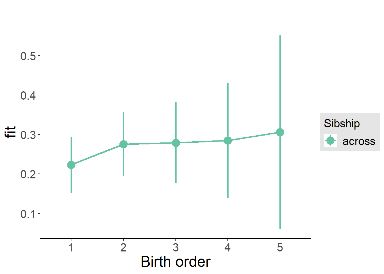
Add Interaction
Model Summary
m4_interaction = update(m3_birthorder_nonlinear, formula = . ~ . - birth_order_nonlinear - sibling_count + count_birth_order)
tidy(m4_interaction, conf.int = T, conf.level = 0.995)| effect | group | term | estimate | std.error | statistic | df | p.value | conf.low | conf.high |
|---|---|---|---|---|---|---|---|---|---|
| fixed | NA | (Intercept) | -5.182 | 1.286 | -4.03 | 3344 | 0.00005698 | -8.791 | -1.573 |
| fixed | NA | poly(age, 3, raw = TRUE)1 | 0.4879 | 0.1965 | 2.483 | 3319 | 0.01307 | -0.06363 | 1.039 |
| fixed | NA | poly(age, 3, raw = TRUE)2 | -0.01104 | 0.009765 | -1.13 | 3302 | 0.2585 | -0.03845 | 0.01638 |
| fixed | NA | poly(age, 3, raw = TRUE)3 | 0.00002227 | 0.0001579 | 0.141 | 3289 | 0.8879 | -0.0004211 | 0.0004656 |
| fixed | NA | male | 0.008893 | 0.02602 | 0.3418 | 4043 | 0.7325 | -0.06415 | 0.08194 |
| fixed | NA | count_birth_order2/2 | 0.02821 | 0.0462 | 0.6107 | 3150 | 0.5414 | -0.1015 | 0.1579 |
| fixed | NA | count_birth_order1/3 | -0.06192 | 0.04499 | -1.376 | 4311 | 0.1688 | -0.1882 | 0.06438 |
| fixed | NA | count_birth_order2/3 | 0.06353 | 0.04955 | 1.282 | 4355 | 0.1999 | -0.07557 | 0.2026 |
| fixed | NA | count_birth_order3/3 | 0.03548 | 0.0548 | 0.6474 | 4352 | 0.5174 | -0.1184 | 0.1893 |
| fixed | NA | count_birth_order1/4 | -0.1107 | 0.06157 | -1.798 | 4357 | 0.07218 | -0.2836 | 0.06211 |
| fixed | NA | count_birth_order2/4 | -0.1568 | 0.06104 | -2.569 | 4319 | 0.01024 | -0.3282 | 0.01455 |
| fixed | NA | count_birth_order3/4 | -0.1015 | 0.06339 | -1.601 | 4215 | 0.1094 | -0.2795 | 0.07642 |
| fixed | NA | count_birth_order4/4 | -0.05428 | 0.0629 | -0.8629 | 4355 | 0.3882 | -0.2308 | 0.1223 |
| fixed | NA | count_birth_order1/5 | -0.1947 | 0.0931 | -2.092 | 4298 | 0.03653 | -0.4561 | 0.06661 |
| fixed | NA | count_birth_order2/5 | -0.133 | 0.103 | -1.291 | 3995 | 0.1967 | -0.4222 | 0.1561 |
| fixed | NA | count_birth_order3/5 | -0.1812 | 0.08961 | -2.022 | 4135 | 0.04322 | -0.4328 | 0.07033 |
| fixed | NA | count_birth_order4/5 | -0.2449 | 0.08457 | -2.895 | 4209 | 0.003806 | -0.4822 | -0.007477 |
| fixed | NA | count_birth_order5/5 | -0.1625 | 0.08238 | -1.972 | 4342 | 0.04862 | -0.3937 | 0.06875 |
| ran_pars | mother_pidlink | sd__(Intercept) | 0.498 | NA | NA | NA | NA | NA | NA |
| ran_pars | Residual | sd__Observation | 0.735 | NA | NA | NA | NA | NA | NA |
Coefficient Plot
plot_birthorder(m4_interaction)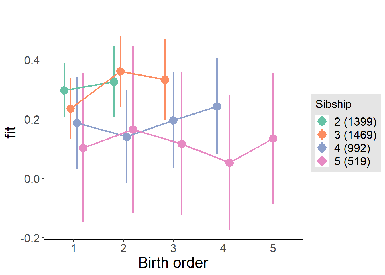
Model Comparison
###### Model 1 - Model 2
anova(m1_covariates_only, m2_birthorder_linear, m3_birthorder_nonlinear, m4_interaction)## refitting model(s) with ML (instead of REML)| Df | AIC | BIC | logLik | deviance | Chisq | Chi Df | Pr(>Chisq) |
|---|---|---|---|---|---|---|---|
| 10 | 11250 | 11314 | -5615 | 11230 | NA | NA | NA |
| 11 | 11249 | 11320 | -5614 | 11227 | 3.071 | 1 | 0.0797 |
| 14 | 11254 | 11344 | -5613 | 11226 | 1.156 | 3 | 0.7635 |
| 20 | 11260 | 11387 | -5610 | 11220 | 6.436 | 6 | 0.3761 |
Compare birth order specifications
library(coefplot)
multiplot(outcome_naive_m1, outcome_preg_m1, outcome_uterus_m1, outcome_parental_m1, dodgeHeight = 0.6,
intercept = FALSE)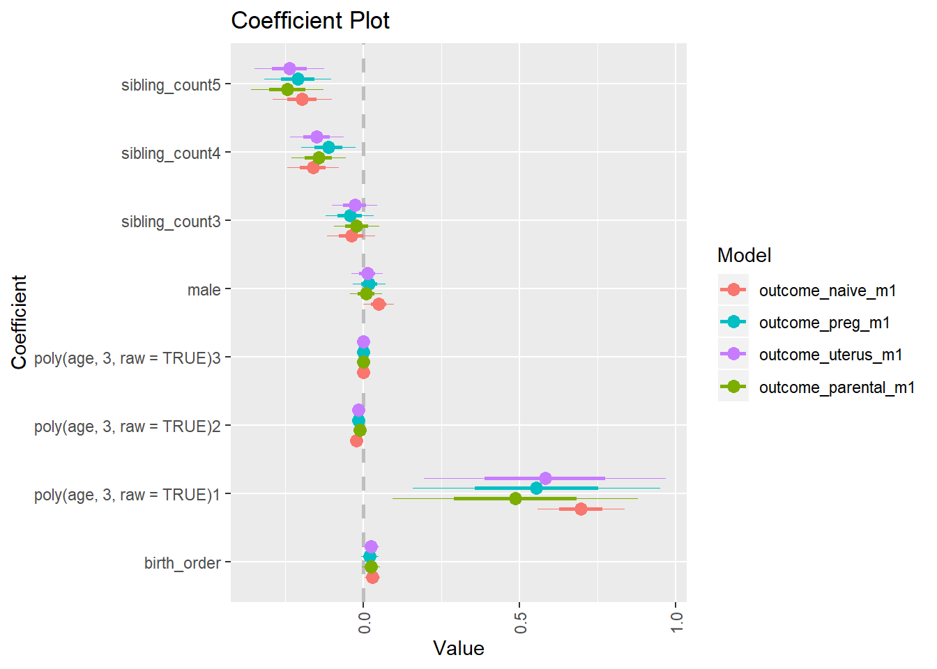
Numeracy 2007 young
birthorder <- birthorder %>% mutate(outcome = math_2007_young)
model = lmer(outcome ~ birth_order + poly(age, 3, raw = TRUE) + male + sibling_count + (1 | mother_pidlink),
data = birthorder)
compare_birthorder_specs(model)Naive birth order
outcome_naive_m1 <- update(m2_birthorder_linear, data = birthorder %>%
mutate(sibling_count = sibling_count_naive_factor,
birth_order_nonlinear = birthorder_naive_factor,
birth_order = birthorder_naive,
count_birth_order = count_birthorder_naive) %>%
filter(sibling_count != "1"))
compare_models_markdown(outcome_naive_m1)Basic Model
Model Summary
m1_covariates_only <- update(m2_birthorder_linear, formula = . ~ . - birth_order)
tidy(m1_covariates_only, conf.int = T, conf.level = 0.995)| effect | group | term | estimate | std.error | statistic | df | p.value | conf.low | conf.high |
|---|---|---|---|---|---|---|---|---|---|
| fixed | NA | (Intercept) | -6.423 | 0.5453 | -11.78 | 4640 | 1.427e-31 | -7.953 | -4.892 |
| fixed | NA | poly(age, 3, raw = TRUE)1 | 0.7323 | 0.07259 | 10.09 | 4769 | 1.075e-23 | 0.5285 | 0.936 |
| fixed | NA | poly(age, 3, raw = TRUE)2 | -0.02495 | 0.003115 | -8.009 | 4908 | 1.428e-15 | -0.03369 | -0.0162 |
| fixed | NA | poly(age, 3, raw = TRUE)3 | 0.0002604 | 0.00004366 | 5.964 | 4961 | 0.000000002627 | 0.0001379 | 0.000383 |
| fixed | NA | male | -0.1132 | 0.02559 | -4.422 | 4543 | 0.000009986 | -0.185 | -0.04134 |
| fixed | NA | sibling_count3 | 0.02256 | 0.04057 | 0.5561 | 3558 | 0.5782 | -0.09132 | 0.1364 |
| fixed | NA | sibling_count4 | -0.1283 | 0.0415 | -3.092 | 3372 | 0.002001 | -0.2448 | -0.01184 |
| fixed | NA | sibling_count5 | -0.03847 | 0.04484 | -0.858 | 3163 | 0.3909 | -0.1643 | 0.08738 |
| ran_pars | mother_pidlink | sd__(Intercept) | 0.5439 | NA | NA | NA | NA | NA | NA |
| ran_pars | Residual | sd__Observation | 0.7672 | NA | NA | NA | NA | NA | NA |
Coefficient Plot
plot(allEffects(m1_covariates_only, confidence.level = 0.995))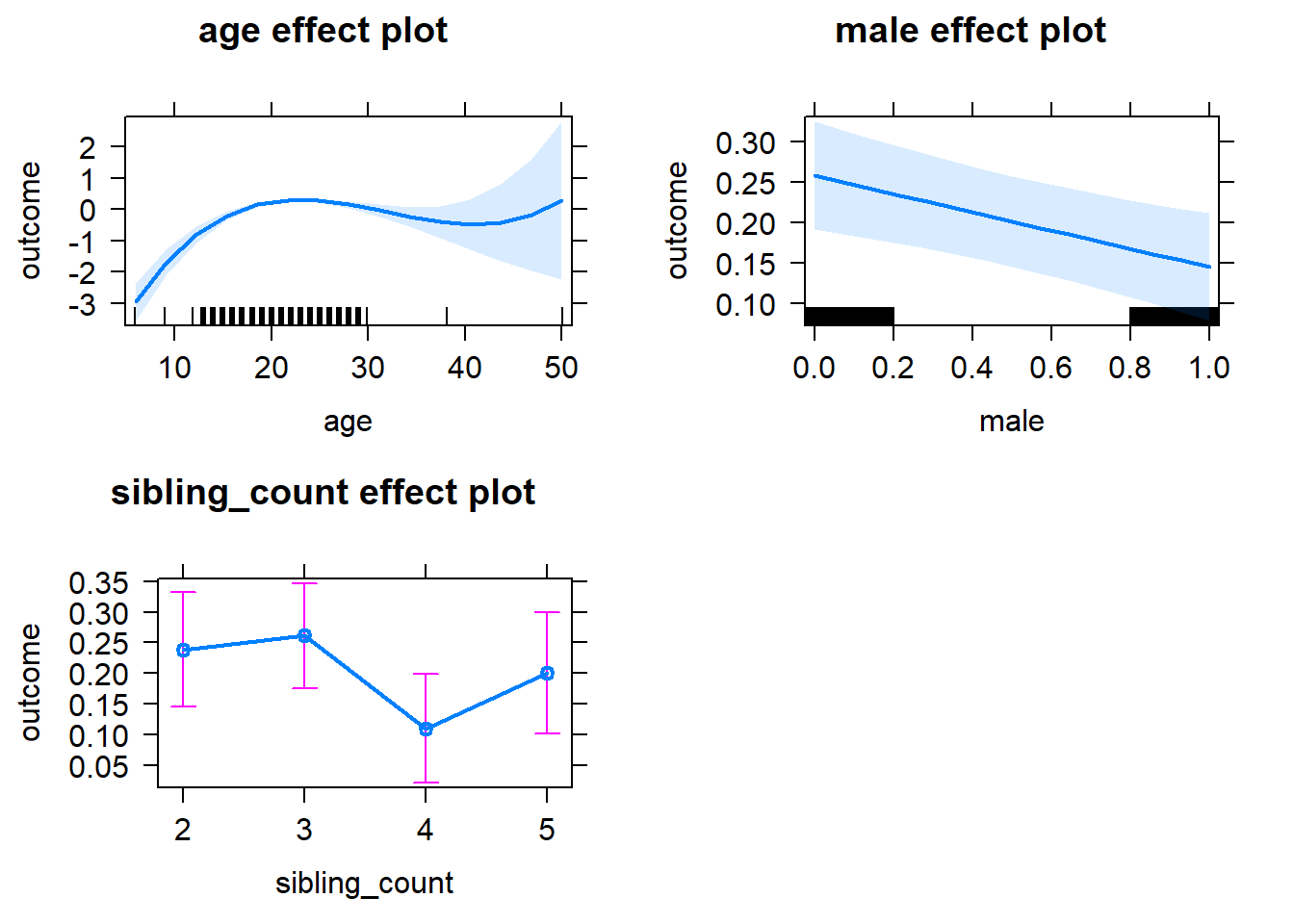
Add Birth Order Linear
Model Summary
tidy(m2_birthorder_linear, conf.int = T, conf.level = 0.995)| effect | group | term | estimate | std.error | statistic | df | p.value | conf.low | conf.high |
|---|---|---|---|---|---|---|---|---|---|
| fixed | NA | (Intercept) | -6.482 | 0.5461 | -11.87 | 4638 | 4.842e-32 | -8.015 | -4.95 |
| fixed | NA | birth_order | 0.02427 | 0.01262 | 1.923 | 4590 | 0.05455 | -0.01116 | 0.05971 |
| fixed | NA | poly(age, 3, raw = TRUE)1 | 0.7345 | 0.07258 | 10.12 | 4765 | 7.749e-24 | 0.5308 | 0.9383 |
| fixed | NA | poly(age, 3, raw = TRUE)2 | -0.02499 | 0.003114 | -8.025 | 4906 | 1.256e-15 | -0.03373 | -0.01625 |
| fixed | NA | poly(age, 3, raw = TRUE)3 | 0.0002607 | 0.00004365 | 5.973 | 4960 | 0.000000002494 | 0.0001382 | 0.0003833 |
| fixed | NA | male | -0.1141 | 0.02559 | -4.457 | 4541 | 0.000008494 | -0.1859 | -0.04223 |
| fixed | NA | sibling_count3 | 0.01144 | 0.04097 | 0.2793 | 3591 | 0.78 | -0.1036 | 0.1265 |
| fixed | NA | sibling_count4 | -0.1534 | 0.04349 | -3.527 | 3534 | 0.0004258 | -0.2754 | -0.0313 |
| fixed | NA | sibling_count5 | -0.08097 | 0.04998 | -1.62 | 3500 | 0.1053 | -0.2213 | 0.05932 |
| ran_pars | mother_pidlink | sd__(Intercept) | 0.5439 | NA | NA | NA | NA | NA | NA |
| ran_pars | Residual | sd__Observation | 0.7669 | NA | NA | NA | NA | NA | NA |
Coefficient Plot
plot_birthorder2(m2_birthorder_linear, separate = FALSE)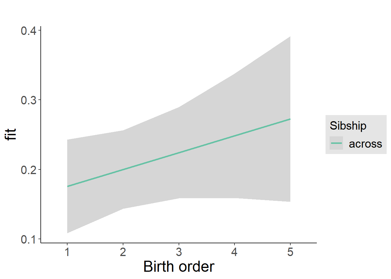
Add Birth Order Factor
Model Summary
m3_birthorder_nonlinear = update(m1_covariates_only, formula = . ~ . + birth_order_nonlinear)
tidy(m3_birthorder_nonlinear, conf.int = T, conf.level = 0.995)| effect | group | term | estimate | std.error | statistic | df | p.value | conf.low | conf.high |
|---|---|---|---|---|---|---|---|---|---|
| fixed | NA | (Intercept) | -6.496 | 0.5459 | -11.9 | 4644 | 3.519e-32 | -8.028 | -4.963 |
| fixed | NA | poly(age, 3, raw = TRUE)1 | 0.738 | 0.0726 | 10.17 | 4766 | 4.918e-24 | 0.5343 | 0.9418 |
| fixed | NA | poly(age, 3, raw = TRUE)2 | -0.02513 | 0.003115 | -8.07 | 4904 | 8.794e-16 | -0.03388 | -0.01639 |
| fixed | NA | poly(age, 3, raw = TRUE)3 | 0.0002625 | 0.00004366 | 6.014 | 4957 | 0.000000001941 | 0.00014 | 0.0003851 |
| fixed | NA | male | -0.1139 | 0.02559 | -4.452 | 4537 | 0.000008716 | -0.1857 | -0.04209 |
| fixed | NA | sibling_count3 | 0.01112 | 0.04138 | 0.2686 | 3681 | 0.7882 | -0.105 | 0.1273 |
| fixed | NA | sibling_count4 | -0.1614 | 0.04398 | -3.671 | 3639 | 0.0002451 | -0.2849 | -0.03799 |
| fixed | NA | sibling_count5 | -0.06866 | 0.05035 | -1.364 | 3525 | 0.1728 | -0.21 | 0.07267 |
| fixed | NA | birth_order_nonlinear2 | 0.06097 | 0.02998 | 2.034 | 3565 | 0.04206 | -0.02318 | 0.1451 |
| fixed | NA | birth_order_nonlinear3 | 0.04911 | 0.03702 | 1.327 | 3836 | 0.1847 | -0.0548 | 0.153 |
| fixed | NA | birth_order_nonlinear4 | 0.1212 | 0.04946 | 2.451 | 4141 | 0.0143 | -0.01763 | 0.2601 |
| fixed | NA | birth_order_nonlinear5 | 0.01766 | 0.07079 | 0.2494 | 4353 | 0.803 | -0.181 | 0.2164 |
| ran_pars | mother_pidlink | sd__(Intercept) | 0.5436 | NA | NA | NA | NA | NA | NA |
| ran_pars | Residual | sd__Observation | 0.7669 | NA | NA | NA | NA | NA | NA |
Coefficient Plot
plot_birthorder(m3_birthorder_nonlinear, separate = FALSE)
Add Interaction
Model Summary
m4_interaction = update(m3_birthorder_nonlinear, formula = . ~ . - birth_order_nonlinear - sibling_count + count_birth_order)
tidy(m4_interaction, conf.int = T, conf.level = 0.995)| effect | group | term | estimate | std.error | statistic | df | p.value | conf.low | conf.high |
|---|---|---|---|---|---|---|---|---|---|
| fixed | NA | (Intercept) | -6.501 | 0.5465 | -11.9 | 4638 | 3.67e-32 | -8.035 | -4.967 |
| fixed | NA | poly(age, 3, raw = TRUE)1 | 0.7377 | 0.07263 | 10.16 | 4759 | 5.415e-24 | 0.5338 | 0.9416 |
| fixed | NA | poly(age, 3, raw = TRUE)2 | -0.02513 | 0.003116 | -8.063 | 4897 | 9.26e-16 | -0.03387 | -0.01638 |
| fixed | NA | poly(age, 3, raw = TRUE)3 | 0.0002626 | 0.00004368 | 6.013 | 4951 | 0.000000001956 | 0.00014 | 0.0003852 |
| fixed | NA | male | -0.1135 | 0.02561 | -4.432 | 4535 | 0.000009555 | -0.1854 | -0.04162 |
| fixed | NA | count_birth_order2/2 | 0.08511 | 0.05591 | 1.522 | 3665 | 0.128 | -0.07183 | 0.2421 |
| fixed | NA | count_birth_order1/3 | 0.0339 | 0.05006 | 0.677 | 4860 | 0.4984 | -0.1066 | 0.1744 |
| fixed | NA | count_birth_order2/3 | 0.08199 | 0.0551 | 1.488 | 4951 | 0.1368 | -0.07269 | 0.2367 |
| fixed | NA | count_birth_order3/3 | 0.02926 | 0.06181 | 0.4733 | 4944 | 0.636 | -0.1443 | 0.2028 |
| fixed | NA | count_birth_order1/4 | -0.1495 | 0.05701 | -2.622 | 4940 | 0.008778 | -0.3095 | 0.01057 |
| fixed | NA | count_birth_order2/4 | -0.09275 | 0.05822 | -1.593 | 4953 | 0.1112 | -0.2562 | 0.07068 |
| fixed | NA | count_birth_order3/4 | -0.1192 | 0.06081 | -1.96 | 4924 | 0.05005 | -0.2899 | 0.05151 |
| fixed | NA | count_birth_order4/4 | -0.02441 | 0.06635 | -0.3679 | 4905 | 0.713 | -0.2107 | 0.1618 |
| fixed | NA | count_birth_order1/5 | -0.08821 | 0.06926 | -1.274 | 4944 | 0.2029 | -0.2826 | 0.1062 |
| fixed | NA | count_birth_order2/5 | -0.03633 | 0.07299 | -0.4977 | 4857 | 0.6187 | -0.2412 | 0.1686 |
| fixed | NA | count_birth_order3/5 | 0.05753 | 0.0695 | 0.8278 | 4853 | 0.4078 | -0.1376 | 0.2526 |
| fixed | NA | count_birth_order4/5 | 0.04828 | 0.07294 | 0.662 | 4826 | 0.508 | -0.1565 | 0.253 |
| fixed | NA | count_birth_order5/5 | -0.04089 | 0.07097 | -0.5761 | 4921 | 0.5646 | -0.2401 | 0.1583 |
| ran_pars | mother_pidlink | sd__(Intercept) | 0.5431 | NA | NA | NA | NA | NA | NA |
| ran_pars | Residual | sd__Observation | 0.7675 | NA | NA | NA | NA | NA | NA |
Coefficient Plot
plot_birthorder(m4_interaction)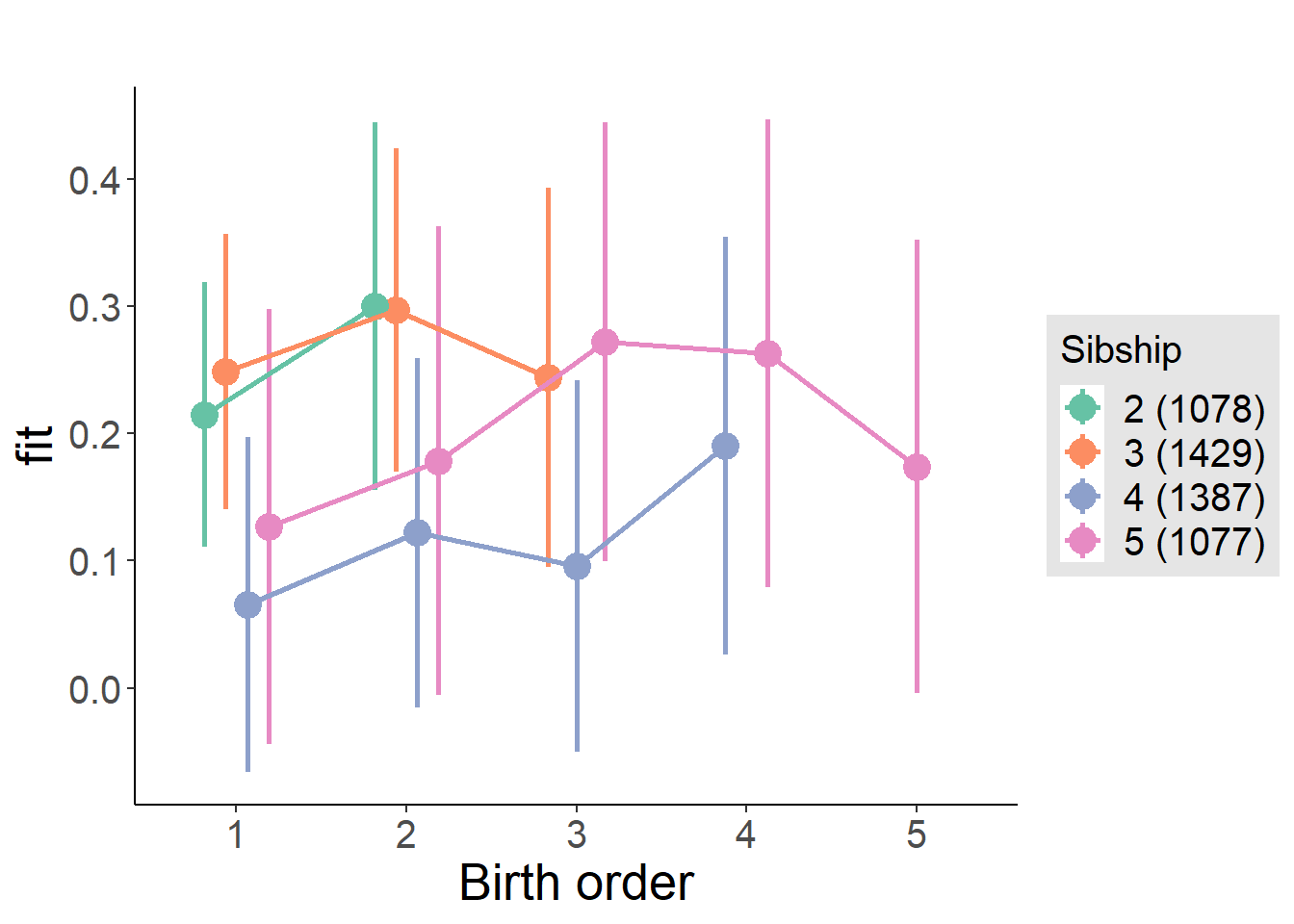
Model Comparison
###### Model 1 - Model 2
anova(m1_covariates_only, m2_birthorder_linear, m3_birthorder_nonlinear, m4_interaction)## refitting model(s) with ML (instead of REML)| Df | AIC | BIC | logLik | deviance | Chisq | Chi Df | Pr(>Chisq) |
|---|---|---|---|---|---|---|---|
| 10 | 13303 | 13368 | -6641 | 13283 | NA | NA | NA |
| 11 | 13301 | 13373 | -6640 | 13279 | 3.703 | 1 | 0.05433 |
| 14 | 13302 | 13394 | -6637 | 13274 | 4.61 | 3 | 0.2027 |
| 20 | 13311 | 13441 | -6636 | 13271 | 3.332 | 6 | 0.7661 |
Maternal birth order
outcome_uterus_m1 <- update(m2_birthorder_linear, data = birthorder %>%
mutate(sibling_count = sibling_count_uterus_alive_factor,
birth_order_nonlinear = birthorder_uterus_alive_factor,
birth_order = birthorder_uterus_alive,
count_birth_order = count_birthorder_uterus_alive) %>%
filter(sibling_count != "1"))
compare_models_markdown(outcome_uterus_m1)Basic Model
Model Summary
m1_covariates_only <- update(m2_birthorder_linear, formula = . ~ . - birth_order)
tidy(m1_covariates_only, conf.int = T, conf.level = 0.995)| effect | group | term | estimate | std.error | statistic | df | p.value | conf.low | conf.high |
|---|---|---|---|---|---|---|---|---|---|
| fixed | NA | (Intercept) | -5.27 | 1.314 | -4.011 | 3342 | 0.0000617 | -8.958 | -1.582 |
| fixed | NA | poly(age, 3, raw = TRUE)1 | 0.5413 | 0.2009 | 2.695 | 3321 | 0.007082 | -0.02258 | 1.105 |
| fixed | NA | poly(age, 3, raw = TRUE)2 | -0.01476 | 0.009989 | -1.477 | 3306 | 0.1397 | -0.0428 | 0.01328 |
| fixed | NA | poly(age, 3, raw = TRUE)3 | 0.00009009 | 0.0001616 | 0.5575 | 3293 | 0.5773 | -0.0003636 | 0.0005437 |
| fixed | NA | male | -0.1385 | 0.02677 | -5.176 | 4079 | 0.0000002376 | -0.2137 | -0.06341 |
| fixed | NA | sibling_count3 | 0.03331 | 0.03738 | 0.891 | 3159 | 0.373 | -0.07163 | 0.1382 |
| fixed | NA | sibling_count4 | -0.04248 | 0.04237 | -1.002 | 2887 | 0.3162 | -0.1614 | 0.07647 |
| fixed | NA | sibling_count5 | -0.09838 | 0.05123 | -1.92 | 2783 | 0.05491 | -0.2422 | 0.04543 |
| ran_pars | mother_pidlink | sd__(Intercept) | 0.5494 | NA | NA | NA | NA | NA | NA |
| ran_pars | Residual | sd__Observation | 0.7482 | NA | NA | NA | NA | NA | NA |
Coefficient Plot
plot(allEffects(m1_covariates_only, confidence.level = 0.995))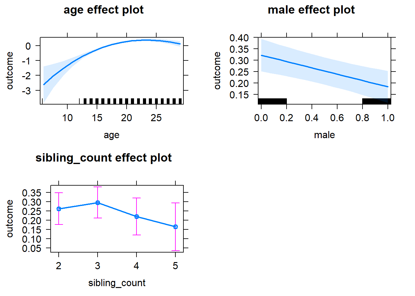
Add Birth Order Linear
Model Summary
tidy(m2_birthorder_linear, conf.int = T, conf.level = 0.995)| effect | group | term | estimate | std.error | statistic | df | p.value | conf.low | conf.high |
|---|---|---|---|---|---|---|---|---|---|
| fixed | NA | (Intercept) | -5.445 | 1.317 | -4.134 | 3347 | 0.00003651 | -9.142 | -1.748 |
| fixed | NA | birth_order | 0.02649 | 0.0147 | 1.802 | 4281 | 0.07155 | -0.01477 | 0.06775 |
| fixed | NA | poly(age, 3, raw = TRUE)1 | 0.561 | 0.2012 | 2.789 | 3319 | 0.005318 | -0.003632 | 1.126 |
| fixed | NA | poly(age, 3, raw = TRUE)2 | -0.01568 | 0.01 | -1.568 | 3302 | 0.117 | -0.04375 | 0.01239 |
| fixed | NA | poly(age, 3, raw = TRUE)3 | 0.0001047 | 0.0001618 | 0.6471 | 3290 | 0.5176 | -0.0003494 | 0.0005588 |
| fixed | NA | male | -0.1393 | 0.02676 | -5.204 | 4079 | 0.0000002042 | -0.2144 | -0.06416 |
| fixed | NA | sibling_count3 | 0.02042 | 0.03805 | 0.5367 | 3205 | 0.5915 | -0.08638 | 0.1272 |
| fixed | NA | sibling_count4 | -0.07386 | 0.0458 | -1.613 | 3103 | 0.1069 | -0.2024 | 0.0547 |
| fixed | NA | sibling_count5 | -0.1521 | 0.05925 | -2.567 | 3195 | 0.01031 | -0.3184 | 0.01423 |
| ran_pars | mother_pidlink | sd__(Intercept) | 0.5489 | NA | NA | NA | NA | NA | NA |
| ran_pars | Residual | sd__Observation | 0.7482 | NA | NA | NA | NA | NA | NA |
Coefficient Plot
plot_birthorder2(m2_birthorder_linear, separate = FALSE)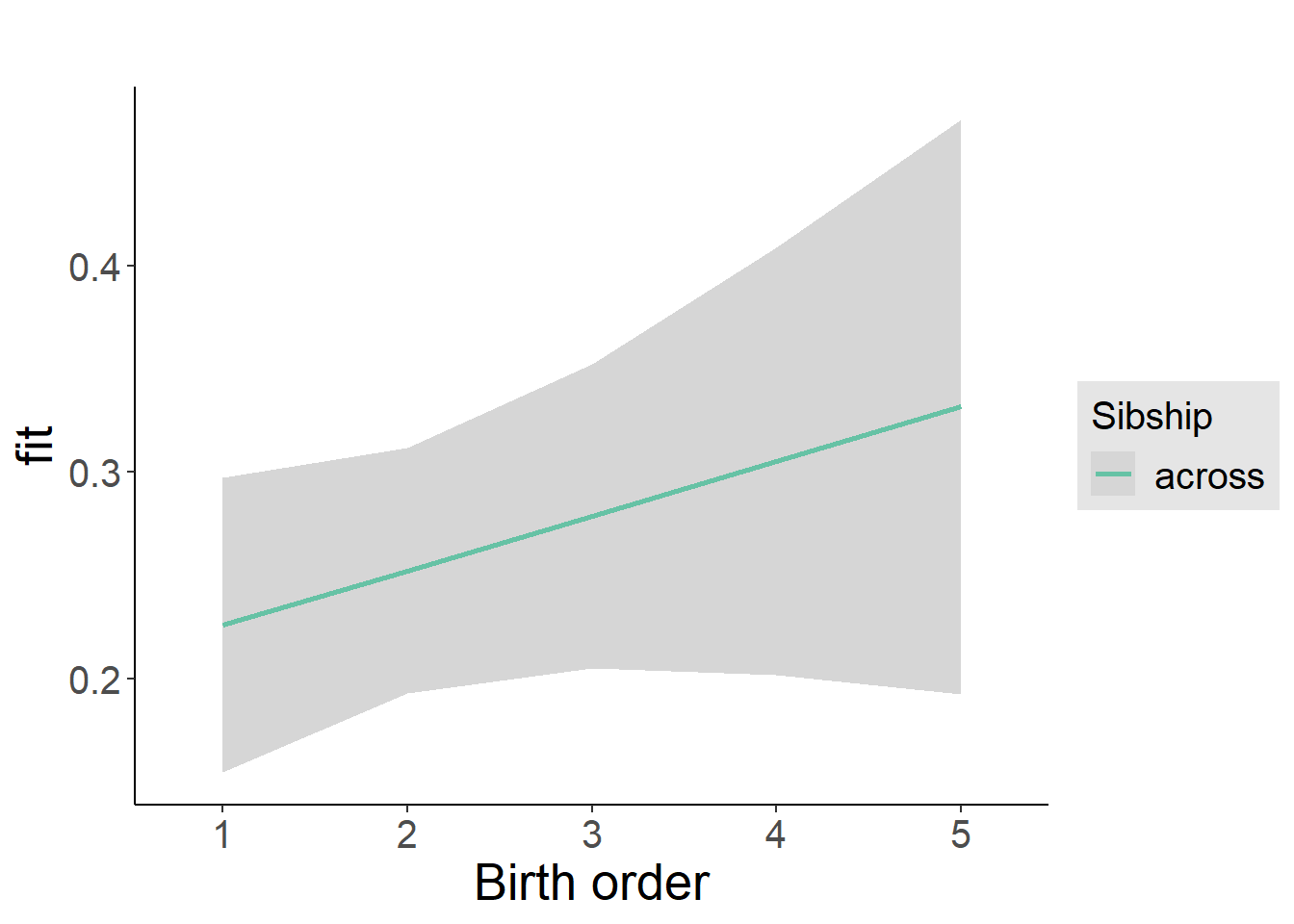
Add Birth Order Factor
Model Summary
m3_birthorder_nonlinear = update(m1_covariates_only, formula = . ~ . + birth_order_nonlinear)
tidy(m3_birthorder_nonlinear, conf.int = T, conf.level = 0.995)| effect | group | term | estimate | std.error | statistic | df | p.value | conf.low | conf.high |
|---|---|---|---|---|---|---|---|---|---|
| fixed | NA | (Intercept) | -5.451 | 1.318 | -4.136 | 3352 | 0.00003619 | -9.15 | -1.751 |
| fixed | NA | poly(age, 3, raw = TRUE)1 | 0.567 | 0.2014 | 2.815 | 3326 | 0.004901 | 0.001682 | 1.132 |
| fixed | NA | poly(age, 3, raw = TRUE)2 | -0.016 | 0.01001 | -1.598 | 3309 | 0.1101 | -0.04411 | 0.0121 |
| fixed | NA | poly(age, 3, raw = TRUE)3 | 0.0001103 | 0.000162 | 0.6807 | 3297 | 0.4961 | -0.0003444 | 0.000565 |
| fixed | NA | male | -0.1391 | 0.02678 | -5.194 | 4079 | 0.0000002154 | -0.2143 | -0.06394 |
| fixed | NA | sibling_count3 | 0.02657 | 0.03863 | 0.688 | 3320 | 0.4915 | -0.08185 | 0.135 |
| fixed | NA | sibling_count4 | -0.06915 | 0.04657 | -1.485 | 3196 | 0.1376 | -0.1999 | 0.06156 |
| fixed | NA | sibling_count5 | -0.1674 | 0.06102 | -2.744 | 3274 | 0.006111 | -0.3387 | 0.003875 |
| fixed | NA | birth_order_nonlinear2 | 0.01502 | 0.03035 | 0.495 | 3005 | 0.6206 | -0.07017 | 0.1002 |
| fixed | NA | birth_order_nonlinear3 | 0.02673 | 0.04087 | 0.654 | 3595 | 0.5132 | -0.088 | 0.1415 |
| fixed | NA | birth_order_nonlinear4 | 0.08087 | 0.05644 | 1.433 | 3990 | 0.152 | -0.07758 | 0.2393 |
| fixed | NA | birth_order_nonlinear5 | 0.1731 | 0.08827 | 1.962 | 3956 | 0.04988 | -0.07462 | 0.4209 |
| ran_pars | mother_pidlink | sd__(Intercept) | 0.5476 | NA | NA | NA | NA | NA | NA |
| ran_pars | Residual | sd__Observation | 0.7491 | NA | NA | NA | NA | NA | NA |
Coefficient Plot
plot_birthorder(m3_birthorder_nonlinear, separate = FALSE)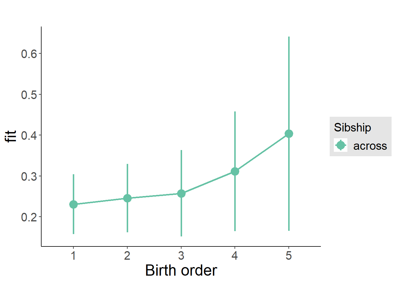
Add Interaction
Model Summary
m4_interaction = update(m3_birthorder_nonlinear, formula = . ~ . - birth_order_nonlinear - sibling_count + count_birth_order)
tidy(m4_interaction, conf.int = T, conf.level = 0.995)| effect | group | term | estimate | std.error | statistic | df | p.value | conf.low | conf.high |
|---|---|---|---|---|---|---|---|---|---|
| fixed | NA | (Intercept) | -5.445 | 1.32 | -4.126 | 3359 | 0.00003786 | -9.149 | -1.74 |
| fixed | NA | poly(age, 3, raw = TRUE)1 | 0.5654 | 0.2017 | 2.803 | 3333 | 0.005094 | -0.0008416 | 1.132 |
| fixed | NA | poly(age, 3, raw = TRUE)2 | -0.01592 | 0.01003 | -1.588 | 3316 | 0.1124 | -0.04407 | 0.01223 |
| fixed | NA | poly(age, 3, raw = TRUE)3 | 0.0001091 | 0.0001622 | 0.6726 | 3304 | 0.5012 | -0.0003463 | 0.0005645 |
| fixed | NA | male | -0.1383 | 0.02683 | -5.156 | 4077 | 0.0000002645 | -0.2136 | -0.06302 |
| fixed | NA | count_birth_order2/2 | 0.0294 | 0.04884 | 0.602 | 3287 | 0.5472 | -0.1077 | 0.1665 |
| fixed | NA | count_birth_order1/3 | 0.03419 | 0.04708 | 0.7262 | 4367 | 0.4678 | -0.09797 | 0.1664 |
| fixed | NA | count_birth_order2/3 | 0.05688 | 0.05113 | 1.112 | 4420 | 0.266 | -0.08665 | 0.2004 |
| fixed | NA | count_birth_order3/3 | 0.03759 | 0.05703 | 0.6592 | 4420 | 0.5098 | -0.1225 | 0.1977 |
| fixed | NA | count_birth_order1/4 | -0.07872 | 0.06328 | -1.244 | 4422 | 0.2136 | -0.2564 | 0.09892 |
| fixed | NA | count_birth_order2/4 | -0.06051 | 0.06314 | -0.9582 | 4382 | 0.338 | -0.2378 | 0.1167 |
| fixed | NA | count_birth_order3/4 | -0.02095 | 0.06578 | -0.3185 | 4290 | 0.7501 | -0.2056 | 0.1637 |
| fixed | NA | count_birth_order4/4 | 0.02731 | 0.06541 | 0.4176 | 4420 | 0.6763 | -0.1563 | 0.2109 |
| fixed | NA | count_birth_order1/5 | -0.09907 | 0.09546 | -1.038 | 4340 | 0.2994 | -0.367 | 0.1689 |
| fixed | NA | count_birth_order2/5 | -0.226 | 0.1006 | -2.247 | 4079 | 0.02468 | -0.5083 | 0.0563 |
| fixed | NA | count_birth_order3/5 | -0.1136 | 0.08865 | -1.282 | 4191 | 0.2 | -0.3624 | 0.1352 |
| fixed | NA | count_birth_order4/5 | -0.1012 | 0.08334 | -1.214 | 4294 | 0.2249 | -0.3351 | 0.1328 |
| fixed | NA | count_birth_order5/5 | 0.008885 | 0.08078 | 0.11 | 4407 | 0.9124 | -0.2179 | 0.2356 |
| ran_pars | mother_pidlink | sd__(Intercept) | 0.547 | NA | NA | NA | NA | NA | NA |
| ran_pars | Residual | sd__Observation | 0.7499 | NA | NA | NA | NA | NA | NA |
Coefficient Plot
plot_birthorder(m4_interaction)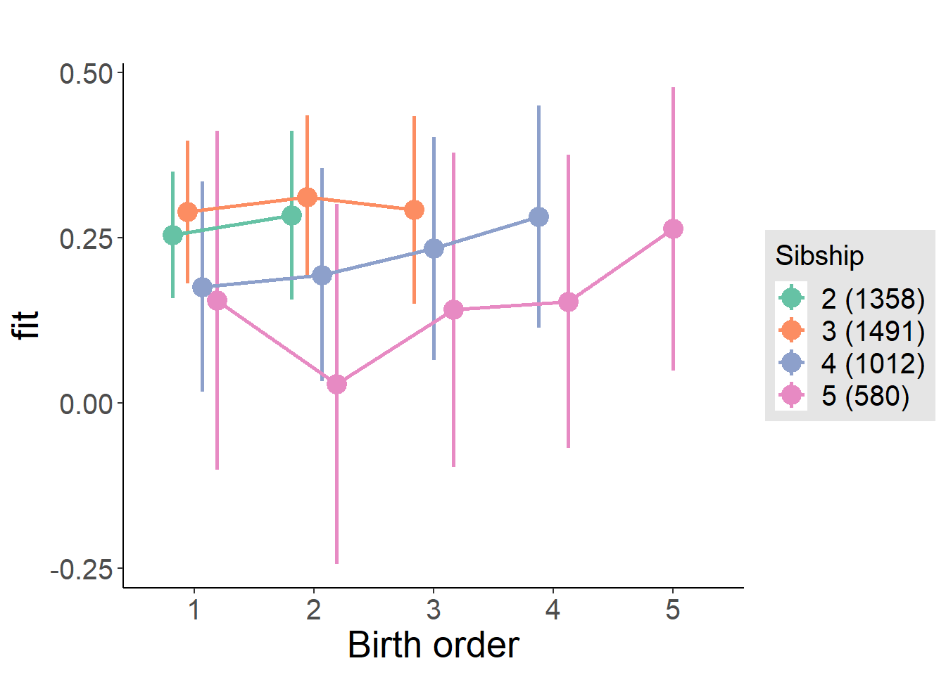
Model Comparison
###### Model 1 - Model 2
anova(m1_covariates_only, m2_birthorder_linear, m3_birthorder_nonlinear, m4_interaction)## refitting model(s) with ML (instead of REML)| Df | AIC | BIC | logLik | deviance | Chisq | Chi Df | Pr(>Chisq) |
|---|---|---|---|---|---|---|---|
| 10 | 11768 | 11832 | -5874 | 11748 | NA | NA | NA |
| 11 | 11767 | 11837 | -5872 | 11745 | 3.254 | 1 | 0.07124 |
| 14 | 11771 | 11861 | -5872 | 11743 | 1.351 | 3 | 0.717 |
| 20 | 11781 | 11909 | -5871 | 11741 | 2.092 | 6 | 0.911 |
Maternal pregnancy order
outcome_preg_m1 <- update(m2_birthorder_linear, data = birthorder %>%
mutate(sibling_count = sibling_count_uterus_preg_factor,
birth_order_nonlinear = birthorder_uterus_preg_factor,
birth_order = birthorder_uterus_preg,
count_birth_order = count_birthorder_uterus_preg
) %>%
filter(sibling_count != "1"))
compare_models_markdown(outcome_preg_m1)Basic Model
Model Summary
m1_covariates_only <- update(m2_birthorder_linear, formula = . ~ . - birth_order)
tidy(m1_covariates_only, conf.int = T, conf.level = 0.995)| effect | group | term | estimate | std.error | statistic | df | p.value | conf.low | conf.high |
|---|---|---|---|---|---|---|---|---|---|
| fixed | NA | (Intercept) | -5.346 | 1.357 | -3.94 | 3131 | 0.00008318 | -9.154 | -1.537 |
| fixed | NA | poly(age, 3, raw = TRUE)1 | 0.5626 | 0.2076 | 2.71 | 3110 | 0.006771 | -0.02021 | 1.145 |
| fixed | NA | poly(age, 3, raw = TRUE)2 | -0.01623 | 0.01033 | -1.57 | 3095 | 0.1165 | -0.04523 | 0.01278 |
| fixed | NA | poly(age, 3, raw = TRUE)3 | 0.0001208 | 0.0001674 | 0.7217 | 3082 | 0.4705 | -0.000349 | 0.0005906 |
| fixed | NA | male | -0.1475 | 0.02773 | -5.317 | 3815 | 0.0000001116 | -0.2253 | -0.06961 |
| fixed | NA | sibling_count3 | 0.01327 | 0.04009 | 0.3311 | 3023 | 0.7406 | -0.09927 | 0.1258 |
| fixed | NA | sibling_count4 | -0.05222 | 0.04372 | -1.194 | 2801 | 0.2324 | -0.175 | 0.0705 |
| fixed | NA | sibling_count5 | -0.07084 | 0.04945 | -1.433 | 2745 | 0.1521 | -0.2096 | 0.06797 |
| ran_pars | mother_pidlink | sd__(Intercept) | 0.5436 | NA | NA | NA | NA | NA | NA |
| ran_pars | Residual | sd__Observation | 0.7507 | NA | NA | NA | NA | NA | NA |
Coefficient Plot
plot(allEffects(m1_covariates_only, confidence.level = 0.995))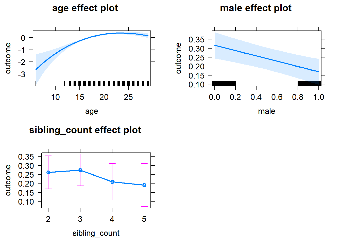
Add Birth Order Linear
Model Summary
tidy(m2_birthorder_linear, conf.int = T, conf.level = 0.995)| effect | group | term | estimate | std.error | statistic | df | p.value | conf.low | conf.high |
|---|---|---|---|---|---|---|---|---|---|
| fixed | NA | (Intercept) | -5.512 | 1.36 | -4.054 | 3135 | 0.00005157 | -9.329 | -1.696 |
| fixed | NA | birth_order | 0.02608 | 0.0147 | 1.774 | 4037 | 0.07607 | -0.01518 | 0.06734 |
| fixed | NA | poly(age, 3, raw = TRUE)1 | 0.5813 | 0.2079 | 2.797 | 3109 | 0.005195 | -0.00215 | 1.165 |
| fixed | NA | poly(age, 3, raw = TRUE)2 | -0.01711 | 0.01034 | -1.654 | 3092 | 0.09818 | -0.04615 | 0.01192 |
| fixed | NA | poly(age, 3, raw = TRUE)3 | 0.0001351 | 0.0001675 | 0.8062 | 3080 | 0.4202 | -0.0003352 | 0.0006053 |
| fixed | NA | male | -0.1482 | 0.02773 | -5.345 | 3815 | 0.00000009593 | -0.226 | -0.07037 |
| fixed | NA | sibling_count3 | 0.0003254 | 0.04074 | 0.007986 | 3056 | 0.9936 | -0.114 | 0.1147 |
| fixed | NA | sibling_count4 | -0.08131 | 0.04668 | -1.742 | 2970 | 0.08165 | -0.2123 | 0.04973 |
| fixed | NA | sibling_count5 | -0.1196 | 0.05655 | -2.114 | 3047 | 0.03456 | -0.2783 | 0.03917 |
| ran_pars | mother_pidlink | sd__(Intercept) | 0.5432 | NA | NA | NA | NA | NA | NA |
| ran_pars | Residual | sd__Observation | 0.7506 | NA | NA | NA | NA | NA | NA |
Coefficient Plot
plot_birthorder2(m2_birthorder_linear, separate = FALSE)
Add Birth Order Factor
Model Summary
m3_birthorder_nonlinear = update(m1_covariates_only, formula = . ~ . + birth_order_nonlinear)
tidy(m3_birthorder_nonlinear, conf.int = T, conf.level = 0.995)| effect | group | term | estimate | std.error | statistic | df | p.value | conf.low | conf.high |
|---|---|---|---|---|---|---|---|---|---|
| fixed | NA | (Intercept) | -5.504 | 1.361 | -4.045 | 3140 | 0.00005347 | -9.324 | -1.685 |
| fixed | NA | poly(age, 3, raw = TRUE)1 | 0.583 | 0.2081 | 2.801 | 3115 | 0.005123 | -0.001217 | 1.167 |
| fixed | NA | poly(age, 3, raw = TRUE)2 | -0.01718 | 0.01036 | -1.659 | 3098 | 0.0973 | -0.04625 | 0.01189 |
| fixed | NA | poly(age, 3, raw = TRUE)3 | 0.0001359 | 0.0001678 | 0.81 | 3086 | 0.418 | -0.000335 | 0.0006068 |
| fixed | NA | male | -0.1482 | 0.02775 | -5.339 | 3813 | 0.0000000987 | -0.2261 | -0.07027 |
| fixed | NA | sibling_count3 | 0.0004552 | 0.04133 | 0.01101 | 3152 | 0.9912 | -0.1156 | 0.1165 |
| fixed | NA | sibling_count4 | -0.07924 | 0.04738 | -1.672 | 3060 | 0.09459 | -0.2122 | 0.05377 |
| fixed | NA | sibling_count5 | -0.1162 | 0.05757 | -2.018 | 3068 | 0.04368 | -0.2778 | 0.04543 |
| fixed | NA | birth_order_nonlinear2 | 0.04271 | 0.03175 | 1.345 | 2872 | 0.1786 | -0.04641 | 0.1318 |
| fixed | NA | birth_order_nonlinear3 | 0.0513 | 0.0418 | 1.227 | 3413 | 0.2199 | -0.06605 | 0.1686 |
| fixed | NA | birth_order_nonlinear4 | 0.07387 | 0.05683 | 1.3 | 3696 | 0.1937 | -0.08565 | 0.2334 |
| fixed | NA | birth_order_nonlinear5 | 0.1039 | 0.08527 | 1.219 | 3863 | 0.2231 | -0.1354 | 0.3433 |
| ran_pars | mother_pidlink | sd__(Intercept) | 0.5426 | NA | NA | NA | NA | NA | NA |
| ran_pars | Residual | sd__Observation | 0.7513 | NA | NA | NA | NA | NA | NA |
Coefficient Plot
plot_birthorder(m3_birthorder_nonlinear, separate = FALSE)
Add Interaction
Model Summary
m4_interaction = update(m3_birthorder_nonlinear, formula = . ~ . - birth_order_nonlinear - sibling_count + count_birth_order)
tidy(m4_interaction, conf.int = T, conf.level = 0.995)| effect | group | term | estimate | std.error | statistic | df | p.value | conf.low | conf.high |
|---|---|---|---|---|---|---|---|---|---|
| fixed | NA | (Intercept) | -5.535 | 1.361 | -4.067 | 3139 | 0.00004877 | -9.355 | -1.715 |
| fixed | NA | poly(age, 3, raw = TRUE)1 | 0.587 | 0.2082 | 2.819 | 3115 | 0.004847 | 0.002501 | 1.171 |
| fixed | NA | poly(age, 3, raw = TRUE)2 | -0.01738 | 0.01036 | -1.678 | 3099 | 0.09354 | -0.04647 | 0.0117 |
| fixed | NA | poly(age, 3, raw = TRUE)3 | 0.0001395 | 0.0001678 | 0.8311 | 3087 | 0.406 | -0.0003316 | 0.0006106 |
| fixed | NA | male | -0.1471 | 0.02777 | -5.297 | 3810 | 0.0000001245 | -0.225 | -0.06914 |
| fixed | NA | count_birth_order2/2 | 0.05386 | 0.05366 | 1.004 | 3068 | 0.3156 | -0.09677 | 0.2045 |
| fixed | NA | count_birth_order1/3 | 0.01198 | 0.05073 | 0.2362 | 4089 | 0.8133 | -0.1304 | 0.1544 |
| fixed | NA | count_birth_order2/3 | 0.04961 | 0.05445 | 0.9111 | 4128 | 0.3623 | -0.1032 | 0.2024 |
| fixed | NA | count_birth_order3/3 | 0.03463 | 0.06114 | 0.5664 | 4124 | 0.5711 | -0.137 | 0.2062 |
| fixed | NA | count_birth_order1/4 | -0.112 | 0.06357 | -1.761 | 4129 | 0.07826 | -0.2904 | 0.06648 |
| fixed | NA | count_birth_order2/4 | -0.05171 | 0.0641 | -0.8068 | 4102 | 0.4198 | -0.2316 | 0.1282 |
| fixed | NA | count_birth_order3/4 | -0.04066 | 0.0673 | -0.6041 | 4022 | 0.5458 | -0.2296 | 0.1483 |
| fixed | NA | count_birth_order4/4 | 0.07804 | 0.06904 | 1.13 | 4122 | 0.2584 | -0.1158 | 0.2718 |
| fixed | NA | count_birth_order1/5 | -0.05507 | 0.08616 | -0.6392 | 4080 | 0.5227 | -0.2969 | 0.1868 |
| fixed | NA | count_birth_order2/5 | -0.06749 | 0.08712 | -0.7747 | 3984 | 0.4385 | -0.312 | 0.1771 |
| fixed | NA | count_birth_order3/5 | 0.01181 | 0.0831 | 0.1422 | 3966 | 0.8869 | -0.2214 | 0.2451 |
| fixed | NA | count_birth_order4/5 | -0.1652 | 0.08356 | -1.977 | 3939 | 0.04814 | -0.3997 | 0.06938 |
| fixed | NA | count_birth_order5/5 | -0.01713 | 0.08009 | -0.2139 | 4118 | 0.8307 | -0.242 | 0.2077 |
| ran_pars | mother_pidlink | sd__(Intercept) | 0.5424 | NA | NA | NA | NA | NA | NA |
| ran_pars | Residual | sd__Observation | 0.7512 | NA | NA | NA | NA | NA | NA |
Coefficient Plot
plot_birthorder(m4_interaction)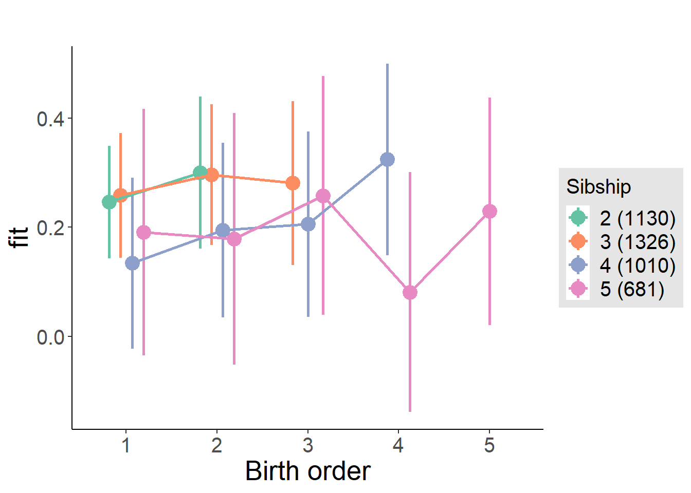
Model Comparison
###### Model 1 - Model 2
anova(m1_covariates_only, m2_birthorder_linear, m3_birthorder_nonlinear, m4_interaction)## refitting model(s) with ML (instead of REML)| Df | AIC | BIC | logLik | deviance | Chisq | Chi Df | Pr(>Chisq) |
|---|---|---|---|---|---|---|---|
| 10 | 10989 | 11052 | -5485 | 10969 | NA | NA | NA |
| 11 | 10988 | 11058 | -5483 | 10966 | 3.154 | 1 | 0.07572 |
| 14 | 10994 | 11082 | -5483 | 10966 | 0.3642 | 3 | 0.9475 |
| 20 | 10998 | 11125 | -5479 | 10958 | 7.449 | 6 | 0.2813 |
Parental full sibling order
outcome_parental_m1 <- update(m2_birthorder_linear, data = birthorder %>%
mutate(sibling_count = sibling_count_genes_factor,
birth_order_nonlinear = birthorder_genes_factor,
birth_order = birthorder_genes,
count_birth_order = count_birthorder_genes
) %>%
filter(sibling_count != "1"))
compare_models_markdown(outcome_parental_m1)Basic Model
Model Summary
m1_covariates_only <- update(m2_birthorder_linear, formula = . ~ . - birth_order)
tidy(m1_covariates_only, conf.int = T, conf.level = 0.995)| effect | group | term | estimate | std.error | statistic | df | p.value | conf.low | conf.high |
|---|---|---|---|---|---|---|---|---|---|
| fixed | NA | (Intercept) | -5.242 | 1.327 | -3.952 | 3280 | 0.00007928 | -8.966 | -1.518 |
| fixed | NA | poly(age, 3, raw = TRUE)1 | 0.5305 | 0.2028 | 2.616 | 3260 | 0.008937 | -0.03873 | 1.1 |
| fixed | NA | poly(age, 3, raw = TRUE)2 | -0.01401 | 0.01008 | -1.39 | 3245 | 0.1648 | -0.0423 | 0.01429 |
| fixed | NA | poly(age, 3, raw = TRUE)3 | 0.00007446 | 0.000163 | 0.4567 | 3233 | 0.6479 | -0.0003832 | 0.0005321 |
| fixed | NA | male | -0.1405 | 0.02702 | -5.199 | 4002 | 0.0000002102 | -0.2164 | -0.06464 |
| fixed | NA | sibling_count3 | 0.06438 | 0.03744 | 1.719 | 3104 | 0.08564 | -0.04072 | 0.1695 |
| fixed | NA | sibling_count4 | -0.01646 | 0.04261 | -0.3864 | 2836 | 0.6992 | -0.1361 | 0.1031 |
| fixed | NA | sibling_count5 | -0.123 | 0.0533 | -2.308 | 2761 | 0.02107 | -0.2726 | 0.02659 |
| ran_pars | mother_pidlink | sd__(Intercept) | 0.5523 | NA | NA | NA | NA | NA | NA |
| ran_pars | Residual | sd__Observation | 0.7505 | NA | NA | NA | NA | NA | NA |
Coefficient Plot
plot(allEffects(m1_covariates_only, confidence.level = 0.995))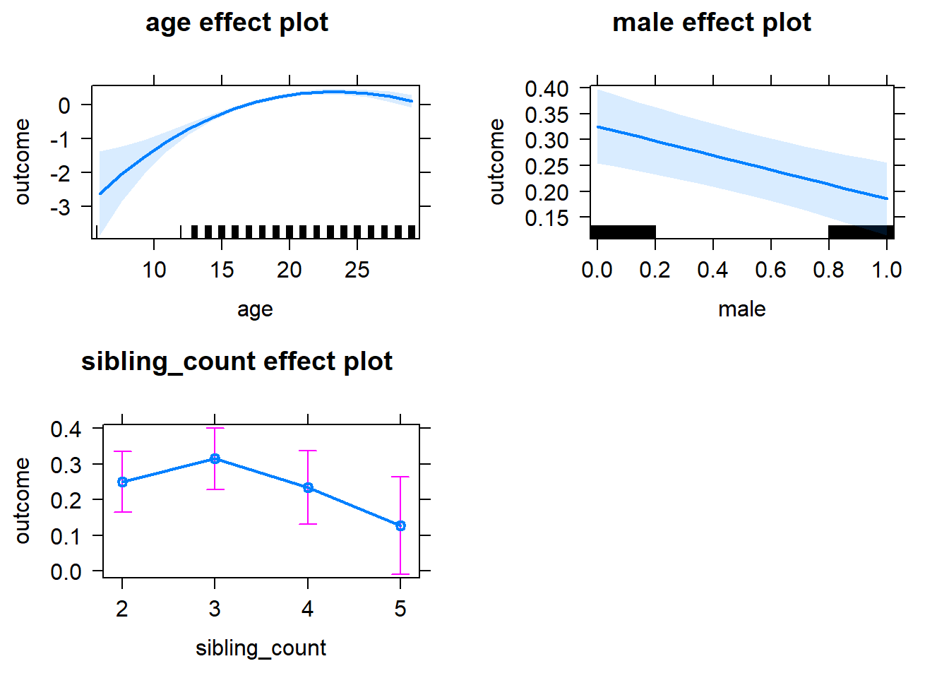
Add Birth Order Linear
Model Summary
tidy(m2_birthorder_linear, conf.int = T, conf.level = 0.995)| effect | group | term | estimate | std.error | statistic | df | p.value | conf.low | conf.high |
|---|---|---|---|---|---|---|---|---|---|
| fixed | NA | (Intercept) | -5.43 | 1.33 | -4.081 | 3285 | 0.00004586 | -9.164 | -1.695 |
| fixed | NA | birth_order | 0.02734 | 0.01495 | 1.828 | 4178 | 0.06759 | -0.01464 | 0.06931 |
| fixed | NA | poly(age, 3, raw = TRUE)1 | 0.552 | 0.2031 | 2.718 | 3258 | 0.006606 | -0.01812 | 1.122 |
| fixed | NA | poly(age, 3, raw = TRUE)2 | -0.01502 | 0.01009 | -1.488 | 3241 | 0.1368 | -0.04336 | 0.01331 |
| fixed | NA | poly(age, 3, raw = TRUE)3 | 0.00009068 | 0.0001633 | 0.5555 | 3230 | 0.5786 | -0.0003676 | 0.000549 |
| fixed | NA | male | -0.1411 | 0.02702 | -5.221 | 4002 | 0.0000001865 | -0.2169 | -0.06524 |
| fixed | NA | sibling_count3 | 0.05143 | 0.03809 | 1.35 | 3148 | 0.1771 | -0.05549 | 0.1584 |
| fixed | NA | sibling_count4 | -0.04907 | 0.04618 | -1.063 | 3054 | 0.2881 | -0.1787 | 0.08055 |
| fixed | NA | sibling_count5 | -0.1771 | 0.06093 | -2.906 | 3137 | 0.003685 | -0.3481 | -0.00604 |
| ran_pars | mother_pidlink | sd__(Intercept) | 0.5517 | NA | NA | NA | NA | NA | NA |
| ran_pars | Residual | sd__Observation | 0.7505 | NA | NA | NA | NA | NA | NA |
Coefficient Plot
plot_birthorder2(m2_birthorder_linear, separate = FALSE)
Add Birth Order Factor
Model Summary
m3_birthorder_nonlinear = update(m1_covariates_only, formula = . ~ . + birth_order_nonlinear)
tidy(m3_birthorder_nonlinear, conf.int = T, conf.level = 0.995)| effect | group | term | estimate | std.error | statistic | df | p.value | conf.low | conf.high |
|---|---|---|---|---|---|---|---|---|---|
| fixed | NA | (Intercept) | -5.412 | 1.332 | -4.064 | 3290 | 0.00004943 | -9.15 | -1.674 |
| fixed | NA | poly(age, 3, raw = TRUE)1 | 0.5542 | 0.2034 | 2.724 | 3264 | 0.006485 | -0.01691 | 1.125 |
| fixed | NA | poly(age, 3, raw = TRUE)2 | -0.01515 | 0.01011 | -1.498 | 3247 | 0.1342 | -0.04353 | 0.01323 |
| fixed | NA | poly(age, 3, raw = TRUE)3 | 0.00009293 | 0.0001635 | 0.5683 | 3236 | 0.5699 | -0.0003661 | 0.000552 |
| fixed | NA | male | -0.1411 | 0.02704 | -5.218 | 4000 | 0.0000001896 | -0.217 | -0.0652 |
| fixed | NA | sibling_count3 | 0.05318 | 0.03869 | 1.374 | 3261 | 0.1694 | -0.05544 | 0.1618 |
| fixed | NA | sibling_count4 | -0.04646 | 0.047 | -0.9885 | 3152 | 0.323 | -0.1784 | 0.08548 |
| fixed | NA | sibling_count5 | -0.1868 | 0.06315 | -2.959 | 3220 | 0.003111 | -0.3641 | -0.009586 |
| fixed | NA | birth_order_nonlinear2 | 0.01922 | 0.03043 | 0.6316 | 2936 | 0.5277 | -0.06621 | 0.1046 |
| fixed | NA | birth_order_nonlinear3 | 0.0465 | 0.04127 | 1.127 | 3477 | 0.2599 | -0.06935 | 0.1623 |
| fixed | NA | birth_order_nonlinear4 | 0.07684 | 0.05765 | 1.333 | 3890 | 0.1826 | -0.08498 | 0.2387 |
| fixed | NA | birth_order_nonlinear5 | 0.1511 | 0.0942 | 1.604 | 3934 | 0.1089 | -0.1134 | 0.4155 |
| ran_pars | mother_pidlink | sd__(Intercept) | 0.5511 | NA | NA | NA | NA | NA | NA |
| ran_pars | Residual | sd__Observation | 0.7512 | NA | NA | NA | NA | NA | NA |
Coefficient Plot
plot_birthorder(m3_birthorder_nonlinear, separate = FALSE)
Add Interaction
Model Summary
m4_interaction = update(m3_birthorder_nonlinear, formula = . ~ . - birth_order_nonlinear - sibling_count + count_birth_order)
tidy(m4_interaction, conf.int = T, conf.level = 0.995)| effect | group | term | estimate | std.error | statistic | df | p.value | conf.low | conf.high |
|---|---|---|---|---|---|---|---|---|---|
| fixed | NA | (Intercept) | -5.423 | 1.333 | -4.069 | 3290 | 0.00004824 | -9.164 | -1.682 |
| fixed | NA | poly(age, 3, raw = TRUE)1 | 0.5548 | 0.2036 | 2.724 | 3265 | 0.006475 | -0.01681 | 1.126 |
| fixed | NA | poly(age, 3, raw = TRUE)2 | -0.01518 | 0.01012 | -1.5 | 3247 | 0.1338 | -0.04358 | 0.01323 |
| fixed | NA | poly(age, 3, raw = TRUE)3 | 0.00009353 | 0.0001637 | 0.5715 | 3235 | 0.5677 | -0.0003659 | 0.0005529 |
| fixed | NA | male | -0.1395 | 0.02708 | -5.15 | 3998 | 0.0000002728 | -0.2155 | -0.06345 |
| fixed | NA | count_birth_order2/2 | 0.0389 | 0.04784 | 0.8132 | 3175 | 0.4162 | -0.09539 | 0.1732 |
| fixed | NA | count_birth_order1/3 | 0.06461 | 0.0471 | 1.372 | 4305 | 0.1702 | -0.06759 | 0.1968 |
| fixed | NA | count_birth_order2/3 | 0.09009 | 0.05176 | 1.74 | 4355 | 0.08184 | -0.0552 | 0.2354 |
| fixed | NA | count_birth_order3/3 | 0.08117 | 0.05723 | 1.418 | 4353 | 0.1562 | -0.07949 | 0.2418 |
| fixed | NA | count_birth_order1/4 | -0.0743 | 0.06432 | -1.155 | 4357 | 0.2481 | -0.2548 | 0.1063 |
| fixed | NA | count_birth_order2/4 | -0.03049 | 0.0637 | -0.4787 | 4318 | 0.6322 | -0.2093 | 0.1483 |
| fixed | NA | count_birth_order3/4 | 0.02953 | 0.06606 | 0.447 | 4212 | 0.6549 | -0.1559 | 0.215 |
| fixed | NA | count_birth_order4/4 | 0.06093 | 0.0657 | 0.9274 | 4356 | 0.3538 | -0.1235 | 0.2453 |
| fixed | NA | count_birth_order1/5 | -0.05863 | 0.09712 | -0.6037 | 4292 | 0.5461 | -0.3312 | 0.214 |
| fixed | NA | count_birth_order2/5 | -0.2847 | 0.1072 | -2.657 | 3971 | 0.007918 | -0.5855 | 0.01609 |
| fixed | NA | count_birth_order3/5 | -0.1085 | 0.09332 | -1.163 | 4122 | 0.2449 | -0.3705 | 0.1534 |
| fixed | NA | count_birth_order4/5 | -0.151 | 0.08812 | -1.714 | 4201 | 0.08667 | -0.3984 | 0.09636 |
| fixed | NA | count_birth_order5/5 | -0.03391 | 0.086 | -0.3942 | 4341 | 0.6934 | -0.2753 | 0.2075 |
| ran_pars | mother_pidlink | sd__(Intercept) | 0.5511 | NA | NA | NA | NA | NA | NA |
| ran_pars | Residual | sd__Observation | 0.7512 | NA | NA | NA | NA | NA | NA |
Coefficient Plot
plot_birthorder(m4_interaction)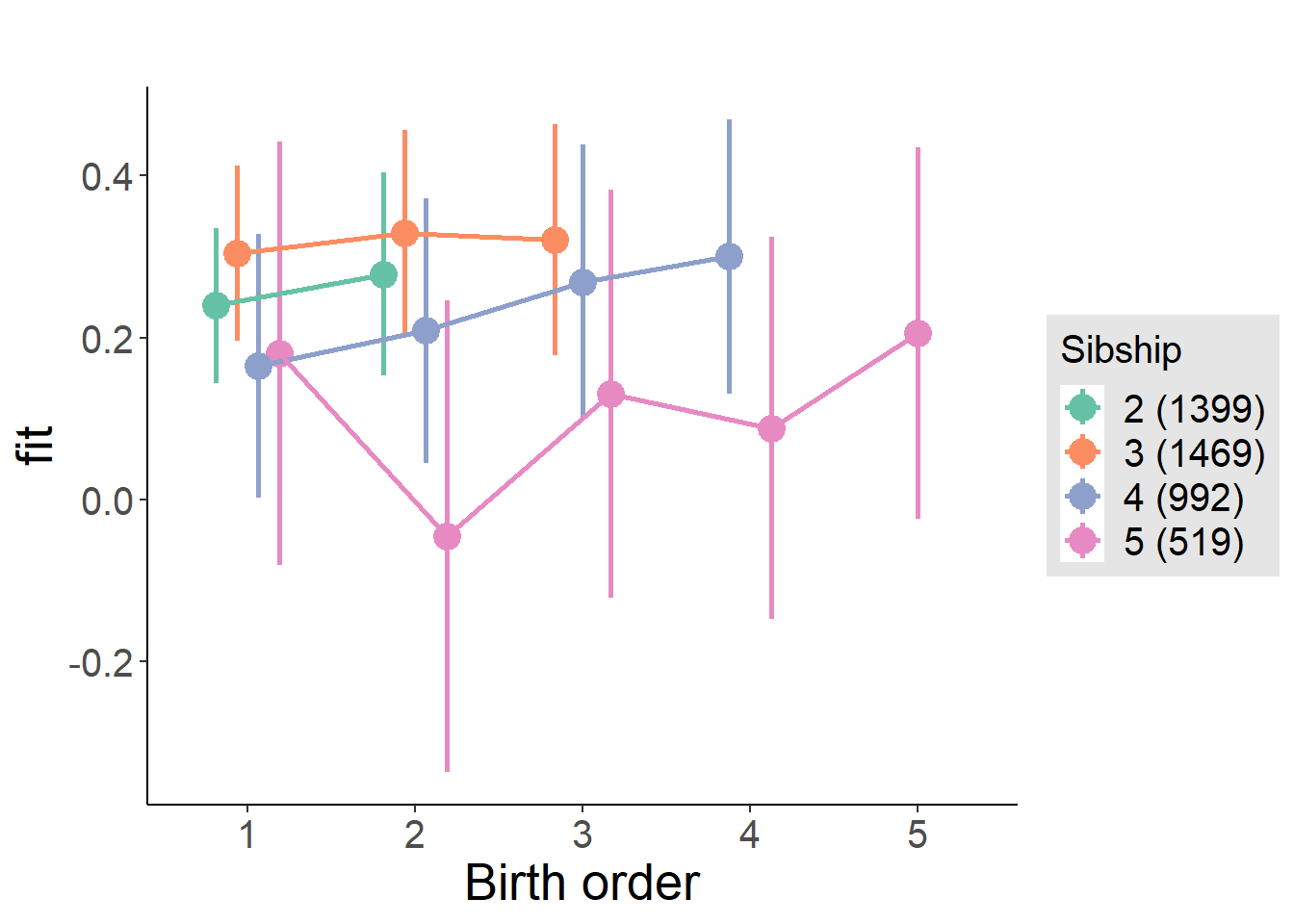
Model Comparison
###### Model 1 - Model 2
anova(m1_covariates_only, m2_birthorder_linear, m3_birthorder_nonlinear, m4_interaction)## refitting model(s) with ML (instead of REML)| Df | AIC | BIC | logLik | deviance | Chisq | Chi Df | Pr(>Chisq) |
|---|---|---|---|---|---|---|---|
| 10 | 11635 | 11698 | -5807 | 11615 | NA | NA | NA |
| 11 | 11633 | 11704 | -5806 | 11611 | 3.348 | 1 | 0.06728 |
| 14 | 11639 | 11728 | -5805 | 11611 | 0.3631 | 3 | 0.9478 |
| 20 | 11646 | 11773 | -5803 | 11606 | 5.416 | 6 | 0.4916 |
Compare birth order specifications
library(coefplot)
multiplot(outcome_naive_m1, outcome_preg_m1, outcome_uterus_m1, outcome_parental_m1, dodgeHeight = 0.6,
intercept = FALSE)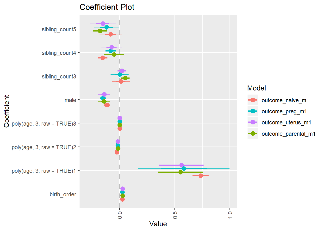
Counting backwards
birthorder <- birthorder %>% mutate(outcome = count_backwards)
model = lmer(outcome ~ birth_order + poly(age, 3, raw = TRUE) + male + sibling_count + (1 | mother_pidlink),
data = birthorder)
compare_birthorder_specs(model)Naive birth order
outcome_naive_m1 <- update(m2_birthorder_linear, data = birthorder %>%
mutate(sibling_count = sibling_count_naive_factor,
birth_order_nonlinear = birthorder_naive_factor,
birth_order = birthorder_naive,
count_birth_order = count_birthorder_naive) %>%
filter(sibling_count != "1"))
compare_models_markdown(outcome_naive_m1)Basic Model
Model Summary
m1_covariates_only <- update(m2_birthorder_linear, formula = . ~ . - birth_order)
tidy(m1_covariates_only, conf.int = T, conf.level = 0.995)| effect | group | term | estimate | std.error | statistic | df | p.value | conf.low | conf.high |
|---|---|---|---|---|---|---|---|---|---|
| fixed | NA | (Intercept) | -0.7392 | 0.1991 | -3.714 | 6789 | 0.000206 | -1.298 | -0.1804 |
| fixed | NA | poly(age, 3, raw = TRUE)1 | 0.09312 | 0.01916 | 4.86 | 6683 | 0.000001198 | 0.03934 | 0.1469 |
| fixed | NA | poly(age, 3, raw = TRUE)2 | -0.003023 | 0.0005607 | -5.392 | 6539 | 0.00000007214 | -0.004597 | -0.001449 |
| fixed | NA | poly(age, 3, raw = TRUE)3 | 0.0000272 | 0.000005094 | 5.339 | 6410 | 0.0000000965 | 0.0000129 | 0.0000415 |
| fixed | NA | male | 0.03845 | 0.02283 | 1.684 | 6721 | 0.09216 | -0.02563 | 0.1025 |
| fixed | NA | sibling_count3 | -0.002074 | 0.034 | -0.06101 | 4888 | 0.9514 | -0.09751 | 0.09336 |
| fixed | NA | sibling_count4 | 0.02362 | 0.03528 | 0.6695 | 4440 | 0.5032 | -0.0754 | 0.1226 |
| fixed | NA | sibling_count5 | 0.004105 | 0.03678 | 0.1116 | 4000 | 0.9111 | -0.09913 | 0.1073 |
| ran_pars | mother_pidlink | sd__(Intercept) | 0.4316 | NA | NA | NA | NA | NA | NA |
| ran_pars | Residual | sd__Observation | 0.871 | NA | NA | NA | NA | NA | NA |
Coefficient Plot
plot(allEffects(m1_covariates_only, confidence.level = 0.995))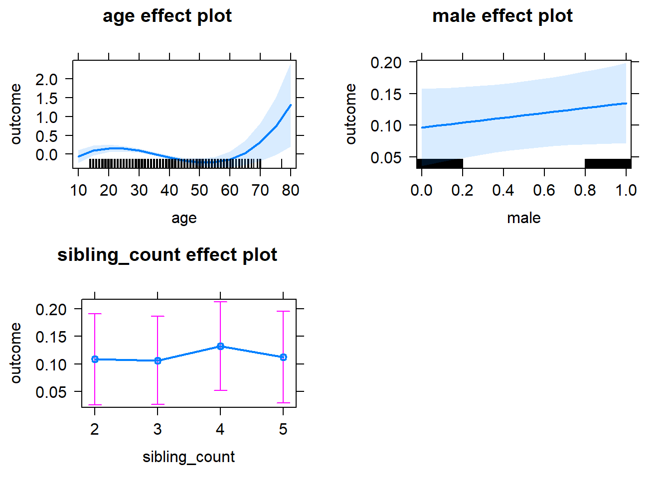
Add Birth Order Linear
Model Summary
tidy(m2_birthorder_linear, conf.int = T, conf.level = 0.995)| effect | group | term | estimate | std.error | statistic | df | p.value | conf.low | conf.high |
|---|---|---|---|---|---|---|---|---|---|
| fixed | NA | (Intercept) | -0.7214 | 0.1991 | -3.624 | 6779 | 0.0002922 | -1.28 | -0.1626 |
| fixed | NA | birth_order | -0.03413 | 0.01121 | -3.043 | 5683 | 0.002351 | -0.06561 | -0.002648 |
| fixed | NA | poly(age, 3, raw = TRUE)1 | 0.0962 | 0.01918 | 5.016 | 6708 | 0.0000005408 | 0.04237 | 0.15 |
| fixed | NA | poly(age, 3, raw = TRUE)2 | -0.003105 | 0.0005612 | -5.533 | 6556 | 0.00000003262 | -0.00468 | -0.00153 |
| fixed | NA | poly(age, 3, raw = TRUE)3 | 0.00002773 | 0.000005095 | 5.442 | 6423 | 0.00000005465 | 0.00001343 | 0.00004203 |
| fixed | NA | male | 0.03942 | 0.02281 | 1.728 | 6713 | 0.08403 | -0.02461 | 0.1035 |
| fixed | NA | sibling_count3 | 0.009728 | 0.03422 | 0.2843 | 4998 | 0.7762 | -0.08632 | 0.1058 |
| fixed | NA | sibling_count4 | 0.05173 | 0.03647 | 1.418 | 4924 | 0.1561 | -0.05064 | 0.1541 |
| fixed | NA | sibling_count5 | 0.04923 | 0.03966 | 1.241 | 4958 | 0.2146 | -0.0621 | 0.1606 |
| ran_pars | mother_pidlink | sd__(Intercept) | 0.4337 | NA | NA | NA | NA | NA | NA |
| ran_pars | Residual | sd__Observation | 0.8695 | NA | NA | NA | NA | NA | NA |
Coefficient Plot
plot_birthorder2(m2_birthorder_linear, separate = FALSE)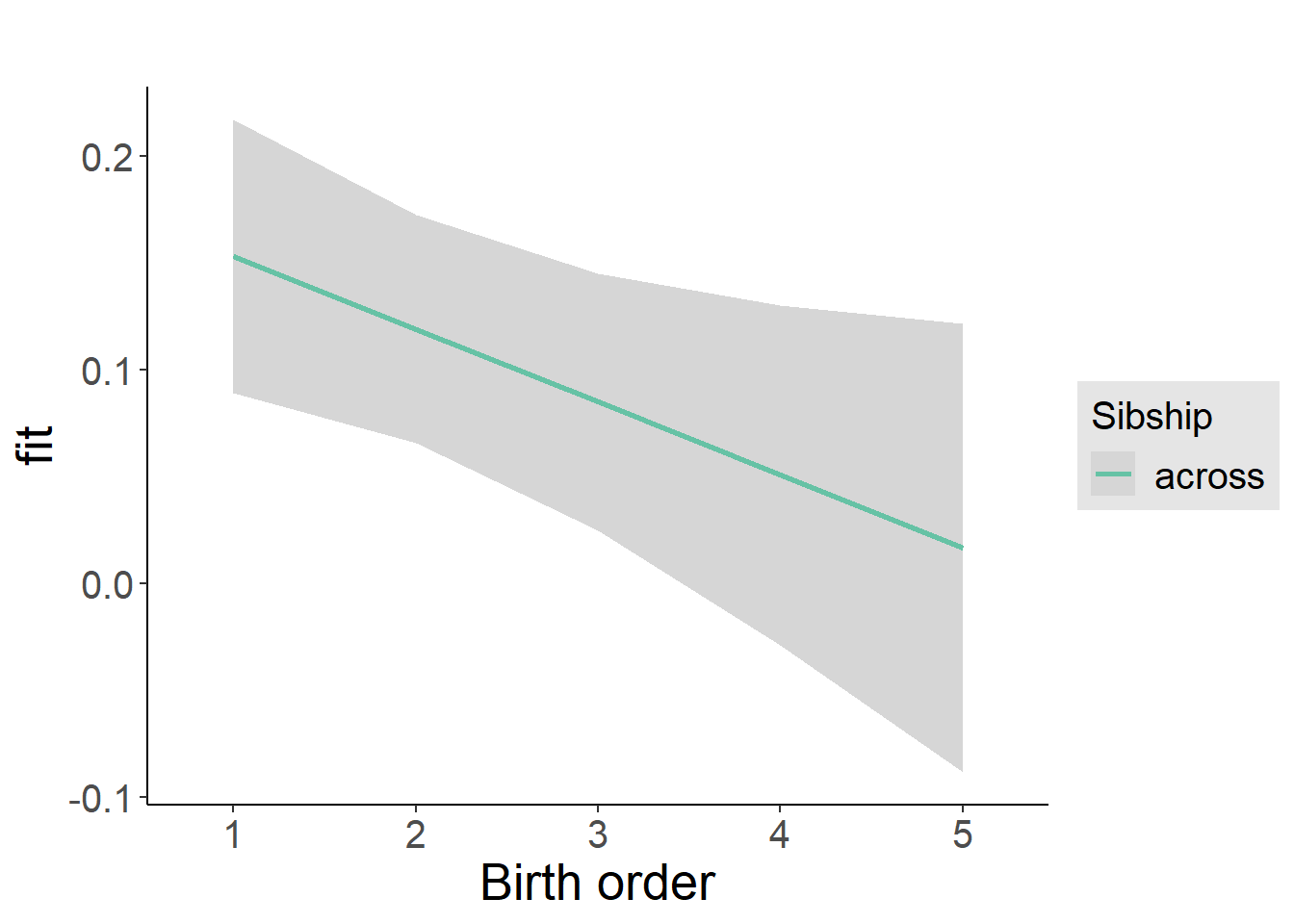
Add Birth Order Factor
Model Summary
m3_birthorder_nonlinear = update(m1_covariates_only, formula = . ~ . + birth_order_nonlinear)
tidy(m3_birthorder_nonlinear, conf.int = T, conf.level = 0.995)| effect | group | term | estimate | std.error | statistic | df | p.value | conf.low | conf.high |
|---|---|---|---|---|---|---|---|---|---|
| fixed | NA | (Intercept) | -0.7553 | 0.1995 | -3.786 | 6792 | 0.0001546 | -1.315 | -0.1953 |
| fixed | NA | poly(age, 3, raw = TRUE)1 | 0.09605 | 0.01919 | 5.005 | 6692 | 0.0000005729 | 0.04218 | 0.1499 |
| fixed | NA | poly(age, 3, raw = TRUE)2 | -0.003095 | 0.0005617 | -5.51 | 6530 | 0.00000003725 | -0.004672 | -0.001518 |
| fixed | NA | poly(age, 3, raw = TRUE)3 | 0.00002759 | 0.000005103 | 5.407 | 6383 | 0.00000006636 | 0.00001327 | 0.00004192 |
| fixed | NA | male | 0.0395 | 0.02281 | 1.731 | 6711 | 0.08346 | -0.02454 | 0.1035 |
| fixed | NA | sibling_count3 | 0.01763 | 0.03468 | 0.5083 | 5186 | 0.6113 | -0.07972 | 0.115 |
| fixed | NA | sibling_count4 | 0.0575 | 0.03699 | 1.555 | 5134 | 0.1201 | -0.04633 | 0.1613 |
| fixed | NA | sibling_count5 | 0.04835 | 0.03996 | 1.21 | 5102 | 0.2263 | -0.06382 | 0.1605 |
| fixed | NA | birth_order_nonlinear2 | -0.03516 | 0.02673 | -1.315 | 5658 | 0.1885 | -0.1102 | 0.03988 |
| fixed | NA | birth_order_nonlinear3 | -0.1045 | 0.03421 | -3.056 | 5479 | 0.002257 | -0.2006 | -0.008503 |
| fixed | NA | birth_order_nonlinear4 | -0.09262 | 0.04459 | -2.077 | 5422 | 0.03782 | -0.2178 | 0.03253 |
| fixed | NA | birth_order_nonlinear5 | -0.09832 | 0.06457 | -1.523 | 5225 | 0.1279 | -0.2796 | 0.08294 |
| ran_pars | mother_pidlink | sd__(Intercept) | 0.4331 | NA | NA | NA | NA | NA | NA |
| ran_pars | Residual | sd__Observation | 0.8698 | NA | NA | NA | NA | NA | NA |
Coefficient Plot
plot_birthorder(m3_birthorder_nonlinear, separate = FALSE)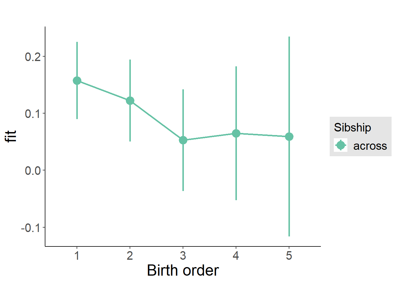
Add Interaction
Model Summary
m4_interaction = update(m3_birthorder_nonlinear, formula = . ~ . - birth_order_nonlinear - sibling_count + count_birth_order)
tidy(m4_interaction, conf.int = T, conf.level = 0.995)| effect | group | term | estimate | std.error | statistic | df | p.value | conf.low | conf.high |
|---|---|---|---|---|---|---|---|---|---|
| fixed | NA | (Intercept) | -0.7543 | 0.1998 | -3.774 | 6793 | 0.0001617 | -1.315 | -0.1933 |
| fixed | NA | poly(age, 3, raw = TRUE)1 | 0.09604 | 0.01919 | 5.005 | 6691 | 0.0000005728 | 0.04218 | 0.1499 |
| fixed | NA | poly(age, 3, raw = TRUE)2 | -0.003087 | 0.0005617 | -5.496 | 6527 | 0.00000004033 | -0.004663 | -0.00151 |
| fixed | NA | poly(age, 3, raw = TRUE)3 | 0.00002746 | 0.000005103 | 5.381 | 6377 | 0.00000007683 | 0.00001313 | 0.00004178 |
| fixed | NA | male | 0.04028 | 0.02281 | 1.766 | 6701 | 0.07749 | -0.02376 | 0.1043 |
| fixed | NA | count_birth_order2/2 | -0.04647 | 0.04579 | -1.015 | 5745 | 0.3102 | -0.175 | 0.08206 |
| fixed | NA | count_birth_order1/3 | 0.03489 | 0.04414 | 0.7904 | 6927 | 0.4293 | -0.08902 | 0.1588 |
| fixed | NA | count_birth_order2/3 | -0.0248 | 0.04917 | -0.5045 | 6980 | 0.6139 | -0.1628 | 0.1132 |
| fixed | NA | count_birth_order3/3 | -0.132 | 0.05508 | -2.397 | 6985 | 0.01656 | -0.2866 | 0.0226 |
| fixed | NA | count_birth_order1/4 | 0.07574 | 0.05051 | 1.499 | 6981 | 0.1338 | -0.06606 | 0.2175 |
| fixed | NA | count_birth_order2/4 | -0.001802 | 0.053 | -0.03399 | 6989 | 0.9729 | -0.1506 | 0.147 |
| fixed | NA | count_birth_order3/4 | -0.07465 | 0.05727 | -1.303 | 6978 | 0.1925 | -0.2354 | 0.08611 |
| fixed | NA | count_birth_order4/4 | -0.022 | 0.06047 | -0.3639 | 6960 | 0.7159 | -0.1917 | 0.1477 |
| fixed | NA | count_birth_order1/5 | -0.04515 | 0.05674 | -0.7957 | 6988 | 0.4262 | -0.2044 | 0.1141 |
| fixed | NA | count_birth_order2/5 | 0.05356 | 0.05969 | 0.8973 | 6971 | 0.3696 | -0.114 | 0.2211 |
| fixed | NA | count_birth_order3/5 | 0.02089 | 0.06146 | 0.3399 | 6951 | 0.7339 | -0.1516 | 0.1934 |
| fixed | NA | count_birth_order4/5 | -0.07004 | 0.06499 | -1.078 | 6915 | 0.2812 | -0.2525 | 0.1124 |
| fixed | NA | count_birth_order5/5 | -0.05243 | 0.06614 | -0.7927 | 6904 | 0.428 | -0.2381 | 0.1332 |
| ran_pars | mother_pidlink | sd__(Intercept) | 0.4338 | NA | NA | NA | NA | NA | NA |
| ran_pars | Residual | sd__Observation | 0.8693 | NA | NA | NA | NA | NA | NA |
Coefficient Plot
plot_birthorder(m4_interaction)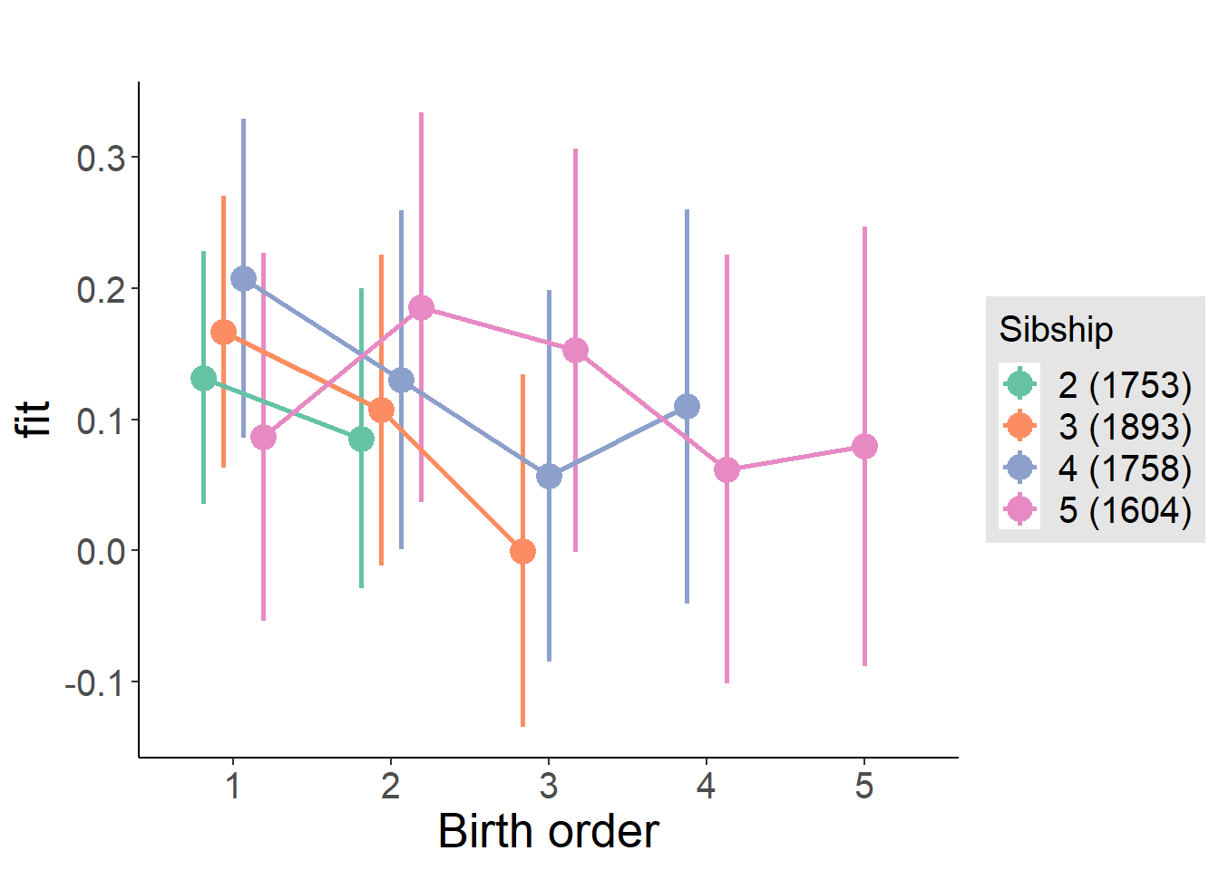
Model Comparison
###### Model 1 - Model 2
anova(m1_covariates_only, m2_birthorder_linear, m3_birthorder_nonlinear, m4_interaction)## refitting model(s) with ML (instead of REML)| Df | AIC | BIC | logLik | deviance | Chisq | Chi Df | Pr(>Chisq) |
|---|---|---|---|---|---|---|---|
| 10 | 19384 | 19453 | -9682 | 19364 | NA | NA | NA |
| 11 | 19377 | 19453 | -9678 | 19355 | 9.247 | 1 | 0.002359 |
| 14 | 19381 | 19477 | -9677 | 19353 | 2.051 | 3 | 0.5618 |
| 20 | 19384 | 19521 | -9672 | 19344 | 9.481 | 6 | 0.1483 |
Maternal birth order
outcome_uterus_m1 <- update(m2_birthorder_linear, data = birthorder %>%
mutate(sibling_count = sibling_count_uterus_alive_factor,
birth_order_nonlinear = birthorder_uterus_alive_factor,
birth_order = birthorder_uterus_alive,
count_birth_order = count_birthorder_uterus_alive) %>%
filter(sibling_count != "1"))
compare_models_markdown(outcome_uterus_m1)Basic Model
Model Summary
m1_covariates_only <- update(m2_birthorder_linear, formula = . ~ . - birth_order)
tidy(m1_covariates_only, conf.int = T, conf.level = 0.995)| effect | group | term | estimate | std.error | statistic | df | p.value | conf.low | conf.high |
|---|---|---|---|---|---|---|---|---|---|
| fixed | NA | (Intercept) | -1.723 | 0.4969 | -3.467 | 4434 | 0.0005318 | -3.117 | -0.3278 |
| fixed | NA | poly(age, 3, raw = TRUE)1 | 0.2051 | 0.05798 | 3.538 | 4440 | 0.0004076 | 0.04237 | 0.3679 |
| fixed | NA | poly(age, 3, raw = TRUE)2 | -0.006628 | 0.002137 | -3.102 | 4445 | 0.001934 | -0.01263 | -0.0006305 |
| fixed | NA | poly(age, 3, raw = TRUE)3 | 0.00006633 | 0.00002503 | 2.649 | 4448 | 0.00809 | -0.000003944 | 0.0001366 |
| fixed | NA | male | -0.006547 | 0.0267 | -0.2452 | 4306 | 0.8063 | -0.0815 | 0.06841 |
| fixed | NA | sibling_count3 | -0.007674 | 0.03723 | -0.2061 | 3153 | 0.8367 | -0.1122 | 0.09684 |
| fixed | NA | sibling_count4 | -0.0271 | 0.04045 | -0.67 | 2772 | 0.5029 | -0.1406 | 0.08644 |
| fixed | NA | sibling_count5 | -0.0746 | 0.04619 | -1.615 | 2502 | 0.1064 | -0.2043 | 0.05506 |
| ran_pars | mother_pidlink | sd__(Intercept) | 0.3812 | NA | NA | NA | NA | NA | NA |
| ran_pars | Residual | sd__Observation | 0.8173 | NA | NA | NA | NA | NA | NA |
Coefficient Plot
plot(allEffects(m1_covariates_only, confidence.level = 0.995))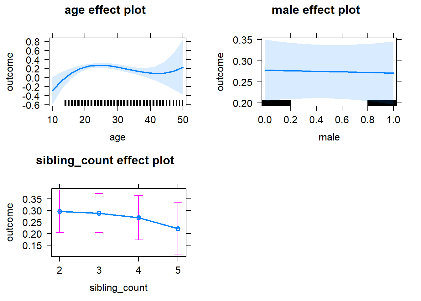
Add Birth Order Linear
Model Summary
tidy(m2_birthorder_linear, conf.int = T, conf.level = 0.995)| effect | group | term | estimate | std.error | statistic | df | p.value | conf.low | conf.high |
|---|---|---|---|---|---|---|---|---|---|
| fixed | NA | (Intercept) | -1.709 | 0.4975 | -3.435 | 4433 | 0.0005984 | -3.105 | -0.3123 |
| fixed | NA | birth_order | -0.008166 | 0.01393 | -0.586 | 3998 | 0.5579 | -0.04728 | 0.03095 |
| fixed | NA | poly(age, 3, raw = TRUE)1 | 0.2047 | 0.05799 | 3.53 | 4438 | 0.0004204 | 0.0419 | 0.3675 |
| fixed | NA | poly(age, 3, raw = TRUE)2 | -0.006604 | 0.002137 | -3.09 | 4443 | 0.002015 | -0.0126 | -0.0006044 |
| fixed | NA | poly(age, 3, raw = TRUE)3 | 0.00006587 | 0.00002505 | 2.63 | 4446 | 0.008571 | -0.000004438 | 0.0001362 |
| fixed | NA | male | -0.006218 | 0.02671 | -0.2328 | 4304 | 0.8159 | -0.08119 | 0.06875 |
| fixed | NA | sibling_count3 | -0.003895 | 0.0378 | -0.103 | 3214 | 0.9179 | -0.11 | 0.1022 |
| fixed | NA | sibling_count4 | -0.01835 | 0.04314 | -0.4253 | 2995 | 0.6707 | -0.1394 | 0.1027 |
| fixed | NA | sibling_count5 | -0.06005 | 0.05247 | -1.144 | 3011 | 0.2525 | -0.2073 | 0.08724 |
| ran_pars | mother_pidlink | sd__(Intercept) | 0.3821 | NA | NA | NA | NA | NA | NA |
| ran_pars | Residual | sd__Observation | 0.817 | NA | NA | NA | NA | NA | NA |
Coefficient Plot
plot_birthorder2(m2_birthorder_linear, separate = FALSE)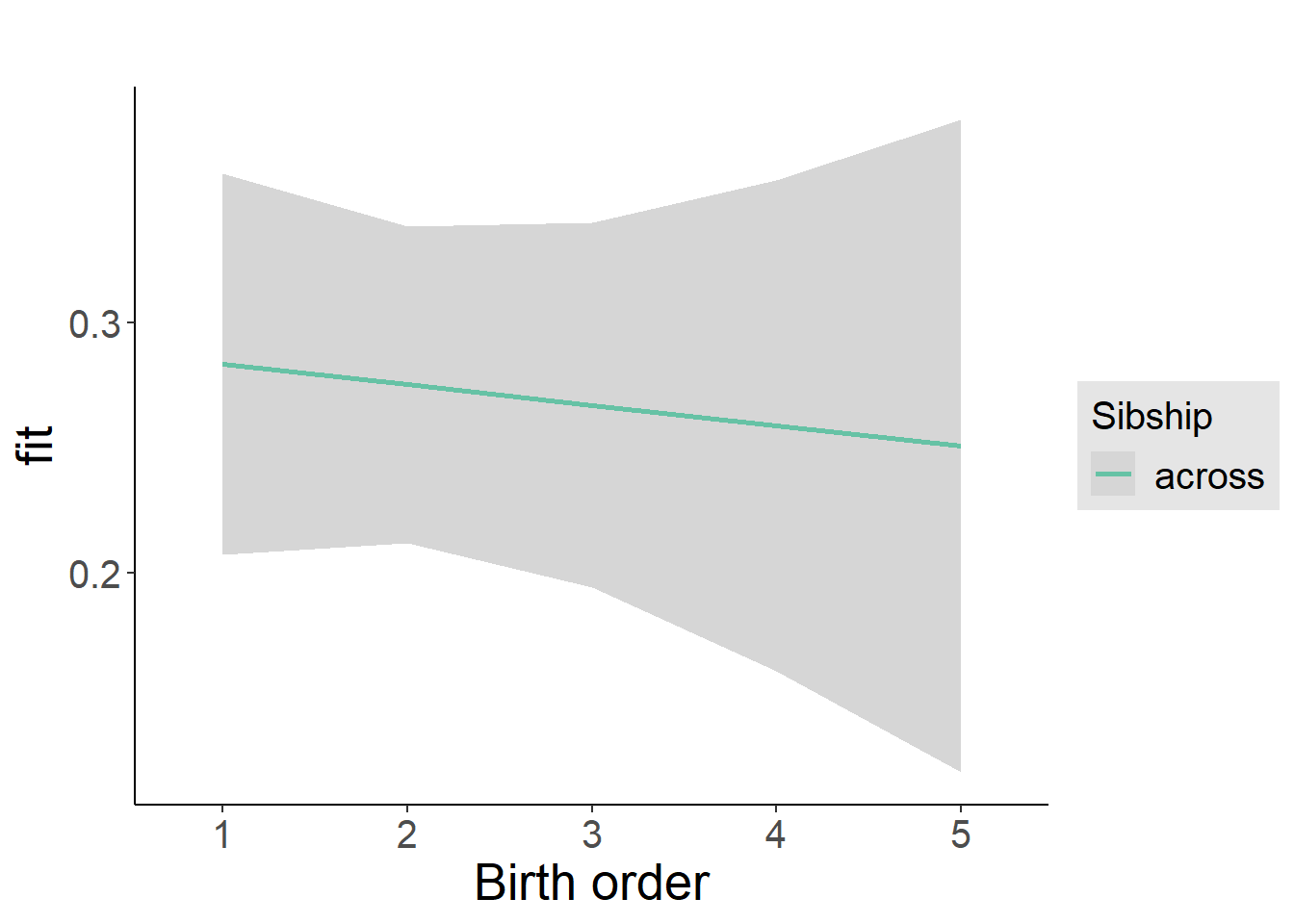
Add Birth Order Factor
Model Summary
m3_birthorder_nonlinear = update(m1_covariates_only, formula = . ~ . + birth_order_nonlinear)
tidy(m3_birthorder_nonlinear, conf.int = T, conf.level = 0.995)| effect | group | term | estimate | std.error | statistic | df | p.value | conf.low | conf.high |
|---|---|---|---|---|---|---|---|---|---|
| fixed | NA | (Intercept) | -1.722 | 0.4979 | -3.458 | 4436 | 0.0005496 | -3.12 | -0.3241 |
| fixed | NA | poly(age, 3, raw = TRUE)1 | 0.204 | 0.05805 | 3.515 | 4439 | 0.0004447 | 0.04108 | 0.367 |
| fixed | NA | poly(age, 3, raw = TRUE)2 | -0.006583 | 0.002139 | -3.077 | 4443 | 0.002101 | -0.01259 | -0.0005785 |
| fixed | NA | poly(age, 3, raw = TRUE)3 | 0.00006572 | 0.00002507 | 2.622 | 4445 | 0.008782 | -0.000004648 | 0.0001361 |
| fixed | NA | male | -0.005921 | 0.0267 | -0.2217 | 4298 | 0.8246 | -0.08088 | 0.06904 |
| fixed | NA | sibling_count3 | 0.009106 | 0.03835 | 0.2375 | 3333 | 0.8123 | -0.09853 | 0.1167 |
| fixed | NA | sibling_count4 | -0.008766 | 0.04375 | -0.2004 | 3098 | 0.8412 | -0.1316 | 0.114 |
| fixed | NA | sibling_count5 | -0.05973 | 0.05332 | -1.12 | 3110 | 0.2627 | -0.2094 | 0.08995 |
| fixed | NA | birth_order_nonlinear2 | 0.02484 | 0.03148 | 0.7891 | 3389 | 0.4301 | -0.06352 | 0.1132 |
| fixed | NA | birth_order_nonlinear3 | -0.0727 | 0.04012 | -1.812 | 3598 | 0.07004 | -0.1853 | 0.03991 |
| fixed | NA | birth_order_nonlinear4 | 0.0009335 | 0.05412 | 0.01725 | 3786 | 0.9862 | -0.151 | 0.1529 |
| fixed | NA | birth_order_nonlinear5 | 0.01743 | 0.08369 | 0.2083 | 3617 | 0.835 | -0.2175 | 0.2524 |
| ran_pars | mother_pidlink | sd__(Intercept) | 0.3834 | NA | NA | NA | NA | NA | NA |
| ran_pars | Residual | sd__Observation | 0.8163 | NA | NA | NA | NA | NA | NA |
Coefficient Plot
plot_birthorder(m3_birthorder_nonlinear, separate = FALSE)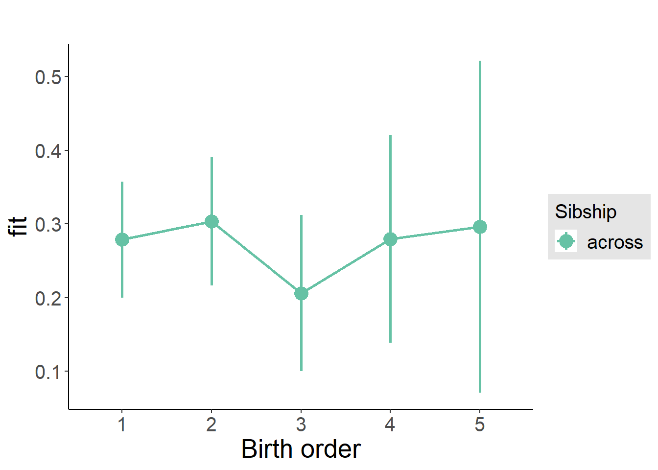
Add Interaction
Model Summary
m4_interaction = update(m3_birthorder_nonlinear, formula = . ~ . - birth_order_nonlinear - sibling_count + count_birth_order)
tidy(m4_interaction, conf.int = T, conf.level = 0.995)| effect | group | term | estimate | std.error | statistic | df | p.value | conf.low | conf.high |
|---|---|---|---|---|---|---|---|---|---|
| fixed | NA | (Intercept) | -1.725 | 0.4981 | -3.463 | 4430 | 0.0005388 | -3.123 | -0.3269 |
| fixed | NA | poly(age, 3, raw = TRUE)1 | 0.2031 | 0.05807 | 3.498 | 4432 | 0.0004726 | 0.04015 | 0.3661 |
| fixed | NA | poly(age, 3, raw = TRUE)2 | -0.00655 | 0.00214 | -3.061 | 4436 | 0.002221 | -0.01256 | -0.000543 |
| fixed | NA | poly(age, 3, raw = TRUE)3 | 0.0000653 | 0.00002508 | 2.604 | 4438 | 0.009257 | -0.000005104 | 0.0001357 |
| fixed | NA | male | -0.007608 | 0.02672 | -0.2847 | 4291 | 0.7759 | -0.08261 | 0.06739 |
| fixed | NA | count_birth_order2/2 | 0.06025 | 0.05431 | 1.109 | 3647 | 0.2674 | -0.0922 | 0.2127 |
| fixed | NA | count_birth_order1/3 | 0.04044 | 0.04845 | 0.8346 | 4417 | 0.404 | -0.09557 | 0.1764 |
| fixed | NA | count_birth_order2/3 | 0.005604 | 0.05278 | 0.1062 | 4439 | 0.9154 | -0.1425 | 0.1537 |
| fixed | NA | count_birth_order3/3 | -0.03423 | 0.05885 | -0.5815 | 4432 | 0.5609 | -0.1994 | 0.131 |
| fixed | NA | count_birth_order1/4 | -0.03384 | 0.05957 | -0.5682 | 4436 | 0.57 | -0.2011 | 0.1334 |
| fixed | NA | count_birth_order2/4 | 0.08197 | 0.06152 | 1.332 | 4436 | 0.1828 | -0.09072 | 0.2547 |
| fixed | NA | count_birth_order3/4 | -0.07529 | 0.06448 | -1.168 | 4412 | 0.243 | -0.2563 | 0.1057 |
| fixed | NA | count_birth_order4/4 | -0.004362 | 0.06717 | -0.06494 | 4404 | 0.9482 | -0.1929 | 0.1842 |
| fixed | NA | count_birth_order1/5 | 0.01059 | 0.08027 | 0.1319 | 4427 | 0.8951 | -0.2147 | 0.2359 |
| fixed | NA | count_birth_order2/5 | -0.0757 | 0.0861 | -0.8793 | 4373 | 0.3793 | -0.3174 | 0.166 |
| fixed | NA | count_birth_order3/5 | -0.1512 | 0.08077 | -1.872 | 4370 | 0.06127 | -0.3779 | 0.07552 |
| fixed | NA | count_birth_order4/5 | -0.03478 | 0.07775 | -0.4474 | 4393 | 0.6546 | -0.253 | 0.1835 |
| fixed | NA | count_birth_order5/5 | -0.03065 | 0.08022 | -0.3821 | 4371 | 0.7024 | -0.2558 | 0.1945 |
| ran_pars | mother_pidlink | sd__(Intercept) | 0.383 | NA | NA | NA | NA | NA | NA |
| ran_pars | Residual | sd__Observation | 0.8165 | NA | NA | NA | NA | NA | NA |
Coefficient Plot
plot_birthorder(m4_interaction)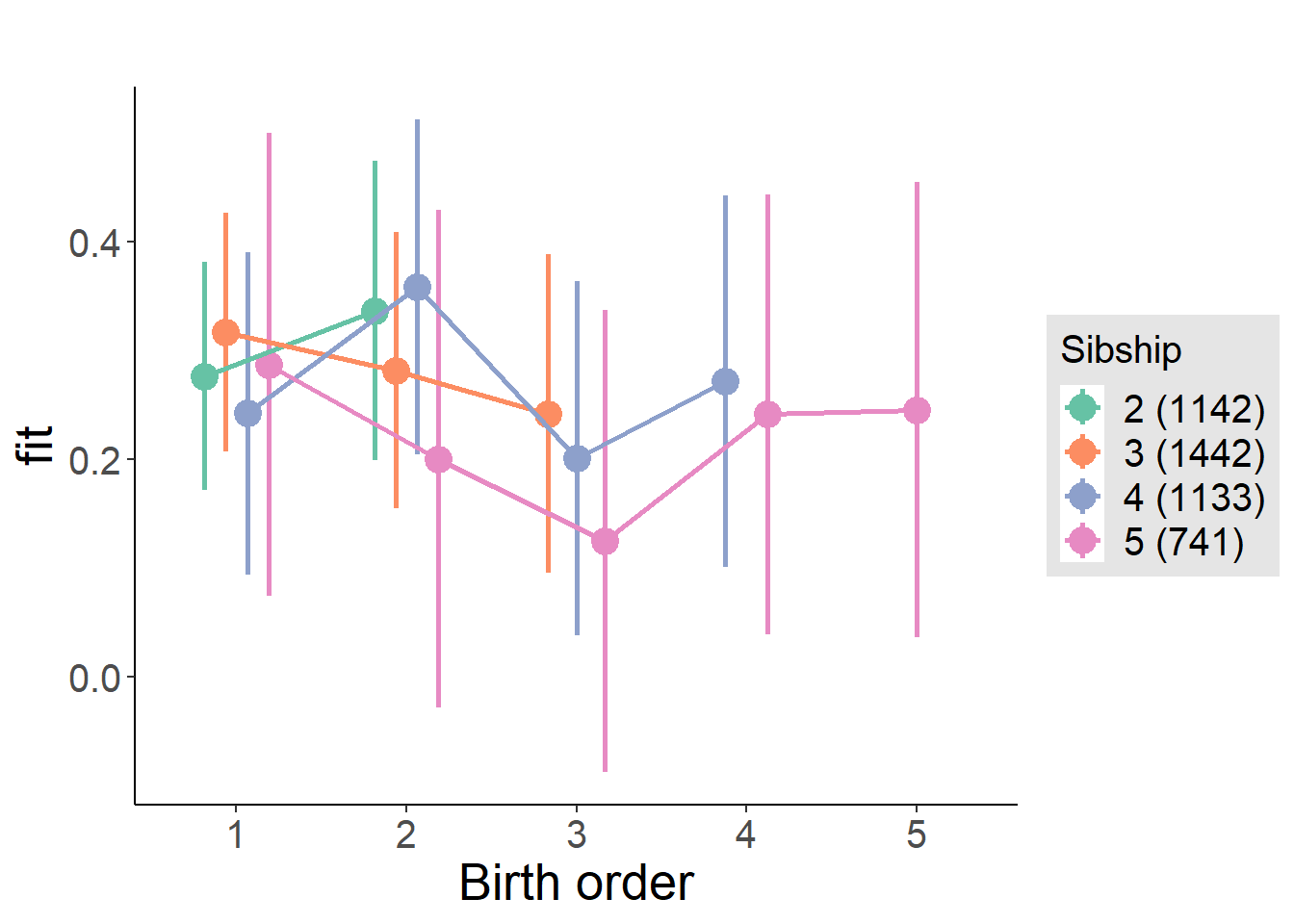
Model Comparison
###### Model 1 - Model 2
anova(m1_covariates_only, m2_birthorder_linear, m3_birthorder_nonlinear, m4_interaction)## refitting model(s) with ML (instead of REML)| Df | AIC | BIC | logLik | deviance | Chisq | Chi Df | Pr(>Chisq) |
|---|---|---|---|---|---|---|---|
| 10 | 11689 | 11753 | -5835 | 11669 | NA | NA | NA |
| 11 | 11691 | 11761 | -5834 | 11669 | 0.3407 | 1 | 0.5594 |
| 14 | 11691 | 11781 | -5832 | 11663 | 5.603 | 3 | 0.1326 |
| 20 | 11698 | 11826 | -5829 | 11658 | 5.166 | 6 | 0.5227 |
Maternal pregnancy order
outcome_preg_m1 <- update(m2_birthorder_linear, data = birthorder %>%
mutate(sibling_count = sibling_count_uterus_preg_factor,
birth_order_nonlinear = birthorder_uterus_preg_factor,
birth_order = birthorder_uterus_preg,
count_birth_order = count_birthorder_uterus_preg
) %>%
filter(sibling_count != "1"))
compare_models_markdown(outcome_preg_m1)Basic Model
Model Summary
m1_covariates_only <- update(m2_birthorder_linear, formula = . ~ . - birth_order)
tidy(m1_covariates_only, conf.int = T, conf.level = 0.995)| effect | group | term | estimate | std.error | statistic | df | p.value | conf.low | conf.high |
|---|---|---|---|---|---|---|---|---|---|
| fixed | NA | (Intercept) | -1.672 | 0.5143 | -3.251 | 4112 | 0.001158 | -3.116 | -0.2285 |
| fixed | NA | poly(age, 3, raw = TRUE)1 | 0.2008 | 0.06007 | 3.343 | 4117 | 0.0008354 | 0.03221 | 0.3694 |
| fixed | NA | poly(age, 3, raw = TRUE)2 | -0.006501 | 0.002214 | -2.936 | 4123 | 0.003344 | -0.01272 | -0.0002855 |
| fixed | NA | poly(age, 3, raw = TRUE)3 | 0.00006511 | 0.00002594 | 2.51 | 4126 | 0.01213 | -0.000007718 | 0.0001379 |
| fixed | NA | male | -0.002898 | 0.02786 | -0.104 | 3986 | 0.9172 | -0.08111 | 0.07532 |
| fixed | NA | sibling_count3 | -0.03883 | 0.04046 | -0.9596 | 3017 | 0.3373 | -0.1524 | 0.07476 |
| fixed | NA | sibling_count4 | -0.01039 | 0.04301 | -0.2416 | 2746 | 0.8091 | -0.1311 | 0.1103 |
| fixed | NA | sibling_count5 | -0.07237 | 0.04605 | -1.572 | 2485 | 0.1162 | -0.2016 | 0.0569 |
| ran_pars | mother_pidlink | sd__(Intercept) | 0.3864 | NA | NA | NA | NA | NA | NA |
| ran_pars | Residual | sd__Observation | 0.82 | NA | NA | NA | NA | NA | NA |
Coefficient Plot
plot(allEffects(m1_covariates_only, confidence.level = 0.995))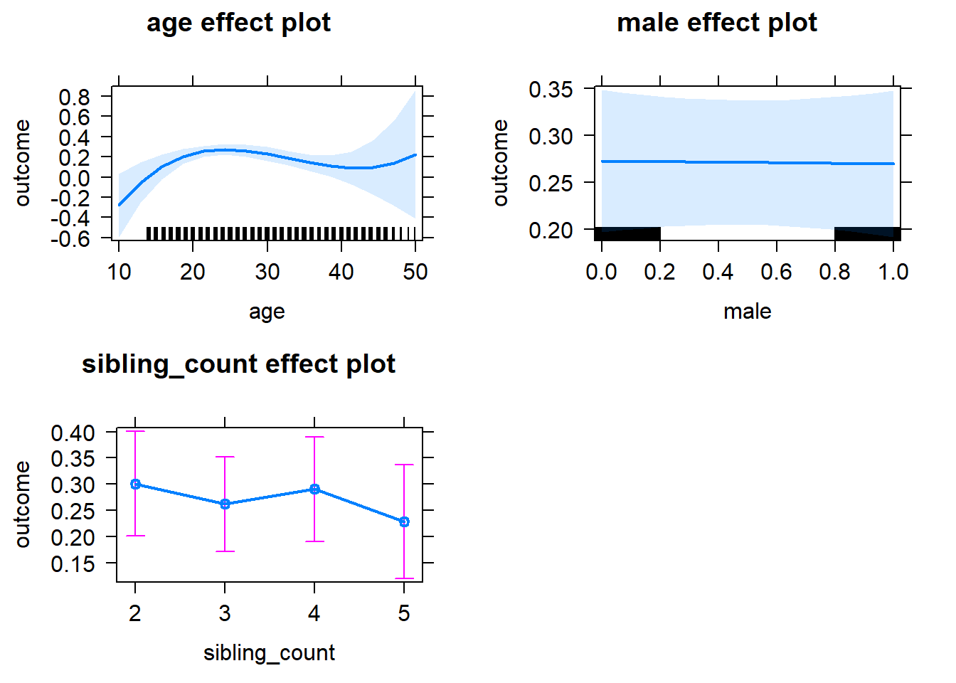
Add Birth Order Linear
Model Summary
tidy(m2_birthorder_linear, conf.int = T, conf.level = 0.995)| effect | group | term | estimate | std.error | statistic | df | p.value | conf.low | conf.high |
|---|---|---|---|---|---|---|---|---|---|
| fixed | NA | (Intercept) | -1.643 | 0.5148 | -3.191 | 4110 | 0.00143 | -3.088 | -0.1975 |
| fixed | NA | birth_order | -0.01829 | 0.01405 | -1.302 | 3793 | 0.1929 | -0.05772 | 0.02114 |
| fixed | NA | poly(age, 3, raw = TRUE)1 | 0.2 | 0.06006 | 3.33 | 4116 | 0.0008748 | 0.03144 | 0.3686 |
| fixed | NA | poly(age, 3, raw = TRUE)2 | -0.006456 | 0.002214 | -2.916 | 4121 | 0.003569 | -0.01267 | -0.0002404 |
| fixed | NA | poly(age, 3, raw = TRUE)3 | 0.00006421 | 0.00002595 | 2.474 | 4124 | 0.01339 | -0.000008632 | 0.0001371 |
| fixed | NA | male | -0.002367 | 0.02786 | -0.08495 | 3983 | 0.9323 | -0.08057 | 0.07584 |
| fixed | NA | sibling_count3 | -0.0303 | 0.041 | -0.739 | 3058 | 0.4599 | -0.1454 | 0.0848 |
| fixed | NA | sibling_count4 | 0.008544 | 0.04542 | 0.1881 | 2912 | 0.8508 | -0.119 | 0.136 |
| fixed | NA | sibling_count5 | -0.04233 | 0.05155 | -0.821 | 2873 | 0.4117 | -0.187 | 0.1024 |
| ran_pars | mother_pidlink | sd__(Intercept) | 0.3883 | NA | NA | NA | NA | NA | NA |
| ran_pars | Residual | sd__Observation | 0.8191 | NA | NA | NA | NA | NA | NA |
Coefficient Plot
plot_birthorder2(m2_birthorder_linear, separate = FALSE)
Add Birth Order Factor
Model Summary
m3_birthorder_nonlinear = update(m1_covariates_only, formula = . ~ . + birth_order_nonlinear)
tidy(m3_birthorder_nonlinear, conf.int = T, conf.level = 0.995)| effect | group | term | estimate | std.error | statistic | df | p.value | conf.low | conf.high |
|---|---|---|---|---|---|---|---|---|---|
| fixed | NA | (Intercept) | -1.648 | 0.5152 | -3.199 | 4114 | 0.001387 | -3.094 | -0.2022 |
| fixed | NA | poly(age, 3, raw = TRUE)1 | 0.1975 | 0.06011 | 3.287 | 4117 | 0.001022 | 0.02883 | 0.3663 |
| fixed | NA | poly(age, 3, raw = TRUE)2 | -0.006367 | 0.002216 | -2.873 | 4121 | 0.004081 | -0.01259 | -0.0001472 |
| fixed | NA | poly(age, 3, raw = TRUE)3 | 0.00006325 | 0.00002596 | 2.436 | 4123 | 0.01489 | -0.000009631 | 0.0001361 |
| fixed | NA | male | -0.001729 | 0.02785 | -0.06206 | 3978 | 0.9505 | -0.07991 | 0.07646 |
| fixed | NA | sibling_count3 | -0.0167 | 0.04155 | -0.4019 | 3160 | 0.6878 | -0.1333 | 0.09994 |
| fixed | NA | sibling_count4 | 0.02424 | 0.04601 | 0.5268 | 3006 | 0.5983 | -0.1049 | 0.1534 |
| fixed | NA | sibling_count5 | -0.04462 | 0.05203 | -0.8576 | 2929 | 0.3912 | -0.1907 | 0.1014 |
| fixed | NA | birth_order_nonlinear2 | 0.006307 | 0.03295 | 0.1914 | 3211 | 0.8482 | -0.08619 | 0.0988 |
| fixed | NA | birth_order_nonlinear3 | -0.0971 | 0.04164 | -2.332 | 3409 | 0.01978 | -0.214 | 0.0198 |
| fixed | NA | birth_order_nonlinear4 | -0.06401 | 0.0554 | -1.155 | 3557 | 0.248 | -0.2195 | 0.0915 |
| fixed | NA | birth_order_nonlinear5 | 0.03111 | 0.08057 | 0.3861 | 3421 | 0.6995 | -0.1951 | 0.2573 |
| ran_pars | mother_pidlink | sd__(Intercept) | 0.3886 | NA | NA | NA | NA | NA | NA |
| ran_pars | Residual | sd__Observation | 0.8186 | NA | NA | NA | NA | NA | NA |
Coefficient Plot
plot_birthorder(m3_birthorder_nonlinear, separate = FALSE)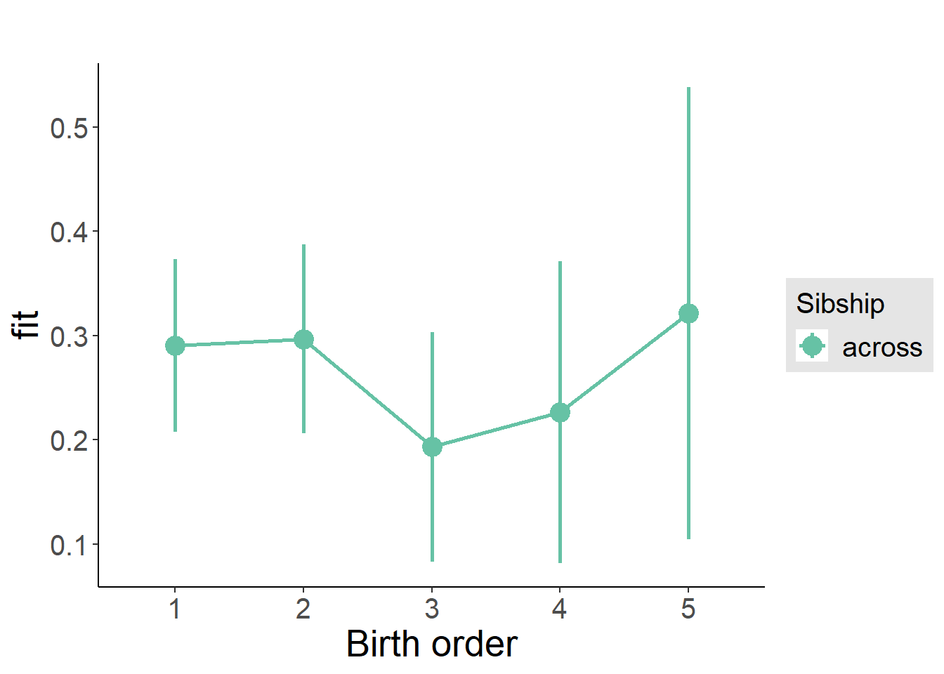
Add Interaction
Model Summary
m4_interaction = update(m3_birthorder_nonlinear, formula = . ~ . - birth_order_nonlinear - sibling_count + count_birth_order)
tidy(m4_interaction, conf.int = T, conf.level = 0.995)| effect | group | term | estimate | std.error | statistic | df | p.value | conf.low | conf.high |
|---|---|---|---|---|---|---|---|---|---|
| fixed | NA | (Intercept) | -1.699 | 0.5152 | -3.297 | 4107 | 0.0009849 | -3.145 | -0.2525 |
| fixed | NA | poly(age, 3, raw = TRUE)1 | 0.2 | 0.06009 | 3.327 | 4110 | 0.0008841 | 0.03127 | 0.3686 |
| fixed | NA | poly(age, 3, raw = TRUE)2 | -0.006461 | 0.002215 | -2.916 | 4114 | 0.003561 | -0.01268 | -0.0002421 |
| fixed | NA | poly(age, 3, raw = TRUE)3 | 0.00006434 | 0.00002597 | 2.478 | 4117 | 0.01326 | -0.000008549 | 0.0001372 |
| fixed | NA | male | -0.003124 | 0.02785 | -0.1122 | 3965 | 0.9107 | -0.08129 | 0.07504 |
| fixed | NA | count_birth_order2/2 | 0.1048 | 0.05963 | 1.758 | 3436 | 0.07879 | -0.06254 | 0.2722 |
| fixed | NA | count_birth_order1/3 | 0.04469 | 0.05273 | 0.8475 | 4099 | 0.3968 | -0.1033 | 0.1927 |
| fixed | NA | count_birth_order2/3 | -0.03942 | 0.05694 | -0.6923 | 4118 | 0.4888 | -0.1992 | 0.1204 |
| fixed | NA | count_birth_order3/3 | -0.04743 | 0.06392 | -0.742 | 4111 | 0.4581 | -0.2269 | 0.132 |
| fixed | NA | count_birth_order1/4 | 0.07906 | 0.06266 | 1.262 | 4115 | 0.2071 | -0.09682 | 0.2549 |
| fixed | NA | count_birth_order2/4 | 0.1188 | 0.06378 | 1.862 | 4118 | 0.06263 | -0.06026 | 0.2978 |
| fixed | NA | count_birth_order3/4 | -0.09997 | 0.06932 | -1.442 | 4088 | 0.1493 | -0.2945 | 0.0946 |
| fixed | NA | count_birth_order4/4 | -0.05328 | 0.07163 | -0.7438 | 4086 | 0.457 | -0.2544 | 0.1478 |
| fixed | NA | count_birth_order1/5 | -0.01956 | 0.07394 | -0.2645 | 4118 | 0.7914 | -0.2271 | 0.188 |
| fixed | NA | count_birth_order2/5 | -0.07445 | 0.07938 | -0.9379 | 4079 | 0.3483 | -0.2973 | 0.1484 |
| fixed | NA | count_birth_order3/5 | -0.08677 | 0.07702 | -1.127 | 4070 | 0.26 | -0.303 | 0.1294 |
| fixed | NA | count_birth_order4/5 | -0.01681 | 0.07992 | -0.2104 | 4043 | 0.8334 | -0.2412 | 0.2075 |
| fixed | NA | count_birth_order5/5 | 0.02023 | 0.0795 | 0.2545 | 4046 | 0.7991 | -0.2029 | 0.2434 |
| ran_pars | mother_pidlink | sd__(Intercept) | 0.3926 | NA | NA | NA | NA | NA | NA |
| ran_pars | Residual | sd__Observation | 0.8164 | NA | NA | NA | NA | NA | NA |
Coefficient Plot
plot_birthorder(m4_interaction)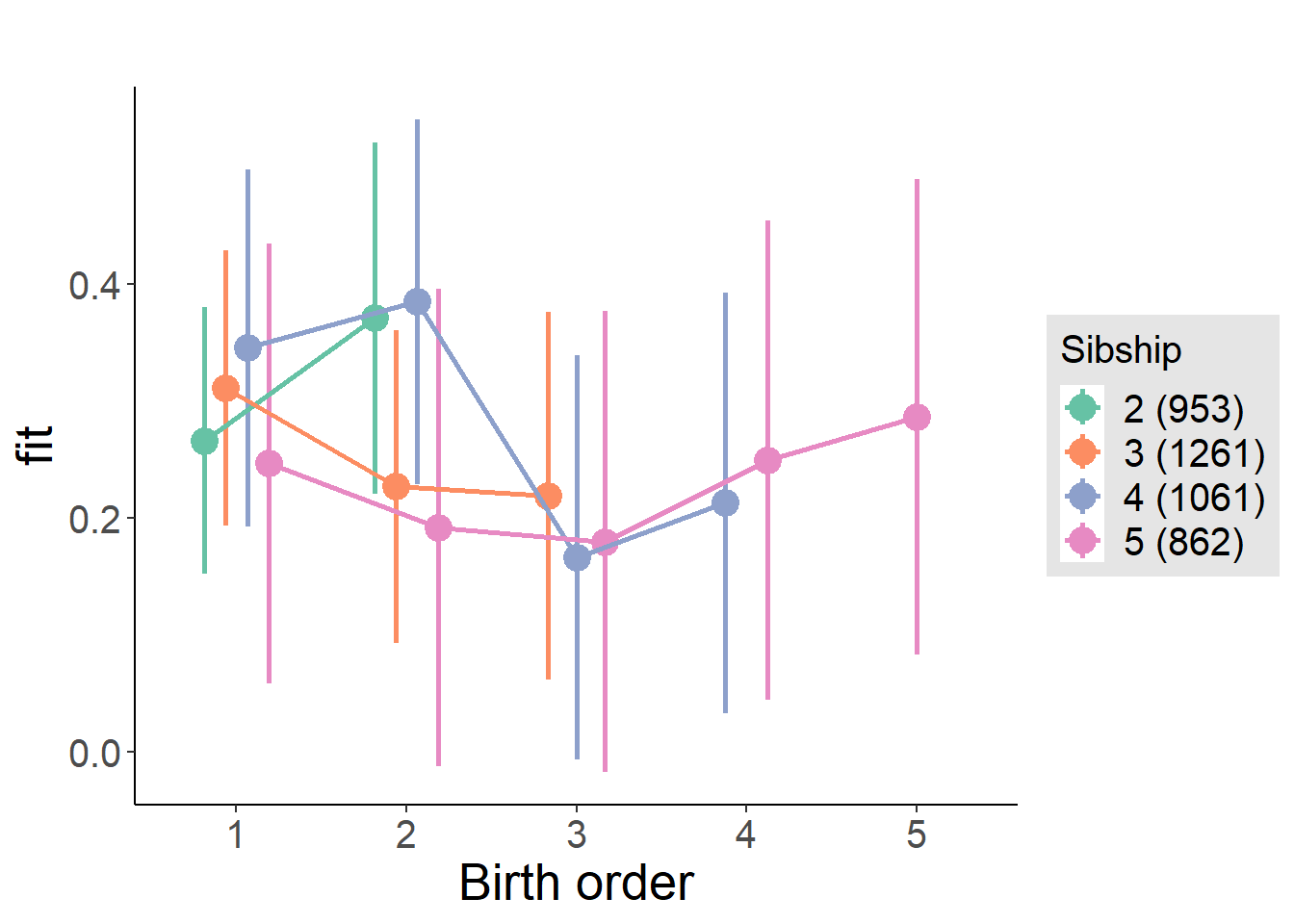
Model Comparison
###### Model 1 - Model 2
anova(m1_covariates_only, m2_birthorder_linear, m3_birthorder_nonlinear, m4_interaction)## refitting model(s) with ML (instead of REML)| Df | AIC | BIC | logLik | deviance | Chisq | Chi Df | Pr(>Chisq) |
|---|---|---|---|---|---|---|---|
| 10 | 10890 | 10953 | -5435 | 10870 | NA | NA | NA |
| 11 | 10890 | 10960 | -5434 | 10868 | 1.69 | 1 | 0.1937 |
| 14 | 10890 | 10978 | -5431 | 10862 | 6.354 | 3 | 0.09561 |
| 20 | 10891 | 11018 | -5426 | 10851 | 10.89 | 6 | 0.09181 |
Parental full sibling order
outcome_parental_m1 <- update(m2_birthorder_linear, data = birthorder %>%
mutate(sibling_count = sibling_count_genes_factor,
birth_order_nonlinear = birthorder_genes_factor,
birth_order = birthorder_genes,
count_birth_order = count_birthorder_genes
) %>%
filter(sibling_count != "1"))
compare_models_markdown(outcome_parental_m1)Basic Model
Model Summary
m1_covariates_only <- update(m2_birthorder_linear, formula = . ~ . - birth_order)
tidy(m1_covariates_only, conf.int = T, conf.level = 0.995)| effect | group | term | estimate | std.error | statistic | df | p.value | conf.low | conf.high |
|---|---|---|---|---|---|---|---|---|---|
| fixed | NA | (Intercept) | -1.806 | 0.4996 | -3.615 | 4423 | 0.0003036 | -3.209 | -0.4037 |
| fixed | NA | poly(age, 3, raw = TRUE)1 | 0.212 | 0.05838 | 3.631 | 4428 | 0.000286 | 0.04808 | 0.3758 |
| fixed | NA | poly(age, 3, raw = TRUE)2 | -0.006831 | 0.002155 | -3.171 | 4433 | 0.001532 | -0.01288 | -0.0007832 |
| fixed | NA | poly(age, 3, raw = TRUE)3 | 0.00006775 | 0.00002529 | 2.679 | 4436 | 0.007417 | -0.000003245 | 0.0001387 |
| fixed | NA | male | -0.003468 | 0.02666 | -0.1301 | 4304 | 0.8965 | -0.0783 | 0.07137 |
| fixed | NA | sibling_count3 | 0.02394 | 0.03657 | 0.6547 | 3158 | 0.5127 | -0.07872 | 0.1266 |
| fixed | NA | sibling_count4 | -0.01511 | 0.03993 | -0.3784 | 2796 | 0.7051 | -0.1272 | 0.09697 |
| fixed | NA | sibling_count5 | -0.02829 | 0.0471 | -0.6006 | 2438 | 0.5481 | -0.1605 | 0.1039 |
| ran_pars | mother_pidlink | sd__(Intercept) | 0.3744 | NA | NA | NA | NA | NA | NA |
| ran_pars | Residual | sd__Observation | 0.8164 | NA | NA | NA | NA | NA | NA |
Coefficient Plot
plot(allEffects(m1_covariates_only, confidence.level = 0.995))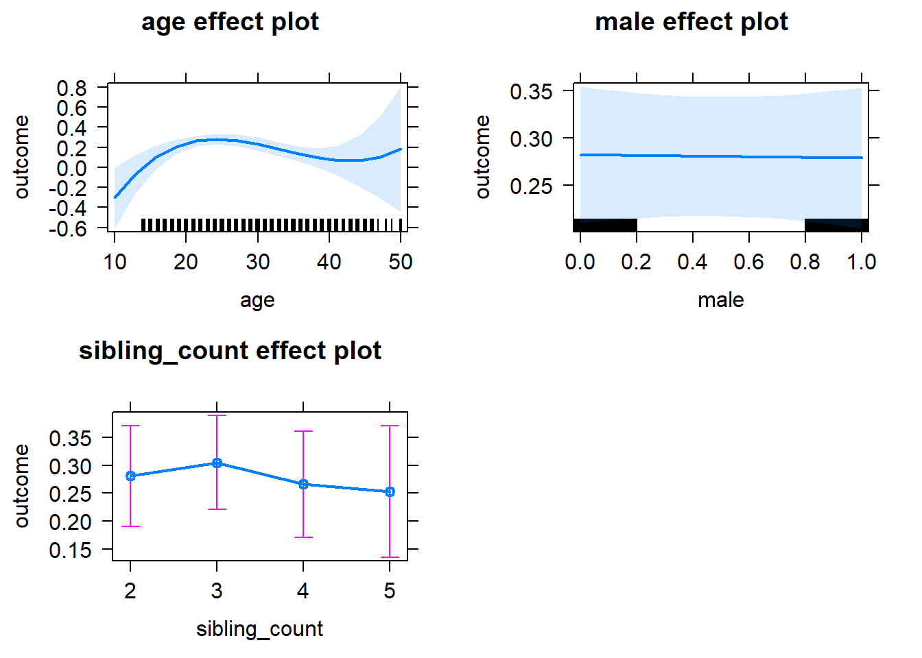
Add Birth Order Linear
Model Summary
tidy(m2_birthorder_linear, conf.int = T, conf.level = 0.995)| effect | group | term | estimate | std.error | statistic | df | p.value | conf.low | conf.high |
|---|---|---|---|---|---|---|---|---|---|
| fixed | NA | (Intercept) | -1.784 | 0.5002 | -3.567 | 4422 | 0.0003648 | -3.188 | -0.3802 |
| fixed | NA | birth_order | -0.01327 | 0.01407 | -0.9433 | 3979 | 0.3456 | -0.05276 | 0.02622 |
| fixed | NA | poly(age, 3, raw = TRUE)1 | 0.2113 | 0.05839 | 3.619 | 4427 | 0.0002989 | 0.04741 | 0.3752 |
| fixed | NA | poly(age, 3, raw = TRUE)2 | -0.006794 | 0.002155 | -3.153 | 4431 | 0.001628 | -0.01284 | -0.0007451 |
| fixed | NA | poly(age, 3, raw = TRUE)3 | 0.00006705 | 0.0000253 | 2.65 | 4434 | 0.008086 | -0.000003982 | 0.0001381 |
| fixed | NA | male | -0.00305 | 0.02666 | -0.1144 | 4300 | 0.9089 | -0.07789 | 0.07179 |
| fixed | NA | sibling_count3 | 0.0301 | 0.03716 | 0.8101 | 3214 | 0.418 | -0.07421 | 0.1344 |
| fixed | NA | sibling_count4 | -0.0009211 | 0.04269 | -0.02157 | 3032 | 0.9828 | -0.1208 | 0.1189 |
| fixed | NA | sibling_count5 | -0.005691 | 0.05287 | -0.1076 | 2892 | 0.9143 | -0.1541 | 0.1427 |
| ran_pars | mother_pidlink | sd__(Intercept) | 0.376 | NA | NA | NA | NA | NA | NA |
| ran_pars | Residual | sd__Observation | 0.8158 | NA | NA | NA | NA | NA | NA |
Coefficient Plot
plot_birthorder2(m2_birthorder_linear, separate = FALSE)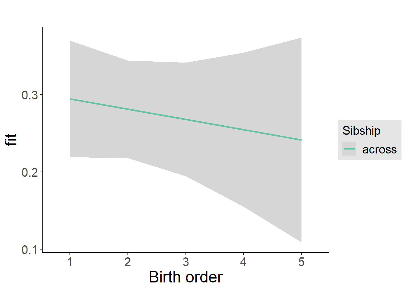
Add Birth Order Factor
Model Summary
m3_birthorder_nonlinear = update(m1_covariates_only, formula = . ~ . + birth_order_nonlinear)
tidy(m3_birthorder_nonlinear, conf.int = T, conf.level = 0.995)| effect | group | term | estimate | std.error | statistic | df | p.value | conf.low | conf.high |
|---|---|---|---|---|---|---|---|---|---|
| fixed | NA | (Intercept) | -1.787 | 0.5006 | -3.569 | 4424 | 0.0003622 | -3.192 | -0.3814 |
| fixed | NA | poly(age, 3, raw = TRUE)1 | 0.2092 | 0.05844 | 3.58 | 4427 | 0.0003477 | 0.04516 | 0.3733 |
| fixed | NA | poly(age, 3, raw = TRUE)2 | -0.006723 | 0.002157 | -3.117 | 4430 | 0.00184 | -0.01278 | -0.0006681 |
| fixed | NA | poly(age, 3, raw = TRUE)3 | 0.00006633 | 0.00002532 | 2.619 | 4432 | 0.008841 | -0.000004754 | 0.0001374 |
| fixed | NA | male | -0.003809 | 0.02666 | -0.1429 | 4293 | 0.8864 | -0.07864 | 0.07102 |
| fixed | NA | sibling_count3 | 0.04375 | 0.03773 | 1.16 | 3336 | 0.2463 | -0.06216 | 0.1497 |
| fixed | NA | sibling_count4 | 0.004315 | 0.04332 | 0.09961 | 3136 | 0.9207 | -0.1173 | 0.1259 |
| fixed | NA | sibling_count5 | -0.006141 | 0.05392 | -0.1139 | 2999 | 0.9093 | -0.1575 | 0.1452 |
| fixed | NA | birth_order_nonlinear2 | 0.01023 | 0.0312 | 0.3278 | 3393 | 0.7431 | -0.07736 | 0.09782 |
| fixed | NA | birth_order_nonlinear3 | -0.08294 | 0.03988 | -2.08 | 3581 | 0.03761 | -0.1949 | 0.029 |
| fixed | NA | birth_order_nonlinear4 | 0.006899 | 0.05504 | 0.1253 | 3766 | 0.9003 | -0.1476 | 0.1614 |
| fixed | NA | birth_order_nonlinear5 | -0.02859 | 0.08942 | -0.3197 | 3693 | 0.7492 | -0.2796 | 0.2224 |
| ran_pars | mother_pidlink | sd__(Intercept) | 0.3773 | NA | NA | NA | NA | NA | NA |
| ran_pars | Residual | sd__Observation | 0.815 | NA | NA | NA | NA | NA | NA |
Coefficient Plot
plot_birthorder(m3_birthorder_nonlinear, separate = FALSE)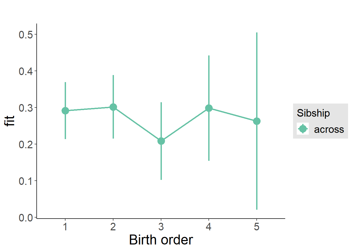
Add Interaction
Model Summary
m4_interaction = update(m3_birthorder_nonlinear, formula = . ~ . - birth_order_nonlinear - sibling_count + count_birth_order)
tidy(m4_interaction, conf.int = T, conf.level = 0.995)| effect | group | term | estimate | std.error | statistic | df | p.value | conf.low | conf.high |
|---|---|---|---|---|---|---|---|---|---|
| fixed | NA | (Intercept) | -1.789 | 0.5009 | -3.571 | 4418 | 0.000359 | -3.195 | -0.3828 |
| fixed | NA | poly(age, 3, raw = TRUE)1 | 0.2077 | 0.05847 | 3.552 | 4421 | 0.0003864 | 0.04356 | 0.3718 |
| fixed | NA | poly(age, 3, raw = TRUE)2 | -0.006655 | 0.002158 | -3.084 | 4424 | 0.002056 | -0.01271 | -0.0005975 |
| fixed | NA | poly(age, 3, raw = TRUE)3 | 0.00006538 | 0.00002534 | 2.58 | 4426 | 0.009902 | -0.000005744 | 0.0001365 |
| fixed | NA | male | -0.004814 | 0.02667 | -0.1805 | 4286 | 0.8568 | -0.07968 | 0.07006 |
| fixed | NA | count_birth_order2/2 | 0.05052 | 0.05269 | 0.9587 | 3606 | 0.3378 | -0.09739 | 0.1984 |
| fixed | NA | count_birth_order1/3 | 0.06193 | 0.04767 | 1.299 | 4404 | 0.194 | -0.07189 | 0.1958 |
| fixed | NA | count_birth_order2/3 | 0.03904 | 0.05254 | 0.7431 | 4427 | 0.4575 | -0.1084 | 0.1865 |
| fixed | NA | count_birth_order3/3 | 0.003967 | 0.05765 | 0.06881 | 4417 | 0.9451 | -0.1579 | 0.1658 |
| fixed | NA | count_birth_order1/4 | 0.01146 | 0.0596 | 0.1923 | 4426 | 0.8475 | -0.1558 | 0.1788 |
| fixed | NA | count_birth_order2/4 | 0.05606 | 0.06117 | 0.9165 | 4420 | 0.3595 | -0.1156 | 0.2278 |
| fixed | NA | count_birth_order3/4 | -0.07676 | 0.06355 | -1.208 | 4396 | 0.2272 | -0.2552 | 0.1016 |
| fixed | NA | count_birth_order4/4 | 0.01228 | 0.06721 | 0.1827 | 4382 | 0.8551 | -0.1764 | 0.2009 |
| fixed | NA | count_birth_order1/5 | 0.07351 | 0.07983 | 0.9209 | 4421 | 0.3572 | -0.1506 | 0.2976 |
| fixed | NA | count_birth_order2/5 | -0.03273 | 0.08845 | -0.37 | 4355 | 0.7114 | -0.281 | 0.2155 |
| fixed | NA | count_birth_order3/5 | -0.1296 | 0.08443 | -1.535 | 4351 | 0.1247 | -0.3667 | 0.1074 |
| fixed | NA | count_birth_order4/5 | 0.03266 | 0.08106 | 0.4029 | 4375 | 0.687 | -0.1949 | 0.2602 |
| fixed | NA | count_birth_order5/5 | -0.02134 | 0.08554 | -0.2495 | 4354 | 0.803 | -0.2615 | 0.2188 |
| ran_pars | mother_pidlink | sd__(Intercept) | 0.3771 | NA | NA | NA | NA | NA | NA |
| ran_pars | Residual | sd__Observation | 0.8153 | NA | NA | NA | NA | NA | NA |
Coefficient Plot
plot_birthorder(m4_interaction)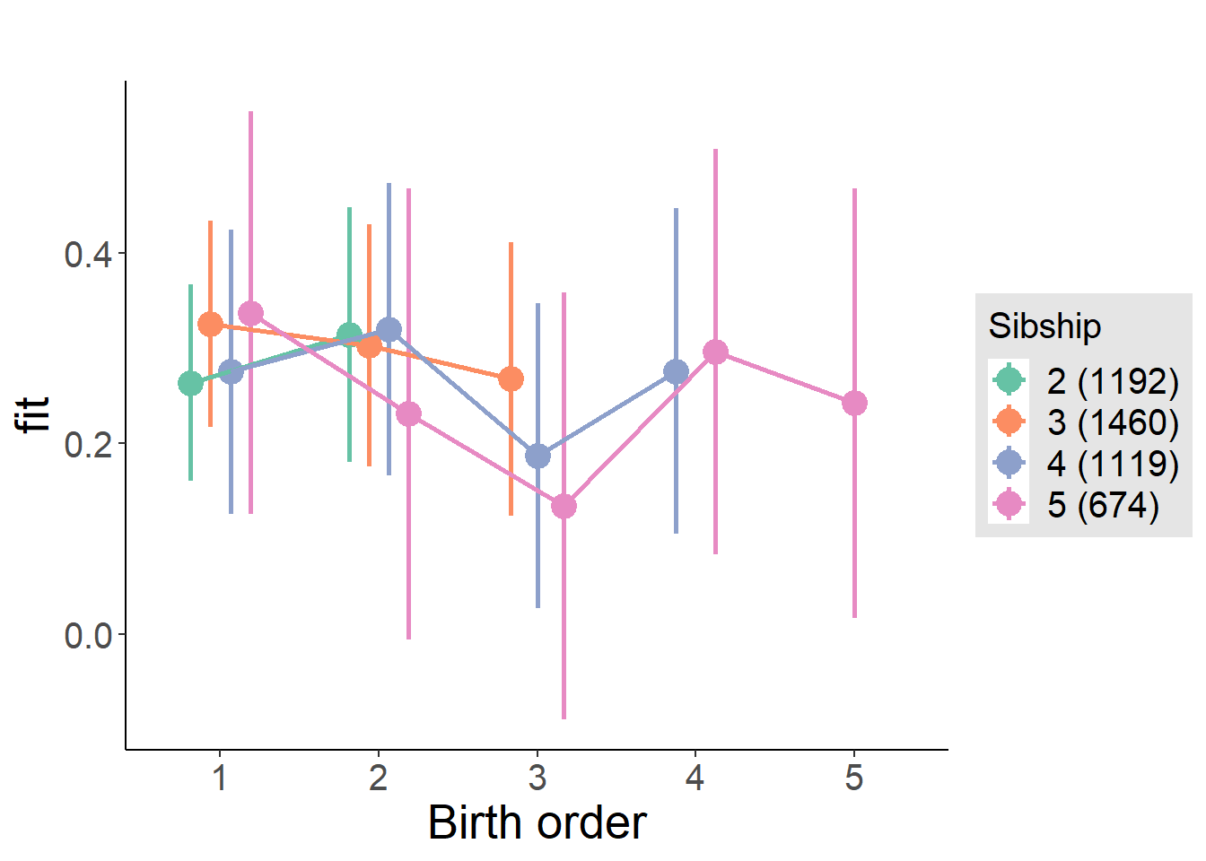
Model Comparison
###### Model 1 - Model 2
anova(m1_covariates_only, m2_birthorder_linear, m3_birthorder_nonlinear, m4_interaction)## refitting model(s) with ML (instead of REML)| Df | AIC | BIC | logLik | deviance | Chisq | Chi Df | Pr(>Chisq) |
|---|---|---|---|---|---|---|---|
| 10 | 11621 | 11685 | -5800 | 11601 | NA | NA | NA |
| 11 | 11622 | 11692 | -5800 | 11600 | 0.884 | 1 | 0.3471 |
| 14 | 11623 | 11712 | -5797 | 11595 | 5.114 | 3 | 0.1636 |
| 20 | 11631 | 11759 | -5795 | 11591 | 3.846 | 6 | 0.6974 |
Compare birth order specifications
library(coefplot)
multiplot(outcome_naive_m1, outcome_preg_m1, outcome_uterus_m1, outcome_parental_m1, dodgeHeight = 0.6,
intercept = FALSE)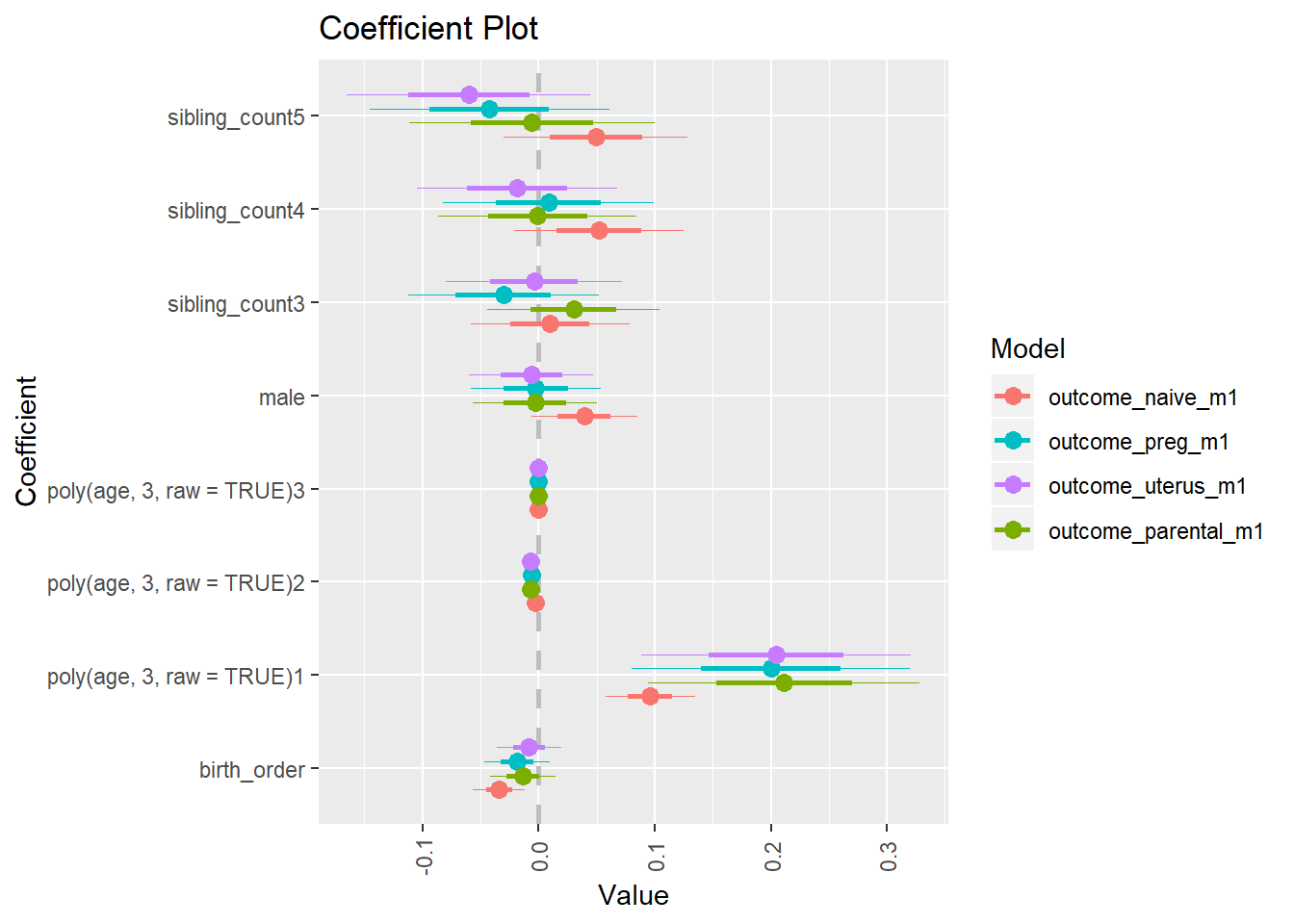
Immediate word recall
birthorder <- birthorder %>% mutate(outcome = words_immediate)
model = lmer(outcome ~ birth_order + poly(age, 3, raw = TRUE) + male + sibling_count + (1 | mother_pidlink),
data = birthorder)
compare_birthorder_specs(model)Naive birth order
outcome_naive_m1 <- update(m2_birthorder_linear, data = birthorder %>%
mutate(sibling_count = sibling_count_naive_factor,
birth_order_nonlinear = birthorder_naive_factor,
birth_order = birthorder_naive,
count_birth_order = count_birthorder_naive) %>%
filter(sibling_count != "1"))
compare_models_markdown(outcome_naive_m1)Basic Model
Model Summary
m1_covariates_only <- update(m2_birthorder_linear, formula = . ~ . - birth_order)
tidy(m1_covariates_only, conf.int = T, conf.level = 0.995)| effect | group | term | estimate | std.error | statistic | df | p.value | conf.low | conf.high |
|---|---|---|---|---|---|---|---|---|---|
| fixed | NA | (Intercept) | 0.04395 | 0.1917 | 0.2292 | 6960 | 0.8187 | -0.4942 | 0.5821 |
| fixed | NA | poly(age, 3, raw = TRUE)1 | 0.04144 | 0.01846 | 2.244 | 6864 | 0.02483 | -0.01039 | 0.09326 |
| fixed | NA | poly(age, 3, raw = TRUE)2 | -0.001579 | 0.0005406 | -2.92 | 6729 | 0.003513 | -0.003096 | -0.000061 |
| fixed | NA | poly(age, 3, raw = TRUE)3 | 0.00001075 | 0.000004915 | 2.187 | 6610 | 0.02874 | -0.000003045 | 0.00002455 |
| fixed | NA | male | -0.08657 | 0.0219 | -3.953 | 6853 | 0.00007805 | -0.148 | -0.02509 |
| fixed | NA | sibling_count3 | 0.02118 | 0.03276 | 0.6466 | 4982 | 0.5179 | -0.07077 | 0.1131 |
| fixed | NA | sibling_count4 | 0.01727 | 0.03395 | 0.5087 | 4558 | 0.611 | -0.07803 | 0.1126 |
| fixed | NA | sibling_count5 | -0.01697 | 0.03553 | -0.4778 | 4111 | 0.6328 | -0.1167 | 0.08275 |
| ran_pars | mother_pidlink | sd__(Intercept) | 0.4299 | NA | NA | NA | NA | NA | NA |
| ran_pars | Residual | sd__Observation | 0.8404 | NA | NA | NA | NA | NA | NA |
Coefficient Plot
plot(allEffects(m1_covariates_only, confidence.level = 0.995))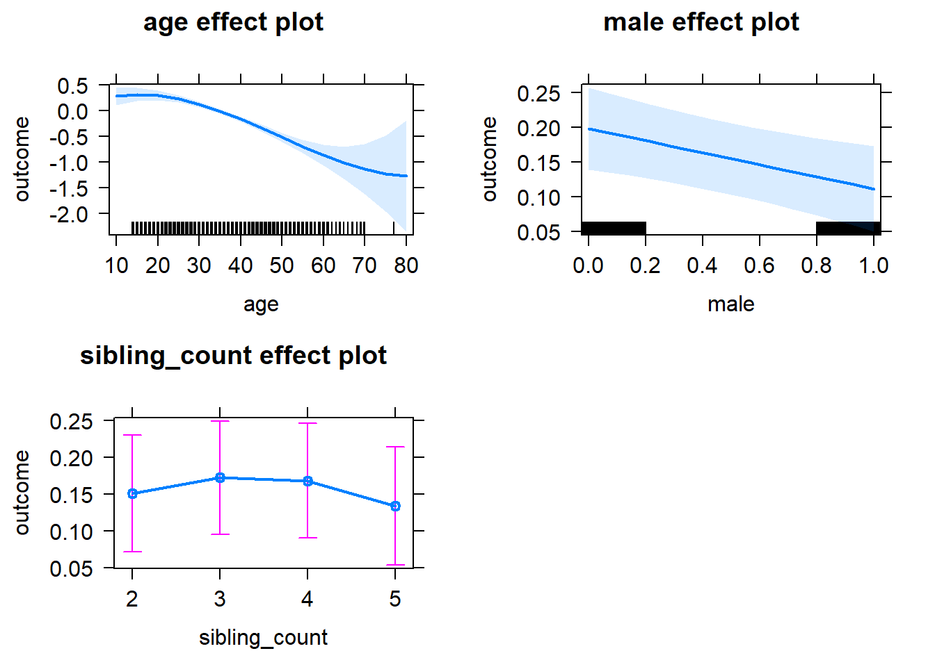
Add Birth Order Linear
Model Summary
tidy(m2_birthorder_linear, conf.int = T, conf.level = 0.995)| effect | group | term | estimate | std.error | statistic | df | p.value | conf.low | conf.high |
|---|---|---|---|---|---|---|---|---|---|
| fixed | NA | (Intercept) | 0.04735 | 0.1918 | 0.2469 | 6947 | 0.805 | -0.4911 | 0.5858 |
| fixed | NA | birth_order | -0.006297 | 0.01078 | -0.5841 | 5827 | 0.5592 | -0.03656 | 0.02397 |
| fixed | NA | poly(age, 3, raw = TRUE)1 | 0.04201 | 0.01849 | 2.272 | 6882 | 0.02311 | -0.009889 | 0.0939 |
| fixed | NA | poly(age, 3, raw = TRUE)2 | -0.001594 | 0.0005413 | -2.945 | 6739 | 0.003244 | -0.003113 | -0.0000745 |
| fixed | NA | poly(age, 3, raw = TRUE)3 | 0.00001085 | 0.000004918 | 2.206 | 6616 | 0.02739 | -0.000002954 | 0.00002466 |
| fixed | NA | male | -0.08641 | 0.0219 | -3.945 | 6851 | 0.00008066 | -0.1479 | -0.02492 |
| fixed | NA | sibling_count3 | 0.02332 | 0.03296 | 0.7075 | 5096 | 0.4793 | -0.06921 | 0.1159 |
| fixed | NA | sibling_count4 | 0.02237 | 0.03505 | 0.6381 | 5040 | 0.5234 | -0.07603 | 0.1208 |
| fixed | NA | sibling_count5 | -0.00868 | 0.03826 | -0.2269 | 5080 | 0.8205 | -0.1161 | 0.09871 |
| ran_pars | mother_pidlink | sd__(Intercept) | 0.4299 | NA | NA | NA | NA | NA | NA |
| ran_pars | Residual | sd__Observation | 0.8404 | NA | NA | NA | NA | NA | NA |
Coefficient Plot
plot_birthorder2(m2_birthorder_linear, separate = FALSE)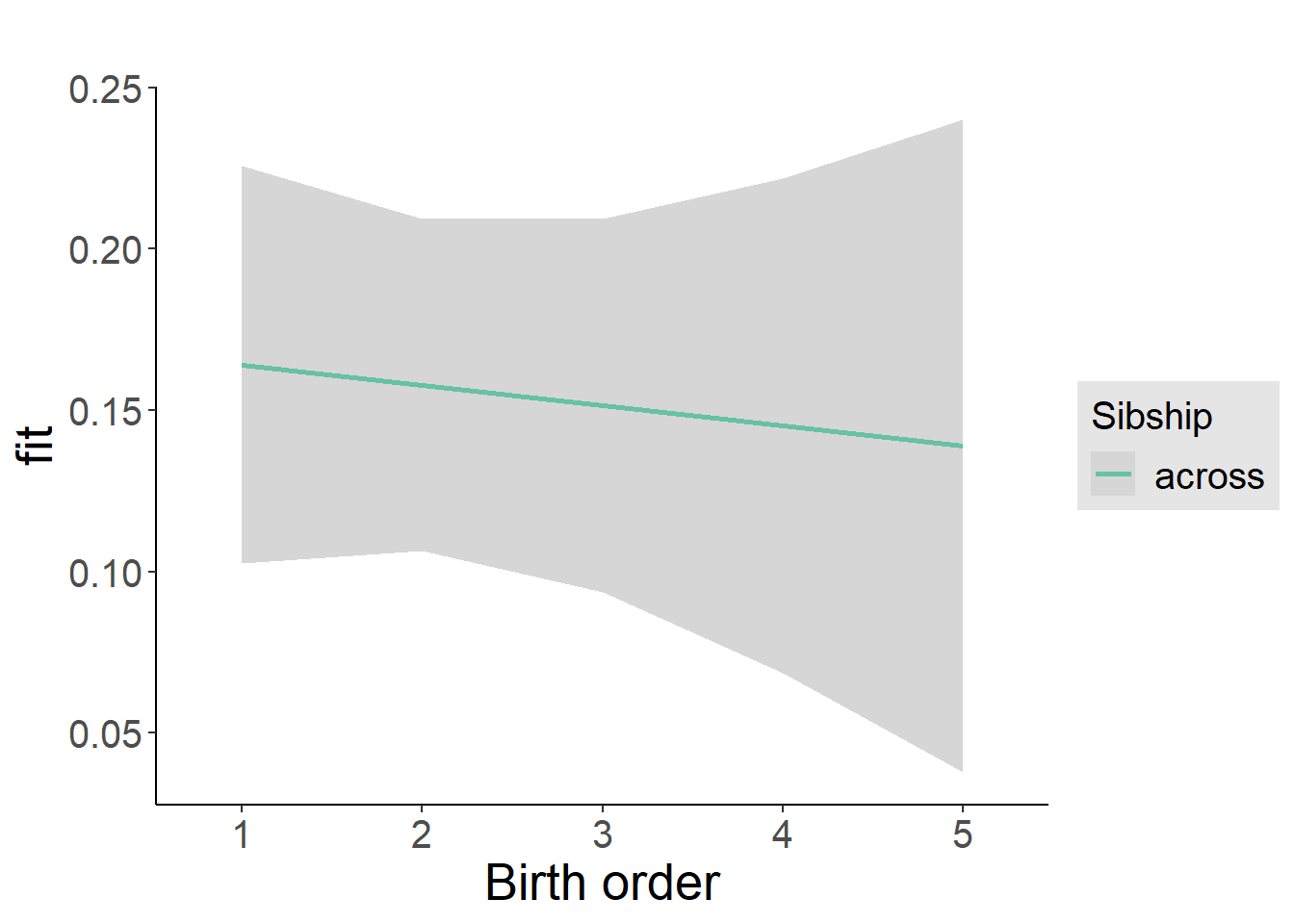
Add Birth Order Factor
Model Summary
m3_birthorder_nonlinear = update(m1_covariates_only, formula = . ~ . + birth_order_nonlinear)
tidy(m3_birthorder_nonlinear, conf.int = T, conf.level = 0.995)| effect | group | term | estimate | std.error | statistic | df | p.value | conf.low | conf.high |
|---|---|---|---|---|---|---|---|---|---|
| fixed | NA | (Intercept) | 0.0379 | 0.1923 | 0.1971 | 6960 | 0.8437 | -0.5018 | 0.5776 |
| fixed | NA | poly(age, 3, raw = TRUE)1 | 0.0421 | 0.0185 | 2.276 | 6867 | 0.0229 | -0.009833 | 0.09404 |
| fixed | NA | poly(age, 3, raw = TRUE)2 | -0.001596 | 0.0005419 | -2.945 | 6714 | 0.003245 | -0.003117 | -0.00007453 |
| fixed | NA | poly(age, 3, raw = TRUE)3 | 0.00001086 | 0.000004927 | 2.204 | 6577 | 0.02754 | -0.00000297 | 0.00002469 |
| fixed | NA | male | -0.08641 | 0.02191 | -3.944 | 6849 | 0.00008098 | -0.1479 | -0.02491 |
| fixed | NA | sibling_count3 | 0.02687 | 0.03341 | 0.8044 | 5287 | 0.4212 | -0.0669 | 0.1206 |
| fixed | NA | sibling_count4 | 0.02511 | 0.03554 | 0.7064 | 5249 | 0.4799 | -0.07466 | 0.1249 |
| fixed | NA | sibling_count5 | -0.007966 | 0.03855 | -0.2066 | 5227 | 0.8363 | -0.1162 | 0.1002 |
| fixed | NA | birth_order_nonlinear2 | -0.001198 | 0.02559 | -0.04681 | 5785 | 0.9627 | -0.07303 | 0.07063 |
| fixed | NA | birth_order_nonlinear3 | -0.02758 | 0.03281 | -0.8407 | 5610 | 0.4006 | -0.1197 | 0.06452 |
| fixed | NA | birth_order_nonlinear4 | -0.01404 | 0.04285 | -0.3276 | 5551 | 0.7432 | -0.1343 | 0.1063 |
| fixed | NA | birth_order_nonlinear5 | -0.01168 | 0.06223 | -0.1876 | 5345 | 0.8512 | -0.1864 | 0.163 |
| ran_pars | mother_pidlink | sd__(Intercept) | 0.4295 | NA | NA | NA | NA | NA | NA |
| ran_pars | Residual | sd__Observation | 0.8408 | NA | NA | NA | NA | NA | NA |
Coefficient Plot
plot_birthorder(m3_birthorder_nonlinear, separate = FALSE)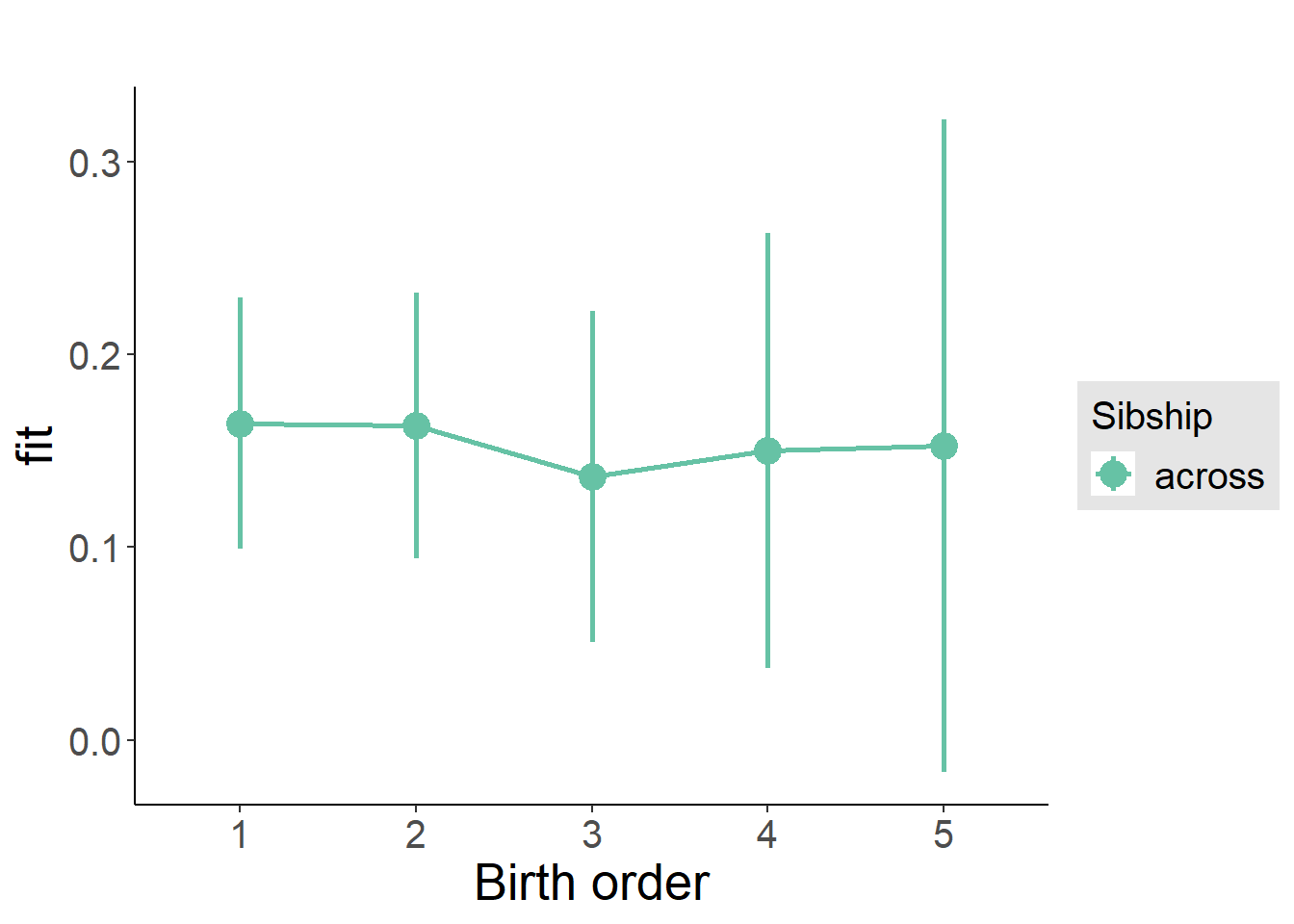
Add Interaction
Model Summary
m4_interaction = update(m3_birthorder_nonlinear, formula = . ~ . - birth_order_nonlinear - sibling_count + count_birth_order)
tidy(m4_interaction, conf.int = T, conf.level = 0.995)| effect | group | term | estimate | std.error | statistic | df | p.value | conf.low | conf.high |
|---|---|---|---|---|---|---|---|---|---|
| fixed | NA | (Intercept) | 0.03058 | 0.1927 | 0.1587 | 6959 | 0.8739 | -0.5102 | 0.5714 |
| fixed | NA | poly(age, 3, raw = TRUE)1 | 0.04236 | 0.0185 | 2.289 | 6862 | 0.02211 | -0.009586 | 0.0943 |
| fixed | NA | poly(age, 3, raw = TRUE)2 | -0.001606 | 0.000542 | -2.964 | 6705 | 0.003052 | -0.003128 | -0.00008481 |
| fixed | NA | poly(age, 3, raw = TRUE)3 | 0.00001098 | 0.000004928 | 2.227 | 6564 | 0.02595 | -0.000002856 | 0.00002481 |
| fixed | NA | male | -0.08653 | 0.02192 | -3.948 | 6842 | 0.00007951 | -0.1481 | -0.02501 |
| fixed | NA | count_birth_order2/2 | 0.0149 | 0.04371 | 0.3408 | 5856 | 0.7332 | -0.1078 | 0.1376 |
| fixed | NA | count_birth_order1/3 | 0.03031 | 0.0424 | 0.7148 | 7068 | 0.4748 | -0.08872 | 0.1493 |
| fixed | NA | count_birth_order2/3 | 0.0312 | 0.04732 | 0.6592 | 7127 | 0.5098 | -0.1016 | 0.164 |
| fixed | NA | count_birth_order3/3 | 0.01083 | 0.05295 | 0.2045 | 7136 | 0.8379 | -0.1378 | 0.1595 |
| fixed | NA | count_birth_order1/4 | 0.003951 | 0.04836 | 0.0817 | 7127 | 0.9349 | -0.1318 | 0.1397 |
| fixed | NA | count_birth_order2/4 | 0.05633 | 0.05075 | 1.11 | 7138 | 0.267 | -0.08611 | 0.1988 |
| fixed | NA | count_birth_order3/4 | 0.004922 | 0.05507 | 0.08938 | 7128 | 0.9288 | -0.1497 | 0.1595 |
| fixed | NA | count_birth_order4/4 | 0.02358 | 0.05833 | 0.4042 | 7108 | 0.6861 | -0.1402 | 0.1873 |
| fixed | NA | count_birth_order1/5 | 0.05911 | 0.05476 | 1.079 | 7137 | 0.2805 | -0.09461 | 0.2128 |
| fixed | NA | count_birth_order2/5 | -0.05904 | 0.05742 | -1.028 | 7123 | 0.3039 | -0.2202 | 0.1021 |
| fixed | NA | count_birth_order3/5 | -0.03787 | 0.05903 | -0.6415 | 7104 | 0.5212 | -0.2036 | 0.1278 |
| fixed | NA | count_birth_order4/5 | -0.02387 | 0.06248 | -0.382 | 7066 | 0.7025 | -0.1993 | 0.1515 |
| fixed | NA | count_birth_order5/5 | -0.0147 | 0.06385 | -0.2302 | 7052 | 0.8179 | -0.1939 | 0.1645 |
| ran_pars | mother_pidlink | sd__(Intercept) | 0.429 | NA | NA | NA | NA | NA | NA |
| ran_pars | Residual | sd__Observation | 0.8411 | NA | NA | NA | NA | NA | NA |
Coefficient Plot
plot_birthorder(m4_interaction)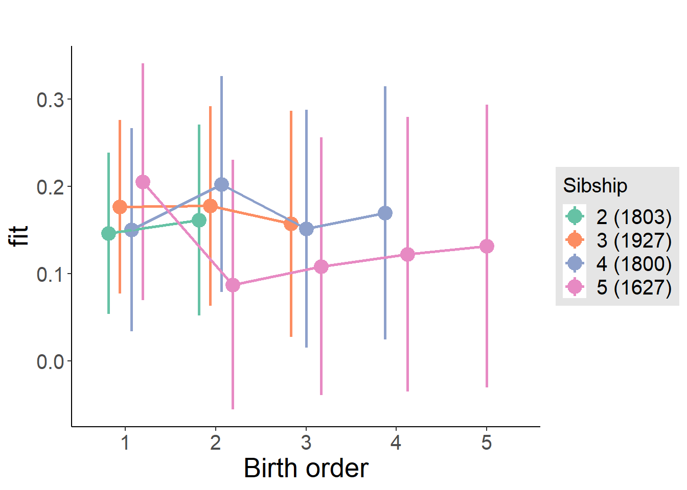
Model Comparison
###### Model 1 - Model 2
anova(m1_covariates_only, m2_birthorder_linear, m3_birthorder_nonlinear, m4_interaction)## refitting model(s) with ML (instead of REML)| Df | AIC | BIC | logLik | deviance | Chisq | Chi Df | Pr(>Chisq) |
|---|---|---|---|---|---|---|---|
| 10 | 19361 | 19430 | -9670 | 19341 | NA | NA | NA |
| 11 | 19363 | 19438 | -9670 | 19341 | 0.3416 | 1 | 0.5589 |
| 14 | 19368 | 19464 | -9670 | 19340 | 0.4585 | 3 | 0.9279 |
| 20 | 19376 | 19513 | -9668 | 19336 | 4.406 | 6 | 0.6219 |
Maternal birth order
outcome_uterus_m1 <- update(m2_birthorder_linear, data = birthorder %>%
mutate(sibling_count = sibling_count_uterus_alive_factor,
birth_order_nonlinear = birthorder_uterus_alive_factor,
birth_order = birthorder_uterus_alive,
count_birth_order = count_birthorder_uterus_alive) %>%
filter(sibling_count != "1"))
compare_models_markdown(outcome_uterus_m1)Basic Model
Model Summary
m1_covariates_only <- update(m2_birthorder_linear, formula = . ~ . - birth_order)
tidy(m1_covariates_only, conf.int = T, conf.level = 0.995)| effect | group | term | estimate | std.error | statistic | df | p.value | conf.low | conf.high |
|---|---|---|---|---|---|---|---|---|---|
| fixed | NA | (Intercept) | 0.3288 | 0.4976 | 0.6608 | 4502 | 0.5088 | -1.068 | 1.726 |
| fixed | NA | poly(age, 3, raw = TRUE)1 | 0.005066 | 0.05809 | 0.08722 | 4505 | 0.9305 | -0.158 | 0.1681 |
| fixed | NA | poly(age, 3, raw = TRUE)2 | -0.0000285 | 0.002141 | -0.01331 | 4507 | 0.9894 | -0.006039 | 0.005982 |
| fixed | NA | poly(age, 3, raw = TRUE)3 | -0.000003809 | 0.00002509 | -0.1518 | 4507 | 0.8794 | -0.00007424 | 0.00006662 |
| fixed | NA | male | -0.1418 | 0.02676 | -5.301 | 4424 | 0.000000121 | -0.2169 | -0.06672 |
| fixed | NA | sibling_count3 | 0.03656 | 0.03684 | 0.9923 | 3311 | 0.3211 | -0.06686 | 0.14 |
| fixed | NA | sibling_count4 | -0.08719 | 0.03984 | -2.188 | 2907 | 0.02872 | -0.199 | 0.02465 |
| fixed | NA | sibling_count5 | -0.1082 | 0.04556 | -2.374 | 2596 | 0.01765 | -0.2361 | 0.01971 |
| ran_pars | mother_pidlink | sd__(Intercept) | 0.3383 | NA | NA | NA | NA | NA | NA |
| ran_pars | Residual | sd__Observation | 0.8393 | NA | NA | NA | NA | NA | NA |
Coefficient Plot
plot(allEffects(m1_covariates_only, confidence.level = 0.995))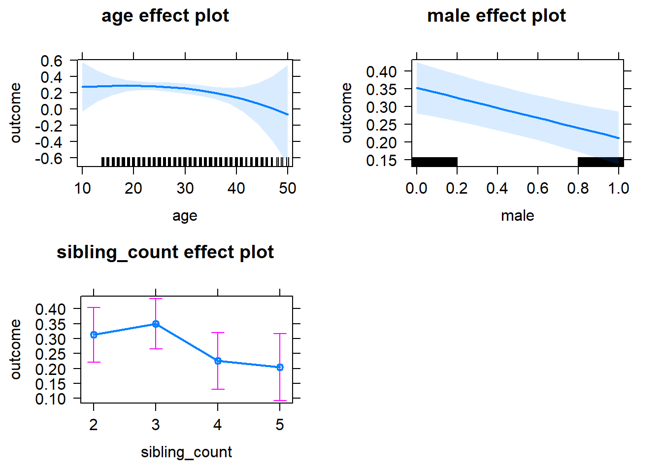
Add Birth Order Linear
Model Summary
tidy(m2_birthorder_linear, conf.int = T, conf.level = 0.995)| effect | group | term | estimate | std.error | statistic | df | p.value | conf.low | conf.high |
|---|---|---|---|---|---|---|---|---|---|
| fixed | NA | (Intercept) | 0.3524 | 0.4982 | 0.7074 | 4501 | 0.4794 | -1.046 | 1.751 |
| fixed | NA | birth_order | -0.01366 | 0.01402 | -0.9748 | 4148 | 0.3297 | -0.05301 | 0.02568 |
| fixed | NA | poly(age, 3, raw = TRUE)1 | 0.004233 | 0.0581 | 0.07286 | 4504 | 0.9419 | -0.1588 | 0.1673 |
| fixed | NA | poly(age, 3, raw = TRUE)2 | 0.00001682 | 0.002142 | 0.007852 | 4506 | 0.9937 | -0.005995 | 0.006029 |
| fixed | NA | poly(age, 3, raw = TRUE)3 | -0.000004621 | 0.00002511 | -0.1841 | 4506 | 0.854 | -0.00007509 | 0.00006585 |
| fixed | NA | male | -0.1414 | 0.02676 | -5.283 | 4422 | 0.0000001334 | -0.2165 | -0.06625 |
| fixed | NA | sibling_count3 | 0.04283 | 0.03741 | 1.145 | 3372 | 0.2523 | -0.06217 | 0.1478 |
| fixed | NA | sibling_count4 | -0.0727 | 0.04253 | -1.709 | 3135 | 0.08749 | -0.1921 | 0.04669 |
| fixed | NA | sibling_count5 | -0.08396 | 0.0519 | -1.618 | 3112 | 0.1059 | -0.2297 | 0.06174 |
| ran_pars | mother_pidlink | sd__(Intercept) | 0.3388 | NA | NA | NA | NA | NA | NA |
| ran_pars | Residual | sd__Observation | 0.8391 | NA | NA | NA | NA | NA | NA |
Coefficient Plot
plot_birthorder2(m2_birthorder_linear, separate = FALSE)
Add Birth Order Factor
Model Summary
m3_birthorder_nonlinear = update(m1_covariates_only, formula = . ~ . + birth_order_nonlinear)
tidy(m3_birthorder_nonlinear, conf.int = T, conf.level = 0.995)| effect | group | term | estimate | std.error | statistic | df | p.value | conf.low | conf.high |
|---|---|---|---|---|---|---|---|---|---|
| fixed | NA | (Intercept) | 0.3302 | 0.4988 | 0.6619 | 4501 | 0.5081 | -1.07 | 1.73 |
| fixed | NA | poly(age, 3, raw = TRUE)1 | 0.005404 | 0.05817 | 0.0929 | 4502 | 0.926 | -0.1579 | 0.1687 |
| fixed | NA | poly(age, 3, raw = TRUE)2 | -0.00002355 | 0.002144 | -0.01098 | 4503 | 0.9912 | -0.006043 | 0.005996 |
| fixed | NA | poly(age, 3, raw = TRUE)3 | -0.000004222 | 0.00002513 | -0.168 | 4503 | 0.8666 | -0.00007477 | 0.00006633 |
| fixed | NA | male | -0.1411 | 0.02677 | -5.271 | 4418 | 0.0000001418 | -0.2163 | -0.06597 |
| fixed | NA | sibling_count3 | 0.03586 | 0.03798 | 0.9441 | 3490 | 0.3452 | -0.07076 | 0.1425 |
| fixed | NA | sibling_count4 | -0.07382 | 0.04316 | -1.71 | 3237 | 0.08729 | -0.195 | 0.04733 |
| fixed | NA | sibling_count5 | -0.08279 | 0.05278 | -1.568 | 3206 | 0.1169 | -0.231 | 0.06538 |
| fixed | NA | birth_order_nonlinear2 | -0.01819 | 0.03171 | -0.5736 | 3587 | 0.5663 | -0.1072 | 0.07081 |
| fixed | NA | birth_order_nonlinear3 | 0.003378 | 0.04045 | 0.08351 | 3801 | 0.9335 | -0.1102 | 0.1169 |
| fixed | NA | birth_order_nonlinear4 | -0.06973 | 0.05442 | -1.281 | 3984 | 0.2001 | -0.2225 | 0.08303 |
| fixed | NA | birth_order_nonlinear5 | -0.06116 | 0.08469 | -0.7222 | 3838 | 0.4702 | -0.2989 | 0.1766 |
| ran_pars | mother_pidlink | sd__(Intercept) | 0.3392 | NA | NA | NA | NA | NA | NA |
| ran_pars | Residual | sd__Observation | 0.8391 | NA | NA | NA | NA | NA | NA |
Coefficient Plot
plot_birthorder(m3_birthorder_nonlinear, separate = FALSE)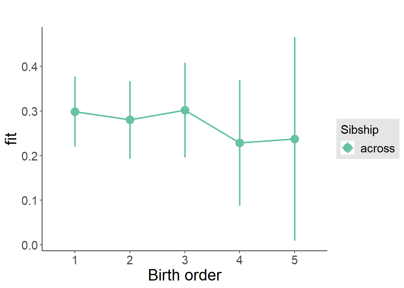
Add Interaction
Model Summary
m4_interaction = update(m3_birthorder_nonlinear, formula = . ~ . - birth_order_nonlinear - sibling_count + count_birth_order)
tidy(m4_interaction, conf.int = T, conf.level = 0.995)| effect | group | term | estimate | std.error | statistic | df | p.value | conf.low | conf.high |
|---|---|---|---|---|---|---|---|---|---|
| fixed | NA | (Intercept) | 0.3367 | 0.4992 | 0.6745 | 4495 | 0.5001 | -1.065 | 1.738 |
| fixed | NA | poly(age, 3, raw = TRUE)1 | 0.005142 | 0.05822 | 0.08833 | 4496 | 0.9296 | -0.1583 | 0.1686 |
| fixed | NA | poly(age, 3, raw = TRUE)2 | -0.00002064 | 0.002146 | -0.009616 | 4497 | 0.9923 | -0.006045 | 0.006004 |
| fixed | NA | poly(age, 3, raw = TRUE)3 | -0.000004154 | 0.00002516 | -0.1651 | 4497 | 0.8689 | -0.00007477 | 0.00006647 |
| fixed | NA | male | -0.1405 | 0.0268 | -5.242 | 4412 | 0.0000001659 | -0.2157 | -0.06526 |
| fixed | NA | count_birth_order2/2 | -0.02885 | 0.05451 | -0.5292 | 3803 | 0.5967 | -0.1818 | 0.1242 |
| fixed | NA | count_birth_order1/3 | 0.03917 | 0.04843 | 0.8089 | 4484 | 0.4186 | -0.09676 | 0.1751 |
| fixed | NA | count_birth_order2/3 | 0.02527 | 0.05285 | 0.4781 | 4497 | 0.6326 | -0.1231 | 0.1736 |
| fixed | NA | count_birth_order3/3 | 0.006197 | 0.05903 | 0.105 | 4491 | 0.9164 | -0.1595 | 0.1719 |
| fixed | NA | count_birth_order1/4 | -0.09156 | 0.05942 | -1.541 | 4494 | 0.1234 | -0.2583 | 0.07522 |
| fixed | NA | count_birth_order2/4 | -0.1156 | 0.06128 | -1.886 | 4496 | 0.05938 | -0.2876 | 0.05646 |
| fixed | NA | count_birth_order3/4 | -0.04838 | 0.06465 | -0.7484 | 4479 | 0.4543 | -0.2298 | 0.1331 |
| fixed | NA | count_birth_order4/4 | -0.1291 | 0.06724 | -1.921 | 4475 | 0.05485 | -0.3179 | 0.05961 |
| fixed | NA | count_birth_order1/5 | -0.1032 | 0.08074 | -1.278 | 4490 | 0.2012 | -0.3299 | 0.1234 |
| fixed | NA | count_birth_order2/5 | -0.0768 | 0.08614 | -0.8916 | 4459 | 0.3727 | -0.3186 | 0.165 |
| fixed | NA | count_birth_order3/5 | -0.06275 | 0.08069 | -0.7777 | 4456 | 0.4368 | -0.2892 | 0.1637 |
| fixed | NA | count_birth_order4/5 | -0.1806 | 0.0777 | -2.325 | 4467 | 0.02014 | -0.3987 | 0.03748 |
| fixed | NA | count_birth_order5/5 | -0.1476 | 0.08078 | -1.827 | 4450 | 0.06781 | -0.3743 | 0.07919 |
| ran_pars | mother_pidlink | sd__(Intercept) | 0.3383 | NA | NA | NA | NA | NA | NA |
| ran_pars | Residual | sd__Observation | 0.8399 | NA | NA | NA | NA | NA | NA |
Coefficient Plot
plot_birthorder(m4_interaction)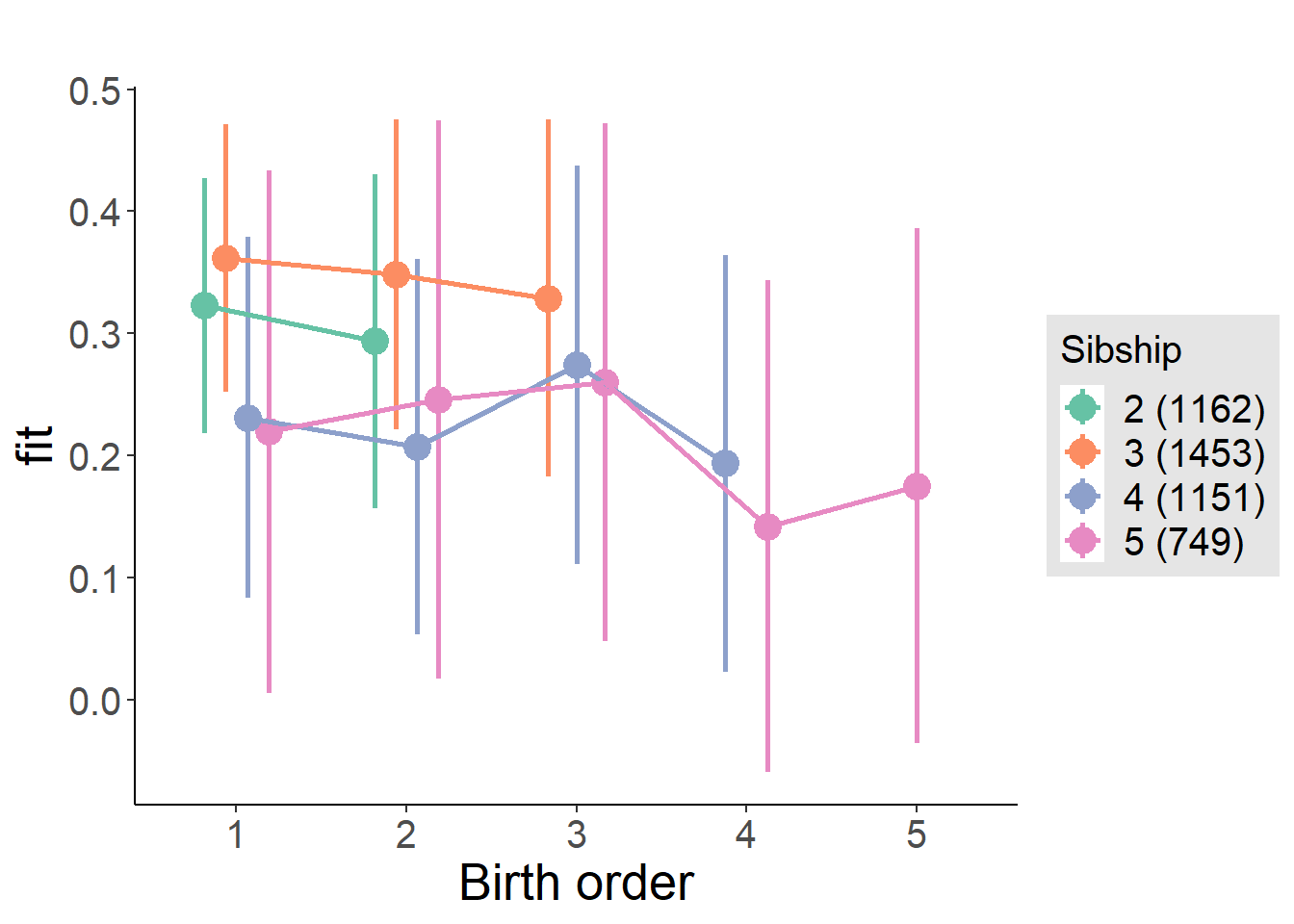
Model Comparison
###### Model 1 - Model 2
anova(m1_covariates_only, m2_birthorder_linear, m3_birthorder_nonlinear, m4_interaction)## refitting model(s) with ML (instead of REML)| Df | AIC | BIC | logLik | deviance | Chisq | Chi Df | Pr(>Chisq) |
|---|---|---|---|---|---|---|---|
| 10 | 11889 | 11953 | -5935 | 11869 | NA | NA | NA |
| 11 | 11890 | 11961 | -5934 | 11868 | 0.9504 | 1 | 0.3296 |
| 14 | 11895 | 11985 | -5933 | 11867 | 1.325 | 3 | 0.7232 |
| 20 | 11905 | 12034 | -5933 | 11865 | 1.494 | 6 | 0.9599 |
Maternal pregnancy order
outcome_preg_m1 <- update(m2_birthorder_linear, data = birthorder %>%
mutate(sibling_count = sibling_count_uterus_preg_factor,
birth_order_nonlinear = birthorder_uterus_preg_factor,
birth_order = birthorder_uterus_preg,
count_birth_order = count_birthorder_uterus_preg
) %>%
filter(sibling_count != "1"))
compare_models_markdown(outcome_preg_m1)Basic Model
Model Summary
m1_covariates_only <- update(m2_birthorder_linear, formula = . ~ . - birth_order)
tidy(m1_covariates_only, conf.int = T, conf.level = 0.995)| effect | group | term | estimate | std.error | statistic | df | p.value | conf.low | conf.high |
|---|---|---|---|---|---|---|---|---|---|
| fixed | NA | (Intercept) | 0.4567 | 0.5104 | 0.8949 | 4176 | 0.3709 | -0.9759 | 1.889 |
| fixed | NA | poly(age, 3, raw = TRUE)1 | -0.009468 | 0.05963 | -0.1588 | 4179 | 0.8738 | -0.1768 | 0.1579 |
| fixed | NA | poly(age, 3, raw = TRUE)2 | 0.0004898 | 0.002199 | 0.2227 | 4182 | 0.8237 | -0.005682 | 0.006662 |
| fixed | NA | poly(age, 3, raw = TRUE)3 | -0.00001023 | 0.00002577 | -0.3971 | 4183 | 0.6913 | -0.00008258 | 0.00006211 |
| fixed | NA | male | -0.1367 | 0.02765 | -4.944 | 4092 | 0.000000797 | -0.2143 | -0.05909 |
| fixed | NA | sibling_count3 | 0.03155 | 0.03975 | 0.7937 | 3150 | 0.4274 | -0.08004 | 0.1431 |
| fixed | NA | sibling_count4 | -0.06652 | 0.04207 | -1.581 | 2868 | 0.1139 | -0.1846 | 0.05157 |
| fixed | NA | sibling_count5 | -0.04892 | 0.04517 | -1.083 | 2575 | 0.2788 | -0.1757 | 0.07787 |
| ran_pars | mother_pidlink | sd__(Intercept) | 0.3464 | NA | NA | NA | NA | NA | NA |
| ran_pars | Residual | sd__Observation | 0.8322 | NA | NA | NA | NA | NA | NA |
Coefficient Plot
plot(allEffects(m1_covariates_only, confidence.level = 0.995))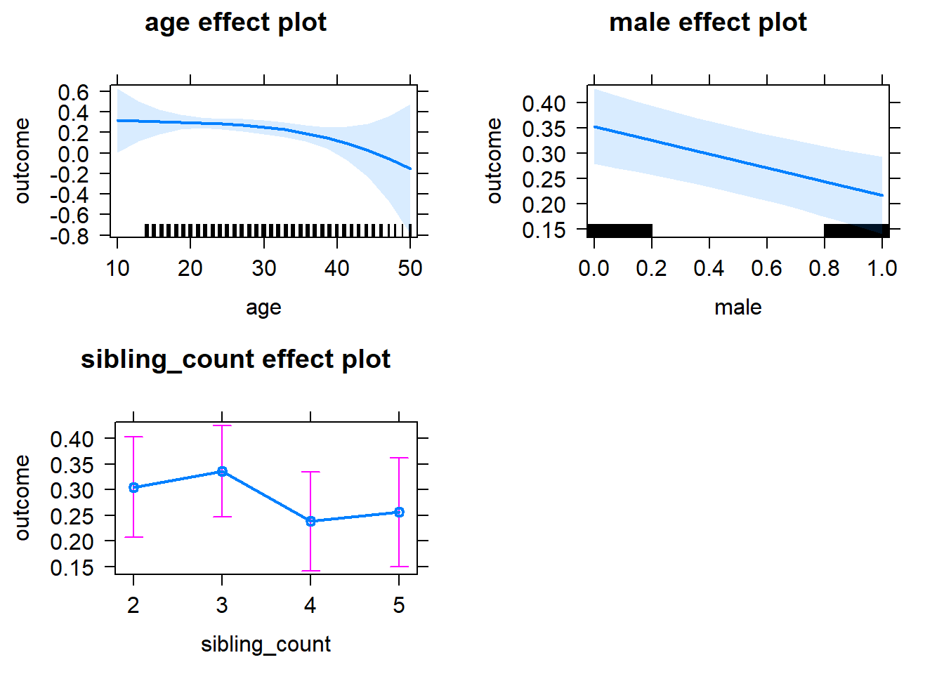
Add Birth Order Linear
Model Summary
tidy(m2_birthorder_linear, conf.int = T, conf.level = 0.995)| effect | group | term | estimate | std.error | statistic | df | p.value | conf.low | conf.high |
|---|---|---|---|---|---|---|---|---|---|
| fixed | NA | (Intercept) | 0.4924 | 0.5108 | 0.9639 | 4174 | 0.3351 | -0.9415 | 1.926 |
| fixed | NA | birth_order | -0.02118 | 0.01399 | -1.514 | 3917 | 0.1302 | -0.06045 | 0.01809 |
| fixed | NA | poly(age, 3, raw = TRUE)1 | -0.01057 | 0.05962 | -0.1772 | 4178 | 0.8594 | -0.1779 | 0.1568 |
| fixed | NA | poly(age, 3, raw = TRUE)2 | 0.0005504 | 0.002199 | 0.2503 | 4181 | 0.8023 | -0.005622 | 0.006723 |
| fixed | NA | poly(age, 3, raw = TRUE)3 | -0.00001137 | 0.00002578 | -0.4411 | 4182 | 0.6592 | -0.00008373 | 0.00006099 |
| fixed | NA | male | -0.1363 | 0.02765 | -4.928 | 4091 | 0.0000008635 | -0.2139 | -0.05865 |
| fixed | NA | sibling_count3 | 0.04126 | 0.04026 | 1.025 | 3193 | 0.3056 | -0.07177 | 0.1543 |
| fixed | NA | sibling_count4 | -0.04482 | 0.04444 | -1.008 | 3035 | 0.3133 | -0.1696 | 0.07994 |
| fixed | NA | sibling_count5 | -0.01422 | 0.05065 | -0.2809 | 2967 | 0.7788 | -0.1564 | 0.1279 |
| ran_pars | mother_pidlink | sd__(Intercept) | 0.3468 | NA | NA | NA | NA | NA | NA |
| ran_pars | Residual | sd__Observation | 0.8319 | NA | NA | NA | NA | NA | NA |
Coefficient Plot
plot_birthorder2(m2_birthorder_linear, separate = FALSE)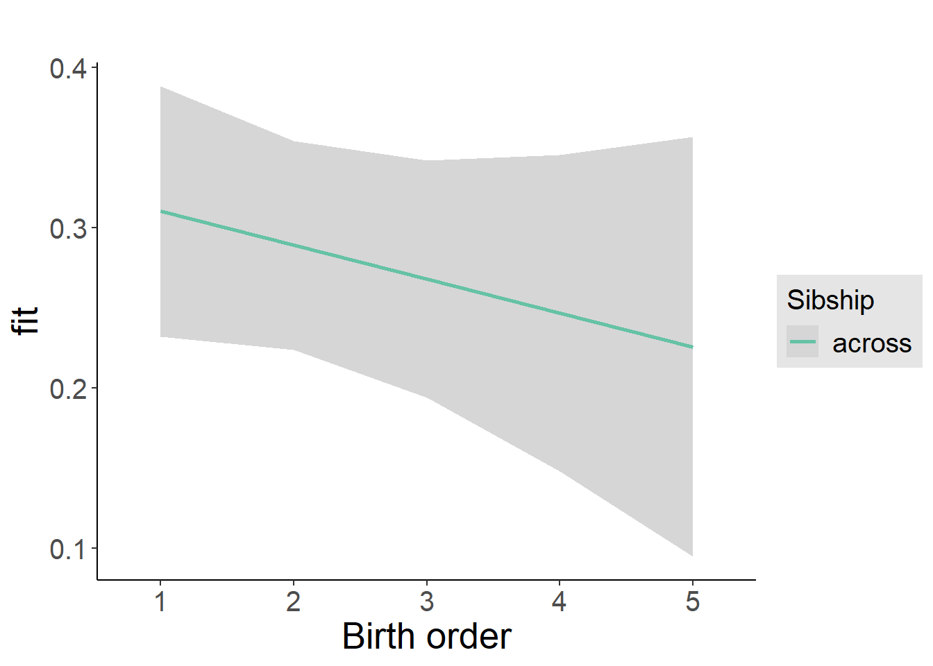
Add Birth Order Factor
Model Summary
m3_birthorder_nonlinear = update(m1_covariates_only, formula = . ~ . + birth_order_nonlinear)
tidy(m3_birthorder_nonlinear, conf.int = T, conf.level = 0.995)| effect | group | term | estimate | std.error | statistic | df | p.value | conf.low | conf.high |
|---|---|---|---|---|---|---|---|---|---|
| fixed | NA | (Intercept) | 0.4382 | 0.5113 | 0.8569 | 4175 | 0.3915 | -0.9972 | 1.873 |
| fixed | NA | poly(age, 3, raw = TRUE)1 | -0.007412 | 0.05969 | -0.1242 | 4177 | 0.9012 | -0.175 | 0.1601 |
| fixed | NA | poly(age, 3, raw = TRUE)2 | 0.0004352 | 0.002201 | 0.1977 | 4179 | 0.8433 | -0.005744 | 0.006614 |
| fixed | NA | poly(age, 3, raw = TRUE)3 | -0.0000101 | 0.0000258 | -0.3915 | 4179 | 0.6955 | -0.00008253 | 0.00006233 |
| fixed | NA | male | -0.136 | 0.02766 | -4.918 | 4087 | 0.0000009066 | -0.2137 | -0.0584 |
| fixed | NA | sibling_count3 | 0.03449 | 0.04084 | 0.8446 | 3292 | 0.3984 | -0.08015 | 0.1491 |
| fixed | NA | sibling_count4 | -0.0512 | 0.04505 | -1.136 | 3124 | 0.2559 | -0.1777 | 0.07526 |
| fixed | NA | sibling_count5 | -0.006314 | 0.05116 | -0.1234 | 3020 | 0.9018 | -0.1499 | 0.1373 |
| fixed | NA | birth_order_nonlinear2 | -0.001131 | 0.03283 | -0.03445 | 3370 | 0.9725 | -0.09328 | 0.09102 |
| fixed | NA | birth_order_nonlinear3 | -0.01076 | 0.04158 | -0.2587 | 3579 | 0.7959 | -0.1275 | 0.106 |
| fixed | NA | birth_order_nonlinear4 | -0.05773 | 0.05512 | -1.047 | 3728 | 0.295 | -0.2125 | 0.09699 |
| fixed | NA | birth_order_nonlinear5 | -0.1495 | 0.08072 | -1.852 | 3605 | 0.06414 | -0.3761 | 0.07711 |
| ran_pars | mother_pidlink | sd__(Intercept) | 0.3473 | NA | NA | NA | NA | NA | NA |
| ran_pars | Residual | sd__Observation | 0.8319 | NA | NA | NA | NA | NA | NA |
Coefficient Plot
plot_birthorder(m3_birthorder_nonlinear, separate = FALSE)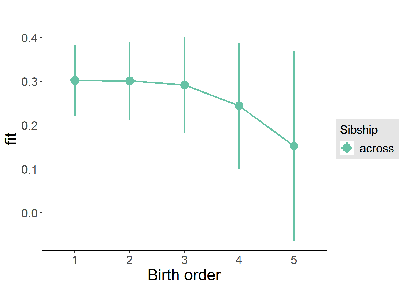
Add Interaction
Model Summary
m4_interaction = update(m3_birthorder_nonlinear, formula = . ~ . - birth_order_nonlinear - sibling_count + count_birth_order)
tidy(m4_interaction, conf.int = T, conf.level = 0.995)| effect | group | term | estimate | std.error | statistic | df | p.value | conf.low | conf.high |
|---|---|---|---|---|---|---|---|---|---|
| fixed | NA | (Intercept) | 0.4422 | 0.5119 | 0.8638 | 4169 | 0.3877 | -0.9948 | 1.879 |
| fixed | NA | poly(age, 3, raw = TRUE)1 | -0.008889 | 0.05974 | -0.1488 | 4171 | 0.8817 | -0.1766 | 0.1588 |
| fixed | NA | poly(age, 3, raw = TRUE)2 | 0.0004942 | 0.002203 | 0.2243 | 4173 | 0.8225 | -0.005691 | 0.006679 |
| fixed | NA | poly(age, 3, raw = TRUE)3 | -0.00001083 | 0.00002583 | -0.4191 | 4173 | 0.6752 | -0.00008335 | 0.00006169 |
| fixed | NA | male | -0.1364 | 0.02769 | -4.928 | 4080 | 0.0000008658 | -0.2142 | -0.05872 |
| fixed | NA | count_birth_order2/2 | 0.0214 | 0.05936 | 0.3605 | 3566 | 0.7185 | -0.1452 | 0.188 |
| fixed | NA | count_birth_order1/3 | 0.05195 | 0.05221 | 0.9949 | 4161 | 0.3198 | -0.09462 | 0.1985 |
| fixed | NA | count_birth_order2/3 | 0.03827 | 0.05659 | 0.6762 | 4173 | 0.4989 | -0.1206 | 0.1971 |
| fixed | NA | count_birth_order3/3 | 0.01518 | 0.06364 | 0.2386 | 4167 | 0.8114 | -0.1635 | 0.1938 |
| fixed | NA | count_birth_order1/4 | -0.06525 | 0.06198 | -1.053 | 4170 | 0.2925 | -0.2392 | 0.1087 |
| fixed | NA | count_birth_order2/4 | -0.05804 | 0.06282 | -0.924 | 4173 | 0.3556 | -0.2344 | 0.1183 |
| fixed | NA | count_birth_order3/4 | -0.03496 | 0.06891 | -0.5074 | 4152 | 0.6119 | -0.2284 | 0.1585 |
| fixed | NA | count_birth_order4/4 | -0.06964 | 0.07108 | -0.9797 | 4152 | 0.3273 | -0.2692 | 0.1299 |
| fixed | NA | count_birth_order1/5 | 0.03193 | 0.07369 | 0.4334 | 4173 | 0.6648 | -0.1749 | 0.2388 |
| fixed | NA | count_birth_order2/5 | 0.001311 | 0.07884 | 0.01663 | 4150 | 0.9867 | -0.22 | 0.2226 |
| fixed | NA | count_birth_order3/5 | -0.009253 | 0.07655 | -0.1209 | 4143 | 0.9038 | -0.2241 | 0.2056 |
| fixed | NA | count_birth_order4/5 | -0.09757 | 0.07925 | -1.231 | 4124 | 0.2183 | -0.32 | 0.1249 |
| fixed | NA | count_birth_order5/5 | -0.149 | 0.07939 | -1.876 | 4122 | 0.06067 | -0.3718 | 0.07388 |
| ran_pars | mother_pidlink | sd__(Intercept) | 0.3473 | NA | NA | NA | NA | NA | NA |
| ran_pars | Residual | sd__Observation | 0.8324 | NA | NA | NA | NA | NA | NA |
Coefficient Plot
plot_birthorder(m4_interaction)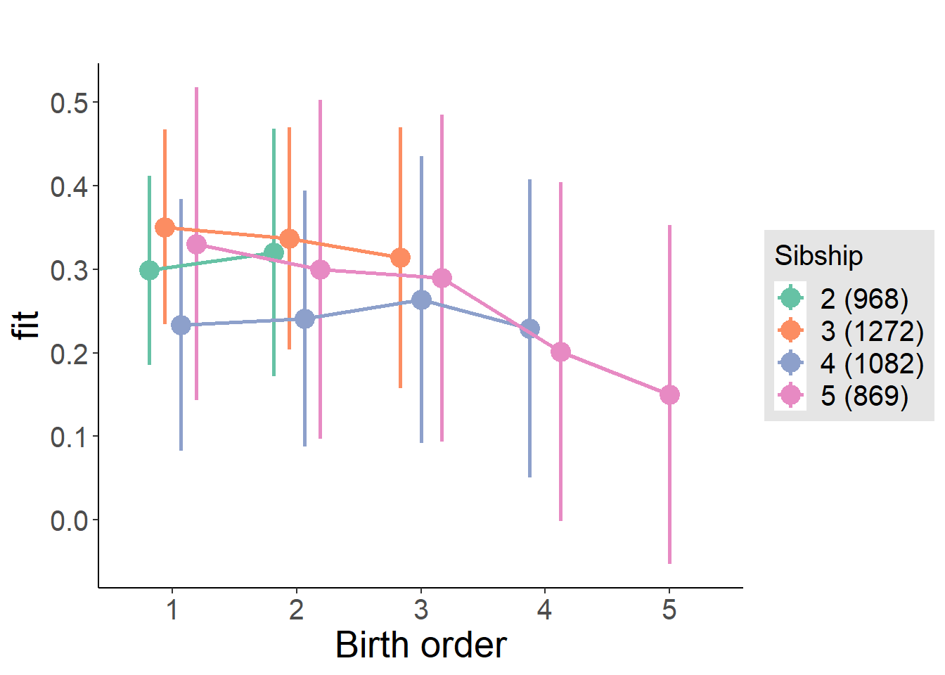
Model Comparison
###### Model 1 - Model 2
anova(m1_covariates_only, m2_birthorder_linear, m3_birthorder_nonlinear, m4_interaction)## refitting model(s) with ML (instead of REML)| Df | AIC | BIC | logLik | deviance | Chisq | Chi Df | Pr(>Chisq) |
|---|---|---|---|---|---|---|---|
| 10 | 11002 | 11065 | -5491 | 10982 | NA | NA | NA |
| 11 | 11002 | 11071 | -5490 | 10980 | 2.294 | 1 | 0.1299 |
| 14 | 11006 | 11095 | -5489 | 10978 | 1.804 | 3 | 0.614 |
| 20 | 11016 | 11143 | -5488 | 10976 | 1.574 | 6 | 0.9544 |
Parental full sibling order
outcome_parental_m1 <- update(m2_birthorder_linear, data = birthorder %>%
mutate(sibling_count = sibling_count_genes_factor,
birth_order_nonlinear = birthorder_genes_factor,
birth_order = birthorder_genes,
count_birth_order = count_birthorder_genes
) %>%
filter(sibling_count != "1"))
compare_models_markdown(outcome_parental_m1)Basic Model
Model Summary
m1_covariates_only <- update(m2_birthorder_linear, formula = . ~ . - birth_order)
tidy(m1_covariates_only, conf.int = T, conf.level = 0.995)| effect | group | term | estimate | std.error | statistic | df | p.value | conf.low | conf.high |
|---|---|---|---|---|---|---|---|---|---|
| fixed | NA | (Intercept) | 0.382 | 0.5014 | 0.7617 | 4487 | 0.4463 | -1.026 | 1.79 |
| fixed | NA | poly(age, 3, raw = TRUE)1 | -0.002567 | 0.05861 | -0.0438 | 4490 | 0.9651 | -0.1671 | 0.162 |
| fixed | NA | poly(age, 3, raw = TRUE)2 | 0.0003015 | 0.002164 | 0.1393 | 4492 | 0.8892 | -0.005772 | 0.006375 |
| fixed | NA | poly(age, 3, raw = TRUE)3 | -0.000008284 | 0.0000254 | -0.3261 | 4492 | 0.7444 | -0.00007959 | 0.00006302 |
| fixed | NA | male | -0.131 | 0.02676 | -4.895 | 4408 | 0.000001017 | -0.2061 | -0.05589 |
| fixed | NA | sibling_count3 | 0.01628 | 0.03633 | 0.448 | 3294 | 0.6542 | -0.08571 | 0.1183 |
| fixed | NA | sibling_count4 | -0.08339 | 0.03951 | -2.11 | 2908 | 0.03491 | -0.1943 | 0.02753 |
| fixed | NA | sibling_count5 | -0.1064 | 0.04665 | -2.282 | 2514 | 0.02259 | -0.2374 | 0.02451 |
| ran_pars | mother_pidlink | sd__(Intercept) | 0.3393 | NA | NA | NA | NA | NA | NA |
| ran_pars | Residual | sd__Observation | 0.8372 | NA | NA | NA | NA | NA | NA |
Coefficient Plot
plot(allEffects(m1_covariates_only, confidence.level = 0.995))
Add Birth Order Linear
Model Summary
tidy(m2_birthorder_linear, conf.int = T, conf.level = 0.995)| effect | group | term | estimate | std.error | statistic | df | p.value | conf.low | conf.high |
|---|---|---|---|---|---|---|---|---|---|
| fixed | NA | (Intercept) | 0.4022 | 0.502 | 0.8012 | 4486 | 0.4231 | -1.007 | 1.811 |
| fixed | NA | birth_order | -0.01191 | 0.01418 | -0.8402 | 4114 | 0.4008 | -0.05171 | 0.02788 |
| fixed | NA | poly(age, 3, raw = TRUE)1 | -0.003238 | 0.05862 | -0.05524 | 4489 | 0.9559 | -0.1678 | 0.1613 |
| fixed | NA | poly(age, 3, raw = TRUE)2 | 0.0003388 | 0.002164 | 0.1565 | 4491 | 0.8756 | -0.005736 | 0.006414 |
| fixed | NA | poly(age, 3, raw = TRUE)3 | -0.000008964 | 0.00002542 | -0.3527 | 4491 | 0.7243 | -0.00008031 | 0.00006238 |
| fixed | NA | male | -0.1307 | 0.02677 | -4.883 | 4406 | 0.000001082 | -0.2058 | -0.05557 |
| fixed | NA | sibling_count3 | 0.02174 | 0.03691 | 0.589 | 3352 | 0.5559 | -0.08188 | 0.1254 |
| fixed | NA | sibling_count4 | -0.0708 | 0.04226 | -1.675 | 3148 | 0.09399 | -0.1894 | 0.04783 |
| fixed | NA | sibling_count5 | -0.08626 | 0.05247 | -1.644 | 2976 | 0.1003 | -0.2335 | 0.06102 |
| ran_pars | mother_pidlink | sd__(Intercept) | 0.3395 | NA | NA | NA | NA | NA | NA |
| ran_pars | Residual | sd__Observation | 0.8372 | NA | NA | NA | NA | NA | NA |
Coefficient Plot
plot_birthorder2(m2_birthorder_linear, separate = FALSE)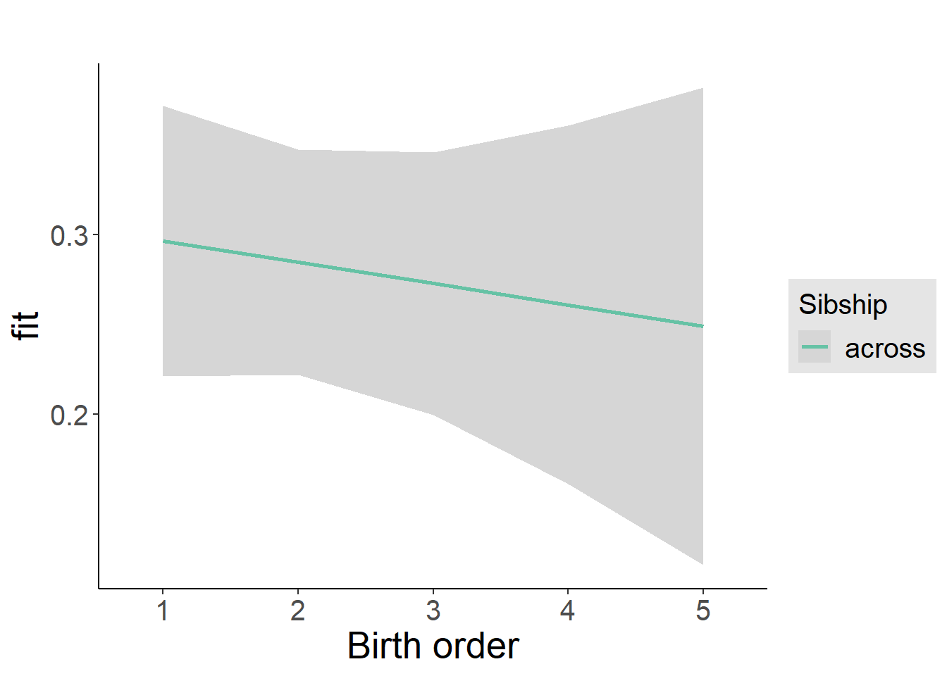
Add Birth Order Factor
Model Summary
m3_birthorder_nonlinear = update(m1_covariates_only, formula = . ~ . + birth_order_nonlinear)
tidy(m3_birthorder_nonlinear, conf.int = T, conf.level = 0.995)| effect | group | term | estimate | std.error | statistic | df | p.value | conf.low | conf.high |
|---|---|---|---|---|---|---|---|---|---|
| fixed | NA | (Intercept) | 0.3786 | 0.5026 | 0.7534 | 4486 | 0.4513 | -1.032 | 1.789 |
| fixed | NA | poly(age, 3, raw = TRUE)1 | -0.001463 | 0.05869 | -0.02493 | 4487 | 0.9801 | -0.1662 | 0.1633 |
| fixed | NA | poly(age, 3, raw = TRUE)2 | 0.0002766 | 0.002167 | 0.1277 | 4488 | 0.8984 | -0.005805 | 0.006358 |
| fixed | NA | poly(age, 3, raw = TRUE)3 | -0.000008318 | 0.00002544 | -0.327 | 4488 | 0.7437 | -0.00007974 | 0.0000631 |
| fixed | NA | male | -0.1301 | 0.02677 | -4.861 | 4401 | 0.000001209 | -0.2053 | -0.05499 |
| fixed | NA | sibling_count3 | 0.01266 | 0.03751 | 0.3374 | 3474 | 0.7359 | -0.09264 | 0.118 |
| fixed | NA | sibling_count4 | -0.07595 | 0.0429 | -1.77 | 3251 | 0.07676 | -0.1964 | 0.04447 |
| fixed | NA | sibling_count5 | -0.08292 | 0.05354 | -1.549 | 3081 | 0.1215 | -0.2332 | 0.06737 |
| fixed | NA | birth_order_nonlinear2 | -0.02296 | 0.03146 | -0.7298 | 3568 | 0.4656 | -0.1113 | 0.06535 |
| fixed | NA | birth_order_nonlinear3 | 0.01392 | 0.04024 | 0.346 | 3760 | 0.7294 | -0.09902 | 0.1269 |
| fixed | NA | birth_order_nonlinear4 | -0.05674 | 0.05549 | -1.023 | 3947 | 0.3066 | -0.2125 | 0.09902 |
| fixed | NA | birth_order_nonlinear5 | -0.08854 | 0.09055 | -0.9778 | 3882 | 0.3282 | -0.3427 | 0.1656 |
| ran_pars | mother_pidlink | sd__(Intercept) | 0.3409 | NA | NA | NA | NA | NA | NA |
| ran_pars | Residual | sd__Observation | 0.8368 | NA | NA | NA | NA | NA | NA |
Coefficient Plot
plot_birthorder(m3_birthorder_nonlinear, separate = FALSE)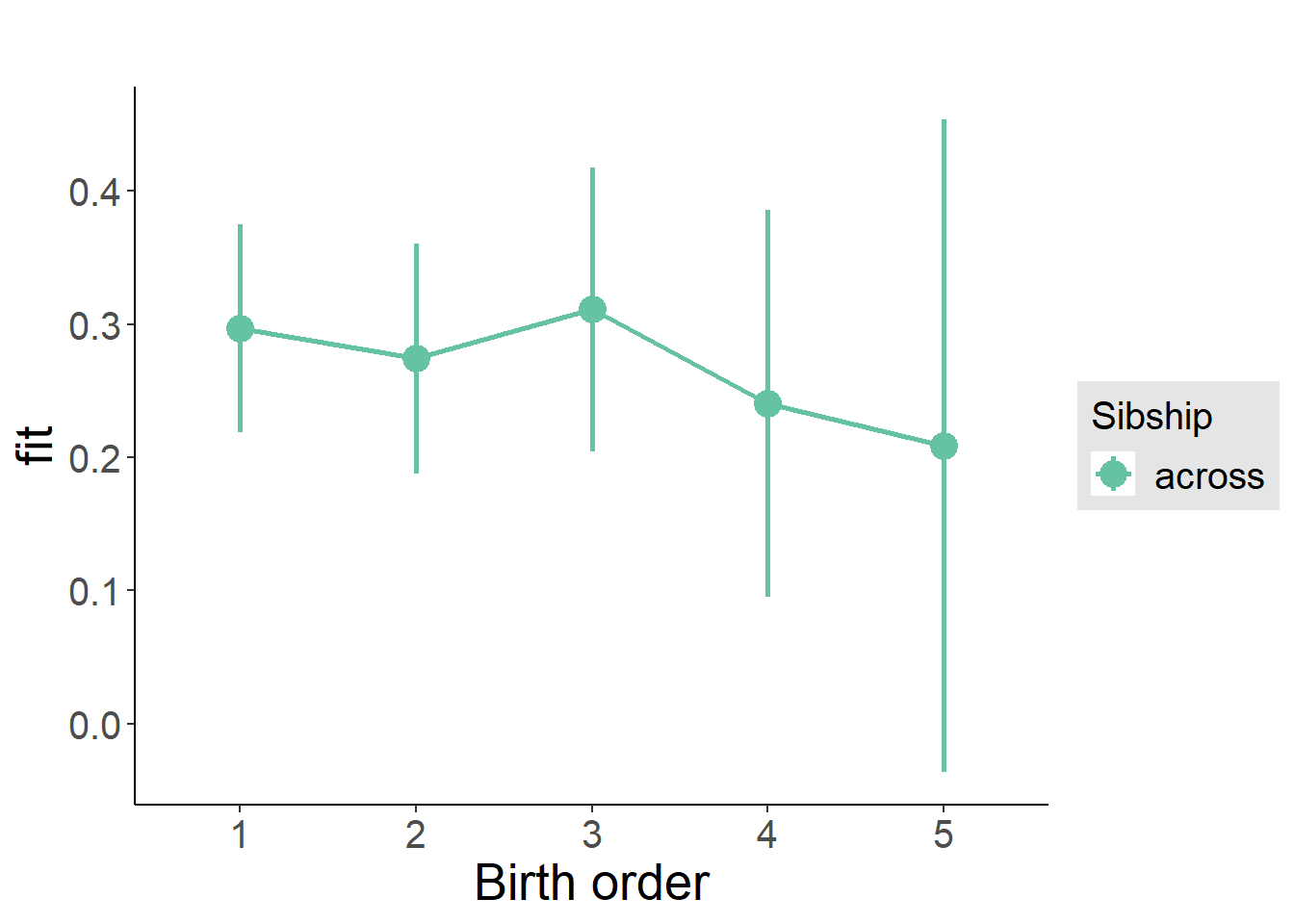
Add Interaction
Model Summary
m4_interaction = update(m3_birthorder_nonlinear, formula = . ~ . - birth_order_nonlinear - sibling_count + count_birth_order)
tidy(m4_interaction, conf.int = T, conf.level = 0.995)| effect | group | term | estimate | std.error | statistic | df | p.value | conf.low | conf.high |
|---|---|---|---|---|---|---|---|---|---|
| fixed | NA | (Intercept) | 0.3787 | 0.503 | 0.7529 | 4480 | 0.4515 | -1.033 | 1.791 |
| fixed | NA | poly(age, 3, raw = TRUE)1 | -0.001063 | 0.05874 | -0.0181 | 4481 | 0.9856 | -0.166 | 0.1638 |
| fixed | NA | poly(age, 3, raw = TRUE)2 | 0.0002579 | 0.002169 | 0.1189 | 4482 | 0.9053 | -0.00583 | 0.006345 |
| fixed | NA | poly(age, 3, raw = TRUE)3 | -0.000008047 | 0.00002547 | -0.316 | 4482 | 0.752 | -0.00007954 | 0.00006344 |
| fixed | NA | male | -0.1298 | 0.0268 | -4.842 | 4395 | 0.000001332 | -0.205 | -0.05453 |
| fixed | NA | count_birth_order2/2 | -0.03177 | 0.05298 | -0.5996 | 3754 | 0.5488 | -0.1805 | 0.117 |
| fixed | NA | count_birth_order1/3 | 0.00818 | 0.04777 | 0.1712 | 4467 | 0.864 | -0.1259 | 0.1423 |
| fixed | NA | count_birth_order2/3 | -0.003009 | 0.05274 | -0.05706 | 4482 | 0.9545 | -0.1511 | 0.145 |
| fixed | NA | count_birth_order3/3 | 0.01269 | 0.05789 | 0.2192 | 4474 | 0.8265 | -0.1498 | 0.1752 |
| fixed | NA | count_birth_order1/4 | -0.07253 | 0.05958 | -1.217 | 4481 | 0.2236 | -0.2398 | 0.09472 |
| fixed | NA | count_birth_order2/4 | -0.1148 | 0.06107 | -1.879 | 4479 | 0.06025 | -0.2862 | 0.05665 |
| fixed | NA | count_birth_order3/4 | -0.05902 | 0.06386 | -0.9243 | 4460 | 0.3554 | -0.2383 | 0.1202 |
| fixed | NA | count_birth_order4/4 | -0.1354 | 0.06754 | -2.004 | 4451 | 0.04511 | -0.3249 | 0.05422 |
| fixed | NA | count_birth_order1/5 | -0.1097 | 0.08044 | -1.363 | 4479 | 0.1729 | -0.3355 | 0.1161 |
| fixed | NA | count_birth_order2/5 | -0.09573 | 0.08861 | -1.08 | 4439 | 0.28 | -0.3445 | 0.153 |
| fixed | NA | count_birth_order3/5 | -0.05593 | 0.08442 | -0.6626 | 4434 | 0.5076 | -0.2929 | 0.181 |
| fixed | NA | count_birth_order4/5 | -0.1428 | 0.08132 | -1.756 | 4448 | 0.07909 | -0.3711 | 0.08543 |
| fixed | NA | count_birth_order5/5 | -0.1742 | 0.08632 | -2.018 | 4431 | 0.04363 | -0.4165 | 0.06809 |
| ran_pars | mother_pidlink | sd__(Intercept) | 0.3402 | NA | NA | NA | NA | NA | NA |
| ran_pars | Residual | sd__Observation | 0.8376 | NA | NA | NA | NA | NA | NA |
Coefficient Plot
plot_birthorder(m4_interaction)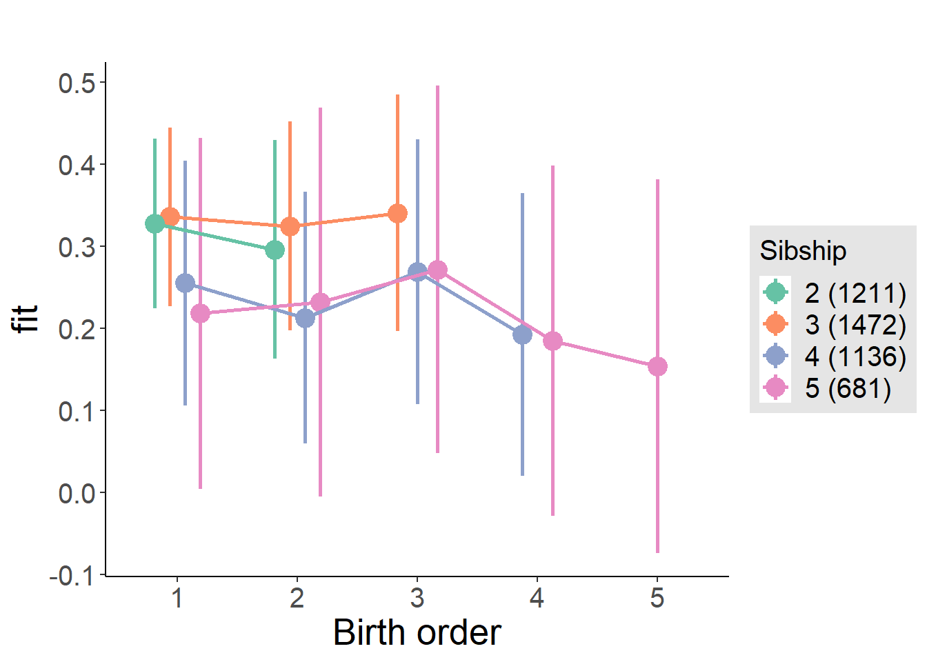
Model Comparison
###### Model 1 - Model 2
anova(m1_covariates_only, m2_birthorder_linear, m3_birthorder_nonlinear, m4_interaction)## refitting model(s) with ML (instead of REML)| Df | AIC | BIC | logLik | deviance | Chisq | Chi Df | Pr(>Chisq) |
|---|---|---|---|---|---|---|---|
| 10 | 11833 | 11897 | -5907 | 11813 | NA | NA | NA |
| 11 | 11835 | 11905 | -5906 | 11813 | 0.7062 | 1 | 0.4007 |
| 14 | 11839 | 11928 | -5905 | 11811 | 1.968 | 3 | 0.5792 |
| 20 | 11850 | 11978 | -5905 | 11810 | 0.4314 | 6 | 0.9986 |
Compare birth order specifications
library(coefplot)
multiplot(outcome_naive_m1, outcome_preg_m1, outcome_uterus_m1, outcome_parental_m1, dodgeHeight = 0.6,
intercept = FALSE)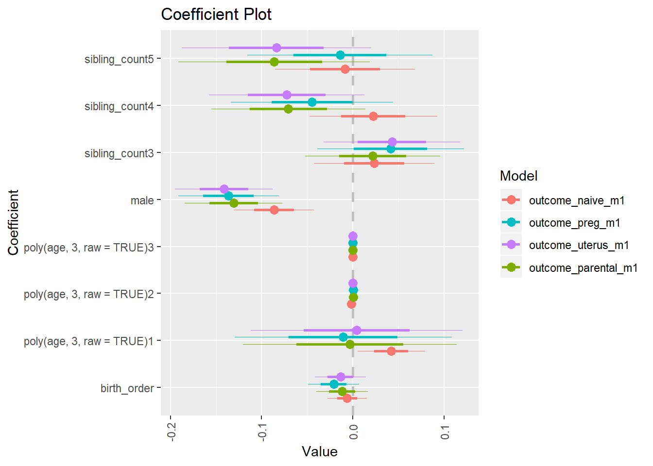
Delayed word recall
birthorder <- birthorder %>% mutate(outcome = words_delayed)
model = lmer(outcome ~ birth_order + poly(age, 3, raw = TRUE) + male + sibling_count + (1 | mother_pidlink),
data = birthorder)
compare_birthorder_specs(model)Naive birth order
outcome_naive_m1 <- update(m2_birthorder_linear, data = birthorder %>%
mutate(sibling_count = sibling_count_naive_factor,
birth_order_nonlinear = birthorder_naive_factor,
birth_order = birthorder_naive,
count_birth_order = count_birthorder_naive) %>%
filter(sibling_count != "1"))
compare_models_markdown(outcome_naive_m1)Basic Model
Model Summary
m1_covariates_only <- update(m2_birthorder_linear, formula = . ~ . - birth_order)
tidy(m1_covariates_only, conf.int = T, conf.level = 0.995)| effect | group | term | estimate | std.error | statistic | df | p.value | conf.low | conf.high |
|---|---|---|---|---|---|---|---|---|---|
| fixed | NA | (Intercept) | 0.1677 | 0.1929 | 0.8695 | 6924 | 0.3846 | -0.3737 | 0.709 |
| fixed | NA | poly(age, 3, raw = TRUE)1 | 0.03045 | 0.01856 | 1.64 | 6814 | 0.101 | -0.02166 | 0.08255 |
| fixed | NA | poly(age, 3, raw = TRUE)2 | -0.001281 | 0.0005433 | -2.358 | 6667 | 0.01842 | -0.002806 | 0.0002442 |
| fixed | NA | poly(age, 3, raw = TRUE)3 | 0.00000719 | 0.000004938 | 1.456 | 6541 | 0.1454 | -0.000006671 | 0.00002105 |
| fixed | NA | male | -0.07999 | 0.02212 | -3.617 | 6905 | 0.0003002 | -0.1421 | -0.01791 |
| fixed | NA | sibling_count3 | 0.04555 | 0.03279 | 1.389 | 5003 | 0.1648 | -0.04648 | 0.1376 |
| fixed | NA | sibling_count4 | 0.02904 | 0.03394 | 0.8554 | 4558 | 0.3923 | -0.06624 | 0.1243 |
| fixed | NA | sibling_count5 | -0.00268 | 0.03548 | -0.07554 | 4089 | 0.9398 | -0.1023 | 0.09691 |
| ran_pars | mother_pidlink | sd__(Intercept) | 0.4083 | NA | NA | NA | NA | NA | NA |
| ran_pars | Residual | sd__Observation | 0.8571 | NA | NA | NA | NA | NA | NA |
Coefficient Plot
plot(allEffects(m1_covariates_only, confidence.level = 0.995))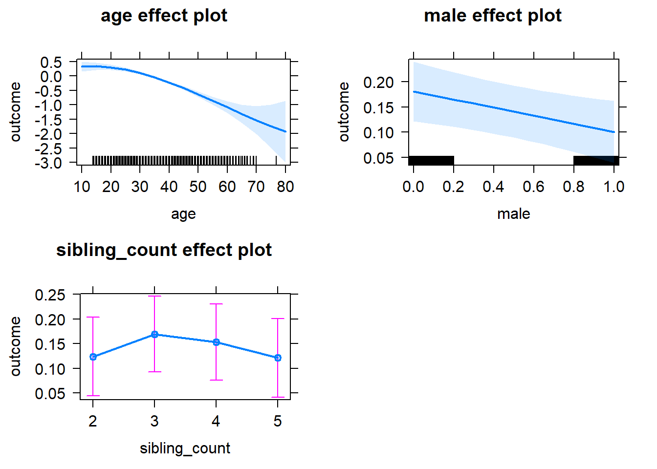
Add Birth Order Linear
Model Summary
tidy(m2_birthorder_linear, conf.int = T, conf.level = 0.995)| effect | group | term | estimate | std.error | statistic | df | p.value | conf.low | conf.high |
|---|---|---|---|---|---|---|---|---|---|
| fixed | NA | (Intercept) | 0.1646 | 0.1929 | 0.8529 | 6911 | 0.3938 | -0.377 | 0.7062 |
| fixed | NA | birth_order | 0.006134 | 0.01092 | 0.5618 | 5892 | 0.5743 | -0.02451 | 0.03678 |
| fixed | NA | poly(age, 3, raw = TRUE)1 | 0.02988 | 0.01859 | 1.608 | 6834 | 0.108 | -0.0223 | 0.08207 |
| fixed | NA | poly(age, 3, raw = TRUE)2 | -0.001266 | 0.000544 | -2.327 | 6679 | 0.01998 | -0.002793 | 0.000261 |
| fixed | NA | poly(age, 3, raw = TRUE)3 | 0.000007093 | 0.000004941 | 1.435 | 6547 | 0.1512 | -0.000006777 | 0.00002096 |
| fixed | NA | male | -0.08016 | 0.02212 | -3.624 | 6903 | 0.0002924 | -0.1422 | -0.01807 |
| fixed | NA | sibling_count3 | 0.04344 | 0.033 | 1.316 | 5121 | 0.1881 | -0.04919 | 0.1361 |
| fixed | NA | sibling_count4 | 0.02405 | 0.03509 | 0.6854 | 5052 | 0.4931 | -0.07444 | 0.1225 |
| fixed | NA | sibling_count5 | -0.01078 | 0.0383 | -0.2815 | 5080 | 0.7783 | -0.1183 | 0.09673 |
| ran_pars | mother_pidlink | sd__(Intercept) | 0.4083 | NA | NA | NA | NA | NA | NA |
| ran_pars | Residual | sd__Observation | 0.8572 | NA | NA | NA | NA | NA | NA |
Coefficient Plot
plot_birthorder2(m2_birthorder_linear, separate = FALSE)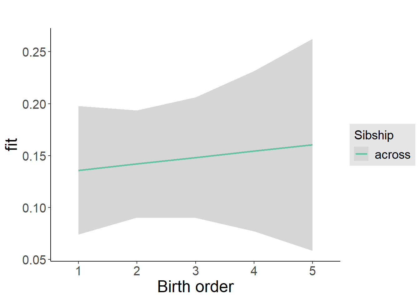
Add Birth Order Factor
Model Summary
m3_birthorder_nonlinear = update(m1_covariates_only, formula = . ~ . + birth_order_nonlinear)
tidy(m3_birthorder_nonlinear, conf.int = T, conf.level = 0.995)| effect | group | term | estimate | std.error | statistic | df | p.value | conf.low | conf.high |
|---|---|---|---|---|---|---|---|---|---|
| fixed | NA | (Intercept) | 0.156 | 0.1934 | 0.8064 | 6926 | 0.4201 | -0.3869 | 0.6988 |
| fixed | NA | poly(age, 3, raw = TRUE)1 | 0.03053 | 0.0186 | 1.641 | 6820 | 0.1008 | -0.02169 | 0.08275 |
| fixed | NA | poly(age, 3, raw = TRUE)2 | -0.001286 | 0.0005446 | -2.361 | 6654 | 0.01824 | -0.002814 | 0.0002427 |
| fixed | NA | poly(age, 3, raw = TRUE)3 | 0.000007278 | 0.000004949 | 1.471 | 6510 | 0.1414 | -0.000006614 | 0.00002117 |
| fixed | NA | male | -0.08019 | 0.02212 | -3.625 | 6900 | 0.000291 | -0.1423 | -0.0181 |
| fixed | NA | sibling_count3 | 0.04936 | 0.03346 | 1.475 | 5316 | 0.1402 | -0.04456 | 0.1433 |
| fixed | NA | sibling_count4 | 0.03168 | 0.03559 | 0.8901 | 5267 | 0.3735 | -0.06823 | 0.1316 |
| fixed | NA | sibling_count5 | -0.00781 | 0.0386 | -0.2023 | 5233 | 0.8397 | -0.1162 | 0.1005 |
| fixed | NA | birth_order_nonlinear2 | 0.02941 | 0.02591 | 1.135 | 5840 | 0.2564 | -0.04332 | 0.1021 |
| fixed | NA | birth_order_nonlinear3 | -0.00886 | 0.03324 | -0.2666 | 5688 | 0.7898 | -0.1022 | 0.08444 |
| fixed | NA | birth_order_nonlinear4 | 0.01245 | 0.04341 | 0.2867 | 5640 | 0.7744 | -0.1094 | 0.1343 |
| fixed | NA | birth_order_nonlinear5 | 0.05994 | 0.06307 | 0.9503 | 5447 | 0.342 | -0.1171 | 0.237 |
| ran_pars | mother_pidlink | sd__(Intercept) | 0.4081 | NA | NA | NA | NA | NA | NA |
| ran_pars | Residual | sd__Observation | 0.8573 | NA | NA | NA | NA | NA | NA |
Coefficient Plot
plot_birthorder(m3_birthorder_nonlinear, separate = FALSE)
Add Interaction
Model Summary
m4_interaction = update(m3_birthorder_nonlinear, formula = . ~ . - birth_order_nonlinear - sibling_count + count_birth_order)
tidy(m4_interaction, conf.int = T, conf.level = 0.995)| effect | group | term | estimate | std.error | statistic | df | p.value | conf.low | conf.high |
|---|---|---|---|---|---|---|---|---|---|
| fixed | NA | (Intercept) | 0.1607 | 0.1938 | 0.8292 | 6927 | 0.407 | -0.3833 | 0.7048 |
| fixed | NA | poly(age, 3, raw = TRUE)1 | 0.03059 | 0.01861 | 1.644 | 6817 | 0.1003 | -0.02164 | 0.08282 |
| fixed | NA | poly(age, 3, raw = TRUE)2 | -0.001282 | 0.0005447 | -2.353 | 6649 | 0.01867 | -0.002811 | 0.0002475 |
| fixed | NA | poly(age, 3, raw = TRUE)3 | 0.00000719 | 0.000004951 | 1.452 | 6501 | 0.1465 | -0.000006708 | 0.00002109 |
| fixed | NA | male | -0.07979 | 0.02213 | -3.606 | 6891 | 0.0003134 | -0.1419 | -0.01767 |
| fixed | NA | count_birth_order2/2 | 0.00907 | 0.04424 | 0.205 | 5888 | 0.8376 | -0.1151 | 0.1333 |
| fixed | NA | count_birth_order1/3 | 0.06095 | 0.04269 | 1.428 | 7081 | 0.1534 | -0.05888 | 0.1808 |
| fixed | NA | count_birth_order2/3 | 0.04536 | 0.04767 | 0.9516 | 7129 | 0.3414 | -0.08844 | 0.1792 |
| fixed | NA | count_birth_order3/3 | 0.02921 | 0.05336 | 0.5474 | 7136 | 0.5841 | -0.1206 | 0.179 |
| fixed | NA | count_birth_order1/4 | 0.0005352 | 0.04871 | 0.01099 | 7129 | 0.9912 | -0.1362 | 0.1373 |
| fixed | NA | count_birth_order2/4 | 0.09781 | 0.05113 | 1.913 | 7138 | 0.05577 | -0.0457 | 0.2413 |
| fixed | NA | count_birth_order3/4 | 0.01087 | 0.05551 | 0.1958 | 7130 | 0.8447 | -0.1449 | 0.1667 |
| fixed | NA | count_birth_order4/4 | 0.01601 | 0.05882 | 0.2722 | 7113 | 0.7855 | -0.1491 | 0.1811 |
| fixed | NA | count_birth_order1/5 | -0.04564 | 0.05519 | -0.8269 | 7137 | 0.4083 | -0.2006 | 0.1093 |
| fixed | NA | count_birth_order2/5 | 0.02042 | 0.05788 | 0.3528 | 7125 | 0.7243 | -0.1421 | 0.1829 |
| fixed | NA | count_birth_order3/5 | -0.01535 | 0.05952 | -0.2579 | 7109 | 0.7965 | -0.1824 | 0.1517 |
| fixed | NA | count_birth_order4/5 | 0.02189 | 0.06302 | 0.3473 | 7077 | 0.7284 | -0.155 | 0.1988 |
| fixed | NA | count_birth_order5/5 | 0.04514 | 0.06441 | 0.7008 | 7065 | 0.4834 | -0.1357 | 0.2259 |
| ran_pars | mother_pidlink | sd__(Intercept) | 0.4088 | NA | NA | NA | NA | NA | NA |
| ran_pars | Residual | sd__Observation | 0.8572 | NA | NA | NA | NA | NA | NA |
Coefficient Plot
plot_birthorder(m4_interaction)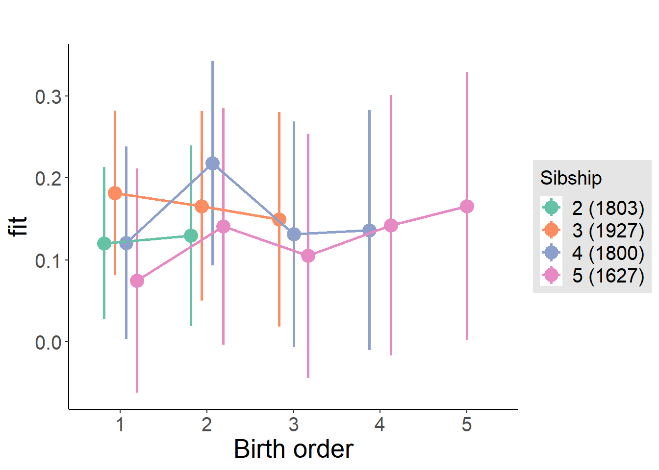
Model Comparison
###### Model 1 - Model 2
anova(m1_covariates_only, m2_birthorder_linear, m3_birthorder_nonlinear, m4_interaction)## refitting model(s) with ML (instead of REML)| Df | AIC | BIC | logLik | deviance | Chisq | Chi Df | Pr(>Chisq) |
|---|---|---|---|---|---|---|---|
| 10 | 19471 | 19540 | -9726 | 19451 | NA | NA | NA |
| 11 | 19473 | 19549 | -9725 | 19451 | 0.3159 | 1 | 0.5741 |
| 14 | 19477 | 19573 | -9724 | 19449 | 2.245 | 3 | 0.5232 |
| 20 | 19485 | 19623 | -9723 | 19445 | 3.571 | 6 | 0.7345 |
Maternal birth order
outcome_uterus_m1 <- update(m2_birthorder_linear, data = birthorder %>%
mutate(sibling_count = sibling_count_uterus_alive_factor,
birth_order_nonlinear = birthorder_uterus_alive_factor,
birth_order = birthorder_uterus_alive,
count_birth_order = count_birthorder_uterus_alive) %>%
filter(sibling_count != "1"))
compare_models_markdown(outcome_uterus_m1)Basic Model
Model Summary
m1_covariates_only <- update(m2_birthorder_linear, formula = . ~ . - birth_order)
tidy(m1_covariates_only, conf.int = T, conf.level = 0.995)| effect | group | term | estimate | std.error | statistic | df | p.value | conf.low | conf.high |
|---|---|---|---|---|---|---|---|---|---|
| fixed | NA | (Intercept) | 0.6686 | 0.5126 | 1.304 | 4500 | 0.1921 | -0.7702 | 2.108 |
| fixed | NA | poly(age, 3, raw = TRUE)1 | -0.03466 | 0.05984 | -0.5792 | 4504 | 0.5625 | -0.2026 | 0.1333 |
| fixed | NA | poly(age, 3, raw = TRUE)2 | 0.00142 | 0.002206 | 0.6438 | 4506 | 0.5198 | -0.004772 | 0.007612 |
| fixed | NA | poly(age, 3, raw = TRUE)3 | -0.0000226 | 0.00002585 | -0.8744 | 4507 | 0.3819 | -0.00009516 | 0.00004996 |
| fixed | NA | male | -0.1245 | 0.02755 | -4.518 | 4415 | 0.000006407 | -0.2018 | -0.04713 |
| fixed | NA | sibling_count3 | 0.02766 | 0.03805 | 0.7269 | 3326 | 0.4673 | -0.07916 | 0.1345 |
| fixed | NA | sibling_count4 | -0.03875 | 0.04118 | -0.9412 | 2935 | 0.3467 | -0.1543 | 0.07683 |
| fixed | NA | sibling_count5 | -0.05762 | 0.04711 | -1.223 | 2635 | 0.2214 | -0.1898 | 0.07462 |
| ran_pars | mother_pidlink | sd__(Intercept) | 0.3611 | NA | NA | NA | NA | NA | NA |
| ran_pars | Residual | sd__Observation | 0.86 | NA | NA | NA | NA | NA | NA |
Coefficient Plot
plot(allEffects(m1_covariates_only, confidence.level = 0.995))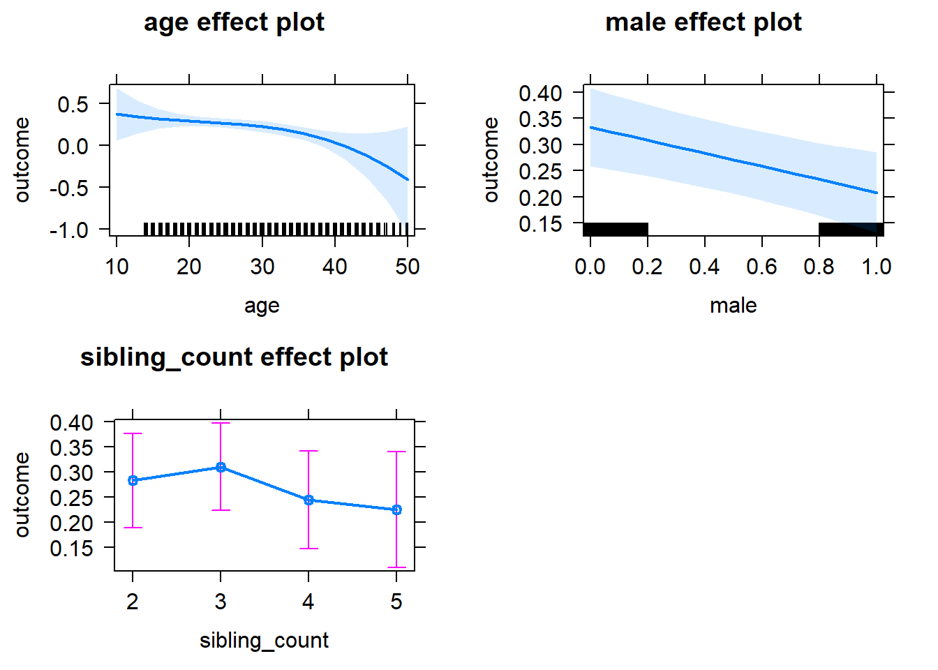
Add Birth Order Linear
Model Summary
tidy(m2_birthorder_linear, conf.int = T, conf.level = 0.995)| effect | group | term | estimate | std.error | statistic | df | p.value | conf.low | conf.high |
|---|---|---|---|---|---|---|---|---|---|
| fixed | NA | (Intercept) | 0.6651 | 0.5133 | 1.296 | 4499 | 0.1951 | -0.7757 | 2.106 |
| fixed | NA | birth_order | 0.002077 | 0.01443 | 0.144 | 4145 | 0.8855 | -0.03841 | 0.04257 |
| fixed | NA | poly(age, 3, raw = TRUE)1 | -0.03453 | 0.05985 | -0.577 | 4503 | 0.564 | -0.2025 | 0.1335 |
| fixed | NA | poly(age, 3, raw = TRUE)2 | 0.001413 | 0.002206 | 0.6405 | 4505 | 0.5219 | -0.00478 | 0.007607 |
| fixed | NA | poly(age, 3, raw = TRUE)3 | -0.00002248 | 0.00002587 | -0.8691 | 4506 | 0.3848 | -0.00009509 | 0.00005013 |
| fixed | NA | male | -0.1245 | 0.02755 | -4.519 | 4414 | 0.000006366 | -0.2019 | -0.04718 |
| fixed | NA | sibling_count3 | 0.02671 | 0.03863 | 0.6914 | 3387 | 0.4894 | -0.08173 | 0.1352 |
| fixed | NA | sibling_count4 | -0.04096 | 0.04394 | -0.9323 | 3159 | 0.3513 | -0.1643 | 0.08237 |
| fixed | NA | sibling_count5 | -0.0613 | 0.05362 | -1.143 | 3143 | 0.253 | -0.2118 | 0.08922 |
| ran_pars | mother_pidlink | sd__(Intercept) | 0.3611 | NA | NA | NA | NA | NA | NA |
| ran_pars | Residual | sd__Observation | 0.8601 | NA | NA | NA | NA | NA | NA |
Coefficient Plot
plot_birthorder2(m2_birthorder_linear, separate = FALSE)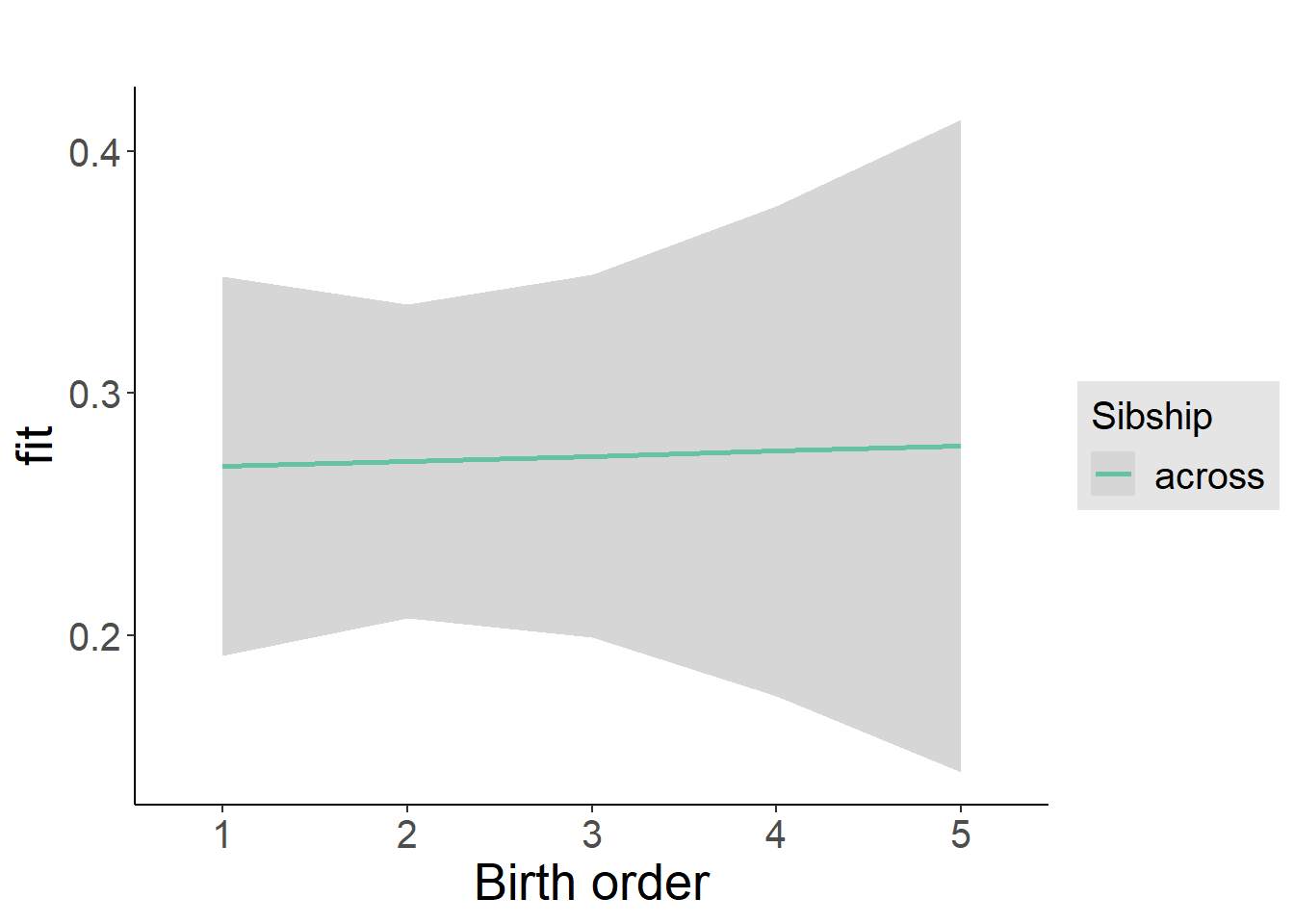
Add Birth Order Factor
Model Summary
m3_birthorder_nonlinear = update(m1_covariates_only, formula = . ~ . + birth_order_nonlinear)
tidy(m3_birthorder_nonlinear, conf.int = T, conf.level = 0.995)| effect | group | term | estimate | std.error | statistic | df | p.value | conf.low | conf.high |
|---|---|---|---|---|---|---|---|---|---|
| fixed | NA | (Intercept) | 0.6623 | 0.5138 | 1.289 | 4500 | 0.1975 | -0.7799 | 2.104 |
| fixed | NA | poly(age, 3, raw = TRUE)1 | -0.03482 | 0.05992 | -0.5812 | 4502 | 0.5612 | -0.203 | 0.1334 |
| fixed | NA | poly(age, 3, raw = TRUE)2 | 0.001424 | 0.002209 | 0.6447 | 4503 | 0.5191 | -0.004776 | 0.007624 |
| fixed | NA | poly(age, 3, raw = TRUE)3 | -0.0000226 | 0.00002589 | -0.8731 | 4503 | 0.3826 | -0.00009528 | 0.00005007 |
| fixed | NA | male | -0.1238 | 0.02756 | -4.493 | 4411 | 0.000007201 | -0.2012 | -0.04647 |
| fixed | NA | sibling_count3 | 0.03289 | 0.0392 | 0.8391 | 3502 | 0.4015 | -0.07715 | 0.1429 |
| fixed | NA | sibling_count4 | -0.02709 | 0.04456 | -0.608 | 3257 | 0.5432 | -0.1522 | 0.09798 |
| fixed | NA | sibling_count5 | -0.06611 | 0.0545 | -1.213 | 3234 | 0.2252 | -0.2191 | 0.08686 |
| fixed | NA | birth_order_nonlinear2 | 0.02273 | 0.0326 | 0.6972 | 3589 | 0.4858 | -0.06878 | 0.1142 |
| fixed | NA | birth_order_nonlinear3 | -0.02193 | 0.0416 | -0.5272 | 3798 | 0.5981 | -0.1387 | 0.09485 |
| fixed | NA | birth_order_nonlinear4 | -0.02637 | 0.05598 | -0.4711 | 3978 | 0.6376 | -0.1835 | 0.1308 |
| fixed | NA | birth_order_nonlinear5 | 0.1112 | 0.0871 | 1.276 | 3829 | 0.2019 | -0.1333 | 0.3557 |
| ran_pars | mother_pidlink | sd__(Intercept) | 0.3602 | NA | NA | NA | NA | NA | NA |
| ran_pars | Residual | sd__Observation | 0.8604 | NA | NA | NA | NA | NA | NA |
Coefficient Plot
plot_birthorder(m3_birthorder_nonlinear, separate = FALSE)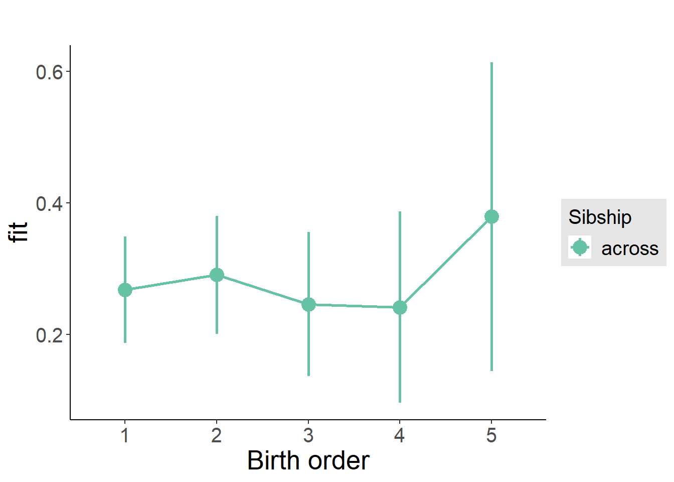
Add Interaction
Model Summary
m4_interaction = update(m3_birthorder_nonlinear, formula = . ~ . - birth_order_nonlinear - sibling_count + count_birth_order)
tidy(m4_interaction, conf.int = T, conf.level = 0.995)| effect | group | term | estimate | std.error | statistic | df | p.value | conf.low | conf.high |
|---|---|---|---|---|---|---|---|---|---|
| fixed | NA | (Intercept) | 0.6748 | 0.514 | 1.313 | 4494 | 0.1894 | -0.7682 | 2.118 |
| fixed | NA | poly(age, 3, raw = TRUE)1 | -0.03349 | 0.05995 | -0.5586 | 4495 | 0.5765 | -0.2018 | 0.1348 |
| fixed | NA | poly(age, 3, raw = TRUE)2 | 0.001357 | 0.00221 | 0.6141 | 4497 | 0.5392 | -0.004847 | 0.007561 |
| fixed | NA | poly(age, 3, raw = TRUE)3 | -0.00002158 | 0.00002591 | -0.8329 | 4497 | 0.405 | -0.00009431 | 0.00005115 |
| fixed | NA | male | -0.1235 | 0.02758 | -4.478 | 4405 | 0.000007728 | -0.2009 | -0.04609 |
| fixed | NA | count_birth_order2/2 | -0.04003 | 0.05604 | -0.7142 | 3808 | 0.4751 | -0.1973 | 0.1173 |
| fixed | NA | count_birth_order1/3 | 0.01968 | 0.04988 | 0.3946 | 4483 | 0.6932 | -0.1203 | 0.1597 |
| fixed | NA | count_birth_order2/3 | 0.03583 | 0.05443 | 0.6583 | 4497 | 0.5104 | -0.117 | 0.1886 |
| fixed | NA | count_birth_order3/3 | -0.02706 | 0.06078 | -0.4452 | 4491 | 0.6562 | -0.1977 | 0.1436 |
| fixed | NA | count_birth_order1/4 | -0.09086 | 0.0612 | -1.485 | 4494 | 0.1377 | -0.2626 | 0.08093 |
| fixed | NA | count_birth_order2/4 | 0.01249 | 0.06311 | 0.1979 | 4495 | 0.8431 | -0.1647 | 0.1896 |
| fixed | NA | count_birth_order3/4 | -0.06358 | 0.06656 | -0.9552 | 4477 | 0.3395 | -0.2504 | 0.1233 |
| fixed | NA | count_birth_order4/4 | -0.06842 | 0.06923 | -0.9883 | 4474 | 0.323 | -0.2628 | 0.1259 |
| fixed | NA | count_birth_order1/5 | -0.132 | 0.08314 | -1.588 | 4489 | 0.1124 | -0.3654 | 0.1014 |
| fixed | NA | count_birth_order2/5 | -0.03475 | 0.08868 | -0.3919 | 4455 | 0.6952 | -0.2837 | 0.2142 |
| fixed | NA | count_birth_order3/5 | -0.08159 | 0.08307 | -0.9822 | 4453 | 0.3261 | -0.3148 | 0.1516 |
| fixed | NA | count_birth_order4/5 | -0.1201 | 0.07999 | -1.501 | 4465 | 0.1335 | -0.3446 | 0.1045 |
| fixed | NA | count_birth_order5/5 | 0.02451 | 0.08316 | 0.2948 | 4448 | 0.7682 | -0.2089 | 0.2579 |
| ran_pars | mother_pidlink | sd__(Intercept) | 0.3594 | NA | NA | NA | NA | NA | NA |
| ran_pars | Residual | sd__Observation | 0.861 | NA | NA | NA | NA | NA | NA |
Coefficient Plot
plot_birthorder(m4_interaction)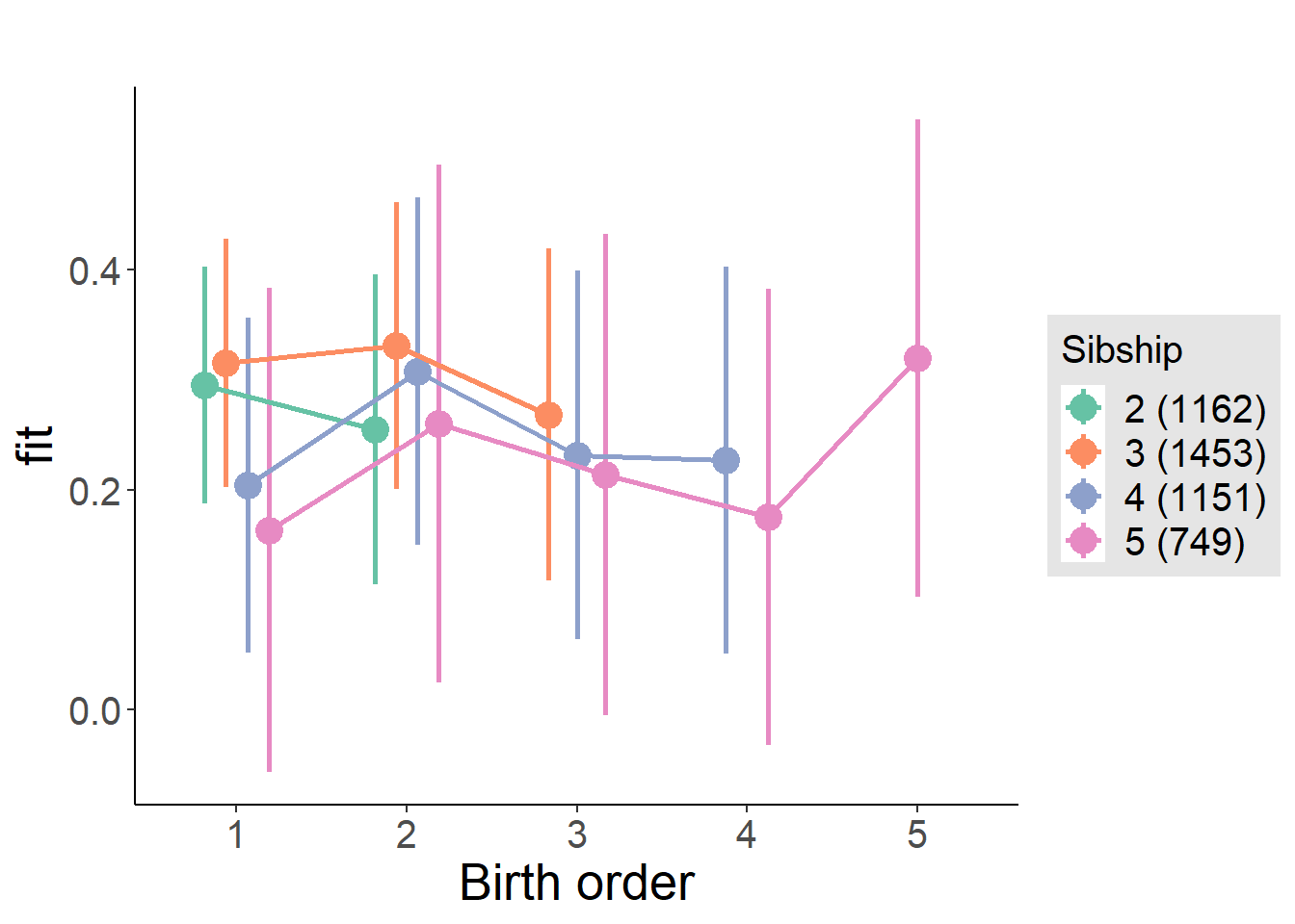
Model Comparison
###### Model 1 - Model 2
anova(m1_covariates_only, m2_birthorder_linear, m3_birthorder_nonlinear, m4_interaction)## refitting model(s) with ML (instead of REML)| Df | AIC | BIC | logLik | deviance | Chisq | Chi Df | Pr(>Chisq) |
|---|---|---|---|---|---|---|---|
| 10 | 12158 | 12222 | -6069 | 12138 | NA | NA | NA |
| 11 | 12160 | 12230 | -6069 | 12138 | 0.02078 | 1 | 0.8854 |
| 14 | 12162 | 12252 | -6067 | 12134 | 3.517 | 3 | 0.3185 |
| 20 | 12171 | 12299 | -6065 | 12131 | 3.434 | 6 | 0.7527 |
Maternal pregnancy order
outcome_preg_m1 <- update(m2_birthorder_linear, data = birthorder %>%
mutate(sibling_count = sibling_count_uterus_preg_factor,
birth_order_nonlinear = birthorder_uterus_preg_factor,
birth_order = birthorder_uterus_preg,
count_birth_order = count_birthorder_uterus_preg
) %>%
filter(sibling_count != "1"))
compare_models_markdown(outcome_preg_m1)Basic Model
Model Summary
m1_covariates_only <- update(m2_birthorder_linear, formula = . ~ . - birth_order)
tidy(m1_covariates_only, conf.int = T, conf.level = 0.995)| effect | group | term | estimate | std.error | statistic | df | p.value | conf.low | conf.high |
|---|---|---|---|---|---|---|---|---|---|
| fixed | NA | (Intercept) | 0.695 | 0.5289 | 1.314 | 4175 | 0.1889 | -0.7896 | 2.18 |
| fixed | NA | poly(age, 3, raw = TRUE)1 | -0.0338 | 0.0618 | -0.5469 | 4179 | 0.5845 | -0.2073 | 0.1397 |
| fixed | NA | poly(age, 3, raw = TRUE)2 | 0.001282 | 0.002279 | 0.5627 | 4182 | 0.5737 | -0.005115 | 0.007679 |
| fixed | NA | poly(age, 3, raw = TRUE)3 | -0.00002026 | 0.00002671 | -0.7584 | 4183 | 0.4483 | -0.00009523 | 0.00005472 |
| fixed | NA | male | -0.1249 | 0.02866 | -4.36 | 4093 | 0.00001334 | -0.2054 | -0.0445 |
| fixed | NA | sibling_count3 | 0.01693 | 0.04122 | 0.4107 | 3177 | 0.6813 | -0.09877 | 0.1326 |
| fixed | NA | sibling_count4 | -0.04111 | 0.04362 | -0.9424 | 2900 | 0.3461 | -0.1636 | 0.08134 |
| fixed | NA | sibling_count5 | -0.0009798 | 0.04684 | -0.02092 | 2611 | 0.9833 | -0.1325 | 0.1305 |
| ran_pars | mother_pidlink | sd__(Intercept) | 0.3614 | NA | NA | NA | NA | NA | NA |
| ran_pars | Residual | sd__Observation | 0.8616 | NA | NA | NA | NA | NA | NA |
Coefficient Plot
plot(allEffects(m1_covariates_only, confidence.level = 0.995))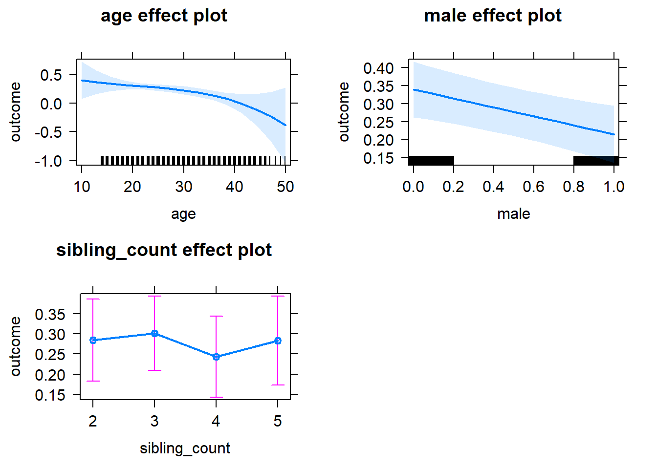
Add Birth Order Linear
Model Summary
tidy(m2_birthorder_linear, conf.int = T, conf.level = 0.995)| effect | group | term | estimate | std.error | statistic | df | p.value | conf.low | conf.high |
|---|---|---|---|---|---|---|---|---|---|
| fixed | NA | (Intercept) | 0.7063 | 0.5295 | 1.334 | 4174 | 0.1823 | -0.7801 | 2.193 |
| fixed | NA | birth_order | -0.006704 | 0.0145 | -0.4624 | 3924 | 0.6438 | -0.04741 | 0.034 |
| fixed | NA | poly(age, 3, raw = TRUE)1 | -0.03414 | 0.06181 | -0.5524 | 4178 | 0.5807 | -0.2076 | 0.1394 |
| fixed | NA | poly(age, 3, raw = TRUE)2 | 0.001301 | 0.002279 | 0.5709 | 4181 | 0.5681 | -0.005097 | 0.0077 |
| fixed | NA | poly(age, 3, raw = TRUE)3 | -0.00002061 | 0.00002672 | -0.7714 | 4182 | 0.4405 | -0.00009563 | 0.0000544 |
| fixed | NA | male | -0.1248 | 0.02866 | -4.354 | 4092 | 0.00001368 | -0.2052 | -0.04434 |
| fixed | NA | sibling_count3 | 0.02 | 0.04176 | 0.4791 | 3219 | 0.6319 | -0.0972 | 0.1372 |
| fixed | NA | sibling_count4 | -0.03424 | 0.04609 | -0.7428 | 3064 | 0.4576 | -0.1636 | 0.09514 |
| fixed | NA | sibling_count5 | 0.01 | 0.05252 | 0.1905 | 2998 | 0.849 | -0.1374 | 0.1574 |
| ran_pars | mother_pidlink | sd__(Intercept) | 0.3614 | NA | NA | NA | NA | NA | NA |
| ran_pars | Residual | sd__Observation | 0.8617 | NA | NA | NA | NA | NA | NA |
Coefficient Plot
plot_birthorder2(m2_birthorder_linear, separate = FALSE)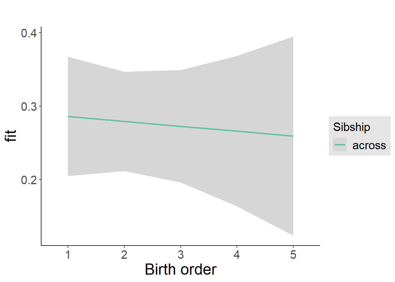
Add Birth Order Factor
Model Summary
m3_birthorder_nonlinear = update(m1_covariates_only, formula = . ~ . + birth_order_nonlinear)
tidy(m3_birthorder_nonlinear, conf.int = T, conf.level = 0.995)| effect | group | term | estimate | std.error | statistic | df | p.value | conf.low | conf.high |
|---|---|---|---|---|---|---|---|---|---|
| fixed | NA | (Intercept) | 0.6616 | 0.53 | 1.248 | 4175 | 0.212 | -0.826 | 2.149 |
| fixed | NA | poly(age, 3, raw = TRUE)1 | -0.03172 | 0.06186 | -0.5128 | 4177 | 0.6081 | -0.2054 | 0.1419 |
| fixed | NA | poly(age, 3, raw = TRUE)2 | 0.001213 | 0.002281 | 0.5319 | 4179 | 0.5948 | -0.005191 | 0.007617 |
| fixed | NA | poly(age, 3, raw = TRUE)3 | -0.00001965 | 0.00002674 | -0.7348 | 4179 | 0.4625 | -0.00009472 | 0.00005542 |
| fixed | NA | male | -0.1238 | 0.02866 | -4.321 | 4088 | 0.00001594 | -0.2043 | -0.04338 |
| fixed | NA | sibling_count3 | 0.02245 | 0.04234 | 0.5303 | 3315 | 0.596 | -0.0964 | 0.1413 |
| fixed | NA | sibling_count4 | -0.02571 | 0.04671 | -0.5505 | 3151 | 0.582 | -0.1568 | 0.1054 |
| fixed | NA | sibling_count5 | 0.01751 | 0.05305 | 0.33 | 3050 | 0.7414 | -0.1314 | 0.1664 |
| fixed | NA | birth_order_nonlinear2 | 0.04513 | 0.03401 | 1.327 | 3391 | 0.1846 | -0.05034 | 0.1406 |
| fixed | NA | birth_order_nonlinear3 | -0.02175 | 0.04309 | -0.5047 | 3594 | 0.6138 | -0.1427 | 0.0992 |
| fixed | NA | birth_order_nonlinear4 | -0.03946 | 0.05712 | -0.6909 | 3739 | 0.4897 | -0.1998 | 0.1209 |
| fixed | NA | birth_order_nonlinear5 | 0.004556 | 0.08364 | 0.05447 | 3619 | 0.9566 | -0.2302 | 0.2393 |
| ran_pars | mother_pidlink | sd__(Intercept) | 0.3617 | NA | NA | NA | NA | NA | NA |
| ran_pars | Residual | sd__Observation | 0.8615 | NA | NA | NA | NA | NA | NA |
Coefficient Plot
plot_birthorder(m3_birthorder_nonlinear, separate = FALSE)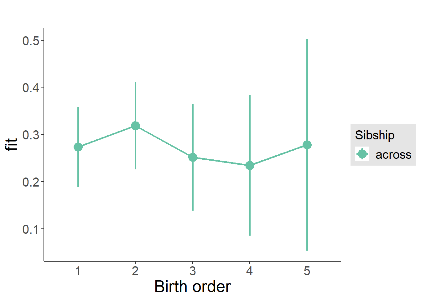
Add Interaction
Model Summary
m4_interaction = update(m3_birthorder_nonlinear, formula = . ~ . - birth_order_nonlinear - sibling_count + count_birth_order)
tidy(m4_interaction, conf.int = T, conf.level = 0.995)| effect | group | term | estimate | std.error | statistic | df | p.value | conf.low | conf.high |
|---|---|---|---|---|---|---|---|---|---|
| fixed | NA | (Intercept) | 0.6742 | 0.5305 | 1.271 | 4169 | 0.2038 | -0.815 | 2.163 |
| fixed | NA | poly(age, 3, raw = TRUE)1 | -0.03249 | 0.06191 | -0.5248 | 4171 | 0.5998 | -0.2063 | 0.1413 |
| fixed | NA | poly(age, 3, raw = TRUE)2 | 0.001232 | 0.002283 | 0.5396 | 4173 | 0.5895 | -0.005178 | 0.007642 |
| fixed | NA | poly(age, 3, raw = TRUE)3 | -0.00001973 | 0.00002677 | -0.737 | 4173 | 0.4612 | -0.00009488 | 0.00005542 |
| fixed | NA | male | -0.1236 | 0.02869 | -4.309 | 4082 | 0.00001678 | -0.2042 | -0.0431 |
| fixed | NA | count_birth_order2/2 | 0.03116 | 0.0615 | 0.5067 | 3585 | 0.6124 | -0.1415 | 0.2038 |
| fixed | NA | count_birth_order1/3 | 0.04129 | 0.05411 | 0.763 | 4161 | 0.4455 | -0.1106 | 0.1932 |
| fixed | NA | count_birth_order2/3 | 0.04748 | 0.05864 | 0.8096 | 4173 | 0.4182 | -0.1171 | 0.2121 |
| fixed | NA | count_birth_order3/3 | -0.029 | 0.06595 | -0.4398 | 4167 | 0.6601 | -0.2141 | 0.1561 |
| fixed | NA | count_birth_order1/4 | -0.08659 | 0.06423 | -1.348 | 4170 | 0.1777 | -0.2669 | 0.09371 |
| fixed | NA | count_birth_order2/4 | 0.04596 | 0.0651 | 0.706 | 4173 | 0.4802 | -0.1368 | 0.2287 |
| fixed | NA | count_birth_order3/4 | -0.02934 | 0.07141 | -0.4108 | 4153 | 0.6812 | -0.2298 | 0.1711 |
| fixed | NA | count_birth_order4/4 | -0.05257 | 0.07366 | -0.7137 | 4153 | 0.4755 | -0.2593 | 0.1542 |
| fixed | NA | count_birth_order1/5 | 0.02131 | 0.07636 | 0.2791 | 4173 | 0.7802 | -0.193 | 0.2357 |
| fixed | NA | count_birth_order2/5 | 0.05541 | 0.0817 | 0.6782 | 4150 | 0.4977 | -0.1739 | 0.2848 |
| fixed | NA | count_birth_order3/5 | 0.001603 | 0.07932 | 0.02021 | 4143 | 0.9839 | -0.2211 | 0.2243 |
| fixed | NA | count_birth_order4/5 | -0.04752 | 0.08212 | -0.5786 | 4125 | 0.5629 | -0.278 | 0.183 |
| fixed | NA | count_birth_order5/5 | 0.01724 | 0.08227 | 0.2095 | 4124 | 0.834 | -0.2137 | 0.2482 |
| ran_pars | mother_pidlink | sd__(Intercept) | 0.3612 | NA | NA | NA | NA | NA | NA |
| ran_pars | Residual | sd__Observation | 0.8621 | NA | NA | NA | NA | NA | NA |
Coefficient Plot
plot_birthorder(m4_interaction)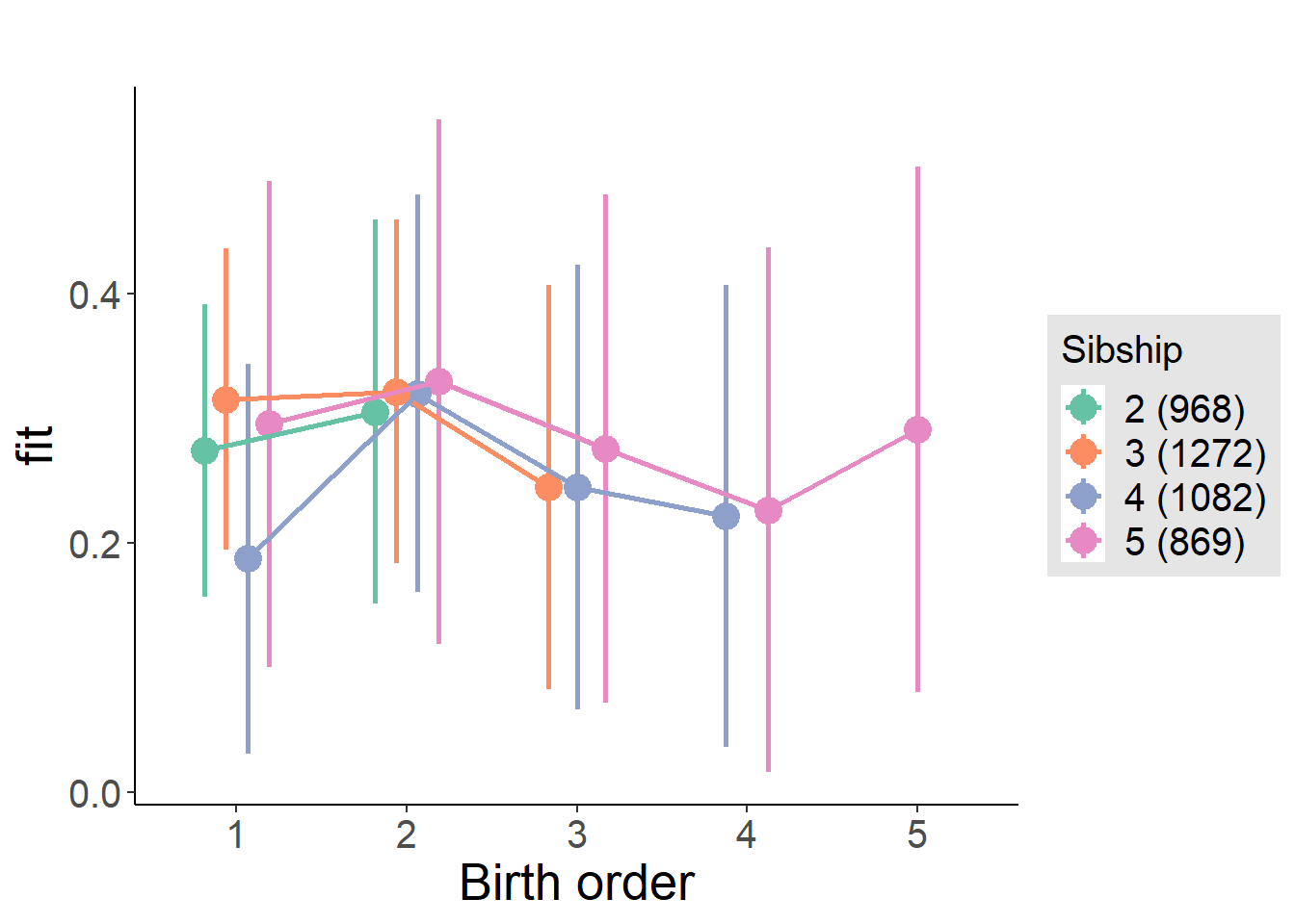
Model Comparison
###### Model 1 - Model 2
anova(m1_covariates_only, m2_birthorder_linear, m3_birthorder_nonlinear, m4_interaction)## refitting model(s) with ML (instead of REML)| Df | AIC | BIC | logLik | deviance | Chisq | Chi Df | Pr(>Chisq) |
|---|---|---|---|---|---|---|---|
| 10 | 11302 | 11365 | -5641 | 11282 | NA | NA | NA |
| 11 | 11303 | 11373 | -5641 | 11281 | 0.2141 | 1 | 0.6436 |
| 14 | 11306 | 11395 | -5639 | 11278 | 3.506 | 3 | 0.32 |
| 20 | 11315 | 11442 | -5638 | 11275 | 2.747 | 6 | 0.8399 |
Parental full sibling order
outcome_parental_m1 <- update(m2_birthorder_linear, data = birthorder %>%
mutate(sibling_count = sibling_count_genes_factor,
birth_order_nonlinear = birthorder_genes_factor,
birth_order = birthorder_genes,
count_birth_order = count_birthorder_genes
) %>%
filter(sibling_count != "1"))
compare_models_markdown(outcome_parental_m1)Basic Model
Model Summary
m1_covariates_only <- update(m2_birthorder_linear, formula = . ~ . - birth_order)
tidy(m1_covariates_only, conf.int = T, conf.level = 0.995)| effect | group | term | estimate | std.error | statistic | df | p.value | conf.low | conf.high |
|---|---|---|---|---|---|---|---|---|---|
| fixed | NA | (Intercept) | 0.5915 | 0.5148 | 1.149 | 4485 | 0.2506 | -0.8534 | 2.036 |
| fixed | NA | poly(age, 3, raw = TRUE)1 | -0.02534 | 0.06017 | -0.4211 | 4489 | 0.6737 | -0.1942 | 0.1436 |
| fixed | NA | poly(age, 3, raw = TRUE)2 | 0.00102 | 0.002221 | 0.4591 | 4491 | 0.6462 | -0.005215 | 0.007255 |
| fixed | NA | poly(age, 3, raw = TRUE)3 | -0.00001703 | 0.00002608 | -0.6529 | 4492 | 0.5139 | -0.00009024 | 0.00005618 |
| fixed | NA | male | -0.1205 | 0.02746 | -4.386 | 4400 | 0.00001179 | -0.1976 | -0.04337 |
| fixed | NA | sibling_count3 | 0.02893 | 0.03739 | 0.7738 | 3307 | 0.4391 | -0.07602 | 0.1339 |
| fixed | NA | sibling_count4 | -0.02826 | 0.04069 | -0.6945 | 2932 | 0.4874 | -0.1425 | 0.08595 |
| fixed | NA | sibling_count5 | -0.04755 | 0.04806 | -0.9894 | 2549 | 0.3226 | -0.1825 | 0.08736 |
| ran_pars | mother_pidlink | sd__(Intercept) | 0.3599 | NA | NA | NA | NA | NA | NA |
| ran_pars | Residual | sd__Observation | 0.8553 | NA | NA | NA | NA | NA | NA |
Coefficient Plot
plot(allEffects(m1_covariates_only, confidence.level = 0.995))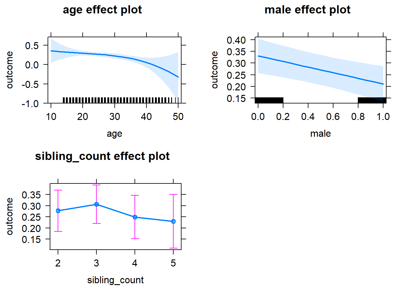
Add Birth Order Linear
Model Summary
tidy(m2_birthorder_linear, conf.int = T, conf.level = 0.995)| effect | group | term | estimate | std.error | statistic | df | p.value | conf.low | conf.high |
|---|---|---|---|---|---|---|---|---|---|
| fixed | NA | (Intercept) | 0.5921 | 0.5154 | 1.149 | 4484 | 0.2507 | -0.8546 | 2.039 |
| fixed | NA | birth_order | -0.0003708 | 0.01454 | -0.0255 | 4110 | 0.9797 | -0.04118 | 0.04044 |
| fixed | NA | poly(age, 3, raw = TRUE)1 | -0.02536 | 0.06018 | -0.4214 | 4488 | 0.6735 | -0.1943 | 0.1436 |
| fixed | NA | poly(age, 3, raw = TRUE)2 | 0.001021 | 0.002222 | 0.4595 | 4490 | 0.6459 | -0.005216 | 0.007258 |
| fixed | NA | poly(age, 3, raw = TRUE)3 | -0.00001705 | 0.0000261 | -0.6533 | 4491 | 0.5136 | -0.00009031 | 0.00005621 |
| fixed | NA | male | -0.1205 | 0.02747 | -4.385 | 4399 | 0.00001186 | -0.1976 | -0.04335 |
| fixed | NA | sibling_count3 | 0.02911 | 0.03799 | 0.7662 | 3364 | 0.4436 | -0.07753 | 0.1357 |
| fixed | NA | sibling_count4 | -0.02787 | 0.0435 | -0.6406 | 3169 | 0.5218 | -0.15 | 0.09424 |
| fixed | NA | sibling_count5 | -0.04692 | 0.05402 | -0.8686 | 3005 | 0.3851 | -0.1986 | 0.1047 |
| ran_pars | mother_pidlink | sd__(Intercept) | 0.3598 | NA | NA | NA | NA | NA | NA |
| ran_pars | Residual | sd__Observation | 0.8555 | NA | NA | NA | NA | NA | NA |
Coefficient Plot
plot_birthorder2(m2_birthorder_linear, separate = FALSE)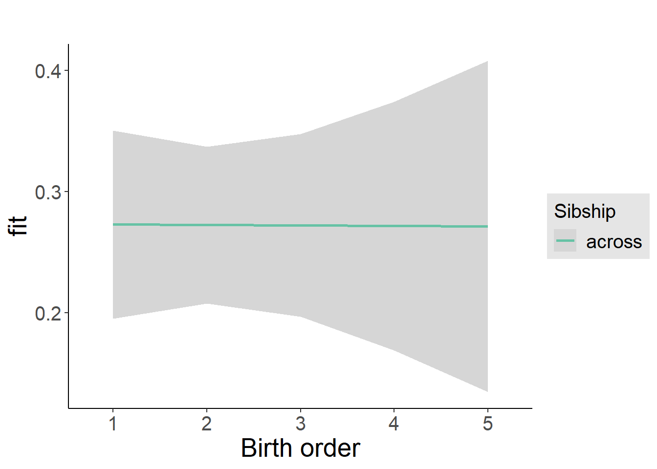
Add Birth Order Factor
Model Summary
m3_birthorder_nonlinear = update(m1_covariates_only, formula = . ~ . + birth_order_nonlinear)
tidy(m3_birthorder_nonlinear, conf.int = T, conf.level = 0.995)| effect | group | term | estimate | std.error | statistic | df | p.value | conf.low | conf.high |
|---|---|---|---|---|---|---|---|---|---|
| fixed | NA | (Intercept) | 0.5839 | 0.516 | 1.132 | 4485 | 0.2578 | -0.8645 | 2.032 |
| fixed | NA | poly(age, 3, raw = TRUE)1 | -0.02524 | 0.06026 | -0.4189 | 4487 | 0.6753 | -0.1944 | 0.1439 |
| fixed | NA | poly(age, 3, raw = TRUE)2 | 0.001018 | 0.002225 | 0.4574 | 4488 | 0.6474 | -0.005227 | 0.007263 |
| fixed | NA | poly(age, 3, raw = TRUE)3 | -0.00001704 | 0.00002613 | -0.6522 | 4488 | 0.5143 | -0.00009037 | 0.0000563 |
| fixed | NA | male | -0.1204 | 0.02748 | -4.38 | 4395 | 0.00001212 | -0.1975 | -0.04324 |
| fixed | NA | sibling_count3 | 0.03159 | 0.03858 | 0.8188 | 3485 | 0.4129 | -0.07671 | 0.1399 |
| fixed | NA | sibling_count4 | -0.01926 | 0.04413 | -0.4365 | 3269 | 0.6625 | -0.1431 | 0.1046 |
| fixed | NA | sibling_count5 | -0.04748 | 0.05509 | -0.8618 | 3107 | 0.3888 | -0.2021 | 0.1072 |
| fixed | NA | birth_order_nonlinear2 | 0.01925 | 0.03225 | 0.5968 | 3569 | 0.5506 | -0.07128 | 0.1098 |
| fixed | NA | birth_order_nonlinear3 | -0.008693 | 0.04126 | -0.2107 | 3758 | 0.8331 | -0.1245 | 0.1071 |
| fixed | NA | birth_order_nonlinear4 | -0.02725 | 0.05691 | -0.4788 | 3941 | 0.6321 | -0.187 | 0.1325 |
| fixed | NA | birth_order_nonlinear5 | 0.05811 | 0.09287 | 0.6257 | 3874 | 0.5315 | -0.2026 | 0.3188 |
| ran_pars | mother_pidlink | sd__(Intercept) | 0.359 | NA | NA | NA | NA | NA | NA |
| ran_pars | Residual | sd__Observation | 0.8559 | NA | NA | NA | NA | NA | NA |
Coefficient Plot
plot_birthorder(m3_birthorder_nonlinear, separate = FALSE)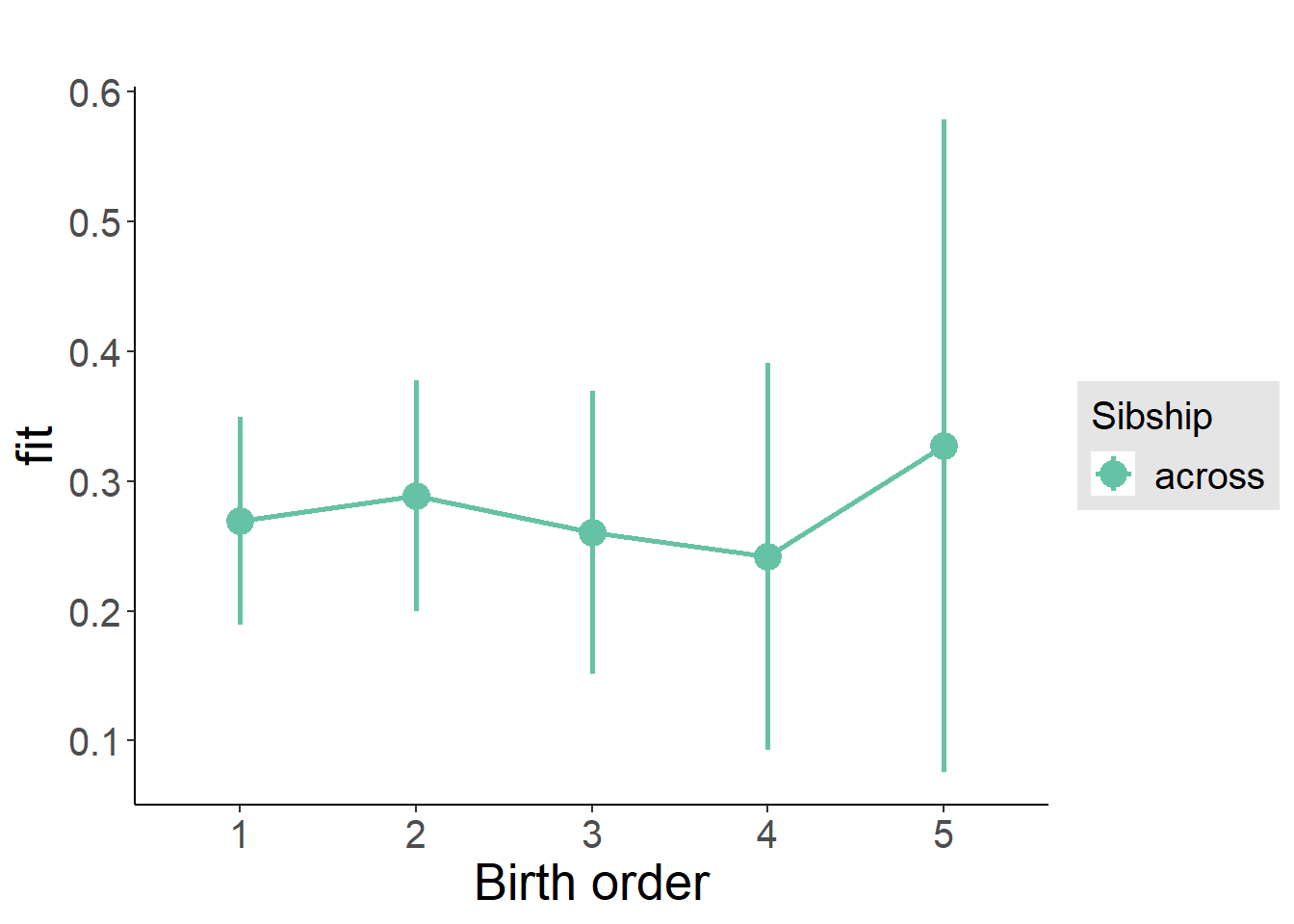
Add Interaction
Model Summary
m4_interaction = update(m3_birthorder_nonlinear, formula = . ~ . - birth_order_nonlinear - sibling_count + count_birth_order)
tidy(m4_interaction, conf.int = T, conf.level = 0.995)| effect | group | term | estimate | std.error | statistic | df | p.value | conf.low | conf.high |
|---|---|---|---|---|---|---|---|---|---|
| fixed | NA | (Intercept) | 0.59 | 0.5164 | 1.142 | 4479 | 0.2533 | -0.8596 | 2.04 |
| fixed | NA | poly(age, 3, raw = TRUE)1 | -0.02401 | 0.06031 | -0.3982 | 4480 | 0.6905 | -0.1933 | 0.1453 |
| fixed | NA | poly(age, 3, raw = TRUE)2 | 0.0009604 | 0.002227 | 0.4313 | 4482 | 0.6662 | -0.00529 | 0.00721 |
| fixed | NA | poly(age, 3, raw = TRUE)3 | -0.00001621 | 0.00002615 | -0.6199 | 4482 | 0.5354 | -0.00008961 | 0.00005719 |
| fixed | NA | male | -0.1201 | 0.0275 | -4.368 | 4389 | 0.00001284 | -0.1973 | -0.04293 |
| fixed | NA | count_birth_order2/2 | -0.02305 | 0.05432 | -0.4244 | 3758 | 0.6713 | -0.1755 | 0.1294 |
| fixed | NA | count_birth_order1/3 | 0.01817 | 0.04906 | 0.3704 | 4466 | 0.7111 | -0.1195 | 0.1559 |
| fixed | NA | count_birth_order2/3 | 0.03697 | 0.05415 | 0.6827 | 4482 | 0.4948 | -0.115 | 0.189 |
| fixed | NA | count_birth_order3/3 | 0.005794 | 0.05943 | 0.0975 | 4474 | 0.9223 | -0.161 | 0.1726 |
| fixed | NA | count_birth_order1/4 | -0.04966 | 0.06118 | -0.8117 | 4481 | 0.417 | -0.2214 | 0.1221 |
| fixed | NA | count_birth_order2/4 | 0.01482 | 0.06269 | 0.2364 | 4479 | 0.8132 | -0.1612 | 0.1908 |
| fixed | NA | count_birth_order3/4 | -0.05328 | 0.06555 | -0.8128 | 4459 | 0.4164 | -0.2373 | 0.1307 |
| fixed | NA | count_birth_order4/4 | -0.064 | 0.06932 | -0.9232 | 4450 | 0.356 | -0.2586 | 0.1306 |
| fixed | NA | count_birth_order1/5 | -0.1075 | 0.08258 | -1.301 | 4479 | 0.1932 | -0.3393 | 0.1243 |
| fixed | NA | count_birth_order2/5 | -0.0238 | 0.09094 | -0.2616 | 4435 | 0.7936 | -0.2791 | 0.2315 |
| fixed | NA | count_birth_order3/5 | -0.0411 | 0.08664 | -0.4743 | 4431 | 0.6353 | -0.2843 | 0.2021 |
| fixed | NA | count_birth_order4/5 | -0.08323 | 0.08347 | -0.9971 | 4446 | 0.3188 | -0.3175 | 0.1511 |
| fixed | NA | count_birth_order5/5 | -0.003306 | 0.0886 | -0.03732 | 4428 | 0.9702 | -0.252 | 0.2454 |
| ran_pars | mother_pidlink | sd__(Intercept) | 0.3584 | NA | NA | NA | NA | NA | NA |
| ran_pars | Residual | sd__Observation | 0.8566 | NA | NA | NA | NA | NA | NA |
Coefficient Plot
plot_birthorder(m4_interaction)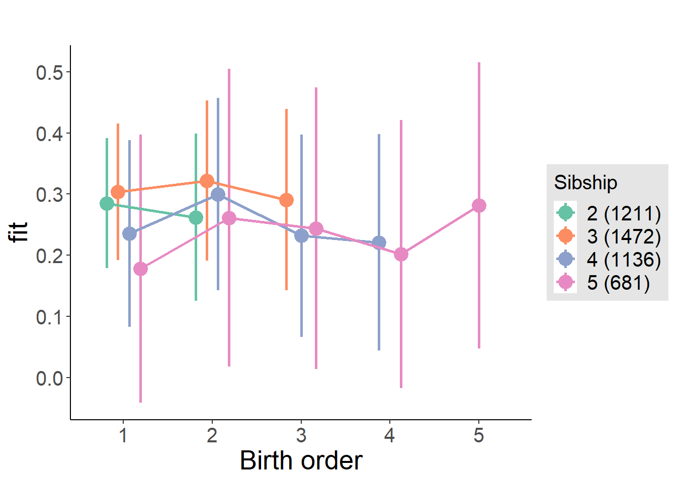
Model Comparison
###### Model 1 - Model 2
anova(m1_covariates_only, m2_birthorder_linear, m3_birthorder_nonlinear, m4_interaction)## refitting model(s) with ML (instead of REML)| Df | AIC | BIC | logLik | deviance | Chisq | Chi Df | Pr(>Chisq) |
|---|---|---|---|---|---|---|---|
| 10 | 12070 | 12135 | -6025 | 12050 | NA | NA | NA |
| 11 | 12072 | 12143 | -6025 | 12050 | 0.0006531 | 1 | 0.9796 |
| 14 | 12077 | 12167 | -6025 | 12049 | 1.409 | 3 | 0.7035 |
| 20 | 12087 | 12216 | -6024 | 12047 | 1.689 | 6 | 0.9459 |
Compare birth order specifications
library(coefplot)
multiplot(outcome_naive_m1, outcome_preg_m1, outcome_uterus_m1, outcome_parental_m1, dodgeHeight = 0.6,
intercept = FALSE)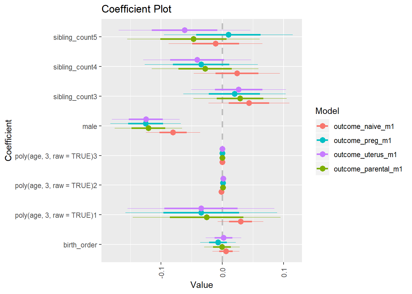
Adaptive Numbering
birthorder <- birthorder %>% mutate(outcome = adaptive_numbering)
model = lmer(outcome ~ birth_order + poly(age, 3, raw = TRUE) + male + sibling_count + (1 | mother_pidlink),
data = birthorder)
compare_birthorder_specs(model)Naive birth order
outcome_naive_m1 <- update(m2_birthorder_linear, data = birthorder %>%
mutate(sibling_count = sibling_count_naive_factor,
birth_order_nonlinear = birthorder_naive_factor,
birth_order = birthorder_naive,
count_birth_order = count_birthorder_naive) %>%
filter(sibling_count != "1"))
compare_models_markdown(outcome_naive_m1)Basic Model
Model Summary
m1_covariates_only <- update(m2_birthorder_linear, formula = . ~ . - birth_order)
tidy(m1_covariates_only, conf.int = T, conf.level = 0.995)| effect | group | term | estimate | std.error | statistic | df | p.value | conf.low | conf.high |
|---|---|---|---|---|---|---|---|---|---|
| fixed | NA | (Intercept) | -0.01499 | 0.1951 | -0.07684 | 7025 | 0.9388 | -0.5626 | 0.5327 |
| fixed | NA | poly(age, 3, raw = TRUE)1 | 0.02448 | 0.0188 | 1.302 | 6960 | 0.193 | -0.0283 | 0.07726 |
| fixed | NA | poly(age, 3, raw = TRUE)2 | -0.000663 | 0.0005511 | -1.203 | 6857 | 0.229 | -0.00221 | 0.000884 |
| fixed | NA | poly(age, 3, raw = TRUE)3 | 0.0000001357 | 0.000005014 | 0.02706 | 6761 | 0.9784 | -0.00001394 | 0.00001421 |
| fixed | NA | male | 0.06532 | 0.0221 | 2.955 | 6727 | 0.003133 | 0.00328 | 0.1274 |
| fixed | NA | sibling_count3 | 0.02239 | 0.03372 | 0.6639 | 4990 | 0.5068 | -0.07227 | 0.117 |
| fixed | NA | sibling_count4 | -0.02749 | 0.03503 | -0.7849 | 4608 | 0.4325 | -0.1258 | 0.07082 |
| fixed | NA | sibling_count5 | -0.001222 | 0.03672 | -0.03328 | 4217 | 0.9735 | -0.1043 | 0.1019 |
| ran_pars | mother_pidlink | sd__(Intercept) | 0.4861 | NA | NA | NA | NA | NA | NA |
| ran_pars | Residual | sd__Observation | 0.8295 | NA | NA | NA | NA | NA | NA |
Coefficient Plot
plot(allEffects(m1_covariates_only, confidence.level = 0.995))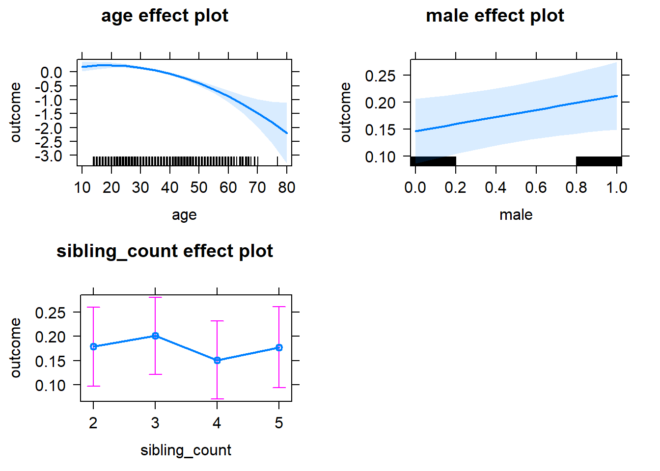
Add Birth Order Linear
Model Summary
tidy(m2_birthorder_linear, conf.int = T, conf.level = 0.995)| effect | group | term | estimate | std.error | statistic | df | p.value | conf.low | conf.high |
|---|---|---|---|---|---|---|---|---|---|
| fixed | NA | (Intercept) | -0.0223 | 0.1952 | -0.1143 | 7013 | 0.909 | -0.5703 | 0.5257 |
| fixed | NA | birth_order | 0.01183 | 0.01081 | 1.095 | 5728 | 0.2738 | -0.01851 | 0.04218 |
| fixed | NA | poly(age, 3, raw = TRUE)1 | 0.02345 | 0.01883 | 1.246 | 6973 | 0.2129 | -0.02939 | 0.07629 |
| fixed | NA | poly(age, 3, raw = TRUE)2 | -0.0006348 | 0.0005517 | -1.151 | 6865 | 0.25 | -0.002183 | 0.0009139 |
| fixed | NA | poly(age, 3, raw = TRUE)3 | -0.00000004854 | 0.000005017 | -0.009675 | 6766 | 0.9923 | -0.00001413 | 0.00001403 |
| fixed | NA | male | 0.06503 | 0.0221 | 2.942 | 6725 | 0.003271 | 0.002985 | 0.1271 |
| fixed | NA | sibling_count3 | 0.01844 | 0.03391 | 0.5437 | 5097 | 0.5867 | -0.07675 | 0.1136 |
| fixed | NA | sibling_count4 | -0.03695 | 0.03608 | -1.024 | 5060 | 0.3057 | -0.1382 | 0.06431 |
| fixed | NA | sibling_count5 | -0.01672 | 0.03936 | -0.4247 | 5128 | 0.671 | -0.1272 | 0.09376 |
| ran_pars | mother_pidlink | sd__(Intercept) | 0.486 | NA | NA | NA | NA | NA | NA |
| ran_pars | Residual | sd__Observation | 0.8295 | NA | NA | NA | NA | NA | NA |
Coefficient Plot
plot_birthorder2(m2_birthorder_linear, separate = FALSE)
Add Birth Order Factor
Model Summary
m3_birthorder_nonlinear = update(m1_covariates_only, formula = . ~ . + birth_order_nonlinear)
tidy(m3_birthorder_nonlinear, conf.int = T, conf.level = 0.995)| effect | group | term | estimate | std.error | statistic | df | p.value | conf.low | conf.high |
|---|---|---|---|---|---|---|---|---|---|
| fixed | NA | (Intercept) | -0.02965 | 0.1956 | -0.1515 | 7021 | 0.8796 | -0.5788 | 0.5195 |
| fixed | NA | poly(age, 3, raw = TRUE)1 | 0.02454 | 0.01884 | 1.303 | 6960 | 0.1927 | -0.02834 | 0.07743 |
| fixed | NA | poly(age, 3, raw = TRUE)2 | -0.0006724 | 0.0005524 | -1.217 | 6840 | 0.2236 | -0.002223 | 0.0008783 |
| fixed | NA | poly(age, 3, raw = TRUE)3 | 0.0000003378 | 0.000005026 | 0.06721 | 6728 | 0.9464 | -0.00001377 | 0.00001445 |
| fixed | NA | male | 0.06497 | 0.0221 | 2.939 | 6722 | 0.0033 | 0.002926 | 0.127 |
| fixed | NA | sibling_count3 | 0.01795 | 0.03434 | 0.5227 | 5273 | 0.6012 | -0.07844 | 0.1143 |
| fixed | NA | sibling_count4 | -0.03119 | 0.03654 | -0.8534 | 5253 | 0.3935 | -0.1338 | 0.07139 |
| fixed | NA | sibling_count5 | -0.01372 | 0.03963 | -0.3461 | 5262 | 0.7293 | -0.125 | 0.09753 |
| fixed | NA | birth_order_nonlinear2 | 0.03908 | 0.02567 | 1.523 | 5696 | 0.1279 | -0.03296 | 0.1111 |
| fixed | NA | birth_order_nonlinear3 | 0.03266 | 0.03286 | 0.9939 | 5484 | 0.3203 | -0.05958 | 0.1249 |
| fixed | NA | birth_order_nonlinear4 | 0.006277 | 0.04289 | 0.1463 | 5402 | 0.8837 | -0.1141 | 0.1267 |
| fixed | NA | birth_order_nonlinear5 | 0.07373 | 0.06223 | 1.185 | 5187 | 0.2361 | -0.1009 | 0.2484 |
| ran_pars | mother_pidlink | sd__(Intercept) | 0.4859 | NA | NA | NA | NA | NA | NA |
| ran_pars | Residual | sd__Observation | 0.8296 | NA | NA | NA | NA | NA | NA |
Coefficient Plot
plot_birthorder(m3_birthorder_nonlinear, separate = FALSE)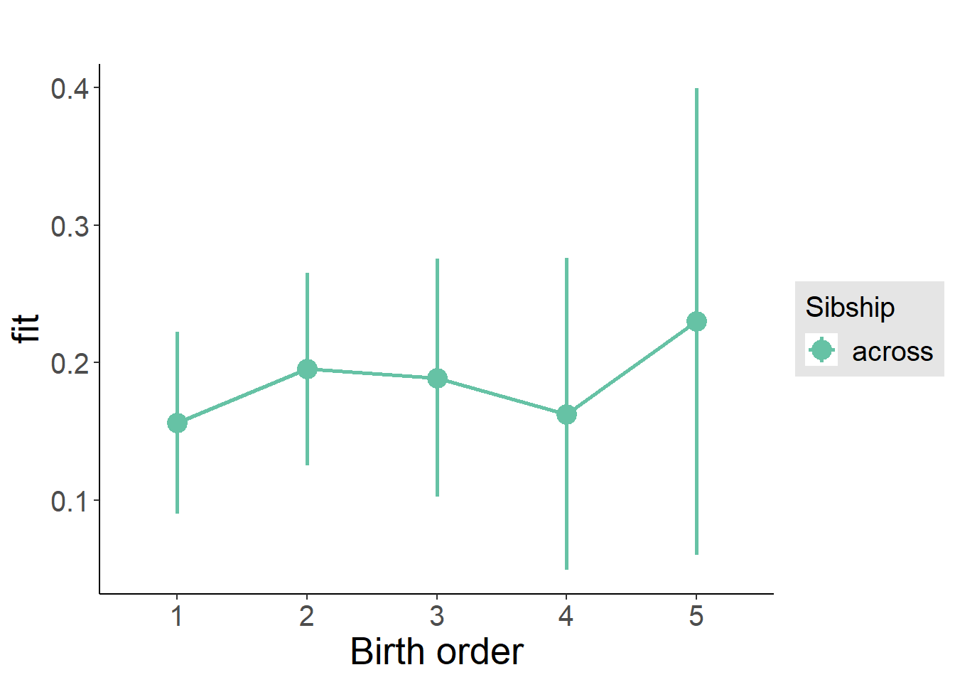
Add Interaction
Model Summary
m4_interaction = update(m3_birthorder_nonlinear, formula = . ~ . - birth_order_nonlinear - sibling_count + count_birth_order)
tidy(m4_interaction, conf.int = T, conf.level = 0.995)| effect | group | term | estimate | std.error | statistic | df | p.value | conf.low | conf.high |
|---|---|---|---|---|---|---|---|---|---|
| fixed | NA | (Intercept) | -0.009529 | 0.196 | -0.04861 | 7018 | 0.9612 | -0.5598 | 0.5407 |
| fixed | NA | poly(age, 3, raw = TRUE)1 | 0.02437 | 0.01884 | 1.293 | 6954 | 0.1959 | -0.02852 | 0.07727 |
| fixed | NA | poly(age, 3, raw = TRUE)2 | -0.0006619 | 0.0005525 | -1.198 | 6832 | 0.231 | -0.002213 | 0.0008891 |
| fixed | NA | poly(age, 3, raw = TRUE)3 | 0.0000001967 | 0.000005028 | 0.03913 | 6716 | 0.9688 | -0.00001392 | 0.00001431 |
| fixed | NA | male | 0.06467 | 0.02211 | 2.925 | 6715 | 0.00346 | 0.002602 | 0.1267 |
| fixed | NA | count_birth_order2/2 | -0.0156 | 0.04384 | -0.3559 | 5813 | 0.7219 | -0.1387 | 0.1075 |
| fixed | NA | count_birth_order1/3 | -0.0183 | 0.04312 | -0.4243 | 7029 | 0.6713 | -0.1393 | 0.1027 |
| fixed | NA | count_birth_order2/3 | 0.05471 | 0.04804 | 1.139 | 7111 | 0.2549 | -0.08015 | 0.1896 |
| fixed | NA | count_birth_order3/3 | 0.04092 | 0.05364 | 0.7627 | 7124 | 0.4456 | -0.1097 | 0.1915 |
| fixed | NA | count_birth_order1/4 | -0.05459 | 0.04907 | -1.112 | 7110 | 0.266 | -0.1923 | 0.08316 |
| fixed | NA | count_birth_order2/4 | -0.02086 | 0.05156 | -0.4046 | 7126 | 0.6858 | -0.1656 | 0.1239 |
| fixed | NA | count_birth_order3/4 | -0.0000896 | 0.05581 | -0.001605 | 7112 | 0.9987 | -0.1568 | 0.1566 |
| fixed | NA | count_birth_order4/4 | -0.04707 | 0.05903 | -0.7973 | 7088 | 0.4253 | -0.2128 | 0.1186 |
| fixed | NA | count_birth_order1/5 | -0.05021 | 0.05549 | -0.9049 | 7127 | 0.3655 | -0.206 | 0.1055 |
| fixed | NA | count_birth_order2/5 | 0.05359 | 0.05826 | 0.9199 | 7108 | 0.3576 | -0.1099 | 0.2171 |
| fixed | NA | count_birth_order3/5 | -0.03637 | 0.05973 | -0.609 | 7084 | 0.5426 | -0.204 | 0.1313 |
| fixed | NA | count_birth_order4/5 | -0.02435 | 0.06318 | -0.3854 | 7034 | 0.6999 | -0.2017 | 0.153 |
| fixed | NA | count_birth_order5/5 | 0.0399 | 0.06455 | 0.6181 | 7019 | 0.5365 | -0.1413 | 0.2211 |
| ran_pars | mother_pidlink | sd__(Intercept) | 0.4855 | NA | NA | NA | NA | NA | NA |
| ran_pars | Residual | sd__Observation | 0.8299 | NA | NA | NA | NA | NA | NA |
Coefficient Plot
plot_birthorder(m4_interaction)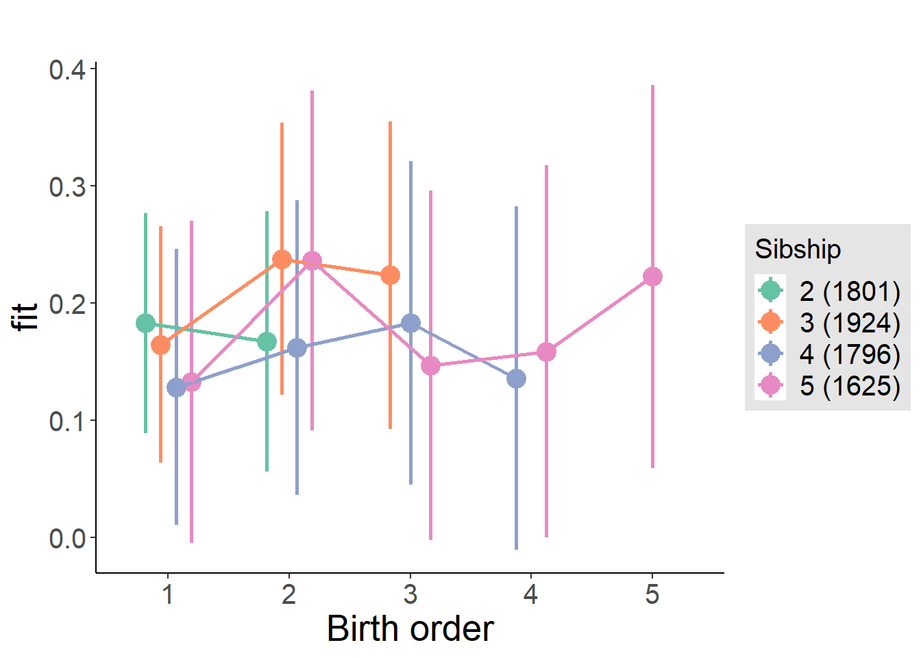
Model Comparison
###### Model 1 - Model 2
anova(m1_covariates_only, m2_birthorder_linear, m3_birthorder_nonlinear, m4_interaction)## refitting model(s) with ML (instead of REML)| Df | AIC | BIC | logLik | deviance | Chisq | Chi Df | Pr(>Chisq) |
|---|---|---|---|---|---|---|---|
| 10 | 19524 | 19592 | -9752 | 19504 | NA | NA | NA |
| 11 | 19525 | 19600 | -9751 | 19503 | 1.199 | 1 | 0.2734 |
| 14 | 19528 | 19624 | -9750 | 19500 | 2.353 | 3 | 0.5024 |
| 20 | 19536 | 19674 | -9748 | 19496 | 4.032 | 6 | 0.6724 |
Maternal birth order
outcome_uterus_m1 <- update(m2_birthorder_linear, data = birthorder %>%
mutate(sibling_count = sibling_count_uterus_alive_factor,
birth_order_nonlinear = birthorder_uterus_alive_factor,
birth_order = birthorder_uterus_alive,
count_birth_order = count_birthorder_uterus_alive) %>%
filter(sibling_count != "1"))
compare_models_markdown(outcome_uterus_m1)Basic Model
Model Summary
m1_covariates_only <- update(m2_birthorder_linear, formula = . ~ . - birth_order)
tidy(m1_covariates_only, conf.int = T, conf.level = 0.995)| effect | group | term | estimate | std.error | statistic | df | p.value | conf.low | conf.high |
|---|---|---|---|---|---|---|---|---|---|
| fixed | NA | (Intercept) | -1.182 | 0.4781 | -2.473 | 4466 | 0.01344 | -2.524 | 0.1598 |
| fixed | NA | poly(age, 3, raw = TRUE)1 | 0.1757 | 0.05583 | 3.146 | 4473 | 0.001665 | 0.01894 | 0.3324 |
| fixed | NA | poly(age, 3, raw = TRUE)2 | -0.006345 | 0.002059 | -3.082 | 4481 | 0.002067 | -0.01212 | -0.0005664 |
| fixed | NA | poly(age, 3, raw = TRUE)3 | 0.00007153 | 0.00002413 | 2.964 | 4487 | 0.003054 | 0.000003785 | 0.0001393 |
| fixed | NA | male | 0.0121 | 0.02561 | 0.4723 | 4311 | 0.6368 | -0.0598 | 0.08399 |
| fixed | NA | sibling_count3 | -0.02085 | 0.03623 | -0.5755 | 3265 | 0.565 | -0.1225 | 0.08084 |
| fixed | NA | sibling_count4 | -0.07205 | 0.03934 | -1.832 | 2928 | 0.06713 | -0.1825 | 0.03838 |
| fixed | NA | sibling_count5 | -0.08284 | 0.04512 | -1.836 | 2679 | 0.06645 | -0.2095 | 0.04381 |
| ran_pars | mother_pidlink | sd__(Intercept) | 0.4106 | NA | NA | NA | NA | NA | NA |
| ran_pars | Residual | sd__Observation | 0.7731 | NA | NA | NA | NA | NA | NA |
Coefficient Plot
plot(allEffects(m1_covariates_only, confidence.level = 0.995))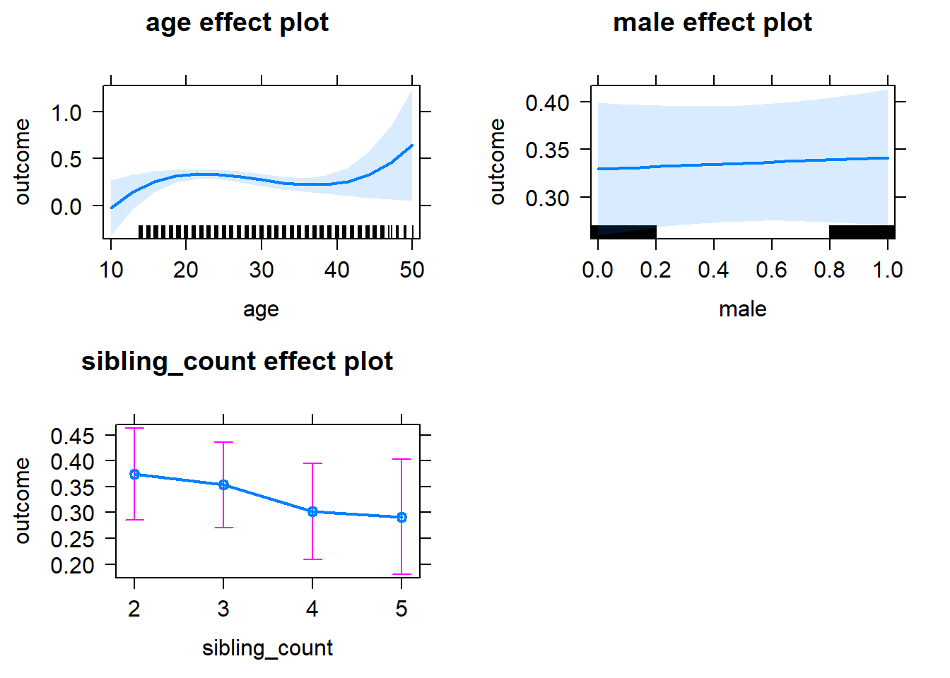
Add Birth Order Linear
Model Summary
tidy(m2_birthorder_linear, conf.int = T, conf.level = 0.995)| effect | group | term | estimate | std.error | statistic | df | p.value | conf.low | conf.high |
|---|---|---|---|---|---|---|---|---|---|
| fixed | NA | (Intercept) | -1.22 | 0.4786 | -2.55 | 4466 | 0.01081 | -2.564 | 0.123 |
| fixed | NA | birth_order | 0.02172 | 0.01335 | 1.627 | 4049 | 0.1038 | -0.01576 | 0.05919 |
| fixed | NA | poly(age, 3, raw = TRUE)1 | 0.1769 | 0.05583 | 3.169 | 4472 | 0.00154 | 0.02021 | 0.3336 |
| fixed | NA | poly(age, 3, raw = TRUE)2 | -0.006412 | 0.002059 | -3.114 | 4480 | 0.001856 | -0.01219 | -0.0006326 |
| fixed | NA | poly(age, 3, raw = TRUE)3 | 0.00007275 | 0.00002414 | 3.014 | 4486 | 0.002595 | 0.000004989 | 0.0001405 |
| fixed | NA | male | 0.0114 | 0.02561 | 0.445 | 4310 | 0.6564 | -0.0605 | 0.08329 |
| fixed | NA | sibling_count3 | -0.03091 | 0.03674 | -0.8411 | 3324 | 0.4004 | -0.134 | 0.07224 |
| fixed | NA | sibling_count4 | -0.09541 | 0.04187 | -2.279 | 3140 | 0.02276 | -0.2129 | 0.02213 |
| fixed | NA | sibling_count5 | -0.1218 | 0.05108 | -2.385 | 3167 | 0.01714 | -0.2652 | 0.02156 |
| ran_pars | mother_pidlink | sd__(Intercept) | 0.4105 | NA | NA | NA | NA | NA | NA |
| ran_pars | Residual | sd__Observation | 0.773 | NA | NA | NA | NA | NA | NA |
Coefficient Plot
plot_birthorder2(m2_birthorder_linear, separate = FALSE)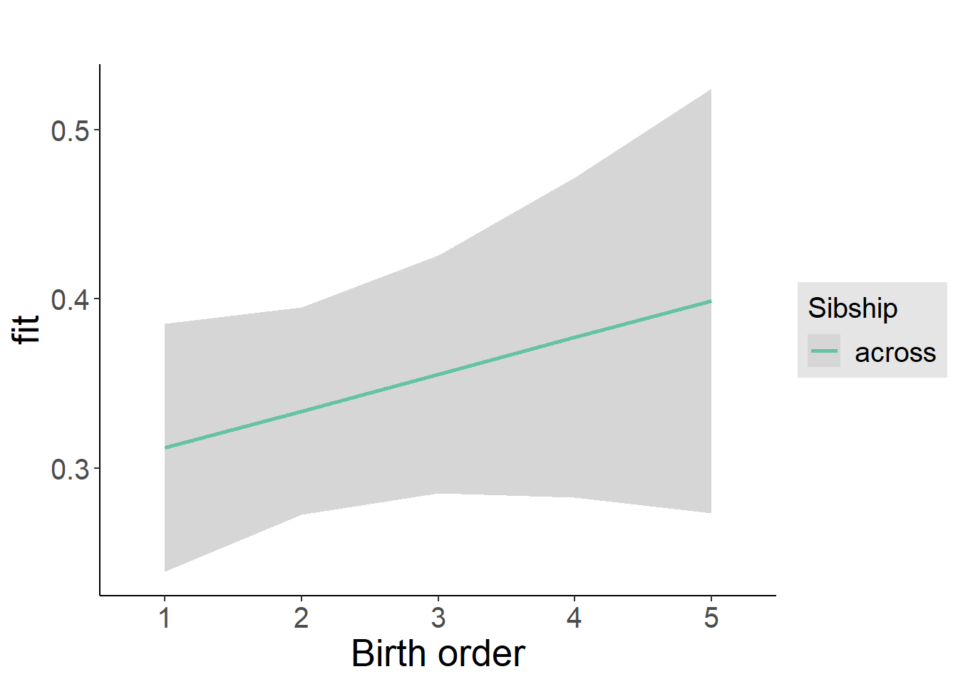
Add Birth Order Factor
Model Summary
m3_birthorder_nonlinear = update(m1_covariates_only, formula = . ~ . + birth_order_nonlinear)
tidy(m3_birthorder_nonlinear, conf.int = T, conf.level = 0.995)| effect | group | term | estimate | std.error | statistic | df | p.value | conf.low | conf.high |
|---|---|---|---|---|---|---|---|---|---|
| fixed | NA | (Intercept) | -1.214 | 0.4794 | -2.532 | 4472 | 0.01136 | -2.56 | 0.1316 |
| fixed | NA | poly(age, 3, raw = TRUE)1 | 0.178 | 0.05592 | 3.184 | 4476 | 0.001465 | 0.02106 | 0.335 |
| fixed | NA | poly(age, 3, raw = TRUE)2 | -0.00645 | 0.002062 | -3.128 | 4482 | 0.001772 | -0.01224 | -0.0006617 |
| fixed | NA | poly(age, 3, raw = TRUE)3 | 0.00007314 | 0.00002417 | 3.026 | 4486 | 0.002495 | 0.000005286 | 0.000141 |
| fixed | NA | male | 0.01198 | 0.02562 | 0.4676 | 4307 | 0.6401 | -0.05995 | 0.08391 |
| fixed | NA | sibling_count3 | -0.03056 | 0.03725 | -0.8204 | 3436 | 0.412 | -0.1351 | 0.07401 |
| fixed | NA | sibling_count4 | -0.08822 | 0.04243 | -2.079 | 3237 | 0.03771 | -0.2073 | 0.0309 |
| fixed | NA | sibling_count5 | -0.1215 | 0.05187 | -2.341 | 3263 | 0.01927 | -0.2671 | 0.02415 |
| fixed | NA | birth_order_nonlinear2 | 0.03861 | 0.03 | 1.287 | 3449 | 0.1981 | -0.0456 | 0.1228 |
| fixed | NA | birth_order_nonlinear3 | 0.04295 | 0.03837 | 1.119 | 3641 | 0.263 | -0.06475 | 0.1507 |
| fixed | NA | birth_order_nonlinear4 | 0.03676 | 0.05169 | 0.7111 | 3832 | 0.477 | -0.1083 | 0.1819 |
| fixed | NA | birth_order_nonlinear5 | 0.1317 | 0.08026 | 1.641 | 3641 | 0.1009 | -0.09359 | 0.357 |
| ran_pars | mother_pidlink | sd__(Intercept) | 0.4103 | NA | NA | NA | NA | NA | NA |
| ran_pars | Residual | sd__Observation | 0.7732 | NA | NA | NA | NA | NA | NA |
Coefficient Plot
plot_birthorder(m3_birthorder_nonlinear, separate = FALSE)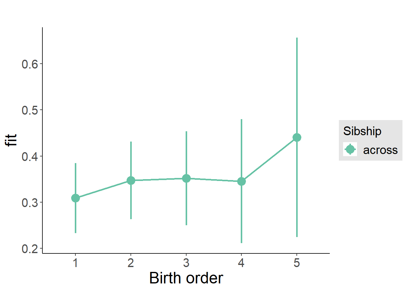
Add Interaction
Model Summary
m4_interaction = update(m3_birthorder_nonlinear, formula = . ~ . - birth_order_nonlinear - sibling_count + count_birth_order)
tidy(m4_interaction, conf.int = T, conf.level = 0.995)| effect | group | term | estimate | std.error | statistic | df | p.value | conf.low | conf.high |
|---|---|---|---|---|---|---|---|---|---|
| fixed | NA | (Intercept) | -1.207 | 0.4796 | -2.517 | 4466 | 0.01187 | -2.553 | 0.1391 |
| fixed | NA | poly(age, 3, raw = TRUE)1 | 0.177 | 0.05594 | 3.164 | 4470 | 0.001565 | 0.01999 | 0.334 |
| fixed | NA | poly(age, 3, raw = TRUE)2 | -0.006382 | 0.002063 | -3.094 | 4475 | 0.00199 | -0.01217 | -0.000591 |
| fixed | NA | poly(age, 3, raw = TRUE)3 | 0.000072 | 0.00002419 | 2.976 | 4480 | 0.002934 | 0.000004093 | 0.0001399 |
| fixed | NA | male | 0.01172 | 0.02564 | 0.457 | 4301 | 0.6477 | -0.06026 | 0.0837 |
| fixed | NA | count_birth_order2/2 | 0.02482 | 0.05171 | 0.48 | 3721 | 0.6312 | -0.1203 | 0.17 |
| fixed | NA | count_birth_order1/3 | -0.05179 | 0.04673 | -1.108 | 4459 | 0.2678 | -0.183 | 0.07939 |
| fixed | NA | count_birth_order2/3 | 0.01877 | 0.05089 | 0.3687 | 4488 | 0.7124 | -0.1241 | 0.1616 |
| fixed | NA | count_birth_order3/3 | 0.01967 | 0.05676 | 0.3466 | 4480 | 0.7289 | -0.1396 | 0.179 |
| fixed | NA | count_birth_order1/4 | -0.1177 | 0.05721 | -2.056 | 4484 | 0.0398 | -0.2782 | 0.04295 |
| fixed | NA | count_birth_order2/4 | -0.05827 | 0.05897 | -0.9881 | 4485 | 0.3231 | -0.2238 | 0.1073 |
| fixed | NA | count_birth_order3/4 | -0.02992 | 0.06212 | -0.4817 | 4455 | 0.63 | -0.2043 | 0.1444 |
| fixed | NA | count_birth_order4/4 | -0.03523 | 0.0645 | -0.5462 | 4451 | 0.5849 | -0.2163 | 0.1458 |
| fixed | NA | count_birth_order1/5 | -0.02122 | 0.07753 | -0.2737 | 4472 | 0.7844 | -0.2388 | 0.1964 |
| fixed | NA | count_birth_order2/5 | -0.107 | 0.08253 | -1.296 | 4405 | 0.1951 | -0.3386 | 0.1247 |
| fixed | NA | count_birth_order3/5 | -0.1429 | 0.07731 | -1.848 | 4408 | 0.06469 | -0.3599 | 0.07415 |
| fixed | NA | count_birth_order4/5 | -0.12 | 0.0745 | -1.611 | 4436 | 0.1073 | -0.3291 | 0.08911 |
| fixed | NA | count_birth_order5/5 | 0.003717 | 0.07739 | 0.04803 | 4409 | 0.9617 | -0.2135 | 0.221 |
| ran_pars | mother_pidlink | sd__(Intercept) | 0.409 | NA | NA | NA | NA | NA | NA |
| ran_pars | Residual | sd__Observation | 0.774 | NA | NA | NA | NA | NA | NA |
Coefficient Plot
plot_birthorder(m4_interaction)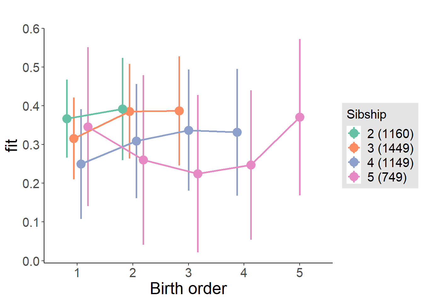
Model Comparison
###### Model 1 - Model 2
anova(m1_covariates_only, m2_birthorder_linear, m3_birthorder_nonlinear, m4_interaction)## refitting model(s) with ML (instead of REML)| Df | AIC | BIC | logLik | deviance | Chisq | Chi Df | Pr(>Chisq) |
|---|---|---|---|---|---|---|---|
| 10 | 11521 | 11585 | -5750 | 11501 | NA | NA | NA |
| 11 | 11520 | 11590 | -5749 | 11498 | 2.651 | 1 | 0.1035 |
| 14 | 11525 | 11614 | -5748 | 11497 | 1.301 | 3 | 0.7289 |
| 20 | 11532 | 11660 | -5746 | 11492 | 4.642 | 6 | 0.5904 |
Maternal pregnancy order
outcome_preg_m1 <- update(m2_birthorder_linear, data = birthorder %>%
mutate(sibling_count = sibling_count_uterus_preg_factor,
birth_order_nonlinear = birthorder_uterus_preg_factor,
birth_order = birthorder_uterus_preg,
count_birth_order = count_birthorder_uterus_preg
) %>%
filter(sibling_count != "1"))
compare_models_markdown(outcome_preg_m1)Basic Model
Model Summary
m1_covariates_only <- update(m2_birthorder_linear, formula = . ~ . - birth_order)
tidy(m1_covariates_only, conf.int = T, conf.level = 0.995)| effect | group | term | estimate | std.error | statistic | df | p.value | conf.low | conf.high |
|---|---|---|---|---|---|---|---|---|---|
| fixed | NA | (Intercept) | -1.383 | 0.4926 | -2.809 | 4138 | 0.004999 | -2.766 | -0.0007621 |
| fixed | NA | poly(age, 3, raw = TRUE)1 | 0.1984 | 0.05757 | 3.446 | 4145 | 0.0005748 | 0.03678 | 0.36 |
| fixed | NA | poly(age, 3, raw = TRUE)2 | -0.007227 | 0.002124 | -3.403 | 4154 | 0.0006723 | -0.01319 | -0.001266 |
| fixed | NA | poly(age, 3, raw = TRUE)3 | 0.00008183 | 0.0000249 | 3.286 | 4161 | 0.001024 | 0.00001193 | 0.0001517 |
| fixed | NA | male | 0.01785 | 0.02658 | 0.6716 | 3981 | 0.5019 | -0.05677 | 0.09248 |
| fixed | NA | sibling_count3 | -0.0001382 | 0.03925 | -0.003522 | 3118 | 0.9972 | -0.1103 | 0.11 |
| fixed | NA | sibling_count4 | -0.04659 | 0.04173 | -1.117 | 2881 | 0.2643 | -0.1637 | 0.07054 |
| fixed | NA | sibling_count5 | -0.03438 | 0.04491 | -0.7656 | 2646 | 0.444 | -0.1604 | 0.09167 |
| ran_pars | mother_pidlink | sd__(Intercept) | 0.4227 | NA | NA | NA | NA | NA | NA |
| ran_pars | Residual | sd__Observation | 0.7681 | NA | NA | NA | NA | NA | NA |
Coefficient Plot
plot(allEffects(m1_covariates_only, confidence.level = 0.995))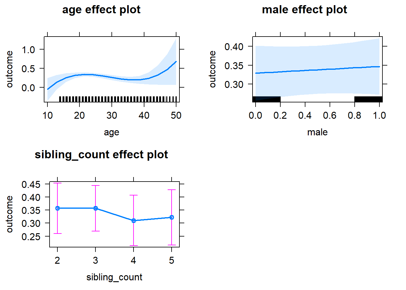
Add Birth Order Linear
Model Summary
tidy(m2_birthorder_linear, conf.int = T, conf.level = 0.995)| effect | group | term | estimate | std.error | statistic | df | p.value | conf.low | conf.high |
|---|---|---|---|---|---|---|---|---|---|
| fixed | NA | (Intercept) | -1.41 | 0.493 | -2.859 | 4137 | 0.004269 | -2.794 | -0.02569 |
| fixed | NA | birth_order | 0.01565 | 0.0134 | 1.168 | 3829 | 0.2429 | -0.02196 | 0.05326 |
| fixed | NA | poly(age, 3, raw = TRUE)1 | 0.1991 | 0.05757 | 3.458 | 4144 | 0.0005498 | 0.03747 | 0.3607 |
| fixed | NA | poly(age, 3, raw = TRUE)2 | -0.007265 | 0.002124 | -3.421 | 4152 | 0.0006303 | -0.01323 | -0.001304 |
| fixed | NA | poly(age, 3, raw = TRUE)3 | 0.00008259 | 0.00002491 | 3.316 | 4159 | 0.000922 | 0.00001267 | 0.0001525 |
| fixed | NA | male | 0.01752 | 0.02658 | 0.6589 | 3980 | 0.51 | -0.05711 | 0.09214 |
| fixed | NA | sibling_count3 | -0.007381 | 0.03974 | -0.1857 | 3160 | 0.8527 | -0.1189 | 0.1042 |
| fixed | NA | sibling_count4 | -0.06285 | 0.04399 | -1.429 | 3036 | 0.1531 | -0.1863 | 0.06062 |
| fixed | NA | sibling_count5 | -0.06031 | 0.05009 | -1.204 | 3012 | 0.2287 | -0.2009 | 0.0803 |
| ran_pars | mother_pidlink | sd__(Intercept) | 0.4228 | NA | NA | NA | NA | NA | NA |
| ran_pars | Residual | sd__Observation | 0.7681 | NA | NA | NA | NA | NA | NA |
Coefficient Plot
plot_birthorder2(m2_birthorder_linear, separate = FALSE)
Add Birth Order Factor
Model Summary
m3_birthorder_nonlinear = update(m1_covariates_only, formula = . ~ . + birth_order_nonlinear)
tidy(m3_birthorder_nonlinear, conf.int = T, conf.level = 0.995)| effect | group | term | estimate | std.error | statistic | df | p.value | conf.low | conf.high |
|---|---|---|---|---|---|---|---|---|---|
| fixed | NA | (Intercept) | -1.401 | 0.4936 | -2.837 | 4146 | 0.00457 | -2.786 | -0.01499 |
| fixed | NA | poly(age, 3, raw = TRUE)1 | 0.1987 | 0.05763 | 3.448 | 4149 | 0.0005709 | 0.03692 | 0.3605 |
| fixed | NA | poly(age, 3, raw = TRUE)2 | -0.007248 | 0.002126 | -3.409 | 4156 | 0.0006572 | -0.01322 | -0.001281 |
| fixed | NA | poly(age, 3, raw = TRUE)3 | 0.00008235 | 0.00002493 | 3.303 | 4161 | 0.0009632 | 0.00001237 | 0.0001523 |
| fixed | NA | male | 0.01819 | 0.02658 | 0.6843 | 3978 | 0.4938 | -0.05643 | 0.0928 |
| fixed | NA | sibling_count3 | -0.002283 | 0.04022 | -0.05675 | 3255 | 0.9547 | -0.1152 | 0.1106 |
| fixed | NA | sibling_count4 | -0.04588 | 0.0445 | -1.031 | 3123 | 0.3027 | -0.1708 | 0.07905 |
| fixed | NA | sibling_count5 | -0.06299 | 0.05053 | -1.247 | 3067 | 0.2126 | -0.2048 | 0.07885 |
| fixed | NA | birth_order_nonlinear2 | 0.04216 | 0.0312 | 1.351 | 3253 | 0.1767 | -0.04542 | 0.1297 |
| fixed | NA | birth_order_nonlinear3 | 0.009415 | 0.03961 | 0.2377 | 3433 | 0.8121 | -0.1018 | 0.1206 |
| fixed | NA | birth_order_nonlinear4 | -0.009049 | 0.0526 | -0.172 | 3587 | 0.8634 | -0.1567 | 0.1386 |
| fixed | NA | birth_order_nonlinear5 | 0.1786 | 0.07685 | 2.324 | 3426 | 0.02021 | -0.03715 | 0.3943 |
| ran_pars | mother_pidlink | sd__(Intercept) | 0.4218 | NA | NA | NA | NA | NA | NA |
| ran_pars | Residual | sd__Observation | 0.7681 | NA | NA | NA | NA | NA | NA |
Coefficient Plot
plot_birthorder(m3_birthorder_nonlinear, separate = FALSE)
Add Interaction
Model Summary
m4_interaction = update(m3_birthorder_nonlinear, formula = . ~ . - birth_order_nonlinear - sibling_count + count_birth_order)
tidy(m4_interaction, conf.int = T, conf.level = 0.995)| effect | group | term | estimate | std.error | statistic | df | p.value | conf.low | conf.high |
|---|---|---|---|---|---|---|---|---|---|
| fixed | NA | (Intercept) | -1.375 | 0.4938 | -2.785 | 4140 | 0.005379 | -2.761 | 0.01094 |
| fixed | NA | poly(age, 3, raw = TRUE)1 | 0.1959 | 0.05764 | 3.399 | 4143 | 0.0006828 | 0.03412 | 0.3577 |
| fixed | NA | poly(age, 3, raw = TRUE)2 | -0.007127 | 0.002127 | -3.352 | 4149 | 0.0008103 | -0.0131 | -0.001158 |
| fixed | NA | poly(age, 3, raw = TRUE)3 | 0.00008071 | 0.00002494 | 3.236 | 4155 | 0.00122 | 0.00001071 | 0.0001507 |
| fixed | NA | male | 0.01721 | 0.02659 | 0.6471 | 3971 | 0.5176 | -0.05744 | 0.09185 |
| fixed | NA | count_birth_order2/2 | 0.0283 | 0.0565 | 0.5009 | 3506 | 0.6165 | -0.1303 | 0.1869 |
| fixed | NA | count_birth_order1/3 | -0.01313 | 0.05059 | -0.2595 | 4138 | 0.7952 | -0.1552 | 0.1289 |
| fixed | NA | count_birth_order2/3 | 0.02001 | 0.0547 | 0.3658 | 4165 | 0.7145 | -0.1335 | 0.1735 |
| fixed | NA | count_birth_order3/3 | 0.03772 | 0.06139 | 0.6144 | 4157 | 0.539 | -0.1346 | 0.21 |
| fixed | NA | count_birth_order1/4 | -0.1026 | 0.05995 | -1.711 | 4161 | 0.0871 | -0.2709 | 0.06569 |
| fixed | NA | count_birth_order2/4 | 0.02987 | 0.06093 | 0.4902 | 4165 | 0.624 | -0.1412 | 0.2009 |
| fixed | NA | count_birth_order3/4 | -0.007508 | 0.06648 | -0.1129 | 4127 | 0.9101 | -0.1941 | 0.1791 |
| fixed | NA | count_birth_order4/4 | -0.06705 | 0.06848 | -0.9791 | 4131 | 0.3276 | -0.2593 | 0.1252 |
| fixed | NA | count_birth_order1/5 | 0.02117 | 0.07115 | 0.2976 | 4164 | 0.766 | -0.1785 | 0.2209 |
| fixed | NA | count_birth_order2/5 | -0.03984 | 0.07592 | -0.5247 | 4114 | 0.5998 | -0.2529 | 0.1733 |
| fixed | NA | count_birth_order3/5 | -0.1577 | 0.07368 | -2.141 | 4107 | 0.03235 | -0.3646 | 0.0491 |
| fixed | NA | count_birth_order4/5 | -0.06692 | 0.07622 | -0.878 | 4080 | 0.38 | -0.2809 | 0.147 |
| fixed | NA | count_birth_order5/5 | 0.1091 | 0.07635 | 1.429 | 4081 | 0.1532 | -0.1052 | 0.3234 |
| ran_pars | mother_pidlink | sd__(Intercept) | 0.4217 | NA | NA | NA | NA | NA | NA |
| ran_pars | Residual | sd__Observation | 0.768 | NA | NA | NA | NA | NA | NA |
Coefficient Plot
plot_birthorder(m4_interaction)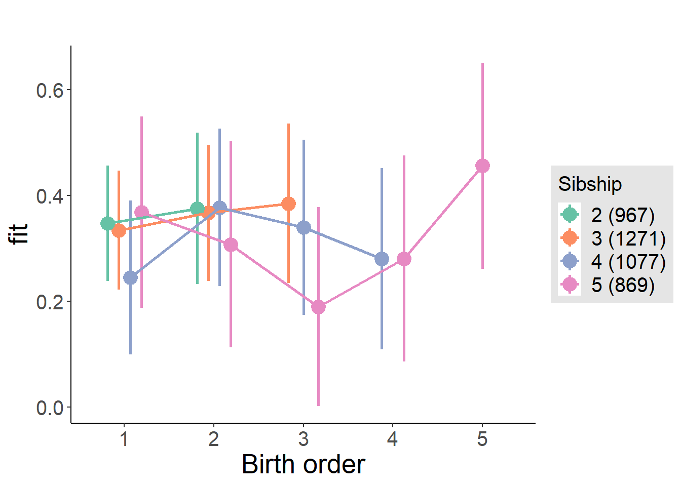
Model Comparison
###### Model 1 - Model 2
anova(m1_covariates_only, m2_birthorder_linear, m3_birthorder_nonlinear, m4_interaction)## refitting model(s) with ML (instead of REML)| Df | AIC | BIC | logLik | deviance | Chisq | Chi Df | Pr(>Chisq) |
|---|---|---|---|---|---|---|---|
| 10 | 10703 | 10766 | -5341 | 10683 | NA | NA | NA |
| 11 | 10703 | 10773 | -5341 | 10681 | 1.367 | 1 | 0.2424 |
| 14 | 10703 | 10792 | -5338 | 10675 | 6.199 | 3 | 0.1023 |
| 20 | 10707 | 10834 | -5333 | 10667 | 8.046 | 6 | 0.2348 |
Parental full sibling order
outcome_parental_m1 <- update(m2_birthorder_linear, data = birthorder %>%
mutate(sibling_count = sibling_count_genes_factor,
birth_order_nonlinear = birthorder_genes_factor,
birth_order = birthorder_genes,
count_birth_order = count_birthorder_genes
) %>%
filter(sibling_count != "1"))
compare_models_markdown(outcome_parental_m1)Basic Model
Model Summary
m1_covariates_only <- update(m2_birthorder_linear, formula = . ~ . - birth_order)
tidy(m1_covariates_only, conf.int = T, conf.level = 0.995)| effect | group | term | estimate | std.error | statistic | df | p.value | conf.low | conf.high |
|---|---|---|---|---|---|---|---|---|---|
| fixed | NA | (Intercept) | -1.192 | 0.4812 | -2.477 | 4446 | 0.0133 | -2.542 | 0.159 |
| fixed | NA | poly(age, 3, raw = TRUE)1 | 0.1748 | 0.05627 | 3.107 | 4454 | 0.001901 | 0.01689 | 0.3328 |
| fixed | NA | poly(age, 3, raw = TRUE)2 | -0.006236 | 0.002078 | -3.001 | 4462 | 0.002704 | -0.01207 | -0.0004034 |
| fixed | NA | poly(age, 3, raw = TRUE)3 | 0.00006911 | 0.00002441 | 2.832 | 4469 | 0.004652 | 0.0000006001 | 0.0001376 |
| fixed | NA | male | 0.006333 | 0.02558 | 0.2476 | 4282 | 0.8045 | -0.06547 | 0.07814 |
| fixed | NA | sibling_count3 | -0.006151 | 0.03575 | -0.172 | 3243 | 0.8634 | -0.1065 | 0.09421 |
| fixed | NA | sibling_count4 | -0.07407 | 0.03906 | -1.897 | 2926 | 0.05798 | -0.1837 | 0.03556 |
| fixed | NA | sibling_count5 | -0.06387 | 0.04631 | -1.379 | 2607 | 0.1679 | -0.1939 | 0.06611 |
| ran_pars | mother_pidlink | sd__(Intercept) | 0.4172 | NA | NA | NA | NA | NA | NA |
| ran_pars | Residual | sd__Observation | 0.7676 | NA | NA | NA | NA | NA | NA |
Coefficient Plot
plot(allEffects(m1_covariates_only, confidence.level = 0.995))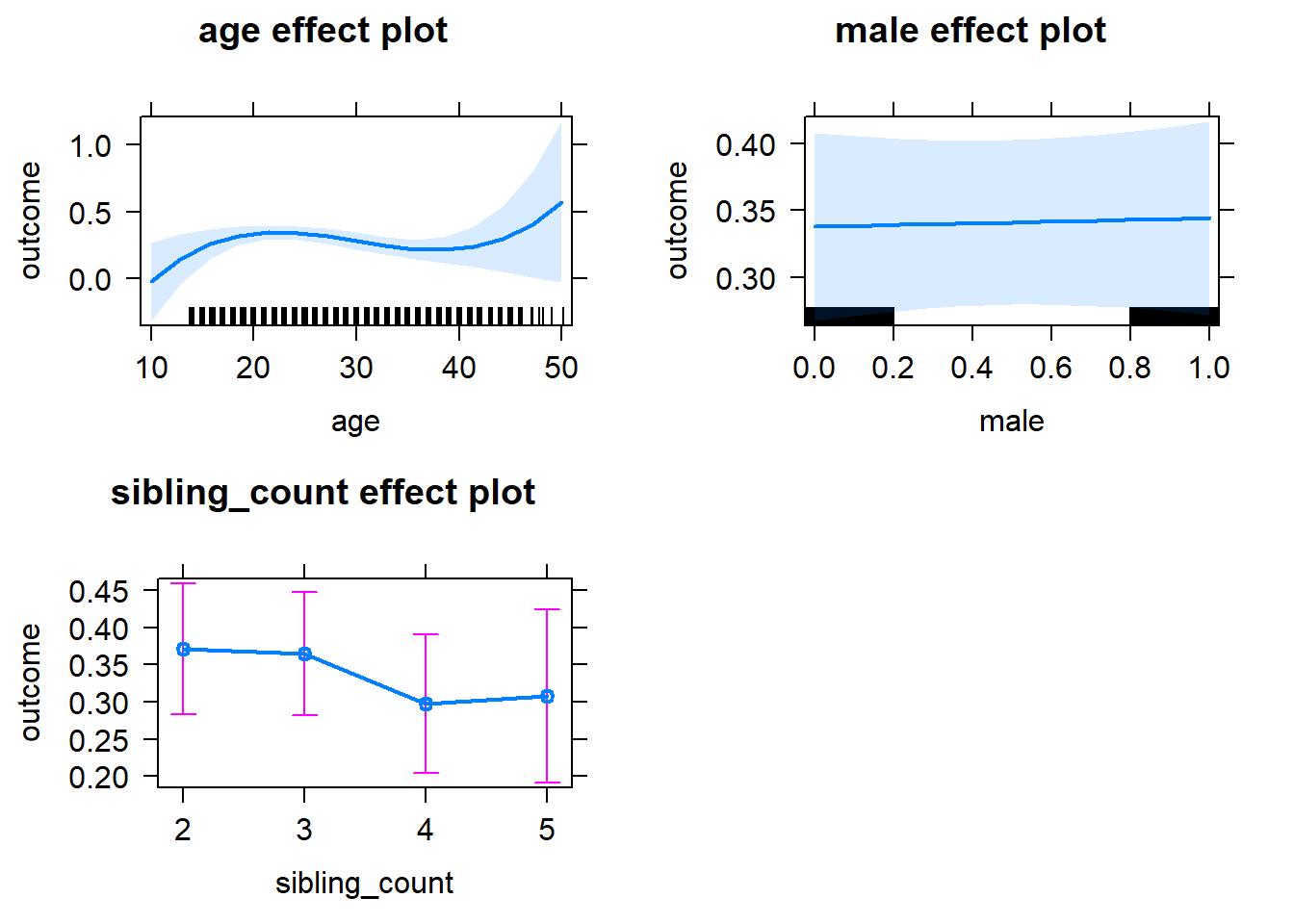
Add Birth Order Linear
Model Summary
tidy(m2_birthorder_linear, conf.int = T, conf.level = 0.995)| effect | group | term | estimate | std.error | statistic | df | p.value | conf.low | conf.high |
|---|---|---|---|---|---|---|---|---|---|
| fixed | NA | (Intercept) | -1.241 | 0.4816 | -2.577 | 4447 | 0.01001 | -2.593 | 0.1109 |
| fixed | NA | birth_order | 0.02818 | 0.01347 | 2.093 | 3996 | 0.03643 | -0.009618 | 0.06599 |
| fixed | NA | poly(age, 3, raw = TRUE)1 | 0.1764 | 0.05625 | 3.136 | 4453 | 0.001726 | 0.01848 | 0.3343 |
| fixed | NA | poly(age, 3, raw = TRUE)2 | -0.006318 | 0.002077 | -3.041 | 4461 | 0.00237 | -0.01215 | -0.0004866 |
| fixed | NA | poly(age, 3, raw = TRUE)3 | 0.00007065 | 0.00002441 | 2.894 | 4468 | 0.003817 | 0.000002133 | 0.0001392 |
| fixed | NA | male | 0.005651 | 0.02557 | 0.221 | 4281 | 0.8251 | -0.06613 | 0.07743 |
| fixed | NA | sibling_count3 | -0.01925 | 0.03628 | -0.5306 | 3298 | 0.5957 | -0.1211 | 0.0826 |
| fixed | NA | sibling_count4 | -0.1043 | 0.04163 | -2.506 | 3151 | 0.01228 | -0.2211 | 0.01255 |
| fixed | NA | sibling_count5 | -0.1123 | 0.05174 | -2.17 | 3042 | 0.03009 | -0.2575 | 0.03297 |
| ran_pars | mother_pidlink | sd__(Intercept) | 0.4169 | NA | NA | NA | NA | NA | NA |
| ran_pars | Residual | sd__Observation | 0.7674 | NA | NA | NA | NA | NA | NA |
Coefficient Plot
plot_birthorder2(m2_birthorder_linear, separate = FALSE)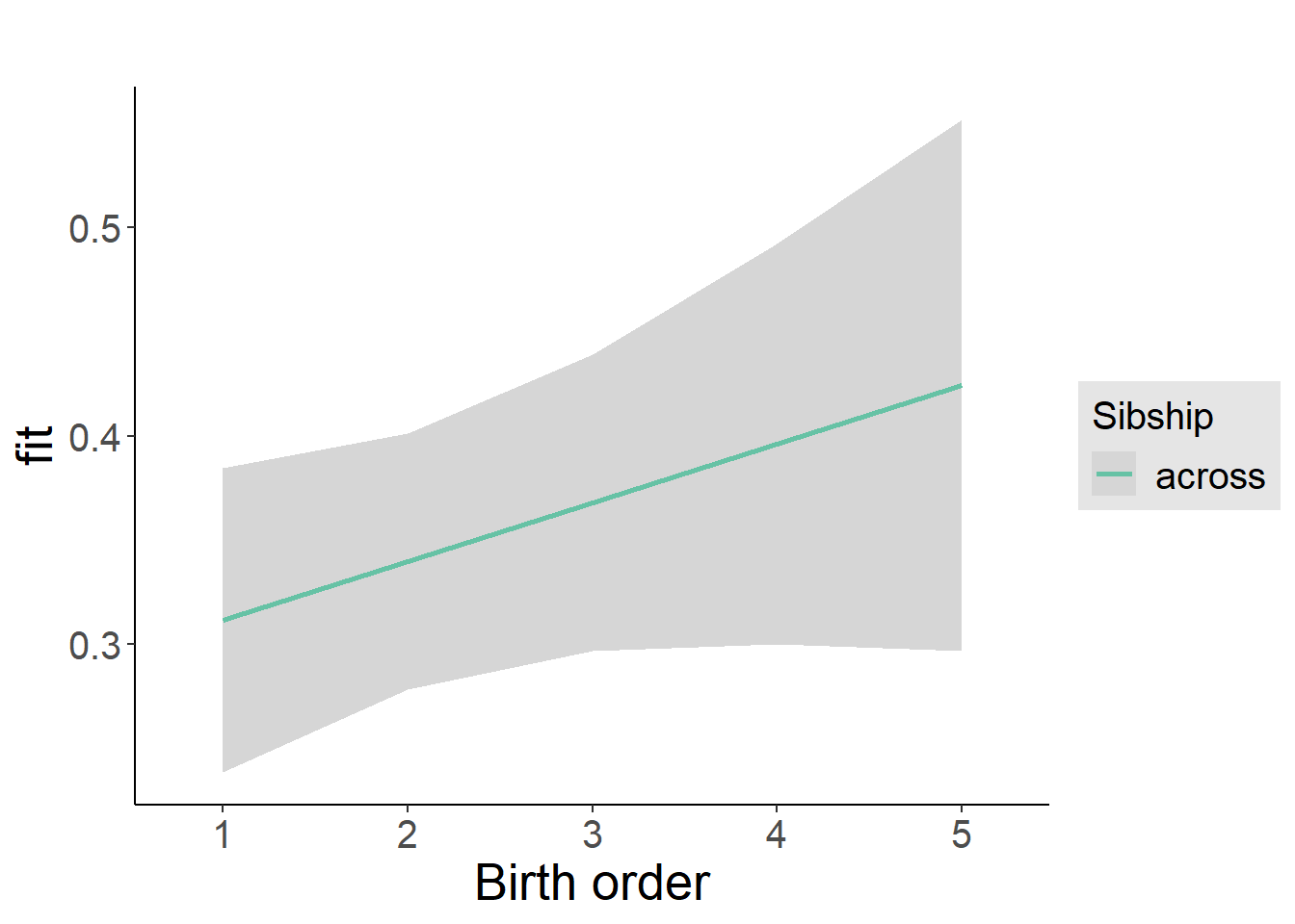
Add Birth Order Factor
Model Summary
m3_birthorder_nonlinear = update(m1_covariates_only, formula = . ~ . + birth_order_nonlinear)
tidy(m3_birthorder_nonlinear, conf.int = T, conf.level = 0.995)| effect | group | term | estimate | std.error | statistic | df | p.value | conf.low | conf.high |
|---|---|---|---|---|---|---|---|---|---|
| fixed | NA | (Intercept) | -1.227 | 0.4824 | -2.543 | 4454 | 0.01101 | -2.581 | 0.1272 |
| fixed | NA | poly(age, 3, raw = TRUE)1 | 0.1771 | 0.05635 | 3.143 | 4458 | 0.001685 | 0.01891 | 0.3352 |
| fixed | NA | poly(age, 3, raw = TRUE)2 | -0.006342 | 0.002081 | -3.048 | 4464 | 0.002317 | -0.01218 | -0.0005015 |
| fixed | NA | poly(age, 3, raw = TRUE)3 | 0.00007089 | 0.00002444 | 2.9 | 4469 | 0.003744 | 0.000002284 | 0.0001395 |
| fixed | NA | male | 0.005679 | 0.02558 | 0.222 | 4277 | 0.8243 | -0.06613 | 0.07749 |
| fixed | NA | sibling_count3 | -0.01592 | 0.03681 | -0.4325 | 3415 | 0.6654 | -0.1192 | 0.0874 |
| fixed | NA | sibling_count4 | -0.09735 | 0.04219 | -2.307 | 3249 | 0.02109 | -0.2158 | 0.02108 |
| fixed | NA | sibling_count5 | -0.1101 | 0.05271 | -2.089 | 3150 | 0.03676 | -0.2581 | 0.03783 |
| fixed | NA | birth_order_nonlinear2 | 0.05219 | 0.02968 | 1.758 | 3404 | 0.07878 | -0.03113 | 0.1355 |
| fixed | NA | birth_order_nonlinear3 | 0.0451 | 0.03806 | 1.185 | 3580 | 0.236 | -0.06172 | 0.1519 |
| fixed | NA | birth_order_nonlinear4 | 0.07206 | 0.05257 | 1.371 | 3766 | 0.1705 | -0.0755 | 0.2196 |
| fixed | NA | birth_order_nonlinear5 | 0.1491 | 0.08566 | 1.74 | 3659 | 0.08196 | -0.09141 | 0.3895 |
| ran_pars | mother_pidlink | sd__(Intercept) | 0.4166 | NA | NA | NA | NA | NA | NA |
| ran_pars | Residual | sd__Observation | 0.7677 | NA | NA | NA | NA | NA | NA |
Coefficient Plot
plot_birthorder(m3_birthorder_nonlinear, separate = FALSE)
Add Interaction
Model Summary
m4_interaction = update(m3_birthorder_nonlinear, formula = . ~ . - birth_order_nonlinear - sibling_count + count_birth_order)
tidy(m4_interaction, conf.int = T, conf.level = 0.995)| effect | group | term | estimate | std.error | statistic | df | p.value | conf.low | conf.high |
|---|---|---|---|---|---|---|---|---|---|
| fixed | NA | (Intercept) | -1.219 | 0.4826 | -2.525 | 4448 | 0.01161 | -2.573 | 0.1362 |
| fixed | NA | poly(age, 3, raw = TRUE)1 | 0.1761 | 0.05637 | 3.124 | 4452 | 0.001799 | 0.01784 | 0.3343 |
| fixed | NA | poly(age, 3, raw = TRUE)2 | -0.006281 | 0.002082 | -3.017 | 4458 | 0.002566 | -0.01212 | -0.0004375 |
| fixed | NA | poly(age, 3, raw = TRUE)3 | 0.00006991 | 0.00002446 | 2.859 | 4463 | 0.004276 | 0.00000126 | 0.0001386 |
| fixed | NA | male | 0.00549 | 0.0256 | 0.2145 | 4271 | 0.8302 | -0.06637 | 0.07735 |
| fixed | NA | count_birth_order2/2 | 0.03835 | 0.05012 | 0.7653 | 3646 | 0.4442 | -0.1023 | 0.179 |
| fixed | NA | count_birth_order1/3 | -0.03473 | 0.04605 | -0.7542 | 4441 | 0.4508 | -0.164 | 0.09454 |
| fixed | NA | count_birth_order2/3 | 0.04904 | 0.05071 | 0.9671 | 4474 | 0.3336 | -0.0933 | 0.1914 |
| fixed | NA | count_birth_order3/3 | 0.02911 | 0.05558 | 0.5237 | 4462 | 0.6005 | -0.1269 | 0.1851 |
| fixed | NA | count_birth_order1/4 | -0.1317 | 0.05728 | -2.3 | 4472 | 0.02149 | -0.2925 | 0.02904 |
| fixed | NA | count_birth_order2/4 | -0.04869 | 0.05866 | -0.83 | 4466 | 0.4066 | -0.2134 | 0.116 |
| fixed | NA | count_birth_order3/4 | -0.03818 | 0.06126 | -0.6233 | 4433 | 0.5331 | -0.2101 | 0.1338 |
| fixed | NA | count_birth_order4/4 | -0.008645 | 0.06466 | -0.1337 | 4419 | 0.8937 | -0.1901 | 0.1729 |
| fixed | NA | count_birth_order1/5 | -0.01297 | 0.07718 | -0.168 | 4464 | 0.8666 | -0.2296 | 0.2037 |
| fixed | NA | count_birth_order2/5 | -0.103 | 0.08474 | -1.216 | 4373 | 0.224 | -0.3409 | 0.1348 |
| fixed | NA | count_birth_order3/5 | -0.1175 | 0.08073 | -1.455 | 4375 | 0.1458 | -0.3441 | 0.1092 |
| fixed | NA | count_birth_order4/5 | -0.07706 | 0.07783 | -0.9902 | 4409 | 0.3221 | -0.2955 | 0.1414 |
| fixed | NA | count_birth_order5/5 | 0.03252 | 0.08254 | 0.394 | 4377 | 0.6936 | -0.1992 | 0.2642 |
| ran_pars | mother_pidlink | sd__(Intercept) | 0.4152 | NA | NA | NA | NA | NA | NA |
| ran_pars | Residual | sd__Observation | 0.7685 | NA | NA | NA | NA | NA | NA |
Coefficient Plot
plot_birthorder(m4_interaction)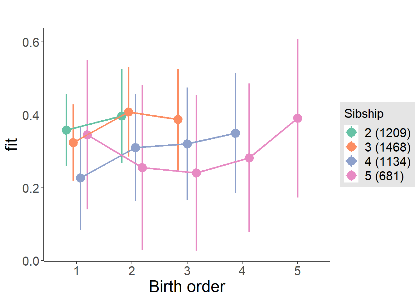
Model Comparison
###### Model 1 - Model 2
anova(m1_covariates_only, m2_birthorder_linear, m3_birthorder_nonlinear, m4_interaction)## refitting model(s) with ML (instead of REML)| Df | AIC | BIC | logLik | deviance | Chisq | Chi Df | Pr(>Chisq) |
|---|---|---|---|---|---|---|---|
| 10 | 11457 | 11522 | -5719 | 11437 | NA | NA | NA |
| 11 | 11455 | 11526 | -5717 | 11433 | 4.387 | 1 | 0.03622 |
| 14 | 11460 | 11549 | -5716 | 11432 | 1.37 | 3 | 0.7125 |
| 20 | 11467 | 11595 | -5714 | 11427 | 4.496 | 6 | 0.6099 |
Compare birth order specifications
library(coefplot)
multiplot(outcome_naive_m1, outcome_preg_m1, outcome_uterus_m1, outcome_parental_m1, dodgeHeight = 0.6,
intercept = FALSE)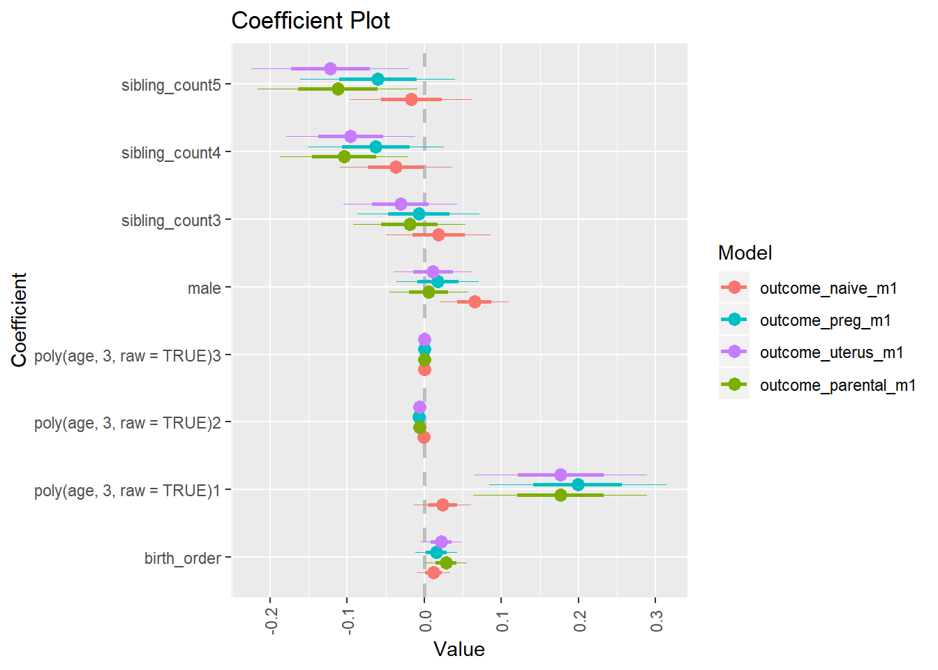
Personality
Extraversion
birthorder <- birthorder %>% mutate(outcome = big5_ext)
model = lmer(outcome ~ birth_order + poly(age, 3, raw = TRUE) + male + sibling_count + (1 | mother_pidlink),
data = birthorder)
compare_birthorder_specs(model)Naive birth order
outcome_naive_m1 <- update(m2_birthorder_linear, data = birthorder %>%
mutate(sibling_count = sibling_count_naive_factor,
birth_order_nonlinear = birthorder_naive_factor,
birth_order = birthorder_naive,
count_birth_order = count_birthorder_naive) %>%
filter(sibling_count != "1"))
compare_models_markdown(outcome_naive_m1)Basic Model
Model Summary
m1_covariates_only <- update(m2_birthorder_linear, formula = . ~ . - birth_order)
tidy(m1_covariates_only, conf.int = T, conf.level = 0.995)| effect | group | term | estimate | std.error | statistic | df | p.value | conf.low | conf.high |
|---|---|---|---|---|---|---|---|---|---|
| fixed | NA | (Intercept) | 0.476 | 0.2004 | 2.375 | 6635 | 0.01759 | -0.08663 | 1.039 |
| fixed | NA | poly(age, 3, raw = TRUE)1 | -0.02873 | 0.01923 | -1.494 | 6434 | 0.1352 | -0.08272 | 0.02525 |
| fixed | NA | poly(age, 3, raw = TRUE)2 | 0.0008189 | 0.0005611 | 1.459 | 6220 | 0.1445 | -0.0007561 | 0.002394 |
| fixed | NA | poly(age, 3, raw = TRUE)3 | -0.000008385 | 0.000005087 | -1.648 | 6062 | 0.09933 | -0.00002266 | 0.000005894 |
| fixed | NA | male | -0.2425 | 0.02352 | -10.31 | 7104 | 9.543e-25 | -0.3085 | -0.1764 |
| fixed | NA | sibling_count3 | 0.006154 | 0.03316 | 0.1856 | 5038 | 0.8528 | -0.08694 | 0.09924 |
| fixed | NA | sibling_count4 | -0.0243 | 0.03408 | -0.713 | 4415 | 0.4759 | -0.12 | 0.07136 |
| fixed | NA | sibling_count5 | -0.03191 | 0.03531 | -0.9037 | 3753 | 0.3662 | -0.131 | 0.06721 |
| ran_pars | mother_pidlink | sd__(Intercept) | 0.215 | NA | NA | NA | NA | NA | NA |
| ran_pars | Residual | sd__Observation | 0.9699 | NA | NA | NA | NA | NA | NA |
Coefficient Plot
plot(allEffects(m1_covariates_only, confidence.level = 0.995))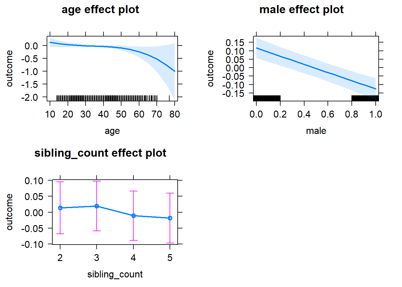
Add Birth Order Linear
Model Summary
tidy(m2_birthorder_linear, conf.int = T, conf.level = 0.995)| effect | group | term | estimate | std.error | statistic | df | p.value | conf.low | conf.high |
|---|---|---|---|---|---|---|---|---|---|
| fixed | NA | (Intercept) | 0.4758 | 0.2005 | 2.373 | 6626 | 0.01765 | -0.08693 | 1.038 |
| fixed | NA | birth_order | 0.0004919 | 0.01182 | 0.0416 | 6238 | 0.9668 | -0.0327 | 0.03368 |
| fixed | NA | poly(age, 3, raw = TRUE)1 | -0.02878 | 0.01927 | -1.494 | 6462 | 0.1354 | -0.08287 | 0.02531 |
| fixed | NA | poly(age, 3, raw = TRUE)2 | 0.0008201 | 0.0005619 | 1.459 | 6235 | 0.1445 | -0.0007572 | 0.002397 |
| fixed | NA | poly(age, 3, raw = TRUE)3 | -0.000008392 | 0.000005091 | -1.649 | 6070 | 0.09929 | -0.00002268 | 0.000005897 |
| fixed | NA | male | -0.2425 | 0.02352 | -10.31 | 7102 | 9.67e-25 | -0.3085 | -0.1764 |
| fixed | NA | sibling_count3 | 0.005976 | 0.03344 | 0.1787 | 5174 | 0.8582 | -0.08789 | 0.09984 |
| fixed | NA | sibling_count4 | -0.02471 | 0.03549 | -0.6962 | 4993 | 0.4863 | -0.1243 | 0.07492 |
| fixed | NA | sibling_count5 | -0.03257 | 0.03873 | -0.8409 | 4912 | 0.4005 | -0.1413 | 0.07616 |
| ran_pars | mother_pidlink | sd__(Intercept) | 0.2149 | NA | NA | NA | NA | NA | NA |
| ran_pars | Residual | sd__Observation | 0.97 | NA | NA | NA | NA | NA | NA |
Coefficient Plot
plot_birthorder2(m2_birthorder_linear, separate = FALSE)
Add Birth Order Factor
Model Summary
m3_birthorder_nonlinear = update(m1_covariates_only, formula = . ~ . + birth_order_nonlinear)
tidy(m3_birthorder_nonlinear, conf.int = T, conf.level = 0.995)| effect | group | term | estimate | std.error | statistic | df | p.value | conf.low | conf.high |
|---|---|---|---|---|---|---|---|---|---|
| fixed | NA | (Intercept) | 0.4474 | 0.201 | 2.226 | 6653 | 0.02608 | -0.1169 | 1.012 |
| fixed | NA | poly(age, 3, raw = TRUE)1 | -0.02775 | 0.01928 | -1.439 | 6451 | 0.1501 | -0.08186 | 0.02636 |
| fixed | NA | poly(age, 3, raw = TRUE)2 | 0.0007794 | 0.0005623 | 1.386 | 6215 | 0.1658 | -0.0007989 | 0.002358 |
| fixed | NA | poly(age, 3, raw = TRUE)3 | -0.000007944 | 0.000005096 | -1.559 | 6039 | 0.119 | -0.00002225 | 0.00000636 |
| fixed | NA | male | -0.2425 | 0.02352 | -10.31 | 7098 | 9.31e-25 | -0.3085 | -0.1765 |
| fixed | NA | sibling_count3 | 0.01114 | 0.03401 | 0.3277 | 5397 | 0.7431 | -0.08431 | 0.1066 |
| fixed | NA | sibling_count4 | -0.01998 | 0.03613 | -0.5532 | 5249 | 0.5802 | -0.1214 | 0.08143 |
| fixed | NA | sibling_count5 | -0.01999 | 0.03914 | -0.5107 | 5099 | 0.6096 | -0.1299 | 0.08988 |
| fixed | NA | birth_order_nonlinear2 | 0.0591 | 0.02811 | 2.103 | 6066 | 0.03554 | -0.0198 | 0.138 |
| fixed | NA | birth_order_nonlinear3 | -0.006697 | 0.03608 | -0.1856 | 6075 | 0.8527 | -0.108 | 0.09457 |
| fixed | NA | birth_order_nonlinear4 | 0.01674 | 0.04711 | 0.3554 | 6112 | 0.7223 | -0.1155 | 0.149 |
| fixed | NA | birth_order_nonlinear5 | -0.02431 | 0.06859 | -0.3544 | 6026 | 0.7231 | -0.2168 | 0.1682 |
| ran_pars | mother_pidlink | sd__(Intercept) | 0.2171 | NA | NA | NA | NA | NA | NA |
| ran_pars | Residual | sd__Observation | 0.9693 | NA | NA | NA | NA | NA | NA |
Coefficient Plot
plot_birthorder(m3_birthorder_nonlinear, separate = FALSE)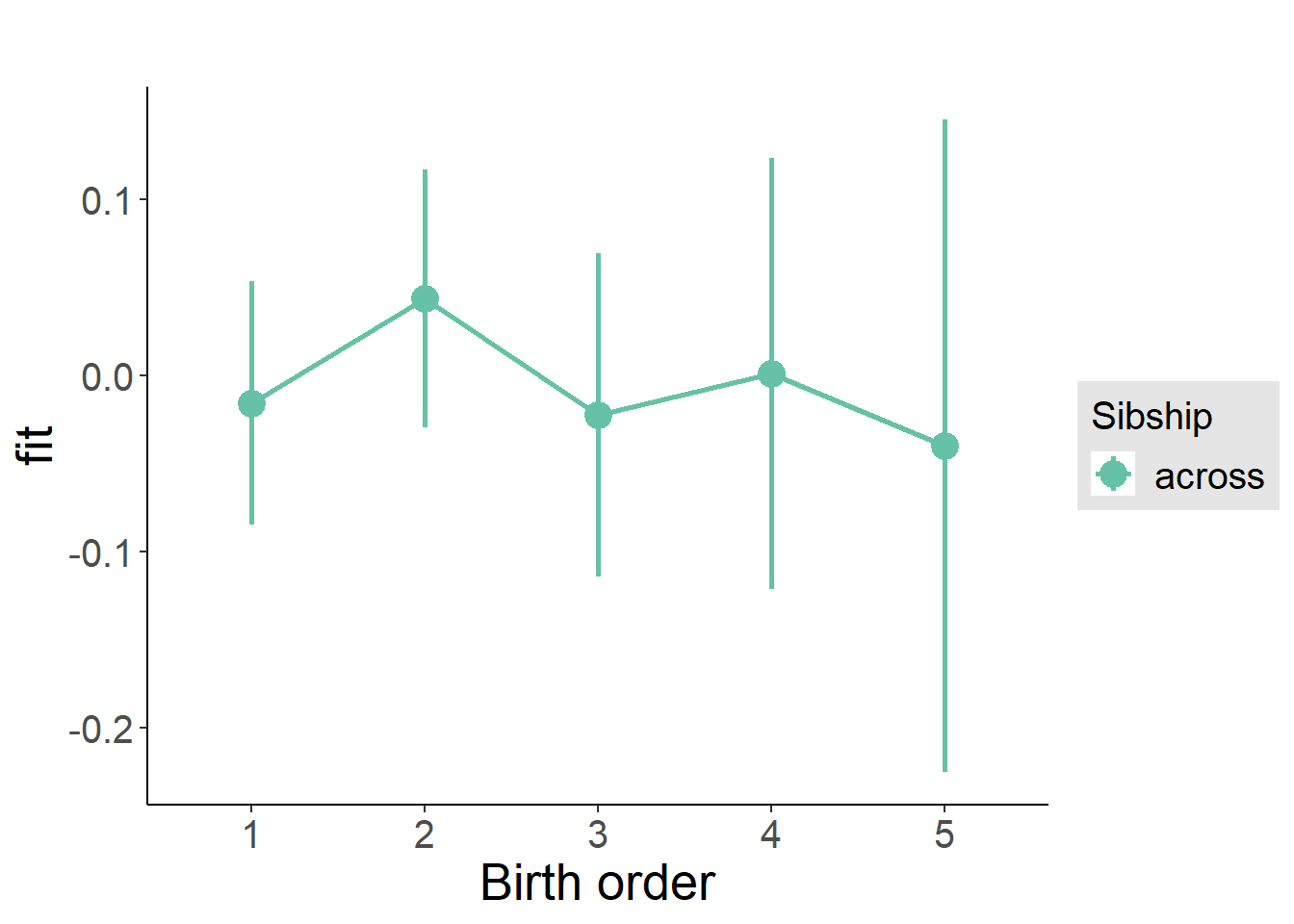
Add Interaction
Model Summary
m4_interaction = update(m3_birthorder_nonlinear, formula = . ~ . - birth_order_nonlinear - sibling_count + count_birth_order)
tidy(m4_interaction, conf.int = T, conf.level = 0.995)| effect | group | term | estimate | std.error | statistic | df | p.value | conf.low | conf.high |
|---|---|---|---|---|---|---|---|---|---|
| fixed | NA | (Intercept) | 0.4498 | 0.2014 | 2.233 | 6660 | 0.02559 | -0.1157 | 1.015 |
| fixed | NA | poly(age, 3, raw = TRUE)1 | -0.02739 | 0.01928 | -1.421 | 6448 | 0.1554 | -0.08151 | 0.02672 |
| fixed | NA | poly(age, 3, raw = TRUE)2 | 0.0007745 | 0.0005623 | 1.377 | 6209 | 0.1684 | -0.0008038 | 0.002353 |
| fixed | NA | poly(age, 3, raw = TRUE)3 | -0.00000794 | 0.000005096 | -1.558 | 6030 | 0.1192 | -0.00002224 | 0.000006364 |
| fixed | NA | male | -0.2422 | 0.02352 | -10.29 | 7092 | 1.113e-24 | -0.3082 | -0.1761 |
| fixed | NA | count_birth_order2/2 | 0.03729 | 0.04798 | 0.7771 | 5968 | 0.4371 | -0.09741 | 0.172 |
| fixed | NA | count_birth_order1/3 | 0.004145 | 0.04484 | 0.09244 | 7122 | 0.9263 | -0.1217 | 0.13 |
| fixed | NA | count_birth_order2/3 | 0.05518 | 0.05016 | 1.1 | 7127 | 0.2713 | -0.08563 | 0.196 |
| fixed | NA | count_birth_order3/3 | 0.003678 | 0.05627 | 0.06535 | 7129 | 0.9479 | -0.1543 | 0.1616 |
| fixed | NA | count_birth_order1/4 | -0.03432 | 0.05125 | -0.6697 | 7128 | 0.5031 | -0.1782 | 0.1095 |
| fixed | NA | count_birth_order2/4 | 0.0945 | 0.05391 | 1.753 | 7128 | 0.07963 | -0.05682 | 0.2458 |
| fixed | NA | count_birth_order3/4 | -0.06735 | 0.05861 | -1.149 | 7129 | 0.2506 | -0.2319 | 0.09719 |
| fixed | NA | count_birth_order4/4 | -0.05733 | 0.06212 | -0.9228 | 7128 | 0.3561 | -0.2317 | 0.117 |
| fixed | NA | count_birth_order1/5 | -0.0448 | 0.05819 | -0.7699 | 7129 | 0.4414 | -0.2081 | 0.1185 |
| fixed | NA | count_birth_order2/5 | -0.02115 | 0.06125 | -0.3453 | 7128 | 0.7299 | -0.1931 | 0.1508 |
| fixed | NA | count_birth_order3/5 | -0.006252 | 0.06288 | -0.09941 | 7127 | 0.9208 | -0.1828 | 0.1703 |
| fixed | NA | count_birth_order4/5 | 0.04315 | 0.06666 | 0.6473 | 7126 | 0.5175 | -0.144 | 0.2303 |
| fixed | NA | count_birth_order5/5 | -0.05223 | 0.06815 | -0.7663 | 7125 | 0.4435 | -0.2435 | 0.1391 |
| ran_pars | mother_pidlink | sd__(Intercept) | 0.2158 | NA | NA | NA | NA | NA | NA |
| ran_pars | Residual | sd__Observation | 0.9696 | NA | NA | NA | NA | NA | NA |
Coefficient Plot
plot_birthorder(m4_interaction)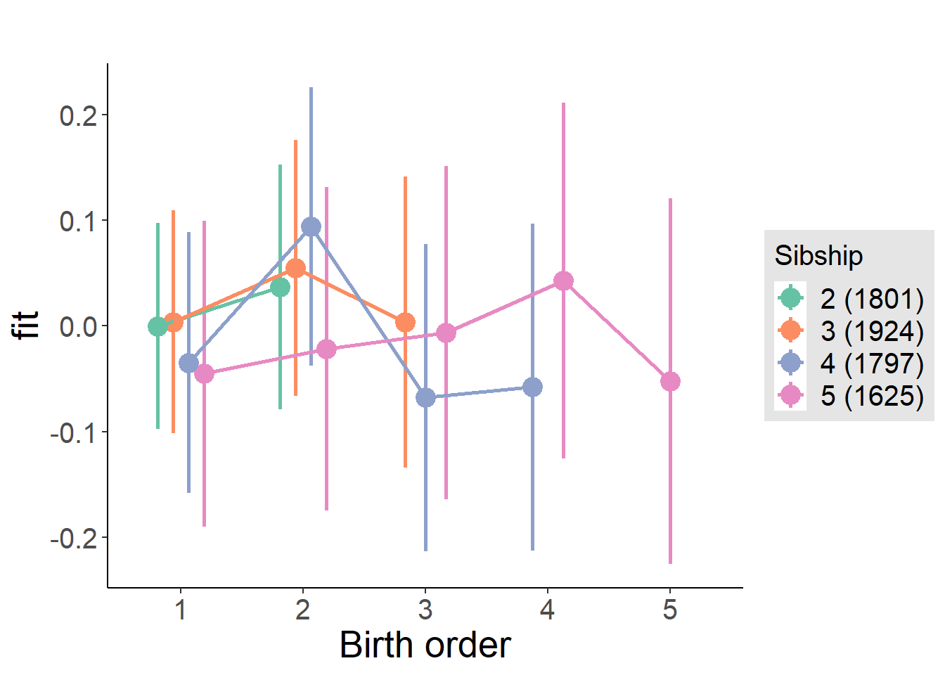
Model Comparison
###### Model 1 - Model 2
anova(m1_covariates_only, m2_birthorder_linear, m3_birthorder_nonlinear, m4_interaction)## refitting model(s) with ML (instead of REML)| Df | AIC | BIC | logLik | deviance | Chisq | Chi Df | Pr(>Chisq) |
|---|---|---|---|---|---|---|---|
| 10 | 20193 | 20262 | -10087 | 20173 | NA | NA | NA |
| 11 | 20195 | 20271 | -10087 | 20173 | 0.001739 | 1 | 0.9667 |
| 14 | 20195 | 20292 | -10084 | 20167 | 5.786 | 3 | 0.1225 |
| 20 | 20202 | 20339 | -10081 | 20162 | 5.763 | 6 | 0.4502 |
Maternal birth order
outcome_uterus_m1 <- update(m2_birthorder_linear, data = birthorder %>%
mutate(sibling_count = sibling_count_uterus_alive_factor,
birth_order_nonlinear = birthorder_uterus_alive_factor,
birth_order = birthorder_uterus_alive,
count_birth_order = count_birthorder_uterus_alive) %>%
filter(sibling_count != "1"))
compare_models_markdown(outcome_uterus_m1)Basic Model
Model Summary
m1_covariates_only <- update(m2_birthorder_linear, formula = . ~ . - birth_order)
tidy(m1_covariates_only, conf.int = T, conf.level = 0.995)| effect | group | term | estimate | std.error | statistic | df | p.value | conf.low | conf.high |
|---|---|---|---|---|---|---|---|---|---|
| fixed | NA | (Intercept) | 1.292 | 0.5584 | 2.313 | 4493 | 0.02078 | -0.276 | 2.859 |
| fixed | NA | poly(age, 3, raw = TRUE)1 | -0.115 | 0.06514 | -1.766 | 4486 | 0.07745 | -0.2979 | 0.0678 |
| fixed | NA | poly(age, 3, raw = TRUE)2 | 0.003916 | 0.002399 | 1.632 | 4477 | 0.1027 | -0.002818 | 0.01065 |
| fixed | NA | poly(age, 3, raw = TRUE)3 | -0.00004165 | 0.0000281 | -1.482 | 4468 | 0.1383 | -0.0001205 | 0.00003722 |
| fixed | NA | male | -0.2914 | 0.03016 | -9.661 | 4492 | 7.18e-22 | -0.3761 | -0.2067 |
| fixed | NA | sibling_count3 | -0.0332 | 0.0402 | -0.826 | 3343 | 0.4089 | -0.146 | 0.07963 |
| fixed | NA | sibling_count4 | -0.08768 | 0.04314 | -2.033 | 2819 | 0.04219 | -0.2088 | 0.0334 |
| fixed | NA | sibling_count5 | -0.08574 | 0.04897 | -1.751 | 2384 | 0.08008 | -0.2232 | 0.05171 |
| ran_pars | mother_pidlink | sd__(Intercept) | 0.1635 | NA | NA | NA | NA | NA | NA |
| ran_pars | Residual | sd__Observation | 0.998 | NA | NA | NA | NA | NA | NA |
Coefficient Plot
plot(allEffects(m1_covariates_only, confidence.level = 0.995))
Add Birth Order Linear
Model Summary
tidy(m2_birthorder_linear, conf.int = T, conf.level = 0.995)| effect | group | term | estimate | std.error | statistic | df | p.value | conf.low | conf.high |
|---|---|---|---|---|---|---|---|---|---|
| fixed | NA | (Intercept) | 1.24 | 0.5589 | 2.219 | 4492 | 0.02652 | -0.3285 | 2.809 |
| fixed | NA | birth_order | 0.03075 | 0.01593 | 1.93 | 4268 | 0.05362 | -0.01396 | 0.07545 |
| fixed | NA | poly(age, 3, raw = TRUE)1 | -0.1131 | 0.06512 | -1.737 | 4485 | 0.08237 | -0.296 | 0.06965 |
| fixed | NA | poly(age, 3, raw = TRUE)2 | 0.003808 | 0.002399 | 1.587 | 4476 | 0.1125 | -0.002926 | 0.01054 |
| fixed | NA | poly(age, 3, raw = TRUE)3 | -0.00003976 | 0.0000281 | -1.415 | 4468 | 0.1572 | -0.0001186 | 0.00003913 |
| fixed | NA | male | -0.2925 | 0.03016 | -9.697 | 4491 | 5.098e-22 | -0.3771 | -0.2078 |
| fixed | NA | sibling_count3 | -0.04723 | 0.04084 | -1.156 | 3406 | 0.2476 | -0.1619 | 0.0674 |
| fixed | NA | sibling_count4 | -0.1198 | 0.04621 | -2.592 | 3069 | 0.0096 | -0.2495 | 0.009959 |
| fixed | NA | sibling_count5 | -0.1394 | 0.0563 | -2.477 | 2936 | 0.01331 | -0.2975 | 0.0186 |
| ran_pars | mother_pidlink | sd__(Intercept) | 0.163 | NA | NA | NA | NA | NA | NA |
| ran_pars | Residual | sd__Observation | 0.9978 | NA | NA | NA | NA | NA | NA |
Coefficient Plot
plot_birthorder2(m2_birthorder_linear, separate = FALSE)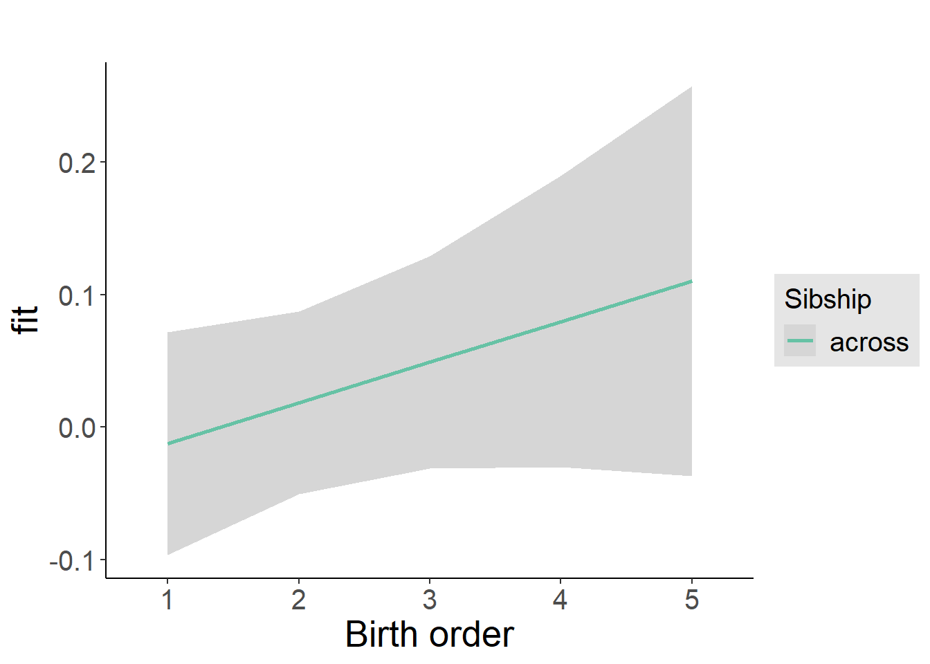
Add Birth Order Factor
Model Summary
m3_birthorder_nonlinear = update(m1_covariates_only, formula = . ~ . + birth_order_nonlinear)
tidy(m3_birthorder_nonlinear, conf.int = T, conf.level = 0.995)| effect | group | term | estimate | std.error | statistic | df | p.value | conf.low | conf.high |
|---|---|---|---|---|---|---|---|---|---|
| fixed | NA | (Intercept) | 1.282 | 0.5593 | 2.292 | 4486 | 0.02195 | -0.288 | 2.852 |
| fixed | NA | poly(age, 3, raw = TRUE)1 | -0.1146 | 0.06518 | -1.759 | 4478 | 0.07871 | -0.2976 | 0.06833 |
| fixed | NA | poly(age, 3, raw = TRUE)2 | 0.003862 | 0.002401 | 1.608 | 4469 | 0.1078 | -0.002878 | 0.0106 |
| fixed | NA | poly(age, 3, raw = TRUE)3 | -0.00004034 | 0.00002813 | -1.434 | 4461 | 0.1516 | -0.0001193 | 0.00003861 |
| fixed | NA | male | -0.2923 | 0.03017 | -9.689 | 4488 | 5.485e-22 | -0.377 | -0.2076 |
| fixed | NA | sibling_count3 | -0.03841 | 0.04154 | -0.9247 | 3535 | 0.3552 | -0.155 | 0.0782 |
| fixed | NA | sibling_count4 | -0.11 | 0.04697 | -2.341 | 3178 | 0.01927 | -0.2418 | 0.02187 |
| fixed | NA | sibling_count5 | -0.1473 | 0.05733 | -2.569 | 3021 | 0.01026 | -0.3082 | 0.01367 |
| fixed | NA | birth_order_nonlinear2 | 0.03432 | 0.03642 | 0.9424 | 3737 | 0.3461 | -0.0679 | 0.1365 |
| fixed | NA | birth_order_nonlinear3 | 0.02303 | 0.04628 | 0.4976 | 3985 | 0.6188 | -0.1069 | 0.1529 |
| fixed | NA | birth_order_nonlinear4 | 0.08706 | 0.06198 | 1.405 | 4177 | 0.1602 | -0.08693 | 0.261 |
| fixed | NA | birth_order_nonlinear5 | 0.2078 | 0.09666 | 2.15 | 4091 | 0.03165 | -0.06356 | 0.4791 |
| ran_pars | mother_pidlink | sd__(Intercept) | 0.1628 | NA | NA | NA | NA | NA | NA |
| ran_pars | Residual | sd__Observation | 0.998 | NA | NA | NA | NA | NA | NA |
Coefficient Plot
plot_birthorder(m3_birthorder_nonlinear, separate = FALSE)
Add Interaction
Model Summary
m4_interaction = update(m3_birthorder_nonlinear, formula = . ~ . - birth_order_nonlinear - sibling_count + count_birth_order)
tidy(m4_interaction, conf.int = T, conf.level = 0.995)| effect | group | term | estimate | std.error | statistic | df | p.value | conf.low | conf.high |
|---|---|---|---|---|---|---|---|---|---|
| fixed | NA | (Intercept) | 1.277 | 0.5596 | 2.283 | 4481 | 0.02248 | -0.2933 | 2.848 |
| fixed | NA | poly(age, 3, raw = TRUE)1 | -0.1141 | 0.06522 | -1.75 | 4474 | 0.08016 | -0.2972 | 0.06893 |
| fixed | NA | poly(age, 3, raw = TRUE)2 | 0.003865 | 0.002403 | 1.609 | 4465 | 0.1078 | -0.002879 | 0.01061 |
| fixed | NA | poly(age, 3, raw = TRUE)3 | -0.00004064 | 0.00002815 | -1.444 | 4457 | 0.1489 | -0.0001197 | 0.00003838 |
| fixed | NA | male | -0.2915 | 0.03019 | -9.654 | 4482 | 7.724e-22 | -0.3762 | -0.2067 |
| fixed | NA | count_birth_order2/2 | 0.02172 | 0.06239 | 0.3482 | 3846 | 0.7277 | -0.1534 | 0.1969 |
| fixed | NA | count_birth_order1/3 | -0.08163 | 0.05423 | -1.505 | 4489 | 0.1323 | -0.2339 | 0.0706 |
| fixed | NA | count_birth_order2/3 | 0.03728 | 0.05929 | 0.6288 | 4490 | 0.5295 | -0.1291 | 0.2037 |
| fixed | NA | count_birth_order3/3 | -0.008793 | 0.06633 | -0.1326 | 4488 | 0.8945 | -0.195 | 0.1774 |
| fixed | NA | count_birth_order1/4 | -0.0623 | 0.06653 | -0.9363 | 4487 | 0.3492 | -0.2491 | 0.1245 |
| fixed | NA | count_birth_order2/4 | -0.1188 | 0.06881 | -1.727 | 4490 | 0.08423 | -0.312 | 0.07431 |
| fixed | NA | count_birth_order3/4 | -0.1042 | 0.07274 | -1.432 | 4487 | 0.1522 | -0.3084 | 0.1 |
| fixed | NA | count_birth_order4/4 | -0.03789 | 0.07557 | -0.5014 | 4486 | 0.6161 | -0.25 | 0.1742 |
| fixed | NA | count_birth_order1/5 | -0.1243 | 0.09059 | -1.372 | 4490 | 0.1701 | -0.3786 | 0.13 |
| fixed | NA | count_birth_order2/5 | -0.1651 | 0.09681 | -1.705 | 4490 | 0.08818 | -0.4369 | 0.1066 |
| fixed | NA | count_birth_order3/5 | -0.1305 | 0.09073 | -1.438 | 4487 | 0.1504 | -0.3852 | 0.1242 |
| fixed | NA | count_birth_order4/5 | -0.05037 | 0.08735 | -0.5766 | 4486 | 0.5642 | -0.2956 | 0.1948 |
| fixed | NA | count_birth_order5/5 | 0.0559 | 0.09088 | 0.6151 | 4482 | 0.5385 | -0.1992 | 0.311 |
| ran_pars | mother_pidlink | sd__(Intercept) | 0.1654 | NA | NA | NA | NA | NA | NA |
| ran_pars | Residual | sd__Observation | 0.9978 | NA | NA | NA | NA | NA | NA |
Coefficient Plot
plot_birthorder(m4_interaction)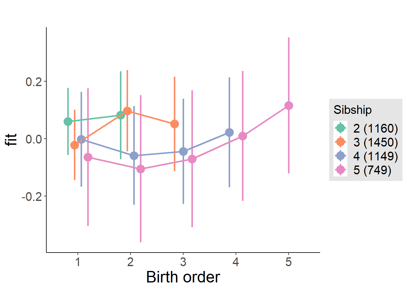
Model Comparison
###### Model 1 - Model 2
anova(m1_covariates_only, m2_birthorder_linear, m3_birthorder_nonlinear, m4_interaction)## refitting model(s) with ML (instead of REML)| Df | AIC | BIC | logLik | deviance | Chisq | Chi Df | Pr(>Chisq) |
|---|---|---|---|---|---|---|---|
| 10 | 12906 | 12970 | -6443 | 12886 | NA | NA | NA |
| 11 | 12904 | 12974 | -6441 | 12882 | 3.733 | 1 | 0.05336 |
| 14 | 12908 | 12998 | -6440 | 12880 | 1.947 | 3 | 0.5834 |
| 20 | 12916 | 13044 | -6438 | 12876 | 3.902 | 6 | 0.6899 |
Maternal pregnancy order
outcome_preg_m1 <- update(m2_birthorder_linear, data = birthorder %>%
mutate(sibling_count = sibling_count_uterus_preg_factor,
birth_order_nonlinear = birthorder_uterus_preg_factor,
birth_order = birthorder_uterus_preg,
count_birth_order = count_birthorder_uterus_preg
) %>%
filter(sibling_count != "1"))
compare_models_markdown(outcome_preg_m1)Basic Model
Model Summary
m1_covariates_only <- update(m2_birthorder_linear, formula = . ~ . - birth_order)
tidy(m1_covariates_only, conf.int = T, conf.level = 0.995)| effect | group | term | estimate | std.error | statistic | df | p.value | conf.low | conf.high |
|---|---|---|---|---|---|---|---|---|---|
| fixed | NA | (Intercept) | 1.255 | 0.5773 | 2.175 | 4173 | 0.02971 | -0.3651 | 2.876 |
| fixed | NA | poly(age, 3, raw = TRUE)1 | -0.1126 | 0.0674 | -1.67 | 4168 | 0.09495 | -0.3018 | 0.07662 |
| fixed | NA | poly(age, 3, raw = TRUE)2 | 0.003895 | 0.002483 | 1.568 | 4161 | 0.1169 | -0.003077 | 0.01087 |
| fixed | NA | poly(age, 3, raw = TRUE)3 | -0.00004159 | 0.00002909 | -1.43 | 4154 | 0.1529 | -0.0001232 | 0.00004006 |
| fixed | NA | male | -0.2858 | 0.03143 | -9.094 | 4165 | 1.445e-19 | -0.374 | -0.1976 |
| fixed | NA | sibling_count3 | -0.03749 | 0.04377 | -0.8564 | 3182 | 0.3918 | -0.1604 | 0.08538 |
| fixed | NA | sibling_count4 | -0.08365 | 0.0461 | -1.815 | 2829 | 0.0697 | -0.2131 | 0.04575 |
| fixed | NA | sibling_count5 | -0.1098 | 0.04914 | -2.235 | 2436 | 0.02551 | -0.2478 | 0.02811 |
| ran_pars | mother_pidlink | sd__(Intercept) | 0.1888 | NA | NA | NA | NA | NA | NA |
| ran_pars | Residual | sd__Observation | 0.9972 | NA | NA | NA | NA | NA | NA |
Coefficient Plot
plot(allEffects(m1_covariates_only, confidence.level = 0.995))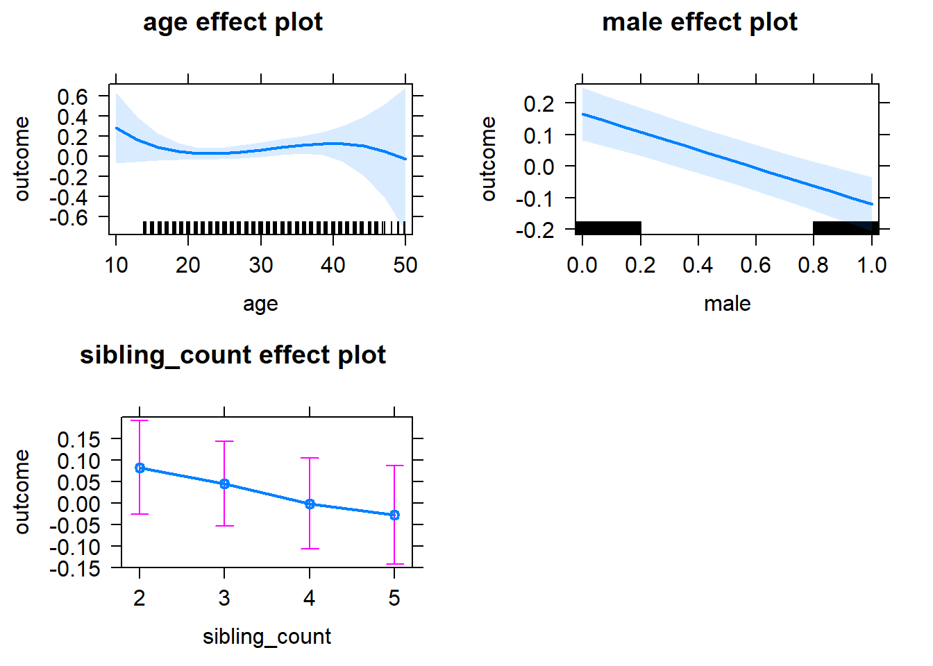
Add Birth Order Linear
Model Summary
tidy(m2_birthorder_linear, conf.int = T, conf.level = 0.995)| effect | group | term | estimate | std.error | statistic | df | p.value | conf.low | conf.high |
|---|---|---|---|---|---|---|---|---|---|
| fixed | NA | (Intercept) | 1.222 | 0.5779 | 2.114 | 4173 | 0.03454 | -0.4002 | 2.844 |
| fixed | NA | birth_order | 0.02041 | 0.01599 | 1.277 | 4018 | 0.2018 | -0.02447 | 0.06529 |
| fixed | NA | poly(age, 3, raw = TRUE)1 | -0.1114 | 0.0674 | -1.653 | 4168 | 0.09832 | -0.3006 | 0.07776 |
| fixed | NA | poly(age, 3, raw = TRUE)2 | 0.003829 | 0.002484 | 1.541 | 4161 | 0.1233 | -0.003144 | 0.0108 |
| fixed | NA | poly(age, 3, raw = TRUE)3 | -0.0000404 | 0.0000291 | -1.388 | 4154 | 0.1651 | -0.0001221 | 0.00004129 |
| fixed | NA | male | -0.2862 | 0.03143 | -9.108 | 4163 | 1.27e-19 | -0.3745 | -0.198 |
| fixed | NA | sibling_count3 | -0.04677 | 0.04438 | -1.054 | 3225 | 0.292 | -0.1713 | 0.07779 |
| fixed | NA | sibling_count4 | -0.1043 | 0.04885 | -2.135 | 3009 | 0.03288 | -0.2414 | 0.03285 |
| fixed | NA | sibling_count5 | -0.1428 | 0.05552 | -2.572 | 2863 | 0.01016 | -0.2987 | 0.01305 |
| ran_pars | mother_pidlink | sd__(Intercept) | 0.1906 | NA | NA | NA | NA | NA | NA |
| ran_pars | Residual | sd__Observation | 0.9968 | NA | NA | NA | NA | NA | NA |
Coefficient Plot
plot_birthorder2(m2_birthorder_linear, separate = FALSE)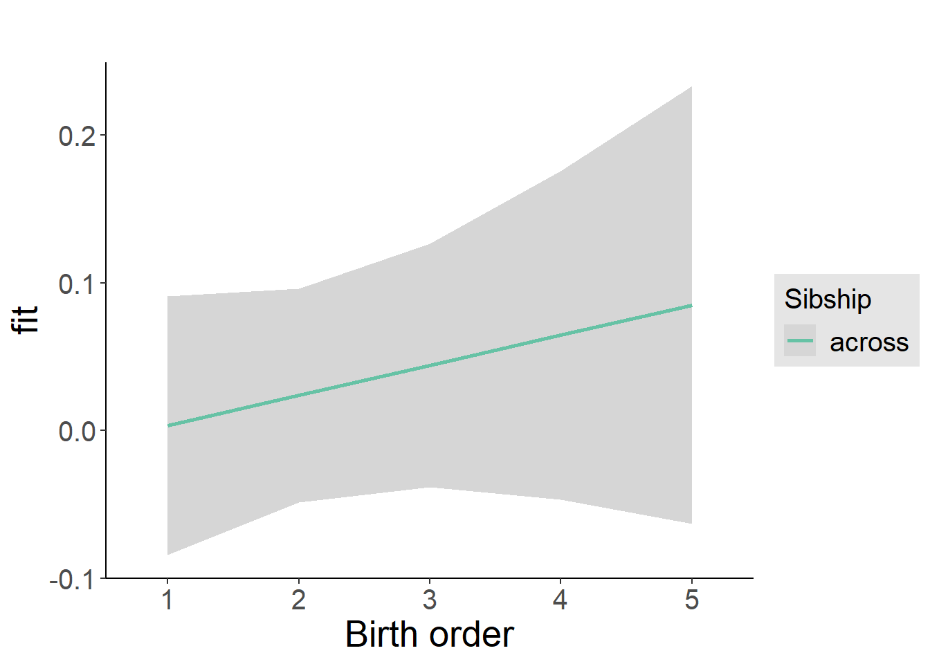
Add Birth Order Factor
Model Summary
m3_birthorder_nonlinear = update(m1_covariates_only, formula = . ~ . + birth_order_nonlinear)
tidy(m3_birthorder_nonlinear, conf.int = T, conf.level = 0.995)| effect | group | term | estimate | std.error | statistic | df | p.value | conf.low | conf.high |
|---|---|---|---|---|---|---|---|---|---|
| fixed | NA | (Intercept) | 1.241 | 0.5779 | 2.147 | 4167 | 0.03184 | -0.3814 | 2.863 |
| fixed | NA | poly(age, 3, raw = TRUE)1 | -0.1116 | 0.06742 | -1.656 | 4162 | 0.09786 | -0.3009 | 0.07763 |
| fixed | NA | poly(age, 3, raw = TRUE)2 | 0.003839 | 0.002485 | 1.545 | 4154 | 0.1224 | -0.003136 | 0.01081 |
| fixed | NA | poly(age, 3, raw = TRUE)3 | -0.00004056 | 0.00002911 | -1.393 | 4148 | 0.1636 | -0.0001223 | 0.00004115 |
| fixed | NA | male | -0.2856 | 0.03143 | -9.089 | 4160 | 1.51e-19 | -0.3738 | -0.1974 |
| fixed | NA | sibling_count3 | -0.0449 | 0.04507 | -0.9963 | 3332 | 0.3192 | -0.1714 | 0.08161 |
| fixed | NA | sibling_count4 | -0.08676 | 0.04958 | -1.75 | 3105 | 0.08021 | -0.2259 | 0.0524 |
| fixed | NA | sibling_count5 | -0.1508 | 0.05611 | -2.688 | 2908 | 0.007232 | -0.3083 | 0.006687 |
| fixed | NA | birth_order_nonlinear2 | 0.0264 | 0.03794 | 0.6958 | 3506 | 0.4866 | -0.0801 | 0.1329 |
| fixed | NA | birth_order_nonlinear3 | 0.03279 | 0.04785 | 0.6853 | 3753 | 0.4932 | -0.1015 | 0.1671 |
| fixed | NA | birth_order_nonlinear4 | -0.01721 | 0.0632 | -0.2722 | 3906 | 0.7854 | -0.1946 | 0.1602 |
| fixed | NA | birth_order_nonlinear5 | 0.2182 | 0.09272 | 2.353 | 3840 | 0.01867 | -0.04209 | 0.4784 |
| ran_pars | mother_pidlink | sd__(Intercept) | 0.1888 | NA | NA | NA | NA | NA | NA |
| ran_pars | Residual | sd__Observation | 0.9969 | NA | NA | NA | NA | NA | NA |
Coefficient Plot
plot_birthorder(m3_birthorder_nonlinear, separate = FALSE)
Add Interaction
Model Summary
m4_interaction = update(m3_birthorder_nonlinear, formula = . ~ . - birth_order_nonlinear - sibling_count + count_birth_order)
tidy(m4_interaction, conf.int = T, conf.level = 0.995)| effect | group | term | estimate | std.error | statistic | df | p.value | conf.low | conf.high |
|---|---|---|---|---|---|---|---|---|---|
| fixed | NA | (Intercept) | 1.238 | 0.5785 | 2.14 | 4161 | 0.03241 | -0.3858 | 2.862 |
| fixed | NA | poly(age, 3, raw = TRUE)1 | -0.1109 | 0.06747 | -1.643 | 4156 | 0.1004 | -0.3003 | 0.07852 |
| fixed | NA | poly(age, 3, raw = TRUE)2 | 0.003821 | 0.002487 | 1.536 | 4149 | 0.1245 | -0.00316 | 0.0108 |
| fixed | NA | poly(age, 3, raw = TRUE)3 | -0.00004046 | 0.00002914 | -1.389 | 4142 | 0.165 | -0.0001223 | 0.00004133 |
| fixed | NA | male | -0.2856 | 0.03145 | -9.08 | 4154 | 1.639e-19 | -0.3739 | -0.1973 |
| fixed | NA | count_birth_order2/2 | 0.01054 | 0.06836 | 0.1541 | 3607 | 0.8775 | -0.1813 | 0.2024 |
| fixed | NA | count_birth_order1/3 | -0.08448 | 0.05893 | -1.433 | 4166 | 0.1518 | -0.2499 | 0.08095 |
| fixed | NA | count_birth_order2/3 | 0.01745 | 0.06393 | 0.273 | 4167 | 0.7849 | -0.162 | 0.1969 |
| fixed | NA | count_birth_order3/3 | -0.01086 | 0.07201 | -0.1508 | 4165 | 0.8801 | -0.213 | 0.1913 |
| fixed | NA | count_birth_order1/4 | -0.05595 | 0.06996 | -0.7997 | 4165 | 0.4239 | -0.2523 | 0.1404 |
| fixed | NA | count_birth_order2/4 | -0.07123 | 0.07123 | -1 | 4167 | 0.3173 | -0.2712 | 0.1287 |
| fixed | NA | count_birth_order3/4 | -0.07095 | 0.07817 | -0.9077 | 4164 | 0.3641 | -0.2904 | 0.1485 |
| fixed | NA | count_birth_order4/4 | -0.145 | 0.08051 | -1.801 | 4163 | 0.07183 | -0.371 | 0.08103 |
| fixed | NA | count_birth_order1/5 | -0.1363 | 0.08325 | -1.637 | 4166 | 0.1016 | -0.37 | 0.09737 |
| fixed | NA | count_birth_order2/5 | -0.2032 | 0.08926 | -2.277 | 4167 | 0.02285 | -0.4538 | 0.04733 |
| fixed | NA | count_birth_order3/5 | -0.1196 | 0.08672 | -1.38 | 4165 | 0.1678 | -0.3631 | 0.1238 |
| fixed | NA | count_birth_order4/5 | -0.1273 | 0.08986 | -1.417 | 4160 | 0.1566 | -0.3796 | 0.1249 |
| fixed | NA | count_birth_order5/5 | 0.06195 | 0.09005 | 0.688 | 4157 | 0.4915 | -0.1908 | 0.3147 |
| ran_pars | mother_pidlink | sd__(Intercept) | 0.1876 | NA | NA | NA | NA | NA | NA |
| ran_pars | Residual | sd__Observation | 0.9974 | NA | NA | NA | NA | NA | NA |
Coefficient Plot
plot_birthorder(m4_interaction)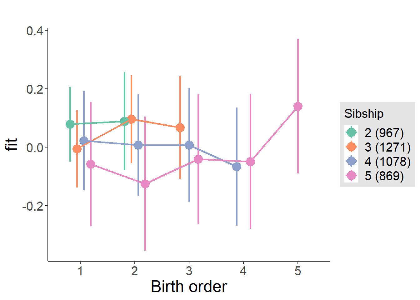
Model Comparison
###### Model 1 - Model 2
anova(m1_covariates_only, m2_birthorder_linear, m3_birthorder_nonlinear, m4_interaction)## refitting model(s) with ML (instead of REML)| Df | AIC | BIC | logLik | deviance | Chisq | Chi Df | Pr(>Chisq) |
|---|---|---|---|---|---|---|---|
| 10 | 12011 | 12074 | -5995 | 11991 | NA | NA | NA |
| 11 | 12011 | 12081 | -5995 | 11989 | 1.63 | 1 | 0.2017 |
| 14 | 12012 | 12101 | -5992 | 11984 | 4.952 | 3 | 0.1753 |
| 20 | 12021 | 12147 | -5990 | 11981 | 3.454 | 6 | 0.75 |
Parental full sibling order
outcome_parental_m1 <- update(m2_birthorder_linear, data = birthorder %>%
mutate(sibling_count = sibling_count_genes_factor,
birth_order_nonlinear = birthorder_genes_factor,
birth_order = birthorder_genes,
count_birth_order = count_birthorder_genes
) %>%
filter(sibling_count != "1"))
compare_models_markdown(outcome_parental_m1)Basic Model
Model Summary
m1_covariates_only <- update(m2_birthorder_linear, formula = . ~ . - birth_order)
tidy(m1_covariates_only, conf.int = T, conf.level = 0.995)| effect | group | term | estimate | std.error | statistic | df | p.value | conf.low | conf.high |
|---|---|---|---|---|---|---|---|---|---|
| fixed | NA | (Intercept) | 1.114 | 0.5627 | 1.98 | 4478 | 0.04782 | -0.4656 | 2.693 |
| fixed | NA | poly(age, 3, raw = TRUE)1 | -0.09265 | 0.06572 | -1.41 | 4470 | 0.1587 | -0.2771 | 0.09182 |
| fixed | NA | poly(age, 3, raw = TRUE)2 | 0.003106 | 0.002424 | 1.281 | 4460 | 0.2002 | -0.003698 | 0.00991 |
| fixed | NA | poly(age, 3, raw = TRUE)3 | -0.00003262 | 0.00002844 | -1.147 | 4451 | 0.2515 | -0.0001125 | 0.00004721 |
| fixed | NA | male | -0.2954 | 0.03018 | -9.79 | 4478 | 2.077e-22 | -0.3801 | -0.2107 |
| fixed | NA | sibling_count3 | -0.04275 | 0.03959 | -1.08 | 3310 | 0.2804 | -0.1539 | 0.06839 |
| fixed | NA | sibling_count4 | -0.07902 | 0.04273 | -1.849 | 2802 | 0.06454 | -0.199 | 0.04093 |
| fixed | NA | sibling_count5 | -0.1128 | 0.04997 | -2.257 | 2255 | 0.0241 | -0.253 | 0.02748 |
| ran_pars | mother_pidlink | sd__(Intercept) | 0.1587 | NA | NA | NA | NA | NA | NA |
| ran_pars | Residual | sd__Observation | 0.9969 | NA | NA | NA | NA | NA | NA |
Coefficient Plot
plot(allEffects(m1_covariates_only, confidence.level = 0.995))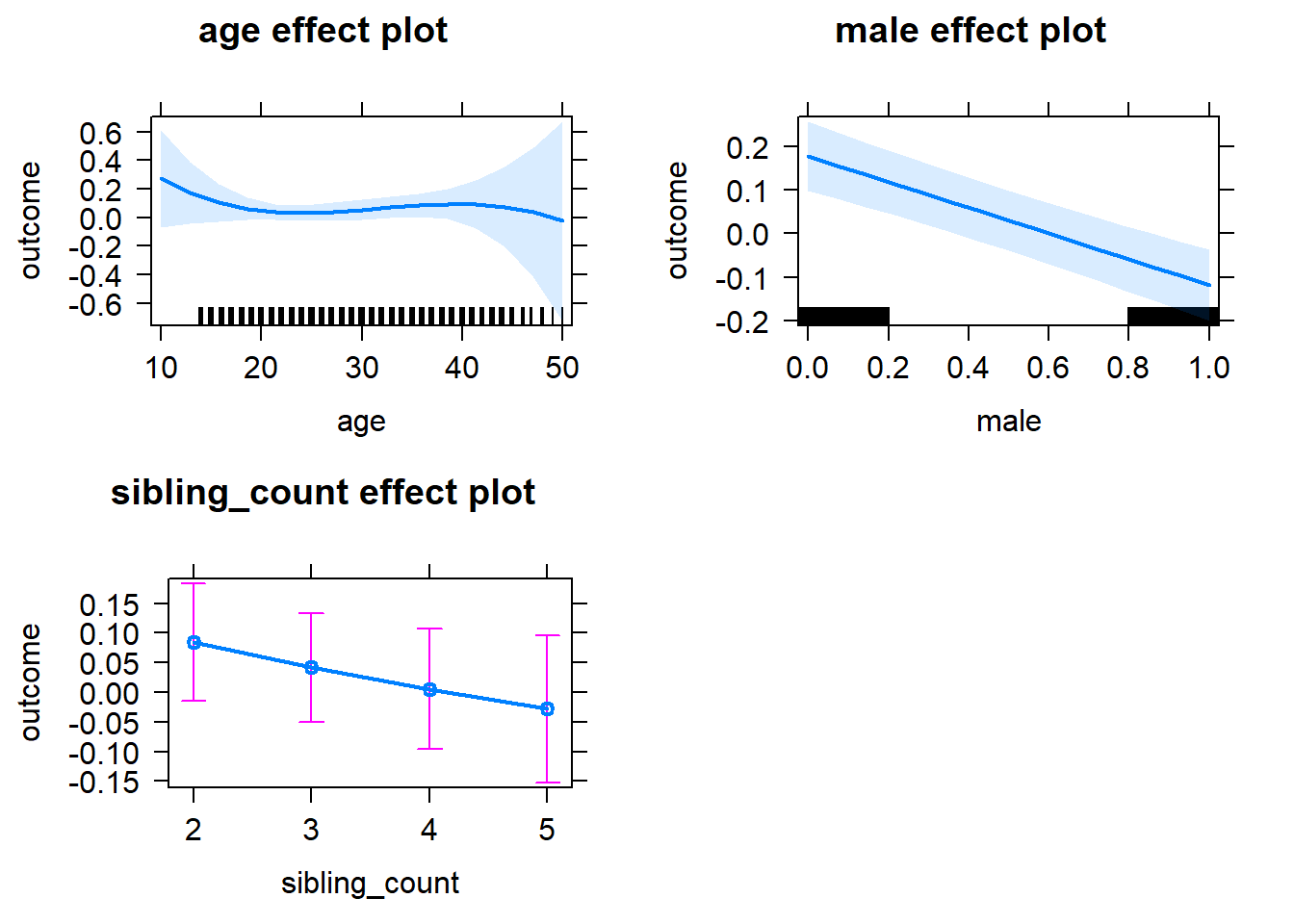
Add Birth Order Linear
Model Summary
tidy(m2_birthorder_linear, conf.int = T, conf.level = 0.995)| effect | group | term | estimate | std.error | statistic | df | p.value | conf.low | conf.high |
|---|---|---|---|---|---|---|---|---|---|
| fixed | NA | (Intercept) | 1.055 | 0.563 | 1.874 | 4476 | 0.06097 | -0.5252 | 2.636 |
| fixed | NA | birth_order | 0.03612 | 0.01612 | 2.241 | 4241 | 0.02507 | -0.009119 | 0.08136 |
| fixed | NA | poly(age, 3, raw = TRUE)1 | -0.09067 | 0.06569 | -1.38 | 4469 | 0.1676 | -0.2751 | 0.09373 |
| fixed | NA | poly(age, 3, raw = TRUE)2 | 0.002988 | 0.002423 | 1.233 | 4459 | 0.2176 | -0.003815 | 0.009791 |
| fixed | NA | poly(age, 3, raw = TRUE)3 | -0.00003051 | 0.00002844 | -1.073 | 4450 | 0.2834 | -0.0001104 | 0.00004933 |
| fixed | NA | male | -0.2964 | 0.03017 | -9.827 | 4477 | 1.46e-22 | -0.3811 | -0.2117 |
| fixed | NA | sibling_count3 | -0.05915 | 0.04025 | -1.47 | 3369 | 0.1418 | -0.1721 | 0.05383 |
| fixed | NA | sibling_count4 | -0.1166 | 0.04588 | -2.541 | 3065 | 0.01111 | -0.2454 | 0.01222 |
| fixed | NA | sibling_count5 | -0.1729 | 0.0567 | -3.05 | 2755 | 0.002311 | -0.3321 | -0.01377 |
| ran_pars | mother_pidlink | sd__(Intercept) | 0.1587 | NA | NA | NA | NA | NA | NA |
| ran_pars | Residual | sd__Observation | 0.9965 | NA | NA | NA | NA | NA | NA |
Coefficient Plot
plot_birthorder2(m2_birthorder_linear, separate = FALSE)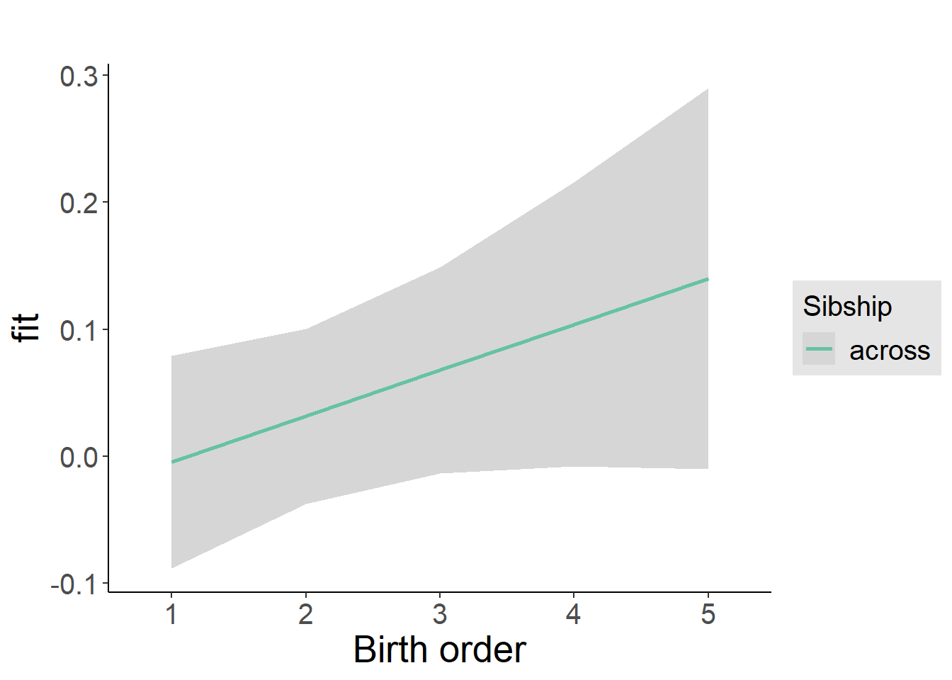
Add Birth Order Factor
Model Summary
m3_birthorder_nonlinear = update(m1_covariates_only, formula = . ~ . + birth_order_nonlinear)
tidy(m3_birthorder_nonlinear, conf.int = T, conf.level = 0.995)| effect | group | term | estimate | std.error | statistic | df | p.value | conf.low | conf.high |
|---|---|---|---|---|---|---|---|---|---|
| fixed | NA | (Intercept) | 1.098 | 0.5634 | 1.949 | 4470 | 0.0513 | -0.4831 | 2.68 |
| fixed | NA | poly(age, 3, raw = TRUE)1 | -0.0916 | 0.06575 | -1.393 | 4462 | 0.1637 | -0.2762 | 0.09298 |
| fixed | NA | poly(age, 3, raw = TRUE)2 | 0.003021 | 0.002426 | 1.245 | 4452 | 0.2131 | -0.003788 | 0.009829 |
| fixed | NA | poly(age, 3, raw = TRUE)3 | -0.00003084 | 0.00002847 | -1.083 | 4443 | 0.2787 | -0.0001108 | 0.00004907 |
| fixed | NA | male | -0.2969 | 0.03018 | -9.839 | 4474 | 1.301e-22 | -0.3816 | -0.2122 |
| fixed | NA | sibling_count3 | -0.05314 | 0.04098 | -1.297 | 3506 | 0.1948 | -0.1682 | 0.0619 |
| fixed | NA | sibling_count4 | -0.1177 | 0.04665 | -2.523 | 3176 | 0.01169 | -0.2486 | 0.01326 |
| fixed | NA | sibling_count5 | -0.1727 | 0.05794 | -2.981 | 2847 | 0.002898 | -0.3354 | -0.01008 |
| fixed | NA | birth_order_nonlinear2 | 0.03917 | 0.03616 | 1.083 | 3727 | 0.2788 | -0.06233 | 0.1407 |
| fixed | NA | birth_order_nonlinear3 | 0.04696 | 0.04609 | 1.019 | 3948 | 0.3083 | -0.08241 | 0.1763 |
| fixed | NA | birth_order_nonlinear4 | 0.1435 | 0.06325 | 2.268 | 4157 | 0.02336 | -0.03407 | 0.321 |
| fixed | NA | birth_order_nonlinear5 | 0.1306 | 0.1033 | 1.265 | 4141 | 0.2061 | -0.1593 | 0.4206 |
| ran_pars | mother_pidlink | sd__(Intercept) | 0.1578 | NA | NA | NA | NA | NA | NA |
| ran_pars | Residual | sd__Observation | 0.9968 | NA | NA | NA | NA | NA | NA |
Coefficient Plot
plot_birthorder(m3_birthorder_nonlinear, separate = FALSE)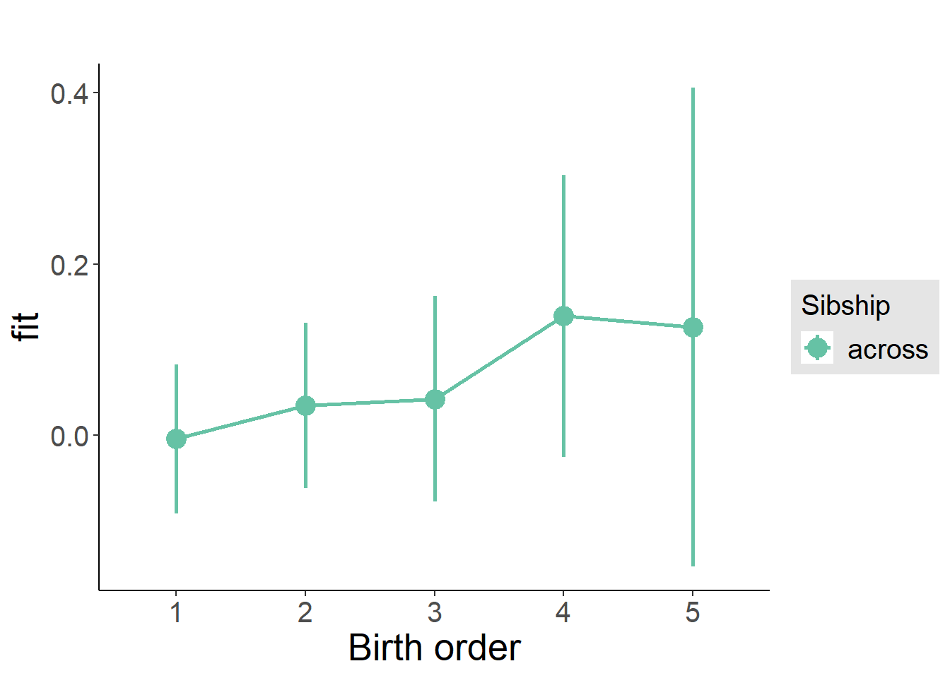
Add Interaction
Model Summary
m4_interaction = update(m3_birthorder_nonlinear, formula = . ~ . - birth_order_nonlinear - sibling_count + count_birth_order)
tidy(m4_interaction, conf.int = T, conf.level = 0.995)| effect | group | term | estimate | std.error | statistic | df | p.value | conf.low | conf.high |
|---|---|---|---|---|---|---|---|---|---|
| fixed | NA | (Intercept) | 1.098 | 0.5639 | 1.948 | 4464 | 0.05153 | -0.4846 | 2.681 |
| fixed | NA | poly(age, 3, raw = TRUE)1 | -0.09102 | 0.06581 | -1.383 | 4458 | 0.1667 | -0.2758 | 0.09371 |
| fixed | NA | poly(age, 3, raw = TRUE)2 | 0.003015 | 0.002428 | 1.242 | 4448 | 0.2144 | -0.0038 | 0.00983 |
| fixed | NA | poly(age, 3, raw = TRUE)3 | -0.00003096 | 0.0000285 | -1.087 | 4439 | 0.2772 | -0.000111 | 0.00004902 |
| fixed | NA | male | -0.2964 | 0.0302 | -9.813 | 4468 | 1.673e-22 | -0.3812 | -0.2116 |
| fixed | NA | count_birth_order2/2 | 0.01571 | 0.06073 | 0.2586 | 3815 | 0.7959 | -0.1548 | 0.1862 |
| fixed | NA | count_birth_order1/3 | -0.08884 | 0.05349 | -1.661 | 4474 | 0.0968 | -0.239 | 0.06131 |
| fixed | NA | count_birth_order2/3 | 0.009791 | 0.05918 | 0.1654 | 4475 | 0.8686 | -0.1563 | 0.1759 |
| fixed | NA | count_birth_order3/3 | -0.004587 | 0.06508 | -0.07048 | 4472 | 0.9438 | -0.1873 | 0.1781 |
| fixed | NA | count_birth_order1/4 | -0.1022 | 0.06675 | -1.531 | 4473 | 0.1259 | -0.2895 | 0.0852 |
| fixed | NA | count_birth_order2/4 | -0.1114 | 0.0686 | -1.624 | 4475 | 0.1045 | -0.3039 | 0.08117 |
| fixed | NA | count_birth_order3/4 | -0.08587 | 0.07189 | -1.195 | 4472 | 0.2323 | -0.2877 | 0.1159 |
| fixed | NA | count_birth_order4/4 | 0.02402 | 0.07595 | 0.3163 | 4470 | 0.7518 | -0.1892 | 0.2372 |
| fixed | NA | count_birth_order1/5 | -0.1552 | 0.09022 | -1.721 | 4474 | 0.08539 | -0.4085 | 0.09802 |
| fixed | NA | count_birth_order2/5 | -0.1484 | 0.09962 | -1.49 | 4475 | 0.1364 | -0.428 | 0.1312 |
| fixed | NA | count_birth_order3/5 | -0.1456 | 0.09496 | -1.533 | 4472 | 0.1253 | -0.4122 | 0.121 |
| fixed | NA | count_birth_order4/5 | -0.04816 | 0.09145 | -0.5266 | 4472 | 0.5985 | -0.3048 | 0.2085 |
| fixed | NA | count_birth_order5/5 | -0.05059 | 0.09714 | -0.5208 | 4469 | 0.6025 | -0.3233 | 0.2221 |
| ran_pars | mother_pidlink | sd__(Intercept) | 0.1587 | NA | NA | NA | NA | NA | NA |
| ran_pars | Residual | sd__Observation | 0.9972 | NA | NA | NA | NA | NA | NA |
Coefficient Plot
plot_birthorder(m4_interaction)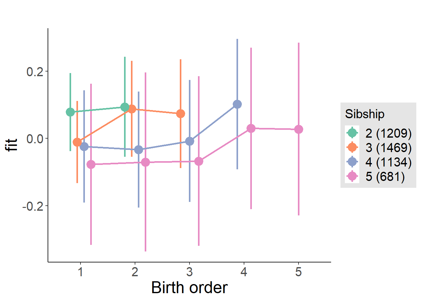
Model Comparison
###### Model 1 - Model 2
anova(m1_covariates_only, m2_birthorder_linear, m3_birthorder_nonlinear, m4_interaction)## refitting model(s) with ML (instead of REML)| Df | AIC | BIC | logLik | deviance | Chisq | Chi Df | Pr(>Chisq) |
|---|---|---|---|---|---|---|---|
| 10 | 12846 | 12910 | -6413 | 12826 | NA | NA | NA |
| 11 | 12843 | 12914 | -6411 | 12821 | 5.03 | 1 | 0.02491 |
| 14 | 12848 | 12938 | -6410 | 12820 | 0.9274 | 3 | 0.8188 |
| 20 | 12859 | 12987 | -6409 | 12819 | 1.677 | 6 | 0.9469 |
Compare birth order specifications
library(coefplot)
multiplot(outcome_naive_m1, outcome_preg_m1, outcome_uterus_m1, outcome_parental_m1, dodgeHeight = 0.6,
intercept = FALSE)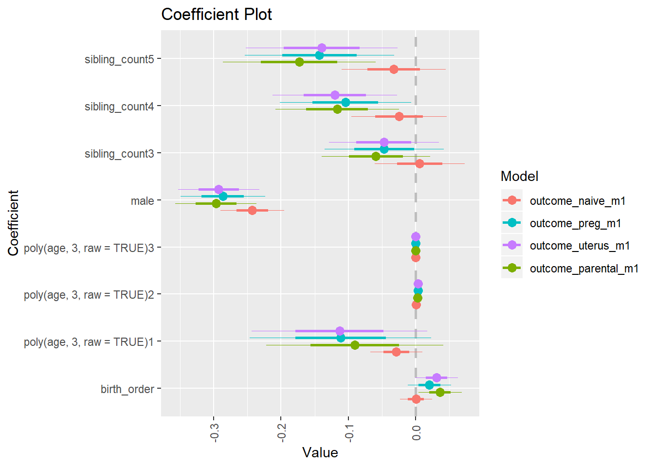
Neuroticism
birthorder <- birthorder %>% mutate(outcome = big5_neu)
model = lmer(outcome ~ birth_order + poly(age, 3, raw = TRUE) + male + sibling_count + (1 | mother_pidlink),
data = birthorder)
compare_birthorder_specs(model)Naive birth order
outcome_naive_m1 <- update(m2_birthorder_linear, data = birthorder %>%
mutate(sibling_count = sibling_count_naive_factor,
birth_order_nonlinear = birthorder_naive_factor,
birth_order = birthorder_naive,
count_birth_order = count_birthorder_naive) %>%
filter(sibling_count != "1"))
compare_models_markdown(outcome_naive_m1)Basic Model
Model Summary
m1_covariates_only <- update(m2_birthorder_linear, formula = . ~ . - birth_order)
tidy(m1_covariates_only, conf.int = T, conf.level = 0.995)| effect | group | term | estimate | std.error | statistic | df | p.value | conf.low | conf.high |
|---|---|---|---|---|---|---|---|---|---|
| fixed | NA | (Intercept) | 0.4764 | 0.1993 | 2.39 | 6737 | 0.01687 | -0.0831 | 1.036 |
| fixed | NA | poly(age, 3, raw = TRUE)1 | -0.006945 | 0.01915 | -0.3627 | 6567 | 0.7169 | -0.0607 | 0.04681 |
| fixed | NA | poly(age, 3, raw = TRUE)2 | -0.0002754 | 0.0005593 | -0.4924 | 6372 | 0.6224 | -0.001845 | 0.001295 |
| fixed | NA | poly(age, 3, raw = TRUE)3 | 0.000003654 | 0.000005075 | 0.7201 | 6220 | 0.4715 | -0.00001059 | 0.0000179 |
| fixed | NA | male | -0.2908 | 0.0232 | -12.53 | 7047 | 1.18e-35 | -0.3559 | -0.2257 |
| fixed | NA | sibling_count3 | -0.009614 | 0.03327 | -0.2889 | 5006 | 0.7726 | -0.103 | 0.08379 |
| fixed | NA | sibling_count4 | -0.002416 | 0.03429 | -0.07046 | 4453 | 0.9438 | -0.09868 | 0.09385 |
| fixed | NA | sibling_count5 | -0.04077 | 0.03566 | -1.143 | 3873 | 0.2529 | -0.1409 | 0.05932 |
| ran_pars | mother_pidlink | sd__(Intercept) | 0.3044 | NA | NA | NA | NA | NA | NA |
| ran_pars | Residual | sd__Observation | 0.9355 | NA | NA | NA | NA | NA | NA |
Coefficient Plot
plot(allEffects(m1_covariates_only, confidence.level = 0.995))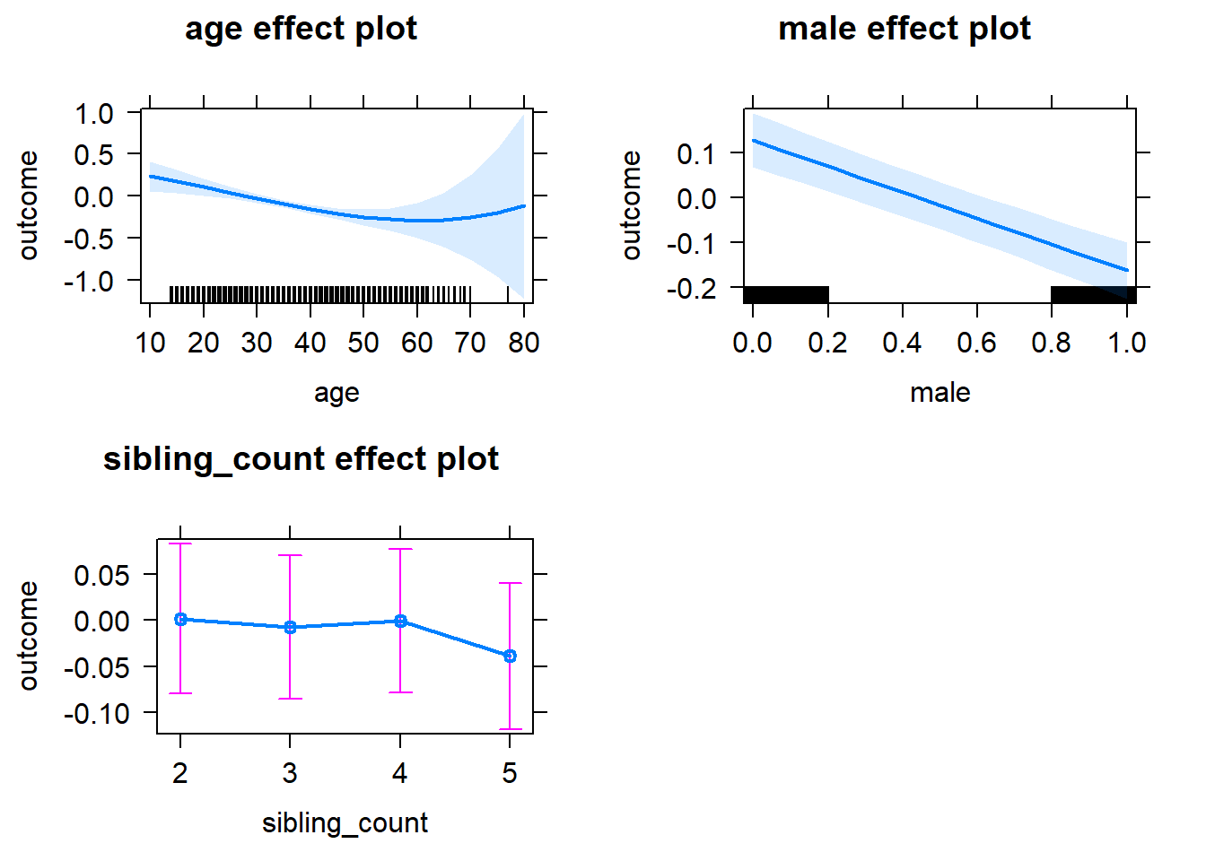
Add Birth Order Linear
Model Summary
tidy(m2_birthorder_linear, conf.int = T, conf.level = 0.995)| effect | group | term | estimate | std.error | statistic | df | p.value | conf.low | conf.high |
|---|---|---|---|---|---|---|---|---|---|
| fixed | NA | (Intercept) | 0.4816 | 0.1994 | 2.416 | 6726 | 0.01574 | -0.07803 | 1.041 |
| fixed | NA | birth_order | -0.01358 | 0.01159 | -1.172 | 6101 | 0.2411 | -0.0461 | 0.01894 |
| fixed | NA | poly(age, 3, raw = TRUE)1 | -0.005613 | 0.01918 | -0.2926 | 6593 | 0.7698 | -0.05946 | 0.04823 |
| fixed | NA | poly(age, 3, raw = TRUE)2 | -0.0003095 | 0.0005601 | -0.5526 | 6387 | 0.5806 | -0.001882 | 0.001263 |
| fixed | NA | poly(age, 3, raw = TRUE)3 | 0.000003875 | 0.000005079 | 0.763 | 6228 | 0.4455 | -0.00001038 | 0.00001813 |
| fixed | NA | male | -0.2904 | 0.02321 | -12.51 | 7046 | 1.475e-35 | -0.3556 | -0.2253 |
| fixed | NA | sibling_count3 | -0.004777 | 0.03353 | -0.1425 | 5137 | 0.8867 | -0.09889 | 0.08933 |
| fixed | NA | sibling_count4 | 0.008855 | 0.03561 | 0.2486 | 5002 | 0.8036 | -0.09111 | 0.1088 |
| fixed | NA | sibling_count5 | -0.02262 | 0.03887 | -0.5818 | 4971 | 0.5607 | -0.1317 | 0.0865 |
| ran_pars | mother_pidlink | sd__(Intercept) | 0.3041 | NA | NA | NA | NA | NA | NA |
| ran_pars | Residual | sd__Observation | 0.9355 | NA | NA | NA | NA | NA | NA |
Coefficient Plot
plot_birthorder2(m2_birthorder_linear, separate = FALSE)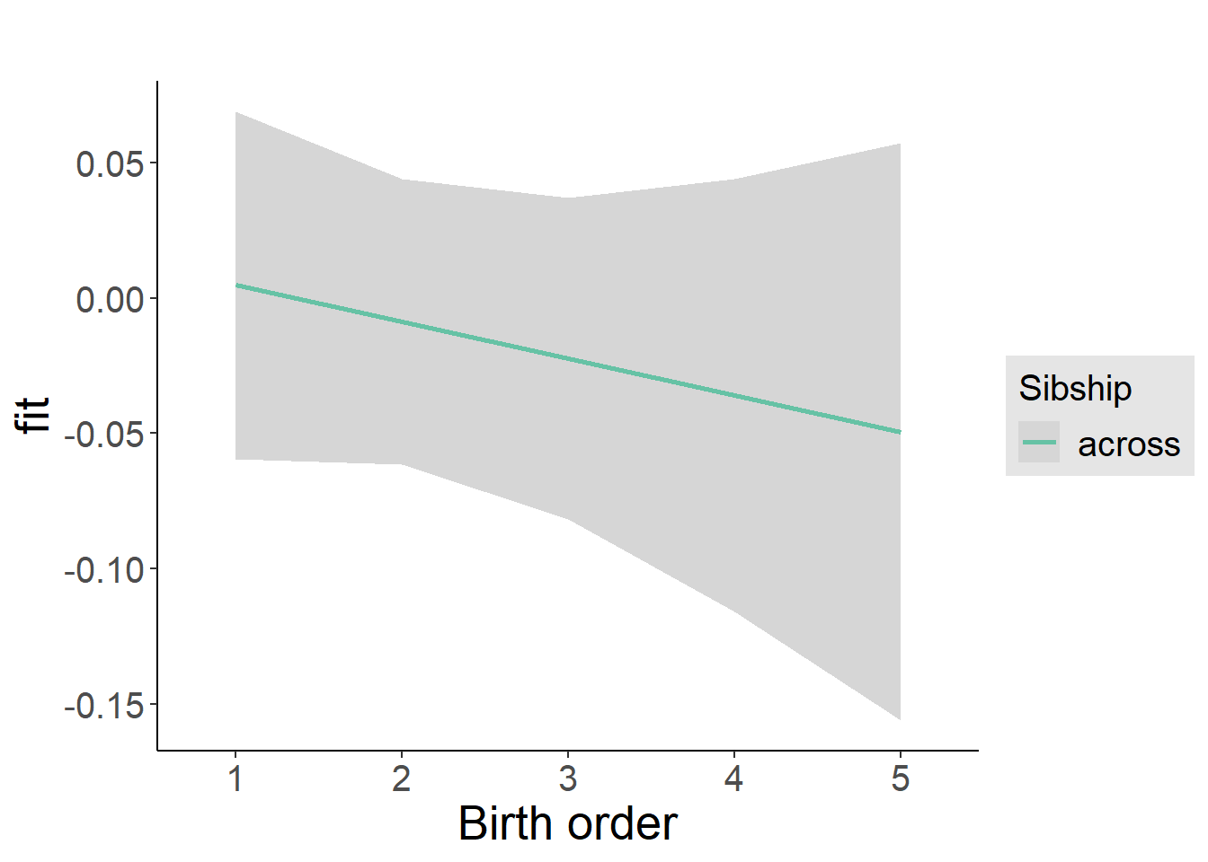
Add Birth Order Factor
Model Summary
m3_birthorder_nonlinear = update(m1_covariates_only, formula = . ~ . + birth_order_nonlinear)
tidy(m3_birthorder_nonlinear, conf.int = T, conf.level = 0.995)| effect | group | term | estimate | std.error | statistic | df | p.value | conf.low | conf.high |
|---|---|---|---|---|---|---|---|---|---|
| fixed | NA | (Intercept) | 0.4589 | 0.1999 | 2.295 | 6748 | 0.02174 | -0.1023 | 1.02 |
| fixed | NA | poly(age, 3, raw = TRUE)1 | -0.00526 | 0.01919 | -0.2741 | 6579 | 0.784 | -0.05914 | 0.04862 |
| fixed | NA | poly(age, 3, raw = TRUE)2 | -0.0003274 | 0.0005605 | -0.5841 | 6363 | 0.5592 | -0.001901 | 0.001246 |
| fixed | NA | poly(age, 3, raw = TRUE)3 | 0.0000041 | 0.000005085 | 0.8063 | 6192 | 0.4201 | -0.00001017 | 0.00001837 |
| fixed | NA | male | -0.2905 | 0.02321 | -12.52 | 7043 | 1.459e-35 | -0.3556 | -0.2253 |
| fixed | NA | sibling_count3 | -0.007908 | 0.03405 | -0.2322 | 5353 | 0.8164 | -0.1035 | 0.08769 |
| fixed | NA | sibling_count4 | 0.005984 | 0.0362 | 0.1653 | 5246 | 0.8687 | -0.09563 | 0.1076 |
| fixed | NA | sibling_count5 | -0.01713 | 0.03925 | -0.4365 | 5148 | 0.6625 | -0.1273 | 0.09303 |
| fixed | NA | birth_order_nonlinear2 | 0.00793 | 0.02753 | 0.288 | 5981 | 0.7734 | -0.06936 | 0.08522 |
| fixed | NA | birth_order_nonlinear3 | -0.00762 | 0.03534 | -0.2156 | 5930 | 0.8293 | -0.1068 | 0.09157 |
| fixed | NA | birth_order_nonlinear4 | -0.03616 | 0.04615 | -0.7835 | 5932 | 0.4334 | -0.1657 | 0.09339 |
| fixed | NA | birth_order_nonlinear5 | -0.09561 | 0.06715 | -1.424 | 5807 | 0.1546 | -0.2841 | 0.09289 |
| ran_pars | mother_pidlink | sd__(Intercept) | 0.3036 | NA | NA | NA | NA | NA | NA |
| ran_pars | Residual | sd__Observation | 0.9358 | NA | NA | NA | NA | NA | NA |
Coefficient Plot
plot_birthorder(m3_birthorder_nonlinear, separate = FALSE)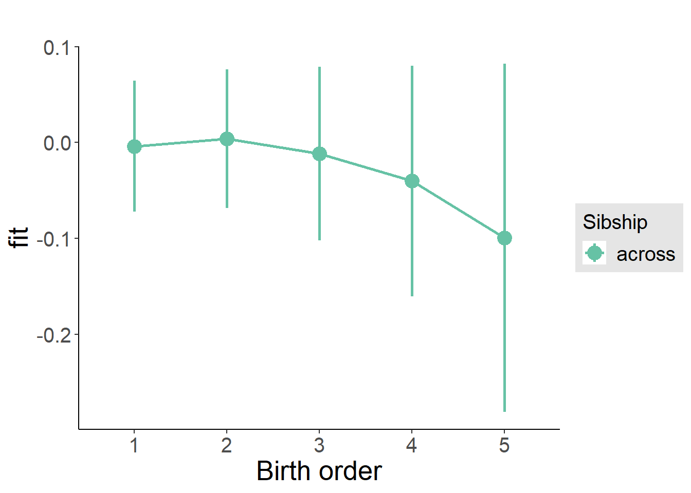
Add Interaction
Model Summary
m4_interaction = update(m3_birthorder_nonlinear, formula = . ~ . - birth_order_nonlinear - sibling_count + count_birth_order)
tidy(m4_interaction, conf.int = T, conf.level = 0.995)| effect | group | term | estimate | std.error | statistic | df | p.value | conf.low | conf.high |
|---|---|---|---|---|---|---|---|---|---|
| fixed | NA | (Intercept) | 0.4578 | 0.2004 | 2.285 | 6751 | 0.02236 | -0.1047 | 1.02 |
| fixed | NA | poly(age, 3, raw = TRUE)1 | -0.005241 | 0.0192 | -0.273 | 6575 | 0.7849 | -0.05914 | 0.04865 |
| fixed | NA | poly(age, 3, raw = TRUE)2 | -0.0003285 | 0.0005607 | -0.5859 | 6354 | 0.558 | -0.001902 | 0.001245 |
| fixed | NA | poly(age, 3, raw = TRUE)3 | 0.000004111 | 0.000005086 | 0.8082 | 6180 | 0.419 | -0.00001017 | 0.00001839 |
| fixed | NA | male | -0.2906 | 0.02322 | -12.51 | 7036 | 1.515e-35 | -0.3558 | -0.2254 |
| fixed | NA | count_birth_order2/2 | 0.01125 | 0.04701 | 0.2393 | 5937 | 0.8109 | -0.1207 | 0.1432 |
| fixed | NA | count_birth_order1/3 | -0.0001867 | 0.04439 | -0.004206 | 7110 | 0.9966 | -0.1248 | 0.1244 |
| fixed | NA | count_birth_order2/3 | -0.008199 | 0.04964 | -0.1651 | 7125 | 0.8688 | -0.1476 | 0.1312 |
| fixed | NA | count_birth_order3/3 | -0.01451 | 0.05566 | -0.2607 | 7128 | 0.7943 | -0.1707 | 0.1417 |
| fixed | NA | count_birth_order1/4 | -0.01966 | 0.05071 | -0.3876 | 7126 | 0.6983 | -0.162 | 0.1227 |
| fixed | NA | count_birth_order2/4 | 0.02814 | 0.05334 | 0.5275 | 7128 | 0.5979 | -0.1216 | 0.1779 |
| fixed | NA | count_birth_order3/4 | 0.01074 | 0.05797 | 0.1852 | 7127 | 0.8531 | -0.152 | 0.1735 |
| fixed | NA | count_birth_order4/4 | -0.01446 | 0.06142 | -0.2355 | 7122 | 0.8139 | -0.1869 | 0.158 |
| fixed | NA | count_birth_order1/5 | 0.01169 | 0.05755 | 0.2031 | 7128 | 0.8391 | -0.1499 | 0.1732 |
| fixed | NA | count_birth_order2/5 | -0.01379 | 0.06056 | -0.2277 | 7123 | 0.8199 | -0.1838 | 0.1562 |
| fixed | NA | count_birth_order3/5 | -0.03657 | 0.06217 | -0.5882 | 7119 | 0.5564 | -0.2111 | 0.1379 |
| fixed | NA | count_birth_order4/5 | -0.06921 | 0.06589 | -1.05 | 7110 | 0.2936 | -0.2542 | 0.1157 |
| fixed | NA | count_birth_order5/5 | -0.1119 | 0.06736 | -1.661 | 7106 | 0.09673 | -0.301 | 0.07718 |
| ran_pars | mother_pidlink | sd__(Intercept) | 0.3027 | NA | NA | NA | NA | NA | NA |
| ran_pars | Residual | sd__Observation | 0.9364 | NA | NA | NA | NA | NA | NA |
Coefficient Plot
plot_birthorder(m4_interaction)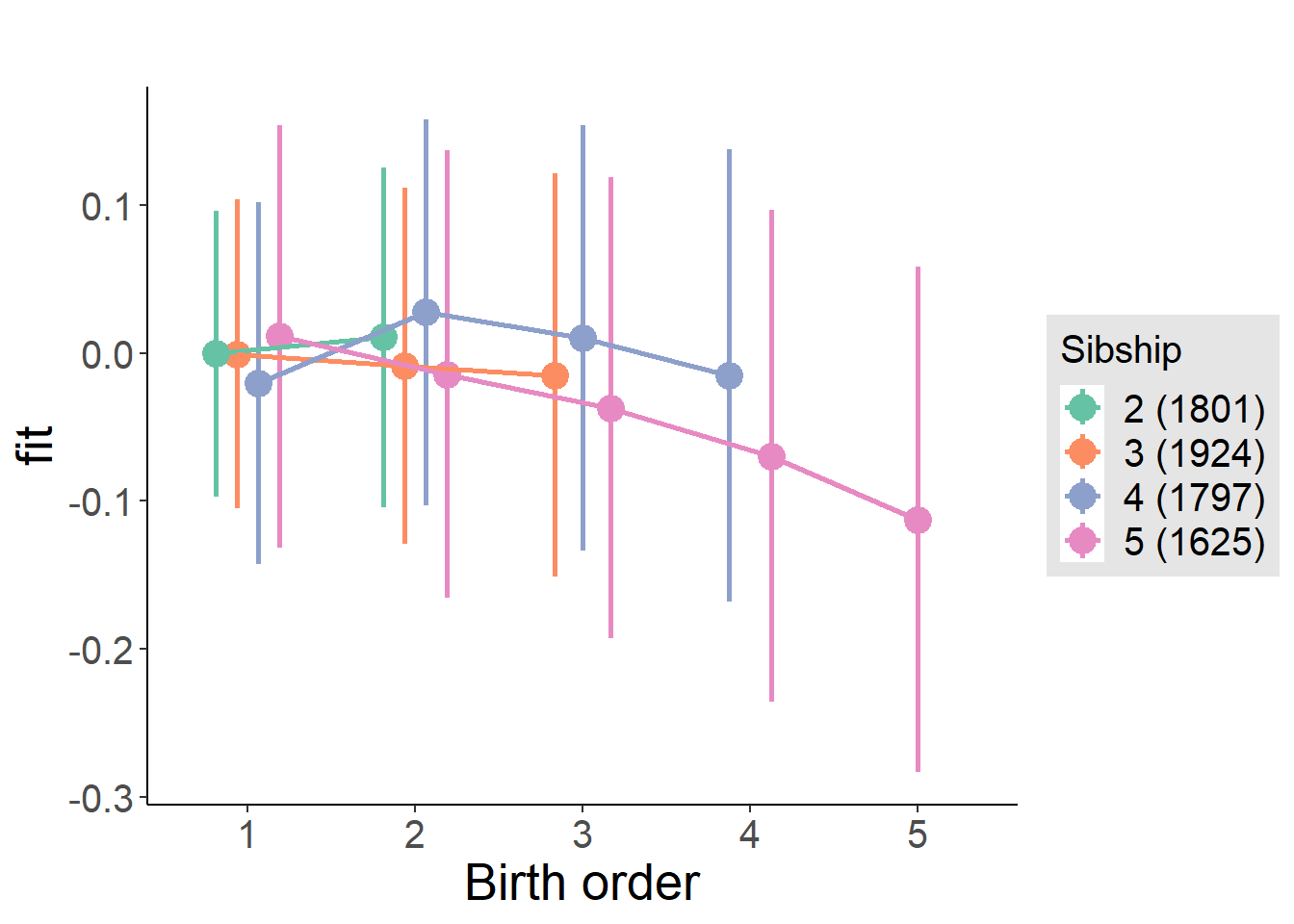
Model Comparison
###### Model 1 - Model 2
anova(m1_covariates_only, m2_birthorder_linear, m3_birthorder_nonlinear, m4_interaction)## refitting model(s) with ML (instead of REML)| Df | AIC | BIC | logLik | deviance | Chisq | Chi Df | Pr(>Chisq) |
|---|---|---|---|---|---|---|---|
| 10 | 20030 | 20099 | -10005 | 20010 | NA | NA | NA |
| 11 | 20031 | 20107 | -10005 | 20009 | 1.376 | 1 | 0.2407 |
| 14 | 20036 | 20132 | -10004 | 20008 | 1.405 | 3 | 0.7043 |
| 20 | 20046 | 20184 | -10003 | 20006 | 1.255 | 6 | 0.9741 |
Maternal birth order
outcome_uterus_m1 <- update(m2_birthorder_linear, data = birthorder %>%
mutate(sibling_count = sibling_count_uterus_alive_factor,
birth_order_nonlinear = birthorder_uterus_alive_factor,
birth_order = birthorder_uterus_alive,
count_birth_order = count_birthorder_uterus_alive) %>%
filter(sibling_count != "1"))
compare_models_markdown(outcome_uterus_m1)Basic Model
Model Summary
m1_covariates_only <- update(m2_birthorder_linear, formula = . ~ . - birth_order)
tidy(m1_covariates_only, conf.int = T, conf.level = 0.995)| effect | group | term | estimate | std.error | statistic | df | p.value | conf.low | conf.high |
|---|---|---|---|---|---|---|---|---|---|
| fixed | NA | (Intercept) | -0.772 | 0.5401 | -1.429 | 4500 | 0.153 | -2.288 | 0.7442 |
| fixed | NA | poly(age, 3, raw = TRUE)1 | 0.1448 | 0.06302 | 2.297 | 4497 | 0.02166 | -0.03214 | 0.3217 |
| fixed | NA | poly(age, 3, raw = TRUE)2 | -0.006181 | 0.002322 | -2.662 | 4492 | 0.007793 | -0.0127 | 0.0003365 |
| fixed | NA | poly(age, 3, raw = TRUE)3 | 0.00007284 | 0.0000272 | 2.678 | 4487 | 0.007428 | -0.000003503 | 0.0001492 |
| fixed | NA | male | -0.2789 | 0.02913 | -9.575 | 4471 | 1.642e-21 | -0.3607 | -0.1971 |
| fixed | NA | sibling_count3 | 0.01973 | 0.03929 | 0.5021 | 3297 | 0.6157 | -0.09056 | 0.13 |
| fixed | NA | sibling_count4 | 0.02189 | 0.0423 | 0.5175 | 2818 | 0.6048 | -0.09684 | 0.1406 |
| fixed | NA | sibling_count5 | 0.07225 | 0.04815 | 1.5 | 2435 | 0.1336 | -0.06292 | 0.2074 |
| ran_pars | mother_pidlink | sd__(Intercept) | 0.258 | NA | NA | NA | NA | NA | NA |
| ran_pars | Residual | sd__Observation | 0.9439 | NA | NA | NA | NA | NA | NA |
Coefficient Plot
plot(allEffects(m1_covariates_only, confidence.level = 0.995))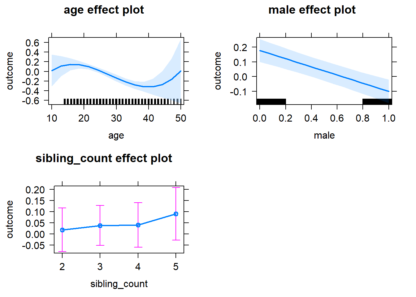
Add Birth Order Linear
Model Summary
tidy(m2_birthorder_linear, conf.int = T, conf.level = 0.995)| effect | group | term | estimate | std.error | statistic | df | p.value | conf.low | conf.high |
|---|---|---|---|---|---|---|---|---|---|
| fixed | NA | (Intercept) | -0.7391 | 0.5407 | -1.367 | 4498 | 0.1717 | -2.257 | 0.7787 |
| fixed | NA | birth_order | -0.01964 | 0.01533 | -1.281 | 4211 | 0.2002 | -0.06268 | 0.02339 |
| fixed | NA | poly(age, 3, raw = TRUE)1 | 0.1436 | 0.06302 | 2.278 | 4496 | 0.02275 | -0.03332 | 0.3205 |
| fixed | NA | poly(age, 3, raw = TRUE)2 | -0.006114 | 0.002322 | -2.633 | 4491 | 0.008494 | -0.01263 | 0.0004043 |
| fixed | NA | poly(age, 3, raw = TRUE)3 | 0.00007166 | 0.00002721 | 2.633 | 4486 | 0.008481 | -0.000004723 | 0.000148 |
| fixed | NA | male | -0.2782 | 0.02913 | -9.551 | 4470 | 2.053e-21 | -0.36 | -0.1965 |
| fixed | NA | sibling_count3 | 0.02871 | 0.0399 | 0.7195 | 3362 | 0.4719 | -0.0833 | 0.1407 |
| fixed | NA | sibling_count4 | 0.0425 | 0.04525 | 0.9393 | 3062 | 0.3476 | -0.08451 | 0.1695 |
| fixed | NA | sibling_count5 | 0.1068 | 0.05517 | 1.935 | 2979 | 0.05307 | -0.0481 | 0.2616 |
| ran_pars | mother_pidlink | sd__(Intercept) | 0.2574 | NA | NA | NA | NA | NA | NA |
| ran_pars | Residual | sd__Observation | 0.944 | NA | NA | NA | NA | NA | NA |
Coefficient Plot
plot_birthorder2(m2_birthorder_linear, separate = FALSE)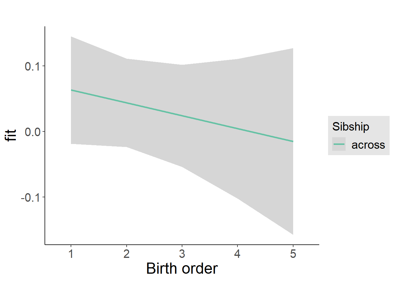
Add Birth Order Factor
Model Summary
m3_birthorder_nonlinear = update(m1_covariates_only, formula = . ~ . + birth_order_nonlinear)
tidy(m3_birthorder_nonlinear, conf.int = T, conf.level = 0.995)| effect | group | term | estimate | std.error | statistic | df | p.value | conf.low | conf.high |
|---|---|---|---|---|---|---|---|---|---|
| fixed | NA | (Intercept) | -0.802 | 0.5405 | -1.484 | 4494 | 0.138 | -2.319 | 0.7154 |
| fixed | NA | poly(age, 3, raw = TRUE)1 | 0.1487 | 0.06301 | 2.36 | 4491 | 0.01832 | -0.02817 | 0.3256 |
| fixed | NA | poly(age, 3, raw = TRUE)2 | -0.006297 | 0.002322 | -2.712 | 4486 | 0.006713 | -0.01281 | 0.0002206 |
| fixed | NA | poly(age, 3, raw = TRUE)3 | 0.00007357 | 0.0000272 | 2.704 | 4481 | 0.006867 | -0.00000279 | 0.0001499 |
| fixed | NA | male | -0.2775 | 0.02911 | -9.532 | 4467 | 2.461e-21 | -0.3592 | -0.1958 |
| fixed | NA | sibling_count3 | 0.003462 | 0.04052 | 0.08544 | 3492 | 0.9319 | -0.1103 | 0.1172 |
| fixed | NA | sibling_count4 | 0.03207 | 0.04591 | 0.6985 | 3173 | 0.4849 | -0.0968 | 0.1609 |
| fixed | NA | sibling_count5 | 0.1202 | 0.05608 | 2.143 | 3073 | 0.03215 | -0.03721 | 0.2776 |
| fixed | NA | birth_order_nonlinear2 | -0.01941 | 0.03488 | -0.5564 | 3660 | 0.578 | -0.1173 | 0.07849 |
| fixed | NA | birth_order_nonlinear3 | 0.07233 | 0.0444 | 1.629 | 3899 | 0.1034 | -0.05229 | 0.1969 |
| fixed | NA | birth_order_nonlinear4 | -0.1266 | 0.05955 | -2.127 | 4094 | 0.03351 | -0.2938 | 0.04052 |
| fixed | NA | birth_order_nonlinear5 | -0.1761 | 0.09279 | -1.898 | 3980 | 0.0578 | -0.4366 | 0.08437 |
| ran_pars | mother_pidlink | sd__(Intercept) | 0.2574 | NA | NA | NA | NA | NA | NA |
| ran_pars | Residual | sd__Observation | 0.943 | NA | NA | NA | NA | NA | NA |
Coefficient Plot
plot_birthorder(m3_birthorder_nonlinear, separate = FALSE)
Add Interaction
Model Summary
m4_interaction = update(m3_birthorder_nonlinear, formula = . ~ . - birth_order_nonlinear - sibling_count + count_birth_order)
tidy(m4_interaction, conf.int = T, conf.level = 0.995)| effect | group | term | estimate | std.error | statistic | df | p.value | conf.low | conf.high |
|---|---|---|---|---|---|---|---|---|---|
| fixed | NA | (Intercept) | -0.8205 | 0.5404 | -1.518 | 4488 | 0.129 | -2.337 | 0.6963 |
| fixed | NA | poly(age, 3, raw = TRUE)1 | 0.151 | 0.063 | 2.396 | 4486 | 0.0166 | -0.02587 | 0.3278 |
| fixed | NA | poly(age, 3, raw = TRUE)2 | -0.006352 | 0.002321 | -2.736 | 4481 | 0.006236 | -0.01287 | 0.000164 |
| fixed | NA | poly(age, 3, raw = TRUE)3 | 0.0000739 | 0.0000272 | 2.717 | 4476 | 0.006621 | -0.00000246 | 0.0001503 |
| fixed | NA | male | -0.2777 | 0.0291 | -9.54 | 4459 | 2.277e-21 | -0.3594 | -0.196 |
| fixed | NA | count_birth_order2/2 | -0.03788 | 0.05976 | -0.6339 | 3814 | 0.5262 | -0.2056 | 0.1299 |
| fixed | NA | count_birth_order1/3 | -0.04035 | 0.05236 | -0.7706 | 4486 | 0.441 | -0.1873 | 0.1066 |
| fixed | NA | count_birth_order2/3 | 0.0175 | 0.05722 | 0.3057 | 4490 | 0.7598 | -0.1431 | 0.1781 |
| fixed | NA | count_birth_order3/3 | 0.08657 | 0.06399 | 1.353 | 4487 | 0.1762 | -0.09306 | 0.2662 |
| fixed | NA | count_birth_order1/4 | 0.04223 | 0.06424 | 0.6574 | 4487 | 0.511 | -0.1381 | 0.2226 |
| fixed | NA | count_birth_order2/4 | 0.04556 | 0.06641 | 0.6861 | 4490 | 0.4927 | -0.1408 | 0.232 |
| fixed | NA | count_birth_order3/4 | 0.0414 | 0.07016 | 0.59 | 4482 | 0.5552 | -0.1555 | 0.2383 |
| fixed | NA | count_birth_order4/4 | -0.1137 | 0.07288 | -1.56 | 4480 | 0.1188 | -0.3183 | 0.09089 |
| fixed | NA | count_birth_order1/5 | 0.205 | 0.08742 | 2.345 | 4489 | 0.01907 | -0.0404 | 0.4504 |
| fixed | NA | count_birth_order2/5 | -0.1068 | 0.09339 | -1.144 | 4481 | 0.2529 | -0.3689 | 0.1553 |
| fixed | NA | count_birth_order3/5 | 0.2462 | 0.0875 | 2.814 | 4476 | 0.004913 | 0.0006185 | 0.4918 |
| fixed | NA | count_birth_order4/5 | 0.004021 | 0.08424 | 0.04773 | 4477 | 0.9619 | -0.2324 | 0.2405 |
| fixed | NA | count_birth_order5/5 | -0.06247 | 0.08762 | -0.7129 | 4469 | 0.4759 | -0.3084 | 0.1835 |
| ran_pars | mother_pidlink | sd__(Intercept) | 0.259 | NA | NA | NA | NA | NA | NA |
| ran_pars | Residual | sd__Observation | 0.942 | NA | NA | NA | NA | NA | NA |
Coefficient Plot
plot_birthorder(m4_interaction)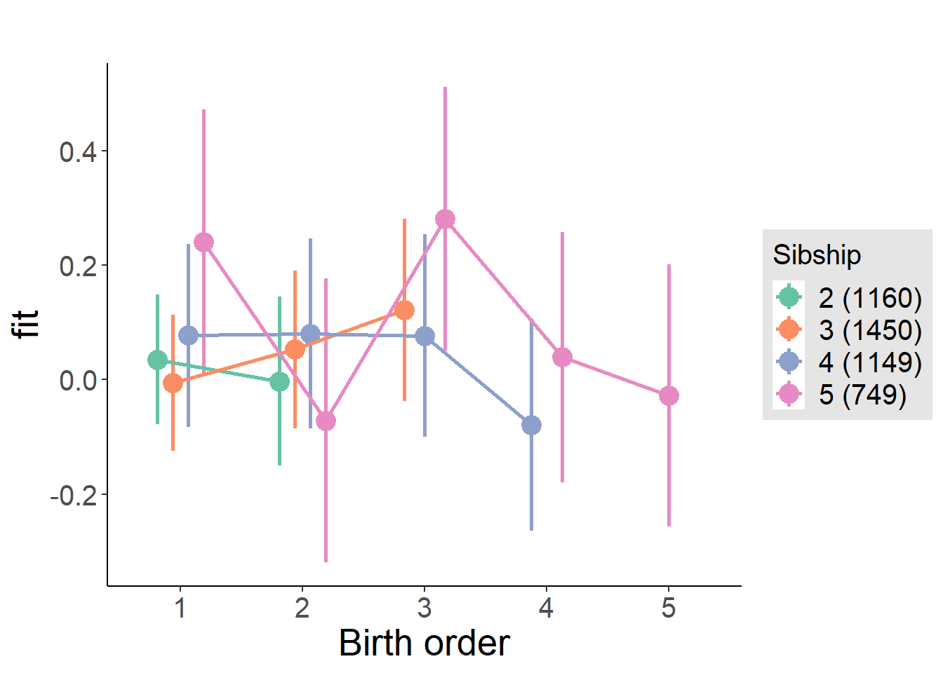
Model Comparison
###### Model 1 - Model 2
anova(m1_covariates_only, m2_birthorder_linear, m3_birthorder_nonlinear, m4_interaction)## refitting model(s) with ML (instead of REML)| Df | AIC | BIC | logLik | deviance | Chisq | Chi Df | Pr(>Chisq) |
|---|---|---|---|---|---|---|---|
| 10 | 12601 | 12665 | -6290 | 12581 | NA | NA | NA |
| 11 | 12601 | 12672 | -6290 | 12579 | 1.645 | 1 | 0.1996 |
| 14 | 12595 | 12685 | -6284 | 12567 | 12.18 | 3 | 0.006797 |
| 20 | 12596 | 12724 | -6278 | 12556 | 11.23 | 6 | 0.08139 |
Maternal pregnancy order
outcome_preg_m1 <- update(m2_birthorder_linear, data = birthorder %>%
mutate(sibling_count = sibling_count_uterus_preg_factor,
birth_order_nonlinear = birthorder_uterus_preg_factor,
birth_order = birthorder_uterus_preg,
count_birth_order = count_birthorder_uterus_preg
) %>%
filter(sibling_count != "1"))
compare_models_markdown(outcome_preg_m1)Basic Model
Model Summary
m1_covariates_only <- update(m2_birthorder_linear, formula = . ~ . - birth_order)
tidy(m1_covariates_only, conf.int = T, conf.level = 0.995)| effect | group | term | estimate | std.error | statistic | df | p.value | conf.low | conf.high |
|---|---|---|---|---|---|---|---|---|---|
| fixed | NA | (Intercept) | -1.064 | 0.5549 | -1.918 | 4177 | 0.05516 | -2.622 | 0.4933 |
| fixed | NA | poly(age, 3, raw = TRUE)1 | 0.1824 | 0.0648 | 2.815 | 4174 | 0.0049 | 0.0005176 | 0.3643 |
| fixed | NA | poly(age, 3, raw = TRUE)2 | -0.007538 | 0.002388 | -3.156 | 4170 | 0.001609 | -0.01424 | -0.0008341 |
| fixed | NA | poly(age, 3, raw = TRUE)3 | 0.00008825 | 0.00002798 | 3.154 | 4165 | 0.00162 | 0.000009715 | 0.0001668 |
| fixed | NA | male | -0.3028 | 0.03018 | -10.03 | 4149 | 1.982e-23 | -0.3875 | -0.2181 |
| fixed | NA | sibling_count3 | 0.000532 | 0.04237 | 0.01256 | 3145 | 0.99 | -0.1184 | 0.1195 |
| fixed | NA | sibling_count4 | 0.002049 | 0.0447 | 0.04585 | 2809 | 0.9634 | -0.1234 | 0.1275 |
| fixed | NA | sibling_count5 | -0.03458 | 0.04774 | -0.7244 | 2443 | 0.4689 | -0.1686 | 0.09943 |
| ran_pars | mother_pidlink | sd__(Intercept) | 0.2497 | NA | NA | NA | NA | NA | NA |
| ran_pars | Residual | sd__Observation | 0.9434 | NA | NA | NA | NA | NA | NA |
Coefficient Plot
plot(allEffects(m1_covariates_only, confidence.level = 0.995))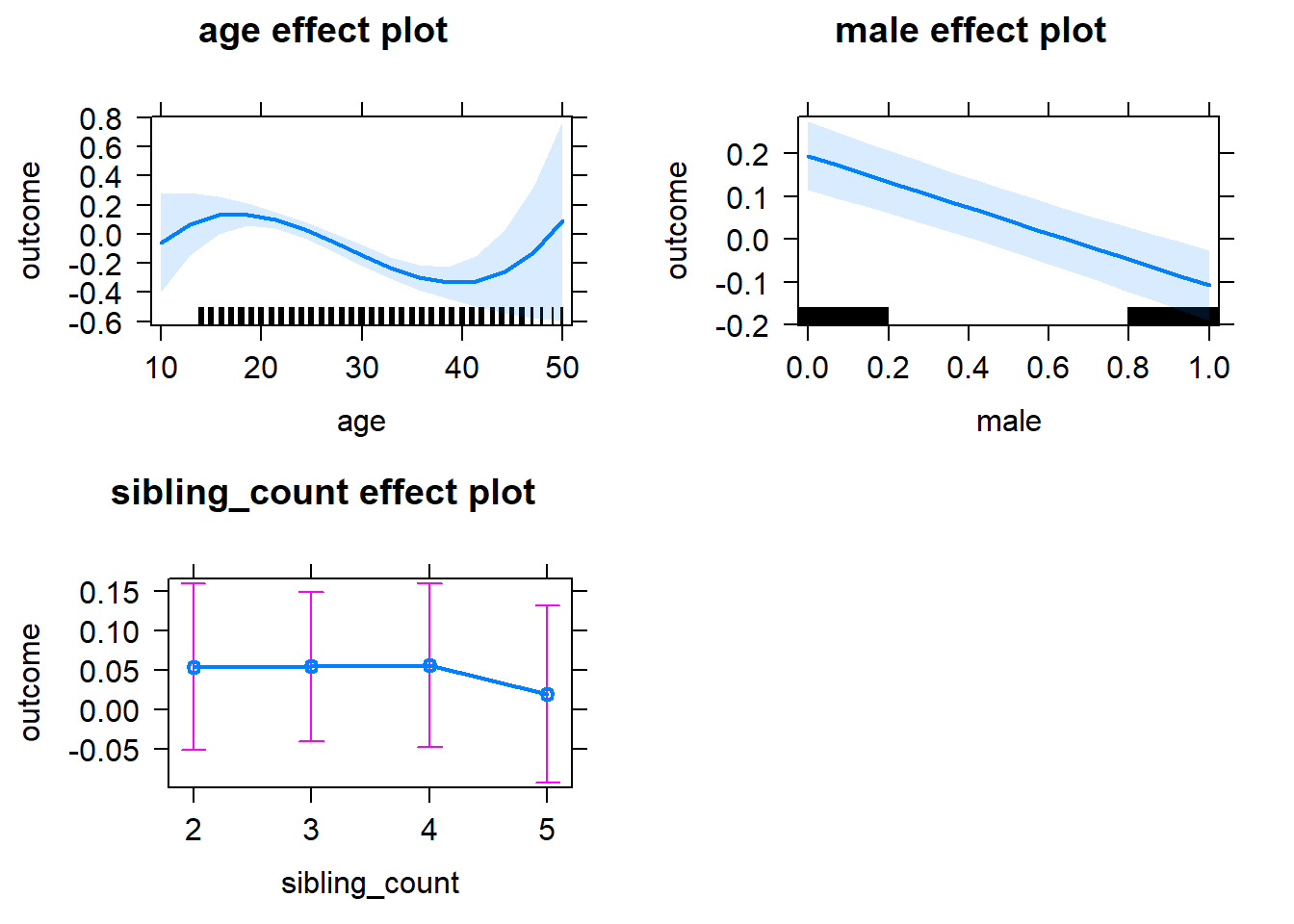
Add Birth Order Linear
Model Summary
tidy(m2_birthorder_linear, conf.int = T, conf.level = 0.995)| effect | group | term | estimate | std.error | statistic | df | p.value | conf.low | conf.high |
|---|---|---|---|---|---|---|---|---|---|
| fixed | NA | (Intercept) | -1.035 | 0.5555 | -1.863 | 4176 | 0.06258 | -2.594 | 0.5246 |
| fixed | NA | birth_order | -0.01807 | 0.01533 | -1.179 | 3985 | 0.2385 | -0.06109 | 0.02495 |
| fixed | NA | poly(age, 3, raw = TRUE)1 | 0.1815 | 0.0648 | 2.8 | 4173 | 0.005133 | -0.0004529 | 0.3634 |
| fixed | NA | poly(age, 3, raw = TRUE)2 | -0.007482 | 0.002389 | -3.132 | 4169 | 0.001746 | -0.01419 | -0.0007773 |
| fixed | NA | poly(age, 3, raw = TRUE)3 | 0.00008723 | 0.00002799 | 3.117 | 4165 | 0.001842 | 0.000008663 | 0.0001658 |
| fixed | NA | male | -0.3024 | 0.03018 | -10.02 | 4148 | 2.269e-23 | -0.3871 | -0.2177 |
| fixed | NA | sibling_count3 | 0.008793 | 0.04294 | 0.2048 | 3190 | 0.8377 | -0.1117 | 0.1293 |
| fixed | NA | sibling_count4 | 0.02037 | 0.04731 | 0.4305 | 2987 | 0.6669 | -0.1124 | 0.1532 |
| fixed | NA | sibling_count5 | -0.005312 | 0.05381 | -0.09872 | 2865 | 0.9214 | -0.1564 | 0.1457 |
| ran_pars | mother_pidlink | sd__(Intercept) | 0.2487 | NA | NA | NA | NA | NA | NA |
| ran_pars | Residual | sd__Observation | 0.9437 | NA | NA | NA | NA | NA | NA |
Coefficient Plot
plot_birthorder2(m2_birthorder_linear, separate = FALSE)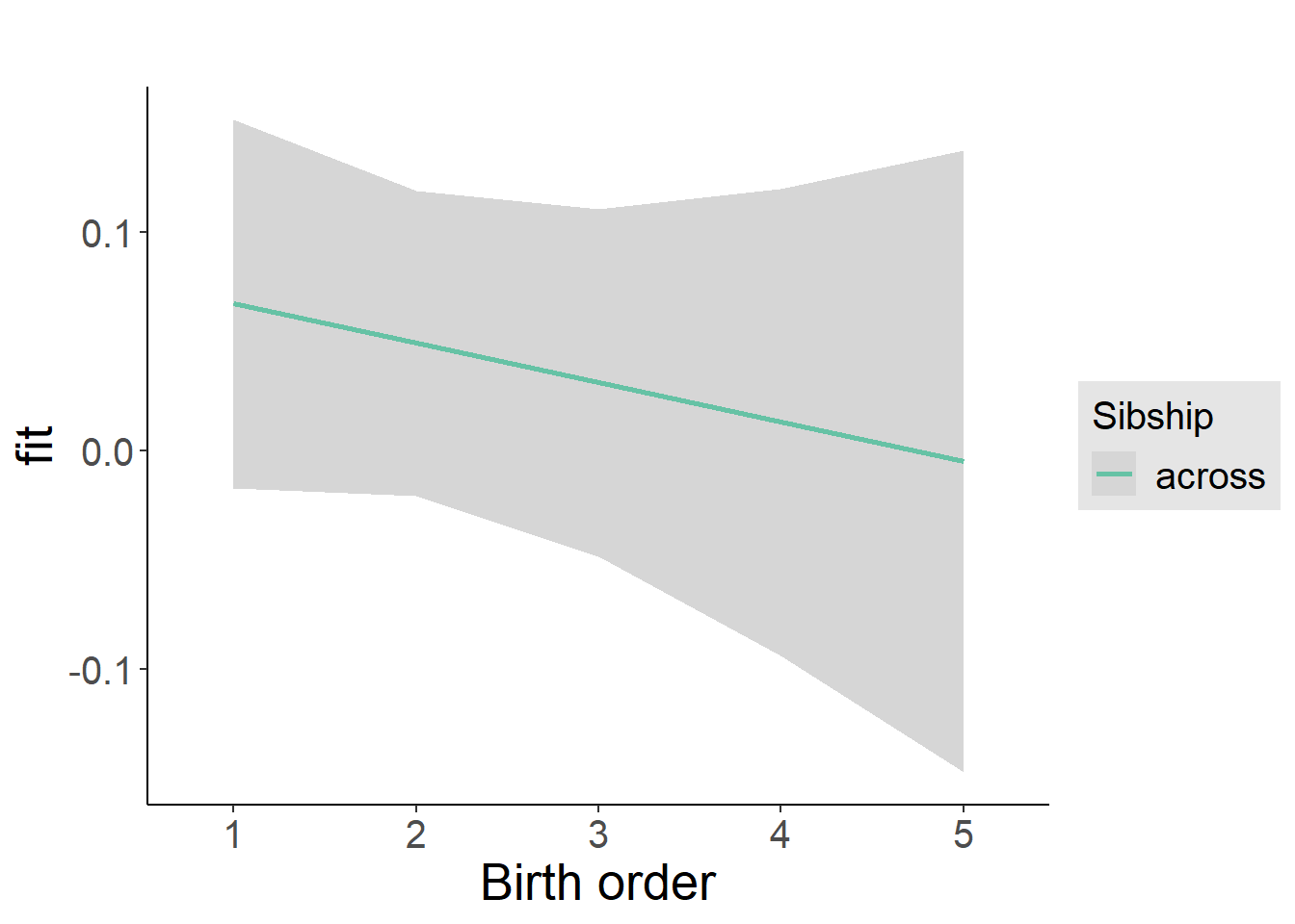
Add Birth Order Factor
Model Summary
m3_birthorder_nonlinear = update(m1_covariates_only, formula = . ~ . + birth_order_nonlinear)
tidy(m3_birthorder_nonlinear, conf.int = T, conf.level = 0.995)| effect | group | term | estimate | std.error | statistic | df | p.value | conf.low | conf.high |
|---|---|---|---|---|---|---|---|---|---|
| fixed | NA | (Intercept) | -1.099 | 0.5551 | -1.98 | 4171 | 0.04777 | -2.657 | 0.4591 |
| fixed | NA | poly(age, 3, raw = TRUE)1 | 0.1871 | 0.06476 | 2.888 | 4169 | 0.003894 | 0.005257 | 0.3689 |
| fixed | NA | poly(age, 3, raw = TRUE)2 | -0.007687 | 0.002387 | -3.22 | 4164 | 0.001292 | -0.01439 | -0.0009859 |
| fixed | NA | poly(age, 3, raw = TRUE)3 | 0.00008946 | 0.00002797 | 3.198 | 4159 | 0.001392 | 0.00001095 | 0.000168 |
| fixed | NA | male | -0.3027 | 0.03014 | -10.04 | 4144 | 1.816e-23 | -0.3873 | -0.2181 |
| fixed | NA | sibling_count3 | -0.01704 | 0.04356 | -0.3911 | 3296 | 0.6957 | -0.1393 | 0.1052 |
| fixed | NA | sibling_count4 | -0.002756 | 0.04797 | -0.05745 | 3083 | 0.9542 | -0.1374 | 0.1319 |
| fixed | NA | sibling_count5 | 0.006124 | 0.05433 | 0.1127 | 2915 | 0.9103 | -0.1464 | 0.1586 |
| fixed | NA | birth_order_nonlinear2 | -0.01769 | 0.03621 | -0.4886 | 3448 | 0.6252 | -0.1193 | 0.08396 |
| fixed | NA | birth_order_nonlinear3 | 0.07904 | 0.04572 | 1.729 | 3689 | 0.08396 | -0.04931 | 0.2074 |
| fixed | NA | birth_order_nonlinear4 | -0.05703 | 0.06045 | -0.9435 | 3847 | 0.3455 | -0.2267 | 0.1127 |
| fixed | NA | birth_order_nonlinear5 | -0.2522 | 0.08864 | -2.846 | 3761 | 0.004457 | -0.5011 | -0.003418 |
| ran_pars | mother_pidlink | sd__(Intercept) | 0.2513 | NA | NA | NA | NA | NA | NA |
| ran_pars | Residual | sd__Observation | 0.9417 | NA | NA | NA | NA | NA | NA |
Coefficient Plot
plot_birthorder(m3_birthorder_nonlinear, separate = FALSE)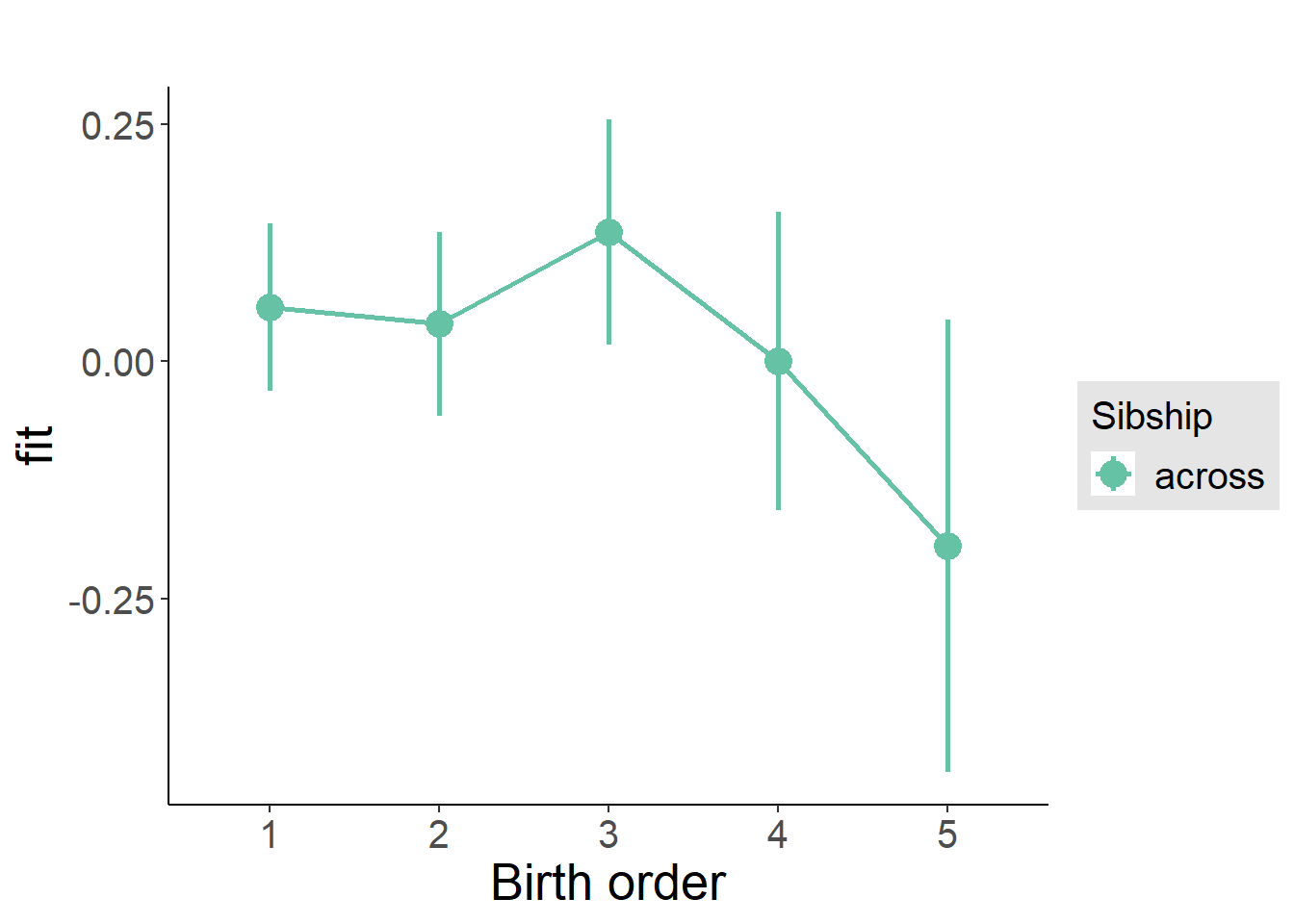
Add Interaction
Model Summary
m4_interaction = update(m3_birthorder_nonlinear, formula = . ~ . - birth_order_nonlinear - sibling_count + count_birth_order)
tidy(m4_interaction, conf.int = T, conf.level = 0.995)| effect | group | term | estimate | std.error | statistic | df | p.value | conf.low | conf.high |
|---|---|---|---|---|---|---|---|---|---|
| fixed | NA | (Intercept) | -1.073 | 0.5554 | -1.932 | 4165 | 0.05337 | -2.632 | 0.4858 |
| fixed | NA | poly(age, 3, raw = TRUE)1 | 0.1835 | 0.06479 | 2.832 | 4163 | 0.004652 | 0.001599 | 0.3653 |
| fixed | NA | poly(age, 3, raw = TRUE)2 | -0.007532 | 0.002388 | -3.154 | 4158 | 0.001624 | -0.01424 | -0.000828 |
| fixed | NA | poly(age, 3, raw = TRUE)3 | 0.0000874 | 0.00002799 | 3.122 | 4153 | 0.001806 | 0.000008829 | 0.000166 |
| fixed | NA | male | -0.304 | 0.03016 | -10.08 | 4139 | 1.29e-23 | -0.3887 | -0.2193 |
| fixed | NA | count_birth_order2/2 | -0.01504 | 0.06528 | -0.2304 | 3580 | 0.8178 | -0.1983 | 0.1682 |
| fixed | NA | count_birth_order1/3 | -0.02606 | 0.05658 | -0.4606 | 4164 | 0.6451 | -0.1849 | 0.1328 |
| fixed | NA | count_birth_order2/3 | -0.03837 | 0.06136 | -0.6253 | 4167 | 0.5318 | -0.2106 | 0.1339 |
| fixed | NA | count_birth_order3/3 | 0.08944 | 0.06909 | 1.295 | 4164 | 0.1955 | -0.1045 | 0.2834 |
| fixed | NA | count_birth_order1/4 | -0.05097 | 0.06716 | -0.7588 | 4165 | 0.448 | -0.2395 | 0.1376 |
| fixed | NA | count_birth_order2/4 | -0.00024 | 0.06836 | -0.003511 | 4167 | 0.9972 | -0.1921 | 0.1917 |
| fixed | NA | count_birth_order3/4 | 0.1025 | 0.07499 | 1.367 | 4160 | 0.1716 | -0.108 | 0.313 |
| fixed | NA | count_birth_order4/4 | -0.03813 | 0.07724 | -0.4936 | 4159 | 0.6216 | -0.2549 | 0.1787 |
| fixed | NA | count_birth_order1/5 | 0.1186 | 0.07992 | 1.484 | 4167 | 0.1378 | -0.1057 | 0.343 |
| fixed | NA | count_birth_order2/5 | -0.03846 | 0.08565 | -0.449 | 4164 | 0.6535 | -0.2789 | 0.202 |
| fixed | NA | count_birth_order3/5 | 0.0095 | 0.0832 | 0.1142 | 4160 | 0.9091 | -0.224 | 0.243 |
| fixed | NA | count_birth_order4/5 | -0.07809 | 0.08619 | -0.9059 | 4151 | 0.365 | -0.32 | 0.1639 |
| fixed | NA | count_birth_order5/5 | -0.2462 | 0.08636 | -2.851 | 4147 | 0.004375 | -0.4887 | -0.003826 |
| ran_pars | mother_pidlink | sd__(Intercept) | 0.2471 | NA | NA | NA | NA | NA | NA |
| ran_pars | Residual | sd__Observation | 0.9428 | NA | NA | NA | NA | NA | NA |
Coefficient Plot
plot_birthorder(m4_interaction)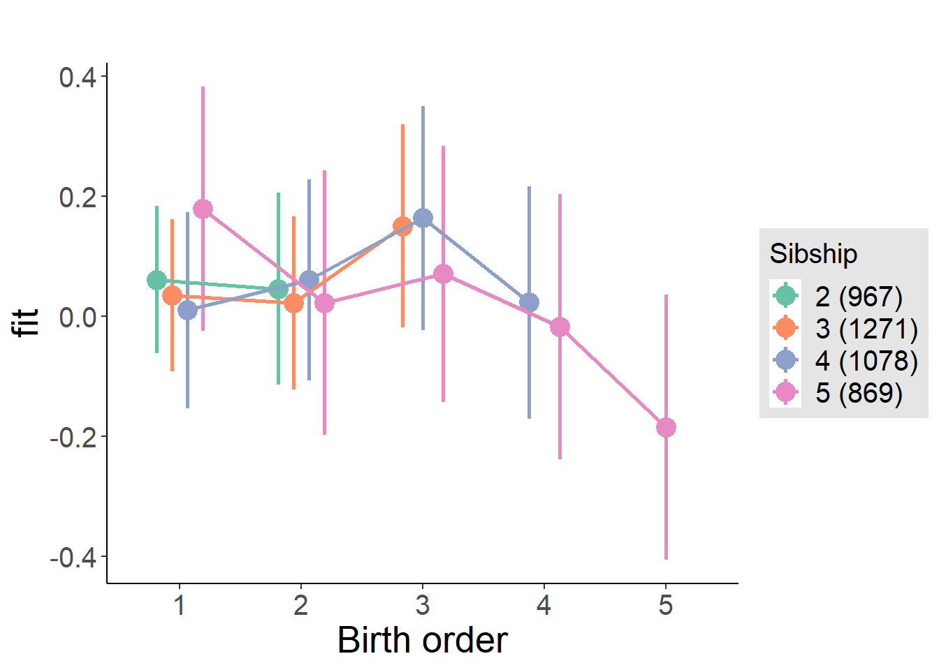
Model Comparison
###### Model 1 - Model 2
anova(m1_covariates_only, m2_birthorder_linear, m3_birthorder_nonlinear, m4_interaction)## refitting model(s) with ML (instead of REML)| Df | AIC | BIC | logLik | deviance | Chisq | Chi Df | Pr(>Chisq) |
|---|---|---|---|---|---|---|---|
| 10 | 11678 | 11741 | -5829 | 11658 | NA | NA | NA |
| 11 | 11679 | 11748 | -5828 | 11657 | 1.394 | 1 | 0.2378 |
| 14 | 11671 | 11759 | -5821 | 11643 | 13.85 | 3 | 0.003115 |
| 20 | 11677 | 11804 | -5819 | 11637 | 5.612 | 6 | 0.468 |
Parental full sibling order
outcome_parental_m1 <- update(m2_birthorder_linear, data = birthorder %>%
mutate(sibling_count = sibling_count_genes_factor,
birth_order_nonlinear = birthorder_genes_factor,
birth_order = birthorder_genes,
count_birth_order = count_birthorder_genes
) %>%
filter(sibling_count != "1"))
compare_models_markdown(outcome_parental_m1)Basic Model
Model Summary
m1_covariates_only <- update(m2_birthorder_linear, formula = . ~ . - birth_order)
tidy(m1_covariates_only, conf.int = T, conf.level = 0.995)| effect | group | term | estimate | std.error | statistic | df | p.value | conf.low | conf.high |
|---|---|---|---|---|---|---|---|---|---|
| fixed | NA | (Intercept) | -0.9207 | 0.5436 | -1.694 | 4484 | 0.09038 | -2.447 | 0.6052 |
| fixed | NA | poly(age, 3, raw = TRUE)1 | 0.1625 | 0.06351 | 2.558 | 4480 | 0.01055 | -0.0158 | 0.3407 |
| fixed | NA | poly(age, 3, raw = TRUE)2 | -0.006881 | 0.002343 | -2.937 | 4474 | 0.003335 | -0.01346 | -0.0003037 |
| fixed | NA | poly(age, 3, raw = TRUE)3 | 0.00008168 | 0.0000275 | 2.97 | 4468 | 0.002991 | 0.00000449 | 0.0001589 |
| fixed | NA | male | -0.2813 | 0.02911 | -9.664 | 4461 | 7.035e-22 | -0.3631 | -0.1996 |
| fixed | NA | sibling_count3 | 0.02414 | 0.0386 | 0.6253 | 3261 | 0.5318 | -0.08423 | 0.1325 |
| fixed | NA | sibling_count4 | 0.02711 | 0.04178 | 0.6489 | 2789 | 0.5165 | -0.09016 | 0.1444 |
| fixed | NA | sibling_count5 | 0.063 | 0.04901 | 1.285 | 2296 | 0.1988 | -0.07458 | 0.2006 |
| ran_pars | mother_pidlink | sd__(Intercept) | 0.2432 | NA | NA | NA | NA | NA | NA |
| ran_pars | Residual | sd__Observation | 0.9447 | NA | NA | NA | NA | NA | NA |
Coefficient Plot
plot(allEffects(m1_covariates_only, confidence.level = 0.995))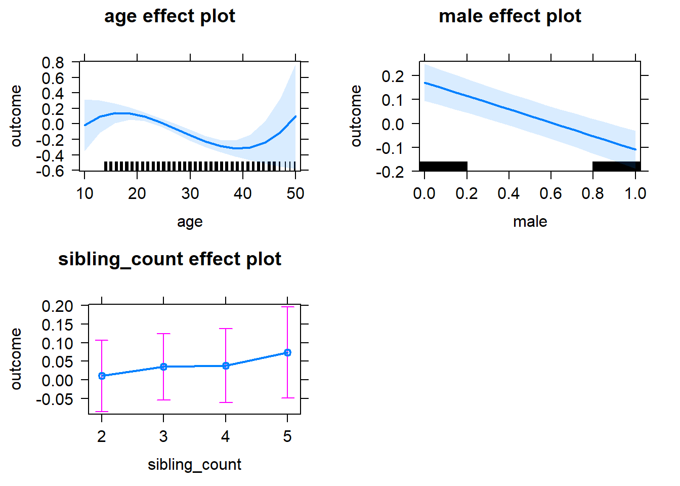
Add Birth Order Linear
Model Summary
tidy(m2_birthorder_linear, conf.int = T, conf.level = 0.995)| effect | group | term | estimate | std.error | statistic | df | p.value | conf.low | conf.high |
|---|---|---|---|---|---|---|---|---|---|
| fixed | NA | (Intercept) | -0.8966 | 0.5442 | -1.647 | 4483 | 0.09954 | -2.424 | 0.6311 |
| fixed | NA | birth_order | -0.0148 | 0.01551 | -0.9544 | 4187 | 0.3399 | -0.05834 | 0.02873 |
| fixed | NA | poly(age, 3, raw = TRUE)1 | 0.1617 | 0.06351 | 2.545 | 4479 | 0.01095 | -0.01661 | 0.34 |
| fixed | NA | poly(age, 3, raw = TRUE)2 | -0.006834 | 0.002344 | -2.916 | 4473 | 0.003563 | -0.01341 | -0.0002554 |
| fixed | NA | poly(age, 3, raw = TRUE)3 | 0.00008083 | 0.00002751 | 2.938 | 4467 | 0.003321 | 0.000003602 | 0.0001581 |
| fixed | NA | male | -0.2809 | 0.02912 | -9.649 | 4460 | 8.13e-22 | -0.3627 | -0.1992 |
| fixed | NA | sibling_count3 | 0.03089 | 0.03924 | 0.7871 | 3323 | 0.4313 | -0.07927 | 0.141 |
| fixed | NA | sibling_count4 | 0.04257 | 0.04481 | 0.9501 | 3049 | 0.3421 | -0.0832 | 0.1683 |
| fixed | NA | sibling_count5 | 0.08778 | 0.05546 | 1.583 | 2789 | 0.1136 | -0.0679 | 0.2435 |
| ran_pars | mother_pidlink | sd__(Intercept) | 0.2424 | NA | NA | NA | NA | NA | NA |
| ran_pars | Residual | sd__Observation | 0.9449 | NA | NA | NA | NA | NA | NA |
Coefficient Plot
plot_birthorder2(m2_birthorder_linear, separate = FALSE)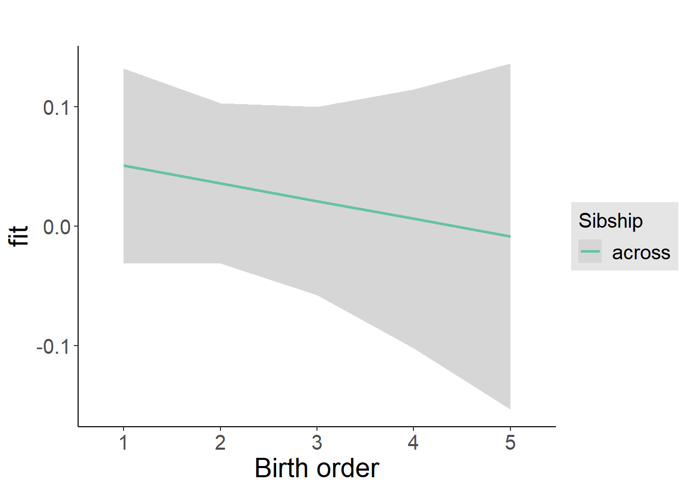
Add Birth Order Factor
Model Summary
m3_birthorder_nonlinear = update(m1_covariates_only, formula = . ~ . + birth_order_nonlinear)
tidy(m3_birthorder_nonlinear, conf.int = T, conf.level = 0.995)| effect | group | term | estimate | std.error | statistic | df | p.value | conf.low | conf.high |
|---|---|---|---|---|---|---|---|---|---|
| fixed | NA | (Intercept) | -0.9606 | 0.5441 | -1.765 | 4477 | 0.07755 | -2.488 | 0.5667 |
| fixed | NA | poly(age, 3, raw = TRUE)1 | 0.1673 | 0.06352 | 2.634 | 4473 | 0.008464 | -0.01098 | 0.3456 |
| fixed | NA | poly(age, 3, raw = TRUE)2 | -0.007035 | 0.002344 | -3.002 | 4467 | 0.0027 | -0.01361 | -0.0004562 |
| fixed | NA | poly(age, 3, raw = TRUE)3 | 0.00008295 | 0.00002751 | 3.016 | 4461 | 0.00258 | 0.000005735 | 0.0001602 |
| fixed | NA | male | -0.2791 | 0.0291 | -9.591 | 4457 | 1.407e-21 | -0.3608 | -0.1974 |
| fixed | NA | sibling_count3 | 0.007852 | 0.03989 | 0.1969 | 3462 | 0.8439 | -0.1041 | 0.1198 |
| fixed | NA | sibling_count4 | 0.03562 | 0.04548 | 0.7832 | 3163 | 0.4335 | -0.09204 | 0.1633 |
| fixed | NA | sibling_count5 | 0.102 | 0.05658 | 1.803 | 2890 | 0.07154 | -0.05683 | 0.2608 |
| fixed | NA | birth_order_nonlinear2 | -0.01212 | 0.03465 | -0.3497 | 3650 | 0.7266 | -0.1094 | 0.08515 |
| fixed | NA | birth_order_nonlinear3 | 0.06997 | 0.04421 | 1.583 | 3867 | 0.1136 | -0.05414 | 0.1941 |
| fixed | NA | birth_order_nonlinear4 | -0.1202 | 0.06077 | -1.978 | 4077 | 0.04798 | -0.2908 | 0.05037 |
| fixed | NA | birth_order_nonlinear5 | -0.1434 | 0.09921 | -1.446 | 4044 | 0.1483 | -0.4219 | 0.1351 |
| ran_pars | mother_pidlink | sd__(Intercept) | 0.241 | NA | NA | NA | NA | NA | NA |
| ran_pars | Residual | sd__Observation | 0.9444 | NA | NA | NA | NA | NA | NA |
Coefficient Plot
plot_birthorder(m3_birthorder_nonlinear, separate = FALSE)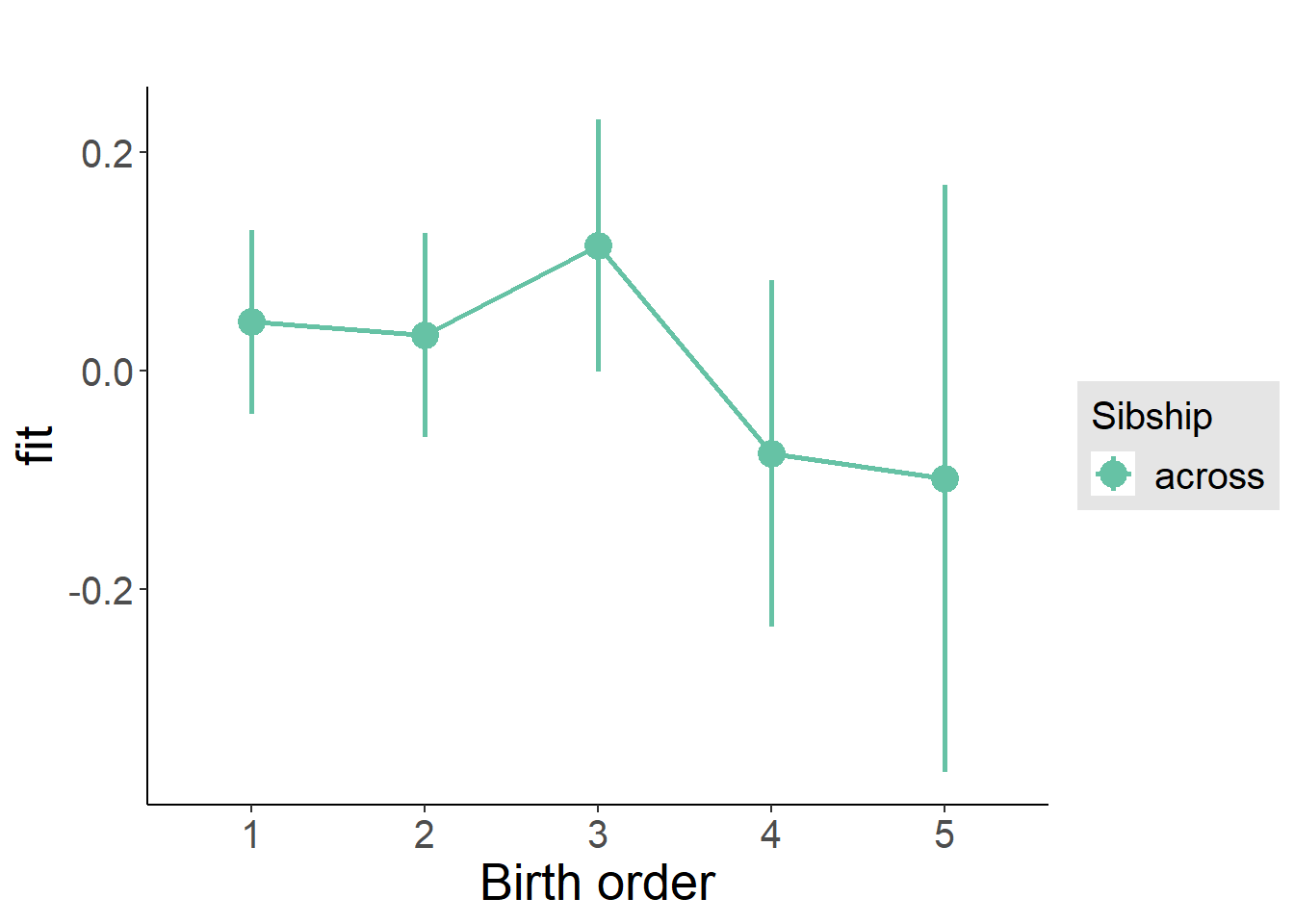
Add Interaction
Model Summary
m4_interaction = update(m3_birthorder_nonlinear, formula = . ~ . - birth_order_nonlinear - sibling_count + count_birth_order)
tidy(m4_interaction, conf.int = T, conf.level = 0.995)| effect | group | term | estimate | std.error | statistic | df | p.value | conf.low | conf.high |
|---|---|---|---|---|---|---|---|---|---|
| fixed | NA | (Intercept) | -0.9636 | 0.5441 | -1.771 | 4472 | 0.07661 | -2.491 | 0.5636 |
| fixed | NA | poly(age, 3, raw = TRUE)1 | 0.1681 | 0.06352 | 2.647 | 4468 | 0.008147 | -0.01016 | 0.3464 |
| fixed | NA | poly(age, 3, raw = TRUE)2 | -0.007048 | 0.002344 | -3.007 | 4462 | 0.002649 | -0.01363 | -0.0004697 |
| fixed | NA | poly(age, 3, raw = TRUE)3 | 0.00008295 | 0.00002751 | 3.015 | 4457 | 0.002585 | 0.000005721 | 0.0001602 |
| fixed | NA | male | -0.2786 | 0.0291 | -9.573 | 4450 | 1.676e-21 | -0.3603 | -0.1969 |
| fixed | NA | count_birth_order2/2 | -0.03536 | 0.05818 | -0.6078 | 3774 | 0.5434 | -0.1987 | 0.128 |
| fixed | NA | count_birth_order1/3 | -0.03386 | 0.0516 | -0.6561 | 4471 | 0.5118 | -0.1787 | 0.111 |
| fixed | NA | count_birth_order2/3 | 0.02379 | 0.05707 | 0.4168 | 4475 | 0.6768 | -0.1364 | 0.184 |
| fixed | NA | count_birth_order3/3 | 0.08574 | 0.06273 | 1.367 | 4471 | 0.1718 | -0.09035 | 0.2618 |
| fixed | NA | count_birth_order1/4 | 0.03541 | 0.06439 | 0.5499 | 4473 | 0.5824 | -0.1453 | 0.2162 |
| fixed | NA | count_birth_order2/4 | 0.05524 | 0.06615 | 0.8351 | 4475 | 0.4037 | -0.1304 | 0.2409 |
| fixed | NA | count_birth_order3/4 | 0.06876 | 0.06929 | 0.9923 | 4467 | 0.3211 | -0.1257 | 0.2632 |
| fixed | NA | count_birth_order4/4 | -0.125 | 0.0732 | -1.707 | 4464 | 0.08782 | -0.3304 | 0.08049 |
| fixed | NA | count_birth_order1/5 | 0.1799 | 0.08702 | 2.067 | 4475 | 0.0388 | -0.06441 | 0.4241 |
| fixed | NA | count_birth_order2/5 | -0.1064 | 0.09603 | -1.108 | 4468 | 0.2679 | -0.376 | 0.1632 |
| fixed | NA | count_birth_order3/5 | 0.1785 | 0.09152 | 1.95 | 4462 | 0.05125 | -0.07845 | 0.4354 |
| fixed | NA | count_birth_order4/5 | 0.02266 | 0.08813 | 0.2571 | 4464 | 0.7971 | -0.2247 | 0.2701 |
| fixed | NA | count_birth_order5/5 | -0.04992 | 0.09361 | -0.5333 | 4458 | 0.5939 | -0.3127 | 0.2128 |
| ran_pars | mother_pidlink | sd__(Intercept) | 0.2413 | NA | NA | NA | NA | NA | NA |
| ran_pars | Residual | sd__Observation | 0.944 | NA | NA | NA | NA | NA | NA |
Coefficient Plot
plot_birthorder(m4_interaction)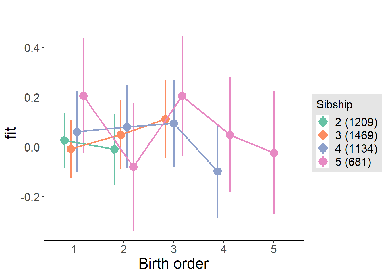
Model Comparison
###### Model 1 - Model 2
anova(m1_covariates_only, m2_birthorder_linear, m3_birthorder_nonlinear, m4_interaction)## refitting model(s) with ML (instead of REML)| Df | AIC | BIC | logLik | deviance | Chisq | Chi Df | Pr(>Chisq) |
|---|---|---|---|---|---|---|---|
| 10 | 12533 | 12597 | -6256 | 12513 | NA | NA | NA |
| 11 | 12534 | 12604 | -6256 | 12512 | 0.9136 | 1 | 0.3392 |
| 14 | 12530 | 12619 | -6251 | 12502 | 10.13 | 3 | 0.01746 |
| 20 | 12533 | 12661 | -6246 | 12493 | 9.021 | 6 | 0.1724 |
Compare birth order specifications
library(coefplot)
multiplot(outcome_naive_m1, outcome_preg_m1, outcome_uterus_m1, outcome_parental_m1, dodgeHeight = 0.6,
intercept = FALSE)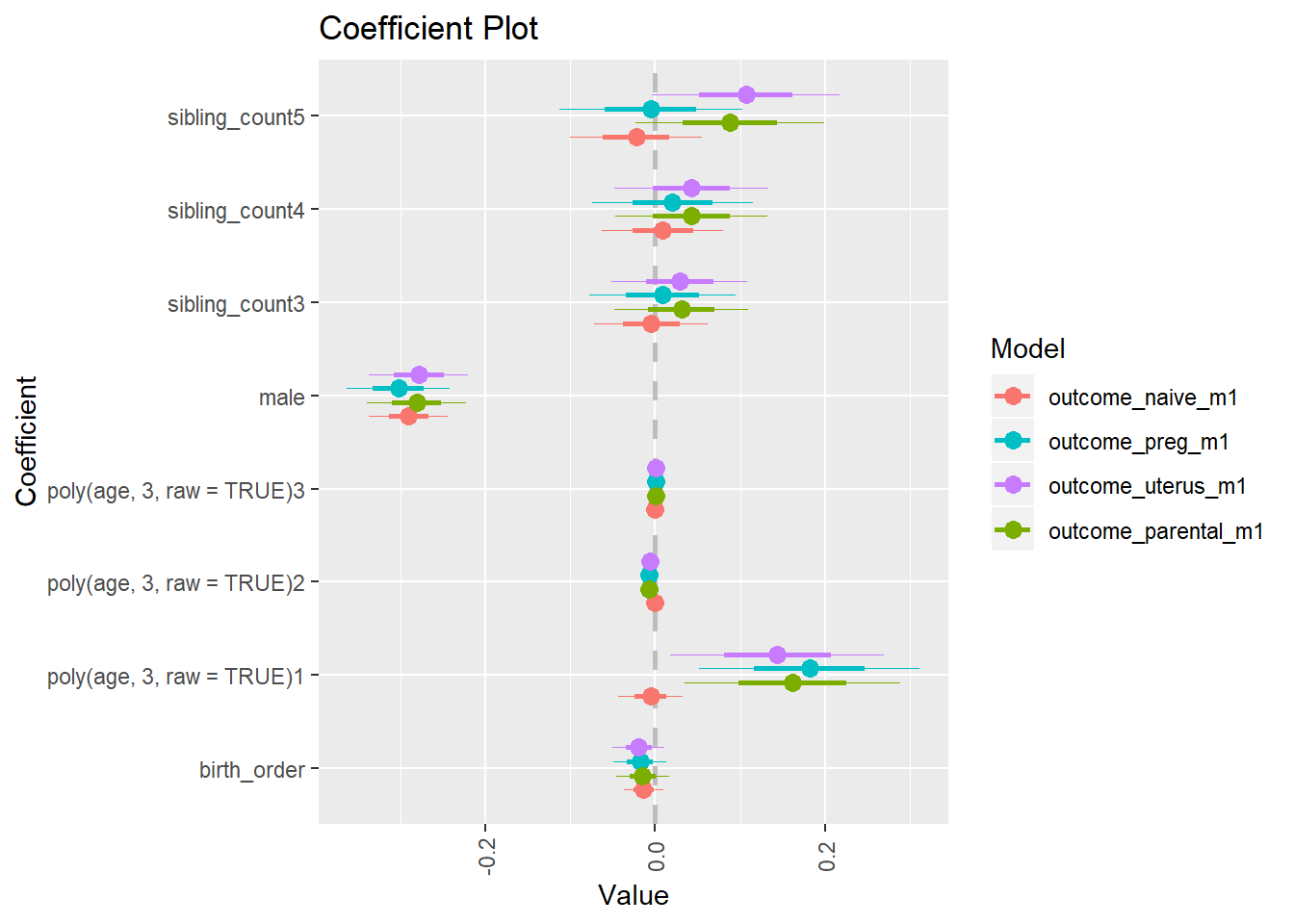
Conscientiousness
birthorder <- birthorder %>% mutate(outcome = big5_con)
model = lmer(outcome ~ birth_order + poly(age, 3, raw = TRUE) + male + sibling_count + (1 | mother_pidlink),
data = birthorder)
compare_birthorder_specs(model)Naive birth order
outcome_naive_m1 <- update(m2_birthorder_linear, data = birthorder %>%
mutate(sibling_count = sibling_count_naive_factor,
birth_order_nonlinear = birthorder_naive_factor,
birth_order = birthorder_naive,
count_birth_order = count_birthorder_naive) %>%
filter(sibling_count != "1"))
compare_models_markdown(outcome_naive_m1)Basic Model
Model Summary
m1_covariates_only <- update(m2_birthorder_linear, formula = . ~ . - birth_order)
tidy(m1_covariates_only, conf.int = T, conf.level = 0.995)| effect | group | term | estimate | std.error | statistic | df | p.value | conf.low | conf.high |
|---|---|---|---|---|---|---|---|---|---|
| fixed | NA | (Intercept) | -1.47 | 0.1995 | -7.367 | 6662 | 1.949e-13 | -2.029 | -0.9097 |
| fixed | NA | poly(age, 3, raw = TRUE)1 | 0.08787 | 0.01915 | 4.588 | 6467 | 0.000004563 | 0.03411 | 0.1416 |
| fixed | NA | poly(age, 3, raw = TRUE)2 | -0.001427 | 0.0005591 | -2.553 | 6253 | 0.01071 | -0.002997 | 0.0001421 |
| fixed | NA | poly(age, 3, raw = TRUE)3 | 0.000007095 | 0.000005071 | 1.399 | 6090 | 0.1618 | -0.000007139 | 0.00002133 |
| fixed | NA | male | 0.03101 | 0.02331 | 1.33 | 7074 | 0.1834 | -0.03442 | 0.09645 |
| fixed | NA | sibling_count3 | -0.01205 | 0.03315 | -0.3634 | 4930 | 0.7163 | -0.1051 | 0.08101 |
| fixed | NA | sibling_count4 | -0.0115 | 0.03412 | -0.337 | 4334 | 0.7361 | -0.1073 | 0.08428 |
| fixed | NA | sibling_count5 | -0.003066 | 0.03542 | -0.08656 | 3711 | 0.931 | -0.1025 | 0.09637 |
| ran_pars | mother_pidlink | sd__(Intercept) | 0.2647 | NA | NA | NA | NA | NA | NA |
| ran_pars | Residual | sd__Observation | 0.9501 | NA | NA | NA | NA | NA | NA |
Coefficient Plot
plot(allEffects(m1_covariates_only, confidence.level = 0.995))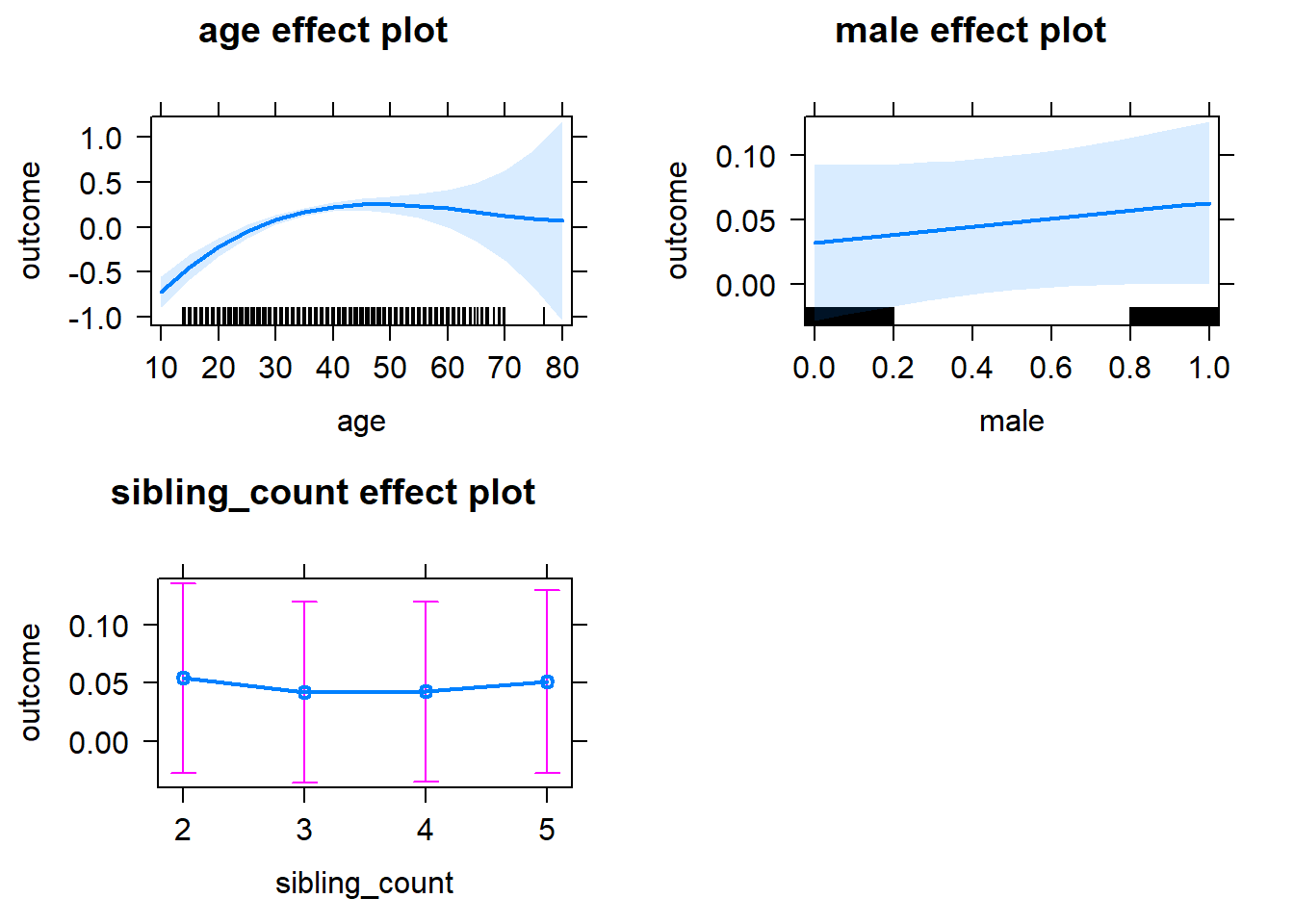
Add Birth Order Linear
Model Summary
tidy(m2_birthorder_linear, conf.int = T, conf.level = 0.995)| effect | group | term | estimate | std.error | statistic | df | p.value | conf.low | conf.high |
|---|---|---|---|---|---|---|---|---|---|
| fixed | NA | (Intercept) | -1.458 | 0.1995 | -7.312 | 6654 | 2.943e-13 | -2.018 | -0.8985 |
| fixed | NA | birth_order | -0.03218 | 0.01167 | -2.758 | 6109 | 0.005835 | -0.06494 | 0.0005733 |
| fixed | NA | poly(age, 3, raw = TRUE)1 | 0.09109 | 0.01918 | 4.748 | 6500 | 0.000002095 | 0.03724 | 0.1449 |
| fixed | NA | poly(age, 3, raw = TRUE)2 | -0.001509 | 0.0005598 | -2.696 | 6273 | 0.007042 | -0.00308 | 0.00006229 |
| fixed | NA | poly(age, 3, raw = TRUE)3 | 0.000007626 | 0.000005074 | 1.503 | 6103 | 0.1329 | -0.000006616 | 0.00002187 |
| fixed | NA | male | 0.03193 | 0.0233 | 1.37 | 7070 | 0.1706 | -0.03348 | 0.09734 |
| fixed | NA | sibling_count3 | -0.0005436 | 0.03342 | -0.01627 | 5064 | 0.987 | -0.09434 | 0.09326 |
| fixed | NA | sibling_count4 | 0.01531 | 0.03548 | 0.4315 | 4906 | 0.6661 | -0.08429 | 0.1149 |
| fixed | NA | sibling_count5 | 0.04002 | 0.03873 | 1.033 | 4853 | 0.3015 | -0.0687 | 0.1487 |
| ran_pars | mother_pidlink | sd__(Intercept) | 0.2673 | NA | NA | NA | NA | NA | NA |
| ran_pars | Residual | sd__Observation | 0.949 | NA | NA | NA | NA | NA | NA |
Coefficient Plot
plot_birthorder2(m2_birthorder_linear, separate = FALSE)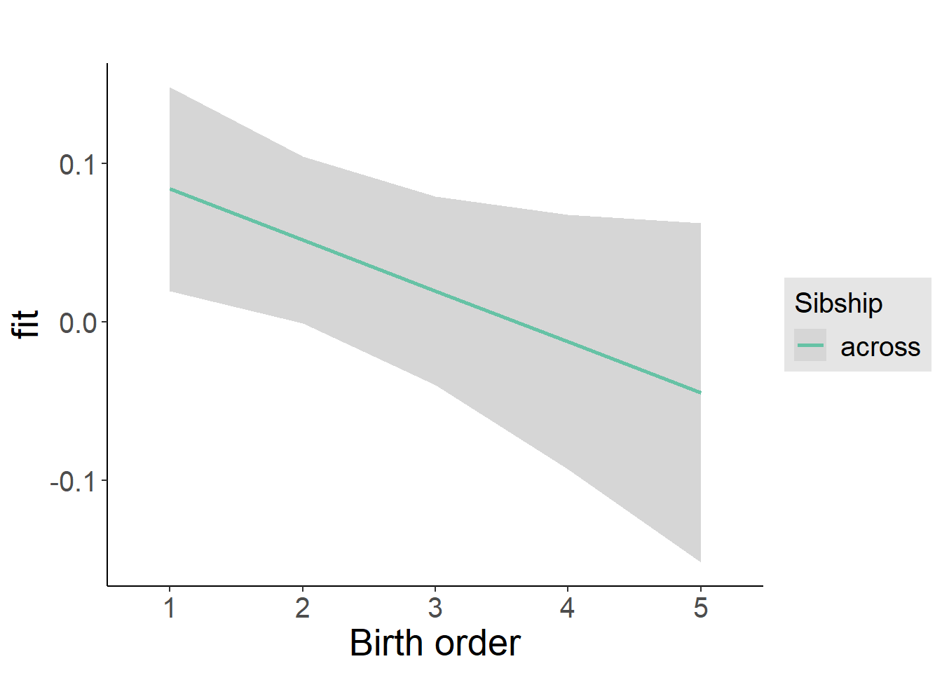
Add Birth Order Factor
Model Summary
m3_birthorder_nonlinear = update(m1_covariates_only, formula = . ~ . + birth_order_nonlinear)
tidy(m3_birthorder_nonlinear, conf.int = T, conf.level = 0.995)| effect | group | term | estimate | std.error | statistic | df | p.value | conf.low | conf.high |
|---|---|---|---|---|---|---|---|---|---|
| fixed | NA | (Intercept) | -1.471 | 0.2 | -7.355 | 6680 | 2.145e-13 | -2.033 | -0.9096 |
| fixed | NA | poly(age, 3, raw = TRUE)1 | 0.09023 | 0.01919 | 4.701 | 6486 | 0.000002641 | 0.03635 | 0.1441 |
| fixed | NA | poly(age, 3, raw = TRUE)2 | -0.001482 | 0.0005602 | -2.645 | 6249 | 0.008185 | -0.003054 | 0.00009066 |
| fixed | NA | poly(age, 3, raw = TRUE)3 | 0.000007368 | 0.000005079 | 1.451 | 6067 | 0.1469 | -0.00000689 | 0.00002163 |
| fixed | NA | male | 0.03195 | 0.0233 | 1.371 | 7067 | 0.1704 | -0.03346 | 0.09736 |
| fixed | NA | sibling_count3 | -0.005349 | 0.03396 | -0.1575 | 5290 | 0.8749 | -0.1007 | 0.08998 |
| fixed | NA | sibling_count4 | 0.005625 | 0.03609 | 0.1559 | 5162 | 0.8762 | -0.09568 | 0.1069 |
| fixed | NA | sibling_count5 | 0.03633 | 0.03912 | 0.9286 | 5039 | 0.3531 | -0.07348 | 0.1461 |
| fixed | NA | birth_order_nonlinear2 | -0.06284 | 0.02774 | -2.266 | 5961 | 0.0235 | -0.1407 | 0.01501 |
| fixed | NA | birth_order_nonlinear3 | -0.05089 | 0.0356 | -1.43 | 5936 | 0.1529 | -0.1508 | 0.04903 |
| fixed | NA | birth_order_nonlinear4 | -0.07589 | 0.04649 | -1.632 | 5955 | 0.1026 | -0.2064 | 0.05461 |
| fixed | NA | birth_order_nonlinear5 | -0.1737 | 0.06767 | -2.567 | 5842 | 0.01028 | -0.3637 | 0.01623 |
| ran_pars | mother_pidlink | sd__(Intercept) | 0.2675 | NA | NA | NA | NA | NA | NA |
| ran_pars | Residual | sd__Observation | 0.9489 | NA | NA | NA | NA | NA | NA |
Coefficient Plot
plot_birthorder(m3_birthorder_nonlinear, separate = FALSE)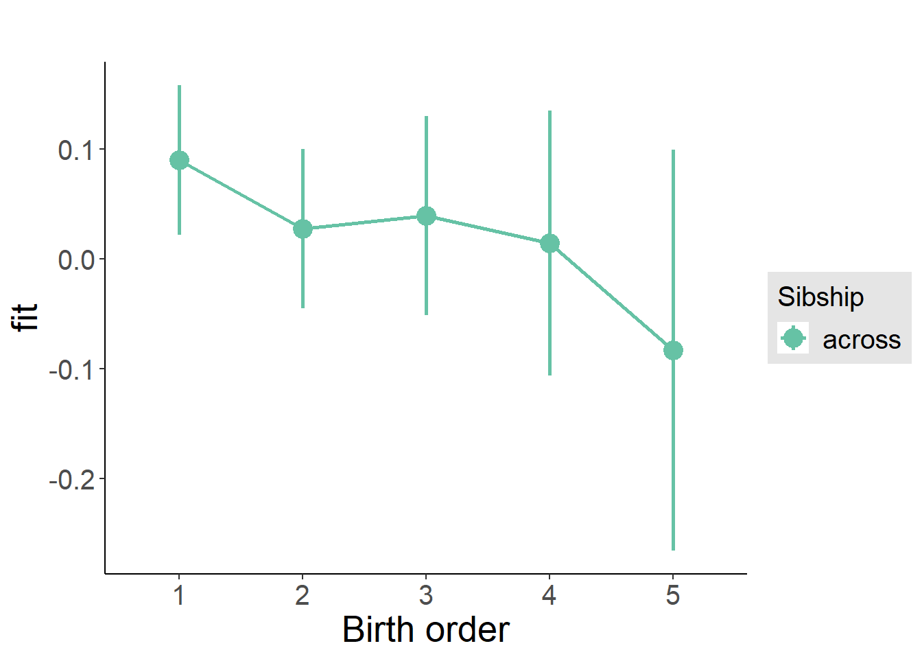
Add Interaction
Model Summary
m4_interaction = update(m3_birthorder_nonlinear, formula = . ~ . - birth_order_nonlinear - sibling_count + count_birth_order)
tidy(m4_interaction, conf.int = T, conf.level = 0.995)| effect | group | term | estimate | std.error | statistic | df | p.value | conf.low | conf.high |
|---|---|---|---|---|---|---|---|---|---|
| fixed | NA | (Intercept) | -1.448 | 0.2004 | -7.223 | 6686 | 5.669e-13 | -2.01 | -0.885 |
| fixed | NA | poly(age, 3, raw = TRUE)1 | 0.09029 | 0.01919 | 4.704 | 6484 | 0.000002602 | 0.03641 | 0.1442 |
| fixed | NA | poly(age, 3, raw = TRUE)2 | -0.001478 | 0.0005602 | -2.638 | 6244 | 0.008357 | -0.00305 | 0.00009461 |
| fixed | NA | poly(age, 3, raw = TRUE)3 | 0.000007284 | 0.00000508 | 1.434 | 6059 | 0.1516 | -0.000006974 | 0.00002154 |
| fixed | NA | male | 0.03158 | 0.02331 | 1.355 | 7060 | 0.1755 | -0.03385 | 0.09701 |
| fixed | NA | count_birth_order2/2 | -0.1321 | 0.04734 | -2.791 | 5893 | 0.005273 | -0.265 | 0.0007633 |
| fixed | NA | count_birth_order1/3 | -0.06049 | 0.04449 | -1.36 | 7116 | 0.174 | -0.1854 | 0.0644 |
| fixed | NA | count_birth_order2/3 | -0.05489 | 0.04977 | -1.103 | 7126 | 0.27 | -0.1946 | 0.0848 |
| fixed | NA | count_birth_order3/3 | -0.07674 | 0.05581 | -1.375 | 7129 | 0.1692 | -0.2334 | 0.07992 |
| fixed | NA | count_birth_order1/4 | -0.03788 | 0.05084 | -0.7452 | 7127 | 0.4562 | -0.1806 | 0.1048 |
| fixed | NA | count_birth_order2/4 | -0.08253 | 0.05347 | -1.543 | 7128 | 0.1228 | -0.2326 | 0.06757 |
| fixed | NA | count_birth_order3/4 | -0.03697 | 0.05813 | -0.6359 | 7128 | 0.5249 | -0.2001 | 0.1262 |
| fixed | NA | count_birth_order4/4 | -0.1067 | 0.0616 | -1.732 | 7125 | 0.08339 | -0.2796 | 0.06625 |
| fixed | NA | count_birth_order1/5 | 0.02716 | 0.05771 | 0.4706 | 7129 | 0.638 | -0.1348 | 0.1892 |
| fixed | NA | count_birth_order2/5 | -0.03752 | 0.06073 | -0.6178 | 7125 | 0.5367 | -0.208 | 0.133 |
| fixed | NA | count_birth_order3/5 | -0.08859 | 0.06235 | -1.421 | 7123 | 0.1554 | -0.2636 | 0.08644 |
| fixed | NA | count_birth_order4/5 | -0.0528 | 0.06609 | -0.7988 | 7118 | 0.4244 | -0.2383 | 0.1327 |
| fixed | NA | count_birth_order5/5 | -0.1635 | 0.06757 | -2.42 | 7115 | 0.01556 | -0.3532 | 0.02618 |
| ran_pars | mother_pidlink | sd__(Intercept) | 0.2666 | NA | NA | NA | NA | NA | NA |
| ran_pars | Residual | sd__Observation | 0.9492 | NA | NA | NA | NA | NA | NA |
Coefficient Plot
plot_birthorder(m4_interaction)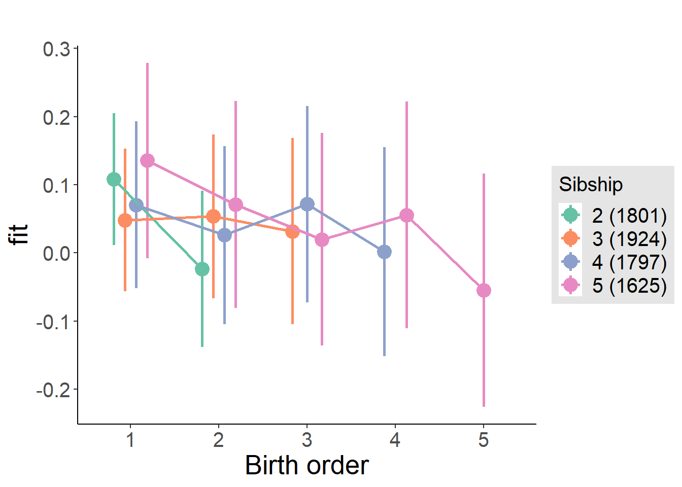
Model Comparison
###### Model 1 - Model 2
anova(m1_covariates_only, m2_birthorder_linear, m3_birthorder_nonlinear, m4_interaction)## refitting model(s) with ML (instead of REML)| Df | AIC | BIC | logLik | deviance | Chisq | Chi Df | Pr(>Chisq) |
|---|---|---|---|---|---|---|---|
| 10 | 20080 | 20149 | -10030 | 20060 | NA | NA | NA |
| 11 | 20075 | 20150 | -10026 | 20053 | 7.597 | 1 | 0.005845 |
| 14 | 20078 | 20174 | -10025 | 20050 | 2.76 | 3 | 0.4301 |
| 20 | 20084 | 20222 | -10022 | 20044 | 5.739 | 6 | 0.4531 |
Maternal birth order
outcome_uterus_m1 <- update(m2_birthorder_linear, data = birthorder %>%
mutate(sibling_count = sibling_count_uterus_alive_factor,
birth_order_nonlinear = birthorder_uterus_alive_factor,
birth_order = birthorder_uterus_alive,
count_birth_order = count_birthorder_uterus_alive) %>%
filter(sibling_count != "1"))
compare_models_markdown(outcome_uterus_m1)Basic Model
Model Summary
m1_covariates_only <- update(m2_birthorder_linear, formula = . ~ . - birth_order)
tidy(m1_covariates_only, conf.int = T, conf.level = 0.995)| effect | group | term | estimate | std.error | statistic | df | p.value | conf.low | conf.high |
|---|---|---|---|---|---|---|---|---|---|
| fixed | NA | (Intercept) | -1.099 | 0.5525 | -1.989 | 4498 | 0.04672 | -2.65 | 0.4518 |
| fixed | NA | poly(age, 3, raw = TRUE)1 | 0.04192 | 0.06446 | 0.6504 | 4494 | 0.5155 | -0.139 | 0.2229 |
| fixed | NA | poly(age, 3, raw = TRUE)2 | 0.0002302 | 0.002375 | 0.09693 | 4487 | 0.9228 | -0.006435 | 0.006896 |
| fixed | NA | poly(age, 3, raw = TRUE)3 | -0.00000977 | 0.00002781 | -0.3513 | 4481 | 0.7254 | -0.00008784 | 0.0000683 |
| fixed | NA | male | 0.04417 | 0.02981 | 1.482 | 4477 | 0.1385 | -0.0395 | 0.1279 |
| fixed | NA | sibling_count3 | -0.02662 | 0.04006 | -0.6644 | 3248 | 0.5065 | -0.1391 | 0.08583 |
| fixed | NA | sibling_count4 | -0.04555 | 0.04309 | -1.057 | 2744 | 0.2905 | -0.1665 | 0.07539 |
| fixed | NA | sibling_count5 | -0.0141 | 0.04901 | -0.2876 | 2343 | 0.7736 | -0.1517 | 0.1235 |
| ran_pars | mother_pidlink | sd__(Intercept) | 0.2378 | NA | NA | NA | NA | NA | NA |
| ran_pars | Residual | sd__Observation | 0.972 | NA | NA | NA | NA | NA | NA |
Coefficient Plot
plot(allEffects(m1_covariates_only, confidence.level = 0.995))
Add Birth Order Linear
Model Summary
tidy(m2_birthorder_linear, conf.int = T, conf.level = 0.995)| effect | group | term | estimate | std.error | statistic | df | p.value | conf.low | conf.high |
|---|---|---|---|---|---|---|---|---|---|
| fixed | NA | (Intercept) | -1.033 | 0.5528 | -1.868 | 4497 | 0.0618 | -2.584 | 0.519 |
| fixed | NA | birth_order | -0.03961 | 0.01569 | -2.524 | 4208 | 0.01165 | -0.08366 | 0.004447 |
| fixed | NA | poly(age, 3, raw = TRUE)1 | 0.03953 | 0.06443 | 0.6135 | 4493 | 0.5396 | -0.1413 | 0.2204 |
| fixed | NA | poly(age, 3, raw = TRUE)2 | 0.0003663 | 0.002374 | 0.1543 | 4488 | 0.8774 | -0.006297 | 0.00703 |
| fixed | NA | poly(age, 3, raw = TRUE)3 | -0.00001217 | 0.00002781 | -0.4376 | 4481 | 0.6617 | -0.00009025 | 0.0000659 |
| fixed | NA | male | 0.0454 | 0.0298 | 1.524 | 4475 | 0.1276 | -0.03823 | 0.129 |
| fixed | NA | sibling_count3 | -0.008487 | 0.04069 | -0.2086 | 3316 | 0.8348 | -0.1227 | 0.1057 |
| fixed | NA | sibling_count4 | -0.004046 | 0.04612 | -0.08773 | 2999 | 0.9301 | -0.1335 | 0.1254 |
| fixed | NA | sibling_count5 | 0.05526 | 0.05622 | 0.9828 | 2902 | 0.3258 | -0.1026 | 0.2131 |
| ran_pars | mother_pidlink | sd__(Intercept) | 0.2421 | NA | NA | NA | NA | NA | NA |
| ran_pars | Residual | sd__Observation | 0.9704 | NA | NA | NA | NA | NA | NA |
Coefficient Plot
plot_birthorder2(m2_birthorder_linear, separate = FALSE)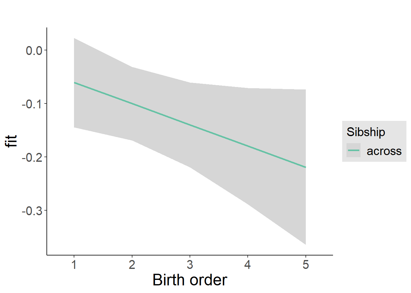
Add Birth Order Factor
Model Summary
m3_birthorder_nonlinear = update(m1_covariates_only, formula = . ~ . + birth_order_nonlinear)
tidy(m3_birthorder_nonlinear, conf.int = T, conf.level = 0.995)| effect | group | term | estimate | std.error | statistic | df | p.value | conf.low | conf.high |
|---|---|---|---|---|---|---|---|---|---|
| fixed | NA | (Intercept) | -1.077 | 0.5532 | -1.947 | 4492 | 0.05163 | -2.63 | 0.4759 |
| fixed | NA | poly(age, 3, raw = TRUE)1 | 0.0406 | 0.06449 | 0.6296 | 4488 | 0.529 | -0.1404 | 0.2216 |
| fixed | NA | poly(age, 3, raw = TRUE)2 | 0.0003283 | 0.002376 | 0.1382 | 4481 | 0.8901 | -0.006341 | 0.006998 |
| fixed | NA | poly(age, 3, raw = TRUE)3 | -0.00001179 | 0.00002784 | -0.4236 | 4475 | 0.6719 | -0.00008993 | 0.00006635 |
| fixed | NA | male | 0.04547 | 0.02981 | 1.525 | 4472 | 0.1272 | -0.0382 | 0.1291 |
| fixed | NA | sibling_count3 | -0.0181 | 0.04137 | -0.4374 | 3448 | 0.6618 | -0.1342 | 0.09802 |
| fixed | NA | sibling_count4 | -0.01065 | 0.04685 | -0.2274 | 3108 | 0.8201 | -0.1421 | 0.1208 |
| fixed | NA | sibling_count5 | 0.05809 | 0.05721 | 1.015 | 2992 | 0.31 | -0.1025 | 0.2187 |
| fixed | NA | birth_order_nonlinear2 | -0.05233 | 0.03578 | -1.462 | 3633 | 0.1437 | -0.1528 | 0.04811 |
| fixed | NA | birth_order_nonlinear3 | -0.03777 | 0.04553 | -0.8295 | 3886 | 0.4069 | -0.1656 | 0.09003 |
| fixed | NA | birth_order_nonlinear4 | -0.1355 | 0.06104 | -2.22 | 4092 | 0.02645 | -0.3069 | 0.03581 |
| fixed | NA | birth_order_nonlinear5 | -0.2042 | 0.09514 | -2.147 | 3979 | 0.03189 | -0.4713 | 0.06284 |
| ran_pars | mother_pidlink | sd__(Intercept) | 0.2405 | NA | NA | NA | NA | NA | NA |
| ran_pars | Residual | sd__Observation | 0.9709 | NA | NA | NA | NA | NA | NA |
Coefficient Plot
plot_birthorder(m3_birthorder_nonlinear, separate = FALSE)
Add Interaction
Model Summary
m4_interaction = update(m3_birthorder_nonlinear, formula = . ~ . - birth_order_nonlinear - sibling_count + count_birth_order)
tidy(m4_interaction, conf.int = T, conf.level = 0.995)| effect | group | term | estimate | std.error | statistic | df | p.value | conf.low | conf.high |
|---|---|---|---|---|---|---|---|---|---|
| fixed | NA | (Intercept) | -1.062 | 0.5533 | -1.919 | 4486 | 0.05501 | -2.615 | 0.4912 |
| fixed | NA | poly(age, 3, raw = TRUE)1 | 0.04168 | 0.0645 | 0.6462 | 4483 | 0.5182 | -0.1394 | 0.2227 |
| fixed | NA | poly(age, 3, raw = TRUE)2 | 0.0002473 | 0.002377 | 0.104 | 4476 | 0.9171 | -0.006424 | 0.006918 |
| fixed | NA | poly(age, 3, raw = TRUE)3 | -0.00001032 | 0.00002785 | -0.3706 | 4470 | 0.7109 | -0.00008849 | 0.00006785 |
| fixed | NA | male | 0.04612 | 0.02982 | 1.547 | 4466 | 0.122 | -0.03758 | 0.1298 |
| fixed | NA | count_birth_order2/2 | -0.1015 | 0.06133 | -1.654 | 3783 | 0.09812 | -0.2736 | 0.07069 |
| fixed | NA | count_birth_order1/3 | -0.005411 | 0.05361 | -0.1009 | 4487 | 0.9196 | -0.1559 | 0.1451 |
| fixed | NA | count_birth_order2/3 | -0.1003 | 0.0586 | -1.712 | 4490 | 0.08705 | -0.2648 | 0.06419 |
| fixed | NA | count_birth_order3/3 | -0.1107 | 0.06554 | -1.69 | 4487 | 0.09116 | -0.2947 | 0.07323 |
| fixed | NA | count_birth_order1/4 | -0.06003 | 0.06578 | -0.9126 | 4487 | 0.3615 | -0.2447 | 0.1246 |
| fixed | NA | count_birth_order2/4 | -0.06124 | 0.06801 | -0.9005 | 4490 | 0.3679 | -0.2521 | 0.1297 |
| fixed | NA | count_birth_order3/4 | -0.02798 | 0.07186 | -0.3893 | 4484 | 0.6971 | -0.2297 | 0.1737 |
| fixed | NA | count_birth_order4/4 | -0.1808 | 0.07465 | -2.422 | 4482 | 0.01546 | -0.3904 | 0.02873 |
| fixed | NA | count_birth_order1/5 | -0.09531 | 0.08953 | -1.064 | 4490 | 0.2872 | -0.3466 | 0.156 |
| fixed | NA | count_birth_order2/5 | 0.09181 | 0.09565 | 0.9598 | 4484 | 0.3372 | -0.1767 | 0.3603 |
| fixed | NA | count_birth_order3/5 | 0.02478 | 0.08963 | 0.2765 | 4479 | 0.7822 | -0.2268 | 0.2764 |
| fixed | NA | count_birth_order4/5 | -0.06633 | 0.08629 | -0.7687 | 4480 | 0.4421 | -0.3085 | 0.1759 |
| fixed | NA | count_birth_order5/5 | -0.1617 | 0.08976 | -1.802 | 4472 | 0.07164 | -0.4137 | 0.09023 |
| ran_pars | mother_pidlink | sd__(Intercept) | 0.239 | NA | NA | NA | NA | NA | NA |
| ran_pars | Residual | sd__Observation | 0.9711 | NA | NA | NA | NA | NA | NA |
Coefficient Plot
plot_birthorder(m4_interaction)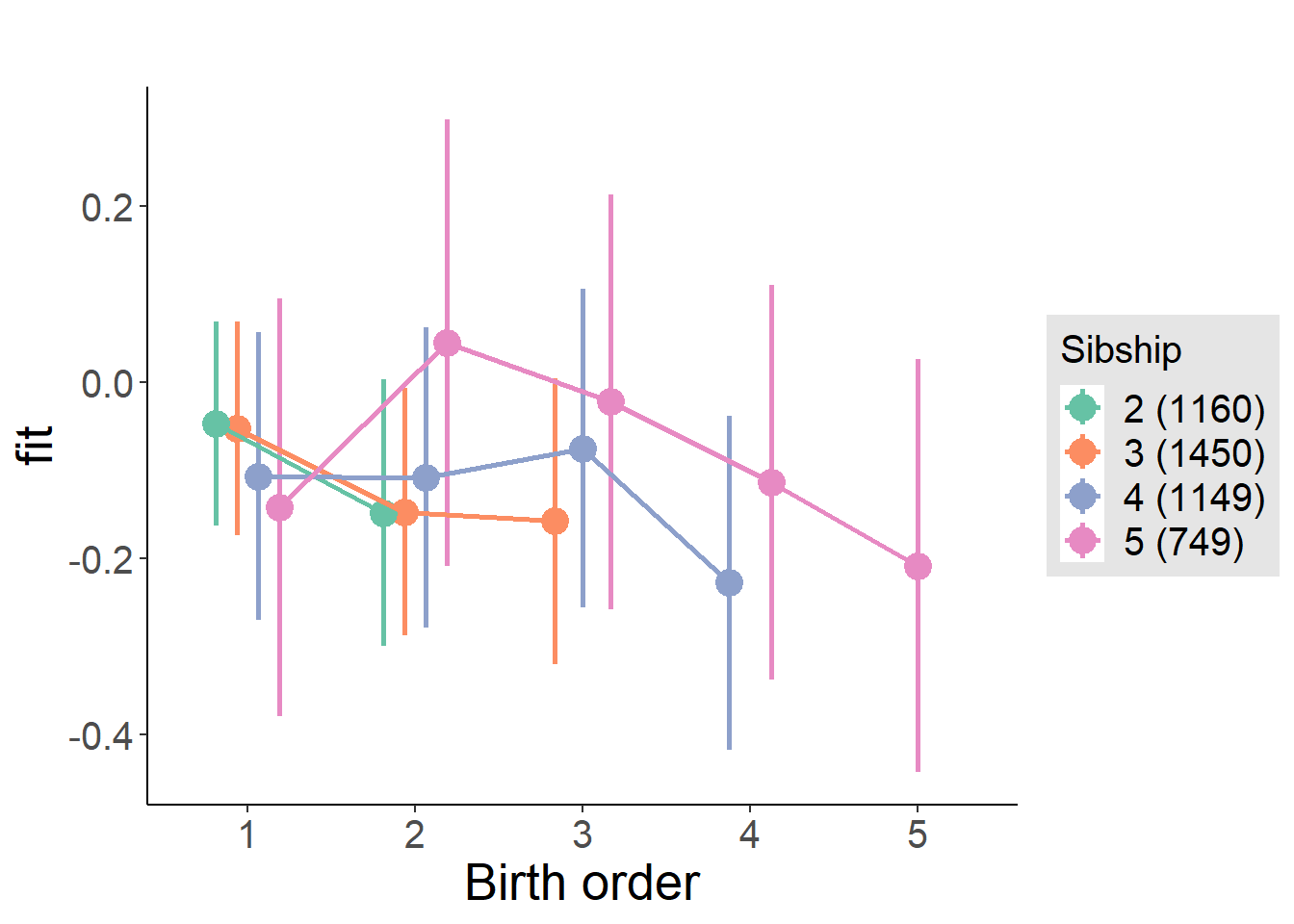
Model Comparison
###### Model 1 - Model 2
anova(m1_covariates_only, m2_birthorder_linear, m3_birthorder_nonlinear, m4_interaction)## refitting model(s) with ML (instead of REML)| Df | AIC | BIC | logLik | deviance | Chisq | Chi Df | Pr(>Chisq) |
|---|---|---|---|---|---|---|---|
| 10 | 12806 | 12870 | -6393 | 12786 | NA | NA | NA |
| 11 | 12801 | 12872 | -6390 | 12779 | 6.362 | 1 | 0.01166 |
| 14 | 12805 | 12895 | -6389 | 12777 | 1.86 | 3 | 0.602 |
| 20 | 12810 | 12939 | -6385 | 12770 | 7.234 | 6 | 0.2998 |
Maternal pregnancy order
outcome_preg_m1 <- update(m2_birthorder_linear, data = birthorder %>%
mutate(sibling_count = sibling_count_uterus_preg_factor,
birth_order_nonlinear = birthorder_uterus_preg_factor,
birth_order = birthorder_uterus_preg,
count_birth_order = count_birthorder_uterus_preg
) %>%
filter(sibling_count != "1"))
compare_models_markdown(outcome_preg_m1)Basic Model
Model Summary
m1_covariates_only <- update(m2_birthorder_linear, formula = . ~ . - birth_order)
tidy(m1_covariates_only, conf.int = T, conf.level = 0.995)| effect | group | term | estimate | std.error | statistic | df | p.value | conf.low | conf.high |
|---|---|---|---|---|---|---|---|---|---|
| fixed | NA | (Intercept) | -1.313 | 0.5685 | -2.309 | 4175 | 0.02097 | -2.909 | 0.283 |
| fixed | NA | poly(age, 3, raw = TRUE)1 | 0.07063 | 0.06638 | 1.064 | 4171 | 0.2874 | -0.1157 | 0.257 |
| fixed | NA | poly(age, 3, raw = TRUE)2 | -0.0008233 | 0.002446 | -0.3366 | 4164 | 0.7365 | -0.00769 | 0.006043 |
| fixed | NA | poly(age, 3, raw = TRUE)3 | 0.000002617 | 0.00002865 | 0.09135 | 4157 | 0.9272 | -0.00007781 | 0.00008305 |
| fixed | NA | male | 0.03828 | 0.03094 | 1.237 | 4158 | 0.216 | -0.04856 | 0.1251 |
| fixed | NA | sibling_count3 | -0.07058 | 0.04322 | -1.633 | 3127 | 0.1026 | -0.1919 | 0.05075 |
| fixed | NA | sibling_count4 | -0.06824 | 0.04555 | -1.498 | 2774 | 0.1342 | -0.1961 | 0.05962 |
| fixed | NA | sibling_count5 | -0.06113 | 0.0486 | -1.258 | 2387 | 0.2086 | -0.1975 | 0.07528 |
| ran_pars | mother_pidlink | sd__(Intercept) | 0.2159 | NA | NA | NA | NA | NA | NA |
| ran_pars | Residual | sd__Observation | 0.976 | NA | NA | NA | NA | NA | NA |
Coefficient Plot
plot(allEffects(m1_covariates_only, confidence.level = 0.995))
Add Birth Order Linear
Model Summary
tidy(m2_birthorder_linear, conf.int = T, conf.level = 0.995)| effect | group | term | estimate | std.error | statistic | df | p.value | conf.low | conf.high |
|---|---|---|---|---|---|---|---|---|---|
| fixed | NA | (Intercept) | -1.254 | 0.5688 | -2.204 | 4174 | 0.02755 | -2.851 | 0.3428 |
| fixed | NA | birth_order | -0.03564 | 0.01572 | -2.268 | 3996 | 0.0234 | -0.07977 | 0.008477 |
| fixed | NA | poly(age, 3, raw = TRUE)1 | 0.06867 | 0.06635 | 1.035 | 4170 | 0.3008 | -0.1176 | 0.2549 |
| fixed | NA | poly(age, 3, raw = TRUE)2 | -0.0007097 | 0.002446 | -0.2902 | 4164 | 0.7717 | -0.007574 | 0.006155 |
| fixed | NA | poly(age, 3, raw = TRUE)3 | 0.0000005678 | 0.00002865 | 0.01981 | 4158 | 0.9842 | -0.00007987 | 0.000081 |
| fixed | NA | male | 0.03898 | 0.03092 | 1.261 | 4156 | 0.2075 | -0.04781 | 0.1258 |
| fixed | NA | sibling_count3 | -0.05432 | 0.04381 | -1.24 | 3174 | 0.215 | -0.1773 | 0.06864 |
| fixed | NA | sibling_count4 | -0.03216 | 0.04825 | -0.6665 | 2959 | 0.5051 | -0.1676 | 0.1033 |
| fixed | NA | sibling_count5 | -0.003572 | 0.05485 | -0.06511 | 2822 | 0.9481 | -0.1575 | 0.1504 |
| ran_pars | mother_pidlink | sd__(Intercept) | 0.2197 | NA | NA | NA | NA | NA | NA |
| ran_pars | Residual | sd__Observation | 0.9746 | NA | NA | NA | NA | NA | NA |
Coefficient Plot
plot_birthorder2(m2_birthorder_linear, separate = FALSE)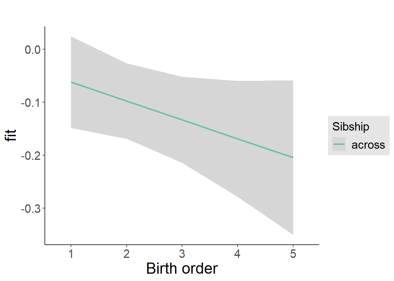
Add Birth Order Factor
Model Summary
m3_birthorder_nonlinear = update(m1_covariates_only, formula = . ~ . + birth_order_nonlinear)
tidy(m3_birthorder_nonlinear, conf.int = T, conf.level = 0.995)| effect | group | term | estimate | std.error | statistic | df | p.value | conf.low | conf.high |
|---|---|---|---|---|---|---|---|---|---|
| fixed | NA | (Intercept) | -1.263 | 0.5692 | -2.219 | 4169 | 0.02655 | -2.861 | 0.3347 |
| fixed | NA | poly(age, 3, raw = TRUE)1 | 0.0667 | 0.0664 | 1.004 | 4164 | 0.3152 | -0.1197 | 0.2531 |
| fixed | NA | poly(age, 3, raw = TRUE)2 | -0.0006384 | 0.002447 | -0.2609 | 4158 | 0.7942 | -0.007508 | 0.006231 |
| fixed | NA | poly(age, 3, raw = TRUE)3 | -0.0000002049 | 0.00002867 | -0.007144 | 4152 | 0.9943 | -0.00008069 | 0.00008028 |
| fixed | NA | male | 0.03836 | 0.03093 | 1.24 | 4154 | 0.215 | -0.04847 | 0.1252 |
| fixed | NA | sibling_count3 | -0.05133 | 0.04449 | -1.154 | 3286 | 0.2487 | -0.1762 | 0.07355 |
| fixed | NA | sibling_count4 | -0.03892 | 0.04896 | -0.7949 | 3060 | 0.4267 | -0.1764 | 0.09852 |
| fixed | NA | sibling_count5 | -0.006557 | 0.05543 | -0.1183 | 2870 | 0.9058 | -0.1622 | 0.149 |
| fixed | NA | birth_order_nonlinear2 | -0.065 | 0.03728 | -1.744 | 3457 | 0.08128 | -0.1696 | 0.03963 |
| fixed | NA | birth_order_nonlinear3 | -0.08652 | 0.04703 | -1.84 | 3710 | 0.06589 | -0.2185 | 0.04549 |
| fixed | NA | birth_order_nonlinear4 | -0.06627 | 0.06214 | -1.066 | 3871 | 0.2863 | -0.2407 | 0.1082 |
| fixed | NA | birth_order_nonlinear5 | -0.1763 | 0.09115 | -1.934 | 3795 | 0.05321 | -0.4321 | 0.07959 |
| ran_pars | mother_pidlink | sd__(Intercept) | 0.2164 | NA | NA | NA | NA | NA | NA |
| ran_pars | Residual | sd__Observation | 0.9755 | NA | NA | NA | NA | NA | NA |
Coefficient Plot
plot_birthorder(m3_birthorder_nonlinear, separate = FALSE)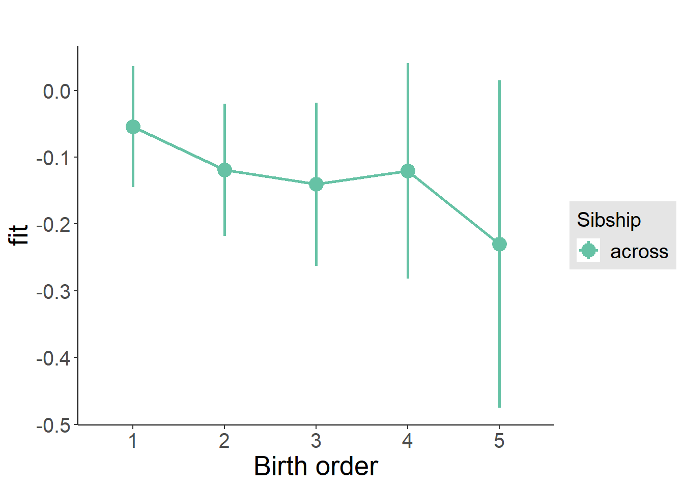
Add Interaction
Model Summary
m4_interaction = update(m3_birthorder_nonlinear, formula = . ~ . - birth_order_nonlinear - sibling_count + count_birth_order)
tidy(m4_interaction, conf.int = T, conf.level = 0.995)| effect | group | term | estimate | std.error | statistic | df | p.value | conf.low | conf.high |
|---|---|---|---|---|---|---|---|---|---|
| fixed | NA | (Intercept) | -1.266 | 0.5697 | -2.222 | 4163 | 0.02637 | -2.865 | 0.3336 |
| fixed | NA | poly(age, 3, raw = TRUE)1 | 0.0677 | 0.06646 | 1.019 | 4159 | 0.3084 | -0.1188 | 0.2542 |
| fixed | NA | poly(age, 3, raw = TRUE)2 | -0.00069 | 0.002449 | -0.2817 | 4153 | 0.7782 | -0.007566 | 0.006186 |
| fixed | NA | poly(age, 3, raw = TRUE)3 | 0.0000005663 | 0.0000287 | 0.01973 | 4146 | 0.9843 | -0.00008 | 0.00008114 |
| fixed | NA | male | 0.03937 | 0.03096 | 1.271 | 4147 | 0.2036 | -0.04754 | 0.1263 |
| fixed | NA | count_birth_order2/2 | -0.07457 | 0.06716 | -1.11 | 3572 | 0.2669 | -0.2631 | 0.114 |
| fixed | NA | count_birth_order1/3 | -0.04803 | 0.05804 | -0.8275 | 4165 | 0.408 | -0.2109 | 0.1149 |
| fixed | NA | count_birth_order2/3 | -0.1054 | 0.06295 | -1.675 | 4167 | 0.094 | -0.2821 | 0.07126 |
| fixed | NA | count_birth_order3/3 | -0.1743 | 0.07089 | -2.459 | 4164 | 0.01396 | -0.3733 | 0.02466 |
| fixed | NA | count_birth_order1/4 | -0.045 | 0.06889 | -0.6533 | 4165 | 0.5136 | -0.2384 | 0.1484 |
| fixed | NA | count_birth_order2/4 | -0.09229 | 0.07014 | -1.316 | 4167 | 0.1883 | -0.2892 | 0.1046 |
| fixed | NA | count_birth_order3/4 | -0.09046 | 0.07696 | -1.175 | 4162 | 0.2399 | -0.3065 | 0.1256 |
| fixed | NA | count_birth_order4/4 | -0.1669 | 0.07926 | -2.106 | 4161 | 0.0353 | -0.3894 | 0.0556 |
| fixed | NA | count_birth_order1/5 | -0.03418 | 0.08198 | -0.4169 | 4166 | 0.6768 | -0.2643 | 0.1959 |
| fixed | NA | count_birth_order2/5 | -0.1247 | 0.08789 | -1.419 | 4166 | 0.1559 | -0.3714 | 0.122 |
| fixed | NA | count_birth_order3/5 | -0.09217 | 0.08538 | -1.08 | 4163 | 0.2804 | -0.3318 | 0.1475 |
| fixed | NA | count_birth_order4/5 | 0.001339 | 0.08846 | 0.01514 | 4156 | 0.9879 | -0.247 | 0.2497 |
| fixed | NA | count_birth_order5/5 | -0.1854 | 0.08864 | -2.092 | 4152 | 0.03648 | -0.4343 | 0.06337 |
| ran_pars | mother_pidlink | sd__(Intercept) | 0.2177 | NA | NA | NA | NA | NA | NA |
| ran_pars | Residual | sd__Observation | 0.9756 | NA | NA | NA | NA | NA | NA |
Coefficient Plot
plot_birthorder(m4_interaction)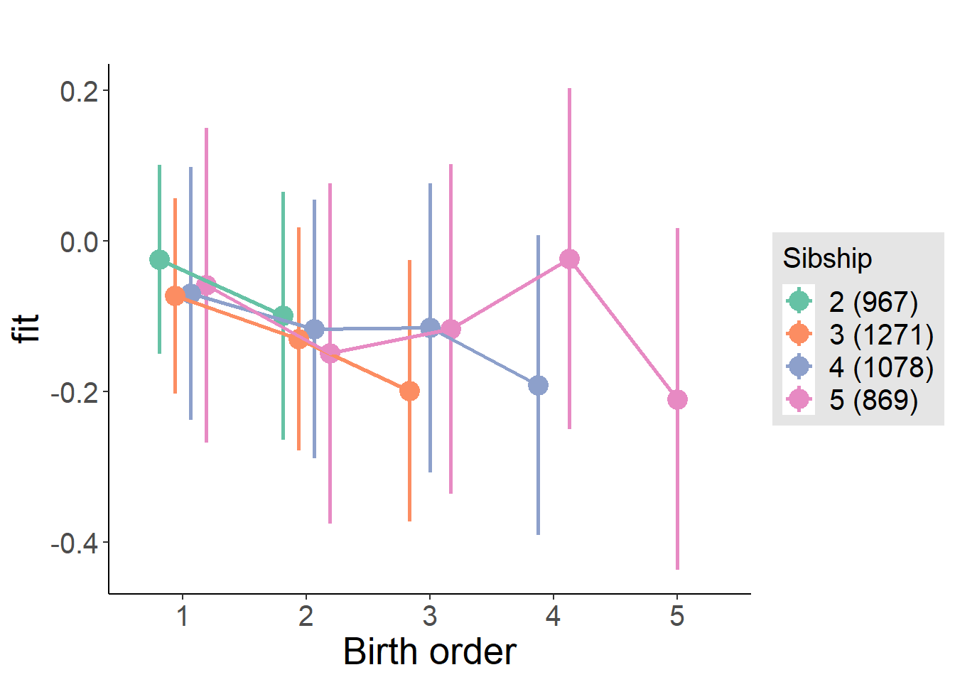
Model Comparison
###### Model 1 - Model 2
anova(m1_covariates_only, m2_birthorder_linear, m3_birthorder_nonlinear, m4_interaction)## refitting model(s) with ML (instead of REML)| Df | AIC | BIC | logLik | deviance | Chisq | Chi Df | Pr(>Chisq) |
|---|---|---|---|---|---|---|---|
| 10 | 11881 | 11945 | -5931 | 11861 | NA | NA | NA |
| 11 | 11878 | 11948 | -5928 | 11856 | 5.14 | 1 | 0.02338 |
| 14 | 11883 | 11971 | -5927 | 11855 | 1.673 | 3 | 0.643 |
| 20 | 11891 | 12018 | -5926 | 11851 | 3.155 | 6 | 0.7892 |
Parental full sibling order
outcome_parental_m1 <- update(m2_birthorder_linear, data = birthorder %>%
mutate(sibling_count = sibling_count_genes_factor,
birth_order_nonlinear = birthorder_genes_factor,
birth_order = birthorder_genes,
count_birth_order = count_birthorder_genes
) %>%
filter(sibling_count != "1"))
compare_models_markdown(outcome_parental_m1)Basic Model
Model Summary
m1_covariates_only <- update(m2_birthorder_linear, formula = . ~ . - birth_order)
tidy(m1_covariates_only, conf.int = T, conf.level = 0.995)| effect | group | term | estimate | std.error | statistic | df | p.value | conf.low | conf.high |
|---|---|---|---|---|---|---|---|---|---|
| fixed | NA | (Intercept) | -0.7774 | 0.5576 | -1.394 | 4483 | 0.1634 | -2.343 | 0.7879 |
| fixed | NA | poly(age, 3, raw = TRUE)1 | 0.006837 | 0.06514 | 0.105 | 4478 | 0.9164 | -0.176 | 0.1897 |
| fixed | NA | poly(age, 3, raw = TRUE)2 | 0.001469 | 0.002403 | 0.611 | 4471 | 0.5412 | -0.005278 | 0.008215 |
| fixed | NA | poly(age, 3, raw = TRUE)3 | -0.00002355 | 0.0000282 | -0.8349 | 4464 | 0.4038 | -0.0001027 | 0.00005562 |
| fixed | NA | male | 0.04058 | 0.02987 | 1.358 | 4464 | 0.1744 | -0.04327 | 0.1244 |
| fixed | NA | sibling_count3 | -0.06404 | 0.03953 | -1.62 | 3211 | 0.1053 | -0.175 | 0.04691 |
| fixed | NA | sibling_count4 | -0.05905 | 0.04275 | -1.381 | 2720 | 0.1673 | -0.1791 | 0.06096 |
| fixed | NA | sibling_count5 | 0.006905 | 0.05013 | 0.1378 | 2213 | 0.8904 | -0.1338 | 0.1476 |
| ran_pars | mother_pidlink | sd__(Intercept) | 0.2339 | NA | NA | NA | NA | NA | NA |
| ran_pars | Residual | sd__Observation | 0.9728 | NA | NA | NA | NA | NA | NA |
Coefficient Plot
plot(allEffects(m1_covariates_only, confidence.level = 0.995))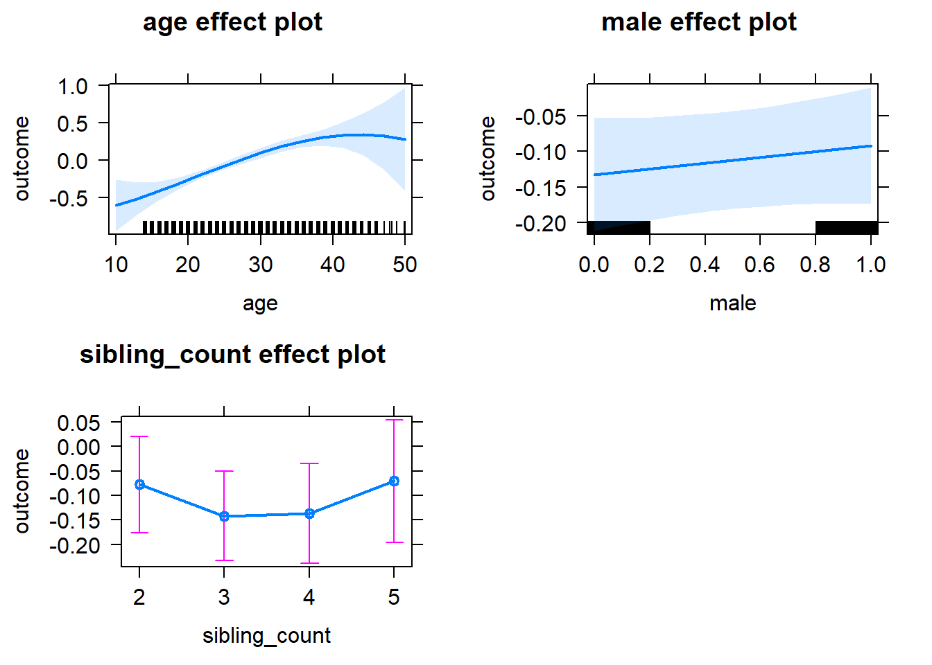
Add Birth Order Linear
Model Summary
tidy(m2_birthorder_linear, conf.int = T, conf.level = 0.995)| effect | group | term | estimate | std.error | statistic | df | p.value | conf.low | conf.high |
|---|---|---|---|---|---|---|---|---|---|
| fixed | NA | (Intercept) | -0.7228 | 0.558 | -1.295 | 4482 | 0.1953 | -2.289 | 0.8437 |
| fixed | NA | birth_order | -0.03318 | 0.01591 | -2.085 | 4177 | 0.0371 | -0.07785 | 0.01148 |
| fixed | NA | poly(age, 3, raw = TRUE)1 | 0.005 | 0.06513 | 0.07678 | 4477 | 0.9388 | -0.1778 | 0.1878 |
| fixed | NA | poly(age, 3, raw = TRUE)2 | 0.001576 | 0.002403 | 0.6557 | 4471 | 0.512 | -0.00517 | 0.008321 |
| fixed | NA | poly(age, 3, raw = TRUE)3 | -0.00002547 | 0.00002821 | -0.903 | 4464 | 0.3666 | -0.0001047 | 0.00005371 |
| fixed | NA | male | 0.04138 | 0.02986 | 1.386 | 4461 | 0.1659 | -0.04244 | 0.1252 |
| fixed | NA | sibling_count3 | -0.04889 | 0.04019 | -1.216 | 3275 | 0.2239 | -0.1617 | 0.06393 |
| fixed | NA | sibling_count4 | -0.02443 | 0.04588 | -0.5325 | 2990 | 0.5944 | -0.1532 | 0.1044 |
| fixed | NA | sibling_count5 | 0.06233 | 0.05678 | 1.098 | 2718 | 0.2724 | -0.09704 | 0.2217 |
| ran_pars | mother_pidlink | sd__(Intercept) | 0.2381 | NA | NA | NA | NA | NA | NA |
| ran_pars | Residual | sd__Observation | 0.9714 | NA | NA | NA | NA | NA | NA |
Coefficient Plot
plot_birthorder2(m2_birthorder_linear, separate = FALSE)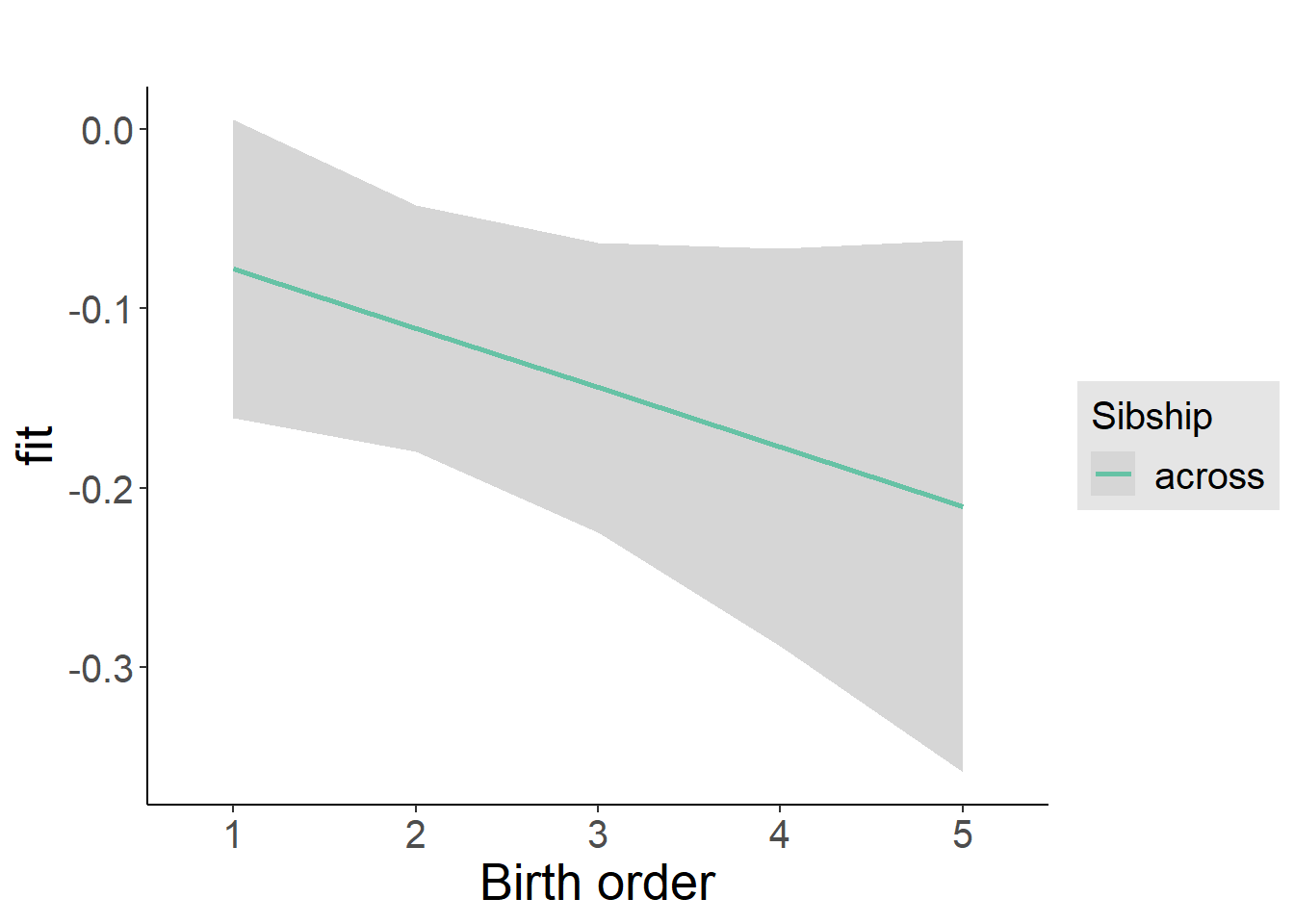
Add Birth Order Factor
Model Summary
m3_birthorder_nonlinear = update(m1_covariates_only, formula = . ~ . + birth_order_nonlinear)
tidy(m3_birthorder_nonlinear, conf.int = T, conf.level = 0.995)| effect | group | term | estimate | std.error | statistic | df | p.value | conf.low | conf.high |
|---|---|---|---|---|---|---|---|---|---|
| fixed | NA | (Intercept) | -0.7631 | 0.5585 | -1.366 | 4476 | 0.1719 | -2.331 | 0.8045 |
| fixed | NA | poly(age, 3, raw = TRUE)1 | 0.006244 | 0.06519 | 0.09579 | 4471 | 0.9237 | -0.1767 | 0.1892 |
| fixed | NA | poly(age, 3, raw = TRUE)2 | 0.001532 | 0.002405 | 0.6371 | 4464 | 0.5241 | -0.005219 | 0.008284 |
| fixed | NA | poly(age, 3, raw = TRUE)3 | -0.00002504 | 0.00002823 | -0.8868 | 4458 | 0.3752 | -0.0001043 | 0.00005421 |
| fixed | NA | male | 0.04204 | 0.02988 | 1.407 | 4458 | 0.1594 | -0.04182 | 0.1259 |
| fixed | NA | sibling_count3 | -0.05789 | 0.04089 | -1.416 | 3415 | 0.1569 | -0.1727 | 0.05689 |
| fixed | NA | sibling_count4 | -0.02594 | 0.04662 | -0.5565 | 3102 | 0.5779 | -0.1568 | 0.1049 |
| fixed | NA | sibling_count5 | 0.06232 | 0.05798 | 1.075 | 2816 | 0.2826 | -0.1004 | 0.2251 |
| fixed | NA | birth_order_nonlinear2 | -0.04423 | 0.0356 | -1.242 | 3616 | 0.2142 | -0.1442 | 0.0557 |
| fixed | NA | birth_order_nonlinear3 | -0.02929 | 0.04542 | -0.6448 | 3843 | 0.5191 | -0.1568 | 0.09821 |
| fixed | NA | birth_order_nonlinear4 | -0.1381 | 0.06241 | -2.212 | 4064 | 0.02701 | -0.3133 | 0.03713 |
| fixed | NA | birth_order_nonlinear5 | -0.1351 | 0.1019 | -1.325 | 4032 | 0.1851 | -0.4211 | 0.151 |
| ran_pars | mother_pidlink | sd__(Intercept) | 0.2369 | NA | NA | NA | NA | NA | NA |
| ran_pars | Residual | sd__Observation | 0.9719 | NA | NA | NA | NA | NA | NA |
Coefficient Plot
plot_birthorder(m3_birthorder_nonlinear, separate = FALSE)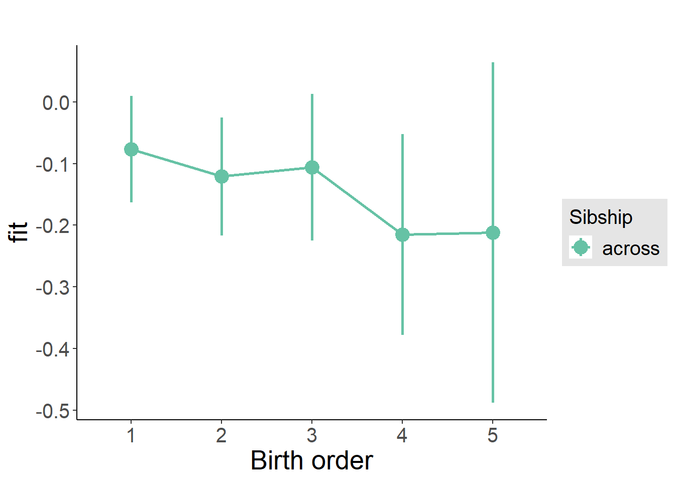
Add Interaction
Model Summary
m4_interaction = update(m3_birthorder_nonlinear, formula = . ~ . - birth_order_nonlinear - sibling_count + count_birth_order)
tidy(m4_interaction, conf.int = T, conf.level = 0.995)| effect | group | term | estimate | std.error | statistic | df | p.value | conf.low | conf.high |
|---|---|---|---|---|---|---|---|---|---|
| fixed | NA | (Intercept) | -0.7424 | 0.5583 | -1.33 | 4471 | 0.1837 | -2.31 | 0.8249 |
| fixed | NA | poly(age, 3, raw = TRUE)1 | 0.006954 | 0.06518 | 0.1067 | 4466 | 0.915 | -0.176 | 0.1899 |
| fixed | NA | poly(age, 3, raw = TRUE)2 | 0.001458 | 0.002405 | 0.6061 | 4460 | 0.5445 | -0.005293 | 0.008208 |
| fixed | NA | poly(age, 3, raw = TRUE)3 | -0.00002354 | 0.00002823 | -0.8338 | 4453 | 0.4044 | -0.0001028 | 0.0000557 |
| fixed | NA | male | 0.0423 | 0.02987 | 1.416 | 4452 | 0.1569 | -0.04155 | 0.1261 |
| fixed | NA | count_birth_order2/2 | -0.09533 | 0.05977 | -1.595 | 3740 | 0.1108 | -0.2631 | 0.07245 |
| fixed | NA | count_birth_order1/3 | -0.03278 | 0.05295 | -0.619 | 4471 | 0.5359 | -0.1814 | 0.1159 |
| fixed | NA | count_birth_order2/3 | -0.1422 | 0.05857 | -2.427 | 4475 | 0.01525 | -0.3066 | 0.02224 |
| fixed | NA | count_birth_order3/3 | -0.1568 | 0.06438 | -2.436 | 4471 | 0.01491 | -0.3375 | 0.02392 |
| fixed | NA | count_birth_order1/4 | -0.1093 | 0.06608 | -1.655 | 4473 | 0.09804 | -0.2948 | 0.07614 |
| fixed | NA | count_birth_order2/4 | -0.03314 | 0.06789 | -0.4881 | 4475 | 0.6255 | -0.2237 | 0.1574 |
| fixed | NA | count_birth_order3/4 | -0.02125 | 0.07111 | -0.2989 | 4467 | 0.7651 | -0.2209 | 0.1784 |
| fixed | NA | count_birth_order4/4 | -0.2189 | 0.07512 | -2.914 | 4464 | 0.003591 | -0.4298 | -0.008005 |
| fixed | NA | count_birth_order1/5 | -0.09137 | 0.0893 | -1.023 | 4475 | 0.3063 | -0.342 | 0.1593 |
| fixed | NA | count_birth_order2/5 | 0.0628 | 0.09856 | 0.6372 | 4469 | 0.524 | -0.2139 | 0.3395 |
| fixed | NA | count_birth_order3/5 | 0.04785 | 0.09394 | 0.5094 | 4464 | 0.6105 | -0.2158 | 0.3115 |
| fixed | NA | count_birth_order4/5 | -0.03201 | 0.09046 | -0.3539 | 4464 | 0.7234 | -0.2859 | 0.2219 |
| fixed | NA | count_birth_order5/5 | -0.08909 | 0.09607 | -0.9272 | 4459 | 0.3538 | -0.3588 | 0.1806 |
| ran_pars | mother_pidlink | sd__(Intercept) | 0.2364 | NA | NA | NA | NA | NA | NA |
| ran_pars | Residual | sd__Observation | 0.9715 | NA | NA | NA | NA | NA | NA |
Coefficient Plot
plot_birthorder(m4_interaction)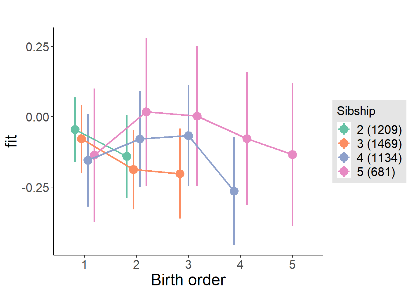
Model Comparison
###### Model 1 - Model 2
anova(m1_covariates_only, m2_birthorder_linear, m3_birthorder_nonlinear, m4_interaction)## refitting model(s) with ML (instead of REML)| Df | AIC | BIC | logLik | deviance | Chisq | Chi Df | Pr(>Chisq) |
|---|---|---|---|---|---|---|---|
| 10 | 12762 | 12826 | -6371 | 12742 | NA | NA | NA |
| 11 | 12760 | 12830 | -6369 | 12738 | 4.342 | 1 | 0.03719 |
| 14 | 12764 | 12854 | -6368 | 12736 | 1.716 | 3 | 0.6335 |
| 20 | 12765 | 12894 | -6363 | 12725 | 10.69 | 6 | 0.09841 |
Compare birth order specifications
library(coefplot)
multiplot(outcome_naive_m1, outcome_preg_m1, outcome_uterus_m1, outcome_parental_m1, dodgeHeight = 0.6,
intercept = FALSE)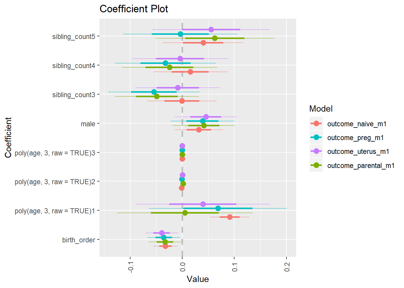
Agreeableness
birthorder <- birthorder %>% mutate(outcome = big5_agree)
model = lmer(outcome ~ birth_order + poly(age, 3, raw = TRUE) + male + sibling_count + (1 | mother_pidlink),
data = birthorder)
compare_birthorder_specs(model)Naive birth order
outcome_naive_m1 <- update(m2_birthorder_linear, data = birthorder %>%
mutate(sibling_count = sibling_count_naive_factor,
birth_order_nonlinear = birthorder_naive_factor,
birth_order = birthorder_naive,
count_birth_order = count_birthorder_naive) %>%
filter(sibling_count != "1"))
compare_models_markdown(outcome_naive_m1)Basic Model
Model Summary
m1_covariates_only <- update(m2_birthorder_linear, formula = . ~ . - birth_order)
tidy(m1_covariates_only, conf.int = T, conf.level = 0.995)| effect | group | term | estimate | std.error | statistic | df | p.value | conf.low | conf.high |
|---|---|---|---|---|---|---|---|---|---|
| fixed | NA | (Intercept) | -0.6396 | 0.2026 | -3.157 | 6657 | 0.0016 | -1.208 | -0.07095 |
| fixed | NA | poly(age, 3, raw = TRUE)1 | 0.03037 | 0.01945 | 1.562 | 6461 | 0.1184 | -0.02423 | 0.08497 |
| fixed | NA | poly(age, 3, raw = TRUE)2 | -0.000251 | 0.0005678 | -0.442 | 6245 | 0.6585 | -0.001845 | 0.001343 |
| fixed | NA | poly(age, 3, raw = TRUE)3 | -0.000001566 | 0.00000515 | -0.3042 | 6082 | 0.761 | -0.00001602 | 0.00001289 |
| fixed | NA | male | 0.08125 | 0.02368 | 3.431 | 7076 | 0.0006058 | 0.01477 | 0.1477 |
| fixed | NA | sibling_count3 | -0.02006 | 0.03366 | -0.5959 | 4930 | 0.5513 | -0.1145 | 0.07442 |
| fixed | NA | sibling_count4 | 0.02959 | 0.03464 | 0.8544 | 4330 | 0.3929 | -0.06763 | 0.1268 |
| fixed | NA | sibling_count5 | 0.005736 | 0.03595 | 0.1595 | 3704 | 0.8733 | -0.09519 | 0.1067 |
| ran_pars | mother_pidlink | sd__(Intercept) | 0.265 | NA | NA | NA | NA | NA | NA |
| ran_pars | Residual | sd__Observation | 0.9662 | NA | NA | NA | NA | NA | NA |
Coefficient Plot
plot(allEffects(m1_covariates_only, confidence.level = 0.995))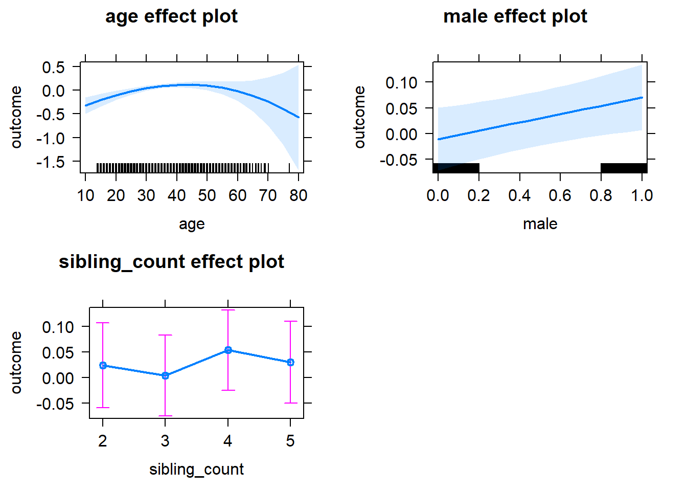
Add Birth Order Linear
Model Summary
tidy(m2_birthorder_linear, conf.int = T, conf.level = 0.995)| effect | group | term | estimate | std.error | statistic | df | p.value | conf.low | conf.high |
|---|---|---|---|---|---|---|---|---|---|
| fixed | NA | (Intercept) | -0.6382 | 0.2026 | -3.149 | 6646 | 0.001643 | -1.207 | -0.06939 |
| fixed | NA | birth_order | -0.004159 | 0.01187 | -0.3504 | 6119 | 0.726 | -0.03747 | 0.02916 |
| fixed | NA | poly(age, 3, raw = TRUE)1 | 0.03079 | 0.01949 | 1.58 | 6489 | 0.1141 | -0.02391 | 0.0855 |
| fixed | NA | poly(age, 3, raw = TRUE)2 | -0.0002616 | 0.0005686 | -0.4601 | 6261 | 0.6455 | -0.001858 | 0.001335 |
| fixed | NA | poly(age, 3, raw = TRUE)3 | -0.000001497 | 0.000005154 | -0.2905 | 6090 | 0.7715 | -0.00001596 | 0.00001297 |
| fixed | NA | male | 0.08137 | 0.02369 | 3.435 | 7074 | 0.0005957 | 0.01488 | 0.1479 |
| fixed | NA | sibling_count3 | -0.01856 | 0.03393 | -0.5471 | 5066 | 0.5844 | -0.1138 | 0.07668 |
| fixed | NA | sibling_count4 | 0.03307 | 0.03603 | 0.9178 | 4904 | 0.3588 | -0.06807 | 0.1342 |
| fixed | NA | sibling_count5 | 0.01131 | 0.03932 | 0.2876 | 4847 | 0.7736 | -0.09907 | 0.1217 |
| ran_pars | mother_pidlink | sd__(Intercept) | 0.2652 | NA | NA | NA | NA | NA | NA |
| ran_pars | Residual | sd__Observation | 0.9663 | NA | NA | NA | NA | NA | NA |
Coefficient Plot
plot_birthorder2(m2_birthorder_linear, separate = FALSE)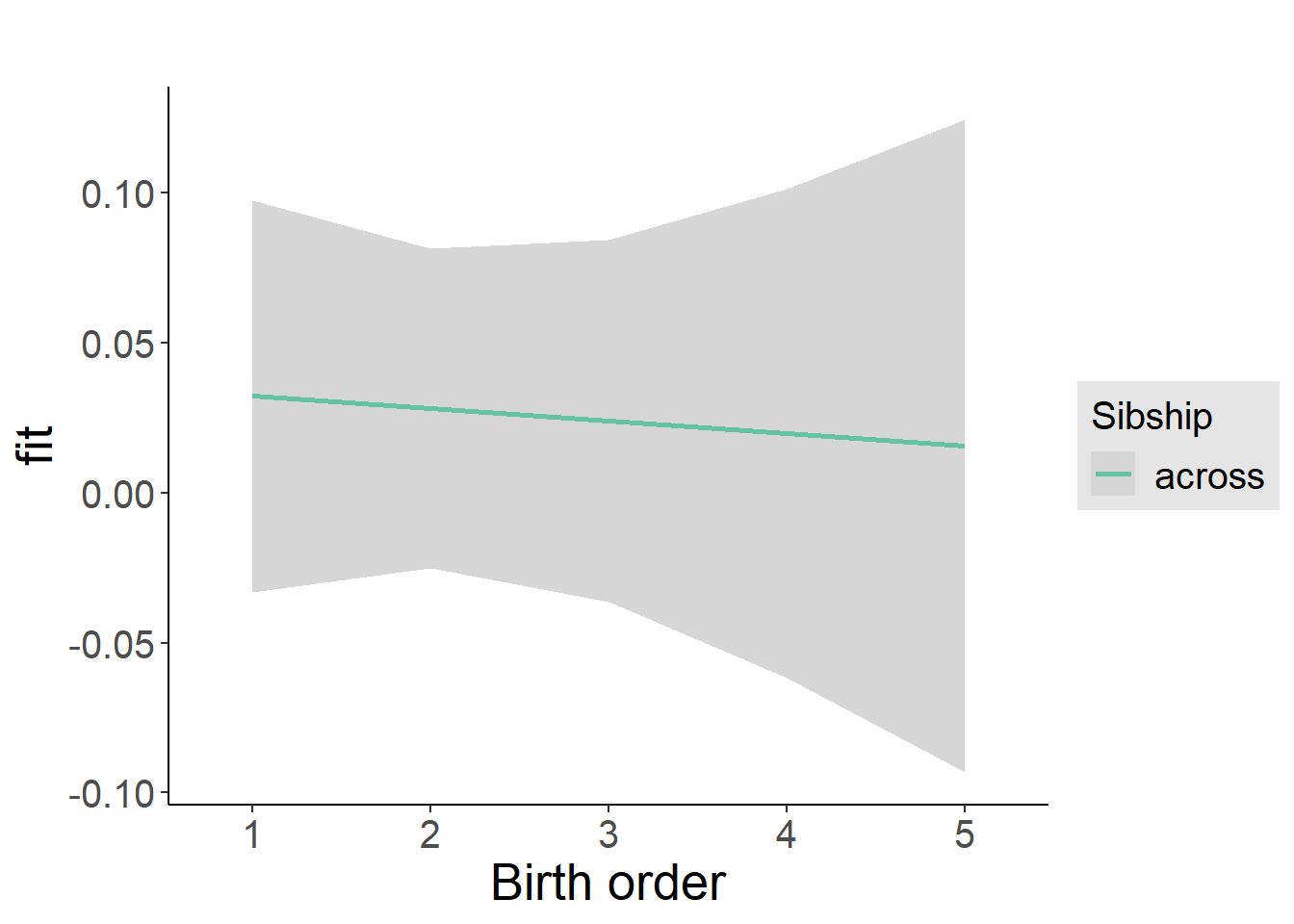
Add Birth Order Factor
Model Summary
m3_birthorder_nonlinear = update(m1_covariates_only, formula = . ~ . + birth_order_nonlinear)
tidy(m3_birthorder_nonlinear, conf.int = T, conf.level = 0.995)| effect | group | term | estimate | std.error | statistic | df | p.value | conf.low | conf.high |
|---|---|---|---|---|---|---|---|---|---|
| fixed | NA | (Intercept) | -0.6372 | 0.2032 | -3.136 | 6674 | 0.001721 | -1.208 | -0.06682 |
| fixed | NA | poly(age, 3, raw = TRUE)1 | 0.03043 | 0.0195 | 1.561 | 6477 | 0.1187 | -0.0243 | 0.08516 |
| fixed | NA | poly(age, 3, raw = TRUE)2 | -0.0002432 | 0.000569 | -0.4274 | 6239 | 0.6691 | -0.00184 | 0.001354 |
| fixed | NA | poly(age, 3, raw = TRUE)3 | -0.00000173 | 0.000005159 | -0.3352 | 6056 | 0.7375 | -0.00001621 | 0.00001275 |
| fixed | NA | male | 0.08145 | 0.02368 | 3.439 | 7070 | 0.0005871 | 0.01497 | 0.1479 |
| fixed | NA | sibling_count3 | -0.006306 | 0.03449 | -0.1829 | 5292 | 0.8549 | -0.1031 | 0.0905 |
| fixed | NA | sibling_count4 | 0.0369 | 0.03665 | 1.007 | 5161 | 0.314 | -0.06597 | 0.1398 |
| fixed | NA | sibling_count5 | 0.009944 | 0.03972 | 0.2503 | 5035 | 0.8023 | -0.1015 | 0.1214 |
| fixed | NA | birth_order_nonlinear2 | -0.01421 | 0.02821 | -0.5037 | 5966 | 0.6145 | -0.09338 | 0.06497 |
| fixed | NA | birth_order_nonlinear3 | -0.06549 | 0.0362 | -1.809 | 5946 | 0.07049 | -0.1671 | 0.03613 |
| fixed | NA | birth_order_nonlinear4 | 0.02726 | 0.04728 | 0.5766 | 5967 | 0.5643 | -0.1055 | 0.16 |
| fixed | NA | birth_order_nonlinear5 | 0.008859 | 0.06881 | 0.1287 | 5857 | 0.8976 | -0.1843 | 0.202 |
| ran_pars | mother_pidlink | sd__(Intercept) | 0.2661 | NA | NA | NA | NA | NA | NA |
| ran_pars | Residual | sd__Observation | 0.9659 | NA | NA | NA | NA | NA | NA |
Coefficient Plot
plot_birthorder(m3_birthorder_nonlinear, separate = FALSE)
Add Interaction
Model Summary
m4_interaction = update(m3_birthorder_nonlinear, formula = . ~ . - birth_order_nonlinear - sibling_count + count_birth_order)
tidy(m4_interaction, conf.int = T, conf.level = 0.995)| effect | group | term | estimate | std.error | statistic | df | p.value | conf.low | conf.high |
|---|---|---|---|---|---|---|---|---|---|
| fixed | NA | (Intercept) | -0.6303 | 0.2037 | -3.095 | 6681 | 0.001978 | -1.202 | -0.05859 |
| fixed | NA | poly(age, 3, raw = TRUE)1 | 0.03066 | 0.0195 | 1.572 | 6477 | 0.116 | -0.02409 | 0.08541 |
| fixed | NA | poly(age, 3, raw = TRUE)2 | -0.0002451 | 0.0005692 | -0.4306 | 6235 | 0.6668 | -0.001843 | 0.001353 |
| fixed | NA | poly(age, 3, raw = TRUE)3 | -0.000001756 | 0.000005161 | -0.3403 | 6049 | 0.7337 | -0.00001624 | 0.00001273 |
| fixed | NA | male | 0.08157 | 0.02369 | 3.443 | 7062 | 0.000579 | 0.01506 | 0.1481 |
| fixed | NA | count_birth_order2/2 | -0.04349 | 0.04814 | -0.9035 | 5891 | 0.3663 | -0.1786 | 0.09163 |
| fixed | NA | count_birth_order1/3 | -0.0283 | 0.04522 | -0.6258 | 7116 | 0.5315 | -0.1552 | 0.09864 |
| fixed | NA | count_birth_order2/3 | 0.002456 | 0.05058 | 0.04856 | 7126 | 0.9613 | -0.1395 | 0.1444 |
| fixed | NA | count_birth_order3/3 | -0.1075 | 0.05672 | -1.895 | 7129 | 0.05807 | -0.2667 | 0.05171 |
| fixed | NA | count_birth_order1/4 | -0.002901 | 0.05167 | -0.05614 | 7127 | 0.9552 | -0.1479 | 0.1421 |
| fixed | NA | count_birth_order2/4 | 0.0132 | 0.05435 | 0.2429 | 7128 | 0.8081 | -0.1394 | 0.1658 |
| fixed | NA | count_birth_order3/4 | -0.03154 | 0.05909 | -0.5337 | 7128 | 0.5935 | -0.1974 | 0.1343 |
| fixed | NA | count_birth_order4/4 | 0.09117 | 0.06261 | 1.456 | 7125 | 0.1454 | -0.08459 | 0.2669 |
| fixed | NA | count_birth_order1/5 | 0.03404 | 0.05866 | 0.5804 | 7129 | 0.5617 | -0.1306 | 0.1987 |
| fixed | NA | count_birth_order2/5 | -0.04159 | 0.06173 | -0.6738 | 7125 | 0.5005 | -0.2149 | 0.1317 |
| fixed | NA | count_birth_order3/5 | -0.04275 | 0.06338 | -0.6745 | 7123 | 0.5 | -0.2207 | 0.1352 |
| fixed | NA | count_birth_order4/5 | -0.01951 | 0.06718 | -0.2904 | 7118 | 0.7715 | -0.2081 | 0.1691 |
| fixed | NA | count_birth_order5/5 | 0.007504 | 0.06868 | 0.1093 | 7116 | 0.913 | -0.1853 | 0.2003 |
| ran_pars | mother_pidlink | sd__(Intercept) | 0.2671 | NA | NA | NA | NA | NA | NA |
| ran_pars | Residual | sd__Observation | 0.9658 | NA | NA | NA | NA | NA | NA |
Coefficient Plot
plot_birthorder(m4_interaction)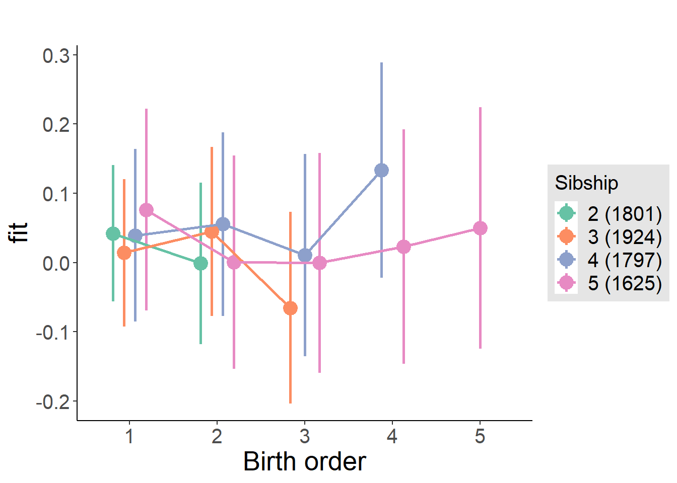
Model Comparison
###### Model 1 - Model 2
anova(m1_covariates_only, m2_birthorder_linear, m3_birthorder_nonlinear, m4_interaction)## refitting model(s) with ML (instead of REML)| Df | AIC | BIC | logLik | deviance | Chisq | Chi Df | Pr(>Chisq) |
|---|---|---|---|---|---|---|---|
| 10 | 20306 | 20374 | -10143 | 20286 | NA | NA | NA |
| 11 | 20308 | 20383 | -10143 | 20286 | 0.1222 | 1 | 0.7266 |
| 14 | 20309 | 20405 | -10140 | 20281 | 4.63 | 3 | 0.201 |
| 20 | 20317 | 20454 | -10138 | 20277 | 4.042 | 6 | 0.671 |
Maternal birth order
outcome_uterus_m1 <- update(m2_birthorder_linear, data = birthorder %>%
mutate(sibling_count = sibling_count_uterus_alive_factor,
birth_order_nonlinear = birthorder_uterus_alive_factor,
birth_order = birthorder_uterus_alive,
count_birth_order = count_birthorder_uterus_alive) %>%
filter(sibling_count != "1"))
compare_models_markdown(outcome_uterus_m1)Basic Model
Model Summary
m1_covariates_only <- update(m2_birthorder_linear, formula = . ~ . - birth_order)
tidy(m1_covariates_only, conf.int = T, conf.level = 0.995)| effect | group | term | estimate | std.error | statistic | df | p.value | conf.low | conf.high |
|---|---|---|---|---|---|---|---|---|---|
| fixed | NA | (Intercept) | -1.5 | 0.5476 | -2.739 | 4500 | 0.00619 | -3.037 | 0.03735 |
| fixed | NA | poly(age, 3, raw = TRUE)1 | 0.1335 | 0.06391 | 2.089 | 4500 | 0.03676 | -0.04588 | 0.3129 |
| fixed | NA | poly(age, 3, raw = TRUE)2 | -0.004014 | 0.002355 | -1.704 | 4498 | 0.08838 | -0.01062 | 0.002597 |
| fixed | NA | poly(age, 3, raw = TRUE)3 | 0.00004243 | 0.00002759 | 1.538 | 4494 | 0.1241 | -0.00003501 | 0.0001199 |
| fixed | NA | male | 0.06132 | 0.0295 | 2.078 | 4451 | 0.03772 | -0.0215 | 0.1441 |
| fixed | NA | sibling_count3 | -0.04346 | 0.04011 | -1.084 | 3284 | 0.2786 | -0.156 | 0.06912 |
| fixed | NA | sibling_count4 | -0.05491 | 0.04325 | -1.27 | 2832 | 0.2044 | -0.1763 | 0.0665 |
| fixed | NA | sibling_count5 | 0.003817 | 0.04932 | 0.07739 | 2478 | 0.9383 | -0.1346 | 0.1423 |
| ran_pars | mother_pidlink | sd__(Intercept) | 0.3084 | NA | NA | NA | NA | NA | NA |
| ran_pars | Residual | sd__Observation | 0.9439 | NA | NA | NA | NA | NA | NA |
Coefficient Plot
plot(allEffects(m1_covariates_only, confidence.level = 0.995))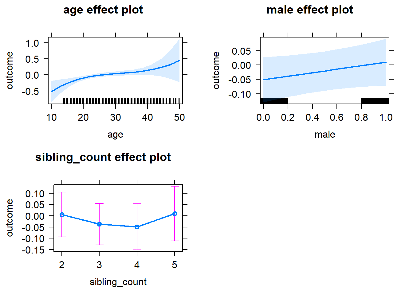
Add Birth Order Linear
Model Summary
tidy(m2_birthorder_linear, conf.int = T, conf.level = 0.995)| effect | group | term | estimate | std.error | statistic | df | p.value | conf.low | conf.high |
|---|---|---|---|---|---|---|---|---|---|
| fixed | NA | (Intercept) | -1.5 | 0.5483 | -2.736 | 4499 | 0.006243 | -3.039 | 0.03894 |
| fixed | NA | birth_order | 0.0002383 | 0.0155 | 0.01537 | 4179 | 0.9877 | -0.04327 | 0.04375 |
| fixed | NA | poly(age, 3, raw = TRUE)1 | 0.1335 | 0.06392 | 2.089 | 4499 | 0.03678 | -0.04591 | 0.3129 |
| fixed | NA | poly(age, 3, raw = TRUE)2 | -0.004014 | 0.002356 | -1.704 | 4497 | 0.08845 | -0.01063 | 0.002598 |
| fixed | NA | poly(age, 3, raw = TRUE)3 | 0.00004244 | 0.00002761 | 1.537 | 4494 | 0.1243 | -0.00003505 | 0.0001199 |
| fixed | NA | male | 0.06132 | 0.02951 | 2.078 | 4450 | 0.03779 | -0.02152 | 0.1442 |
| fixed | NA | sibling_count3 | -0.04357 | 0.04073 | -1.07 | 3348 | 0.2848 | -0.1579 | 0.07077 |
| fixed | NA | sibling_count4 | -0.05516 | 0.04624 | -1.193 | 3071 | 0.233 | -0.185 | 0.07463 |
| fixed | NA | sibling_count5 | 0.003396 | 0.05639 | 0.06022 | 3013 | 0.952 | -0.1549 | 0.1617 |
| ran_pars | mother_pidlink | sd__(Intercept) | 0.3083 | NA | NA | NA | NA | NA | NA |
| ran_pars | Residual | sd__Observation | 0.944 | NA | NA | NA | NA | NA | NA |
Coefficient Plot
plot_birthorder2(m2_birthorder_linear, separate = FALSE)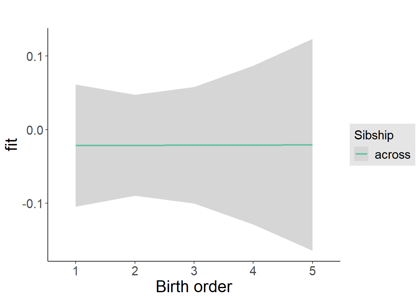
Add Birth Order Factor
Model Summary
m3_birthorder_nonlinear = update(m1_covariates_only, formula = . ~ . + birth_order_nonlinear)
tidy(m3_birthorder_nonlinear, conf.int = T, conf.level = 0.995)| effect | group | term | estimate | std.error | statistic | df | p.value | conf.low | conf.high |
|---|---|---|---|---|---|---|---|---|---|
| fixed | NA | (Intercept) | -1.441 | 0.5487 | -2.626 | 4496 | 0.008657 | -2.982 | 0.09909 |
| fixed | NA | poly(age, 3, raw = TRUE)1 | 0.1283 | 0.06398 | 2.006 | 4495 | 0.04497 | -0.05128 | 0.3079 |
| fixed | NA | poly(age, 3, raw = TRUE)2 | -0.003825 | 0.002358 | -1.622 | 4492 | 0.1048 | -0.01044 | 0.002793 |
| fixed | NA | poly(age, 3, raw = TRUE)3 | 0.00004036 | 0.00002763 | 1.461 | 4489 | 0.1441 | -0.00003719 | 0.0001179 |
| fixed | NA | male | 0.06081 | 0.02952 | 2.06 | 4447 | 0.03942 | -0.02204 | 0.1437 |
| fixed | NA | sibling_count3 | -0.03525 | 0.04137 | -0.852 | 3473 | 0.3943 | -0.1514 | 0.08088 |
| fixed | NA | sibling_count4 | -0.04977 | 0.04693 | -1.061 | 3176 | 0.289 | -0.1815 | 0.08197 |
| fixed | NA | sibling_count5 | -0.01692 | 0.05735 | -0.295 | 3105 | 0.768 | -0.1779 | 0.1441 |
| fixed | NA | birth_order_nonlinear2 | -0.04439 | 0.03521 | -1.261 | 3616 | 0.2075 | -0.1432 | 0.05445 |
| fixed | NA | birth_order_nonlinear3 | -0.03947 | 0.04486 | -0.8798 | 3847 | 0.379 | -0.1654 | 0.08646 |
| fixed | NA | birth_order_nonlinear4 | 0.0003313 | 0.06023 | 0.005502 | 4043 | 0.9956 | -0.1687 | 0.1694 |
| fixed | NA | birth_order_nonlinear5 | 0.1025 | 0.0938 | 1.092 | 3913 | 0.2748 | -0.1608 | 0.3657 |
| ran_pars | mother_pidlink | sd__(Intercept) | 0.3076 | NA | NA | NA | NA | NA | NA |
| ran_pars | Residual | sd__Observation | 0.9441 | NA | NA | NA | NA | NA | NA |
Coefficient Plot
plot_birthorder(m3_birthorder_nonlinear, separate = FALSE)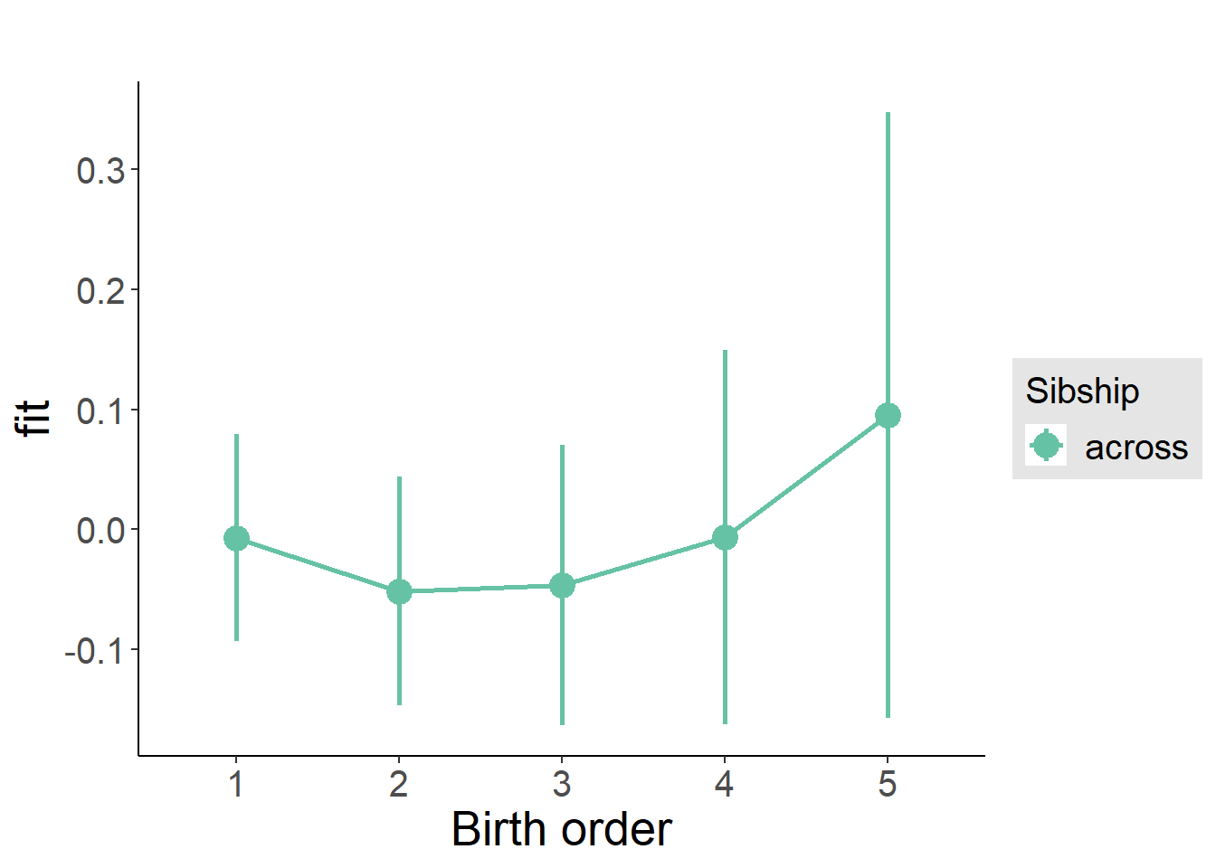
Add Interaction
Model Summary
m4_interaction = update(m3_birthorder_nonlinear, formula = . ~ . - birth_order_nonlinear - sibling_count + count_birth_order)
tidy(m4_interaction, conf.int = T, conf.level = 0.995)| effect | group | term | estimate | std.error | statistic | df | p.value | conf.low | conf.high |
|---|---|---|---|---|---|---|---|---|---|
| fixed | NA | (Intercept) | -1.441 | 0.5491 | -2.624 | 4490 | 0.00872 | -2.982 | 0.1005 |
| fixed | NA | poly(age, 3, raw = TRUE)1 | 0.1278 | 0.06402 | 1.996 | 4489 | 0.04596 | -0.0519 | 0.3075 |
| fixed | NA | poly(age, 3, raw = TRUE)2 | -0.003799 | 0.00236 | -1.61 | 4487 | 0.1075 | -0.01042 | 0.002825 |
| fixed | NA | poly(age, 3, raw = TRUE)3 | 0.00003998 | 0.00002765 | 1.446 | 4484 | 0.1483 | -0.00003764 | 0.0001176 |
| fixed | NA | male | 0.06115 | 0.02954 | 2.07 | 4440 | 0.03851 | -0.02177 | 0.1441 |
| fixed | NA | count_birth_order2/2 | -0.03908 | 0.06043 | -0.6467 | 3794 | 0.5179 | -0.2087 | 0.1306 |
| fixed | NA | count_birth_order1/3 | -0.03174 | 0.05322 | -0.5964 | 4483 | 0.551 | -0.1811 | 0.1177 |
| fixed | NA | count_birth_order2/3 | -0.05728 | 0.05814 | -0.9852 | 4490 | 0.3246 | -0.2205 | 0.1059 |
| fixed | NA | count_birth_order3/3 | -0.1057 | 0.065 | -1.627 | 4486 | 0.1039 | -0.2882 | 0.07672 |
| fixed | NA | count_birth_order1/4 | -0.07014 | 0.06529 | -1.074 | 4487 | 0.2828 | -0.2534 | 0.1131 |
| fixed | NA | count_birth_order2/4 | -0.1093 | 0.06747 | -1.62 | 4490 | 0.1054 | -0.2987 | 0.08011 |
| fixed | NA | count_birth_order3/4 | -0.06472 | 0.07125 | -0.9083 | 4478 | 0.3637 | -0.2647 | 0.1353 |
| fixed | NA | count_birth_order4/4 | -0.01905 | 0.07401 | -0.2574 | 4476 | 0.7969 | -0.2268 | 0.1887 |
| fixed | NA | count_birth_order1/5 | 0.03532 | 0.08881 | 0.3977 | 4487 | 0.6909 | -0.214 | 0.2846 |
| fixed | NA | count_birth_order2/5 | -0.1062 | 0.09483 | -1.12 | 4471 | 0.2627 | -0.3724 | 0.16 |
| fixed | NA | count_birth_order3/5 | -0.02283 | 0.08884 | -0.257 | 4466 | 0.7972 | -0.2722 | 0.2265 |
| fixed | NA | count_birth_order4/5 | -0.05543 | 0.08553 | -0.6481 | 4471 | 0.517 | -0.2955 | 0.1847 |
| fixed | NA | count_birth_order5/5 | 0.08677 | 0.08895 | 0.9754 | 4459 | 0.3294 | -0.1629 | 0.3365 |
| ran_pars | mother_pidlink | sd__(Intercept) | 0.3084 | NA | NA | NA | NA | NA | NA |
| ran_pars | Residual | sd__Observation | 0.9443 | NA | NA | NA | NA | NA | NA |
Coefficient Plot
plot_birthorder(m4_interaction)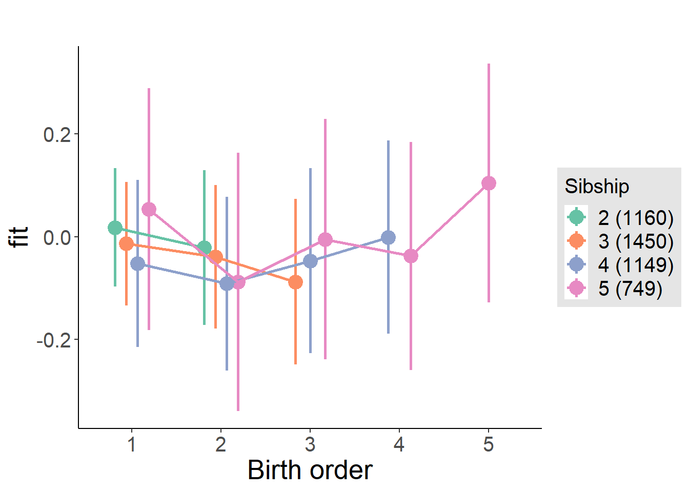
Model Comparison
###### Model 1 - Model 2
anova(m1_covariates_only, m2_birthorder_linear, m3_birthorder_nonlinear, m4_interaction)## refitting model(s) with ML (instead of REML)| Df | AIC | BIC | logLik | deviance | Chisq | Chi Df | Pr(>Chisq) |
|---|---|---|---|---|---|---|---|
| 10 | 12726 | 12790 | -6353 | 12706 | NA | NA | NA |
| 11 | 12728 | 12798 | -6353 | 12706 | 0.0002465 | 1 | 0.9875 |
| 14 | 12730 | 12819 | -6351 | 12702 | 3.899 | 3 | 0.2726 |
| 20 | 12739 | 12868 | -6350 | 12699 | 2.374 | 6 | 0.8823 |
Maternal pregnancy order
outcome_preg_m1 <- update(m2_birthorder_linear, data = birthorder %>%
mutate(sibling_count = sibling_count_uterus_preg_factor,
birth_order_nonlinear = birthorder_uterus_preg_factor,
birth_order = birthorder_uterus_preg,
count_birth_order = count_birthorder_uterus_preg
) %>%
filter(sibling_count != "1"))
compare_models_markdown(outcome_preg_m1)Basic Model
Model Summary
m1_covariates_only <- update(m2_birthorder_linear, formula = . ~ . - birth_order)
tidy(m1_covariates_only, conf.int = T, conf.level = 0.995)| effect | group | term | estimate | std.error | statistic | df | p.value | conf.low | conf.high |
|---|---|---|---|---|---|---|---|---|---|
| fixed | NA | (Intercept) | -1.622 | 0.5615 | -2.889 | 4176 | 0.003883 | -3.198 | -0.04611 |
| fixed | NA | poly(age, 3, raw = TRUE)1 | 0.1442 | 0.06558 | 2.199 | 4177 | 0.02793 | -0.03988 | 0.3283 |
| fixed | NA | poly(age, 3, raw = TRUE)2 | -0.004261 | 0.002417 | -1.763 | 4176 | 0.07801 | -0.01105 | 0.002524 |
| fixed | NA | poly(age, 3, raw = TRUE)3 | 0.0000436 | 0.00002833 | 1.539 | 4174 | 0.1238 | -0.00003591 | 0.0001231 |
| fixed | NA | male | 0.08473 | 0.03048 | 2.78 | 4121 | 0.005467 | -0.000836 | 0.1703 |
| fixed | NA | sibling_count3 | -0.05352 | 0.04327 | -1.237 | 3135 | 0.2162 | -0.175 | 0.06794 |
| fixed | NA | sibling_count4 | -0.02786 | 0.04574 | -0.6092 | 2825 | 0.5424 | -0.1562 | 0.1005 |
| fixed | NA | sibling_count5 | -0.03858 | 0.04896 | -0.788 | 2496 | 0.4308 | -0.176 | 0.09884 |
| ran_pars | mother_pidlink | sd__(Intercept) | 0.3201 | NA | NA | NA | NA | NA | NA |
| ran_pars | Residual | sd__Observation | 0.9354 | NA | NA | NA | NA | NA | NA |
Coefficient Plot
plot(allEffects(m1_covariates_only, confidence.level = 0.995))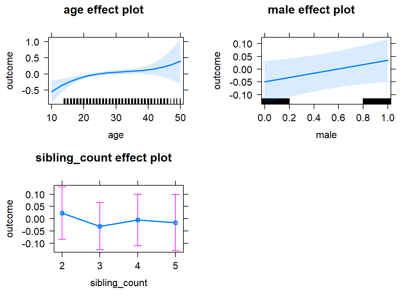
Add Birth Order Linear
Model Summary
tidy(m2_birthorder_linear, conf.int = T, conf.level = 0.995)| effect | group | term | estimate | std.error | statistic | df | p.value | conf.low | conf.high |
|---|---|---|---|---|---|---|---|---|---|
| fixed | NA | (Intercept) | -1.617 | 0.5621 | -2.876 | 4175 | 0.00405 | -3.194 | -0.03868 |
| fixed | NA | birth_order | -0.003374 | 0.01545 | -0.2184 | 3947 | 0.8271 | -0.04674 | 0.04 |
| fixed | NA | poly(age, 3, raw = TRUE)1 | 0.144 | 0.06559 | 2.196 | 4176 | 0.02816 | -0.04009 | 0.3281 |
| fixed | NA | poly(age, 3, raw = TRUE)2 | -0.004251 | 0.002418 | -1.758 | 4175 | 0.0788 | -0.01104 | 0.002536 |
| fixed | NA | poly(age, 3, raw = TRUE)3 | 0.00004342 | 0.00002834 | 1.532 | 4173 | 0.1256 | -0.00003614 | 0.000123 |
| fixed | NA | male | 0.0848 | 0.03049 | 2.782 | 4120 | 0.005435 | -0.000777 | 0.1704 |
| fixed | NA | sibling_count3 | -0.05198 | 0.04385 | -1.185 | 3180 | 0.2359 | -0.1751 | 0.0711 |
| fixed | NA | sibling_count4 | -0.02442 | 0.04837 | -0.5049 | 2999 | 0.6136 | -0.1602 | 0.1114 |
| fixed | NA | sibling_count5 | -0.03308 | 0.05505 | -0.601 | 2905 | 0.5479 | -0.1876 | 0.1214 |
| ran_pars | mother_pidlink | sd__(Intercept) | 0.3202 | NA | NA | NA | NA | NA | NA |
| ran_pars | Residual | sd__Observation | 0.9355 | NA | NA | NA | NA | NA | NA |
Coefficient Plot
plot_birthorder2(m2_birthorder_linear, separate = FALSE)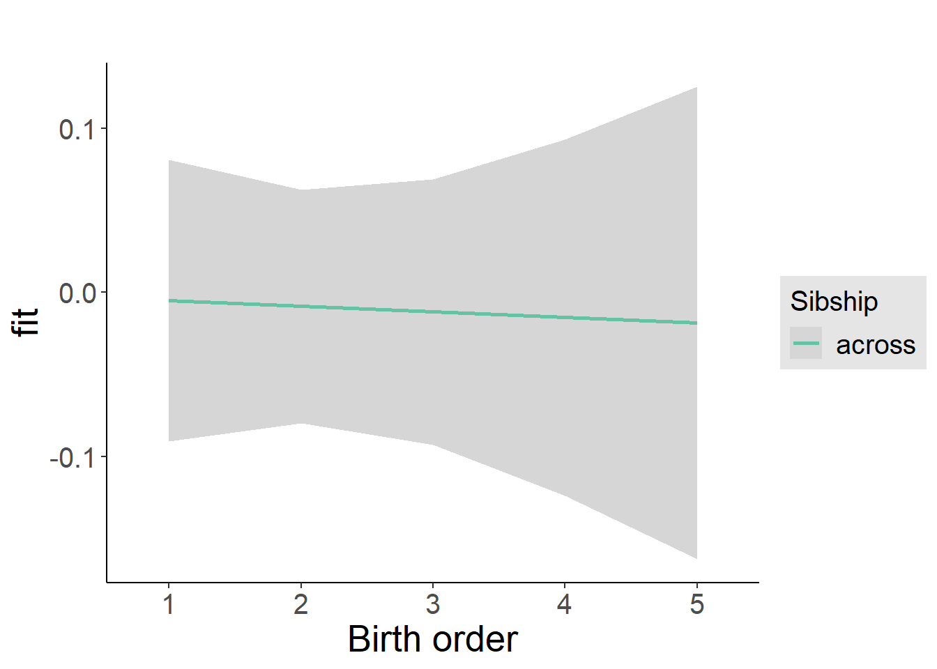
Add Birth Order Factor
Model Summary
m3_birthorder_nonlinear = update(m1_covariates_only, formula = . ~ . + birth_order_nonlinear)
tidy(m3_birthorder_nonlinear, conf.int = T, conf.level = 0.995)| effect | group | term | estimate | std.error | statistic | df | p.value | conf.low | conf.high |
|---|---|---|---|---|---|---|---|---|---|
| fixed | NA | (Intercept) | -1.576 | 0.5626 | -2.802 | 4173 | 0.005098 | -3.156 | 0.002685 |
| fixed | NA | poly(age, 3, raw = TRUE)1 | 0.1403 | 0.06565 | 2.137 | 4173 | 0.03266 | -0.04399 | 0.3246 |
| fixed | NA | poly(age, 3, raw = TRUE)2 | -0.004115 | 0.00242 | -1.7 | 4171 | 0.08916 | -0.01091 | 0.002679 |
| fixed | NA | poly(age, 3, raw = TRUE)3 | 0.00004192 | 0.00002837 | 1.478 | 4169 | 0.1395 | -0.0000377 | 0.0001215 |
| fixed | NA | male | 0.08421 | 0.0305 | 2.761 | 4117 | 0.00578 | -0.001391 | 0.1698 |
| fixed | NA | sibling_count3 | -0.04483 | 0.0445 | -1.007 | 3284 | 0.3138 | -0.1697 | 0.08009 |
| fixed | NA | sibling_count4 | -0.02207 | 0.04906 | -0.4498 | 3093 | 0.6529 | -0.1598 | 0.1157 |
| fixed | NA | sibling_count5 | -0.04252 | 0.05563 | -0.7643 | 2957 | 0.4447 | -0.1987 | 0.1136 |
| fixed | NA | birth_order_nonlinear2 | -0.03947 | 0.03643 | -1.083 | 3405 | 0.2787 | -0.1417 | 0.06279 |
| fixed | NA | birth_order_nonlinear3 | -0.04091 | 0.04606 | -0.8882 | 3630 | 0.3745 | -0.1702 | 0.08839 |
| fixed | NA | birth_order_nonlinear4 | 0.001996 | 0.06097 | 0.03275 | 3786 | 0.9739 | -0.1691 | 0.1731 |
| fixed | NA | birth_order_nonlinear5 | 0.03051 | 0.08934 | 0.3415 | 3681 | 0.7328 | -0.2203 | 0.2813 |
| ran_pars | mother_pidlink | sd__(Intercept) | 0.3202 | NA | NA | NA | NA | NA | NA |
| ran_pars | Residual | sd__Observation | 0.9356 | NA | NA | NA | NA | NA | NA |
Coefficient Plot
plot_birthorder(m3_birthorder_nonlinear, separate = FALSE)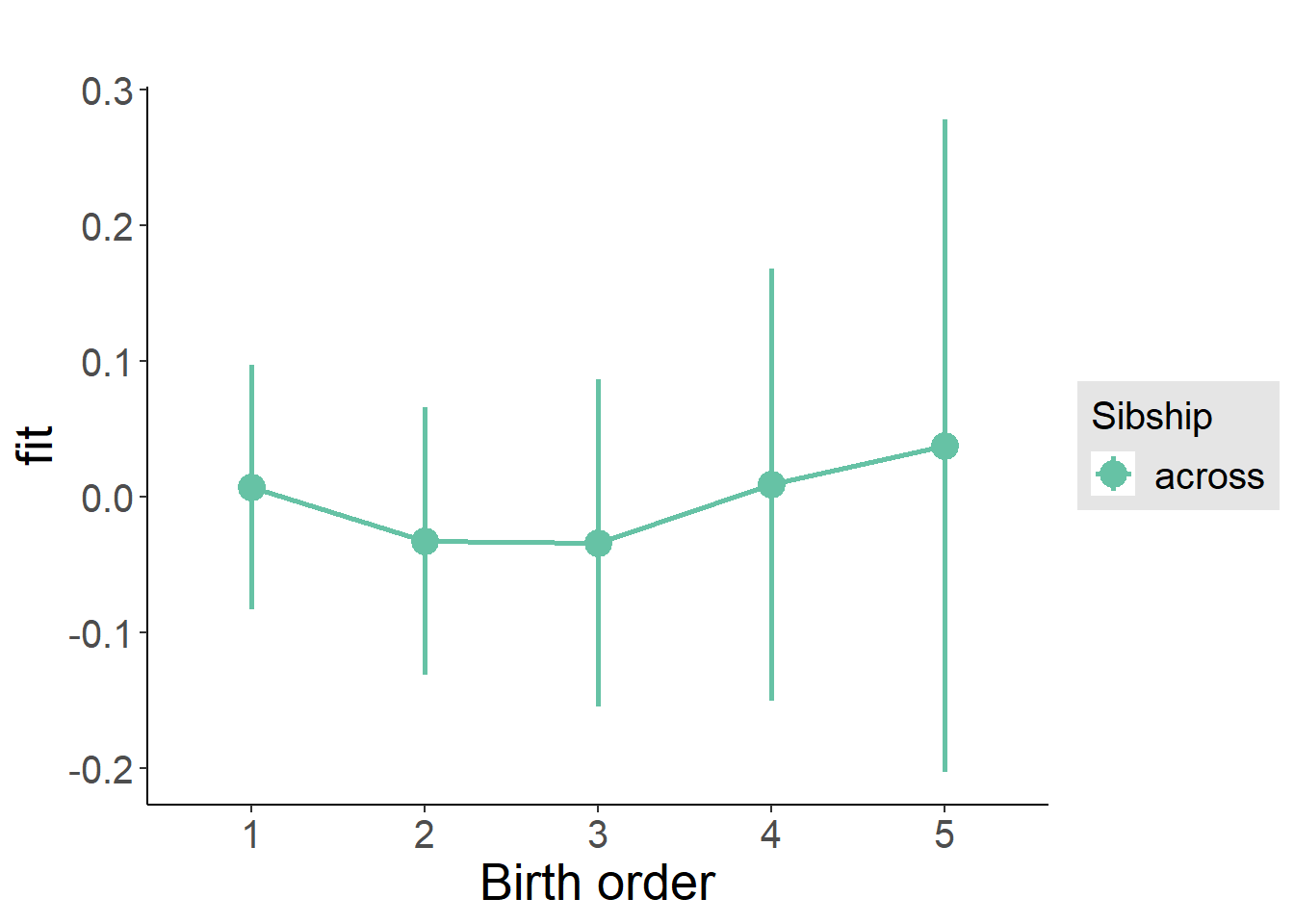
Add Interaction
Model Summary
m4_interaction = update(m3_birthorder_nonlinear, formula = . ~ . - birth_order_nonlinear - sibling_count + count_birth_order)
tidy(m4_interaction, conf.int = T, conf.level = 0.995)| effect | group | term | estimate | std.error | statistic | df | p.value | conf.low | conf.high |
|---|---|---|---|---|---|---|---|---|---|
| fixed | NA | (Intercept) | -1.573 | 0.5631 | -2.793 | 4167 | 0.005245 | -3.154 | 0.00786 |
| fixed | NA | poly(age, 3, raw = TRUE)1 | 0.141 | 0.0657 | 2.146 | 4167 | 0.03197 | -0.04346 | 0.3254 |
| fixed | NA | poly(age, 3, raw = TRUE)2 | -0.004139 | 0.002423 | -1.709 | 4165 | 0.08759 | -0.01094 | 0.002661 |
| fixed | NA | poly(age, 3, raw = TRUE)3 | 0.00004225 | 0.00002839 | 1.488 | 4163 | 0.1369 | -0.00003746 | 0.000122 |
| fixed | NA | male | 0.0846 | 0.03053 | 2.771 | 4111 | 0.005608 | -0.001091 | 0.1703 |
| fixed | NA | count_birth_order2/2 | -0.0697 | 0.06574 | -1.06 | 3567 | 0.2891 | -0.2542 | 0.1148 |
| fixed | NA | count_birth_order1/3 | -0.0591 | 0.05739 | -1.03 | 4160 | 0.3032 | -0.2202 | 0.102 |
| fixed | NA | count_birth_order2/3 | -0.06768 | 0.0622 | -1.088 | 4167 | 0.2767 | -0.2423 | 0.1069 |
| fixed | NA | count_birth_order3/3 | -0.1278 | 0.07001 | -1.825 | 4163 | 0.06804 | -0.3243 | 0.06873 |
| fixed | NA | count_birth_order1/4 | -0.05625 | 0.06811 | -0.8259 | 4164 | 0.4089 | -0.2474 | 0.1349 |
| fixed | NA | count_birth_order2/4 | -0.05083 | 0.0693 | -0.7335 | 4167 | 0.4633 | -0.2454 | 0.1437 |
| fixed | NA | count_birth_order3/4 | -0.0794 | 0.07597 | -1.045 | 4154 | 0.296 | -0.2926 | 0.1338 |
| fixed | NA | count_birth_order4/4 | -0.01828 | 0.07824 | -0.2336 | 4154 | 0.8153 | -0.2379 | 0.2013 |
| fixed | NA | count_birth_order1/5 | -0.03751 | 0.08102 | -0.463 | 4167 | 0.6434 | -0.2649 | 0.1899 |
| fixed | NA | count_birth_order2/5 | -0.1608 | 0.08677 | -1.854 | 4156 | 0.06386 | -0.4044 | 0.08273 |
| fixed | NA | count_birth_order3/5 | -0.03499 | 0.08427 | -0.4153 | 4150 | 0.678 | -0.2715 | 0.2015 |
| fixed | NA | count_birth_order4/5 | -0.06664 | 0.08727 | -0.7636 | 4136 | 0.4452 | -0.3116 | 0.1783 |
| fixed | NA | count_birth_order5/5 | -0.02222 | 0.08743 | -0.2541 | 4133 | 0.7994 | -0.2676 | 0.2232 |
| ran_pars | mother_pidlink | sd__(Intercept) | 0.3189 | NA | NA | NA | NA | NA | NA |
| ran_pars | Residual | sd__Observation | 0.9364 | NA | NA | NA | NA | NA | NA |
Coefficient Plot
plot_birthorder(m4_interaction)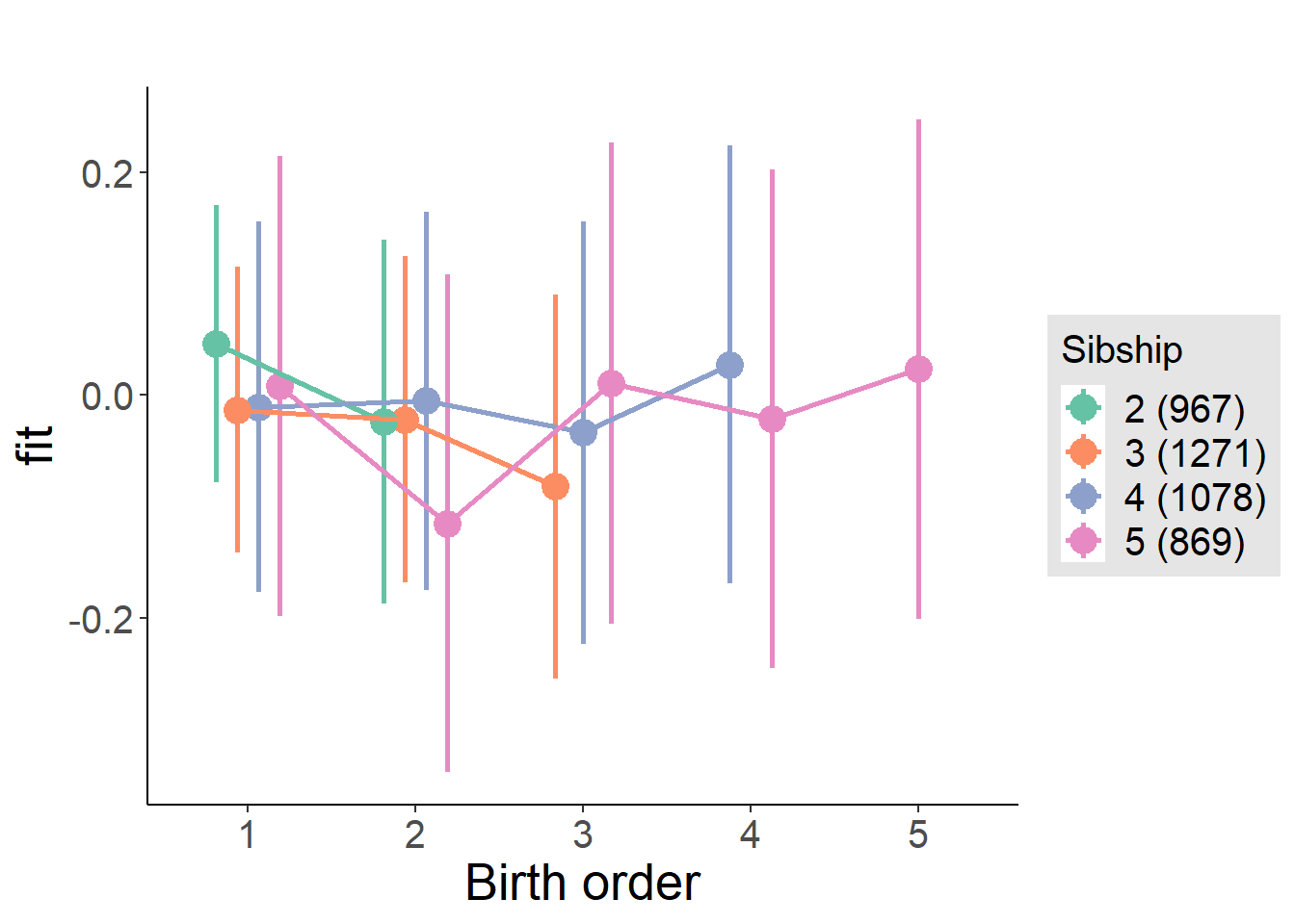
Model Comparison
###### Model 1 - Model 2
anova(m1_covariates_only, m2_birthorder_linear, m3_birthorder_nonlinear, m4_interaction)## refitting model(s) with ML (instead of REML)| Df | AIC | BIC | logLik | deviance | Chisq | Chi Df | Pr(>Chisq) |
|---|---|---|---|---|---|---|---|
| 10 | 11776 | 11840 | -5878 | 11756 | NA | NA | NA |
| 11 | 11778 | 11848 | -5878 | 11756 | 0.04759 | 1 | 0.8273 |
| 14 | 11782 | 11871 | -5877 | 11754 | 1.988 | 3 | 0.5749 |
| 20 | 11791 | 11918 | -5876 | 11751 | 2.845 | 6 | 0.8281 |
Parental full sibling order
outcome_parental_m1 <- update(m2_birthorder_linear, data = birthorder %>%
mutate(sibling_count = sibling_count_genes_factor,
birth_order_nonlinear = birthorder_genes_factor,
birth_order = birthorder_genes,
count_birth_order = count_birthorder_genes
) %>%
filter(sibling_count != "1"))
compare_models_markdown(outcome_parental_m1)Basic Model
Model Summary
m1_covariates_only <- update(m2_birthorder_linear, formula = . ~ . - birth_order)
tidy(m1_covariates_only, conf.int = T, conf.level = 0.995)| effect | group | term | estimate | std.error | statistic | df | p.value | conf.low | conf.high |
|---|---|---|---|---|---|---|---|---|---|
| fixed | NA | (Intercept) | -1.265 | 0.5515 | -2.294 | 4485 | 0.02184 | -2.813 | 0.2829 |
| fixed | NA | poly(age, 3, raw = TRUE)1 | 0.1056 | 0.06445 | 1.638 | 4484 | 0.1015 | -0.07534 | 0.2865 |
| fixed | NA | poly(age, 3, raw = TRUE)2 | -0.002981 | 0.002378 | -1.254 | 4482 | 0.21 | -0.009657 | 0.003694 |
| fixed | NA | poly(age, 3, raw = TRUE)3 | 0.00003057 | 0.00002791 | 1.095 | 4479 | 0.2734 | -0.00004778 | 0.0001089 |
| fixed | NA | male | 0.05885 | 0.0295 | 1.995 | 4438 | 0.04612 | -0.02396 | 0.1417 |
| fixed | NA | sibling_count3 | -0.04899 | 0.03949 | -1.24 | 3251 | 0.2149 | -0.1598 | 0.06187 |
| fixed | NA | sibling_count4 | -0.06476 | 0.04283 | -1.512 | 2812 | 0.1307 | -0.185 | 0.05548 |
| fixed | NA | sibling_count5 | 0.04328 | 0.05038 | 0.8591 | 2364 | 0.3904 | -0.09814 | 0.1847 |
| ran_pars | mother_pidlink | sd__(Intercept) | 0.3054 | NA | NA | NA | NA | NA | NA |
| ran_pars | Residual | sd__Observation | 0.9423 | NA | NA | NA | NA | NA | NA |
Coefficient Plot
plot(allEffects(m1_covariates_only, confidence.level = 0.995))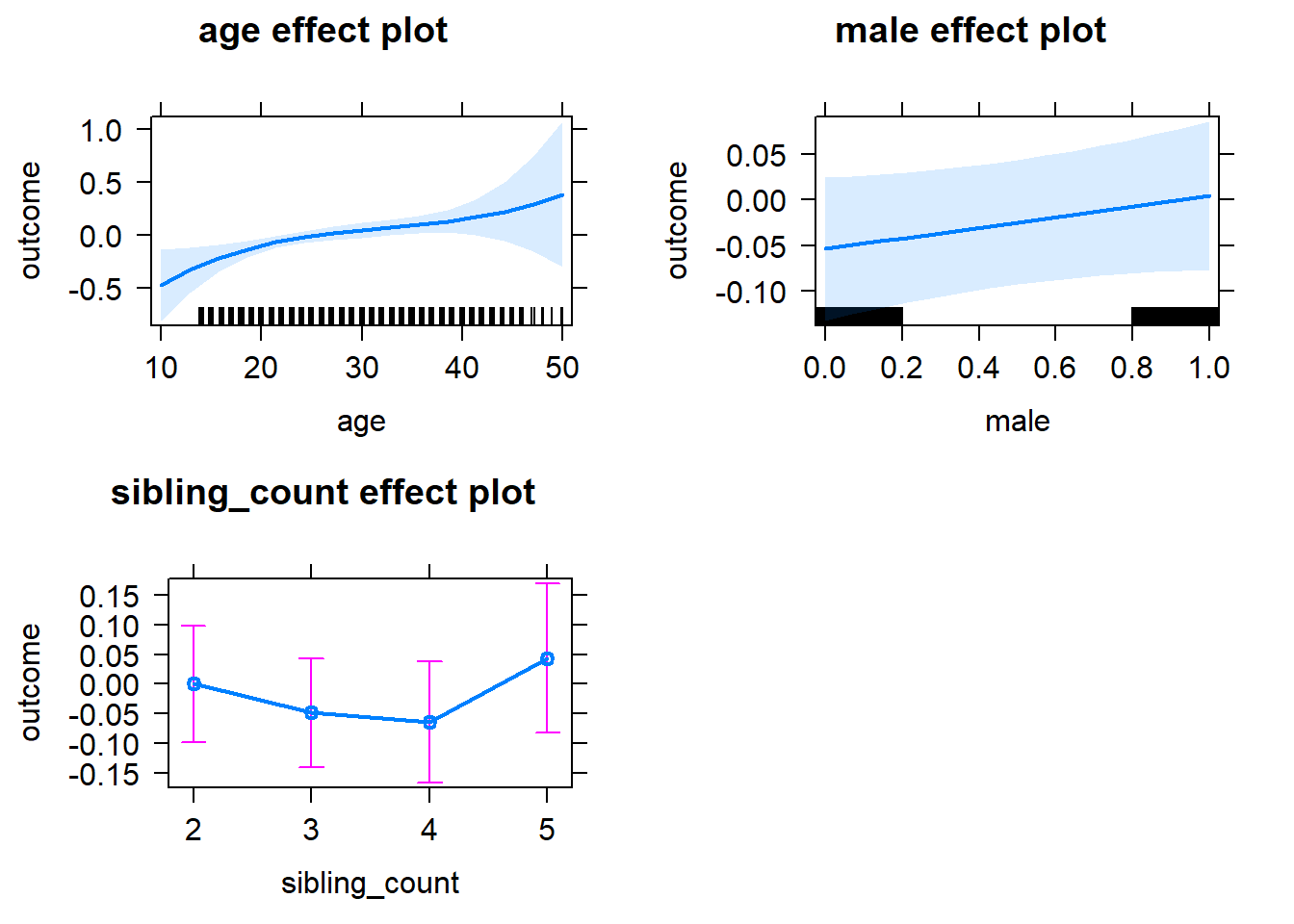
Add Birth Order Linear
Model Summary
tidy(m2_birthorder_linear, conf.int = T, conf.level = 0.995)| effect | group | term | estimate | std.error | statistic | df | p.value | conf.low | conf.high |
|---|---|---|---|---|---|---|---|---|---|
| fixed | NA | (Intercept) | -1.27 | 0.5522 | -2.3 | 4484 | 0.02151 | -2.82 | 0.2801 |
| fixed | NA | birth_order | 0.002858 | 0.01568 | 0.1823 | 4145 | 0.8553 | -0.04114 | 0.04686 |
| fixed | NA | poly(age, 3, raw = TRUE)1 | 0.1057 | 0.06446 | 1.64 | 4483 | 0.1011 | -0.07522 | 0.2867 |
| fixed | NA | poly(age, 3, raw = TRUE)2 | -0.00299 | 0.002379 | -1.257 | 4481 | 0.2088 | -0.009668 | 0.003688 |
| fixed | NA | poly(age, 3, raw = TRUE)3 | 0.00003074 | 0.00002793 | 1.1 | 4478 | 0.2712 | -0.00004767 | 0.0001091 |
| fixed | NA | male | 0.05877 | 0.02951 | 1.992 | 4436 | 0.04644 | -0.02405 | 0.1416 |
| fixed | NA | sibling_count3 | -0.05029 | 0.04014 | -1.253 | 3311 | 0.2103 | -0.163 | 0.06238 |
| fixed | NA | sibling_count4 | -0.06776 | 0.04589 | -1.477 | 3066 | 0.1399 | -0.1966 | 0.06106 |
| fixed | NA | sibling_count5 | 0.03847 | 0.05687 | 0.6765 | 2845 | 0.4988 | -0.1212 | 0.1981 |
| ran_pars | mother_pidlink | sd__(Intercept) | 0.3053 | NA | NA | NA | NA | NA | NA |
| ran_pars | Residual | sd__Observation | 0.9425 | NA | NA | NA | NA | NA | NA |
Coefficient Plot
plot_birthorder2(m2_birthorder_linear, separate = FALSE)
Add Birth Order Factor
Model Summary
m3_birthorder_nonlinear = update(m1_covariates_only, formula = . ~ . + birth_order_nonlinear)
tidy(m3_birthorder_nonlinear, conf.int = T, conf.level = 0.995)| effect | group | term | estimate | std.error | statistic | df | p.value | conf.low | conf.high |
|---|---|---|---|---|---|---|---|---|---|
| fixed | NA | (Intercept) | -1.208 | 0.5525 | -2.187 | 4481 | 0.02878 | -2.759 | 0.3425 |
| fixed | NA | poly(age, 3, raw = TRUE)1 | 0.1001 | 0.06451 | 1.552 | 4479 | 0.1208 | -0.08099 | 0.2812 |
| fixed | NA | poly(age, 3, raw = TRUE)2 | -0.002788 | 0.002381 | -1.171 | 4476 | 0.2417 | -0.00947 | 0.003895 |
| fixed | NA | poly(age, 3, raw = TRUE)3 | 0.00002854 | 0.00002795 | 1.021 | 4473 | 0.3073 | -0.00004991 | 0.000107 |
| fixed | NA | male | 0.05776 | 0.02951 | 1.957 | 4433 | 0.05036 | -0.02507 | 0.1406 |
| fixed | NA | sibling_count3 | -0.03926 | 0.0408 | -0.9621 | 3442 | 0.336 | -0.1538 | 0.07528 |
| fixed | NA | sibling_count4 | -0.05917 | 0.04659 | -1.27 | 3172 | 0.2041 | -0.1899 | 0.0716 |
| fixed | NA | sibling_count5 | 0.01592 | 0.05803 | 0.2743 | 2945 | 0.7839 | -0.147 | 0.1788 |
| fixed | NA | birth_order_nonlinear2 | -0.02834 | 0.03494 | -0.8112 | 3594 | 0.4173 | -0.1264 | 0.06973 |
| fixed | NA | birth_order_nonlinear3 | -0.04639 | 0.04463 | -1.04 | 3803 | 0.2986 | -0.1717 | 0.07888 |
| fixed | NA | birth_order_nonlinear4 | 0.01135 | 0.06141 | 0.1849 | 4009 | 0.8533 | -0.161 | 0.1837 |
| fixed | NA | birth_order_nonlinear5 | 0.1509 | 0.1002 | 1.505 | 3960 | 0.1324 | -0.1305 | 0.4322 |
| ran_pars | mother_pidlink | sd__(Intercept) | 0.305 | NA | NA | NA | NA | NA | NA |
| ran_pars | Residual | sd__Observation | 0.9424 | NA | NA | NA | NA | NA | NA |
Coefficient Plot
plot_birthorder(m3_birthorder_nonlinear, separate = FALSE)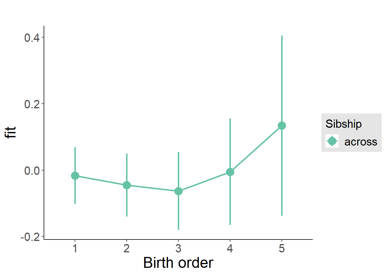
Add Interaction
Model Summary
m4_interaction = update(m3_birthorder_nonlinear, formula = . ~ . - birth_order_nonlinear - sibling_count + count_birth_order)
tidy(m4_interaction, conf.int = T, conf.level = 0.995)| effect | group | term | estimate | std.error | statistic | df | p.value | conf.low | conf.high |
|---|---|---|---|---|---|---|---|---|---|
| fixed | NA | (Intercept) | -1.203 | 0.5529 | -2.175 | 4475 | 0.02967 | -2.755 | 0.3494 |
| fixed | NA | poly(age, 3, raw = TRUE)1 | 0.09945 | 0.06455 | 1.541 | 4474 | 0.1235 | -0.08176 | 0.2807 |
| fixed | NA | poly(age, 3, raw = TRUE)2 | -0.002762 | 0.002382 | -1.159 | 4471 | 0.2463 | -0.00945 | 0.003925 |
| fixed | NA | poly(age, 3, raw = TRUE)3 | 0.00002825 | 0.00002797 | 1.01 | 4468 | 0.3126 | -0.00005027 | 0.0001068 |
| fixed | NA | male | 0.05823 | 0.02953 | 1.972 | 4426 | 0.04867 | -0.02466 | 0.1411 |
| fixed | NA | count_birth_order2/2 | -0.03221 | 0.05875 | -0.5482 | 3745 | 0.5836 | -0.1971 | 0.1327 |
| fixed | NA | count_birth_order1/3 | -0.03496 | 0.05246 | -0.6665 | 4467 | 0.5051 | -0.1822 | 0.1123 |
| fixed | NA | count_birth_order2/3 | -0.05099 | 0.05799 | -0.8793 | 4475 | 0.3793 | -0.2138 | 0.1118 |
| fixed | NA | count_birth_order3/3 | -0.1223 | 0.06371 | -1.919 | 4469 | 0.05505 | -0.3011 | 0.05657 |
| fixed | NA | count_birth_order1/4 | -0.088 | 0.06544 | -1.345 | 4473 | 0.1787 | -0.2717 | 0.09568 |
| fixed | NA | count_birth_order2/4 | -0.1098 | 0.06719 | -1.634 | 4474 | 0.1023 | -0.2984 | 0.0788 |
| fixed | NA | count_birth_order3/4 | -0.07642 | 0.07034 | -1.086 | 4461 | 0.2774 | -0.2739 | 0.121 |
| fixed | NA | count_birth_order4/4 | -0.01713 | 0.0743 | -0.2306 | 4456 | 0.8176 | -0.2257 | 0.1914 |
| fixed | NA | count_birth_order1/5 | 0.0415 | 0.0884 | 0.4695 | 4474 | 0.6388 | -0.2066 | 0.2896 |
| fixed | NA | count_birth_order2/5 | -0.02249 | 0.09749 | -0.2307 | 4455 | 0.8176 | -0.2962 | 0.2512 |
| fixed | NA | count_birth_order3/5 | -0.001968 | 0.0929 | -0.02118 | 4448 | 0.9831 | -0.2627 | 0.2588 |
| fixed | NA | count_birth_order4/5 | -0.02361 | 0.08947 | -0.264 | 4454 | 0.7918 | -0.2747 | 0.2275 |
| fixed | NA | count_birth_order5/5 | 0.1649 | 0.095 | 1.736 | 4443 | 0.0827 | -0.1018 | 0.4316 |
| ran_pars | mother_pidlink | sd__(Intercept) | 0.3058 | NA | NA | NA | NA | NA | NA |
| ran_pars | Residual | sd__Observation | 0.9426 | NA | NA | NA | NA | NA | NA |
Coefficient Plot
plot_birthorder(m4_interaction)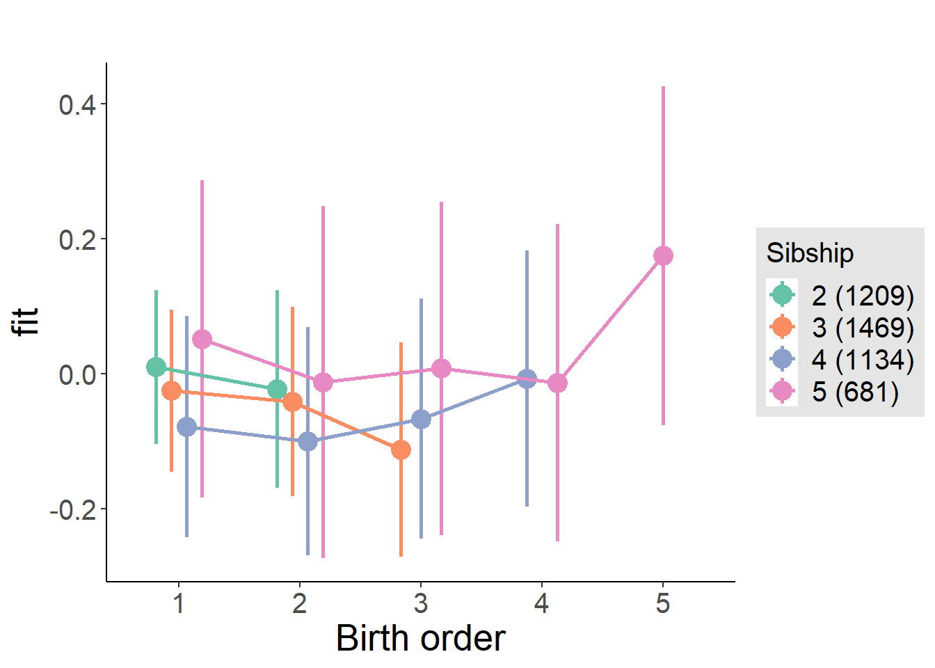
Model Comparison
###### Model 1 - Model 2
anova(m1_covariates_only, m2_birthorder_linear, m3_birthorder_nonlinear, m4_interaction)## refitting model(s) with ML (instead of REML)| Df | AIC | BIC | logLik | deviance | Chisq | Chi Df | Pr(>Chisq) |
|---|---|---|---|---|---|---|---|
| 10 | 12662 | 12726 | -6321 | 12642 | NA | NA | NA |
| 11 | 12664 | 12734 | -6321 | 12642 | 0.03329 | 1 | 0.8552 |
| 14 | 12665 | 12755 | -6319 | 12637 | 4.585 | 3 | 0.2048 |
| 20 | 12675 | 12803 | -6318 | 12635 | 2.189 | 6 | 0.9015 |
Compare birth order specifications
library(coefplot)
multiplot(outcome_naive_m1, outcome_preg_m1, outcome_uterus_m1, outcome_parental_m1, dodgeHeight = 0.6,
intercept = FALSE)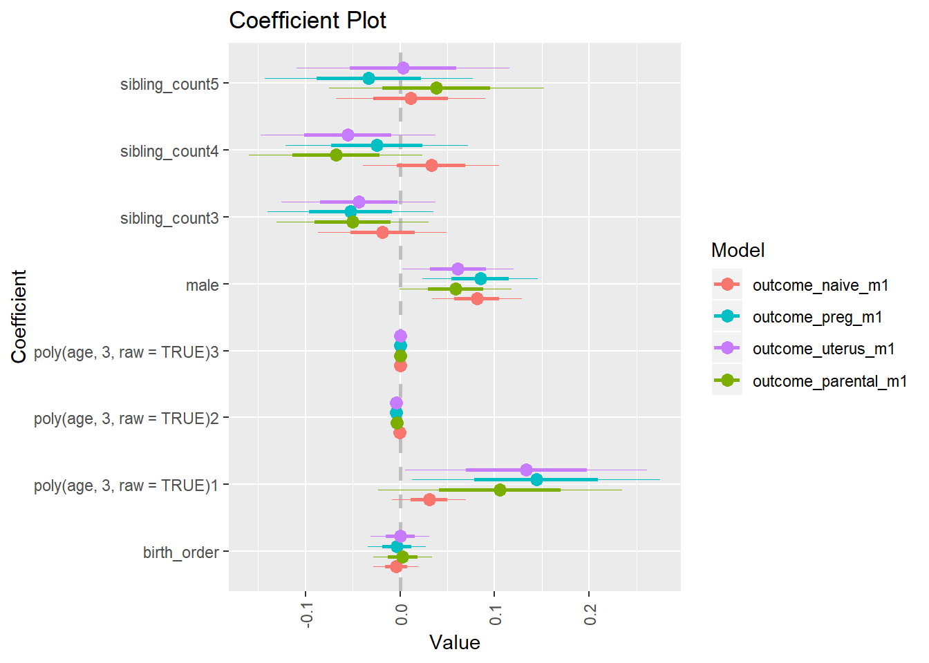
Openness
birthorder <- birthorder %>% mutate(outcome = big5_open)
model = lmer(outcome ~ birth_order + poly(age, 3, raw = TRUE) + male + sibling_count + (1 | mother_pidlink),
data = birthorder)
compare_birthorder_specs(model)Naive birth order
outcome_naive_m1 <- update(m2_birthorder_linear, data = birthorder %>%
mutate(sibling_count = sibling_count_naive_factor,
birth_order_nonlinear = birthorder_naive_factor,
birth_order = birthorder_naive,
count_birth_order = count_birthorder_naive) %>%
filter(sibling_count != "1"))
compare_models_markdown(outcome_naive_m1)Basic Model
Model Summary
m1_covariates_only <- update(m2_birthorder_linear, formula = . ~ . - birth_order)
tidy(m1_covariates_only, conf.int = T, conf.level = 0.995)| effect | group | term | estimate | std.error | statistic | df | p.value | conf.low | conf.high |
|---|---|---|---|---|---|---|---|---|---|
| fixed | NA | (Intercept) | 0.1884 | 0.1972 | 0.9556 | 6706 | 0.3393 | -0.3651 | 0.7419 |
| fixed | NA | poly(age, 3, raw = TRUE)1 | -0.01562 | 0.01894 | -0.8246 | 6526 | 0.4097 | -0.06878 | 0.03754 |
| fixed | NA | poly(age, 3, raw = TRUE)2 | 0.0004604 | 0.000553 | 0.8325 | 6323 | 0.4051 | -0.001092 | 0.002013 |
| fixed | NA | poly(age, 3, raw = TRUE)3 | -0.000005537 | 0.000005017 | -1.104 | 6167 | 0.2697 | -0.00001962 | 0.000008545 |
| fixed | NA | male | 0.1661 | 0.023 | 7.222 | 7062 | 5.643e-13 | 0.1016 | 0.2307 |
| fixed | NA | sibling_count3 | -0.02065 | 0.03284 | -0.6287 | 4991 | 0.5296 | -0.1128 | 0.07154 |
| fixed | NA | sibling_count4 | -0.05262 | 0.03382 | -1.556 | 4419 | 0.1199 | -0.1476 | 0.04233 |
| fixed | NA | sibling_count5 | -0.01423 | 0.03514 | -0.4048 | 3819 | 0.6856 | -0.1129 | 0.08442 |
| ran_pars | mother_pidlink | sd__(Intercept) | 0.2814 | NA | NA | NA | NA | NA | NA |
| ran_pars | Residual | sd__Observation | 0.9325 | NA | NA | NA | NA | NA | NA |
Coefficient Plot
plot(allEffects(m1_covariates_only, confidence.level = 0.995))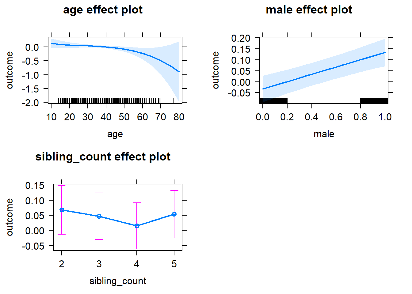
Add Birth Order Linear
Model Summary
tidy(m2_birthorder_linear, conf.int = T, conf.level = 0.995)| effect | group | term | estimate | std.error | statistic | df | p.value | conf.low | conf.high |
|---|---|---|---|---|---|---|---|---|---|
| fixed | NA | (Intercept) | 0.1939 | 0.1972 | 0.983 | 6695 | 0.3257 | -0.3598 | 0.7475 |
| fixed | NA | birth_order | -0.0152 | 0.0115 | -1.322 | 6118 | 0.1862 | -0.04749 | 0.01708 |
| fixed | NA | poly(age, 3, raw = TRUE)1 | -0.0141 | 0.01897 | -0.7432 | 6554 | 0.4574 | -0.06736 | 0.03916 |
| fixed | NA | poly(age, 3, raw = TRUE)2 | 0.0004218 | 0.0005538 | 0.7617 | 6339 | 0.4463 | -0.001133 | 0.001976 |
| fixed | NA | poly(age, 3, raw = TRUE)3 | -0.000005287 | 0.000005021 | -1.053 | 6176 | 0.2924 | -0.00001938 | 0.000008806 |
| fixed | NA | male | 0.1666 | 0.023 | 7.242 | 7060 | 4.905e-13 | 0.102 | 0.2311 |
| fixed | NA | sibling_count3 | -0.01521 | 0.0331 | -0.4594 | 5121 | 0.646 | -0.1081 | 0.07771 |
| fixed | NA | sibling_count4 | -0.03998 | 0.03516 | -1.137 | 4975 | 0.2555 | -0.1387 | 0.0587 |
| fixed | NA | sibling_count5 | 0.006125 | 0.03837 | 0.1596 | 4933 | 0.8732 | -0.1016 | 0.1138 |
| ran_pars | mother_pidlink | sd__(Intercept) | 0.2824 | NA | NA | NA | NA | NA | NA |
| ran_pars | Residual | sd__Observation | 0.9322 | NA | NA | NA | NA | NA | NA |
Coefficient Plot
plot_birthorder2(m2_birthorder_linear, separate = FALSE)
Add Birth Order Factor
Model Summary
m3_birthorder_nonlinear = update(m1_covariates_only, formula = . ~ . + birth_order_nonlinear)
tidy(m3_birthorder_nonlinear, conf.int = T, conf.level = 0.995)| effect | group | term | estimate | std.error | statistic | df | p.value | conf.low | conf.high |
|---|---|---|---|---|---|---|---|---|---|
| fixed | NA | (Intercept) | 0.1783 | 0.1978 | 0.9016 | 6719 | 0.3673 | -0.3768 | 0.7335 |
| fixed | NA | poly(age, 3, raw = TRUE)1 | -0.01421 | 0.01898 | -0.7484 | 6540 | 0.4543 | -0.06749 | 0.03908 |
| fixed | NA | poly(age, 3, raw = TRUE)2 | 0.0004305 | 0.0005542 | 0.7768 | 6315 | 0.4373 | -0.001125 | 0.001986 |
| fixed | NA | poly(age, 3, raw = TRUE)3 | -0.000005414 | 0.000005026 | -1.077 | 6140 | 0.2814 | -0.00001952 | 0.000008694 |
| fixed | NA | male | 0.1666 | 0.023 | 7.245 | 7057 | 4.794e-13 | 0.1021 | 0.2312 |
| fixed | NA | sibling_count3 | -0.004773 | 0.03363 | -0.1419 | 5340 | 0.8871 | -0.09917 | 0.08963 |
| fixed | NA | sibling_count4 | -0.03468 | 0.03574 | -0.9704 | 5223 | 0.3319 | -0.135 | 0.06565 |
| fixed | NA | sibling_count5 | 0.005849 | 0.03875 | 0.151 | 5113 | 0.88 | -0.1029 | 0.1146 |
| fixed | NA | birth_order_nonlinear2 | -0.01603 | 0.02733 | -0.5864 | 5985 | 0.5577 | -0.09276 | 0.0607 |
| fixed | NA | birth_order_nonlinear3 | -0.0772 | 0.03508 | -2.201 | 5947 | 0.0278 | -0.1757 | 0.02128 |
| fixed | NA | birth_order_nonlinear4 | -0.02083 | 0.04582 | -0.4546 | 5958 | 0.6494 | -0.1494 | 0.1078 |
| fixed | NA | birth_order_nonlinear5 | -0.02959 | 0.06668 | -0.4438 | 5840 | 0.6572 | -0.2168 | 0.1576 |
| ran_pars | mother_pidlink | sd__(Intercept) | 0.2822 | NA | NA | NA | NA | NA | NA |
| ran_pars | Residual | sd__Observation | 0.9322 | NA | NA | NA | NA | NA | NA |
Coefficient Plot
plot_birthorder(m3_birthorder_nonlinear, separate = FALSE)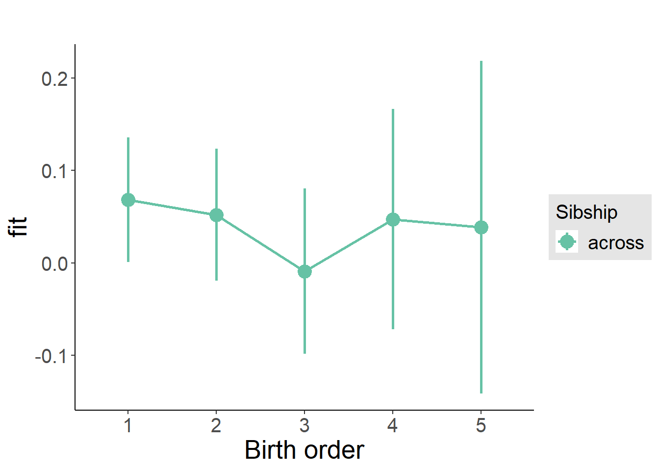
Add Interaction
Model Summary
m4_interaction = update(m3_birthorder_nonlinear, formula = . ~ . - birth_order_nonlinear - sibling_count + count_birth_order)
tidy(m4_interaction, conf.int = T, conf.level = 0.995)| effect | group | term | estimate | std.error | statistic | df | p.value | conf.low | conf.high |
|---|---|---|---|---|---|---|---|---|---|
| fixed | NA | (Intercept) | 0.201 | 0.1981 | 1.015 | 6724 | 0.3103 | -0.3551 | 0.7572 |
| fixed | NA | poly(age, 3, raw = TRUE)1 | -0.0141 | 0.01898 | -0.7431 | 6537 | 0.4574 | -0.06738 | 0.03917 |
| fixed | NA | poly(age, 3, raw = TRUE)2 | 0.0004332 | 0.0005541 | 0.7818 | 6309 | 0.4344 | -0.001122 | 0.001988 |
| fixed | NA | poly(age, 3, raw = TRUE)3 | -0.000005479 | 0.000005025 | -1.09 | 6130 | 0.2756 | -0.00001958 | 0.000008626 |
| fixed | NA | male | 0.1664 | 0.023 | 7.233 | 7051 | 5.225e-13 | 0.1018 | 0.231 |
| fixed | NA | count_birth_order2/2 | -0.08506 | 0.04665 | -1.824 | 5931 | 0.06828 | -0.216 | 0.04588 |
| fixed | NA | count_birth_order1/3 | -0.05985 | 0.04394 | -1.362 | 7113 | 0.1732 | -0.1832 | 0.06349 |
| fixed | NA | count_birth_order2/3 | -0.02781 | 0.04914 | -0.5659 | 7125 | 0.5714 | -0.1658 | 0.1101 |
| fixed | NA | count_birth_order3/3 | -0.07335 | 0.0551 | -1.331 | 7128 | 0.1832 | -0.228 | 0.08133 |
| fixed | NA | count_birth_order1/4 | -0.07601 | 0.0502 | -1.514 | 7126 | 0.1301 | -0.2169 | 0.06491 |
| fixed | NA | count_birth_order2/4 | -0.01537 | 0.0528 | -0.291 | 7128 | 0.7711 | -0.1636 | 0.1329 |
| fixed | NA | count_birth_order3/4 | -0.1879 | 0.0574 | -3.273 | 7128 | 0.00107 | -0.349 | -0.02673 |
| fixed | NA | count_birth_order4/4 | -0.08668 | 0.06082 | -1.425 | 7124 | 0.1542 | -0.2574 | 0.08405 |
| fixed | NA | count_birth_order1/5 | -0.005622 | 0.05698 | -0.09866 | 7128 | 0.9214 | -0.1656 | 0.1543 |
| fixed | NA | count_birth_order2/5 | -0.07134 | 0.05996 | -1.19 | 7124 | 0.2342 | -0.2397 | 0.09698 |
| fixed | NA | count_birth_order3/5 | -0.08237 | 0.06156 | -1.338 | 7121 | 0.1809 | -0.2552 | 0.09043 |
| fixed | NA | count_birth_order4/5 | -0.03452 | 0.06525 | -0.5291 | 7115 | 0.5967 | -0.2177 | 0.1486 |
| fixed | NA | count_birth_order5/5 | -0.04936 | 0.06671 | -0.74 | 7111 | 0.4593 | -0.2366 | 0.1379 |
| ran_pars | mother_pidlink | sd__(Intercept) | 0.2805 | NA | NA | NA | NA | NA | NA |
| ran_pars | Residual | sd__Observation | 0.9326 | NA | NA | NA | NA | NA | NA |
Coefficient Plot
plot_birthorder(m4_interaction)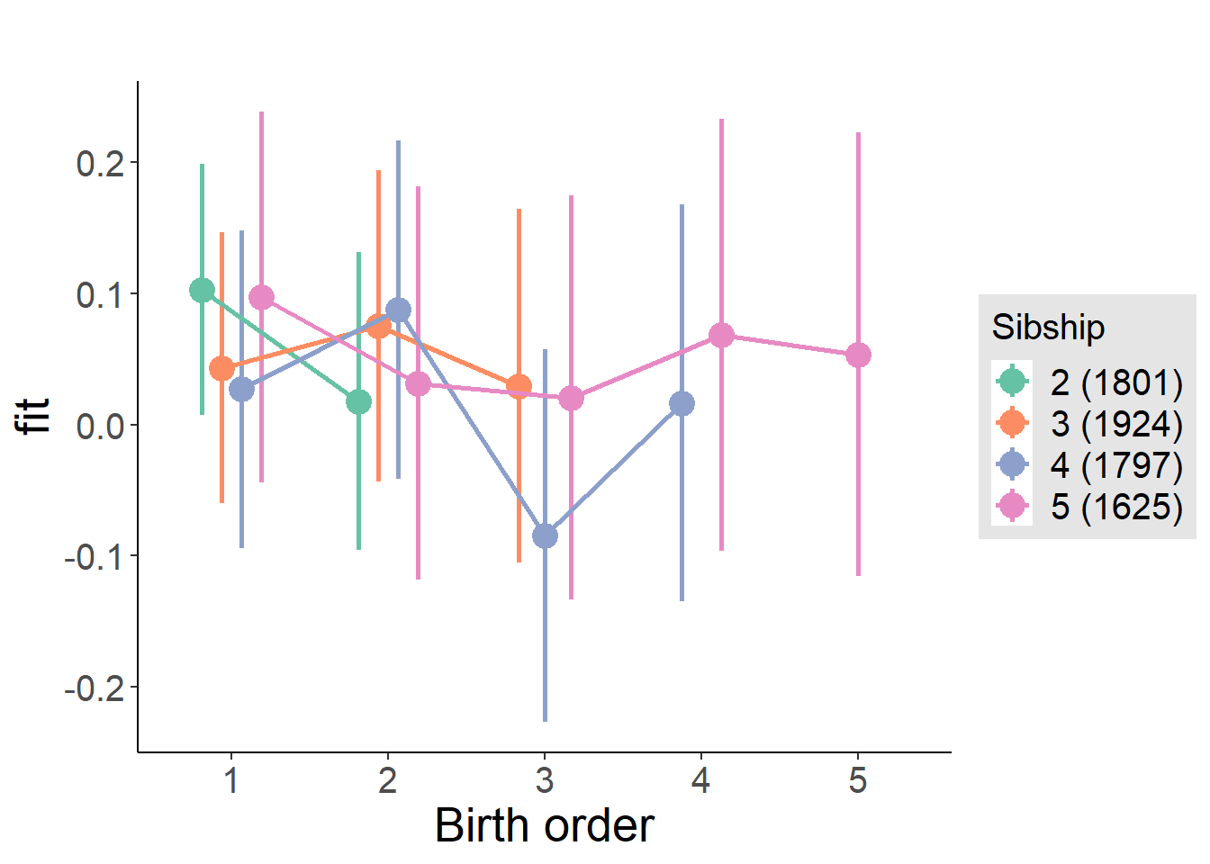
Model Comparison
###### Model 1 - Model 2
anova(m1_covariates_only, m2_birthorder_linear, m3_birthorder_nonlinear, m4_interaction)## refitting model(s) with ML (instead of REML)| Df | AIC | BIC | logLik | deviance | Chisq | Chi Df | Pr(>Chisq) |
|---|---|---|---|---|---|---|---|
| 10 | 19896 | 19965 | -9938 | 19876 | NA | NA | NA |
| 11 | 19896 | 19972 | -9937 | 19874 | 1.746 | 1 | 0.1864 |
| 14 | 19899 | 19995 | -9936 | 19871 | 3.169 | 3 | 0.3663 |
| 20 | 19903 | 20041 | -9932 | 19863 | 7.754 | 6 | 0.2567 |
Maternal birth order
outcome_uterus_m1 <- update(m2_birthorder_linear, data = birthorder %>%
mutate(sibling_count = sibling_count_uterus_alive_factor,
birth_order_nonlinear = birthorder_uterus_alive_factor,
birth_order = birthorder_uterus_alive,
count_birth_order = count_birthorder_uterus_alive) %>%
filter(sibling_count != "1"))
compare_models_markdown(outcome_uterus_m1)Basic Model
Model Summary
m1_covariates_only <- update(m2_birthorder_linear, formula = . ~ . - birth_order)
tidy(m1_covariates_only, conf.int = T, conf.level = 0.995)| effect | group | term | estimate | std.error | statistic | df | p.value | conf.low | conf.high |
|---|---|---|---|---|---|---|---|---|---|
| fixed | NA | (Intercept) | -1.131 | 0.5097 | -2.218 | 4499 | 0.02658 | -2.561 | 0.3 |
| fixed | NA | poly(age, 3, raw = TRUE)1 | 0.1491 | 0.05948 | 2.507 | 4500 | 0.01222 | -0.01785 | 0.3161 |
| fixed | NA | poly(age, 3, raw = TRUE)2 | -0.00554 | 0.002192 | -2.528 | 4498 | 0.01152 | -0.01169 | 0.0006123 |
| fixed | NA | poly(age, 3, raw = TRUE)3 | 0.00006508 | 0.00002568 | 2.535 | 4496 | 0.01129 | -0.000006995 | 0.0001372 |
| fixed | NA | male | 0.1181 | 0.02745 | 4.304 | 4448 | 0.00001717 | 0.04108 | 0.1952 |
| fixed | NA | sibling_count3 | -0.09546 | 0.03738 | -2.553 | 3304 | 0.01071 | -0.2004 | 0.009483 |
| fixed | NA | sibling_count4 | -0.0851 | 0.04034 | -2.11 | 2863 | 0.03496 | -0.1983 | 0.02812 |
| fixed | NA | sibling_count5 | -0.1082 | 0.04601 | -2.352 | 2517 | 0.01874 | -0.2374 | 0.02092 |
| ran_pars | mother_pidlink | sd__(Intercept) | 0.2964 | NA | NA | NA | NA | NA | NA |
| ran_pars | Residual | sd__Observation | 0.8755 | NA | NA | NA | NA | NA | NA |
Coefficient Plot
plot(allEffects(m1_covariates_only, confidence.level = 0.995))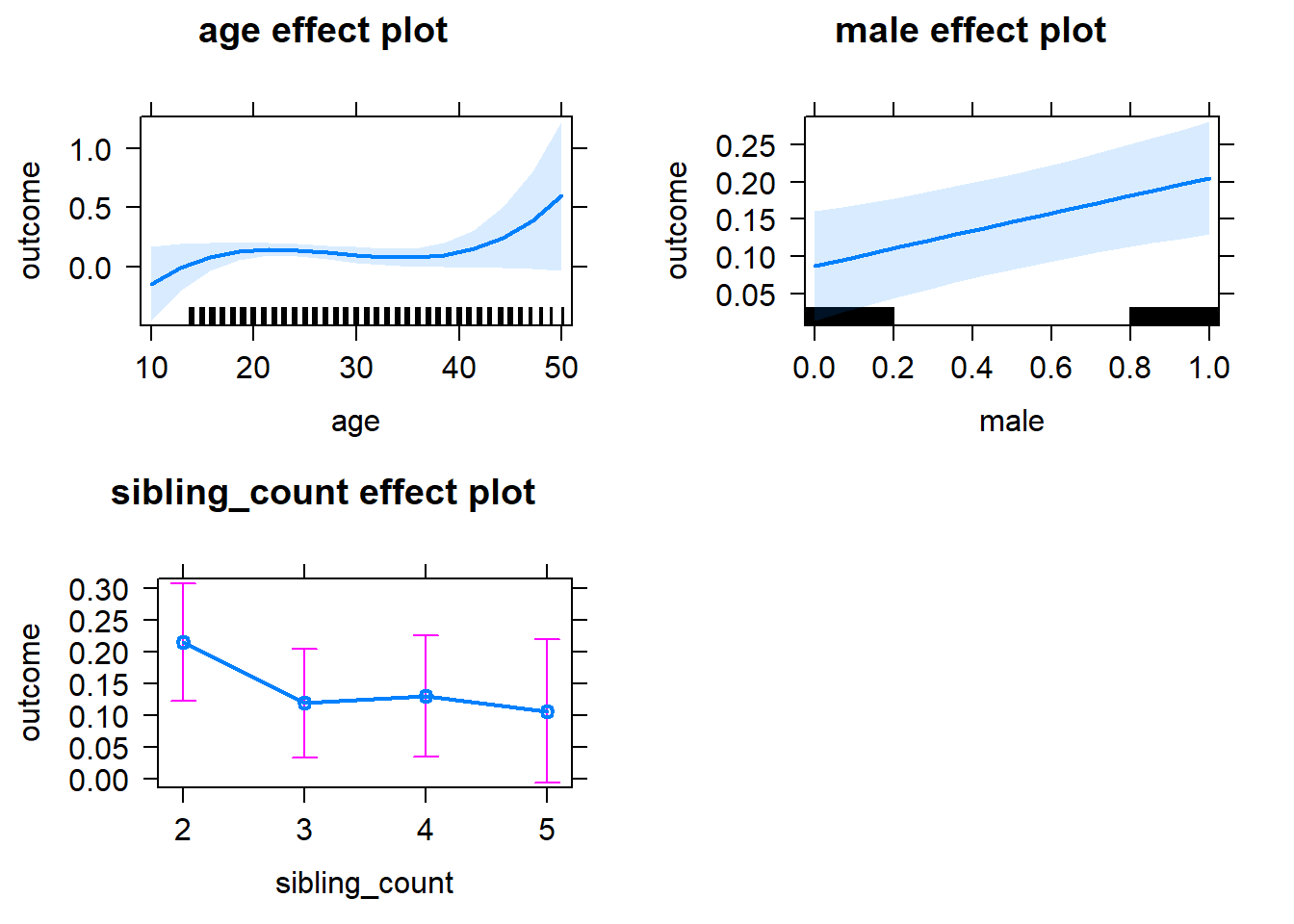
Add Birth Order Linear
Model Summary
tidy(m2_birthorder_linear, conf.int = T, conf.level = 0.995)| effect | group | term | estimate | std.error | statistic | df | p.value | conf.low | conf.high |
|---|---|---|---|---|---|---|---|---|---|
| fixed | NA | (Intercept) | -1.157 | 0.5102 | -2.268 | 4499 | 0.02337 | -2.589 | 0.275 |
| fixed | NA | birth_order | 0.01578 | 0.01441 | 1.095 | 4179 | 0.2737 | -0.02468 | 0.05624 |
| fixed | NA | poly(age, 3, raw = TRUE)1 | 0.15 | 0.05948 | 2.522 | 4499 | 0.01169 | -0.01693 | 0.317 |
| fixed | NA | poly(age, 3, raw = TRUE)2 | -0.005592 | 0.002192 | -2.551 | 4498 | 0.01078 | -0.01175 | 0.0005614 |
| fixed | NA | poly(age, 3, raw = TRUE)3 | 0.00006602 | 0.00002569 | 2.57 | 4495 | 0.01021 | -0.000006098 | 0.0001381 |
| fixed | NA | male | 0.1176 | 0.02745 | 4.284 | 4447 | 0.00001873 | 0.04055 | 0.1947 |
| fixed | NA | sibling_count3 | -0.1027 | 0.03796 | -2.706 | 3367 | 0.006852 | -0.2092 | 0.003849 |
| fixed | NA | sibling_count4 | -0.1018 | 0.0431 | -2.361 | 3098 | 0.01828 | -0.2227 | 0.01922 |
| fixed | NA | sibling_count5 | -0.1361 | 0.05256 | -2.589 | 3046 | 0.00967 | -0.2836 | 0.01146 |
| ran_pars | mother_pidlink | sd__(Intercept) | 0.2957 | NA | NA | NA | NA | NA | NA |
| ran_pars | Residual | sd__Observation | 0.8757 | NA | NA | NA | NA | NA | NA |
Coefficient Plot
plot_birthorder2(m2_birthorder_linear, separate = FALSE)
Add Birth Order Factor
Model Summary
m3_birthorder_nonlinear = update(m1_covariates_only, formula = . ~ . + birth_order_nonlinear)
tidy(m3_birthorder_nonlinear, conf.int = T, conf.level = 0.995)| effect | group | term | estimate | std.error | statistic | df | p.value | conf.low | conf.high |
|---|---|---|---|---|---|---|---|---|---|
| fixed | NA | (Intercept) | -1.124 | 0.5107 | -2.201 | 4496 | 0.02779 | -2.558 | 0.3096 |
| fixed | NA | poly(age, 3, raw = TRUE)1 | 0.148 | 0.05955 | 2.486 | 4495 | 0.01296 | -0.01912 | 0.3152 |
| fixed | NA | poly(age, 3, raw = TRUE)2 | -0.005521 | 0.002195 | -2.516 | 4493 | 0.01191 | -0.01168 | 0.0006393 |
| fixed | NA | poly(age, 3, raw = TRUE)3 | 0.00006527 | 0.00002572 | 2.538 | 4491 | 0.01118 | -0.000006915 | 0.0001375 |
| fixed | NA | male | 0.1174 | 0.02746 | 4.274 | 4443 | 0.00001961 | 0.04028 | 0.1945 |
| fixed | NA | sibling_count3 | -0.09381 | 0.03857 | -2.432 | 3488 | 0.01505 | -0.2021 | 0.01445 |
| fixed | NA | sibling_count4 | -0.09743 | 0.04376 | -2.226 | 3200 | 0.02606 | -0.2203 | 0.02541 |
| fixed | NA | sibling_count5 | -0.1417 | 0.05348 | -2.65 | 3136 | 0.008091 | -0.2918 | 0.008401 |
| fixed | NA | birth_order_nonlinear2 | 0.01459 | 0.03273 | 0.4457 | 3623 | 0.6558 | -0.07728 | 0.1064 |
| fixed | NA | birth_order_nonlinear3 | -0.007921 | 0.04171 | -0.1899 | 3848 | 0.8494 | -0.125 | 0.1092 |
| fixed | NA | birth_order_nonlinear4 | 0.06769 | 0.056 | 1.209 | 4040 | 0.2268 | -0.0895 | 0.2249 |
| fixed | NA | birth_order_nonlinear5 | 0.1049 | 0.0872 | 1.203 | 3908 | 0.229 | -0.1399 | 0.3497 |
| ran_pars | mother_pidlink | sd__(Intercept) | 0.2965 | NA | NA | NA | NA | NA | NA |
| ran_pars | Residual | sd__Observation | 0.8756 | NA | NA | NA | NA | NA | NA |
Coefficient Plot
plot_birthorder(m3_birthorder_nonlinear, separate = FALSE)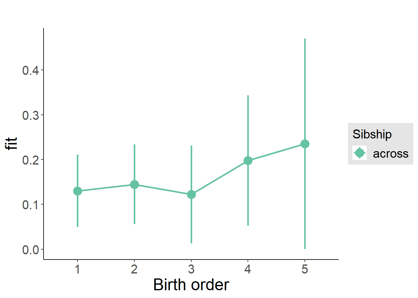
Add Interaction
Model Summary
m4_interaction = update(m3_birthorder_nonlinear, formula = . ~ . - birth_order_nonlinear - sibling_count + count_birth_order)
tidy(m4_interaction, conf.int = T, conf.level = 0.995)| effect | group | term | estimate | std.error | statistic | df | p.value | conf.low | conf.high |
|---|---|---|---|---|---|---|---|---|---|
| fixed | NA | (Intercept) | -1.119 | 0.5109 | -2.19 | 4490 | 0.02855 | -2.553 | 0.3151 |
| fixed | NA | poly(age, 3, raw = TRUE)1 | 0.1483 | 0.05957 | 2.489 | 4490 | 0.01285 | -0.01895 | 0.3155 |
| fixed | NA | poly(age, 3, raw = TRUE)2 | -0.005511 | 0.002196 | -2.51 | 4488 | 0.01211 | -0.01167 | 0.0006524 |
| fixed | NA | poly(age, 3, raw = TRUE)3 | 0.00006492 | 0.00002573 | 2.523 | 4485 | 0.01167 | -0.00000731 | 0.0001372 |
| fixed | NA | male | 0.1182 | 0.02748 | 4.301 | 4436 | 0.00001739 | 0.04105 | 0.1953 |
| fixed | NA | count_birth_order2/2 | -0.01883 | 0.05617 | -0.3353 | 3805 | 0.7374 | -0.1765 | 0.1388 |
| fixed | NA | count_birth_order1/3 | -0.1352 | 0.04953 | -2.73 | 4482 | 0.006358 | -0.2742 | 0.003814 |
| fixed | NA | count_birth_order2/3 | -0.07522 | 0.0541 | -1.39 | 4490 | 0.1645 | -0.2271 | 0.07665 |
| fixed | NA | count_birth_order3/3 | -0.07505 | 0.06047 | -1.241 | 4486 | 0.2146 | -0.2448 | 0.0947 |
| fixed | NA | count_birth_order1/4 | -0.07112 | 0.06076 | -1.171 | 4487 | 0.2418 | -0.2417 | 0.09943 |
| fixed | NA | count_birth_order2/4 | -0.1272 | 0.06278 | -2.025 | 4489 | 0.04288 | -0.3034 | 0.04907 |
| fixed | NA | count_birth_order3/4 | -0.1429 | 0.06629 | -2.155 | 4477 | 0.03119 | -0.3289 | 0.0432 |
| fixed | NA | count_birth_order4/4 | -0.024 | 0.06885 | -0.3485 | 4475 | 0.7275 | -0.2173 | 0.1693 |
| fixed | NA | count_birth_order1/5 | -0.1653 | 0.08263 | -2 | 4487 | 0.04552 | -0.3972 | 0.06666 |
| fixed | NA | count_birth_order2/5 | -0.04699 | 0.08822 | -0.5327 | 4469 | 0.5943 | -0.2946 | 0.2006 |
| fixed | NA | count_birth_order3/5 | -0.1978 | 0.08265 | -2.394 | 4464 | 0.01671 | -0.4298 | 0.03415 |
| fixed | NA | count_birth_order4/5 | -0.1109 | 0.07957 | -1.394 | 4470 | 0.1634 | -0.3343 | 0.1124 |
| fixed | NA | count_birth_order5/5 | -0.04873 | 0.08275 | -0.5889 | 4457 | 0.556 | -0.281 | 0.1836 |
| ran_pars | mother_pidlink | sd__(Intercept) | 0.2966 | NA | NA | NA | NA | NA | NA |
| ran_pars | Residual | sd__Observation | 0.8757 | NA | NA | NA | NA | NA | NA |
Coefficient Plot
plot_birthorder(m4_interaction)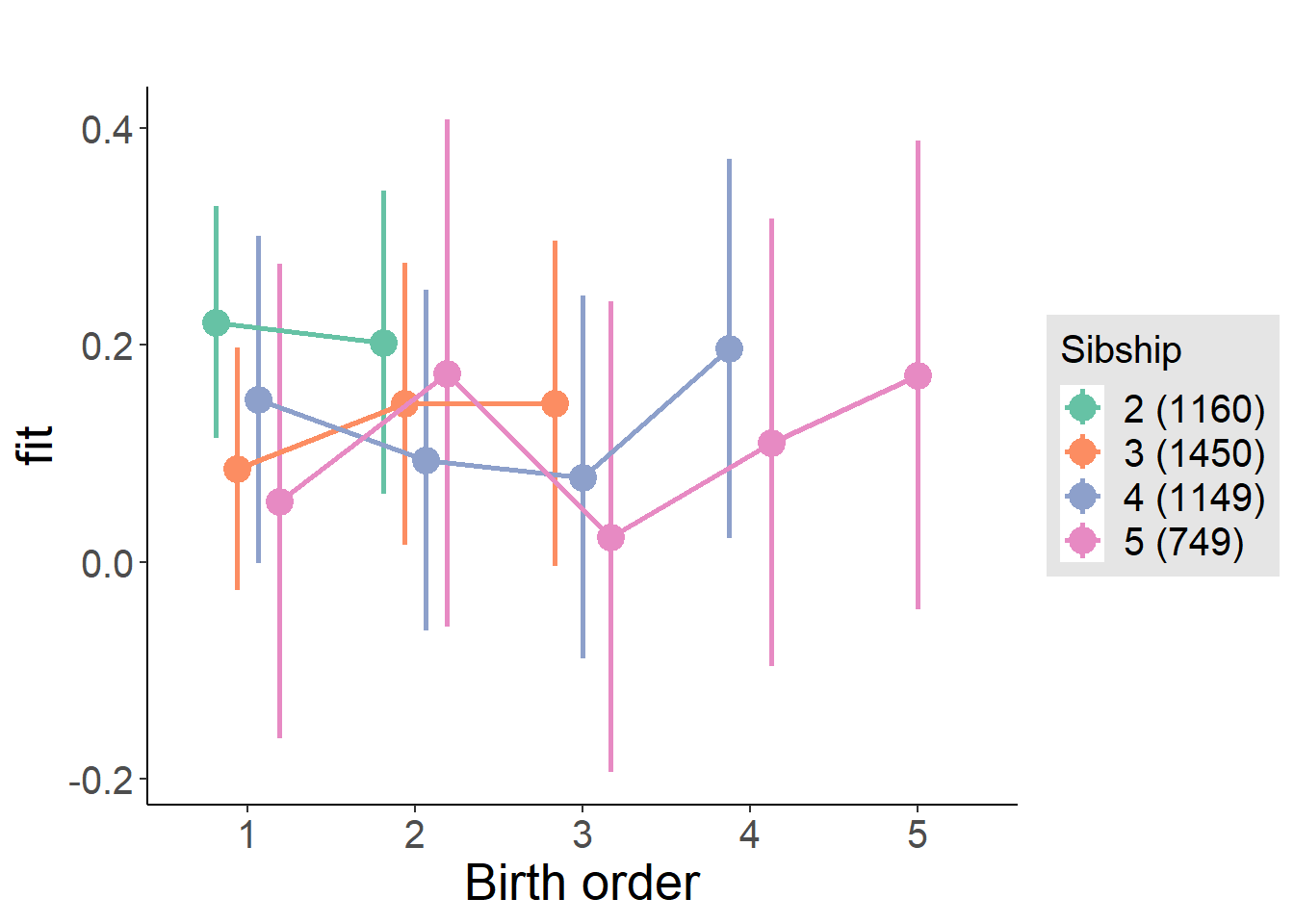
Model Comparison
###### Model 1 - Model 2
anova(m1_covariates_only, m2_birthorder_linear, m3_birthorder_nonlinear, m4_interaction)## refitting model(s) with ML (instead of REML)| Df | AIC | BIC | logLik | deviance | Chisq | Chi Df | Pr(>Chisq) |
|---|---|---|---|---|---|---|---|
| 10 | 12078 | 12142 | -6029 | 12058 | NA | NA | NA |
| 11 | 12078 | 12149 | -6028 | 12056 | 1.202 | 1 | 0.273 |
| 14 | 12083 | 12172 | -6027 | 12055 | 1.724 | 3 | 0.6316 |
| 20 | 12090 | 12218 | -6025 | 12050 | 4.844 | 6 | 0.5639 |
Maternal pregnancy order
outcome_preg_m1 <- update(m2_birthorder_linear, data = birthorder %>%
mutate(sibling_count = sibling_count_uterus_preg_factor,
birth_order_nonlinear = birthorder_uterus_preg_factor,
birth_order = birthorder_uterus_preg,
count_birth_order = count_birthorder_uterus_preg
) %>%
filter(sibling_count != "1"))
compare_models_markdown(outcome_preg_m1)Basic Model
Model Summary
m1_covariates_only <- update(m2_birthorder_linear, formula = . ~ . - birth_order)
tidy(m1_covariates_only, conf.int = T, conf.level = 0.995)| effect | group | term | estimate | std.error | statistic | df | p.value | conf.low | conf.high |
|---|---|---|---|---|---|---|---|---|---|
| fixed | NA | (Intercept) | -1.319 | 0.5255 | -2.509 | 4175 | 0.01214 | -2.794 | 0.1566 |
| fixed | NA | poly(age, 3, raw = TRUE)1 | 0.1718 | 0.06139 | 2.798 | 4177 | 0.005168 | -0.0005629 | 0.3441 |
| fixed | NA | poly(age, 3, raw = TRUE)2 | -0.006328 | 0.002263 | -2.796 | 4177 | 0.005196 | -0.01268 | 0.00002468 |
| fixed | NA | poly(age, 3, raw = TRUE)3 | 0.00007372 | 0.00002652 | 2.78 | 4175 | 0.005459 | -0.0000007143 | 0.0001482 |
| fixed | NA | male | 0.118 | 0.02852 | 4.139 | 4114 | 0.00003561 | 0.03798 | 0.1981 |
| fixed | NA | sibling_count3 | -0.1239 | 0.0406 | -3.052 | 3147 | 0.002291 | -0.2379 | -0.009953 |
| fixed | NA | sibling_count4 | -0.09755 | 0.04293 | -2.272 | 2846 | 0.02316 | -0.2181 | 0.02297 |
| fixed | NA | sibling_count5 | -0.1168 | 0.04598 | -2.541 | 2527 | 0.01112 | -0.2459 | 0.01224 |
| ran_pars | mother_pidlink | sd__(Intercept) | 0.3139 | NA | NA | NA | NA | NA | NA |
| ran_pars | Residual | sd__Observation | 0.871 | NA | NA | NA | NA | NA | NA |
Coefficient Plot
plot(allEffects(m1_covariates_only, confidence.level = 0.995))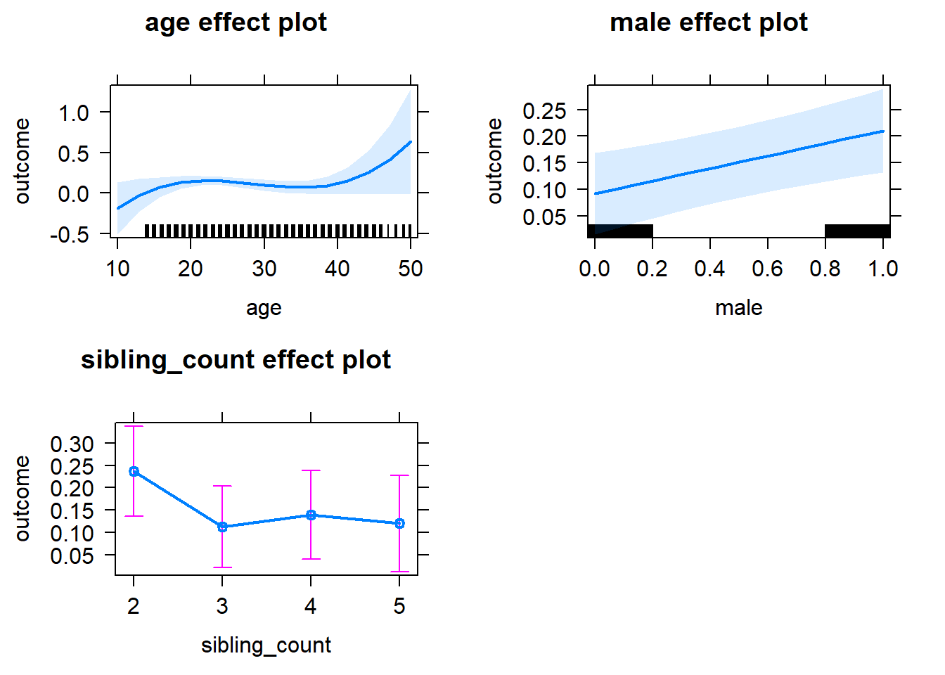
Add Birth Order Linear
Model Summary
tidy(m2_birthorder_linear, conf.int = T, conf.level = 0.995)| effect | group | term | estimate | std.error | statistic | df | p.value | conf.low | conf.high |
|---|---|---|---|---|---|---|---|---|---|
| fixed | NA | (Intercept) | -1.356 | 0.526 | -2.578 | 4174 | 0.00998 | -2.832 | 0.1206 |
| fixed | NA | birth_order | 0.02246 | 0.01444 | 1.555 | 3942 | 0.1201 | -0.01809 | 0.063 |
| fixed | NA | poly(age, 3, raw = TRUE)1 | 0.1729 | 0.06138 | 2.817 | 4176 | 0.00487 | 0.0006121 | 0.3452 |
| fixed | NA | poly(age, 3, raw = TRUE)2 | -0.006394 | 0.002263 | -2.825 | 4176 | 0.004747 | -0.01275 | -0.00004116 |
| fixed | NA | poly(age, 3, raw = TRUE)3 | 0.00007495 | 0.00002653 | 2.826 | 4175 | 0.004742 | 0.0000004923 | 0.0001494 |
| fixed | NA | male | 0.1176 | 0.02852 | 4.122 | 4113 | 0.00003828 | 0.0375 | 0.1976 |
| fixed | NA | sibling_count3 | -0.1342 | 0.04113 | -3.263 | 3191 | 0.001113 | -0.2496 | -0.01876 |
| fixed | NA | sibling_count4 | -0.1205 | 0.04538 | -2.654 | 3016 | 0.007985 | -0.2479 | 0.006923 |
| fixed | NA | sibling_count5 | -0.1534 | 0.05165 | -2.971 | 2929 | 0.002994 | -0.2984 | -0.008461 |
| ran_pars | mother_pidlink | sd__(Intercept) | 0.3134 | NA | NA | NA | NA | NA | NA |
| ran_pars | Residual | sd__Observation | 0.871 | NA | NA | NA | NA | NA | NA |
Coefficient Plot
plot_birthorder2(m2_birthorder_linear, separate = FALSE)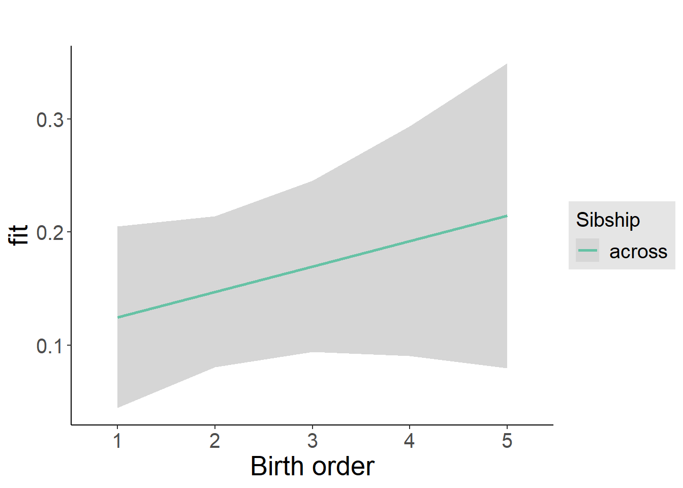
Add Birth Order Factor
Model Summary
m3_birthorder_nonlinear = update(m1_covariates_only, formula = . ~ . + birth_order_nonlinear)
tidy(m3_birthorder_nonlinear, conf.int = T, conf.level = 0.995)| effect | group | term | estimate | std.error | statistic | df | p.value | conf.low | conf.high |
|---|---|---|---|---|---|---|---|---|---|
| fixed | NA | (Intercept) | -1.303 | 0.5263 | -2.476 | 4173 | 0.01331 | -2.78 | 0.174 |
| fixed | NA | poly(age, 3, raw = TRUE)1 | 0.17 | 0.06142 | 2.767 | 4173 | 0.005678 | -0.002444 | 0.3424 |
| fixed | NA | poly(age, 3, raw = TRUE)2 | -0.00629 | 0.002264 | -2.778 | 4172 | 0.005499 | -0.01265 | 0.00006647 |
| fixed | NA | poly(age, 3, raw = TRUE)3 | 0.00007387 | 0.00002654 | 2.784 | 4171 | 0.005402 | -0.0000006244 | 0.0001484 |
| fixed | NA | male | 0.117 | 0.02851 | 4.104 | 4108 | 0.00004133 | 0.03699 | 0.1971 |
| fixed | NA | sibling_count3 | -0.1232 | 0.04174 | -2.952 | 3291 | 0.003177 | -0.2404 | -0.00606 |
| fixed | NA | sibling_count4 | -0.1266 | 0.04603 | -2.75 | 3108 | 0.005997 | -0.2558 | 0.002632 |
| fixed | NA | sibling_count5 | -0.153 | 0.0522 | -2.931 | 2981 | 0.003409 | -0.2995 | -0.006448 |
| fixed | NA | birth_order_nonlinear2 | 0.008347 | 0.034 | 0.2455 | 3400 | 0.8061 | -0.08709 | 0.1038 |
| fixed | NA | birth_order_nonlinear3 | -0.005034 | 0.04301 | -0.117 | 3618 | 0.9068 | -0.1258 | 0.1157 |
| fixed | NA | birth_order_nonlinear4 | 0.1464 | 0.05694 | 2.571 | 3773 | 0.01018 | -0.01344 | 0.3062 |
| fixed | NA | birth_order_nonlinear5 | 0.04786 | 0.08343 | 0.5736 | 3662 | 0.5662 | -0.1863 | 0.282 |
| ran_pars | mother_pidlink | sd__(Intercept) | 0.3163 | NA | NA | NA | NA | NA | NA |
| ran_pars | Residual | sd__Observation | 0.8698 | NA | NA | NA | NA | NA | NA |
Coefficient Plot
plot_birthorder(m3_birthorder_nonlinear, separate = FALSE)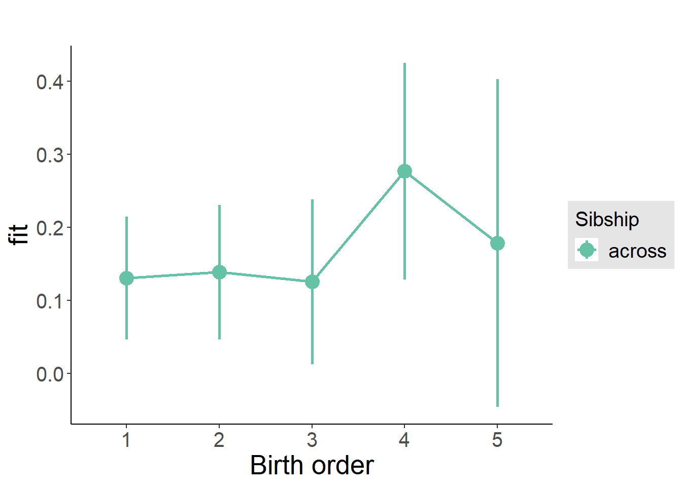
Add Interaction
Model Summary
m4_interaction = update(m3_birthorder_nonlinear, formula = . ~ . - birth_order_nonlinear - sibling_count + count_birth_order)
tidy(m4_interaction, conf.int = T, conf.level = 0.995)| effect | group | term | estimate | std.error | statistic | df | p.value | conf.low | conf.high |
|---|---|---|---|---|---|---|---|---|---|
| fixed | NA | (Intercept) | -1.299 | 0.5268 | -2.465 | 4167 | 0.01373 | -2.778 | 0.18 |
| fixed | NA | poly(age, 3, raw = TRUE)1 | 0.171 | 0.06147 | 2.782 | 4167 | 0.005421 | -0.001519 | 0.3436 |
| fixed | NA | poly(age, 3, raw = TRUE)2 | -0.006321 | 0.002267 | -2.789 | 4166 | 0.005311 | -0.01268 | 0.0000409 |
| fixed | NA | poly(age, 3, raw = TRUE)3 | 0.00007416 | 0.00002657 | 2.791 | 4165 | 0.005271 | -0.0000004136 | 0.0001487 |
| fixed | NA | male | 0.1169 | 0.02854 | 4.096 | 4103 | 0.00004291 | 0.03678 | 0.197 |
| fixed | NA | count_birth_order2/2 | -0.03659 | 0.06139 | -0.596 | 3572 | 0.5512 | -0.2089 | 0.1357 |
| fixed | NA | count_birth_order1/3 | -0.1578 | 0.0537 | -2.939 | 4159 | 0.003307 | -0.3086 | -0.007106 |
| fixed | NA | count_birth_order2/3 | -0.1268 | 0.0582 | -2.179 | 4167 | 0.02942 | -0.2901 | 0.03658 |
| fixed | NA | count_birth_order3/3 | -0.1099 | 0.06548 | -1.679 | 4162 | 0.0933 | -0.2937 | 0.07389 |
| fixed | NA | count_birth_order1/4 | -0.1356 | 0.06373 | -2.128 | 4164 | 0.03343 | -0.3145 | 0.0433 |
| fixed | NA | count_birth_order2/4 | -0.1061 | 0.06483 | -1.637 | 4167 | 0.1017 | -0.2881 | 0.07584 |
| fixed | NA | count_birth_order3/4 | -0.1999 | 0.07105 | -2.813 | 4152 | 0.004928 | -0.3993 | -0.0004374 |
| fixed | NA | count_birth_order4/4 | 0.01211 | 0.07317 | 0.1655 | 4152 | 0.8686 | -0.1933 | 0.2175 |
| fixed | NA | count_birth_order1/5 | -0.1726 | 0.07579 | -2.278 | 4167 | 0.0228 | -0.3854 | 0.04012 |
| fixed | NA | count_birth_order2/5 | -0.1605 | 0.08116 | -1.977 | 4153 | 0.04809 | -0.3883 | 0.06735 |
| fixed | NA | count_birth_order3/5 | -0.1581 | 0.07881 | -2.006 | 4147 | 0.04497 | -0.3793 | 0.06316 |
| fixed | NA | count_birth_order4/5 | -0.03308 | 0.08161 | -0.4053 | 4132 | 0.6853 | -0.2622 | 0.196 |
| fixed | NA | count_birth_order5/5 | -0.1204 | 0.08176 | -1.473 | 4129 | 0.1408 | -0.3499 | 0.1091 |
| ran_pars | mother_pidlink | sd__(Intercept) | 0.3143 | NA | NA | NA | NA | NA | NA |
| ran_pars | Residual | sd__Observation | 0.8709 | NA | NA | NA | NA | NA | NA |
Coefficient Plot
plot_birthorder(m4_interaction)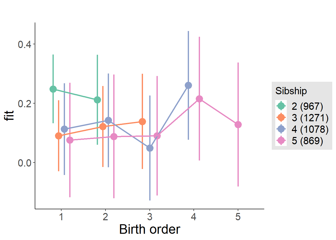
Model Comparison
###### Model 1 - Model 2
anova(m1_covariates_only, m2_birthorder_linear, m3_birthorder_nonlinear, m4_interaction)## refitting model(s) with ML (instead of REML)| Df | AIC | BIC | logLik | deviance | Chisq | Chi Df | Pr(>Chisq) |
|---|---|---|---|---|---|---|---|
| 10 | 11224 | 11287 | -5602 | 11204 | NA | NA | NA |
| 11 | 11223 | 11293 | -5601 | 11201 | 2.422 | 1 | 0.1197 |
| 14 | 11224 | 11313 | -5598 | 11196 | 5.18 | 3 | 0.1591 |
| 20 | 11234 | 11360 | -5597 | 11194 | 2.394 | 6 | 0.8801 |
Parental full sibling order
outcome_parental_m1 <- update(m2_birthorder_linear, data = birthorder %>%
mutate(sibling_count = sibling_count_genes_factor,
birth_order_nonlinear = birthorder_genes_factor,
birth_order = birthorder_genes,
count_birth_order = count_birthorder_genes
) %>%
filter(sibling_count != "1"))
compare_models_markdown(outcome_parental_m1)Basic Model
Model Summary
m1_covariates_only <- update(m2_birthorder_linear, formula = . ~ . - birth_order)
tidy(m1_covariates_only, conf.int = T, conf.level = 0.995)| effect | group | term | estimate | std.error | statistic | df | p.value | conf.low | conf.high |
|---|---|---|---|---|---|---|---|---|---|
| fixed | NA | (Intercept) | -0.9088 | 0.5145 | -1.766 | 4484 | 0.07742 | -2.353 | 0.5355 |
| fixed | NA | poly(age, 3, raw = TRUE)1 | 0.1233 | 0.06013 | 2.051 | 4485 | 0.04037 | -0.04549 | 0.2921 |
| fixed | NA | poly(age, 3, raw = TRUE)2 | -0.004581 | 0.002219 | -2.064 | 4484 | 0.03905 | -0.01081 | 0.001648 |
| fixed | NA | poly(age, 3, raw = TRUE)3 | 0.00005373 | 0.00002605 | 2.062 | 4482 | 0.03924 | -0.0000194 | 0.0001269 |
| fixed | NA | male | 0.1072 | 0.0275 | 3.897 | 4425 | 0.00009896 | 0.02997 | 0.1843 |
| fixed | NA | sibling_count3 | -0.1071 | 0.03702 | -2.894 | 3298 | 0.003829 | -0.2111 | -0.003218 |
| fixed | NA | sibling_count4 | -0.08615 | 0.0402 | -2.143 | 2886 | 0.03219 | -0.199 | 0.02669 |
| fixed | NA | sibling_count5 | -0.09137 | 0.04734 | -1.93 | 2463 | 0.05372 | -0.2243 | 0.04152 |
| ran_pars | mother_pidlink | sd__(Intercept) | 0.3117 | NA | NA | NA | NA | NA | NA |
| ran_pars | Residual | sd__Observation | 0.8708 | NA | NA | NA | NA | NA | NA |
Coefficient Plot
plot(allEffects(m1_covariates_only, confidence.level = 0.995))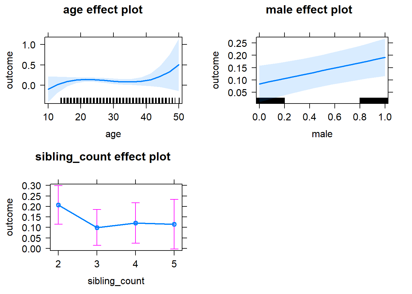
Add Birth Order Linear
Model Summary
tidy(m2_birthorder_linear, conf.int = T, conf.level = 0.995)| effect | group | term | estimate | std.error | statistic | df | p.value | conf.low | conf.high |
|---|---|---|---|---|---|---|---|---|---|
| fixed | NA | (Intercept) | -0.9437 | 0.515 | -1.832 | 4483 | 0.06697 | -2.389 | 0.502 |
| fixed | NA | birth_order | 0.02102 | 0.01459 | 1.44 | 4142 | 0.1498 | -0.01994 | 0.06197 |
| fixed | NA | poly(age, 3, raw = TRUE)1 | 0.1244 | 0.06013 | 2.069 | 4484 | 0.03857 | -0.04436 | 0.2932 |
| fixed | NA | poly(age, 3, raw = TRUE)2 | -0.004646 | 0.002219 | -2.093 | 4483 | 0.03639 | -0.01088 | 0.001584 |
| fixed | NA | poly(age, 3, raw = TRUE)3 | 0.00005491 | 0.00002606 | 2.107 | 4482 | 0.03518 | -0.00001824 | 0.0001281 |
| fixed | NA | male | 0.1066 | 0.0275 | 3.877 | 4425 | 0.0001073 | 0.02942 | 0.1838 |
| fixed | NA | sibling_count3 | -0.1168 | 0.03761 | -3.105 | 3355 | 0.00192 | -0.2223 | -0.0112 |
| fixed | NA | sibling_count4 | -0.1083 | 0.04302 | -2.517 | 3130 | 0.01188 | -0.229 | 0.01247 |
| fixed | NA | sibling_count5 | -0.1268 | 0.05334 | -2.378 | 2932 | 0.01747 | -0.2766 | 0.02289 |
| ran_pars | mother_pidlink | sd__(Intercept) | 0.3105 | NA | NA | NA | NA | NA | NA |
| ran_pars | Residual | sd__Observation | 0.8711 | NA | NA | NA | NA | NA | NA |
Coefficient Plot
plot_birthorder2(m2_birthorder_linear, separate = FALSE)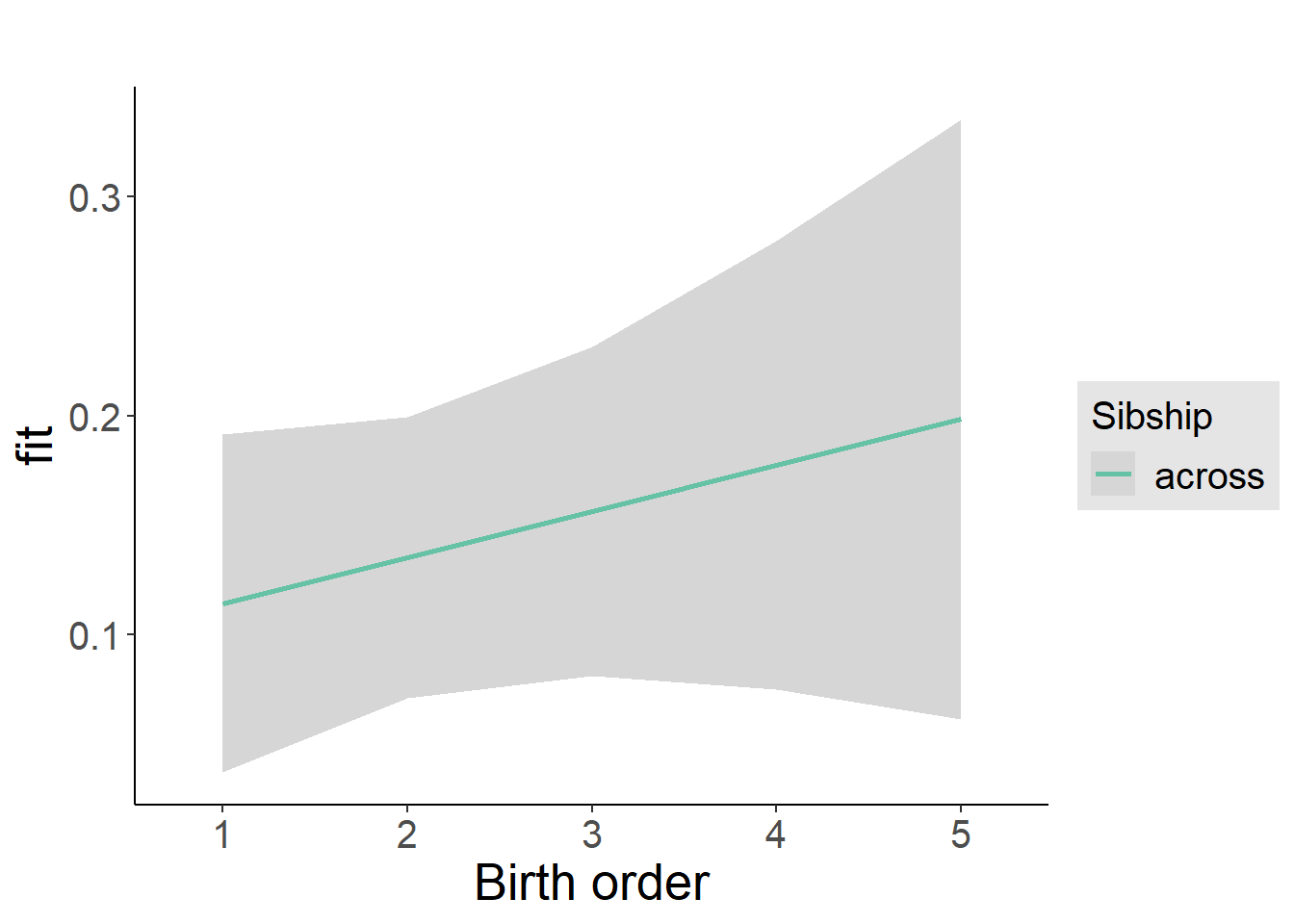
Add Birth Order Factor
Model Summary
m3_birthorder_nonlinear = update(m1_covariates_only, formula = . ~ . + birth_order_nonlinear)
tidy(m3_birthorder_nonlinear, conf.int = T, conf.level = 0.995)| effect | group | term | estimate | std.error | statistic | df | p.value | conf.low | conf.high |
|---|---|---|---|---|---|---|---|---|---|
| fixed | NA | (Intercept) | -0.894 | 0.5156 | -1.734 | 4481 | 0.08298 | -2.341 | 0.5532 |
| fixed | NA | poly(age, 3, raw = TRUE)1 | 0.1216 | 0.0602 | 2.02 | 4481 | 0.04341 | -0.04736 | 0.2906 |
| fixed | NA | poly(age, 3, raw = TRUE)2 | -0.004547 | 0.002222 | -2.046 | 4479 | 0.04078 | -0.01078 | 0.00169 |
| fixed | NA | poly(age, 3, raw = TRUE)3 | 0.00005387 | 0.00002609 | 2.065 | 4477 | 0.03896 | -0.00001935 | 0.0001271 |
| fixed | NA | male | 0.1058 | 0.02751 | 3.847 | 4420 | 0.000121 | 0.02862 | 0.1831 |
| fixed | NA | sibling_count3 | -0.1088 | 0.03823 | -2.847 | 3479 | 0.004444 | -0.2161 | -0.001516 |
| fixed | NA | sibling_count4 | -0.1085 | 0.04368 | -2.485 | 3231 | 0.01301 | -0.2312 | 0.01408 |
| fixed | NA | sibling_count5 | -0.1343 | 0.05444 | -2.467 | 3031 | 0.01367 | -0.2871 | 0.0185 |
| fixed | NA | birth_order_nonlinear2 | 0.007869 | 0.03248 | 0.2423 | 3606 | 0.8086 | -0.08329 | 0.09903 |
| fixed | NA | birth_order_nonlinear3 | 0.005863 | 0.04151 | 0.1413 | 3802 | 0.8877 | -0.1107 | 0.1224 |
| fixed | NA | birth_order_nonlinear4 | 0.09932 | 0.05715 | 1.738 | 3998 | 0.08231 | -0.0611 | 0.2597 |
| fixed | NA | birth_order_nonlinear5 | 0.1052 | 0.09327 | 1.128 | 3943 | 0.2596 | -0.1566 | 0.367 |
| ran_pars | mother_pidlink | sd__(Intercept) | 0.3111 | NA | NA | NA | NA | NA | NA |
| ran_pars | Residual | sd__Observation | 0.871 | NA | NA | NA | NA | NA | NA |
Coefficient Plot
plot_birthorder(m3_birthorder_nonlinear, separate = FALSE)
Add Interaction
Model Summary
m4_interaction = update(m3_birthorder_nonlinear, formula = . ~ . - birth_order_nonlinear - sibling_count + count_birth_order)
tidy(m4_interaction, conf.int = T, conf.level = 0.995)| effect | group | term | estimate | std.error | statistic | df | p.value | conf.low | conf.high |
|---|---|---|---|---|---|---|---|---|---|
| fixed | NA | (Intercept) | -0.8907 | 0.5158 | -1.727 | 4475 | 0.08428 | -2.339 | 0.5572 |
| fixed | NA | poly(age, 3, raw = TRUE)1 | 0.1228 | 0.06023 | 2.039 | 4475 | 0.04148 | -0.04624 | 0.2919 |
| fixed | NA | poly(age, 3, raw = TRUE)2 | -0.004588 | 0.002223 | -2.064 | 4474 | 0.03909 | -0.01083 | 0.001652 |
| fixed | NA | poly(age, 3, raw = TRUE)3 | 0.00005429 | 0.0000261 | 2.08 | 4472 | 0.03758 | -0.00001898 | 0.0001276 |
| fixed | NA | male | 0.1056 | 0.02752 | 3.837 | 4414 | 0.0001265 | 0.02834 | 0.1829 |
| fixed | NA | count_birth_order2/2 | -0.03167 | 0.05463 | -0.5797 | 3768 | 0.5621 | -0.185 | 0.1217 |
| fixed | NA | count_birth_order1/3 | -0.1362 | 0.04895 | -2.781 | 4465 | 0.005437 | -0.2736 | 0.00126 |
| fixed | NA | count_birth_order2/3 | -0.1206 | 0.05409 | -2.229 | 4475 | 0.02585 | -0.2724 | 0.03126 |
| fixed | NA | count_birth_order3/3 | -0.0812 | 0.05941 | -1.367 | 4469 | 0.1718 | -0.248 | 0.08558 |
| fixed | NA | count_birth_order1/4 | -0.1032 | 0.06105 | -1.691 | 4474 | 0.09091 | -0.2746 | 0.06814 |
| fixed | NA | count_birth_order2/4 | -0.1124 | 0.06268 | -1.793 | 4473 | 0.07303 | -0.2883 | 0.06355 |
| fixed | NA | count_birth_order3/4 | -0.1396 | 0.0656 | -2.128 | 4458 | 0.03341 | -0.3237 | 0.04455 |
| fixed | NA | count_birth_order4/4 | -0.02487 | 0.06928 | -0.3589 | 4452 | 0.7197 | -0.2193 | 0.1696 |
| fixed | NA | count_birth_order1/5 | -0.1981 | 0.08246 | -2.402 | 4474 | 0.01633 | -0.4296 | 0.03336 |
| fixed | NA | count_birth_order2/5 | -0.02959 | 0.0909 | -0.3255 | 4448 | 0.7448 | -0.2847 | 0.2256 |
| fixed | NA | count_birth_order3/5 | -0.1846 | 0.08661 | -2.132 | 4442 | 0.03307 | -0.4278 | 0.05848 |
| fixed | NA | count_birth_order4/5 | -0.04553 | 0.08342 | -0.5458 | 4450 | 0.5852 | -0.2797 | 0.1886 |
| fixed | NA | count_birth_order5/5 | -0.04235 | 0.08857 | -0.4781 | 4437 | 0.6326 | -0.291 | 0.2063 |
| ran_pars | mother_pidlink | sd__(Intercept) | 0.3107 | NA | NA | NA | NA | NA | NA |
| ran_pars | Residual | sd__Observation | 0.8713 | NA | NA | NA | NA | NA | NA |
Coefficient Plot
plot_birthorder(m4_interaction)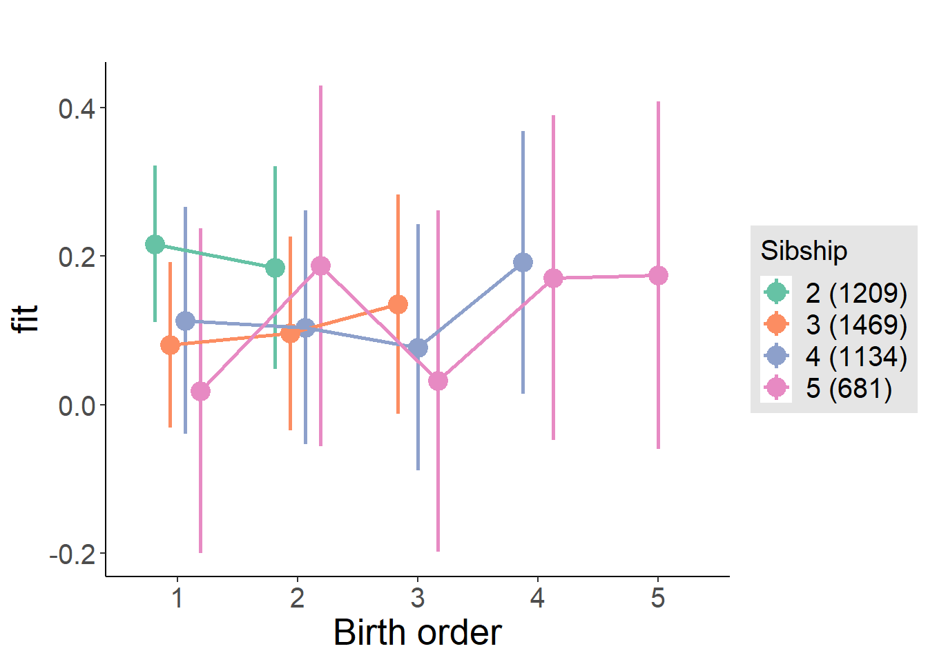
Model Comparison
###### Model 1 - Model 2
anova(m1_covariates_only, m2_birthorder_linear, m3_birthorder_nonlinear, m4_interaction)## refitting model(s) with ML (instead of REML)| Df | AIC | BIC | logLik | deviance | Chisq | Chi Df | Pr(>Chisq) |
|---|---|---|---|---|---|---|---|
| 10 | 12039 | 12103 | -6009 | 12019 | NA | NA | NA |
| 11 | 12039 | 12109 | -6008 | 12017 | 2.08 | 1 | 0.1492 |
| 14 | 12043 | 12133 | -6007 | 12015 | 1.788 | 3 | 0.6175 |
| 20 | 12051 | 12179 | -6005 | 12011 | 4.148 | 6 | 0.6566 |
Compare birth order specifications
library(coefplot)
multiplot(outcome_naive_m1, outcome_preg_m1, outcome_uterus_m1, outcome_parental_m1, dodgeHeight = 0.6,
intercept = FALSE)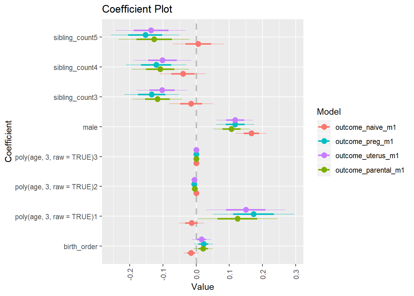
Risk preference
Risk A
birthorder <- birthorder %>% mutate(outcome = riskA)
model = lmer(outcome ~ birth_order + poly(age, 3, raw = TRUE) + male + sibling_count + (1 | mother_pidlink),
data = birthorder)
compare_birthorder_specs(model)Naive birth order
outcome_naive_m1 <- update(m2_birthorder_linear, data = birthorder %>%
mutate(sibling_count = sibling_count_naive_factor,
birth_order_nonlinear = birthorder_naive_factor,
birth_order = birthorder_naive,
count_birth_order = count_birthorder_naive) %>%
filter(sibling_count != "1"))
compare_models_markdown(outcome_naive_m1)Basic Model
Model Summary
m1_covariates_only <- update(m2_birthorder_linear, formula = . ~ . - birth_order)
tidy(m1_covariates_only, conf.int = T, conf.level = 0.995)| effect | group | term | estimate | std.error | statistic | df | p.value | conf.low | conf.high |
|---|---|---|---|---|---|---|---|---|---|
| fixed | NA | (Intercept) | 1.328 | 0.2089 | 6.359 | 5932 | 0.0000000002183 | 0.7418 | 1.914 |
| fixed | NA | poly(age, 3, raw = TRUE)1 | -0.1122 | 0.02005 | -5.597 | 5752 | 0.00000002285 | -0.1685 | -0.05593 |
| fixed | NA | poly(age, 3, raw = TRUE)2 | 0.002981 | 0.0005856 | 5.092 | 5540 | 0.0000003665 | 0.001338 | 0.004625 |
| fixed | NA | poly(age, 3, raw = TRUE)3 | -0.0000239 | 0.000005321 | -4.492 | 5353 | 0.000007215 | -0.00003884 | -0.000008965 |
| fixed | NA | male | -0.2211 | 0.02451 | -9.021 | 6279 | 2.438e-19 | -0.2898 | -0.1523 |
| fixed | NA | sibling_count3 | 0.006697 | 0.03481 | 0.1924 | 4709 | 0.8475 | -0.09103 | 0.1044 |
| fixed | NA | sibling_count4 | 0.009771 | 0.03576 | 0.2733 | 4222 | 0.7846 | -0.0906 | 0.1101 |
| fixed | NA | sibling_count5 | -0.0009568 | 0.03714 | -0.02577 | 3641 | 0.9794 | -0.1052 | 0.1033 |
| ran_pars | mother_pidlink | sd__(Intercept) | 0.2677 | NA | NA | NA | NA | NA | NA |
| ran_pars | Residual | sd__Observation | 0.9415 | NA | NA | NA | NA | NA | NA |
Coefficient Plot
plot(allEffects(m1_covariates_only, confidence.level = 0.995))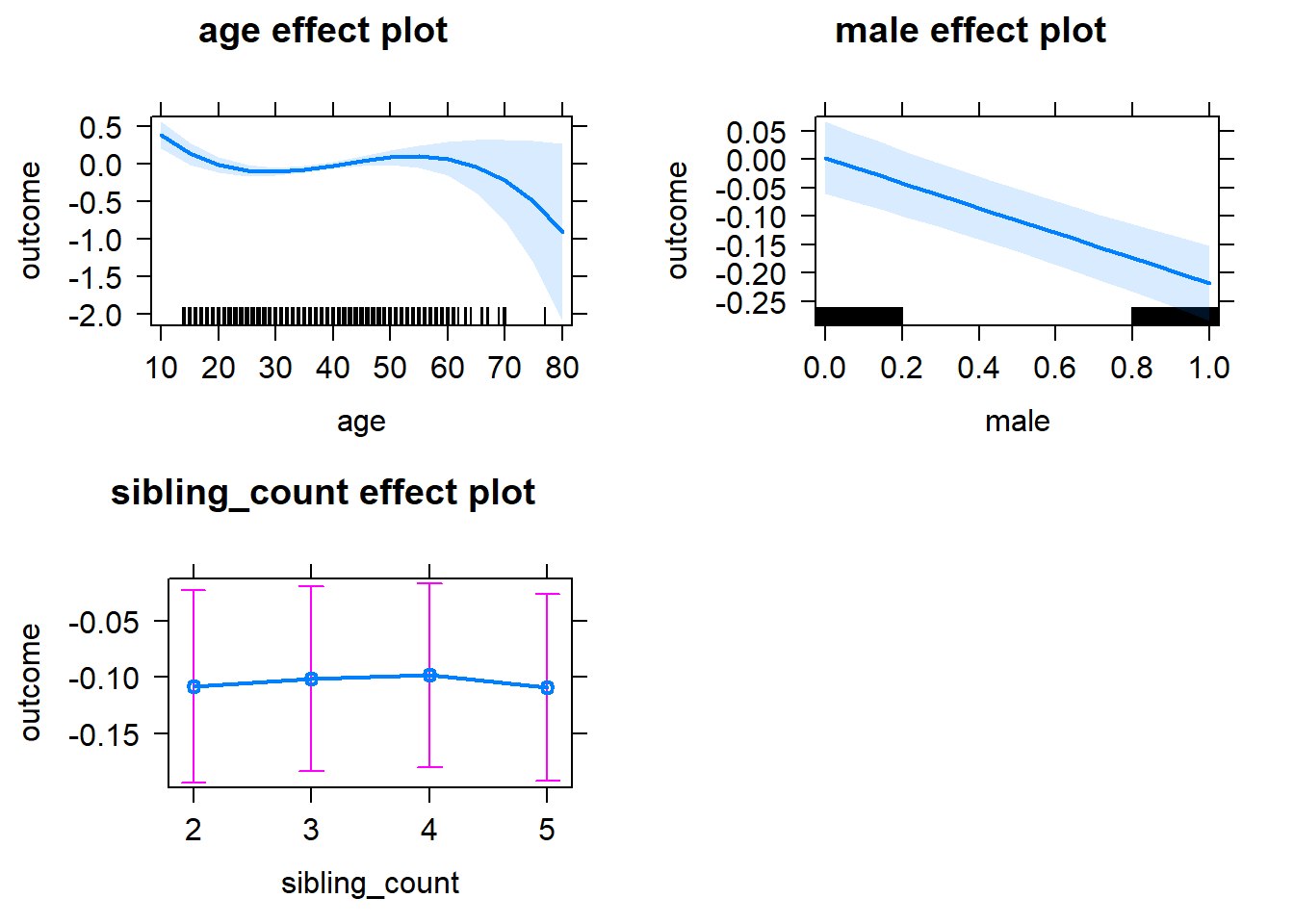
Add Birth Order Linear
Model Summary
tidy(m2_birthorder_linear, conf.int = T, conf.level = 0.995)| effect | group | term | estimate | std.error | statistic | df | p.value | conf.low | conf.high |
|---|---|---|---|---|---|---|---|---|---|
| fixed | NA | (Intercept) | 1.322 | 0.2089 | 6.33 | 5921 | 0.0000000002638 | 0.736 | 1.909 |
| fixed | NA | birth_order | 0.0139 | 0.0123 | 1.13 | 5589 | 0.2586 | -0.02063 | 0.04842 |
| fixed | NA | poly(age, 3, raw = TRUE)1 | -0.1135 | 0.02008 | -5.652 | 5778 | 0.00000001659 | -0.1699 | -0.05714 |
| fixed | NA | poly(age, 3, raw = TRUE)2 | 0.003014 | 0.0005863 | 5.141 | 5554 | 0.0000002819 | 0.001369 | 0.00466 |
| fixed | NA | poly(age, 3, raw = TRUE)3 | -0.00002411 | 0.000005325 | -4.528 | 5361 | 0.000006076 | -0.00003906 | -0.000009165 |
| fixed | NA | male | -0.2214 | 0.02451 | -9.036 | 6277 | 2.134e-19 | -0.2902 | -0.1526 |
| fixed | NA | sibling_count3 | 0.001551 | 0.03511 | 0.04416 | 4819 | 0.9648 | -0.09702 | 0.1001 |
| fixed | NA | sibling_count4 | -0.001851 | 0.03721 | -0.04974 | 4687 | 0.9603 | -0.1063 | 0.1026 |
| fixed | NA | sibling_count5 | -0.02006 | 0.04081 | -0.4916 | 4625 | 0.623 | -0.1346 | 0.0945 |
| ran_pars | mother_pidlink | sd__(Intercept) | 0.2683 | NA | NA | NA | NA | NA | NA |
| ran_pars | Residual | sd__Observation | 0.9413 | NA | NA | NA | NA | NA | NA |
Coefficient Plot
plot_birthorder2(m2_birthorder_linear, separate = FALSE)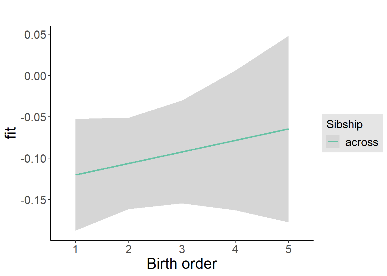
Add Birth Order Factor
Model Summary
m3_birthorder_nonlinear = update(m1_covariates_only, formula = . ~ . + birth_order_nonlinear)
tidy(m3_birthorder_nonlinear, conf.int = T, conf.level = 0.995)| effect | group | term | estimate | std.error | statistic | df | p.value | conf.low | conf.high |
|---|---|---|---|---|---|---|---|---|---|
| fixed | NA | (Intercept) | 1.322 | 0.2095 | 6.312 | 5942 | 0.0000000002954 | 0.7342 | 1.91 |
| fixed | NA | poly(age, 3, raw = TRUE)1 | -0.1126 | 0.02009 | -5.605 | 5764 | 0.00000002175 | -0.169 | -0.05622 |
| fixed | NA | poly(age, 3, raw = TRUE)2 | 0.002993 | 0.0005866 | 5.102 | 5532 | 0.000000347 | 0.001346 | 0.00464 |
| fixed | NA | poly(age, 3, raw = TRUE)3 | -0.00002396 | 0.000005329 | -4.496 | 5329 | 0.000007067 | -0.00003892 | -0.000009002 |
| fixed | NA | male | -0.2218 | 0.0245 | -9.051 | 6274 | 1.852e-19 | -0.2906 | -0.153 |
| fixed | NA | sibling_count3 | 0.003854 | 0.03571 | 0.1079 | 5007 | 0.9141 | -0.09638 | 0.1041 |
| fixed | NA | sibling_count4 | 0.01231 | 0.03783 | 0.3255 | 4890 | 0.7448 | -0.09389 | 0.1185 |
| fixed | NA | sibling_count5 | -0.02412 | 0.04118 | -0.5858 | 4765 | 0.558 | -0.1397 | 0.09146 |
| fixed | NA | birth_order_nonlinear2 | 0.02301 | 0.02931 | 0.785 | 5489 | 0.4325 | -0.05927 | 0.1053 |
| fixed | NA | birth_order_nonlinear3 | 0.02015 | 0.03743 | 0.5383 | 5415 | 0.5904 | -0.08491 | 0.1252 |
| fixed | NA | birth_order_nonlinear4 | -0.02347 | 0.0493 | -0.4762 | 5461 | 0.634 | -0.1618 | 0.1149 |
| fixed | NA | birth_order_nonlinear5 | 0.1614 | 0.07033 | 2.294 | 5340 | 0.02182 | -0.03607 | 0.3588 |
| ran_pars | mother_pidlink | sd__(Intercept) | 0.2672 | NA | NA | NA | NA | NA | NA |
| ran_pars | Residual | sd__Observation | 0.9414 | NA | NA | NA | NA | NA | NA |
Coefficient Plot
plot_birthorder(m3_birthorder_nonlinear, separate = FALSE)
Add Interaction
Model Summary
m4_interaction = update(m3_birthorder_nonlinear, formula = . ~ . - birth_order_nonlinear - sibling_count + count_birth_order)
tidy(m4_interaction, conf.int = T, conf.level = 0.995)| effect | group | term | estimate | std.error | statistic | df | p.value | conf.low | conf.high |
|---|---|---|---|---|---|---|---|---|---|
| fixed | NA | (Intercept) | 1.342 | 0.2097 | 6.402 | 5943 | 0.0000000001656 | 0.7537 | 1.931 |
| fixed | NA | poly(age, 3, raw = TRUE)1 | -0.1137 | 0.02007 | -5.665 | 5759 | 0.00000001542 | -0.17 | -0.05735 |
| fixed | NA | poly(age, 3, raw = TRUE)2 | 0.003016 | 0.0005859 | 5.147 | 5524 | 0.000000274 | 0.001371 | 0.00466 |
| fixed | NA | poly(age, 3, raw = TRUE)3 | -0.00002408 | 0.000005323 | -4.524 | 5317 | 0.000006186 | -0.00003903 | -0.000009142 |
| fixed | NA | male | -0.2232 | 0.02448 | -9.115 | 6268 | 1.042e-19 | -0.2919 | -0.1544 |
| fixed | NA | count_birth_order2/2 | 0.006423 | 0.04974 | 0.1291 | 5441 | 0.8973 | -0.1332 | 0.146 |
| fixed | NA | count_birth_order1/3 | -0.04722 | 0.04671 | -1.011 | 6330 | 0.3121 | -0.1783 | 0.08389 |
| fixed | NA | count_birth_order2/3 | 0.03383 | 0.05272 | 0.6418 | 6336 | 0.5211 | -0.1141 | 0.1818 |
| fixed | NA | count_birth_order3/3 | 0.09029 | 0.05814 | 1.553 | 6336 | 0.1205 | -0.0729 | 0.2535 |
| fixed | NA | count_birth_order1/4 | 0.0577 | 0.05335 | 1.081 | 6336 | 0.2796 | -0.09207 | 0.2075 |
| fixed | NA | count_birth_order2/4 | -0.01205 | 0.05597 | -0.2154 | 6337 | 0.8295 | -0.1691 | 0.145 |
| fixed | NA | count_birth_order3/4 | -0.08298 | 0.06069 | -1.367 | 6335 | 0.1716 | -0.2534 | 0.08739 |
| fixed | NA | count_birth_order4/4 | 0.08942 | 0.06526 | 1.37 | 6330 | 0.1707 | -0.09378 | 0.2726 |
| fixed | NA | count_birth_order1/5 | -0.02227 | 0.06135 | -0.3629 | 6336 | 0.7167 | -0.1945 | 0.1499 |
| fixed | NA | count_birth_order2/5 | 0.05073 | 0.06339 | 0.8002 | 6333 | 0.4236 | -0.1272 | 0.2287 |
| fixed | NA | count_birth_order3/5 | 0.02637 | 0.06549 | 0.4026 | 6327 | 0.6872 | -0.1575 | 0.2102 |
| fixed | NA | count_birth_order4/5 | -0.1776 | 0.06933 | -2.562 | 6323 | 0.01042 | -0.3722 | 0.01697 |
| fixed | NA | count_birth_order5/5 | 0.1312 | 0.06982 | 1.88 | 6323 | 0.0602 | -0.06475 | 0.3272 |
| ran_pars | mother_pidlink | sd__(Intercept) | 0.2652 | NA | NA | NA | NA | NA | NA |
| ran_pars | Residual | sd__Observation | 0.9408 | NA | NA | NA | NA | NA | NA |
Coefficient Plot
plot_birthorder(m4_interaction)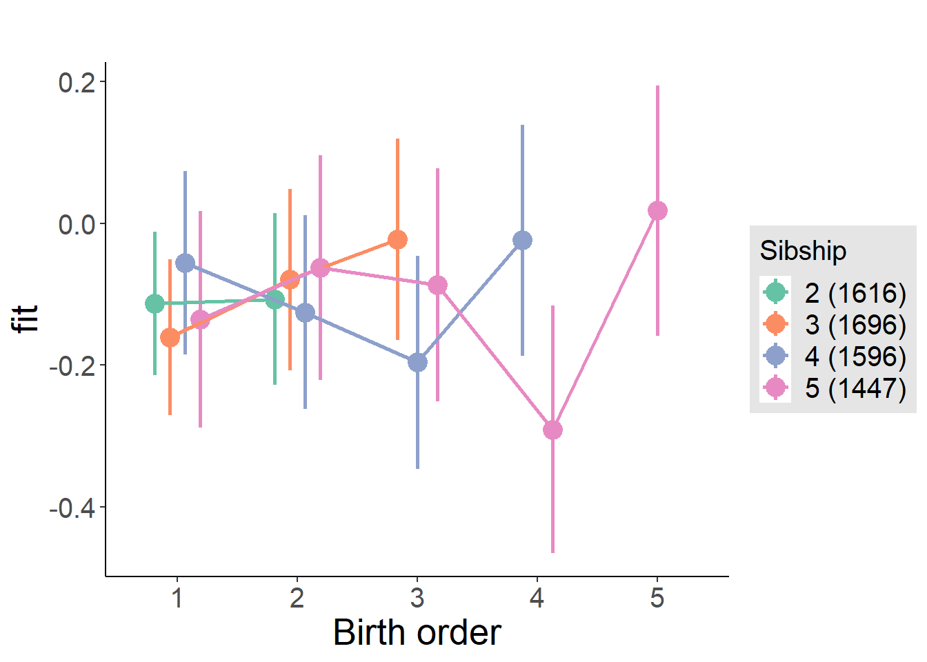
Model Comparison
###### Model 1 - Model 2
anova(m1_covariates_only, m2_birthorder_linear, m3_birthorder_nonlinear, m4_interaction)## refitting model(s) with ML (instead of REML)| Df | AIC | BIC | logLik | deviance | Chisq | Chi Df | Pr(>Chisq) |
|---|---|---|---|---|---|---|---|
| 10 | 17760 | 17827 | -8870 | 17740 | NA | NA | NA |
| 11 | 17760 | 17835 | -8869 | 17738 | 1.276 | 1 | 0.2586 |
| 14 | 17761 | 17856 | -8867 | 17733 | 5.409 | 3 | 0.1442 |
| 20 | 17753 | 17888 | -8856 | 17713 | 20.33 | 6 | 0.002418 |
Maternal birth order
outcome_uterus_m1 <- update(m2_birthorder_linear, data = birthorder %>%
mutate(sibling_count = sibling_count_uterus_alive_factor,
birth_order_nonlinear = birthorder_uterus_alive_factor,
birth_order = birthorder_uterus_alive,
count_birth_order = count_birthorder_uterus_alive) %>%
filter(sibling_count != "1"))
compare_models_markdown(outcome_uterus_m1)Basic Model
Model Summary
m1_covariates_only <- update(m2_birthorder_linear, formula = . ~ . - birth_order)
tidy(m1_covariates_only, conf.int = T, conf.level = 0.995)| effect | group | term | estimate | std.error | statistic | df | p.value | conf.low | conf.high |
|---|---|---|---|---|---|---|---|---|---|
| fixed | NA | (Intercept) | 2.028 | 0.5514 | 3.678 | 4061 | 0.0002378 | 0.4805 | 3.576 |
| fixed | NA | poly(age, 3, raw = TRUE)1 | -0.1893 | 0.06434 | -2.943 | 4059 | 0.003271 | -0.3699 | -0.008733 |
| fixed | NA | poly(age, 3, raw = TRUE)2 | 0.005631 | 0.00237 | 2.376 | 4056 | 0.01756 | -0.001022 | 0.01228 |
| fixed | NA | poly(age, 3, raw = TRUE)3 | -0.00005467 | 0.00002776 | -1.969 | 4052 | 0.04902 | -0.0001326 | 0.00002327 |
| fixed | NA | male | -0.254 | 0.02984 | -8.512 | 4031 | 2.37e-17 | -0.3378 | -0.1703 |
| fixed | NA | sibling_count3 | -0.01577 | 0.04021 | -0.3922 | 3139 | 0.6949 | -0.1286 | 0.09709 |
| fixed | NA | sibling_count4 | 0.01271 | 0.04337 | 0.2931 | 2741 | 0.7695 | -0.109 | 0.1344 |
| fixed | NA | sibling_count5 | 0.0296 | 0.04917 | 0.602 | 2429 | 0.5472 | -0.1084 | 0.1676 |
| ran_pars | mother_pidlink | sd__(Intercept) | 0.2636 | NA | NA | NA | NA | NA | NA |
| ran_pars | Residual | sd__Observation | 0.916 | NA | NA | NA | NA | NA | NA |
Coefficient Plot
plot(allEffects(m1_covariates_only, confidence.level = 0.995))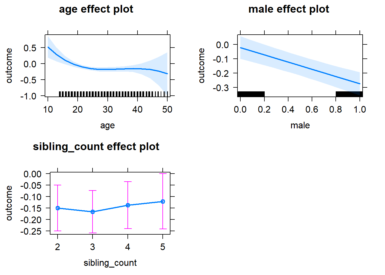
Add Birth Order Linear
Model Summary
tidy(m2_birthorder_linear, conf.int = T, conf.level = 0.995)| effect | group | term | estimate | std.error | statistic | df | p.value | conf.low | conf.high |
|---|---|---|---|---|---|---|---|---|---|
| fixed | NA | (Intercept) | 2.015 | 0.5525 | 3.648 | 4060 | 0.000268 | 0.4644 | 3.566 |
| fixed | NA | birth_order | 0.006387 | 0.0157 | 0.4067 | 3833 | 0.6842 | -0.03769 | 0.05047 |
| fixed | NA | poly(age, 3, raw = TRUE)1 | -0.1887 | 0.06436 | -2.931 | 4058 | 0.003396 | -0.3693 | -0.007987 |
| fixed | NA | poly(age, 3, raw = TRUE)2 | 0.005599 | 0.002372 | 2.361 | 4055 | 0.01828 | -0.001058 | 0.01226 |
| fixed | NA | poly(age, 3, raw = TRUE)3 | -0.00005417 | 0.00002779 | -1.949 | 4052 | 0.05136 | -0.0001322 | 0.00002385 |
| fixed | NA | male | -0.2542 | 0.02985 | -8.517 | 4030 | 2.28e-17 | -0.338 | -0.1704 |
| fixed | NA | sibling_count3 | -0.01881 | 0.0409 | -0.4598 | 3194 | 0.6457 | -0.1336 | 0.096 |
| fixed | NA | sibling_count4 | 0.005779 | 0.0466 | 0.124 | 2965 | 0.9013 | -0.125 | 0.1366 |
| fixed | NA | sibling_count5 | 0.01818 | 0.05664 | 0.3209 | 2896 | 0.7483 | -0.1408 | 0.1772 |
| ran_pars | mother_pidlink | sd__(Intercept) | 0.2637 | NA | NA | NA | NA | NA | NA |
| ran_pars | Residual | sd__Observation | 0.9161 | NA | NA | NA | NA | NA | NA |
Coefficient Plot
plot_birthorder2(m2_birthorder_linear, separate = FALSE)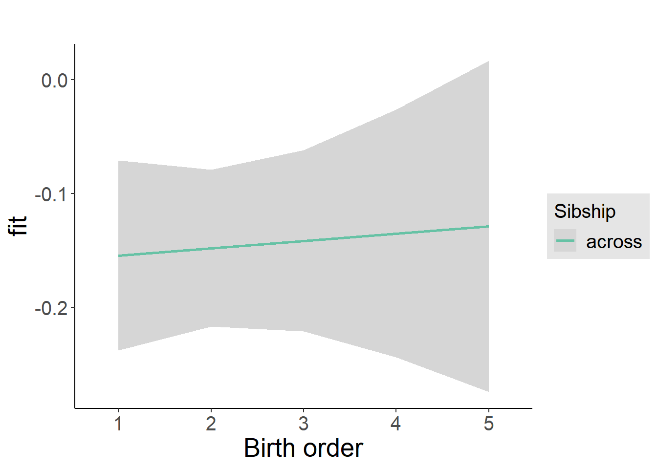
Add Birth Order Factor
Model Summary
m3_birthorder_nonlinear = update(m1_covariates_only, formula = . ~ . + birth_order_nonlinear)
tidy(m3_birthorder_nonlinear, conf.int = T, conf.level = 0.995)| effect | group | term | estimate | std.error | statistic | df | p.value | conf.low | conf.high |
|---|---|---|---|---|---|---|---|---|---|
| fixed | NA | (Intercept) | 2.002 | 0.5529 | 3.621 | 4055 | 0.0002971 | 0.4501 | 3.554 |
| fixed | NA | poly(age, 3, raw = TRUE)1 | -0.1865 | 0.06444 | -2.894 | 4053 | 0.003823 | -0.3674 | -0.005612 |
| fixed | NA | poly(age, 3, raw = TRUE)2 | 0.005519 | 0.002375 | 2.324 | 4050 | 0.02016 | -0.001147 | 0.01219 |
| fixed | NA | poly(age, 3, raw = TRUE)3 | -0.00005329 | 0.00002783 | -1.915 | 4047 | 0.05557 | -0.0001314 | 0.00002482 |
| fixed | NA | male | -0.2541 | 0.02986 | -8.51 | 4027 | 2.427e-17 | -0.3379 | -0.1703 |
| fixed | NA | sibling_count3 | -0.02659 | 0.04163 | -0.6388 | 3298 | 0.523 | -0.1435 | 0.09026 |
| fixed | NA | sibling_count4 | -0.000964 | 0.04731 | -0.02038 | 3053 | 0.9837 | -0.1338 | 0.1318 |
| fixed | NA | sibling_count5 | 0.02667 | 0.05762 | 0.4628 | 2971 | 0.6435 | -0.1351 | 0.1884 |
| fixed | NA | birth_order_nonlinear2 | 0.01214 | 0.03597 | 0.3374 | 3431 | 0.7358 | -0.08884 | 0.1131 |
| fixed | NA | birth_order_nonlinear3 | 0.04638 | 0.04565 | 1.016 | 3592 | 0.3098 | -0.08177 | 0.1745 |
| fixed | NA | birth_order_nonlinear4 | 0.019 | 0.06061 | 0.3135 | 3725 | 0.7539 | -0.1511 | 0.1891 |
| fixed | NA | birth_order_nonlinear5 | -0.04188 | 0.09446 | -0.4434 | 3658 | 0.6575 | -0.307 | 0.2233 |
| ran_pars | mother_pidlink | sd__(Intercept) | 0.2637 | NA | NA | NA | NA | NA | NA |
| ran_pars | Residual | sd__Observation | 0.9163 | NA | NA | NA | NA | NA | NA |
Coefficient Plot
plot_birthorder(m3_birthorder_nonlinear, separate = FALSE)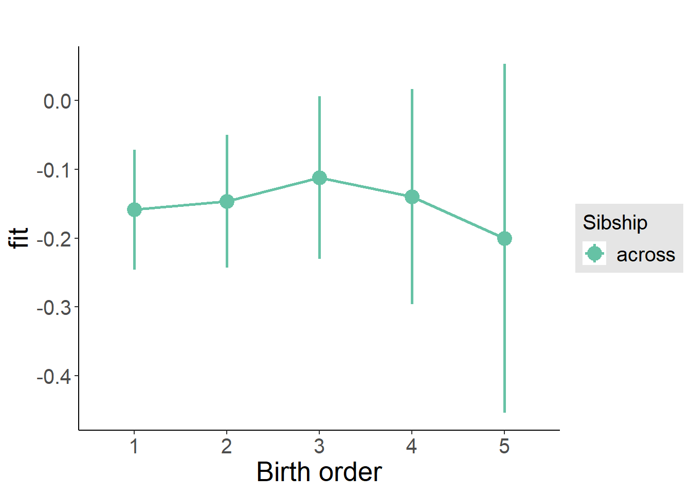
Add Interaction
Model Summary
m4_interaction = update(m3_birthorder_nonlinear, formula = . ~ . - birth_order_nonlinear - sibling_count + count_birth_order)
tidy(m4_interaction, conf.int = T, conf.level = 0.995)| effect | group | term | estimate | std.error | statistic | df | p.value | conf.low | conf.high |
|---|---|---|---|---|---|---|---|---|---|
| fixed | NA | (Intercept) | 1.977 | 0.5528 | 3.575 | 4050 | 0.000354 | 0.4247 | 3.528 |
| fixed | NA | poly(age, 3, raw = TRUE)1 | -0.1839 | 0.06443 | -2.854 | 4048 | 0.004336 | -0.3648 | -0.003042 |
| fixed | NA | poly(age, 3, raw = TRUE)2 | 0.005478 | 0.002374 | 2.307 | 4045 | 0.0211 | -0.001187 | 0.01214 |
| fixed | NA | poly(age, 3, raw = TRUE)3 | -0.00005347 | 0.00002782 | -1.922 | 4042 | 0.05471 | -0.0001316 | 0.00002463 |
| fixed | NA | male | -0.2538 | 0.02987 | -8.495 | 4019 | 2.742e-17 | -0.3376 | -0.1699 |
| fixed | NA | count_birth_order2/2 | -0.0102 | 0.06112 | -0.1669 | 3557 | 0.8674 | -0.1818 | 0.1614 |
| fixed | NA | count_birth_order1/3 | -0.09999 | 0.05377 | -1.86 | 4048 | 0.063 | -0.2509 | 0.05094 |
| fixed | NA | count_birth_order2/3 | 0.01397 | 0.05878 | 0.2376 | 4051 | 0.8122 | -0.151 | 0.179 |
| fixed | NA | count_birth_order3/3 | 0.08693 | 0.06491 | 1.339 | 4049 | 0.1805 | -0.09526 | 0.2691 |
| fixed | NA | count_birth_order1/4 | 0.05852 | 0.06668 | 0.8776 | 4050 | 0.3802 | -0.1287 | 0.2457 |
| fixed | NA | count_birth_order2/4 | -0.01142 | 0.06792 | -0.1681 | 4051 | 0.8665 | -0.2021 | 0.1792 |
| fixed | NA | count_birth_order3/4 | -0.03839 | 0.0724 | -0.5302 | 4042 | 0.596 | -0.2416 | 0.1649 |
| fixed | NA | count_birth_order4/4 | 0.01923 | 0.07359 | 0.2614 | 4042 | 0.7938 | -0.1873 | 0.2258 |
| fixed | NA | count_birth_order1/5 | 0.1145 | 0.09004 | 1.272 | 4050 | 0.2035 | -0.1382 | 0.3673 |
| fixed | NA | count_birth_order2/5 | -0.01591 | 0.09641 | -0.1651 | 4041 | 0.8689 | -0.2865 | 0.2547 |
| fixed | NA | count_birth_order3/5 | 0.0272 | 0.08955 | 0.3038 | 4035 | 0.7613 | -0.2242 | 0.2786 |
| fixed | NA | count_birth_order4/5 | 0.02233 | 0.08533 | 0.2617 | 4041 | 0.7936 | -0.2172 | 0.2619 |
| fixed | NA | count_birth_order5/5 | -0.02365 | 0.08877 | -0.2664 | 4033 | 0.7899 | -0.2728 | 0.2255 |
| ran_pars | mother_pidlink | sd__(Intercept) | 0.2671 | NA | NA | NA | NA | NA | NA |
| ran_pars | Residual | sd__Observation | 0.9148 | NA | NA | NA | NA | NA | NA |
Coefficient Plot
plot_birthorder(m4_interaction)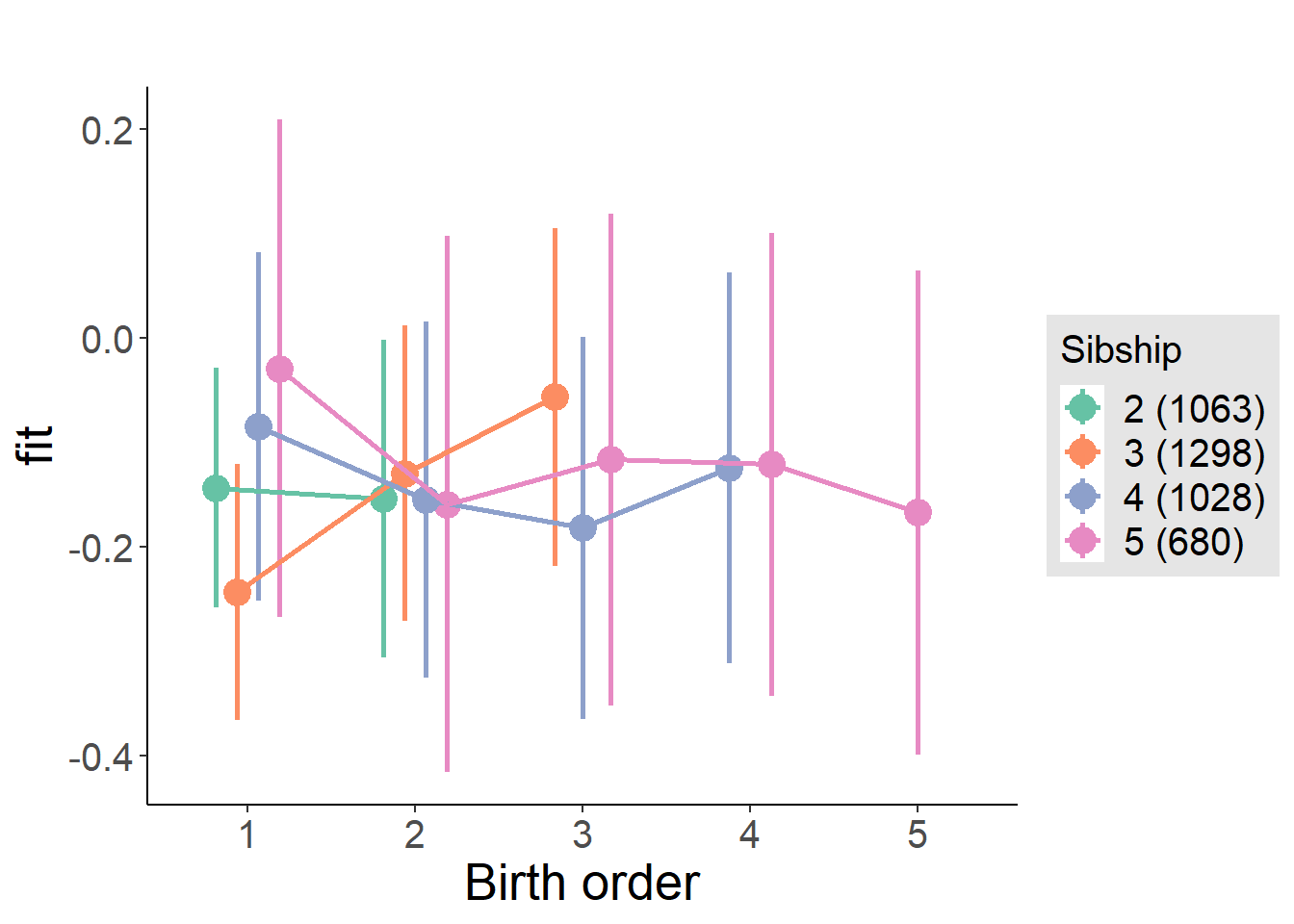
Model Comparison
###### Model 1 - Model 2
anova(m1_covariates_only, m2_birthorder_linear, m3_birthorder_nonlinear, m4_interaction)## refitting model(s) with ML (instead of REML)| Df | AIC | BIC | logLik | deviance | Chisq | Chi Df | Pr(>Chisq) |
|---|---|---|---|---|---|---|---|
| 10 | 11161 | 11224 | -5570 | 11141 | NA | NA | NA |
| 11 | 11163 | 11232 | -5570 | 11141 | 0.1654 | 1 | 0.6843 |
| 14 | 11167 | 11256 | -5570 | 11139 | 1.346 | 3 | 0.7183 |
| 20 | 11169 | 11295 | -5564 | 11129 | 10.56 | 6 | 0.1028 |
Maternal pregnancy order
outcome_preg_m1 <- update(m2_birthorder_linear, data = birthorder %>%
mutate(sibling_count = sibling_count_uterus_preg_factor,
birth_order_nonlinear = birthorder_uterus_preg_factor,
birth_order = birthorder_uterus_preg,
count_birth_order = count_birthorder_uterus_preg
) %>%
filter(sibling_count != "1"))
compare_models_markdown(outcome_preg_m1)Basic Model
Model Summary
m1_covariates_only <- update(m2_birthorder_linear, formula = . ~ . - birth_order)
tidy(m1_covariates_only, conf.int = T, conf.level = 0.995)| effect | group | term | estimate | std.error | statistic | df | p.value | conf.low | conf.high |
|---|---|---|---|---|---|---|---|---|---|
| fixed | NA | (Intercept) | 1.983 | 0.5677 | 3.493 | 3773 | 0.0004837 | 0.3892 | 3.576 |
| fixed | NA | poly(age, 3, raw = TRUE)1 | -0.1863 | 0.06631 | -2.81 | 3771 | 0.004976 | -0.3725 | -0.0002106 |
| fixed | NA | poly(age, 3, raw = TRUE)2 | 0.005679 | 0.002444 | 2.324 | 3767 | 0.02019 | -0.001181 | 0.01254 |
| fixed | NA | poly(age, 3, raw = TRUE)3 | -0.00005659 | 0.00002863 | -1.976 | 3762 | 0.04819 | -0.000137 | 0.00002378 |
| fixed | NA | male | -0.2582 | 0.031 | -8.328 | 3751 | 1.139e-16 | -0.3452 | -0.1712 |
| fixed | NA | sibling_count3 | -0.03455 | 0.04332 | -0.7976 | 2967 | 0.4252 | -0.1562 | 0.08705 |
| fixed | NA | sibling_count4 | -0.03858 | 0.04563 | -0.8456 | 2663 | 0.3978 | -0.1667 | 0.08949 |
| fixed | NA | sibling_count5 | 0.02217 | 0.04852 | 0.4569 | 2366 | 0.6478 | -0.114 | 0.1584 |
| ran_pars | mother_pidlink | sd__(Intercept) | 0.2248 | NA | NA | NA | NA | NA | NA |
| ran_pars | Residual | sd__Observation | 0.926 | NA | NA | NA | NA | NA | NA |
Coefficient Plot
plot(allEffects(m1_covariates_only, confidence.level = 0.995))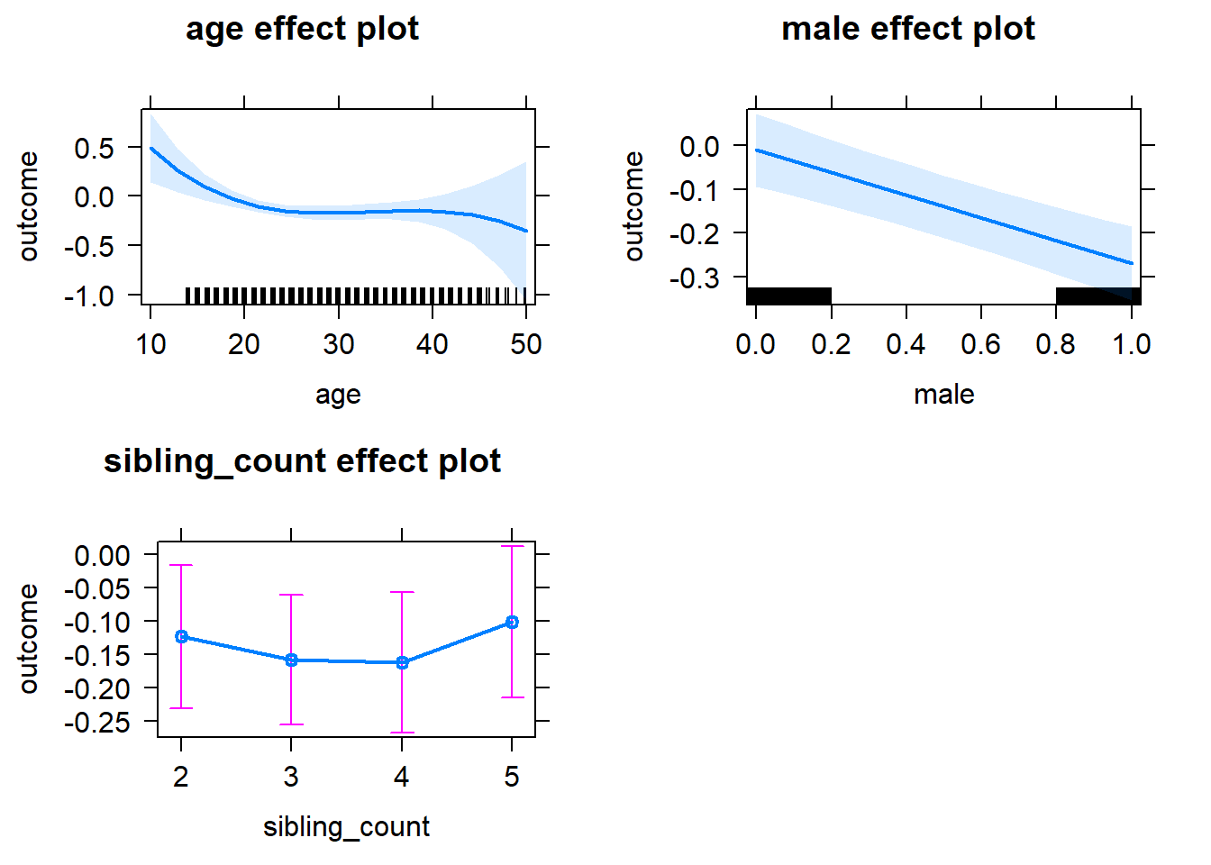
Add Birth Order Linear
Model Summary
tidy(m2_birthorder_linear, conf.int = T, conf.level = 0.995)| effect | group | term | estimate | std.error | statistic | df | p.value | conf.low | conf.high |
|---|---|---|---|---|---|---|---|---|---|
| fixed | NA | (Intercept) | 1.95 | 0.5686 | 3.429 | 3772 | 0.0006123 | 0.3537 | 3.546 |
| fixed | NA | birth_order | 0.01603 | 0.01571 | 1.021 | 3630 | 0.3075 | -0.02806 | 0.06012 |
| fixed | NA | poly(age, 3, raw = TRUE)1 | -0.1847 | 0.06632 | -2.785 | 3770 | 0.00538 | -0.3709 | 0.001462 |
| fixed | NA | poly(age, 3, raw = TRUE)2 | 0.005602 | 0.002445 | 2.291 | 3766 | 0.022 | -0.001261 | 0.01247 |
| fixed | NA | poly(age, 3, raw = TRUE)3 | -0.00005538 | 0.00002866 | -1.933 | 3763 | 0.05336 | -0.0001358 | 0.00002506 |
| fixed | NA | male | -0.2584 | 0.031 | -8.335 | 3749 | 1.075e-16 | -0.3454 | -0.1714 |
| fixed | NA | sibling_count3 | -0.04213 | 0.04395 | -0.9584 | 3003 | 0.3379 | -0.1655 | 0.08125 |
| fixed | NA | sibling_count4 | -0.05529 | 0.04848 | -1.141 | 2825 | 0.2542 | -0.1914 | 0.08079 |
| fixed | NA | sibling_count5 | -0.0042 | 0.05498 | -0.0764 | 2738 | 0.9391 | -0.1585 | 0.1501 |
| ran_pars | mother_pidlink | sd__(Intercept) | 0.2251 | NA | NA | NA | NA | NA | NA |
| ran_pars | Residual | sd__Observation | 0.926 | NA | NA | NA | NA | NA | NA |
Coefficient Plot
plot_birthorder2(m2_birthorder_linear, separate = FALSE)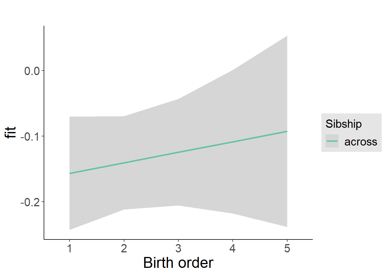
Add Birth Order Factor
Model Summary
m3_birthorder_nonlinear = update(m1_covariates_only, formula = . ~ . + birth_order_nonlinear)
tidy(m3_birthorder_nonlinear, conf.int = T, conf.level = 0.995)| effect | group | term | estimate | std.error | statistic | df | p.value | conf.low | conf.high |
|---|---|---|---|---|---|---|---|---|---|
| fixed | NA | (Intercept) | 1.94 | 0.5687 | 3.412 | 3767 | 0.0006512 | 0.3441 | 3.537 |
| fixed | NA | poly(age, 3, raw = TRUE)1 | -0.1814 | 0.06635 | -2.734 | 3765 | 0.006287 | -0.3676 | 0.004848 |
| fixed | NA | poly(age, 3, raw = TRUE)2 | 0.005473 | 0.002446 | 2.238 | 3761 | 0.02531 | -0.001393 | 0.01234 |
| fixed | NA | poly(age, 3, raw = TRUE)3 | -0.00005388 | 0.00002866 | -1.88 | 3757 | 0.06023 | -0.0001343 | 0.00002658 |
| fixed | NA | male | -0.2589 | 0.03099 | -8.356 | 3746 | 8.994e-17 | -0.3459 | -0.172 |
| fixed | NA | sibling_count3 | -0.05967 | 0.04467 | -1.336 | 3093 | 0.1818 | -0.1851 | 0.06573 |
| fixed | NA | sibling_count4 | -0.07538 | 0.0492 | -1.532 | 2910 | 0.1256 | -0.2135 | 0.06272 |
| fixed | NA | sibling_count5 | 0.005539 | 0.05553 | 0.09975 | 2788 | 0.9206 | -0.1503 | 0.1614 |
| fixed | NA | birth_order_nonlinear2 | 0.0166 | 0.03749 | 0.4427 | 3229 | 0.658 | -0.08864 | 0.1218 |
| fixed | NA | birth_order_nonlinear3 | 0.1088 | 0.04726 | 2.301 | 3413 | 0.02144 | -0.02391 | 0.2414 |
| fixed | NA | birth_order_nonlinear4 | 0.07073 | 0.06167 | 1.147 | 3527 | 0.2515 | -0.1024 | 0.2438 |
| fixed | NA | birth_order_nonlinear5 | -0.08802 | 0.09004 | -0.9776 | 3446 | 0.3284 | -0.3408 | 0.1647 |
| ran_pars | mother_pidlink | sd__(Intercept) | 0.2269 | NA | NA | NA | NA | NA | NA |
| ran_pars | Residual | sd__Observation | 0.925 | NA | NA | NA | NA | NA | NA |
Coefficient Plot
plot_birthorder(m3_birthorder_nonlinear, separate = FALSE)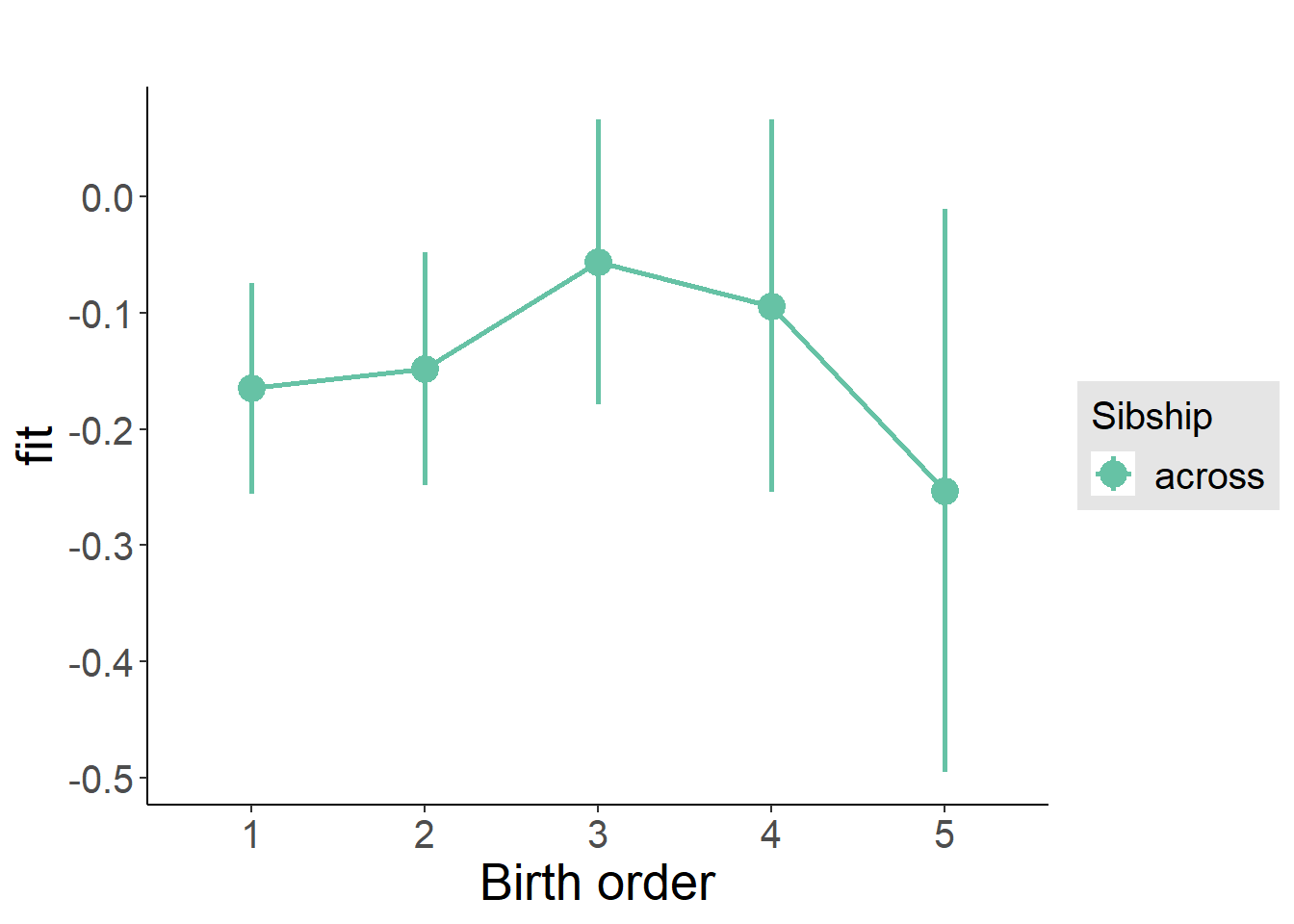
Add Interaction
Model Summary
m4_interaction = update(m3_birthorder_nonlinear, formula = . ~ . - birth_order_nonlinear - sibling_count + count_birth_order)
tidy(m4_interaction, conf.int = T, conf.level = 0.995)| effect | group | term | estimate | std.error | statistic | df | p.value | conf.low | conf.high |
|---|---|---|---|---|---|---|---|---|---|
| fixed | NA | (Intercept) | 1.922 | 0.569 | 3.378 | 3762 | 0.0007367 | 0.3251 | 3.519 |
| fixed | NA | poly(age, 3, raw = TRUE)1 | -0.1786 | 0.06635 | -2.691 | 3759 | 0.007158 | -0.3648 | 0.007706 |
| fixed | NA | poly(age, 3, raw = TRUE)2 | 0.005399 | 0.002446 | 2.207 | 3756 | 0.02737 | -0.001468 | 0.01227 |
| fixed | NA | poly(age, 3, raw = TRUE)3 | -0.00005336 | 0.00002867 | -1.861 | 3752 | 0.06278 | -0.0001338 | 0.00002711 |
| fixed | NA | male | -0.2588 | 0.03101 | -8.345 | 3738 | 9.861e-17 | -0.3458 | -0.1717 |
| fixed | NA | count_birth_order2/2 | -0.02025 | 0.06678 | -0.3033 | 3322 | 0.7617 | -0.2077 | 0.1672 |
| fixed | NA | count_birth_order1/3 | -0.1425 | 0.05828 | -2.446 | 3763 | 0.0145 | -0.3061 | 0.02105 |
| fixed | NA | count_birth_order2/3 | 0.002635 | 0.06296 | 0.04185 | 3764 | 0.9666 | -0.1741 | 0.1794 |
| fixed | NA | count_birth_order3/3 | 0.08658 | 0.07058 | 1.227 | 3762 | 0.22 | -0.1115 | 0.2847 |
| fixed | NA | count_birth_order1/4 | -0.009103 | 0.06939 | -0.1312 | 3763 | 0.8956 | -0.2039 | 0.1857 |
| fixed | NA | count_birth_order2/4 | -0.1244 | 0.07015 | -1.774 | 3764 | 0.0762 | -0.3213 | 0.07249 |
| fixed | NA | count_birth_order3/4 | -0.0441 | 0.07739 | -0.5698 | 3759 | 0.5688 | -0.2613 | 0.1731 |
| fixed | NA | count_birth_order4/4 | 0.007852 | 0.0779 | 0.1008 | 3759 | 0.9197 | -0.2108 | 0.2265 |
| fixed | NA | count_birth_order1/5 | 0.01982 | 0.08191 | 0.242 | 3764 | 0.8088 | -0.2101 | 0.2497 |
| fixed | NA | count_birth_order2/5 | 0.01078 | 0.08836 | 0.122 | 3762 | 0.9029 | -0.2373 | 0.2588 |
| fixed | NA | count_birth_order3/5 | 0.1027 | 0.08474 | 1.212 | 3759 | 0.2257 | -0.1352 | 0.3405 |
| fixed | NA | count_birth_order4/5 | 0.02752 | 0.08779 | 0.3135 | 3754 | 0.754 | -0.2189 | 0.2739 |
| fixed | NA | count_birth_order5/5 | -0.09559 | 0.08723 | -1.096 | 3750 | 0.2732 | -0.3404 | 0.1493 |
| ran_pars | mother_pidlink | sd__(Intercept) | 0.2298 | NA | NA | NA | NA | NA | NA |
| ran_pars | Residual | sd__Observation | 0.9238 | NA | NA | NA | NA | NA | NA |
Coefficient Plot
plot_birthorder(m4_interaction)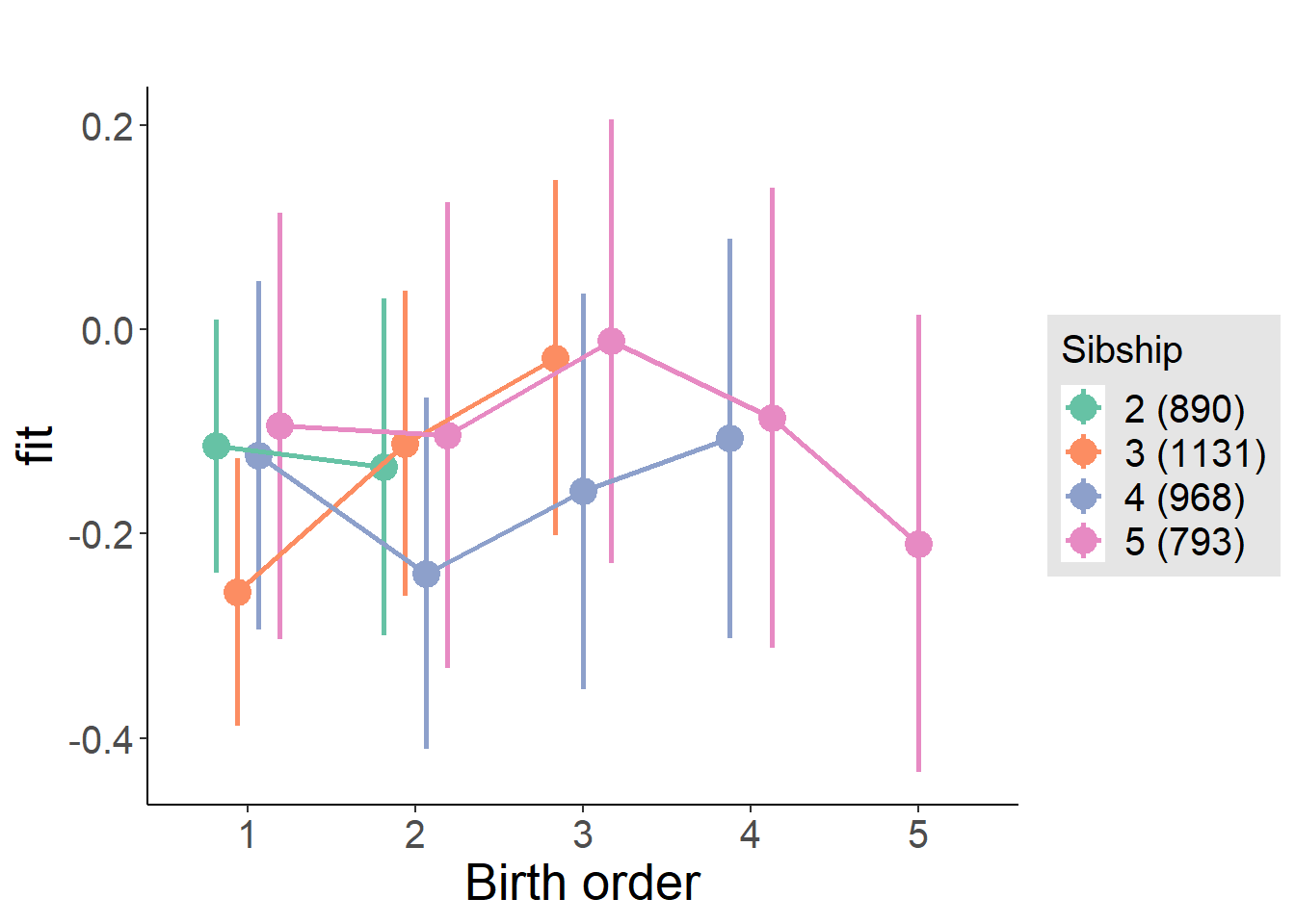
Model Comparison
###### Model 1 - Model 2
anova(m1_covariates_only, m2_birthorder_linear, m3_birthorder_nonlinear, m4_interaction)## refitting model(s) with ML (instead of REML)| Df | AIC | BIC | logLik | deviance | Chisq | Chi Df | Pr(>Chisq) |
|---|---|---|---|---|---|---|---|
| 10 | 10376 | 10439 | -5178 | 10356 | NA | NA | NA |
| 11 | 10377 | 10446 | -5178 | 10355 | 1.043 | 1 | 0.3071 |
| 14 | 10376 | 10463 | -5174 | 10348 | 7.323 | 3 | 0.06229 |
| 20 | 10378 | 10503 | -5169 | 10338 | 9.6 | 6 | 0.1425 |
Parental full sibling order
outcome_parental_m1 <- update(m2_birthorder_linear, data = birthorder %>%
mutate(sibling_count = sibling_count_genes_factor,
birth_order_nonlinear = birthorder_genes_factor,
birth_order = birthorder_genes,
count_birth_order = count_birthorder_genes
) %>%
filter(sibling_count != "1"))
compare_models_markdown(outcome_parental_m1)Basic Model
Model Summary
m1_covariates_only <- update(m2_birthorder_linear, formula = . ~ . - birth_order)
tidy(m1_covariates_only, conf.int = T, conf.level = 0.995)| effect | group | term | estimate | std.error | statistic | df | p.value | conf.low | conf.high |
|---|---|---|---|---|---|---|---|---|---|
| fixed | NA | (Intercept) | 1.817 | 0.5575 | 3.259 | 4050 | 0.001127 | 0.252 | 3.382 |
| fixed | NA | poly(age, 3, raw = TRUE)1 | -0.1648 | 0.06514 | -2.529 | 4048 | 0.01147 | -0.3476 | 0.0181 |
| fixed | NA | poly(age, 3, raw = TRUE)2 | 0.004725 | 0.002404 | 1.966 | 4045 | 0.04942 | -0.002023 | 0.01147 |
| fixed | NA | poly(age, 3, raw = TRUE)3 | -0.00004412 | 0.00002822 | -1.564 | 4041 | 0.118 | -0.0001233 | 0.00003509 |
| fixed | NA | male | -0.26 | 0.02992 | -8.692 | 4019 | 5.093e-18 | -0.344 | -0.1761 |
| fixed | NA | sibling_count3 | -0.01544 | 0.03971 | -0.3887 | 3114 | 0.6975 | -0.1269 | 0.09603 |
| fixed | NA | sibling_count4 | 0.00454 | 0.04313 | 0.1053 | 2735 | 0.9162 | -0.1165 | 0.1256 |
| fixed | NA | sibling_count5 | 0.07114 | 0.05044 | 1.41 | 2338 | 0.1586 | -0.07045 | 0.2127 |
| ran_pars | mother_pidlink | sd__(Intercept) | 0.2604 | NA | NA | NA | NA | NA | NA |
| ran_pars | Residual | sd__Observation | 0.9176 | NA | NA | NA | NA | NA | NA |
Coefficient Plot
plot(allEffects(m1_covariates_only, confidence.level = 0.995))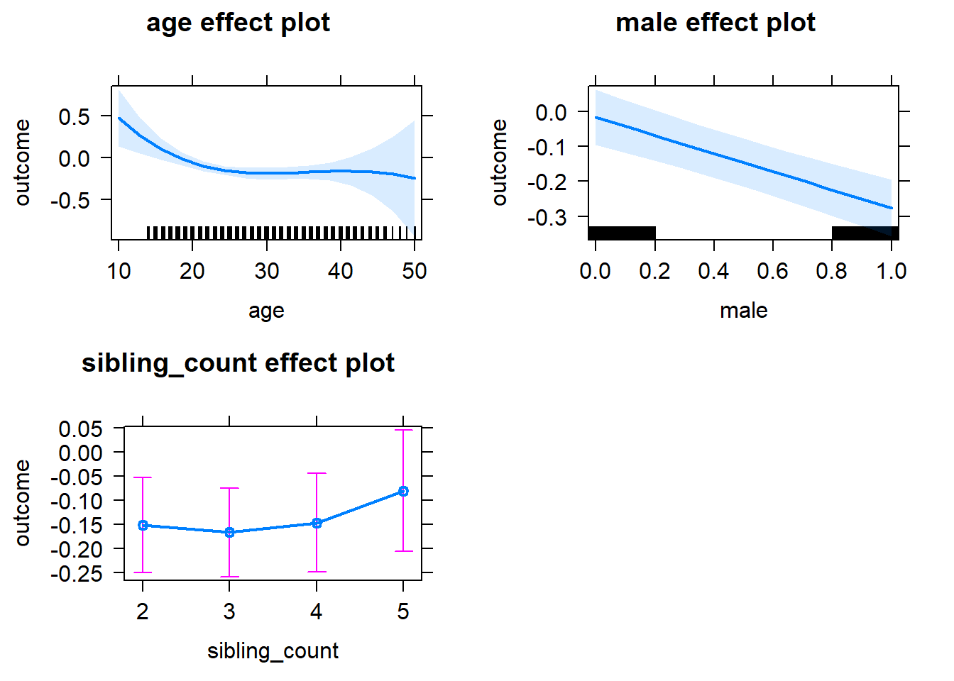
Add Birth Order Linear
Model Summary
tidy(m2_birthorder_linear, conf.int = T, conf.level = 0.995)| effect | group | term | estimate | std.error | statistic | df | p.value | conf.low | conf.high |
|---|---|---|---|---|---|---|---|---|---|
| fixed | NA | (Intercept) | 1.81 | 0.5585 | 3.241 | 4049 | 0.001201 | 0.2424 | 3.378 |
| fixed | NA | birth_order | 0.003336 | 0.01592 | 0.2096 | 3814 | 0.834 | -0.04134 | 0.04801 |
| fixed | NA | poly(age, 3, raw = TRUE)1 | -0.1644 | 0.06517 | -2.523 | 4047 | 0.01167 | -0.3474 | 0.01851 |
| fixed | NA | poly(age, 3, raw = TRUE)2 | 0.004709 | 0.002405 | 1.958 | 4044 | 0.05032 | -0.002043 | 0.01146 |
| fixed | NA | poly(age, 3, raw = TRUE)3 | -0.00004387 | 0.00002825 | -1.553 | 4041 | 0.1205 | -0.0001232 | 0.00003542 |
| fixed | NA | male | -0.2601 | 0.02992 | -8.693 | 4018 | 5.062e-18 | -0.3441 | -0.1761 |
| fixed | NA | sibling_count3 | -0.01704 | 0.04044 | -0.4213 | 3165 | 0.6736 | -0.1306 | 0.09649 |
| fixed | NA | sibling_count4 | 0.0009267 | 0.04645 | 0.01995 | 2968 | 0.9841 | -0.1295 | 0.1313 |
| fixed | NA | sibling_count5 | 0.06544 | 0.0573 | 1.142 | 2766 | 0.2535 | -0.0954 | 0.2263 |
| ran_pars | mother_pidlink | sd__(Intercept) | 0.2604 | NA | NA | NA | NA | NA | NA |
| ran_pars | Residual | sd__Observation | 0.9178 | NA | NA | NA | NA | NA | NA |
Coefficient Plot
plot_birthorder2(m2_birthorder_linear, separate = FALSE)
Add Birth Order Factor
Model Summary
m3_birthorder_nonlinear = update(m1_covariates_only, formula = . ~ . + birth_order_nonlinear)
tidy(m3_birthorder_nonlinear, conf.int = T, conf.level = 0.995)| effect | group | term | estimate | std.error | statistic | df | p.value | conf.low | conf.high |
|---|---|---|---|---|---|---|---|---|---|
| fixed | NA | (Intercept) | 1.785 | 0.559 | 3.194 | 4044 | 0.001416 | 0.2161 | 3.354 |
| fixed | NA | poly(age, 3, raw = TRUE)1 | -0.1612 | 0.06525 | -2.47 | 4042 | 0.01353 | -0.3444 | 0.02196 |
| fixed | NA | poly(age, 3, raw = TRUE)2 | 0.00459 | 0.002408 | 1.906 | 4039 | 0.05674 | -0.00217 | 0.01135 |
| fixed | NA | poly(age, 3, raw = TRUE)3 | -0.00004254 | 0.00002828 | -1.504 | 4036 | 0.1326 | -0.0001219 | 0.00003684 |
| fixed | NA | male | -0.2594 | 0.02993 | -8.668 | 4015 | 6.293e-18 | -0.3435 | -0.1754 |
| fixed | NA | sibling_count3 | -0.02581 | 0.0412 | -0.6265 | 3275 | 0.531 | -0.1415 | 0.08985 |
| fixed | NA | sibling_count4 | -0.008091 | 0.04717 | -0.1715 | 3057 | 0.8638 | -0.1405 | 0.1243 |
| fixed | NA | sibling_count5 | 0.0776 | 0.0585 | 1.327 | 2851 | 0.1848 | -0.08661 | 0.2418 |
| fixed | NA | birth_order_nonlinear2 | 0.008103 | 0.0358 | 0.2263 | 3417 | 0.8209 | -0.09239 | 0.1086 |
| fixed | NA | birth_order_nonlinear3 | 0.0437 | 0.04543 | 0.9619 | 3561 | 0.3362 | -0.08382 | 0.1712 |
| fixed | NA | birth_order_nonlinear4 | 0.01622 | 0.06188 | 0.2621 | 3703 | 0.7933 | -0.1575 | 0.1899 |
| fixed | NA | birth_order_nonlinear5 | -0.08965 | 0.1014 | -0.8839 | 3697 | 0.3768 | -0.3744 | 0.1951 |
| ran_pars | mother_pidlink | sd__(Intercept) | 0.2609 | NA | NA | NA | NA | NA | NA |
| ran_pars | Residual | sd__Observation | 0.9177 | NA | NA | NA | NA | NA | NA |
Coefficient Plot
plot_birthorder(m3_birthorder_nonlinear, separate = FALSE)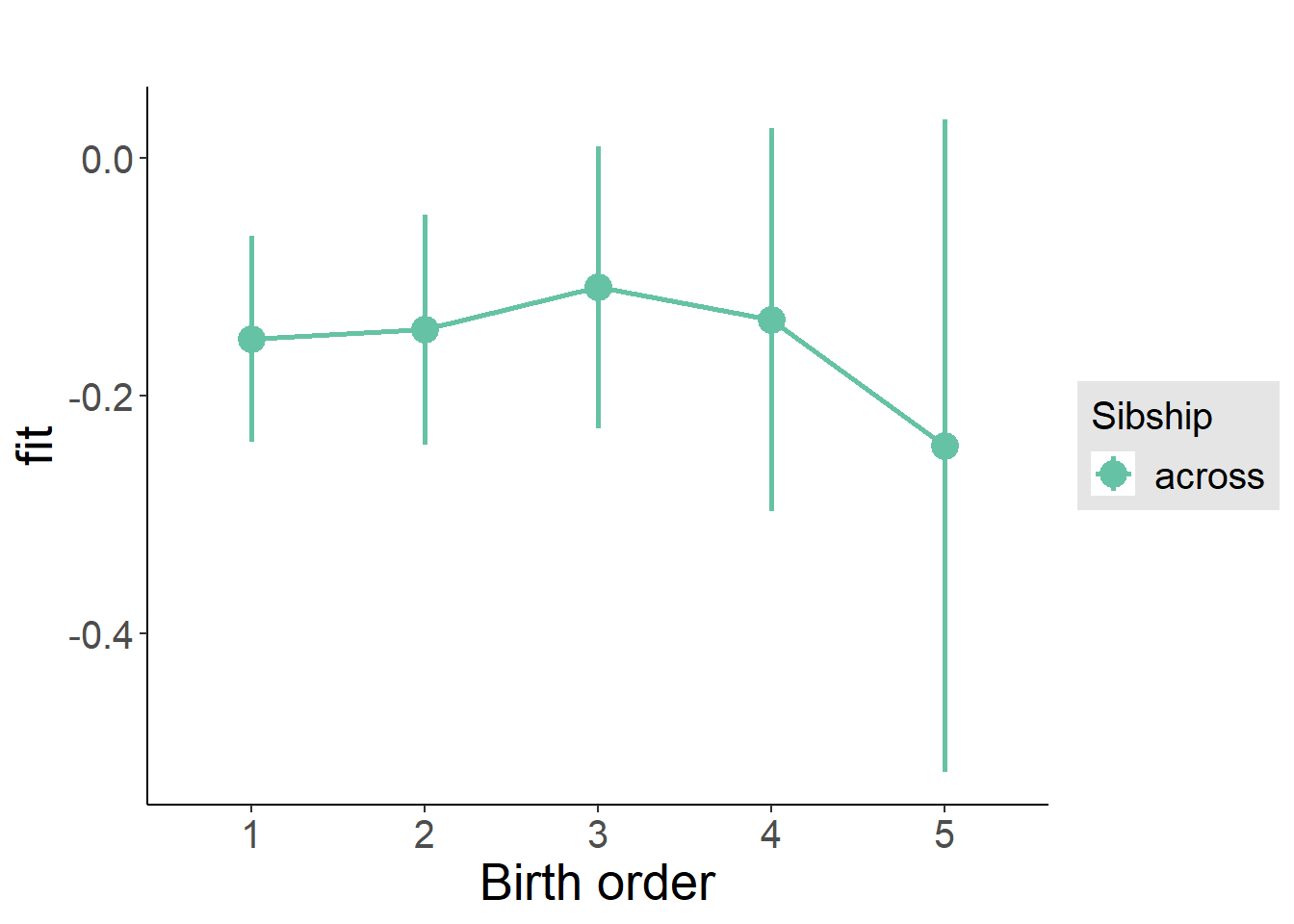
Add Interaction
Model Summary
m4_interaction = update(m3_birthorder_nonlinear, formula = . ~ . - birth_order_nonlinear - sibling_count + count_birth_order)
tidy(m4_interaction, conf.int = T, conf.level = 0.995)| effect | group | term | estimate | std.error | statistic | df | p.value | conf.low | conf.high |
|---|---|---|---|---|---|---|---|---|---|
| fixed | NA | (Intercept) | 1.755 | 0.5588 | 3.14 | 4039 | 0.001701 | 0.1861 | 3.323 |
| fixed | NA | poly(age, 3, raw = TRUE)1 | -0.1567 | 0.06522 | -2.403 | 4037 | 0.01632 | -0.3398 | 0.02637 |
| fixed | NA | poly(age, 3, raw = TRUE)2 | 0.004469 | 0.002407 | 1.857 | 4034 | 0.06344 | -0.002288 | 0.01123 |
| fixed | NA | poly(age, 3, raw = TRUE)3 | -0.0000417 | 0.00002826 | -1.475 | 4031 | 0.1402 | -0.000121 | 0.00003764 |
| fixed | NA | male | -0.2594 | 0.02993 | -8.669 | 4007 | 6.249e-18 | -0.3434 | -0.1754 |
| fixed | NA | count_birth_order2/2 | -0.03975 | 0.05965 | -0.6664 | 3533 | 0.5052 | -0.2072 | 0.1277 |
| fixed | NA | count_birth_order1/3 | -0.1107 | 0.05323 | -2.081 | 4037 | 0.03752 | -0.2602 | 0.03866 |
| fixed | NA | count_birth_order2/3 | -0.00592 | 0.05879 | -0.1007 | 4040 | 0.9198 | -0.171 | 0.1591 |
| fixed | NA | count_birth_order3/3 | 0.09062 | 0.06354 | 1.426 | 4036 | 0.1539 | -0.08773 | 0.269 |
| fixed | NA | count_birth_order1/4 | 0.04216 | 0.06701 | 0.6292 | 4039 | 0.5293 | -0.1459 | 0.2303 |
| fixed | NA | count_birth_order2/4 | 0.006655 | 0.06813 | 0.09768 | 4039 | 0.9222 | -0.1846 | 0.1979 |
| fixed | NA | count_birth_order3/4 | -0.07998 | 0.07193 | -1.112 | 4029 | 0.2662 | -0.2819 | 0.1219 |
| fixed | NA | count_birth_order4/4 | -0.01954 | 0.07381 | -0.2647 | 4028 | 0.7913 | -0.2267 | 0.1877 |
| fixed | NA | count_birth_order1/5 | 0.1313 | 0.09025 | 1.455 | 4040 | 0.1459 | -0.1221 | 0.3846 |
| fixed | NA | count_birth_order2/5 | 0.01481 | 0.09951 | 0.1488 | 4030 | 0.8817 | -0.2645 | 0.2941 |
| fixed | NA | count_birth_order3/5 | 0.05974 | 0.09323 | 0.6407 | 4024 | 0.5217 | -0.202 | 0.3214 |
| fixed | NA | count_birth_order4/5 | 0.09232 | 0.08994 | 1.026 | 4029 | 0.3047 | -0.1601 | 0.3448 |
| fixed | NA | count_birth_order5/5 | -0.029 | 0.09537 | -0.3041 | 4022 | 0.7611 | -0.2967 | 0.2387 |
| ran_pars | mother_pidlink | sd__(Intercept) | 0.2643 | NA | NA | NA | NA | NA | NA |
| ran_pars | Residual | sd__Observation | 0.916 | NA | NA | NA | NA | NA | NA |
Coefficient Plot
plot_birthorder(m4_interaction)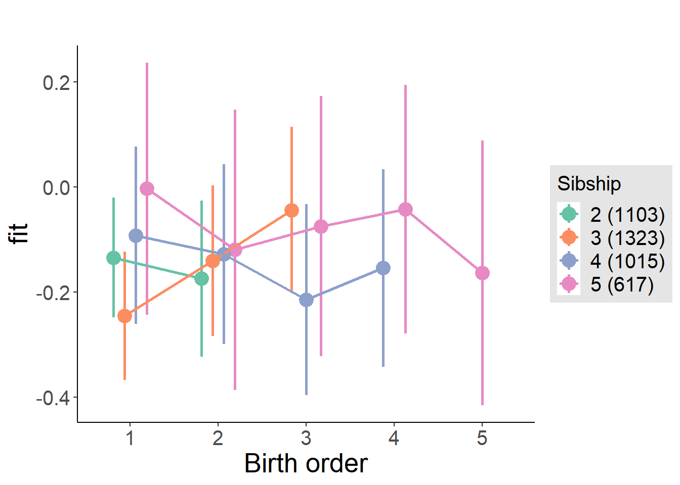
Model Comparison
###### Model 1 - Model 2
anova(m1_covariates_only, m2_birthorder_linear, m3_birthorder_nonlinear, m4_interaction)## refitting model(s) with ML (instead of REML)| Df | AIC | BIC | logLik | deviance | Chisq | Chi Df | Pr(>Chisq) |
|---|---|---|---|---|---|---|---|
| 10 | 11137 | 11200 | -5558 | 11117 | NA | NA | NA |
| 11 | 11139 | 11208 | -5558 | 11117 | 0.04383 | 1 | 0.8342 |
| 14 | 11142 | 11231 | -5557 | 11114 | 2.104 | 3 | 0.5512 |
| 20 | 11142 | 11268 | -5551 | 11102 | 12.71 | 6 | 0.04789 |
Compare birth order specifications
library(coefplot)
multiplot(outcome_naive_m1, outcome_preg_m1, outcome_uterus_m1, outcome_parental_m1, dodgeHeight = 0.6,
intercept = FALSE)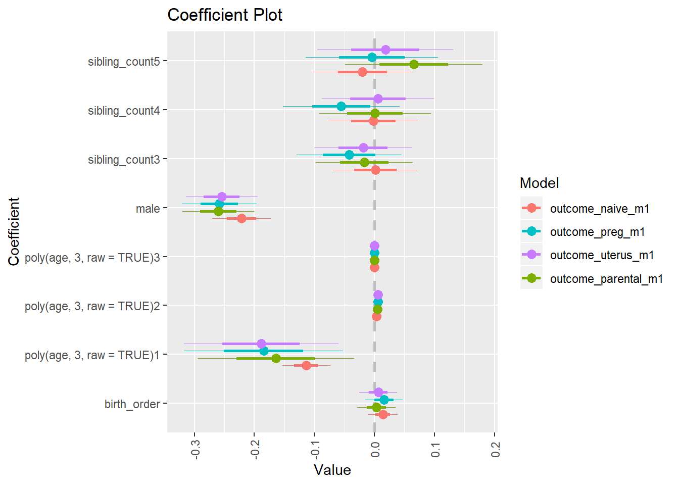
Risk B
birthorder <- birthorder %>% mutate(outcome = riskB)
model = lmer(outcome ~ birth_order + poly(age, 3, raw = TRUE) + male + sibling_count + (1 | mother_pidlink),
data = birthorder)
compare_birthorder_specs(model)Naive birth order
outcome_naive_m1 <- update(m2_birthorder_linear, data = birthorder %>%
mutate(sibling_count = sibling_count_naive_factor,
birth_order_nonlinear = birthorder_naive_factor,
birth_order = birthorder_naive,
count_birth_order = count_birthorder_naive) %>%
filter(sibling_count != "1"))
compare_models_markdown(outcome_naive_m1)Basic Model
Model Summary
m1_covariates_only <- update(m2_birthorder_linear, formula = . ~ . - birth_order)
tidy(m1_covariates_only, conf.int = T, conf.level = 0.995)| effect | group | term | estimate | std.error | statistic | df | p.value | conf.low | conf.high |
|---|---|---|---|---|---|---|---|---|---|
| fixed | NA | (Intercept) | 0.6854 | 0.2014 | 3.404 | 6324 | 0.000669 | 0.1202 | 1.251 |
| fixed | NA | poly(age, 3, raw = TRUE)1 | -0.0475 | 0.0193 | -2.461 | 6130 | 0.01387 | -0.1017 | 0.006673 |
| fixed | NA | poly(age, 3, raw = TRUE)2 | 0.001242 | 0.0005621 | 2.209 | 5915 | 0.02721 | -0.0003361 | 0.00282 |
| fixed | NA | poly(age, 3, raw = TRUE)3 | -0.00001056 | 0.000005087 | -2.075 | 5744 | 0.03804 | -0.00002484 | 0.000003725 |
| fixed | NA | male | -0.2056 | 0.02369 | -8.679 | 6732 | 4.944e-18 | -0.2721 | -0.1391 |
| fixed | NA | sibling_count3 | -0.02283 | 0.03353 | -0.6809 | 4779 | 0.4959 | -0.117 | 0.07129 |
| fixed | NA | sibling_count4 | -0.005103 | 0.03461 | -0.1474 | 4283 | 0.8828 | -0.1023 | 0.09206 |
| fixed | NA | sibling_count5 | -0.02601 | 0.03576 | -0.7275 | 3635 | 0.467 | -0.1264 | 0.07436 |
| ran_pars | mother_pidlink | sd__(Intercept) | 0.2471 | NA | NA | NA | NA | NA | NA |
| ran_pars | Residual | sd__Observation | 0.9435 | NA | NA | NA | NA | NA | NA |
Coefficient Plot
plot(allEffects(m1_covariates_only, confidence.level = 0.995))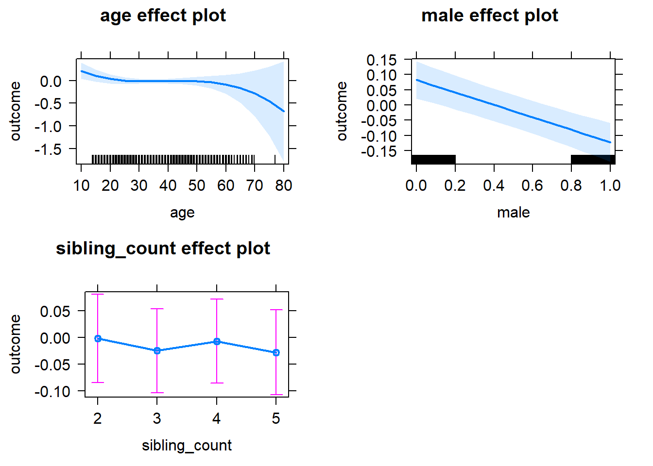
Add Birth Order Linear
Model Summary
tidy(m2_birthorder_linear, conf.int = T, conf.level = 0.995)| effect | group | term | estimate | std.error | statistic | df | p.value | conf.low | conf.high |
|---|---|---|---|---|---|---|---|---|---|
| fixed | NA | (Intercept) | 0.6772 | 0.2014 | 3.362 | 6314 | 0.0007772 | 0.1119 | 1.243 |
| fixed | NA | birth_order | 0.02396 | 0.01188 | 2.017 | 5870 | 0.04378 | -0.009391 | 0.05731 |
| fixed | NA | poly(age, 3, raw = TRUE)1 | -0.04989 | 0.01933 | -2.581 | 6157 | 0.009878 | -0.1042 | 0.004372 |
| fixed | NA | poly(age, 3, raw = TRUE)2 | 0.001303 | 0.0005629 | 2.314 | 5930 | 0.02068 | -0.0002773 | 0.002883 |
| fixed | NA | poly(age, 3, raw = TRUE)3 | -0.00001096 | 0.000005091 | -2.152 | 5752 | 0.03143 | -0.00002525 | 0.000003334 |
| fixed | NA | male | -0.2063 | 0.02368 | -8.709 | 6729 | 3.796e-18 | -0.2727 | -0.1398 |
| fixed | NA | sibling_count3 | -0.03147 | 0.0338 | -0.9311 | 4901 | 0.3518 | -0.1264 | 0.06341 |
| fixed | NA | sibling_count4 | -0.02493 | 0.03598 | -0.6929 | 4801 | 0.4884 | -0.1259 | 0.07607 |
| fixed | NA | sibling_count5 | -0.05847 | 0.03921 | -1.491 | 4715 | 0.136 | -0.1685 | 0.0516 |
| ran_pars | mother_pidlink | sd__(Intercept) | 0.2482 | NA | NA | NA | NA | NA | NA |
| ran_pars | Residual | sd__Observation | 0.943 | NA | NA | NA | NA | NA | NA |
Coefficient Plot
plot_birthorder2(m2_birthorder_linear, separate = FALSE)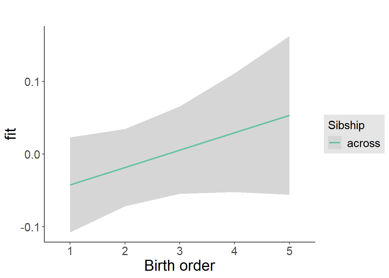
Add Birth Order Factor
Model Summary
m3_birthorder_nonlinear = update(m1_covariates_only, formula = . ~ . + birth_order_nonlinear)
tidy(m3_birthorder_nonlinear, conf.int = T, conf.level = 0.995)| effect | group | term | estimate | std.error | statistic | df | p.value | conf.low | conf.high |
|---|---|---|---|---|---|---|---|---|---|
| fixed | NA | (Intercept) | 0.7023 | 0.202 | 3.476 | 6338 | 0.0005126 | 0.1351 | 1.269 |
| fixed | NA | poly(age, 3, raw = TRUE)1 | -0.04983 | 0.01934 | -2.576 | 6144 | 0.01002 | -0.1041 | 0.004473 |
| fixed | NA | poly(age, 3, raw = TRUE)2 | 0.001303 | 0.0005634 | 2.312 | 5907 | 0.0208 | -0.0002788 | 0.002884 |
| fixed | NA | poly(age, 3, raw = TRUE)3 | -0.00001097 | 0.000005097 | -2.153 | 5719 | 0.03139 | -0.00002528 | 0.000003336 |
| fixed | NA | male | -0.2063 | 0.02369 | -8.708 | 6727 | 3.836e-18 | -0.2728 | -0.1398 |
| fixed | NA | sibling_count3 | -0.03303 | 0.03436 | -0.9614 | 5111 | 0.3364 | -0.1295 | 0.06342 |
| fixed | NA | sibling_count4 | -0.02257 | 0.0366 | -0.6166 | 5031 | 0.5375 | -0.1253 | 0.08017 |
| fixed | NA | sibling_count5 | -0.06135 | 0.03959 | -1.55 | 4884 | 0.1213 | -0.1725 | 0.04979 |
| fixed | NA | birth_order_nonlinear2 | 0.01745 | 0.0282 | 0.619 | 5718 | 0.536 | -0.0617 | 0.09661 |
| fixed | NA | birth_order_nonlinear3 | 0.05327 | 0.03634 | 1.466 | 5738 | 0.1427 | -0.04873 | 0.1553 |
| fixed | NA | birth_order_nonlinear4 | 0.04952 | 0.04752 | 1.042 | 5782 | 0.2975 | -0.08388 | 0.1829 |
| fixed | NA | birth_order_nonlinear5 | 0.1235 | 0.06842 | 1.806 | 5632 | 0.07105 | -0.06852 | 0.3156 |
| ran_pars | mother_pidlink | sd__(Intercept) | 0.2471 | NA | NA | NA | NA | NA | NA |
| ran_pars | Residual | sd__Observation | 0.9434 | NA | NA | NA | NA | NA | NA |
Coefficient Plot
plot_birthorder(m3_birthorder_nonlinear, separate = FALSE)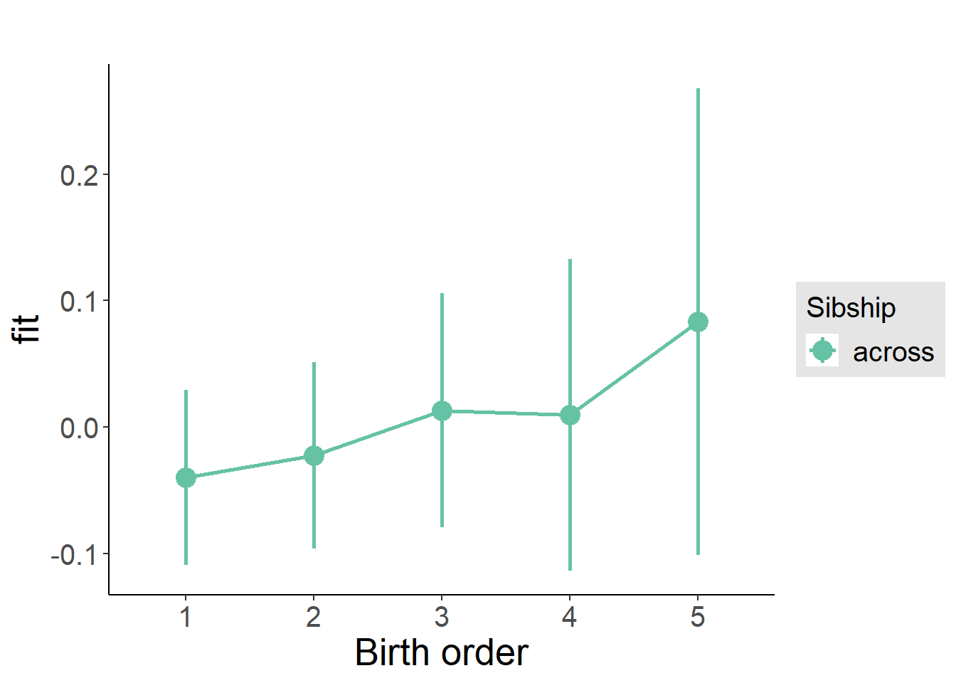
Add Interaction
Model Summary
m4_interaction = update(m3_birthorder_nonlinear, formula = . ~ . - birth_order_nonlinear - sibling_count + count_birth_order)
tidy(m4_interaction, conf.int = T, conf.level = 0.995)| effect | group | term | estimate | std.error | statistic | df | p.value | conf.low | conf.high |
|---|---|---|---|---|---|---|---|---|---|
| fixed | NA | (Intercept) | 0.7358 | 0.2022 | 3.638 | 6344 | 0.0002767 | 0.1681 | 1.304 |
| fixed | NA | poly(age, 3, raw = TRUE)1 | -0.05063 | 0.01933 | -2.62 | 6144 | 0.008827 | -0.1049 | 0.003624 |
| fixed | NA | poly(age, 3, raw = TRUE)2 | 0.001323 | 0.0005628 | 2.35 | 5905 | 0.01879 | -0.000257 | 0.002903 |
| fixed | NA | poly(age, 3, raw = TRUE)3 | -0.00001111 | 0.000005091 | -2.181 | 5713 | 0.02919 | -0.0000254 | 0.000003185 |
| fixed | NA | male | -0.2065 | 0.02367 | -8.726 | 6720 | 3.292e-18 | -0.2729 | -0.1401 |
| fixed | NA | count_birth_order2/2 | -0.04957 | 0.04813 | -1.03 | 5643 | 0.3031 | -0.1847 | 0.08554 |
| fixed | NA | count_birth_order1/3 | -0.1253 | 0.04511 | -2.778 | 6752 | 0.005484 | -0.252 | 0.001307 |
| fixed | NA | count_birth_order2/3 | 0.002572 | 0.05029 | 0.05114 | 6759 | 0.9592 | -0.1386 | 0.1437 |
| fixed | NA | count_birth_order3/3 | 0.07243 | 0.05665 | 1.278 | 6761 | 0.2011 | -0.08659 | 0.2314 |
| fixed | NA | count_birth_order1/4 | 0.03681 | 0.05155 | 0.7141 | 6759 | 0.4752 | -0.1079 | 0.1815 |
| fixed | NA | count_birth_order2/4 | -0.03557 | 0.05444 | -0.6534 | 6761 | 0.5135 | -0.1884 | 0.1172 |
| fixed | NA | count_birth_order3/4 | -0.1211 | 0.05978 | -2.025 | 6760 | 0.04289 | -0.2889 | 0.04674 |
| fixed | NA | count_birth_order4/4 | 0.007753 | 0.06279 | 0.1235 | 6758 | 0.9017 | -0.1685 | 0.184 |
| fixed | NA | count_birth_order1/5 | -0.13 | 0.05888 | -2.209 | 6760 | 0.02724 | -0.2953 | 0.03524 |
| fixed | NA | count_birth_order2/5 | -0.05497 | 0.06115 | -0.899 | 6758 | 0.3687 | -0.2266 | 0.1167 |
| fixed | NA | count_birth_order3/5 | 0.0107 | 0.06276 | 0.1705 | 6757 | 0.8646 | -0.1655 | 0.1869 |
| fixed | NA | count_birth_order4/5 | -0.04345 | 0.06722 | -0.6464 | 6751 | 0.5181 | -0.2322 | 0.1453 |
| fixed | NA | count_birth_order5/5 | 0.038 | 0.06807 | 0.5582 | 6751 | 0.5767 | -0.1531 | 0.2291 |
| ran_pars | mother_pidlink | sd__(Intercept) | 0.2474 | NA | NA | NA | NA | NA | NA |
| ran_pars | Residual | sd__Observation | 0.9422 | NA | NA | NA | NA | NA | NA |
Coefficient Plot
plot_birthorder(m4_interaction)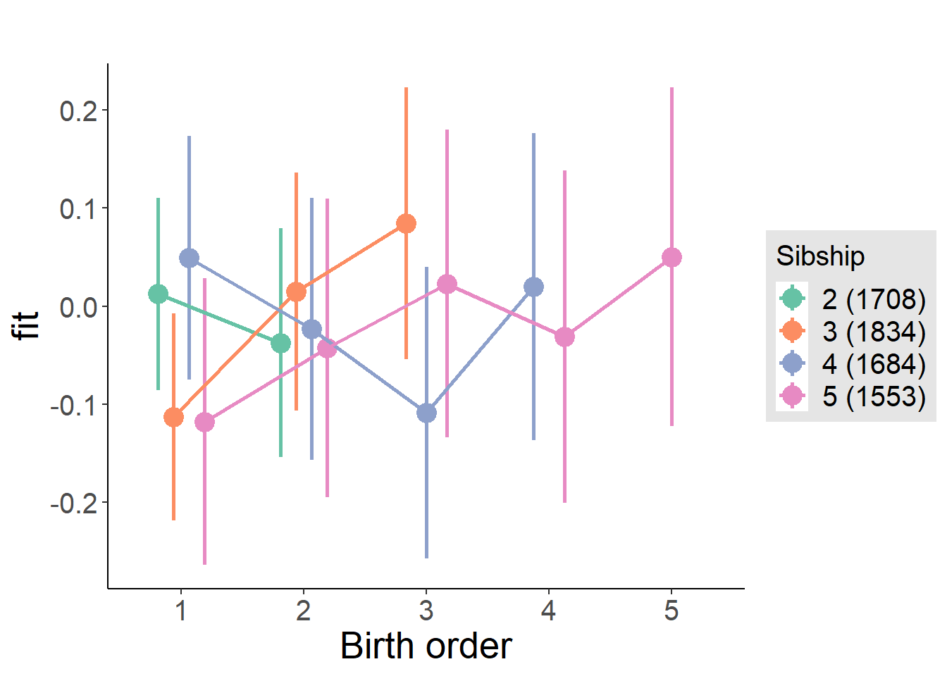
Model Comparison
###### Model 1 - Model 2
anova(m1_covariates_only, m2_birthorder_linear, m3_birthorder_nonlinear, m4_interaction)## refitting model(s) with ML (instead of REML)| Df | AIC | BIC | logLik | deviance | Chisq | Chi Df | Pr(>Chisq) |
|---|---|---|---|---|---|---|---|
| 10 | 18899 | 18967 | -9439 | 18879 | NA | NA | NA |
| 11 | 18897 | 18972 | -9437 | 18875 | 4.067 | 1 | 0.04373 |
| 14 | 18902 | 18998 | -9437 | 18874 | 0.6018 | 3 | 0.896 |
| 20 | 18892 | 19029 | -9426 | 18852 | 21.85 | 6 | 0.001288 |
Maternal birth order
outcome_uterus_m1 <- update(m2_birthorder_linear, data = birthorder %>%
mutate(sibling_count = sibling_count_uterus_alive_factor,
birth_order_nonlinear = birthorder_uterus_alive_factor,
birth_order = birthorder_uterus_alive,
count_birth_order = count_birthorder_uterus_alive) %>%
filter(sibling_count != "1"))
compare_models_markdown(outcome_uterus_m1)Basic Model
Model Summary
m1_covariates_only <- update(m2_birthorder_linear, formula = . ~ . - birth_order)
tidy(m1_covariates_only, conf.int = T, conf.level = 0.995)| effect | group | term | estimate | std.error | statistic | df | p.value | conf.low | conf.high |
|---|---|---|---|---|---|---|---|---|---|
| fixed | NA | (Intercept) | 1.277 | 0.5329 | 2.397 | 4261 | 0.01658 | -0.2186 | 2.773 |
| fixed | NA | poly(age, 3, raw = TRUE)1 | -0.113 | 0.06212 | -1.819 | 4256 | 0.06901 | -0.2874 | 0.06139 |
| fixed | NA | poly(age, 3, raw = TRUE)2 | 0.003652 | 0.002288 | 1.596 | 4249 | 0.1106 | -0.002771 | 0.01007 |
| fixed | NA | poly(age, 3, raw = TRUE)3 | -0.00003752 | 0.0000268 | -1.4 | 4244 | 0.1617 | -0.0001128 | 0.00003772 |
| fixed | NA | male | -0.2354 | 0.02876 | -8.183 | 4262 | 3.623e-16 | -0.3161 | -0.1546 |
| fixed | NA | sibling_count3 | -0.07681 | 0.03814 | -2.014 | 3189 | 0.04413 | -0.1839 | 0.03026 |
| fixed | NA | sibling_count4 | -0.0239 | 0.04097 | -0.5835 | 2703 | 0.5596 | -0.1389 | 0.09109 |
| fixed | NA | sibling_count5 | -0.05159 | 0.04645 | -1.11 | 2289 | 0.2669 | -0.182 | 0.07881 |
| ran_pars | mother_pidlink | sd__(Intercept) | 0.1342 | NA | NA | NA | NA | NA | NA |
| ran_pars | Residual | sd__Observation | 0.9283 | NA | NA | NA | NA | NA | NA |
Coefficient Plot
plot(allEffects(m1_covariates_only, confidence.level = 0.995))
Add Birth Order Linear
Model Summary
tidy(m2_birthorder_linear, conf.int = T, conf.level = 0.995)| effect | group | term | estimate | std.error | statistic | df | p.value | conf.low | conf.high |
|---|---|---|---|---|---|---|---|---|---|
| fixed | NA | (Intercept) | 1.262 | 0.5335 | 2.367 | 4260 | 0.018 | -0.235 | 2.76 |
| fixed | NA | birth_order | 0.009315 | 0.01523 | 0.6117 | 4054 | 0.5408 | -0.03343 | 0.05206 |
| fixed | NA | poly(age, 3, raw = TRUE)1 | -0.1125 | 0.06213 | -1.811 | 4255 | 0.07021 | -0.2869 | 0.06189 |
| fixed | NA | poly(age, 3, raw = TRUE)2 | 0.003624 | 0.002289 | 1.583 | 4249 | 0.1134 | -0.002801 | 0.01005 |
| fixed | NA | poly(age, 3, raw = TRUE)3 | -0.00003701 | 0.00002682 | -1.38 | 4244 | 0.1676 | -0.0001123 | 0.00003827 |
| fixed | NA | male | -0.2357 | 0.02877 | -8.193 | 4261 | 3.338e-16 | -0.3165 | -0.155 |
| fixed | NA | sibling_count3 | -0.08109 | 0.03879 | -2.09 | 3247 | 0.03666 | -0.19 | 0.0278 |
| fixed | NA | sibling_count4 | -0.03366 | 0.04399 | -0.7652 | 2942 | 0.4442 | -0.1572 | 0.08983 |
| fixed | NA | sibling_count5 | -0.06788 | 0.05358 | -1.267 | 2819 | 0.2053 | -0.2183 | 0.08253 |
| ran_pars | mother_pidlink | sd__(Intercept) | 0.1366 | NA | NA | NA | NA | NA | NA |
| ran_pars | Residual | sd__Observation | 0.9281 | NA | NA | NA | NA | NA | NA |
Coefficient Plot
plot_birthorder2(m2_birthorder_linear, separate = FALSE)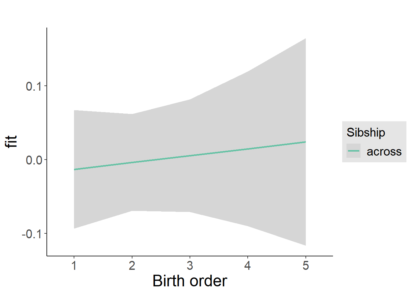
Add Birth Order Factor
Model Summary
m3_birthorder_nonlinear = update(m1_covariates_only, formula = . ~ . + birth_order_nonlinear)
tidy(m3_birthorder_nonlinear, conf.int = T, conf.level = 0.995)| effect | group | term | estimate | std.error | statistic | df | p.value | conf.low | conf.high |
|---|---|---|---|---|---|---|---|---|---|
| fixed | NA | (Intercept) | 1.239 | 0.5338 | 2.32 | 4254 | 0.02037 | -0.2598 | 2.737 |
| fixed | NA | poly(age, 3, raw = TRUE)1 | -0.1096 | 0.06218 | -1.763 | 4249 | 0.07796 | -0.2842 | 0.06491 |
| fixed | NA | poly(age, 3, raw = TRUE)2 | 0.003517 | 0.00229 | 1.536 | 4243 | 0.1247 | -0.002912 | 0.009946 |
| fixed | NA | poly(age, 3, raw = TRUE)3 | -0.00003582 | 0.00002683 | -1.335 | 4238 | 0.1819 | -0.0001111 | 0.0000395 |
| fixed | NA | male | -0.2352 | 0.02878 | -8.172 | 4258 | 3.952e-16 | -0.316 | -0.1544 |
| fixed | NA | sibling_count3 | -0.08894 | 0.03946 | -2.254 | 3370 | 0.02427 | -0.1997 | 0.02183 |
| fixed | NA | sibling_count4 | -0.04037 | 0.04471 | -0.9029 | 3045 | 0.3666 | -0.1659 | 0.08513 |
| fixed | NA | sibling_count5 | -0.05315 | 0.0545 | -0.9753 | 2892 | 0.3295 | -0.2061 | 0.09983 |
| fixed | NA | birth_order_nonlinear2 | 0.03623 | 0.03476 | 1.042 | 3565 | 0.2973 | -0.06134 | 0.1338 |
| fixed | NA | birth_order_nonlinear3 | 0.05454 | 0.04425 | 1.232 | 3800 | 0.2178 | -0.06968 | 0.1788 |
| fixed | NA | birth_order_nonlinear4 | 0.0318 | 0.05894 | 0.5394 | 3980 | 0.5896 | -0.1337 | 0.1973 |
| fixed | NA | birth_order_nonlinear5 | -0.05454 | 0.09276 | -0.5879 | 3908 | 0.5566 | -0.3149 | 0.2058 |
| ran_pars | mother_pidlink | sd__(Intercept) | 0.1319 | NA | NA | NA | NA | NA | NA |
| ran_pars | Residual | sd__Observation | 0.9288 | NA | NA | NA | NA | NA | NA |
Coefficient Plot
plot_birthorder(m3_birthorder_nonlinear, separate = FALSE)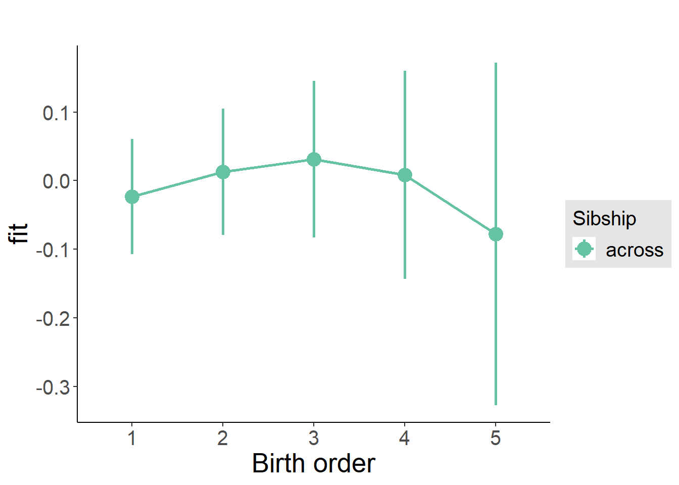
Add Interaction
Model Summary
m4_interaction = update(m3_birthorder_nonlinear, formula = . ~ . - birth_order_nonlinear - sibling_count + count_birth_order)
tidy(m4_interaction, conf.int = T, conf.level = 0.995)| effect | group | term | estimate | std.error | statistic | df | p.value | conf.low | conf.high |
|---|---|---|---|---|---|---|---|---|---|
| fixed | NA | (Intercept) | 1.208 | 0.5335 | 2.265 | 4249 | 0.02358 | -0.2893 | 2.706 |
| fixed | NA | poly(age, 3, raw = TRUE)1 | -0.1068 | 0.06215 | -1.719 | 4244 | 0.08568 | -0.2813 | 0.06762 |
| fixed | NA | poly(age, 3, raw = TRUE)2 | 0.003458 | 0.002289 | 1.511 | 4238 | 0.1309 | -0.002968 | 0.009885 |
| fixed | NA | poly(age, 3, raw = TRUE)3 | -0.00003564 | 0.00002682 | -1.329 | 4233 | 0.184 | -0.0001109 | 0.00003966 |
| fixed | NA | male | -0.2341 | 0.02877 | -8.139 | 4252 | 5.195e-16 | -0.3149 | -0.1534 |
| fixed | NA | count_birth_order2/2 | 0.02688 | 0.05921 | 0.4541 | 3652 | 0.6498 | -0.1393 | 0.1931 |
| fixed | NA | count_birth_order1/3 | -0.1468 | 0.0516 | -2.844 | 4254 | 0.00447 | -0.2916 | -0.001931 |
| fixed | NA | count_birth_order2/3 | -0.006226 | 0.05624 | -0.1107 | 4254 | 0.9119 | -0.1641 | 0.1516 |
| fixed | NA | count_birth_order3/3 | -0.003739 | 0.06312 | -0.05924 | 4253 | 0.9528 | -0.1809 | 0.1734 |
| fixed | NA | count_birth_order1/4 | 0.01079 | 0.06345 | 0.17 | 4252 | 0.865 | -0.1673 | 0.1889 |
| fixed | NA | count_birth_order2/4 | -0.02773 | 0.06572 | -0.4219 | 4254 | 0.6731 | -0.2122 | 0.1568 |
| fixed | NA | count_birth_order3/4 | -0.07186 | 0.0693 | -1.037 | 4252 | 0.2998 | -0.2664 | 0.1227 |
| fixed | NA | count_birth_order4/4 | 0.02637 | 0.07157 | 0.3684 | 4251 | 0.7126 | -0.1745 | 0.2273 |
| fixed | NA | count_birth_order1/5 | 0.03834 | 0.08726 | 0.4393 | 4254 | 0.6605 | -0.2066 | 0.2833 |
| fixed | NA | count_birth_order2/5 | -0.1342 | 0.09153 | -1.467 | 4254 | 0.1426 | -0.3912 | 0.1227 |
| fixed | NA | count_birth_order3/5 | 0.06427 | 0.08583 | 0.7488 | 4252 | 0.454 | -0.1766 | 0.3052 |
| fixed | NA | count_birth_order4/5 | -0.08061 | 0.08253 | -0.9768 | 4251 | 0.3287 | -0.3123 | 0.1511 |
| fixed | NA | count_birth_order5/5 | -0.1119 | 0.08703 | -1.286 | 4248 | 0.1986 | -0.3562 | 0.1324 |
| ran_pars | mother_pidlink | sd__(Intercept) | 0.1324 | NA | NA | NA | NA | NA | NA |
| ran_pars | Residual | sd__Observation | 0.928 | NA | NA | NA | NA | NA | NA |
Coefficient Plot
plot_birthorder(m4_interaction)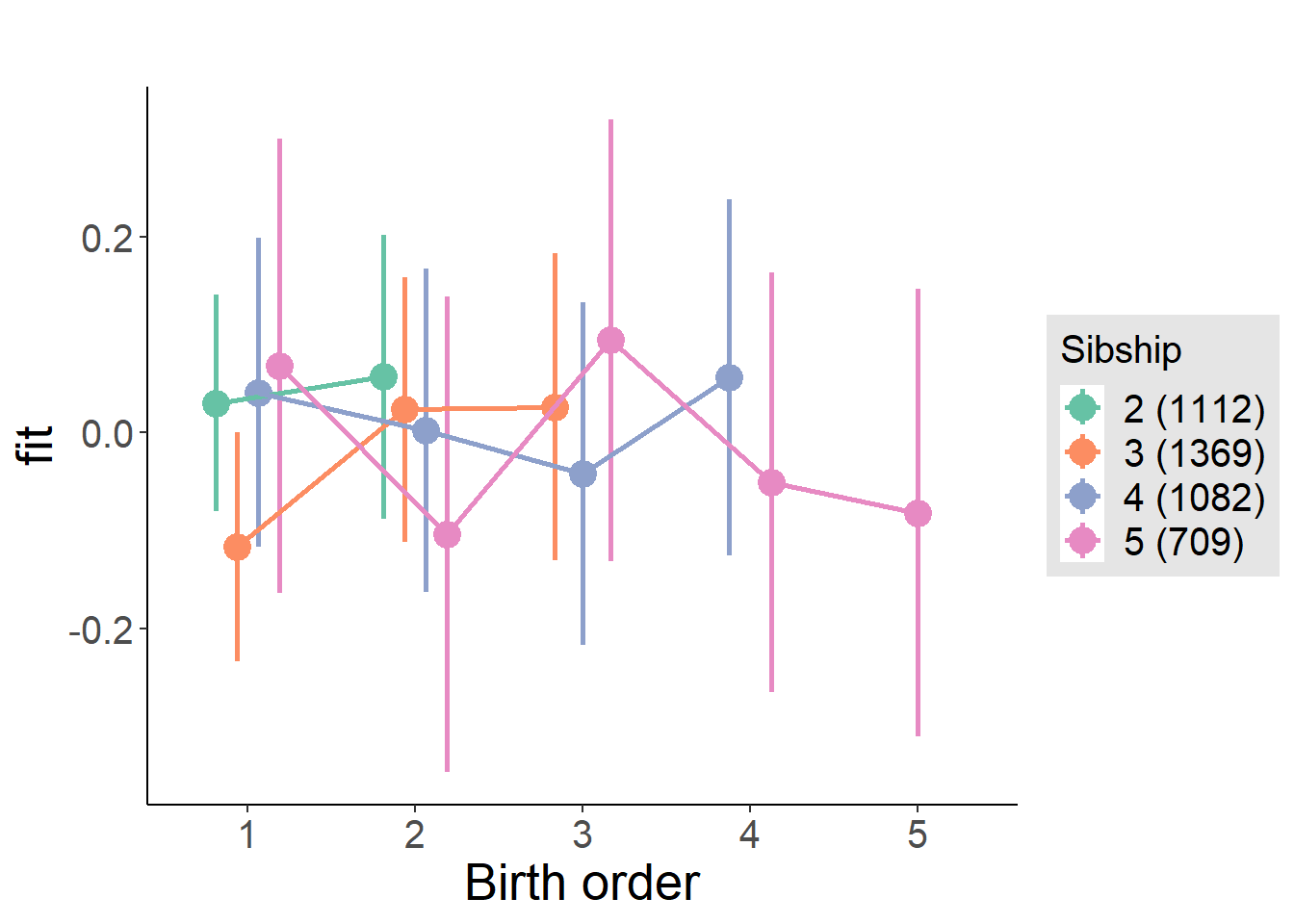
Model Comparison
###### Model 1 - Model 2
anova(m1_covariates_only, m2_birthorder_linear, m3_birthorder_nonlinear, m4_interaction)## refitting model(s) with ML (instead of REML)| Df | AIC | BIC | logLik | deviance | Chisq | Chi Df | Pr(>Chisq) |
|---|---|---|---|---|---|---|---|
| 10 | 11588 | 11651 | -5784 | 11568 | NA | NA | NA |
| 11 | 11589 | 11659 | -5784 | 11567 | 0.3712 | 1 | 0.5423 |
| 14 | 11593 | 11682 | -5782 | 11565 | 2.509 | 3 | 0.4737 |
| 20 | 11593 | 11720 | -5776 | 11553 | 11.94 | 6 | 0.06337 |
Maternal pregnancy order
outcome_preg_m1 <- update(m2_birthorder_linear, data = birthorder %>%
mutate(sibling_count = sibling_count_uterus_preg_factor,
birth_order_nonlinear = birthorder_uterus_preg_factor,
birth_order = birthorder_uterus_preg,
count_birth_order = count_birthorder_uterus_preg
) %>%
filter(sibling_count != "1"))
compare_models_markdown(outcome_preg_m1)Basic Model
Model Summary
m1_covariates_only <- update(m2_birthorder_linear, formula = . ~ . - birth_order)
tidy(m1_covariates_only, conf.int = T, conf.level = 0.995)| effect | group | term | estimate | std.error | statistic | df | p.value | conf.low | conf.high |
|---|---|---|---|---|---|---|---|---|---|
| fixed | NA | (Intercept) | 1.164 | 0.5493 | 2.12 | 3962 | 0.0341 | -0.3776 | 2.706 |
| fixed | NA | poly(age, 3, raw = TRUE)1 | -0.09927 | 0.06411 | -1.549 | 3958 | 0.1216 | -0.2792 | 0.08068 |
| fixed | NA | poly(age, 3, raw = TRUE)2 | 0.003195 | 0.002362 | 1.353 | 3953 | 0.1763 | -0.003436 | 0.009825 |
| fixed | NA | poly(age, 3, raw = TRUE)3 | -0.00003294 | 0.00002767 | -1.191 | 3949 | 0.2339 | -0.0001106 | 0.00004473 |
| fixed | NA | male | -0.2337 | 0.02989 | -7.819 | 3960 | 6.782e-15 | -0.3176 | -0.1498 |
| fixed | NA | sibling_count3 | -0.09083 | 0.04143 | -2.192 | 3035 | 0.02844 | -0.2071 | 0.02547 |
| fixed | NA | sibling_count4 | -0.04567 | 0.04367 | -1.046 | 2694 | 0.2957 | -0.1683 | 0.07691 |
| fixed | NA | sibling_count5 | -0.0509 | 0.04655 | -1.093 | 2324 | 0.2743 | -0.1816 | 0.07977 |
| ran_pars | mother_pidlink | sd__(Intercept) | 0.1607 | NA | NA | NA | NA | NA | NA |
| ran_pars | Residual | sd__Observation | 0.9259 | NA | NA | NA | NA | NA | NA |
Coefficient Plot
plot(allEffects(m1_covariates_only, confidence.level = 0.995))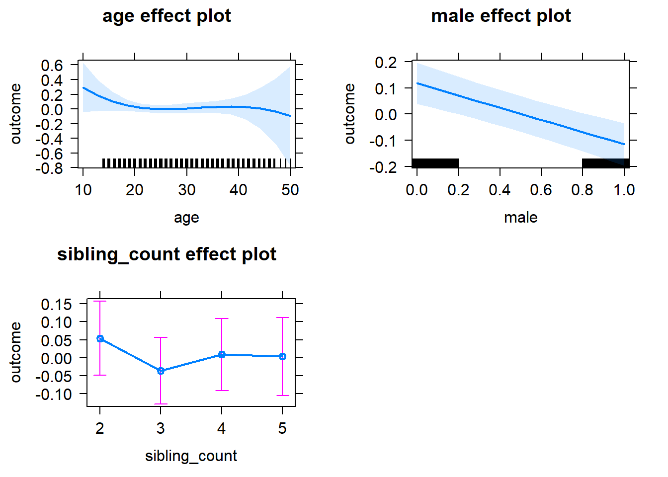
Add Birth Order Linear
Model Summary
tidy(m2_birthorder_linear, conf.int = T, conf.level = 0.995)| effect | group | term | estimate | std.error | statistic | df | p.value | conf.low | conf.high |
|---|---|---|---|---|---|---|---|---|---|
| fixed | NA | (Intercept) | 1.149 | 0.5499 | 2.089 | 3961 | 0.03679 | -0.395 | 2.692 |
| fixed | NA | birth_order | 0.009936 | 0.01523 | 0.6523 | 3815 | 0.5143 | -0.03282 | 0.0527 |
| fixed | NA | poly(age, 3, raw = TRUE)1 | -0.09881 | 0.06411 | -1.541 | 3958 | 0.1234 | -0.2788 | 0.08117 |
| fixed | NA | poly(age, 3, raw = TRUE)2 | 0.003167 | 0.002363 | 1.34 | 3953 | 0.1802 | -0.003465 | 0.009799 |
| fixed | NA | poly(age, 3, raw = TRUE)3 | -0.00003242 | 0.00002769 | -1.171 | 3949 | 0.2416 | -0.0001101 | 0.00004529 |
| fixed | NA | male | -0.2339 | 0.02989 | -7.824 | 3959 | 6.509e-15 | -0.3178 | -0.15 |
| fixed | NA | sibling_count3 | -0.09537 | 0.04202 | -2.269 | 3074 | 0.02331 | -0.2133 | 0.02259 |
| fixed | NA | sibling_count4 | -0.05566 | 0.0463 | -1.202 | 2859 | 0.2295 | -0.1856 | 0.07432 |
| fixed | NA | sibling_count5 | -0.06693 | 0.05269 | -1.27 | 2739 | 0.2041 | -0.2148 | 0.08096 |
| ran_pars | mother_pidlink | sd__(Intercept) | 0.1628 | NA | NA | NA | NA | NA | NA |
| ran_pars | Residual | sd__Observation | 0.9256 | NA | NA | NA | NA | NA | NA |
Coefficient Plot
plot_birthorder2(m2_birthorder_linear, separate = FALSE)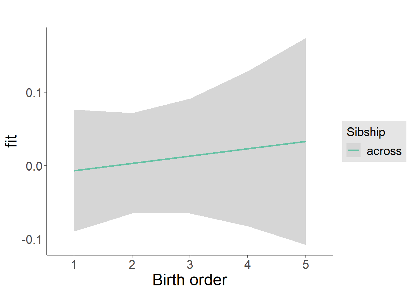
Add Birth Order Factor
Model Summary
m3_birthorder_nonlinear = update(m1_covariates_only, formula = . ~ . + birth_order_nonlinear)
tidy(m3_birthorder_nonlinear, conf.int = T, conf.level = 0.995)| effect | group | term | estimate | std.error | statistic | df | p.value | conf.low | conf.high |
|---|---|---|---|---|---|---|---|---|---|
| fixed | NA | (Intercept) | 1.118 | 0.5501 | 2.033 | 3956 | 0.04211 | -0.4258 | 2.663 |
| fixed | NA | poly(age, 3, raw = TRUE)1 | -0.09541 | 0.06414 | -1.487 | 3952 | 0.137 | -0.2755 | 0.08465 |
| fixed | NA | poly(age, 3, raw = TRUE)2 | 0.003041 | 0.002364 | 1.286 | 3947 | 0.1983 | -0.003594 | 0.009676 |
| fixed | NA | poly(age, 3, raw = TRUE)3 | -0.00003103 | 0.0000277 | -1.12 | 3943 | 0.2626 | -0.0001088 | 0.00004671 |
| fixed | NA | male | -0.2332 | 0.0299 | -7.798 | 3957 | 7.978e-15 | -0.3171 | -0.1492 |
| fixed | NA | sibling_count3 | -0.1062 | 0.04268 | -2.487 | 3175 | 0.01293 | -0.226 | 0.01366 |
| fixed | NA | sibling_count4 | -0.06448 | 0.04696 | -1.373 | 2943 | 0.1699 | -0.1963 | 0.06735 |
| fixed | NA | sibling_count5 | -0.05467 | 0.05321 | -1.027 | 2781 | 0.3043 | -0.204 | 0.0947 |
| fixed | NA | birth_order_nonlinear2 | 0.04518 | 0.03607 | 1.252 | 3343 | 0.2105 | -0.05608 | 0.1464 |
| fixed | NA | birth_order_nonlinear3 | 0.0698 | 0.04574 | 1.526 | 3580 | 0.1271 | -0.0586 | 0.1982 |
| fixed | NA | birth_order_nonlinear4 | 0.03272 | 0.06 | 0.5454 | 3735 | 0.5855 | -0.1357 | 0.2011 |
| fixed | NA | birth_order_nonlinear5 | -0.0535 | 0.08864 | -0.6035 | 3645 | 0.5462 | -0.3023 | 0.1953 |
| ran_pars | mother_pidlink | sd__(Intercept) | 0.1568 | NA | NA | NA | NA | NA | NA |
| ran_pars | Residual | sd__Observation | 0.9265 | NA | NA | NA | NA | NA | NA |
Coefficient Plot
plot_birthorder(m3_birthorder_nonlinear, separate = FALSE)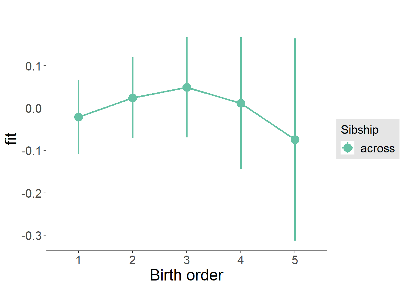
Add Interaction
Model Summary
m4_interaction = update(m3_birthorder_nonlinear, formula = . ~ . - birth_order_nonlinear - sibling_count + count_birth_order)
tidy(m4_interaction, conf.int = T, conf.level = 0.995)| effect | group | term | estimate | std.error | statistic | df | p.value | conf.low | conf.high |
|---|---|---|---|---|---|---|---|---|---|
| fixed | NA | (Intercept) | 1.109 | 0.5499 | 2.016 | 3950 | 0.04383 | -0.4348 | 2.652 |
| fixed | NA | poly(age, 3, raw = TRUE)1 | -0.09522 | 0.0641 | -1.486 | 3947 | 0.1375 | -0.2752 | 0.08471 |
| fixed | NA | poly(age, 3, raw = TRUE)2 | 0.00307 | 0.002362 | 1.3 | 3942 | 0.1938 | -0.003561 | 0.009701 |
| fixed | NA | poly(age, 3, raw = TRUE)3 | -0.00003175 | 0.00002768 | -1.147 | 3937 | 0.2514 | -0.0001095 | 0.00004595 |
| fixed | NA | male | -0.2348 | 0.02989 | -7.853 | 3950 | 5.188e-15 | -0.3187 | -0.1508 |
| fixed | NA | count_birth_order2/2 | 0.04884 | 0.06475 | 0.7544 | 3412 | 0.4507 | -0.1329 | 0.2306 |
| fixed | NA | count_birth_order1/3 | -0.1645 | 0.05586 | -2.946 | 3953 | 0.003241 | -0.3213 | -0.007746 |
| fixed | NA | count_birth_order2/3 | -0.02636 | 0.06051 | -0.4356 | 3954 | 0.6632 | -0.1962 | 0.1435 |
| fixed | NA | count_birth_order3/3 | 0.0319 | 0.06835 | 0.4667 | 3953 | 0.6407 | -0.16 | 0.2238 |
| fixed | NA | count_birth_order1/4 | 0.002842 | 0.06645 | 0.04277 | 3952 | 0.9659 | -0.1837 | 0.1894 |
| fixed | NA | count_birth_order2/4 | -0.04257 | 0.06724 | -0.6332 | 3954 | 0.5266 | -0.2313 | 0.1462 |
| fixed | NA | count_birth_order3/4 | -0.1127 | 0.07465 | -1.509 | 3952 | 0.1313 | -0.3222 | 0.09687 |
| fixed | NA | count_birth_order4/4 | 0.03027 | 0.07651 | 0.3956 | 3951 | 0.6924 | -0.1845 | 0.245 |
| fixed | NA | count_birth_order1/5 | 0.01054 | 0.07925 | 0.133 | 3953 | 0.8942 | -0.2119 | 0.233 |
| fixed | NA | count_birth_order2/5 | -0.0534 | 0.0846 | -0.6312 | 3954 | 0.528 | -0.2909 | 0.1841 |
| fixed | NA | count_birth_order3/5 | 0.05969 | 0.08283 | 0.7206 | 3952 | 0.4712 | -0.1728 | 0.2922 |
| fixed | NA | count_birth_order4/5 | -0.1003 | 0.08434 | -1.189 | 3950 | 0.2346 | -0.337 | 0.1365 |
| fixed | NA | count_birth_order5/5 | -0.108 | 0.08585 | -1.258 | 3945 | 0.2083 | -0.349 | 0.1329 |
| ran_pars | mother_pidlink | sd__(Intercept) | 0.155 | NA | NA | NA | NA | NA | NA |
| ran_pars | Residual | sd__Observation | 0.926 | NA | NA | NA | NA | NA | NA |
Coefficient Plot
plot_birthorder(m4_interaction)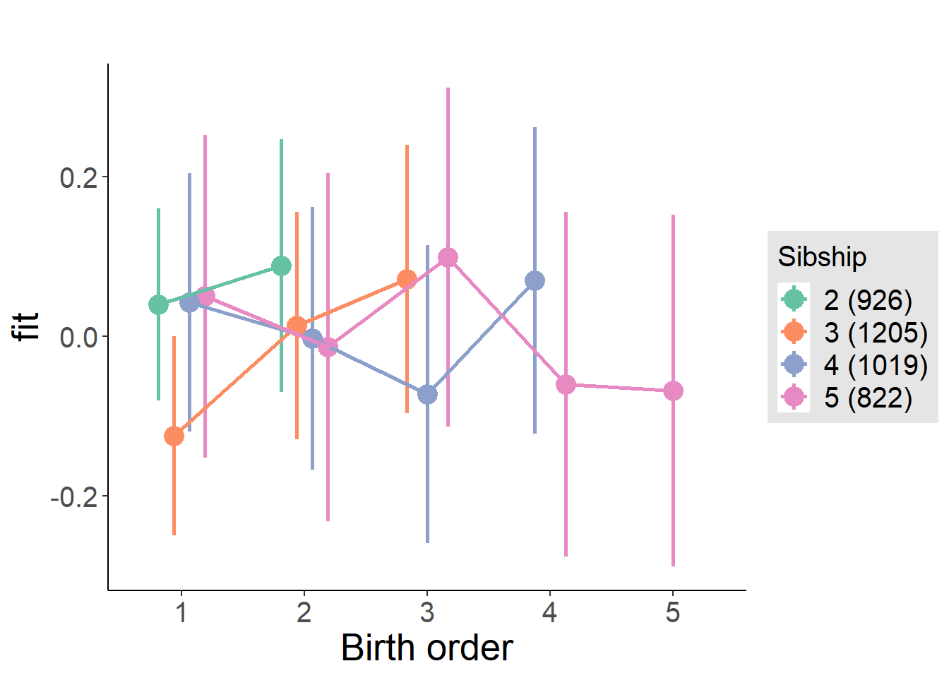
Model Comparison
###### Model 1 - Model 2
anova(m1_covariates_only, m2_birthorder_linear, m3_birthorder_nonlinear, m4_interaction)## refitting model(s) with ML (instead of REML)| Df | AIC | BIC | logLik | deviance | Chisq | Chi Df | Pr(>Chisq) |
|---|---|---|---|---|---|---|---|
| 10 | 10789 | 10852 | -5384 | 10769 | NA | NA | NA |
| 11 | 10790 | 10859 | -5384 | 10768 | 0.4226 | 1 | 0.5156 |
| 14 | 10793 | 10881 | -5382 | 10765 | 3.605 | 3 | 0.3074 |
| 20 | 10792 | 10917 | -5376 | 10752 | 12.98 | 6 | 0.04339 |
Parental full sibling order
outcome_parental_m1 <- update(m2_birthorder_linear, data = birthorder %>%
mutate(sibling_count = sibling_count_genes_factor,
birth_order_nonlinear = birthorder_genes_factor,
birth_order = birthorder_genes,
count_birth_order = count_birthorder_genes
) %>%
filter(sibling_count != "1"))
compare_models_markdown(outcome_parental_m1)Basic Model
Model Summary
m1_covariates_only <- update(m2_birthorder_linear, formula = . ~ . - birth_order)
tidy(m1_covariates_only, conf.int = T, conf.level = 0.995)| effect | group | term | estimate | std.error | statistic | df | p.value | conf.low | conf.high |
|---|---|---|---|---|---|---|---|---|---|
| fixed | NA | (Intercept) | 1.151 | 0.5349 | 2.151 | 4247 | 0.03151 | -0.3508 | 2.652 |
| fixed | NA | poly(age, 3, raw = TRUE)1 | -0.0983 | 0.06246 | -1.574 | 4242 | 0.1156 | -0.2736 | 0.07702 |
| fixed | NA | poly(age, 3, raw = TRUE)2 | 0.003034 | 0.002304 | 1.317 | 4237 | 0.188 | -0.003434 | 0.009502 |
| fixed | NA | poly(age, 3, raw = TRUE)3 | -0.00002951 | 0.00002705 | -1.091 | 4232 | 0.2753 | -0.0001054 | 0.00004641 |
| fixed | NA | male | -0.2306 | 0.02865 | -8.05 | 4246 | 1.063e-15 | -0.311 | -0.1502 |
| fixed | NA | sibling_count3 | -0.04499 | 0.03751 | -1.199 | 3155 | 0.2305 | -0.1503 | 0.06032 |
| fixed | NA | sibling_count4 | -0.01041 | 0.04058 | -0.2566 | 2687 | 0.7975 | -0.1243 | 0.1035 |
| fixed | NA | sibling_count5 | 0.005122 | 0.04744 | 0.108 | 2179 | 0.914 | -0.128 | 0.1383 |
| ran_pars | mother_pidlink | sd__(Intercept) | 0.1631 | NA | NA | NA | NA | NA | NA |
| ran_pars | Residual | sd__Observation | 0.9178 | NA | NA | NA | NA | NA | NA |
Coefficient Plot
plot(allEffects(m1_covariates_only, confidence.level = 0.995))
Add Birth Order Linear
Model Summary
tidy(m2_birthorder_linear, conf.int = T, conf.level = 0.995)| effect | group | term | estimate | std.error | statistic | df | p.value | conf.low | conf.high |
|---|---|---|---|---|---|---|---|---|---|
| fixed | NA | (Intercept) | 1.137 | 0.5355 | 2.123 | 4246 | 0.03379 | -0.3661 | 2.64 |
| fixed | NA | birth_order | 0.008813 | 0.01533 | 0.575 | 4019 | 0.5653 | -0.03421 | 0.05184 |
| fixed | NA | poly(age, 3, raw = TRUE)1 | -0.09791 | 0.06247 | -1.567 | 4242 | 0.1171 | -0.2733 | 0.07744 |
| fixed | NA | poly(age, 3, raw = TRUE)2 | 0.00301 | 0.002305 | 1.306 | 4236 | 0.1917 | -0.00346 | 0.009479 |
| fixed | NA | poly(age, 3, raw = TRUE)3 | -0.00002906 | 0.00002706 | -1.074 | 4231 | 0.283 | -0.000105 | 0.0000469 |
| fixed | NA | male | -0.2309 | 0.02865 | -8.058 | 4244 | 9.979e-16 | -0.3113 | -0.1505 |
| fixed | NA | sibling_count3 | -0.049 | 0.03817 | -1.284 | 3210 | 0.1993 | -0.1561 | 0.05814 |
| fixed | NA | sibling_count4 | -0.0196 | 0.04364 | -0.4492 | 2937 | 0.6533 | -0.1421 | 0.1029 |
| fixed | NA | sibling_count5 | -0.009626 | 0.05395 | -0.1784 | 2660 | 0.8584 | -0.1611 | 0.1418 |
| ran_pars | mother_pidlink | sd__(Intercept) | 0.1647 | NA | NA | NA | NA | NA | NA |
| ran_pars | Residual | sd__Observation | 0.9176 | NA | NA | NA | NA | NA | NA |
Coefficient Plot
plot_birthorder2(m2_birthorder_linear, separate = FALSE)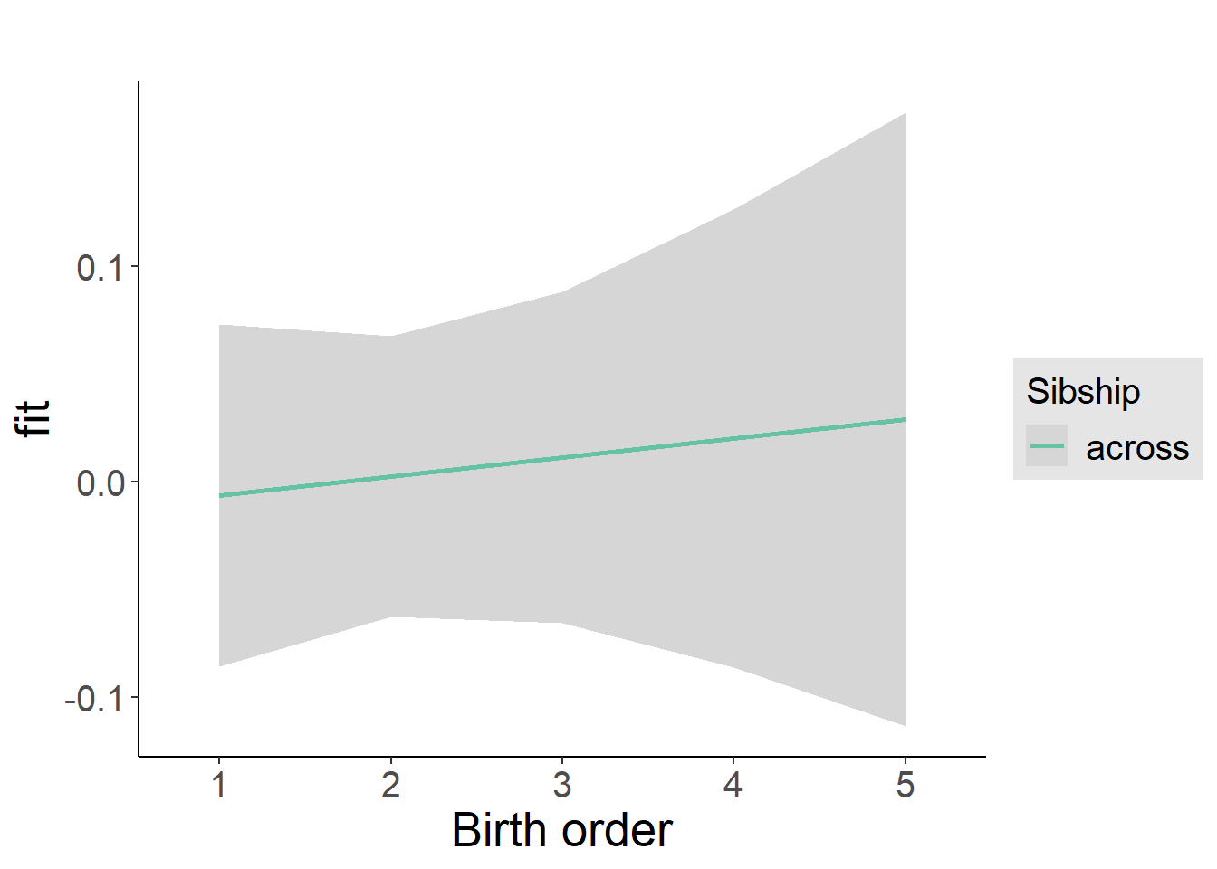
Add Birth Order Factor
Model Summary
m3_birthorder_nonlinear = update(m1_covariates_only, formula = . ~ . + birth_order_nonlinear)
tidy(m3_birthorder_nonlinear, conf.int = T, conf.level = 0.995)| effect | group | term | estimate | std.error | statistic | df | p.value | conf.low | conf.high |
|---|---|---|---|---|---|---|---|---|---|
| fixed | NA | (Intercept) | 1.109 | 0.5358 | 2.069 | 4240 | 0.0386 | -0.3953 | 2.612 |
| fixed | NA | poly(age, 3, raw = TRUE)1 | -0.0946 | 0.06251 | -1.513 | 4236 | 0.1303 | -0.2701 | 0.08089 |
| fixed | NA | poly(age, 3, raw = TRUE)2 | 0.002889 | 0.002307 | 1.252 | 4231 | 0.2105 | -0.003586 | 0.009363 |
| fixed | NA | poly(age, 3, raw = TRUE)3 | -0.00002773 | 0.00002708 | -1.024 | 4226 | 0.3058 | -0.0001037 | 0.00004828 |
| fixed | NA | male | -0.2299 | 0.02866 | -8.02 | 4242 | 1.353e-15 | -0.3104 | -0.1494 |
| fixed | NA | sibling_count3 | -0.05602 | 0.03886 | -1.442 | 3337 | 0.1495 | -0.1651 | 0.05306 |
| fixed | NA | sibling_count4 | -0.0239 | 0.04436 | -0.5389 | 3041 | 0.59 | -0.1484 | 0.1006 |
| fixed | NA | sibling_count5 | 0.005893 | 0.05508 | 0.107 | 2742 | 0.9148 | -0.1487 | 0.1605 |
| fixed | NA | birth_order_nonlinear2 | 0.03567 | 0.03429 | 1.04 | 3533 | 0.2983 | -0.06058 | 0.1319 |
| fixed | NA | birth_order_nonlinear3 | 0.05136 | 0.04374 | 1.174 | 3748 | 0.2404 | -0.07142 | 0.1741 |
| fixed | NA | birth_order_nonlinear4 | 0.02078 | 0.05996 | 0.3465 | 3939 | 0.729 | -0.1475 | 0.1891 |
| fixed | NA | birth_order_nonlinear5 | -0.05124 | 0.09844 | -0.5205 | 3930 | 0.6027 | -0.3276 | 0.2251 |
| ran_pars | mother_pidlink | sd__(Intercept) | 0.1628 | NA | NA | NA | NA | NA | NA |
| ran_pars | Residual | sd__Observation | 0.918 | NA | NA | NA | NA | NA | NA |
Coefficient Plot
plot_birthorder(m3_birthorder_nonlinear, separate = FALSE)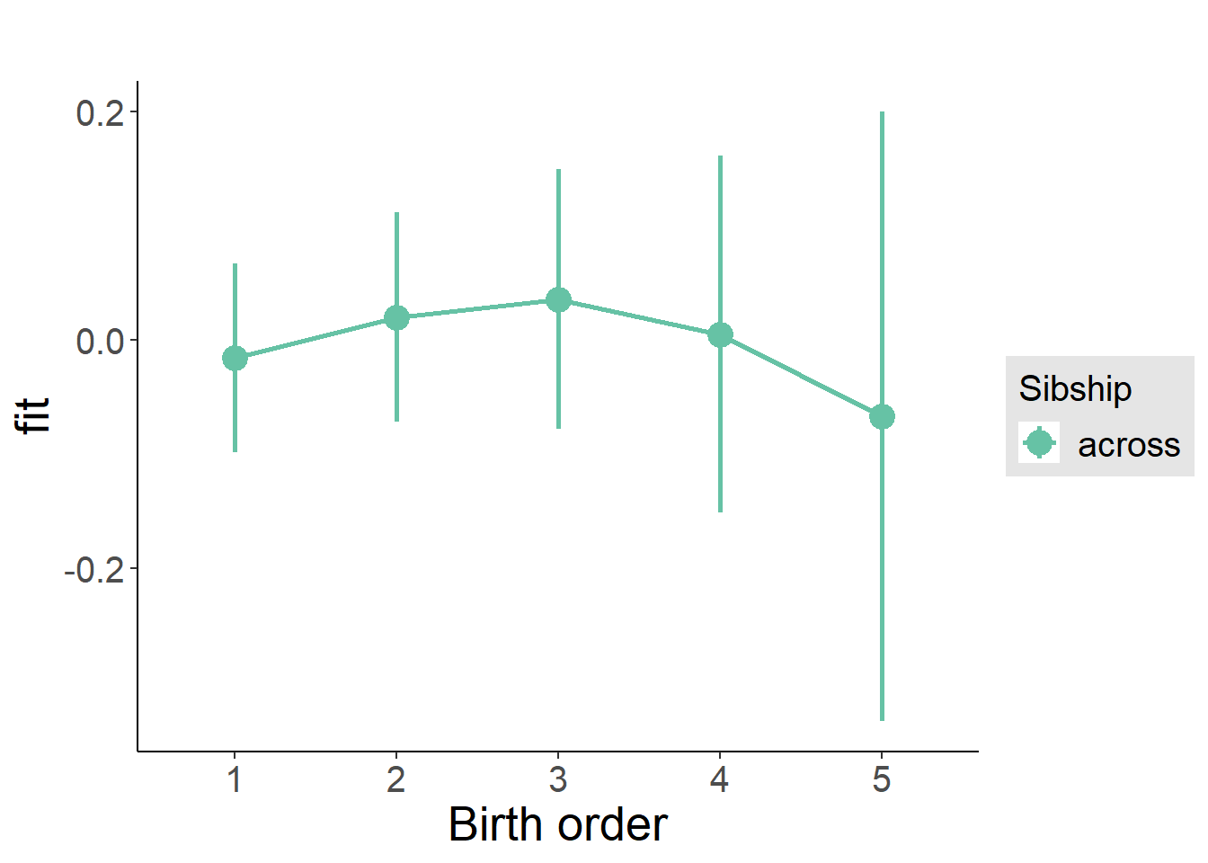
Add Interaction
Model Summary
m4_interaction = update(m3_birthorder_nonlinear, formula = . ~ . - birth_order_nonlinear - sibling_count + count_birth_order)
tidy(m4_interaction, conf.int = T, conf.level = 0.995)| effect | group | term | estimate | std.error | statistic | df | p.value | conf.low | conf.high |
|---|---|---|---|---|---|---|---|---|---|
| fixed | NA | (Intercept) | 1.082 | 0.5356 | 2.021 | 4235 | 0.04339 | -0.4212 | 2.585 |
| fixed | NA | poly(age, 3, raw = TRUE)1 | -0.09134 | 0.06249 | -1.462 | 4231 | 0.1439 | -0.2667 | 0.08406 |
| fixed | NA | poly(age, 3, raw = TRUE)2 | 0.00281 | 0.002305 | 1.219 | 4226 | 0.223 | -0.003661 | 0.009281 |
| fixed | NA | poly(age, 3, raw = TRUE)3 | -0.00002729 | 0.00002707 | -1.008 | 4221 | 0.3134 | -0.0001033 | 0.00004869 |
| fixed | NA | male | -0.2288 | 0.02865 | -7.987 | 4235 | 1.773e-15 | -0.3093 | -0.1484 |
| fixed | NA | count_birth_order2/2 | 0.006322 | 0.05726 | 0.1104 | 3613 | 0.9121 | -0.1544 | 0.1671 |
| fixed | NA | count_birth_order1/3 | -0.1299 | 0.05063 | -2.565 | 4237 | 0.01036 | -0.272 | 0.01226 |
| fixed | NA | count_birth_order2/3 | 0.02053 | 0.05597 | 0.3668 | 4239 | 0.7138 | -0.1366 | 0.1777 |
| fixed | NA | count_birth_order3/3 | 0.03731 | 0.06161 | 0.6056 | 4237 | 0.5448 | -0.1356 | 0.2102 |
| fixed | NA | count_birth_order1/4 | 0.02521 | 0.06337 | 0.3978 | 4238 | 0.6908 | -0.1527 | 0.2031 |
| fixed | NA | count_birth_order2/4 | -0.009462 | 0.06525 | -0.145 | 4239 | 0.8847 | -0.1926 | 0.1737 |
| fixed | NA | count_birth_order3/4 | -0.06088 | 0.06805 | -0.8947 | 4236 | 0.371 | -0.2519 | 0.1301 |
| fixed | NA | count_birth_order4/4 | 0.005436 | 0.0719 | 0.0756 | 4234 | 0.9397 | -0.1964 | 0.2073 |
| fixed | NA | count_birth_order1/5 | 0.09169 | 0.08652 | 1.06 | 4239 | 0.2893 | -0.1512 | 0.3346 |
| fixed | NA | count_birth_order2/5 | -0.06964 | 0.09387 | -0.7419 | 4238 | 0.4582 | -0.3332 | 0.1939 |
| fixed | NA | count_birth_order3/5 | 0.06613 | 0.08935 | 0.7402 | 4236 | 0.4592 | -0.1847 | 0.3169 |
| fixed | NA | count_birth_order4/5 | -0.01503 | 0.08618 | -0.1745 | 4235 | 0.8615 | -0.2569 | 0.2269 |
| fixed | NA | count_birth_order5/5 | -0.05657 | 0.09245 | -0.6118 | 4232 | 0.5407 | -0.3161 | 0.203 |
| ran_pars | mother_pidlink | sd__(Intercept) | 0.1623 | NA | NA | NA | NA | NA | NA |
| ran_pars | Residual | sd__Observation | 0.9175 | NA | NA | NA | NA | NA | NA |
Coefficient Plot
plot_birthorder(m4_interaction)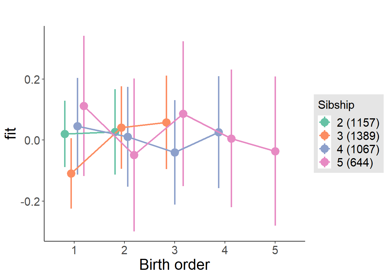
Model Comparison
###### Model 1 - Model 2
anova(m1_covariates_only, m2_birthorder_linear, m3_birthorder_nonlinear, m4_interaction)## refitting model(s) with ML (instead of REML)| Df | AIC | BIC | logLik | deviance | Chisq | Chi Df | Pr(>Chisq) |
|---|---|---|---|---|---|---|---|
| 10 | 11494 | 11557 | -5737 | 11474 | NA | NA | NA |
| 11 | 11495 | 11565 | -5737 | 11473 | 0.3282 | 1 | 0.5667 |
| 14 | 11499 | 11588 | -5736 | 11471 | 2.193 | 3 | 0.5333 |
| 20 | 11499 | 11626 | -5730 | 11459 | 11.88 | 6 | 0.0647 |
Compare birth order specifications
library(coefplot)
multiplot(outcome_naive_m1, outcome_preg_m1, outcome_uterus_m1, outcome_parental_m1, dodgeHeight = 0.6,
intercept = FALSE)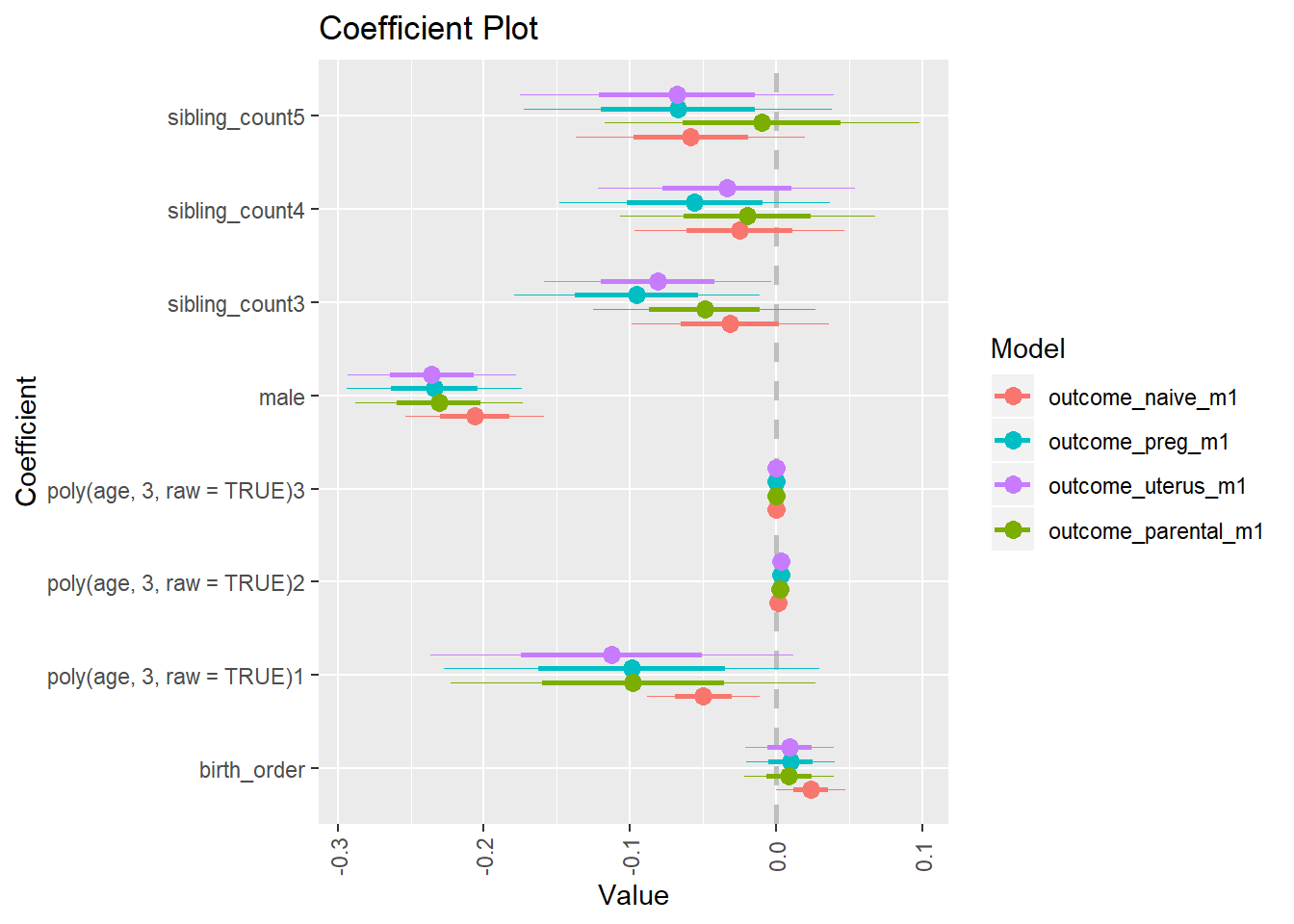
Educational Attainment
Years of Education - z-standardized
birthorder <- birthorder %>% mutate(outcome = years_of_education_z)
model = lmer(outcome ~ birth_order + poly(age, 3, raw = TRUE) + male + sibling_count + (1 | mother_pidlink),
data = birthorder)
compare_birthorder_specs(model)Naive birth order
outcome_naive_m1 <- update(m2_birthorder_linear, data = birthorder %>%
mutate(sibling_count = sibling_count_naive_factor,
birth_order_nonlinear = birthorder_naive_factor,
birth_order = birthorder_naive,
count_birth_order = count_birthorder_naive) %>%
filter(sibling_count != "1"))
compare_models_markdown(outcome_naive_m1)Basic Model
Model Summary
m1_covariates_only <- update(m2_birthorder_linear, formula = . ~ . - birth_order)
tidy(m1_covariates_only, conf.int = T, conf.level = 0.995)| effect | group | term | estimate | std.error | statistic | df | p.value | conf.low | conf.high |
|---|---|---|---|---|---|---|---|---|---|
| fixed | NA | (Intercept) | -3.464 | 0.1642 | -21.09 | 7234 | 7.129e-96 | -3.925 | -3.003 |
| fixed | NA | poly(age, 3, raw = TRUE)1 | 0.3301 | 0.01567 | 21.07 | 7194 | 1.22e-95 | 0.2861 | 0.374 |
| fixed | NA | poly(age, 3, raw = TRUE)2 | -0.008606 | 0.000455 | -18.91 | 7217 | 6.655e-78 | -0.009883 | -0.007329 |
| fixed | NA | poly(age, 3, raw = TRUE)3 | 0.00006344 | 0.000004092 | 15.5 | 7232 | 2.345e-53 | 0.00005196 | 0.00007493 |
| fixed | NA | male | -0.016 | 0.01828 | -0.8752 | 6039 | 0.3815 | -0.0673 | 0.0353 |
| fixed | NA | sibling_count3 | 0.06858 | 0.03289 | 2.085 | 5172 | 0.03711 | -0.02374 | 0.1609 |
| fixed | NA | sibling_count4 | 0.02168 | 0.03451 | 0.6282 | 4980 | 0.5299 | -0.07519 | 0.1185 |
| fixed | NA | sibling_count5 | 0.005908 | 0.03661 | 0.1613 | 4801 | 0.8718 | -0.09687 | 0.1087 |
| ran_pars | mother_pidlink | sd__(Intercept) | 0.6653 | NA | NA | NA | NA | NA | NA |
| ran_pars | Residual | sd__Observation | 0.6199 | NA | NA | NA | NA | NA | NA |
Coefficient Plot
plot(allEffects(m1_covariates_only, confidence.level = 0.995))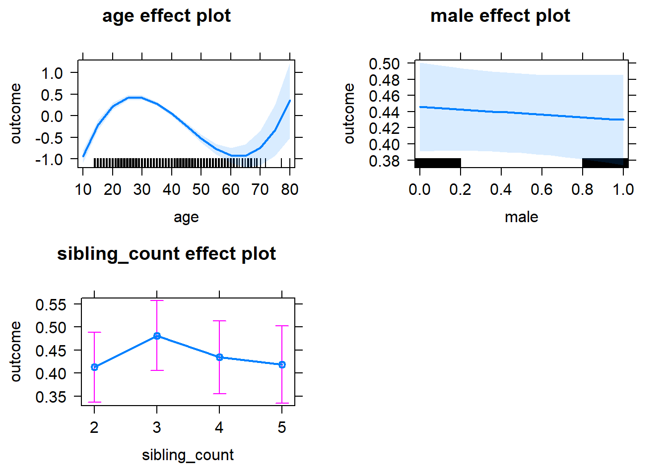
Add Birth Order Linear
Model Summary
tidy(m2_birthorder_linear, conf.int = T, conf.level = 0.995)| effect | group | term | estimate | std.error | statistic | df | p.value | conf.low | conf.high |
|---|---|---|---|---|---|---|---|---|---|
| fixed | NA | (Intercept) | -3.446 | 0.1646 | -20.94 | 7270 | 1.428e-94 | -3.908 | -2.984 |
| fixed | NA | birth_order | -0.0135 | 0.0087 | -1.551 | 5659 | 0.1209 | -0.03792 | 0.01092 |
| fixed | NA | poly(age, 3, raw = TRUE)1 | 0.3308 | 0.01567 | 21.11 | 7179 | 5.297e-96 | 0.2868 | 0.3748 |
| fixed | NA | poly(age, 3, raw = TRUE)2 | -0.008635 | 0.0004553 | -18.96 | 7209 | 2.631e-78 | -0.009914 | -0.007357 |
| fixed | NA | poly(age, 3, raw = TRUE)3 | 0.00006364 | 0.000004093 | 15.55 | 7227 | 1.215e-53 | 0.00005215 | 0.00007513 |
| fixed | NA | male | -0.01579 | 0.01827 | -0.8639 | 6034 | 0.3877 | -0.06707 | 0.0355 |
| fixed | NA | sibling_count3 | 0.07232 | 0.03298 | 2.193 | 5237 | 0.02837 | -0.02026 | 0.1649 |
| fixed | NA | sibling_count4 | 0.03143 | 0.03508 | 0.8958 | 5268 | 0.3704 | -0.06705 | 0.1299 |
| fixed | NA | sibling_count5 | 0.02279 | 0.03821 | 0.5966 | 5406 | 0.5508 | -0.08446 | 0.13 |
| ran_pars | mother_pidlink | sd__(Intercept) | 0.6657 | NA | NA | NA | NA | NA | NA |
| ran_pars | Residual | sd__Observation | 0.6196 | NA | NA | NA | NA | NA | NA |
Coefficient Plot
plot_birthorder2(m2_birthorder_linear, separate = FALSE)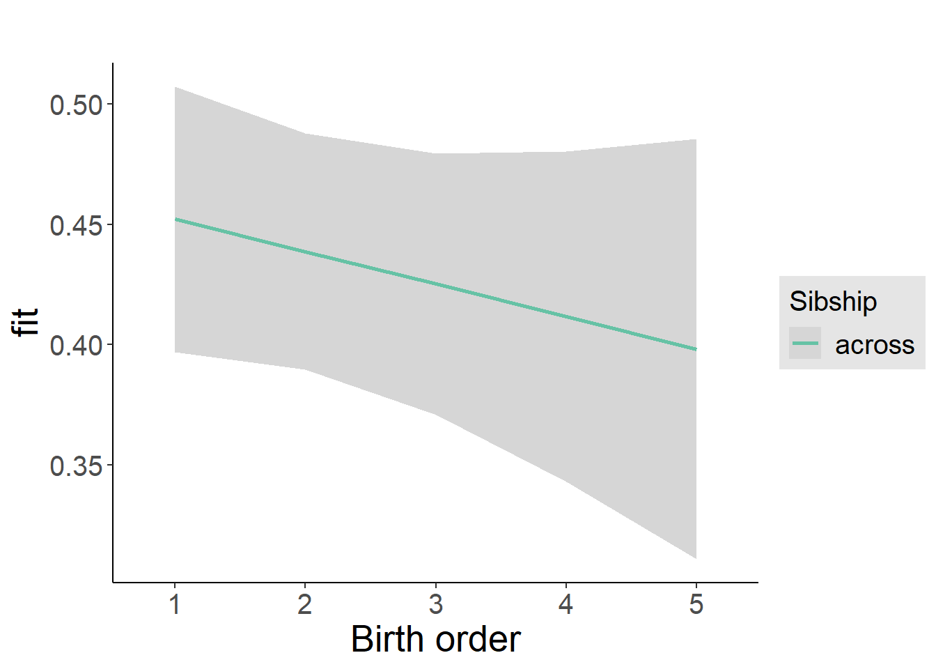
Add Birth Order Factor
Model Summary
m3_birthorder_nonlinear = update(m1_covariates_only, formula = . ~ . + birth_order_nonlinear)
tidy(m3_birthorder_nonlinear, conf.int = T, conf.level = 0.995)| effect | group | term | estimate | std.error | statistic | df | p.value | conf.low | conf.high |
|---|---|---|---|---|---|---|---|---|---|
| fixed | NA | (Intercept) | -3.431 | 0.1645 | -20.86 | 7246 | 7.049e-94 | -3.893 | -2.969 |
| fixed | NA | poly(age, 3, raw = TRUE)1 | 0.3287 | 0.01567 | 20.97 | 7185 | 7.587e-95 | 0.2847 | 0.3727 |
| fixed | NA | poly(age, 3, raw = TRUE)2 | -0.008538 | 0.0004558 | -18.73 | 7223 | 1.719e-76 | -0.009818 | -0.007259 |
| fixed | NA | poly(age, 3, raw = TRUE)3 | 0.00006246 | 0.000004103 | 15.22 | 7251 | 1.547e-51 | 0.00005094 | 0.00007398 |
| fixed | NA | male | -0.01519 | 0.01823 | -0.8334 | 6017 | 0.4047 | -0.06637 | 0.03599 |
| fixed | NA | sibling_count3 | 0.0825 | 0.03321 | 2.484 | 5347 | 0.01302 | -0.01072 | 0.1757 |
| fixed | NA | sibling_count4 | 0.04427 | 0.03533 | 1.253 | 5385 | 0.2103 | -0.05491 | 0.1435 |
| fixed | NA | sibling_count5 | 0.0107 | 0.03834 | 0.2792 | 5479 | 0.7801 | -0.09691 | 0.1183 |
| fixed | NA | birth_order_nonlinear2 | -0.06449 | 0.02051 | -3.144 | 5341 | 0.001674 | -0.1221 | -0.006916 |
| fixed | NA | birth_order_nonlinear3 | -0.08792 | 0.026 | -3.382 | 5125 | 0.0007246 | -0.1609 | -0.01495 |
| fixed | NA | birth_order_nonlinear4 | -0.07154 | 0.03388 | -2.112 | 5069 | 0.03477 | -0.1667 | 0.02356 |
| fixed | NA | birth_order_nonlinear5 | 0.08977 | 0.04907 | 1.829 | 4784 | 0.0674 | -0.04797 | 0.2275 |
| ran_pars | mother_pidlink | sd__(Intercept) | 0.6666 | NA | NA | NA | NA | NA | NA |
| ran_pars | Residual | sd__Observation | 0.6176 | NA | NA | NA | NA | NA | NA |
Coefficient Plot
plot_birthorder(m3_birthorder_nonlinear, separate = FALSE)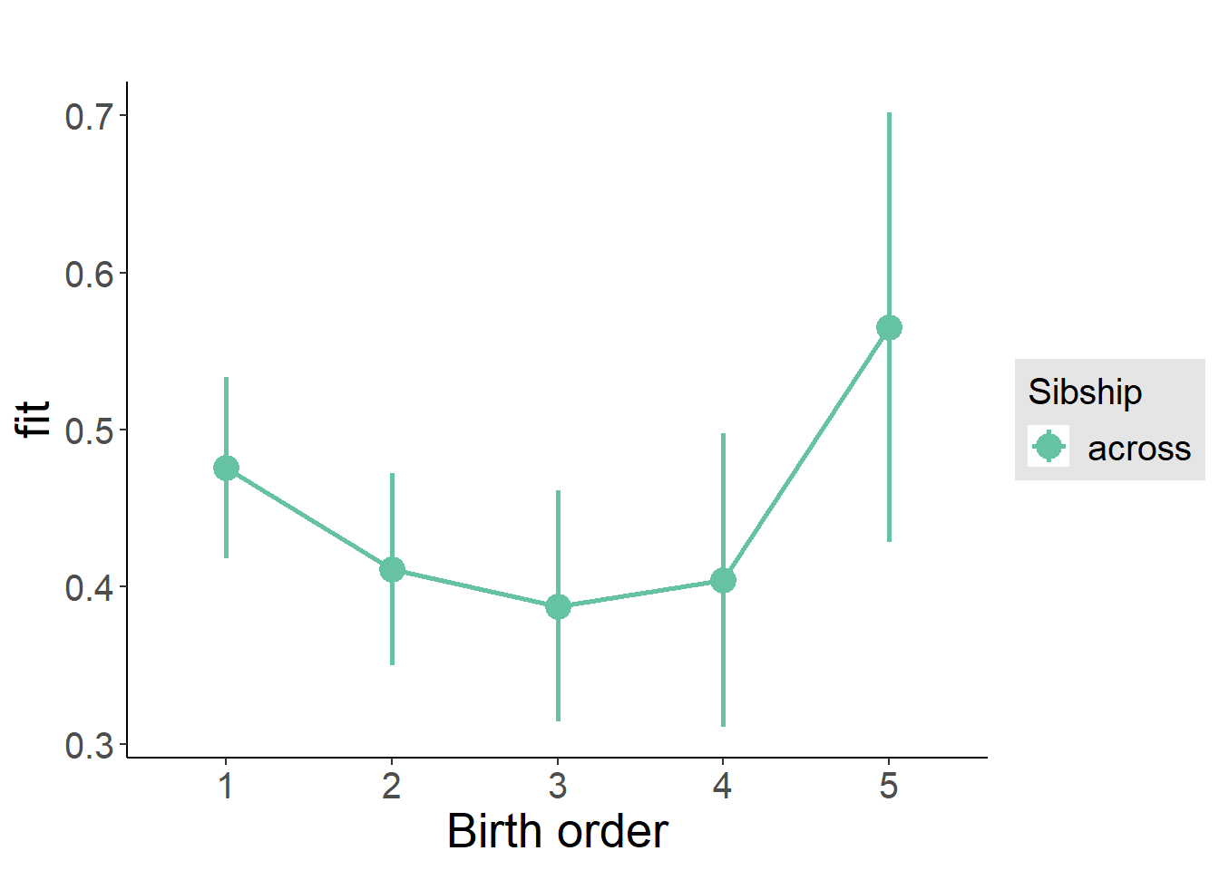
Add Interaction
Model Summary
m4_interaction = update(m3_birthorder_nonlinear, formula = . ~ . - birth_order_nonlinear - sibling_count + count_birth_order)
tidy(m4_interaction, conf.int = T, conf.level = 0.995)| effect | group | term | estimate | std.error | statistic | df | p.value | conf.low | conf.high |
|---|---|---|---|---|---|---|---|---|---|
| fixed | NA | (Intercept) | -3.424 | 0.1648 | -20.78 | 7240 | 3.585e-93 | -3.886 | -2.961 |
| fixed | NA | poly(age, 3, raw = TRUE)1 | 0.3287 | 0.01568 | 20.96 | 7180 | 9.111e-95 | 0.2847 | 0.3727 |
| fixed | NA | poly(age, 3, raw = TRUE)2 | -0.008534 | 0.000456 | -18.71 | 7219 | 2.379e-76 | -0.009814 | -0.007254 |
| fixed | NA | poly(age, 3, raw = TRUE)3 | 0.00006239 | 0.000004106 | 15.19 | 7250 | 2.362e-51 | 0.00005086 | 0.00007392 |
| fixed | NA | male | -0.01526 | 0.01824 | -0.8368 | 6006 | 0.4027 | -0.06645 | 0.03593 |
| fixed | NA | count_birth_order2/2 | -0.08721 | 0.03507 | -2.486 | 5491 | 0.01293 | -0.1857 | 0.01124 |
| fixed | NA | count_birth_order1/3 | 0.07269 | 0.03884 | 1.872 | 6994 | 0.06131 | -0.03633 | 0.1817 |
| fixed | NA | count_birth_order2/3 | 0.01095 | 0.04268 | 0.2566 | 7314 | 0.7975 | -0.1089 | 0.1308 |
| fixed | NA | count_birth_order3/3 | -0.01067 | 0.04684 | -0.2279 | 7433 | 0.8197 | -0.1422 | 0.1208 |
| fixed | NA | count_birth_order1/4 | 0.02226 | 0.04328 | 0.5143 | 7252 | 0.607 | -0.09923 | 0.1438 |
| fixed | NA | count_birth_order2/4 | -0.03591 | 0.04581 | -0.7839 | 7387 | 0.4331 | -0.1645 | 0.09267 |
| fixed | NA | count_birth_order3/4 | -0.02143 | 0.04878 | -0.4394 | 7436 | 0.6604 | -0.1584 | 0.1155 |
| fixed | NA | count_birth_order4/4 | -0.03057 | 0.05094 | -0.6001 | 7429 | 0.5485 | -0.1736 | 0.1124 |
| fixed | NA | count_birth_order1/5 | 0.004056 | 0.04884 | 0.08305 | 7408 | 0.9338 | -0.133 | 0.1411 |
| fixed | NA | count_birth_order2/5 | -0.02462 | 0.05108 | -0.4819 | 7437 | 0.6299 | -0.168 | 0.1188 |
| fixed | NA | count_birth_order3/5 | -0.1238 | 0.05165 | -2.398 | 7433 | 0.01653 | -0.2688 | 0.02115 |
| fixed | NA | count_birth_order4/5 | -0.07325 | 0.05469 | -1.339 | 7374 | 0.1805 | -0.2268 | 0.08026 |
| fixed | NA | count_birth_order5/5 | 0.09118 | 0.05573 | 1.636 | 7370 | 0.1018 | -0.06524 | 0.2476 |
| ran_pars | mother_pidlink | sd__(Intercept) | 0.6669 | NA | NA | NA | NA | NA | NA |
| ran_pars | Residual | sd__Observation | 0.6176 | NA | NA | NA | NA | NA | NA |
Coefficient Plot
plot_birthorder(m4_interaction)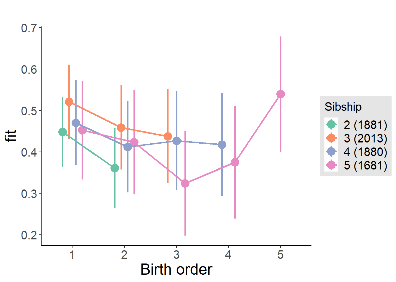
Model Comparison
###### Model 1 - Model 2
anova(m1_covariates_only, m2_birthorder_linear, m3_birthorder_nonlinear, m4_interaction)## refitting model(s) with ML (instead of REML)| Df | AIC | BIC | logLik | deviance | Chisq | Chi Df | Pr(>Chisq) |
|---|---|---|---|---|---|---|---|
| 10 | 18711 | 18780 | -9345 | 18691 | NA | NA | NA |
| 11 | 18710 | 18787 | -9344 | 18688 | 2.406 | 1 | 0.1209 |
| 14 | 18693 | 18790 | -9332 | 18665 | 23.78 | 3 | 0.00002772 |
| 20 | 18701 | 18840 | -9331 | 18661 | 3.483 | 6 | 0.7462 |
Maternal birth order
outcome_uterus_m1 <- update(m2_birthorder_linear, data = birthorder %>%
mutate(sibling_count = sibling_count_uterus_alive_factor,
birth_order_nonlinear = birthorder_uterus_alive_factor,
birth_order = birthorder_uterus_alive,
count_birth_order = count_birthorder_uterus_alive) %>%
filter(sibling_count != "1"))
compare_models_markdown(outcome_uterus_m1)Basic Model
Model Summary
m1_covariates_only <- update(m2_birthorder_linear, formula = . ~ . - birth_order)
tidy(m1_covariates_only, conf.int = T, conf.level = 0.995)| effect | group | term | estimate | std.error | statistic | df | p.value | conf.low | conf.high |
|---|---|---|---|---|---|---|---|---|---|
| fixed | NA | (Intercept) | -7.236 | 0.3724 | -19.43 | 4376 | 9.361e-81 | -8.282 | -6.191 |
| fixed | NA | poly(age, 3, raw = TRUE)1 | 0.7719 | 0.04354 | 17.73 | 4384 | 5.778e-68 | 0.6497 | 0.8942 |
| fixed | NA | poly(age, 3, raw = TRUE)2 | -0.02413 | 0.001609 | -15 | 4403 | 1.225e-49 | -0.02865 | -0.01961 |
| fixed | NA | poly(age, 3, raw = TRUE)3 | 0.0002427 | 0.0000189 | 12.84 | 4428 | 4.355e-37 | 0.0001897 | 0.0002958 |
| fixed | NA | male | -0.08201 | 0.01961 | -4.183 | 4011 | 0.00002939 | -0.137 | -0.02698 |
| fixed | NA | sibling_count3 | 0.0106 | 0.03091 | 0.343 | 3434 | 0.7316 | -0.07615 | 0.09736 |
| fixed | NA | sibling_count4 | -0.0882 | 0.03392 | -2.6 | 3258 | 0.009366 | -0.1834 | 0.007025 |
| fixed | NA | sibling_count5 | -0.174 | 0.0395 | -4.405 | 3145 | 0.00001091 | -0.2849 | -0.06314 |
| ran_pars | mother_pidlink | sd__(Intercept) | 0.4989 | NA | NA | NA | NA | NA | NA |
| ran_pars | Residual | sd__Observation | 0.5371 | NA | NA | NA | NA | NA | NA |
Coefficient Plot
plot(allEffects(m1_covariates_only, confidence.level = 0.995))
Add Birth Order Linear
Model Summary
tidy(m2_birthorder_linear, conf.int = T, conf.level = 0.995)| effect | group | term | estimate | std.error | statistic | df | p.value | conf.low | conf.high |
|---|---|---|---|---|---|---|---|---|---|
| fixed | NA | (Intercept) | -7.28 | 0.3728 | -19.53 | 4384 | 1.672e-81 | -8.326 | -6.234 |
| fixed | NA | birth_order | 0.02178 | 0.01018 | 2.14 | 4070 | 0.03242 | -0.006789 | 0.05034 |
| fixed | NA | poly(age, 3, raw = TRUE)1 | 0.7732 | 0.04353 | 17.76 | 4383 | 3.246e-68 | 0.651 | 0.8954 |
| fixed | NA | poly(age, 3, raw = TRUE)2 | -0.02418 | 0.001608 | -15.04 | 4401 | 7.234e-50 | -0.0287 | -0.01967 |
| fixed | NA | poly(age, 3, raw = TRUE)3 | 0.0002438 | 0.0000189 | 12.9 | 4426 | 2.125e-37 | 0.0001907 | 0.0002968 |
| fixed | NA | male | -0.08264 | 0.0196 | -4.216 | 4011 | 0.00002539 | -0.1377 | -0.02762 |
| fixed | NA | sibling_count3 | -0.00009053 | 0.0313 | -0.002893 | 3481 | 0.9977 | -0.08794 | 0.08776 |
| fixed | NA | sibling_count4 | -0.1131 | 0.03586 | -3.155 | 3418 | 0.001617 | -0.2138 | -0.01249 |
| fixed | NA | sibling_count5 | -0.2147 | 0.04382 | -4.899 | 3521 | 0.000001006 | -0.3377 | -0.09167 |
| ran_pars | mother_pidlink | sd__(Intercept) | 0.4987 | NA | NA | NA | NA | NA | NA |
| ran_pars | Residual | sd__Observation | 0.5369 | NA | NA | NA | NA | NA | NA |
Coefficient Plot
plot_birthorder2(m2_birthorder_linear, separate = FALSE)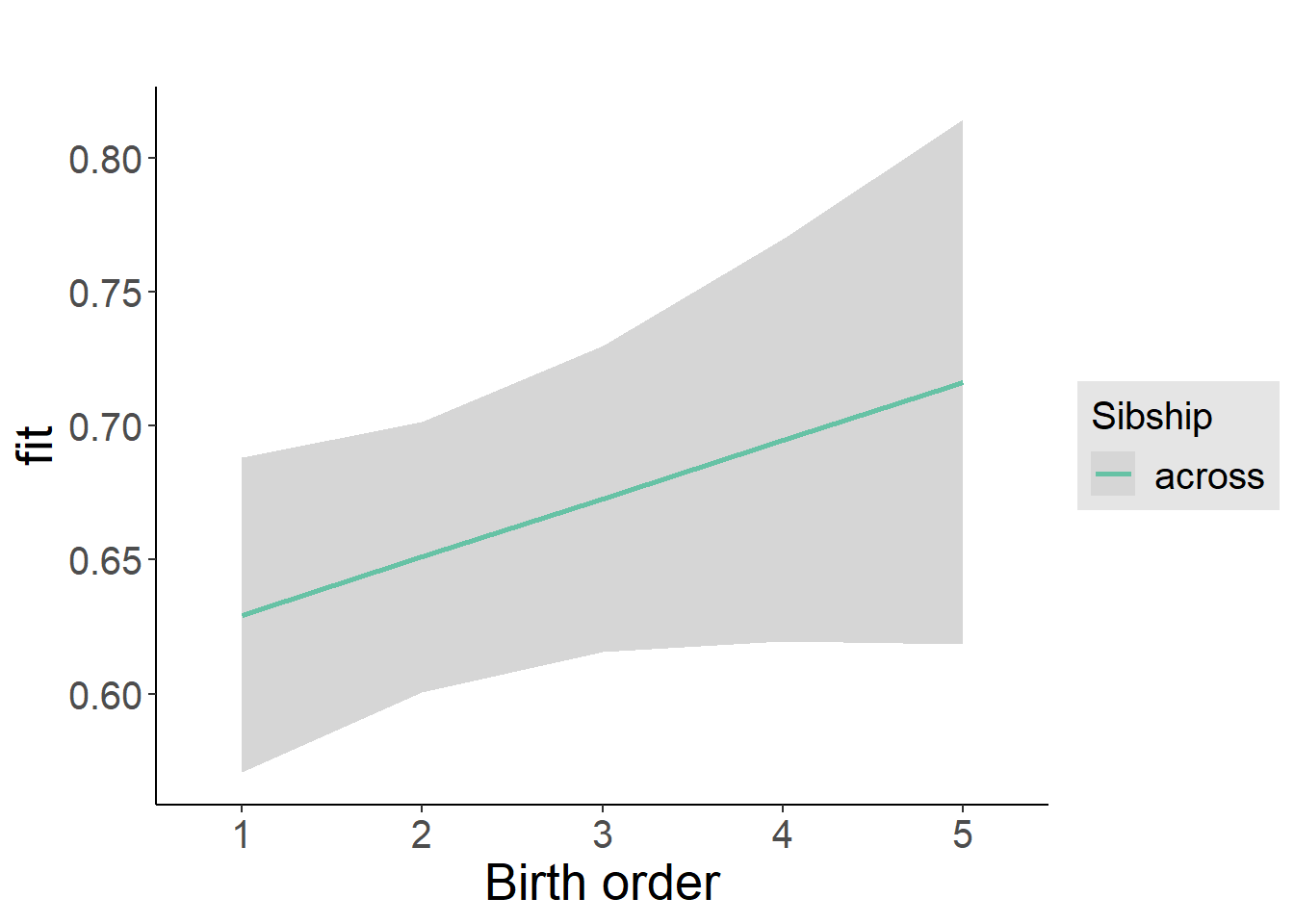
Add Birth Order Factor
Model Summary
m3_birthorder_nonlinear = update(m1_covariates_only, formula = . ~ . + birth_order_nonlinear)
tidy(m3_birthorder_nonlinear, conf.int = T, conf.level = 0.995)| effect | group | term | estimate | std.error | statistic | df | p.value | conf.low | conf.high |
|---|---|---|---|---|---|---|---|---|---|
| fixed | NA | (Intercept) | -7.12 | 0.3736 | -19.06 | 4415 | 7.194e-78 | -8.168 | -6.071 |
| fixed | NA | poly(age, 3, raw = TRUE)1 | 0.7603 | 0.04361 | 17.43 | 4411 | 7.091e-66 | 0.6379 | 0.8827 |
| fixed | NA | poly(age, 3, raw = TRUE)2 | -0.02373 | 0.001611 | -14.74 | 4423 | 5.145e-48 | -0.02825 | -0.01921 |
| fixed | NA | poly(age, 3, raw = TRUE)3 | 0.000239 | 0.00001891 | 12.64 | 4441 | 5.491e-36 | 0.0001859 | 0.0002921 |
| fixed | NA | male | -0.08368 | 0.01957 | -4.276 | 4005 | 0.00001951 | -0.1386 | -0.02874 |
| fixed | NA | sibling_count3 | 0.002044 | 0.03157 | 0.06476 | 3570 | 0.9484 | -0.08657 | 0.09066 |
| fixed | NA | sibling_count4 | -0.1153 | 0.03617 | -3.188 | 3499 | 0.001445 | -0.2168 | -0.01378 |
| fixed | NA | sibling_count5 | -0.2389 | 0.04428 | -5.395 | 3616 | 0.00000007273 | -0.3632 | -0.1146 |
| fixed | NA | birth_order_nonlinear2 | -0.05553 | 0.02208 | -2.515 | 3297 | 0.01197 | -0.1175 | 0.00646 |
| fixed | NA | birth_order_nonlinear3 | 0.03104 | 0.02852 | 1.089 | 3512 | 0.2764 | -0.04901 | 0.1111 |
| fixed | NA | birth_order_nonlinear4 | 0.06363 | 0.0389 | 1.636 | 3698 | 0.1019 | -0.04555 | 0.1728 |
| fixed | NA | birth_order_nonlinear5 | 0.1591 | 0.06017 | 2.644 | 3376 | 0.008232 | -0.009812 | 0.328 |
| ran_pars | mother_pidlink | sd__(Intercept) | 0.4988 | NA | NA | NA | NA | NA | NA |
| ran_pars | Residual | sd__Observation | 0.5357 | NA | NA | NA | NA | NA | NA |
Coefficient Plot
plot_birthorder(m3_birthorder_nonlinear, separate = FALSE)
Add Interaction
Model Summary
m4_interaction = update(m3_birthorder_nonlinear, formula = . ~ . - birth_order_nonlinear - sibling_count + count_birth_order)
tidy(m4_interaction, conf.int = T, conf.level = 0.995)| effect | group | term | estimate | std.error | statistic | df | p.value | conf.low | conf.high |
|---|---|---|---|---|---|---|---|---|---|
| fixed | NA | (Intercept) | -7.118 | 0.3739 | -19.04 | 4414 | 1.015e-77 | -8.168 | -6.068 |
| fixed | NA | poly(age, 3, raw = TRUE)1 | 0.7593 | 0.04363 | 17.4 | 4405 | 1.196e-65 | 0.6368 | 0.8818 |
| fixed | NA | poly(age, 3, raw = TRUE)2 | -0.0237 | 0.001612 | -14.71 | 4417 | 7.629e-48 | -0.02823 | -0.01918 |
| fixed | NA | poly(age, 3, raw = TRUE)3 | 0.0002388 | 0.00001893 | 12.61 | 4435 | 7.403e-36 | 0.0001856 | 0.0002919 |
| fixed | NA | male | -0.08366 | 0.01959 | -4.27 | 4001 | 0.00002 | -0.1387 | -0.02866 |
| fixed | NA | count_birth_order2/2 | -0.03201 | 0.03837 | -0.8343 | 3592 | 0.4041 | -0.1397 | 0.07569 |
| fixed | NA | count_birth_order1/3 | 0.02694 | 0.0376 | 0.7163 | 4546 | 0.4738 | -0.07861 | 0.1325 |
| fixed | NA | count_birth_order2/3 | -0.06356 | 0.04041 | -1.573 | 4655 | 0.1158 | -0.177 | 0.04987 |
| fixed | NA | count_birth_order3/3 | 0.02952 | 0.04463 | 0.6615 | 4661 | 0.5083 | -0.09575 | 0.1548 |
| fixed | NA | count_birth_order1/4 | -0.1223 | 0.04558 | -2.683 | 4645 | 0.007333 | -0.2502 | 0.005674 |
| fixed | NA | count_birth_order2/4 | -0.1747 | 0.04642 | -3.764 | 4665 | 0.0001695 | -0.305 | -0.0444 |
| fixed | NA | count_birth_order3/4 | -0.05508 | 0.0486 | -1.133 | 4623 | 0.2571 | -0.1915 | 0.08133 |
| fixed | NA | count_birth_order4/4 | -0.03078 | 0.05043 | -0.6103 | 4618 | 0.5417 | -0.1723 | 0.1108 |
| fixed | NA | count_birth_order1/5 | -0.2352 | 0.06134 | -3.834 | 4644 | 0.000128 | -0.4073 | -0.06297 |
| fixed | NA | count_birth_order2/5 | -0.241 | 0.06472 | -3.724 | 4489 | 0.0001986 | -0.4227 | -0.05933 |
| fixed | NA | count_birth_order3/5 | -0.2154 | 0.06039 | -3.566 | 4545 | 0.0003655 | -0.3849 | -0.04587 |
| fixed | NA | count_birth_order4/5 | -0.1855 | 0.05906 | -3.142 | 4587 | 0.001691 | -0.3513 | -0.01976 |
| fixed | NA | count_birth_order5/5 | -0.07281 | 0.06096 | -1.194 | 4536 | 0.2324 | -0.2439 | 0.0983 |
| ran_pars | mother_pidlink | sd__(Intercept) | 0.4984 | NA | NA | NA | NA | NA | NA |
| ran_pars | Residual | sd__Observation | 0.5362 | NA | NA | NA | NA | NA | NA |
Coefficient Plot
plot_birthorder(m4_interaction)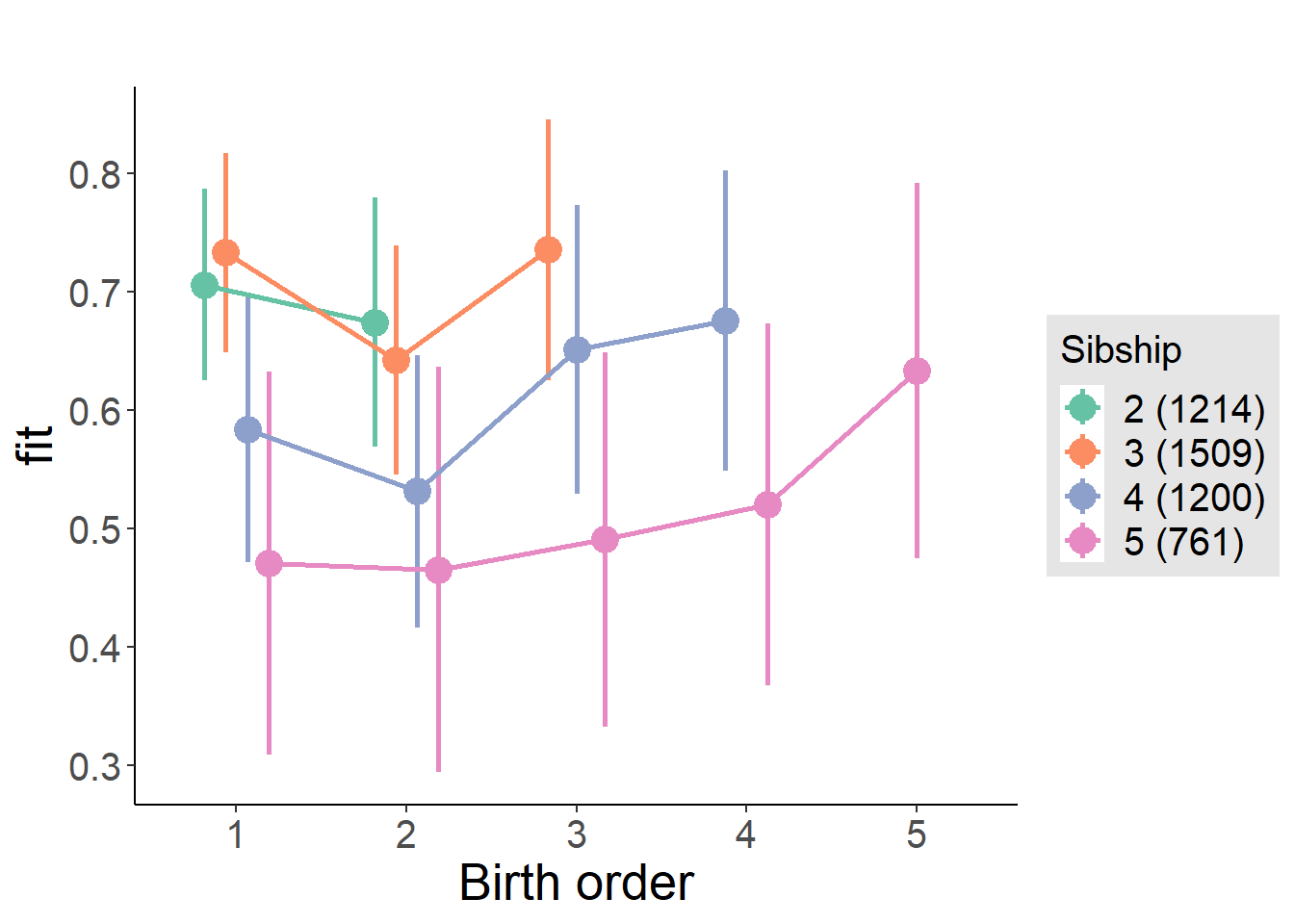
Model Comparison
###### Model 1 - Model 2
anova(m1_covariates_only, m2_birthorder_linear, m3_birthorder_nonlinear, m4_interaction)## refitting model(s) with ML (instead of REML)| Df | AIC | BIC | logLik | deviance | Chisq | Chi Df | Pr(>Chisq) |
|---|---|---|---|---|---|---|---|
| 10 | 9994 | 10058 | -4987 | 9974 | NA | NA | NA |
| 11 | 9991 | 10062 | -4984 | 9969 | 4.586 | 1 | 0.03224 |
| 14 | 9981 | 10071 | -4976 | 9953 | 16.33 | 3 | 0.0009685 |
| 20 | 9989 | 10119 | -4975 | 9949 | 3.115 | 6 | 0.7943 |
Maternal pregnancy order
outcome_preg_m1 <- update(m2_birthorder_linear, data = birthorder %>%
mutate(sibling_count = sibling_count_uterus_preg_factor,
birth_order_nonlinear = birthorder_uterus_preg_factor,
birth_order = birthorder_uterus_preg,
count_birth_order = count_birthorder_uterus_preg
) %>%
filter(sibling_count != "1"))
compare_models_markdown(outcome_preg_m1)Basic Model
Model Summary
m1_covariates_only <- update(m2_birthorder_linear, formula = . ~ . - birth_order)
tidy(m1_covariates_only, conf.int = T, conf.level = 0.995)| effect | group | term | estimate | std.error | statistic | df | p.value | conf.low | conf.high |
|---|---|---|---|---|---|---|---|---|---|
| fixed | NA | (Intercept) | -7.461 | 0.381 | -19.58 | 4064 | 1.135e-81 | -8.531 | -6.392 |
| fixed | NA | poly(age, 3, raw = TRUE)1 | 0.7966 | 0.0446 | 17.86 | 4071 | 9.208e-69 | 0.6714 | 0.9217 |
| fixed | NA | poly(age, 3, raw = TRUE)2 | -0.02504 | 0.001649 | -15.19 | 4092 | 1.018e-50 | -0.02966 | -0.02041 |
| fixed | NA | poly(age, 3, raw = TRUE)3 | 0.0002526 | 0.00001938 | 13.04 | 4120 | 4.317e-38 | 0.0001982 | 0.000307 |
| fixed | NA | male | -0.07778 | 0.02023 | -3.846 | 3720 | 0.0001223 | -0.1346 | -0.02101 |
| fixed | NA | sibling_count3 | 0.0301 | 0.03313 | 0.9086 | 3273 | 0.3636 | -0.06289 | 0.1231 |
| fixed | NA | sibling_count4 | -0.03826 | 0.03541 | -1.08 | 3140 | 0.2801 | -0.1377 | 0.06115 |
| fixed | NA | sibling_count5 | -0.09943 | 0.03854 | -2.58 | 3026 | 0.009935 | -0.2076 | 0.008762 |
| ran_pars | mother_pidlink | sd__(Intercept) | 0.4971 | NA | NA | NA | NA | NA | NA |
| ran_pars | Residual | sd__Observation | 0.5322 | NA | NA | NA | NA | NA | NA |
Coefficient Plot
plot(allEffects(m1_covariates_only, confidence.level = 0.995))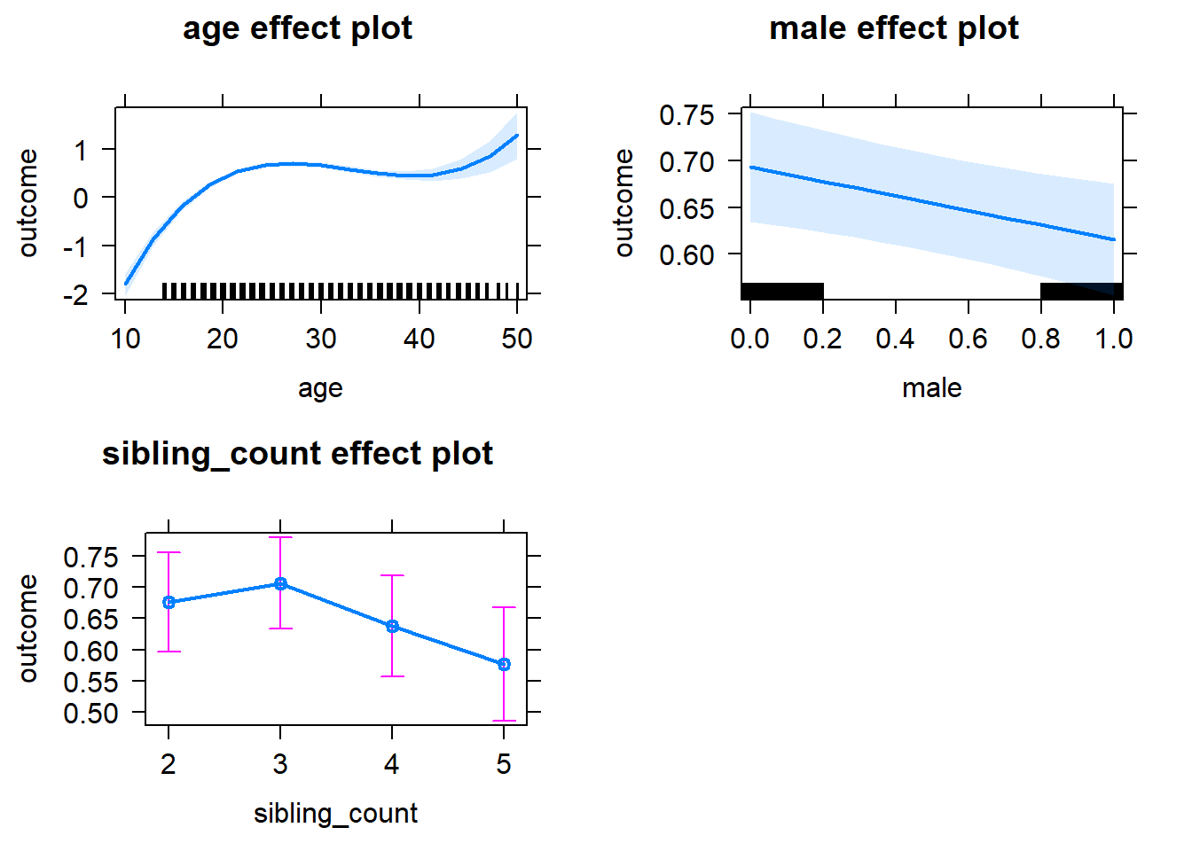
Add Birth Order Linear
Model Summary
tidy(m2_birthorder_linear, conf.int = T, conf.level = 0.995)| effect | group | term | estimate | std.error | statistic | df | p.value | conf.low | conf.high |
|---|---|---|---|---|---|---|---|---|---|
| fixed | NA | (Intercept) | -7.489 | 0.3814 | -19.64 | 4067 | 4.221e-82 | -8.559 | -6.418 |
| fixed | NA | birth_order | 0.01576 | 0.01018 | 1.549 | 3855 | 0.1216 | -0.01281 | 0.04433 |
| fixed | NA | poly(age, 3, raw = TRUE)1 | 0.7969 | 0.04459 | 17.87 | 4070 | 7.591e-69 | 0.6718 | 0.9221 |
| fixed | NA | poly(age, 3, raw = TRUE)2 | -0.02505 | 0.001648 | -15.2 | 4090 | 8.609e-51 | -0.02968 | -0.02043 |
| fixed | NA | poly(age, 3, raw = TRUE)3 | 0.0002531 | 0.00001937 | 13.06 | 4118 | 3.102e-38 | 0.0001987 | 0.0003075 |
| fixed | NA | male | -0.07808 | 0.02022 | -3.861 | 3719 | 0.0001149 | -0.1349 | -0.02131 |
| fixed | NA | sibling_count3 | 0.02236 | 0.0335 | 0.6676 | 3306 | 0.5045 | -0.07167 | 0.1164 |
| fixed | NA | sibling_count4 | -0.05558 | 0.03713 | -1.497 | 3257 | 0.1346 | -0.1598 | 0.04866 |
| fixed | NA | sibling_count5 | -0.1268 | 0.0424 | -2.991 | 3300 | 0.002805 | -0.2458 | -0.007782 |
| ran_pars | mother_pidlink | sd__(Intercept) | 0.4971 | NA | NA | NA | NA | NA | NA |
| ran_pars | Residual | sd__Observation | 0.532 | NA | NA | NA | NA | NA | NA |
Coefficient Plot
plot_birthorder2(m2_birthorder_linear, separate = FALSE)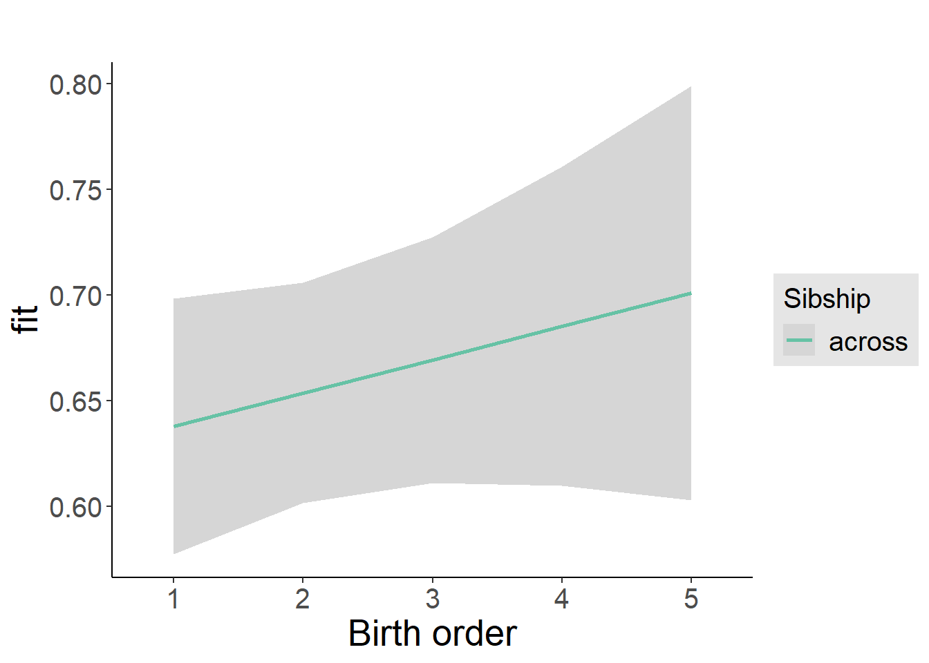
Add Birth Order Factor
Model Summary
m3_birthorder_nonlinear = update(m1_covariates_only, formula = . ~ . + birth_order_nonlinear)
tidy(m3_birthorder_nonlinear, conf.int = T, conf.level = 0.995)| effect | group | term | estimate | std.error | statistic | df | p.value | conf.low | conf.high |
|---|---|---|---|---|---|---|---|---|---|
| fixed | NA | (Intercept) | -7.348 | 0.3826 | -19.21 | 4104 | 8.7e-79 | -8.422 | -6.274 |
| fixed | NA | poly(age, 3, raw = TRUE)1 | 0.7848 | 0.0447 | 17.56 | 4102 | 1.378e-66 | 0.6593 | 0.9103 |
| fixed | NA | poly(age, 3, raw = TRUE)2 | -0.02463 | 0.001652 | -14.91 | 4116 | 5.577e-49 | -0.02926 | -0.01999 |
| fixed | NA | poly(age, 3, raw = TRUE)3 | 0.0002485 | 0.00001941 | 12.8 | 4136 | 7.681e-37 | 0.000194 | 0.000303 |
| fixed | NA | male | -0.07917 | 0.0202 | -3.919 | 3714 | 0.00009067 | -0.1359 | -0.02246 |
| fixed | NA | sibling_count3 | 0.02899 | 0.0338 | 0.8576 | 3381 | 0.3912 | -0.06589 | 0.1239 |
| fixed | NA | sibling_count4 | -0.05305 | 0.03745 | -1.416 | 3325 | 0.1567 | -0.1582 | 0.05208 |
| fixed | NA | sibling_count5 | -0.1425 | 0.04267 | -3.34 | 3354 | 0.0008465 | -0.2623 | -0.02275 |
| fixed | NA | birth_order_nonlinear2 | -0.04527 | 0.02298 | -1.97 | 3116 | 0.04892 | -0.1098 | 0.01923 |
| fixed | NA | birth_order_nonlinear3 | -0.001966 | 0.02937 | -0.06694 | 3306 | 0.9466 | -0.0844 | 0.08046 |
| fixed | NA | birth_order_nonlinear4 | 0.05123 | 0.03947 | 1.298 | 3471 | 0.1944 | -0.05956 | 0.162 |
| fixed | NA | birth_order_nonlinear5 | 0.1288 | 0.05716 | 2.254 | 3230 | 0.02426 | -0.0316 | 0.2893 |
| ran_pars | mother_pidlink | sd__(Intercept) | 0.4974 | NA | NA | NA | NA | NA | NA |
| ran_pars | Residual | sd__Observation | 0.5311 | NA | NA | NA | NA | NA | NA |
Coefficient Plot
plot_birthorder(m3_birthorder_nonlinear, separate = FALSE)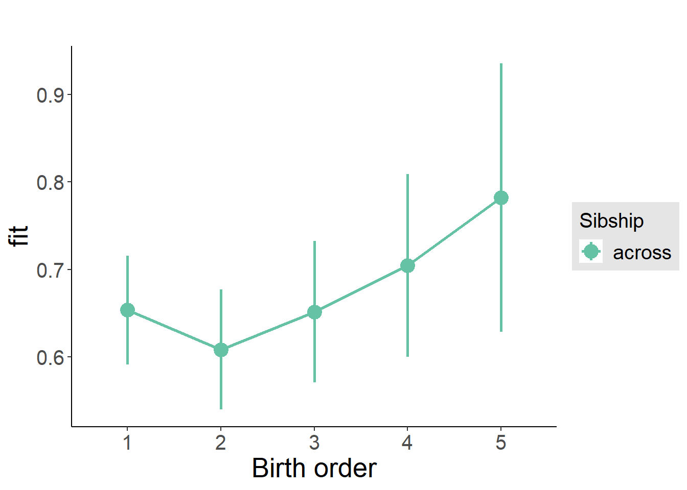
Add Interaction
Model Summary
m4_interaction = update(m3_birthorder_nonlinear, formula = . ~ . - birth_order_nonlinear - sibling_count + count_birth_order)
tidy(m4_interaction, conf.int = T, conf.level = 0.995)| effect | group | term | estimate | std.error | statistic | df | p.value | conf.low | conf.high |
|---|---|---|---|---|---|---|---|---|---|
| fixed | NA | (Intercept) | -7.338 | 0.3831 | -19.16 | 4104 | 2.067e-78 | -8.413 | -6.263 |
| fixed | NA | poly(age, 3, raw = TRUE)1 | 0.7836 | 0.04473 | 17.52 | 4098 | 2.632e-66 | 0.658 | 0.9091 |
| fixed | NA | poly(age, 3, raw = TRUE)2 | -0.02458 | 0.001653 | -14.87 | 4113 | 9.562e-49 | -0.02922 | -0.01994 |
| fixed | NA | poly(age, 3, raw = TRUE)3 | 0.0002481 | 0.00001943 | 12.77 | 4133 | 1.201e-36 | 0.0001935 | 0.0003026 |
| fixed | NA | male | -0.07969 | 0.02023 | -3.94 | 3711 | 0.00008297 | -0.1365 | -0.02292 |
| fixed | NA | count_birth_order2/2 | -0.0407 | 0.04206 | -0.9676 | 3409 | 0.3333 | -0.1588 | 0.07737 |
| fixed | NA | count_birth_order1/3 | 0.04937 | 0.04047 | 1.22 | 4235 | 0.2226 | -0.06424 | 0.163 |
| fixed | NA | count_birth_order2/3 | -0.05495 | 0.04351 | -1.263 | 4324 | 0.2067 | -0.1771 | 0.0672 |
| fixed | NA | count_birth_order3/3 | 0.04642 | 0.048 | 0.9671 | 4326 | 0.3335 | -0.08831 | 0.1811 |
| fixed | NA | count_birth_order1/4 | -0.0827 | 0.0474 | -1.745 | 4312 | 0.08112 | -0.2158 | 0.05036 |
| fixed | NA | count_birth_order2/4 | -0.05819 | 0.04774 | -1.219 | 4332 | 0.223 | -0.1922 | 0.07582 |
| fixed | NA | count_birth_order3/4 | -0.06819 | 0.05154 | -1.323 | 4273 | 0.1858 | -0.2129 | 0.07647 |
| fixed | NA | count_birth_order4/4 | 0.009902 | 0.0533 | 0.1858 | 4280 | 0.8526 | -0.1397 | 0.1595 |
| fixed | NA | count_birth_order1/5 | -0.1378 | 0.05614 | -2.454 | 4331 | 0.01415 | -0.2954 | 0.0198 |
| fixed | NA | count_birth_order2/5 | -0.1687 | 0.05896 | -2.862 | 4242 | 0.004229 | -0.3342 | -0.003246 |
| fixed | NA | count_birth_order3/5 | -0.1516 | 0.05762 | -2.631 | 4242 | 0.00855 | -0.3133 | 0.01016 |
| fixed | NA | count_birth_order4/5 | -0.103 | 0.05956 | -1.729 | 4195 | 0.08386 | -0.2702 | 0.0642 |
| fixed | NA | count_birth_order5/5 | -0.01275 | 0.0593 | -0.215 | 4208 | 0.8298 | -0.1792 | 0.1537 |
| ran_pars | mother_pidlink | sd__(Intercept) | 0.4966 | NA | NA | NA | NA | NA | NA |
| ran_pars | Residual | sd__Observation | 0.5316 | NA | NA | NA | NA | NA | NA |
Coefficient Plot
plot_birthorder(m4_interaction)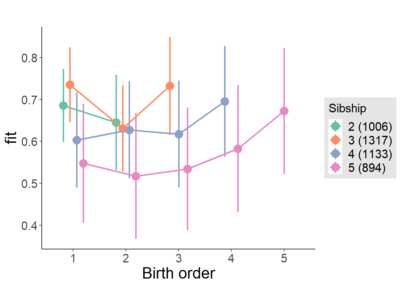
Model Comparison
###### Model 1 - Model 2
anova(m1_covariates_only, m2_birthorder_linear, m3_birthorder_nonlinear, m4_interaction)## refitting model(s) with ML (instead of REML)| Df | AIC | BIC | logLik | deviance | Chisq | Chi Df | Pr(>Chisq) |
|---|---|---|---|---|---|---|---|
| 10 | 9229 | 9293 | -4605 | 9209 | NA | NA | NA |
| 11 | 9229 | 9299 | -4604 | 9207 | 2.402 | 1 | 0.1212 |
| 14 | 9224 | 9314 | -4598 | 9196 | 10.68 | 3 | 0.01362 |
| 20 | 9231 | 9359 | -4596 | 9191 | 5.325 | 6 | 0.5028 |
Parental full sibling order
outcome_parental_m1 <- update(m2_birthorder_linear, data = birthorder %>%
mutate(sibling_count = sibling_count_genes_factor,
birth_order_nonlinear = birthorder_genes_factor,
birth_order = birthorder_genes,
count_birth_order = count_birthorder_genes
) %>%
filter(sibling_count != "1"))
compare_models_markdown(outcome_parental_m1)Basic Model
Model Summary
m1_covariates_only <- update(m2_birthorder_linear, formula = . ~ . - birth_order)
tidy(m1_covariates_only, conf.int = T, conf.level = 0.995)| effect | group | term | estimate | std.error | statistic | df | p.value | conf.low | conf.high |
|---|---|---|---|---|---|---|---|---|---|
| fixed | NA | (Intercept) | -7.211 | 0.3761 | -19.17 | 4346 | 1.012e-78 | -8.267 | -6.155 |
| fixed | NA | poly(age, 3, raw = TRUE)1 | 0.7701 | 0.04403 | 17.49 | 4353 | 3.069e-66 | 0.6465 | 0.8937 |
| fixed | NA | poly(age, 3, raw = TRUE)2 | -0.02411 | 0.001629 | -14.8 | 4371 | 2.25e-48 | -0.02868 | -0.01953 |
| fixed | NA | poly(age, 3, raw = TRUE)3 | 0.0002426 | 0.00001917 | 12.65 | 4396 | 4.612e-36 | 0.0001888 | 0.0002964 |
| fixed | NA | male | -0.08855 | 0.01965 | -4.507 | 3983 | 0.000006772 | -0.1437 | -0.0334 |
| fixed | NA | sibling_count3 | 0.004782 | 0.03063 | 0.1561 | 3477 | 0.876 | -0.0812 | 0.09076 |
| fixed | NA | sibling_count4 | -0.07132 | 0.03382 | -2.109 | 3327 | 0.03505 | -0.1663 | 0.02362 |
| fixed | NA | sibling_count5 | -0.1659 | 0.04076 | -4.07 | 3144 | 0.00004825 | -0.2803 | -0.05147 |
| ran_pars | mother_pidlink | sd__(Intercept) | 0.5046 | NA | NA | NA | NA | NA | NA |
| ran_pars | Residual | sd__Observation | 0.5357 | NA | NA | NA | NA | NA | NA |
Coefficient Plot
plot(allEffects(m1_covariates_only, confidence.level = 0.995))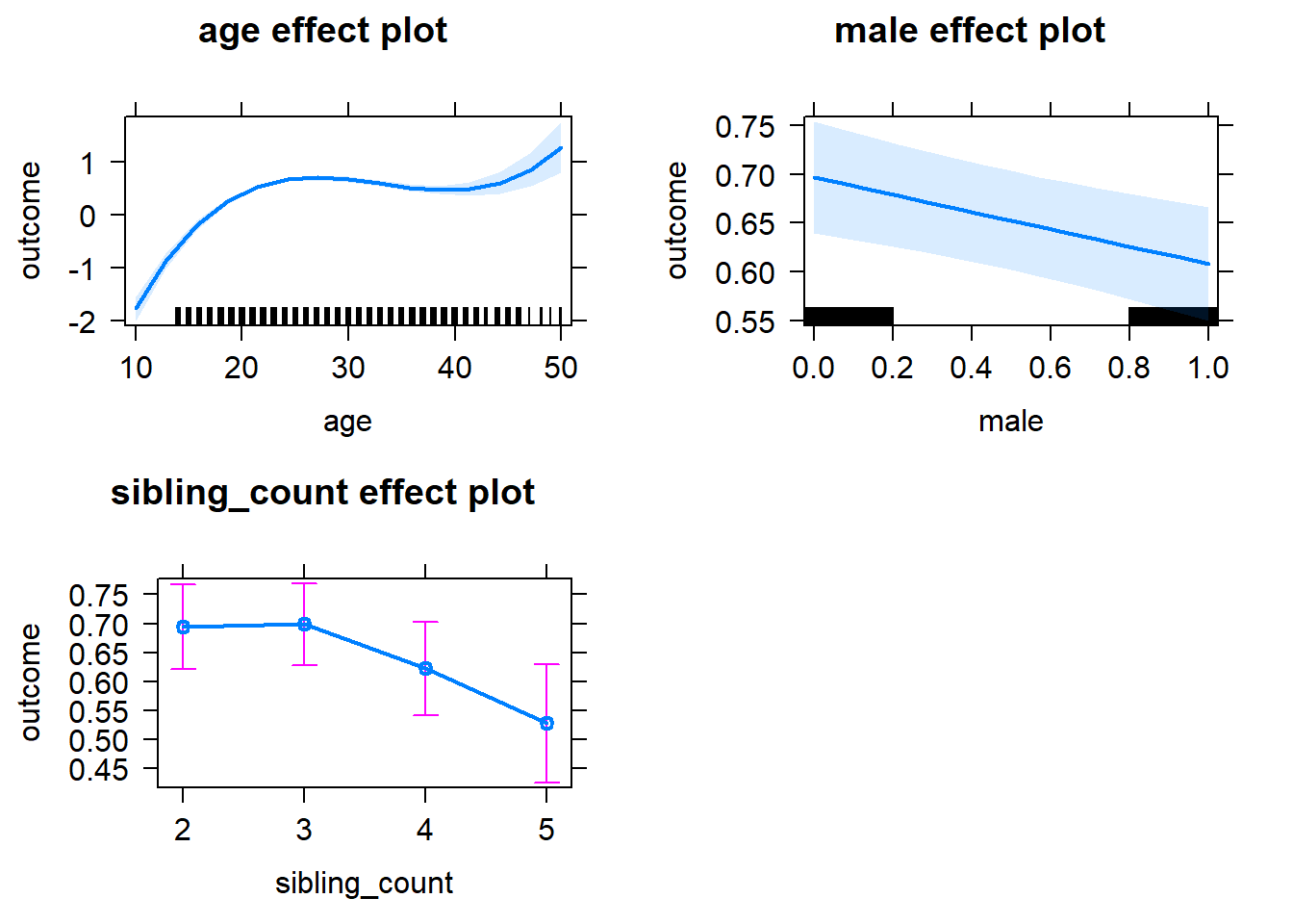
Add Birth Order Linear
Model Summary
tidy(m2_birthorder_linear, conf.int = T, conf.level = 0.995)| effect | group | term | estimate | std.error | statistic | df | p.value | conf.low | conf.high |
|---|---|---|---|---|---|---|---|---|---|
| fixed | NA | (Intercept) | -7.251 | 0.3766 | -19.25 | 4355 | 2.351e-79 | -8.308 | -6.194 |
| fixed | NA | birth_order | 0.01979 | 0.01028 | 1.925 | 4008 | 0.0543 | -0.009067 | 0.04864 |
| fixed | NA | poly(age, 3, raw = TRUE)1 | 0.7713 | 0.04403 | 17.52 | 4354 | 1.88e-66 | 0.6477 | 0.8949 |
| fixed | NA | poly(age, 3, raw = TRUE)2 | -0.02415 | 0.001629 | -14.83 | 4371 | 1.438e-48 | -0.02873 | -0.01958 |
| fixed | NA | poly(age, 3, raw = TRUE)3 | 0.0002436 | 0.00001918 | 12.7 | 4395 | 2.498e-36 | 0.0001898 | 0.0002974 |
| fixed | NA | male | -0.08892 | 0.01965 | -4.526 | 3983 | 0.000006179 | -0.1441 | -0.03378 |
| fixed | NA | sibling_count3 | -0.005083 | 0.03104 | -0.1637 | 3517 | 0.8699 | -0.09222 | 0.08206 |
| fixed | NA | sibling_count4 | -0.09382 | 0.03577 | -2.623 | 3490 | 0.008759 | -0.1942 | 0.00659 |
| fixed | NA | sibling_count5 | -0.2016 | 0.04476 | -4.503 | 3474 | 0.000006919 | -0.3272 | -0.07592 |
| ran_pars | mother_pidlink | sd__(Intercept) | 0.5042 | NA | NA | NA | NA | NA | NA |
| ran_pars | Residual | sd__Observation | 0.5357 | NA | NA | NA | NA | NA | NA |
Coefficient Plot
plot_birthorder2(m2_birthorder_linear, separate = FALSE)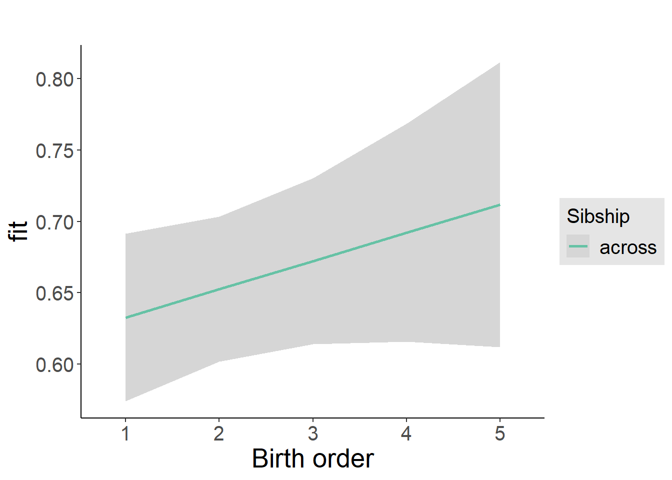
Add Birth Order Factor
Model Summary
m3_birthorder_nonlinear = update(m1_covariates_only, formula = . ~ . + birth_order_nonlinear)
tidy(m3_birthorder_nonlinear, conf.int = T, conf.level = 0.995)| effect | group | term | estimate | std.error | statistic | df | p.value | conf.low | conf.high |
|---|---|---|---|---|---|---|---|---|---|
| fixed | NA | (Intercept) | -7.088 | 0.3774 | -18.78 | 4388 | 9.403e-76 | -8.148 | -6.029 |
| fixed | NA | poly(age, 3, raw = TRUE)1 | 0.758 | 0.04411 | 17.19 | 4382 | 4.112e-64 | 0.6342 | 0.8818 |
| fixed | NA | poly(age, 3, raw = TRUE)2 | -0.0237 | 0.001631 | -14.53 | 4392 | 9.504e-47 | -0.02828 | -0.01912 |
| fixed | NA | poly(age, 3, raw = TRUE)3 | 0.0002388 | 0.00001919 | 12.45 | 4409 | 5.608e-35 | 0.000185 | 0.0002927 |
| fixed | NA | male | -0.08975 | 0.01961 | -4.576 | 3976 | 0.000004884 | -0.1448 | -0.0347 |
| fixed | NA | sibling_count3 | -0.003601 | 0.03133 | -0.1149 | 3606 | 0.9085 | -0.09155 | 0.08435 |
| fixed | NA | sibling_count4 | -0.09878 | 0.03609 | -2.737 | 3569 | 0.006222 | -0.2001 | 0.002511 |
| fixed | NA | sibling_count5 | -0.2281 | 0.04534 | -5.031 | 3584 | 0.000000511 | -0.3554 | -0.1008 |
| fixed | NA | birth_order_nonlinear2 | -0.05814 | 0.02193 | -2.651 | 3272 | 0.008053 | -0.1197 | 0.003411 |
| fixed | NA | birth_order_nonlinear3 | 0.02339 | 0.02839 | 0.8236 | 3475 | 0.4102 | -0.05632 | 0.1031 |
| fixed | NA | birth_order_nonlinear4 | 0.07316 | 0.03958 | 1.848 | 3628 | 0.06464 | -0.03795 | 0.1843 |
| fixed | NA | birth_order_nonlinear5 | 0.1492 | 0.06428 | 2.321 | 3359 | 0.02036 | -0.03126 | 0.3296 |
| ran_pars | mother_pidlink | sd__(Intercept) | 0.5045 | NA | NA | NA | NA | NA | NA |
| ran_pars | Residual | sd__Observation | 0.5343 | NA | NA | NA | NA | NA | NA |
Coefficient Plot
plot_birthorder(m3_birthorder_nonlinear, separate = FALSE)
Add Interaction
Model Summary
m4_interaction = update(m3_birthorder_nonlinear, formula = . ~ . - birth_order_nonlinear - sibling_count + count_birth_order)
tidy(m4_interaction, conf.int = T, conf.level = 0.995)| effect | group | term | estimate | std.error | statistic | df | p.value | conf.low | conf.high |
|---|---|---|---|---|---|---|---|---|---|
| fixed | NA | (Intercept) | -7.092 | 0.3777 | -18.78 | 4386 | 1.025e-75 | -8.153 | -6.032 |
| fixed | NA | poly(age, 3, raw = TRUE)1 | 0.7573 | 0.04413 | 17.16 | 4376 | 6.335e-64 | 0.6334 | 0.8812 |
| fixed | NA | poly(age, 3, raw = TRUE)2 | -0.02368 | 0.001632 | -14.51 | 4386 | 1.3e-46 | -0.02826 | -0.0191 |
| fixed | NA | poly(age, 3, raw = TRUE)3 | 0.0002387 | 0.0000192 | 12.43 | 4403 | 7.043e-35 | 0.0001848 | 0.0002926 |
| fixed | NA | male | -0.08957 | 0.01963 | -4.563 | 3969 | 0.000005199 | -0.1447 | -0.03447 |
| fixed | NA | count_birth_order2/2 | -0.02367 | 0.03719 | -0.6364 | 3516 | 0.5245 | -0.1281 | 0.08073 |
| fixed | NA | count_birth_order1/3 | 0.02922 | 0.03725 | 0.7845 | 4537 | 0.4328 | -0.07534 | 0.1338 |
| fixed | NA | count_birth_order2/3 | -0.06772 | 0.04039 | -1.676 | 4648 | 0.09371 | -0.1811 | 0.04566 |
| fixed | NA | count_birth_order3/3 | 0.0106 | 0.04389 | 0.2416 | 4641 | 0.8091 | -0.1126 | 0.1338 |
| fixed | NA | count_birth_order1/4 | -0.1006 | 0.04571 | -2.201 | 4642 | 0.0278 | -0.2289 | 0.02771 |
| fixed | NA | count_birth_order2/4 | -0.1596 | 0.0464 | -3.439 | 4646 | 0.00059 | -0.2898 | -0.0293 |
| fixed | NA | count_birth_order3/4 | -0.04408 | 0.04822 | -0.9142 | 4595 | 0.3607 | -0.1794 | 0.09128 |
| fixed | NA | count_birth_order4/4 | 0.001783 | 0.05062 | 0.03522 | 4572 | 0.9719 | -0.1403 | 0.1439 |
| fixed | NA | count_birth_order1/5 | -0.2226 | 0.06176 | -3.605 | 4639 | 0.0003153 | -0.396 | -0.04929 |
| fixed | NA | count_birth_order2/5 | -0.2492 | 0.06664 | -3.739 | 4452 | 0.0001868 | -0.4363 | -0.06213 |
| fixed | NA | count_birth_order3/5 | -0.1838 | 0.06317 | -2.909 | 4508 | 0.003646 | -0.3611 | -0.006428 |
| fixed | NA | count_birth_order4/5 | -0.1665 | 0.06175 | -2.697 | 4554 | 0.007031 | -0.3399 | 0.006819 |
| fixed | NA | count_birth_order5/5 | -0.06767 | 0.06494 | -1.042 | 4480 | 0.2974 | -0.2499 | 0.1146 |
| ran_pars | mother_pidlink | sd__(Intercept) | 0.5041 | NA | NA | NA | NA | NA | NA |
| ran_pars | Residual | sd__Observation | 0.5347 | NA | NA | NA | NA | NA | NA |
Coefficient Plot
plot_birthorder(m4_interaction)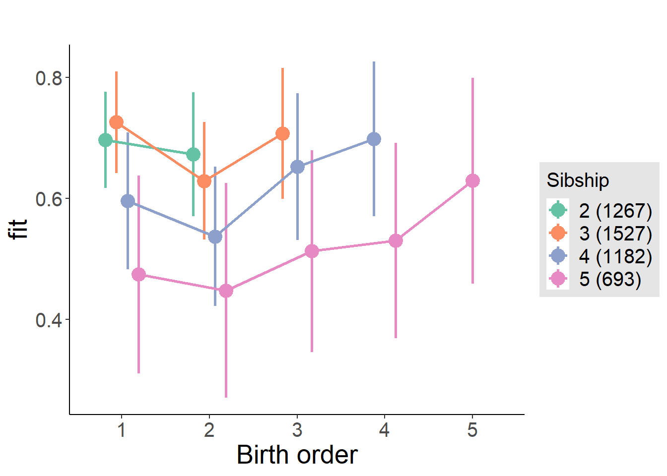
Model Comparison
###### Model 1 - Model 2
anova(m1_covariates_only, m2_birthorder_linear, m3_birthorder_nonlinear, m4_interaction)## refitting model(s) with ML (instead of REML)| Df | AIC | BIC | logLik | deviance | Chisq | Chi Df | Pr(>Chisq) |
|---|---|---|---|---|---|---|---|
| 10 | 9979 | 10043 | -4979 | 9959 | NA | NA | NA |
| 11 | 9977 | 10048 | -4978 | 9955 | 3.712 | 1 | 0.05403 |
| 14 | 9966 | 10057 | -4969 | 9938 | 16.72 | 3 | 0.0008055 |
| 20 | 9975 | 10104 | -4967 | 9935 | 3.655 | 6 | 0.7233 |
Compare birth order specifications
library(coefplot)
multiplot(outcome_naive_m1, outcome_preg_m1, outcome_uterus_m1, outcome_parental_m1, dodgeHeight = 0.6,
intercept = FALSE)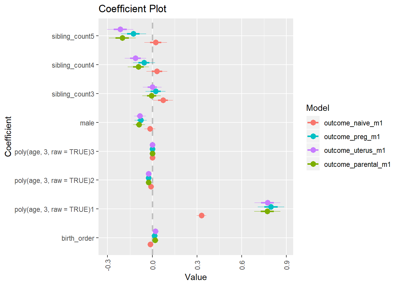
Elementary missed
birthorder <- birthorder %>% mutate(outcome = Elementary_missed)
model = lmer(outcome ~ birth_order + poly(age, 3, raw = TRUE) + male + sibling_count + (1 | mother_pidlink),
data = birthorder)## boundary (singular) fit: see ?isSingularcompare_birthorder_specs(model)Naive birth order
outcome_naive_m1 <- update(m2_birthorder_linear, data = birthorder %>%
mutate(sibling_count = sibling_count_naive_factor,
birth_order_nonlinear = birthorder_naive_factor,
birth_order = birthorder_naive,
count_birth_order = count_birthorder_naive) %>%
filter(sibling_count != "1"))## boundary (singular) fit: see ?isSingularcompare_models_markdown(outcome_naive_m1)Basic Model
Model Summary
m1_covariates_only <- update(m2_birthorder_linear, formula = . ~ . - birth_order)## boundary (singular) fit: see ?isSingulartidy(m1_covariates_only, conf.int = T, conf.level = 0.995)| effect | group | term | estimate | std.error | statistic | df | p.value | conf.low | conf.high |
|---|---|---|---|---|---|---|---|---|---|
| fixed | NA | (Intercept) | -0.06405 | 0.08209 | -0.7802 | 4285 | 0.4353 | -0.2945 | 0.1664 |
| fixed | NA | poly(age, 3, raw = TRUE)1 | 0.008914 | 0.009546 | 0.9338 | 4285 | 0.3505 | -0.01788 | 0.03571 |
| fixed | NA | poly(age, 3, raw = TRUE)2 | -0.0002855 | 0.0003483 | -0.8198 | 4285 | 0.4124 | -0.001263 | 0.0006922 |
| fixed | NA | poly(age, 3, raw = TRUE)3 | 0.000002916 | 0.000003985 | 0.7317 | 4285 | 0.4644 | -0.00000827 | 0.0000141 |
| fixed | NA | male | 0.01113 | 0.004914 | 2.264 | 4285 | 0.02362 | -0.002669 | 0.02492 |
| fixed | NA | sibling_count3 | -0.004754 | 0.006787 | -0.7006 | 4285 | 0.4836 | -0.0238 | 0.0143 |
| fixed | NA | sibling_count4 | 0.002237 | 0.006986 | 0.3202 | 4285 | 0.7489 | -0.01737 | 0.02185 |
| fixed | NA | sibling_count5 | 0.0006969 | 0.007226 | 0.09644 | 4285 | 0.9232 | -0.01959 | 0.02098 |
| ran_pars | mother_pidlink | sd__(Intercept) | 0 | NA | NA | NA | NA | NA | NA |
| ran_pars | Residual | sd__Observation | 0.1608 | NA | NA | NA | NA | NA | NA |
Coefficient Plot
plot(allEffects(m1_covariates_only, confidence.level = 0.995))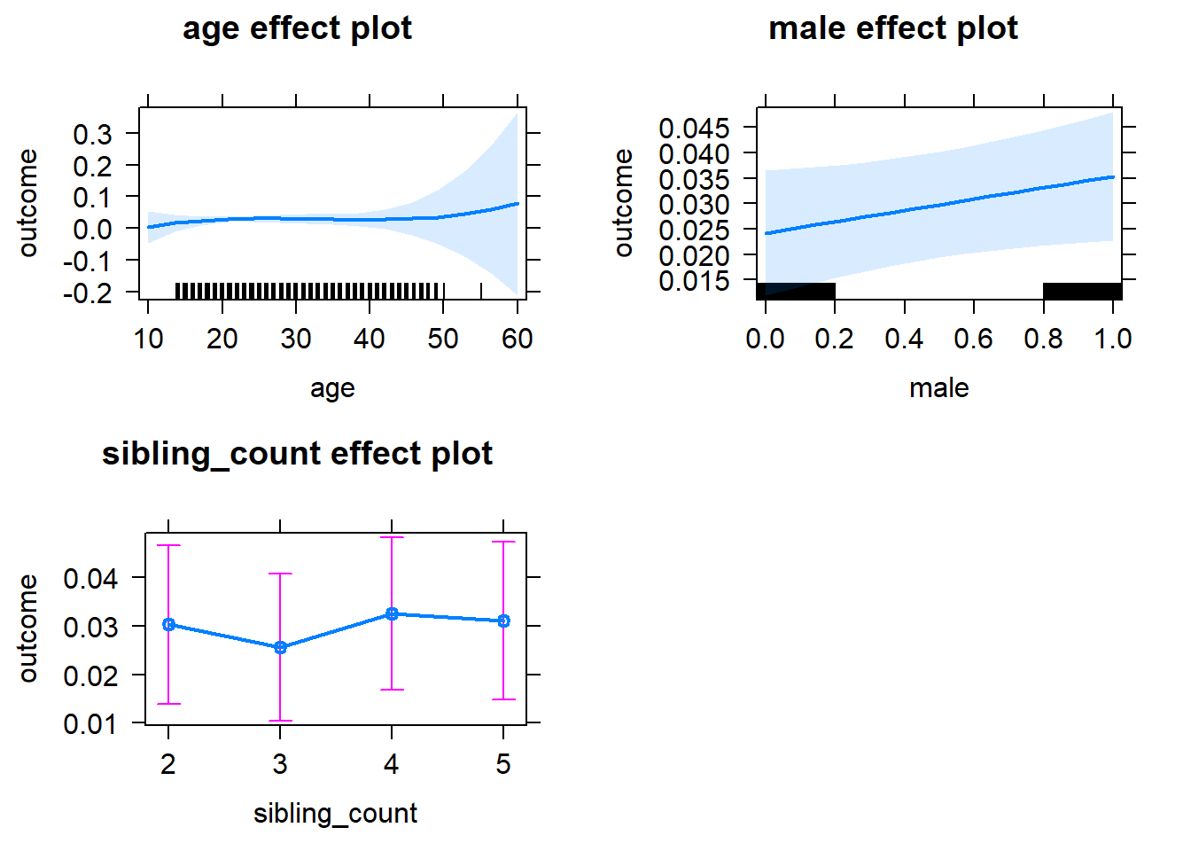
Add Birth Order Linear
Model Summary
tidy(m2_birthorder_linear, conf.int = T, conf.level = 0.995)| effect | group | term | estimate | std.error | statistic | df | p.value | conf.low | conf.high |
|---|---|---|---|---|---|---|---|---|---|
| fixed | NA | (Intercept) | -0.06261 | 0.08232 | -0.7606 | 4284 | 0.4469 | -0.2937 | 0.1685 |
| fixed | NA | birth_order | -0.0005888 | 0.002461 | -0.2392 | 4284 | 0.8109 | -0.007497 | 0.00632 |
| fixed | NA | poly(age, 3, raw = TRUE)1 | 0.008825 | 0.009555 | 0.9237 | 4284 | 0.3557 | -0.01799 | 0.03565 |
| fixed | NA | poly(age, 3, raw = TRUE)2 | -0.0002818 | 0.0003487 | -0.8083 | 4284 | 0.419 | -0.001261 | 0.000697 |
| fixed | NA | poly(age, 3, raw = TRUE)3 | 0.00000287 | 0.00000399 | 0.7193 | 4284 | 0.472 | -0.00000833 | 0.00001407 |
| fixed | NA | male | 0.01114 | 0.004915 | 2.266 | 4284 | 0.02349 | -0.002658 | 0.02494 |
| fixed | NA | sibling_count3 | -0.004516 | 0.00686 | -0.6582 | 4284 | 0.5104 | -0.02377 | 0.01474 |
| fixed | NA | sibling_count4 | 0.002809 | 0.007384 | 0.3803 | 4284 | 0.7037 | -0.01792 | 0.02354 |
| fixed | NA | sibling_count5 | 0.001613 | 0.008178 | 0.1972 | 4284 | 0.8437 | -0.02134 | 0.02457 |
| ran_pars | mother_pidlink | sd__(Intercept) | 0.0000000003416 | NA | NA | NA | NA | NA | NA |
| ran_pars | Residual | sd__Observation | 0.1608 | NA | NA | NA | NA | NA | NA |
Coefficient Plot
plot_birthorder2(m2_birthorder_linear, separate = FALSE)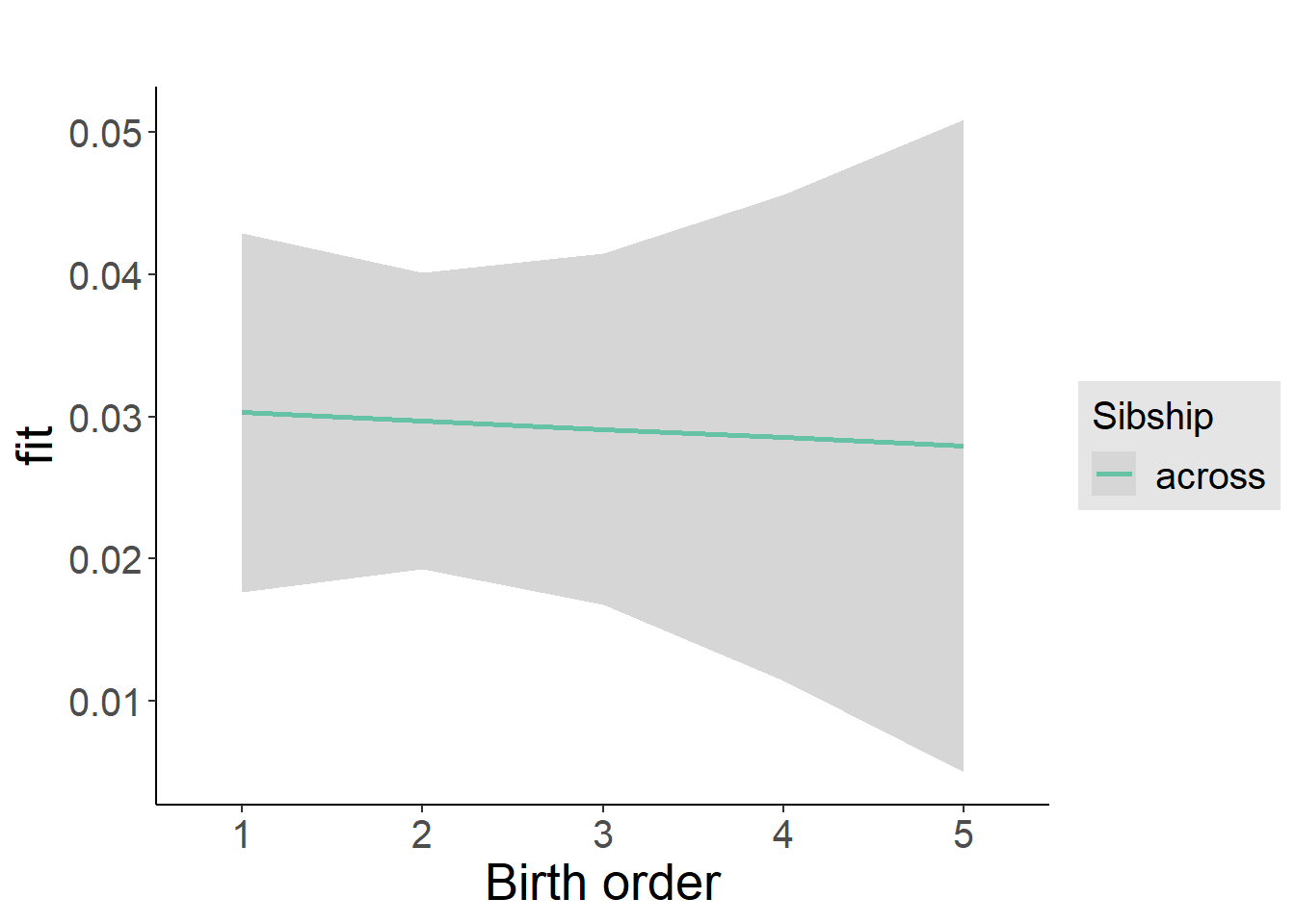
Add Birth Order Factor
Model Summary
m3_birthorder_nonlinear = update(m1_covariates_only, formula = . ~ . + birth_order_nonlinear)## boundary (singular) fit: see ?isSingulartidy(m3_birthorder_nonlinear, conf.int = T, conf.level = 0.995)| effect | group | term | estimate | std.error | statistic | df | p.value | conf.low | conf.high |
|---|---|---|---|---|---|---|---|---|---|
| fixed | NA | (Intercept) | -0.07008 | 0.08235 | -0.851 | 4281 | 0.3948 | -0.3012 | 0.1611 |
| fixed | NA | poly(age, 3, raw = TRUE)1 | 0.009333 | 0.009563 | 0.976 | 4281 | 0.3291 | -0.01751 | 0.03618 |
| fixed | NA | poly(age, 3, raw = TRUE)2 | -0.0002999 | 0.000349 | -0.8595 | 4281 | 0.3901 | -0.00128 | 0.0006797 |
| fixed | NA | poly(age, 3, raw = TRUE)3 | 0.000003062 | 0.000003993 | 0.7668 | 4281 | 0.4432 | -0.000008146 | 0.00001427 |
| fixed | NA | male | 0.01123 | 0.004916 | 2.284 | 4281 | 0.0224 | -0.00257 | 0.02503 |
| fixed | NA | sibling_count3 | -0.003716 | 0.006971 | -0.533 | 4281 | 0.5941 | -0.02328 | 0.01585 |
| fixed | NA | sibling_count4 | 0.003706 | 0.007536 | 0.4918 | 4281 | 0.6229 | -0.01745 | 0.02486 |
| fixed | NA | sibling_count5 | 0.003001 | 0.008267 | 0.363 | 4281 | 0.7166 | -0.02021 | 0.02621 |
| fixed | NA | birth_order_nonlinear2 | 0.006739 | 0.005987 | 1.126 | 4281 | 0.2604 | -0.01007 | 0.02354 |
| fixed | NA | birth_order_nonlinear3 | -0.004113 | 0.007625 | -0.5394 | 4281 | 0.5897 | -0.02552 | 0.01729 |
| fixed | NA | birth_order_nonlinear4 | -0.0003551 | 0.009867 | -0.03599 | 4281 | 0.9713 | -0.02805 | 0.02734 |
| fixed | NA | birth_order_nonlinear5 | -0.001871 | 0.01371 | -0.1364 | 4281 | 0.8915 | -0.04037 | 0.03663 |
| ran_pars | mother_pidlink | sd__(Intercept) | 0 | NA | NA | NA | NA | NA | NA |
| ran_pars | Residual | sd__Observation | 0.1608 | NA | NA | NA | NA | NA | NA |
Coefficient Plot
plot_birthorder(m3_birthorder_nonlinear, separate = FALSE)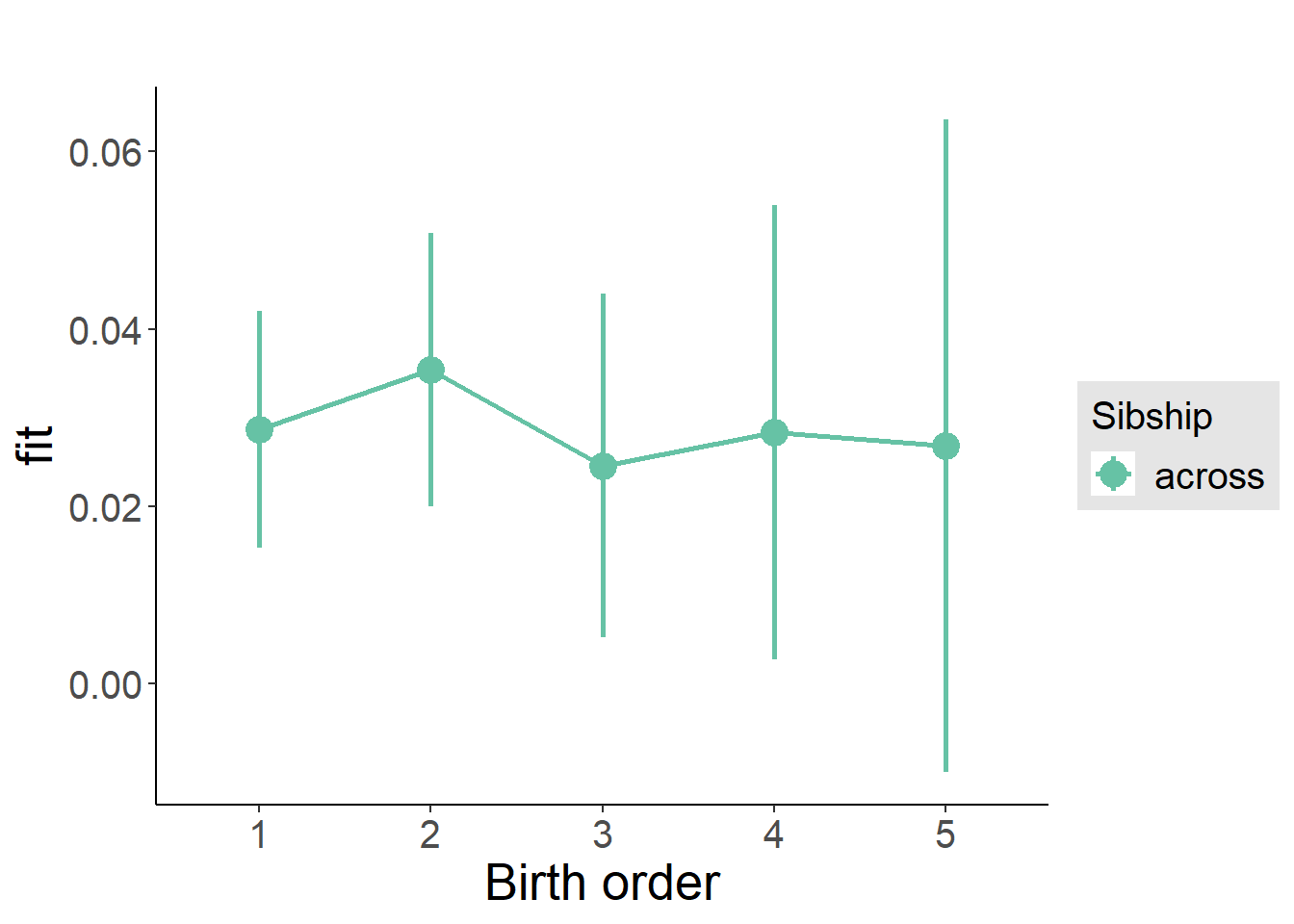
Add Interaction
Model Summary
m4_interaction = update(m3_birthorder_nonlinear, formula = . ~ . - birth_order_nonlinear - sibling_count + count_birth_order)## boundary (singular) fit: see ?isSingulartidy(m4_interaction, conf.int = T, conf.level = 0.995)| effect | group | term | estimate | std.error | statistic | df | p.value | conf.low | conf.high |
|---|---|---|---|---|---|---|---|---|---|
| fixed | NA | (Intercept) | -0.07301 | 0.08244 | -0.8856 | 4275 | 0.3759 | -0.3044 | 0.1584 |
| fixed | NA | poly(age, 3, raw = TRUE)1 | 0.00955 | 0.009567 | 0.9983 | 4275 | 0.3182 | -0.0173 | 0.0364 |
| fixed | NA | poly(age, 3, raw = TRUE)2 | -0.0003061 | 0.0003491 | -0.8767 | 4275 | 0.3807 | -0.001286 | 0.000674 |
| fixed | NA | poly(age, 3, raw = TRUE)3 | 0.000003113 | 0.000003995 | 0.7792 | 4275 | 0.4359 | -0.000008101 | 0.00001433 |
| fixed | NA | male | 0.0113 | 0.004918 | 2.298 | 4275 | 0.02158 | -0.002501 | 0.02511 |
| fixed | NA | count_birth_order2/2 | 0.008721 | 0.01044 | 0.8353 | 4275 | 0.4036 | -0.02058 | 0.03803 |
| fixed | NA | count_birth_order1/3 | 0.0009068 | 0.009166 | 0.09894 | 4275 | 0.9212 | -0.02482 | 0.02664 |
| fixed | NA | count_birth_order2/3 | -0.003208 | 0.0102 | -0.3147 | 4275 | 0.753 | -0.03183 | 0.02541 |
| fixed | NA | count_birth_order3/3 | -0.005225 | 0.01175 | -0.4447 | 4275 | 0.6566 | -0.0382 | 0.02775 |
| fixed | NA | count_birth_order1/4 | 0.006251 | 0.01083 | 0.5774 | 4275 | 0.5637 | -0.02414 | 0.03664 |
| fixed | NA | count_birth_order2/4 | 0.01993 | 0.01121 | 1.778 | 4275 | 0.07552 | -0.01154 | 0.05141 |
| fixed | NA | count_birth_order3/4 | -0.01207 | 0.01212 | -0.9959 | 4275 | 0.3193 | -0.04608 | 0.02195 |
| fixed | NA | count_birth_order4/4 | 0.00277 | 0.01256 | 0.2204 | 4275 | 0.8255 | -0.0325 | 0.03804 |
| fixed | NA | count_birth_order1/5 | -0.006998 | 0.01248 | -0.5606 | 4275 | 0.5751 | -0.04204 | 0.02804 |
| fixed | NA | count_birth_order2/5 | 0.008497 | 0.01338 | 0.6352 | 4275 | 0.5254 | -0.02905 | 0.04605 |
| fixed | NA | count_birth_order3/5 | 0.0122 | 0.01313 | 0.9291 | 4275 | 0.3529 | -0.02465 | 0.04904 |
| fixed | NA | count_birth_order4/5 | 0.004902 | 0.01388 | 0.3531 | 4275 | 0.724 | -0.03407 | 0.04387 |
| fixed | NA | count_birth_order5/5 | 0.001783 | 0.01328 | 0.1343 | 4275 | 0.8932 | -0.0355 | 0.03907 |
| ran_pars | mother_pidlink | sd__(Intercept) | 0 | NA | NA | NA | NA | NA | NA |
| ran_pars | Residual | sd__Observation | 0.1608 | NA | NA | NA | NA | NA | NA |
Coefficient Plot
plot_birthorder(m4_interaction)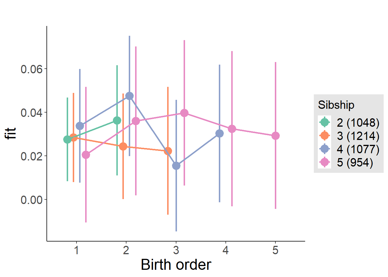
Model Comparison
###### Model 1 - Model 2
anova(m1_covariates_only, m2_birthorder_linear, m3_birthorder_nonlinear, m4_interaction)## refitting model(s) with ML (instead of REML)| Df | AIC | BIC | logLik | deviance | Chisq | Chi Df | Pr(>Chisq) |
|---|---|---|---|---|---|---|---|
| 10 | -3498 | -3435 | 1759 | -3518 | NA | NA | NA |
| 11 | -3496 | -3426 | 1759 | -3518 | 0.05736 | 1 | 0.8107 |
| 14 | -3493 | -3404 | 1760 | -3521 | 2.259 | 3 | 0.5204 |
| 20 | -3486 | -3359 | 1763 | -3526 | 5.705 | 6 | 0.457 |
Maternal birth order
outcome_uterus_m1 <- update(m2_birthorder_linear, data = birthorder %>%
mutate(sibling_count = sibling_count_uterus_alive_factor,
birth_order_nonlinear = birthorder_uterus_alive_factor,
birth_order = birthorder_uterus_alive,
count_birth_order = count_birthorder_uterus_alive) %>%
filter(sibling_count != "1"))## boundary (singular) fit: see ?isSingularcompare_models_markdown(outcome_uterus_m1)Basic Model
Model Summary
m1_covariates_only <- update(m2_birthorder_linear, formula = . ~ . - birth_order)## boundary (singular) fit: see ?isSingulartidy(m1_covariates_only, conf.int = T, conf.level = 0.995)| effect | group | term | estimate | std.error | statistic | df | p.value | conf.low | conf.high |
|---|---|---|---|---|---|---|---|---|---|
| fixed | NA | (Intercept) | -0.1111 | 0.1254 | -0.8862 | 3310 | 0.3756 | -0.463 | 0.2408 |
| fixed | NA | poly(age, 3, raw = TRUE)1 | 0.01595 | 0.01564 | 1.02 | 3310 | 0.3078 | -0.02795 | 0.05985 |
| fixed | NA | poly(age, 3, raw = TRUE)2 | -0.0006233 | 0.0006197 | -1.006 | 3310 | 0.3146 | -0.002363 | 0.001116 |
| fixed | NA | poly(age, 3, raw = TRUE)3 | 0.00000807 | 0.000007777 | 1.038 | 3310 | 0.2995 | -0.00001376 | 0.0000299 |
| fixed | NA | male | 0.009184 | 0.005331 | 1.723 | 3310 | 0.08506 | -0.005782 | 0.02415 |
| fixed | NA | sibling_count3 | -0.003343 | 0.006687 | -0.4999 | 3310 | 0.6172 | -0.02211 | 0.01543 |
| fixed | NA | sibling_count4 | -0.004969 | 0.007465 | -0.6656 | 3310 | 0.5057 | -0.02592 | 0.01599 |
| fixed | NA | sibling_count5 | 0.00186 | 0.00885 | 0.2101 | 3310 | 0.8336 | -0.02298 | 0.0267 |
| ran_pars | mother_pidlink | sd__(Intercept) | 0 | NA | NA | NA | NA | NA | NA |
| ran_pars | Residual | sd__Observation | 0.1534 | NA | NA | NA | NA | NA | NA |
Coefficient Plot
plot(allEffects(m1_covariates_only, confidence.level = 0.995))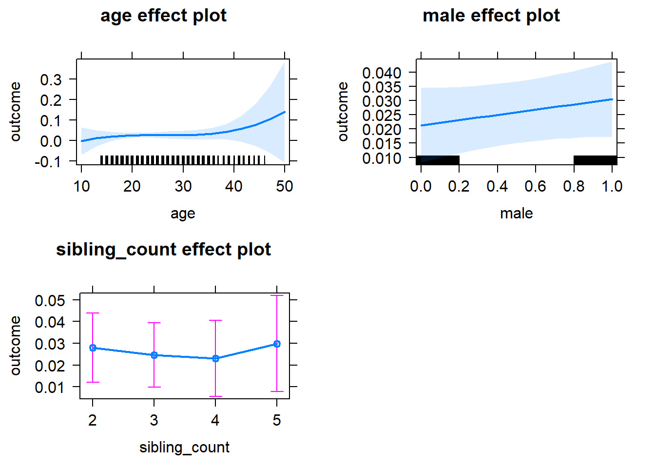
Add Birth Order Linear
Model Summary
tidy(m2_birthorder_linear, conf.int = T, conf.level = 0.995)| effect | group | term | estimate | std.error | statistic | df | p.value | conf.low | conf.high |
|---|---|---|---|---|---|---|---|---|---|
| fixed | NA | (Intercept) | -0.1072 | 0.1255 | -0.8541 | 3309 | 0.3931 | -0.4595 | 0.2451 |
| fixed | NA | birth_order | -0.002006 | 0.002908 | -0.6898 | 3309 | 0.4904 | -0.01017 | 0.006157 |
| fixed | NA | poly(age, 3, raw = TRUE)1 | 0.01578 | 0.01564 | 1.009 | 3309 | 0.3131 | -0.02813 | 0.05969 |
| fixed | NA | poly(age, 3, raw = TRUE)2 | -0.0006157 | 0.0006199 | -0.9934 | 3309 | 0.3206 | -0.002356 | 0.001124 |
| fixed | NA | poly(age, 3, raw = TRUE)3 | 0.000007959 | 0.000007779 | 1.023 | 3309 | 0.3063 | -0.00001388 | 0.0000298 |
| fixed | NA | male | 0.009237 | 0.005332 | 1.732 | 3309 | 0.08333 | -0.005731 | 0.0242 |
| fixed | NA | sibling_count3 | -0.00242 | 0.00682 | -0.3549 | 3309 | 0.7227 | -0.02156 | 0.01672 |
| fixed | NA | sibling_count4 | -0.002807 | 0.008097 | -0.3467 | 3309 | 0.7288 | -0.02554 | 0.01992 |
| fixed | NA | sibling_count5 | 0.005452 | 0.01027 | 0.5309 | 3309 | 0.5955 | -0.02337 | 0.03428 |
| ran_pars | mother_pidlink | sd__(Intercept) | 0 | NA | NA | NA | NA | NA | NA |
| ran_pars | Residual | sd__Observation | 0.1534 | NA | NA | NA | NA | NA | NA |
Coefficient Plot
plot_birthorder2(m2_birthorder_linear, separate = FALSE)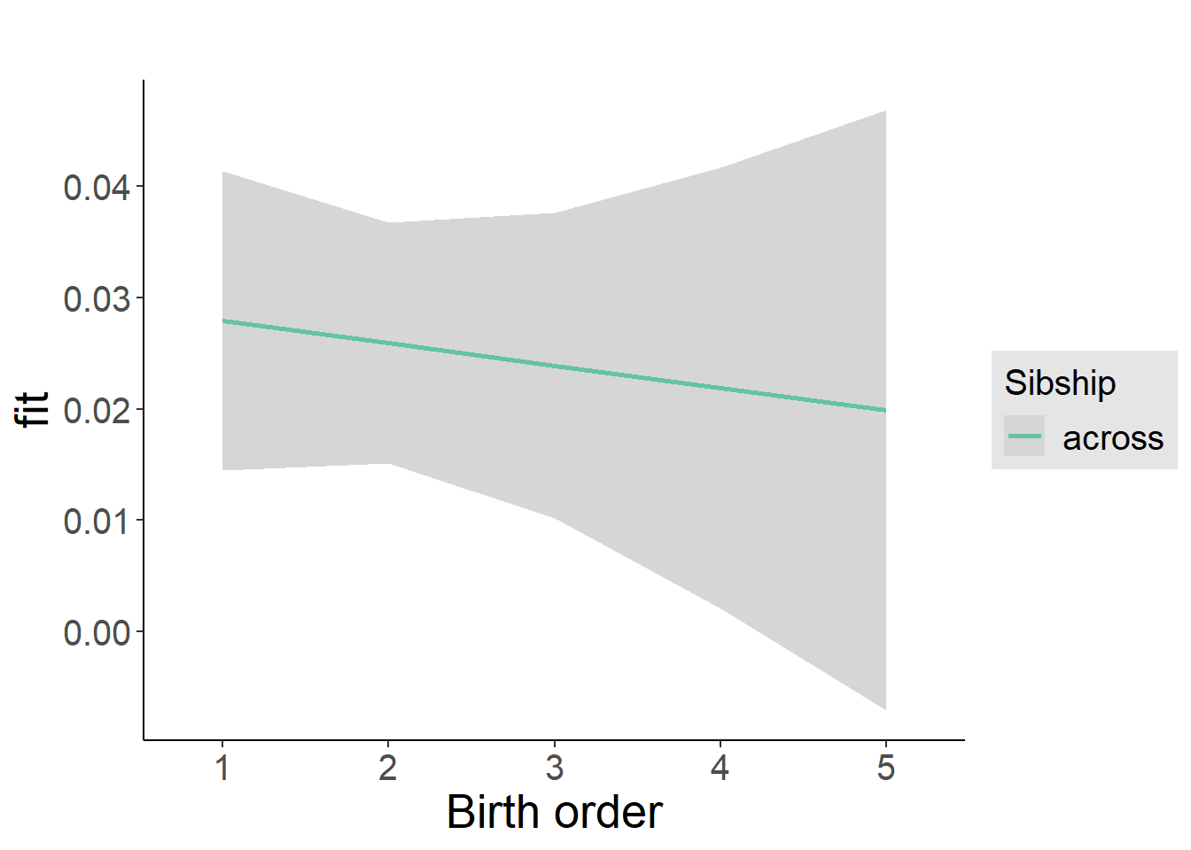
Add Birth Order Factor
Model Summary
m3_birthorder_nonlinear = update(m1_covariates_only, formula = . ~ . + birth_order_nonlinear)## boundary (singular) fit: see ?isSingulartidy(m3_birthorder_nonlinear, conf.int = T, conf.level = 0.995)| effect | group | term | estimate | std.error | statistic | df | p.value | conf.low | conf.high |
|---|---|---|---|---|---|---|---|---|---|
| fixed | NA | (Intercept) | -0.1143 | 0.1256 | -0.91 | 3306 | 0.3629 | -0.4669 | 0.2383 |
| fixed | NA | poly(age, 3, raw = TRUE)1 | 0.01617 | 0.01566 | 1.033 | 3306 | 0.3018 | -0.02778 | 0.06012 |
| fixed | NA | poly(age, 3, raw = TRUE)2 | -0.0006293 | 0.0006204 | -1.014 | 3306 | 0.3105 | -0.002371 | 0.001112 |
| fixed | NA | poly(age, 3, raw = TRUE)3 | 0.000008099 | 0.000007786 | 1.04 | 3306 | 0.2983 | -0.00001376 | 0.00002995 |
| fixed | NA | male | 0.009276 | 0.005335 | 1.739 | 3306 | 0.08221 | -0.005701 | 0.02425 |
| fixed | NA | sibling_count3 | -0.002931 | 0.006964 | -0.4209 | 3306 | 0.6738 | -0.02248 | 0.01662 |
| fixed | NA | sibling_count4 | -0.002306 | 0.008264 | -0.2791 | 3306 | 0.7802 | -0.0255 | 0.02089 |
| fixed | NA | sibling_count5 | 0.00733 | 0.01056 | 0.6944 | 3306 | 0.4875 | -0.0223 | 0.03696 |
| fixed | NA | birth_order_nonlinear2 | 0.003146 | 0.006416 | 0.4903 | 3306 | 0.6239 | -0.01486 | 0.02116 |
| fixed | NA | birth_order_nonlinear3 | -0.001621 | 0.008373 | -0.1936 | 3306 | 0.8465 | -0.02512 | 0.02188 |
| fixed | NA | birth_order_nonlinear4 | -0.008807 | 0.01138 | -0.7736 | 3306 | 0.4392 | -0.04076 | 0.02315 |
| fixed | NA | birth_order_nonlinear5 | -0.01174 | 0.01842 | -0.6372 | 3306 | 0.524 | -0.06344 | 0.03997 |
| ran_pars | mother_pidlink | sd__(Intercept) | 0 | NA | NA | NA | NA | NA | NA |
| ran_pars | Residual | sd__Observation | 0.1535 | NA | NA | NA | NA | NA | NA |
Coefficient Plot
plot_birthorder(m3_birthorder_nonlinear, separate = FALSE)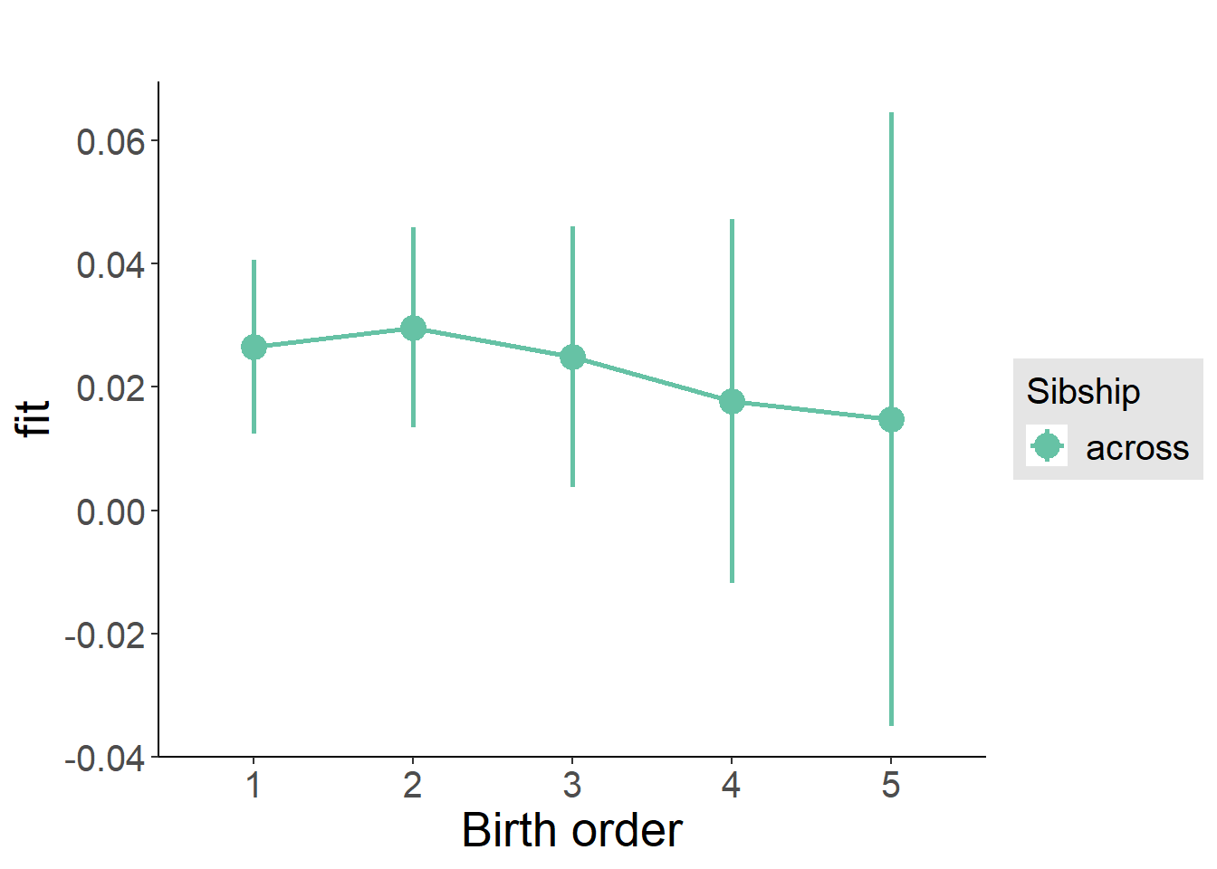
Add Interaction
Model Summary
m4_interaction = update(m3_birthorder_nonlinear, formula = . ~ . - birth_order_nonlinear - sibling_count + count_birth_order)## boundary (singular) fit: see ?isSingulartidy(m4_interaction, conf.int = T, conf.level = 0.995)| effect | group | term | estimate | std.error | statistic | df | p.value | conf.low | conf.high |
|---|---|---|---|---|---|---|---|---|---|
| fixed | NA | (Intercept) | -0.1164 | 0.1257 | -0.9258 | 3300 | 0.3546 | -0.4694 | 0.2365 |
| fixed | NA | poly(age, 3, raw = TRUE)1 | 0.01672 | 0.01567 | 1.067 | 3300 | 0.286 | -0.02727 | 0.06071 |
| fixed | NA | poly(age, 3, raw = TRUE)2 | -0.0006469 | 0.000621 | -1.042 | 3300 | 0.2976 | -0.00239 | 0.001096 |
| fixed | NA | poly(age, 3, raw = TRUE)3 | 0.000008268 | 0.000007793 | 1.061 | 3300 | 0.2888 | -0.00001361 | 0.00003014 |
| fixed | NA | male | 0.009474 | 0.00534 | 1.774 | 3300 | 0.07612 | -0.005515 | 0.02446 |
| fixed | NA | count_birth_order2/2 | -0.006587 | 0.01038 | -0.6348 | 3300 | 0.5256 | -0.03572 | 0.02254 |
| fixed | NA | count_birth_order1/3 | -0.01279 | 0.009121 | -1.402 | 3300 | 0.161 | -0.03839 | 0.01281 |
| fixed | NA | count_birth_order2/3 | 0.001834 | 0.009984 | 0.1837 | 3300 | 0.8543 | -0.02619 | 0.02986 |
| fixed | NA | count_birth_order3/3 | -0.002196 | 0.01117 | -0.1965 | 3300 | 0.8442 | -0.03356 | 0.02917 |
| fixed | NA | count_birth_order1/4 | -0.0005371 | 0.01215 | -0.0442 | 3300 | 0.9647 | -0.03465 | 0.03357 |
| fixed | NA | count_birth_order2/4 | 0.002783 | 0.01259 | 0.221 | 3300 | 0.8251 | -0.03257 | 0.03813 |
| fixed | NA | count_birth_order3/4 | -0.01698 | 0.01326 | -1.281 | 3300 | 0.2004 | -0.05421 | 0.02024 |
| fixed | NA | count_birth_order4/4 | -0.01687 | 0.01311 | -1.287 | 3300 | 0.1982 | -0.05366 | 0.01992 |
| fixed | NA | count_birth_order1/5 | 0.005217 | 0.01765 | 0.2955 | 3300 | 0.7676 | -0.04434 | 0.05477 |
| fixed | NA | count_birth_order2/5 | -0.002252 | 0.01914 | -0.1177 | 3300 | 0.9063 | -0.05599 | 0.05148 |
| fixed | NA | count_birth_order3/5 | 0.004141 | 0.0174 | 0.238 | 3300 | 0.8119 | -0.0447 | 0.05298 |
| fixed | NA | count_birth_order4/5 | -0.0006506 | 0.01636 | -0.03976 | 3300 | 0.9683 | -0.04658 | 0.04528 |
| fixed | NA | count_birth_order5/5 | -0.007705 | 0.0168 | -0.4586 | 3300 | 0.6465 | -0.05486 | 0.03945 |
| ran_pars | mother_pidlink | sd__(Intercept) | 0 | NA | NA | NA | NA | NA | NA |
| ran_pars | Residual | sd__Observation | 0.1535 | NA | NA | NA | NA | NA | NA |
Coefficient Plot
plot_birthorder(m4_interaction)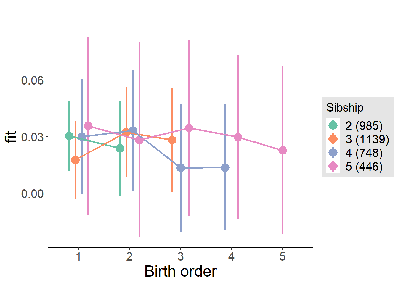
Model Comparison
###### Model 1 - Model 2
anova(m1_covariates_only, m2_birthorder_linear, m3_birthorder_nonlinear, m4_interaction)## refitting model(s) with ML (instead of REML)| Df | AIC | BIC | logLik | deviance | Chisq | Chi Df | Pr(>Chisq) |
|---|---|---|---|---|---|---|---|
| 10 | -3012 | -2951 | 1516 | -3032 | NA | NA | NA |
| 11 | -3011 | -2944 | 1516 | -3033 | 0.477 | 1 | 0.4898 |
| 14 | -3006 | -2920 | 1517 | -3034 | 0.95 | 3 | 0.8133 |
| 20 | -2998 | -2876 | 1519 | -3038 | 4.098 | 6 | 0.6634 |
Maternal pregnancy order
outcome_preg_m1 <- update(m2_birthorder_linear, data = birthorder %>%
mutate(sibling_count = sibling_count_uterus_preg_factor,
birth_order_nonlinear = birthorder_uterus_preg_factor,
birth_order = birthorder_uterus_preg,
count_birth_order = count_birthorder_uterus_preg
) %>%
filter(sibling_count != "1"))## boundary (singular) fit: see ?isSingularcompare_models_markdown(outcome_preg_m1)Basic Model
Model Summary
m1_covariates_only <- update(m2_birthorder_linear, formula = . ~ . - birth_order)## boundary (singular) fit: see ?isSingulartidy(m1_covariates_only, conf.int = T, conf.level = 0.995)| effect | group | term | estimate | std.error | statistic | df | p.value | conf.low | conf.high |
|---|---|---|---|---|---|---|---|---|---|
| fixed | NA | (Intercept) | -0.09555 | 0.1279 | -0.7468 | 3110 | 0.4552 | -0.4547 | 0.2636 |
| fixed | NA | poly(age, 3, raw = TRUE)1 | 0.01352 | 0.01596 | 0.8474 | 3110 | 0.3968 | -0.03127 | 0.05832 |
| fixed | NA | poly(age, 3, raw = TRUE)2 | -0.0005147 | 0.0006321 | -0.8142 | 3110 | 0.4156 | -0.002289 | 0.00126 |
| fixed | NA | poly(age, 3, raw = TRUE)3 | 0.000006592 | 0.000007924 | 0.8319 | 3110 | 0.4055 | -0.00001565 | 0.00002883 |
| fixed | NA | male | 0.009673 | 0.005459 | 1.772 | 3110 | 0.07654 | -0.005652 | 0.025 |
| fixed | NA | sibling_count3 | 0.002693 | 0.00716 | 0.3761 | 3110 | 0.7069 | -0.01741 | 0.02279 |
| fixed | NA | sibling_count4 | -0.005816 | 0.007732 | -0.7522 | 3110 | 0.452 | -0.02752 | 0.01589 |
| fixed | NA | sibling_count5 | -0.005405 | 0.008518 | -0.6345 | 3110 | 0.5258 | -0.02932 | 0.01851 |
| ran_pars | mother_pidlink | sd__(Intercept) | 0 | NA | NA | NA | NA | NA | NA |
| ran_pars | Residual | sd__Observation | 0.1522 | NA | NA | NA | NA | NA | NA |
Coefficient Plot
plot(allEffects(m1_covariates_only, confidence.level = 0.995))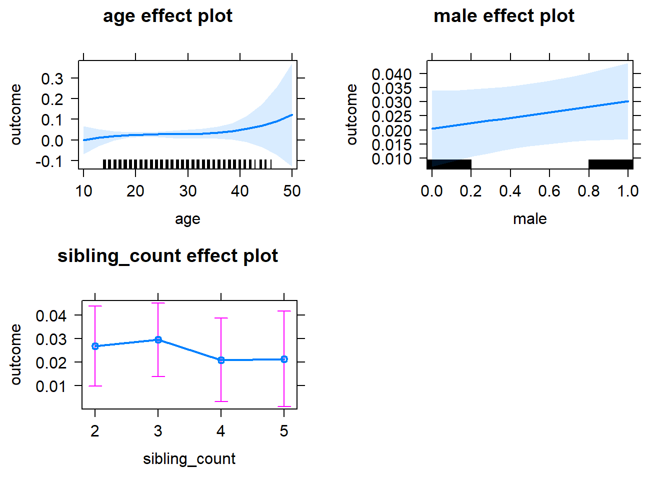
Add Birth Order Linear
Model Summary
tidy(m2_birthorder_linear, conf.int = T, conf.level = 0.995)| effect | group | term | estimate | std.error | statistic | df | p.value | conf.low | conf.high |
|---|---|---|---|---|---|---|---|---|---|
| fixed | NA | (Intercept) | -0.09434 | 0.1281 | -0.7367 | 3109 | 0.4614 | -0.4538 | 0.2651 |
| fixed | NA | birth_order | -0.0006958 | 0.00284 | -0.245 | 3109 | 0.8065 | -0.008668 | 0.007277 |
| fixed | NA | poly(age, 3, raw = TRUE)1 | 0.01348 | 0.01596 | 0.8446 | 3109 | 0.3984 | -0.03132 | 0.05829 |
| fixed | NA | poly(age, 3, raw = TRUE)2 | -0.0005127 | 0.0006323 | -0.8109 | 3109 | 0.4175 | -0.002288 | 0.001262 |
| fixed | NA | poly(age, 3, raw = TRUE)3 | 0.00000656 | 0.000007926 | 0.8277 | 3109 | 0.4079 | -0.00001569 | 0.00002881 |
| fixed | NA | male | 0.009681 | 0.00546 | 1.773 | 3109 | 0.07633 | -0.005646 | 0.02501 |
| fixed | NA | sibling_count3 | 0.003021 | 0.007286 | 0.4147 | 3109 | 0.6784 | -0.01743 | 0.02347 |
| fixed | NA | sibling_count4 | -0.005087 | 0.008286 | -0.614 | 3109 | 0.5393 | -0.02835 | 0.01817 |
| fixed | NA | sibling_count5 | -0.00425 | 0.009738 | -0.4364 | 3109 | 0.6626 | -0.03159 | 0.02309 |
| ran_pars | mother_pidlink | sd__(Intercept) | 0 | NA | NA | NA | NA | NA | NA |
| ran_pars | Residual | sd__Observation | 0.1522 | NA | NA | NA | NA | NA | NA |
Coefficient Plot
plot_birthorder2(m2_birthorder_linear, separate = FALSE)
Add Birth Order Factor
Model Summary
m3_birthorder_nonlinear = update(m1_covariates_only, formula = . ~ . + birth_order_nonlinear)## boundary (singular) fit: see ?isSingulartidy(m3_birthorder_nonlinear, conf.int = T, conf.level = 0.995)| effect | group | term | estimate | std.error | statistic | df | p.value | conf.low | conf.high |
|---|---|---|---|---|---|---|---|---|---|
| fixed | NA | (Intercept) | -0.09568 | 0.1281 | -0.7469 | 3106 | 0.4552 | -0.4553 | 0.2639 |
| fixed | NA | poly(age, 3, raw = TRUE)1 | 0.01336 | 0.01597 | 0.8364 | 3106 | 0.403 | -0.03147 | 0.05819 |
| fixed | NA | poly(age, 3, raw = TRUE)2 | -0.0005075 | 0.0006326 | -0.8021 | 3106 | 0.4225 | -0.002283 | 0.001268 |
| fixed | NA | poly(age, 3, raw = TRUE)3 | 0.000006494 | 0.00000793 | 0.819 | 3106 | 0.4129 | -0.00001577 | 0.00002875 |
| fixed | NA | male | 0.009854 | 0.005463 | 1.804 | 3106 | 0.0714 | -0.005483 | 0.02519 |
| fixed | NA | sibling_count3 | 0.003745 | 0.007435 | 0.5037 | 3106 | 0.6145 | -0.01713 | 0.02462 |
| fixed | NA | sibling_count4 | -0.003304 | 0.00844 | -0.3915 | 3106 | 0.6955 | -0.027 | 0.02039 |
| fixed | NA | sibling_count5 | -0.004296 | 0.009915 | -0.4333 | 3106 | 0.6648 | -0.03213 | 0.02354 |
| fixed | NA | birth_order_nonlinear2 | 0.003639 | 0.006613 | 0.5503 | 3106 | 0.5822 | -0.01492 | 0.0222 |
| fixed | NA | birth_order_nonlinear3 | -0.004395 | 0.008476 | -0.5185 | 3106 | 0.6041 | -0.02819 | 0.0194 |
| fixed | NA | birth_order_nonlinear4 | -0.006257 | 0.01122 | -0.5575 | 3106 | 0.5773 | -0.03776 | 0.02525 |
| fixed | NA | birth_order_nonlinear5 | 0.007926 | 0.01697 | 0.4672 | 3106 | 0.6404 | -0.0397 | 0.05555 |
| ran_pars | mother_pidlink | sd__(Intercept) | 0 | NA | NA | NA | NA | NA | NA |
| ran_pars | Residual | sd__Observation | 0.1523 | NA | NA | NA | NA | NA | NA |
Coefficient Plot
plot_birthorder(m3_birthorder_nonlinear, separate = FALSE)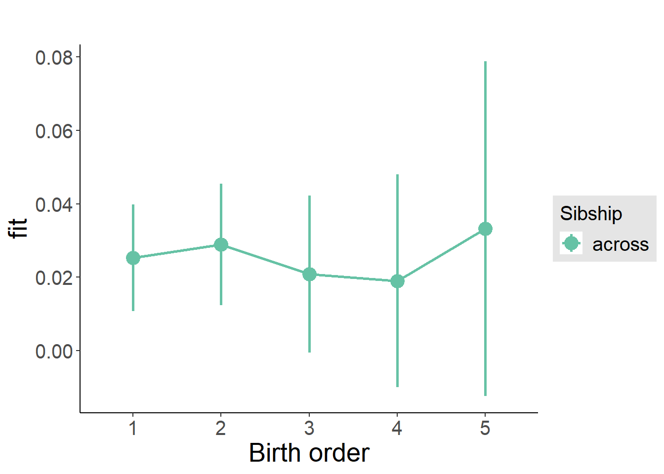
Add Interaction
Model Summary
m4_interaction = update(m3_birthorder_nonlinear, formula = . ~ . - birth_order_nonlinear - sibling_count + count_birth_order)## boundary (singular) fit: see ?isSingulartidy(m4_interaction, conf.int = T, conf.level = 0.995)| effect | group | term | estimate | std.error | statistic | df | p.value | conf.low | conf.high |
|---|---|---|---|---|---|---|---|---|---|
| fixed | NA | (Intercept) | -0.09762 | 0.1283 | -0.7609 | 3100 | 0.4468 | -0.4578 | 0.2625 |
| fixed | NA | poly(age, 3, raw = TRUE)1 | 0.01386 | 0.01599 | 0.867 | 3100 | 0.386 | -0.03102 | 0.05874 |
| fixed | NA | poly(age, 3, raw = TRUE)2 | -0.0005246 | 0.0006333 | -0.8283 | 3100 | 0.4076 | -0.002302 | 0.001253 |
| fixed | NA | poly(age, 3, raw = TRUE)3 | 0.000006657 | 0.000007938 | 0.8387 | 3100 | 0.4017 | -0.00001562 | 0.00002894 |
| fixed | NA | male | 0.01005 | 0.005472 | 1.838 | 3100 | 0.06623 | -0.005305 | 0.02541 |
| fixed | NA | count_birth_order2/2 | -0.004029 | 0.01122 | -0.359 | 3100 | 0.7196 | -0.03553 | 0.02747 |
| fixed | NA | count_birth_order1/3 | -0.003772 | 0.009773 | -0.386 | 3100 | 0.6995 | -0.0312 | 0.02366 |
| fixed | NA | count_birth_order2/3 | 0.007183 | 0.01061 | 0.6771 | 3100 | 0.4984 | -0.02259 | 0.03696 |
| fixed | NA | count_birth_order3/3 | 0.002688 | 0.01185 | 0.2267 | 3100 | 0.8207 | -0.03059 | 0.03596 |
| fixed | NA | count_birth_order1/4 | 0.0003133 | 0.01232 | 0.02542 | 3100 | 0.9797 | -0.03428 | 0.0349 |
| fixed | NA | count_birth_order2/4 | 0.001801 | 0.01243 | 0.1448 | 3100 | 0.8849 | -0.03309 | 0.0367 |
| fixed | NA | count_birth_order3/4 | -0.02074 | 0.01384 | -1.499 | 3100 | 0.1339 | -0.05958 | 0.0181 |
| fixed | NA | count_birth_order4/4 | -0.01514 | 0.01345 | -1.125 | 3100 | 0.2605 | -0.0529 | 0.02262 |
| fixed | NA | count_birth_order1/5 | -0.01139 | 0.0153 | -0.7442 | 3100 | 0.4568 | -0.05435 | 0.03157 |
| fixed | NA | count_birth_order2/5 | -0.005266 | 0.01738 | -0.3031 | 3100 | 0.7619 | -0.05404 | 0.04351 |
| fixed | NA | count_birth_order3/5 | -0.008987 | 0.01591 | -0.5649 | 3100 | 0.5722 | -0.05364 | 0.03567 |
| fixed | NA | count_birth_order4/5 | -0.00826 | 0.01629 | -0.5069 | 3100 | 0.6122 | -0.054 | 0.03748 |
| fixed | NA | count_birth_order5/5 | 0.001075 | 0.01594 | 0.06742 | 3100 | 0.9463 | -0.04366 | 0.04581 |
| ran_pars | mother_pidlink | sd__(Intercept) | 0 | NA | NA | NA | NA | NA | NA |
| ran_pars | Residual | sd__Observation | 0.1523 | NA | NA | NA | NA | NA | NA |
Coefficient Plot
plot_birthorder(m4_interaction)
Model Comparison
###### Model 1 - Model 2
anova(m1_covariates_only, m2_birthorder_linear, m3_birthorder_nonlinear, m4_interaction)## refitting model(s) with ML (instead of REML)| Df | AIC | BIC | logLik | deviance | Chisq | Chi Df | Pr(>Chisq) |
|---|---|---|---|---|---|---|---|
| 10 | -2879 | -2818 | 1449 | -2899 | NA | NA | NA |
| 11 | -2877 | -2810 | 1449 | -2899 | 0.06019 | 1 | 0.8062 |
| 14 | -2872 | -2788 | 1450 | -2900 | 1.531 | 3 | 0.6751 |
| 20 | -2863 | -2742 | 1452 | -2903 | 2.93 | 6 | 0.8175 |
Parental full sibling order
outcome_parental_m1 <- update(m2_birthorder_linear, data = birthorder %>%
mutate(sibling_count = sibling_count_genes_factor,
birth_order_nonlinear = birthorder_genes_factor,
birth_order = birthorder_genes,
count_birth_order = count_birthorder_genes
) %>%
filter(sibling_count != "1"))## boundary (singular) fit: see ?isSingularcompare_models_markdown(outcome_parental_m1)Basic Model
Model Summary
m1_covariates_only <- update(m2_birthorder_linear, formula = . ~ . - birth_order)## boundary (singular) fit: see ?isSingulartidy(m1_covariates_only, conf.int = T, conf.level = 0.995)| effect | group | term | estimate | std.error | statistic | df | p.value | conf.low | conf.high |
|---|---|---|---|---|---|---|---|---|---|
| fixed | NA | (Intercept) | -0.1276 | 0.1259 | -1.014 | 3284 | 0.3108 | -0.481 | 0.2258 |
| fixed | NA | poly(age, 3, raw = TRUE)1 | 0.01847 | 0.0157 | 1.177 | 3284 | 0.2394 | -0.02559 | 0.06254 |
| fixed | NA | poly(age, 3, raw = TRUE)2 | -0.0007421 | 0.0006219 | -1.193 | 3284 | 0.2328 | -0.002488 | 0.001004 |
| fixed | NA | poly(age, 3, raw = TRUE)3 | 0.000009978 | 0.000007806 | 1.278 | 3284 | 0.2013 | -0.00001193 | 0.00003189 |
| fixed | NA | male | 0.005732 | 0.005374 | 1.067 | 3284 | 0.2862 | -0.009352 | 0.02082 |
| fixed | NA | sibling_count3 | -0.001784 | 0.006659 | -0.2678 | 3284 | 0.7888 | -0.02048 | 0.01691 |
| fixed | NA | sibling_count4 | -0.007831 | 0.007468 | -1.049 | 3284 | 0.2945 | -0.02879 | 0.01313 |
| fixed | NA | sibling_count5 | 0.001724 | 0.009164 | 0.1882 | 3284 | 0.8508 | -0.024 | 0.02745 |
| ran_pars | mother_pidlink | sd__(Intercept) | 0 | NA | NA | NA | NA | NA | NA |
| ran_pars | Residual | sd__Observation | 0.1539 | NA | NA | NA | NA | NA | NA |
Coefficient Plot
plot(allEffects(m1_covariates_only, confidence.level = 0.995))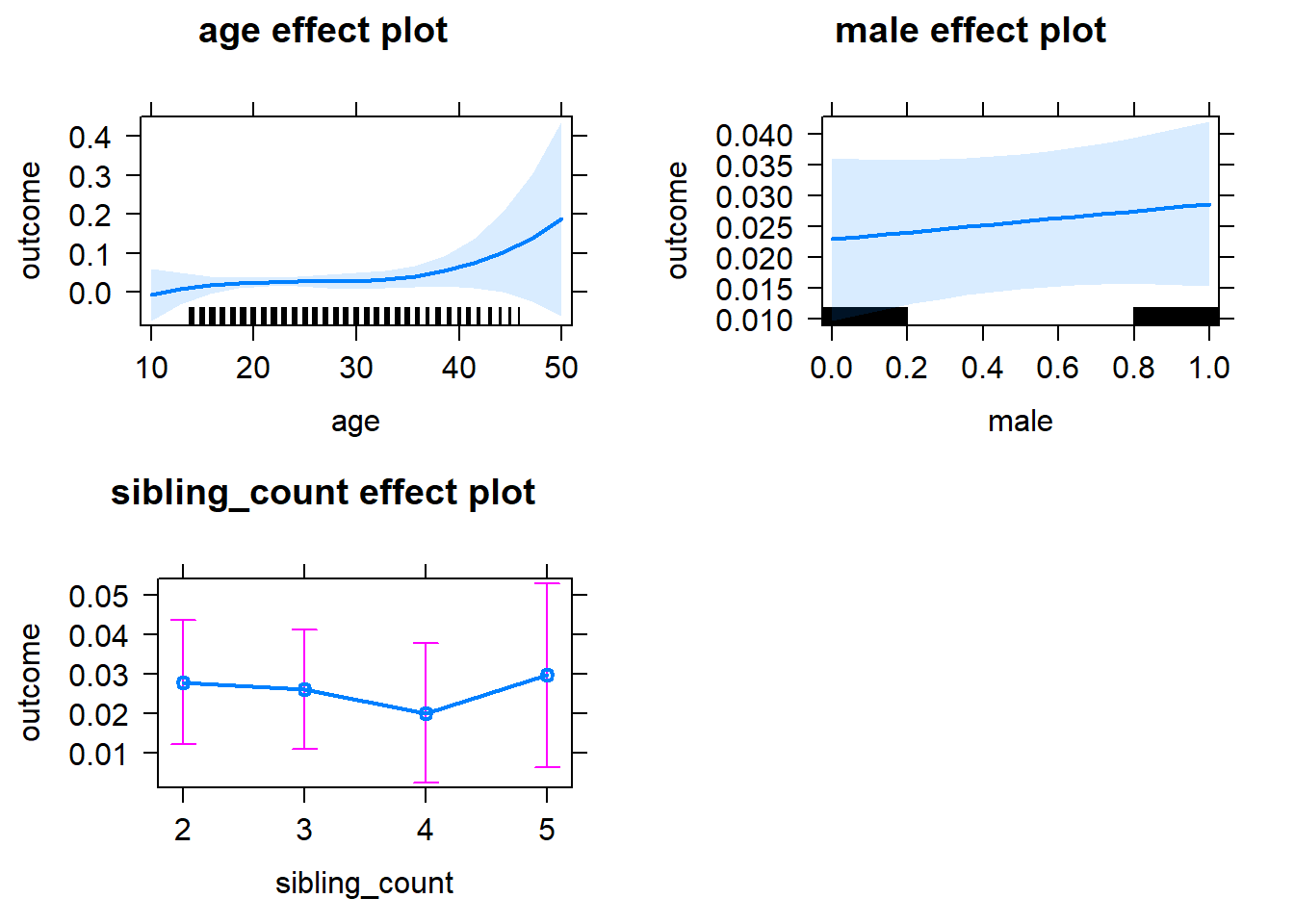
Add Birth Order Linear
Model Summary
tidy(m2_birthorder_linear, conf.int = T, conf.level = 0.995)| effect | group | term | estimate | std.error | statistic | df | p.value | conf.low | conf.high |
|---|---|---|---|---|---|---|---|---|---|
| fixed | NA | (Intercept) | -0.1264 | 0.126 | -1.003 | 3283 | 0.3161 | -0.4801 | 0.2274 |
| fixed | NA | birth_order | -0.000671 | 0.002963 | -0.2265 | 3283 | 0.8208 | -0.008987 | 0.007645 |
| fixed | NA | poly(age, 3, raw = TRUE)1 | 0.01843 | 0.0157 | 1.174 | 3283 | 0.2407 | -0.02565 | 0.0625 |
| fixed | NA | poly(age, 3, raw = TRUE)2 | -0.00074 | 0.0006221 | -1.19 | 3283 | 0.2343 | -0.002486 | 0.001006 |
| fixed | NA | poly(age, 3, raw = TRUE)3 | 0.000009946 | 0.000007808 | 1.274 | 3283 | 0.2028 | -0.00001197 | 0.00003186 |
| fixed | NA | male | 0.005745 | 0.005375 | 1.069 | 3283 | 0.2852 | -0.009342 | 0.02083 |
| fixed | NA | sibling_count3 | -0.001483 | 0.006791 | -0.2184 | 3283 | 0.8271 | -0.02054 | 0.01758 |
| fixed | NA | sibling_count4 | -0.007111 | 0.008118 | -0.8759 | 3283 | 0.3812 | -0.0299 | 0.01568 |
| fixed | NA | sibling_count5 | 0.002881 | 0.01049 | 0.2746 | 3283 | 0.7837 | -0.02657 | 0.03233 |
| ran_pars | mother_pidlink | sd__(Intercept) | 0 | NA | NA | NA | NA | NA | NA |
| ran_pars | Residual | sd__Observation | 0.154 | NA | NA | NA | NA | NA | NA |
Coefficient Plot
plot_birthorder2(m2_birthorder_linear, separate = FALSE)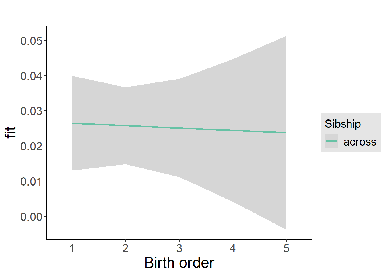
Add Birth Order Factor
Model Summary
m3_birthorder_nonlinear = update(m1_covariates_only, formula = . ~ . + birth_order_nonlinear)## boundary (singular) fit: see ?isSingulartidy(m3_birthorder_nonlinear, conf.int = T, conf.level = 0.995)| effect | group | term | estimate | std.error | statistic | df | p.value | conf.low | conf.high |
|---|---|---|---|---|---|---|---|---|---|
| fixed | NA | (Intercept) | -0.135 | 0.1261 | -1.07 | 3280 | 0.2845 | -0.489 | 0.219 |
| fixed | NA | poly(age, 3, raw = TRUE)1 | 0.01917 | 0.01572 | 1.22 | 3280 | 0.2226 | -0.02495 | 0.06329 |
| fixed | NA | poly(age, 3, raw = TRUE)2 | -0.0007671 | 0.0006227 | -1.232 | 3280 | 0.2181 | -0.002515 | 0.0009807 |
| fixed | NA | poly(age, 3, raw = TRUE)3 | 0.00001024 | 0.000007815 | 1.31 | 3280 | 0.1903 | -0.0000117 | 0.00003217 |
| fixed | NA | male | 0.005733 | 0.005377 | 1.066 | 3280 | 0.2864 | -0.00936 | 0.02083 |
| fixed | NA | sibling_count3 | -0.002652 | 0.006939 | -0.3822 | 3280 | 0.7024 | -0.02213 | 0.01683 |
| fixed | NA | sibling_count4 | -0.007732 | 0.008295 | -0.9321 | 3280 | 0.3513 | -0.03102 | 0.01555 |
| fixed | NA | sibling_count5 | 0.00662 | 0.01085 | 0.6103 | 3280 | 0.5417 | -0.02383 | 0.03706 |
| fixed | NA | birth_order_nonlinear2 | 0.004309 | 0.006425 | 0.6707 | 3280 | 0.5025 | -0.01373 | 0.02234 |
| fixed | NA | birth_order_nonlinear3 | 0.004283 | 0.008403 | 0.5098 | 3280 | 0.6103 | -0.0193 | 0.02787 |
| fixed | NA | birth_order_nonlinear4 | -0.003198 | 0.01173 | -0.2727 | 3280 | 0.7851 | -0.03612 | 0.02972 |
| fixed | NA | birth_order_nonlinear5 | -0.01996 | 0.01966 | -1.016 | 3280 | 0.3099 | -0.07514 | 0.03522 |
| ran_pars | mother_pidlink | sd__(Intercept) | 0 | NA | NA | NA | NA | NA | NA |
| ran_pars | Residual | sd__Observation | 0.154 | NA | NA | NA | NA | NA | NA |
Coefficient Plot
plot_birthorder(m3_birthorder_nonlinear, separate = FALSE)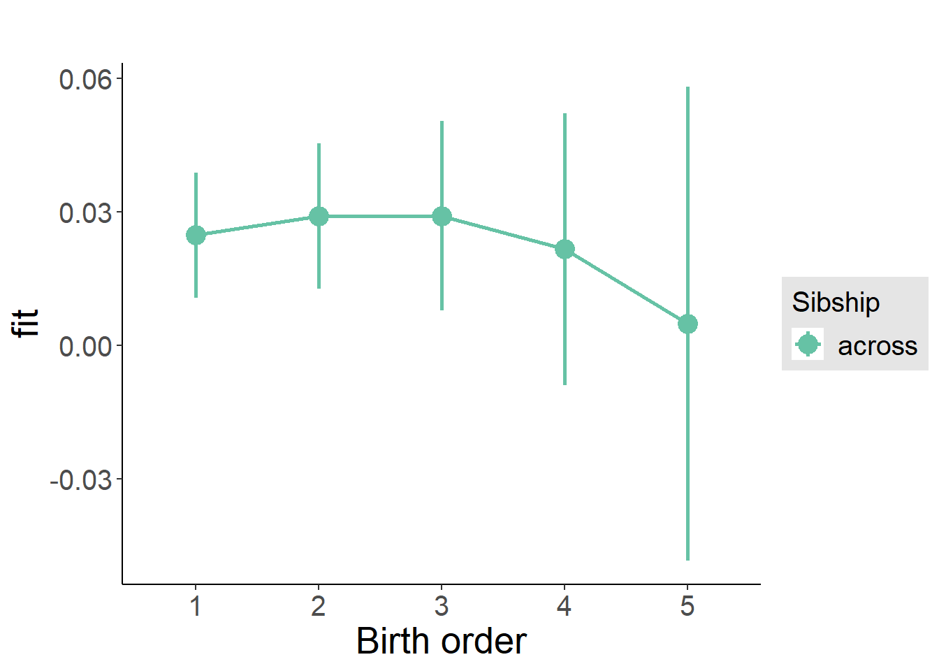
Add Interaction
Model Summary
m4_interaction = update(m3_birthorder_nonlinear, formula = . ~ . - birth_order_nonlinear - sibling_count + count_birth_order)## boundary (singular) fit: see ?isSingulartidy(m4_interaction, conf.int = T, conf.level = 0.995)| effect | group | term | estimate | std.error | statistic | df | p.value | conf.low | conf.high |
|---|---|---|---|---|---|---|---|---|---|
| fixed | NA | (Intercept) | -0.1376 | 0.1262 | -1.09 | 3274 | 0.2758 | -0.492 | 0.2168 |
| fixed | NA | poly(age, 3, raw = TRUE)1 | 0.01976 | 0.01573 | 1.257 | 3274 | 0.209 | -0.02439 | 0.06391 |
| fixed | NA | poly(age, 3, raw = TRUE)2 | -0.0007861 | 0.0006231 | -1.262 | 3274 | 0.2072 | -0.002535 | 0.000963 |
| fixed | NA | poly(age, 3, raw = TRUE)3 | 0.00001043 | 0.00000782 | 1.333 | 3274 | 0.1826 | -0.00001153 | 0.00003238 |
| fixed | NA | male | 0.005953 | 0.005382 | 1.106 | 3274 | 0.2687 | -0.009154 | 0.02106 |
| fixed | NA | count_birth_order2/2 | -0.004536 | 0.01013 | -0.4477 | 3274 | 0.6544 | -0.03298 | 0.02391 |
| fixed | NA | count_birth_order1/3 | -0.01268 | 0.009092 | -1.395 | 3274 | 0.1632 | -0.0382 | 0.01284 |
| fixed | NA | count_birth_order2/3 | 0.003404 | 0.01012 | 0.3362 | 3274 | 0.7368 | -0.02502 | 0.03182 |
| fixed | NA | count_birth_order3/3 | 0.005291 | 0.01113 | 0.4752 | 3274 | 0.6347 | -0.02597 | 0.03655 |
| fixed | NA | count_birth_order1/4 | -0.004382 | 0.01232 | -0.3557 | 3274 | 0.7221 | -0.03896 | 0.0302 |
| fixed | NA | count_birth_order2/4 | -0.001983 | 0.01271 | -0.156 | 3274 | 0.876 | -0.03766 | 0.03369 |
| fixed | NA | count_birth_order3/4 | -0.01713 | 0.01307 | -1.311 | 3274 | 0.1899 | -0.05382 | 0.01955 |
| fixed | NA | count_birth_order4/4 | -0.01591 | 0.01334 | -1.193 | 3274 | 0.2331 | -0.05336 | 0.02154 |
| fixed | NA | count_birth_order1/5 | 0.005286 | 0.01779 | 0.2971 | 3274 | 0.7664 | -0.04465 | 0.05522 |
| fixed | NA | count_birth_order2/5 | -0.0002005 | 0.02026 | -0.009896 | 3274 | 0.9921 | -0.05706 | 0.05666 |
| fixed | NA | count_birth_order3/5 | 0.008486 | 0.01849 | 0.459 | 3274 | 0.6463 | -0.04341 | 0.06038 |
| fixed | NA | count_birth_order4/5 | 0.003727 | 0.01728 | 0.2156 | 3274 | 0.8293 | -0.04479 | 0.05225 |
| fixed | NA | count_birth_order5/5 | -0.01646 | 0.01795 | -0.917 | 3274 | 0.3592 | -0.06683 | 0.03392 |
| ran_pars | mother_pidlink | sd__(Intercept) | 0 | NA | NA | NA | NA | NA | NA |
| ran_pars | Residual | sd__Observation | 0.154 | NA | NA | NA | NA | NA | NA |
Coefficient Plot
plot_birthorder(m4_interaction)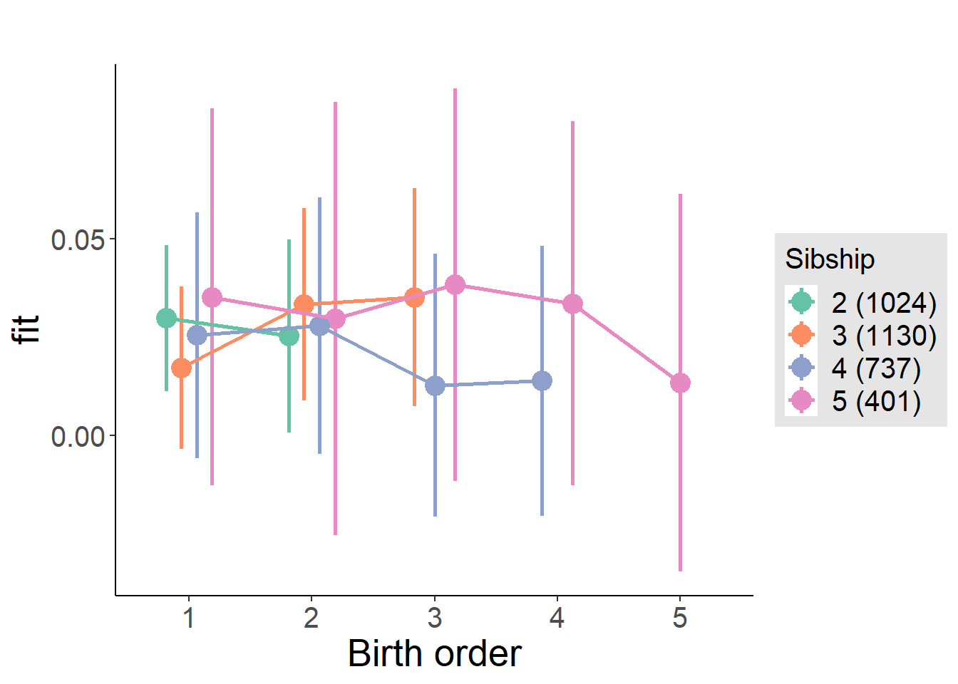
Model Comparison
###### Model 1 - Model 2
anova(m1_covariates_only, m2_birthorder_linear, m3_birthorder_nonlinear, m4_interaction)## refitting model(s) with ML (instead of REML)| Df | AIC | BIC | logLik | deviance | Chisq | Chi Df | Pr(>Chisq) |
|---|---|---|---|---|---|---|---|
| 10 | -2966 | -2905 | 1493 | -2986 | NA | NA | NA |
| 11 | -2964 | -2897 | 1493 | -2986 | 0.05144 | 1 | 0.8206 |
| 14 | -2960 | -2874 | 1494 | -2988 | 1.997 | 3 | 0.573 |
| 20 | -2952 | -2830 | 1496 | -2992 | 4.281 | 6 | 0.6387 |
Compare birth order specifications
library(coefplot)
multiplot(outcome_naive_m1, outcome_preg_m1, outcome_uterus_m1, outcome_parental_m1, dodgeHeight = 0.6,
intercept = FALSE)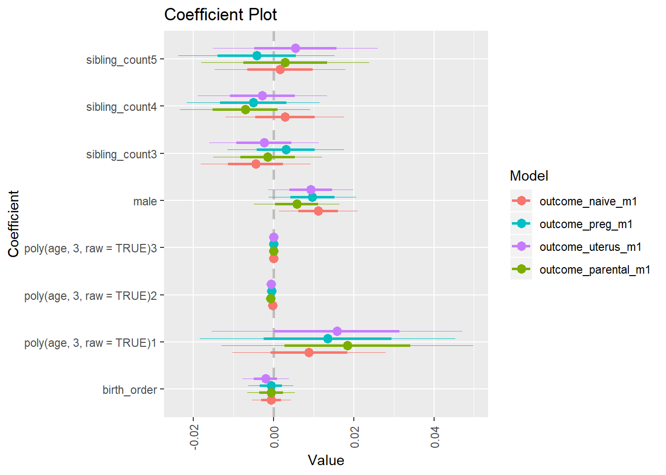
Elementary worked
birthorder <- birthorder %>% mutate(outcome = Elementary_worked)
model = lmer(outcome ~ birth_order + poly(age, 3, raw = TRUE) + male + sibling_count + (1 | mother_pidlink),
data = birthorder)
compare_birthorder_specs(model)Naive birth order
outcome_naive_m1 <- update(m2_birthorder_linear, data = birthorder %>%
mutate(sibling_count = sibling_count_naive_factor,
birth_order_nonlinear = birthorder_naive_factor,
birth_order = birthorder_naive,
count_birth_order = count_birthorder_naive) %>%
filter(sibling_count != "1"))
compare_models_markdown(outcome_naive_m1)Basic Model
Model Summary
m1_covariates_only <- update(m2_birthorder_linear, formula = . ~ . - birth_order)
tidy(m1_covariates_only, conf.int = T, conf.level = 0.995)| effect | group | term | estimate | std.error | statistic | df | p.value | conf.low | conf.high |
|---|---|---|---|---|---|---|---|---|---|
| fixed | NA | (Intercept) | -0.03812 | 0.09707 | -0.3927 | 4266 | 0.6946 | -0.3106 | 0.2344 |
| fixed | NA | poly(age, 3, raw = TRUE)1 | 0.006604 | 0.01127 | 0.5861 | 4275 | 0.5578 | -0.02503 | 0.03823 |
| fixed | NA | poly(age, 3, raw = TRUE)2 | -0.0002517 | 0.0004101 | -0.6138 | 4281 | 0.5394 | -0.001403 | 0.0008995 |
| fixed | NA | poly(age, 3, raw = TRUE)3 | 0.000003713 | 0.000004677 | 0.7938 | 4283 | 0.4274 | -0.000009416 | 0.00001684 |
| fixed | NA | male | 0.02374 | 0.005877 | 4.041 | 4210 | 0.00005428 | 0.007249 | 0.04024 |
| fixed | NA | sibling_count3 | -0.008451 | 0.00834 | -1.013 | 3393 | 0.311 | -0.03186 | 0.01496 |
| fixed | NA | sibling_count4 | 0.004285 | 0.008617 | 0.4972 | 3179 | 0.6191 | -0.0199 | 0.02847 |
| fixed | NA | sibling_count5 | 0.01206 | 0.008972 | 1.344 | 2833 | 0.1791 | -0.01313 | 0.03724 |
| ran_pars | mother_pidlink | sd__(Intercept) | 0.06971 | NA | NA | NA | NA | NA | NA |
| ran_pars | Residual | sd__Observation | 0.1806 | NA | NA | NA | NA | NA | NA |
Coefficient Plot
plot(allEffects(m1_covariates_only, confidence.level = 0.995))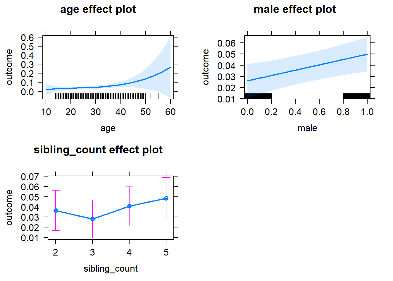
Add Birth Order Linear
Model Summary
tidy(m2_birthorder_linear, conf.int = T, conf.level = 0.995)| effect | group | term | estimate | std.error | statistic | df | p.value | conf.low | conf.high |
|---|---|---|---|---|---|---|---|---|---|
| fixed | NA | (Intercept) | -0.03277 | 0.09746 | -0.3363 | 4280 | 0.7367 | -0.3064 | 0.2408 |
| fixed | NA | birth_order | -0.001798 | 0.002928 | -0.6142 | 4026 | 0.5391 | -0.01002 | 0.00642 |
| fixed | NA | poly(age, 3, raw = TRUE)1 | 0.00624 | 0.01128 | 0.553 | 4280 | 0.5803 | -0.02544 | 0.03792 |
| fixed | NA | poly(age, 3, raw = TRUE)2 | -0.0002378 | 0.0004108 | -0.5789 | 4284 | 0.5627 | -0.001391 | 0.0009152 |
| fixed | NA | poly(age, 3, raw = TRUE)3 | 0.000003548 | 0.000004685 | 0.7574 | 4285 | 0.4489 | -0.000009603 | 0.0000167 |
| fixed | NA | male | 0.02377 | 0.005877 | 4.045 | 4209 | 0.00005335 | 0.007274 | 0.04027 |
| fixed | NA | sibling_count3 | -0.007728 | 0.008423 | -0.9174 | 3443 | 0.359 | -0.03137 | 0.01592 |
| fixed | NA | sibling_count4 | 0.006035 | 0.009077 | 0.6649 | 3392 | 0.5062 | -0.01944 | 0.03151 |
| fixed | NA | sibling_count5 | 0.01488 | 0.01008 | 1.476 | 3264 | 0.14 | -0.01342 | 0.04318 |
| ran_pars | mother_pidlink | sd__(Intercept) | 0.06967 | NA | NA | NA | NA | NA | NA |
| ran_pars | Residual | sd__Observation | 0.1806 | NA | NA | NA | NA | NA | NA |
Coefficient Plot
plot_birthorder2(m2_birthorder_linear, separate = FALSE)
Add Birth Order Factor
Model Summary
m3_birthorder_nonlinear = update(m1_covariates_only, formula = . ~ . + birth_order_nonlinear)
tidy(m3_birthorder_nonlinear, conf.int = T, conf.level = 0.995)| effect | group | term | estimate | std.error | statistic | df | p.value | conf.low | conf.high |
|---|---|---|---|---|---|---|---|---|---|
| fixed | NA | (Intercept) | -0.03893 | 0.0975 | -0.3993 | 4279 | 0.6897 | -0.3126 | 0.2348 |
| fixed | NA | poly(age, 3, raw = TRUE)1 | 0.006531 | 0.0113 | 0.578 | 4281 | 0.5633 | -0.02518 | 0.03825 |
| fixed | NA | poly(age, 3, raw = TRUE)2 | -0.0002489 | 0.0004112 | -0.6052 | 4283 | 0.5451 | -0.001403 | 0.0009054 |
| fixed | NA | poly(age, 3, raw = TRUE)3 | 0.000003673 | 0.000004689 | 0.7833 | 4284 | 0.4335 | -0.00000949 | 0.00001684 |
| fixed | NA | male | 0.02393 | 0.005877 | 4.072 | 4207 | 0.00004741 | 0.007436 | 0.04043 |
| fixed | NA | sibling_count3 | -0.005085 | 0.008542 | -0.5953 | 3529 | 0.5517 | -0.02906 | 0.01889 |
| fixed | NA | sibling_count4 | 0.008949 | 0.009241 | 0.9684 | 3495 | 0.3329 | -0.01699 | 0.03489 |
| fixed | NA | sibling_count5 | 0.01533 | 0.01018 | 1.506 | 3291 | 0.1321 | -0.01324 | 0.04391 |
| fixed | NA | birth_order_nonlinear2 | 0.003991 | 0.007057 | 0.5655 | 3576 | 0.5717 | -0.01582 | 0.0238 |
| fixed | NA | birth_order_nonlinear3 | -0.01552 | 0.009022 | -1.72 | 3746 | 0.08549 | -0.04084 | 0.009806 |
| fixed | NA | birth_order_nonlinear4 | -0.005023 | 0.01171 | -0.4291 | 3881 | 0.6679 | -0.03789 | 0.02784 |
| fixed | NA | birth_order_nonlinear5 | 0.006543 | 0.0163 | 0.4014 | 3958 | 0.6882 | -0.03922 | 0.0523 |
| ran_pars | mother_pidlink | sd__(Intercept) | 0.06925 | NA | NA | NA | NA | NA | NA |
| ran_pars | Residual | sd__Observation | 0.1807 | NA | NA | NA | NA | NA | NA |
Coefficient Plot
plot_birthorder(m3_birthorder_nonlinear, separate = FALSE)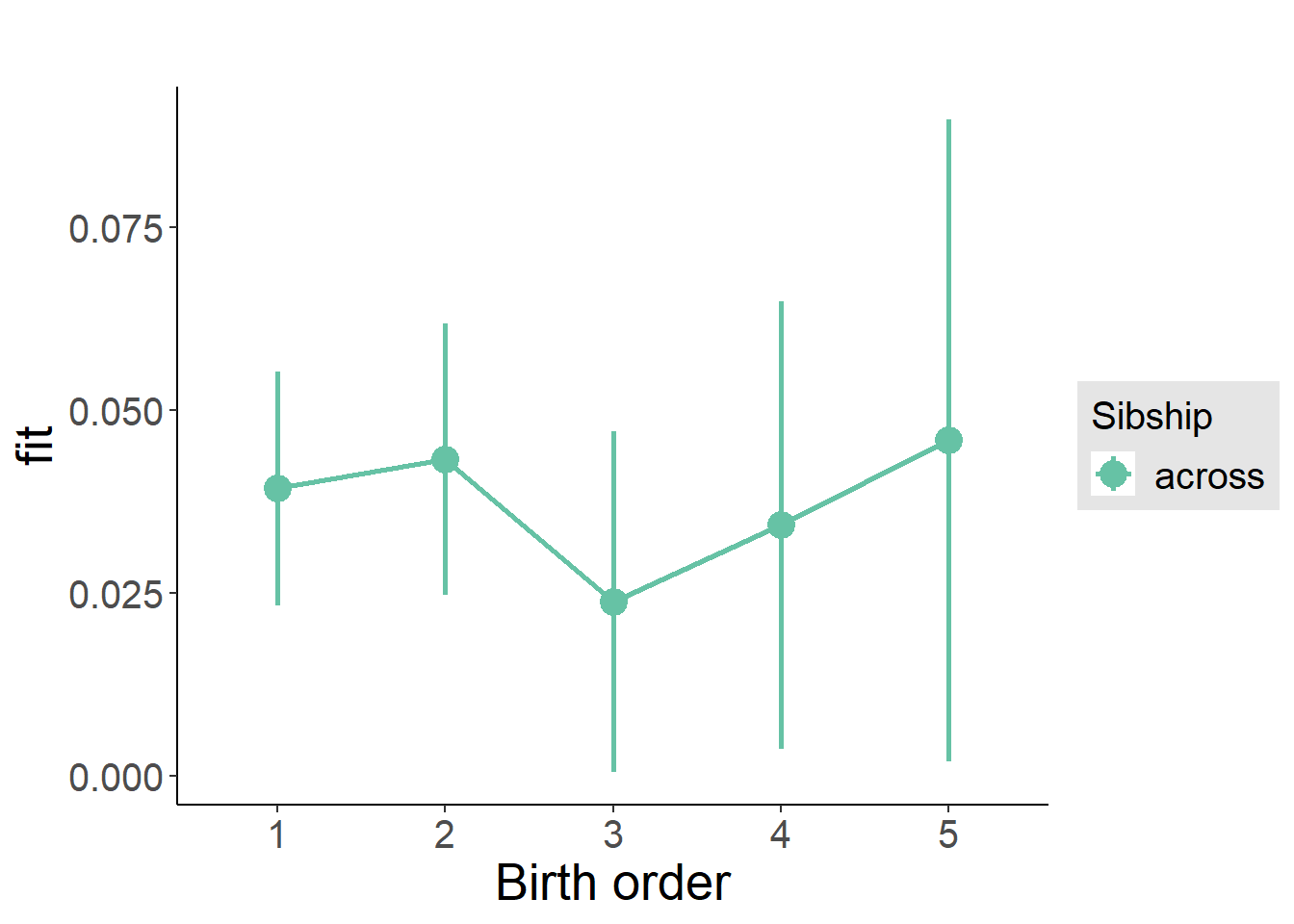
Add Interaction
Model Summary
m4_interaction = update(m3_birthorder_nonlinear, formula = . ~ . - birth_order_nonlinear - sibling_count + count_birth_order)
tidy(m4_interaction, conf.int = T, conf.level = 0.995)| effect | group | term | estimate | std.error | statistic | df | p.value | conf.low | conf.high |
|---|---|---|---|---|---|---|---|---|---|
| fixed | NA | (Intercept) | -0.0389 | 0.09764 | -0.3984 | 4273 | 0.6904 | -0.313 | 0.2352 |
| fixed | NA | poly(age, 3, raw = TRUE)1 | 0.006551 | 0.01131 | 0.5794 | 4275 | 0.5624 | -0.02519 | 0.03829 |
| fixed | NA | poly(age, 3, raw = TRUE)2 | -0.0002507 | 0.0004116 | -0.6091 | 4277 | 0.5425 | -0.001406 | 0.0009046 |
| fixed | NA | poly(age, 3, raw = TRUE)3 | 0.000003709 | 0.000004694 | 0.7902 | 4278 | 0.4294 | -0.000009467 | 0.00001688 |
| fixed | NA | male | 0.02387 | 0.005882 | 4.058 | 4199 | 0.0000505 | 0.007355 | 0.04038 |
| fixed | NA | count_birth_order2/2 | 0.003992 | 0.01233 | 0.3238 | 3700 | 0.7461 | -0.03062 | 0.0386 |
| fixed | NA | count_birth_order1/3 | -0.004001 | 0.01101 | -0.3633 | 4276 | 0.7164 | -0.03491 | 0.02691 |
| fixed | NA | count_birth_order2/3 | 0.0007906 | 0.01224 | 0.06459 | 4278 | 0.9485 | -0.03357 | 0.03515 |
| fixed | NA | count_birth_order3/3 | -0.02583 | 0.0141 | -1.833 | 4271 | 0.06694 | -0.0654 | 0.01374 |
| fixed | NA | count_birth_order1/4 | 0.001996 | 0.01299 | 0.1536 | 4278 | 0.8779 | -0.03447 | 0.03846 |
| fixed | NA | count_birth_order2/4 | 0.01665 | 0.01346 | 1.237 | 4273 | 0.2162 | -0.02113 | 0.05442 |
| fixed | NA | count_birth_order3/4 | 0.002168 | 0.01453 | 0.1492 | 4260 | 0.8814 | -0.03863 | 0.04297 |
| fixed | NA | count_birth_order4/4 | 0.0001625 | 0.01507 | 0.01079 | 4267 | 0.9914 | -0.04213 | 0.04246 |
| fixed | NA | count_birth_order1/5 | 0.02296 | 0.01499 | 1.532 | 4271 | 0.1256 | -0.0191 | 0.06503 |
| fixed | NA | count_birth_order2/5 | 0.009444 | 0.016 | 0.5902 | 4240 | 0.5551 | -0.03547 | 0.05436 |
| fixed | NA | count_birth_order3/5 | -0.003822 | 0.01573 | -0.243 | 4231 | 0.808 | -0.04797 | 0.04033 |
| fixed | NA | count_birth_order4/5 | 0.01533 | 0.01663 | 0.9216 | 4226 | 0.3568 | -0.03136 | 0.06202 |
| fixed | NA | count_birth_order5/5 | 0.02184 | 0.01592 | 1.372 | 4249 | 0.17 | -0.02283 | 0.06652 |
| ran_pars | mother_pidlink | sd__(Intercept) | 0.06957 | NA | NA | NA | NA | NA | NA |
| ran_pars | Residual | sd__Observation | 0.1807 | NA | NA | NA | NA | NA | NA |
Coefficient Plot
plot_birthorder(m4_interaction)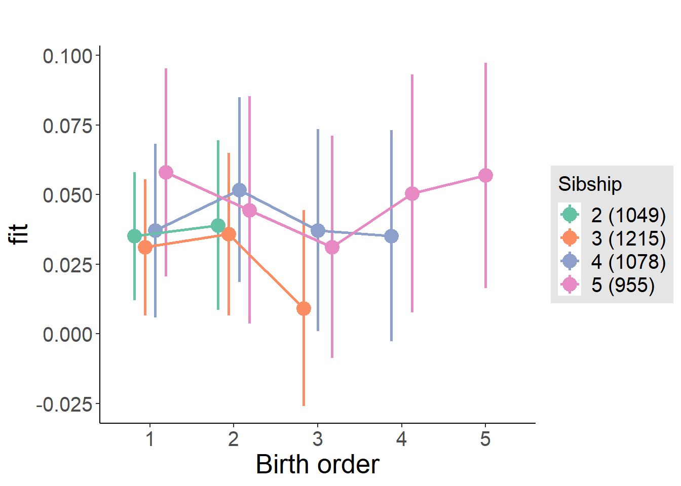
Model Comparison
###### Model 1 - Model 2
anova(m1_covariates_only, m2_birthorder_linear, m3_birthorder_nonlinear, m4_interaction)## refitting model(s) with ML (instead of REML)| Df | AIC | BIC | logLik | deviance | Chisq | Chi Df | Pr(>Chisq) |
|---|---|---|---|---|---|---|---|
| 10 | -1925 | -1861 | 972.5 | -1945 | NA | NA | NA |
| 11 | -1923 | -1853 | 972.7 | -1945 | 0.3781 | 1 | 0.5386 |
| 14 | -1922 | -1833 | 975 | -1950 | 4.648 | 3 | 0.1994 |
| 20 | -1912 | -1785 | 976.2 | -1952 | 2.449 | 6 | 0.8742 |
Maternal birth order
outcome_uterus_m1 <- update(m2_birthorder_linear, data = birthorder %>%
mutate(sibling_count = sibling_count_uterus_alive_factor,
birth_order_nonlinear = birthorder_uterus_alive_factor,
birth_order = birthorder_uterus_alive,
count_birth_order = count_birthorder_uterus_alive) %>%
filter(sibling_count != "1"))
compare_models_markdown(outcome_uterus_m1)Basic Model
Model Summary
m1_covariates_only <- update(m2_birthorder_linear, formula = . ~ . - birth_order)
tidy(m1_covariates_only, conf.int = T, conf.level = 0.995)| effect | group | term | estimate | std.error | statistic | df | p.value | conf.low | conf.high |
|---|---|---|---|---|---|---|---|---|---|
| fixed | NA | (Intercept) | 0.1676 | 0.14 | 1.197 | 3302 | 0.2314 | -0.2254 | 0.5605 |
| fixed | NA | poly(age, 3, raw = TRUE)1 | -0.02047 | 0.01748 | -1.171 | 3308 | 0.2417 | -0.06954 | 0.0286 |
| fixed | NA | poly(age, 3, raw = TRUE)2 | 0.0008317 | 0.0006936 | 1.199 | 3311 | 0.2306 | -0.001115 | 0.002779 |
| fixed | NA | poly(age, 3, raw = TRUE)3 | -0.00001056 | 0.000008717 | -1.211 | 3308 | 0.2259 | -0.00003503 | 0.00001391 |
| fixed | NA | male | 0.02121 | 0.005949 | 3.566 | 3292 | 0.0003681 | 0.004513 | 0.03791 |
| fixed | NA | sibling_count3 | 0.002832 | 0.007646 | 0.3704 | 2729 | 0.7111 | -0.01863 | 0.0243 |
| fixed | NA | sibling_count4 | 0.02947 | 0.008584 | 3.433 | 2525 | 0.0006058 | 0.005376 | 0.05357 |
| fixed | NA | sibling_count5 | 0.02129 | 0.0102 | 2.087 | 2443 | 0.03699 | -0.007345 | 0.04992 |
| ran_pars | mother_pidlink | sd__(Intercept) | 0.05795 | NA | NA | NA | NA | NA | NA |
| ran_pars | Residual | sd__Observation | 0.1618 | NA | NA | NA | NA | NA | NA |
Coefficient Plot
plot(allEffects(m1_covariates_only, confidence.level = 0.995))
Add Birth Order Linear
Model Summary
tidy(m2_birthorder_linear, conf.int = T, conf.level = 0.995)| effect | group | term | estimate | std.error | statistic | df | p.value | conf.low | conf.high |
|---|---|---|---|---|---|---|---|---|---|
| fixed | NA | (Intercept) | 0.166 | 0.1402 | 1.184 | 3303 | 0.2364 | -0.2275 | 0.5595 |
| fixed | NA | birth_order | 0.0007245 | 0.003239 | 0.2237 | 3274 | 0.823 | -0.008367 | 0.009816 |
| fixed | NA | poly(age, 3, raw = TRUE)1 | -0.0204 | 0.01749 | -1.166 | 3308 | 0.2435 | -0.06948 | 0.02869 |
| fixed | NA | poly(age, 3, raw = TRUE)2 | 0.0008289 | 0.0006938 | 1.195 | 3310 | 0.2323 | -0.001119 | 0.002776 |
| fixed | NA | poly(age, 3, raw = TRUE)3 | -0.00001052 | 0.00000872 | -1.207 | 3307 | 0.2277 | -0.000035 | 0.00001396 |
| fixed | NA | male | 0.02119 | 0.00595 | 3.562 | 3291 | 0.0003733 | 0.004492 | 0.0379 |
| fixed | NA | sibling_count3 | 0.002495 | 0.007793 | 0.3202 | 2759 | 0.7488 | -0.01938 | 0.02437 |
| fixed | NA | sibling_count4 | 0.02868 | 0.009288 | 3.088 | 2634 | 0.002038 | 0.002607 | 0.05475 |
| fixed | NA | sibling_count5 | 0.01998 | 0.01177 | 1.697 | 2690 | 0.08974 | -0.01306 | 0.05301 |
| ran_pars | mother_pidlink | sd__(Intercept) | 0.05791 | NA | NA | NA | NA | NA | NA |
| ran_pars | Residual | sd__Observation | 0.1618 | NA | NA | NA | NA | NA | NA |
Coefficient Plot
plot_birthorder2(m2_birthorder_linear, separate = FALSE)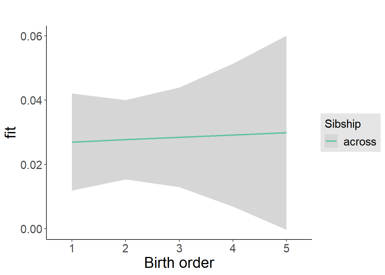
Add Birth Order Factor
Model Summary
m3_birthorder_nonlinear = update(m1_covariates_only, formula = . ~ . + birth_order_nonlinear)
tidy(m3_birthorder_nonlinear, conf.int = T, conf.level = 0.995)| effect | group | term | estimate | std.error | statistic | df | p.value | conf.low | conf.high |
|---|---|---|---|---|---|---|---|---|---|
| fixed | NA | (Intercept) | 0.169 | 0.1403 | 1.204 | 3302 | 0.2285 | -0.2249 | 0.5628 |
| fixed | NA | poly(age, 3, raw = TRUE)1 | -0.02081 | 0.01751 | -1.189 | 3306 | 0.2346 | -0.06995 | 0.02833 |
| fixed | NA | poly(age, 3, raw = TRUE)2 | 0.0008468 | 0.0006945 | 1.219 | 3307 | 0.2229 | -0.001103 | 0.002796 |
| fixed | NA | poly(age, 3, raw = TRUE)3 | -0.00001075 | 0.000008727 | -1.232 | 3303 | 0.218 | -0.00003525 | 0.00001374 |
| fixed | NA | male | 0.02141 | 0.005953 | 3.597 | 3289 | 0.000327 | 0.004701 | 0.03812 |
| fixed | NA | sibling_count3 | 0.002689 | 0.007943 | 0.3385 | 2820 | 0.735 | -0.01961 | 0.02498 |
| fixed | NA | sibling_count4 | 0.03121 | 0.009465 | 3.298 | 2675 | 0.0009875 | 0.004645 | 0.05778 |
| fixed | NA | sibling_count5 | 0.01828 | 0.01209 | 1.512 | 2692 | 0.1308 | -0.01566 | 0.05222 |
| fixed | NA | birth_order_nonlinear2 | 0.002557 | 0.007035 | 0.3635 | 2788 | 0.7163 | -0.01719 | 0.0223 |
| fixed | NA | birth_order_nonlinear3 | 0.0005794 | 0.009267 | 0.06252 | 3130 | 0.9502 | -0.02543 | 0.02659 |
| fixed | NA | birth_order_nonlinear4 | -0.007226 | 0.01264 | -0.5717 | 3213 | 0.5676 | -0.04271 | 0.02826 |
| fixed | NA | birth_order_nonlinear5 | 0.02259 | 0.02049 | 1.103 | 3245 | 0.2702 | -0.03492 | 0.0801 |
| ran_pars | mother_pidlink | sd__(Intercept) | 0.05747 | NA | NA | NA | NA | NA | NA |
| ran_pars | Residual | sd__Observation | 0.162 | NA | NA | NA | NA | NA | NA |
Coefficient Plot
plot_birthorder(m3_birthorder_nonlinear, separate = FALSE)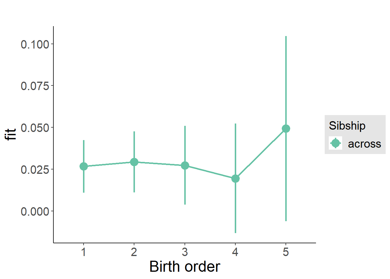
Add Interaction
Model Summary
m4_interaction = update(m3_birthorder_nonlinear, formula = . ~ . - birth_order_nonlinear - sibling_count + count_birth_order)
tidy(m4_interaction, conf.int = T, conf.level = 0.995)| effect | group | term | estimate | std.error | statistic | df | p.value | conf.low | conf.high |
|---|---|---|---|---|---|---|---|---|---|
| fixed | NA | (Intercept) | 0.17 | 0.1405 | 1.21 | 3296 | 0.2263 | -0.2244 | 0.5644 |
| fixed | NA | poly(age, 3, raw = TRUE)1 | -0.02099 | 0.01753 | -1.197 | 3300 | 0.2313 | -0.07019 | 0.02821 |
| fixed | NA | poly(age, 3, raw = TRUE)2 | 0.0008526 | 0.0006954 | 1.226 | 3301 | 0.2202 | -0.001099 | 0.002805 |
| fixed | NA | poly(age, 3, raw = TRUE)3 | -0.00001082 | 0.000008738 | -1.238 | 3297 | 0.2157 | -0.00003535 | 0.00001371 |
| fixed | NA | male | 0.02143 | 0.00596 | 3.596 | 3283 | 0.0003278 | 0.004703 | 0.03816 |
| fixed | NA | count_birth_order2/2 | 0.004241 | 0.01142 | 0.3715 | 2935 | 0.7103 | -0.02781 | 0.03629 |
| fixed | NA | count_birth_order1/3 | 0.003192 | 0.0102 | 0.3129 | 3300 | 0.7544 | -0.02545 | 0.03183 |
| fixed | NA | count_birth_order2/3 | 0.006016 | 0.01116 | 0.5392 | 3300 | 0.5898 | -0.0253 | 0.03734 |
| fixed | NA | count_birth_order3/3 | 0.003634 | 0.01248 | 0.2911 | 3298 | 0.771 | -0.0314 | 0.03867 |
| fixed | NA | count_birth_order1/4 | 0.039 | 0.01359 | 2.871 | 3300 | 0.00412 | 0.0008667 | 0.07714 |
| fixed | NA | count_birth_order2/4 | 0.02755 | 0.01407 | 1.958 | 3294 | 0.05029 | -0.01194 | 0.06704 |
| fixed | NA | count_birth_order3/4 | 0.02907 | 0.01481 | 1.963 | 3288 | 0.04972 | -0.01249 | 0.07063 |
| fixed | NA | count_birth_order4/4 | 0.02626 | 0.01464 | 1.793 | 3298 | 0.07307 | -0.01485 | 0.06736 |
| fixed | NA | count_birth_order1/5 | 0.005416 | 0.01973 | 0.2745 | 3299 | 0.7838 | -0.04998 | 0.06081 |
| fixed | NA | count_birth_order2/5 | 0.03361 | 0.02137 | 1.573 | 3276 | 0.1158 | -0.02636 | 0.09358 |
| fixed | NA | count_birth_order3/5 | 0.02618 | 0.01943 | 1.347 | 3288 | 0.178 | -0.02837 | 0.08072 |
| fixed | NA | count_birth_order4/5 | 0.008786 | 0.01826 | 0.4811 | 3286 | 0.6305 | -0.04248 | 0.06005 |
| fixed | NA | count_birth_order5/5 | 0.04157 | 0.01876 | 2.215 | 3295 | 0.02682 | -0.01111 | 0.09424 |
| ran_pars | mother_pidlink | sd__(Intercept) | 0.05722 | NA | NA | NA | NA | NA | NA |
| ran_pars | Residual | sd__Observation | 0.1622 | NA | NA | NA | NA | NA | NA |
Coefficient Plot
plot_birthorder(m4_interaction)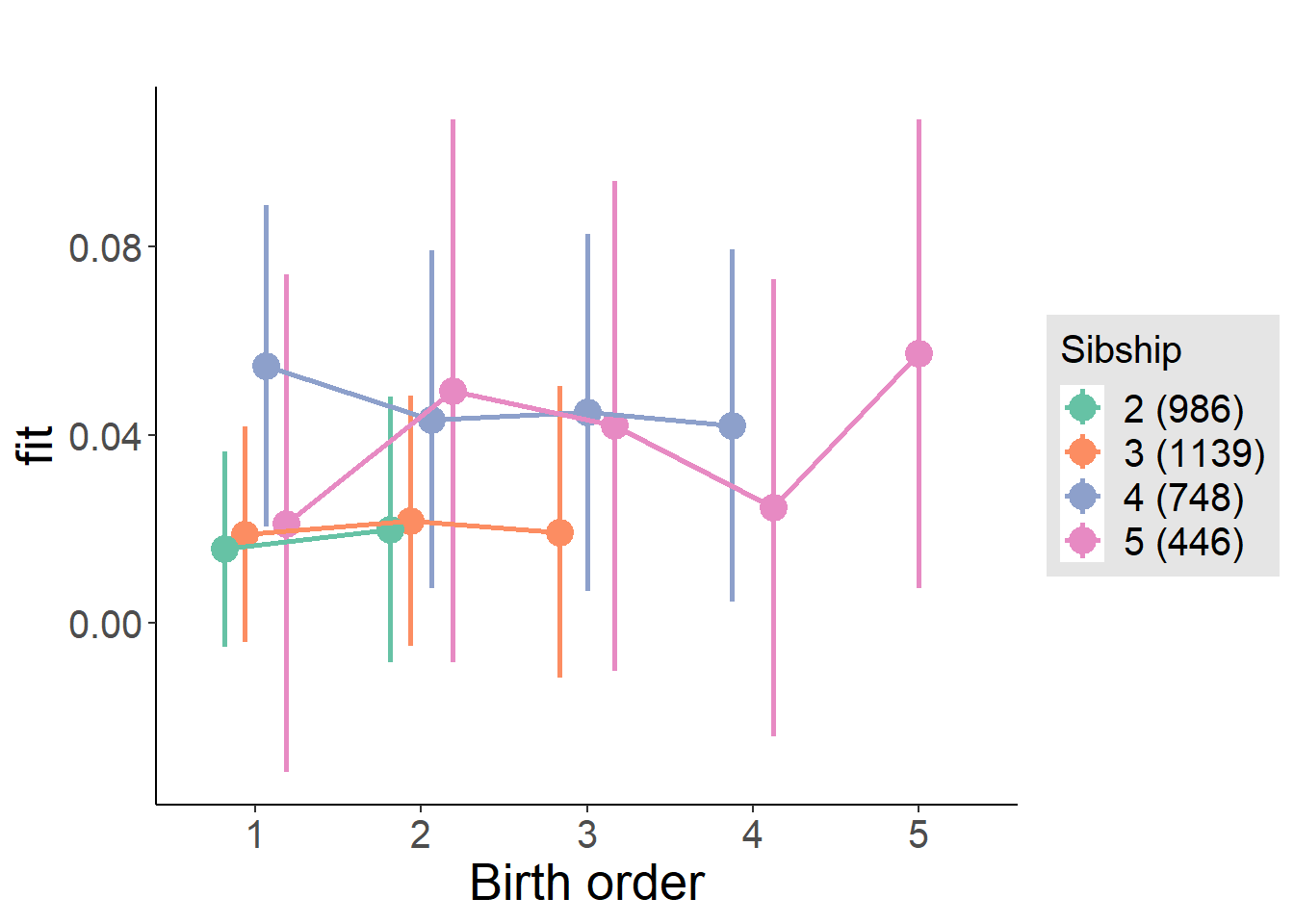
Model Comparison
###### Model 1 - Model 2
anova(m1_covariates_only, m2_birthorder_linear, m3_birthorder_nonlinear, m4_interaction)## refitting model(s) with ML (instead of REML)| Df | AIC | BIC | logLik | deviance | Chisq | Chi Df | Pr(>Chisq) |
|---|---|---|---|---|---|---|---|
| 10 | -2271 | -2210 | 1146 | -2291 | NA | NA | NA |
| 11 | -2269 | -2202 | 1146 | -2291 | 0.05045 | 1 | 0.8223 |
| 14 | -2265 | -2180 | 1147 | -2293 | 2.09 | 3 | 0.554 |
| 20 | -2255 | -2133 | 1148 | -2295 | 1.907 | 6 | 0.928 |
Maternal pregnancy order
outcome_preg_m1 <- update(m2_birthorder_linear, data = birthorder %>%
mutate(sibling_count = sibling_count_uterus_preg_factor,
birth_order_nonlinear = birthorder_uterus_preg_factor,
birth_order = birthorder_uterus_preg,
count_birth_order = count_birthorder_uterus_preg
) %>%
filter(sibling_count != "1"))
compare_models_markdown(outcome_preg_m1)Basic Model
Model Summary
m1_covariates_only <- update(m2_birthorder_linear, formula = . ~ . - birth_order)
tidy(m1_covariates_only, conf.int = T, conf.level = 0.995)| effect | group | term | estimate | std.error | statistic | df | p.value | conf.low | conf.high |
|---|---|---|---|---|---|---|---|---|---|
| fixed | NA | (Intercept) | 0.09531 | 0.1437 | 0.6634 | 3108 | 0.5071 | -0.308 | 0.4986 |
| fixed | NA | poly(age, 3, raw = TRUE)1 | -0.01133 | 0.01793 | -0.6318 | 3111 | 0.5276 | -0.06166 | 0.039 |
| fixed | NA | poly(age, 3, raw = TRUE)2 | 0.0004759 | 0.0007107 | 0.6697 | 3109 | 0.5031 | -0.001519 | 0.002471 |
| fixed | NA | poly(age, 3, raw = TRUE)3 | -0.000006334 | 0.000008915 | -0.7104 | 3101 | 0.4775 | -0.00003136 | 0.00001869 |
| fixed | NA | male | 0.02382 | 0.006131 | 3.885 | 3105 | 0.0001043 | 0.006612 | 0.04103 |
| fixed | NA | sibling_count3 | -0.002972 | 0.008136 | -0.3653 | 2565 | 0.7149 | -0.02581 | 0.01987 |
| fixed | NA | sibling_count4 | 0.02307 | 0.008802 | 2.62 | 2413 | 0.00884 | -0.001644 | 0.04777 |
| fixed | NA | sibling_count5 | 0.02403 | 0.009722 | 2.471 | 2185 | 0.01354 | -0.003265 | 0.05132 |
| ran_pars | mother_pidlink | sd__(Intercept) | 0.04101 | NA | NA | NA | NA | NA | NA |
| ran_pars | Residual | sd__Observation | 0.1662 | NA | NA | NA | NA | NA | NA |
Coefficient Plot
plot(allEffects(m1_covariates_only, confidence.level = 0.995))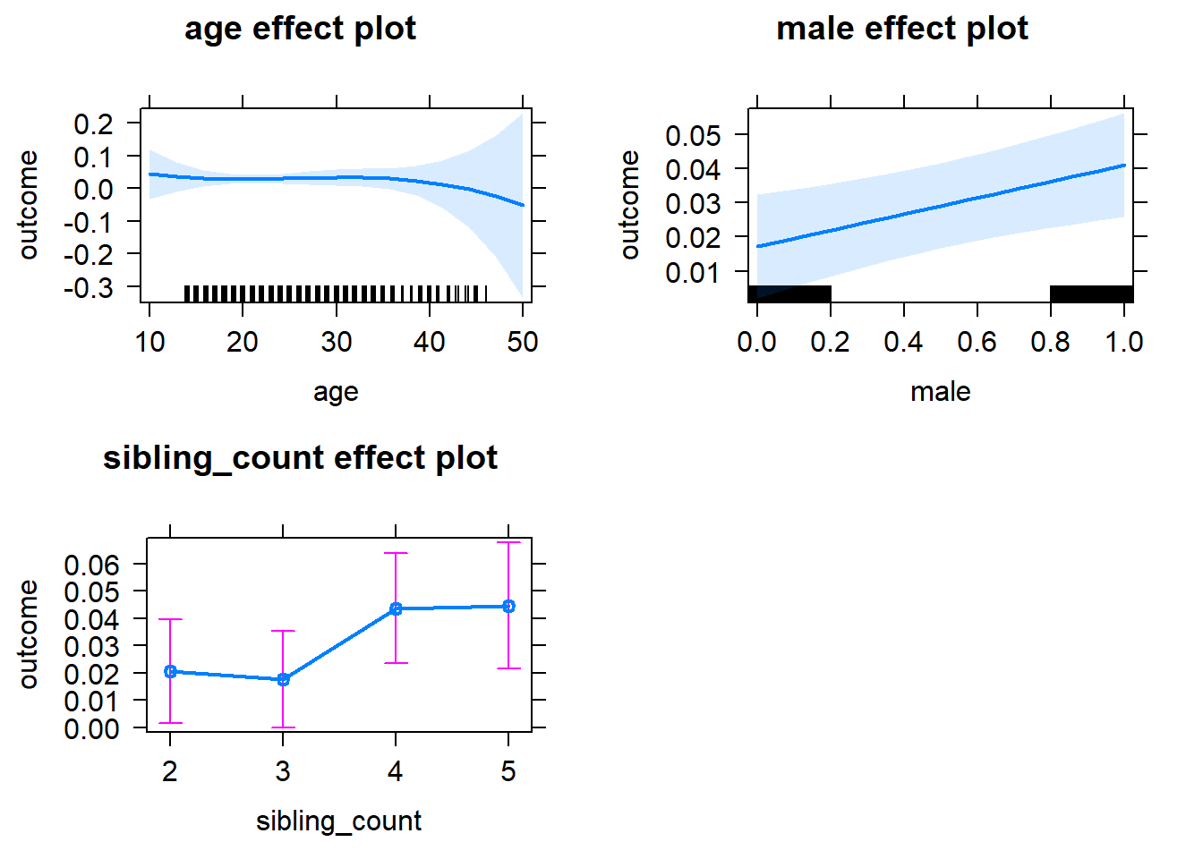
Add Birth Order Linear
Model Summary
tidy(m2_birthorder_linear, conf.int = T, conf.level = 0.995)| effect | group | term | estimate | std.error | statistic | df | p.value | conf.low | conf.high |
|---|---|---|---|---|---|---|---|---|---|
| fixed | NA | (Intercept) | 0.09804 | 0.1438 | 0.6818 | 3108 | 0.4954 | -0.3056 | 0.5017 |
| fixed | NA | birth_order | -0.001529 | 0.003188 | -0.4796 | 3100 | 0.6315 | -0.01048 | 0.007421 |
| fixed | NA | poly(age, 3, raw = TRUE)1 | -0.01142 | 0.01793 | -0.6368 | 3110 | 0.5243 | -0.06176 | 0.03892 |
| fixed | NA | poly(age, 3, raw = TRUE)2 | 0.00048 | 0.0007108 | 0.6753 | 3108 | 0.4995 | -0.001515 | 0.002475 |
| fixed | NA | poly(age, 3, raw = TRUE)3 | -0.000006398 | 0.000008917 | -0.7175 | 3100 | 0.4731 | -0.00003143 | 0.00001863 |
| fixed | NA | male | 0.02384 | 0.006132 | 3.887 | 3104 | 0.0001034 | 0.006625 | 0.04105 |
| fixed | NA | sibling_count3 | -0.002245 | 0.008277 | -0.2713 | 2584 | 0.7862 | -0.02548 | 0.02099 |
| fixed | NA | sibling_count4 | 0.02468 | 0.009426 | 2.618 | 2480 | 0.008894 | -0.00178 | 0.05114 |
| fixed | NA | sibling_count5 | 0.02658 | 0.01109 | 2.398 | 2398 | 0.01656 | -0.004535 | 0.0577 |
| ran_pars | mother_pidlink | sd__(Intercept) | 0.04116 | NA | NA | NA | NA | NA | NA |
| ran_pars | Residual | sd__Observation | 0.1662 | NA | NA | NA | NA | NA | NA |
Coefficient Plot
plot_birthorder2(m2_birthorder_linear, separate = FALSE)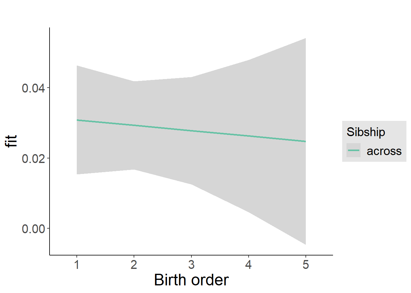
Add Birth Order Factor
Model Summary
m3_birthorder_nonlinear = update(m1_covariates_only, formula = . ~ . + birth_order_nonlinear)
tidy(m3_birthorder_nonlinear, conf.int = T, conf.level = 0.995)| effect | group | term | estimate | std.error | statistic | df | p.value | conf.low | conf.high |
|---|---|---|---|---|---|---|---|---|---|
| fixed | NA | (Intercept) | 0.09375 | 0.1439 | 0.6515 | 3106 | 0.5148 | -0.3102 | 0.4977 |
| fixed | NA | poly(age, 3, raw = TRUE)1 | -0.01133 | 0.01795 | -0.6314 | 3107 | 0.5278 | -0.06171 | 0.03905 |
| fixed | NA | poly(age, 3, raw = TRUE)2 | 0.0004761 | 0.0007113 | 0.6694 | 3104 | 0.5033 | -0.001521 | 0.002473 |
| fixed | NA | poly(age, 3, raw = TRUE)3 | -0.000006344 | 0.000008922 | -0.711 | 3095 | 0.4772 | -0.00003139 | 0.0000187 |
| fixed | NA | male | 0.024 | 0.006136 | 3.911 | 3101 | 0.00009392 | 0.006773 | 0.04122 |
| fixed | NA | sibling_count3 | -0.0009982 | 0.008439 | -0.1183 | 2640 | 0.9058 | -0.02469 | 0.02269 |
| fixed | NA | sibling_count4 | 0.02583 | 0.009595 | 2.692 | 2520 | 0.007156 | -0.001107 | 0.05276 |
| fixed | NA | sibling_count5 | 0.02749 | 0.01128 | 2.436 | 2379 | 0.01494 | -0.00419 | 0.05916 |
| fixed | NA | birth_order_nonlinear2 | 0.004655 | 0.007363 | 0.6323 | 2663 | 0.5272 | -0.01601 | 0.02532 |
| fixed | NA | birth_order_nonlinear3 | -0.008242 | 0.009483 | -0.8691 | 2972 | 0.3848 | -0.03486 | 0.01838 |
| fixed | NA | birth_order_nonlinear4 | -0.003501 | 0.01258 | -0.2783 | 3049 | 0.7808 | -0.03881 | 0.0318 |
| fixed | NA | birth_order_nonlinear5 | -0.001451 | 0.01903 | -0.07624 | 3071 | 0.9392 | -0.05486 | 0.05195 |
| ran_pars | mother_pidlink | sd__(Intercept) | 0.04085 | NA | NA | NA | NA | NA | NA |
| ran_pars | Residual | sd__Observation | 0.1663 | NA | NA | NA | NA | NA | NA |
Coefficient Plot
plot_birthorder(m3_birthorder_nonlinear, separate = FALSE)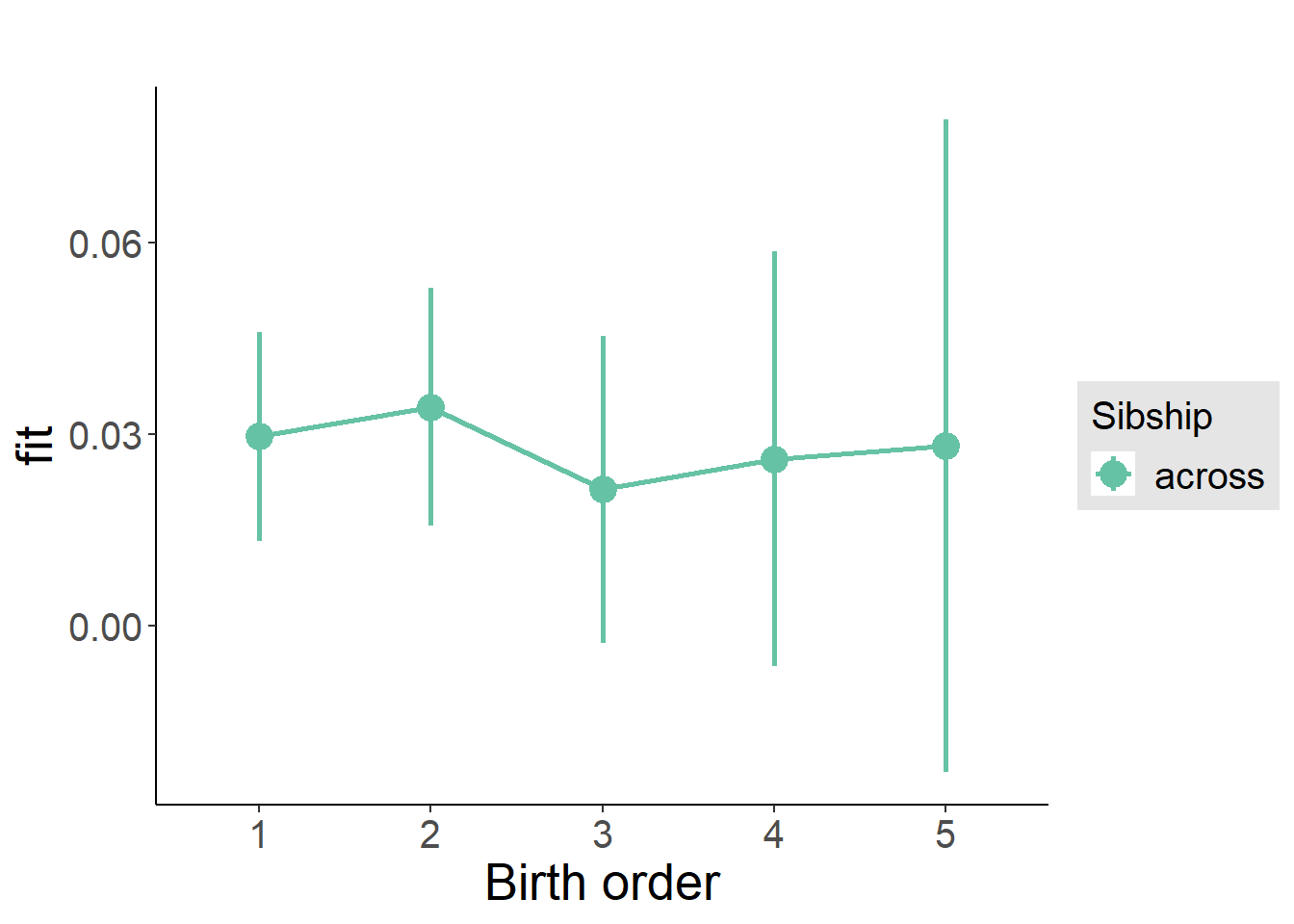
Add Interaction
Model Summary
m4_interaction = update(m3_birthorder_nonlinear, formula = . ~ . - birth_order_nonlinear - sibling_count + count_birth_order)
tidy(m4_interaction, conf.int = T, conf.level = 0.995)| effect | group | term | estimate | std.error | statistic | df | p.value | conf.low | conf.high |
|---|---|---|---|---|---|---|---|---|---|
| fixed | NA | (Intercept) | 0.09543 | 0.1441 | 0.6622 | 3100 | 0.5079 | -0.3091 | 0.5 |
| fixed | NA | poly(age, 3, raw = TRUE)1 | -0.0117 | 0.01797 | -0.6514 | 3101 | 0.5148 | -0.06213 | 0.03873 |
| fixed | NA | poly(age, 3, raw = TRUE)2 | 0.0004895 | 0.000712 | 0.6875 | 3097 | 0.4918 | -0.001509 | 0.002488 |
| fixed | NA | poly(age, 3, raw = TRUE)3 | -0.00000649 | 0.000008931 | -0.7267 | 3089 | 0.4675 | -0.00003156 | 0.00001858 |
| fixed | NA | male | 0.02385 | 0.006146 | 3.88 | 3096 | 0.0001066 | 0.006594 | 0.0411 |
| fixed | NA | count_birth_order2/2 | 0.009331 | 0.01252 | 0.7454 | 2762 | 0.4561 | -0.02581 | 0.04447 |
| fixed | NA | count_birth_order1/3 | 0.004077 | 0.01099 | 0.3711 | 3101 | 0.7106 | -0.02676 | 0.03491 |
| fixed | NA | count_birth_order2/3 | -0.00007272 | 0.01192 | -0.0061 | 3101 | 0.9951 | -0.03353 | 0.03339 |
| fixed | NA | count_birth_order3/3 | -0.006943 | 0.01332 | -0.5212 | 3100 | 0.6022 | -0.04433 | 0.03045 |
| fixed | NA | count_birth_order1/4 | 0.0228 | 0.01385 | 1.646 | 3101 | 0.09995 | -0.01609 | 0.06168 |
| fixed | NA | count_birth_order2/4 | 0.02987 | 0.01397 | 2.138 | 3101 | 0.03263 | -0.009353 | 0.06908 |
| fixed | NA | count_birth_order3/4 | 0.01873 | 0.01555 | 1.205 | 3097 | 0.2283 | -0.0249 | 0.06237 |
| fixed | NA | count_birth_order4/4 | 0.03272 | 0.01512 | 2.164 | 3100 | 0.03052 | -0.009715 | 0.07515 |
| fixed | NA | count_birth_order1/5 | 0.03131 | 0.0172 | 1.82 | 3101 | 0.06886 | -0.01698 | 0.0796 |
| fixed | NA | count_birth_order2/5 | 0.0482 | 0.01944 | 2.48 | 3095 | 0.0132 | -0.006361 | 0.1028 |
| fixed | NA | count_birth_order3/5 | 0.01967 | 0.01788 | 1.1 | 3099 | 0.2713 | -0.03051 | 0.06985 |
| fixed | NA | count_birth_order4/5 | 0.01146 | 0.0183 | 0.6262 | 3093 | 0.5312 | -0.03991 | 0.06284 |
| fixed | NA | count_birth_order5/5 | 0.02748 | 0.0179 | 1.535 | 3098 | 0.1249 | -0.02277 | 0.07774 |
| ran_pars | mother_pidlink | sd__(Intercept) | 0.03987 | NA | NA | NA | NA | NA | NA |
| ran_pars | Residual | sd__Observation | 0.1666 | NA | NA | NA | NA | NA | NA |
Coefficient Plot
plot_birthorder(m4_interaction)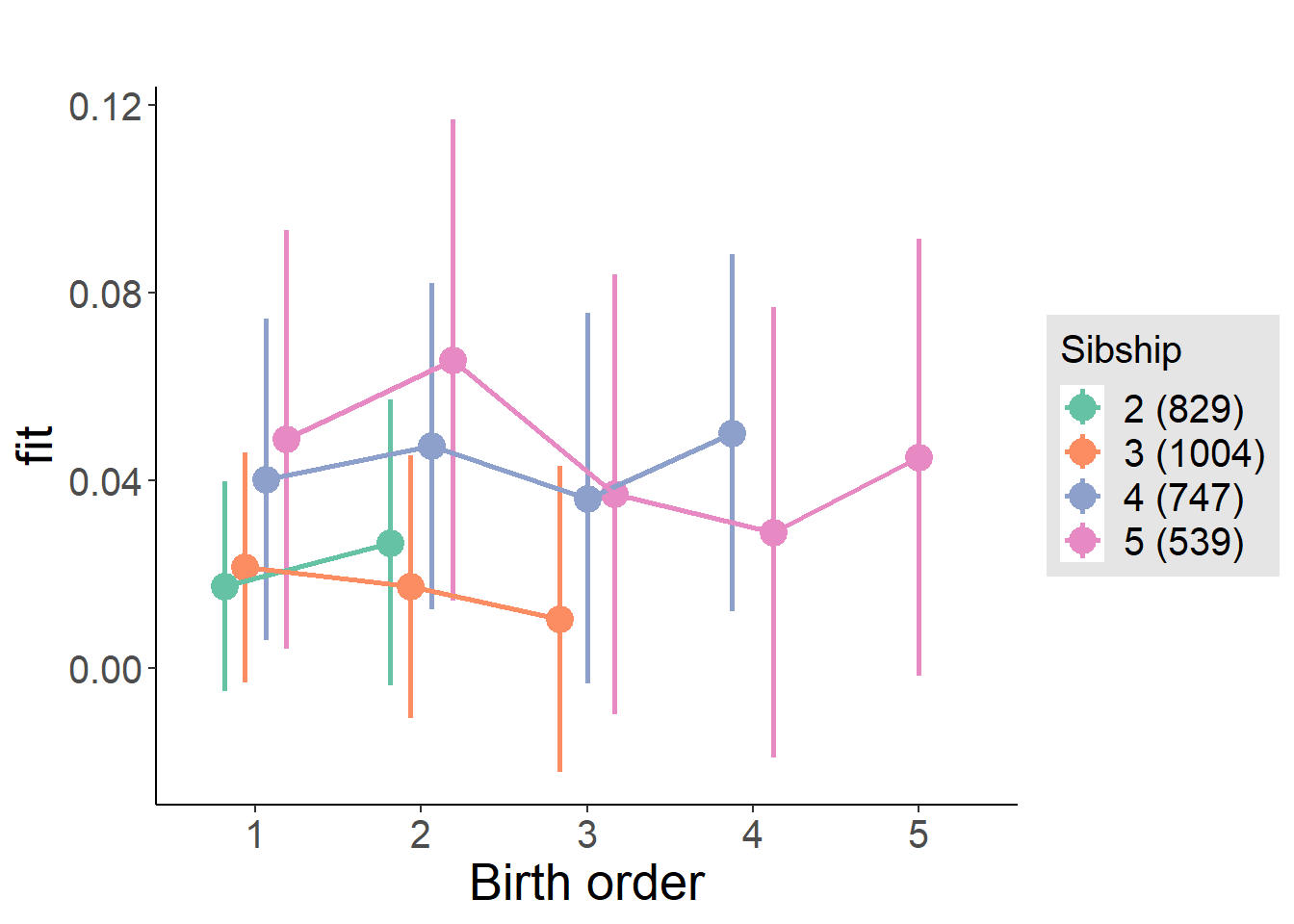
Model Comparison
###### Model 1 - Model 2
anova(m1_covariates_only, m2_birthorder_linear, m3_birthorder_nonlinear, m4_interaction)## refitting model(s) with ML (instead of REML)| Df | AIC | BIC | logLik | deviance | Chisq | Chi Df | Pr(>Chisq) |
|---|---|---|---|---|---|---|---|
| 10 | -2150 | -2090 | 1085 | -2170 | NA | NA | NA |
| 11 | -2149 | -2082 | 1085 | -2171 | 0.2296 | 1 | 0.6319 |
| 14 | -2144 | -2060 | 1086 | -2172 | 1.586 | 3 | 0.6625 |
| 20 | -2135 | -2014 | 1087 | -2175 | 2.7 | 6 | 0.8454 |
Parental full sibling order
outcome_parental_m1 <- update(m2_birthorder_linear, data = birthorder %>%
mutate(sibling_count = sibling_count_genes_factor,
birth_order_nonlinear = birthorder_genes_factor,
birth_order = birthorder_genes,
count_birth_order = count_birthorder_genes
) %>%
filter(sibling_count != "1"))
compare_models_markdown(outcome_parental_m1)Basic Model
Model Summary
m1_covariates_only <- update(m2_birthorder_linear, formula = . ~ . - birth_order)
tidy(m1_covariates_only, conf.int = T, conf.level = 0.995)| effect | group | term | estimate | std.error | statistic | df | p.value | conf.low | conf.high |
|---|---|---|---|---|---|---|---|---|---|
| fixed | NA | (Intercept) | 0.156 | 0.14 | 1.114 | 3277 | 0.2654 | -0.2371 | 0.5491 |
| fixed | NA | poly(age, 3, raw = TRUE)1 | -0.01887 | 0.01748 | -1.079 | 3283 | 0.2806 | -0.06794 | 0.03021 |
| fixed | NA | poly(age, 3, raw = TRUE)2 | 0.0007754 | 0.0006935 | 1.118 | 3285 | 0.2636 | -0.001171 | 0.002722 |
| fixed | NA | poly(age, 3, raw = TRUE)3 | -0.000009944 | 0.000008715 | -1.141 | 3282 | 0.254 | -0.00003441 | 0.00001452 |
| fixed | NA | male | 0.02102 | 0.005973 | 3.519 | 3265 | 0.0004396 | 0.004251 | 0.03778 |
| fixed | NA | sibling_count3 | 0.0004924 | 0.00758 | 0.06496 | 2707 | 0.9482 | -0.02079 | 0.02177 |
| fixed | NA | sibling_count4 | 0.02073 | 0.008548 | 2.425 | 2498 | 0.01537 | -0.003263 | 0.04473 |
| fixed | NA | sibling_count5 | 0.02588 | 0.01053 | 2.457 | 2355 | 0.01406 | -0.003681 | 0.05544 |
| ran_pars | mother_pidlink | sd__(Intercept) | 0.05616 | NA | NA | NA | NA | NA | NA |
| ran_pars | Residual | sd__Observation | 0.1623 | NA | NA | NA | NA | NA | NA |
Coefficient Plot
plot(allEffects(m1_covariates_only, confidence.level = 0.995))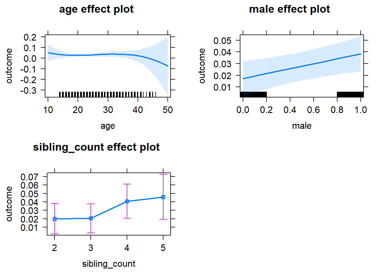
Add Birth Order Linear
Model Summary
tidy(m2_birthorder_linear, conf.int = T, conf.level = 0.995)| effect | group | term | estimate | std.error | statistic | df | p.value | conf.low | conf.high |
|---|---|---|---|---|---|---|---|---|---|
| fixed | NA | (Intercept) | 0.1552 | 0.1402 | 1.107 | 3278 | 0.2684 | -0.2384 | 0.5489 |
| fixed | NA | birth_order | 0.0003771 | 0.003285 | 0.1148 | 3236 | 0.9086 | -0.008844 | 0.009598 |
| fixed | NA | poly(age, 3, raw = TRUE)1 | -0.01884 | 0.01749 | -1.077 | 3282 | 0.2815 | -0.06792 | 0.03025 |
| fixed | NA | poly(age, 3, raw = TRUE)2 | 0.0007742 | 0.0006936 | 1.116 | 3284 | 0.2645 | -0.001173 | 0.002721 |
| fixed | NA | poly(age, 3, raw = TRUE)3 | -0.000009927 | 0.000008718 | -1.139 | 3281 | 0.2549 | -0.0000344 | 0.00001454 |
| fixed | NA | male | 0.02101 | 0.005974 | 3.517 | 3264 | 0.0004423 | 0.004242 | 0.03778 |
| fixed | NA | sibling_count3 | 0.0003212 | 0.007725 | 0.04158 | 2733 | 0.9668 | -0.02136 | 0.02201 |
| fixed | NA | sibling_count4 | 0.02032 | 0.009268 | 2.193 | 2614 | 0.02843 | -0.005695 | 0.04634 |
| fixed | NA | sibling_count5 | 0.02522 | 0.01199 | 2.103 | 2594 | 0.03553 | -0.008438 | 0.05888 |
| ran_pars | mother_pidlink | sd__(Intercept) | 0.05615 | NA | NA | NA | NA | NA | NA |
| ran_pars | Residual | sd__Observation | 0.1624 | NA | NA | NA | NA | NA | NA |
Coefficient Plot
plot_birthorder2(m2_birthorder_linear, separate = FALSE)
Add Birth Order Factor
Model Summary
m3_birthorder_nonlinear = update(m1_covariates_only, formula = . ~ . + birth_order_nonlinear)
tidy(m3_birthorder_nonlinear, conf.int = T, conf.level = 0.995)| effect | group | term | estimate | std.error | statistic | df | p.value | conf.low | conf.high |
|---|---|---|---|---|---|---|---|---|---|
| fixed | NA | (Intercept) | 0.1562 | 0.1404 | 1.112 | 3277 | 0.2661 | -0.238 | 0.5504 |
| fixed | NA | poly(age, 3, raw = TRUE)1 | -0.01903 | 0.01751 | -1.087 | 3280 | 0.2773 | -0.06819 | 0.03013 |
| fixed | NA | poly(age, 3, raw = TRUE)2 | 0.0007825 | 0.0006946 | 1.126 | 3281 | 0.26 | -0.001167 | 0.002732 |
| fixed | NA | poly(age, 3, raw = TRUE)3 | -0.00001004 | 0.000008728 | -1.15 | 3277 | 0.2503 | -0.00003454 | 0.00001447 |
| fixed | NA | male | 0.02108 | 0.005978 | 3.527 | 3261 | 0.0004261 | 0.004304 | 0.03786 |
| fixed | NA | sibling_count3 | 0.0006801 | 0.007883 | 0.08627 | 2791 | 0.9313 | -0.02145 | 0.02281 |
| fixed | NA | sibling_count4 | 0.02179 | 0.009461 | 2.303 | 2657 | 0.02133 | -0.004764 | 0.04835 |
| fixed | NA | sibling_count5 | 0.02467 | 0.01239 | 1.99 | 2600 | 0.0467 | -0.01013 | 0.05946 |
| fixed | NA | birth_order_nonlinear2 | 0.002625 | 0.007026 | 0.3736 | 2773 | 0.7087 | -0.0171 | 0.02235 |
| fixed | NA | birth_order_nonlinear3 | -0.0005137 | 0.009271 | -0.05541 | 3106 | 0.9558 | -0.02654 | 0.02551 |
| fixed | NA | birth_order_nonlinear4 | -0.003143 | 0.01297 | -0.2423 | 3173 | 0.8086 | -0.03956 | 0.03327 |
| fixed | NA | birth_order_nonlinear5 | 0.01182 | 0.0218 | 0.5421 | 3223 | 0.5878 | -0.04937 | 0.073 |
| ran_pars | mother_pidlink | sd__(Intercept) | 0.05586 | NA | NA | NA | NA | NA | NA |
| ran_pars | Residual | sd__Observation | 0.1625 | NA | NA | NA | NA | NA | NA |
Coefficient Plot
plot_birthorder(m3_birthorder_nonlinear, separate = FALSE)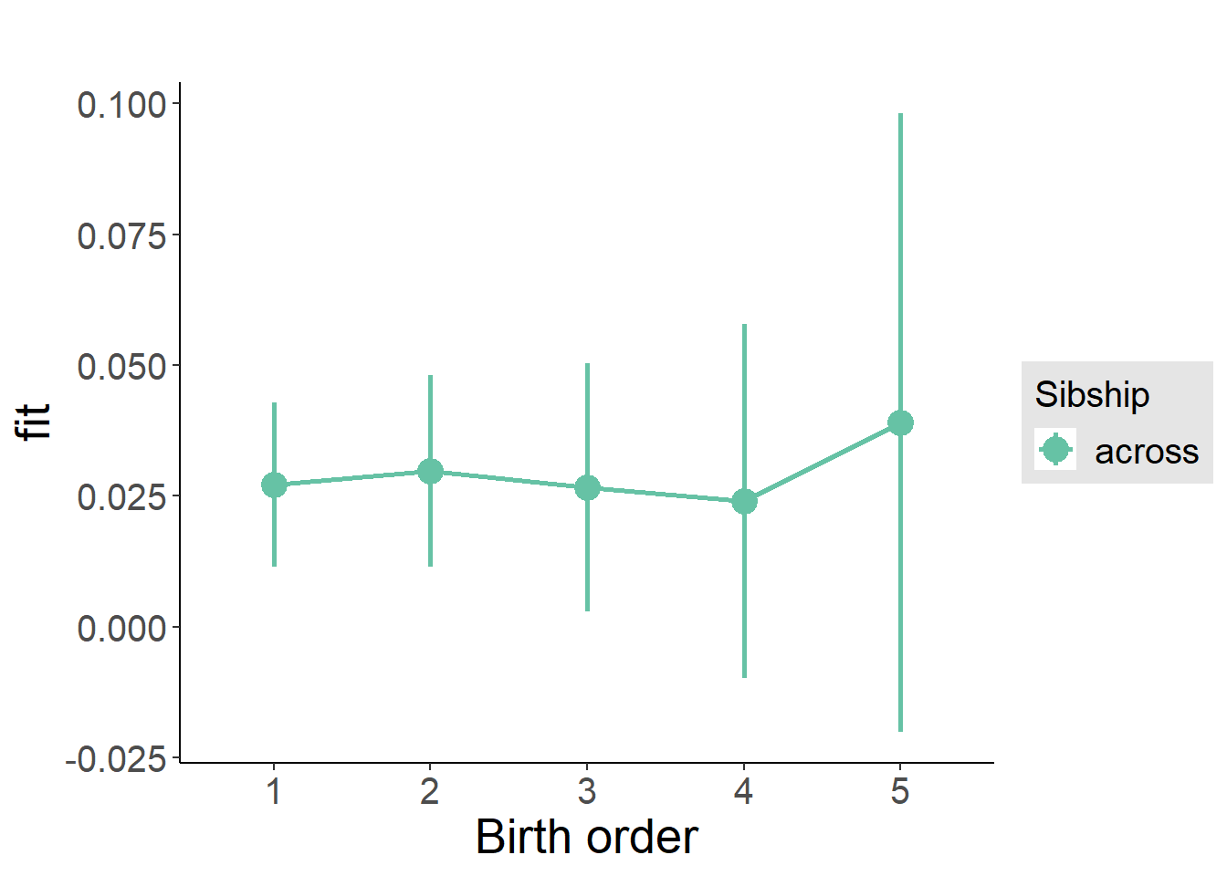
Add Interaction
Model Summary
m4_interaction = update(m3_birthorder_nonlinear, formula = . ~ . - birth_order_nonlinear - sibling_count + count_birth_order)
tidy(m4_interaction, conf.int = T, conf.level = 0.995)| effect | group | term | estimate | std.error | statistic | df | p.value | conf.low | conf.high |
|---|---|---|---|---|---|---|---|---|---|
| fixed | NA | (Intercept) | 0.1548 | 0.1406 | 1.101 | 3271 | 0.2709 | -0.2399 | 0.5496 |
| fixed | NA | poly(age, 3, raw = TRUE)1 | -0.01905 | 0.01753 | -1.086 | 3274 | 0.2775 | -0.06826 | 0.03017 |
| fixed | NA | poly(age, 3, raw = TRUE)2 | 0.0007824 | 0.0006954 | 1.125 | 3275 | 0.2606 | -0.00117 | 0.002734 |
| fixed | NA | poly(age, 3, raw = TRUE)3 | -0.00001003 | 0.000008738 | -1.148 | 3271 | 0.2509 | -0.00003456 | 0.00001449 |
| fixed | NA | male | 0.02103 | 0.005987 | 3.512 | 3256 | 0.0004501 | 0.004223 | 0.03783 |
| fixed | NA | count_birth_order2/2 | 0.007624 | 0.01112 | 0.6858 | 2900 | 0.4929 | -0.02358 | 0.03883 |
| fixed | NA | count_birth_order1/3 | 0.003736 | 0.01014 | 0.3685 | 3274 | 0.7125 | -0.02472 | 0.03219 |
| fixed | NA | count_birth_order2/3 | 0.002889 | 0.01128 | 0.2561 | 3273 | 0.7979 | -0.02877 | 0.03455 |
| fixed | NA | count_birth_order3/3 | 0.002055 | 0.0124 | 0.1657 | 3273 | 0.8684 | -0.03275 | 0.03686 |
| fixed | NA | count_birth_order1/4 | 0.02963 | 0.01373 | 2.158 | 3274 | 0.03097 | -0.008906 | 0.06817 |
| fixed | NA | count_birth_order2/4 | 0.02198 | 0.01415 | 1.553 | 3269 | 0.1205 | -0.01775 | 0.06171 |
| fixed | NA | count_birth_order3/4 | 0.02018 | 0.01454 | 1.387 | 3264 | 0.1654 | -0.02065 | 0.06101 |
| fixed | NA | count_birth_order4/4 | 0.02042 | 0.01486 | 1.374 | 3271 | 0.1695 | -0.02128 | 0.06211 |
| fixed | NA | count_birth_order1/5 | 0.01691 | 0.01982 | 0.8531 | 3272 | 0.3937 | -0.03873 | 0.07255 |
| fixed | NA | count_birth_order2/5 | 0.03535 | 0.02254 | 1.569 | 3249 | 0.1168 | -0.02791 | 0.09861 |
| fixed | NA | count_birth_order3/5 | 0.03142 | 0.02058 | 1.527 | 3262 | 0.1269 | -0.02635 | 0.0892 |
| fixed | NA | count_birth_order4/5 | 0.02316 | 0.01923 | 1.204 | 3259 | 0.2285 | -0.03082 | 0.07714 |
| fixed | NA | count_birth_order5/5 | 0.0383 | 0.01998 | 1.917 | 3269 | 0.05538 | -0.01779 | 0.09439 |
| ran_pars | mother_pidlink | sd__(Intercept) | 0.05551 | NA | NA | NA | NA | NA | NA |
| ran_pars | Residual | sd__Observation | 0.1628 | NA | NA | NA | NA | NA | NA |
Coefficient Plot
plot_birthorder(m4_interaction)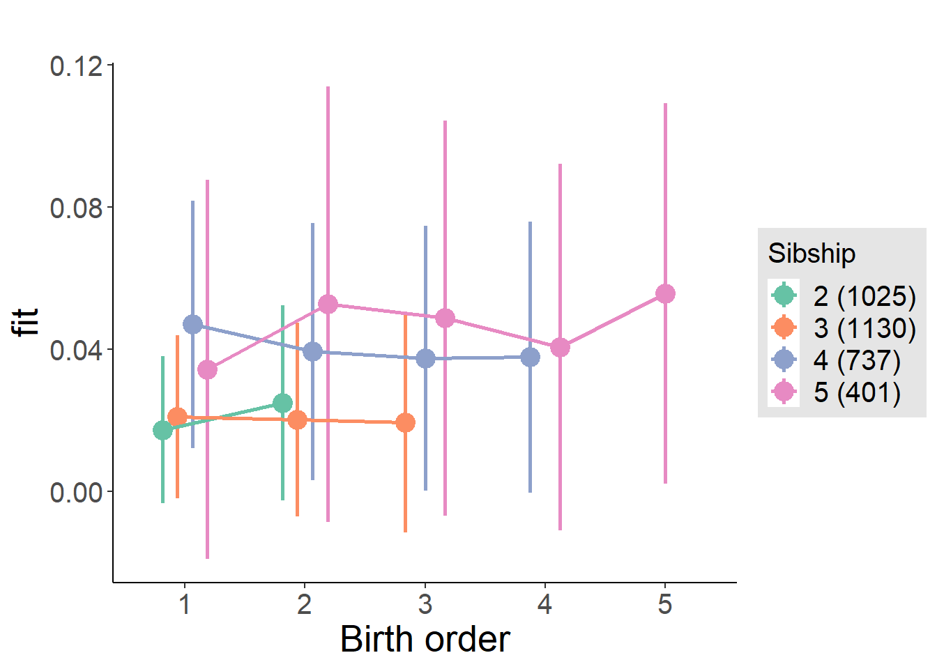
Model Comparison
###### Model 1 - Model 2
anova(m1_covariates_only, m2_birthorder_linear, m3_birthorder_nonlinear, m4_interaction)## refitting model(s) with ML (instead of REML)| Df | AIC | BIC | logLik | deviance | Chisq | Chi Df | Pr(>Chisq) |
|---|---|---|---|---|---|---|---|
| 10 | -2255 | -2194 | 1137 | -2275 | NA | NA | NA |
| 11 | -2253 | -2186 | 1137 | -2275 | 0.01335 | 1 | 0.908 |
| 14 | -2247 | -2162 | 1138 | -2275 | 0.6087 | 3 | 0.8944 |
| 20 | -2237 | -2115 | 1138 | -2277 | 1.169 | 6 | 0.9784 |
Compare birth order specifications
library(coefplot)
multiplot(outcome_naive_m1, outcome_preg_m1, outcome_uterus_m1, outcome_parental_m1, dodgeHeight = 0.6,
intercept = FALSE)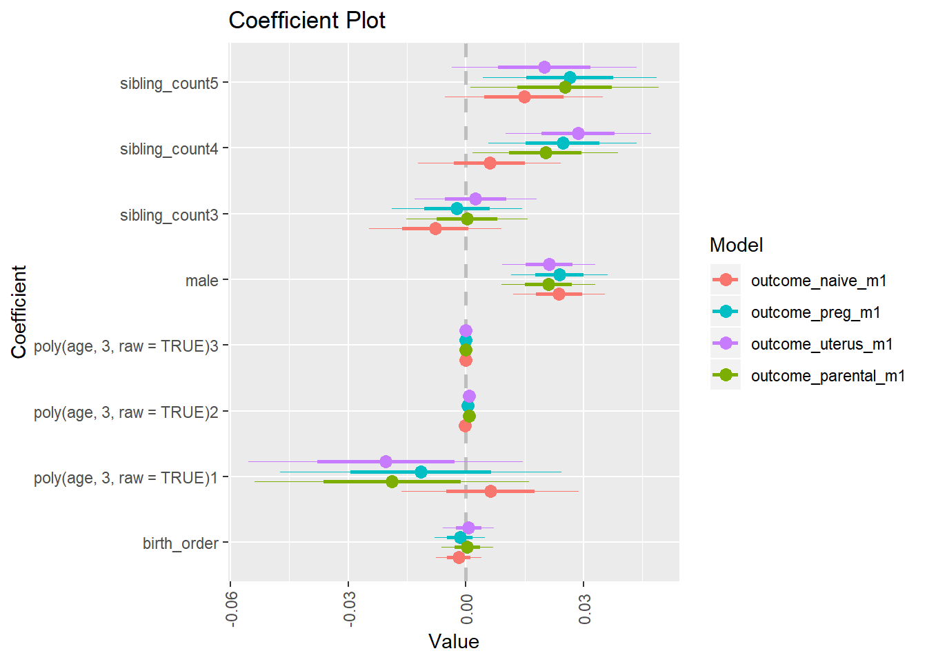
Attended School
birthorder <- birthorder %>% mutate(outcome = attended_school)
model = lmer(outcome ~ birth_order + poly(age, 3, raw = TRUE) + male + sibling_count + (1 | mother_pidlink),
data = birthorder)
compare_birthorder_specs(model)Naive birth order
outcome_naive_m1 <- update(m2_birthorder_linear, data = birthorder %>%
mutate(sibling_count = sibling_count_naive_factor,
birth_order_nonlinear = birthorder_naive_factor,
birth_order = birthorder_naive,
count_birth_order = count_birthorder_naive) %>%
filter(sibling_count != "1"))
compare_models_markdown(outcome_naive_m1)Basic Model
Model Summary
m1_covariates_only <- update(m2_birthorder_linear, formula = . ~ . - birth_order)
tidy(m1_covariates_only, conf.int = T, conf.level = 0.995)| effect | group | term | estimate | std.error | statistic | df | p.value | conf.low | conf.high |
|---|---|---|---|---|---|---|---|---|---|
| fixed | NA | (Intercept) | 0.914 | 0.0215 | 42.51 | 7401 | 0 | 0.8536 | 0.9743 |
| fixed | NA | poly(age, 3, raw = TRUE)1 | 0.007969 | 0.002044 | 3.898 | 7331 | 0.00009796 | 0.00223 | 0.01371 |
| fixed | NA | poly(age, 3, raw = TRUE)2 | -0.000214 | 0.000059 | -3.627 | 7243 | 0.0002885 | -0.0003796 | -0.00004839 |
| fixed | NA | poly(age, 3, raw = TRUE)3 | 0.000001249 | 0.0000005279 | 2.366 | 7172 | 0.01801 | -0.0000002329 | 0.000002731 |
| fixed | NA | male | 0.005467 | 0.00257 | 2.127 | 7488 | 0.03347 | -0.001748 | 0.01268 |
| fixed | NA | sibling_count3 | -0.0007012 | 0.003722 | -0.1884 | 5946 | 0.8506 | -0.01115 | 0.009747 |
| fixed | NA | sibling_count4 | -0.0009832 | 0.003837 | -0.2562 | 5482 | 0.7978 | -0.01175 | 0.009788 |
| fixed | NA | sibling_count5 | 0.002998 | 0.004015 | 0.7467 | 5028 | 0.4553 | -0.008272 | 0.01427 |
| ran_pars | mother_pidlink | sd__(Intercept) | 0.03849 | NA | NA | NA | NA | NA | NA |
| ran_pars | Residual | sd__Observation | 0.1057 | NA | NA | NA | NA | NA | NA |
Coefficient Plot
plot(allEffects(m1_covariates_only, confidence.level = 0.995))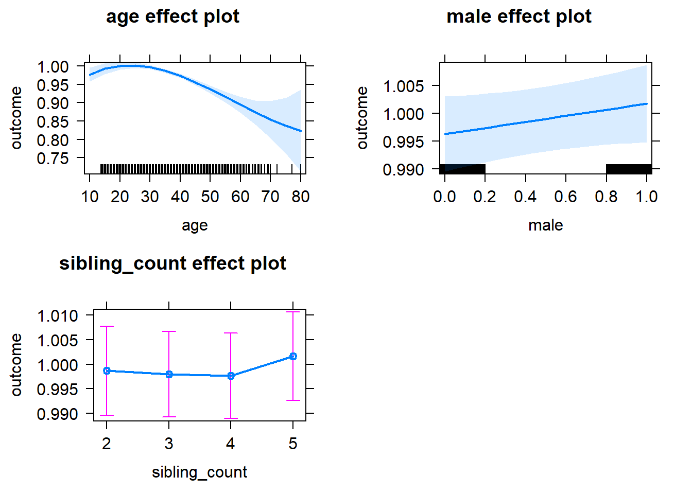
Add Birth Order Linear
Model Summary
tidy(m2_birthorder_linear, conf.int = T, conf.level = 0.995)| effect | group | term | estimate | std.error | statistic | df | p.value | conf.low | conf.high |
|---|---|---|---|---|---|---|---|---|---|
| fixed | NA | (Intercept) | 0.9131 | 0.0215 | 42.46 | 7394 | 0 | 0.8527 | 0.9734 |
| fixed | NA | birth_order | 0.002322 | 0.001279 | 1.815 | 6837 | 0.06962 | -0.00127 | 0.005913 |
| fixed | NA | poly(age, 3, raw = TRUE)1 | 0.00774 | 0.002048 | 3.779 | 7345 | 0.0001587 | 0.001991 | 0.01349 |
| fixed | NA | poly(age, 3, raw = TRUE)2 | -0.000208 | 0.00005908 | -3.521 | 7252 | 0.0004328 | -0.0003739 | -0.00004217 |
| fixed | NA | poly(age, 3, raw = TRUE)3 | 0.000001209 | 0.0000005283 | 2.289 | 7178 | 0.02209 | -0.0000002735 | 0.000002692 |
| fixed | NA | male | 0.005399 | 0.00257 | 2.101 | 7486 | 0.03571 | -0.001816 | 0.01261 |
| fixed | NA | sibling_count3 | -0.001528 | 0.00375 | -0.4075 | 6054 | 0.6837 | -0.01205 | 0.008997 |
| fixed | NA | sibling_count4 | -0.002894 | 0.003979 | -0.7273 | 5939 | 0.4671 | -0.01406 | 0.008275 |
| fixed | NA | sibling_count5 | -0.00006896 | 0.004356 | -0.01583 | 5953 | 0.9874 | -0.0123 | 0.01216 |
| ran_pars | mother_pidlink | sd__(Intercept) | 0.03851 | NA | NA | NA | NA | NA | NA |
| ran_pars | Residual | sd__Observation | 0.1057 | NA | NA | NA | NA | NA | NA |
Coefficient Plot
plot_birthorder2(m2_birthorder_linear, separate = FALSE)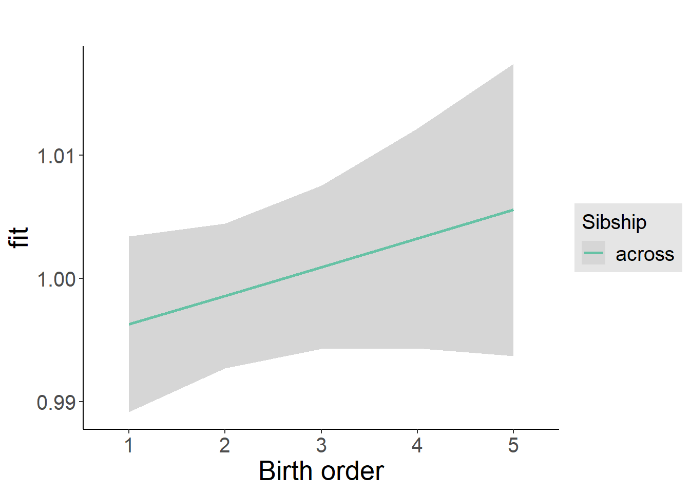
Add Birth Order Factor
Model Summary
m3_birthorder_nonlinear = update(m1_covariates_only, formula = . ~ . + birth_order_nonlinear)
tidy(m3_birthorder_nonlinear, conf.int = T, conf.level = 0.995)| effect | group | term | estimate | std.error | statistic | df | p.value | conf.low | conf.high |
|---|---|---|---|---|---|---|---|---|---|
| fixed | NA | (Intercept) | 0.9116 | 0.02155 | 42.3 | 7407 | 0 | 0.8511 | 0.9721 |
| fixed | NA | poly(age, 3, raw = TRUE)1 | 0.007886 | 0.002048 | 3.849 | 7339 | 0.0001194 | 0.002135 | 0.01364 |
| fixed | NA | poly(age, 3, raw = TRUE)2 | -0.0002142 | 0.00005911 | -3.623 | 7239 | 0.0002928 | -0.0003801 | -0.00004826 |
| fixed | NA | poly(age, 3, raw = TRUE)3 | 0.00000128 | 0.0000005288 | 2.421 | 7158 | 0.01551 | -0.0000002043 | 0.000002764 |
| fixed | NA | male | 0.005402 | 0.002569 | 2.102 | 7482 | 0.03555 | -0.00181 | 0.01261 |
| fixed | NA | sibling_count3 | -0.001566 | 0.003806 | -0.4114 | 6228 | 0.6808 | -0.01225 | 0.009118 |
| fixed | NA | sibling_count4 | -0.002531 | 0.004042 | -0.6262 | 6132 | 0.5312 | -0.01388 | 0.008814 |
| fixed | NA | sibling_count5 | 0.001566 | 0.004396 | 0.3562 | 6090 | 0.7217 | -0.01077 | 0.01391 |
| fixed | NA | birth_order_nonlinear2 | 0.01023 | 0.003037 | 3.368 | 6721 | 0.000761 | 0.001704 | 0.01875 |
| fixed | NA | birth_order_nonlinear3 | 0.006807 | 0.003889 | 1.75 | 6680 | 0.08011 | -0.004109 | 0.01772 |
| fixed | NA | birth_order_nonlinear4 | 0.006857 | 0.00509 | 1.347 | 6691 | 0.178 | -0.007432 | 0.02115 |
| fixed | NA | birth_order_nonlinear5 | 0.00418 | 0.00747 | 0.5596 | 6609 | 0.5758 | -0.01679 | 0.02515 |
| ran_pars | mother_pidlink | sd__(Intercept) | 0.03863 | NA | NA | NA | NA | NA | NA |
| ran_pars | Residual | sd__Observation | 0.1056 | NA | NA | NA | NA | NA | NA |
Coefficient Plot
plot_birthorder(m3_birthorder_nonlinear, separate = FALSE)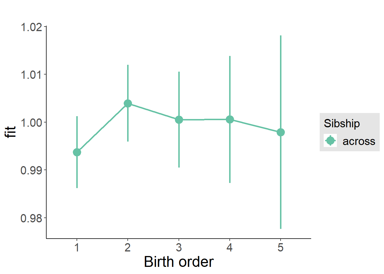
Add Interaction
Model Summary
m4_interaction = update(m3_birthorder_nonlinear, formula = . ~ . - birth_order_nonlinear - sibling_count + count_birth_order)
tidy(m4_interaction, conf.int = T, conf.level = 0.995)| effect | group | term | estimate | std.error | statistic | df | p.value | conf.low | conf.high |
|---|---|---|---|---|---|---|---|---|---|
| fixed | NA | (Intercept) | 0.9099 | 0.0216 | 42.12 | 7407 | 0 | 0.8493 | 0.9705 |
| fixed | NA | poly(age, 3, raw = TRUE)1 | 0.007873 | 0.002049 | 3.842 | 7335 | 0.000123 | 0.002121 | 0.01363 |
| fixed | NA | poly(age, 3, raw = TRUE)2 | -0.0002143 | 0.00005913 | -3.624 | 7234 | 0.0002926 | -0.0003802 | -0.00004828 |
| fixed | NA | poly(age, 3, raw = TRUE)3 | 0.000001284 | 0.0000005289 | 2.427 | 7150 | 0.01523 | -0.0000002008 | 0.000002769 |
| fixed | NA | male | 0.005426 | 0.00257 | 2.111 | 7476 | 0.03479 | -0.001789 | 0.01264 |
| fixed | NA | count_birth_order2/2 | 0.01558 | 0.005183 | 3.005 | 6670 | 0.002663 | 0.001028 | 0.03013 |
| fixed | NA | count_birth_order1/3 | 0.003308 | 0.004924 | 0.6718 | 7532 | 0.5017 | -0.01051 | 0.01713 |
| fixed | NA | count_birth_order2/3 | 0.007013 | 0.005508 | 1.273 | 7547 | 0.203 | -0.008448 | 0.02247 |
| fixed | NA | count_birth_order3/3 | 0.00626 | 0.006146 | 1.018 | 7552 | 0.3085 | -0.01099 | 0.02351 |
| fixed | NA | count_birth_order1/4 | -0.001249 | 0.005578 | -0.2239 | 7547 | 0.8228 | -0.01691 | 0.01441 |
| fixed | NA | count_birth_order2/4 | 0.008736 | 0.005935 | 1.472 | 7551 | 0.1411 | -0.007925 | 0.0254 |
| fixed | NA | count_birth_order3/4 | 0.007827 | 0.006441 | 1.215 | 7551 | 0.2243 | -0.01025 | 0.02591 |
| fixed | NA | count_birth_order4/4 | 0.007133 | 0.006763 | 1.055 | 7548 | 0.2916 | -0.01185 | 0.02612 |
| fixed | NA | count_birth_order1/5 | 0.003778 | 0.006386 | 0.5916 | 7552 | 0.5542 | -0.01415 | 0.0217 |
| fixed | NA | count_birth_order2/5 | 0.01494 | 0.00674 | 2.216 | 7549 | 0.02671 | -0.003983 | 0.03386 |
| fixed | NA | count_birth_order3/5 | 0.009701 | 0.006895 | 1.407 | 7546 | 0.1595 | -0.009654 | 0.02906 |
| fixed | NA | count_birth_order4/5 | 0.009395 | 0.007387 | 1.272 | 7535 | 0.2035 | -0.01134 | 0.03013 |
| fixed | NA | count_birth_order5/5 | 0.007711 | 0.007527 | 1.024 | 7533 | 0.3057 | -0.01342 | 0.02884 |
| ran_pars | mother_pidlink | sd__(Intercept) | 0.03861 | NA | NA | NA | NA | NA | NA |
| ran_pars | Residual | sd__Observation | 0.1056 | NA | NA | NA | NA | NA | NA |
Coefficient Plot
plot_birthorder(m4_interaction)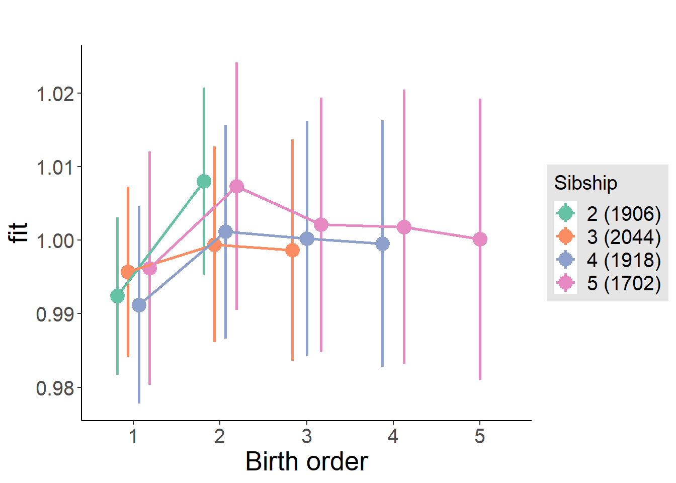
Model Comparison
###### Model 1 - Model 2
anova(m1_covariates_only, m2_birthorder_linear, m3_birthorder_nonlinear, m4_interaction)## refitting model(s) with ML (instead of REML)| Df | AIC | BIC | logLik | deviance | Chisq | Chi Df | Pr(>Chisq) |
|---|---|---|---|---|---|---|---|
| 10 | -11631 | -11562 | 5826 | -11651 | NA | NA | NA |
| 11 | -11633 | -11557 | 5827 | -11655 | 3.295 | 1 | 0.06949 |
| 14 | -11635 | -11538 | 5832 | -11663 | 8.559 | 3 | 0.03576 |
| 20 | -11626 | -11487 | 5833 | -11666 | 2.725 | 6 | 0.8425 |
Maternal birth order
outcome_uterus_m1 <- update(m2_birthorder_linear, data = birthorder %>%
mutate(sibling_count = sibling_count_uterus_alive_factor,
birth_order_nonlinear = birthorder_uterus_alive_factor,
birth_order = birthorder_uterus_alive,
count_birth_order = count_birthorder_uterus_alive) %>%
filter(sibling_count != "1"))## boundary (singular) fit: see ?isSingularcompare_models_markdown(outcome_uterus_m1)Basic Model
Model Summary
m1_covariates_only <- update(m2_birthorder_linear, formula = . ~ . - birth_order)## boundary (singular) fit: see ?isSingulartidy(m1_covariates_only, conf.int = T, conf.level = 0.995)| effect | group | term | estimate | std.error | statistic | df | p.value | conf.low | conf.high |
|---|---|---|---|---|---|---|---|---|---|
| fixed | NA | (Intercept) | 0.9676 | 0.03025 | 31.98 | 4744 | 2.082e-203 | 0.8827 | 1.053 |
| fixed | NA | poly(age, 3, raw = TRUE)1 | 0.003197 | 0.00353 | 0.9058 | 4744 | 0.3651 | -0.006711 | 0.01311 |
| fixed | NA | poly(age, 3, raw = TRUE)2 | -0.0001046 | 0.0001301 | -0.8042 | 4744 | 0.4213 | -0.0004698 | 0.0002605 |
| fixed | NA | poly(age, 3, raw = TRUE)3 | 0.000001122 | 0.000001525 | 0.7362 | 4744 | 0.4616 | -0.000003157 | 0.000005402 |
| fixed | NA | male | -0.001234 | 0.00163 | -0.7572 | 4744 | 0.449 | -0.00581 | 0.003341 |
| fixed | NA | sibling_count3 | -0.0004113 | 0.002153 | -0.191 | 4744 | 0.8485 | -0.006456 | 0.005634 |
| fixed | NA | sibling_count4 | -0.001407 | 0.002304 | -0.6108 | 4744 | 0.5414 | -0.007875 | 0.00506 |
| fixed | NA | sibling_count5 | -0.003486 | 0.002629 | -1.326 | 4744 | 0.1848 | -0.01086 | 0.003892 |
| ran_pars | mother_pidlink | sd__(Intercept) | 0 | NA | NA | NA | NA | NA | NA |
| ran_pars | Residual | sd__Observation | 0.05611 | NA | NA | NA | NA | NA | NA |
Coefficient Plot
plot(allEffects(m1_covariates_only, confidence.level = 0.995))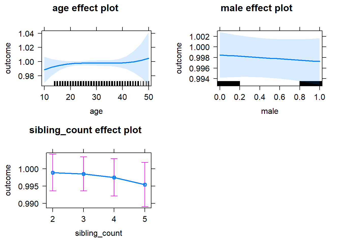
Add Birth Order Linear
Model Summary
tidy(m2_birthorder_linear, conf.int = T, conf.level = 0.995)| effect | group | term | estimate | std.error | statistic | df | p.value | conf.low | conf.high |
|---|---|---|---|---|---|---|---|---|---|
| fixed | NA | (Intercept) | 0.9655 | 0.03029 | 31.88 | 4743 | 3.321e-202 | 0.8805 | 1.051 |
| fixed | NA | birth_order | 0.001181 | 0.0008655 | 1.365 | 4743 | 0.1723 | -0.001248 | 0.003611 |
| fixed | NA | poly(age, 3, raw = TRUE)1 | 0.003281 | 0.00353 | 0.9293 | 4743 | 0.3528 | -0.006629 | 0.01319 |
| fixed | NA | poly(age, 3, raw = TRUE)2 | -0.0001092 | 0.0001301 | -0.8389 | 4743 | 0.4016 | -0.0004744 | 0.0002561 |
| fixed | NA | poly(age, 3, raw = TRUE)3 | 0.000001199 | 0.000001525 | 0.7858 | 4743 | 0.432 | -0.000003083 | 0.000005481 |
| fixed | NA | male | -0.001269 | 0.00163 | -0.7783 | 4743 | 0.4365 | -0.005844 | 0.003307 |
| fixed | NA | sibling_count3 | -0.0009595 | 0.00219 | -0.438 | 4743 | 0.6614 | -0.007108 | 0.005189 |
| fixed | NA | sibling_count4 | -0.002635 | 0.002473 | -1.065 | 4743 | 0.2868 | -0.009577 | 0.004307 |
| fixed | NA | sibling_count5 | -0.005526 | 0.003023 | -1.828 | 4743 | 0.06764 | -0.01401 | 0.002961 |
| ran_pars | mother_pidlink | sd__(Intercept) | 0 | NA | NA | NA | NA | NA | NA |
| ran_pars | Residual | sd__Observation | 0.05611 | NA | NA | NA | NA | NA | NA |
Coefficient Plot
plot_birthorder2(m2_birthorder_linear, separate = FALSE)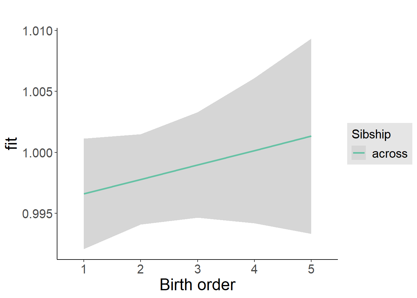
Add Birth Order Factor
Model Summary
m3_birthorder_nonlinear = update(m1_covariates_only, formula = . ~ . + birth_order_nonlinear)## boundary (singular) fit: see ?isSingulartidy(m3_birthorder_nonlinear, conf.int = T, conf.level = 0.995)| effect | group | term | estimate | std.error | statistic | df | p.value | conf.low | conf.high |
|---|---|---|---|---|---|---|---|---|---|
| fixed | NA | (Intercept) | 0.9718 | 0.03028 | 32.09 | 4740 | 1.099e-204 | 0.8868 | 1.057 |
| fixed | NA | poly(age, 3, raw = TRUE)1 | 0.002929 | 0.003529 | 0.8299 | 4740 | 0.4066 | -0.006978 | 0.01284 |
| fixed | NA | poly(age, 3, raw = TRUE)2 | -0.00009641 | 0.0001301 | -0.741 | 4740 | 0.4587 | -0.0004616 | 0.0002688 |
| fixed | NA | poly(age, 3, raw = TRUE)3 | 0.000001056 | 0.000001525 | 0.6924 | 4740 | 0.4887 | -0.000003225 | 0.000005337 |
| fixed | NA | male | -0.001339 | 0.001629 | -0.822 | 4740 | 0.4111 | -0.005911 | 0.003233 |
| fixed | NA | sibling_count3 | -0.001289 | 0.002227 | -0.5787 | 4740 | 0.5628 | -0.007541 | 0.004963 |
| fixed | NA | sibling_count4 | -0.00314 | 0.002512 | -1.25 | 4740 | 0.2113 | -0.01019 | 0.00391 |
| fixed | NA | sibling_count5 | -0.007082 | 0.003077 | -2.302 | 4740 | 0.02139 | -0.01572 | 0.001555 |
| fixed | NA | birth_order_nonlinear2 | -0.00492 | 0.001973 | -2.493 | 4740 | 0.0127 | -0.01046 | 0.0006195 |
| fixed | NA | birth_order_nonlinear3 | 0.003382 | 0.002506 | 1.349 | 4740 | 0.1773 | -0.003653 | 0.01042 |
| fixed | NA | birth_order_nonlinear4 | 0.002613 | 0.003372 | 0.7749 | 4740 | 0.4385 | -0.006852 | 0.01208 |
| fixed | NA | birth_order_nonlinear5 | 0.007239 | 0.005303 | 1.365 | 4740 | 0.1723 | -0.007647 | 0.02212 |
| ran_pars | mother_pidlink | sd__(Intercept) | 0 | NA | NA | NA | NA | NA | NA |
| ran_pars | Residual | sd__Observation | 0.05605 | NA | NA | NA | NA | NA | NA |
Coefficient Plot
plot_birthorder(m3_birthorder_nonlinear, separate = FALSE)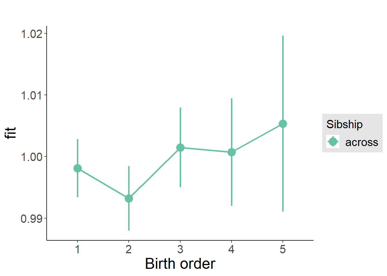
Add Interaction
Model Summary
m4_interaction = update(m3_birthorder_nonlinear, formula = . ~ . - birth_order_nonlinear - sibling_count + count_birth_order)## boundary (singular) fit: see ?isSingulartidy(m4_interaction, conf.int = T, conf.level = 0.995)| effect | group | term | estimate | std.error | statistic | df | p.value | conf.low | conf.high |
|---|---|---|---|---|---|---|---|---|---|
| fixed | NA | (Intercept) | 0.971 | 0.03028 | 32.07 | 4734 | 2.425e-204 | 0.886 | 1.056 |
| fixed | NA | poly(age, 3, raw = TRUE)1 | 0.002982 | 0.00353 | 0.8447 | 4734 | 0.3983 | -0.006927 | 0.01289 |
| fixed | NA | poly(age, 3, raw = TRUE)2 | -0.00009888 | 0.0001301 | -0.7599 | 4734 | 0.4474 | -0.0004641 | 0.0002664 |
| fixed | NA | poly(age, 3, raw = TRUE)3 | 0.000001092 | 0.000001526 | 0.7156 | 4734 | 0.4743 | -0.000003191 | 0.000005374 |
| fixed | NA | male | -0.001367 | 0.001629 | -0.839 | 4734 | 0.4015 | -0.00594 | 0.003206 |
| fixed | NA | count_birth_order2/2 | -0.003547 | 0.003364 | -1.054 | 4734 | 0.2918 | -0.01299 | 0.005897 |
| fixed | NA | count_birth_order1/3 | -0.0005839 | 0.002927 | -0.1994 | 4734 | 0.8419 | -0.008801 | 0.007634 |
| fixed | NA | count_birth_order2/3 | -0.004987 | 0.003191 | -1.563 | 4734 | 0.1181 | -0.01394 | 0.003969 |
| fixed | NA | count_birth_order3/3 | 0.001052 | 0.003569 | 0.2947 | 4734 | 0.7682 | -0.008966 | 0.01107 |
| fixed | NA | count_birth_order1/4 | -0.002343 | 0.003579 | -0.6547 | 4734 | 0.5127 | -0.01239 | 0.007703 |
| fixed | NA | count_birth_order2/4 | -0.005547 | 0.003702 | -1.498 | 4734 | 0.1341 | -0.01594 | 0.004845 |
| fixed | NA | count_birth_order3/4 | 0.0005823 | 0.003921 | 0.1485 | 4734 | 0.8819 | -0.01042 | 0.01159 |
| fixed | NA | count_birth_order4/4 | -0.003111 | 0.004073 | -0.7638 | 4734 | 0.445 | -0.01454 | 0.008321 |
| fixed | NA | count_birth_order1/5 | -0.006051 | 0.004891 | -1.237 | 4734 | 0.2161 | -0.01978 | 0.007678 |
| fixed | NA | count_birth_order2/5 | -0.02209 | 0.005256 | -4.203 | 4734 | 0.00002679 | -0.03685 | -0.007339 |
| fixed | NA | count_birth_order3/5 | 0.0003132 | 0.004874 | 0.06426 | 4734 | 0.9488 | -0.01337 | 0.014 |
| fixed | NA | count_birth_order4/5 | 0.0005421 | 0.004789 | 0.1132 | 4734 | 0.9099 | -0.0129 | 0.01398 |
| fixed | NA | count_birth_order5/5 | 0.0006309 | 0.004969 | 0.127 | 4734 | 0.899 | -0.01332 | 0.01458 |
| ran_pars | mother_pidlink | sd__(Intercept) | 0.000000002298 | NA | NA | NA | NA | NA | NA |
| ran_pars | Residual | sd__Observation | 0.05604 | NA | NA | NA | NA | NA | NA |
Coefficient Plot
plot_birthorder(m4_interaction)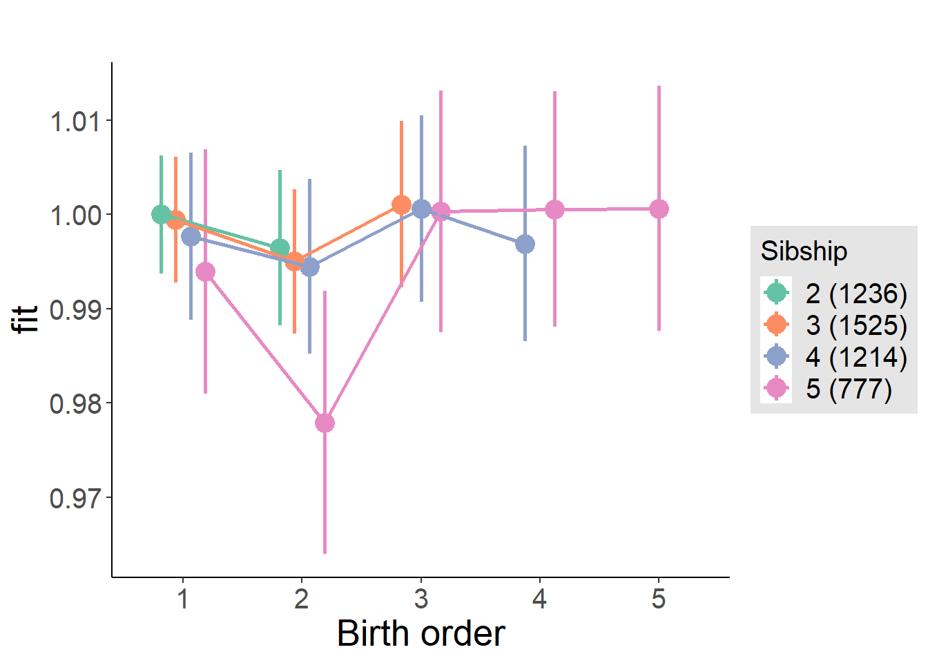
Model Comparison
###### Model 1 - Model 2
anova(m1_covariates_only, m2_birthorder_linear, m3_birthorder_nonlinear, m4_interaction)## refitting model(s) with ML (instead of REML)| Df | AIC | BIC | logLik | deviance | Chisq | Chi Df | Pr(>Chisq) |
|---|---|---|---|---|---|---|---|
| 10 | -13878 | -13813 | 6949 | -13898 | NA | NA | NA |
| 11 | -13878 | -13807 | 6950 | -13900 | 1.867 | 1 | 0.1719 |
| 14 | -13884 | -13794 | 6956 | -13912 | 12.78 | 3 | 0.005144 |
| 20 | -13881 | -13751 | 6960 | -13921 | 8.283 | 6 | 0.2181 |
Maternal pregnancy order
outcome_preg_m1 <- update(m2_birthorder_linear, data = birthorder %>%
mutate(sibling_count = sibling_count_uterus_preg_factor,
birth_order_nonlinear = birthorder_uterus_preg_factor,
birth_order = birthorder_uterus_preg,
count_birth_order = count_birthorder_uterus_preg
) %>%
filter(sibling_count != "1"))
compare_models_markdown(outcome_preg_m1)Basic Model
Model Summary
m1_covariates_only <- update(m2_birthorder_linear, formula = . ~ . - birth_order)
tidy(m1_covariates_only, conf.int = T, conf.level = 0.995)| effect | group | term | estimate | std.error | statistic | df | p.value | conf.low | conf.high |
|---|---|---|---|---|---|---|---|---|---|
| fixed | NA | (Intercept) | 0.9581 | 0.03124 | 30.67 | 4383 | 2.929e-187 | 0.8704 | 1.046 |
| fixed | NA | poly(age, 3, raw = TRUE)1 | 0.004337 | 0.003649 | 1.188 | 4362 | 0.2347 | -0.005906 | 0.01458 |
| fixed | NA | poly(age, 3, raw = TRUE)2 | -0.0001472 | 0.0001345 | -1.094 | 4336 | 0.2741 | -0.0005249 | 0.0002305 |
| fixed | NA | poly(age, 3, raw = TRUE)3 | 0.000001606 | 0.000001577 | 1.018 | 4309 | 0.3087 | -0.000002821 | 0.000006033 |
| fixed | NA | male | -0.001817 | 0.001698 | -1.071 | 4400 | 0.2844 | -0.006582 | 0.002948 |
| fixed | NA | sibling_count3 | -0.0002619 | 0.002345 | -0.1117 | 2586 | 0.9111 | -0.006843 | 0.006319 |
| fixed | NA | sibling_count4 | -0.00004756 | 0.002458 | -0.01935 | 2083 | 0.9846 | -0.006948 | 0.006853 |
| fixed | NA | sibling_count5 | -0.002108 | 0.002627 | -0.8025 | 1639 | 0.4224 | -0.009481 | 0.005265 |
| ran_pars | mother_pidlink | sd__(Intercept) | 0.001143 | NA | NA | NA | NA | NA | NA |
| ran_pars | Residual | sd__Observation | 0.05625 | NA | NA | NA | NA | NA | NA |
Coefficient Plot
plot(allEffects(m1_covariates_only, confidence.level = 0.995))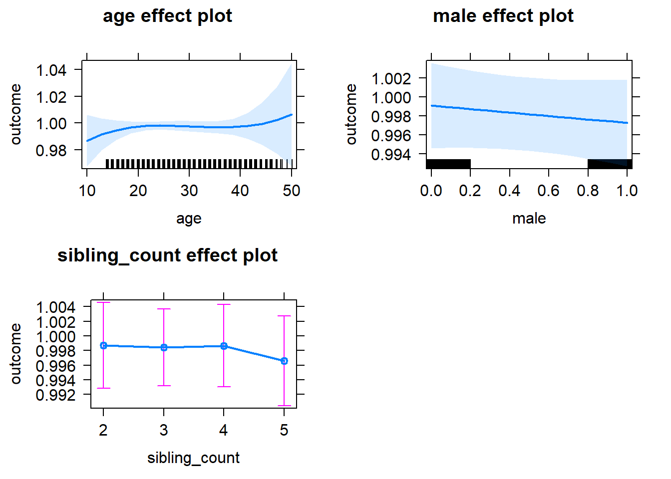
Add Birth Order Linear
Model Summary
tidy(m2_birthorder_linear, conf.int = T, conf.level = 0.995)| effect | group | term | estimate | std.error | statistic | df | p.value | conf.low | conf.high |
|---|---|---|---|---|---|---|---|---|---|
| fixed | NA | (Intercept) | 0.9565 | 0.03128 | 30.58 | 4381 | 2.553e-186 | 0.8687 | 1.044 |
| fixed | NA | birth_order | 0.0009232 | 0.000866 | 1.066 | 4120 | 0.2865 | -0.001508 | 0.003354 |
| fixed | NA | poly(age, 3, raw = TRUE)1 | 0.004395 | 0.003649 | 1.204 | 4360 | 0.2286 | -0.005849 | 0.01464 |
| fixed | NA | poly(age, 3, raw = TRUE)2 | -0.0001504 | 0.0001346 | -1.117 | 4335 | 0.2639 | -0.0005281 | 0.0002274 |
| fixed | NA | poly(age, 3, raw = TRUE)3 | 0.000001661 | 0.000001578 | 1.052 | 4309 | 0.2927 | -0.000002769 | 0.00000609 |
| fixed | NA | male | -0.001831 | 0.001698 | -1.078 | 4399 | 0.2809 | -0.006596 | 0.002935 |
| fixed | NA | sibling_count3 | -0.0006873 | 0.002378 | -0.289 | 2634 | 0.7726 | -0.007363 | 0.005989 |
| fixed | NA | sibling_count4 | -0.0009723 | 0.002607 | -0.373 | 2291 | 0.7092 | -0.00829 | 0.006345 |
| fixed | NA | sibling_count5 | -0.003582 | 0.002968 | -1.207 | 2095 | 0.2277 | -0.01191 | 0.00475 |
| ran_pars | mother_pidlink | sd__(Intercept) | 0.001379 | NA | NA | NA | NA | NA | NA |
| ran_pars | Residual | sd__Observation | 0.05625 | NA | NA | NA | NA | NA | NA |
Coefficient Plot
plot_birthorder2(m2_birthorder_linear, separate = FALSE)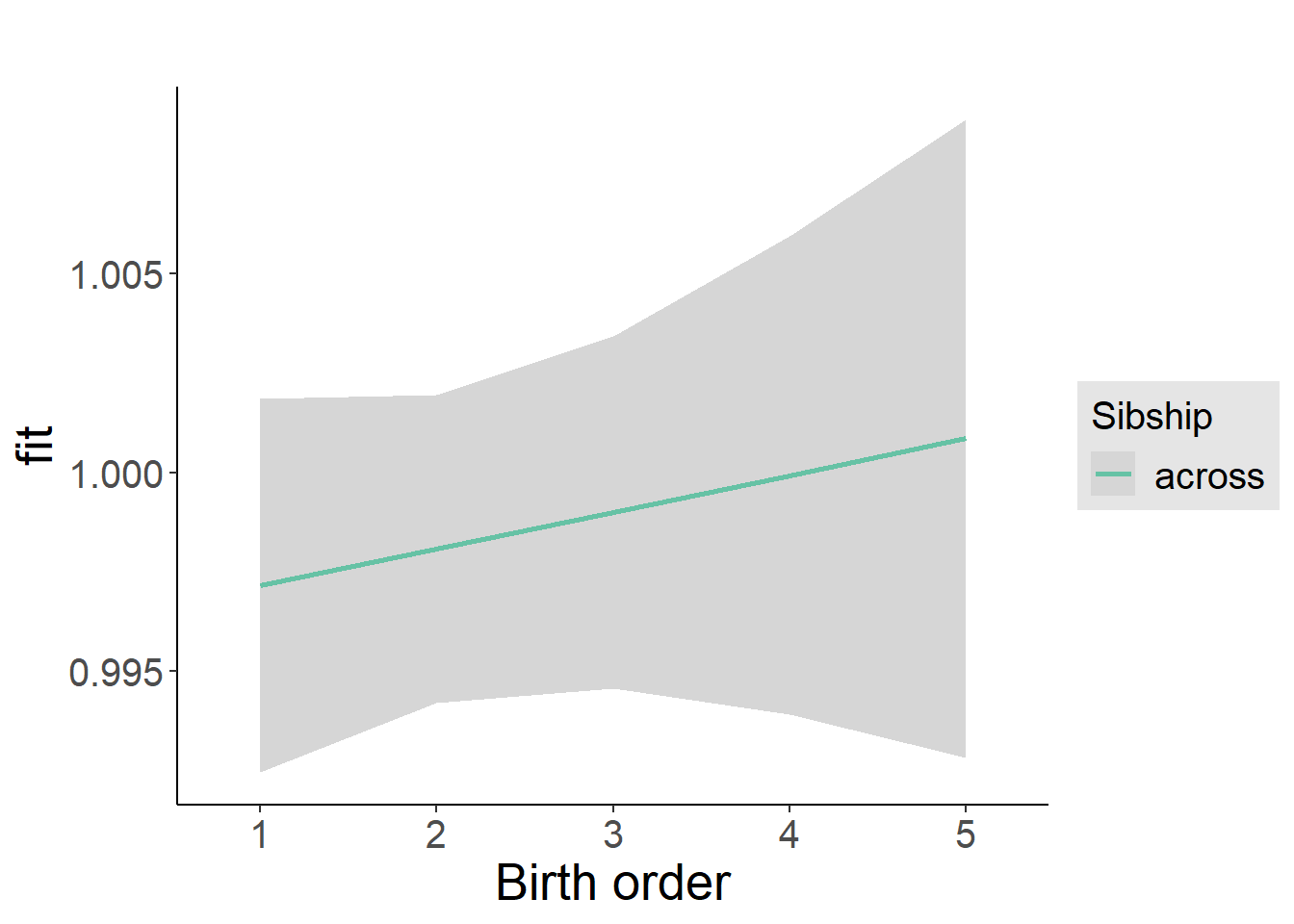
Add Birth Order Factor
Model Summary
m3_birthorder_nonlinear = update(m1_covariates_only, formula = . ~ . + birth_order_nonlinear)## boundary (singular) fit: see ?isSingulartidy(m3_birthorder_nonlinear, conf.int = T, conf.level = 0.995)| effect | group | term | estimate | std.error | statistic | df | p.value | conf.low | conf.high |
|---|---|---|---|---|---|---|---|---|---|
| fixed | NA | (Intercept) | 0.9612 | 0.03127 | 30.74 | 4400 | 3.926e-188 | 0.8734 | 1.049 |
| fixed | NA | poly(age, 3, raw = TRUE)1 | 0.004173 | 0.003649 | 1.144 | 4400 | 0.2528 | -0.00607 | 0.01442 |
| fixed | NA | poly(age, 3, raw = TRUE)2 | -0.0001422 | 0.0001346 | -1.057 | 4400 | 0.2908 | -0.0005199 | 0.0002356 |
| fixed | NA | poly(age, 3, raw = TRUE)3 | 0.000001568 | 0.000001578 | 0.9941 | 4400 | 0.3202 | -0.00000286 | 0.000005997 |
| fixed | NA | male | -0.001912 | 0.001697 | -1.127 | 4400 | 0.2597 | -0.006675 | 0.00285 |
| fixed | NA | sibling_count3 | -0.001068 | 0.002416 | -0.4419 | 4400 | 0.6586 | -0.007849 | 0.005714 |
| fixed | NA | sibling_count4 | -0.001268 | 0.002645 | -0.4793 | 4400 | 0.6318 | -0.008693 | 0.006158 |
| fixed | NA | sibling_count5 | -0.004737 | 0.002999 | -1.579 | 4400 | 0.1143 | -0.01316 | 0.003682 |
| fixed | NA | birth_order_nonlinear2 | -0.004602 | 0.002059 | -2.235 | 4400 | 0.02546 | -0.01038 | 0.001178 |
| fixed | NA | birth_order_nonlinear3 | 0.003053 | 0.002589 | 1.179 | 4400 | 0.2383 | -0.004214 | 0.01032 |
| fixed | NA | birth_order_nonlinear4 | 0.001132 | 0.003438 | 0.3293 | 4400 | 0.742 | -0.008518 | 0.01078 |
| fixed | NA | birth_order_nonlinear5 | 0.005537 | 0.005053 | 1.096 | 4400 | 0.2733 | -0.008648 | 0.01972 |
| ran_pars | mother_pidlink | sd__(Intercept) | 0 | NA | NA | NA | NA | NA | NA |
| ran_pars | Residual | sd__Observation | 0.05622 | NA | NA | NA | NA | NA | NA |
Coefficient Plot
plot_birthorder(m3_birthorder_nonlinear, separate = FALSE)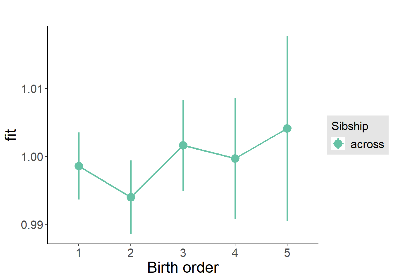
Add Interaction
Model Summary
m4_interaction = update(m3_birthorder_nonlinear, formula = . ~ . - birth_order_nonlinear - sibling_count + count_birth_order)## boundary (singular) fit: see ?isSingulartidy(m4_interaction, conf.int = T, conf.level = 0.995)| effect | group | term | estimate | std.error | statistic | df | p.value | conf.low | conf.high |
|---|---|---|---|---|---|---|---|---|---|
| fixed | NA | (Intercept) | 0.9607 | 0.03129 | 30.7 | 4394 | 1.067e-187 | 0.8729 | 1.049 |
| fixed | NA | poly(age, 3, raw = TRUE)1 | 0.004221 | 0.00365 | 1.156 | 4394 | 0.2476 | -0.006026 | 0.01447 |
| fixed | NA | poly(age, 3, raw = TRUE)2 | -0.0001441 | 0.0001346 | -1.071 | 4394 | 0.2844 | -0.0005221 | 0.0002338 |
| fixed | NA | poly(age, 3, raw = TRUE)3 | 0.000001594 | 0.000001579 | 1.01 | 4394 | 0.3126 | -0.000002837 | 0.000006026 |
| fixed | NA | male | -0.001903 | 0.001698 | -1.121 | 4394 | 0.2623 | -0.006668 | 0.002862 |
| fixed | NA | count_birth_order2/2 | -0.004156 | 0.003696 | -1.124 | 4394 | 0.261 | -0.01453 | 0.00622 |
| fixed | NA | count_birth_order1/3 | -0.0004909 | 0.003182 | -0.1543 | 4394 | 0.8774 | -0.009424 | 0.008442 |
| fixed | NA | count_birth_order2/3 | -0.005566 | 0.003461 | -1.608 | 4394 | 0.1078 | -0.01528 | 0.004148 |
| fixed | NA | count_birth_order3/3 | 0.001399 | 0.003874 | 0.3611 | 4394 | 0.718 | -0.009476 | 0.01227 |
| fixed | NA | count_birth_order1/4 | -0.001895 | 0.003754 | -0.5047 | 4394 | 0.6138 | -0.01243 | 0.008643 |
| fixed | NA | count_birth_order2/4 | -0.00205 | 0.003829 | -0.5353 | 4394 | 0.5925 | -0.0128 | 0.008698 |
| fixed | NA | count_birth_order3/4 | 0.001059 | 0.004206 | 0.2517 | 4394 | 0.8013 | -0.01075 | 0.01287 |
| fixed | NA | count_birth_order4/4 | -0.00314 | 0.004349 | -0.722 | 4394 | 0.4703 | -0.01535 | 0.009067 |
| fixed | NA | count_birth_order1/5 | -0.004016 | 0.004481 | -0.8961 | 4394 | 0.3702 | -0.0166 | 0.008563 |
| fixed | NA | count_birth_order2/5 | -0.01644 | 0.004817 | -3.413 | 4394 | 0.0006489 | -0.02996 | -0.002918 |
| fixed | NA | count_birth_order3/5 | 0.0008529 | 0.004687 | 0.182 | 4394 | 0.8556 | -0.0123 | 0.01401 |
| fixed | NA | count_birth_order4/5 | 0.0008388 | 0.004914 | 0.1707 | 4394 | 0.8645 | -0.01295 | 0.01463 |
| fixed | NA | count_birth_order5/5 | 0.0009558 | 0.004891 | 0.1954 | 4394 | 0.8451 | -0.01277 | 0.01468 |
| ran_pars | mother_pidlink | sd__(Intercept) | 0 | NA | NA | NA | NA | NA | NA |
| ran_pars | Residual | sd__Observation | 0.05621 | NA | NA | NA | NA | NA | NA |
Coefficient Plot
plot_birthorder(m4_interaction)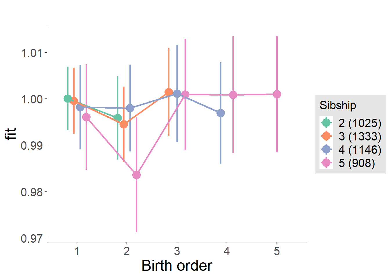
Model Comparison
###### Model 1 - Model 2
anova(m1_covariates_only, m2_birthorder_linear, m3_birthorder_nonlinear, m4_interaction)## refitting model(s) with ML (instead of REML)| Df | AIC | BIC | logLik | deviance | Chisq | Chi Df | Pr(>Chisq) |
|---|---|---|---|---|---|---|---|
| 10 | -12860 | -12796 | 6440 | -12880 | NA | NA | NA |
| 11 | -12859 | -12789 | 6441 | -12881 | 1.138 | 1 | 0.286 |
| 14 | -12863 | -12774 | 6446 | -12891 | 10.02 | 3 | 0.01836 |
| 20 | -12858 | -12730 | 6449 | -12898 | 6.595 | 6 | 0.3599 |
Parental full sibling order
outcome_parental_m1 <- update(m2_birthorder_linear, data = birthorder %>%
mutate(sibling_count = sibling_count_genes_factor,
birth_order_nonlinear = birthorder_genes_factor,
birth_order = birthorder_genes,
count_birth_order = count_birthorder_genes
) %>%
filter(sibling_count != "1"))## boundary (singular) fit: see ?isSingularcompare_models_markdown(outcome_parental_m1)Basic Model
Model Summary
m1_covariates_only <- update(m2_birthorder_linear, formula = . ~ . - birth_order)## boundary (singular) fit: see ?isSingulartidy(m1_covariates_only, conf.int = T, conf.level = 0.995)| effect | group | term | estimate | std.error | statistic | df | p.value | conf.low | conf.high |
|---|---|---|---|---|---|---|---|---|---|
| fixed | NA | (Intercept) | 0.9834 | 0.03057 | 32.17 | 4729 | 1.848e-205 | 0.8976 | 1.069 |
| fixed | NA | poly(age, 3, raw = TRUE)1 | 0.001608 | 0.003572 | 0.4502 | 4729 | 0.6526 | -0.008418 | 0.01163 |
| fixed | NA | poly(age, 3, raw = TRUE)2 | -0.00005133 | 0.0001318 | -0.3895 | 4729 | 0.6969 | -0.0004213 | 0.0003186 |
| fixed | NA | poly(age, 3, raw = TRUE)3 | 0.0000005632 | 0.000001547 | 0.364 | 4729 | 0.7159 | -0.000003781 | 0.000004907 |
| fixed | NA | male | -0.002083 | 0.001636 | -1.274 | 4729 | 0.2028 | -0.006675 | 0.002508 |
| fixed | NA | sibling_count3 | -0.001204 | 0.002128 | -0.5657 | 4729 | 0.5716 | -0.007178 | 0.00477 |
| fixed | NA | sibling_count4 | -0.003955 | 0.002293 | -1.725 | 4729 | 0.08459 | -0.01039 | 0.002481 |
| fixed | NA | sibling_count5 | -0.003413 | 0.002687 | -1.27 | 4729 | 0.2041 | -0.01096 | 0.00413 |
| ran_pars | mother_pidlink | sd__(Intercept) | 0.000000007554 | NA | NA | NA | NA | NA | NA |
| ran_pars | Residual | sd__Observation | 0.05619 | NA | NA | NA | NA | NA | NA |
Coefficient Plot
plot(allEffects(m1_covariates_only, confidence.level = 0.995))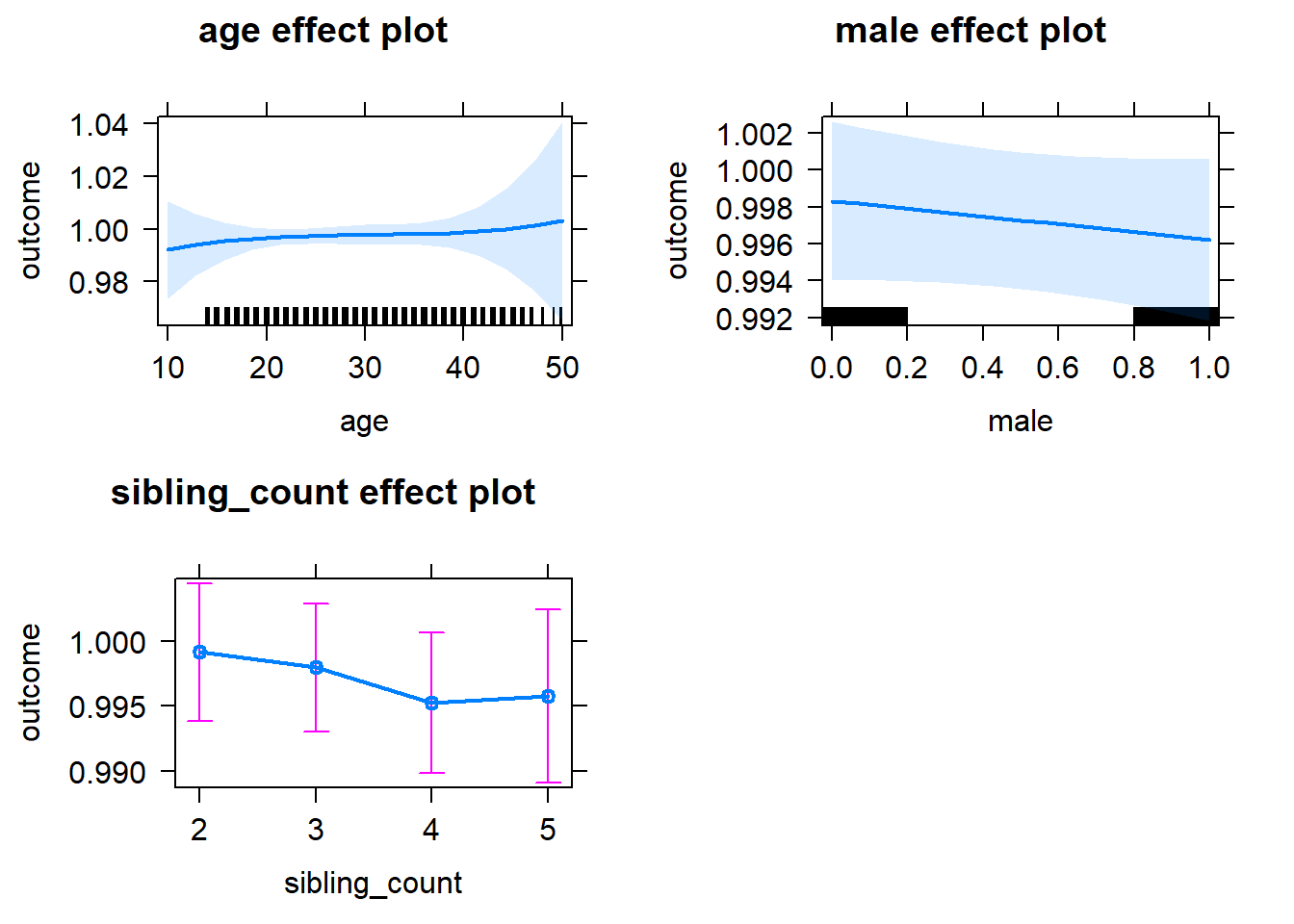
Add Birth Order Linear
Model Summary
tidy(m2_birthorder_linear, conf.int = T, conf.level = 0.995)| effect | group | term | estimate | std.error | statistic | df | p.value | conf.low | conf.high |
|---|---|---|---|---|---|---|---|---|---|
| fixed | NA | (Intercept) | 0.9825 | 0.03061 | 32.1 | 4728 | 1.192e-204 | 0.8966 | 1.068 |
| fixed | NA | birth_order | 0.0005388 | 0.0008783 | 0.6135 | 4728 | 0.5396 | -0.001927 | 0.003004 |
| fixed | NA | poly(age, 3, raw = TRUE)1 | 0.001642 | 0.003572 | 0.4596 | 4728 | 0.6458 | -0.008386 | 0.01167 |
| fixed | NA | poly(age, 3, raw = TRUE)2 | -0.00005322 | 0.0001318 | -0.4037 | 4728 | 0.6865 | -0.0004233 | 0.0003169 |
| fixed | NA | poly(age, 3, raw = TRUE)3 | 0.0000005956 | 0.000001548 | 0.3847 | 4728 | 0.7005 | -0.000003751 | 0.000004942 |
| fixed | NA | male | -0.002095 | 0.001636 | -1.281 | 4728 | 0.2003 | -0.006687 | 0.002496 |
| fixed | NA | sibling_count3 | -0.001451 | 0.002166 | -0.6699 | 4728 | 0.5029 | -0.007532 | 0.00463 |
| fixed | NA | sibling_count4 | -0.004511 | 0.002465 | -1.83 | 4728 | 0.06737 | -0.01143 | 0.00241 |
| fixed | NA | sibling_count5 | -0.004303 | 0.003054 | -1.409 | 4728 | 0.1589 | -0.01288 | 0.00427 |
| ran_pars | mother_pidlink | sd__(Intercept) | 0.000000002149 | NA | NA | NA | NA | NA | NA |
| ran_pars | Residual | sd__Observation | 0.0562 | NA | NA | NA | NA | NA | NA |
Coefficient Plot
plot_birthorder2(m2_birthorder_linear, separate = FALSE)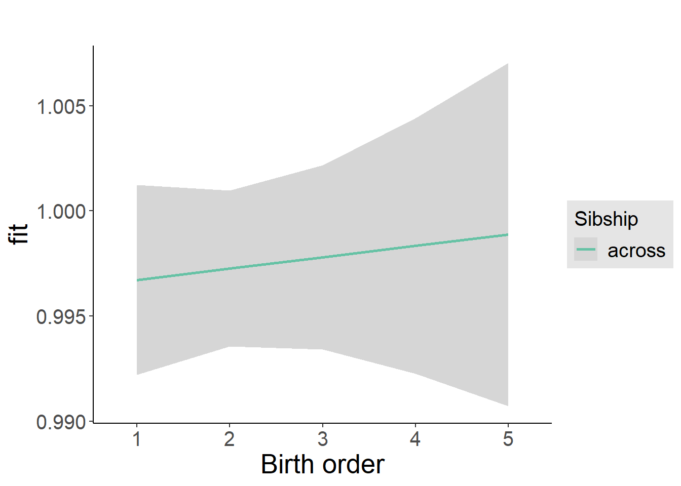
Add Birth Order Factor
Model Summary
m3_birthorder_nonlinear = update(m1_covariates_only, formula = . ~ . + birth_order_nonlinear)## boundary (singular) fit: see ?isSingulartidy(m3_birthorder_nonlinear, conf.int = T, conf.level = 0.995)| effect | group | term | estimate | std.error | statistic | df | p.value | conf.low | conf.high |
|---|---|---|---|---|---|---|---|---|---|
| fixed | NA | (Intercept) | 0.9856 | 0.03061 | 32.2 | 4725 | 7.279e-206 | 0.8996 | 1.071 |
| fixed | NA | poly(age, 3, raw = TRUE)1 | 0.001544 | 0.003572 | 0.4323 | 4725 | 0.6656 | -0.008483 | 0.01157 |
| fixed | NA | poly(age, 3, raw = TRUE)2 | -0.00004998 | 0.0001318 | -0.3791 | 4725 | 0.7046 | -0.0004201 | 0.0003201 |
| fixed | NA | poly(age, 3, raw = TRUE)3 | 0.0000005631 | 0.000001548 | 0.3637 | 4725 | 0.7161 | -0.000003783 | 0.000004909 |
| fixed | NA | male | -0.002095 | 0.001635 | -1.281 | 4725 | 0.2001 | -0.006684 | 0.002494 |
| fixed | NA | sibling_count3 | -0.002215 | 0.002205 | -1.004 | 4725 | 0.3152 | -0.008405 | 0.003975 |
| fixed | NA | sibling_count4 | -0.005696 | 0.002506 | -2.273 | 4725 | 0.02307 | -0.01273 | 0.001338 |
| fixed | NA | sibling_count5 | -0.004886 | 0.003121 | -1.566 | 4725 | 0.1175 | -0.01365 | 0.003873 |
| fixed | NA | birth_order_nonlinear2 | -0.004122 | 0.001966 | -2.097 | 4725 | 0.03609 | -0.009641 | 0.001397 |
| fixed | NA | birth_order_nonlinear3 | 0.003645 | 0.002506 | 1.455 | 4725 | 0.1458 | -0.003388 | 0.01068 |
| fixed | NA | birth_order_nonlinear4 | 0.002612 | 0.003452 | 0.7568 | 4725 | 0.4492 | -0.007076 | 0.0123 |
| fixed | NA | birth_order_nonlinear5 | -0.003081 | 0.005663 | -0.5441 | 4725 | 0.5864 | -0.01898 | 0.01281 |
| ran_pars | mother_pidlink | sd__(Intercept) | 0.000000002736 | NA | NA | NA | NA | NA | NA |
| ran_pars | Residual | sd__Observation | 0.05615 | NA | NA | NA | NA | NA | NA |
Coefficient Plot
plot_birthorder(m3_birthorder_nonlinear, separate = FALSE)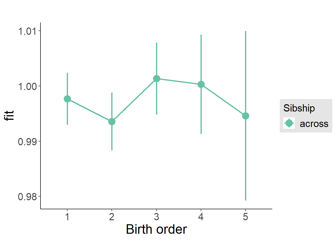
Add Interaction
Model Summary
m4_interaction = update(m3_birthorder_nonlinear, formula = . ~ . - birth_order_nonlinear - sibling_count + count_birth_order)## boundary (singular) fit: see ?isSingulartidy(m4_interaction, conf.int = T, conf.level = 0.995)| effect | group | term | estimate | std.error | statistic | df | p.value | conf.low | conf.high |
|---|---|---|---|---|---|---|---|---|---|
| fixed | NA | (Intercept) | 0.9865 | 0.03062 | 32.22 | 4719 | 4.308e-206 | 0.9006 | 1.072 |
| fixed | NA | poly(age, 3, raw = TRUE)1 | 0.00144 | 0.003573 | 0.4028 | 4719 | 0.6871 | -0.008591 | 0.01147 |
| fixed | NA | poly(age, 3, raw = TRUE)2 | -0.00004624 | 0.0001319 | -0.3506 | 4719 | 0.7259 | -0.0004165 | 0.000324 |
| fixed | NA | poly(age, 3, raw = TRUE)3 | 0.0000005237 | 0.000001549 | 0.3381 | 4719 | 0.7353 | -0.000003824 | 0.000004872 |
| fixed | NA | male | -0.002104 | 0.001635 | -1.287 | 4719 | 0.1983 | -0.006695 | 0.002487 |
| fixed | NA | count_birth_order2/2 | -0.004447 | 0.003281 | -1.356 | 4719 | 0.1753 | -0.01366 | 0.004762 |
| fixed | NA | count_birth_order1/3 | -0.001683 | 0.002898 | -0.5809 | 4719 | 0.5613 | -0.009817 | 0.006451 |
| fixed | NA | count_birth_order2/3 | -0.006297 | 0.003198 | -1.969 | 4719 | 0.04904 | -0.01527 | 0.002681 |
| fixed | NA | count_birth_order3/3 | -0.0001277 | 0.003518 | -0.03631 | 4719 | 0.971 | -0.01 | 0.009746 |
| fixed | NA | count_birth_order1/4 | -0.009212 | 0.003603 | -2.557 | 4719 | 0.0106 | -0.01933 | 0.0009016 |
| fixed | NA | count_birth_order2/4 | -0.006819 | 0.003717 | -1.835 | 4719 | 0.06662 | -0.01725 | 0.003614 |
| fixed | NA | count_birth_order3/4 | -0.0005325 | 0.003895 | -0.1367 | 4719 | 0.8913 | -0.01147 | 0.0104 |
| fixed | NA | count_birth_order4/4 | -0.004344 | 0.004113 | -1.056 | 4719 | 0.2909 | -0.01589 | 0.007201 |
| fixed | NA | count_birth_order1/5 | -0.00103 | 0.0049 | -0.2101 | 4719 | 0.8336 | -0.01479 | 0.01273 |
| fixed | NA | count_birth_order2/5 | -0.01707 | 0.005439 | -3.139 | 4719 | 0.001708 | -0.03234 | -0.001804 |
| fixed | NA | count_birth_order3/5 | -0.000926 | 0.005104 | -0.1814 | 4719 | 0.856 | -0.01525 | 0.0134 |
| fixed | NA | count_birth_order4/5 | -0.0005586 | 0.005017 | -0.1114 | 4719 | 0.9113 | -0.01464 | 0.01352 |
| fixed | NA | count_birth_order5/5 | -0.008091 | 0.005307 | -1.524 | 4719 | 0.1275 | -0.02299 | 0.006807 |
| ran_pars | mother_pidlink | sd__(Intercept) | 0.000000006019 | NA | NA | NA | NA | NA | NA |
| ran_pars | Residual | sd__Observation | 0.05615 | NA | NA | NA | NA | NA | NA |
Coefficient Plot
plot_birthorder(m4_interaction)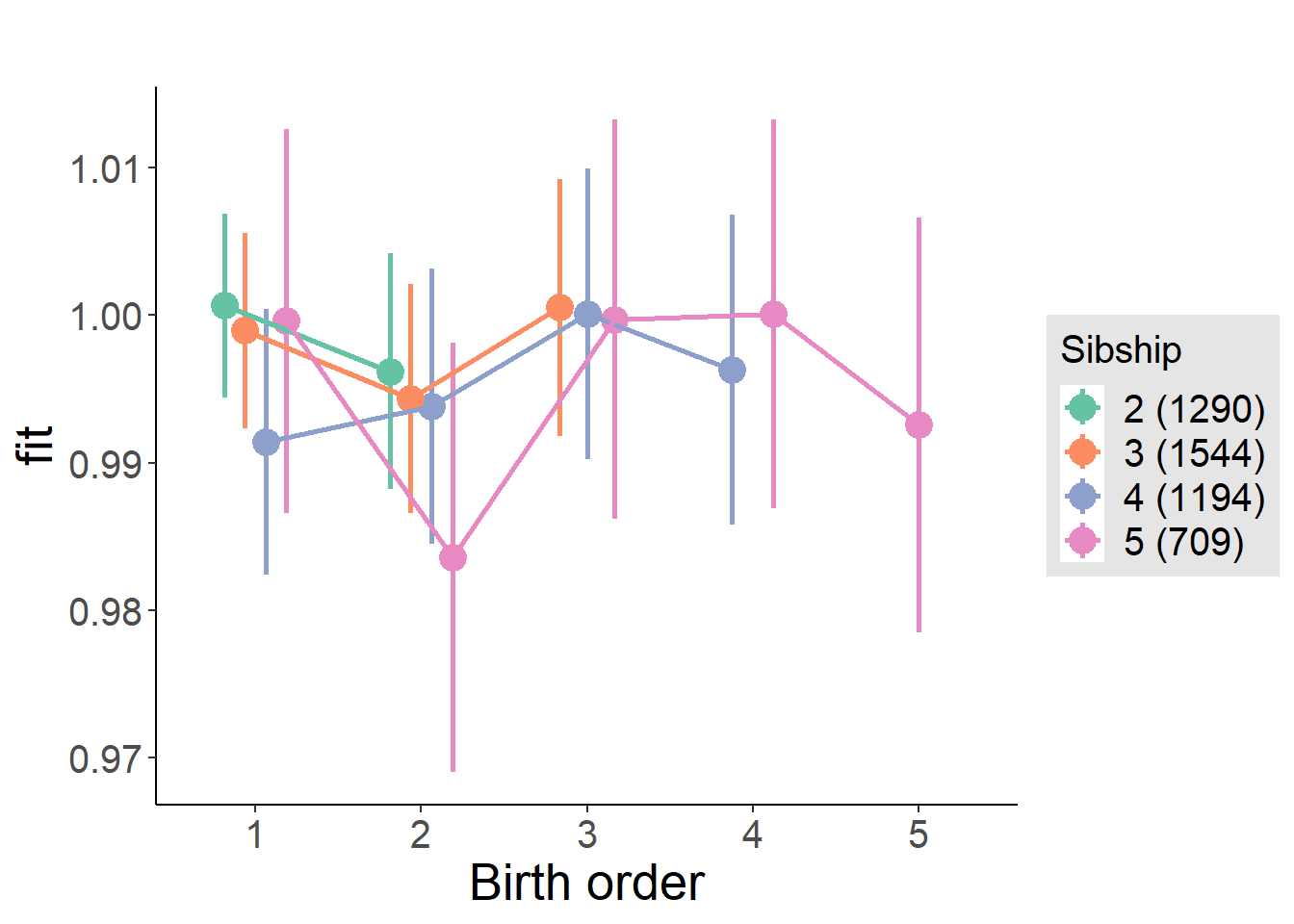
Model Comparison
###### Model 1 - Model 2
anova(m1_covariates_only, m2_birthorder_linear, m3_birthorder_nonlinear, m4_interaction)## refitting model(s) with ML (instead of REML)| Df | AIC | BIC | logLik | deviance | Chisq | Chi Df | Pr(>Chisq) |
|---|---|---|---|---|---|---|---|
| 10 | -13820 | -13756 | 6920 | -13840 | NA | NA | NA |
| 11 | -13819 | -13748 | 6920 | -13841 | 0.377 | 1 | 0.5392 |
| 14 | -13823 | -13733 | 6926 | -13851 | 10.69 | 3 | 0.01354 |
| 20 | -13818 | -13689 | 6929 | -13858 | 6.457 | 6 | 0.3739 |
Compare birth order specifications
library(coefplot)
multiplot(outcome_naive_m1, outcome_preg_m1, outcome_uterus_m1, outcome_parental_m1, dodgeHeight = 0.6,
intercept = FALSE)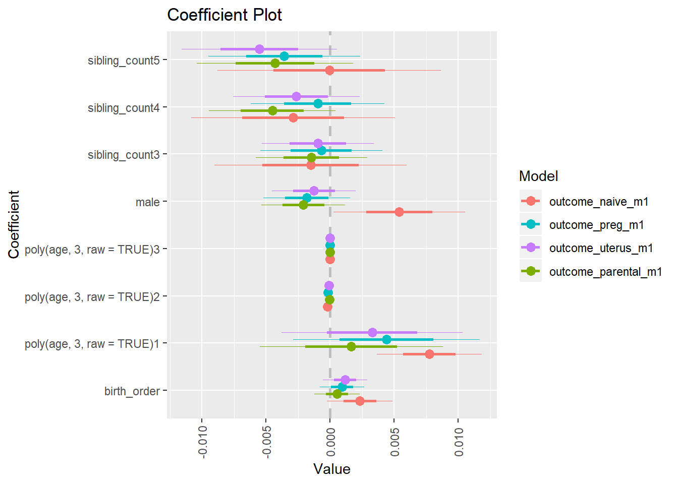
Work
Income Last Month (log) - z-standardized
birthorder <- birthorder %>% mutate(outcome = wage_last_month_z)
model = lmer(outcome ~ birth_order + poly(age, 3, raw = TRUE) + male + sibling_count + (1 | mother_pidlink),
data = birthorder)
compare_birthorder_specs(model)Naive birth order
outcome_naive_m1 <- update(m2_birthorder_linear, data = birthorder %>%
mutate(sibling_count = sibling_count_naive_factor,
birth_order_nonlinear = birthorder_naive_factor,
birth_order = birthorder_naive,
count_birth_order = count_birthorder_naive) %>%
filter(sibling_count != "1"))
compare_models_markdown(outcome_naive_m1)Basic Model
Model Summary
m1_covariates_only <- update(m2_birthorder_linear, formula = . ~ . - birth_order)
tidy(m1_covariates_only, conf.int = T, conf.level = 0.995)| effect | group | term | estimate | std.error | statistic | df | p.value | conf.low | conf.high |
|---|---|---|---|---|---|---|---|---|---|
| fixed | NA | (Intercept) | -2.49 | 0.4698 | -5.301 | 2910 | 0.0000001237 | -3.809 | -1.172 |
| fixed | NA | poly(age, 3, raw = TRUE)1 | 0.1928 | 0.04401 | 4.381 | 2904 | 0.00001223 | 0.06928 | 0.3164 |
| fixed | NA | poly(age, 3, raw = TRUE)2 | -0.004761 | 0.001292 | -3.686 | 2903 | 0.0002323 | -0.008387 | -0.001135 |
| fixed | NA | poly(age, 3, raw = TRUE)3 | 0.00003689 | 0.00001197 | 3.081 | 2909 | 0.002084 | 0.000003278 | 0.00007049 |
| fixed | NA | male | 0.1129 | 0.03649 | 3.095 | 2919 | 0.001988 | 0.0105 | 0.2153 |
| fixed | NA | sibling_count3 | 0.102 | 0.0525 | 1.944 | 2122 | 0.05207 | -0.04533 | 0.2494 |
| fixed | NA | sibling_count4 | 0.05001 | 0.05263 | 0.9503 | 2019 | 0.3421 | -0.09771 | 0.1977 |
| fixed | NA | sibling_count5 | 0.04399 | 0.05502 | 0.7995 | 1914 | 0.4241 | -0.1104 | 0.1984 |
| ran_pars | mother_pidlink | sd__(Intercept) | 0.423 | NA | NA | NA | NA | NA | NA |
| ran_pars | Residual | sd__Observation | 0.8809 | NA | NA | NA | NA | NA | NA |
Coefficient Plot
plot(allEffects(m1_covariates_only, confidence.level = 0.995))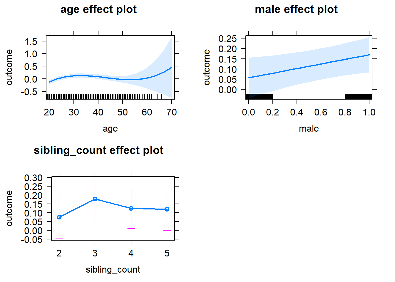
Add Birth Order Linear
Model Summary
tidy(m2_birthorder_linear, conf.int = T, conf.level = 0.995)| effect | group | term | estimate | std.error | statistic | df | p.value | conf.low | conf.high |
|---|---|---|---|---|---|---|---|---|---|
| fixed | NA | (Intercept) | -2.491 | 0.4698 | -5.303 | 2909 | 0.0000001228 | -3.81 | -1.172 |
| fixed | NA | birth_order | 0.01003 | 0.01754 | 0.5719 | 2449 | 0.5674 | -0.03921 | 0.05927 |
| fixed | NA | poly(age, 3, raw = TRUE)1 | 0.1918 | 0.04406 | 4.352 | 2904 | 0.00001393 | 0.06808 | 0.3154 |
| fixed | NA | poly(age, 3, raw = TRUE)2 | -0.004738 | 0.001293 | -3.666 | 2902 | 0.0002513 | -0.008366 | -0.00111 |
| fixed | NA | poly(age, 3, raw = TRUE)3 | 0.00003678 | 0.00001198 | 3.071 | 2908 | 0.002153 | 0.000003162 | 0.0000704 |
| fixed | NA | male | 0.113 | 0.03649 | 3.098 | 2917 | 0.00197 | 0.0106 | 0.2155 |
| fixed | NA | sibling_count3 | 0.09832 | 0.05291 | 1.858 | 2174 | 0.06325 | -0.05019 | 0.2468 |
| fixed | NA | sibling_count4 | 0.04142 | 0.05474 | 0.7567 | 2247 | 0.4493 | -0.1122 | 0.1951 |
| fixed | NA | sibling_count5 | 0.03035 | 0.05997 | 0.5061 | 2363 | 0.6129 | -0.138 | 0.1987 |
| ran_pars | mother_pidlink | sd__(Intercept) | 0.4235 | NA | NA | NA | NA | NA | NA |
| ran_pars | Residual | sd__Observation | 0.8808 | NA | NA | NA | NA | NA | NA |
Coefficient Plot
plot_birthorder2(m2_birthorder_linear, separate = FALSE)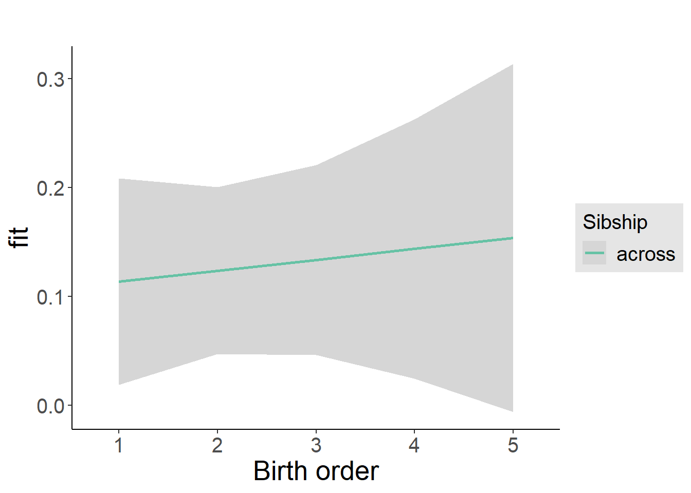
Add Birth Order Factor
Model Summary
m3_birthorder_nonlinear = update(m1_covariates_only, formula = . ~ . + birth_order_nonlinear)
tidy(m3_birthorder_nonlinear, conf.int = T, conf.level = 0.995)| effect | group | term | estimate | std.error | statistic | df | p.value | conf.low | conf.high |
|---|---|---|---|---|---|---|---|---|---|
| fixed | NA | (Intercept) | -2.475 | 0.471 | -5.254 | 2904 | 0.0000001594 | -3.797 | -1.153 |
| fixed | NA | poly(age, 3, raw = TRUE)1 | 0.1908 | 0.04412 | 4.324 | 2896 | 0.00001584 | 0.06693 | 0.3146 |
| fixed | NA | poly(age, 3, raw = TRUE)2 | -0.004707 | 0.001295 | -3.634 | 2891 | 0.0002841 | -0.008343 | -0.001071 |
| fixed | NA | poly(age, 3, raw = TRUE)3 | 0.00003648 | 0.00001201 | 3.037 | 2895 | 0.002412 | 0.00000276 | 0.00007019 |
| fixed | NA | male | 0.1122 | 0.03653 | 3.071 | 2916 | 0.002153 | 0.009647 | 0.2148 |
| fixed | NA | sibling_count3 | 0.108 | 0.05366 | 2.013 | 2255 | 0.04424 | -0.04261 | 0.2586 |
| fixed | NA | sibling_count4 | 0.05079 | 0.05561 | 0.9132 | 2337 | 0.3612 | -0.1053 | 0.2069 |
| fixed | NA | sibling_count5 | 0.03047 | 0.06048 | 0.5038 | 2412 | 0.6144 | -0.1393 | 0.2002 |
| fixed | NA | birth_order_nonlinear2 | 0.02079 | 0.04306 | 0.4827 | 2381 | 0.6293 | -0.1001 | 0.1417 |
| fixed | NA | birth_order_nonlinear3 | -0.02247 | 0.05386 | -0.4172 | 2315 | 0.6766 | -0.1737 | 0.1287 |
| fixed | NA | birth_order_nonlinear4 | 0.03629 | 0.06916 | 0.5247 | 2276 | 0.5998 | -0.1579 | 0.2304 |
| fixed | NA | birth_order_nonlinear5 | 0.09002 | 0.101 | 0.8911 | 2291 | 0.373 | -0.1935 | 0.3736 |
| ran_pars | mother_pidlink | sd__(Intercept) | 0.4231 | NA | NA | NA | NA | NA | NA |
| ran_pars | Residual | sd__Observation | 0.8812 | NA | NA | NA | NA | NA | NA |
Coefficient Plot
plot_birthorder(m3_birthorder_nonlinear, separate = FALSE)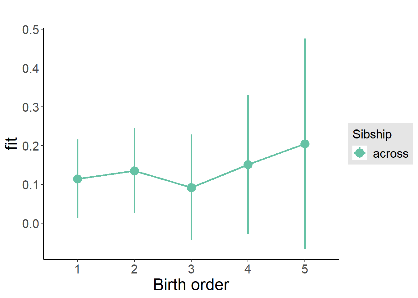
Add Interaction
Model Summary
m4_interaction = update(m3_birthorder_nonlinear, formula = . ~ . - birth_order_nonlinear - sibling_count + count_birth_order)
tidy(m4_interaction, conf.int = T, conf.level = 0.995)| effect | group | term | estimate | std.error | statistic | df | p.value | conf.low | conf.high |
|---|---|---|---|---|---|---|---|---|---|
| fixed | NA | (Intercept) | -2.445 | 0.4721 | -5.178 | 2903 | 0.0000002401 | -3.77 | -1.119 |
| fixed | NA | poly(age, 3, raw = TRUE)1 | 0.1889 | 0.0442 | 4.274 | 2892 | 0.00001982 | 0.06484 | 0.313 |
| fixed | NA | poly(age, 3, raw = TRUE)2 | -0.004649 | 0.001297 | -3.583 | 2887 | 0.0003452 | -0.00829 | -0.001007 |
| fixed | NA | poly(age, 3, raw = TRUE)3 | 0.00003591 | 0.00001203 | 2.986 | 2890 | 0.002855 | 0.000002147 | 0.00006968 |
| fixed | NA | male | 0.1122 | 0.03656 | 3.069 | 2907 | 0.002169 | 0.009572 | 0.2148 |
| fixed | NA | count_birth_order2/2 | -0.01542 | 0.07519 | -0.205 | 2478 | 0.8376 | -0.2265 | 0.1956 |
| fixed | NA | count_birth_order1/3 | 0.09647 | 0.06855 | 1.407 | 2940 | 0.1595 | -0.09596 | 0.2889 |
| fixed | NA | count_birth_order2/3 | 0.0873 | 0.07801 | 1.119 | 2944 | 0.2632 | -0.1317 | 0.3063 |
| fixed | NA | count_birth_order3/3 | 0.1128 | 0.08734 | 1.292 | 2917 | 0.1965 | -0.1323 | 0.358 |
| fixed | NA | count_birth_order1/4 | 0.05905 | 0.07606 | 0.7764 | 2947 | 0.4376 | -0.1545 | 0.2726 |
| fixed | NA | count_birth_order2/4 | 0.08377 | 0.0814 | 1.029 | 2942 | 0.3035 | -0.1447 | 0.3123 |
| fixed | NA | count_birth_order3/4 | -0.06199 | 0.08534 | -0.7265 | 2929 | 0.4676 | -0.3015 | 0.1775 |
| fixed | NA | count_birth_order4/4 | 0.1005 | 0.09323 | 1.078 | 2909 | 0.281 | -0.1612 | 0.3622 |
| fixed | NA | count_birth_order1/5 | -0.04536 | 0.08595 | -0.5278 | 2941 | 0.5977 | -0.2866 | 0.1959 |
| fixed | NA | count_birth_order2/5 | 0.09444 | 0.09483 | 0.9959 | 2896 | 0.3194 | -0.1718 | 0.3606 |
| fixed | NA | count_birth_order3/5 | 0.05258 | 0.09639 | 0.5455 | 2896 | 0.5855 | -0.218 | 0.3231 |
| fixed | NA | count_birth_order4/5 | 0.02558 | 0.0982 | 0.2605 | 2864 | 0.7945 | -0.2501 | 0.3012 |
| fixed | NA | count_birth_order5/5 | 0.1098 | 0.1016 | 1.081 | 2876 | 0.2798 | -0.1754 | 0.3951 |
| ran_pars | mother_pidlink | sd__(Intercept) | 0.4273 | NA | NA | NA | NA | NA | NA |
| ran_pars | Residual | sd__Observation | 0.8798 | NA | NA | NA | NA | NA | NA |
Coefficient Plot
plot_birthorder(m4_interaction)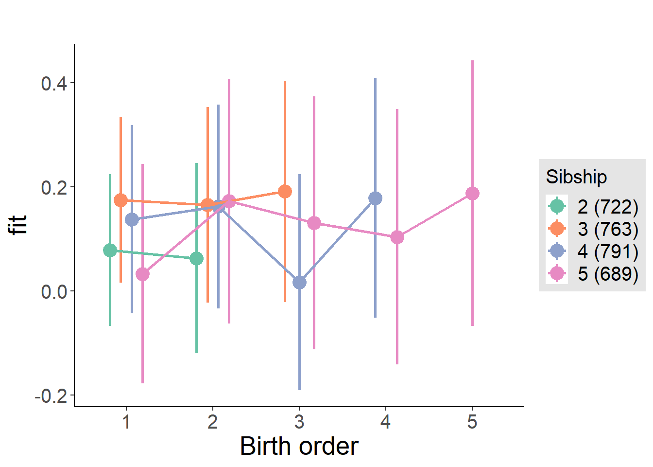
Model Comparison
###### Model 1 - Model 2
anova(m1_covariates_only, m2_birthorder_linear, m3_birthorder_nonlinear, m4_interaction)## refitting model(s) with ML (instead of REML)| Df | AIC | BIC | logLik | deviance | Chisq | Chi Df | Pr(>Chisq) |
|---|---|---|---|---|---|---|---|
| 10 | 8262 | 8322 | -4121 | 8242 | NA | NA | NA |
| 11 | 8264 | 8330 | -4121 | 8242 | 0.3266 | 1 | 0.5677 |
| 14 | 8269 | 8352 | -4120 | 8241 | 1.343 | 3 | 0.719 |
| 20 | 8276 | 8396 | -4118 | 8236 | 4.248 | 6 | 0.6431 |
Maternal birth order
outcome_uterus_m1 <- update(m2_birthorder_linear, data = birthorder %>%
mutate(sibling_count = sibling_count_uterus_alive_factor,
birth_order_nonlinear = birthorder_uterus_alive_factor,
birth_order = birthorder_uterus_alive,
count_birth_order = count_birthorder_uterus_alive) %>%
filter(sibling_count != "1"))
compare_models_markdown(outcome_uterus_m1)Basic Model
Model Summary
m1_covariates_only <- update(m2_birthorder_linear, formula = . ~ . - birth_order)
tidy(m1_covariates_only, conf.int = T, conf.level = 0.995)| effect | group | term | estimate | std.error | statistic | df | p.value | conf.low | conf.high |
|---|---|---|---|---|---|---|---|---|---|
| fixed | NA | (Intercept) | -2.234 | 1.071 | -2.087 | 1878 | 0.03701 | -5.239 | 0.7706 |
| fixed | NA | poly(age, 3, raw = TRUE)1 | 0.1599 | 0.1171 | 1.366 | 1879 | 0.172 | -0.1686 | 0.4885 |
| fixed | NA | poly(age, 3, raw = TRUE)2 | -0.003356 | 0.004111 | -0.8162 | 1880 | 0.4145 | -0.0149 | 0.008185 |
| fixed | NA | poly(age, 3, raw = TRUE)3 | 0.00002172 | 0.00004642 | 0.4679 | 1880 | 0.6399 | -0.0001086 | 0.000152 |
| fixed | NA | male | 0.1531 | 0.04496 | 3.405 | 1894 | 0.0006757 | 0.02688 | 0.2793 |
| fixed | NA | sibling_count3 | 0.05291 | 0.06084 | 0.8696 | 1517 | 0.3847 | -0.1179 | 0.2237 |
| fixed | NA | sibling_count4 | -0.06268 | 0.06288 | -0.9967 | 1404 | 0.3191 | -0.2392 | 0.1138 |
| fixed | NA | sibling_count5 | -0.1297 | 0.07171 | -1.809 | 1294 | 0.07062 | -0.331 | 0.07154 |
| ran_pars | mother_pidlink | sd__(Intercept) | 0.2516 | NA | NA | NA | NA | NA | NA |
| ran_pars | Residual | sd__Observation | 0.9272 | NA | NA | NA | NA | NA | NA |
Coefficient Plot
plot(allEffects(m1_covariates_only, confidence.level = 0.995))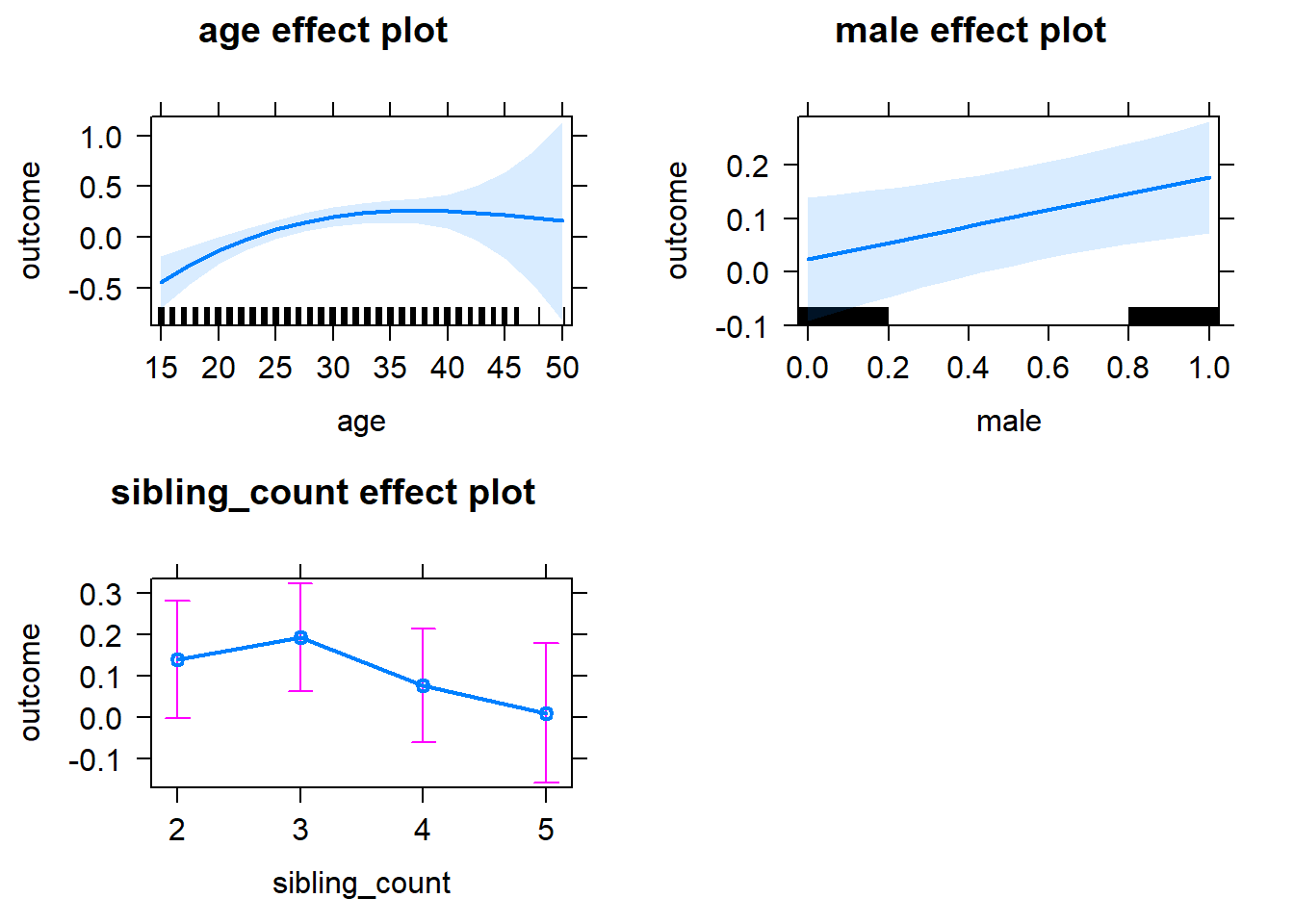
Add Birth Order Linear
Model Summary
tidy(m2_birthorder_linear, conf.int = T, conf.level = 0.995)| effect | group | term | estimate | std.error | statistic | df | p.value | conf.low | conf.high |
|---|---|---|---|---|---|---|---|---|---|
| fixed | NA | (Intercept) | -2.255 | 1.071 | -2.106 | 1878 | 0.03534 | -5.26 | 0.7505 |
| fixed | NA | birth_order | 0.03011 | 0.02277 | 1.322 | 1828 | 0.1862 | -0.0338 | 0.09401 |
| fixed | NA | poly(age, 3, raw = TRUE)1 | 0.1589 | 0.117 | 1.358 | 1879 | 0.1747 | -0.1696 | 0.4874 |
| fixed | NA | poly(age, 3, raw = TRUE)2 | -0.003371 | 0.004111 | -0.82 | 1880 | 0.4123 | -0.01491 | 0.008169 |
| fixed | NA | poly(age, 3, raw = TRUE)3 | 0.00002261 | 0.00004642 | 0.4871 | 1880 | 0.6262 | -0.0001077 | 0.0001529 |
| fixed | NA | male | 0.1525 | 0.04495 | 3.394 | 1893 | 0.0007037 | 0.02637 | 0.2787 |
| fixed | NA | sibling_count3 | 0.03917 | 0.06174 | 0.6345 | 1537 | 0.5259 | -0.1341 | 0.2125 |
| fixed | NA | sibling_count4 | -0.09368 | 0.06713 | -1.395 | 1508 | 0.1631 | -0.2821 | 0.09476 |
| fixed | NA | sibling_count5 | -0.1829 | 0.08224 | -2.224 | 1490 | 0.02632 | -0.4137 | 0.04798 |
| ran_pars | mother_pidlink | sd__(Intercept) | 0.2564 | NA | NA | NA | NA | NA | NA |
| ran_pars | Residual | sd__Observation | 0.9257 | NA | NA | NA | NA | NA | NA |
Coefficient Plot
plot_birthorder2(m2_birthorder_linear, separate = FALSE)
Add Birth Order Factor
Model Summary
m3_birthorder_nonlinear = update(m1_covariates_only, formula = . ~ . + birth_order_nonlinear)
tidy(m3_birthorder_nonlinear, conf.int = T, conf.level = 0.995)| effect | group | term | estimate | std.error | statistic | df | p.value | conf.low | conf.high |
|---|---|---|---|---|---|---|---|---|---|
| fixed | NA | (Intercept) | -2.248 | 1.072 | -2.097 | 1874 | 0.03612 | -5.258 | 0.7611 |
| fixed | NA | poly(age, 3, raw = TRUE)1 | 0.1611 | 0.1172 | 1.374 | 1876 | 0.1696 | -0.168 | 0.4902 |
| fixed | NA | poly(age, 3, raw = TRUE)2 | -0.003454 | 0.004118 | -0.8389 | 1877 | 0.4017 | -0.01501 | 0.008104 |
| fixed | NA | poly(age, 3, raw = TRUE)3 | 0.00002356 | 0.00004649 | 0.5068 | 1877 | 0.6124 | -0.0001069 | 0.000154 |
| fixed | NA | male | 0.1525 | 0.04499 | 3.391 | 1890 | 0.0007115 | 0.02626 | 0.2788 |
| fixed | NA | sibling_count3 | 0.02772 | 0.06268 | 0.4422 | 1577 | 0.6584 | -0.1482 | 0.2037 |
| fixed | NA | sibling_count4 | -0.1077 | 0.06814 | -1.581 | 1552 | 0.114 | -0.299 | 0.08351 |
| fixed | NA | sibling_count5 | -0.1635 | 0.08373 | -1.953 | 1509 | 0.05104 | -0.3985 | 0.07153 |
| fixed | NA | birth_order_nonlinear2 | 0.05357 | 0.05383 | 0.9952 | 1631 | 0.3198 | -0.09753 | 0.2047 |
| fixed | NA | birth_order_nonlinear3 | 0.1133 | 0.06673 | 1.697 | 1708 | 0.08982 | -0.07405 | 0.3006 |
| fixed | NA | birth_order_nonlinear4 | 0.1079 | 0.0884 | 1.221 | 1745 | 0.2222 | -0.1402 | 0.3561 |
| fixed | NA | birth_order_nonlinear5 | -0.02124 | 0.137 | -0.155 | 1793 | 0.8769 | -0.4059 | 0.3635 |
| ran_pars | mother_pidlink | sd__(Intercept) | 0.2587 | NA | NA | NA | NA | NA | NA |
| ran_pars | Residual | sd__Observation | 0.9253 | NA | NA | NA | NA | NA | NA |
Coefficient Plot
plot_birthorder(m3_birthorder_nonlinear, separate = FALSE)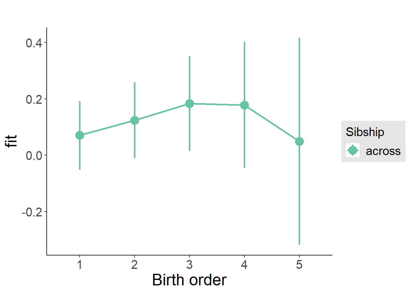
Add Interaction
Model Summary
m4_interaction = update(m3_birthorder_nonlinear, formula = . ~ . - birth_order_nonlinear - sibling_count + count_birth_order)
tidy(m4_interaction, conf.int = T, conf.level = 0.995)| effect | group | term | estimate | std.error | statistic | df | p.value | conf.low | conf.high |
|---|---|---|---|---|---|---|---|---|---|
| fixed | NA | (Intercept) | -2.207 | 1.074 | -2.054 | 1869 | 0.04012 | -5.222 | 0.809 |
| fixed | NA | poly(age, 3, raw = TRUE)1 | 0.1576 | 0.1176 | 1.34 | 1871 | 0.1805 | -0.1726 | 0.4877 |
| fixed | NA | poly(age, 3, raw = TRUE)2 | -0.003291 | 0.004131 | -0.7966 | 1871 | 0.4258 | -0.01489 | 0.008305 |
| fixed | NA | poly(age, 3, raw = TRUE)3 | 0.0000213 | 0.00004664 | 0.4567 | 1872 | 0.6479 | -0.0001096 | 0.0001522 |
| fixed | NA | male | 0.1514 | 0.04506 | 3.359 | 1883 | 0.0007975 | 0.02488 | 0.2779 |
| fixed | NA | count_birth_order2/2 | -0.01058 | 0.09597 | -0.1102 | 1659 | 0.9123 | -0.28 | 0.2588 |
| fixed | NA | count_birth_order1/3 | 0.001797 | 0.07979 | 0.02252 | 1886 | 0.982 | -0.2222 | 0.2258 |
| fixed | NA | count_birth_order2/3 | 0.08769 | 0.0904 | 0.9701 | 1886 | 0.3321 | -0.1661 | 0.3414 |
| fixed | NA | count_birth_order3/3 | 0.09682 | 0.09987 | 0.9695 | 1883 | 0.3324 | -0.1835 | 0.3772 |
| fixed | NA | count_birth_order1/4 | -0.2027 | 0.09365 | -2.164 | 1887 | 0.03058 | -0.4656 | 0.06021 |
| fixed | NA | count_birth_order2/4 | -0.03414 | 0.09687 | -0.3524 | 1886 | 0.7246 | -0.306 | 0.2378 |
| fixed | NA | count_birth_order3/4 | 0.04422 | 0.1022 | 0.4326 | 1882 | 0.6653 | -0.2427 | 0.3311 |
| fixed | NA | count_birth_order4/4 | -0.03093 | 0.1094 | -0.2827 | 1880 | 0.7774 | -0.3381 | 0.2762 |
| fixed | NA | count_birth_order1/5 | -0.0792 | 0.1269 | -0.624 | 1887 | 0.5327 | -0.4355 | 0.2771 |
| fixed | NA | count_birth_order2/5 | -0.2197 | 0.1478 | -1.486 | 1878 | 0.1374 | -0.6346 | 0.1952 |
| fixed | NA | count_birth_order3/5 | -0.1384 | 0.1324 | -1.046 | 1884 | 0.2959 | -0.5099 | 0.2331 |
| fixed | NA | count_birth_order4/5 | -0.0589 | 0.1257 | -0.4685 | 1880 | 0.6395 | -0.4118 | 0.294 |
| fixed | NA | count_birth_order5/5 | -0.2059 | 0.1296 | -1.589 | 1881 | 0.1121 | -0.5696 | 0.1578 |
| ran_pars | mother_pidlink | sd__(Intercept) | 0.2667 | NA | NA | NA | NA | NA | NA |
| ran_pars | Residual | sd__Observation | 0.9236 | NA | NA | NA | NA | NA | NA |
Coefficient Plot
plot_birthorder(m4_interaction)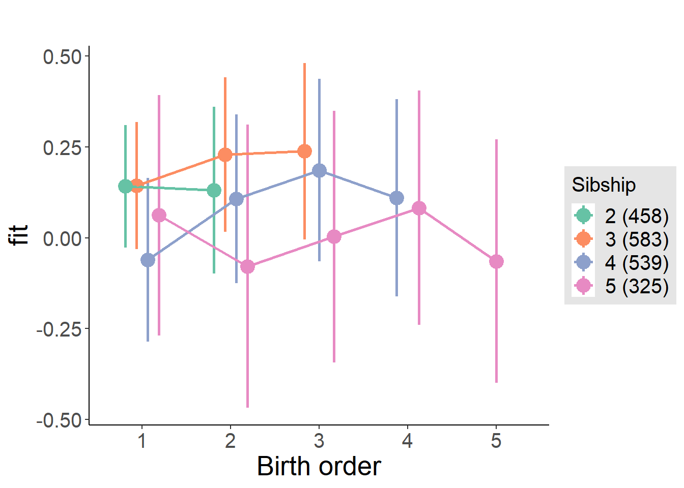
Model Comparison
###### Model 1 - Model 2
anova(m1_covariates_only, m2_birthorder_linear, m3_birthorder_nonlinear, m4_interaction)## refitting model(s) with ML (instead of REML)| Df | AIC | BIC | logLik | deviance | Chisq | Chi Df | Pr(>Chisq) |
|---|---|---|---|---|---|---|---|
| 10 | 5263 | 5319 | -2622 | 5243 | NA | NA | NA |
| 11 | 5263 | 5325 | -2621 | 5241 | 1.747 | 1 | 0.1863 |
| 14 | 5267 | 5345 | -2620 | 5239 | 2.254 | 3 | 0.5215 |
| 20 | 5275 | 5386 | -2618 | 5235 | 4.102 | 6 | 0.6628 |
Maternal pregnancy order
outcome_preg_m1 <- update(m2_birthorder_linear, data = birthorder %>%
mutate(sibling_count = sibling_count_uterus_preg_factor,
birth_order_nonlinear = birthorder_uterus_preg_factor,
birth_order = birthorder_uterus_preg,
count_birth_order = count_birthorder_uterus_preg
) %>%
filter(sibling_count != "1"))
compare_models_markdown(outcome_preg_m1)Basic Model
Model Summary
m1_covariates_only <- update(m2_birthorder_linear, formula = . ~ . - birth_order)
tidy(m1_covariates_only, conf.int = T, conf.level = 0.995)| effect | group | term | estimate | std.error | statistic | df | p.value | conf.low | conf.high |
|---|---|---|---|---|---|---|---|---|---|
| fixed | NA | (Intercept) | -2.248 | 1.099 | -2.045 | 1736 | 0.04101 | -5.334 | 0.8377 |
| fixed | NA | poly(age, 3, raw = TRUE)1 | 0.1627 | 0.1203 | 1.353 | 1738 | 0.1763 | -0.1749 | 0.5002 |
| fixed | NA | poly(age, 3, raw = TRUE)2 | -0.003424 | 0.004223 | -0.8107 | 1739 | 0.4176 | -0.01528 | 0.008431 |
| fixed | NA | poly(age, 3, raw = TRUE)3 | 0.00002166 | 0.00004767 | 0.4543 | 1740 | 0.6497 | -0.0001122 | 0.0001555 |
| fixed | NA | male | 0.1355 | 0.04645 | 2.916 | 1746 | 0.003589 | 0.005067 | 0.2659 |
| fixed | NA | sibling_count3 | 0.03395 | 0.06671 | 0.5089 | 1436 | 0.6109 | -0.1533 | 0.2212 |
| fixed | NA | sibling_count4 | -0.003585 | 0.06781 | -0.05286 | 1363 | 0.9579 | -0.1939 | 0.1868 |
| fixed | NA | sibling_count5 | -0.1122 | 0.07149 | -1.569 | 1266 | 0.1168 | -0.3129 | 0.08848 |
| ran_pars | mother_pidlink | sd__(Intercept) | 0.2856 | NA | NA | NA | NA | NA | NA |
| ran_pars | Residual | sd__Observation | 0.91 | NA | NA | NA | NA | NA | NA |
Coefficient Plot
plot(allEffects(m1_covariates_only, confidence.level = 0.995))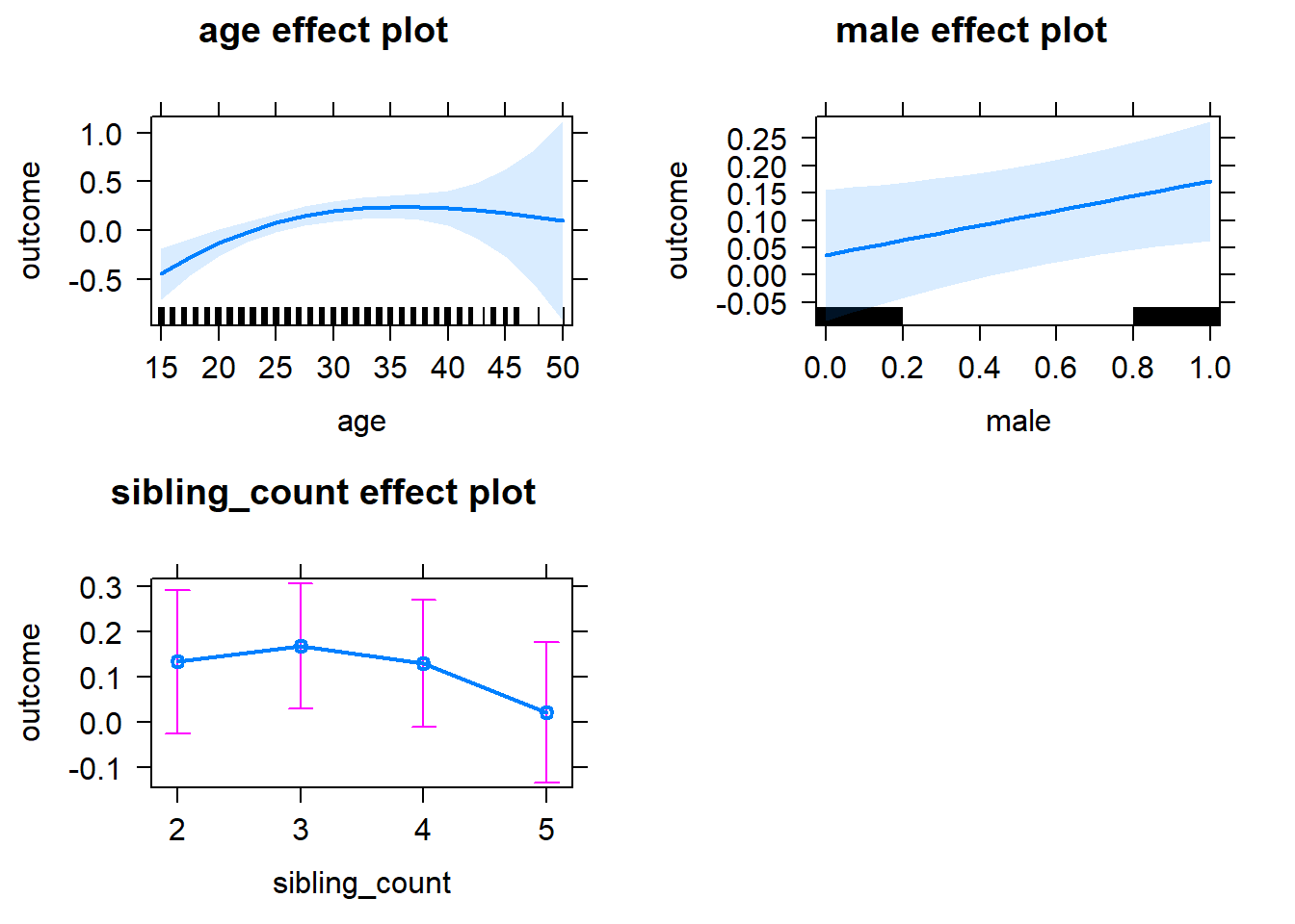
Add Birth Order Linear
Model Summary
tidy(m2_birthorder_linear, conf.int = T, conf.level = 0.995)| effect | group | term | estimate | std.error | statistic | df | p.value | conf.low | conf.high |
|---|---|---|---|---|---|---|---|---|---|
| fixed | NA | (Intercept) | -2.276 | 1.1 | -2.07 | 1736 | 0.0386 | -5.363 | 0.8105 |
| fixed | NA | birth_order | 0.02453 | 0.02258 | 1.086 | 1706 | 0.2775 | -0.03886 | 0.08792 |
| fixed | NA | poly(age, 3, raw = TRUE)1 | 0.1628 | 0.1203 | 1.354 | 1738 | 0.1759 | -0.1747 | 0.5004 |
| fixed | NA | poly(age, 3, raw = TRUE)2 | -0.003461 | 0.004223 | -0.8196 | 1739 | 0.4126 | -0.01532 | 0.008393 |
| fixed | NA | poly(age, 3, raw = TRUE)3 | 0.00002261 | 0.00004768 | 0.4743 | 1740 | 0.6354 | -0.0001112 | 0.0001564 |
| fixed | NA | male | 0.1354 | 0.04645 | 2.915 | 1745 | 0.003601 | 0.00502 | 0.2658 |
| fixed | NA | sibling_count3 | 0.02227 | 0.06758 | 0.3296 | 1448 | 0.7418 | -0.1674 | 0.212 |
| fixed | NA | sibling_count4 | -0.02785 | 0.07142 | -0.3899 | 1426 | 0.6967 | -0.2283 | 0.1726 |
| fixed | NA | sibling_count5 | -0.1518 | 0.0803 | -1.891 | 1411 | 0.05882 | -0.3772 | 0.07355 |
| ran_pars | mother_pidlink | sd__(Intercept) | 0.2891 | NA | NA | NA | NA | NA | NA |
| ran_pars | Residual | sd__Observation | 0.9089 | NA | NA | NA | NA | NA | NA |
Coefficient Plot
plot_birthorder2(m2_birthorder_linear, separate = FALSE)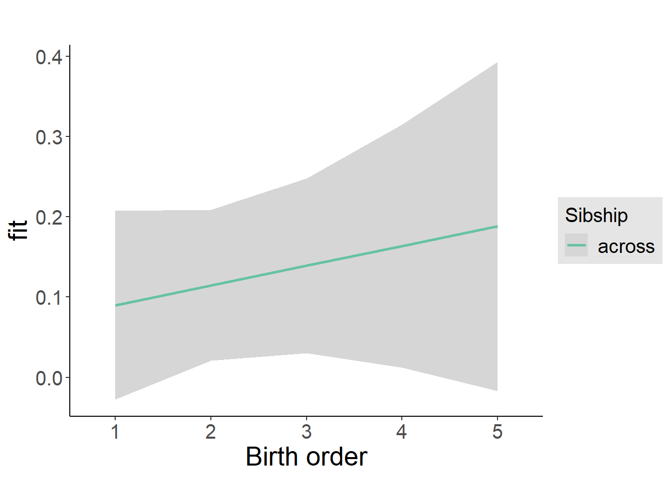
Add Birth Order Factor
Model Summary
m3_birthorder_nonlinear = update(m1_covariates_only, formula = . ~ . + birth_order_nonlinear)
tidy(m3_birthorder_nonlinear, conf.int = T, conf.level = 0.995)| effect | group | term | estimate | std.error | statistic | df | p.value | conf.low | conf.high |
|---|---|---|---|---|---|---|---|---|---|
| fixed | NA | (Intercept) | -2.265 | 1.101 | -2.056 | 1731 | 0.03989 | -5.357 | 0.8268 |
| fixed | NA | poly(age, 3, raw = TRUE)1 | 0.1629 | 0.1205 | 1.352 | 1734 | 0.1765 | -0.1753 | 0.5012 |
| fixed | NA | poly(age, 3, raw = TRUE)2 | -0.003483 | 0.004232 | -0.8231 | 1735 | 0.4106 | -0.01536 | 0.008396 |
| fixed | NA | poly(age, 3, raw = TRUE)3 | 0.00002298 | 0.00004777 | 0.4811 | 1735 | 0.6305 | -0.0001111 | 0.0001571 |
| fixed | NA | male | 0.1348 | 0.0465 | 2.899 | 1742 | 0.003786 | 0.004293 | 0.2654 |
| fixed | NA | sibling_count3 | 0.01432 | 0.06858 | 0.2088 | 1478 | 0.8346 | -0.1782 | 0.2068 |
| fixed | NA | sibling_count4 | -0.04198 | 0.07236 | -0.5801 | 1458 | 0.562 | -0.2451 | 0.1612 |
| fixed | NA | sibling_count5 | -0.1367 | 0.08086 | -1.691 | 1416 | 0.09111 | -0.3637 | 0.09026 |
| fixed | NA | birth_order_nonlinear2 | 0.08313 | 0.05537 | 1.501 | 1501 | 0.1335 | -0.07229 | 0.2386 |
| fixed | NA | birth_order_nonlinear3 | 0.08249 | 0.06895 | 1.196 | 1599 | 0.2317 | -0.111 | 0.276 |
| fixed | NA | birth_order_nonlinear4 | 0.1182 | 0.08989 | 1.315 | 1605 | 0.1886 | -0.1341 | 0.3705 |
| fixed | NA | birth_order_nonlinear5 | -0.02157 | 0.1279 | -0.1686 | 1645 | 0.8661 | -0.3807 | 0.3376 |
| ran_pars | mother_pidlink | sd__(Intercept) | 0.2903 | NA | NA | NA | NA | NA | NA |
| ran_pars | Residual | sd__Observation | 0.9086 | NA | NA | NA | NA | NA | NA |
Coefficient Plot
plot_birthorder(m3_birthorder_nonlinear, separate = FALSE)
Add Interaction
Model Summary
m4_interaction = update(m3_birthorder_nonlinear, formula = . ~ . - birth_order_nonlinear - sibling_count + count_birth_order)
tidy(m4_interaction, conf.int = T, conf.level = 0.995)| effect | group | term | estimate | std.error | statistic | df | p.value | conf.low | conf.high |
|---|---|---|---|---|---|---|---|---|---|
| fixed | NA | (Intercept) | -2.226 | 1.106 | -2.012 | 1726 | 0.04437 | -5.331 | 0.8794 |
| fixed | NA | poly(age, 3, raw = TRUE)1 | 0.1608 | 0.1211 | 1.328 | 1728 | 0.1844 | -0.1792 | 0.5008 |
| fixed | NA | poly(age, 3, raw = TRUE)2 | -0.003377 | 0.004253 | -0.7942 | 1729 | 0.4272 | -0.01531 | 0.00856 |
| fixed | NA | poly(age, 3, raw = TRUE)3 | 0.00002152 | 0.000048 | 0.4483 | 1730 | 0.654 | -0.0001132 | 0.0001563 |
| fixed | NA | male | 0.1357 | 0.04665 | 2.909 | 1735 | 0.003676 | 0.004742 | 0.2667 |
| fixed | NA | count_birth_order2/2 | -0.01203 | 0.1074 | -0.112 | 1573 | 0.9108 | -0.3135 | 0.2894 |
| fixed | NA | count_birth_order1/3 | -0.03039 | 0.08738 | -0.3478 | 1741 | 0.7281 | -0.2757 | 0.2149 |
| fixed | NA | count_birth_order2/3 | 0.1045 | 0.0968 | 1.079 | 1742 | 0.2806 | -0.1672 | 0.3762 |
| fixed | NA | count_birth_order3/3 | 0.04883 | 0.1086 | 0.4495 | 1739 | 0.6531 | -0.2561 | 0.3537 |
| fixed | NA | count_birth_order1/4 | -0.1154 | 0.09836 | -1.173 | 1742 | 0.2409 | -0.3915 | 0.1607 |
| fixed | NA | count_birth_order2/4 | 0.06725 | 0.09911 | 0.6785 | 1741 | 0.4975 | -0.2109 | 0.3454 |
| fixed | NA | count_birth_order3/4 | 0.01112 | 0.1112 | 0.1 | 1737 | 0.9203 | -0.3009 | 0.3232 |
| fixed | NA | count_birth_order4/4 | 0.02798 | 0.1189 | 0.2353 | 1732 | 0.814 | -0.3058 | 0.3617 |
| fixed | NA | count_birth_order1/5 | -0.1351 | 0.1149 | -1.176 | 1742 | 0.2397 | -0.4575 | 0.1873 |
| fixed | NA | count_birth_order2/5 | -0.1738 | 0.1263 | -1.376 | 1734 | 0.1689 | -0.5282 | 0.1806 |
| fixed | NA | count_birth_order3/5 | -0.05605 | 0.1259 | -0.445 | 1734 | 0.6563 | -0.4096 | 0.2975 |
| fixed | NA | count_birth_order4/5 | -0.02405 | 0.1267 | -0.1898 | 1727 | 0.8495 | -0.3798 | 0.3317 |
| fixed | NA | count_birth_order5/5 | -0.1875 | 0.1263 | -1.484 | 1732 | 0.1379 | -0.5419 | 0.167 |
| ran_pars | mother_pidlink | sd__(Intercept) | 0.3023 | NA | NA | NA | NA | NA | NA |
| ran_pars | Residual | sd__Observation | 0.9058 | NA | NA | NA | NA | NA | NA |
Coefficient Plot
plot_birthorder(m4_interaction)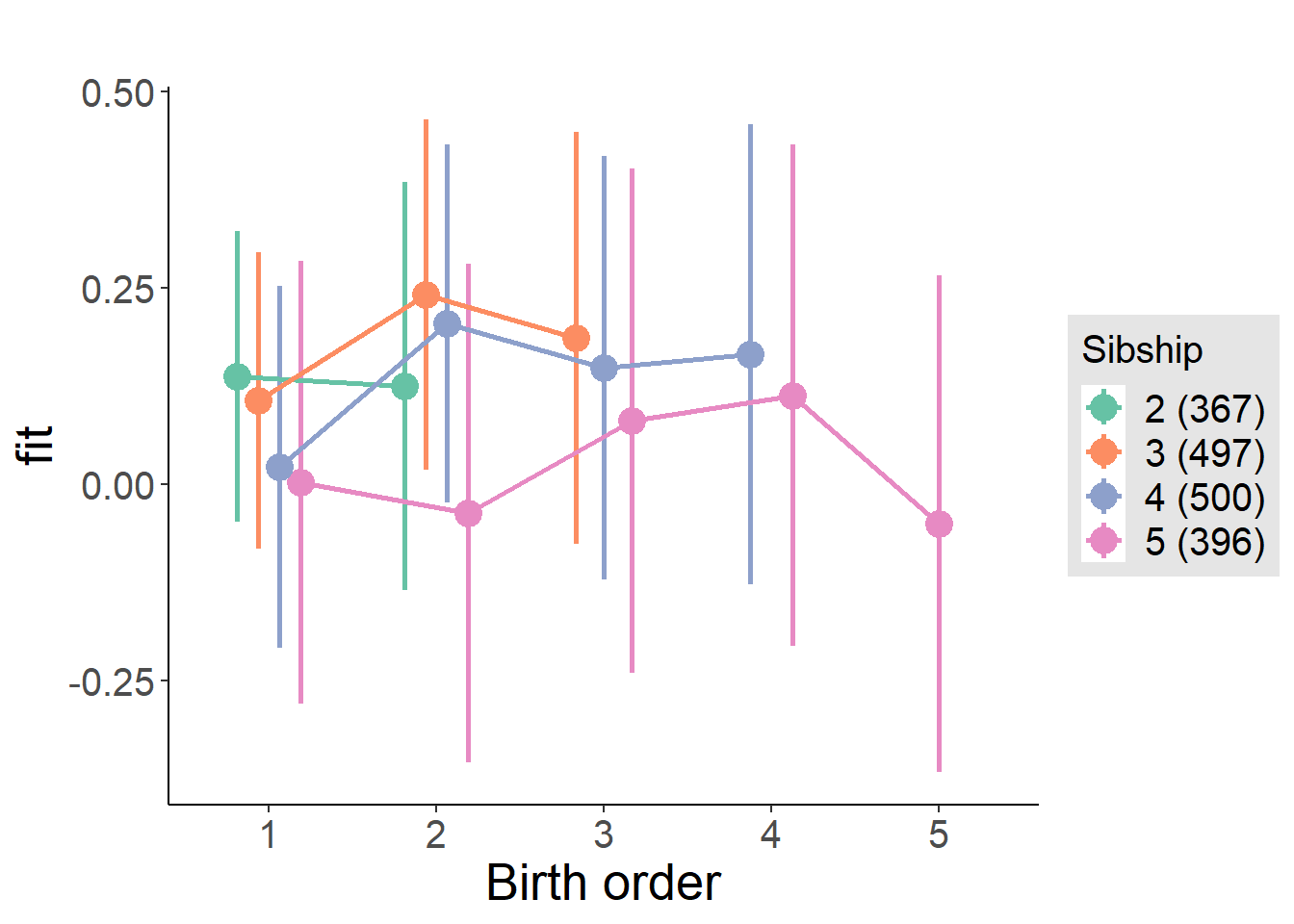
Model Comparison
###### Model 1 - Model 2
anova(m1_covariates_only, m2_birthorder_linear, m3_birthorder_nonlinear, m4_interaction)## refitting model(s) with ML (instead of REML)| Df | AIC | BIC | logLik | deviance | Chisq | Chi Df | Pr(>Chisq) |
|---|---|---|---|---|---|---|---|
| 10 | 4837 | 4891 | -2408 | 4817 | NA | NA | NA |
| 11 | 4838 | 4898 | -2408 | 4816 | 1.179 | 1 | 0.2776 |
| 14 | 4841 | 4917 | -2406 | 4813 | 2.727 | 3 | 0.4356 |
| 20 | 4850 | 4959 | -2405 | 4810 | 2.944 | 6 | 0.8158 |
Parental full sibling order
outcome_parental_m1 <- update(m2_birthorder_linear, data = birthorder %>%
mutate(sibling_count = sibling_count_genes_factor,
birth_order_nonlinear = birthorder_genes_factor,
birth_order = birthorder_genes,
count_birth_order = count_birthorder_genes
) %>%
filter(sibling_count != "1"))
compare_models_markdown(outcome_parental_m1)Basic Model
Model Summary
m1_covariates_only <- update(m2_birthorder_linear, formula = . ~ . - birth_order)
tidy(m1_covariates_only, conf.int = T, conf.level = 0.995)| effect | group | term | estimate | std.error | statistic | df | p.value | conf.low | conf.high |
|---|---|---|---|---|---|---|---|---|---|
| fixed | NA | (Intercept) | -2.117 | 1.094 | -1.935 | 1867 | 0.05316 | -5.189 | 0.9544 |
| fixed | NA | poly(age, 3, raw = TRUE)1 | 0.1426 | 0.1197 | 1.192 | 1869 | 0.2335 | -0.1933 | 0.4786 |
| fixed | NA | poly(age, 3, raw = TRUE)2 | -0.002663 | 0.004203 | -0.6336 | 1869 | 0.5264 | -0.01446 | 0.009135 |
| fixed | NA | poly(age, 3, raw = TRUE)3 | 0.00001294 | 0.00004745 | 0.2727 | 1869 | 0.7851 | -0.0001203 | 0.0001461 |
| fixed | NA | male | 0.1735 | 0.04603 | 3.769 | 1883 | 0.0001692 | 0.04426 | 0.3027 |
| fixed | NA | sibling_count3 | 0.04045 | 0.06137 | 0.6591 | 1506 | 0.51 | -0.1318 | 0.2127 |
| fixed | NA | sibling_count4 | -0.08907 | 0.0641 | -1.389 | 1384 | 0.1649 | -0.269 | 0.09087 |
| fixed | NA | sibling_count5 | -0.1029 | 0.07522 | -1.368 | 1229 | 0.1715 | -0.3141 | 0.1082 |
| ran_pars | mother_pidlink | sd__(Intercept) | 0.2642 | NA | NA | NA | NA | NA | NA |
| ran_pars | Residual | sd__Observation | 0.9458 | NA | NA | NA | NA | NA | NA |
Coefficient Plot
plot(allEffects(m1_covariates_only, confidence.level = 0.995))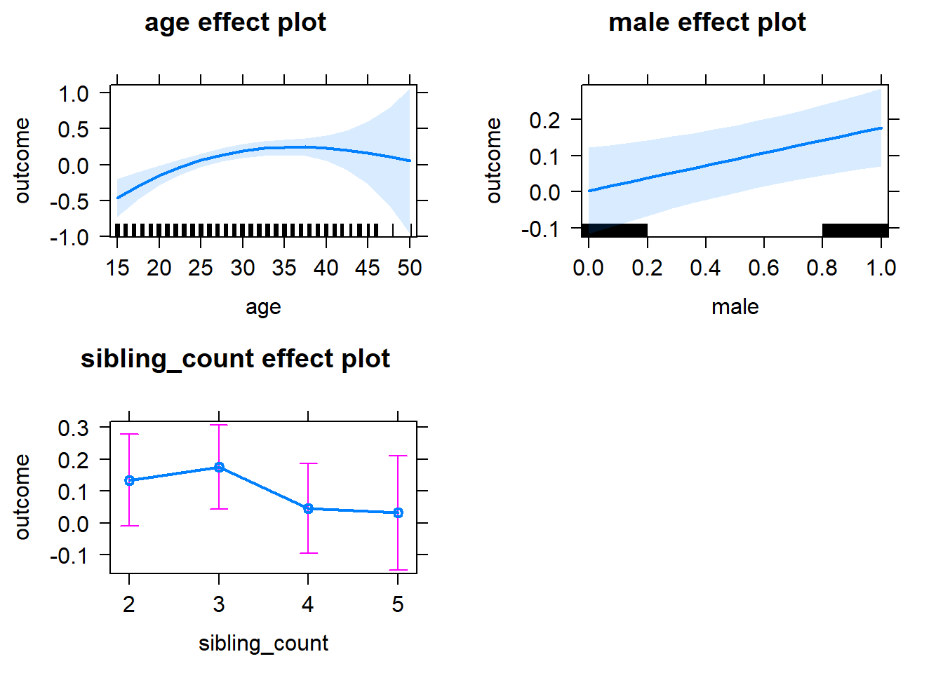
Add Birth Order Linear
Model Summary
tidy(m2_birthorder_linear, conf.int = T, conf.level = 0.995)| effect | group | term | estimate | std.error | statistic | df | p.value | conf.low | conf.high |
|---|---|---|---|---|---|---|---|---|---|
| fixed | NA | (Intercept) | -2.13 | 1.094 | -1.946 | 1867 | 0.05175 | -5.202 | 0.9418 |
| fixed | NA | birth_order | 0.02341 | 0.0237 | 0.9875 | 1802 | 0.3235 | -0.04312 | 0.08994 |
| fixed | NA | poly(age, 3, raw = TRUE)1 | 0.1415 | 0.1197 | 1.182 | 1868 | 0.2372 | -0.1944 | 0.4775 |
| fixed | NA | poly(age, 3, raw = TRUE)2 | -0.002663 | 0.004203 | -0.6335 | 1869 | 0.5265 | -0.01446 | 0.009136 |
| fixed | NA | poly(age, 3, raw = TRUE)3 | 0.00001349 | 0.00004746 | 0.2842 | 1869 | 0.7763 | -0.0001197 | 0.0001467 |
| fixed | NA | male | 0.173 | 0.04603 | 3.759 | 1882 | 0.0001758 | 0.04382 | 0.3022 |
| fixed | NA | sibling_count3 | 0.02954 | 0.06238 | 0.4736 | 1524 | 0.6359 | -0.1456 | 0.2046 |
| fixed | NA | sibling_count4 | -0.1128 | 0.06847 | -1.647 | 1494 | 0.09976 | -0.305 | 0.07942 |
| fixed | NA | sibling_count5 | -0.1428 | 0.08544 | -1.671 | 1425 | 0.09484 | -0.3826 | 0.09702 |
| ran_pars | mother_pidlink | sd__(Intercept) | 0.2671 | NA | NA | NA | NA | NA | NA |
| ran_pars | Residual | sd__Observation | 0.9451 | NA | NA | NA | NA | NA | NA |
Coefficient Plot
plot_birthorder2(m2_birthorder_linear, separate = FALSE)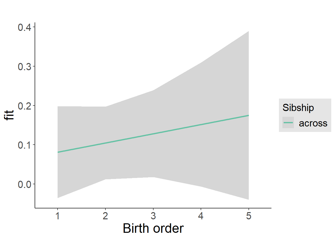
Add Birth Order Factor
Model Summary
m3_birthorder_nonlinear = update(m1_covariates_only, formula = . ~ . + birth_order_nonlinear)
tidy(m3_birthorder_nonlinear, conf.int = T, conf.level = 0.995)| effect | group | term | estimate | std.error | statistic | df | p.value | conf.low | conf.high |
|---|---|---|---|---|---|---|---|---|---|
| fixed | NA | (Intercept) | -2.191 | 1.096 | -1.999 | 1863 | 0.04575 | -5.267 | 0.8854 |
| fixed | NA | poly(age, 3, raw = TRUE)1 | 0.1507 | 0.1199 | 1.257 | 1864 | 0.209 | -0.1858 | 0.4872 |
| fixed | NA | poly(age, 3, raw = TRUE)2 | -0.002995 | 0.00421 | -0.7115 | 1865 | 0.4769 | -0.01481 | 0.008821 |
| fixed | NA | poly(age, 3, raw = TRUE)3 | 0.00001717 | 0.00004753 | 0.3613 | 1865 | 0.7179 | -0.0001162 | 0.0001506 |
| fixed | NA | male | 0.1749 | 0.0461 | 3.794 | 1880 | 0.000153 | 0.04549 | 0.3043 |
| fixed | NA | sibling_count3 | 0.009642 | 0.06337 | 0.1522 | 1565 | 0.8791 | -0.1682 | 0.1875 |
| fixed | NA | sibling_count4 | -0.1218 | 0.0694 | -1.755 | 1539 | 0.07946 | -0.3166 | 0.07301 |
| fixed | NA | sibling_count5 | -0.1235 | 0.08717 | -1.417 | 1453 | 0.1566 | -0.3682 | 0.1211 |
| fixed | NA | birth_order_nonlinear2 | 0.04081 | 0.05474 | 0.7455 | 1614 | 0.4561 | -0.1128 | 0.1945 |
| fixed | NA | birth_order_nonlinear3 | 0.1357 | 0.06808 | 1.993 | 1700 | 0.04643 | -0.05542 | 0.3268 |
| fixed | NA | birth_order_nonlinear4 | 0.017 | 0.09331 | 0.1821 | 1712 | 0.8555 | -0.2449 | 0.2789 |
| fixed | NA | birth_order_nonlinear5 | -0.01179 | 0.1488 | -0.07925 | 1776 | 0.9368 | -0.4293 | 0.4058 |
| ran_pars | mother_pidlink | sd__(Intercept) | 0.2666 | NA | NA | NA | NA | NA | NA |
| ran_pars | Residual | sd__Observation | 0.9451 | NA | NA | NA | NA | NA | NA |
Coefficient Plot
plot_birthorder(m3_birthorder_nonlinear, separate = FALSE)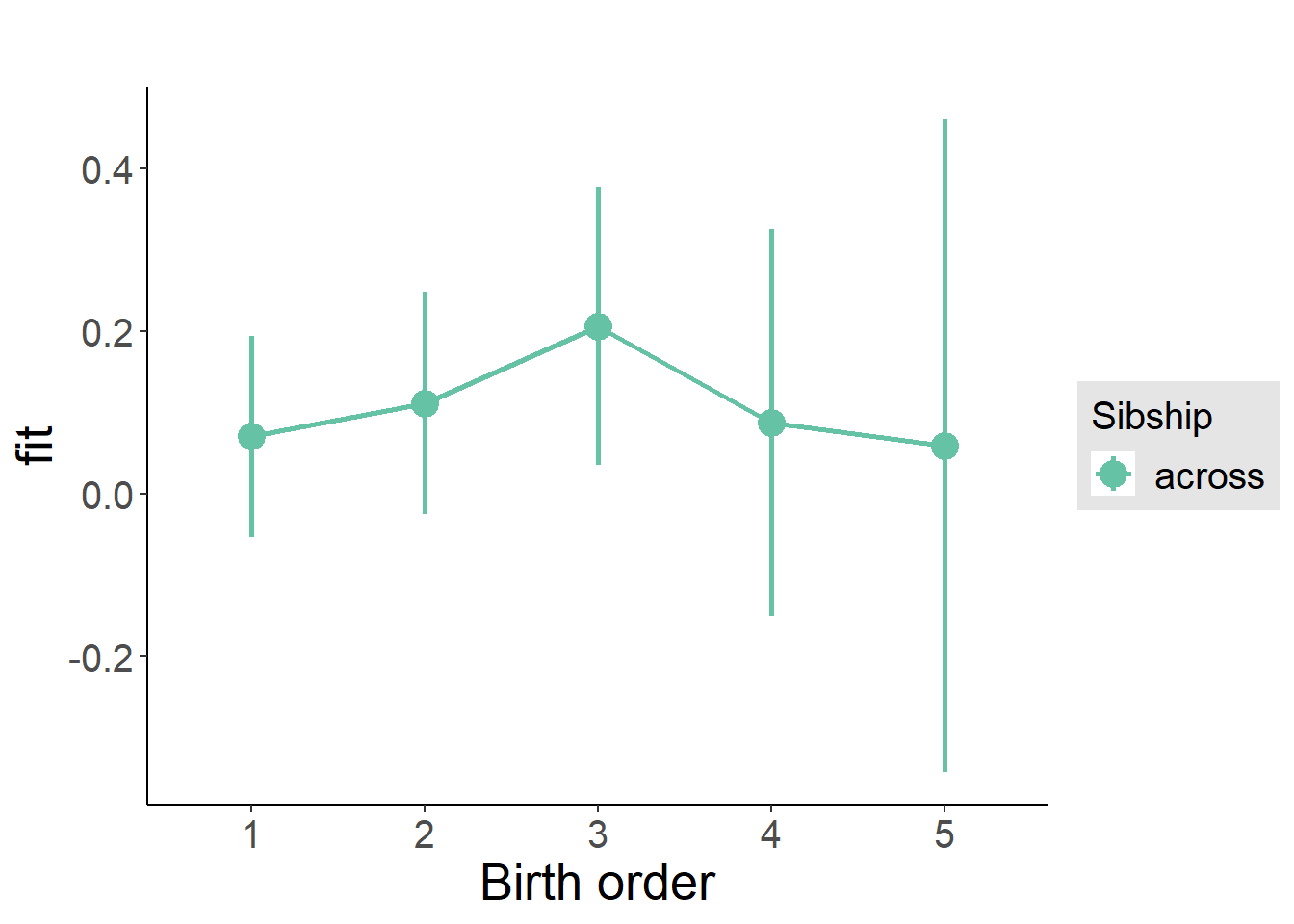
Add Interaction
Model Summary
m4_interaction = update(m3_birthorder_nonlinear, formula = . ~ . - birth_order_nonlinear - sibling_count + count_birth_order)
tidy(m4_interaction, conf.int = T, conf.level = 0.995)| effect | group | term | estimate | std.error | statistic | df | p.value | conf.low | conf.high |
|---|---|---|---|---|---|---|---|---|---|
| fixed | NA | (Intercept) | -2.206 | 1.098 | -2.009 | 1857 | 0.04473 | -5.288 | 0.8769 |
| fixed | NA | poly(age, 3, raw = TRUE)1 | 0.1549 | 0.1203 | 1.288 | 1859 | 0.1979 | -0.1827 | 0.4926 |
| fixed | NA | poly(age, 3, raw = TRUE)2 | -0.003103 | 0.004224 | -0.7346 | 1859 | 0.4627 | -0.01496 | 0.008755 |
| fixed | NA | poly(age, 3, raw = TRUE)3 | 0.000018 | 0.0000477 | 0.3774 | 1860 | 0.7059 | -0.0001159 | 0.0001519 |
| fixed | NA | male | 0.1754 | 0.04618 | 3.799 | 1873 | 0.0001502 | 0.04579 | 0.305 |
| fixed | NA | count_birth_order2/2 | -0.06978 | 0.09583 | -0.7282 | 1627 | 0.4666 | -0.3388 | 0.1992 |
| fixed | NA | count_birth_order1/3 | -0.04446 | 0.08074 | -0.5506 | 1876 | 0.582 | -0.2711 | 0.1822 |
| fixed | NA | count_birth_order2/3 | 0.06535 | 0.09183 | 0.7116 | 1876 | 0.4768 | -0.1924 | 0.3231 |
| fixed | NA | count_birth_order3/3 | 0.0826 | 0.09947 | 0.8305 | 1871 | 0.4064 | -0.1966 | 0.3618 |
| fixed | NA | count_birth_order1/4 | -0.2275 | 0.09624 | -2.364 | 1877 | 0.01819 | -0.4976 | 0.04266 |
| fixed | NA | count_birth_order2/4 | -0.08213 | 0.09867 | -0.8324 | 1875 | 0.4053 | -0.3591 | 0.1948 |
| fixed | NA | count_birth_order3/4 | 0.04063 | 0.1043 | 0.3895 | 1873 | 0.697 | -0.2522 | 0.3335 |
| fixed | NA | count_birth_order4/4 | -0.1586 | 0.1141 | -1.39 | 1868 | 0.1648 | -0.4789 | 0.1617 |
| fixed | NA | count_birth_order1/5 | -0.08721 | 0.1325 | -0.658 | 1877 | 0.5106 | -0.4593 | 0.2849 |
| fixed | NA | count_birth_order2/5 | -0.1772 | 0.1537 | -1.153 | 1870 | 0.2491 | -0.6085 | 0.2542 |
| fixed | NA | count_birth_order3/5 | -0.09323 | 0.1417 | -0.6581 | 1873 | 0.5105 | -0.4909 | 0.3044 |
| fixed | NA | count_birth_order4/5 | -0.1134 | 0.1354 | -0.8372 | 1868 | 0.4026 | -0.4935 | 0.2667 |
| fixed | NA | count_birth_order5/5 | -0.1715 | 0.1402 | -1.223 | 1870 | 0.2215 | -0.5651 | 0.2221 |
| ran_pars | mother_pidlink | sd__(Intercept) | 0.2728 | NA | NA | NA | NA | NA | NA |
| ran_pars | Residual | sd__Observation | 0.9438 | NA | NA | NA | NA | NA | NA |
Coefficient Plot
plot_birthorder(m4_interaction)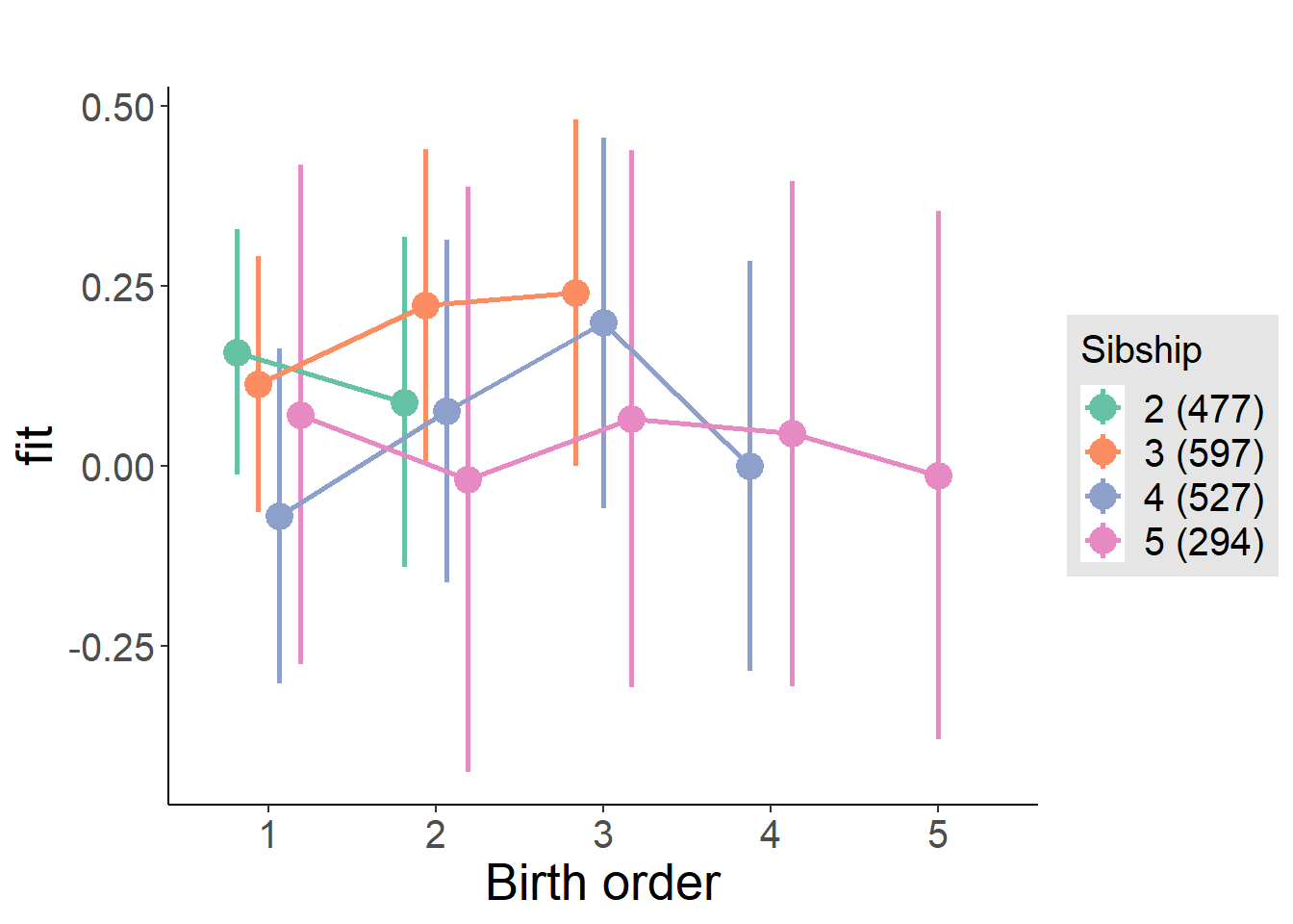
Model Comparison
###### Model 1 - Model 2
anova(m1_covariates_only, m2_birthorder_linear, m3_birthorder_nonlinear, m4_interaction)## refitting model(s) with ML (instead of REML)| Df | AIC | BIC | logLik | deviance | Chisq | Chi Df | Pr(>Chisq) |
|---|---|---|---|---|---|---|---|
| 10 | 5319 | 5374 | -2649 | 5299 | NA | NA | NA |
| 11 | 5320 | 5381 | -2649 | 5298 | 0.9746 | 1 | 0.3235 |
| 14 | 5322 | 5400 | -2647 | 5294 | 3.379 | 3 | 0.3368 |
| 20 | 5330 | 5441 | -2645 | 5290 | 4.503 | 6 | 0.609 |
Compare birth order specifications
library(coefplot)
multiplot(outcome_naive_m1, outcome_preg_m1, outcome_uterus_m1, outcome_parental_m1, dodgeHeight = 0.6,
intercept = FALSE)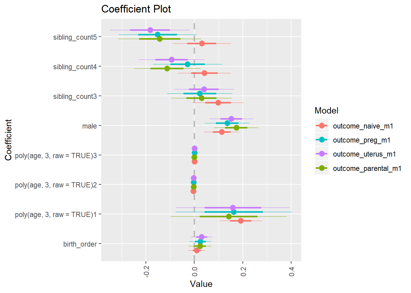
Income last year (log) - z-standardized
birthorder <- birthorder %>% mutate(outcome = wage_last_year_z)
model = lmer(outcome ~ birth_order + poly(age, 3, raw = TRUE) + male + sibling_count + (1 | mother_pidlink),
data = birthorder)
compare_birthorder_specs(model)Naive birth order
outcome_naive_m1 <- update(m2_birthorder_linear, data = birthorder %>%
mutate(sibling_count = sibling_count_naive_factor,
birth_order_nonlinear = birthorder_naive_factor,
birth_order = birthorder_naive,
count_birth_order = count_birthorder_naive) %>%
filter(sibling_count != "1"))
compare_models_markdown(outcome_naive_m1)Basic Model
Model Summary
m1_covariates_only <- update(m2_birthorder_linear, formula = . ~ . - birth_order)
tidy(m1_covariates_only, conf.int = T, conf.level = 0.995)| effect | group | term | estimate | std.error | statistic | df | p.value | conf.low | conf.high |
|---|---|---|---|---|---|---|---|---|---|
| fixed | NA | (Intercept) | -4.289 | 0.4717 | -9.092 | 2886 | 1.758e-19 | -5.613 | -2.965 |
| fixed | NA | poly(age, 3, raw = TRUE)1 | 0.3338 | 0.04424 | 7.546 | 2880 | 5.966e-14 | 0.2097 | 0.458 |
| fixed | NA | poly(age, 3, raw = TRUE)2 | -0.008164 | 0.0013 | -6.28 | 2879 | 0.0000000003898 | -0.01181 | -0.004515 |
| fixed | NA | poly(age, 3, raw = TRUE)3 | 0.00006366 | 0.00001206 | 5.277 | 2885 | 0.0000001412 | 0.0000298 | 0.00009753 |
| fixed | NA | male | 0.1088 | 0.0367 | 2.964 | 2903 | 0.003059 | 0.005768 | 0.2118 |
| fixed | NA | sibling_count3 | 0.07339 | 0.05274 | 1.392 | 2141 | 0.1642 | -0.07465 | 0.2214 |
| fixed | NA | sibling_count4 | 0.03634 | 0.05287 | 0.6872 | 2038 | 0.492 | -0.1121 | 0.1847 |
| fixed | NA | sibling_count5 | 0.02447 | 0.05519 | 0.4433 | 1941 | 0.6576 | -0.1305 | 0.1794 |
| ran_pars | mother_pidlink | sd__(Intercept) | 0.414 | NA | NA | NA | NA | NA | NA |
| ran_pars | Residual | sd__Observation | 0.8867 | NA | NA | NA | NA | NA | NA |
Coefficient Plot
plot(allEffects(m1_covariates_only, confidence.level = 0.995))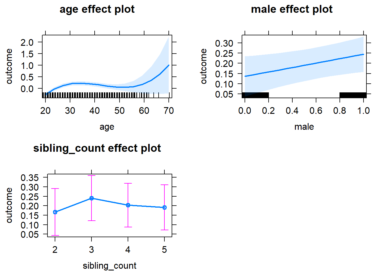
Add Birth Order Linear
Model Summary
tidy(m2_birthorder_linear, conf.int = T, conf.level = 0.995)| effect | group | term | estimate | std.error | statistic | df | p.value | conf.low | conf.high |
|---|---|---|---|---|---|---|---|---|---|
| fixed | NA | (Intercept) | -4.286 | 0.4716 | -9.089 | 2884 | 1.809e-19 | -5.61 | -2.963 |
| fixed | NA | birth_order | -0.02806 | 0.01766 | -1.589 | 2472 | 0.1122 | -0.07762 | 0.0215 |
| fixed | NA | poly(age, 3, raw = TRUE)1 | 0.3368 | 0.04426 | 7.609 | 2879 | 3.718e-14 | 0.2125 | 0.461 |
| fixed | NA | poly(age, 3, raw = TRUE)2 | -0.008225 | 0.0013 | -6.327 | 2877 | 0.0000000002892 | -0.01187 | -0.004576 |
| fixed | NA | poly(age, 3, raw = TRUE)3 | 0.00006393 | 0.00001206 | 5.3 | 2883 | 0.0000001245 | 0.00003007 | 0.00009778 |
| fixed | NA | male | 0.1085 | 0.03669 | 2.956 | 2903 | 0.003139 | 0.005475 | 0.2115 |
| fixed | NA | sibling_count3 | 0.08371 | 0.0531 | 1.576 | 2188 | 0.1151 | -0.06534 | 0.2328 |
| fixed | NA | sibling_count4 | 0.06062 | 0.055 | 1.102 | 2257 | 0.2705 | -0.09376 | 0.215 |
| fixed | NA | sibling_count5 | 0.06253 | 0.06012 | 1.04 | 2368 | 0.2984 | -0.1062 | 0.2313 |
| ran_pars | mother_pidlink | sd__(Intercept) | 0.4114 | NA | NA | NA | NA | NA | NA |
| ran_pars | Residual | sd__Observation | 0.8875 | NA | NA | NA | NA | NA | NA |
Coefficient Plot
plot_birthorder2(m2_birthorder_linear, separate = FALSE)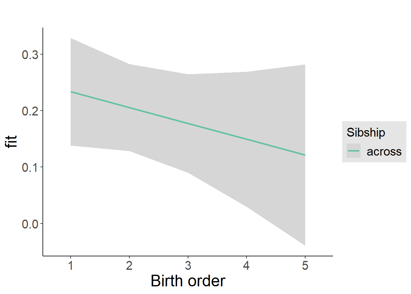
Add Birth Order Factor
Model Summary
m3_birthorder_nonlinear = update(m1_covariates_only, formula = . ~ . + birth_order_nonlinear)
tidy(m3_birthorder_nonlinear, conf.int = T, conf.level = 0.995)| effect | group | term | estimate | std.error | statistic | df | p.value | conf.low | conf.high |
|---|---|---|---|---|---|---|---|---|---|
| fixed | NA | (Intercept) | -4.29 | 0.4727 | -9.076 | 2877 | 2.036e-19 | -5.617 | -2.963 |
| fixed | NA | poly(age, 3, raw = TRUE)1 | 0.3347 | 0.04432 | 7.552 | 2869 | 5.717e-14 | 0.2103 | 0.4591 |
| fixed | NA | poly(age, 3, raw = TRUE)2 | -0.008146 | 0.001303 | -6.253 | 2865 | 0.0000000004625 | -0.0118 | -0.004489 |
| fixed | NA | poly(age, 3, raw = TRUE)3 | 0.00006304 | 0.0000121 | 5.212 | 2868 | 0.0000002005 | 0.00002909 | 0.00009699 |
| fixed | NA | male | 0.109 | 0.03673 | 2.968 | 2903 | 0.003023 | 0.005909 | 0.2121 |
| fixed | NA | sibling_count3 | 0.09064 | 0.05384 | 1.684 | 2269 | 0.09241 | -0.06048 | 0.2418 |
| fixed | NA | sibling_count4 | 0.07197 | 0.05587 | 1.288 | 2344 | 0.1978 | -0.08485 | 0.2288 |
| fixed | NA | sibling_count5 | 0.0541 | 0.06059 | 0.8928 | 2415 | 0.372 | -0.116 | 0.2242 |
| fixed | NA | birth_order_nonlinear2 | -0.05317 | 0.04338 | -1.226 | 2404 | 0.2204 | -0.1749 | 0.06859 |
| fixed | NA | birth_order_nonlinear3 | -0.09253 | 0.05424 | -1.706 | 2358 | 0.08817 | -0.2448 | 0.05973 |
| fixed | NA | birth_order_nonlinear4 | -0.1128 | 0.0697 | -1.619 | 2332 | 0.1056 | -0.3085 | 0.08282 |
| fixed | NA | birth_order_nonlinear5 | -0.01194 | 0.1018 | -0.1173 | 2331 | 0.9066 | -0.2976 | 0.2737 |
| ran_pars | mother_pidlink | sd__(Intercept) | 0.4074 | NA | NA | NA | NA | NA | NA |
| ran_pars | Residual | sd__Observation | 0.8893 | NA | NA | NA | NA | NA | NA |
Coefficient Plot
plot_birthorder(m3_birthorder_nonlinear, separate = FALSE)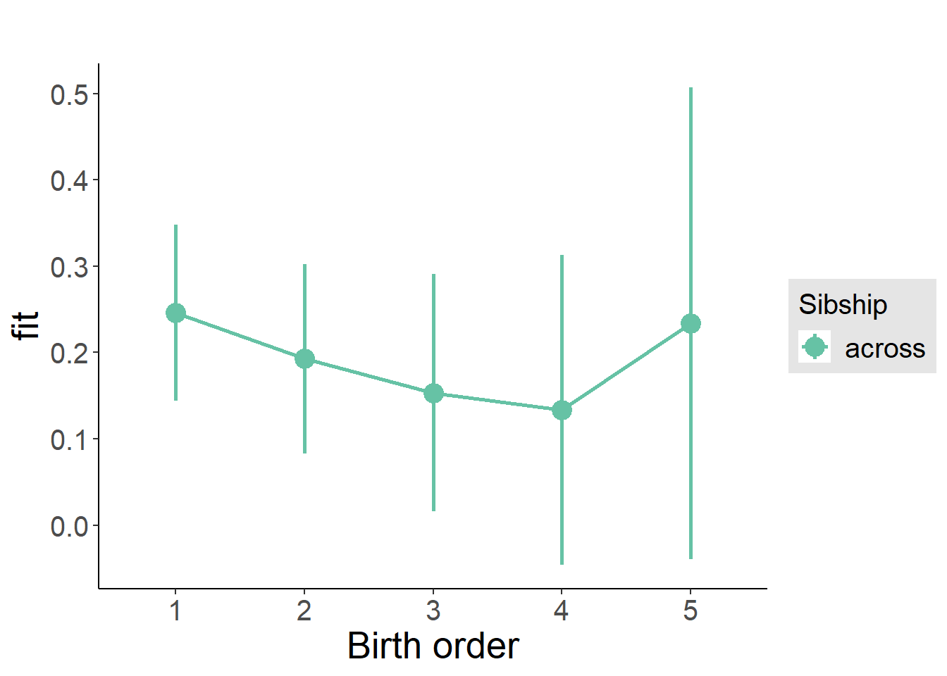
Add Interaction
Model Summary
m4_interaction = update(m3_birthorder_nonlinear, formula = . ~ . - birth_order_nonlinear - sibling_count + count_birth_order)
tidy(m4_interaction, conf.int = T, conf.level = 0.995)| effect | group | term | estimate | std.error | statistic | df | p.value | conf.low | conf.high |
|---|---|---|---|---|---|---|---|---|---|
| fixed | NA | (Intercept) | -4.291 | 0.4737 | -9.059 | 2875 | 2.38e-19 | -5.621 | -2.962 |
| fixed | NA | poly(age, 3, raw = TRUE)1 | 0.3342 | 0.04439 | 7.528 | 2864 | 6.879e-14 | 0.2096 | 0.4588 |
| fixed | NA | poly(age, 3, raw = TRUE)2 | -0.008136 | 0.001304 | -6.237 | 2859 | 0.0000000005135 | -0.0118 | -0.004474 |
| fixed | NA | poly(age, 3, raw = TRUE)3 | 0.00006301 | 0.00001211 | 5.203 | 2862 | 0.0000002103 | 0.00002901 | 0.000097 |
| fixed | NA | male | 0.1079 | 0.03676 | 2.936 | 2898 | 0.00335 | 0.004745 | 0.2111 |
| fixed | NA | count_birth_order2/2 | -0.02836 | 0.07571 | -0.3746 | 2491 | 0.708 | -0.2409 | 0.1841 |
| fixed | NA | count_birth_order1/3 | 0.08944 | 0.06881 | 1.3 | 2917 | 0.1938 | -0.1037 | 0.2826 |
| fixed | NA | count_birth_order2/3 | 0.03408 | 0.07881 | 0.4324 | 2920 | 0.6655 | -0.1872 | 0.2553 |
| fixed | NA | count_birth_order3/3 | 0.04454 | 0.08783 | 0.5072 | 2901 | 0.6121 | -0.202 | 0.2911 |
| fixed | NA | count_birth_order1/4 | 0.1123 | 0.07681 | 1.462 | 2923 | 0.1439 | -0.1033 | 0.3279 |
| fixed | NA | count_birth_order2/4 | 0.01422 | 0.0818 | 0.1738 | 2920 | 0.862 | -0.2154 | 0.2438 |
| fixed | NA | count_birth_order3/4 | -0.08973 | 0.08579 | -1.046 | 2910 | 0.2957 | -0.3305 | 0.1511 |
| fixed | NA | count_birth_order4/4 | 0.02997 | 0.09353 | 0.3204 | 2896 | 0.7487 | -0.2326 | 0.2925 |
| fixed | NA | count_birth_order1/5 | 0.06047 | 0.0864 | 0.6999 | 2919 | 0.4841 | -0.1821 | 0.303 |
| fixed | NA | count_birth_order2/5 | 0.02106 | 0.09486 | 0.2221 | 2886 | 0.8243 | -0.2452 | 0.2873 |
| fixed | NA | count_birth_order3/5 | 0.03074 | 0.09699 | 0.317 | 2885 | 0.7513 | -0.2415 | 0.303 |
| fixed | NA | count_birth_order4/5 | -0.1229 | 0.09914 | -1.24 | 2860 | 0.2152 | -0.4012 | 0.1554 |
| fixed | NA | count_birth_order5/5 | 0.05153 | 0.1023 | 0.5038 | 2868 | 0.6144 | -0.2356 | 0.3386 |
| ran_pars | mother_pidlink | sd__(Intercept) | 0.4067 | NA | NA | NA | NA | NA | NA |
| ran_pars | Residual | sd__Observation | 0.89 | NA | NA | NA | NA | NA | NA |
Coefficient Plot
plot_birthorder(m4_interaction)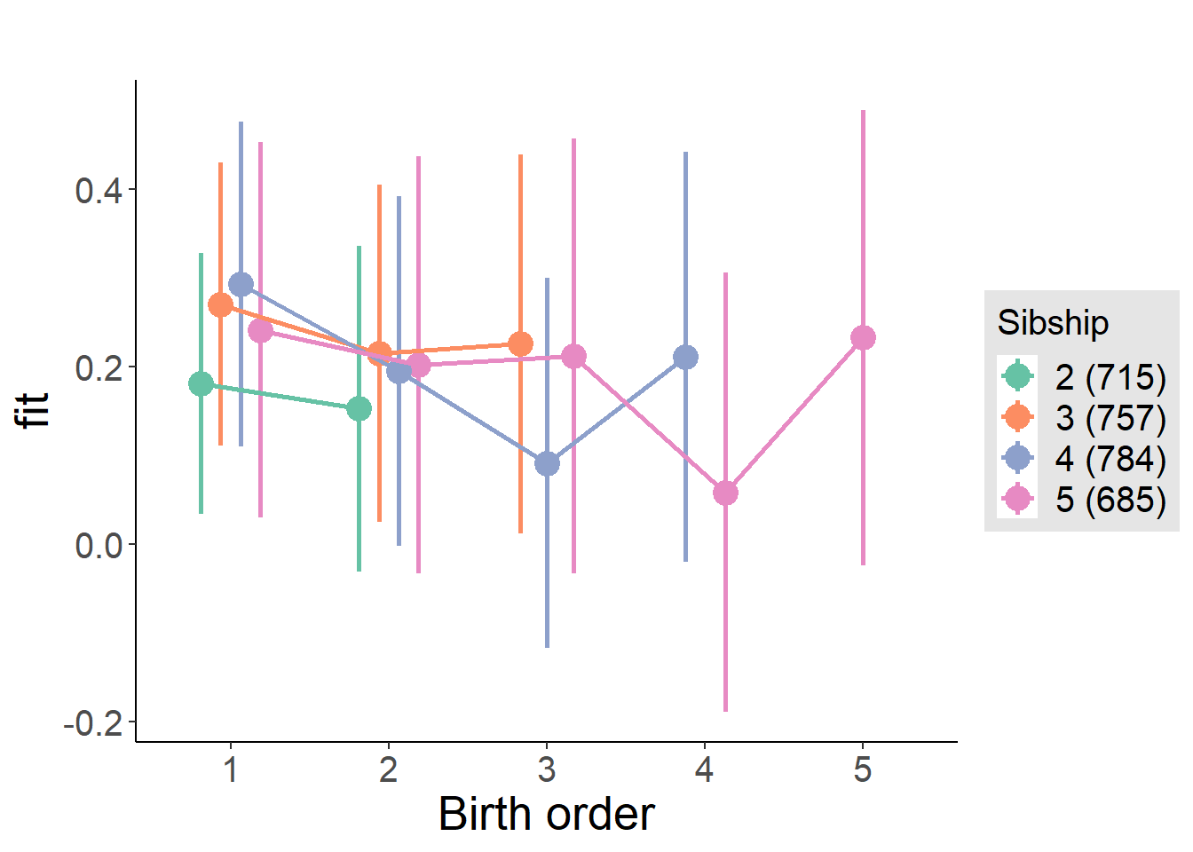
Model Comparison
###### Model 1 - Model 2
anova(m1_covariates_only, m2_birthorder_linear, m3_birthorder_nonlinear, m4_interaction)## refitting model(s) with ML (instead of REML)| Df | AIC | BIC | logLik | deviance | Chisq | Chi Df | Pr(>Chisq) |
|---|---|---|---|---|---|---|---|
| 10 | 8206 | 8266 | -4093 | 8186 | NA | NA | NA |
| 11 | 8206 | 8271 | -4092 | 8184 | 2.534 | 1 | 0.1114 |
| 14 | 8209 | 8293 | -4091 | 8181 | 2.169 | 3 | 0.5382 |
| 20 | 8218 | 8337 | -4089 | 8178 | 3.899 | 6 | 0.6904 |
Maternal birth order
outcome_uterus_m1 <- update(m2_birthorder_linear, data = birthorder %>%
mutate(sibling_count = sibling_count_uterus_alive_factor,
birth_order_nonlinear = birthorder_uterus_alive_factor,
birth_order = birthorder_uterus_alive,
count_birth_order = count_birthorder_uterus_alive) %>%
filter(sibling_count != "1"))
compare_models_markdown(outcome_uterus_m1)Basic Model
Model Summary
m1_covariates_only <- update(m2_birthorder_linear, formula = . ~ . - birth_order)
tidy(m1_covariates_only, conf.int = T, conf.level = 0.995)| effect | group | term | estimate | std.error | statistic | df | p.value | conf.low | conf.high |
|---|---|---|---|---|---|---|---|---|---|
| fixed | NA | (Intercept) | -5.041 | 1.155 | -4.366 | 1866 | 0.00001337 | -8.283 | -1.8 |
| fixed | NA | poly(age, 3, raw = TRUE)1 | 0.4195 | 0.1269 | 3.305 | 1867 | 0.0009669 | 0.06323 | 0.7757 |
| fixed | NA | poly(age, 3, raw = TRUE)2 | -0.01122 | 0.004483 | -2.504 | 1867 | 0.01238 | -0.02381 | 0.00136 |
| fixed | NA | poly(age, 3, raw = TRUE)3 | 0.0001023 | 0.00005091 | 2.009 | 1866 | 0.04464 | -0.00004061 | 0.0002452 |
| fixed | NA | male | 0.1532 | 0.04694 | 3.265 | 1882 | 0.001115 | 0.02149 | 0.285 |
| fixed | NA | sibling_count3 | 0.03305 | 0.06361 | 0.5196 | 1480 | 0.6034 | -0.1455 | 0.2116 |
| fixed | NA | sibling_count4 | -0.0503 | 0.06578 | -0.7647 | 1362 | 0.4446 | -0.2349 | 0.1343 |
| fixed | NA | sibling_count5 | -0.1586 | 0.0749 | -2.118 | 1260 | 0.03439 | -0.3689 | 0.05163 |
| ran_pars | mother_pidlink | sd__(Intercept) | 0.2671 | NA | NA | NA | NA | NA | NA |
| ran_pars | Residual | sd__Observation | 0.9643 | NA | NA | NA | NA | NA | NA |
Coefficient Plot
plot(allEffects(m1_covariates_only, confidence.level = 0.995))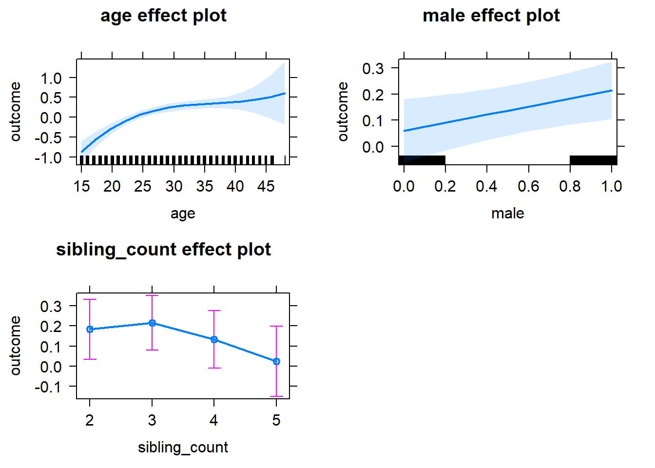
Add Birth Order Linear
Model Summary
tidy(m2_birthorder_linear, conf.int = T, conf.level = 0.995)| effect | group | term | estimate | std.error | statistic | df | p.value | conf.low | conf.high |
|---|---|---|---|---|---|---|---|---|---|
| fixed | NA | (Intercept) | -5.044 | 1.155 | -4.366 | 1865 | 0.00001335 | -8.286 | -1.801 |
| fixed | NA | birth_order | 0.002807 | 0.02376 | 0.1181 | 1812 | 0.906 | -0.0639 | 0.06951 |
| fixed | NA | poly(age, 3, raw = TRUE)1 | 0.4194 | 0.1269 | 3.304 | 1866 | 0.0009706 | 0.06311 | 0.7758 |
| fixed | NA | poly(age, 3, raw = TRUE)2 | -0.01123 | 0.004484 | -2.504 | 1866 | 0.01237 | -0.02381 | 0.00136 |
| fixed | NA | poly(age, 3, raw = TRUE)3 | 0.0001024 | 0.00005093 | 2.011 | 1865 | 0.0445 | -0.00004056 | 0.0002454 |
| fixed | NA | male | 0.1532 | 0.04695 | 3.263 | 1881 | 0.001124 | 0.02139 | 0.285 |
| fixed | NA | sibling_count3 | 0.03178 | 0.06455 | 0.4923 | 1501 | 0.6226 | -0.1494 | 0.213 |
| fixed | NA | sibling_count4 | -0.0532 | 0.07025 | -0.7573 | 1468 | 0.449 | -0.2504 | 0.144 |
| fixed | NA | sibling_count5 | -0.1636 | 0.08589 | -1.904 | 1456 | 0.05704 | -0.4047 | 0.07752 |
| ran_pars | mother_pidlink | sd__(Intercept) | 0.2675 | NA | NA | NA | NA | NA | NA |
| ran_pars | Residual | sd__Observation | 0.9645 | NA | NA | NA | NA | NA | NA |
Coefficient Plot
plot_birthorder2(m2_birthorder_linear, separate = FALSE)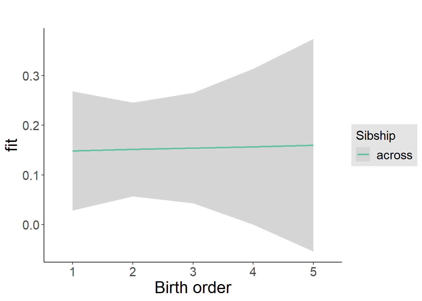
Add Birth Order Factor
Model Summary
m3_birthorder_nonlinear = update(m1_covariates_only, formula = . ~ . + birth_order_nonlinear)
tidy(m3_birthorder_nonlinear, conf.int = T, conf.level = 0.995)| effect | group | term | estimate | std.error | statistic | df | p.value | conf.low | conf.high |
|---|---|---|---|---|---|---|---|---|---|
| fixed | NA | (Intercept) | -5.015 | 1.156 | -4.339 | 1861 | 0.00001505 | -8.26 | -1.771 |
| fixed | NA | poly(age, 3, raw = TRUE)1 | 0.4156 | 0.127 | 3.271 | 1862 | 0.00109 | 0.05898 | 0.7722 |
| fixed | NA | poly(age, 3, raw = TRUE)2 | -0.0111 | 0.004487 | -2.475 | 1863 | 0.01342 | -0.0237 | 0.00149 |
| fixed | NA | poly(age, 3, raw = TRUE)3 | 0.0001011 | 0.00005096 | 1.985 | 1861 | 0.0473 | -0.00004189 | 0.0002442 |
| fixed | NA | male | 0.1517 | 0.04695 | 3.231 | 1878 | 0.001253 | 0.01993 | 0.2835 |
| fixed | NA | sibling_count3 | 0.02238 | 0.06548 | 0.3418 | 1543 | 0.7326 | -0.1614 | 0.2062 |
| fixed | NA | sibling_count4 | -0.07671 | 0.07122 | -1.077 | 1515 | 0.2816 | -0.2766 | 0.1232 |
| fixed | NA | sibling_count5 | -0.1312 | 0.08736 | -1.502 | 1475 | 0.1332 | -0.3765 | 0.114 |
| fixed | NA | birth_order_nonlinear2 | 0.04756 | 0.05625 | 0.8455 | 1599 | 0.3979 | -0.1103 | 0.2055 |
| fixed | NA | birth_order_nonlinear3 | 0.05026 | 0.06967 | 0.7213 | 1682 | 0.4708 | -0.1453 | 0.2458 |
| fixed | NA | birth_order_nonlinear4 | 0.08852 | 0.09217 | 0.9604 | 1728 | 0.337 | -0.1702 | 0.3473 |
| fixed | NA | birth_order_nonlinear5 | -0.2357 | 0.1428 | -1.651 | 1775 | 0.09891 | -0.6365 | 0.165 |
| ran_pars | mother_pidlink | sd__(Intercept) | 0.2674 | NA | NA | NA | NA | NA | NA |
| ran_pars | Residual | sd__Observation | 0.9638 | NA | NA | NA | NA | NA | NA |
Coefficient Plot
plot_birthorder(m3_birthorder_nonlinear, separate = FALSE)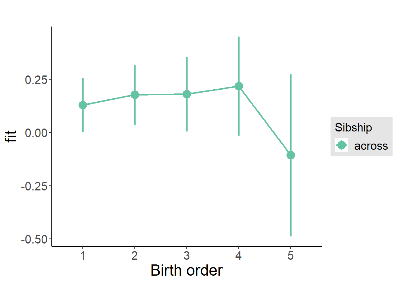
Add Interaction
Model Summary
m4_interaction = update(m3_birthorder_nonlinear, formula = . ~ . - birth_order_nonlinear - sibling_count + count_birth_order)
tidy(m4_interaction, conf.int = T, conf.level = 0.995)| effect | group | term | estimate | std.error | statistic | df | p.value | conf.low | conf.high |
|---|---|---|---|---|---|---|---|---|---|
| fixed | NA | (Intercept) | -4.943 | 1.158 | -4.267 | 1854 | 0.00002083 | -8.195 | -1.691 |
| fixed | NA | poly(age, 3, raw = TRUE)1 | 0.4062 | 0.1275 | 3.187 | 1855 | 0.001462 | 0.04841 | 0.764 |
| fixed | NA | poly(age, 3, raw = TRUE)2 | -0.01073 | 0.004503 | -2.383 | 1855 | 0.01726 | -0.02337 | 0.001909 |
| fixed | NA | poly(age, 3, raw = TRUE)3 | 0.0000965 | 0.00005115 | 1.887 | 1854 | 0.05938 | -0.00004709 | 0.0002401 |
| fixed | NA | male | 0.1496 | 0.04705 | 3.181 | 1872 | 0.001493 | 0.01758 | 0.2817 |
| fixed | NA | count_birth_order2/2 | 0.05432 | 0.1003 | 0.5414 | 1632 | 0.5883 | -0.2273 | 0.3359 |
| fixed | NA | count_birth_order1/3 | 0.009103 | 0.08335 | 0.1092 | 1875 | 0.913 | -0.2249 | 0.2431 |
| fixed | NA | count_birth_order2/3 | 0.1111 | 0.09459 | 1.175 | 1874 | 0.2403 | -0.1544 | 0.3766 |
| fixed | NA | count_birth_order3/3 | 0.05426 | 0.1041 | 0.5212 | 1871 | 0.6023 | -0.238 | 0.3465 |
| fixed | NA | count_birth_order1/4 | -0.09662 | 0.09804 | -0.9855 | 1875 | 0.3245 | -0.3718 | 0.1786 |
| fixed | NA | count_birth_order2/4 | -0.06522 | 0.1012 | -0.6443 | 1874 | 0.5194 | -0.3494 | 0.2189 |
| fixed | NA | count_birth_order3/4 | 0.04807 | 0.1069 | 0.4499 | 1870 | 0.6528 | -0.2519 | 0.348 |
| fixed | NA | count_birth_order4/4 | 0.01509 | 0.1141 | 0.1323 | 1869 | 0.8948 | -0.3051 | 0.3352 |
| fixed | NA | count_birth_order1/5 | -0.01062 | 0.1323 | -0.08023 | 1875 | 0.9361 | -0.3821 | 0.3609 |
| fixed | NA | count_birth_order2/5 | -0.1219 | 0.154 | -0.7916 | 1867 | 0.4287 | -0.5542 | 0.3104 |
| fixed | NA | count_birth_order3/5 | -0.1815 | 0.1388 | -1.307 | 1872 | 0.1914 | -0.5712 | 0.2083 |
| fixed | NA | count_birth_order4/5 | -0.04254 | 0.131 | -0.3247 | 1869 | 0.7455 | -0.4103 | 0.3252 |
| fixed | NA | count_birth_order5/5 | -0.366 | 0.135 | -2.711 | 1870 | 0.006768 | -0.745 | 0.01296 |
| ran_pars | mother_pidlink | sd__(Intercept) | 0.2669 | NA | NA | NA | NA | NA | NA |
| ran_pars | Residual | sd__Observation | 0.9647 | NA | NA | NA | NA | NA | NA |
Coefficient Plot
plot_birthorder(m4_interaction)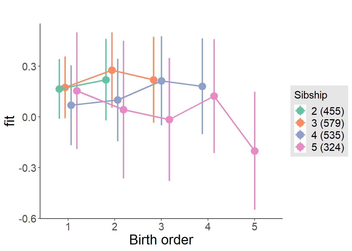
Model Comparison
###### Model 1 - Model 2
anova(m1_covariates_only, m2_birthorder_linear, m3_birthorder_nonlinear, m4_interaction)## refitting model(s) with ML (instead of REML)| Df | AIC | BIC | logLik | deviance | Chisq | Chi Df | Pr(>Chisq) |
|---|---|---|---|---|---|---|---|
| 10 | 5384 | 5440 | -2682 | 5364 | NA | NA | NA |
| 11 | 5386 | 5447 | -2682 | 5364 | 0.01322 | 1 | 0.9085 |
| 14 | 5386 | 5464 | -2679 | 5358 | 5.689 | 3 | 0.1278 |
| 20 | 5395 | 5506 | -2678 | 5355 | 3.141 | 6 | 0.7909 |
Maternal pregnancy order
outcome_preg_m1 <- update(m2_birthorder_linear, data = birthorder %>%
mutate(sibling_count = sibling_count_uterus_preg_factor,
birth_order_nonlinear = birthorder_uterus_preg_factor,
birth_order = birthorder_uterus_preg,
count_birth_order = count_birthorder_uterus_preg
) %>%
filter(sibling_count != "1"))
compare_models_markdown(outcome_preg_m1)Basic Model
Model Summary
m1_covariates_only <- update(m2_birthorder_linear, formula = . ~ . - birth_order)
tidy(m1_covariates_only, conf.int = T, conf.level = 0.995)| effect | group | term | estimate | std.error | statistic | df | p.value | conf.low | conf.high |
|---|---|---|---|---|---|---|---|---|---|
| fixed | NA | (Intercept) | -5.112 | 1.176 | -4.348 | 1727 | 0.00001457 | -8.412 | -1.811 |
| fixed | NA | poly(age, 3, raw = TRUE)1 | 0.4281 | 0.1293 | 3.311 | 1729 | 0.0009505 | 0.06511 | 0.7912 |
| fixed | NA | poly(age, 3, raw = TRUE)2 | -0.0115 | 0.00457 | -2.517 | 1730 | 0.01192 | -0.02433 | 0.001325 |
| fixed | NA | poly(age, 3, raw = TRUE)3 | 0.0001046 | 0.00005193 | 2.015 | 1729 | 0.04409 | -0.00004114 | 0.0002504 |
| fixed | NA | male | 0.1328 | 0.04798 | 2.767 | 1733 | 0.005719 | -0.001924 | 0.2675 |
| fixed | NA | sibling_count3 | 0.03107 | 0.06907 | 0.4499 | 1395 | 0.6529 | -0.1628 | 0.225 |
| fixed | NA | sibling_count4 | 0.01523 | 0.07028 | 0.2167 | 1317 | 0.8285 | -0.182 | 0.2125 |
| fixed | NA | sibling_count5 | -0.1259 | 0.07391 | -1.703 | 1224 | 0.08874 | -0.3334 | 0.08156 |
| ran_pars | mother_pidlink | sd__(Intercept) | 0.309 | NA | NA | NA | NA | NA | NA |
| ran_pars | Residual | sd__Observation | 0.9334 | NA | NA | NA | NA | NA | NA |
Coefficient Plot
plot(allEffects(m1_covariates_only, confidence.level = 0.995))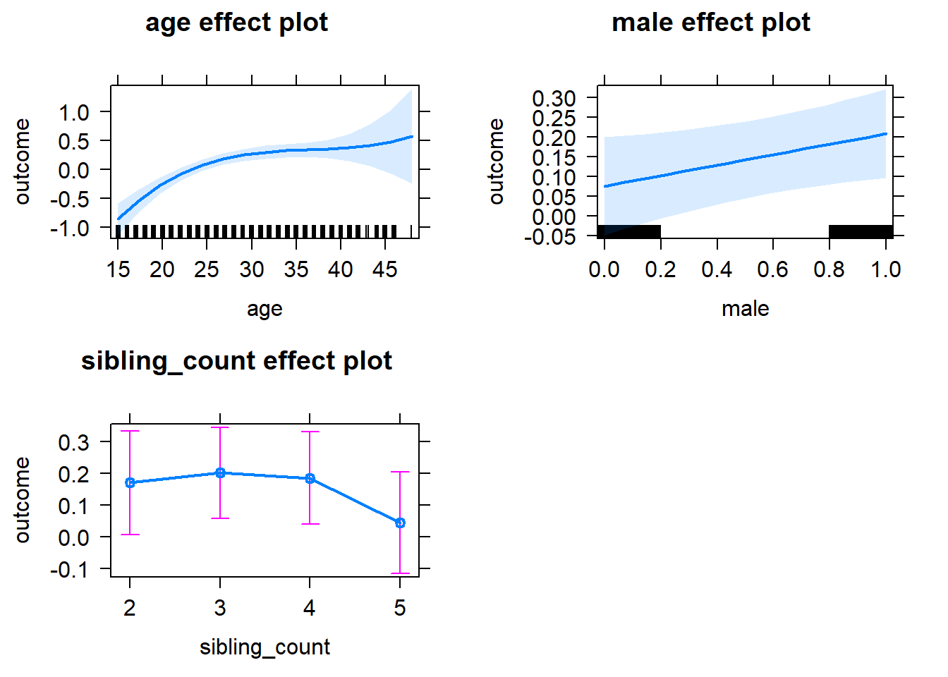
Add Birth Order Linear
Model Summary
tidy(m2_birthorder_linear, conf.int = T, conf.level = 0.995)| effect | group | term | estimate | std.error | statistic | df | p.value | conf.low | conf.high |
|---|---|---|---|---|---|---|---|---|---|
| fixed | NA | (Intercept) | -5.117 | 1.177 | -4.349 | 1726 | 0.00001448 | -8.42 | -1.814 |
| fixed | NA | birth_order | 0.003539 | 0.02331 | 0.1518 | 1689 | 0.8794 | -0.06191 | 0.06898 |
| fixed | NA | poly(age, 3, raw = TRUE)1 | 0.4283 | 0.1294 | 3.311 | 1728 | 0.0009504 | 0.06514 | 0.7914 |
| fixed | NA | poly(age, 3, raw = TRUE)2 | -0.01151 | 0.004572 | -2.518 | 1729 | 0.01188 | -0.02435 | 0.00132 |
| fixed | NA | poly(age, 3, raw = TRUE)3 | 0.0001048 | 0.00005195 | 2.017 | 1728 | 0.04382 | -0.00004103 | 0.0002506 |
| fixed | NA | male | 0.1328 | 0.048 | 2.766 | 1732 | 0.005737 | -0.001974 | 0.2675 |
| fixed | NA | sibling_count3 | 0.02938 | 0.06998 | 0.4199 | 1409 | 0.6746 | -0.167 | 0.2258 |
| fixed | NA | sibling_count4 | 0.01171 | 0.07402 | 0.1582 | 1382 | 0.8743 | -0.1961 | 0.2195 |
| fixed | NA | sibling_count5 | -0.1316 | 0.083 | -1.586 | 1374 | 0.113 | -0.3646 | 0.1014 |
| ran_pars | mother_pidlink | sd__(Intercept) | 0.3094 | NA | NA | NA | NA | NA | NA |
| ran_pars | Residual | sd__Observation | 0.9335 | NA | NA | NA | NA | NA | NA |
Coefficient Plot
plot_birthorder2(m2_birthorder_linear, separate = FALSE)
Add Birth Order Factor
Model Summary
m3_birthorder_nonlinear = update(m1_covariates_only, formula = . ~ . + birth_order_nonlinear)
tidy(m3_birthorder_nonlinear, conf.int = T, conf.level = 0.995)| effect | group | term | estimate | std.error | statistic | df | p.value | conf.low | conf.high |
|---|---|---|---|---|---|---|---|---|---|
| fixed | NA | (Intercept) | -5.143 | 1.177 | -4.37 | 1722 | 0.00001315 | -8.446 | -1.84 |
| fixed | NA | poly(age, 3, raw = TRUE)1 | 0.4305 | 0.1295 | 3.325 | 1724 | 0.0009028 | 0.06705 | 0.7939 |
| fixed | NA | poly(age, 3, raw = TRUE)2 | -0.01159 | 0.004575 | -2.534 | 1725 | 0.01137 | -0.02443 | 0.001249 |
| fixed | NA | poly(age, 3, raw = TRUE)3 | 0.0001057 | 0.00005198 | 2.034 | 1724 | 0.04212 | -0.00004019 | 0.0002516 |
| fixed | NA | male | 0.1319 | 0.04798 | 2.75 | 1730 | 0.006025 | -0.002745 | 0.2666 |
| fixed | NA | sibling_count3 | 0.01588 | 0.07092 | 0.224 | 1440 | 0.8228 | -0.1832 | 0.2149 |
| fixed | NA | sibling_count4 | -0.02047 | 0.07489 | -0.2733 | 1417 | 0.7847 | -0.2307 | 0.1898 |
| fixed | NA | sibling_count5 | -0.1114 | 0.08345 | -1.335 | 1379 | 0.1821 | -0.3457 | 0.1228 |
| fixed | NA | birth_order_nonlinear2 | 0.04053 | 0.05715 | 0.7092 | 1460 | 0.4783 | -0.1199 | 0.201 |
| fixed | NA | birth_order_nonlinear3 | 0.06525 | 0.07116 | 0.917 | 1567 | 0.3593 | -0.1345 | 0.265 |
| fixed | NA | birth_order_nonlinear4 | 0.1259 | 0.09257 | 1.36 | 1575 | 0.1739 | -0.1339 | 0.3858 |
| fixed | NA | birth_order_nonlinear5 | -0.2428 | 0.1317 | -1.844 | 1620 | 0.06542 | -0.6124 | 0.1269 |
| ran_pars | mother_pidlink | sd__(Intercept) | 0.3112 | NA | NA | NA | NA | NA | NA |
| ran_pars | Residual | sd__Observation | 0.9315 | NA | NA | NA | NA | NA | NA |
Coefficient Plot
plot_birthorder(m3_birthorder_nonlinear, separate = FALSE)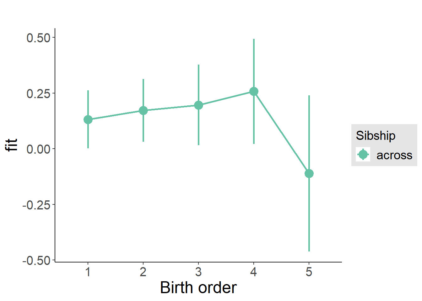
Add Interaction
Model Summary
m4_interaction = update(m3_birthorder_nonlinear, formula = . ~ . - birth_order_nonlinear - sibling_count + count_birth_order)
tidy(m4_interaction, conf.int = T, conf.level = 0.995)| effect | group | term | estimate | std.error | statistic | df | p.value | conf.low | conf.high |
|---|---|---|---|---|---|---|---|---|---|
| fixed | NA | (Intercept) | -5.113 | 1.182 | -4.324 | 1715 | 0.00001621 | -8.432 | -1.794 |
| fixed | NA | poly(age, 3, raw = TRUE)1 | 0.4261 | 0.1302 | 3.273 | 1717 | 0.001083 | 0.06072 | 0.7915 |
| fixed | NA | poly(age, 3, raw = TRUE)2 | -0.0114 | 0.0046 | -2.479 | 1718 | 0.01329 | -0.02431 | 0.001511 |
| fixed | NA | poly(age, 3, raw = TRUE)3 | 0.0001032 | 0.00005227 | 1.975 | 1717 | 0.04847 | -0.00004351 | 0.0002499 |
| fixed | NA | male | 0.1304 | 0.04817 | 2.707 | 1723 | 0.00685 | -0.004802 | 0.2656 |
| fixed | NA | count_birth_order2/2 | 0.03909 | 0.111 | 0.3523 | 1544 | 0.7247 | -0.2724 | 0.3505 |
| fixed | NA | count_birth_order1/3 | -0.01466 | 0.09025 | -0.1624 | 1730 | 0.871 | -0.268 | 0.2387 |
| fixed | NA | count_birth_order2/3 | 0.1055 | 0.1001 | 1.053 | 1731 | 0.2924 | -0.1756 | 0.3866 |
| fixed | NA | count_birth_order3/3 | 0.07192 | 0.1119 | 0.6426 | 1727 | 0.5206 | -0.2422 | 0.3861 |
| fixed | NA | count_birth_order1/4 | -0.002117 | 0.1018 | -0.0208 | 1731 | 0.9834 | -0.2878 | 0.2836 |
| fixed | NA | count_birth_order2/4 | 0.0178 | 0.1023 | 0.1739 | 1730 | 0.862 | -0.2695 | 0.3051 |
| fixed | NA | count_birth_order3/4 | 0.02894 | 0.1154 | 0.2509 | 1724 | 0.8019 | -0.2949 | 0.3528 |
| fixed | NA | count_birth_order4/4 | 0.08847 | 0.1225 | 0.7223 | 1719 | 0.4702 | -0.2554 | 0.4323 |
| fixed | NA | count_birth_order1/5 | -0.07416 | 0.1184 | -0.6263 | 1731 | 0.5312 | -0.4065 | 0.2582 |
| fixed | NA | count_birth_order2/5 | -0.1721 | 0.1301 | -1.323 | 1722 | 0.186 | -0.5372 | 0.193 |
| fixed | NA | count_birth_order3/5 | -0.01529 | 0.1297 | -0.1179 | 1722 | 0.9062 | -0.3795 | 0.3489 |
| fixed | NA | count_birth_order4/5 | 0.03177 | 0.1305 | 0.2434 | 1714 | 0.8077 | -0.3347 | 0.3982 |
| fixed | NA | count_birth_order5/5 | -0.3552 | 0.1301 | -2.731 | 1720 | 0.006384 | -0.7204 | 0.009928 |
| ran_pars | mother_pidlink | sd__(Intercept) | 0.315 | NA | NA | NA | NA | NA | NA |
| ran_pars | Residual | sd__Observation | 0.9316 | NA | NA | NA | NA | NA | NA |
Coefficient Plot
plot_birthorder(m4_interaction)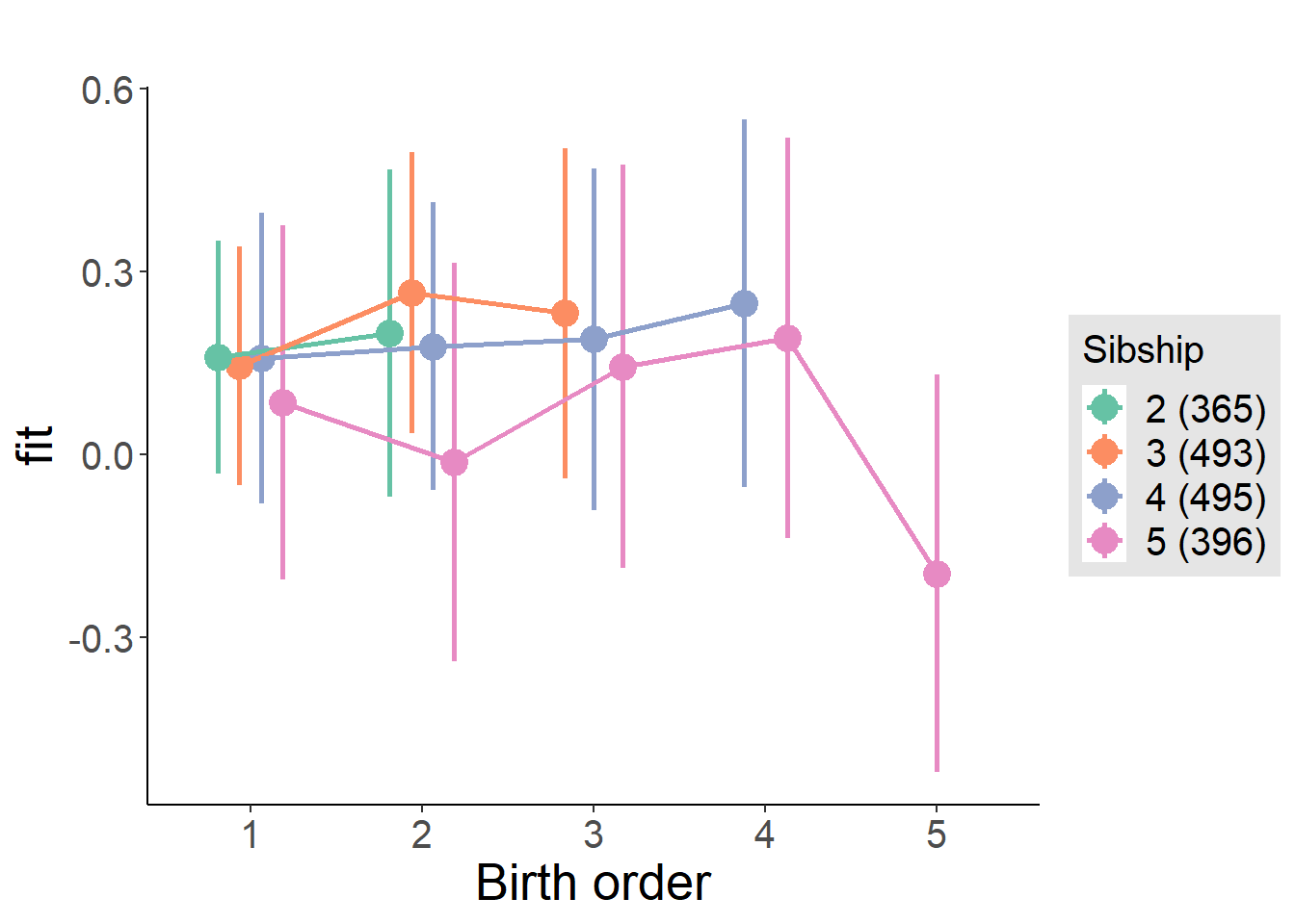
Model Comparison
###### Model 1 - Model 2
anova(m1_covariates_only, m2_birthorder_linear, m3_birthorder_nonlinear, m4_interaction)## refitting model(s) with ML (instead of REML)| Df | AIC | BIC | logLik | deviance | Chisq | Chi Df | Pr(>Chisq) |
|---|---|---|---|---|---|---|---|
| 10 | 4912 | 4967 | -2446 | 4892 | NA | NA | NA |
| 11 | 4914 | 4974 | -2446 | 4892 | 0.02233 | 1 | 0.8812 |
| 14 | 4912 | 4989 | -2442 | 4884 | 7.814 | 3 | 0.05001 |
| 20 | 4922 | 5032 | -2441 | 4882 | 1.813 | 6 | 0.936 |
Parental full sibling order
outcome_parental_m1 <- update(m2_birthorder_linear, data = birthorder %>%
mutate(sibling_count = sibling_count_genes_factor,
birth_order_nonlinear = birthorder_genes_factor,
birth_order = birthorder_genes,
count_birth_order = count_birthorder_genes
) %>%
filter(sibling_count != "1"))
compare_models_markdown(outcome_parental_m1)Basic Model
Model Summary
m1_covariates_only <- update(m2_birthorder_linear, formula = . ~ . - birth_order)
tidy(m1_covariates_only, conf.int = T, conf.level = 0.995)| effect | group | term | estimate | std.error | statistic | df | p.value | conf.low | conf.high |
|---|---|---|---|---|---|---|---|---|---|
| fixed | NA | (Intercept) | -4.797 | 1.195 | -4.015 | 1857 | 0.00006192 | -8.151 | -1.443 |
| fixed | NA | poly(age, 3, raw = TRUE)1 | 0.3884 | 0.1314 | 2.957 | 1858 | 0.003147 | 0.01968 | 0.7571 |
| fixed | NA | poly(age, 3, raw = TRUE)2 | -0.01 | 0.004639 | -2.156 | 1859 | 0.03123 | -0.02302 | 0.003022 |
| fixed | NA | poly(age, 3, raw = TRUE)3 | 0.00008709 | 0.00005269 | 1.653 | 1858 | 0.09853 | -0.00006082 | 0.000235 |
| fixed | NA | male | 0.1802 | 0.04862 | 3.706 | 1868 | 0.000217 | 0.04369 | 0.3167 |
| fixed | NA | sibling_count3 | -0.005082 | 0.06501 | -0.07817 | 1474 | 0.9377 | -0.1876 | 0.1774 |
| fixed | NA | sibling_count4 | -0.1041 | 0.06798 | -1.531 | 1348 | 0.1261 | -0.2949 | 0.08676 |
| fixed | NA | sibling_count5 | -0.1696 | 0.07966 | -2.129 | 1207 | 0.03345 | -0.3932 | 0.05401 |
| ran_pars | mother_pidlink | sd__(Intercept) | 0.3022 | NA | NA | NA | NA | NA | NA |
| ran_pars | Residual | sd__Observation | 0.9897 | NA | NA | NA | NA | NA | NA |
Coefficient Plot
plot(allEffects(m1_covariates_only, confidence.level = 0.995))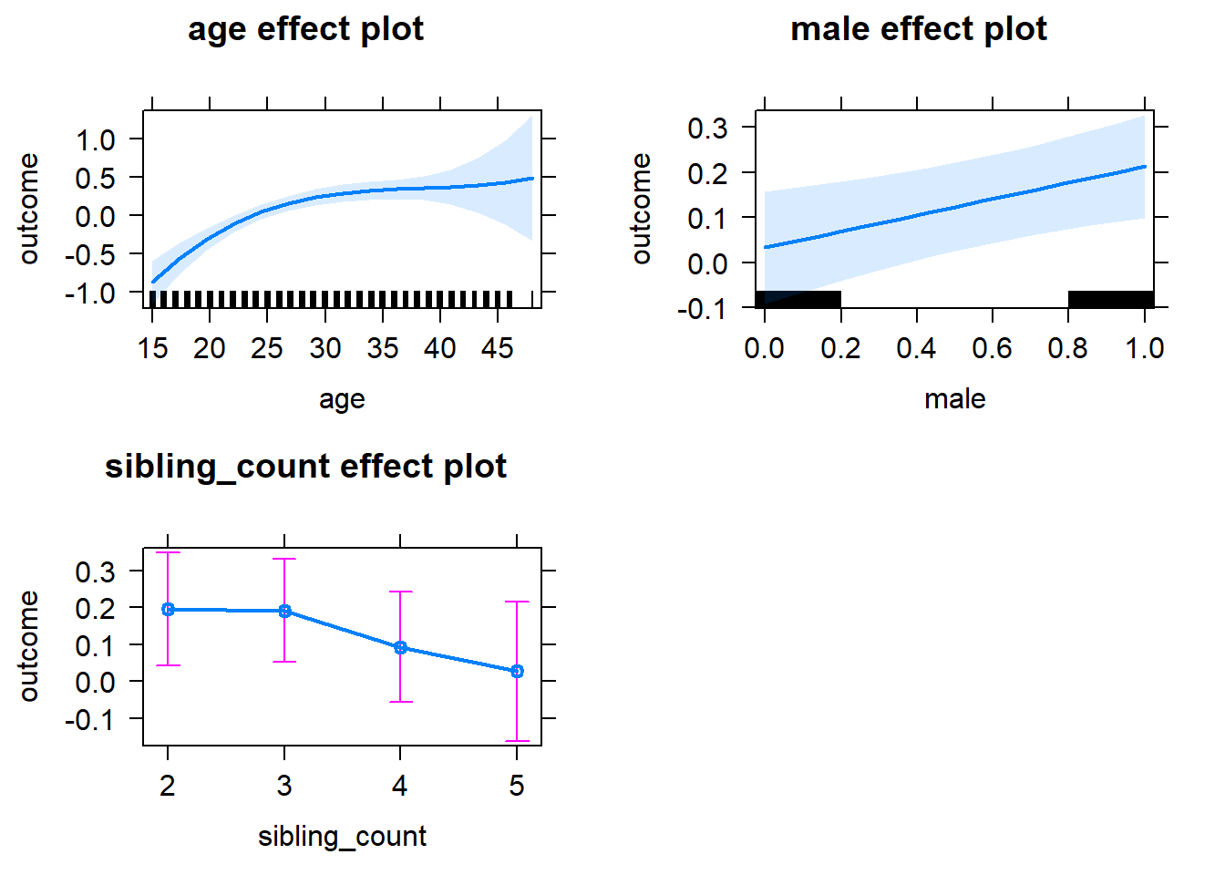
Add Birth Order Linear
Model Summary
tidy(m2_birthorder_linear, conf.int = T, conf.level = 0.995)| effect | group | term | estimate | std.error | statistic | df | p.value | conf.low | conf.high |
|---|---|---|---|---|---|---|---|---|---|
| fixed | NA | (Intercept) | -4.799 | 1.195 | -4.015 | 1856 | 0.00006175 | -8.154 | -1.444 |
| fixed | NA | birth_order | 0.003711 | 0.02502 | 0.1483 | 1780 | 0.8821 | -0.06653 | 0.07395 |
| fixed | NA | poly(age, 3, raw = TRUE)1 | 0.3883 | 0.1314 | 2.955 | 1857 | 0.003165 | 0.01945 | 0.7571 |
| fixed | NA | poly(age, 3, raw = TRUE)2 | -0.01 | 0.004641 | -2.156 | 1858 | 0.03124 | -0.02303 | 0.003023 |
| fixed | NA | poly(age, 3, raw = TRUE)3 | 0.00008721 | 0.00005271 | 1.654 | 1857 | 0.09821 | -0.00006076 | 0.0002352 |
| fixed | NA | male | 0.1801 | 0.04864 | 3.703 | 1867 | 0.0002196 | 0.04356 | 0.3166 |
| fixed | NA | sibling_count3 | -0.006814 | 0.06607 | -0.1031 | 1493 | 0.9179 | -0.1923 | 0.1787 |
| fixed | NA | sibling_count4 | -0.1078 | 0.07259 | -1.485 | 1460 | 0.1377 | -0.3116 | 0.09593 |
| fixed | NA | sibling_count5 | -0.176 | 0.09046 | -1.945 | 1401 | 0.05195 | -0.4299 | 0.07796 |
| ran_pars | mother_pidlink | sd__(Intercept) | 0.3026 | NA | NA | NA | NA | NA | NA |
| ran_pars | Residual | sd__Observation | 0.9898 | NA | NA | NA | NA | NA | NA |
Coefficient Plot
plot_birthorder2(m2_birthorder_linear, separate = FALSE)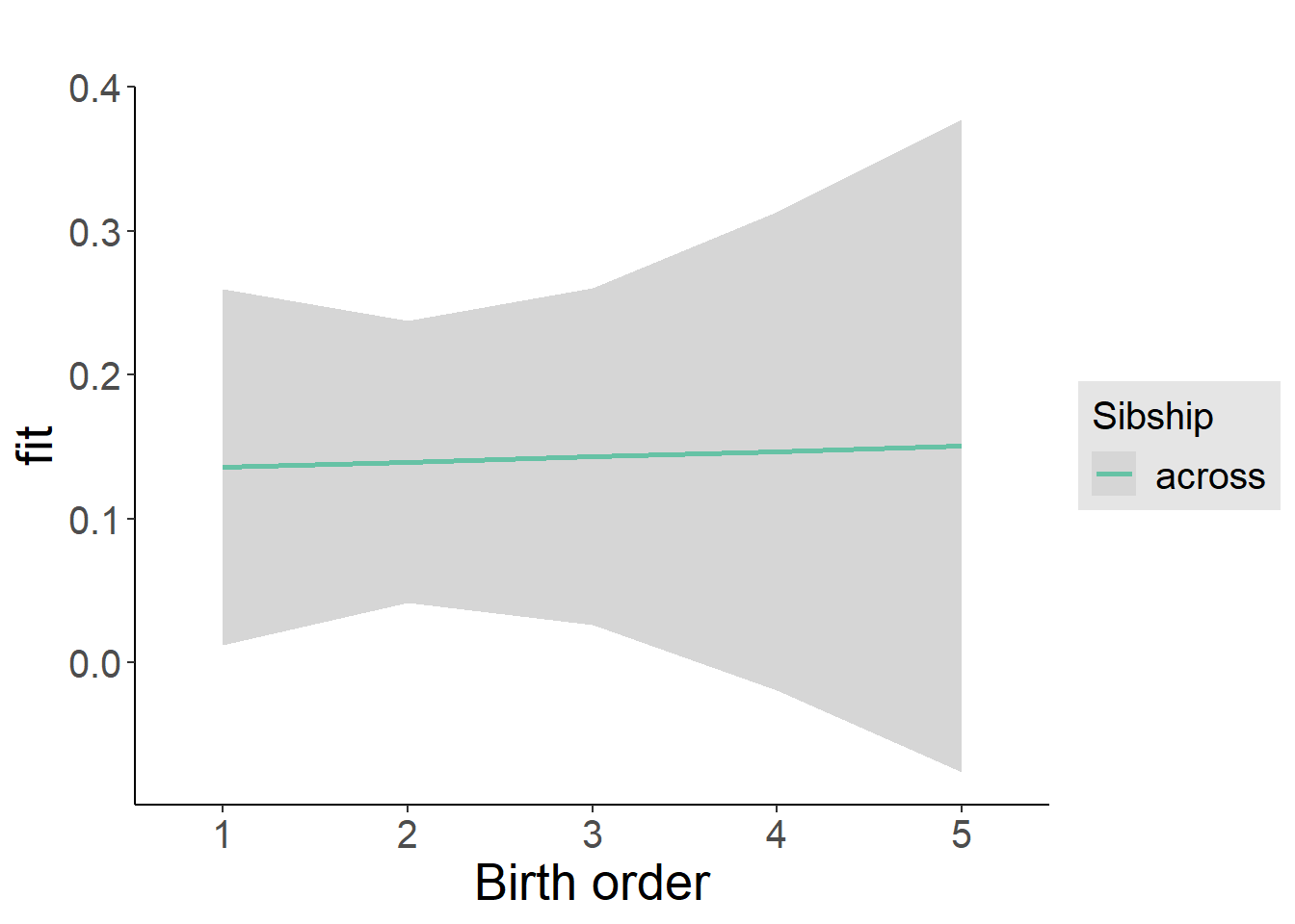
Add Birth Order Factor
Model Summary
m3_birthorder_nonlinear = update(m1_covariates_only, formula = . ~ . + birth_order_nonlinear)
tidy(m3_birthorder_nonlinear, conf.int = T, conf.level = 0.995)| effect | group | term | estimate | std.error | statistic | df | p.value | conf.low | conf.high |
|---|---|---|---|---|---|---|---|---|---|
| fixed | NA | (Intercept) | -4.85 | 1.197 | -4.052 | 1853 | 0.00005293 | -8.211 | -1.49 |
| fixed | NA | poly(age, 3, raw = TRUE)1 | 0.3941 | 0.1316 | 2.994 | 1855 | 0.002793 | 0.02457 | 0.7636 |
| fixed | NA | poly(age, 3, raw = TRUE)2 | -0.01022 | 0.004649 | -2.198 | 1855 | 0.02804 | -0.02327 | 0.002829 |
| fixed | NA | poly(age, 3, raw = TRUE)3 | 0.00008963 | 0.0000528 | 1.698 | 1854 | 0.08975 | -0.00005857 | 0.0002378 |
| fixed | NA | male | 0.1809 | 0.04871 | 3.714 | 1865 | 0.0002099 | 0.04419 | 0.3177 |
| fixed | NA | sibling_count3 | -0.02507 | 0.06715 | -0.3734 | 1533 | 0.7089 | -0.2136 | 0.1634 |
| fixed | NA | sibling_count4 | -0.1232 | 0.0736 | -1.674 | 1505 | 0.09434 | -0.3298 | 0.08339 |
| fixed | NA | sibling_count5 | -0.1493 | 0.09234 | -1.617 | 1430 | 0.106 | -0.4085 | 0.1099 |
| fixed | NA | birth_order_nonlinear2 | 0.02734 | 0.05778 | 0.4731 | 1572 | 0.6362 | -0.1349 | 0.1895 |
| fixed | NA | birth_order_nonlinear3 | 0.08955 | 0.07184 | 1.247 | 1664 | 0.2127 | -0.1121 | 0.2912 |
| fixed | NA | birth_order_nonlinear4 | 0.001777 | 0.0986 | 0.01802 | 1679 | 0.9856 | -0.275 | 0.2785 |
| fixed | NA | birth_order_nonlinear5 | -0.1624 | 0.1567 | -1.037 | 1746 | 0.3 | -0.6022 | 0.2774 |
| ran_pars | mother_pidlink | sd__(Intercept) | 0.3069 | NA | NA | NA | NA | NA | NA |
| ran_pars | Residual | sd__Observation | 0.9885 | NA | NA | NA | NA | NA | NA |
Coefficient Plot
plot_birthorder(m3_birthorder_nonlinear, separate = FALSE)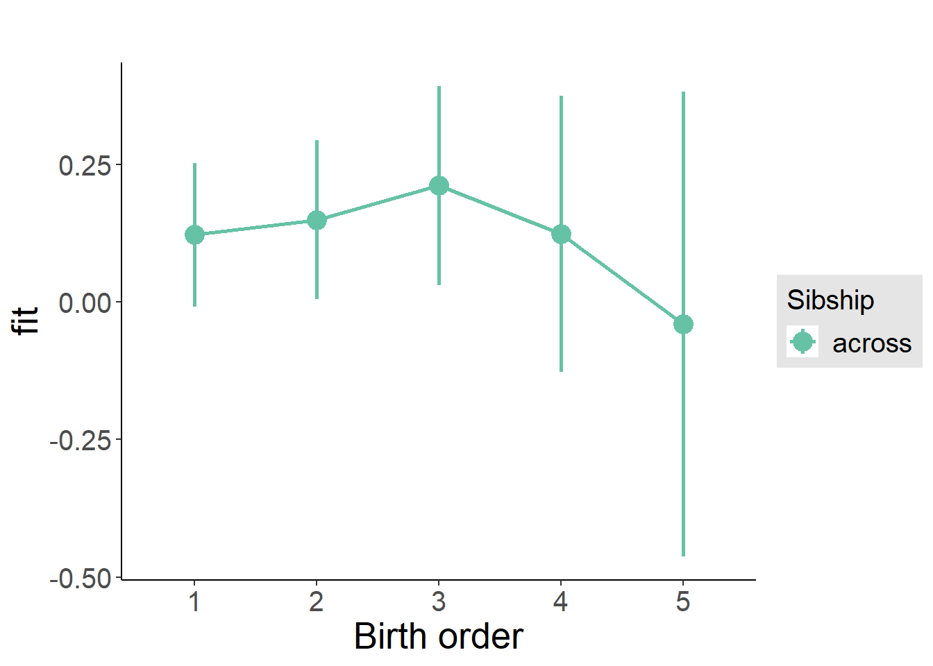
Add Interaction
Model Summary
m4_interaction = update(m3_birthorder_nonlinear, formula = . ~ . - birth_order_nonlinear - sibling_count + count_birth_order)
tidy(m4_interaction, conf.int = T, conf.level = 0.995)| effect | group | term | estimate | std.error | statistic | df | p.value | conf.low | conf.high |
|---|---|---|---|---|---|---|---|---|---|
| fixed | NA | (Intercept) | -4.789 | 1.2 | -3.992 | 1846 | 0.00006804 | -8.156 | -1.422 |
| fixed | NA | poly(age, 3, raw = TRUE)1 | 0.3862 | 0.1321 | 2.924 | 1847 | 0.003497 | 0.01545 | 0.7569 |
| fixed | NA | poly(age, 3, raw = TRUE)2 | -0.00988 | 0.004665 | -2.118 | 1848 | 0.03431 | -0.02298 | 0.003214 |
| fixed | NA | poly(age, 3, raw = TRUE)3 | 0.00008515 | 0.00005299 | 1.607 | 1847 | 0.1082 | -0.00006359 | 0.0002339 |
| fixed | NA | male | 0.1773 | 0.04881 | 3.632 | 1859 | 0.0002891 | 0.04025 | 0.3143 |
| fixed | NA | count_birth_order2/2 | 0.0157 | 0.1012 | 0.1552 | 1595 | 0.8767 | -0.2683 | 0.2997 |
| fixed | NA | count_birth_order1/3 | -0.06288 | 0.08534 | -0.7368 | 1863 | 0.4613 | -0.3024 | 0.1767 |
| fixed | NA | count_birth_order2/3 | 0.07646 | 0.09722 | 0.7865 | 1862 | 0.4317 | -0.1964 | 0.3494 |
| fixed | NA | count_birth_order3/3 | 0.0301 | 0.1049 | 0.2869 | 1858 | 0.7742 | -0.2643 | 0.3245 |
| fixed | NA | count_birth_order1/4 | -0.1383 | 0.102 | -1.357 | 1864 | 0.175 | -0.4245 | 0.1479 |
| fixed | NA | count_birth_order2/4 | -0.1647 | 0.1043 | -1.579 | 1862 | 0.1144 | -0.4576 | 0.1281 |
| fixed | NA | count_birth_order3/4 | 0.02634 | 0.1104 | 0.2387 | 1859 | 0.8114 | -0.2834 | 0.3361 |
| fixed | NA | count_birth_order4/4 | -0.0892 | 0.1208 | -0.7385 | 1853 | 0.4603 | -0.4283 | 0.2499 |
| fixed | NA | count_birth_order1/5 | -0.002734 | 0.1398 | -0.01955 | 1864 | 0.9844 | -0.3953 | 0.3898 |
| fixed | NA | count_birth_order2/5 | -0.1924 | 0.162 | -1.188 | 1855 | 0.2349 | -0.6471 | 0.2622 |
| fixed | NA | count_birth_order3/5 | -0.129 | 0.1505 | -0.8576 | 1858 | 0.3912 | -0.5514 | 0.2933 |
| fixed | NA | count_birth_order4/5 | -0.2067 | 0.1427 | -1.448 | 1853 | 0.1477 | -0.6074 | 0.1939 |
| fixed | NA | count_birth_order5/5 | -0.3173 | 0.1478 | -2.147 | 1856 | 0.03195 | -0.7321 | 0.09761 |
| ran_pars | mother_pidlink | sd__(Intercept) | 0.3045 | NA | NA | NA | NA | NA | NA |
| ran_pars | Residual | sd__Observation | 0.9896 | NA | NA | NA | NA | NA | NA |
Coefficient Plot
plot_birthorder(m4_interaction)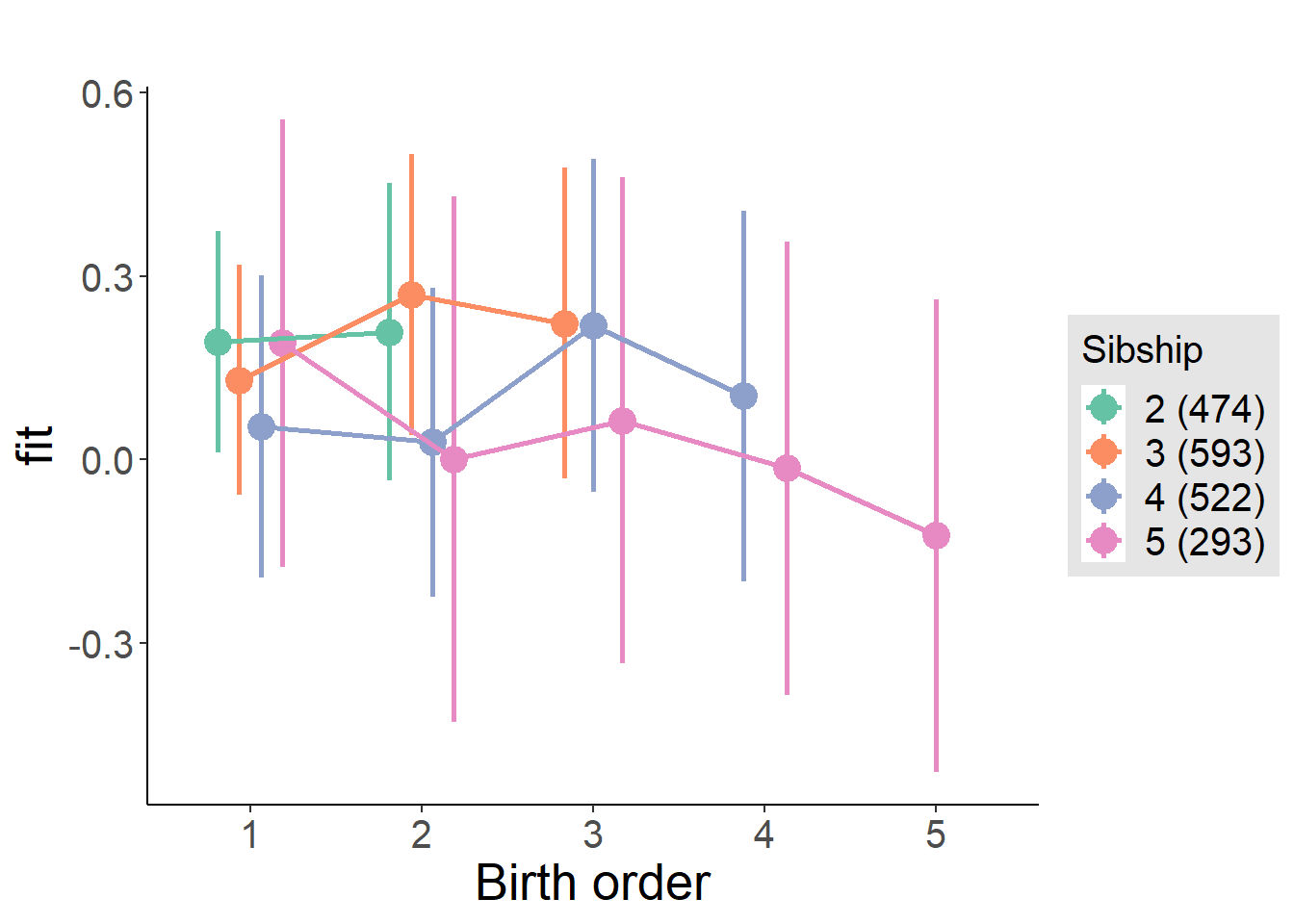
Model Comparison
###### Model 1 - Model 2
anova(m1_covariates_only, m2_birthorder_linear, m3_birthorder_nonlinear, m4_interaction)## refitting model(s) with ML (instead of REML)| Df | AIC | BIC | logLik | deviance | Chisq | Chi Df | Pr(>Chisq) |
|---|---|---|---|---|---|---|---|
| 10 | 5478 | 5534 | -2729 | 5458 | NA | NA | NA |
| 11 | 5480 | 5541 | -2729 | 5458 | 0.02131 | 1 | 0.8839 |
| 14 | 5483 | 5560 | -2727 | 5455 | 3.279 | 3 | 0.3506 |
| 20 | 5490 | 5601 | -2725 | 5450 | 4.76 | 6 | 0.575 |
Compare birth order specifications
library(coefplot)
multiplot(outcome_naive_m1, outcome_preg_m1, outcome_uterus_m1, outcome_parental_m1, dodgeHeight = 0.6,
intercept = FALSE)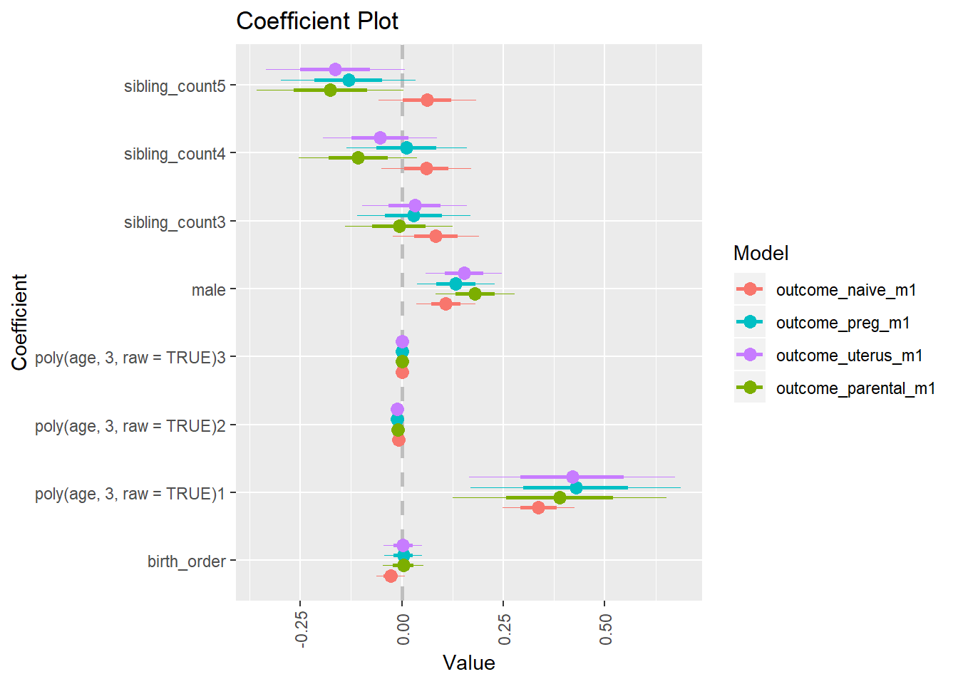
Self-Employment - non standardized
birthorder <- birthorder %>% mutate(outcome = Self_employed)
model = lmer(outcome ~ birth_order + poly(age, 3, raw = TRUE) + male + sibling_count + (1 | mother_pidlink),
data = birthorder)
compare_birthorder_specs(model)Naive birth order
outcome_naive_m1 <- update(m2_birthorder_linear, data = birthorder %>%
mutate(sibling_count = sibling_count_naive_factor,
birth_order_nonlinear = birthorder_naive_factor,
birth_order = birthorder_naive,
count_birth_order = count_birthorder_naive) %>%
filter(sibling_count != "1"))
compare_models_markdown(outcome_naive_m1)Basic Model
Model Summary
m1_covariates_only <- update(m2_birthorder_linear, formula = . ~ . - birth_order)
tidy(m1_covariates_only, conf.int = T, conf.level = 0.995)| effect | group | term | estimate | std.error | statistic | df | p.value | conf.low | conf.high |
|---|---|---|---|---|---|---|---|---|---|
| fixed | NA | (Intercept) | -0.1206 | 0.1226 | -0.9834 | 4493 | 0.3255 | -0.4647 | 0.2236 |
| fixed | NA | poly(age, 3, raw = TRUE)1 | 0.012 | 0.01094 | 1.097 | 4392 | 0.2727 | -0.01871 | 0.04271 |
| fixed | NA | poly(age, 3, raw = TRUE)2 | 0.0001217 | 0.0003039 | 0.4005 | 4271 | 0.6888 | -0.0007313 | 0.0009746 |
| fixed | NA | poly(age, 3, raw = TRUE)3 | -0.000002423 | 0.000002658 | -0.9116 | 4161 | 0.3621 | -0.000009883 | 0.000005038 |
| fixed | NA | male | -0.007402 | 0.0124 | -0.5968 | 4755 | 0.5507 | -0.04222 | 0.02741 |
| fixed | NA | sibling_count3 | -0.02237 | 0.01799 | -1.243 | 3513 | 0.2138 | -0.07286 | 0.02813 |
| fixed | NA | sibling_count4 | -0.01961 | 0.0182 | -1.078 | 3307 | 0.2812 | -0.07069 | 0.03147 |
| fixed | NA | sibling_count5 | -0.009391 | 0.019 | -0.4943 | 3086 | 0.6211 | -0.06272 | 0.04394 |
| ran_pars | mother_pidlink | sd__(Intercept) | 0.1564 | NA | NA | NA | NA | NA | NA |
| ran_pars | Residual | sd__Observation | 0.3995 | NA | NA | NA | NA | NA | NA |
Coefficient Plot
plot(allEffects(m1_covariates_only, confidence.level = 0.995))
Add Birth Order Linear
Model Summary
tidy(m2_birthorder_linear, conf.int = T, conf.level = 0.995)| effect | group | term | estimate | std.error | statistic | df | p.value | conf.low | conf.high |
|---|---|---|---|---|---|---|---|---|---|
| fixed | NA | (Intercept) | -0.1194 | 0.1226 | -0.9736 | 4493 | 0.3303 | -0.4635 | 0.2248 |
| fixed | NA | birth_order | 0.006512 | 0.006069 | 1.073 | 4244 | 0.2833 | -0.01052 | 0.02355 |
| fixed | NA | poly(age, 3, raw = TRUE)1 | 0.01103 | 0.01098 | 1.005 | 4392 | 0.3151 | -0.01978 | 0.04184 |
| fixed | NA | poly(age, 3, raw = TRUE)2 | 0.0001463 | 0.0003047 | 0.4803 | 4262 | 0.6311 | -0.000709 | 0.001002 |
| fixed | NA | poly(age, 3, raw = TRUE)3 | -0.000002589 | 0.000002662 | -0.9726 | 4153 | 0.3308 | -0.00001006 | 0.000004884 |
| fixed | NA | male | -0.007341 | 0.0124 | -0.5919 | 4754 | 0.554 | -0.04215 | 0.02747 |
| fixed | NA | sibling_count3 | -0.02483 | 0.01813 | -1.369 | 3598 | 0.171 | -0.07573 | 0.02607 |
| fixed | NA | sibling_count4 | -0.02483 | 0.01884 | -1.318 | 3649 | 0.1874 | -0.07771 | 0.02804 |
| fixed | NA | sibling_count5 | -0.01774 | 0.02053 | -0.8642 | 3771 | 0.3875 | -0.07537 | 0.03989 |
| ran_pars | mother_pidlink | sd__(Intercept) | 0.1564 | NA | NA | NA | NA | NA | NA |
| ran_pars | Residual | sd__Observation | 0.3995 | NA | NA | NA | NA | NA | NA |
Coefficient Plot
plot_birthorder2(m2_birthorder_linear, separate = FALSE)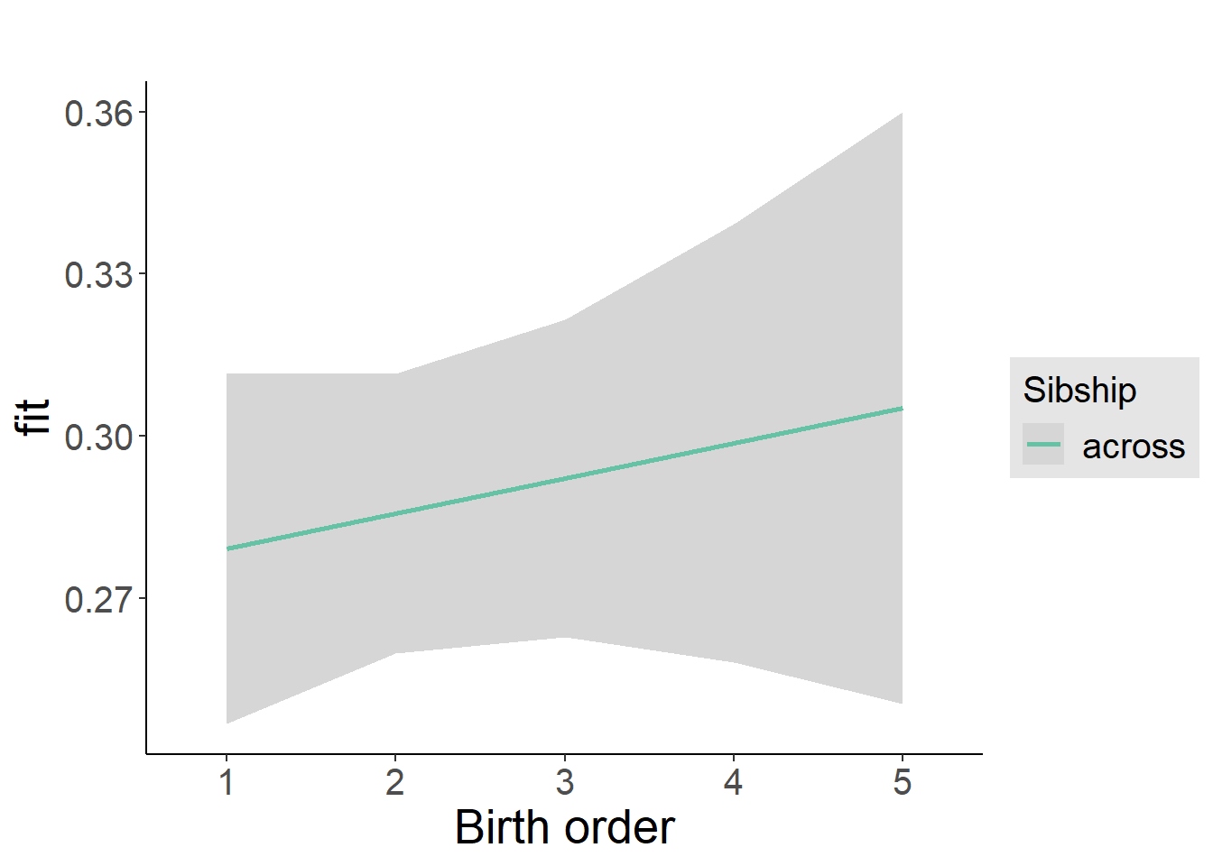
Add Birth Order Factor
Model Summary
m3_birthorder_nonlinear = update(m1_covariates_only, formula = . ~ . + birth_order_nonlinear)
tidy(m3_birthorder_nonlinear, conf.int = T, conf.level = 0.995)| effect | group | term | estimate | std.error | statistic | df | p.value | conf.low | conf.high |
|---|---|---|---|---|---|---|---|---|---|
| fixed | NA | (Intercept) | -0.1273 | 0.1229 | -1.036 | 4498 | 0.3001 | -0.4723 | 0.2176 |
| fixed | NA | poly(age, 3, raw = TRUE)1 | 0.01147 | 0.01097 | 1.046 | 4389 | 0.2958 | -0.01933 | 0.04228 |
| fixed | NA | poly(age, 3, raw = TRUE)2 | 0.0001204 | 0.0003047 | 0.3952 | 4256 | 0.6927 | -0.0007349 | 0.0009757 |
| fixed | NA | poly(age, 3, raw = TRUE)3 | -0.000002249 | 0.000002663 | -0.8444 | 4140 | 0.3985 | -0.000009726 | 0.000005227 |
| fixed | NA | male | -0.00794 | 0.0124 | -0.6405 | 4750 | 0.5219 | -0.04274 | 0.02686 |
| fixed | NA | sibling_count3 | -0.02604 | 0.01843 | -1.413 | 3746 | 0.1577 | -0.07777 | 0.02568 |
| fixed | NA | sibling_count4 | -0.02219 | 0.01914 | -1.159 | 3802 | 0.2466 | -0.07593 | 0.03155 |
| fixed | NA | sibling_count5 | -0.01043 | 0.02071 | -0.5038 | 3865 | 0.6144 | -0.06857 | 0.04771 |
| fixed | NA | birth_order_nonlinear2 | 0.04641 | 0.01462 | 3.175 | 4168 | 0.001509 | 0.00538 | 0.08745 |
| fixed | NA | birth_order_nonlinear3 | 0.02766 | 0.01859 | 1.488 | 4101 | 0.1369 | -0.02453 | 0.07985 |
| fixed | NA | birth_order_nonlinear4 | 0.01196 | 0.02414 | 0.4955 | 4060 | 0.6203 | -0.0558 | 0.07972 |
| fixed | NA | birth_order_nonlinear5 | 0.009981 | 0.03487 | 0.2862 | 4070 | 0.7747 | -0.08791 | 0.1079 |
| ran_pars | mother_pidlink | sd__(Intercept) | 0.1568 | NA | NA | NA | NA | NA | NA |
| ran_pars | Residual | sd__Observation | 0.3991 | NA | NA | NA | NA | NA | NA |
Coefficient Plot
plot_birthorder(m3_birthorder_nonlinear, separate = FALSE)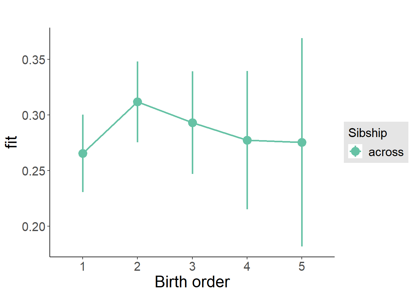
Add Interaction
Model Summary
m4_interaction = update(m3_birthorder_nonlinear, formula = . ~ . - birth_order_nonlinear - sibling_count + count_birth_order)
tidy(m4_interaction, conf.int = T, conf.level = 0.995)| effect | group | term | estimate | std.error | statistic | df | p.value | conf.low | conf.high |
|---|---|---|---|---|---|---|---|---|---|
| fixed | NA | (Intercept) | -0.1265 | 0.123 | -1.028 | 4502 | 0.3039 | -0.4718 | 0.2189 |
| fixed | NA | poly(age, 3, raw = TRUE)1 | 0.01062 | 0.01098 | 0.9672 | 4386 | 0.3335 | -0.0202 | 0.04144 |
| fixed | NA | poly(age, 3, raw = TRUE)2 | 0.0001361 | 0.0003048 | 0.4465 | 4253 | 0.6553 | -0.0007194 | 0.0009916 |
| fixed | NA | poly(age, 3, raw = TRUE)3 | -0.000002308 | 0.000002664 | -0.8666 | 4137 | 0.3862 | -0.000009785 | 0.000005168 |
| fixed | NA | male | -0.008281 | 0.0124 | -0.6679 | 4743 | 0.5042 | -0.04309 | 0.02652 |
| fixed | NA | count_birth_order2/2 | 0.07691 | 0.02482 | 3.098 | 4123 | 0.001961 | 0.007225 | 0.1466 |
| fixed | NA | count_birth_order1/3 | -0.02403 | 0.02407 | -0.9984 | 4793 | 0.3182 | -0.09159 | 0.04353 |
| fixed | NA | count_birth_order2/3 | 0.03415 | 0.02669 | 1.28 | 4804 | 0.2008 | -0.04077 | 0.1091 |
| fixed | NA | count_birth_order3/3 | 0.02757 | 0.02937 | 0.9389 | 4806 | 0.3478 | -0.05486 | 0.11 |
| fixed | NA | count_birth_order1/4 | 0.01578 | 0.02638 | 0.5979 | 4804 | 0.5499 | -0.05829 | 0.08984 |
| fixed | NA | count_birth_order2/4 | 0.006164 | 0.0283 | 0.2178 | 4806 | 0.8276 | -0.07327 | 0.0856 |
| fixed | NA | count_birth_order3/4 | -0.003886 | 0.03019 | -0.1287 | 4804 | 0.8976 | -0.08862 | 0.08085 |
| fixed | NA | count_birth_order4/4 | 0.02151 | 0.03211 | 0.67 | 4803 | 0.5029 | -0.06863 | 0.1117 |
| fixed | NA | count_birth_order1/5 | 0.01111 | 0.02995 | 0.3709 | 4804 | 0.7107 | -0.07297 | 0.09518 |
| fixed | NA | count_birth_order2/5 | 0.0492 | 0.03179 | 1.547 | 4801 | 0.1218 | -0.04004 | 0.1384 |
| fixed | NA | count_birth_order3/5 | 0.03627 | 0.03346 | 1.084 | 4796 | 0.2785 | -0.05767 | 0.1302 |
| fixed | NA | count_birth_order4/5 | -0.01264 | 0.03519 | -0.359 | 4775 | 0.7196 | -0.1114 | 0.08615 |
| fixed | NA | count_birth_order5/5 | 0.01104 | 0.03522 | 0.3136 | 4791 | 0.7539 | -0.08782 | 0.1099 |
| ran_pars | mother_pidlink | sd__(Intercept) | 0.1569 | NA | NA | NA | NA | NA | NA |
| ran_pars | Residual | sd__Observation | 0.399 | NA | NA | NA | NA | NA | NA |
Coefficient Plot
plot_birthorder(m4_interaction)
Model Comparison
###### Model 1 - Model 2
anova(m1_covariates_only, m2_birthorder_linear, m3_birthorder_nonlinear, m4_interaction)## refitting model(s) with ML (instead of REML)| Df | AIC | BIC | logLik | deviance | Chisq | Chi Df | Pr(>Chisq) |
|---|---|---|---|---|---|---|---|
| 10 | 5504 | 5569 | -2742 | 5484 | NA | NA | NA |
| 11 | 5505 | 5576 | -2741 | 5483 | 1.154 | 1 | 0.2828 |
| 14 | 5501 | 5592 | -2737 | 5473 | 9.456 | 3 | 0.0238 |
| 20 | 5506 | 5635 | -2733 | 5466 | 7.697 | 6 | 0.2612 |
Maternal birth order
outcome_uterus_m1 <- update(m2_birthorder_linear, data = birthorder %>%
mutate(sibling_count = sibling_count_uterus_alive_factor,
birth_order_nonlinear = birthorder_uterus_alive_factor,
birth_order = birthorder_uterus_alive,
count_birth_order = count_birthorder_uterus_alive) %>%
filter(sibling_count != "1"))
compare_models_markdown(outcome_uterus_m1)Basic Model
Model Summary
m1_covariates_only <- update(m2_birthorder_linear, formula = . ~ . - birth_order)
tidy(m1_covariates_only, conf.int = T, conf.level = 0.995)| effect | group | term | estimate | std.error | statistic | df | p.value | conf.low | conf.high |
|---|---|---|---|---|---|---|---|---|---|
| fixed | NA | (Intercept) | 1.112 | 0.3187 | 3.489 | 2759 | 0.000492 | 0.2174 | 2.007 |
| fixed | NA | poly(age, 3, raw = TRUE)1 | -0.1214 | 0.03531 | -3.439 | 2760 | 0.0005935 | -0.2205 | -0.0223 |
| fixed | NA | poly(age, 3, raw = TRUE)2 | 0.004639 | 0.001252 | 3.705 | 2760 | 0.0002156 | 0.001124 | 0.008154 |
| fixed | NA | poly(age, 3, raw = TRUE)3 | -0.00005136 | 0.00001422 | -3.611 | 2760 | 0.00031 | -0.00009129 | -0.00001144 |
| fixed | NA | male | -0.04191 | 0.0149 | -2.813 | 2721 | 0.004946 | -0.08373 | -0.00008659 |
| fixed | NA | sibling_count3 | 0.01673 | 0.02117 | 0.7903 | 2217 | 0.4294 | -0.04269 | 0.07615 |
| fixed | NA | sibling_count4 | -0.02678 | 0.022 | -1.217 | 2081 | 0.2236 | -0.08852 | 0.03497 |
| fixed | NA | sibling_count5 | 0.04089 | 0.02453 | 1.667 | 1873 | 0.09571 | -0.02797 | 0.1098 |
| ran_pars | mother_pidlink | sd__(Intercept) | 0.157 | NA | NA | NA | NA | NA | NA |
| ran_pars | Residual | sd__Observation | 0.3561 | NA | NA | NA | NA | NA | NA |
Coefficient Plot
plot(allEffects(m1_covariates_only, confidence.level = 0.995))
Add Birth Order Linear
Model Summary
tidy(m2_birthorder_linear, conf.int = T, conf.level = 0.995)| effect | group | term | estimate | std.error | statistic | df | p.value | conf.low | conf.high |
|---|---|---|---|---|---|---|---|---|---|
| fixed | NA | (Intercept) | 1.113 | 0.3188 | 3.49 | 2758 | 0.0004908 | 0.2177 | 2.008 |
| fixed | NA | birth_order | -0.001112 | 0.007469 | -0.1489 | 2589 | 0.8816 | -0.02208 | 0.01985 |
| fixed | NA | poly(age, 3, raw = TRUE)1 | -0.1213 | 0.03532 | -3.435 | 2758 | 0.0006009 | -0.2205 | -0.02218 |
| fixed | NA | poly(age, 3, raw = TRUE)2 | 0.004638 | 0.001252 | 3.703 | 2759 | 0.0002169 | 0.001123 | 0.008153 |
| fixed | NA | poly(age, 3, raw = TRUE)3 | -0.00005138 | 0.00001423 | -3.612 | 2759 | 0.0003095 | -0.00009131 | -0.00001145 |
| fixed | NA | male | -0.04191 | 0.0149 | -2.812 | 2720 | 0.004953 | -0.08374 | -0.00007972 |
| fixed | NA | sibling_count3 | 0.01727 | 0.02148 | 0.8039 | 2246 | 0.4215 | -0.04303 | 0.07756 |
| fixed | NA | sibling_count4 | -0.02562 | 0.02332 | -1.099 | 2194 | 0.2719 | -0.09108 | 0.03983 |
| fixed | NA | sibling_count5 | 0.04282 | 0.02776 | 1.543 | 2169 | 0.123 | -0.03509 | 0.1207 |
| ran_pars | mother_pidlink | sd__(Intercept) | 0.1571 | NA | NA | NA | NA | NA | NA |
| ran_pars | Residual | sd__Observation | 0.3561 | NA | NA | NA | NA | NA | NA |
Coefficient Plot
plot_birthorder2(m2_birthorder_linear, separate = FALSE)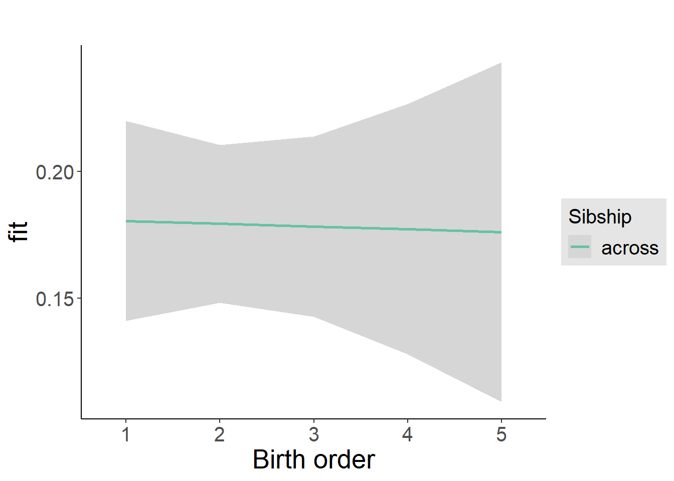
Add Birth Order Factor
Model Summary
m3_birthorder_nonlinear = update(m1_covariates_only, formula = . ~ . + birth_order_nonlinear)
tidy(m3_birthorder_nonlinear, conf.int = T, conf.level = 0.995)| effect | group | term | estimate | std.error | statistic | df | p.value | conf.low | conf.high |
|---|---|---|---|---|---|---|---|---|---|
| fixed | NA | (Intercept) | 1.113 | 0.3195 | 3.483 | 2755 | 0.0005044 | 0.2159 | 2.01 |
| fixed | NA | poly(age, 3, raw = TRUE)1 | -0.1218 | 0.03539 | -3.443 | 2755 | 0.0005845 | -0.2212 | -0.0225 |
| fixed | NA | poly(age, 3, raw = TRUE)2 | 0.004652 | 0.001255 | 3.708 | 2756 | 0.0002134 | 0.00113 | 0.008175 |
| fixed | NA | poly(age, 3, raw = TRUE)3 | -0.00005151 | 0.00001425 | -3.614 | 2756 | 0.0003066 | -0.00009151 | -0.0000115 |
| fixed | NA | male | -0.04216 | 0.01491 | -2.827 | 2718 | 0.004737 | -0.08402 | -0.0002938 |
| fixed | NA | sibling_count3 | 0.01836 | 0.02179 | 0.8423 | 2302 | 0.3997 | -0.04282 | 0.07954 |
| fixed | NA | sibling_count4 | -0.02705 | 0.02361 | -1.146 | 2246 | 0.252 | -0.09334 | 0.03923 |
| fixed | NA | sibling_count5 | 0.0469 | 0.0281 | 1.669 | 2210 | 0.09523 | -0.03198 | 0.1258 |
| fixed | NA | birth_order_nonlinear2 | 0.01228 | 0.01776 | 0.691 | 2336 | 0.4896 | -0.03759 | 0.06214 |
| fixed | NA | birth_order_nonlinear3 | -0.005867 | 0.02171 | -0.2702 | 2396 | 0.787 | -0.06681 | 0.05508 |
| fixed | NA | birth_order_nonlinear4 | 0.01255 | 0.02887 | 0.4346 | 2459 | 0.6639 | -0.06849 | 0.09359 |
| fixed | NA | birth_order_nonlinear5 | -0.02938 | 0.0443 | -0.6631 | 2389 | 0.5073 | -0.1537 | 0.09498 |
| ran_pars | mother_pidlink | sd__(Intercept) | 0.1575 | NA | NA | NA | NA | NA | NA |
| ran_pars | Residual | sd__Observation | 0.3561 | NA | NA | NA | NA | NA | NA |
Coefficient Plot
plot_birthorder(m3_birthorder_nonlinear, separate = FALSE)
Add Interaction
Model Summary
m4_interaction = update(m3_birthorder_nonlinear, formula = . ~ . - birth_order_nonlinear - sibling_count + count_birth_order)
tidy(m4_interaction, conf.int = T, conf.level = 0.995)| effect | group | term | estimate | std.error | statistic | df | p.value | conf.low | conf.high |
|---|---|---|---|---|---|---|---|---|---|
| fixed | NA | (Intercept) | 1.101 | 0.3199 | 3.443 | 2749 | 0.0005833 | 0.2035 | 1.999 |
| fixed | NA | poly(age, 3, raw = TRUE)1 | -0.122 | 0.03542 | -3.443 | 2749 | 0.0005832 | -0.2214 | -0.02254 |
| fixed | NA | poly(age, 3, raw = TRUE)2 | 0.004655 | 0.001256 | 3.706 | 2750 | 0.0002145 | 0.001129 | 0.008181 |
| fixed | NA | poly(age, 3, raw = TRUE)3 | -0.00005152 | 0.00001427 | -3.611 | 2750 | 0.0003104 | -0.00009157 | -0.00001147 |
| fixed | NA | male | -0.04244 | 0.01494 | -2.841 | 2712 | 0.00453 | -0.08437 | -0.0005087 |
| fixed | NA | count_birth_order2/2 | 0.0532 | 0.03229 | 1.648 | 2406 | 0.09955 | -0.03743 | 0.1438 |
| fixed | NA | count_birth_order1/3 | 0.04188 | 0.02754 | 1.52 | 2745 | 0.1285 | -0.03544 | 0.1192 |
| fixed | NA | count_birth_order2/3 | 0.03959 | 0.03056 | 1.296 | 2750 | 0.1952 | -0.04619 | 0.1254 |
| fixed | NA | count_birth_order3/3 | 0.01101 | 0.03305 | 0.3331 | 2746 | 0.7391 | -0.08175 | 0.1038 |
| fixed | NA | count_birth_order1/4 | -0.006186 | 0.03172 | -0.195 | 2749 | 0.8454 | -0.09522 | 0.08285 |
| fixed | NA | count_birth_order2/4 | -0.02662 | 0.03329 | -0.7996 | 2747 | 0.424 | -0.1201 | 0.06682 |
| fixed | NA | count_birth_order3/4 | -0.01179 | 0.03488 | -0.338 | 2737 | 0.7354 | -0.1097 | 0.08611 |
| fixed | NA | count_birth_order4/4 | 0.01099 | 0.03695 | 0.2973 | 2735 | 0.7663 | -0.09273 | 0.1147 |
| fixed | NA | count_birth_order1/5 | 0.05724 | 0.04167 | 1.374 | 2747 | 0.1697 | -0.05974 | 0.1742 |
| fixed | NA | count_birth_order2/5 | 0.07863 | 0.04519 | 1.74 | 2719 | 0.08198 | -0.04822 | 0.2055 |
| fixed | NA | count_birth_order3/5 | 0.06885 | 0.0423 | 1.628 | 2724 | 0.1037 | -0.04988 | 0.1876 |
| fixed | NA | count_birth_order4/5 | 0.05676 | 0.0411 | 1.381 | 2722 | 0.1674 | -0.0586 | 0.1721 |
| fixed | NA | count_birth_order5/5 | 0.03067 | 0.04307 | 0.712 | 2715 | 0.4765 | -0.09024 | 0.1516 |
| ran_pars | mother_pidlink | sd__(Intercept) | 0.1566 | NA | NA | NA | NA | NA | NA |
| ran_pars | Residual | sd__Observation | 0.3566 | NA | NA | NA | NA | NA | NA |
Coefficient Plot
plot_birthorder(m4_interaction)
Model Comparison
###### Model 1 - Model 2
anova(m1_covariates_only, m2_birthorder_linear, m3_birthorder_nonlinear, m4_interaction)## refitting model(s) with ML (instead of REML)| Df | AIC | BIC | logLik | deviance | Chisq | Chi Df | Pr(>Chisq) |
|---|---|---|---|---|---|---|---|
| 10 | 2619 | 2678 | -1300 | 2599 | NA | NA | NA |
| 11 | 2621 | 2686 | -1300 | 2599 | 0.02164 | 1 | 0.8831 |
| 14 | 2626 | 2709 | -1299 | 2598 | 1.583 | 3 | 0.6632 |
| 20 | 2634 | 2752 | -1297 | 2594 | 3.881 | 6 | 0.6928 |
Maternal pregnancy order
outcome_preg_m1 <- update(m2_birthorder_linear, data = birthorder %>%
mutate(sibling_count = sibling_count_uterus_preg_factor,
birth_order_nonlinear = birthorder_uterus_preg_factor,
birth_order = birthorder_uterus_preg,
count_birth_order = count_birthorder_uterus_preg
) %>%
filter(sibling_count != "1"))
compare_models_markdown(outcome_preg_m1)Basic Model
Model Summary
m1_covariates_only <- update(m2_birthorder_linear, formula = . ~ . - birth_order)
tidy(m1_covariates_only, conf.int = T, conf.level = 0.995)| effect | group | term | estimate | std.error | statistic | df | p.value | conf.low | conf.high |
|---|---|---|---|---|---|---|---|---|---|
| fixed | NA | (Intercept) | 1.049 | 0.3272 | 3.207 | 2531 | 0.001358 | 0.1308 | 1.968 |
| fixed | NA | poly(age, 3, raw = TRUE)1 | -0.1131 | 0.03626 | -3.118 | 2531 | 0.00184 | -0.2148 | -0.01128 |
| fixed | NA | poly(age, 3, raw = TRUE)2 | 0.00436 | 0.001286 | 3.39 | 2531 | 0.0007086 | 0.0007501 | 0.007969 |
| fixed | NA | poly(age, 3, raw = TRUE)3 | -0.00004835 | 0.00001461 | -3.31 | 2531 | 0.0009454 | -0.00008935 | -0.00000735 |
| fixed | NA | male | -0.04432 | 0.01541 | -2.877 | 2482 | 0.004054 | -0.08756 | -0.001071 |
| fixed | NA | sibling_count3 | -0.004593 | 0.02309 | -0.1989 | 2047 | 0.8424 | -0.06942 | 0.06023 |
| fixed | NA | sibling_count4 | -0.03224 | 0.02342 | -1.377 | 1966 | 0.1688 | -0.09797 | 0.0335 |
| fixed | NA | sibling_count5 | -0.005695 | 0.02477 | -0.2299 | 1839 | 0.8182 | -0.07524 | 0.06385 |
| ran_pars | mother_pidlink | sd__(Intercept) | 0.1675 | NA | NA | NA | NA | NA | NA |
| ran_pars | Residual | sd__Observation | 0.3479 | NA | NA | NA | NA | NA | NA |
Coefficient Plot
plot(allEffects(m1_covariates_only, confidence.level = 0.995))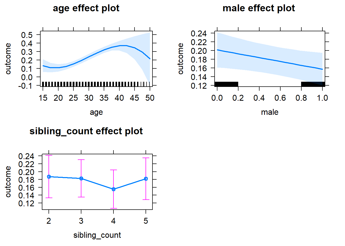
Add Birth Order Linear
Model Summary
tidy(m2_birthorder_linear, conf.int = T, conf.level = 0.995)| effect | group | term | estimate | std.error | statistic | df | p.value | conf.low | conf.high |
|---|---|---|---|---|---|---|---|---|---|
| fixed | NA | (Intercept) | 1.05 | 0.3273 | 3.207 | 2530 | 0.001357 | 0.131 | 1.968 |
| fixed | NA | birth_order | -0.0005907 | 0.007493 | -0.07884 | 2399 | 0.9372 | -0.02162 | 0.02044 |
| fixed | NA | poly(age, 3, raw = TRUE)1 | -0.113 | 0.03627 | -3.117 | 2530 | 0.001848 | -0.2148 | -0.01124 |
| fixed | NA | poly(age, 3, raw = TRUE)2 | 0.004359 | 0.001286 | 3.39 | 2530 | 0.0007105 | 0.0007493 | 0.00797 |
| fixed | NA | poly(age, 3, raw = TRUE)3 | -0.00004837 | 0.00001461 | -3.31 | 2530 | 0.0009453 | -0.00008938 | -0.000007352 |
| fixed | NA | male | -0.04433 | 0.01541 | -2.877 | 2481 | 0.004051 | -0.08759 | -0.001076 |
| fixed | NA | sibling_count3 | -0.004297 | 0.0234 | -0.1836 | 2064 | 0.8543 | -0.06998 | 0.06139 |
| fixed | NA | sibling_count4 | -0.03166 | 0.02453 | -1.291 | 2036 | 0.1969 | -0.1005 | 0.03719 |
| fixed | NA | sibling_count5 | -0.004735 | 0.02761 | -0.1715 | 2046 | 0.8639 | -0.08223 | 0.07276 |
| ran_pars | mother_pidlink | sd__(Intercept) | 0.1675 | NA | NA | NA | NA | NA | NA |
| ran_pars | Residual | sd__Observation | 0.3479 | NA | NA | NA | NA | NA | NA |
Coefficient Plot
plot_birthorder2(m2_birthorder_linear, separate = FALSE)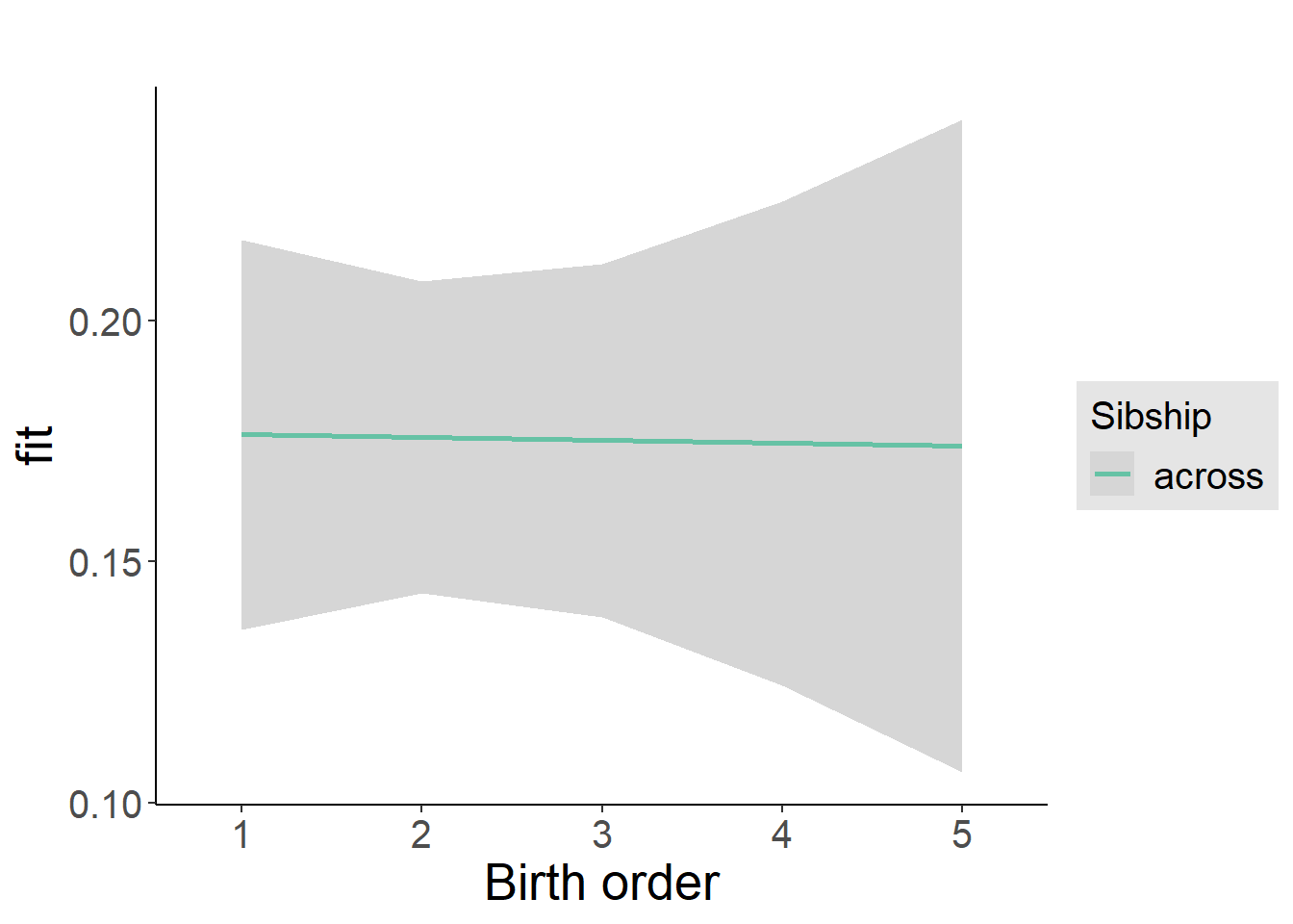
Add Birth Order Factor
Model Summary
m3_birthorder_nonlinear = update(m1_covariates_only, formula = . ~ . + birth_order_nonlinear)
tidy(m3_birthorder_nonlinear, conf.int = T, conf.level = 0.995)| effect | group | term | estimate | std.error | statistic | df | p.value | conf.low | conf.high |
|---|---|---|---|---|---|---|---|---|---|
| fixed | NA | (Intercept) | 1.054 | 0.3282 | 3.212 | 2527 | 0.001335 | 0.1329 | 1.975 |
| fixed | NA | poly(age, 3, raw = TRUE)1 | -0.1141 | 0.03636 | -3.139 | 2527 | 0.001714 | -0.2162 | -0.01208 |
| fixed | NA | poly(age, 3, raw = TRUE)2 | 0.004394 | 0.001289 | 3.408 | 2527 | 0.0006646 | 0.0007749 | 0.008013 |
| fixed | NA | poly(age, 3, raw = TRUE)3 | -0.00004871 | 0.00001465 | -3.326 | 2527 | 0.0008931 | -0.00008982 | -0.000007603 |
| fixed | NA | male | -0.04453 | 0.01542 | -2.888 | 2478 | 0.003913 | -0.08782 | -0.001246 |
| fixed | NA | sibling_count3 | -0.001584 | 0.02372 | -0.0668 | 2109 | 0.9467 | -0.06817 | 0.065 |
| fixed | NA | sibling_count4 | -0.02968 | 0.02481 | -1.196 | 2077 | 0.2317 | -0.09933 | 0.03997 |
| fixed | NA | sibling_count5 | -0.002534 | 0.02777 | -0.09124 | 2064 | 0.9273 | -0.08049 | 0.07542 |
| fixed | NA | birth_order_nonlinear2 | 0.01805 | 0.01822 | 0.9904 | 2121 | 0.3221 | -0.03311 | 0.06921 |
| fixed | NA | birth_order_nonlinear3 | -0.01218 | 0.02252 | -0.5409 | 2207 | 0.5886 | -0.07539 | 0.05103 |
| fixed | NA | birth_order_nonlinear4 | 0.004847 | 0.02955 | 0.164 | 2254 | 0.8697 | -0.0781 | 0.08779 |
| fixed | NA | birth_order_nonlinear5 | 0.002927 | 0.04218 | 0.06938 | 2178 | 0.9447 | -0.1155 | 0.1213 |
| ran_pars | mother_pidlink | sd__(Intercept) | 0.1676 | NA | NA | NA | NA | NA | NA |
| ran_pars | Residual | sd__Observation | 0.348 | NA | NA | NA | NA | NA | NA |
Coefficient Plot
plot_birthorder(m3_birthorder_nonlinear, separate = FALSE)
Add Interaction
Model Summary
m4_interaction = update(m3_birthorder_nonlinear, formula = . ~ . - birth_order_nonlinear - sibling_count + count_birth_order)
tidy(m4_interaction, conf.int = T, conf.level = 0.995)| effect | group | term | estimate | std.error | statistic | df | p.value | conf.low | conf.high |
|---|---|---|---|---|---|---|---|---|---|
| fixed | NA | (Intercept) | 1.035 | 0.3284 | 3.15 | 2521 | 0.001649 | 0.1128 | 1.957 |
| fixed | NA | poly(age, 3, raw = TRUE)1 | -0.1142 | 0.03639 | -3.138 | 2521 | 0.001723 | -0.2163 | -0.01203 |
| fixed | NA | poly(age, 3, raw = TRUE)2 | 0.004394 | 0.00129 | 3.405 | 2521 | 0.0006717 | 0.0007717 | 0.008016 |
| fixed | NA | poly(age, 3, raw = TRUE)3 | -0.0000487 | 0.00001466 | -3.323 | 2521 | 0.0009044 | -0.00008985 | -0.000007557 |
| fixed | NA | male | -0.04493 | 0.01545 | -2.908 | 2473 | 0.003673 | -0.0883 | -0.001556 |
| fixed | NA | count_birth_order2/2 | 0.08055 | 0.0351 | 2.295 | 2248 | 0.02183 | -0.01798 | 0.1791 |
| fixed | NA | count_birth_order1/3 | 0.02443 | 0.03018 | 0.8094 | 2515 | 0.4184 | -0.06028 | 0.1091 |
| fixed | NA | count_birth_order2/3 | 0.04417 | 0.03276 | 1.348 | 2521 | 0.1777 | -0.0478 | 0.1361 |
| fixed | NA | count_birth_order3/3 | -0.01421 | 0.03599 | -0.3948 | 2516 | 0.693 | -0.1152 | 0.08682 |
| fixed | NA | count_birth_order1/4 | 0.01002 | 0.0329 | 0.3045 | 2519 | 0.7608 | -0.08234 | 0.1024 |
| fixed | NA | count_birth_order2/4 | -0.0249 | 0.03426 | -0.7267 | 2520 | 0.4675 | -0.1211 | 0.07127 |
| fixed | NA | count_birth_order3/4 | -0.008878 | 0.03737 | -0.2375 | 2505 | 0.8123 | -0.1138 | 0.09603 |
| fixed | NA | count_birth_order4/4 | -0.002061 | 0.03984 | -0.05174 | 2499 | 0.9587 | -0.1139 | 0.1098 |
| fixed | NA | count_birth_order1/5 | 0.02277 | 0.03946 | 0.5769 | 2520 | 0.5641 | -0.08801 | 0.1335 |
| fixed | NA | count_birth_order2/5 | 0.02039 | 0.04089 | 0.4985 | 2508 | 0.6182 | -0.0944 | 0.1352 |
| fixed | NA | count_birth_order3/5 | 0.01907 | 0.04154 | 0.4591 | 2494 | 0.6462 | -0.09754 | 0.1357 |
| fixed | NA | count_birth_order4/5 | 0.01981 | 0.04213 | 0.4702 | 2480 | 0.6383 | -0.09846 | 0.1381 |
| fixed | NA | count_birth_order5/5 | 0.02095 | 0.04244 | 0.4937 | 2480 | 0.6215 | -0.09817 | 0.1401 |
| ran_pars | mother_pidlink | sd__(Intercept) | 0.1668 | NA | NA | NA | NA | NA | NA |
| ran_pars | Residual | sd__Observation | 0.3483 | NA | NA | NA | NA | NA | NA |
Coefficient Plot
plot_birthorder(m4_interaction)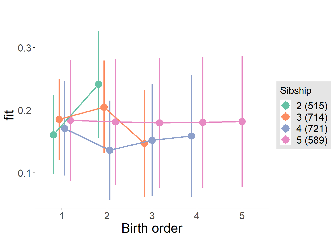
Model Comparison
###### Model 1 - Model 2
anova(m1_covariates_only, m2_birthorder_linear, m3_birthorder_nonlinear, m4_interaction)## refitting model(s) with ML (instead of REML)| Df | AIC | BIC | logLik | deviance | Chisq | Chi Df | Pr(>Chisq) |
|---|---|---|---|---|---|---|---|
| 10 | 2357 | 2415 | -1168 | 2337 | NA | NA | NA |
| 11 | 2359 | 2423 | -1168 | 2337 | 0.006049 | 1 | 0.938 |
| 14 | 2363 | 2445 | -1167 | 2335 | 1.949 | 3 | 0.5831 |
| 20 | 2368 | 2485 | -1164 | 2328 | 6.778 | 6 | 0.3418 |
Parental full sibling order
outcome_parental_m1 <- update(m2_birthorder_linear, data = birthorder %>%
mutate(sibling_count = sibling_count_genes_factor,
birth_order_nonlinear = birthorder_genes_factor,
birth_order = birthorder_genes,
count_birth_order = count_birthorder_genes
) %>%
filter(sibling_count != "1"))
compare_models_markdown(outcome_parental_m1)Basic Model
Model Summary
m1_covariates_only <- update(m2_birthorder_linear, formula = . ~ . - birth_order)
tidy(m1_covariates_only, conf.int = T, conf.level = 0.995)| effect | group | term | estimate | std.error | statistic | df | p.value | conf.low | conf.high |
|---|---|---|---|---|---|---|---|---|---|
| fixed | NA | (Intercept) | 1.218 | 0.3247 | 3.753 | 2759 | 0.0001783 | 0.3071 | 2.13 |
| fixed | NA | poly(age, 3, raw = TRUE)1 | -0.1353 | 0.03606 | -3.752 | 2759 | 0.0001789 | -0.2365 | -0.03408 |
| fixed | NA | poly(age, 3, raw = TRUE)2 | 0.005209 | 0.001282 | 4.064 | 2760 | 0.00004949 | 0.001612 | 0.008807 |
| fixed | NA | poly(age, 3, raw = TRUE)3 | -0.00005869 | 0.0000146 | -4.021 | 2759 | 0.00005948 | -0.00009966 | -0.00001772 |
| fixed | NA | male | -0.03916 | 0.01501 | -2.609 | 2716 | 0.009137 | -0.0813 | 0.002977 |
| fixed | NA | sibling_count3 | 0.02419 | 0.02095 | 1.155 | 2215 | 0.2484 | -0.03461 | 0.08299 |
| fixed | NA | sibling_count4 | -0.02397 | 0.02207 | -1.086 | 2073 | 0.2775 | -0.08592 | 0.03797 |
| fixed | NA | sibling_count5 | 0.03404 | 0.02532 | 1.344 | 1808 | 0.179 | -0.03704 | 0.1051 |
| ran_pars | mother_pidlink | sd__(Intercept) | 0.1622 | NA | NA | NA | NA | NA | NA |
| ran_pars | Residual | sd__Observation | 0.3573 | NA | NA | NA | NA | NA | NA |
Coefficient Plot
plot(allEffects(m1_covariates_only, confidence.level = 0.995))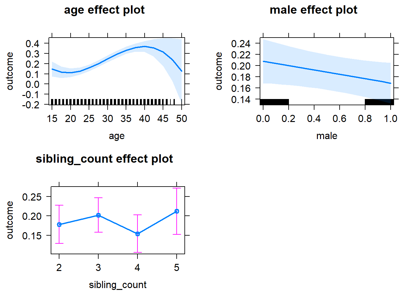
Add Birth Order Linear
Model Summary
tidy(m2_birthorder_linear, conf.int = T, conf.level = 0.995)| effect | group | term | estimate | std.error | statistic | df | p.value | conf.low | conf.high |
|---|---|---|---|---|---|---|---|---|---|
| fixed | NA | (Intercept) | 1.22 | 0.3247 | 3.756 | 2758 | 0.0001759 | 0.3083 | 2.131 |
| fixed | NA | birth_order | -0.003094 | 0.007611 | -0.4066 | 2561 | 0.6844 | -0.02446 | 0.01827 |
| fixed | NA | poly(age, 3, raw = TRUE)1 | -0.1351 | 0.03607 | -3.745 | 2758 | 0.0001842 | -0.2363 | -0.03383 |
| fixed | NA | poly(age, 3, raw = TRUE)2 | 0.005206 | 0.001282 | 4.061 | 2758 | 0.00005019 | 0.001608 | 0.008804 |
| fixed | NA | poly(age, 3, raw = TRUE)3 | -0.00005873 | 0.0000146 | -4.023 | 2759 | 0.00005891 | -0.00009971 | -0.00001776 |
| fixed | NA | male | -0.03919 | 0.01501 | -2.61 | 2714 | 0.009092 | -0.08134 | 0.002952 |
| fixed | NA | sibling_count3 | 0.02571 | 0.02128 | 1.208 | 2242 | 0.2273 | -0.03404 | 0.08545 |
| fixed | NA | sibling_count4 | -0.02081 | 0.0234 | -0.8891 | 2193 | 0.374 | -0.08651 | 0.04489 |
| fixed | NA | sibling_count5 | 0.03922 | 0.02837 | 1.382 | 2085 | 0.167 | -0.04043 | 0.1189 |
| ran_pars | mother_pidlink | sd__(Intercept) | 0.1625 | NA | NA | NA | NA | NA | NA |
| ran_pars | Residual | sd__Observation | 0.3573 | NA | NA | NA | NA | NA | NA |
Coefficient Plot
plot_birthorder2(m2_birthorder_linear, separate = FALSE)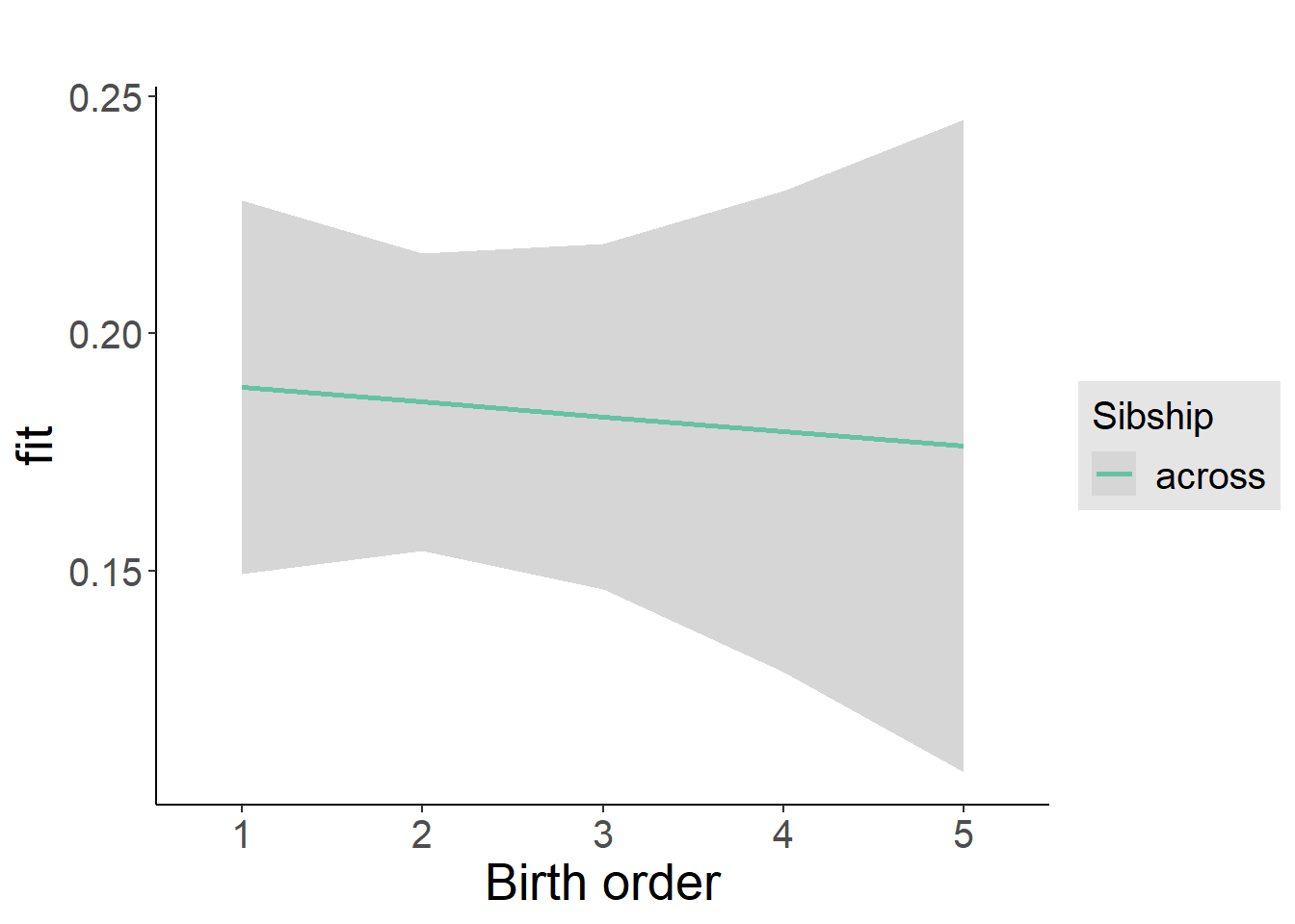
Add Birth Order Factor
Model Summary
m3_birthorder_nonlinear = update(m1_covariates_only, formula = . ~ . + birth_order_nonlinear)
tidy(m3_birthorder_nonlinear, conf.int = T, conf.level = 0.995)| effect | group | term | estimate | std.error | statistic | df | p.value | conf.low | conf.high |
|---|---|---|---|---|---|---|---|---|---|
| fixed | NA | (Intercept) | 1.224 | 0.3254 | 3.762 | 2755 | 0.0001718 | 0.3109 | 2.138 |
| fixed | NA | poly(age, 3, raw = TRUE)1 | -0.1362 | 0.03613 | -3.768 | 2755 | 0.0001678 | -0.2376 | -0.03473 |
| fixed | NA | poly(age, 3, raw = TRUE)2 | 0.005242 | 0.001284 | 4.082 | 2755 | 0.00004584 | 0.001638 | 0.008847 |
| fixed | NA | poly(age, 3, raw = TRUE)3 | -0.00005912 | 0.00001462 | -4.043 | 2756 | 0.00005421 | -0.0001002 | -0.00001807 |
| fixed | NA | male | -0.03964 | 0.01503 | -2.638 | 2712 | 0.008387 | -0.08182 | 0.00254 |
| fixed | NA | sibling_count3 | 0.02762 | 0.02161 | 1.278 | 2300 | 0.2013 | -0.03304 | 0.08827 |
| fixed | NA | sibling_count4 | -0.02282 | 0.0237 | -0.9627 | 2246 | 0.3358 | -0.08935 | 0.04371 |
| fixed | NA | sibling_count5 | 0.04276 | 0.02883 | 1.483 | 2139 | 0.1382 | -0.03816 | 0.1237 |
| fixed | NA | birth_order_nonlinear2 | 0.005778 | 0.01769 | 0.3267 | 2306 | 0.744 | -0.04388 | 0.05543 |
| fixed | NA | birth_order_nonlinear3 | -0.01319 | 0.0218 | -0.6048 | 2374 | 0.5453 | -0.07438 | 0.04801 |
| fixed | NA | birth_order_nonlinear4 | 0.0128 | 0.02985 | 0.4288 | 2430 | 0.6681 | -0.071 | 0.0966 |
| fixed | NA | birth_order_nonlinear5 | -0.04222 | 0.04702 | -0.8979 | 2370 | 0.3693 | -0.1742 | 0.08977 |
| ran_pars | mother_pidlink | sd__(Intercept) | 0.1626 | NA | NA | NA | NA | NA | NA |
| ran_pars | Residual | sd__Observation | 0.3573 | NA | NA | NA | NA | NA | NA |
Coefficient Plot
plot_birthorder(m3_birthorder_nonlinear, separate = FALSE)
Add Interaction
Model Summary
m4_interaction = update(m3_birthorder_nonlinear, formula = . ~ . - birth_order_nonlinear - sibling_count + count_birth_order)
tidy(m4_interaction, conf.int = T, conf.level = 0.995)| effect | group | term | estimate | std.error | statistic | df | p.value | conf.low | conf.high |
|---|---|---|---|---|---|---|---|---|---|
| fixed | NA | (Intercept) | 1.215 | 0.3256 | 3.732 | 2749 | 0.0001938 | 0.3012 | 2.129 |
| fixed | NA | poly(age, 3, raw = TRUE)1 | -0.1366 | 0.03616 | -3.777 | 2749 | 0.0001618 | -0.2381 | -0.03509 |
| fixed | NA | poly(age, 3, raw = TRUE)2 | 0.005262 | 0.001285 | 4.094 | 2749 | 0.00004364 | 0.001654 | 0.008869 |
| fixed | NA | poly(age, 3, raw = TRUE)3 | -0.00005939 | 0.00001464 | -4.057 | 2750 | 0.000051 | -0.0001005 | -0.0000183 |
| fixed | NA | male | -0.0399 | 0.01505 | -2.652 | 2706 | 0.008054 | -0.08213 | 0.002336 |
| fixed | NA | count_birth_order2/2 | 0.04292 | 0.03156 | 1.36 | 2372 | 0.174 | -0.04567 | 0.1315 |
| fixed | NA | count_birth_order1/3 | 0.0477 | 0.0273 | 1.747 | 2744 | 0.08069 | -0.02893 | 0.1243 |
| fixed | NA | count_birth_order2/3 | 0.04547 | 0.03031 | 1.5 | 2749 | 0.1337 | -0.03962 | 0.1306 |
| fixed | NA | count_birth_order3/3 | 0.01206 | 0.03243 | 0.3719 | 2743 | 0.71 | -0.07898 | 0.1031 |
| fixed | NA | count_birth_order1/4 | -0.005346 | 0.03208 | -0.1667 | 2750 | 0.8677 | -0.09539 | 0.0847 |
| fixed | NA | count_birth_order2/4 | -0.03738 | 0.03344 | -1.118 | 2745 | 0.2638 | -0.1312 | 0.05649 |
| fixed | NA | count_birth_order3/4 | -0.009675 | 0.03502 | -0.2763 | 2734 | 0.7824 | -0.108 | 0.08863 |
| fixed | NA | count_birth_order4/4 | 0.02324 | 0.03772 | 0.6161 | 2730 | 0.5379 | -0.08265 | 0.1291 |
| fixed | NA | count_birth_order1/5 | 0.0641 | 0.04203 | 1.525 | 2748 | 0.1273 | -0.05388 | 0.1821 |
| fixed | NA | count_birth_order2/5 | 0.07532 | 0.04698 | 1.603 | 2707 | 0.109 | -0.05657 | 0.2072 |
| fixed | NA | count_birth_order3/5 | 0.04924 | 0.04493 | 1.096 | 2710 | 0.2732 | -0.07688 | 0.1754 |
| fixed | NA | count_birth_order4/5 | 0.03861 | 0.04329 | 0.8917 | 2714 | 0.3726 | -0.08292 | 0.1601 |
| fixed | NA | count_birth_order5/5 | 0.01255 | 0.04555 | 0.2754 | 2707 | 0.783 | -0.1153 | 0.1404 |
| ran_pars | mother_pidlink | sd__(Intercept) | 0.1622 | NA | NA | NA | NA | NA | NA |
| ran_pars | Residual | sd__Observation | 0.3576 | NA | NA | NA | NA | NA | NA |
Coefficient Plot
plot_birthorder(m4_interaction)
Model Comparison
###### Model 1 - Model 2
anova(m1_covariates_only, m2_birthorder_linear, m3_birthorder_nonlinear, m4_interaction)## refitting model(s) with ML (instead of REML)| Df | AIC | BIC | logLik | deviance | Chisq | Chi Df | Pr(>Chisq) |
|---|---|---|---|---|---|---|---|
| 10 | 2663 | 2722 | -1322 | 2643 | NA | NA | NA |
| 11 | 2665 | 2730 | -1321 | 2643 | 0.1642 | 1 | 0.6853 |
| 14 | 2669 | 2752 | -1321 | 2641 | 1.786 | 3 | 0.618 |
| 20 | 2676 | 2795 | -1318 | 2636 | 4.918 | 6 | 0.5544 |
Compare birth order specifications
library(coefplot)
multiplot(outcome_naive_m1, outcome_preg_m1, outcome_uterus_m1, outcome_parental_m1, dodgeHeight = 0.6,
intercept = FALSE)
Work Category
Category_Casual worker in agriculture
birthorder <- birthorder %>% mutate(outcome = `Category_Casual worker in agriculture`)
model = lmer(outcome ~ birth_order + poly(age, 3, raw = TRUE) + male + sibling_count + (1 | mother_pidlink),
data = birthorder)
compare_birthorder_specs(model)Naive birth order
outcome_naive_m1 <- update(m2_birthorder_linear, data = birthorder %>%
mutate(sibling_count = sibling_count_naive_factor,
birth_order_nonlinear = birthorder_naive_factor,
birth_order = birthorder_naive,
count_birth_order = count_birthorder_naive) %>%
filter(sibling_count != "1"))
compare_models_markdown(outcome_naive_m1)Basic Model
Model Summary
m1_covariates_only <- update(m2_birthorder_linear, formula = . ~ . - birth_order)
tidy(m1_covariates_only, conf.int = T, conf.level = 0.995)| effect | group | term | estimate | std.error | statistic | df | p.value | conf.low | conf.high |
|---|---|---|---|---|---|---|---|---|---|
| fixed | NA | (Intercept) | 0.1194 | 0.04345 | 2.748 | 4366 | 0.006022 | -0.002568 | 0.2414 |
| fixed | NA | poly(age, 3, raw = TRUE)1 | -0.009701 | 0.003871 | -2.506 | 4224 | 0.01224 | -0.02057 | 0.001165 |
| fixed | NA | poly(age, 3, raw = TRUE)2 | 0.0002729 | 0.0001074 | 2.542 | 4068 | 0.01105 | -0.00002842 | 0.0005743 |
| fixed | NA | poly(age, 3, raw = TRUE)3 | -0.000002212 | 0.0000009378 | -2.359 | 3934 | 0.01838 | -0.000004844 | 0.0000004203 |
| fixed | NA | male | 0.003536 | 0.004449 | 0.7948 | 4797 | 0.4268 | -0.008952 | 0.01602 |
| fixed | NA | sibling_count3 | -0.002646 | 0.006308 | -0.4195 | 3380 | 0.6749 | -0.02035 | 0.01506 |
| fixed | NA | sibling_count4 | 0.006909 | 0.006365 | 1.085 | 3103 | 0.2778 | -0.01096 | 0.02478 |
| fixed | NA | sibling_count5 | -0.001435 | 0.006628 | -0.2165 | 2826 | 0.8286 | -0.02004 | 0.01717 |
| ran_pars | mother_pidlink | sd__(Intercept) | 0.03829 | NA | NA | NA | NA | NA | NA |
| ran_pars | Residual | sd__Observation | 0.1482 | NA | NA | NA | NA | NA | NA |
Coefficient Plot
plot(allEffects(m1_covariates_only, confidence.level = 0.995))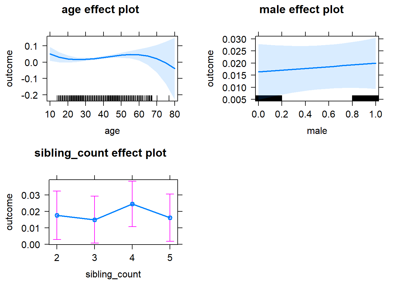
Add Birth Order Linear
Model Summary
tidy(m2_birthorder_linear, conf.int = T, conf.level = 0.995)| effect | group | term | estimate | std.error | statistic | df | p.value | conf.low | conf.high |
|---|---|---|---|---|---|---|---|---|---|
| fixed | NA | (Intercept) | 0.1193 | 0.04346 | 2.745 | 4366 | 0.006072 | -0.002687 | 0.2413 |
| fixed | NA | birth_order | -0.0005024 | 0.002196 | -0.2288 | 4298 | 0.819 | -0.006666 | 0.005661 |
| fixed | NA | poly(age, 3, raw = TRUE)1 | -0.009627 | 0.003885 | -2.478 | 4224 | 0.01324 | -0.02053 | 0.001277 |
| fixed | NA | poly(age, 3, raw = TRUE)2 | 0.0002711 | 0.0001077 | 2.518 | 4059 | 0.01184 | -0.00003112 | 0.0005733 |
| fixed | NA | poly(age, 3, raw = TRUE)3 | -0.0000022 | 0.0000009394 | -2.342 | 3926 | 0.01924 | -0.000004837 | 0.000000437 |
| fixed | NA | male | 0.003531 | 0.004449 | 0.7936 | 4796 | 0.4275 | -0.008958 | 0.01602 |
| fixed | NA | sibling_count3 | -0.002452 | 0.006365 | -0.3853 | 3476 | 0.7001 | -0.02032 | 0.01542 |
| fixed | NA | sibling_count4 | 0.00732 | 0.006614 | 1.107 | 3491 | 0.2685 | -0.01125 | 0.02589 |
| fixed | NA | sibling_count5 | -0.000781 | 0.007218 | -0.1082 | 3605 | 0.9138 | -0.02104 | 0.01948 |
| ran_pars | mother_pidlink | sd__(Intercept) | 0.03825 | NA | NA | NA | NA | NA | NA |
| ran_pars | Residual | sd__Observation | 0.1482 | NA | NA | NA | NA | NA | NA |
Coefficient Plot
plot_birthorder2(m2_birthorder_linear, separate = FALSE)
Add Birth Order Factor
Model Summary
m3_birthorder_nonlinear = update(m1_covariates_only, formula = . ~ . + birth_order_nonlinear)
tidy(m3_birthorder_nonlinear, conf.int = T, conf.level = 0.995)| effect | group | term | estimate | std.error | statistic | df | p.value | conf.low | conf.high |
|---|---|---|---|---|---|---|---|---|---|
| fixed | NA | (Intercept) | 0.1221 | 0.04357 | 2.801 | 4370 | 0.005113 | -0.0002515 | 0.2444 |
| fixed | NA | poly(age, 3, raw = TRUE)1 | -0.009769 | 0.003885 | -2.514 | 4218 | 0.01196 | -0.02067 | 0.001137 |
| fixed | NA | poly(age, 3, raw = TRUE)2 | 0.0002768 | 0.0001077 | 2.57 | 4048 | 0.0102 | -0.00002551 | 0.0005791 |
| fixed | NA | poly(age, 3, raw = TRUE)3 | -0.000002264 | 0.00000094 | -2.408 | 3908 | 0.01606 | -0.000004903 | 0.0000003746 |
| fixed | NA | male | 0.003518 | 0.00445 | 0.7906 | 4793 | 0.4292 | -0.008974 | 0.01601 |
| fixed | NA | sibling_count3 | -0.001917 | 0.006481 | -0.2958 | 3643 | 0.7674 | -0.02011 | 0.01627 |
| fixed | NA | sibling_count4 | 0.005823 | 0.006736 | 0.8644 | 3666 | 0.3874 | -0.01309 | 0.02473 |
| fixed | NA | sibling_count5 | -0.001364 | 0.007292 | -0.1871 | 3710 | 0.8516 | -0.02183 | 0.0191 |
| fixed | NA | birth_order_nonlinear2 | -0.006773 | 0.005299 | -1.278 | 4172 | 0.2012 | -0.02165 | 0.008101 |
| fixed | NA | birth_order_nonlinear3 | -0.004748 | 0.006743 | -0.7041 | 4149 | 0.4814 | -0.02368 | 0.01418 |
| fixed | NA | birth_order_nonlinear4 | 0.007102 | 0.008757 | 0.8111 | 4144 | 0.4174 | -0.01748 | 0.03168 |
| fixed | NA | birth_order_nonlinear5 | -0.00871 | 0.01265 | -0.6886 | 4183 | 0.4911 | -0.04421 | 0.02679 |
| ran_pars | mother_pidlink | sd__(Intercept) | 0.03817 | NA | NA | NA | NA | NA | NA |
| ran_pars | Residual | sd__Observation | 0.1482 | NA | NA | NA | NA | NA | NA |
Coefficient Plot
plot_birthorder(m3_birthorder_nonlinear, separate = FALSE)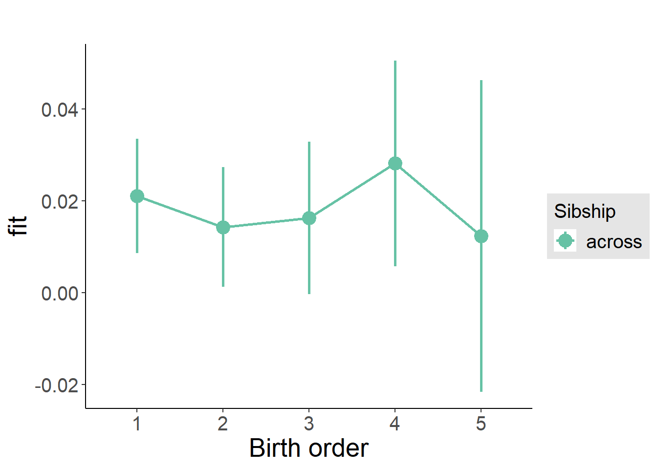
Add Interaction
Model Summary
m4_interaction = update(m3_birthorder_nonlinear, formula = . ~ . - birth_order_nonlinear - sibling_count + count_birth_order)
tidy(m4_interaction, conf.int = T, conf.level = 0.995)| effect | group | term | estimate | std.error | statistic | df | p.value | conf.low | conf.high |
|---|---|---|---|---|---|---|---|---|---|
| fixed | NA | (Intercept) | 0.1229 | 0.04363 | 2.817 | 4376 | 0.004877 | 0.0004131 | 0.2454 |
| fixed | NA | poly(age, 3, raw = TRUE)1 | -0.009585 | 0.003887 | -2.466 | 4215 | 0.01371 | -0.0205 | 0.001326 |
| fixed | NA | poly(age, 3, raw = TRUE)2 | 0.0002733 | 0.0001077 | 2.537 | 4045 | 0.01121 | -0.00002905 | 0.0005756 |
| fixed | NA | poly(age, 3, raw = TRUE)3 | -0.00000225 | 0.00000094 | -2.393 | 3904 | 0.01674 | -0.000004888 | 0.0000003887 |
| fixed | NA | male | 0.003589 | 0.004451 | 0.8063 | 4785 | 0.4201 | -0.008905 | 0.01608 |
| fixed | NA | count_birth_order2/2 | -0.01581 | 0.009004 | -1.756 | 4070 | 0.07909 | -0.04109 | 0.009459 |
| fixed | NA | count_birth_order1/3 | -0.006721 | 0.008603 | -0.7812 | 4801 | 0.4347 | -0.03087 | 0.01743 |
| fixed | NA | count_birth_order2/3 | -0.006495 | 0.009548 | -0.6803 | 4805 | 0.4963 | -0.0333 | 0.02031 |
| fixed | NA | count_birth_order3/3 | -0.01486 | 0.01051 | -1.414 | 4806 | 0.1575 | -0.04436 | 0.01464 |
| fixed | NA | count_birth_order1/4 | -0.007151 | 0.009439 | -0.7576 | 4805 | 0.4487 | -0.03365 | 0.01934 |
| fixed | NA | count_birth_order2/4 | -0.002565 | 0.01013 | -0.2533 | 4806 | 0.8001 | -0.03099 | 0.02586 |
| fixed | NA | count_birth_order3/4 | 0.01192 | 0.01081 | 1.103 | 4806 | 0.2701 | -0.01842 | 0.04226 |
| fixed | NA | count_birth_order4/4 | 0.006717 | 0.0115 | 0.5842 | 4806 | 0.5591 | -0.02556 | 0.03899 |
| fixed | NA | count_birth_order1/5 | 0.002831 | 0.01073 | 0.264 | 4806 | 0.7918 | -0.02727 | 0.03294 |
| fixed | NA | count_birth_order2/5 | -0.01267 | 0.01139 | -1.112 | 4805 | 0.2661 | -0.04463 | 0.0193 |
| fixed | NA | count_birth_order3/5 | -0.02166 | 0.01199 | -1.807 | 4805 | 0.0709 | -0.05532 | 0.012 |
| fixed | NA | count_birth_order4/5 | 0.005769 | 0.01262 | 0.4571 | 4800 | 0.6476 | -0.02966 | 0.04119 |
| fixed | NA | count_birth_order5/5 | -0.01361 | 0.01262 | -1.079 | 4804 | 0.2809 | -0.04904 | 0.02182 |
| ran_pars | mother_pidlink | sd__(Intercept) | 0.03829 | NA | NA | NA | NA | NA | NA |
| ran_pars | Residual | sd__Observation | 0.1481 | NA | NA | NA | NA | NA | NA |
Coefficient Plot
plot_birthorder(m4_interaction)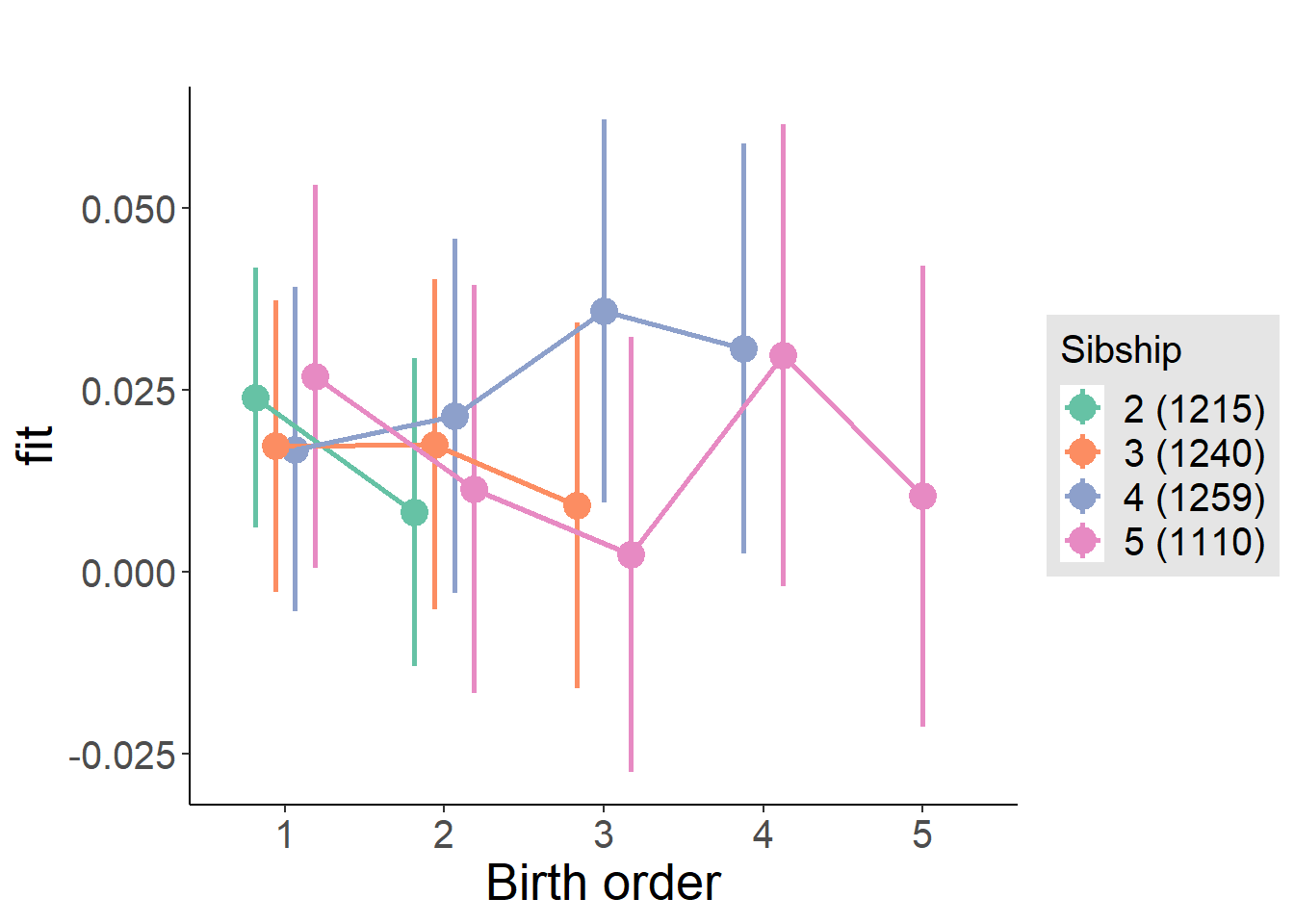
Model Comparison
###### Model 1 - Model 2
anova(m1_covariates_only, m2_birthorder_linear, m3_birthorder_nonlinear, m4_interaction)## refitting model(s) with ML (instead of REML)| Df | AIC | BIC | logLik | deviance | Chisq | Chi Df | Pr(>Chisq) |
|---|---|---|---|---|---|---|---|
| 10 | -4415 | -4350 | 2218 | -4435 | NA | NA | NA |
| 11 | -4413 | -4342 | 2218 | -4435 | 0.05262 | 1 | 0.8186 |
| 14 | -4411 | -4320 | 2219 | -4439 | 3.738 | 3 | 0.2911 |
| 20 | -4407 | -4278 | 2224 | -4447 | 8.343 | 6 | 0.214 |
Maternal birth order
outcome_uterus_m1 <- update(m2_birthorder_linear, data = birthorder %>%
mutate(sibling_count = sibling_count_uterus_alive_factor,
birth_order_nonlinear = birthorder_uterus_alive_factor,
birth_order = birthorder_uterus_alive,
count_birth_order = count_birthorder_uterus_alive) %>%
filter(sibling_count != "1"))## boundary (singular) fit: see ?isSingularcompare_models_markdown(outcome_uterus_m1)Basic Model
Model Summary
m1_covariates_only <- update(m2_birthorder_linear, formula = . ~ . - birth_order)## boundary (singular) fit: see ?isSingulartidy(m1_covariates_only, conf.int = T, conf.level = 0.995)| effect | group | term | estimate | std.error | statistic | df | p.value | conf.low | conf.high |
|---|---|---|---|---|---|---|---|---|---|
| fixed | NA | (Intercept) | -0.03756 | 0.08345 | -0.4501 | 2760 | 0.6527 | -0.2718 | 0.1967 |
| fixed | NA | poly(age, 3, raw = TRUE)1 | 0.007165 | 0.009243 | 0.7752 | 2760 | 0.4383 | -0.01878 | 0.03311 |
| fixed | NA | poly(age, 3, raw = TRUE)2 | -0.0003047 | 0.0003277 | -0.9298 | 2760 | 0.3525 | -0.001225 | 0.0006152 |
| fixed | NA | poly(age, 3, raw = TRUE)3 | 0.000003864 | 0.000003721 | 1.038 | 2760 | 0.2992 | -0.000006582 | 0.00001431 |
| fixed | NA | male | 0.004517 | 0.00393 | 1.149 | 2760 | 0.2505 | -0.006516 | 0.01555 |
| fixed | NA | sibling_count3 | -0.005617 | 0.005383 | -1.044 | 2760 | 0.2968 | -0.02073 | 0.009493 |
| fixed | NA | sibling_count4 | -0.0001364 | 0.005558 | -0.02454 | 2760 | 0.9804 | -0.01574 | 0.01546 |
| fixed | NA | sibling_count5 | -0.006986 | 0.006138 | -1.138 | 2760 | 0.2552 | -0.02422 | 0.01024 |
| ran_pars | mother_pidlink | sd__(Intercept) | 0 | NA | NA | NA | NA | NA | NA |
| ran_pars | Residual | sd__Observation | 0.1018 | NA | NA | NA | NA | NA | NA |
Coefficient Plot
plot(allEffects(m1_covariates_only, confidence.level = 0.995))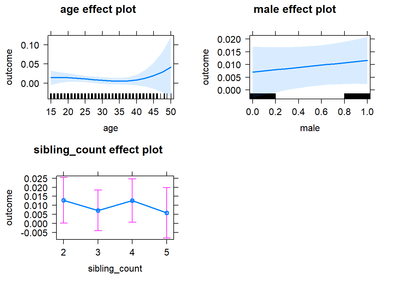
Add Birth Order Linear
Model Summary
tidy(m2_birthorder_linear, conf.int = T, conf.level = 0.995)| effect | group | term | estimate | std.error | statistic | df | p.value | conf.low | conf.high |
|---|---|---|---|---|---|---|---|---|---|
| fixed | NA | (Intercept) | -0.0377 | 0.08347 | -0.4517 | 2759 | 0.6515 | -0.272 | 0.1966 |
| fixed | NA | birth_order | 0.0002319 | 0.001991 | 0.1165 | 2759 | 0.9073 | -0.005357 | 0.005821 |
| fixed | NA | poly(age, 3, raw = TRUE)1 | 0.007154 | 0.009245 | 0.7738 | 2759 | 0.4391 | -0.0188 | 0.03311 |
| fixed | NA | poly(age, 3, raw = TRUE)2 | -0.0003047 | 0.0003278 | -0.9297 | 2759 | 0.3526 | -0.001225 | 0.0006154 |
| fixed | NA | poly(age, 3, raw = TRUE)3 | 0.00000387 | 0.000003722 | 1.04 | 2759 | 0.2986 | -0.000006579 | 0.00001432 |
| fixed | NA | male | 0.004518 | 0.003931 | 1.149 | 2759 | 0.2505 | -0.006517 | 0.01555 |
| fixed | NA | sibling_count3 | -0.005729 | 0.005469 | -1.048 | 2759 | 0.2949 | -0.02108 | 0.009622 |
| fixed | NA | sibling_count4 | -0.0003731 | 0.005919 | -0.06304 | 2759 | 0.9497 | -0.01699 | 0.01624 |
| fixed | NA | sibling_count5 | -0.007385 | 0.00703 | -1.051 | 2759 | 0.2935 | -0.02712 | 0.01235 |
| ran_pars | mother_pidlink | sd__(Intercept) | 0 | NA | NA | NA | NA | NA | NA |
| ran_pars | Residual | sd__Observation | 0.1018 | NA | NA | NA | NA | NA | NA |
Coefficient Plot
plot_birthorder2(m2_birthorder_linear, separate = FALSE)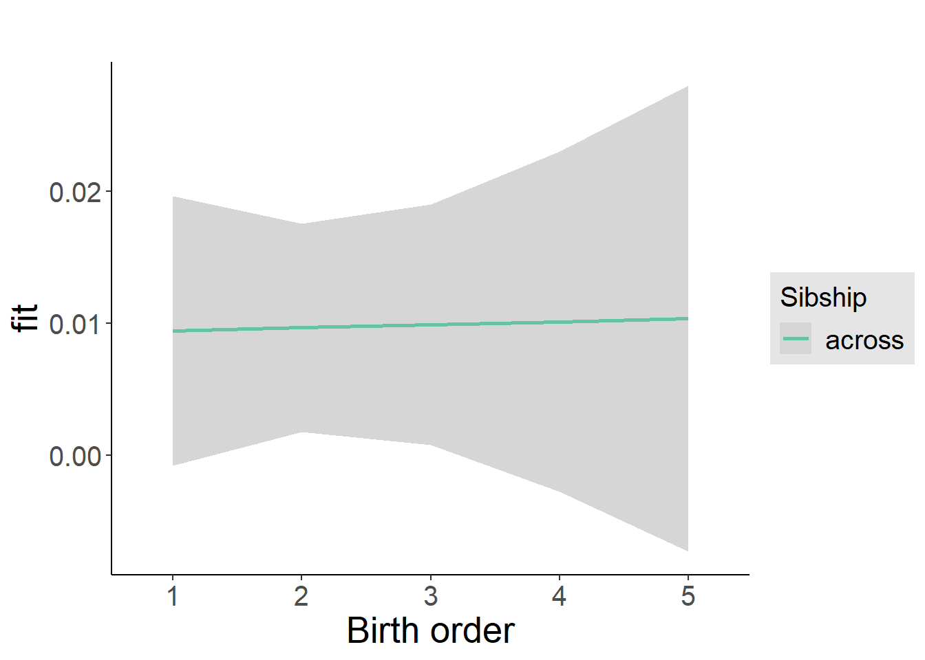
Add Birth Order Factor
Model Summary
m3_birthorder_nonlinear = update(m1_covariates_only, formula = . ~ . + birth_order_nonlinear)## boundary (singular) fit: see ?isSingulartidy(m3_birthorder_nonlinear, conf.int = T, conf.level = 0.995)| effect | group | term | estimate | std.error | statistic | df | p.value | conf.low | conf.high |
|---|---|---|---|---|---|---|---|---|---|
| fixed | NA | (Intercept) | -0.03042 | 0.08362 | -0.3638 | 2756 | 0.716 | -0.2652 | 0.2043 |
| fixed | NA | poly(age, 3, raw = TRUE)1 | 0.006443 | 0.00926 | 0.6957 | 2756 | 0.4867 | -0.01955 | 0.03244 |
| fixed | NA | poly(age, 3, raw = TRUE)2 | -0.0002796 | 0.0003283 | -0.8515 | 2756 | 0.3946 | -0.001201 | 0.000642 |
| fixed | NA | poly(age, 3, raw = TRUE)3 | 0.000003596 | 0.000003728 | 0.9646 | 2756 | 0.3348 | -0.000006869 | 0.00001406 |
| fixed | NA | male | 0.004352 | 0.003933 | 1.107 | 2756 | 0.2685 | -0.006687 | 0.01539 |
| fixed | NA | sibling_count3 | -0.004866 | 0.00556 | -0.8753 | 2756 | 0.3815 | -0.02047 | 0.01074 |
| fixed | NA | sibling_count4 | -0.001313 | 0.006005 | -0.2187 | 2756 | 0.8269 | -0.01817 | 0.01554 |
| fixed | NA | sibling_count5 | -0.007485 | 0.007125 | -1.051 | 2756 | 0.2936 | -0.02749 | 0.01252 |
| fixed | NA | birth_order_nonlinear2 | -0.002069 | 0.004788 | -0.4321 | 2756 | 0.6657 | -0.01551 | 0.01137 |
| fixed | NA | birth_order_nonlinear3 | -0.003443 | 0.005834 | -0.5901 | 2756 | 0.5552 | -0.01982 | 0.01293 |
| fixed | NA | birth_order_nonlinear4 | 0.008968 | 0.007732 | 1.16 | 2756 | 0.2462 | -0.01274 | 0.03067 |
| fixed | NA | birth_order_nonlinear5 | -0.006203 | 0.01189 | -0.5216 | 2756 | 0.602 | -0.03958 | 0.02718 |
| ran_pars | mother_pidlink | sd__(Intercept) | 0 | NA | NA | NA | NA | NA | NA |
| ran_pars | Residual | sd__Observation | 0.1018 | NA | NA | NA | NA | NA | NA |
Coefficient Plot
plot_birthorder(m3_birthorder_nonlinear, separate = FALSE)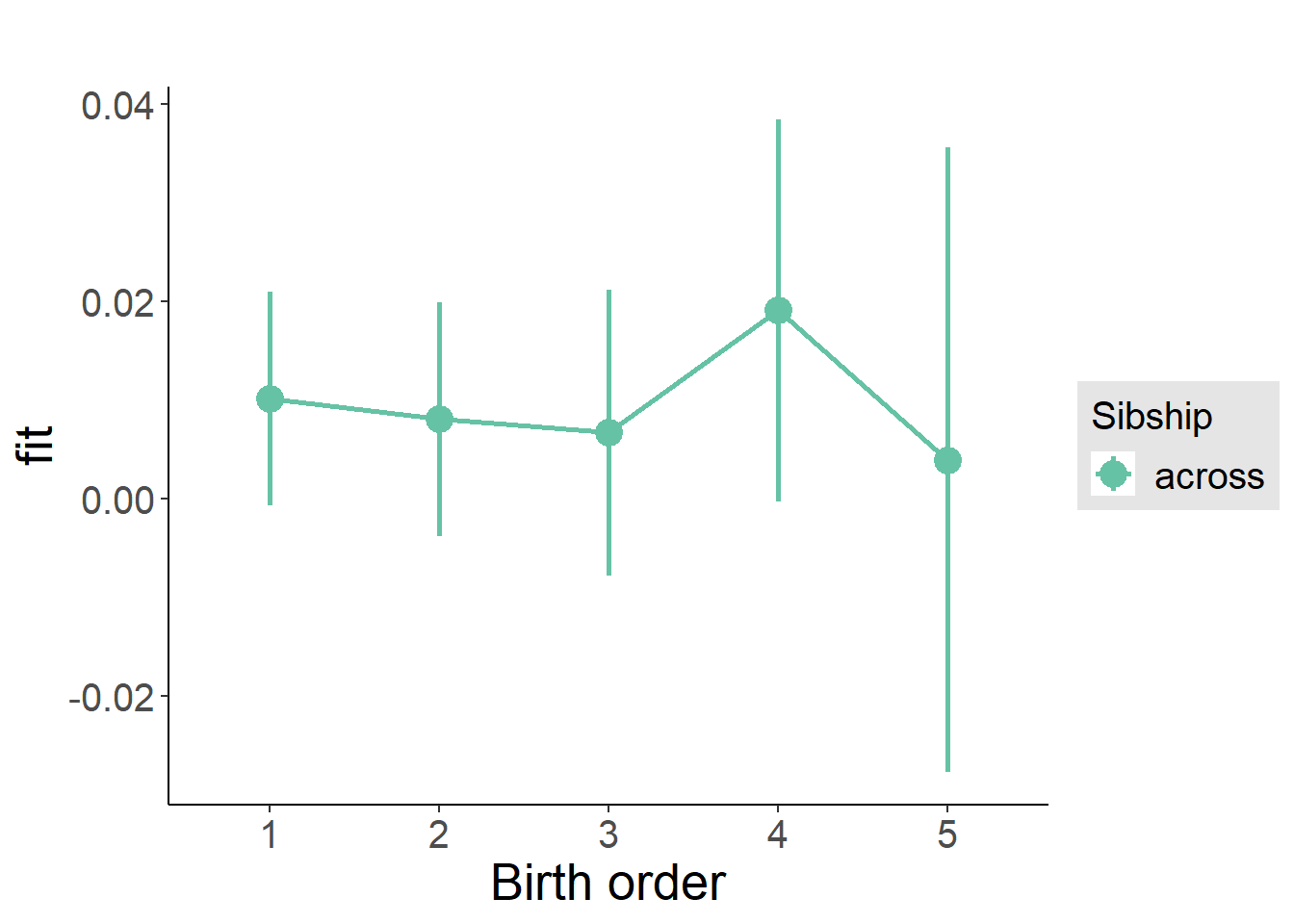
Add Interaction
Model Summary
m4_interaction = update(m3_birthorder_nonlinear, formula = . ~ . - birth_order_nonlinear - sibling_count + count_birth_order)## boundary (singular) fit: see ?isSingulartidy(m4_interaction, conf.int = T, conf.level = 0.995)| effect | group | term | estimate | std.error | statistic | df | p.value | conf.low | conf.high |
|---|---|---|---|---|---|---|---|---|---|
| fixed | NA | (Intercept) | -0.03194 | 0.08369 | -0.3817 | 2750 | 0.7027 | -0.2669 | 0.203 |
| fixed | NA | poly(age, 3, raw = TRUE)1 | 0.006732 | 0.009267 | 0.7265 | 2750 | 0.4676 | -0.01928 | 0.03275 |
| fixed | NA | poly(age, 3, raw = TRUE)2 | -0.0002877 | 0.0003286 | -0.8755 | 2750 | 0.3814 | -0.00121 | 0.0006347 |
| fixed | NA | poly(age, 3, raw = TRUE)3 | 0.00000366 | 0.000003732 | 0.9809 | 2750 | 0.3267 | -0.000006814 | 0.00001413 |
| fixed | NA | male | 0.004362 | 0.003939 | 1.107 | 2750 | 0.2682 | -0.006694 | 0.01542 |
| fixed | NA | count_birth_order2/2 | -0.006758 | 0.008685 | -0.7781 | 2750 | 0.4366 | -0.03114 | 0.01762 |
| fixed | NA | count_birth_order1/3 | -0.01106 | 0.007223 | -1.531 | 2750 | 0.126 | -0.03133 | 0.00922 |
| fixed | NA | count_birth_order2/3 | -0.008417 | 0.008029 | -1.048 | 2750 | 0.2945 | -0.03095 | 0.01412 |
| fixed | NA | count_birth_order3/3 | -0.001227 | 0.008694 | -0.1411 | 2750 | 0.8878 | -0.02563 | 0.02318 |
| fixed | NA | count_birth_order1/4 | 0.001133 | 0.008323 | 0.1362 | 2750 | 0.8917 | -0.02223 | 0.0245 |
| fixed | NA | count_birth_order2/4 | -0.0005705 | 0.008751 | -0.06519 | 2750 | 0.948 | -0.02513 | 0.02399 |
| fixed | NA | count_birth_order3/4 | -0.01496 | 0.009184 | -1.628 | 2750 | 0.1035 | -0.04074 | 0.01082 |
| fixed | NA | count_birth_order4/4 | 0.004138 | 0.00973 | 0.4253 | 2750 | 0.6707 | -0.02318 | 0.03145 |
| fixed | NA | count_birth_order1/5 | -0.00724 | 0.01095 | -0.6611 | 2750 | 0.5086 | -0.03798 | 0.0235 |
| fixed | NA | count_birth_order2/5 | -0.01384 | 0.01191 | -1.162 | 2750 | 0.2454 | -0.04727 | 0.01959 |
| fixed | NA | count_birth_order3/5 | -0.01458 | 0.01115 | -1.308 | 2750 | 0.191 | -0.04587 | 0.01671 |
| fixed | NA | count_birth_order4/5 | 0.002521 | 0.01083 | 0.2327 | 2750 | 0.816 | -0.02789 | 0.03293 |
| fixed | NA | count_birth_order5/5 | -0.01524 | 0.01136 | -1.341 | 2750 | 0.18 | -0.04713 | 0.01666 |
| ran_pars | mother_pidlink | sd__(Intercept) | 0.00000000181 | NA | NA | NA | NA | NA | NA |
| ran_pars | Residual | sd__Observation | 0.1019 | NA | NA | NA | NA | NA | NA |
Coefficient Plot
plot_birthorder(m4_interaction)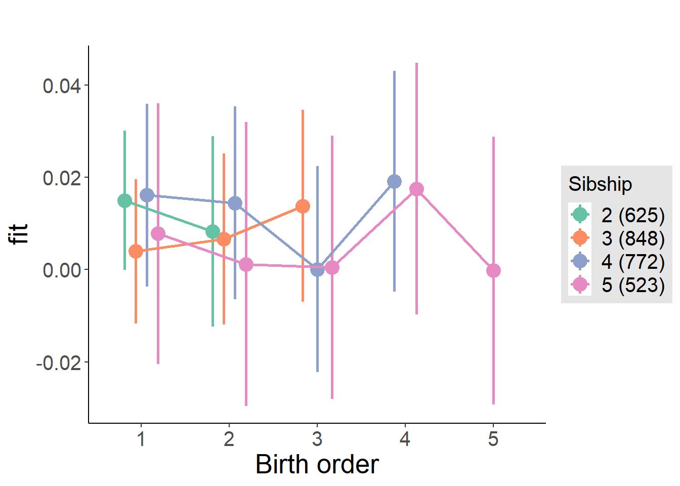
Model Comparison
###### Model 1 - Model 2
anova(m1_covariates_only, m2_birthorder_linear, m3_birthorder_nonlinear, m4_interaction)## refitting model(s) with ML (instead of REML)| Df | AIC | BIC | logLik | deviance | Chisq | Chi Df | Pr(>Chisq) |
|---|---|---|---|---|---|---|---|
| 10 | -4780 | -4721 | 2400 | -4800 | NA | NA | NA |
| 11 | -4778 | -4713 | 2400 | -4800 | 0.01361 | 1 | 0.9071 |
| 14 | -4775 | -4692 | 2402 | -4803 | 3.035 | 3 | 0.3862 |
| 20 | -4768 | -4650 | 2404 | -4808 | 4.873 | 6 | 0.5601 |
Maternal pregnancy order
outcome_preg_m1 <- update(m2_birthorder_linear, data = birthorder %>%
mutate(sibling_count = sibling_count_uterus_preg_factor,
birth_order_nonlinear = birthorder_uterus_preg_factor,
birth_order = birthorder_uterus_preg,
count_birth_order = count_birthorder_uterus_preg
) %>%
filter(sibling_count != "1"))## boundary (singular) fit: see ?isSingularcompare_models_markdown(outcome_preg_m1)Basic Model
Model Summary
m1_covariates_only <- update(m2_birthorder_linear, formula = . ~ . - birth_order)## boundary (singular) fit: see ?isSingulartidy(m1_covariates_only, conf.int = T, conf.level = 0.995)| effect | group | term | estimate | std.error | statistic | df | p.value | conf.low | conf.high |
|---|---|---|---|---|---|---|---|---|---|
| fixed | NA | (Intercept) | -0.03705 | 0.0903 | -0.4103 | 2531 | 0.6816 | -0.2905 | 0.2164 |
| fixed | NA | poly(age, 3, raw = TRUE)1 | 0.007227 | 0.01001 | 0.7221 | 2531 | 0.4703 | -0.02087 | 0.03532 |
| fixed | NA | poly(age, 3, raw = TRUE)2 | -0.0003092 | 0.0003548 | -0.8713 | 2531 | 0.3837 | -0.001305 | 0.0006869 |
| fixed | NA | poly(age, 3, raw = TRUE)3 | 0.000003947 | 0.000004029 | 0.9797 | 2531 | 0.3273 | -0.000007363 | 0.00001526 |
| fixed | NA | male | 0.004916 | 0.004288 | 1.146 | 2531 | 0.2517 | -0.00712 | 0.01695 |
| fixed | NA | sibling_count3 | -0.003734 | 0.00617 | -0.6052 | 2531 | 0.5451 | -0.02105 | 0.01359 |
| fixed | NA | sibling_count4 | -0.003119 | 0.006228 | -0.5008 | 2531 | 0.6165 | -0.0206 | 0.01436 |
| fixed | NA | sibling_count5 | -0.005237 | 0.006539 | -0.8009 | 2531 | 0.4233 | -0.02359 | 0.01312 |
| ran_pars | mother_pidlink | sd__(Intercept) | 0 | NA | NA | NA | NA | NA | NA |
| ran_pars | Residual | sd__Observation | 0.1063 | NA | NA | NA | NA | NA | NA |
Coefficient Plot
plot(allEffects(m1_covariates_only, confidence.level = 0.995))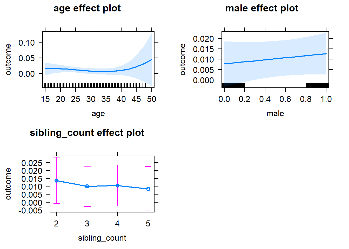
Add Birth Order Linear
Model Summary
tidy(m2_birthorder_linear, conf.int = T, conf.level = 0.995)| effect | group | term | estimate | std.error | statistic | df | p.value | conf.low | conf.high |
|---|---|---|---|---|---|---|---|---|---|
| fixed | NA | (Intercept) | -0.0374 | 0.09035 | -0.4139 | 2530 | 0.679 | -0.291 | 0.2162 |
| fixed | NA | birth_order | 0.0002983 | 0.002103 | 0.1419 | 2530 | 0.8872 | -0.005604 | 0.006201 |
| fixed | NA | poly(age, 3, raw = TRUE)1 | 0.007227 | 0.01001 | 0.722 | 2530 | 0.4704 | -0.02087 | 0.03533 |
| fixed | NA | poly(age, 3, raw = TRUE)2 | -0.0003096 | 0.0003549 | -0.8722 | 2530 | 0.3832 | -0.001306 | 0.0006867 |
| fixed | NA | poly(age, 3, raw = TRUE)3 | 0.000003958 | 0.000004031 | 0.982 | 2530 | 0.3262 | -0.000007357 | 0.00001527 |
| fixed | NA | male | 0.004927 | 0.004289 | 1.149 | 2530 | 0.2508 | -0.007114 | 0.01697 |
| fixed | NA | sibling_count3 | -0.003881 | 0.006257 | -0.6202 | 2530 | 0.5352 | -0.02145 | 0.01368 |
| fixed | NA | sibling_count4 | -0.003405 | 0.006546 | -0.5201 | 2530 | 0.603 | -0.02178 | 0.01497 |
| fixed | NA | sibling_count5 | -0.005717 | 0.007363 | -0.7765 | 2530 | 0.4376 | -0.02638 | 0.01495 |
| ran_pars | mother_pidlink | sd__(Intercept) | 0.000000001836 | NA | NA | NA | NA | NA | NA |
| ran_pars | Residual | sd__Observation | 0.1063 | NA | NA | NA | NA | NA | NA |
Coefficient Plot
plot_birthorder2(m2_birthorder_linear, separate = FALSE)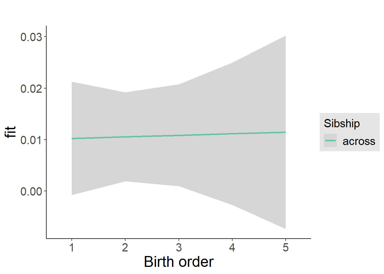
Add Birth Order Factor
Model Summary
m3_birthorder_nonlinear = update(m1_covariates_only, formula = . ~ . + birth_order_nonlinear)## boundary (singular) fit: see ?isSingulartidy(m3_birthorder_nonlinear, conf.int = T, conf.level = 0.995)| effect | group | term | estimate | std.error | statistic | df | p.value | conf.low | conf.high |
|---|---|---|---|---|---|---|---|---|---|
| fixed | NA | (Intercept) | -0.0304 | 0.09053 | -0.3358 | 2527 | 0.737 | -0.2845 | 0.2237 |
| fixed | NA | poly(age, 3, raw = TRUE)1 | 0.006574 | 0.01003 | 0.6553 | 2527 | 0.5124 | -0.02159 | 0.03473 |
| fixed | NA | poly(age, 3, raw = TRUE)2 | -0.0002858 | 0.0003557 | -0.8035 | 2527 | 0.4218 | -0.001284 | 0.0007126 |
| fixed | NA | poly(age, 3, raw = TRUE)3 | 0.000003693 | 0.000004039 | 0.9144 | 2527 | 0.3606 | -0.000007645 | 0.00001503 |
| fixed | NA | male | 0.004788 | 0.004292 | 1.116 | 2527 | 0.2647 | -0.00726 | 0.01684 |
| fixed | NA | sibling_count3 | -0.002776 | 0.006358 | -0.4366 | 2527 | 0.6624 | -0.02062 | 0.01507 |
| fixed | NA | sibling_count4 | -0.003536 | 0.006636 | -0.5328 | 2527 | 0.5942 | -0.02216 | 0.01509 |
| fixed | NA | sibling_count5 | -0.006162 | 0.007414 | -0.8311 | 2527 | 0.406 | -0.02697 | 0.01465 |
| fixed | NA | birth_order_nonlinear2 | -0.002972 | 0.005195 | -0.5722 | 2527 | 0.5673 | -0.01755 | 0.01161 |
| fixed | NA | birth_order_nonlinear3 | -0.004341 | 0.006384 | -0.6799 | 2527 | 0.4967 | -0.02226 | 0.01358 |
| fixed | NA | birth_order_nonlinear4 | 0.006187 | 0.00835 | 0.741 | 2527 | 0.4588 | -0.01725 | 0.02963 |
| fixed | NA | birth_order_nonlinear5 | 0.0006858 | 0.01196 | 0.05733 | 2527 | 0.9543 | -0.03289 | 0.03426 |
| ran_pars | mother_pidlink | sd__(Intercept) | 0.000000001149 | NA | NA | NA | NA | NA | NA |
| ran_pars | Residual | sd__Observation | 0.1064 | NA | NA | NA | NA | NA | NA |
Coefficient Plot
plot_birthorder(m3_birthorder_nonlinear, separate = FALSE)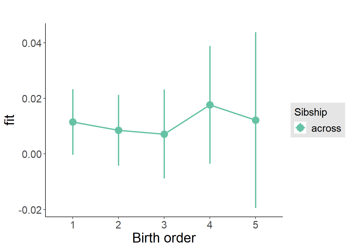
Add Interaction
Model Summary
m4_interaction = update(m3_birthorder_nonlinear, formula = . ~ . - birth_order_nonlinear - sibling_count + count_birth_order)## boundary (singular) fit: see ?isSingulartidy(m4_interaction, conf.int = T, conf.level = 0.995)| effect | group | term | estimate | std.error | statistic | df | p.value | conf.low | conf.high |
|---|---|---|---|---|---|---|---|---|---|
| fixed | NA | (Intercept) | -0.03185 | 0.09066 | -0.3513 | 2521 | 0.7254 | -0.2863 | 0.2226 |
| fixed | NA | poly(age, 3, raw = TRUE)1 | 0.006789 | 0.01005 | 0.6759 | 2521 | 0.4992 | -0.02141 | 0.03499 |
| fixed | NA | poly(age, 3, raw = TRUE)2 | -0.0002919 | 0.0003562 | -0.8196 | 2521 | 0.4125 | -0.001292 | 0.0007079 |
| fixed | NA | poly(age, 3, raw = TRUE)3 | 0.000003742 | 0.000004045 | 0.9252 | 2521 | 0.3549 | -0.000007611 | 0.0000151 |
| fixed | NA | male | 0.00488 | 0.004303 | 1.134 | 2521 | 0.2568 | -0.007198 | 0.01696 |
| fixed | NA | count_birth_order2/2 | -0.005527 | 0.009966 | -0.5546 | 2521 | 0.5792 | -0.0335 | 0.02245 |
| fixed | NA | count_birth_order1/3 | -0.007423 | 0.008344 | -0.8895 | 2521 | 0.3738 | -0.03085 | 0.016 |
| fixed | NA | count_birth_order2/3 | -0.00799 | 0.009079 | -0.88 | 2521 | 0.3789 | -0.03347 | 0.0175 |
| fixed | NA | count_birth_order3/3 | 0.0009479 | 0.009994 | 0.09485 | 2521 | 0.9244 | -0.02711 | 0.029 |
| fixed | NA | count_birth_order1/4 | 0.0007023 | 0.009102 | 0.07716 | 2521 | 0.9385 | -0.02485 | 0.02625 |
| fixed | NA | count_birth_order2/4 | -0.006345 | 0.009498 | -0.668 | 2521 | 0.5042 | -0.03301 | 0.02032 |
| fixed | NA | count_birth_order3/4 | -0.01548 | 0.01039 | -1.49 | 2521 | 0.1363 | -0.04465 | 0.01368 |
| fixed | NA | count_birth_order4/4 | -0.0009842 | 0.01108 | -0.08884 | 2521 | 0.9292 | -0.03208 | 0.03011 |
| fixed | NA | count_birth_order1/5 | -0.009076 | 0.01093 | -0.83 | 2521 | 0.4066 | -0.03977 | 0.02162 |
| fixed | NA | count_birth_order2/5 | -0.006608 | 0.01136 | -0.5819 | 2521 | 0.5607 | -0.03849 | 0.02527 |
| fixed | NA | count_birth_order3/5 | -0.01542 | 0.01156 | -1.334 | 2521 | 0.1823 | -0.04786 | 0.01702 |
| fixed | NA | count_birth_order4/5 | 0.0024 | 0.01173 | 0.2045 | 2521 | 0.838 | -0.03054 | 0.03534 |
| fixed | NA | count_birth_order5/5 | -0.006338 | 0.01183 | -0.5359 | 2521 | 0.5921 | -0.03953 | 0.02686 |
| ran_pars | mother_pidlink | sd__(Intercept) | 0 | NA | NA | NA | NA | NA | NA |
| ran_pars | Residual | sd__Observation | 0.1064 | NA | NA | NA | NA | NA | NA |
Coefficient Plot
plot_birthorder(m4_interaction)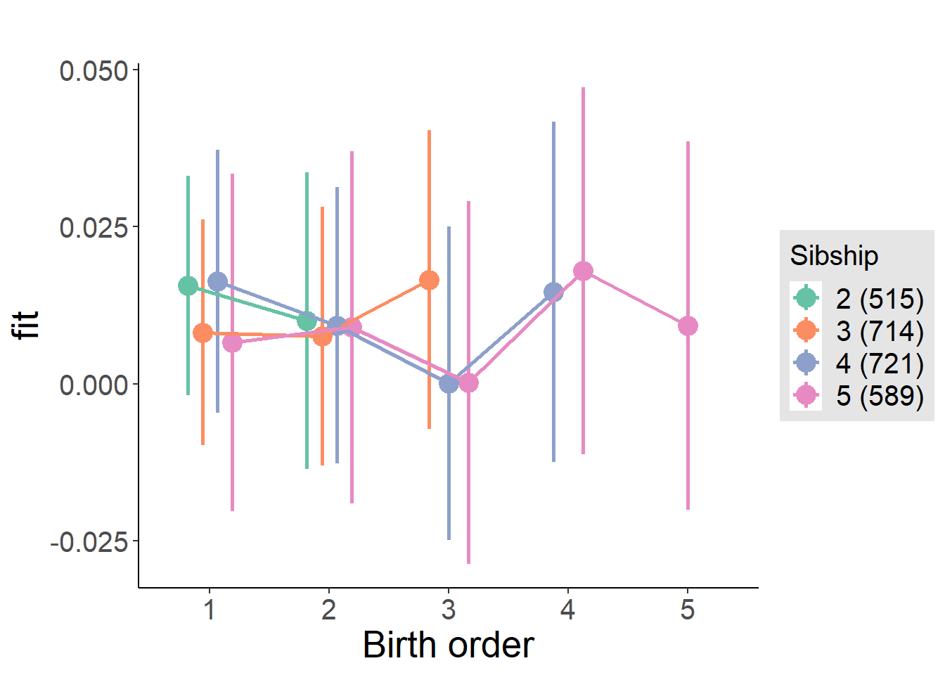
Model Comparison
###### Model 1 - Model 2
anova(m1_covariates_only, m2_birthorder_linear, m3_birthorder_nonlinear, m4_interaction)## refitting model(s) with ML (instead of REML)| Df | AIC | BIC | logLik | deviance | Chisq | Chi Df | Pr(>Chisq) |
|---|---|---|---|---|---|---|---|
| 10 | -4165 | -4106 | 2092 | -4185 | NA | NA | NA |
| 11 | -4163 | -4098 | 2092 | -4185 | 0.02019 | 1 | 0.887 |
| 14 | -4158 | -4077 | 2093 | -4186 | 1.75 | 3 | 0.6258 |
| 20 | -4150 | -4033 | 2095 | -4190 | 3.425 | 6 | 0.7539 |
Parental full sibling order
outcome_parental_m1 <- update(m2_birthorder_linear, data = birthorder %>%
mutate(sibling_count = sibling_count_genes_factor,
birth_order_nonlinear = birthorder_genes_factor,
birth_order = birthorder_genes,
count_birth_order = count_birthorder_genes
) %>%
filter(sibling_count != "1"))
compare_models_markdown(outcome_parental_m1)Basic Model
Model Summary
m1_covariates_only <- update(m2_birthorder_linear, formula = . ~ . - birth_order)
tidy(m1_covariates_only, conf.int = T, conf.level = 0.995)| effect | group | term | estimate | std.error | statistic | df | p.value | conf.low | conf.high |
|---|---|---|---|---|---|---|---|---|---|
| fixed | NA | (Intercept) | -0.09021 | 0.08585 | -1.051 | 2758 | 0.2934 | -0.3312 | 0.1508 |
| fixed | NA | poly(age, 3, raw = TRUE)1 | 0.01283 | 0.009534 | 1.346 | 2759 | 0.1784 | -0.01393 | 0.0396 |
| fixed | NA | poly(age, 3, raw = TRUE)2 | -0.0005036 | 0.0003389 | -1.486 | 2759 | 0.1374 | -0.001455 | 0.0004477 |
| fixed | NA | poly(age, 3, raw = TRUE)3 | 0.000006072 | 0.000003859 | 1.573 | 2759 | 0.1158 | -0.000004761 | 0.0000169 |
| fixed | NA | male | 0.004031 | 0.00397 | 1.015 | 2687 | 0.31 | -0.007112 | 0.01517 |
| fixed | NA | sibling_count3 | -0.003783 | 0.005536 | -0.6832 | 1937 | 0.4945 | -0.01932 | 0.01176 |
| fixed | NA | sibling_count4 | 0.002987 | 0.005832 | 0.5122 | 1755 | 0.6086 | -0.01338 | 0.01936 |
| fixed | NA | sibling_count5 | 0.0001261 | 0.006691 | 0.01884 | 1443 | 0.985 | -0.01866 | 0.01891 |
| ran_pars | mother_pidlink | sd__(Intercept) | 0.0426 | NA | NA | NA | NA | NA | NA |
| ran_pars | Residual | sd__Observation | 0.0946 | NA | NA | NA | NA | NA | NA |
Coefficient Plot
plot(allEffects(m1_covariates_only, confidence.level = 0.995))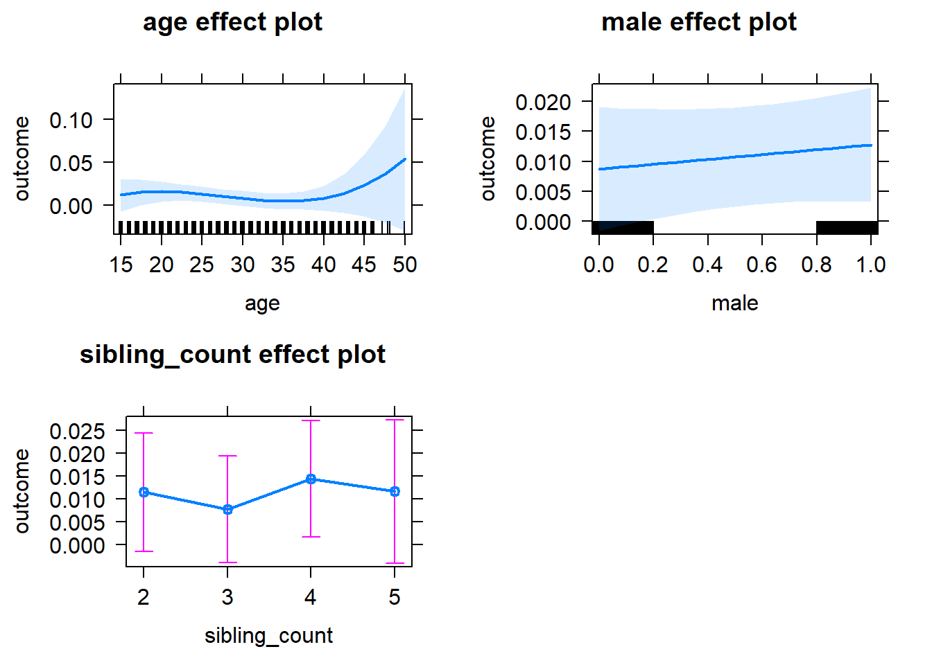
Add Birth Order Linear
Model Summary
tidy(m2_birthorder_linear, conf.int = T, conf.level = 0.995)| effect | group | term | estimate | std.error | statistic | df | p.value | conf.low | conf.high |
|---|---|---|---|---|---|---|---|---|---|
| fixed | NA | (Intercept) | -0.0903 | 0.08587 | -1.052 | 2757 | 0.2931 | -0.3313 | 0.1507 |
| fixed | NA | birth_order | 0.000237 | 0.002013 | 0.1177 | 2439 | 0.9063 | -0.005414 | 0.005888 |
| fixed | NA | poly(age, 3, raw = TRUE)1 | 0.01281 | 0.009537 | 1.344 | 2758 | 0.1792 | -0.01396 | 0.03958 |
| fixed | NA | poly(age, 3, raw = TRUE)2 | -0.0005033 | 0.000339 | -1.485 | 2758 | 0.1377 | -0.001455 | 0.0004482 |
| fixed | NA | poly(age, 3, raw = TRUE)3 | 0.000006075 | 0.00000386 | 1.574 | 2758 | 0.1157 | -0.00000476 | 0.00001691 |
| fixed | NA | male | 0.004033 | 0.003971 | 1.016 | 2686 | 0.3099 | -0.007113 | 0.01518 |
| fixed | NA | sibling_count3 | -0.003899 | 0.005625 | -0.6931 | 1975 | 0.4883 | -0.01969 | 0.01189 |
| fixed | NA | sibling_count4 | 0.002745 | 0.006185 | 0.4438 | 1909 | 0.6572 | -0.01462 | 0.02011 |
| fixed | NA | sibling_count5 | -0.0002713 | 0.007497 | -0.03619 | 1770 | 0.9711 | -0.02132 | 0.02077 |
| ran_pars | mother_pidlink | sd__(Intercept) | 0.04257 | NA | NA | NA | NA | NA | NA |
| ran_pars | Residual | sd__Observation | 0.09464 | NA | NA | NA | NA | NA | NA |
Coefficient Plot
plot_birthorder2(m2_birthorder_linear, separate = FALSE)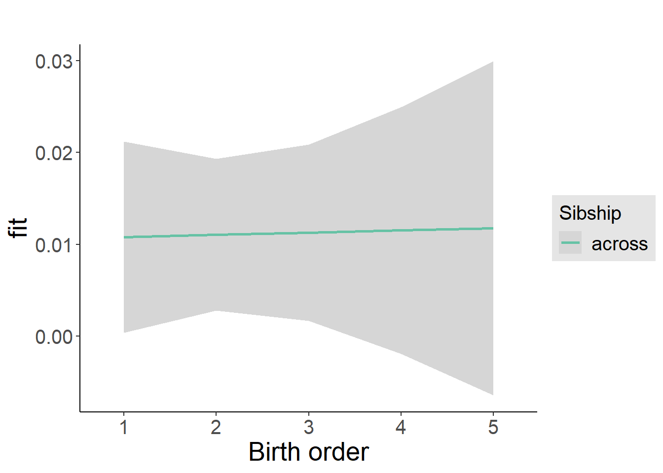
Add Birth Order Factor
Model Summary
m3_birthorder_nonlinear = update(m1_covariates_only, formula = . ~ . + birth_order_nonlinear)
tidy(m3_birthorder_nonlinear, conf.int = T, conf.level = 0.995)| effect | group | term | estimate | std.error | statistic | df | p.value | conf.low | conf.high |
|---|---|---|---|---|---|---|---|---|---|
| fixed | NA | (Intercept) | -0.08387 | 0.08599 | -0.9754 | 2753 | 0.3295 | -0.3252 | 0.1575 |
| fixed | NA | poly(age, 3, raw = TRUE)1 | 0.01218 | 0.009549 | 1.275 | 2754 | 0.2023 | -0.01463 | 0.03898 |
| fixed | NA | poly(age, 3, raw = TRUE)2 | -0.0004812 | 0.0003394 | -1.418 | 2754 | 0.1563 | -0.001434 | 0.0004714 |
| fixed | NA | poly(age, 3, raw = TRUE)3 | 0.00000584 | 0.000003864 | 1.511 | 2755 | 0.1309 | -0.000005008 | 0.00001669 |
| fixed | NA | male | 0.00386 | 0.003973 | 0.9714 | 2688 | 0.3314 | -0.007293 | 0.01501 |
| fixed | NA | sibling_count3 | -0.003168 | 0.005703 | -0.5555 | 2052 | 0.5786 | -0.01918 | 0.01284 |
| fixed | NA | sibling_count4 | 0.001371 | 0.006254 | 0.2192 | 1975 | 0.8265 | -0.01618 | 0.01893 |
| fixed | NA | sibling_count5 | 0.0000704 | 0.007605 | 0.009256 | 1830 | 0.9926 | -0.02128 | 0.02142 |
| fixed | NA | birth_order_nonlinear2 | -0.001232 | 0.004682 | -0.2631 | 2069 | 0.7925 | -0.01437 | 0.01191 |
| fixed | NA | birth_order_nonlinear3 | -0.002785 | 0.005769 | -0.4827 | 2167 | 0.6294 | -0.01898 | 0.01341 |
| fixed | NA | birth_order_nonlinear4 | 0.01128 | 0.0079 | 1.428 | 2250 | 0.1534 | -0.01089 | 0.03346 |
| fixed | NA | birth_order_nonlinear5 | -0.01121 | 0.01244 | -0.9008 | 2165 | 0.3678 | -0.04614 | 0.02372 |
| ran_pars | mother_pidlink | sd__(Intercept) | 0.04195 | NA | NA | NA | NA | NA | NA |
| ran_pars | Residual | sd__Observation | 0.09485 | NA | NA | NA | NA | NA | NA |
Coefficient Plot
plot_birthorder(m3_birthorder_nonlinear, separate = FALSE)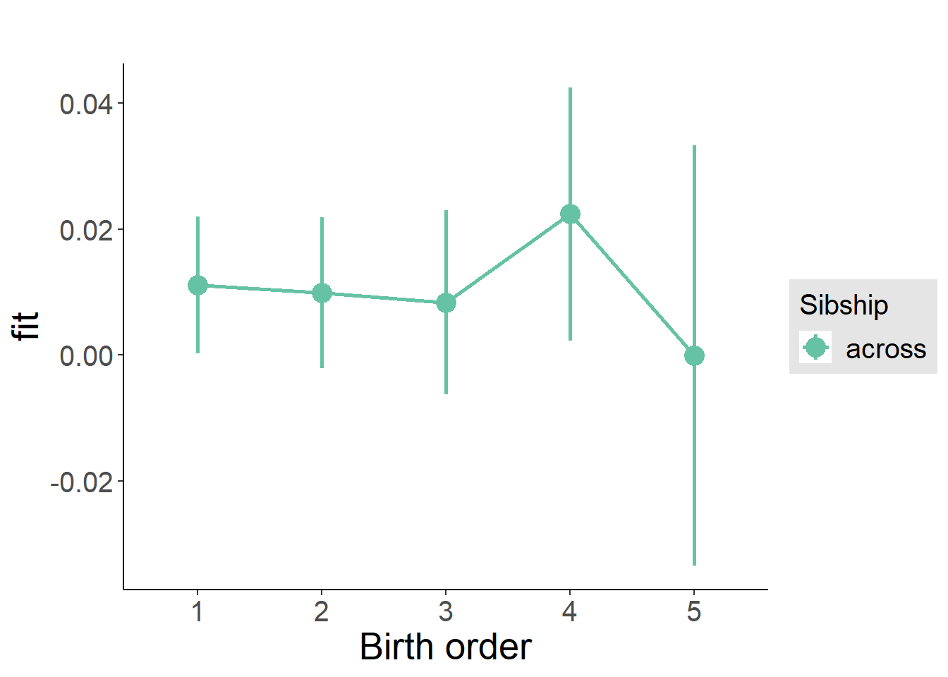
Add Interaction
Model Summary
m4_interaction = update(m3_birthorder_nonlinear, formula = . ~ . - birth_order_nonlinear - sibling_count + count_birth_order)
tidy(m4_interaction, conf.int = T, conf.level = 0.995)| effect | group | term | estimate | std.error | statistic | df | p.value | conf.low | conf.high |
|---|---|---|---|---|---|---|---|---|---|
| fixed | NA | (Intercept) | -0.08567 | 0.08604 | -0.9957 | 2747 | 0.3195 | -0.3272 | 0.1558 |
| fixed | NA | poly(age, 3, raw = TRUE)1 | 0.01254 | 0.009555 | 1.312 | 2748 | 0.1895 | -0.01428 | 0.03936 |
| fixed | NA | poly(age, 3, raw = TRUE)2 | -0.0004935 | 0.0003396 | -1.453 | 2749 | 0.1463 | -0.001447 | 0.0004598 |
| fixed | NA | poly(age, 3, raw = TRUE)3 | 0.000005969 | 0.000003868 | 1.543 | 2749 | 0.1229 | -0.000004889 | 0.00001683 |
| fixed | NA | male | 0.00391 | 0.003977 | 0.9831 | 2680 | 0.3257 | -0.007255 | 0.01507 |
| fixed | NA | count_birth_order2/2 | -0.005724 | 0.008349 | -0.6857 | 2156 | 0.493 | -0.02916 | 0.01771 |
| fixed | NA | count_birth_order1/3 | -0.008734 | 0.007213 | -1.211 | 2741 | 0.226 | -0.02898 | 0.01151 |
| fixed | NA | count_birth_order2/3 | -0.00658 | 0.008011 | -0.8214 | 2748 | 0.4115 | -0.02907 | 0.01591 |
| fixed | NA | count_birth_order3/3 | 0.001169 | 0.008572 | 0.1364 | 2738 | 0.8915 | -0.02289 | 0.02523 |
| fixed | NA | count_birth_order1/4 | 0.005607 | 0.008477 | 0.6614 | 2750 | 0.5084 | -0.01819 | 0.0294 |
| fixed | NA | count_birth_order2/4 | 0.002235 | 0.008838 | 0.2529 | 2742 | 0.8004 | -0.02257 | 0.02704 |
| fixed | NA | count_birth_order3/4 | -0.01064 | 0.009256 | -1.15 | 2724 | 0.2502 | -0.03663 | 0.01534 |
| fixed | NA | count_birth_order4/4 | 0.006129 | 0.009971 | 0.6147 | 2717 | 0.5388 | -0.02186 | 0.03412 |
| fixed | NA | count_birth_order1/5 | -0.004282 | 0.01111 | -0.3855 | 2746 | 0.6999 | -0.03546 | 0.0269 |
| fixed | NA | count_birth_order2/5 | -0.0007552 | 0.01242 | -0.06081 | 2681 | 0.9515 | -0.03562 | 0.03411 |
| fixed | NA | count_birth_order3/5 | -0.00937 | 0.01188 | -0.7889 | 2685 | 0.4302 | -0.04271 | 0.02397 |
| fixed | NA | count_birth_order4/5 | 0.01664 | 0.01144 | 1.454 | 2691 | 0.1462 | -0.01549 | 0.04876 |
| fixed | NA | count_birth_order5/5 | -0.01257 | 0.01204 | -1.043 | 2680 | 0.2968 | -0.04637 | 0.02124 |
| ran_pars | mother_pidlink | sd__(Intercept) | 0.04206 | NA | NA | NA | NA | NA | NA |
| ran_pars | Residual | sd__Observation | 0.09482 | NA | NA | NA | NA | NA | NA |
Coefficient Plot
plot_birthorder(m4_interaction)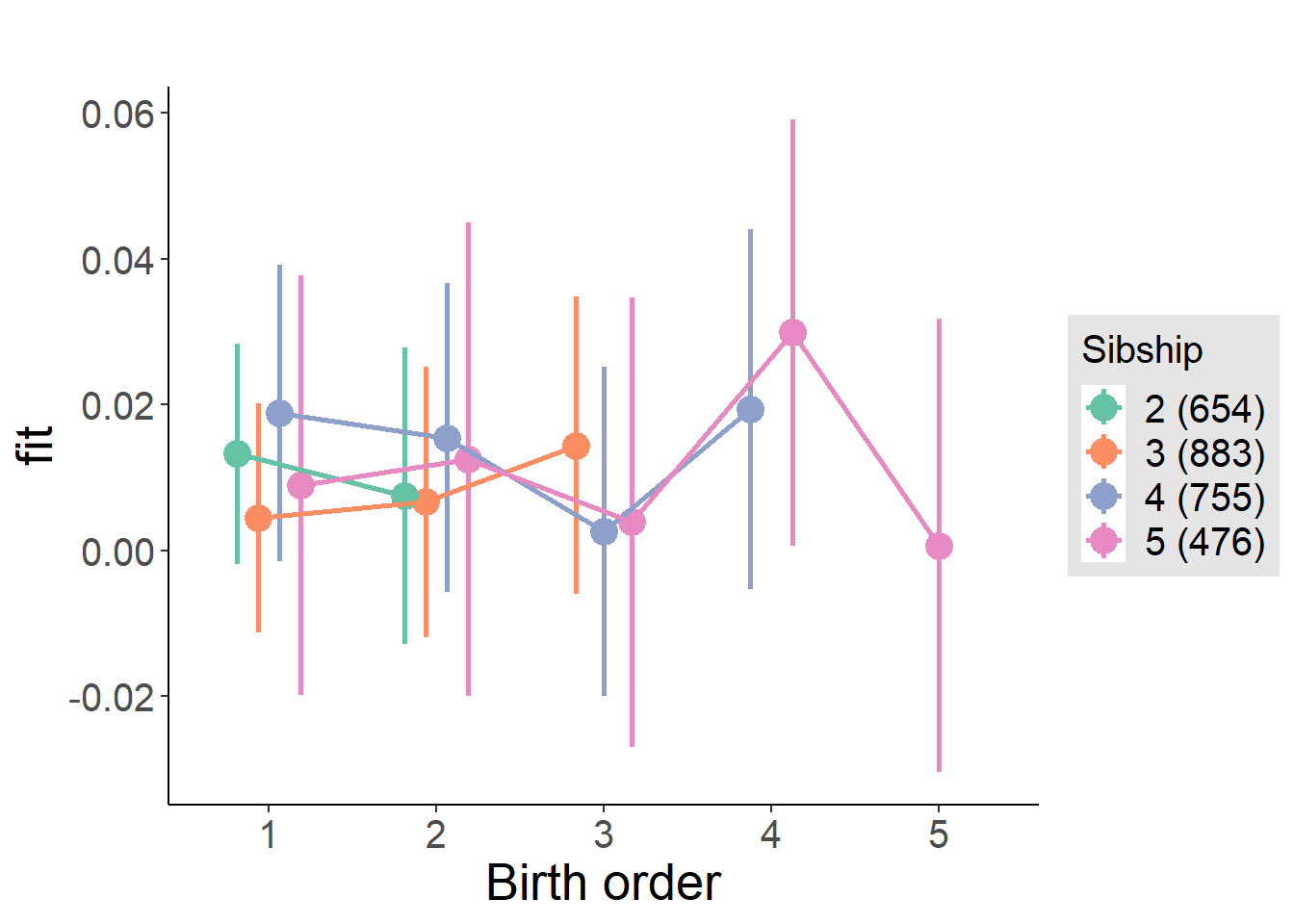
Model Comparison
###### Model 1 - Model 2
anova(m1_covariates_only, m2_birthorder_linear, m3_birthorder_nonlinear, m4_interaction)## refitting model(s) with ML (instead of REML)| Df | AIC | BIC | logLik | deviance | Chisq | Chi Df | Pr(>Chisq) |
|---|---|---|---|---|---|---|---|
| 10 | -4701 | -4642 | 2361 | -4721 | NA | NA | NA |
| 11 | -4699 | -4634 | 2361 | -4721 | 0.01415 | 1 | 0.9053 |
| 14 | -4697 | -4614 | 2363 | -4725 | 4.415 | 3 | 0.22 |
| 20 | -4691 | -4573 | 2366 | -4731 | 5.766 | 6 | 0.4499 |
Compare birth order specifications
library(coefplot)
multiplot(outcome_naive_m1, outcome_preg_m1, outcome_uterus_m1, outcome_parental_m1, dodgeHeight = 0.6,
intercept = FALSE)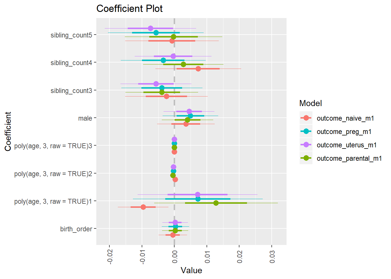
Category_Casual worker not in agriculture
birthorder <- birthorder %>% mutate(outcome = `Category_Casual worker not in agriculture`)
model = lmer(outcome ~ birth_order + poly(age, 3, raw = TRUE) + male + sibling_count + (1 | mother_pidlink),
data = birthorder)
compare_birthorder_specs(model)Naive birth order
outcome_naive_m1 <- update(m2_birthorder_linear, data = birthorder %>%
mutate(sibling_count = sibling_count_naive_factor,
birth_order_nonlinear = birthorder_naive_factor,
birth_order = birthorder_naive,
count_birth_order = count_birthorder_naive) %>%
filter(sibling_count != "1"))
compare_models_markdown(outcome_naive_m1)Basic Model
Model Summary
m1_covariates_only <- update(m2_birthorder_linear, formula = . ~ . - birth_order)
tidy(m1_covariates_only, conf.int = T, conf.level = 0.995)| effect | group | term | estimate | std.error | statistic | df | p.value | conf.low | conf.high |
|---|---|---|---|---|---|---|---|---|---|
| fixed | NA | (Intercept) | 0.304 | 0.07921 | 3.838 | 4453 | 0.0001256 | 0.08169 | 0.5264 |
| fixed | NA | poly(age, 3, raw = TRUE)1 | -0.02036 | 0.007068 | -2.88 | 4340 | 0.003998 | -0.0402 | -0.0005148 |
| fixed | NA | poly(age, 3, raw = TRUE)2 | 0.0004827 | 0.0001963 | 2.458 | 4206 | 0.01399 | -0.00006844 | 0.001034 |
| fixed | NA | poly(age, 3, raw = TRUE)3 | -0.000003481 | 0.000001717 | -2.027 | 4085 | 0.04275 | -0.000008302 | 0.00000134 |
| fixed | NA | male | 0.06724 | 0.00801 | 8.394 | 4744 | 6.134e-17 | 0.04475 | 0.08972 |
| fixed | NA | sibling_count3 | 0.002986 | 0.01163 | 0.2568 | 3381 | 0.7973 | -0.02965 | 0.03562 |
| fixed | NA | sibling_count4 | -0.00636 | 0.01176 | -0.5408 | 3166 | 0.5887 | -0.03937 | 0.02665 |
| fixed | NA | sibling_count5 | -0.0005289 | 0.01228 | -0.04307 | 2937 | 0.9656 | -0.035 | 0.03394 |
| ran_pars | mother_pidlink | sd__(Intercept) | 0.1018 | NA | NA | NA | NA | NA | NA |
| ran_pars | Residual | sd__Observation | 0.2578 | NA | NA | NA | NA | NA | NA |
Coefficient Plot
plot(allEffects(m1_covariates_only, confidence.level = 0.995))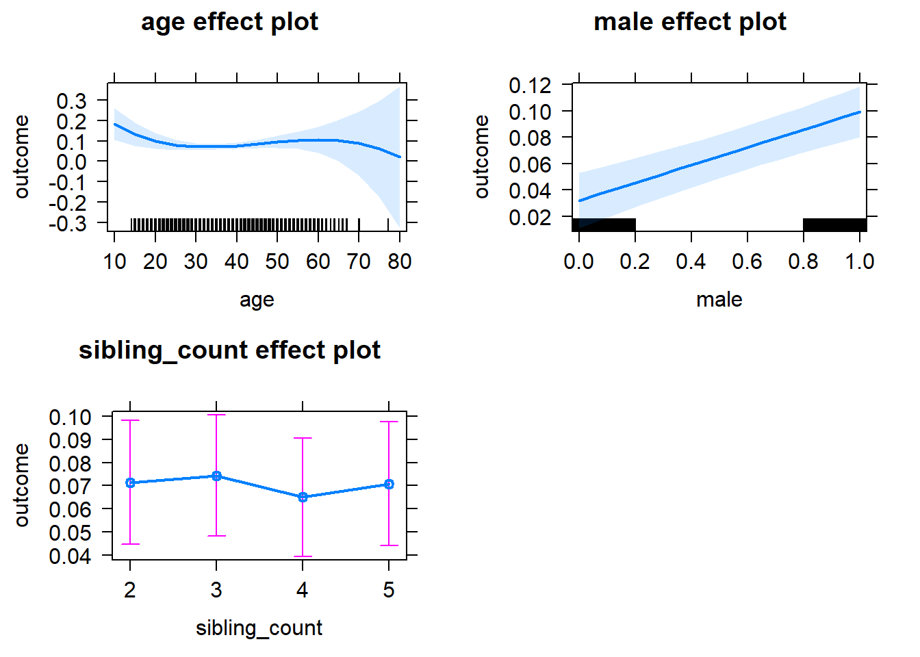
Add Birth Order Linear
Model Summary
tidy(m2_birthorder_linear, conf.int = T, conf.level = 0.995)| effect | group | term | estimate | std.error | statistic | df | p.value | conf.low | conf.high |
|---|---|---|---|---|---|---|---|---|---|
| fixed | NA | (Intercept) | 0.3047 | 0.07921 | 3.847 | 4452 | 0.0001212 | 0.08238 | 0.5271 |
| fixed | NA | birth_order | 0.003714 | 0.003919 | 0.9476 | 4170 | 0.3434 | -0.007288 | 0.01471 |
| fixed | NA | poly(age, 3, raw = TRUE)1 | -0.02091 | 0.007092 | -2.949 | 4340 | 0.003209 | -0.04082 | -0.001004 |
| fixed | NA | poly(age, 3, raw = TRUE)2 | 0.0004968 | 0.0001969 | 2.523 | 4197 | 0.01167 | -0.00005588 | 0.001049 |
| fixed | NA | poly(age, 3, raw = TRUE)3 | -0.000003576 | 0.00000172 | -2.079 | 4077 | 0.03769 | -0.000008405 | 0.000001253 |
| fixed | NA | male | 0.06727 | 0.00801 | 8.398 | 4743 | 5.924e-17 | 0.04479 | 0.08976 |
| fixed | NA | sibling_count3 | 0.001585 | 0.01172 | 0.1352 | 3471 | 0.8924 | -0.03131 | 0.03448 |
| fixed | NA | sibling_count4 | -0.009337 | 0.01217 | -0.767 | 3526 | 0.4431 | -0.04351 | 0.02483 |
| fixed | NA | sibling_count5 | -0.005293 | 0.01327 | -0.3989 | 3658 | 0.69 | -0.04254 | 0.03195 |
| ran_pars | mother_pidlink | sd__(Intercept) | 0.1017 | NA | NA | NA | NA | NA | NA |
| ran_pars | Residual | sd__Observation | 0.2578 | NA | NA | NA | NA | NA | NA |
Coefficient Plot
plot_birthorder2(m2_birthorder_linear, separate = FALSE)
Add Birth Order Factor
Model Summary
m3_birthorder_nonlinear = update(m1_covariates_only, formula = . ~ . + birth_order_nonlinear)
tidy(m3_birthorder_nonlinear, conf.int = T, conf.level = 0.995)| effect | group | term | estimate | std.error | statistic | df | p.value | conf.low | conf.high |
|---|---|---|---|---|---|---|---|---|---|
| fixed | NA | (Intercept) | 0.3076 | 0.07944 | 3.873 | 4455 | 0.0001092 | 0.08465 | 0.5306 |
| fixed | NA | poly(age, 3, raw = TRUE)1 | -0.02093 | 0.007094 | -2.95 | 4332 | 0.003199 | -0.04084 | -0.001012 |
| fixed | NA | poly(age, 3, raw = TRUE)2 | 0.000494 | 0.000197 | 2.508 | 4184 | 0.01219 | -0.00005899 | 0.001047 |
| fixed | NA | poly(age, 3, raw = TRUE)3 | -0.000003523 | 0.000001722 | -2.046 | 4056 | 0.0408 | -0.000008357 | 0.00000131 |
| fixed | NA | male | 0.06714 | 0.008015 | 8.377 | 4741 | 7.089e-17 | 0.04464 | 0.08964 |
| fixed | NA | sibling_count3 | -0.0001352 | 0.01191 | -0.01135 | 3626 | 0.9909 | -0.03357 | 0.0333 |
| fixed | NA | sibling_count4 | -0.01053 | 0.01238 | -0.8511 | 3687 | 0.3948 | -0.04527 | 0.02421 |
| fixed | NA | sibling_count5 | -0.003783 | 0.01339 | -0.2825 | 3755 | 0.7776 | -0.04137 | 0.0338 |
| fixed | NA | birth_order_nonlinear2 | 0.009483 | 0.009451 | 1.003 | 4087 | 0.3157 | -0.01705 | 0.03601 |
| fixed | NA | birth_order_nonlinear3 | 0.01615 | 0.01202 | 1.343 | 4013 | 0.1792 | -0.01759 | 0.04989 |
| fixed | NA | birth_order_nonlinear4 | 0.01101 | 0.01561 | 0.7055 | 3968 | 0.4806 | -0.0328 | 0.05482 |
| fixed | NA | birth_order_nonlinear5 | 0.00158 | 0.02255 | 0.07007 | 3979 | 0.9441 | -0.06171 | 0.06487 |
| ran_pars | mother_pidlink | sd__(Intercept) | 0.1013 | NA | NA | NA | NA | NA | NA |
| ran_pars | Residual | sd__Observation | 0.258 | NA | NA | NA | NA | NA | NA |
Coefficient Plot
plot_birthorder(m3_birthorder_nonlinear, separate = FALSE)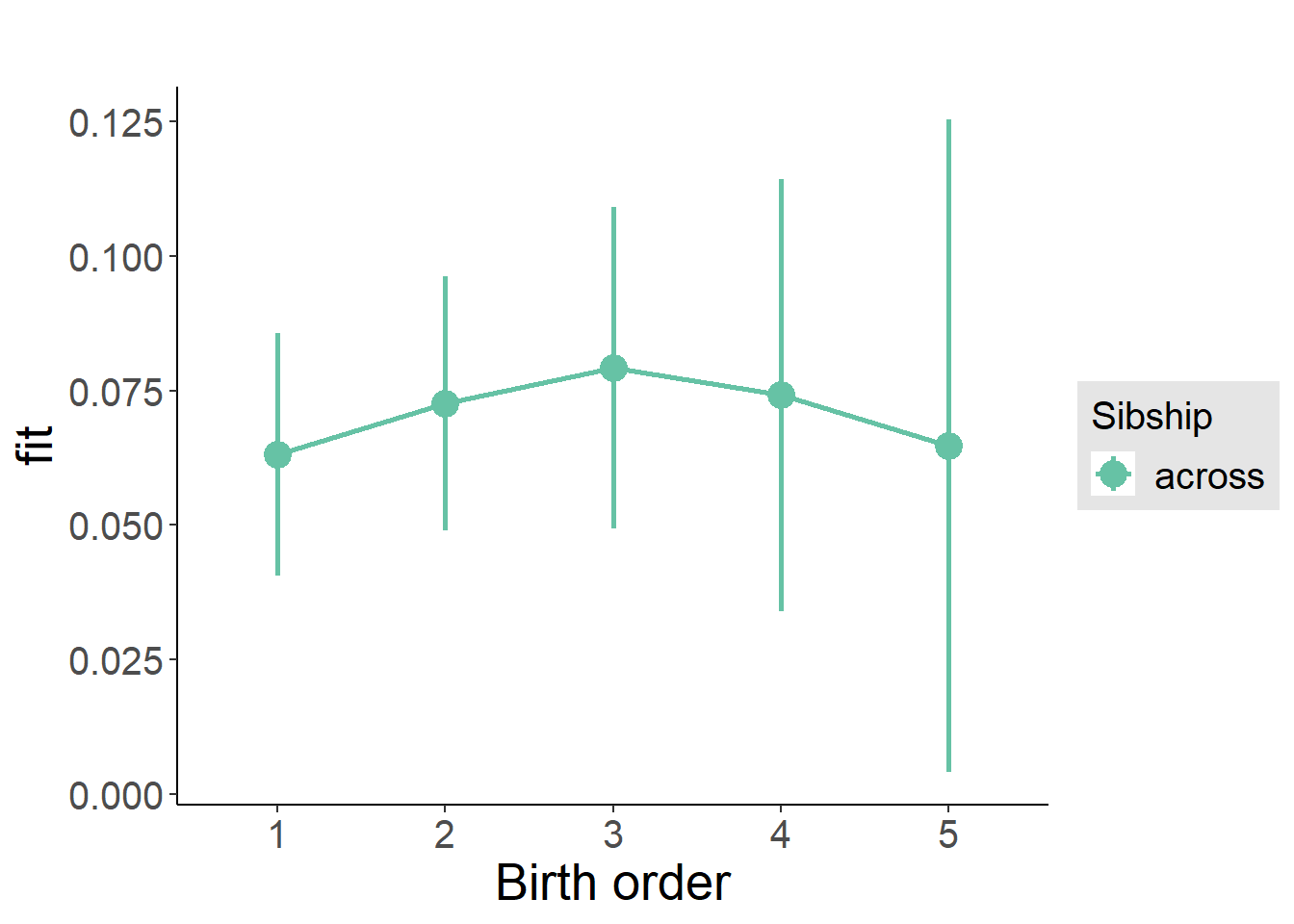
Add Interaction
Model Summary
m4_interaction = update(m3_birthorder_nonlinear, formula = . ~ . - birth_order_nonlinear - sibling_count + count_birth_order)
tidy(m4_interaction, conf.int = T, conf.level = 0.995)| effect | group | term | estimate | std.error | statistic | df | p.value | conf.low | conf.high |
|---|---|---|---|---|---|---|---|---|---|
| fixed | NA | (Intercept) | 0.3013 | 0.07955 | 3.787 | 4460 | 0.0001544 | 0.07797 | 0.5246 |
| fixed | NA | poly(age, 3, raw = TRUE)1 | -0.02035 | 0.007099 | -2.866 | 4330 | 0.004177 | -0.04027 | -0.0004183 |
| fixed | NA | poly(age, 3, raw = TRUE)2 | 0.0004822 | 0.0001971 | 2.447 | 4181 | 0.01444 | -0.00007094 | 0.001035 |
| fixed | NA | poly(age, 3, raw = TRUE)3 | -0.000003464 | 0.000001722 | -2.011 | 4053 | 0.04434 | -0.000008299 | 0.00000137 |
| fixed | NA | male | 0.06747 | 0.008017 | 8.415 | 4733 | 5.126e-17 | 0.04496 | 0.08997 |
| fixed | NA | count_birth_order2/2 | 0.005435 | 0.01605 | 0.3386 | 4038 | 0.7349 | -0.03962 | 0.05049 |
| fixed | NA | count_birth_order1/3 | 0.0087 | 0.01556 | 0.5591 | 4791 | 0.5762 | -0.03499 | 0.05239 |
| fixed | NA | count_birth_order2/3 | 0.008848 | 0.01726 | 0.5126 | 4804 | 0.6082 | -0.0396 | 0.05729 |
| fixed | NA | count_birth_order3/3 | -0.006577 | 0.01899 | -0.3464 | 4806 | 0.7291 | -0.05988 | 0.04672 |
| fixed | NA | count_birth_order1/4 | -0.02392 | 0.01706 | -1.402 | 4804 | 0.1609 | -0.07181 | 0.02397 |
| fixed | NA | count_birth_order2/4 | 0.008356 | 0.0183 | 0.4567 | 4806 | 0.6479 | -0.043 | 0.05972 |
| fixed | NA | count_birth_order3/4 | 0.01317 | 0.01952 | 0.6746 | 4804 | 0.5 | -0.04162 | 0.06795 |
| fixed | NA | count_birth_order4/4 | -0.007139 | 0.02076 | -0.3438 | 4802 | 0.731 | -0.06542 | 0.05115 |
| fixed | NA | count_birth_order1/5 | -0.01235 | 0.01937 | -0.6375 | 4804 | 0.5238 | -0.06671 | 0.04202 |
| fixed | NA | count_birth_order2/5 | -0.009084 | 0.02056 | -0.4419 | 4800 | 0.6586 | -0.06678 | 0.04862 |
| fixed | NA | count_birth_order3/5 | 0.0283 | 0.02164 | 1.308 | 4794 | 0.191 | -0.03244 | 0.08903 |
| fixed | NA | count_birth_order4/5 | 0.01301 | 0.02276 | 0.5718 | 4771 | 0.5675 | -0.05086 | 0.07688 |
| fixed | NA | count_birth_order5/5 | -0.003641 | 0.02277 | -0.1599 | 4788 | 0.873 | -0.06756 | 0.06028 |
| ran_pars | mother_pidlink | sd__(Intercept) | 0.1015 | NA | NA | NA | NA | NA | NA |
| ran_pars | Residual | sd__Observation | 0.2579 | NA | NA | NA | NA | NA | NA |
Coefficient Plot
plot_birthorder(m4_interaction)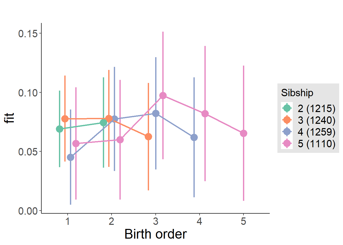
Model Comparison
###### Model 1 - Model 2
anova(m1_covariates_only, m2_birthorder_linear, m3_birthorder_nonlinear, m4_interaction)## refitting model(s) with ML (instead of REML)| Df | AIC | BIC | logLik | deviance | Chisq | Chi Df | Pr(>Chisq) |
|---|---|---|---|---|---|---|---|
| 10 | 1287 | 1352 | -633.7 | 1267 | NA | NA | NA |
| 11 | 1288 | 1360 | -633.2 | 1266 | 0.8999 | 1 | 0.3428 |
| 14 | 1293 | 1384 | -632.5 | 1265 | 1.379 | 3 | 0.7104 |
| 20 | 1299 | 1428 | -629.4 | 1259 | 6.29 | 6 | 0.3915 |
Maternal birth order
outcome_uterus_m1 <- update(m2_birthorder_linear, data = birthorder %>%
mutate(sibling_count = sibling_count_uterus_alive_factor,
birth_order_nonlinear = birthorder_uterus_alive_factor,
birth_order = birthorder_uterus_alive,
count_birth_order = count_birthorder_uterus_alive) %>%
filter(sibling_count != "1"))
compare_models_markdown(outcome_uterus_m1)Basic Model
Model Summary
m1_covariates_only <- update(m2_birthorder_linear, formula = . ~ . - birth_order)
tidy(m1_covariates_only, conf.int = T, conf.level = 0.995)| effect | group | term | estimate | std.error | statistic | df | p.value | conf.low | conf.high |
|---|---|---|---|---|---|---|---|---|---|
| fixed | NA | (Intercept) | 0.6334 | 0.2145 | 2.952 | 2750 | 0.003182 | 0.03115 | 1.236 |
| fixed | NA | poly(age, 3, raw = TRUE)1 | -0.0538 | 0.02377 | -2.264 | 2749 | 0.02367 | -0.1205 | 0.01291 |
| fixed | NA | poly(age, 3, raw = TRUE)2 | 0.00159 | 0.0008428 | 1.887 | 2748 | 0.05927 | -0.0007755 | 0.003956 |
| fixed | NA | poly(age, 3, raw = TRUE)3 | -0.00001566 | 0.000009572 | -1.636 | 2746 | 0.1019 | -0.00004253 | 0.00001121 |
| fixed | NA | male | 0.05029 | 0.01007 | 4.993 | 2749 | 0.0000006322 | 0.02201 | 0.07856 |
| fixed | NA | sibling_count3 | -0.005766 | 0.01403 | -0.4111 | 2122 | 0.6811 | -0.04514 | 0.03361 |
| fixed | NA | sibling_count4 | 0.008109 | 0.01453 | 0.558 | 1931 | 0.5769 | -0.03268 | 0.0489 |
| fixed | NA | sibling_count5 | -0.01658 | 0.01614 | -1.028 | 1654 | 0.3042 | -0.06187 | 0.02871 |
| ran_pars | mother_pidlink | sd__(Intercept) | 0.0734 | NA | NA | NA | NA | NA | NA |
| ran_pars | Residual | sd__Observation | 0.2509 | NA | NA | NA | NA | NA | NA |
Coefficient Plot
plot(allEffects(m1_covariates_only, confidence.level = 0.995))
Add Birth Order Linear
Model Summary
tidy(m2_birthorder_linear, conf.int = T, conf.level = 0.995)| effect | group | term | estimate | std.error | statistic | df | p.value | conf.low | conf.high |
|---|---|---|---|---|---|---|---|---|---|
| fixed | NA | (Intercept) | 0.6331 | 0.2146 | 2.95 | 2749 | 0.003205 | 0.03068 | 1.235 |
| fixed | NA | birth_order | 0.0006341 | 0.005075 | 0.125 | 2610 | 0.9006 | -0.01361 | 0.01488 |
| fixed | NA | poly(age, 3, raw = TRUE)1 | -0.05384 | 0.02377 | -2.265 | 2748 | 0.02361 | -0.1206 | 0.01289 |
| fixed | NA | poly(age, 3, raw = TRUE)2 | 0.001591 | 0.000843 | 1.887 | 2747 | 0.05926 | -0.0007756 | 0.003957 |
| fixed | NA | poly(age, 3, raw = TRUE)3 | -0.00001565 | 0.000009575 | -1.634 | 2745 | 0.1023 | -0.00004252 | 0.00001123 |
| fixed | NA | male | 0.05029 | 0.01007 | 4.992 | 2748 | 0.0000006345 | 0.02201 | 0.07856 |
| fixed | NA | sibling_count3 | -0.006071 | 0.01424 | -0.4263 | 2157 | 0.6699 | -0.04605 | 0.0339 |
| fixed | NA | sibling_count4 | 0.007458 | 0.01544 | 0.483 | 2070 | 0.6291 | -0.03588 | 0.0508 |
| fixed | NA | sibling_count5 | -0.01768 | 0.01836 | -0.9627 | 2003 | 0.3358 | -0.06922 | 0.03387 |
| ran_pars | mother_pidlink | sd__(Intercept) | 0.07335 | NA | NA | NA | NA | NA | NA |
| ran_pars | Residual | sd__Observation | 0.251 | NA | NA | NA | NA | NA | NA |
Coefficient Plot
plot_birthorder2(m2_birthorder_linear, separate = FALSE)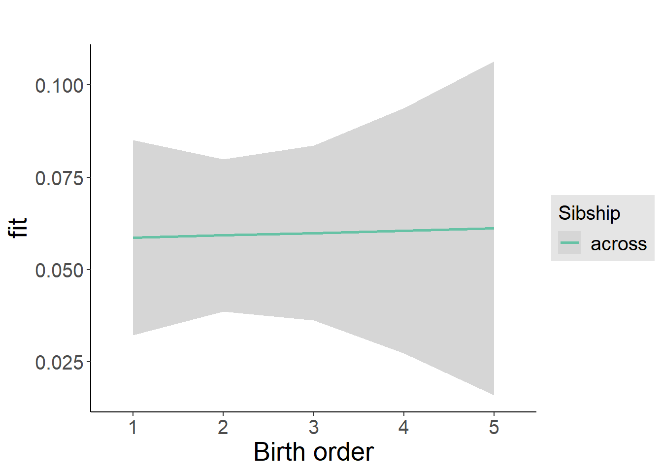
Add Birth Order Factor
Model Summary
m3_birthorder_nonlinear = update(m1_covariates_only, formula = . ~ . + birth_order_nonlinear)
tidy(m3_birthorder_nonlinear, conf.int = T, conf.level = 0.995)| effect | group | term | estimate | std.error | statistic | df | p.value | conf.low | conf.high |
|---|---|---|---|---|---|---|---|---|---|
| fixed | NA | (Intercept) | 0.6346 | 0.2151 | 2.951 | 2745 | 0.003199 | 0.03087 | 1.238 |
| fixed | NA | poly(age, 3, raw = TRUE)1 | -0.05422 | 0.02382 | -2.276 | 2745 | 0.02291 | -0.1211 | 0.01265 |
| fixed | NA | poly(age, 3, raw = TRUE)2 | 0.001602 | 0.0008447 | 1.897 | 2744 | 0.05797 | -0.0007689 | 0.003973 |
| fixed | NA | poly(age, 3, raw = TRUE)3 | -0.00001576 | 0.000009592 | -1.643 | 2742 | 0.1006 | -0.00004268 | 0.00001117 |
| fixed | NA | male | 0.05021 | 0.01008 | 4.98 | 2745 | 0.0000006752 | 0.02191 | 0.07851 |
| fixed | NA | sibling_count3 | -0.004761 | 0.01447 | -0.3291 | 2226 | 0.7421 | -0.04537 | 0.03585 |
| fixed | NA | sibling_count4 | 0.008754 | 0.01565 | 0.5593 | 2134 | 0.576 | -0.03518 | 0.05269 |
| fixed | NA | sibling_count5 | -0.01629 | 0.01861 | -0.8756 | 2049 | 0.3813 | -0.06852 | 0.03594 |
| fixed | NA | birth_order_nonlinear2 | 0.01022 | 0.01214 | 0.842 | 2330 | 0.3999 | -0.02386 | 0.0443 |
| fixed | NA | birth_order_nonlinear3 | -0.003476 | 0.01482 | -0.2345 | 2415 | 0.8146 | -0.04507 | 0.03812 |
| fixed | NA | birth_order_nonlinear4 | 0.003818 | 0.01967 | 0.1941 | 2499 | 0.8461 | -0.05141 | 0.05904 |
| fixed | NA | birth_order_nonlinear5 | 0.005898 | 0.03023 | 0.1951 | 2442 | 0.8453 | -0.07896 | 0.09076 |
| ran_pars | mother_pidlink | sd__(Intercept) | 0.07342 | NA | NA | NA | NA | NA | NA |
| ran_pars | Residual | sd__Observation | 0.251 | NA | NA | NA | NA | NA | NA |
Coefficient Plot
plot_birthorder(m3_birthorder_nonlinear, separate = FALSE)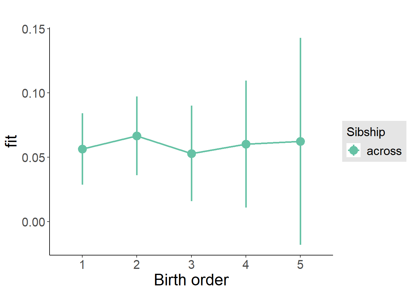
Add Interaction
Model Summary
m4_interaction = update(m3_birthorder_nonlinear, formula = . ~ . - birth_order_nonlinear - sibling_count + count_birth_order)
tidy(m4_interaction, conf.int = T, conf.level = 0.995)| effect | group | term | estimate | std.error | statistic | df | p.value | conf.low | conf.high |
|---|---|---|---|---|---|---|---|---|---|
| fixed | NA | (Intercept) | 0.6485 | 0.2153 | 3.013 | 2739 | 0.002614 | 0.04426 | 1.253 |
| fixed | NA | poly(age, 3, raw = TRUE)1 | -0.05463 | 0.02384 | -2.292 | 2739 | 0.022 | -0.1215 | 0.01229 |
| fixed | NA | poly(age, 3, raw = TRUE)2 | 0.001617 | 0.0008454 | 1.912 | 2738 | 0.05593 | -0.0007563 | 0.00399 |
| fixed | NA | poly(age, 3, raw = TRUE)3 | -0.00001592 | 0.000009602 | -1.658 | 2737 | 0.09749 | -0.00004287 | 0.00001104 |
| fixed | NA | male | 0.05061 | 0.0101 | 5.012 | 2739 | 0.0000005732 | 0.02226 | 0.07895 |
| fixed | NA | count_birth_order2/2 | -0.02243 | 0.02203 | -1.018 | 2367 | 0.3086 | -0.08428 | 0.03941 |
| fixed | NA | count_birth_order1/3 | -0.0172 | 0.01854 | -0.9279 | 2748 | 0.3535 | -0.06925 | 0.03484 |
| fixed | NA | count_birth_order2/3 | 0.002536 | 0.0206 | 0.1231 | 2750 | 0.902 | -0.05528 | 0.06036 |
| fixed | NA | count_birth_order3/3 | -0.02527 | 0.02229 | -1.133 | 2747 | 0.2572 | -0.08785 | 0.03731 |
| fixed | NA | count_birth_order1/4 | -0.01996 | 0.02137 | -0.9343 | 2749 | 0.3502 | -0.07994 | 0.04001 |
| fixed | NA | count_birth_order2/4 | 0.01785 | 0.02245 | 0.7951 | 2749 | 0.4267 | -0.04517 | 0.08086 |
| fixed | NA | count_birth_order3/4 | 0.003941 | 0.02355 | 0.1674 | 2744 | 0.8671 | -0.06215 | 0.07004 |
| fixed | NA | count_birth_order4/4 | 0.007373 | 0.02495 | 0.2955 | 2744 | 0.7676 | -0.06266 | 0.07741 |
| fixed | NA | count_birth_order1/5 | -0.02195 | 0.0281 | -0.7809 | 2750 | 0.4349 | -0.1008 | 0.05694 |
| fixed | NA | count_birth_order2/5 | -0.01095 | 0.03054 | -0.3585 | 2741 | 0.72 | -0.09667 | 0.07477 |
| fixed | NA | count_birth_order3/5 | -0.03344 | 0.02858 | -1.17 | 2741 | 0.2421 | -0.1137 | 0.04678 |
| fixed | NA | count_birth_order4/5 | -0.03001 | 0.02777 | -1.081 | 2738 | 0.2799 | -0.108 | 0.04794 |
| fixed | NA | count_birth_order5/5 | -0.02109 | 0.02912 | -0.7242 | 2734 | 0.469 | -0.1028 | 0.06064 |
| ran_pars | mother_pidlink | sd__(Intercept) | 0.07333 | NA | NA | NA | NA | NA | NA |
| ran_pars | Residual | sd__Observation | 0.2511 | NA | NA | NA | NA | NA | NA |
Coefficient Plot
plot_birthorder(m4_interaction)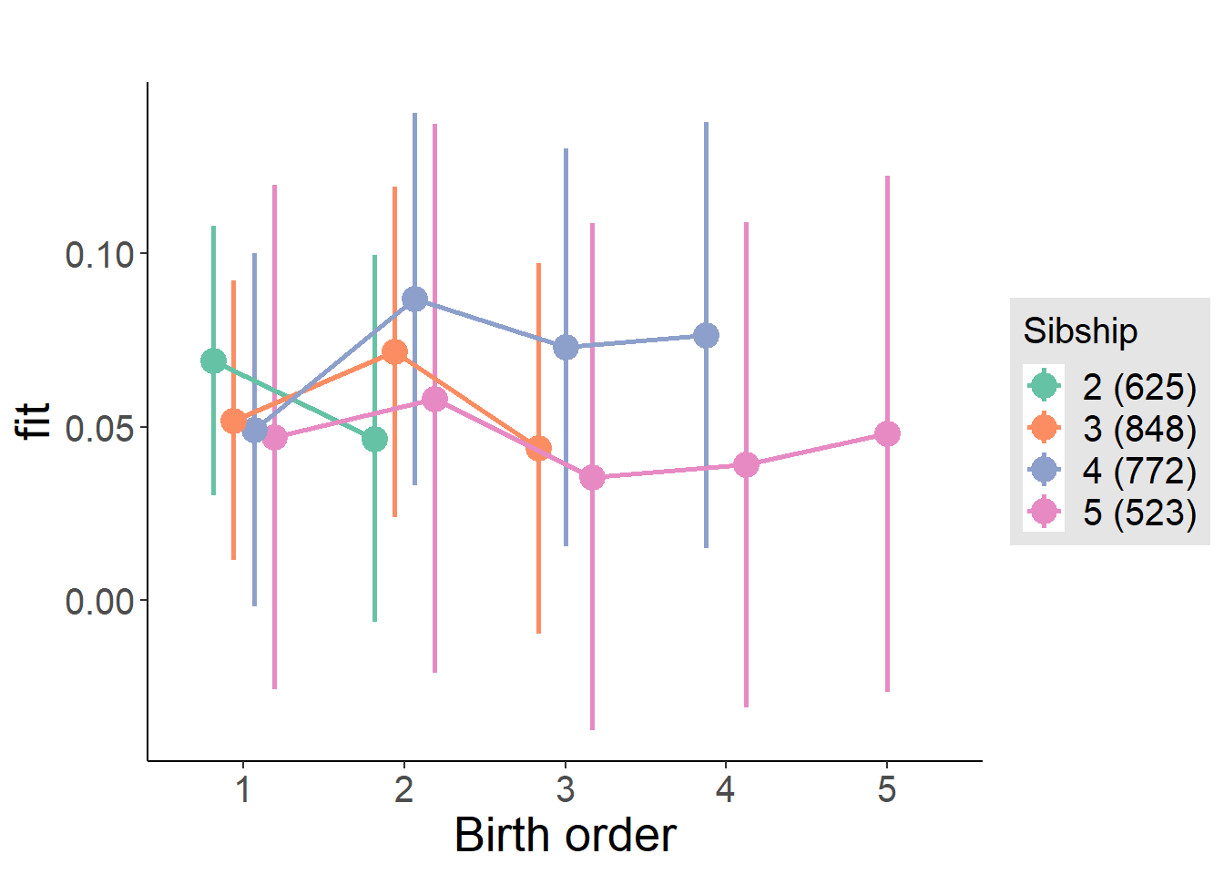
Model Comparison
###### Model 1 - Model 2
anova(m1_covariates_only, m2_birthorder_linear, m3_birthorder_nonlinear, m4_interaction)## refitting model(s) with ML (instead of REML)| Df | AIC | BIC | logLik | deviance | Chisq | Chi Df | Pr(>Chisq) |
|---|---|---|---|---|---|---|---|
| 10 | 434.2 | 493.4 | -207.1 | 414.2 | NA | NA | NA |
| 11 | 436.2 | 501.4 | -207.1 | 414.2 | 0.01566 | 1 | 0.9004 |
| 14 | 441.1 | 524.1 | -206.6 | 413.1 | 1.053 | 3 | 0.7884 |
| 20 | 448.6 | 567.1 | -204.3 | 408.6 | 4.535 | 6 | 0.6047 |
Maternal pregnancy order
outcome_preg_m1 <- update(m2_birthorder_linear, data = birthorder %>%
mutate(sibling_count = sibling_count_uterus_preg_factor,
birth_order_nonlinear = birthorder_uterus_preg_factor,
birth_order = birthorder_uterus_preg,
count_birth_order = count_birthorder_uterus_preg
) %>%
filter(sibling_count != "1"))
compare_models_markdown(outcome_preg_m1)Basic Model
Model Summary
m1_covariates_only <- update(m2_birthorder_linear, formula = . ~ . - birth_order)
tidy(m1_covariates_only, conf.int = T, conf.level = 0.995)| effect | group | term | estimate | std.error | statistic | df | p.value | conf.low | conf.high |
|---|---|---|---|---|---|---|---|---|---|
| fixed | NA | (Intercept) | 0.5885 | 0.2234 | 2.635 | 2526 | 0.008467 | -0.03845 | 1.215 |
| fixed | NA | poly(age, 3, raw = TRUE)1 | -0.04894 | 0.02476 | -1.977 | 2526 | 0.0482 | -0.1184 | 0.02056 |
| fixed | NA | poly(age, 3, raw = TRUE)2 | 0.001414 | 0.000878 | 1.611 | 2525 | 0.1074 | -0.00105 | 0.003879 |
| fixed | NA | poly(age, 3, raw = TRUE)3 | -0.00001364 | 0.000009972 | -1.368 | 2524 | 0.1715 | -0.00004163 | 0.00001435 |
| fixed | NA | male | 0.05694 | 0.01057 | 5.388 | 2517 | 0.00000007771 | 0.02728 | 0.08661 |
| fixed | NA | sibling_count3 | -0.01313 | 0.01549 | -0.8472 | 1997 | 0.397 | -0.05662 | 0.03036 |
| fixed | NA | sibling_count4 | -0.005705 | 0.01568 | -0.3639 | 1886 | 0.7159 | -0.04971 | 0.0383 |
| fixed | NA | sibling_count5 | 0.008204 | 0.01653 | 0.4963 | 1711 | 0.6197 | -0.0382 | 0.0546 |
| ran_pars | mother_pidlink | sd__(Intercept) | 0.07984 | NA | NA | NA | NA | NA | NA |
| ran_pars | Residual | sd__Observation | 0.2503 | NA | NA | NA | NA | NA | NA |
Coefficient Plot
plot(allEffects(m1_covariates_only, confidence.level = 0.995))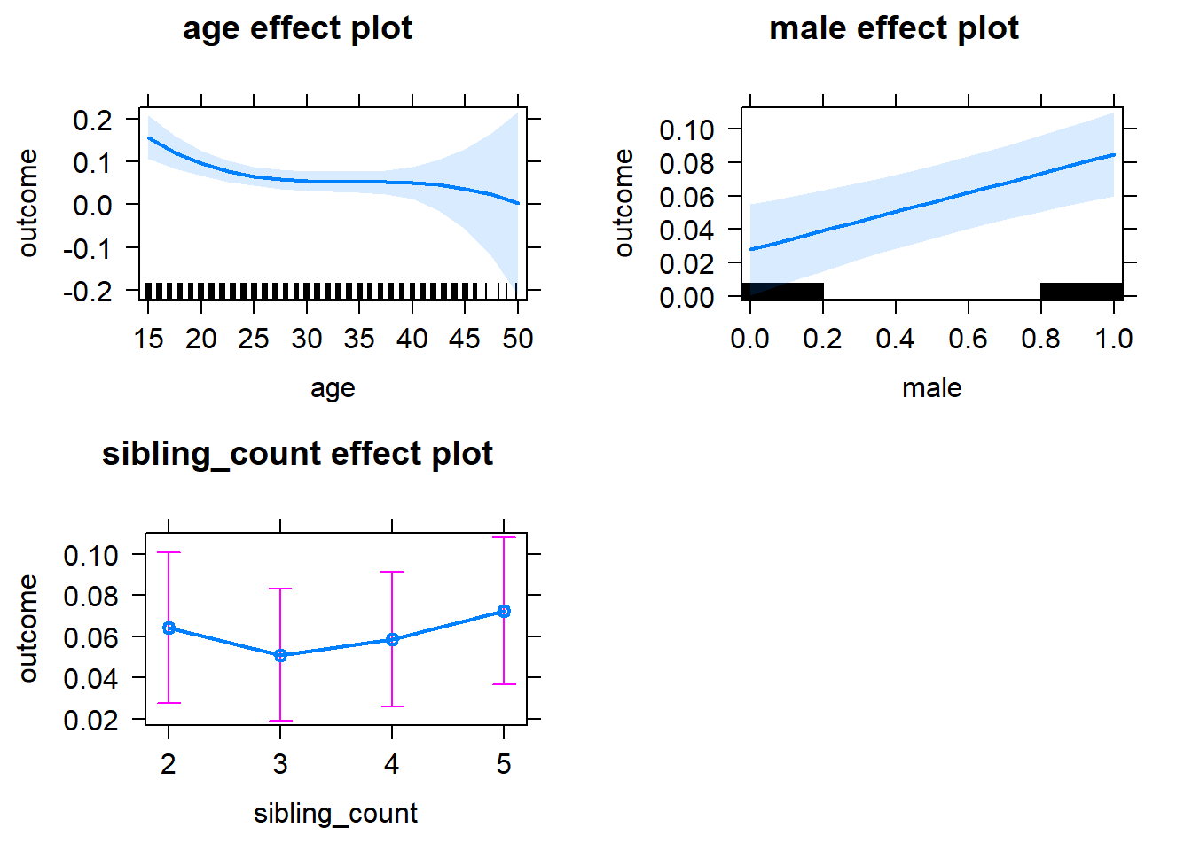
Add Birth Order Linear
Model Summary
tidy(m2_birthorder_linear, conf.int = T, conf.level = 0.995)| effect | group | term | estimate | std.error | statistic | df | p.value | conf.low | conf.high |
|---|---|---|---|---|---|---|---|---|---|
| fixed | NA | (Intercept) | 0.5916 | 0.2234 | 2.648 | 2525 | 0.008156 | -0.03562 | 1.219 |
| fixed | NA | birth_order | -0.002964 | 0.005159 | -0.5745 | 2436 | 0.5657 | -0.01745 | 0.01152 |
| fixed | NA | poly(age, 3, raw = TRUE)1 | -0.04889 | 0.02476 | -1.974 | 2525 | 0.04846 | -0.1184 | 0.02062 |
| fixed | NA | poly(age, 3, raw = TRUE)2 | 0.001416 | 0.0008781 | 1.613 | 2524 | 0.1069 | -0.001049 | 0.003881 |
| fixed | NA | poly(age, 3, raw = TRUE)3 | -0.00001373 | 0.000009975 | -1.376 | 2523 | 0.1689 | -0.00004173 | 0.00001427 |
| fixed | NA | male | 0.05685 | 0.01057 | 5.378 | 2516 | 0.00000008231 | 0.02718 | 0.08652 |
| fixed | NA | sibling_count3 | -0.01166 | 0.0157 | -0.7424 | 2018 | 0.4579 | -0.05574 | 0.03242 |
| fixed | NA | sibling_count4 | -0.002849 | 0.01645 | -0.1732 | 1970 | 0.8625 | -0.04902 | 0.04332 |
| fixed | NA | sibling_count5 | 0.01299 | 0.01851 | 0.7017 | 1954 | 0.4829 | -0.03897 | 0.06495 |
| ran_pars | mother_pidlink | sd__(Intercept) | 0.07984 | NA | NA | NA | NA | NA | NA |
| ran_pars | Residual | sd__Observation | 0.2503 | NA | NA | NA | NA | NA | NA |
Coefficient Plot
plot_birthorder2(m2_birthorder_linear, separate = FALSE)
Add Birth Order Factor
Model Summary
m3_birthorder_nonlinear = update(m1_covariates_only, formula = . ~ . + birth_order_nonlinear)
tidy(m3_birthorder_nonlinear, conf.int = T, conf.level = 0.995)| effect | group | term | estimate | std.error | statistic | df | p.value | conf.low | conf.high |
|---|---|---|---|---|---|---|---|---|---|
| fixed | NA | (Intercept) | 0.5829 | 0.224 | 2.603 | 2520 | 0.009306 | -0.04578 | 1.212 |
| fixed | NA | poly(age, 3, raw = TRUE)1 | -0.04867 | 0.02482 | -1.961 | 2520 | 0.04999 | -0.1183 | 0.021 |
| fixed | NA | poly(age, 3, raw = TRUE)2 | 0.001406 | 0.0008802 | 1.597 | 2520 | 0.1104 | -0.001065 | 0.003876 |
| fixed | NA | poly(age, 3, raw = TRUE)3 | -0.00001359 | 0.000009997 | -1.359 | 2519 | 0.1742 | -0.00004165 | 0.00001447 |
| fixed | NA | male | 0.05688 | 0.01058 | 5.377 | 2513 | 0.00000008265 | 0.02718 | 0.08657 |
| fixed | NA | sibling_count3 | -0.0115 | 0.01594 | -0.7215 | 2069 | 0.4707 | -0.05624 | 0.03324 |
| fixed | NA | sibling_count4 | -0.002333 | 0.01666 | -0.1401 | 2018 | 0.8886 | -0.04909 | 0.04443 |
| fixed | NA | sibling_count5 | 0.01508 | 0.01863 | 0.8094 | 1976 | 0.4184 | -0.03722 | 0.06739 |
| fixed | NA | birth_order_nonlinear2 | 0.01122 | 0.01265 | 0.8872 | 2145 | 0.3751 | -0.02428 | 0.04672 |
| fixed | NA | birth_order_nonlinear3 | -0.005925 | 0.01559 | -0.3801 | 2258 | 0.7039 | -0.04968 | 0.03783 |
| fixed | NA | birth_order_nonlinear4 | -0.007512 | 0.02043 | -0.3678 | 2323 | 0.7131 | -0.06485 | 0.04983 |
| fixed | NA | birth_order_nonlinear5 | -0.01462 | 0.02921 | -0.5003 | 2253 | 0.6169 | -0.09662 | 0.06739 |
| ran_pars | mother_pidlink | sd__(Intercept) | 0.08006 | NA | NA | NA | NA | NA | NA |
| ran_pars | Residual | sd__Observation | 0.2503 | NA | NA | NA | NA | NA | NA |
Coefficient Plot
plot_birthorder(m3_birthorder_nonlinear, separate = FALSE)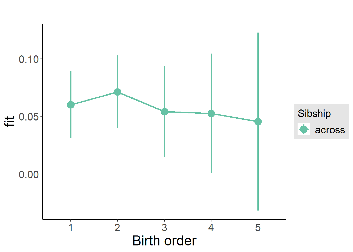
Add Interaction
Model Summary
m4_interaction = update(m3_birthorder_nonlinear, formula = . ~ . - birth_order_nonlinear - sibling_count + count_birth_order)
tidy(m4_interaction, conf.int = T, conf.level = 0.995)| effect | group | term | estimate | std.error | statistic | df | p.value | conf.low | conf.high |
|---|---|---|---|---|---|---|---|---|---|
| fixed | NA | (Intercept) | 0.5927 | 0.2243 | 2.643 | 2514 | 0.008276 | -0.03686 | 1.222 |
| fixed | NA | poly(age, 3, raw = TRUE)1 | -0.04877 | 0.02485 | -1.963 | 2514 | 0.0498 | -0.1185 | 0.02098 |
| fixed | NA | poly(age, 3, raw = TRUE)2 | 0.001409 | 0.0008813 | 1.598 | 2513 | 0.1101 | -0.001065 | 0.003882 |
| fixed | NA | poly(age, 3, raw = TRUE)3 | -0.0000136 | 0.00001001 | -1.359 | 2512 | 0.1743 | -0.0000417 | 0.0000145 |
| fixed | NA | male | 0.05703 | 0.01061 | 5.377 | 2508 | 0.00000008251 | 0.02726 | 0.0868 |
| fixed | NA | count_birth_order2/2 | -0.01636 | 0.02431 | -0.6728 | 2233 | 0.5012 | -0.08459 | 0.05188 |
| fixed | NA | count_birth_order1/3 | -0.02062 | 0.0206 | -1.001 | 2519 | 0.317 | -0.07844 | 0.03721 |
| fixed | NA | count_birth_order2/3 | -0.002162 | 0.0224 | -0.09651 | 2521 | 0.9231 | -0.06504 | 0.06072 |
| fixed | NA | count_birth_order3/3 | -0.03625 | 0.02464 | -1.471 | 2518 | 0.1414 | -0.1054 | 0.03292 |
| fixed | NA | count_birth_order1/4 | -0.0266 | 0.02247 | -1.184 | 2520 | 0.2367 | -0.08968 | 0.03648 |
| fixed | NA | count_birth_order2/4 | 0.007569 | 0.02343 | 0.323 | 2521 | 0.7467 | -0.05821 | 0.07335 |
| fixed | NA | count_birth_order3/4 | -0.01562 | 0.02561 | -0.6097 | 2515 | 0.5421 | -0.08751 | 0.05628 |
| fixed | NA | count_birth_order4/4 | -0.005454 | 0.02731 | -0.1997 | 2513 | 0.8417 | -0.08211 | 0.0712 |
| fixed | NA | count_birth_order1/5 | 0.008708 | 0.02699 | 0.3226 | 2521 | 0.747 | -0.06706 | 0.08447 |
| fixed | NA | count_birth_order2/5 | 0.01577 | 0.02801 | 0.5628 | 2518 | 0.5736 | -0.06286 | 0.0944 |
| fixed | NA | count_birth_order3/5 | 0.01232 | 0.02849 | 0.4324 | 2512 | 0.6655 | -0.06765 | 0.09228 |
| fixed | NA | count_birth_order4/5 | -0.01694 | 0.02891 | -0.5858 | 2506 | 0.558 | -0.0981 | 0.06422 |
| fixed | NA | count_birth_order5/5 | -0.008884 | 0.02913 | -0.305 | 2503 | 0.7604 | -0.09065 | 0.07288 |
| ran_pars | mother_pidlink | sd__(Intercept) | 0.07844 | NA | NA | NA | NA | NA | NA |
| ran_pars | Residual | sd__Observation | 0.2509 | NA | NA | NA | NA | NA | NA |
Coefficient Plot
plot_birthorder(m4_interaction)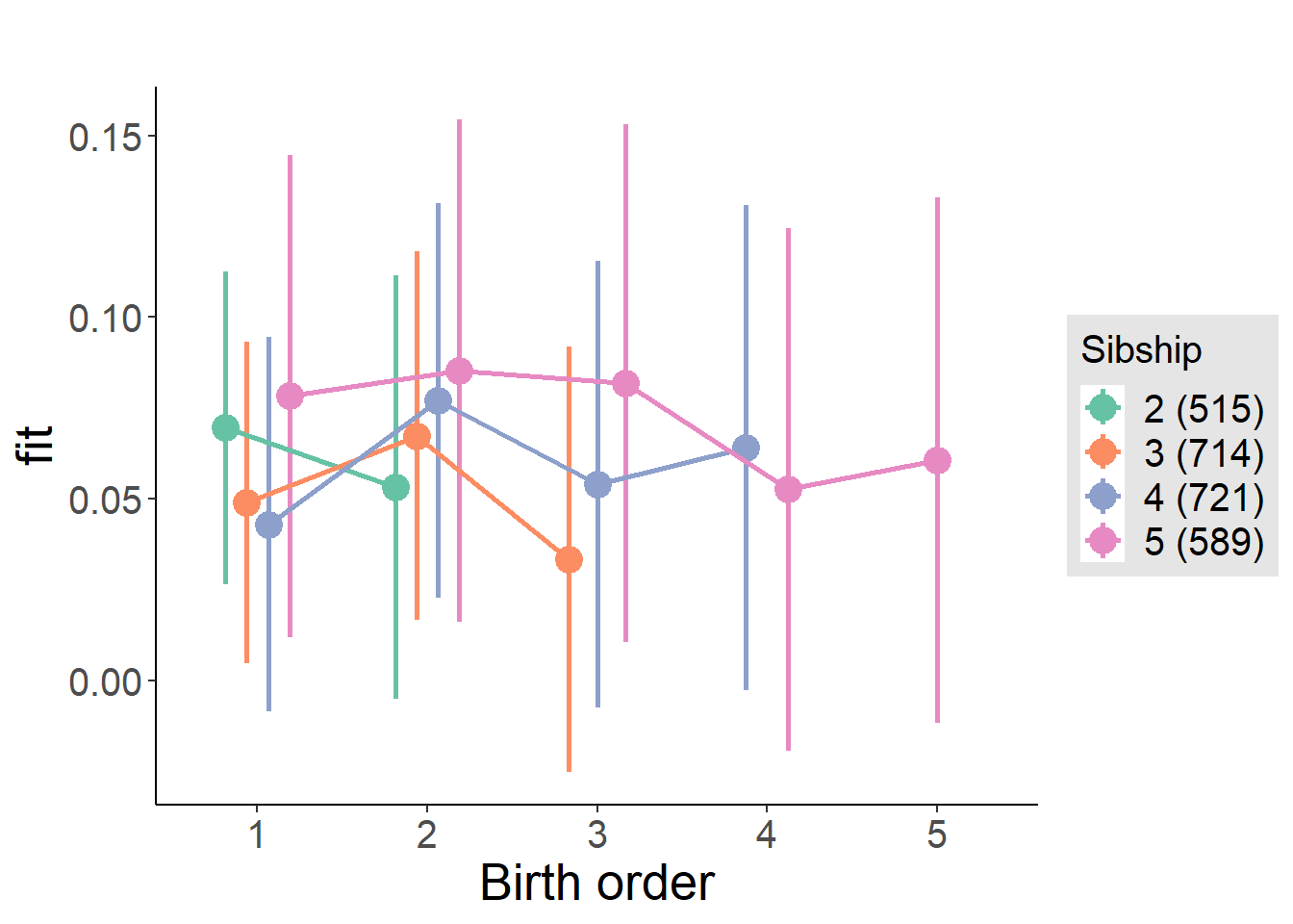
Model Comparison
###### Model 1 - Model 2
anova(m1_covariates_only, m2_birthorder_linear, m3_birthorder_nonlinear, m4_interaction)## refitting model(s) with ML (instead of REML)| Df | AIC | BIC | logLik | deviance | Chisq | Chi Df | Pr(>Chisq) |
|---|---|---|---|---|---|---|---|
| 10 | 422.4 | 480.8 | -201.2 | 402.4 | NA | NA | NA |
| 11 | 424.1 | 488.3 | -201 | 402.1 | 0.331 | 1 | 0.5651 |
| 14 | 428.5 | 510.3 | -200.3 | 400.5 | 1.551 | 3 | 0.6706 |
| 20 | 436.8 | 553.6 | -198.4 | 396.8 | 3.72 | 6 | 0.7145 |
Parental full sibling order
outcome_parental_m1 <- update(m2_birthorder_linear, data = birthorder %>%
mutate(sibling_count = sibling_count_genes_factor,
birth_order_nonlinear = birthorder_genes_factor,
birth_order = birthorder_genes,
count_birth_order = count_birthorder_genes
) %>%
filter(sibling_count != "1"))
compare_models_markdown(outcome_parental_m1)Basic Model
Model Summary
m1_covariates_only <- update(m2_birthorder_linear, formula = . ~ . - birth_order)
tidy(m1_covariates_only, conf.int = T, conf.level = 0.995)| effect | group | term | estimate | std.error | statistic | df | p.value | conf.low | conf.high |
|---|---|---|---|---|---|---|---|---|---|
| fixed | NA | (Intercept) | 0.6357 | 0.2163 | 2.939 | 2746 | 0.003324 | 0.02847 | 1.243 |
| fixed | NA | poly(age, 3, raw = TRUE)1 | -0.0548 | 0.02403 | -2.281 | 2746 | 0.02264 | -0.1223 | 0.01265 |
| fixed | NA | poly(age, 3, raw = TRUE)2 | 0.001642 | 0.000854 | 1.922 | 2744 | 0.0547 | -0.0007558 | 0.004039 |
| fixed | NA | poly(age, 3, raw = TRUE)3 | -0.00001622 | 0.000009725 | -1.668 | 2742 | 0.09545 | -0.00004352 | 0.00001108 |
| fixed | NA | male | 0.05342 | 0.01006 | 5.312 | 2750 | 0.0000001171 | 0.02519 | 0.08165 |
| fixed | NA | sibling_count3 | -0.008121 | 0.01371 | -0.5924 | 2144 | 0.5537 | -0.0466 | 0.03036 |
| fixed | NA | sibling_count4 | 0.001207 | 0.01439 | 0.08388 | 1946 | 0.9332 | -0.03919 | 0.0416 |
| fixed | NA | sibling_count5 | -0.02306 | 0.0164 | -1.406 | 1591 | 0.1599 | -0.0691 | 0.02298 |
| ran_pars | mother_pidlink | sd__(Intercept) | 0.07058 | NA | NA | NA | NA | NA | NA |
| ran_pars | Residual | sd__Observation | 0.2512 | NA | NA | NA | NA | NA | NA |
Coefficient Plot
plot(allEffects(m1_covariates_only, confidence.level = 0.995))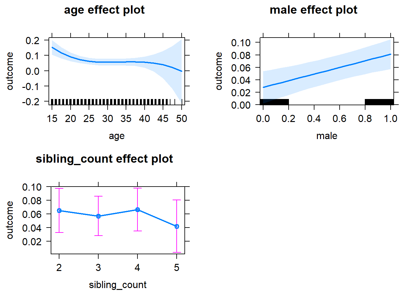
Add Birth Order Linear
Model Summary
tidy(m2_birthorder_linear, conf.int = T, conf.level = 0.995)| effect | group | term | estimate | std.error | statistic | df | p.value | conf.low | conf.high |
|---|---|---|---|---|---|---|---|---|---|
| fixed | NA | (Intercept) | 0.6355 | 0.2164 | 2.936 | 2746 | 0.003347 | 0.02801 | 1.243 |
| fixed | NA | birth_order | 0.0005298 | 0.005132 | 0.1032 | 2602 | 0.9178 | -0.01388 | 0.01494 |
| fixed | NA | poly(age, 3, raw = TRUE)1 | -0.05484 | 0.02403 | -2.282 | 2744 | 0.02259 | -0.1223 | 0.01263 |
| fixed | NA | poly(age, 3, raw = TRUE)2 | 0.001642 | 0.0008542 | 1.922 | 2743 | 0.05471 | -0.000756 | 0.00404 |
| fixed | NA | poly(age, 3, raw = TRUE)3 | -0.00001621 | 0.000009727 | -1.666 | 2741 | 0.09573 | -0.00004351 | 0.00001109 |
| fixed | NA | male | 0.05342 | 0.01006 | 5.312 | 2749 | 0.0000001174 | 0.02519 | 0.08166 |
| fixed | NA | sibling_count3 | -0.008379 | 0.01394 | -0.6012 | 2176 | 0.5478 | -0.0475 | 0.03074 |
| fixed | NA | sibling_count4 | 0.000669 | 0.0153 | 0.04371 | 2089 | 0.9651 | -0.04229 | 0.04363 |
| fixed | NA | sibling_count5 | -0.02394 | 0.0185 | -1.294 | 1913 | 0.1957 | -0.07586 | 0.02798 |
| ran_pars | mother_pidlink | sd__(Intercept) | 0.07055 | NA | NA | NA | NA | NA | NA |
| ran_pars | Residual | sd__Observation | 0.2513 | NA | NA | NA | NA | NA | NA |
Coefficient Plot
plot_birthorder2(m2_birthorder_linear, separate = FALSE)
Add Birth Order Factor
Model Summary
m3_birthorder_nonlinear = update(m1_covariates_only, formula = . ~ . + birth_order_nonlinear)
tidy(m3_birthorder_nonlinear, conf.int = T, conf.level = 0.995)| effect | group | term | estimate | std.error | statistic | df | p.value | conf.low | conf.high |
|---|---|---|---|---|---|---|---|---|---|
| fixed | NA | (Intercept) | 0.6307 | 0.2168 | 2.909 | 2741 | 0.003657 | 0.02208 | 1.239 |
| fixed | NA | poly(age, 3, raw = TRUE)1 | -0.05457 | 0.02408 | -2.267 | 2741 | 0.0235 | -0.1222 | 0.01301 |
| fixed | NA | poly(age, 3, raw = TRUE)2 | 0.001631 | 0.0008558 | 1.906 | 2739 | 0.05676 | -0.0007711 | 0.004033 |
| fixed | NA | poly(age, 3, raw = TRUE)3 | -0.00001609 | 0.000009744 | -1.651 | 2738 | 0.09882 | -0.00004344 | 0.00001126 |
| fixed | NA | male | 0.05339 | 0.01007 | 5.303 | 2747 | 0.0000001231 | 0.02513 | 0.08165 |
| fixed | NA | sibling_count3 | -0.008208 | 0.01417 | -0.5793 | 2244 | 0.5624 | -0.04798 | 0.03156 |
| fixed | NA | sibling_count4 | 0.002095 | 0.01552 | 0.135 | 2152 | 0.8926 | -0.04146 | 0.04565 |
| fixed | NA | sibling_count5 | -0.02175 | 0.01881 | -1.156 | 1969 | 0.2479 | -0.07456 | 0.03107 |
| fixed | NA | birth_order_nonlinear2 | 0.01148 | 0.01201 | 0.9556 | 2334 | 0.3394 | -0.02223 | 0.04518 |
| fixed | NA | birth_order_nonlinear3 | 0.001848 | 0.01477 | 0.1251 | 2425 | 0.9005 | -0.03962 | 0.04331 |
| fixed | NA | birth_order_nonlinear4 | -0.002733 | 0.0202 | -0.1353 | 2506 | 0.8924 | -0.05942 | 0.05396 |
| fixed | NA | birth_order_nonlinear5 | 0.004468 | 0.03185 | 0.1403 | 2465 | 0.8884 | -0.08493 | 0.09387 |
| ran_pars | mother_pidlink | sd__(Intercept) | 0.07032 | NA | NA | NA | NA | NA | NA |
| ran_pars | Residual | sd__Observation | 0.2514 | NA | NA | NA | NA | NA | NA |
Coefficient Plot
plot_birthorder(m3_birthorder_nonlinear, separate = FALSE)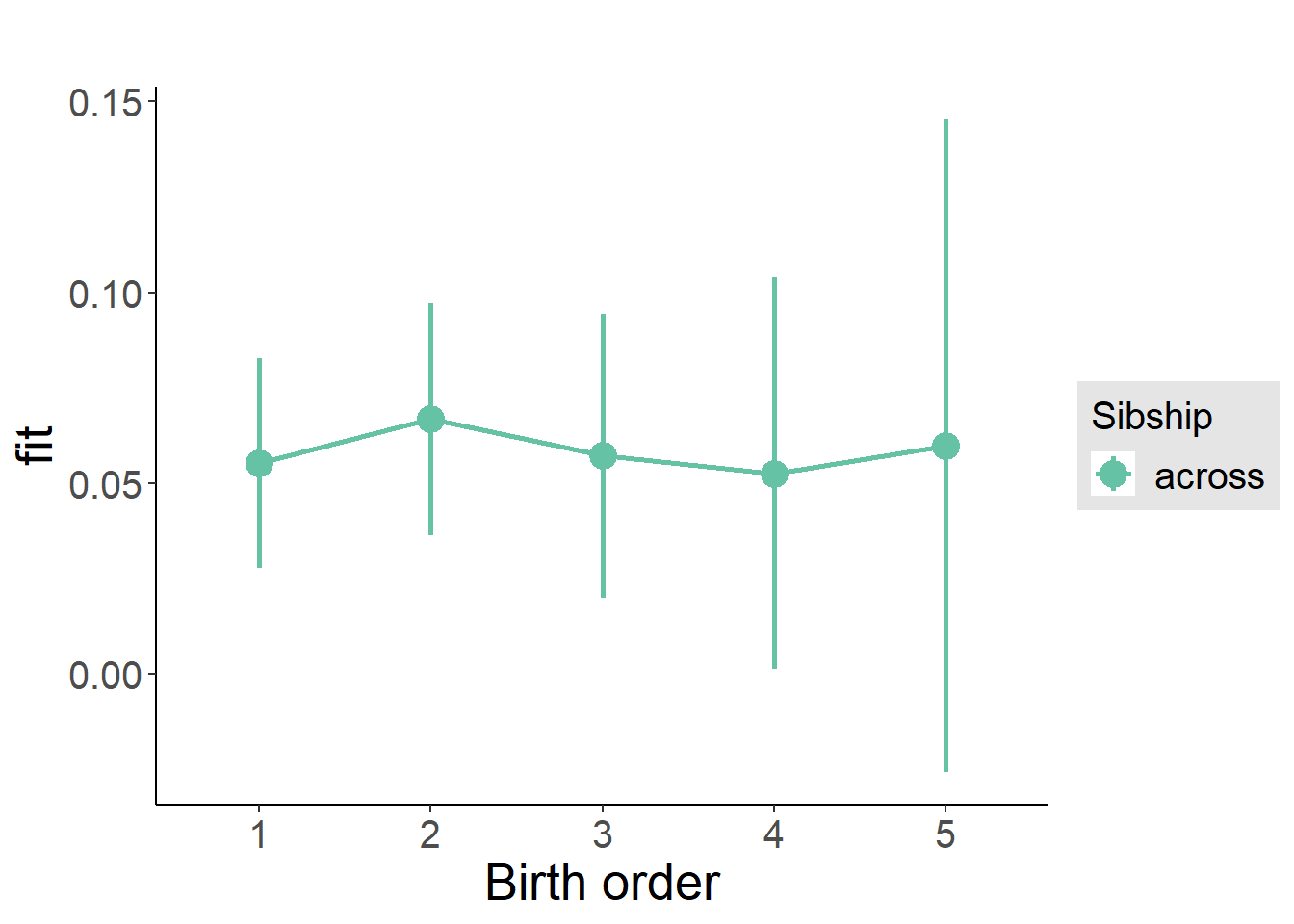
Add Interaction
Model Summary
m4_interaction = update(m3_birthorder_nonlinear, formula = . ~ . - birth_order_nonlinear - sibling_count + count_birth_order)
tidy(m4_interaction, conf.int = T, conf.level = 0.995)| effect | group | term | estimate | std.error | statistic | df | p.value | conf.low | conf.high |
|---|---|---|---|---|---|---|---|---|---|
| fixed | NA | (Intercept) | 0.6386 | 0.217 | 2.942 | 2736 | 0.003287 | 0.02932 | 1.248 |
| fixed | NA | poly(age, 3, raw = TRUE)1 | -0.05456 | 0.0241 | -2.264 | 2735 | 0.02367 | -0.1222 | 0.0131 |
| fixed | NA | poly(age, 3, raw = TRUE)2 | 0.001629 | 0.0008568 | 1.902 | 2734 | 0.05732 | -0.0007757 | 0.004034 |
| fixed | NA | poly(age, 3, raw = TRUE)3 | -0.00001606 | 0.000009757 | -1.646 | 2732 | 0.09997 | -0.00004344 | 0.00001133 |
| fixed | NA | male | 0.05378 | 0.01008 | 5.333 | 2741 | 0.0000001043 | 0.02547 | 0.08208 |
| fixed | NA | count_birth_order2/2 | -0.01225 | 0.0214 | -0.5723 | 2362 | 0.5672 | -0.07232 | 0.04783 |
| fixed | NA | count_birth_order1/3 | -0.01725 | 0.0182 | -0.9474 | 2748 | 0.3435 | -0.06834 | 0.03385 |
| fixed | NA | count_birth_order2/3 | 0.0003877 | 0.02025 | 0.01914 | 2750 | 0.9847 | -0.05646 | 0.05724 |
| fixed | NA | count_birth_order3/3 | -0.01829 | 0.0217 | -0.8428 | 2746 | 0.3994 | -0.07919 | 0.04262 |
| fixed | NA | count_birth_order1/4 | -0.0183 | 0.02141 | -0.8547 | 2750 | 0.3928 | -0.07841 | 0.04181 |
| fixed | NA | count_birth_order2/4 | 0.007508 | 0.02236 | 0.3358 | 2748 | 0.7371 | -0.05526 | 0.07027 |
| fixed | NA | count_birth_order3/4 | 0.005346 | 0.02344 | 0.2281 | 2744 | 0.8196 | -0.06045 | 0.07114 |
| fixed | NA | count_birth_order4/4 | -0.001617 | 0.02525 | -0.06401 | 2745 | 0.949 | -0.07251 | 0.06927 |
| fixed | NA | count_birth_order1/5 | -0.03018 | 0.02808 | -1.074 | 2750 | 0.2827 | -0.109 | 0.04866 |
| fixed | NA | count_birth_order2/5 | 0.002559 | 0.03149 | 0.08127 | 2741 | 0.9352 | -0.08582 | 0.09094 |
| fixed | NA | count_birth_order3/5 | -0.03558 | 0.03011 | -1.182 | 2740 | 0.2375 | -0.1201 | 0.04895 |
| fixed | NA | count_birth_order4/5 | -0.04183 | 0.02901 | -1.442 | 2739 | 0.1494 | -0.1233 | 0.0396 |
| fixed | NA | count_birth_order5/5 | -0.02515 | 0.03054 | -0.8237 | 2736 | 0.4102 | -0.1109 | 0.06056 |
| ran_pars | mother_pidlink | sd__(Intercept) | 0.07033 | NA | NA | NA | NA | NA | NA |
| ran_pars | Residual | sd__Observation | 0.2516 | NA | NA | NA | NA | NA | NA |
Coefficient Plot
plot_birthorder(m4_interaction)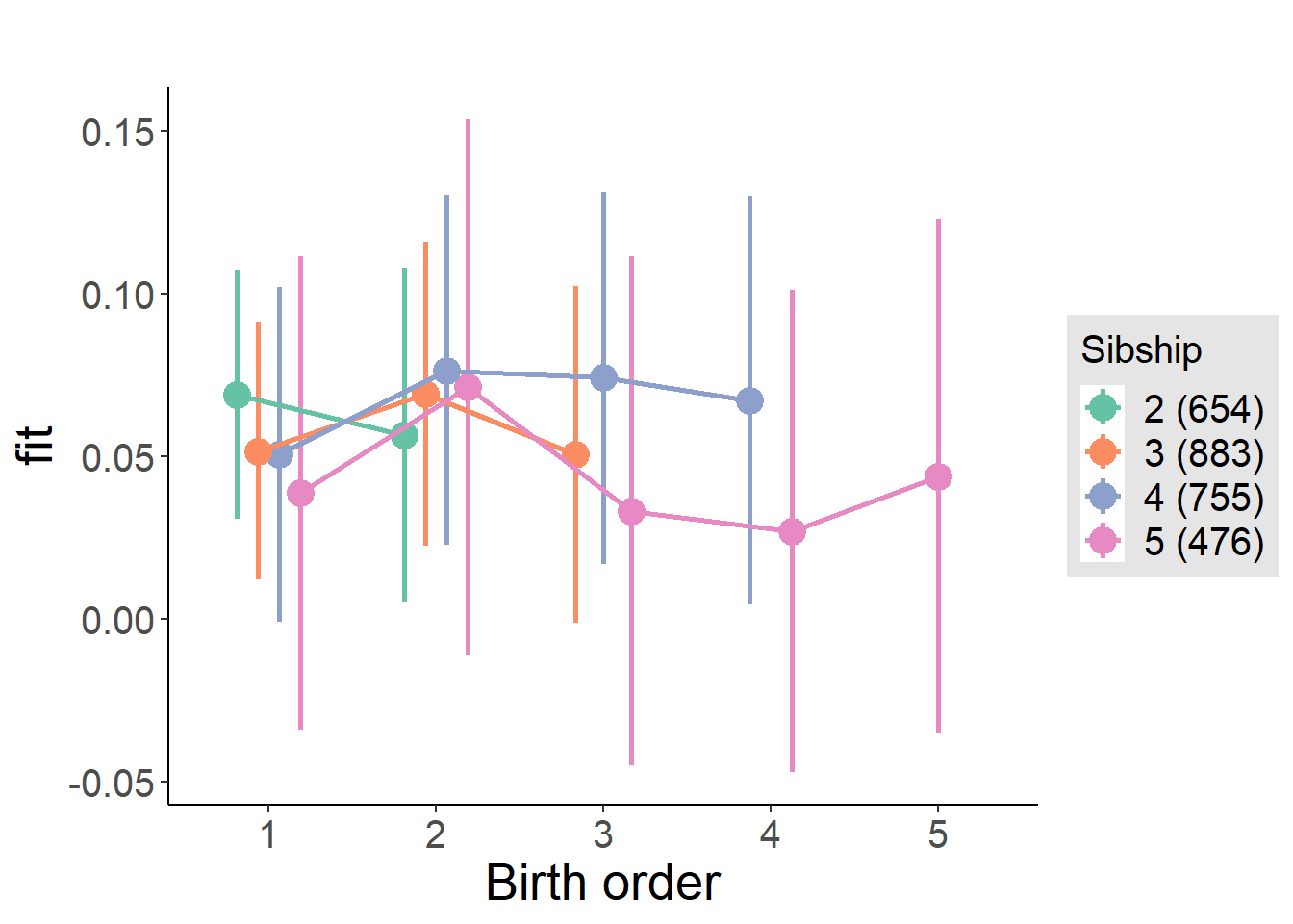
Model Comparison
###### Model 1 - Model 2
anova(m1_covariates_only, m2_birthorder_linear, m3_birthorder_nonlinear, m4_interaction)## refitting model(s) with ML (instead of REML)| Df | AIC | BIC | logLik | deviance | Chisq | Chi Df | Pr(>Chisq) |
|---|---|---|---|---|---|---|---|
| 10 | 424.8 | 484.1 | -202.4 | 404.8 | NA | NA | NA |
| 11 | 426.8 | 492 | -202.4 | 404.8 | 0.01064 | 1 | 0.9178 |
| 14 | 431.7 | 514.7 | -201.9 | 403.7 | 1.1 | 3 | 0.777 |
| 20 | 440.7 | 559.2 | -200.3 | 400.7 | 3.055 | 6 | 0.8019 |
Compare birth order specifications
library(coefplot)
multiplot(outcome_naive_m1, outcome_preg_m1, outcome_uterus_m1, outcome_parental_m1, dodgeHeight = 0.6,
intercept = FALSE)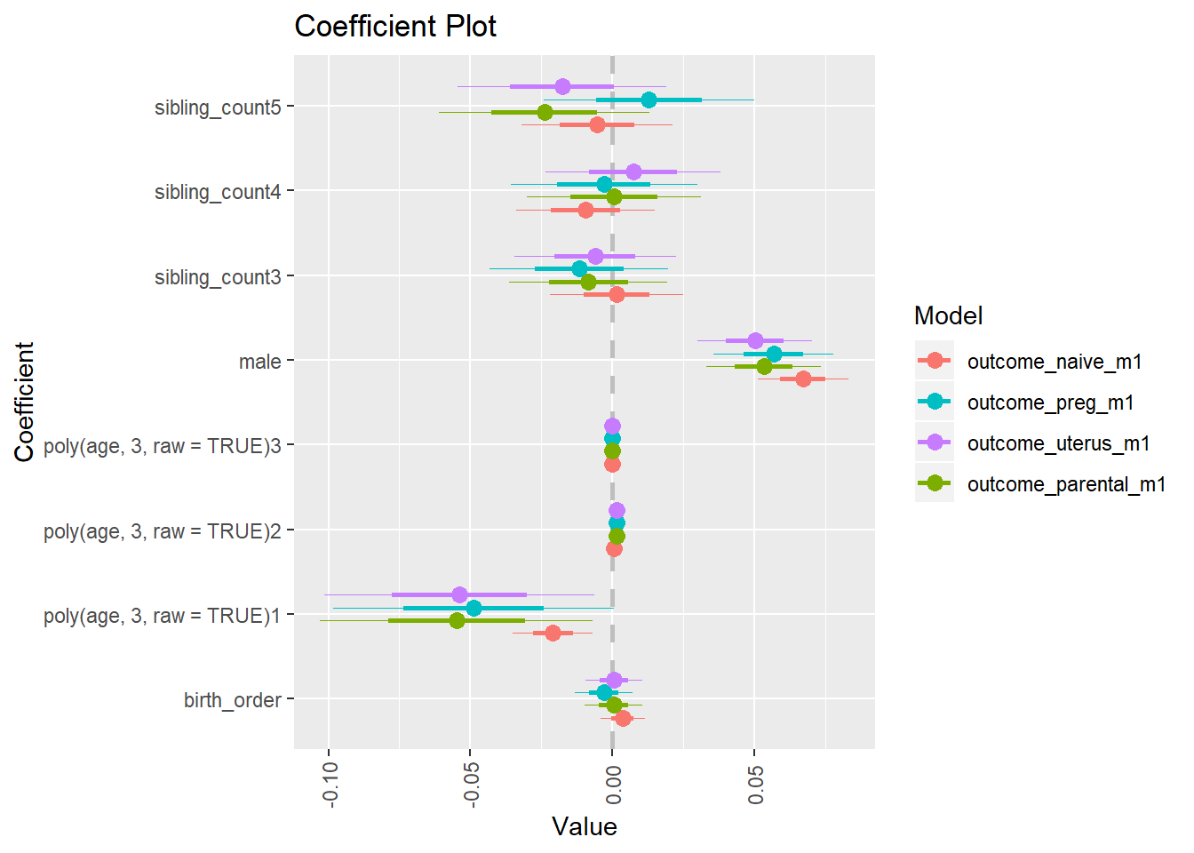
Category_Government worker
birthorder <- birthorder %>% mutate(outcome = `Category_Government worker`)
model = lmer(outcome ~ birth_order + poly(age, 3, raw = TRUE) + male + sibling_count + (1 | mother_pidlink),
data = birthorder)
compare_birthorder_specs(model)Naive birth order
outcome_naive_m1 <- update(m2_birthorder_linear, data = birthorder %>%
mutate(sibling_count = sibling_count_naive_factor,
birth_order_nonlinear = birthorder_naive_factor,
birth_order = birthorder_naive,
count_birth_order = count_birthorder_naive) %>%
filter(sibling_count != "1"))
compare_models_markdown(outcome_naive_m1)Basic Model
Model Summary
m1_covariates_only <- update(m2_birthorder_linear, formula = . ~ . - birth_order)
tidy(m1_covariates_only, conf.int = T, conf.level = 0.995)| effect | group | term | estimate | std.error | statistic | df | p.value | conf.low | conf.high |
|---|---|---|---|---|---|---|---|---|---|
| fixed | NA | (Intercept) | -0.2372 | 0.07472 | -3.174 | 4592 | 0.001513 | -0.4469 | -0.02742 |
| fixed | NA | poly(age, 3, raw = TRUE)1 | 0.02161 | 0.006676 | 3.237 | 4525 | 0.001218 | 0.002868 | 0.04035 |
| fixed | NA | poly(age, 3, raw = TRUE)2 | -0.000444 | 0.0001858 | -2.39 | 4435 | 0.01689 | -0.0009654 | 0.00007746 |
| fixed | NA | poly(age, 3, raw = TRUE)3 | 0.000002937 | 0.000001627 | 1.805 | 4349 | 0.07115 | -0.00000163 | 0.000007504 |
| fixed | NA | male | -0.02212 | 0.007447 | -2.97 | 4679 | 0.002994 | -0.04302 | -0.001213 |
| fixed | NA | sibling_count3 | 0.008962 | 0.01111 | 0.8064 | 3562 | 0.4201 | -0.02223 | 0.04016 |
| fixed | NA | sibling_count4 | 0.01113 | 0.01127 | 0.9877 | 3409 | 0.3234 | -0.0205 | 0.04275 |
| fixed | NA | sibling_count5 | 0.01694 | 0.01179 | 1.437 | 3231 | 0.1509 | -0.01616 | 0.05004 |
| ran_pars | mother_pidlink | sd__(Intercept) | 0.1205 | NA | NA | NA | NA | NA | NA |
| ran_pars | Residual | sd__Observation | 0.2309 | NA | NA | NA | NA | NA | NA |
Coefficient Plot
plot(allEffects(m1_covariates_only, confidence.level = 0.995))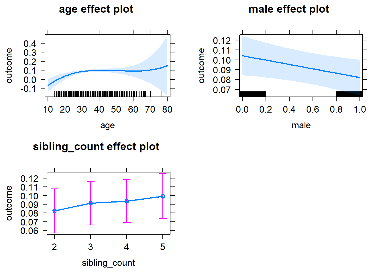
Add Birth Order Linear
Model Summary
tidy(m2_birthorder_linear, conf.int = T, conf.level = 0.995)| effect | group | term | estimate | std.error | statistic | df | p.value | conf.low | conf.high |
|---|---|---|---|---|---|---|---|---|---|
| fixed | NA | (Intercept) | -0.2384 | 0.07468 | -3.193 | 4590 | 0.00142 | -0.448 | -0.02879 |
| fixed | NA | birth_order | -0.00761 | 0.003611 | -2.108 | 4145 | 0.03513 | -0.01774 | 0.002526 |
| fixed | NA | poly(age, 3, raw = TRUE)1 | 0.02278 | 0.006695 | 3.402 | 4522 | 0.0006754 | 0.003982 | 0.04157 |
| fixed | NA | poly(age, 3, raw = TRUE)2 | -0.0004742 | 0.0001862 | -2.547 | 4423 | 0.01091 | -0.0009968 | 0.00004849 |
| fixed | NA | poly(age, 3, raw = TRUE)3 | 0.000003143 | 0.000001629 | 1.929 | 4337 | 0.05376 | -0.00000143 | 0.000007715 |
| fixed | NA | male | -0.02221 | 0.007446 | -2.983 | 4680 | 0.002869 | -0.04311 | -0.00131 |
| fixed | NA | sibling_count3 | 0.01176 | 0.01118 | 1.052 | 3636 | 0.293 | -0.01963 | 0.04315 |
| fixed | NA | sibling_count4 | 0.0171 | 0.01161 | 1.474 | 3712 | 0.1407 | -0.01548 | 0.04968 |
| fixed | NA | sibling_count5 | 0.02655 | 0.01263 | 2.102 | 3843 | 0.03561 | -0.008904 | 0.06201 |
| ran_pars | mother_pidlink | sd__(Intercept) | 0.12 | NA | NA | NA | NA | NA | NA |
| ran_pars | Residual | sd__Observation | 0.2311 | NA | NA | NA | NA | NA | NA |
Coefficient Plot
plot_birthorder2(m2_birthorder_linear, separate = FALSE)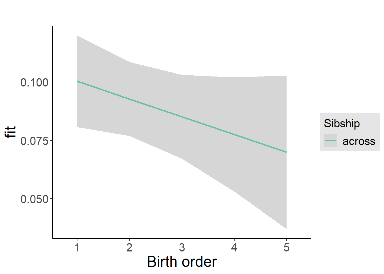
Add Birth Order Factor
Model Summary
m3_birthorder_nonlinear = update(m1_covariates_only, formula = . ~ . + birth_order_nonlinear)
tidy(m3_birthorder_nonlinear, conf.int = T, conf.level = 0.995)| effect | group | term | estimate | std.error | statistic | df | p.value | conf.low | conf.high |
|---|---|---|---|---|---|---|---|---|---|
| fixed | NA | (Intercept) | -0.2421 | 0.07487 | -3.233 | 4592 | 0.001232 | -0.4522 | -0.03192 |
| fixed | NA | poly(age, 3, raw = TRUE)1 | 0.02267 | 0.006697 | 3.385 | 4516 | 0.0007176 | 0.003871 | 0.04147 |
| fixed | NA | poly(age, 3, raw = TRUE)2 | -0.0004654 | 0.0001863 | -2.498 | 4413 | 0.01252 | -0.0009882 | 0.00005754 |
| fixed | NA | poly(age, 3, raw = TRUE)3 | 0.000003016 | 0.000001631 | 1.849 | 4320 | 0.06448 | -0.000001562 | 0.000007593 |
| fixed | NA | male | -0.02194 | 0.007448 | -2.946 | 4677 | 0.003234 | -0.04285 | -0.001036 |
| fixed | NA | sibling_count3 | 0.01291 | 0.01135 | 1.138 | 3767 | 0.2553 | -0.01894 | 0.04477 |
| fixed | NA | sibling_count4 | 0.01753 | 0.01178 | 1.488 | 3846 | 0.1368 | -0.01554 | 0.0506 |
| fixed | NA | sibling_count5 | 0.02368 | 0.01273 | 1.859 | 3923 | 0.06305 | -0.01207 | 0.05942 |
| fixed | NA | birth_order_nonlinear2 | -0.02111 | 0.008698 | -2.427 | 4102 | 0.01525 | -0.04553 | 0.003301 |
| fixed | NA | birth_order_nonlinear3 | -0.02331 | 0.01105 | -2.109 | 3992 | 0.03499 | -0.05433 | 0.007712 |
| fixed | NA | birth_order_nonlinear4 | -0.02374 | 0.01434 | -1.656 | 3919 | 0.09776 | -0.06399 | 0.0165 |
| fixed | NA | birth_order_nonlinear5 | -0.01536 | 0.02071 | -0.7416 | 3902 | 0.4583 | -0.0735 | 0.04278 |
| ran_pars | mother_pidlink | sd__(Intercept) | 0.1199 | NA | NA | NA | NA | NA | NA |
| ran_pars | Residual | sd__Observation | 0.2311 | NA | NA | NA | NA | NA | NA |
Coefficient Plot
plot_birthorder(m3_birthorder_nonlinear, separate = FALSE)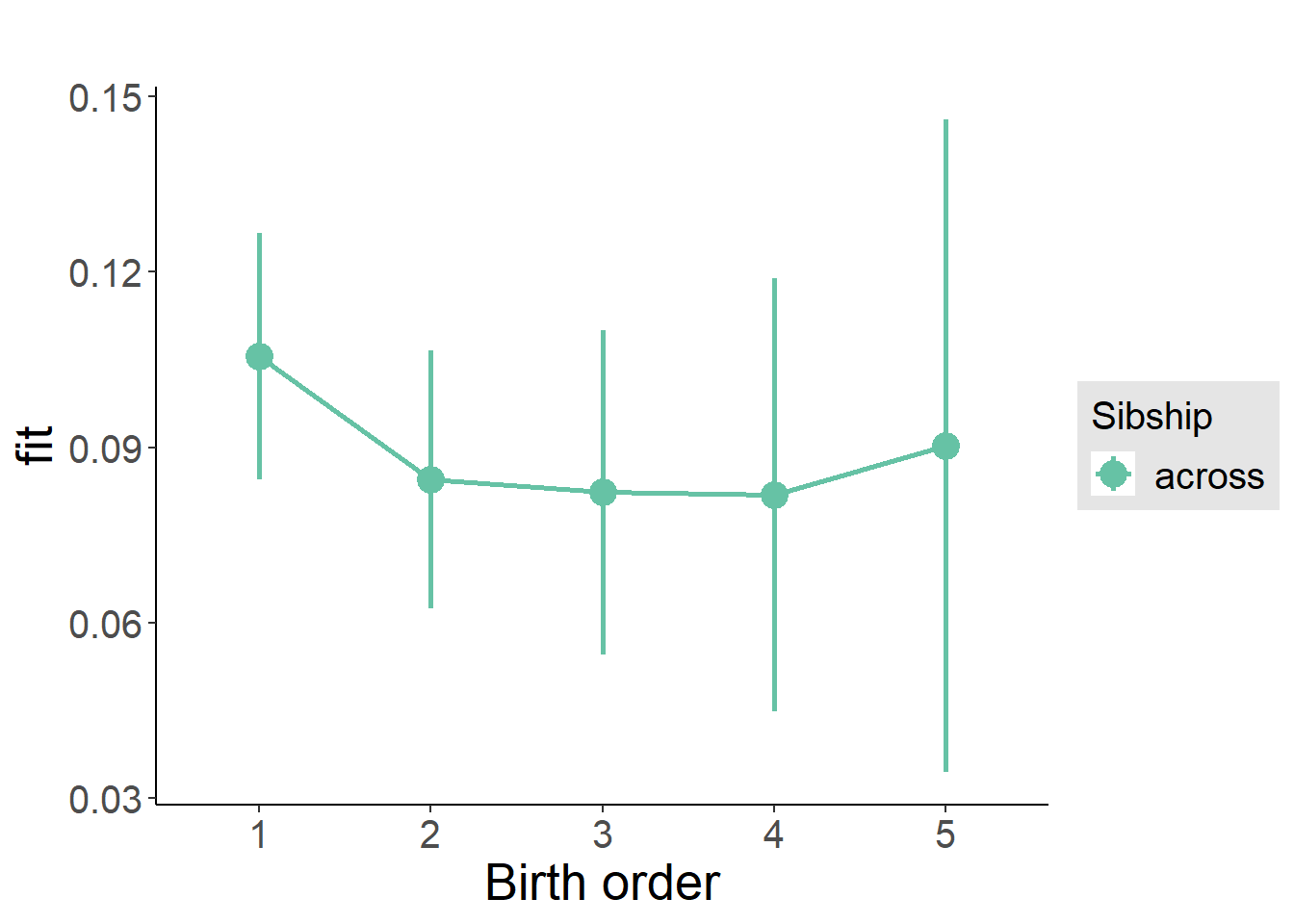
Add Interaction
Model Summary
m4_interaction = update(m3_birthorder_nonlinear, formula = . ~ . - birth_order_nonlinear - sibling_count + count_birth_order)
tidy(m4_interaction, conf.int = T, conf.level = 0.995)| effect | group | term | estimate | std.error | statistic | df | p.value | conf.low | conf.high |
|---|---|---|---|---|---|---|---|---|---|
| fixed | NA | (Intercept) | -0.2452 | 0.07499 | -3.27 | 4594 | 0.001084 | -0.4557 | -0.03471 |
| fixed | NA | poly(age, 3, raw = TRUE)1 | 0.02301 | 0.006703 | 3.432 | 4513 | 0.0006042 | 0.00419 | 0.04182 |
| fixed | NA | poly(age, 3, raw = TRUE)2 | -0.0004717 | 0.0001864 | -2.53 | 4410 | 0.01143 | -0.0009949 | 0.00005157 |
| fixed | NA | poly(age, 3, raw = TRUE)3 | 0.000003041 | 0.000001631 | 1.864 | 4316 | 0.06238 | -0.000001538 | 0.000007621 |
| fixed | NA | male | -0.02178 | 0.00745 | -2.924 | 4667 | 0.003475 | -0.04269 | -0.0008696 |
| fixed | NA | count_birth_order2/2 | -0.02547 | 0.01477 | -1.725 | 4099 | 0.08461 | -0.06693 | 0.01598 |
| fixed | NA | count_birth_order1/3 | 0.02047 | 0.01457 | 1.405 | 4781 | 0.1601 | -0.02044 | 0.06138 |
| fixed | NA | count_birth_order2/3 | -0.01757 | 0.01614 | -1.089 | 4803 | 0.2764 | -0.06287 | 0.02773 |
| fixed | NA | count_birth_order3/3 | -0.01937 | 0.01773 | -1.092 | 4804 | 0.2748 | -0.06914 | 0.03041 |
| fixed | NA | count_birth_order1/4 | 0.008919 | 0.01595 | 0.5591 | 4803 | 0.5761 | -0.03586 | 0.0537 |
| fixed | NA | count_birth_order2/4 | 0.01066 | 0.01709 | 0.6236 | 4806 | 0.5329 | -0.03732 | 0.05864 |
| fixed | NA | count_birth_order3/4 | -0.01085 | 0.01822 | -0.5957 | 4800 | 0.5514 | -0.06199 | 0.04028 |
| fixed | NA | count_birth_order4/4 | -0.01459 | 0.01937 | -0.7533 | 4793 | 0.4513 | -0.06897 | 0.03978 |
| fixed | NA | count_birth_order1/5 | 0.009719 | 0.01808 | 0.5376 | 4803 | 0.5909 | -0.04103 | 0.06047 |
| fixed | NA | count_birth_order2/5 | -0.004052 | 0.01918 | -0.2113 | 4796 | 0.8327 | -0.05788 | 0.04978 |
| fixed | NA | count_birth_order3/5 | 0.01331 | 0.02017 | 0.6599 | 4781 | 0.5094 | -0.04331 | 0.06993 |
| fixed | NA | count_birth_order4/5 | 0.006789 | 0.02118 | 0.3205 | 4739 | 0.7486 | -0.05266 | 0.06624 |
| fixed | NA | count_birth_order5/5 | 0.006999 | 0.02122 | 0.3299 | 4767 | 0.7415 | -0.05255 | 0.06655 |
| ran_pars | mother_pidlink | sd__(Intercept) | 0.1203 | NA | NA | NA | NA | NA | NA |
| ran_pars | Residual | sd__Observation | 0.2309 | NA | NA | NA | NA | NA | NA |
Coefficient Plot
plot_birthorder(m4_interaction)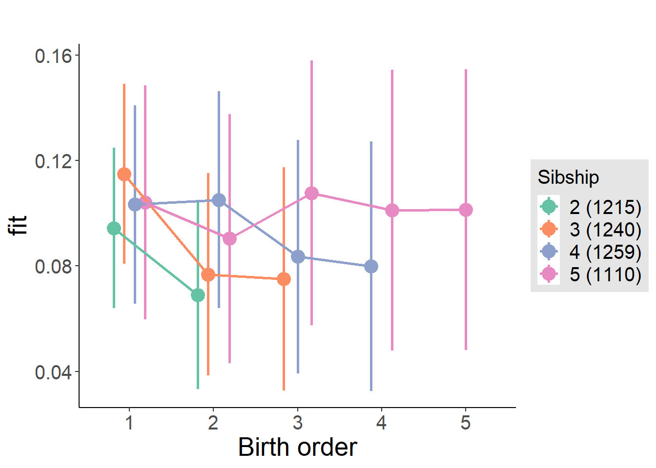
Model Comparison
###### Model 1 - Model 2
anova(m1_covariates_only, m2_birthorder_linear, m3_birthorder_nonlinear, m4_interaction)## refitting model(s) with ML (instead of REML)| Df | AIC | BIC | logLik | deviance | Chisq | Chi Df | Pr(>Chisq) |
|---|---|---|---|---|---|---|---|
| 10 | 636.2 | 701 | -308.1 | 616.2 | NA | NA | NA |
| 11 | 633.8 | 705.1 | -305.9 | 611.8 | 4.447 | 1 | 0.03497 |
| 14 | 636 | 726.8 | -304 | 608 | 3.745 | 3 | 0.2903 |
| 20 | 642.9 | 772.5 | -301.4 | 602.9 | 5.154 | 6 | 0.5242 |
Maternal birth order
outcome_uterus_m1 <- update(m2_birthorder_linear, data = birthorder %>%
mutate(sibling_count = sibling_count_uterus_alive_factor,
birth_order_nonlinear = birthorder_uterus_alive_factor,
birth_order = birthorder_uterus_alive,
count_birth_order = count_birthorder_uterus_alive) %>%
filter(sibling_count != "1"))
compare_models_markdown(outcome_uterus_m1)Basic Model
Model Summary
m1_covariates_only <- update(m2_birthorder_linear, formula = . ~ . - birth_order)
tidy(m1_covariates_only, conf.int = T, conf.level = 0.995)| effect | group | term | estimate | std.error | statistic | df | p.value | conf.low | conf.high |
|---|---|---|---|---|---|---|---|---|---|
| fixed | NA | (Intercept) | -0.8446 | 0.2218 | -3.808 | 2760 | 0.000143 | -1.467 | -0.222 |
| fixed | NA | poly(age, 3, raw = TRUE)1 | 0.08867 | 0.02457 | 3.609 | 2760 | 0.0003123 | 0.01971 | 0.1576 |
| fixed | NA | poly(age, 3, raw = TRUE)2 | -0.002752 | 0.0008712 | -3.159 | 2760 | 0.001599 | -0.005198 | -0.0003068 |
| fixed | NA | poly(age, 3, raw = TRUE)3 | 0.00002889 | 0.000009896 | 2.92 | 2760 | 0.003529 | 0.000001117 | 0.00005667 |
| fixed | NA | male | -0.01843 | 0.01034 | -1.782 | 2712 | 0.07488 | -0.04746 | 0.0106 |
| fixed | NA | sibling_count3 | 0.006876 | 0.01486 | 0.4628 | 2315 | 0.6435 | -0.03483 | 0.04858 |
| fixed | NA | sibling_count4 | 0.002255 | 0.01546 | 0.1459 | 2211 | 0.884 | -0.04114 | 0.04565 |
| fixed | NA | sibling_count5 | 0.001495 | 0.01727 | 0.08656 | 2046 | 0.931 | -0.047 | 0.04999 |
| ran_pars | mother_pidlink | sd__(Intercept) | 0.123 | NA | NA | NA | NA | NA | NA |
| ran_pars | Residual | sd__Observation | 0.242 | NA | NA | NA | NA | NA | NA |
Coefficient Plot
plot(allEffects(m1_covariates_only, confidence.level = 0.995))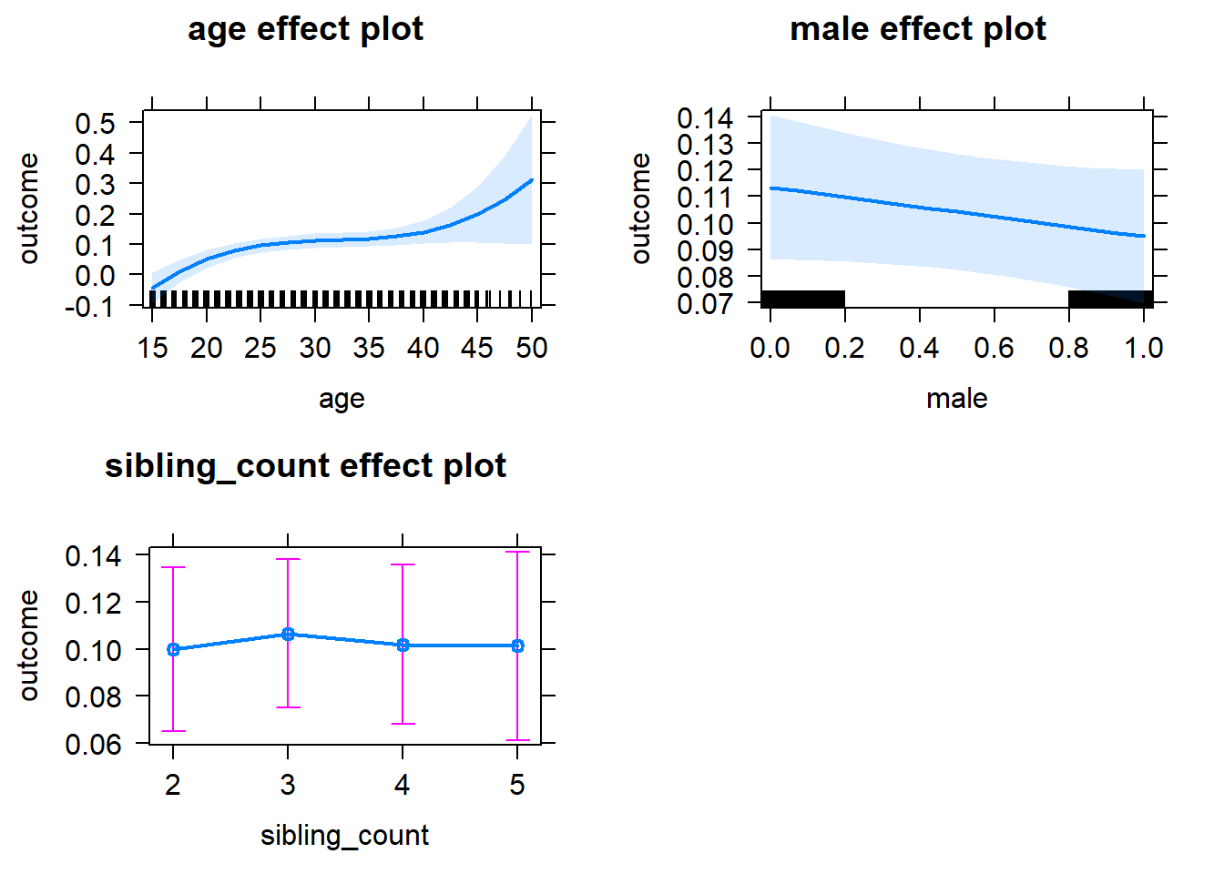
Add Birth Order Linear
Model Summary
tidy(m2_birthorder_linear, conf.int = T, conf.level = 0.995)| effect | group | term | estimate | std.error | statistic | df | p.value | conf.low | conf.high |
|---|---|---|---|---|---|---|---|---|---|
| fixed | NA | (Intercept) | -0.8437 | 0.2218 | -3.803 | 2759 | 0.0001458 | -1.466 | -0.221 |
| fixed | NA | birth_order | -0.002808 | 0.005173 | -0.5429 | 2605 | 0.5873 | -0.01733 | 0.01171 |
| fixed | NA | poly(age, 3, raw = TRUE)1 | 0.08891 | 0.02457 | 3.618 | 2759 | 0.0003018 | 0.01994 | 0.1579 |
| fixed | NA | poly(age, 3, raw = TRUE)2 | -0.002756 | 0.0008713 | -3.163 | 2759 | 0.001577 | -0.005202 | -0.0003104 |
| fixed | NA | poly(age, 3, raw = TRUE)3 | 0.00002886 | 0.000009897 | 2.916 | 2759 | 0.003573 | 0.000001079 | 0.00005664 |
| fixed | NA | male | -0.01842 | 0.01034 | -1.781 | 2711 | 0.07498 | -0.04746 | 0.01061 |
| fixed | NA | sibling_count3 | 0.008236 | 0.01507 | 0.5466 | 2339 | 0.5847 | -0.03406 | 0.05053 |
| fixed | NA | sibling_count4 | 0.005169 | 0.01636 | 0.3159 | 2305 | 0.7521 | -0.04077 | 0.05111 |
| fixed | NA | sibling_count5 | 0.006382 | 0.01948 | 0.3276 | 2296 | 0.7433 | -0.04831 | 0.06107 |
| ran_pars | mother_pidlink | sd__(Intercept) | 0.1228 | NA | NA | NA | NA | NA | NA |
| ran_pars | Residual | sd__Observation | 0.2421 | NA | NA | NA | NA | NA | NA |
Coefficient Plot
plot_birthorder2(m2_birthorder_linear, separate = FALSE)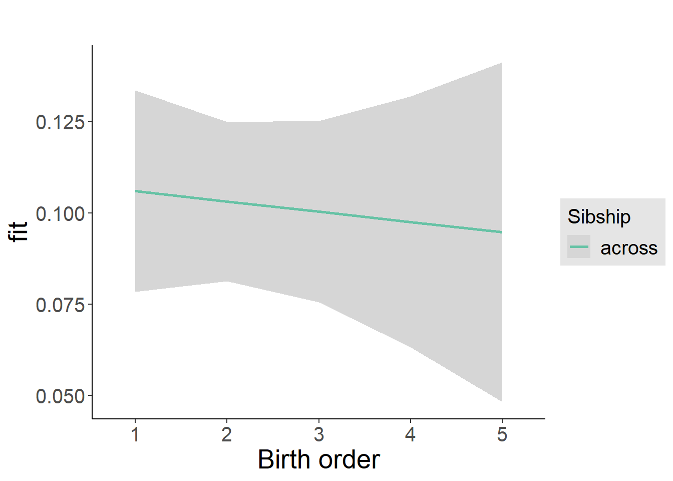
Add Birth Order Factor
Model Summary
m3_birthorder_nonlinear = update(m1_covariates_only, formula = . ~ . + birth_order_nonlinear)
tidy(m3_birthorder_nonlinear, conf.int = T, conf.level = 0.995)| effect | group | term | estimate | std.error | statistic | df | p.value | conf.low | conf.high |
|---|---|---|---|---|---|---|---|---|---|
| fixed | NA | (Intercept) | -0.8255 | 0.2223 | -3.713 | 2756 | 0.0002088 | -1.45 | -0.2014 |
| fixed | NA | poly(age, 3, raw = TRUE)1 | 0.08702 | 0.02462 | 3.535 | 2756 | 0.0004143 | 0.01792 | 0.1561 |
| fixed | NA | poly(age, 3, raw = TRUE)2 | -0.002688 | 0.0008728 | -3.079 | 2756 | 0.002094 | -0.005138 | -0.0002378 |
| fixed | NA | poly(age, 3, raw = TRUE)3 | 0.00002811 | 0.000009913 | 2.836 | 2756 | 0.004604 | 0.0000002856 | 0.00005594 |
| fixed | NA | male | -0.01883 | 0.01035 | -1.82 | 2708 | 0.06892 | -0.04788 | 0.01022 |
| fixed | NA | sibling_count3 | 0.01055 | 0.01528 | 0.6901 | 2383 | 0.4902 | -0.03235 | 0.05344 |
| fixed | NA | sibling_count4 | 0.004998 | 0.01656 | 0.3018 | 2346 | 0.7629 | -0.0415 | 0.05149 |
| fixed | NA | sibling_count5 | 0.002295 | 0.01972 | 0.1164 | 2328 | 0.9074 | -0.05305 | 0.05764 |
| fixed | NA | birth_order_nonlinear2 | -0.01815 | 0.01226 | -1.48 | 2386 | 0.139 | -0.05257 | 0.01627 |
| fixed | NA | birth_order_nonlinear3 | -0.01674 | 0.015 | -1.116 | 2432 | 0.2644 | -0.05883 | 0.02535 |
| fixed | NA | birth_order_nonlinear4 | -0.0002889 | 0.01995 | -0.01448 | 2482 | 0.9885 | -0.0563 | 0.05572 |
| fixed | NA | birth_order_nonlinear5 | -0.000882 | 0.03059 | -0.02883 | 2415 | 0.977 | -0.08676 | 0.085 |
| ran_pars | mother_pidlink | sd__(Intercept) | 0.1233 | NA | NA | NA | NA | NA | NA |
| ran_pars | Residual | sd__Observation | 0.2419 | NA | NA | NA | NA | NA | NA |
Coefficient Plot
plot_birthorder(m3_birthorder_nonlinear, separate = FALSE)
Add Interaction
Model Summary
m4_interaction = update(m3_birthorder_nonlinear, formula = . ~ . - birth_order_nonlinear - sibling_count + count_birth_order)
tidy(m4_interaction, conf.int = T, conf.level = 0.995)| effect | group | term | estimate | std.error | statistic | df | p.value | conf.low | conf.high |
|---|---|---|---|---|---|---|---|---|---|
| fixed | NA | (Intercept) | -0.8108 | 0.2224 | -3.646 | 2750 | 0.0002716 | -1.435 | -0.1865 |
| fixed | NA | poly(age, 3, raw = TRUE)1 | 0.08584 | 0.02462 | 3.486 | 2750 | 0.0004981 | 0.01672 | 0.155 |
| fixed | NA | poly(age, 3, raw = TRUE)2 | -0.002651 | 0.0008732 | -3.036 | 2750 | 0.002421 | -0.005102 | -0.0001998 |
| fixed | NA | poly(age, 3, raw = TRUE)3 | 0.00002775 | 0.000009919 | 2.798 | 2750 | 0.005179 | -0.00000009005 | 0.00005559 |
| fixed | NA | male | -0.01918 | 0.01036 | -1.851 | 2701 | 0.06424 | -0.04826 | 0.009901 |
| fixed | NA | count_birth_order2/2 | -0.0267 | 0.02229 | -1.198 | 2458 | 0.231 | -0.08926 | 0.03586 |
| fixed | NA | count_birth_order1/3 | 0.01513 | 0.01917 | 0.7894 | 2744 | 0.4299 | -0.03867 | 0.06893 |
| fixed | NA | count_birth_order2/3 | -0.01745 | 0.02124 | -0.8216 | 2750 | 0.4114 | -0.07709 | 0.04218 |
| fixed | NA | count_birth_order3/3 | -0.01395 | 0.02296 | -0.6075 | 2746 | 0.5436 | -0.07838 | 0.05049 |
| fixed | NA | count_birth_order1/4 | -0.01733 | 0.02206 | -0.7856 | 2750 | 0.4321 | -0.07924 | 0.04459 |
| fixed | NA | count_birth_order2/4 | 0.007161 | 0.02313 | 0.3097 | 2747 | 0.7568 | -0.05776 | 0.07208 |
| fixed | NA | count_birth_order3/4 | 0.001317 | 0.02421 | 0.05438 | 2736 | 0.9566 | -0.06665 | 0.06928 |
| fixed | NA | count_birth_order4/4 | -0.01636 | 0.02565 | -0.6378 | 2732 | 0.5237 | -0.08835 | 0.05564 |
| fixed | NA | count_birth_order1/5 | 0.006228 | 0.02895 | 0.2151 | 2746 | 0.8297 | -0.07504 | 0.08749 |
| fixed | NA | count_birth_order2/5 | -0.03768 | 0.03135 | -1.202 | 2713 | 0.2295 | -0.1257 | 0.05032 |
| fixed | NA | count_birth_order3/5 | -0.03459 | 0.02935 | -1.179 | 2720 | 0.2387 | -0.117 | 0.04779 |
| fixed | NA | count_birth_order4/5 | 0.02366 | 0.02851 | 0.83 | 2718 | 0.4066 | -0.05637 | 0.1037 |
| fixed | NA | count_birth_order5/5 | -0.001001 | 0.02988 | -0.03349 | 2712 | 0.9733 | -0.08486 | 0.08286 |
| ran_pars | mother_pidlink | sd__(Intercept) | 0.1233 | NA | NA | NA | NA | NA | NA |
| ran_pars | Residual | sd__Observation | 0.2418 | NA | NA | NA | NA | NA | NA |
Coefficient Plot
plot_birthorder(m4_interaction)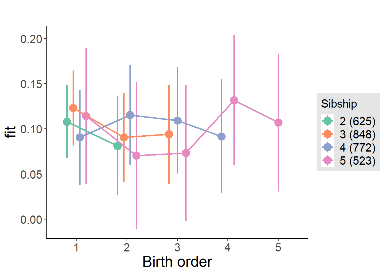
Model Comparison
###### Model 1 - Model 2
anova(m1_covariates_only, m2_birthorder_linear, m3_birthorder_nonlinear, m4_interaction)## refitting model(s) with ML (instead of REML)| Df | AIC | BIC | logLik | deviance | Chisq | Chi Df | Pr(>Chisq) |
|---|---|---|---|---|---|---|---|
| 10 | 611.1 | 670.4 | -295.6 | 591.1 | NA | NA | NA |
| 11 | 612.8 | 678 | -295.4 | 590.8 | 0.2966 | 1 | 0.586 |
| 14 | 616.1 | 699.1 | -294.1 | 588.1 | 2.706 | 3 | 0.4392 |
| 20 | 620.9 | 739.5 | -290.5 | 580.9 | 7.19 | 6 | 0.3036 |
Maternal pregnancy order
outcome_preg_m1 <- update(m2_birthorder_linear, data = birthorder %>%
mutate(sibling_count = sibling_count_uterus_preg_factor,
birth_order_nonlinear = birthorder_uterus_preg_factor,
birth_order = birthorder_uterus_preg,
count_birth_order = count_birthorder_uterus_preg
) %>%
filter(sibling_count != "1"))
compare_models_markdown(outcome_preg_m1)Basic Model
Model Summary
m1_covariates_only <- update(m2_birthorder_linear, formula = . ~ . - birth_order)
tidy(m1_covariates_only, conf.int = T, conf.level = 0.995)| effect | group | term | estimate | std.error | statistic | df | p.value | conf.low | conf.high |
|---|---|---|---|---|---|---|---|---|---|
| fixed | NA | (Intercept) | -0.8203 | 0.228 | -3.598 | 2531 | 0.0003268 | -1.46 | -0.1803 |
| fixed | NA | poly(age, 3, raw = TRUE)1 | 0.08539 | 0.02527 | 3.38 | 2530 | 0.0007366 | 0.01447 | 0.1563 |
| fixed | NA | poly(age, 3, raw = TRUE)2 | -0.002664 | 0.000896 | -2.973 | 2530 | 0.002975 | -0.005179 | -0.0001489 |
| fixed | NA | poly(age, 3, raw = TRUE)3 | 0.00002825 | 0.00001018 | 2.775 | 2530 | 0.005558 | -0.0000003247 | 0.00005682 |
| fixed | NA | male | -0.01378 | 0.01073 | -1.284 | 2492 | 0.1992 | -0.04388 | 0.01633 |
| fixed | NA | sibling_count3 | 0.008393 | 0.01615 | 0.5198 | 2181 | 0.6033 | -0.03693 | 0.05372 |
| fixed | NA | sibling_count4 | 0.01724 | 0.01638 | 1.053 | 2121 | 0.2925 | -0.02873 | 0.06322 |
| fixed | NA | sibling_count5 | 0.01254 | 0.01734 | 0.7233 | 2024 | 0.4696 | -0.03612 | 0.0612 |
| ran_pars | mother_pidlink | sd__(Intercept) | 0.1219 | NA | NA | NA | NA | NA | NA |
| ran_pars | Residual | sd__Observation | 0.2402 | NA | NA | NA | NA | NA | NA |
Coefficient Plot
plot(allEffects(m1_covariates_only, confidence.level = 0.995))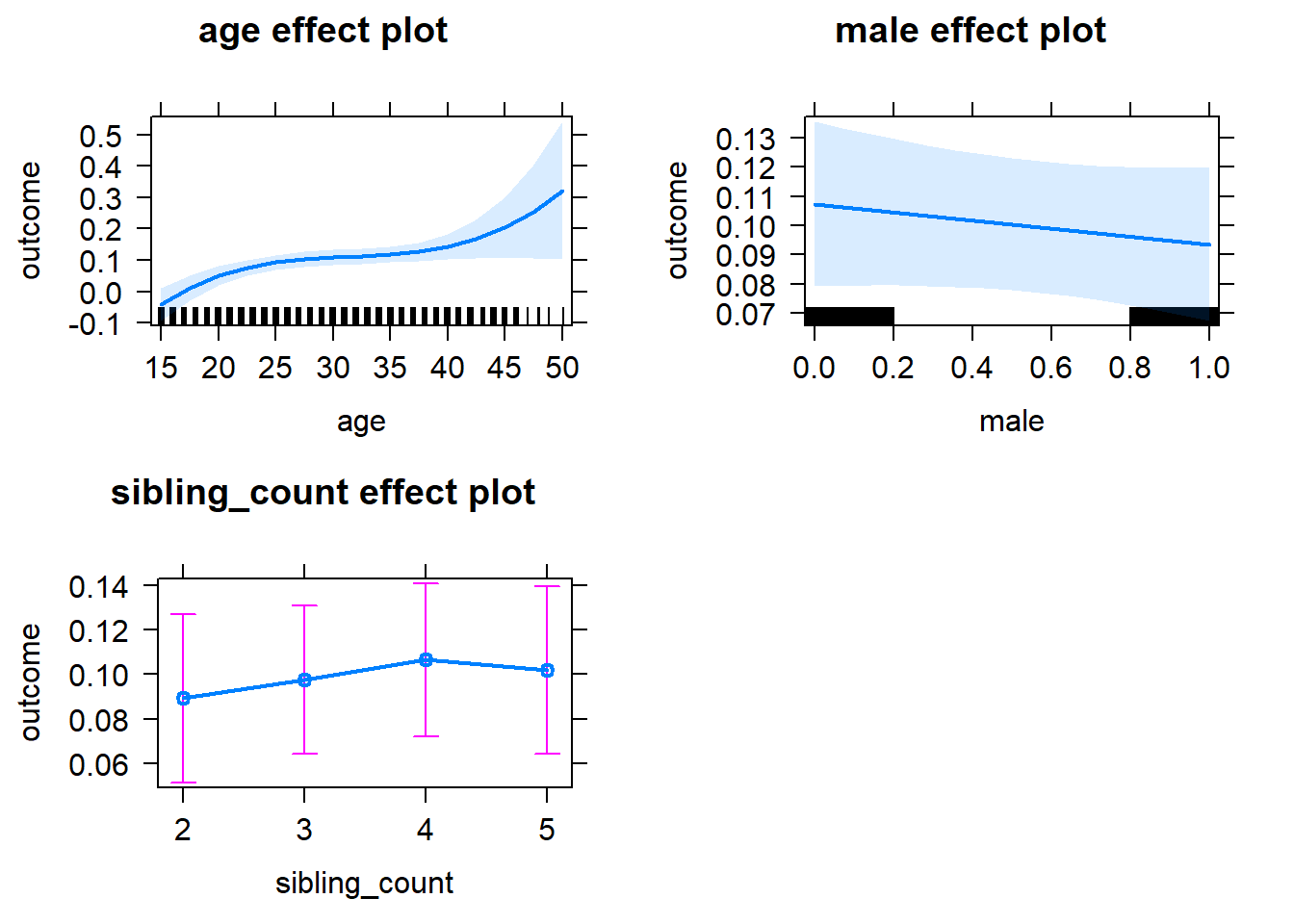
Add Birth Order Linear
Model Summary
tidy(m2_birthorder_linear, conf.int = T, conf.level = 0.995)| effect | group | term | estimate | std.error | statistic | df | p.value | conf.low | conf.high |
|---|---|---|---|---|---|---|---|---|---|
| fixed | NA | (Intercept) | -0.815 | 0.228 | -3.574 | 2530 | 0.0003577 | -1.455 | -0.1749 |
| fixed | NA | birth_order | -0.006519 | 0.005213 | -1.251 | 2434 | 0.2112 | -0.02115 | 0.008113 |
| fixed | NA | poly(age, 3, raw = TRUE)1 | 0.0857 | 0.02527 | 3.392 | 2530 | 0.0007049 | 0.01478 | 0.1566 |
| fixed | NA | poly(age, 3, raw = TRUE)2 | -0.002667 | 0.0008959 | -2.977 | 2529 | 0.002942 | -0.005182 | -0.000152 |
| fixed | NA | poly(age, 3, raw = TRUE)3 | 0.00002812 | 0.00001018 | 2.763 | 2529 | 0.005767 | -0.0000004469 | 0.00005669 |
| fixed | NA | male | -0.01396 | 0.01073 | -1.302 | 2491 | 0.1932 | -0.04407 | 0.01615 |
| fixed | NA | sibling_count3 | 0.01165 | 0.01635 | 0.7127 | 2194 | 0.4761 | -0.03424 | 0.05755 |
| fixed | NA | sibling_count4 | 0.0236 | 0.01714 | 1.377 | 2174 | 0.1687 | -0.02452 | 0.07171 |
| fixed | NA | sibling_count5 | 0.02314 | 0.01929 | 1.2 | 2184 | 0.2304 | -0.03101 | 0.07729 |
| ran_pars | mother_pidlink | sd__(Intercept) | 0.1214 | NA | NA | NA | NA | NA | NA |
| ran_pars | Residual | sd__Observation | 0.2403 | NA | NA | NA | NA | NA | NA |
Coefficient Plot
plot_birthorder2(m2_birthorder_linear, separate = FALSE)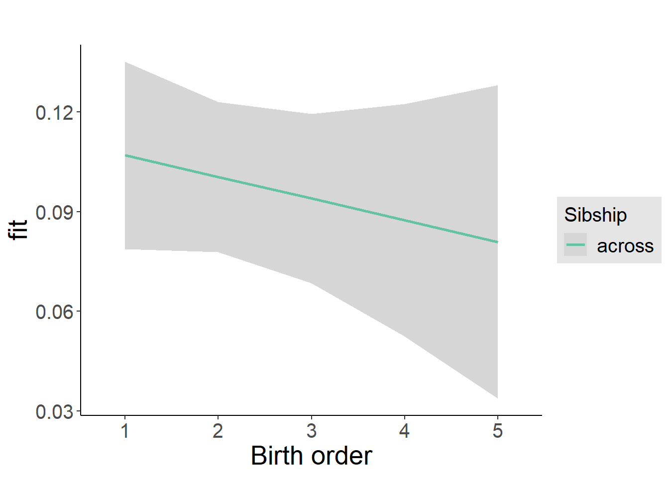
Add Birth Order Factor
Model Summary
m3_birthorder_nonlinear = update(m1_covariates_only, formula = . ~ . + birth_order_nonlinear)
tidy(m3_birthorder_nonlinear, conf.int = T, conf.level = 0.995)| effect | group | term | estimate | std.error | statistic | df | p.value | conf.low | conf.high |
|---|---|---|---|---|---|---|---|---|---|
| fixed | NA | (Intercept) | -0.7987 | 0.2285 | -3.495 | 2527 | 0.0004817 | -1.44 | -0.1573 |
| fixed | NA | poly(age, 3, raw = TRUE)1 | 0.08338 | 0.02532 | 3.293 | 2527 | 0.001003 | 0.01232 | 0.1544 |
| fixed | NA | poly(age, 3, raw = TRUE)2 | -0.002584 | 0.0008978 | -2.878 | 2527 | 0.004036 | -0.005104 | -0.00006367 |
| fixed | NA | poly(age, 3, raw = TRUE)3 | 0.00002721 | 0.0000102 | 2.668 | 2527 | 0.007676 | -0.000001416 | 0.00005583 |
| fixed | NA | male | -0.01452 | 0.01073 | -1.353 | 2486 | 0.1761 | -0.04462 | 0.01559 |
| fixed | NA | sibling_count3 | 0.01511 | 0.01657 | 0.9116 | 2225 | 0.3621 | -0.03142 | 0.06164 |
| fixed | NA | sibling_count4 | 0.02174 | 0.01734 | 1.253 | 2202 | 0.2102 | -0.02694 | 0.07041 |
| fixed | NA | sibling_count5 | 0.02271 | 0.01941 | 1.17 | 2196 | 0.2421 | -0.03177 | 0.0772 |
| fixed | NA | birth_order_nonlinear2 | -0.01468 | 0.01265 | -1.16 | 2224 | 0.246 | -0.05018 | 0.02083 |
| fixed | NA | birth_order_nonlinear3 | -0.02852 | 0.01563 | -1.824 | 2287 | 0.06822 | -0.0724 | 0.01536 |
| fixed | NA | birth_order_nonlinear4 | 0.006131 | 0.02052 | 0.2988 | 2320 | 0.7651 | -0.05147 | 0.06373 |
| fixed | NA | birth_order_nonlinear5 | -0.04046 | 0.02928 | -1.382 | 2262 | 0.1672 | -0.1226 | 0.04173 |
| ran_pars | mother_pidlink | sd__(Intercept) | 0.1227 | NA | NA | NA | NA | NA | NA |
| ran_pars | Residual | sd__Observation | 0.2397 | NA | NA | NA | NA | NA | NA |
Coefficient Plot
plot_birthorder(m3_birthorder_nonlinear, separate = FALSE)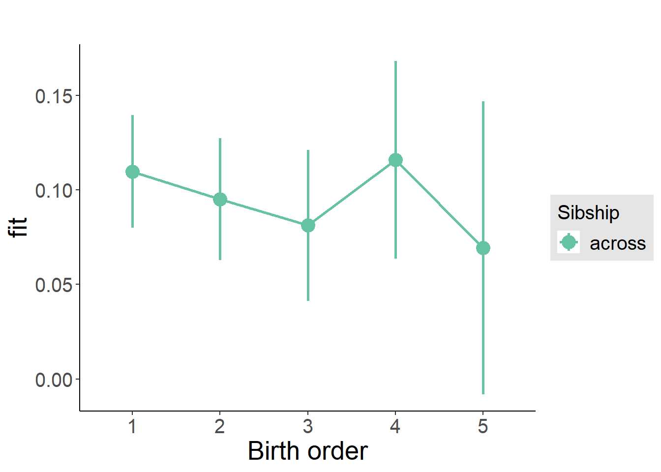
Add Interaction
Model Summary
m4_interaction = update(m3_birthorder_nonlinear, formula = . ~ . - birth_order_nonlinear - sibling_count + count_birth_order)
tidy(m4_interaction, conf.int = T, conf.level = 0.995)| effect | group | term | estimate | std.error | statistic | df | p.value | conf.low | conf.high |
|---|---|---|---|---|---|---|---|---|---|
| fixed | NA | (Intercept) | -0.7886 | 0.2283 | -3.454 | 2521 | 0.0005614 | -1.43 | -0.1477 |
| fixed | NA | poly(age, 3, raw = TRUE)1 | 0.08258 | 0.0253 | 3.265 | 2521 | 0.00111 | 0.01158 | 0.1536 |
| fixed | NA | poly(age, 3, raw = TRUE)2 | -0.002554 | 0.000897 | -2.847 | 2521 | 0.004442 | -0.005072 | -0.00003629 |
| fixed | NA | poly(age, 3, raw = TRUE)3 | 0.00002686 | 0.00001019 | 2.636 | 2521 | 0.008452 | -0.000001748 | 0.00005546 |
| fixed | NA | male | -0.01525 | 0.01073 | -1.421 | 2479 | 0.1554 | -0.04536 | 0.01487 |
| fixed | NA | count_birth_order2/2 | -0.02294 | 0.02433 | -0.943 | 2321 | 0.3458 | -0.09122 | 0.04534 |
| fixed | NA | count_birth_order1/3 | 0.0179 | 0.02099 | 0.8529 | 2516 | 0.3938 | -0.04102 | 0.07682 |
| fixed | NA | count_birth_order2/3 | -0.01219 | 0.02278 | -0.5351 | 2521 | 0.5926 | -0.07613 | 0.05175 |
| fixed | NA | count_birth_order3/3 | -0.01276 | 0.02501 | -0.5102 | 2517 | 0.6099 | -0.08297 | 0.05745 |
| fixed | NA | count_birth_order1/4 | 0.006472 | 0.02288 | 0.2828 | 2520 | 0.7773 | -0.05775 | 0.0707 |
| fixed | NA | count_birth_order2/4 | 0.0439 | 0.02381 | 1.844 | 2520 | 0.06535 | -0.02294 | 0.1107 |
| fixed | NA | count_birth_order3/4 | -0.01099 | 0.02596 | -0.4231 | 2508 | 0.6723 | -0.08387 | 0.0619 |
| fixed | NA | count_birth_order4/4 | -0.01307 | 0.02767 | -0.4725 | 2503 | 0.6366 | -0.09075 | 0.0646 |
| fixed | NA | count_birth_order1/5 | 0.0234 | 0.02743 | 0.8532 | 2520 | 0.3937 | -0.0536 | 0.1004 |
| fixed | NA | count_birth_order2/5 | -0.03431 | 0.02841 | -1.208 | 2510 | 0.2273 | -0.1141 | 0.04544 |
| fixed | NA | count_birth_order3/5 | -0.01171 | 0.02885 | -0.406 | 2499 | 0.6848 | -0.09271 | 0.06928 |
| fixed | NA | count_birth_order4/5 | 0.07044 | 0.02926 | 2.408 | 2488 | 0.01613 | -0.01169 | 0.1526 |
| fixed | NA | count_birth_order5/5 | -0.01972 | 0.02947 | -0.6693 | 2488 | 0.5034 | -0.1024 | 0.063 |
| ran_pars | mother_pidlink | sd__(Intercept) | 0.1229 | NA | NA | NA | NA | NA | NA |
| ran_pars | Residual | sd__Observation | 0.2391 | NA | NA | NA | NA | NA | NA |
Coefficient Plot
plot_birthorder(m4_interaction)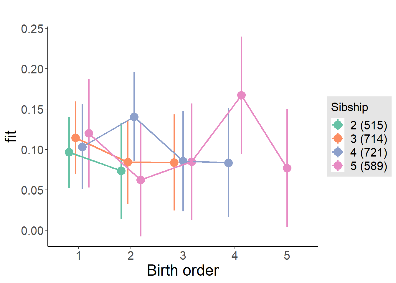
Model Comparison
###### Model 1 - Model 2
anova(m1_covariates_only, m2_birthorder_linear, m3_birthorder_nonlinear, m4_interaction)## refitting model(s) with ML (instead of REML)| Df | AIC | BIC | logLik | deviance | Chisq | Chi Df | Pr(>Chisq) |
|---|---|---|---|---|---|---|---|
| 10 | 523.2 | 581.6 | -251.6 | 503.2 | NA | NA | NA |
| 11 | 523.7 | 587.9 | -250.8 | 501.7 | 1.57 | 1 | 0.2103 |
| 14 | 525.3 | 607 | -248.6 | 497.3 | 4.389 | 3 | 0.2224 |
| 20 | 522.3 | 639.1 | -241.1 | 482.3 | 14.97 | 6 | 0.02049 |
Parental full sibling order
outcome_parental_m1 <- update(m2_birthorder_linear, data = birthorder %>%
mutate(sibling_count = sibling_count_genes_factor,
birth_order_nonlinear = birthorder_genes_factor,
birth_order = birthorder_genes,
count_birth_order = count_birthorder_genes
) %>%
filter(sibling_count != "1"))
compare_models_markdown(outcome_parental_m1)Basic Model
Model Summary
m1_covariates_only <- update(m2_birthorder_linear, formula = . ~ . - birth_order)
tidy(m1_covariates_only, conf.int = T, conf.level = 0.995)| effect | group | term | estimate | std.error | statistic | df | p.value | conf.low | conf.high |
|---|---|---|---|---|---|---|---|---|---|
| fixed | NA | (Intercept) | -0.9011 | 0.2241 | -4.021 | 2760 | 0.00005945 | -1.53 | -0.2721 |
| fixed | NA | poly(age, 3, raw = TRUE)1 | 0.09554 | 0.02488 | 3.839 | 2760 | 0.0001261 | 0.02569 | 0.1654 |
| fixed | NA | poly(age, 3, raw = TRUE)2 | -0.003015 | 0.0008845 | -3.408 | 2760 | 0.0006628 | -0.005497 | -0.0005319 |
| fixed | NA | poly(age, 3, raw = TRUE)3 | 0.00003197 | 0.00001007 | 3.174 | 2760 | 0.001522 | 0.000003693 | 0.00006024 |
| fixed | NA | male | -0.01993 | 0.01034 | -1.928 | 2710 | 0.05392 | -0.04894 | 0.009082 |
| fixed | NA | sibling_count3 | 0.005211 | 0.01457 | 0.3576 | 2325 | 0.7206 | -0.03569 | 0.04611 |
| fixed | NA | sibling_count4 | 0.009886 | 0.01537 | 0.6433 | 2216 | 0.5201 | -0.03325 | 0.05302 |
| fixed | NA | sibling_count5 | 0.007623 | 0.01767 | 0.4313 | 2004 | 0.6663 | -0.04199 | 0.05723 |
| ran_pars | mother_pidlink | sd__(Intercept) | 0.1241 | NA | NA | NA | NA | NA | NA |
| ran_pars | Residual | sd__Observation | 0.2414 | NA | NA | NA | NA | NA | NA |
Coefficient Plot
plot(allEffects(m1_covariates_only, confidence.level = 0.995))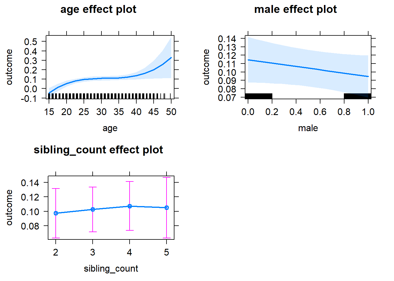
Add Birth Order Linear
Model Summary
tidy(m2_birthorder_linear, conf.int = T, conf.level = 0.995)| effect | group | term | estimate | std.error | statistic | df | p.value | conf.low | conf.high |
|---|---|---|---|---|---|---|---|---|---|
| fixed | NA | (Intercept) | -0.9001 | 0.2241 | -4.016 | 2759 | 0.00006069 | -1.529 | -0.271 |
| fixed | NA | birth_order | -0.002497 | 0.005229 | -0.4776 | 2587 | 0.633 | -0.01718 | 0.01218 |
| fixed | NA | poly(age, 3, raw = TRUE)1 | 0.09575 | 0.02489 | 3.847 | 2759 | 0.0001224 | 0.02588 | 0.1656 |
| fixed | NA | poly(age, 3, raw = TRUE)2 | -0.003018 | 0.0008846 | -3.412 | 2759 | 0.0006545 | -0.005501 | -0.000535 |
| fixed | NA | poly(age, 3, raw = TRUE)3 | 0.00003194 | 0.00001007 | 3.17 | 2759 | 0.001539 | 0.000003661 | 0.00006022 |
| fixed | NA | male | -0.01995 | 0.01034 | -1.93 | 2709 | 0.0537 | -0.04897 | 0.009065 |
| fixed | NA | sibling_count3 | 0.006438 | 0.0148 | 0.4351 | 2347 | 0.6635 | -0.0351 | 0.04797 |
| fixed | NA | sibling_count4 | 0.01244 | 0.01628 | 0.7646 | 2314 | 0.4446 | -0.03324 | 0.05813 |
| fixed | NA | sibling_count5 | 0.01183 | 0.01975 | 0.599 | 2237 | 0.5492 | -0.04361 | 0.06727 |
| ran_pars | mother_pidlink | sd__(Intercept) | 0.1239 | NA | NA | NA | NA | NA | NA |
| ran_pars | Residual | sd__Observation | 0.2415 | NA | NA | NA | NA | NA | NA |
Coefficient Plot
plot_birthorder2(m2_birthorder_linear, separate = FALSE)
Add Birth Order Factor
Model Summary
m3_birthorder_nonlinear = update(m1_covariates_only, formula = . ~ . + birth_order_nonlinear)
tidy(m3_birthorder_nonlinear, conf.int = T, conf.level = 0.995)| effect | group | term | estimate | std.error | statistic | df | p.value | conf.low | conf.high |
|---|---|---|---|---|---|---|---|---|---|
| fixed | NA | (Intercept) | -0.8845 | 0.2246 | -3.939 | 2756 | 0.00008394 | -1.515 | -0.2541 |
| fixed | NA | poly(age, 3, raw = TRUE)1 | 0.09407 | 0.02493 | 3.773 | 2756 | 0.000165 | 0.02408 | 0.1641 |
| fixed | NA | poly(age, 3, raw = TRUE)2 | -0.002958 | 0.0008861 | -3.338 | 2756 | 0.0008561 | -0.005445 | -0.0004702 |
| fixed | NA | poly(age, 3, raw = TRUE)3 | 0.00003128 | 0.00001009 | 3.1 | 2756 | 0.001953 | 0.000002958 | 0.0000596 |
| fixed | NA | male | -0.0203 | 0.01035 | -1.962 | 2706 | 0.04985 | -0.04934 | 0.008742 |
| fixed | NA | sibling_count3 | 0.008672 | 0.01501 | 0.5775 | 2392 | 0.5636 | -0.03348 | 0.05082 |
| fixed | NA | sibling_count4 | 0.01184 | 0.01648 | 0.7184 | 2355 | 0.4726 | -0.03441 | 0.05809 |
| fixed | NA | sibling_count5 | 0.008193 | 0.02006 | 0.4085 | 2281 | 0.683 | -0.04811 | 0.06449 |
| fixed | NA | birth_order_nonlinear2 | -0.01399 | 0.01212 | -1.154 | 2370 | 0.2486 | -0.04801 | 0.02003 |
| fixed | NA | birth_order_nonlinear3 | -0.0158 | 0.01495 | -1.057 | 2424 | 0.2905 | -0.05775 | 0.02615 |
| fixed | NA | birth_order_nonlinear4 | 0.004316 | 0.02048 | 0.2108 | 2465 | 0.8331 | -0.05316 | 0.0618 |
| fixed | NA | birth_order_nonlinear5 | -0.00392 | 0.03223 | -0.1216 | 2410 | 0.9032 | -0.0944 | 0.08656 |
| ran_pars | mother_pidlink | sd__(Intercept) | 0.1243 | NA | NA | NA | NA | NA | NA |
| ran_pars | Residual | sd__Observation | 0.2414 | NA | NA | NA | NA | NA | NA |
Coefficient Plot
plot_birthorder(m3_birthorder_nonlinear, separate = FALSE)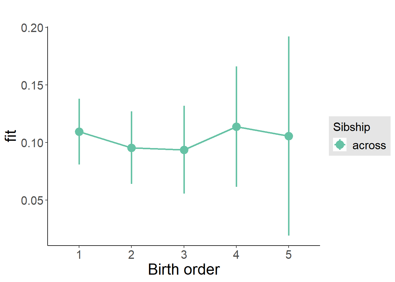
Add Interaction
Model Summary
m4_interaction = update(m3_birthorder_nonlinear, formula = . ~ . - birth_order_nonlinear - sibling_count + count_birth_order)
tidy(m4_interaction, conf.int = T, conf.level = 0.995)| effect | group | term | estimate | std.error | statistic | df | p.value | conf.low | conf.high |
|---|---|---|---|---|---|---|---|---|---|
| fixed | NA | (Intercept) | -0.8709 | 0.2247 | -3.876 | 2750 | 0.0001085 | -1.502 | -0.2402 |
| fixed | NA | poly(age, 3, raw = TRUE)1 | 0.09326 | 0.02495 | 3.738 | 2750 | 0.000189 | 0.02323 | 0.1633 |
| fixed | NA | poly(age, 3, raw = TRUE)2 | -0.002939 | 0.0008867 | -3.314 | 2750 | 0.0009308 | -0.005428 | -0.0004497 |
| fixed | NA | poly(age, 3, raw = TRUE)3 | 0.00003119 | 0.0000101 | 3.089 | 2750 | 0.002029 | 0.000002846 | 0.00005954 |
| fixed | NA | male | -0.02027 | 0.01036 | -1.958 | 2699 | 0.05039 | -0.04934 | 0.008797 |
| fixed | NA | count_birth_order2/2 | -0.02733 | 0.02163 | -1.264 | 2435 | 0.2065 | -0.08804 | 0.03338 |
| fixed | NA | count_birth_order1/3 | 0.01519 | 0.01885 | 0.8061 | 2744 | 0.4203 | -0.03771 | 0.0681 |
| fixed | NA | count_birth_order2/3 | -0.01803 | 0.0209 | -0.8624 | 2749 | 0.3885 | -0.07671 | 0.04065 |
| fixed | NA | count_birth_order3/3 | -0.02169 | 0.02235 | -0.9705 | 2743 | 0.3319 | -0.08445 | 0.04106 |
| fixed | NA | count_birth_order1/4 | -0.01651 | 0.02213 | -0.7459 | 2750 | 0.4558 | -0.07864 | 0.04562 |
| fixed | NA | count_birth_order2/4 | 0.01695 | 0.02305 | 0.7352 | 2745 | 0.4623 | -0.04776 | 0.08166 |
| fixed | NA | count_birth_order3/4 | 0.003404 | 0.02413 | 0.1411 | 2734 | 0.8878 | -0.06432 | 0.07113 |
| fixed | NA | count_birth_order4/4 | 0.003352 | 0.02598 | 0.129 | 2728 | 0.8974 | -0.06958 | 0.07629 |
| fixed | NA | count_birth_order1/5 | -0.003096 | 0.02898 | -0.1068 | 2747 | 0.9149 | -0.08444 | 0.07825 |
| fixed | NA | count_birth_order2/5 | -0.01805 | 0.03234 | -0.5583 | 2703 | 0.5767 | -0.1088 | 0.07272 |
| fixed | NA | count_birth_order3/5 | -0.01105 | 0.03093 | -0.3574 | 2707 | 0.7208 | -0.09787 | 0.07576 |
| fixed | NA | count_birth_order4/5 | 0.02112 | 0.02981 | 0.7087 | 2713 | 0.4786 | -0.06254 | 0.1048 |
| fixed | NA | count_birth_order5/5 | 0.0001632 | 0.03136 | 0.005205 | 2706 | 0.9958 | -0.08785 | 0.08818 |
| ran_pars | mother_pidlink | sd__(Intercept) | 0.1246 | NA | NA | NA | NA | NA | NA |
| ran_pars | Residual | sd__Observation | 0.2412 | NA | NA | NA | NA | NA | NA |
Coefficient Plot
plot_birthorder(m4_interaction)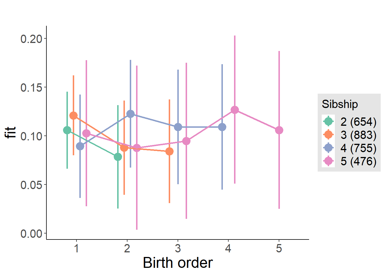
Model Comparison
###### Model 1 - Model 2
anova(m1_covariates_only, m2_birthorder_linear, m3_birthorder_nonlinear, m4_interaction)## refitting model(s) with ML (instead of REML)| Df | AIC | BIC | logLik | deviance | Chisq | Chi Df | Pr(>Chisq) |
|---|---|---|---|---|---|---|---|
| 10 | 609.6 | 668.8 | -294.8 | 589.6 | NA | NA | NA |
| 11 | 611.3 | 676.5 | -294.7 | 589.3 | 0.2297 | 1 | 0.6318 |
| 14 | 615.2 | 698.2 | -293.6 | 587.2 | 2.126 | 3 | 0.5468 |
| 20 | 620.9 | 739.4 | -290.5 | 580.9 | 6.288 | 6 | 0.3917 |
Compare birth order specifications
library(coefplot)
multiplot(outcome_naive_m1, outcome_preg_m1, outcome_uterus_m1, outcome_parental_m1, dodgeHeight = 0.6,
intercept = FALSE)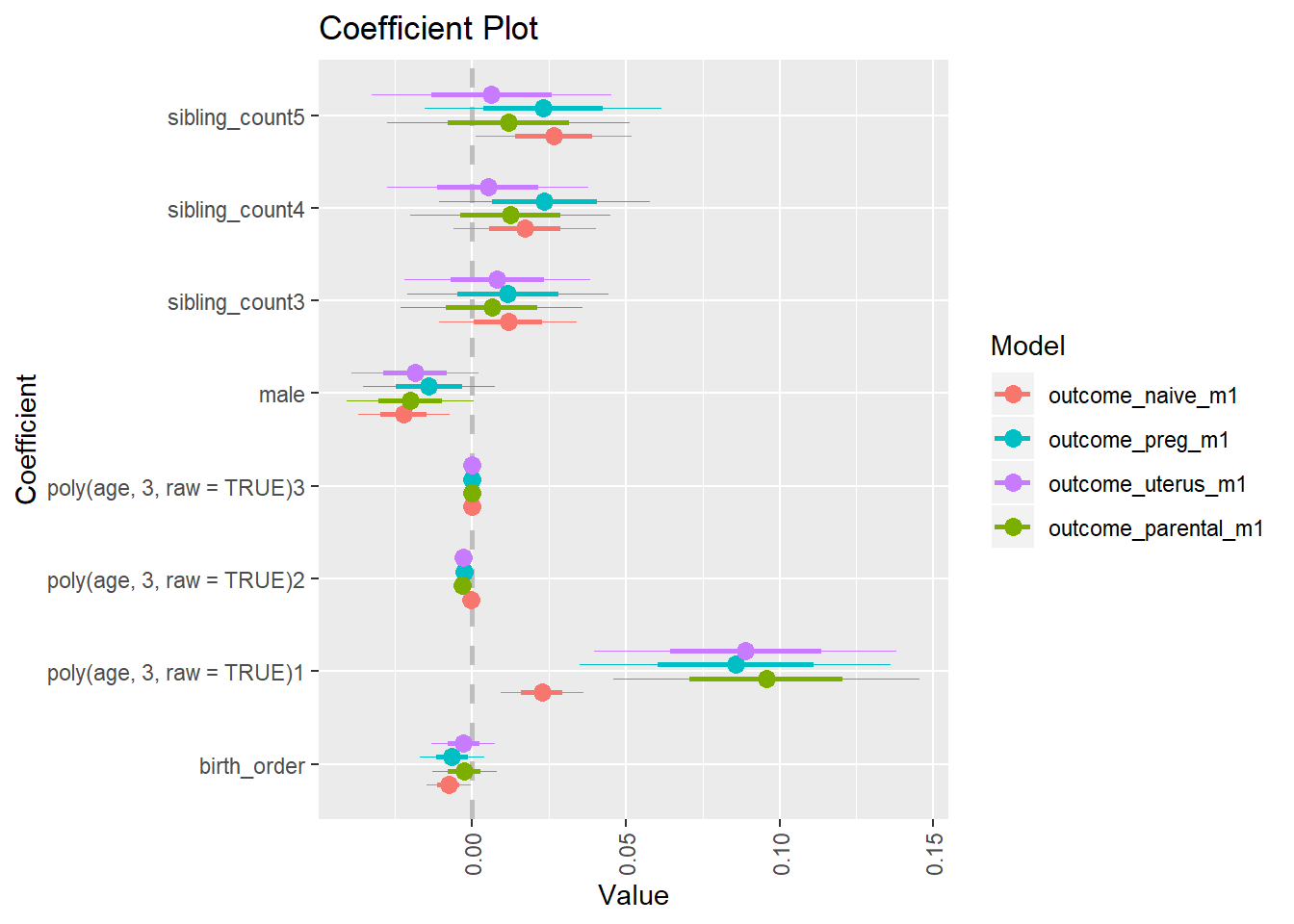
Category_Private worker
birthorder <- birthorder %>% mutate(outcome = `Category_Private worker`)
model = lmer(outcome ~ birth_order + poly(age, 3, raw = TRUE) + male + sibling_count + (1 | mother_pidlink),
data = birthorder)
compare_birthorder_specs(model)Naive birth order
outcome_naive_m1 <- update(m2_birthorder_linear, data = birthorder %>%
mutate(sibling_count = sibling_count_naive_factor,
birth_order_nonlinear = birthorder_naive_factor,
birth_order = birthorder_naive,
count_birth_order = count_birthorder_naive) %>%
filter(sibling_count != "1"))
compare_models_markdown(outcome_naive_m1)Basic Model
Model Summary
m1_covariates_only <- update(m2_birthorder_linear, formula = . ~ . - birth_order)
tidy(m1_covariates_only, conf.int = T, conf.level = 0.995)| effect | group | term | estimate | std.error | statistic | df | p.value | conf.low | conf.high |
|---|---|---|---|---|---|---|---|---|---|
| fixed | NA | (Intercept) | -0.1396 | 0.1387 | -1.006 | 4529 | 0.3144 | -0.5289 | 0.2498 |
| fixed | NA | poly(age, 3, raw = TRUE)1 | 0.06859 | 0.01239 | 5.535 | 4443 | 0.0000000329 | 0.03381 | 0.1034 |
| fixed | NA | poly(age, 3, raw = TRUE)2 | -0.002108 | 0.0003447 | -6.114 | 4331 | 0.000000001055 | -0.003075 | -0.00114 |
| fixed | NA | poly(age, 3, raw = TRUE)3 | 0.00001739 | 0.000003019 | 5.759 | 4227 | 0.000000009061 | 0.000008912 | 0.00002586 |
| fixed | NA | male | 0.02924 | 0.01385 | 2.111 | 4661 | 0.03484 | -0.009644 | 0.06812 |
| fixed | NA | sibling_count3 | -0.0009719 | 0.0206 | -0.04719 | 3351 | 0.9624 | -0.05878 | 0.05684 |
| fixed | NA | sibling_count4 | -0.01074 | 0.02087 | -0.5144 | 3179 | 0.607 | -0.06933 | 0.04786 |
| fixed | NA | sibling_count5 | -0.03073 | 0.02184 | -1.407 | 2983 | 0.1596 | -0.09204 | 0.03058 |
| ran_pars | mother_pidlink | sd__(Intercept) | 0.2186 | NA | NA | NA | NA | NA | NA |
| ran_pars | Residual | sd__Observation | 0.4315 | NA | NA | NA | NA | NA | NA |
Coefficient Plot
plot(allEffects(m1_covariates_only, confidence.level = 0.995))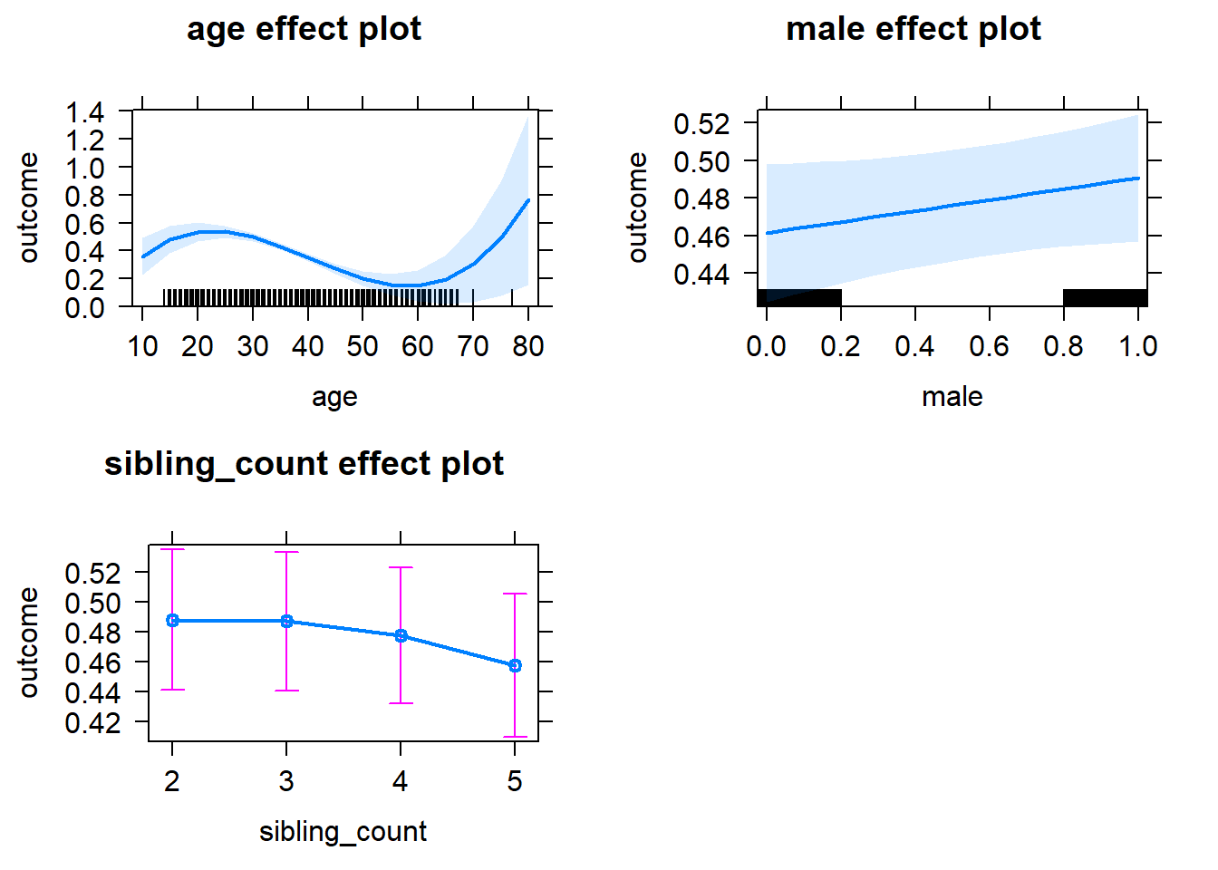
Add Birth Order Linear
Model Summary
tidy(m2_birthorder_linear, conf.int = T, conf.level = 0.995)| effect | group | term | estimate | std.error | statistic | df | p.value | conf.low | conf.high |
|---|---|---|---|---|---|---|---|---|---|
| fixed | NA | (Intercept) | -0.1421 | 0.1387 | -1.025 | 4531 | 0.3055 | -0.5313 | 0.2471 |
| fixed | NA | birth_order | -0.01581 | 0.006719 | -2.353 | 4027 | 0.01868 | -0.03467 | 0.003052 |
| fixed | NA | poly(age, 3, raw = TRUE)1 | 0.071 | 0.01243 | 5.712 | 4446 | 0.00000001189 | 0.03611 | 0.1059 |
| fixed | NA | poly(age, 3, raw = TRUE)2 | -0.00217 | 0.0003456 | -6.279 | 4325 | 0.0000000003745 | -0.00314 | -0.0012 |
| fixed | NA | poly(age, 3, raw = TRUE)3 | 0.00001781 | 0.000003024 | 5.892 | 4221 | 0.000000004117 | 0.000009327 | 0.0000263 |
| fixed | NA | male | 0.02909 | 0.01384 | 2.101 | 4659 | 0.03568 | -0.009772 | 0.06795 |
| fixed | NA | sibling_count3 | 0.004861 | 0.02074 | 0.2344 | 3439 | 0.8147 | -0.05336 | 0.06308 |
| fixed | NA | sibling_count4 | 0.001696 | 0.02153 | 0.07879 | 3521 | 0.9372 | -0.05873 | 0.06213 |
| fixed | NA | sibling_count5 | -0.01073 | 0.02343 | -0.4579 | 3667 | 0.6471 | -0.07651 | 0.05505 |
| ran_pars | mother_pidlink | sd__(Intercept) | 0.219 | NA | NA | NA | NA | NA | NA |
| ran_pars | Residual | sd__Observation | 0.431 | NA | NA | NA | NA | NA | NA |
Coefficient Plot
plot_birthorder2(m2_birthorder_linear, separate = FALSE)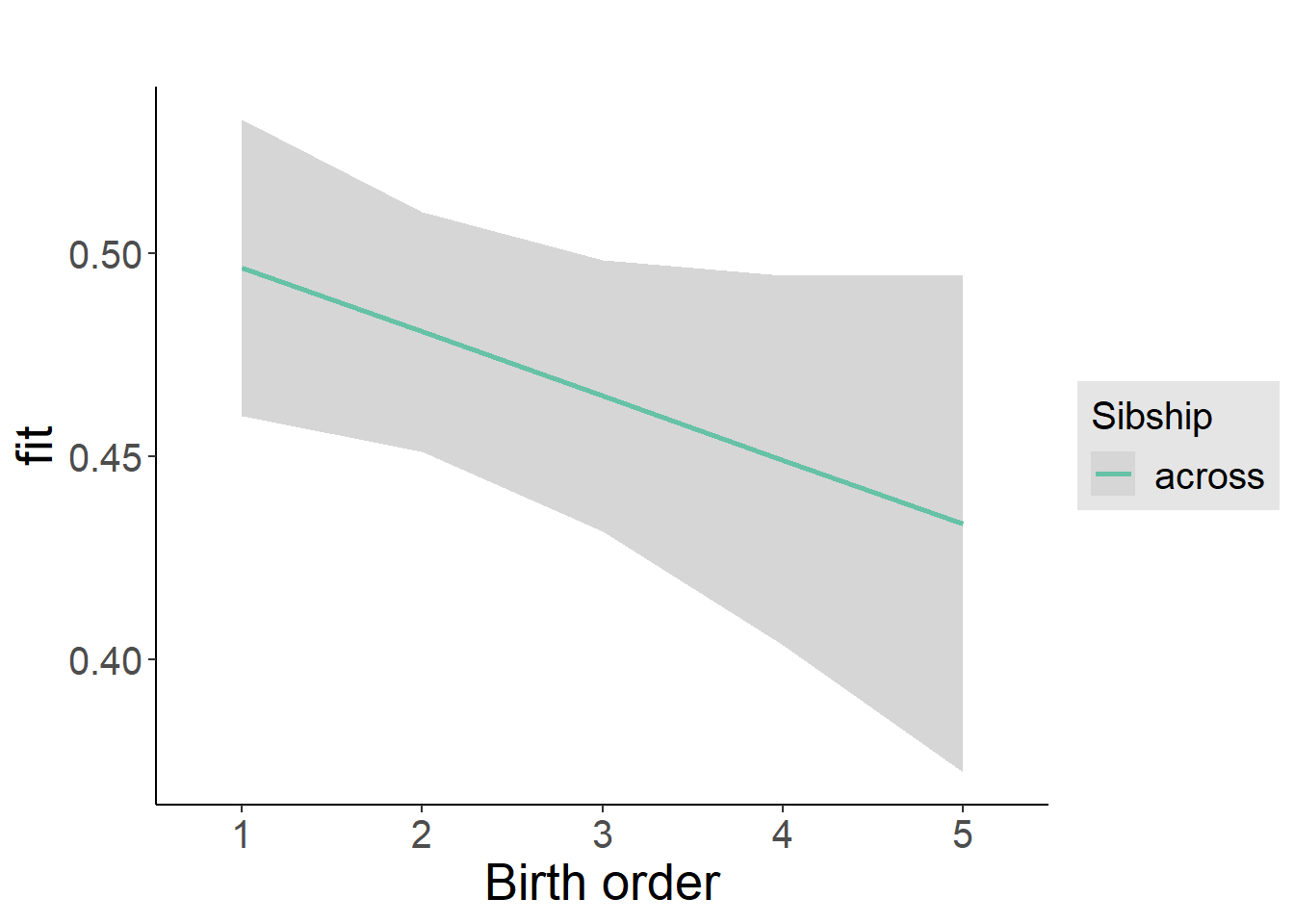
Add Birth Order Factor
Model Summary
m3_birthorder_nonlinear = update(m1_covariates_only, formula = . ~ . + birth_order_nonlinear)
tidy(m3_birthorder_nonlinear, conf.int = T, conf.level = 0.995)| effect | group | term | estimate | std.error | statistic | df | p.value | conf.low | conf.high |
|---|---|---|---|---|---|---|---|---|---|
| fixed | NA | (Intercept) | -0.1492 | 0.139 | -1.073 | 4534 | 0.2833 | -0.5394 | 0.2411 |
| fixed | NA | poly(age, 3, raw = TRUE)1 | 0.07071 | 0.01243 | 5.688 | 4440 | 0.00000001369 | 0.03582 | 0.1056 |
| fixed | NA | poly(age, 3, raw = TRUE)2 | -0.002151 | 0.0003458 | -6.221 | 4314 | 0.0000000005401 | -0.003122 | -0.001181 |
| fixed | NA | poly(age, 3, raw = TRUE)3 | 0.00001755 | 0.000003026 | 5.8 | 4202 | 0.000000007104 | 0.000009059 | 0.00002605 |
| fixed | NA | male | 0.02952 | 0.01385 | 2.132 | 4657 | 0.03307 | -0.009349 | 0.06839 |
| fixed | NA | sibling_count3 | 0.007167 | 0.02105 | 0.3405 | 3587 | 0.7335 | -0.05191 | 0.06625 |
| fixed | NA | sibling_count4 | 0.00145 | 0.02185 | 0.06637 | 3674 | 0.9471 | -0.05989 | 0.06279 |
| fixed | NA | sibling_count5 | -0.01578 | 0.02362 | -0.6681 | 3759 | 0.5041 | -0.08209 | 0.05053 |
| fixed | NA | birth_order_nonlinear2 | -0.04204 | 0.01619 | -2.597 | 3977 | 0.009434 | -0.08748 | 0.003397 |
| fixed | NA | birth_order_nonlinear3 | -0.04759 | 0.02057 | -2.314 | 3855 | 0.02073 | -0.1053 | 0.01014 |
| fixed | NA | birth_order_nonlinear4 | -0.04298 | 0.02669 | -1.61 | 3775 | 0.1074 | -0.1179 | 0.03193 |
| fixed | NA | birth_order_nonlinear5 | -0.04299 | 0.03855 | -1.115 | 3759 | 0.2649 | -0.1512 | 0.06523 |
| ran_pars | mother_pidlink | sd__(Intercept) | 0.2186 | NA | NA | NA | NA | NA | NA |
| ran_pars | Residual | sd__Observation | 0.4312 | NA | NA | NA | NA | NA | NA |
Coefficient Plot
plot_birthorder(m3_birthorder_nonlinear, separate = FALSE)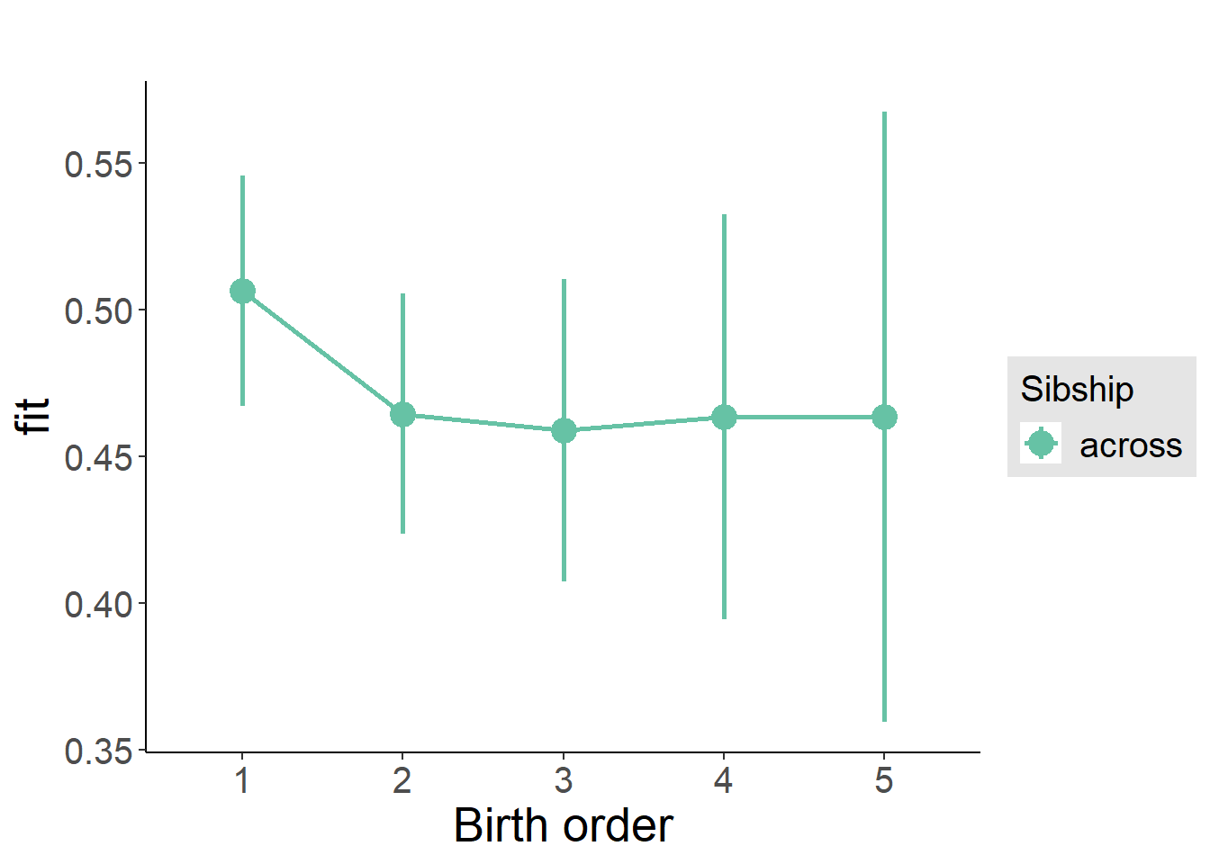
Add Interaction
Model Summary
m4_interaction = update(m3_birthorder_nonlinear, formula = . ~ . - birth_order_nonlinear - sibling_count + count_birth_order)
tidy(m4_interaction, conf.int = T, conf.level = 0.995)| effect | group | term | estimate | std.error | statistic | df | p.value | conf.low | conf.high |
|---|---|---|---|---|---|---|---|---|---|
| fixed | NA | (Intercept) | -0.1495 | 0.1393 | -1.073 | 4537 | 0.2831 | -0.5404 | 0.2414 |
| fixed | NA | poly(age, 3, raw = TRUE)1 | 0.07115 | 0.01245 | 5.717 | 4436 | 0.00000001156 | 0.03622 | 0.1061 |
| fixed | NA | poly(age, 3, raw = TRUE)2 | -0.00216 | 0.0003461 | -6.241 | 4310 | 0.0000000004766 | -0.003131 | -0.001188 |
| fixed | NA | poly(age, 3, raw = TRUE)3 | 0.00001759 | 0.000003028 | 5.81 | 4197 | 0.000000006713 | 0.000009094 | 0.00002609 |
| fixed | NA | male | 0.02963 | 0.01386 | 2.138 | 4649 | 0.03259 | -0.009276 | 0.06853 |
| fixed | NA | count_birth_order2/2 | -0.05761 | 0.0275 | -2.095 | 3974 | 0.03625 | -0.1348 | 0.01959 |
| fixed | NA | count_birth_order1/3 | -0.0008044 | 0.02708 | -0.0297 | 4777 | 0.9763 | -0.07683 | 0.07522 |
| fixed | NA | count_birth_order2/3 | -0.03296 | 0.03 | -1.099 | 4802 | 0.2719 | -0.1172 | 0.05124 |
| fixed | NA | count_birth_order3/3 | -0.0523 | 0.03296 | -1.587 | 4804 | 0.1127 | -0.1448 | 0.04023 |
| fixed | NA | count_birth_order1/4 | -0.006749 | 0.02965 | -0.2276 | 4802 | 0.82 | -0.08998 | 0.07648 |
| fixed | NA | count_birth_order2/4 | -0.04075 | 0.03178 | -1.282 | 4806 | 0.1998 | -0.1299 | 0.04845 |
| fixed | NA | count_birth_order3/4 | -0.04033 | 0.03387 | -1.191 | 4799 | 0.2338 | -0.1354 | 0.05474 |
| fixed | NA | count_birth_order4/4 | -0.06524 | 0.03602 | -1.811 | 4792 | 0.07015 | -0.1663 | 0.03586 |
| fixed | NA | count_birth_order1/5 | -0.02917 | 0.03361 | -0.8679 | 4803 | 0.3855 | -0.1235 | 0.06517 |
| fixed | NA | count_birth_order2/5 | -0.06593 | 0.03565 | -1.849 | 4794 | 0.06448 | -0.166 | 0.03415 |
| fixed | NA | count_birth_order3/5 | -0.07601 | 0.03751 | -2.027 | 4778 | 0.04274 | -0.1813 | 0.02926 |
| fixed | NA | count_birth_order4/5 | -0.04191 | 0.03939 | -1.064 | 4729 | 0.2874 | -0.1525 | 0.06866 |
| fixed | NA | count_birth_order5/5 | -0.06442 | 0.03945 | -1.633 | 4762 | 0.1026 | -0.1752 | 0.04633 |
| ran_pars | mother_pidlink | sd__(Intercept) | 0.2187 | NA | NA | NA | NA | NA | NA |
| ran_pars | Residual | sd__Observation | 0.4314 | NA | NA | NA | NA | NA | NA |
Coefficient Plot
plot_birthorder(m4_interaction)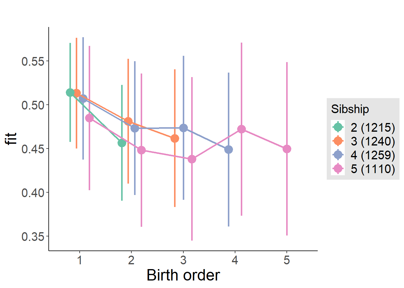
Model Comparison
###### Model 1 - Model 2
anova(m1_covariates_only, m2_birthorder_linear, m3_birthorder_nonlinear, m4_interaction)## refitting model(s) with ML (instead of REML)| Df | AIC | BIC | logLik | deviance | Chisq | Chi Df | Pr(>Chisq) |
|---|---|---|---|---|---|---|---|
| 10 | 6616 | 6680 | -3298 | 6596 | NA | NA | NA |
| 11 | 6612 | 6683 | -3295 | 6590 | 5.536 | 1 | 0.01863 |
| 14 | 6614 | 6705 | -3293 | 6586 | 3.852 | 3 | 0.2778 |
| 20 | 6624 | 6754 | -3292 | 6584 | 1.688 | 6 | 0.946 |
Maternal birth order
outcome_uterus_m1 <- update(m2_birthorder_linear, data = birthorder %>%
mutate(sibling_count = sibling_count_uterus_alive_factor,
birth_order_nonlinear = birthorder_uterus_alive_factor,
birth_order = birthorder_uterus_alive,
count_birth_order = count_birthorder_uterus_alive) %>%
filter(sibling_count != "1"))
compare_models_markdown(outcome_uterus_m1)Basic Model
Model Summary
m1_covariates_only <- update(m2_birthorder_linear, formula = . ~ . - birth_order)
tidy(m1_covariates_only, conf.int = T, conf.level = 0.995)| effect | group | term | estimate | std.error | statistic | df | p.value | conf.low | conf.high |
|---|---|---|---|---|---|---|---|---|---|
| fixed | NA | (Intercept) | -2.628 | 0.4004 | -6.562 | 2760 | 0.00000000006304 | -3.751 | -1.504 |
| fixed | NA | poly(age, 3, raw = TRUE)1 | 0.3389 | 0.04435 | 7.642 | 2760 | 2.937e-14 | 0.2144 | 0.4634 |
| fixed | NA | poly(age, 3, raw = TRUE)2 | -0.01116 | 0.001573 | -7.098 | 2760 | 1.601e-12 | -0.01558 | -0.006749 |
| fixed | NA | poly(age, 3, raw = TRUE)3 | 0.0001141 | 0.00001787 | 6.386 | 2760 | 0.0000000001988 | 0.00006394 | 0.0001642 |
| fixed | NA | male | 0.02993 | 0.01869 | 1.601 | 2705 | 0.1094 | -0.02253 | 0.08239 |
| fixed | NA | sibling_count3 | -0.03668 | 0.02673 | -1.372 | 2184 | 0.1701 | -0.1117 | 0.03835 |
| fixed | NA | sibling_count4 | -0.03183 | 0.0278 | -1.145 | 2052 | 0.2523 | -0.1098 | 0.0462 |
| fixed | NA | sibling_count5 | -0.06908 | 0.03104 | -2.226 | 1851 | 0.02615 | -0.1562 | 0.01804 |
| ran_pars | mother_pidlink | sd__(Intercept) | 0.2124 | NA | NA | NA | NA | NA | NA |
| ran_pars | Residual | sd__Observation | 0.441 | NA | NA | NA | NA | NA | NA |
Coefficient Plot
plot(allEffects(m1_covariates_only, confidence.level = 0.995))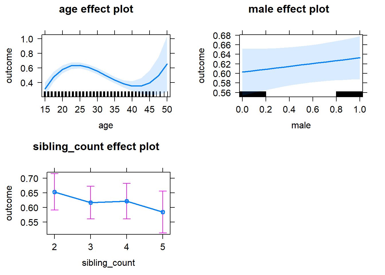
Add Birth Order Linear
Model Summary
tidy(m2_birthorder_linear, conf.int = T, conf.level = 0.995)| effect | group | term | estimate | std.error | statistic | df | p.value | conf.low | conf.high |
|---|---|---|---|---|---|---|---|---|---|
| fixed | NA | (Intercept) | -2.625 | 0.4004 | -6.555 | 2759 | 0.0000000000662 | -3.749 | -1.501 |
| fixed | NA | birth_order | -0.006695 | 0.009355 | -0.7157 | 2563 | 0.4743 | -0.03296 | 0.01957 |
| fixed | NA | poly(age, 3, raw = TRUE)1 | 0.3394 | 0.04436 | 7.652 | 2759 | 2.72e-14 | 0.2149 | 0.464 |
| fixed | NA | poly(age, 3, raw = TRUE)2 | -0.01117 | 0.001573 | -7.102 | 2759 | 1.557e-12 | -0.01559 | -0.006756 |
| fixed | NA | poly(age, 3, raw = TRUE)3 | 0.000114 | 0.00001787 | 6.38 | 2759 | 0.0000000002071 | 0.00006384 | 0.0001641 |
| fixed | NA | male | 0.02993 | 0.01869 | 1.601 | 2704 | 0.1095 | -0.02254 | 0.08239 |
| fixed | NA | sibling_count3 | -0.03342 | 0.02711 | -1.233 | 2216 | 0.2179 | -0.1095 | 0.04269 |
| fixed | NA | sibling_count4 | -0.02488 | 0.02944 | -0.8451 | 2169 | 0.3982 | -0.1075 | 0.05776 |
| fixed | NA | sibling_count5 | -0.05743 | 0.03505 | -1.639 | 2153 | 0.1014 | -0.1558 | 0.04094 |
| ran_pars | mother_pidlink | sd__(Intercept) | 0.2122 | NA | NA | NA | NA | NA | NA |
| ran_pars | Residual | sd__Observation | 0.4411 | NA | NA | NA | NA | NA | NA |
Coefficient Plot
plot_birthorder2(m2_birthorder_linear, separate = FALSE)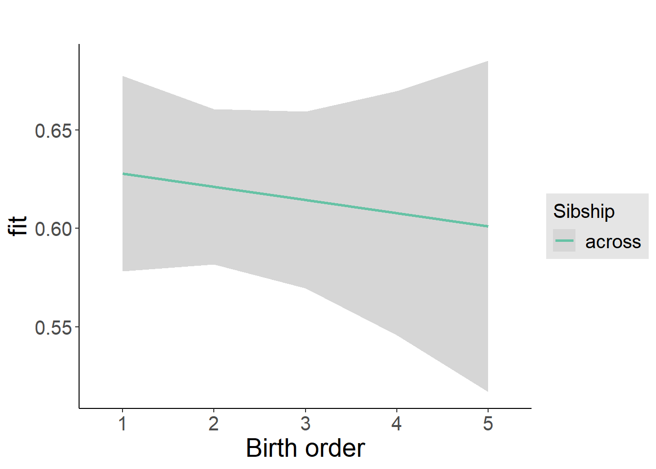
Add Birth Order Factor
Model Summary
m3_birthorder_nonlinear = update(m1_covariates_only, formula = . ~ . + birth_order_nonlinear)
tidy(m3_birthorder_nonlinear, conf.int = T, conf.level = 0.995)| effect | group | term | estimate | std.error | statistic | df | p.value | conf.low | conf.high |
|---|---|---|---|---|---|---|---|---|---|
| fixed | NA | (Intercept) | -2.648 | 0.4013 | -6.599 | 2756 | 0.00000000004948 | -3.774 | -1.522 |
| fixed | NA | poly(age, 3, raw = TRUE)1 | 0.3415 | 0.04444 | 7.685 | 2756 | 2.119e-14 | 0.2167 | 0.4662 |
| fixed | NA | poly(age, 3, raw = TRUE)2 | -0.01124 | 0.001576 | -7.133 | 2756 | 1.25e-12 | -0.01566 | -0.006816 |
| fixed | NA | poly(age, 3, raw = TRUE)3 | 0.0001147 | 0.00001789 | 6.409 | 2756 | 0.000000000172 | 0.00006445 | 0.0001649 |
| fixed | NA | male | 0.03068 | 0.0187 | 1.64 | 2702 | 0.1011 | -0.02182 | 0.08317 |
| fixed | NA | sibling_count3 | -0.0364 | 0.02749 | -1.324 | 2275 | 0.1856 | -0.1136 | 0.04077 |
| fixed | NA | sibling_count4 | -0.02095 | 0.02979 | -0.7031 | 2224 | 0.4821 | -0.1046 | 0.06269 |
| fixed | NA | sibling_count5 | -0.06187 | 0.03546 | -1.745 | 2196 | 0.08118 | -0.1614 | 0.03767 |
| fixed | NA | birth_order_nonlinear2 | -0.01621 | 0.02221 | -0.7302 | 2292 | 0.4654 | -0.07855 | 0.04612 |
| fixed | NA | birth_order_nonlinear3 | -0.001198 | 0.02715 | -0.04413 | 2352 | 0.9648 | -0.07741 | 0.07502 |
| fixed | NA | birth_order_nonlinear4 | -0.05709 | 0.03612 | -1.581 | 2415 | 0.1141 | -0.1585 | 0.0443 |
| fixed | NA | birth_order_nonlinear5 | 0.01887 | 0.0554 | 0.3407 | 2336 | 0.7334 | -0.1366 | 0.1744 |
| ran_pars | mother_pidlink | sd__(Intercept) | 0.2125 | NA | NA | NA | NA | NA | NA |
| ran_pars | Residual | sd__Observation | 0.441 | NA | NA | NA | NA | NA | NA |
Coefficient Plot
plot_birthorder(m3_birthorder_nonlinear, separate = FALSE)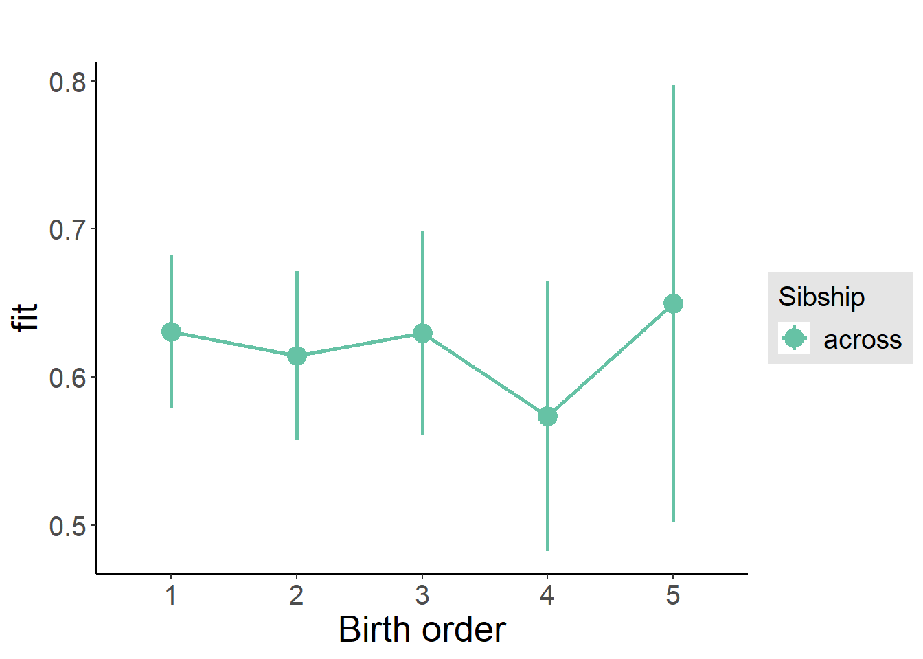
Add Interaction
Model Summary
m4_interaction = update(m3_birthorder_nonlinear, formula = . ~ . - birth_order_nonlinear - sibling_count + count_birth_order)
tidy(m4_interaction, conf.int = T, conf.level = 0.995)| effect | group | term | estimate | std.error | statistic | df | p.value | conf.low | conf.high |
|---|---|---|---|---|---|---|---|---|---|
| fixed | NA | (Intercept) | -2.655 | 0.4019 | -6.607 | 2750 | 0.00000000004703 | -3.783 | -1.527 |
| fixed | NA | poly(age, 3, raw = TRUE)1 | 0.3416 | 0.0445 | 7.678 | 2750 | 2.228e-14 | 0.2167 | 0.4665 |
| fixed | NA | poly(age, 3, raw = TRUE)2 | -0.01125 | 0.001578 | -7.128 | 2750 | 1.3e-12 | -0.01568 | -0.006818 |
| fixed | NA | poly(age, 3, raw = TRUE)3 | 0.0001148 | 0.00001792 | 6.405 | 2750 | 0.0000000001761 | 0.00006449 | 0.0001651 |
| fixed | NA | male | 0.03024 | 0.01874 | 1.614 | 2695 | 0.1067 | -0.02236 | 0.08284 |
| fixed | NA | count_birth_order2/2 | 0.002125 | 0.04039 | 0.05263 | 2375 | 0.958 | -0.1112 | 0.1155 |
| fixed | NA | count_birth_order1/3 | -0.02675 | 0.03462 | -0.7728 | 2743 | 0.4397 | -0.1239 | 0.07042 |
| fixed | NA | count_birth_order2/3 | -0.04489 | 0.03839 | -1.169 | 2750 | 0.2424 | -0.1526 | 0.06287 |
| fixed | NA | count_birth_order3/3 | -0.04155 | 0.04149 | -1.001 | 2745 | 0.3168 | -0.158 | 0.07493 |
| fixed | NA | count_birth_order1/4 | -0.007495 | 0.03985 | -0.1881 | 2749 | 0.8508 | -0.1194 | 0.1044 |
| fixed | NA | count_birth_order2/4 | -0.031 | 0.0418 | -0.7416 | 2746 | 0.4584 | -0.1483 | 0.08634 |
| fixed | NA | count_birth_order3/4 | -0.02146 | 0.04378 | -0.4902 | 2733 | 0.624 | -0.1443 | 0.1014 |
| fixed | NA | count_birth_order4/4 | -0.07964 | 0.04638 | -1.717 | 2729 | 0.08605 | -0.2098 | 0.05054 |
| fixed | NA | count_birth_order1/5 | -0.06377 | 0.05233 | -1.219 | 2746 | 0.2231 | -0.2107 | 0.08312 |
| fixed | NA | count_birth_order2/5 | -0.1064 | 0.0567 | -1.877 | 2707 | 0.06061 | -0.2656 | 0.05273 |
| fixed | NA | count_birth_order3/5 | -0.03041 | 0.05308 | -0.5729 | 2715 | 0.5667 | -0.1794 | 0.1186 |
| fixed | NA | count_birth_order4/5 | -0.1034 | 0.05156 | -2.006 | 2712 | 0.04498 | -0.2482 | 0.04132 |
| fixed | NA | count_birth_order5/5 | -0.03676 | 0.05404 | -0.6803 | 2704 | 0.4964 | -0.1884 | 0.1149 |
| ran_pars | mother_pidlink | sd__(Intercept) | 0.2127 | NA | NA | NA | NA | NA | NA |
| ran_pars | Residual | sd__Observation | 0.4413 | NA | NA | NA | NA | NA | NA |
Coefficient Plot
plot_birthorder(m4_interaction)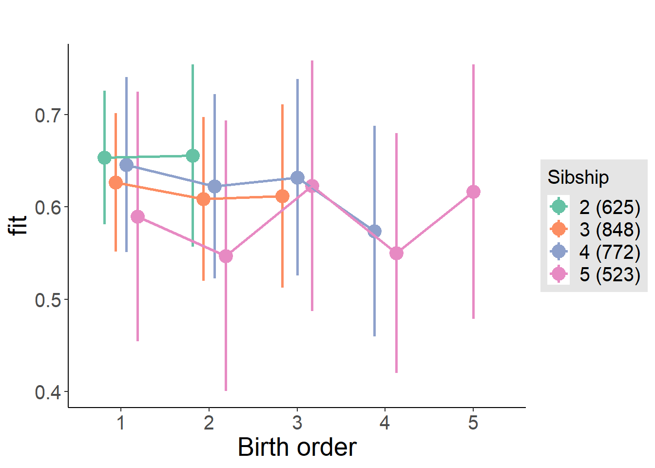
Model Comparison
###### Model 1 - Model 2
anova(m1_covariates_only, m2_birthorder_linear, m3_birthorder_nonlinear, m4_interaction)## refitting model(s) with ML (instead of REML)| Df | AIC | BIC | logLik | deviance | Chisq | Chi Df | Pr(>Chisq) |
|---|---|---|---|---|---|---|---|
| 10 | 3881 | 3941 | -1931 | 3861 | NA | NA | NA |
| 11 | 3883 | 3948 | -1930 | 3861 | 0.5141 | 1 | 0.4734 |
| 14 | 3886 | 3969 | -1929 | 3858 | 3.018 | 3 | 0.3888 |
| 20 | 3896 | 4015 | -1928 | 3856 | 1.348 | 6 | 0.9689 |
Maternal pregnancy order
outcome_preg_m1 <- update(m2_birthorder_linear, data = birthorder %>%
mutate(sibling_count = sibling_count_uterus_preg_factor,
birth_order_nonlinear = birthorder_uterus_preg_factor,
birth_order = birthorder_uterus_preg,
count_birth_order = count_birthorder_uterus_preg
) %>%
filter(sibling_count != "1"))
compare_models_markdown(outcome_preg_m1)Basic Model
Model Summary
m1_covariates_only <- update(m2_birthorder_linear, formula = . ~ . - birth_order)
tidy(m1_covariates_only, conf.int = T, conf.level = 0.995)| effect | group | term | estimate | std.error | statistic | df | p.value | conf.low | conf.high |
|---|---|---|---|---|---|---|---|---|---|
| fixed | NA | (Intercept) | -2.616 | 0.4144 | -6.314 | 2531 | 0.0000000003194 | -3.78 | -1.453 |
| fixed | NA | poly(age, 3, raw = TRUE)1 | 0.3375 | 0.04592 | 7.35 | 2530 | 2.663e-13 | 0.2086 | 0.4665 |
| fixed | NA | poly(age, 3, raw = TRUE)2 | -0.01112 | 0.001629 | -6.83 | 2530 | 0.00000000001056 | -0.0157 | -0.006552 |
| fixed | NA | poly(age, 3, raw = TRUE)3 | 0.0001134 | 0.0000185 | 6.132 | 2530 | 0.000000001003 | 0.00006152 | 0.0001654 |
| fixed | NA | male | 0.02442 | 0.0195 | 1.252 | 2476 | 0.2106 | -0.03032 | 0.07916 |
| fixed | NA | sibling_count3 | -0.01048 | 0.02931 | -0.3575 | 2043 | 0.7207 | -0.09276 | 0.0718 |
| fixed | NA | sibling_count4 | -0.01521 | 0.02973 | -0.5116 | 1964 | 0.609 | -0.09866 | 0.06824 |
| fixed | NA | sibling_count5 | -0.04316 | 0.03146 | -1.372 | 1840 | 0.1703 | -0.1315 | 0.04516 |
| ran_pars | mother_pidlink | sd__(Intercept) | 0.2183 | NA | NA | NA | NA | NA | NA |
| ran_pars | Residual | sd__Observation | 0.4379 | NA | NA | NA | NA | NA | NA |
Coefficient Plot
plot(allEffects(m1_covariates_only, confidence.level = 0.995))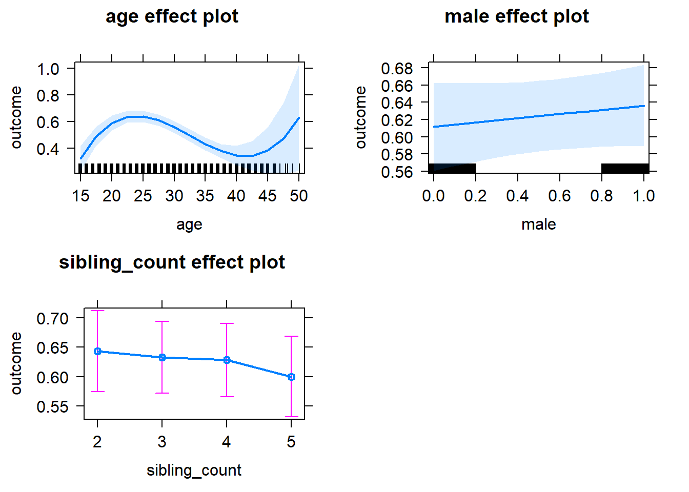
Add Birth Order Linear
Model Summary
tidy(m2_birthorder_linear, conf.int = T, conf.level = 0.995)| effect | group | term | estimate | std.error | statistic | df | p.value | conf.low | conf.high |
|---|---|---|---|---|---|---|---|---|---|
| fixed | NA | (Intercept) | -2.613 | 0.4145 | -6.303 | 2530 | 0.000000000344 | -3.776 | -1.449 |
| fixed | NA | birth_order | -0.004532 | 0.00948 | -0.478 | 2393 | 0.6327 | -0.03114 | 0.02208 |
| fixed | NA | poly(age, 3, raw = TRUE)1 | 0.3377 | 0.04593 | 7.353 | 2530 | 2.612e-13 | 0.2088 | 0.4667 |
| fixed | NA | poly(age, 3, raw = TRUE)2 | -0.01113 | 0.001629 | -6.83 | 2529 | 0.00000000001059 | -0.0157 | -0.006553 |
| fixed | NA | poly(age, 3, raw = TRUE)3 | 0.0001134 | 0.0000185 | 6.126 | 2529 | 0.000000001044 | 0.00006141 | 0.0001653 |
| fixed | NA | male | 0.02429 | 0.01951 | 1.245 | 2475 | 0.2131 | -0.03046 | 0.07905 |
| fixed | NA | sibling_count3 | -0.008213 | 0.0297 | -0.2765 | 2061 | 0.7822 | -0.09158 | 0.07515 |
| fixed | NA | sibling_count4 | -0.0108 | 0.03113 | -0.3468 | 2034 | 0.7288 | -0.09819 | 0.0766 |
| fixed | NA | sibling_count5 | -0.03579 | 0.03504 | -1.021 | 2047 | 0.3072 | -0.1342 | 0.06257 |
| ran_pars | mother_pidlink | sd__(Intercept) | 0.2183 | NA | NA | NA | NA | NA | NA |
| ran_pars | Residual | sd__Observation | 0.438 | NA | NA | NA | NA | NA | NA |
Coefficient Plot
plot_birthorder2(m2_birthorder_linear, separate = FALSE)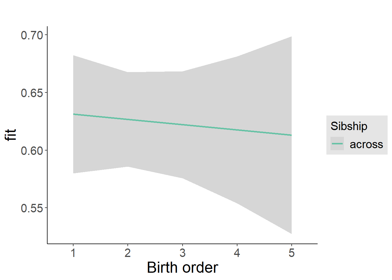
Add Birth Order Factor
Model Summary
m3_birthorder_nonlinear = update(m1_covariates_only, formula = . ~ . + birth_order_nonlinear)
tidy(m3_birthorder_nonlinear, conf.int = T, conf.level = 0.995)| effect | group | term | estimate | std.error | statistic | df | p.value | conf.low | conf.high |
|---|---|---|---|---|---|---|---|---|---|
| fixed | NA | (Intercept) | -2.61 | 0.4154 | -6.284 | 2527 | 0.0000000003879 | -3.777 | -1.444 |
| fixed | NA | poly(age, 3, raw = TRUE)1 | 0.3377 | 0.04603 | 7.337 | 2527 | 2.928e-13 | 0.2085 | 0.4669 |
| fixed | NA | poly(age, 3, raw = TRUE)2 | -0.01112 | 0.001632 | -6.815 | 2527 | 0.00000000001176 | -0.0157 | -0.006541 |
| fixed | NA | poly(age, 3, raw = TRUE)3 | 0.0001133 | 0.00001854 | 6.111 | 2527 | 0.000000001142 | 0.00006125 | 0.0001653 |
| fixed | NA | male | 0.02479 | 0.01951 | 1.271 | 2471 | 0.2039 | -0.02997 | 0.07954 |
| fixed | NA | sibling_count3 | -0.009925 | 0.0301 | -0.3298 | 2107 | 0.7416 | -0.09441 | 0.07456 |
| fixed | NA | sibling_count4 | -0.005475 | 0.03149 | -0.1739 | 2076 | 0.862 | -0.09386 | 0.08291 |
| fixed | NA | sibling_count5 | -0.04175 | 0.03524 | -1.185 | 2067 | 0.2363 | -0.1407 | 0.05718 |
| fixed | NA | birth_order_nonlinear2 | -0.0257 | 0.02302 | -1.117 | 2110 | 0.2643 | -0.09031 | 0.03891 |
| fixed | NA | birth_order_nonlinear3 | -0.002134 | 0.02845 | -0.07502 | 2195 | 0.9402 | -0.08198 | 0.07772 |
| fixed | NA | birth_order_nonlinear4 | -0.05797 | 0.03734 | -1.553 | 2240 | 0.1206 | -0.1628 | 0.04683 |
| fixed | NA | birth_order_nonlinear5 | 0.03924 | 0.05328 | 0.7364 | 2162 | 0.4616 | -0.1103 | 0.1888 |
| ran_pars | mother_pidlink | sd__(Intercept) | 0.2197 | NA | NA | NA | NA | NA | NA |
| ran_pars | Residual | sd__Observation | 0.4372 | NA | NA | NA | NA | NA | NA |
Coefficient Plot
plot_birthorder(m3_birthorder_nonlinear, separate = FALSE)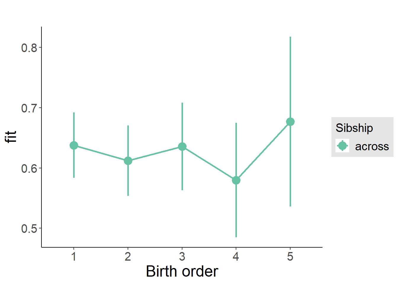
Add Interaction
Model Summary
m4_interaction = update(m3_birthorder_nonlinear, formula = . ~ . - birth_order_nonlinear - sibling_count + count_birth_order)
tidy(m4_interaction, conf.int = T, conf.level = 0.995)| effect | group | term | estimate | std.error | statistic | df | p.value | conf.low | conf.high |
|---|---|---|---|---|---|---|---|---|---|
| fixed | NA | (Intercept) | -2.595 | 0.4162 | -6.235 | 2521 | 0.0000000005284 | -3.763 | -1.427 |
| fixed | NA | poly(age, 3, raw = TRUE)1 | 0.337 | 0.04611 | 7.31 | 2521 | 3.576e-13 | 0.2076 | 0.4664 |
| fixed | NA | poly(age, 3, raw = TRUE)2 | -0.0111 | 0.001635 | -6.789 | 2521 | 0.000000000014 | -0.01569 | -0.006511 |
| fixed | NA | poly(age, 3, raw = TRUE)3 | 0.0001131 | 0.00001857 | 6.089 | 2521 | 0.000000001312 | 0.00006095 | 0.0001652 |
| fixed | NA | male | 0.02467 | 0.01957 | 1.261 | 2466 | 0.2076 | -0.03026 | 0.07959 |
| fixed | NA | count_birth_order2/2 | -0.05466 | 0.0444 | -1.231 | 2242 | 0.2185 | -0.1793 | 0.06999 |
| fixed | NA | count_birth_order1/3 | -0.01649 | 0.03825 | -0.4311 | 2515 | 0.6665 | -0.1238 | 0.09087 |
| fixed | NA | count_birth_order2/3 | -0.04109 | 0.04152 | -0.9899 | 2521 | 0.3223 | -0.1576 | 0.07544 |
| fixed | NA | count_birth_order3/3 | -0.03243 | 0.0456 | -0.7113 | 2515 | 0.477 | -0.1604 | 0.09556 |
| fixed | NA | count_birth_order1/4 | -0.03994 | 0.0417 | -0.958 | 2519 | 0.3382 | -0.157 | 0.0771 |
| fixed | NA | count_birth_order2/4 | -0.02837 | 0.0434 | -0.6536 | 2520 | 0.5134 | -0.1502 | 0.09347 |
| fixed | NA | count_birth_order3/4 | -0.007489 | 0.04734 | -0.1582 | 2503 | 0.8743 | -0.1404 | 0.1254 |
| fixed | NA | count_birth_order4/4 | -0.05599 | 0.05045 | -1.11 | 2497 | 0.2673 | -0.1976 | 0.08564 |
| fixed | NA | count_birth_order1/5 | -0.03856 | 0.05 | -0.7712 | 2520 | 0.4407 | -0.1789 | 0.1018 |
| fixed | NA | count_birth_order2/5 | -0.0787 | 0.0518 | -1.519 | 2507 | 0.1288 | -0.2241 | 0.0667 |
| fixed | NA | count_birth_order3/5 | -0.04973 | 0.05261 | -0.9452 | 2491 | 0.3446 | -0.1974 | 0.09796 |
| fixed | NA | count_birth_order4/5 | -0.1275 | 0.05336 | -2.389 | 2476 | 0.01695 | -0.2773 | 0.02229 |
| fixed | NA | count_birth_order5/5 | -0.01228 | 0.05374 | -0.2284 | 2476 | 0.8193 | -0.1631 | 0.1386 |
| ran_pars | mother_pidlink | sd__(Intercept) | 0.218 | NA | NA | NA | NA | NA | NA |
| ran_pars | Residual | sd__Observation | 0.4384 | NA | NA | NA | NA | NA | NA |
Coefficient Plot
plot_birthorder(m4_interaction)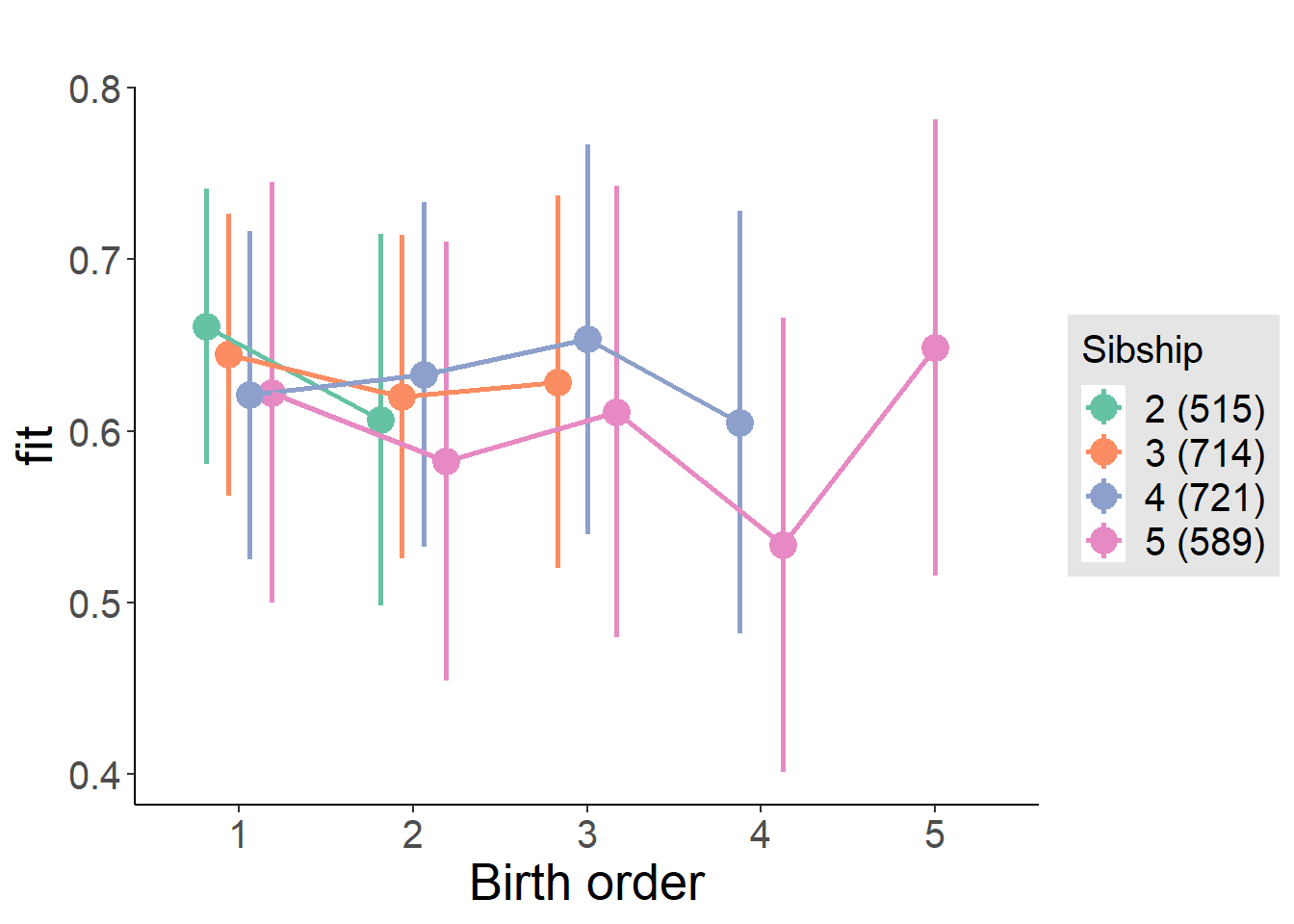
Model Comparison
###### Model 1 - Model 2
anova(m1_covariates_only, m2_birthorder_linear, m3_birthorder_nonlinear, m4_interaction)## refitting model(s) with ML (instead of REML)| Df | AIC | BIC | logLik | deviance | Chisq | Chi Df | Pr(>Chisq) |
|---|---|---|---|---|---|---|---|
| 10 | 3557 | 3616 | -1769 | 3537 | NA | NA | NA |
| 11 | 3559 | 3623 | -1768 | 3537 | 0.2291 | 1 | 0.6322 |
| 14 | 3560 | 3642 | -1766 | 3532 | 4.582 | 3 | 0.2051 |
| 20 | 3570 | 3687 | -1765 | 3530 | 1.837 | 6 | 0.9341 |
Parental full sibling order
outcome_parental_m1 <- update(m2_birthorder_linear, data = birthorder %>%
mutate(sibling_count = sibling_count_genes_factor,
birth_order_nonlinear = birthorder_genes_factor,
birth_order = birthorder_genes,
count_birth_order = count_birthorder_genes
) %>%
filter(sibling_count != "1"))
compare_models_markdown(outcome_parental_m1)Basic Model
Model Summary
m1_covariates_only <- update(m2_birthorder_linear, formula = . ~ . - birth_order)
tidy(m1_covariates_only, conf.int = T, conf.level = 0.995)| effect | group | term | estimate | std.error | statistic | df | p.value | conf.low | conf.high |
|---|---|---|---|---|---|---|---|---|---|
| fixed | NA | (Intercept) | -2.586 | 0.4054 | -6.378 | 2759 | 0.0000000002095 | -3.724 | -1.448 |
| fixed | NA | poly(age, 3, raw = TRUE)1 | 0.3362 | 0.04502 | 7.468 | 2760 | 1.084e-13 | 0.2099 | 0.4626 |
| fixed | NA | poly(age, 3, raw = TRUE)2 | -0.01114 | 0.0016 | -6.959 | 2760 | 4.262e-12 | -0.01563 | -0.006645 |
| fixed | NA | poly(age, 3, raw = TRUE)3 | 0.0001146 | 0.00001822 | 6.291 | 2760 | 0.0000000003657 | 0.00006349 | 0.0001658 |
| fixed | NA | male | 0.02311 | 0.01873 | 1.234 | 2707 | 0.2174 | -0.02947 | 0.07569 |
| fixed | NA | sibling_count3 | -0.0436 | 0.02621 | -1.663 | 2193 | 0.09641 | -0.1172 | 0.02998 |
| fixed | NA | sibling_count4 | -0.03624 | 0.02763 | -1.312 | 2051 | 0.1898 | -0.1138 | 0.04131 |
| fixed | NA | sibling_count5 | -0.07538 | 0.03172 | -2.376 | 1788 | 0.0176 | -0.1644 | 0.01367 |
| ran_pars | mother_pidlink | sd__(Intercept) | 0.2092 | NA | NA | NA | NA | NA | NA |
| ran_pars | Residual | sd__Observation | 0.4434 | NA | NA | NA | NA | NA | NA |
Coefficient Plot
plot(allEffects(m1_covariates_only, confidence.level = 0.995))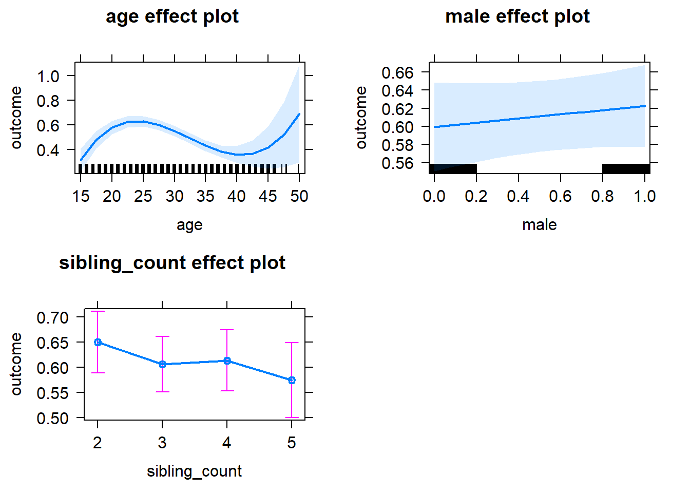
Add Birth Order Linear
Model Summary
tidy(m2_birthorder_linear, conf.int = T, conf.level = 0.995)| effect | group | term | estimate | std.error | statistic | df | p.value | conf.low | conf.high |
|---|---|---|---|---|---|---|---|---|---|
| fixed | NA | (Intercept) | -2.582 | 0.4055 | -6.369 | 2759 | 0.000000000222 | -3.72 | -1.444 |
| fixed | NA | birth_order | -0.007298 | 0.009491 | -0.7689 | 2546 | 0.442 | -0.03394 | 0.01934 |
| fixed | NA | poly(age, 3, raw = TRUE)1 | 0.3368 | 0.04503 | 7.479 | 2759 | 1.002e-13 | 0.2104 | 0.4632 |
| fixed | NA | poly(age, 3, raw = TRUE)2 | -0.01114 | 0.0016 | -6.963 | 2759 | 4.141e-12 | -0.01564 | -0.006652 |
| fixed | NA | poly(age, 3, raw = TRUE)3 | 0.0001145 | 0.00001823 | 6.284 | 2759 | 0.0000000003813 | 0.00006338 | 0.0001657 |
| fixed | NA | male | 0.02304 | 0.01873 | 1.23 | 2706 | 0.2189 | -0.02955 | 0.07562 |
| fixed | NA | sibling_count3 | -0.04001 | 0.02663 | -1.502 | 2222 | 0.1331 | -0.1148 | 0.03474 |
| fixed | NA | sibling_count4 | -0.02877 | 0.02928 | -0.9824 | 2175 | 0.326 | -0.111 | 0.05344 |
| fixed | NA | sibling_count5 | -0.06312 | 0.03551 | -1.777 | 2070 | 0.07565 | -0.1628 | 0.03656 |
| ran_pars | mother_pidlink | sd__(Intercept) | 0.2091 | NA | NA | NA | NA | NA | NA |
| ran_pars | Residual | sd__Observation | 0.4435 | NA | NA | NA | NA | NA | NA |
Coefficient Plot
plot_birthorder2(m2_birthorder_linear, separate = FALSE)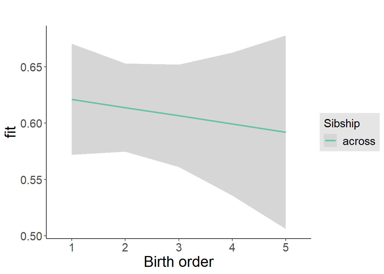
Add Birth Order Factor
Model Summary
m3_birthorder_nonlinear = update(m1_covariates_only, formula = . ~ . + birth_order_nonlinear)
tidy(m3_birthorder_nonlinear, conf.int = T, conf.level = 0.995)| effect | group | term | estimate | std.error | statistic | df | p.value | conf.low | conf.high |
|---|---|---|---|---|---|---|---|---|---|
| fixed | NA | (Intercept) | -2.609 | 0.4061 | -6.424 | 2755 | 0.0000000001555 | -3.749 | -1.469 |
| fixed | NA | poly(age, 3, raw = TRUE)1 | 0.3393 | 0.0451 | 7.525 | 2756 | 7.108e-14 | 0.2127 | 0.4659 |
| fixed | NA | poly(age, 3, raw = TRUE)2 | -0.01123 | 0.001603 | -7.008 | 2756 | 3.034e-12 | -0.01573 | -0.006732 |
| fixed | NA | poly(age, 3, raw = TRUE)3 | 0.0001155 | 0.00001825 | 6.327 | 2756 | 0.0000000002906 | 0.00006424 | 0.0001667 |
| fixed | NA | male | 0.024 | 0.01874 | 1.28 | 2705 | 0.2006 | -0.02862 | 0.07661 |
| fixed | NA | sibling_count3 | -0.04452 | 0.02702 | -1.648 | 2282 | 0.09953 | -0.1204 | 0.03132 |
| fixed | NA | sibling_count4 | -0.02571 | 0.02964 | -0.8673 | 2229 | 0.3859 | -0.1089 | 0.05749 |
| fixed | NA | sibling_count5 | -0.06802 | 0.03606 | -1.886 | 2126 | 0.05937 | -0.1692 | 0.03319 |
| fixed | NA | birth_order_nonlinear2 | -0.02078 | 0.02203 | -0.9431 | 2280 | 0.3457 | -0.08263 | 0.04107 |
| fixed | NA | birth_order_nonlinear3 | 0.002846 | 0.02716 | 0.1048 | 2349 | 0.9165 | -0.07339 | 0.07908 |
| fixed | NA | birth_order_nonlinear4 | -0.06343 | 0.0372 | -1.705 | 2405 | 0.08831 | -0.1678 | 0.04099 |
| fixed | NA | birth_order_nonlinear5 | 0.01625 | 0.05858 | 0.2775 | 2341 | 0.7815 | -0.1482 | 0.1807 |
| ran_pars | mother_pidlink | sd__(Intercept) | 0.2091 | NA | NA | NA | NA | NA | NA |
| ran_pars | Residual | sd__Observation | 0.4434 | NA | NA | NA | NA | NA | NA |
Coefficient Plot
plot_birthorder(m3_birthorder_nonlinear, separate = FALSE)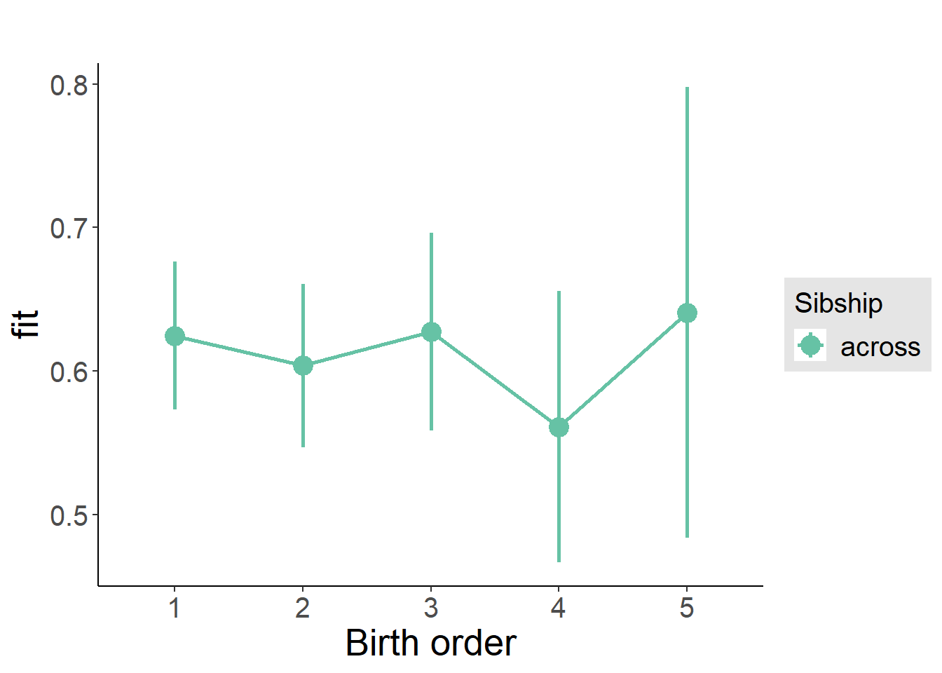
Add Interaction
Model Summary
m4_interaction = update(m3_birthorder_nonlinear, formula = . ~ . - birth_order_nonlinear - sibling_count + count_birth_order)
tidy(m4_interaction, conf.int = T, conf.level = 0.995)| effect | group | term | estimate | std.error | statistic | df | p.value | conf.low | conf.high |
|---|---|---|---|---|---|---|---|---|---|
| fixed | NA | (Intercept) | -2.614 | 0.4067 | -6.427 | 2749 | 0.0000000001531 | -3.755 | -1.472 |
| fixed | NA | poly(age, 3, raw = TRUE)1 | 0.3397 | 0.04516 | 7.523 | 2750 | 7.208e-14 | 0.213 | 0.4665 |
| fixed | NA | poly(age, 3, raw = TRUE)2 | -0.01125 | 0.001605 | -7.007 | 2750 | 3.047e-12 | -0.01575 | -0.006742 |
| fixed | NA | poly(age, 3, raw = TRUE)3 | 0.0001157 | 0.00001828 | 6.329 | 2750 | 0.0000000002874 | 0.00006438 | 0.000167 |
| fixed | NA | male | 0.02395 | 0.01878 | 1.275 | 2698 | 0.2023 | -0.02876 | 0.07666 |
| fixed | NA | count_birth_order2/2 | -0.01649 | 0.03934 | -0.4192 | 2351 | 0.6751 | -0.1269 | 0.09394 |
| fixed | NA | count_birth_order1/3 | -0.0441 | 0.0341 | -1.294 | 2744 | 0.1959 | -0.1398 | 0.0516 |
| fixed | NA | count_birth_order2/3 | -0.06242 | 0.03785 | -1.649 | 2749 | 0.09924 | -0.1687 | 0.04383 |
| fixed | NA | count_birth_order3/3 | -0.04046 | 0.04049 | -0.9991 | 2742 | 0.3178 | -0.1541 | 0.07321 |
| fixed | NA | count_birth_order1/4 | -0.0145 | 0.04006 | -0.362 | 2750 | 0.7174 | -0.127 | 0.09795 |
| fixed | NA | count_birth_order2/4 | -0.03479 | 0.04175 | -0.8331 | 2744 | 0.4048 | -0.152 | 0.08242 |
| fixed | NA | count_birth_order3/4 | -0.03409 | 0.04372 | -0.7797 | 2732 | 0.4356 | -0.1568 | 0.08863 |
| fixed | NA | count_birth_order4/4 | -0.1044 | 0.04709 | -2.217 | 2726 | 0.02674 | -0.2366 | 0.02781 |
| fixed | NA | count_birth_order1/5 | -0.07888 | 0.05248 | -1.503 | 2747 | 0.133 | -0.2262 | 0.06844 |
| fixed | NA | count_birth_order2/5 | -0.1248 | 0.05864 | -2.128 | 2700 | 0.03346 | -0.2894 | 0.03984 |
| fixed | NA | count_birth_order3/5 | -0.04011 | 0.05608 | -0.7152 | 2704 | 0.4746 | -0.1975 | 0.1173 |
| fixed | NA | count_birth_order4/5 | -0.1071 | 0.05404 | -1.983 | 2709 | 0.04748 | -0.2588 | 0.04454 |
| fixed | NA | count_birth_order5/5 | -0.05007 | 0.05685 | -0.8807 | 2701 | 0.3786 | -0.2097 | 0.1095 |
| ran_pars | mother_pidlink | sd__(Intercept) | 0.209 | NA | NA | NA | NA | NA | NA |
| ran_pars | Residual | sd__Observation | 0.4439 | NA | NA | NA | NA | NA | NA |
Coefficient Plot
plot_birthorder(m4_interaction)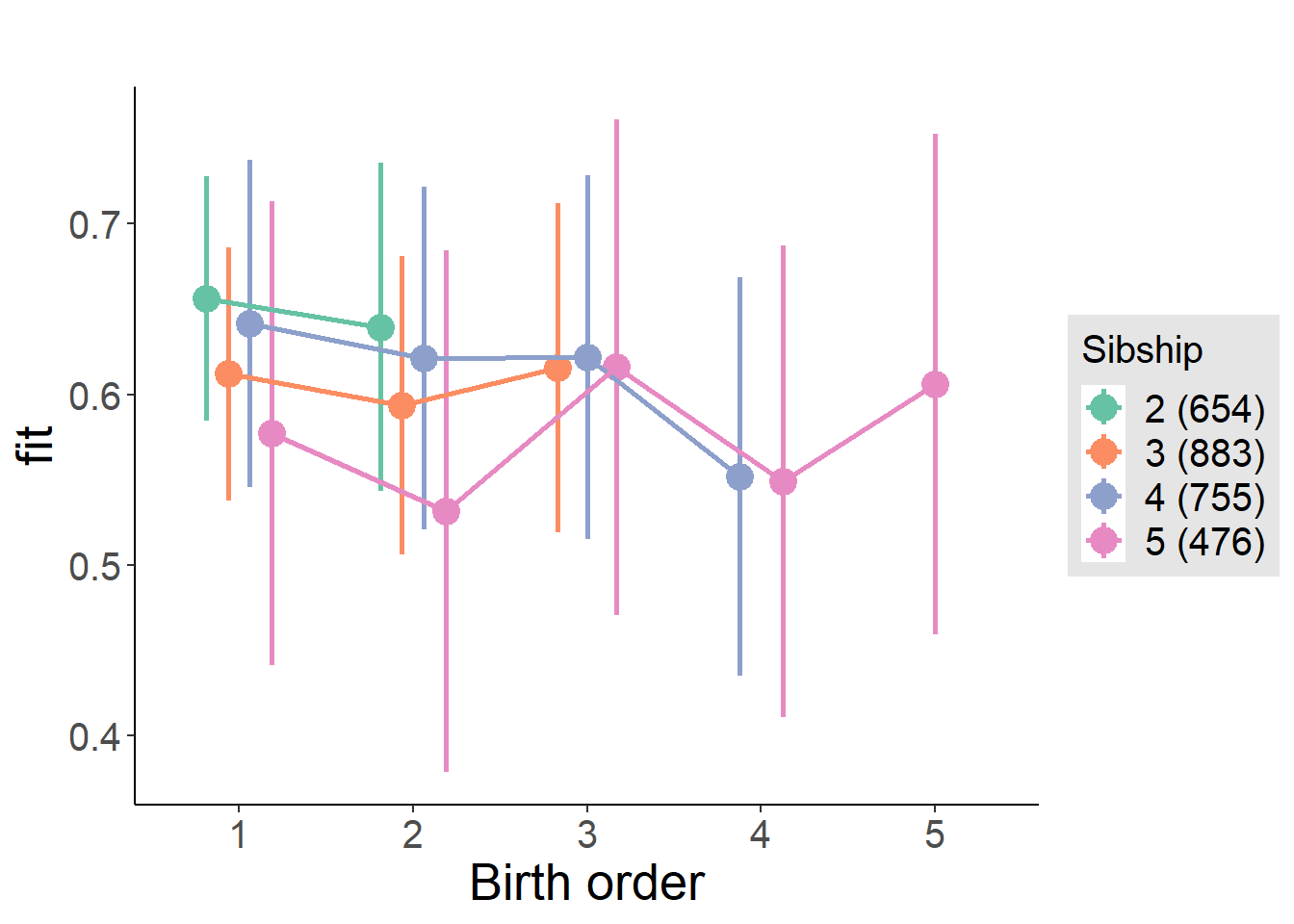
Model Comparison
###### Model 1 - Model 2
anova(m1_covariates_only, m2_birthorder_linear, m3_birthorder_nonlinear, m4_interaction)## refitting model(s) with ML (instead of REML)| Df | AIC | BIC | logLik | deviance | Chisq | Chi Df | Pr(>Chisq) |
|---|---|---|---|---|---|---|---|
| 10 | 3892 | 3951 | -1936 | 3872 | NA | NA | NA |
| 11 | 3894 | 3959 | -1936 | 3872 | 0.5933 | 1 | 0.4411 |
| 14 | 3896 | 3979 | -1934 | 3868 | 3.75 | 3 | 0.2897 |
| 20 | 3906 | 4025 | -1933 | 3866 | 1.579 | 6 | 0.9541 |
Compare birth order specifications
library(coefplot)
multiplot(outcome_naive_m1, outcome_preg_m1, outcome_uterus_m1, outcome_parental_m1, dodgeHeight = 0.6,
intercept = FALSE)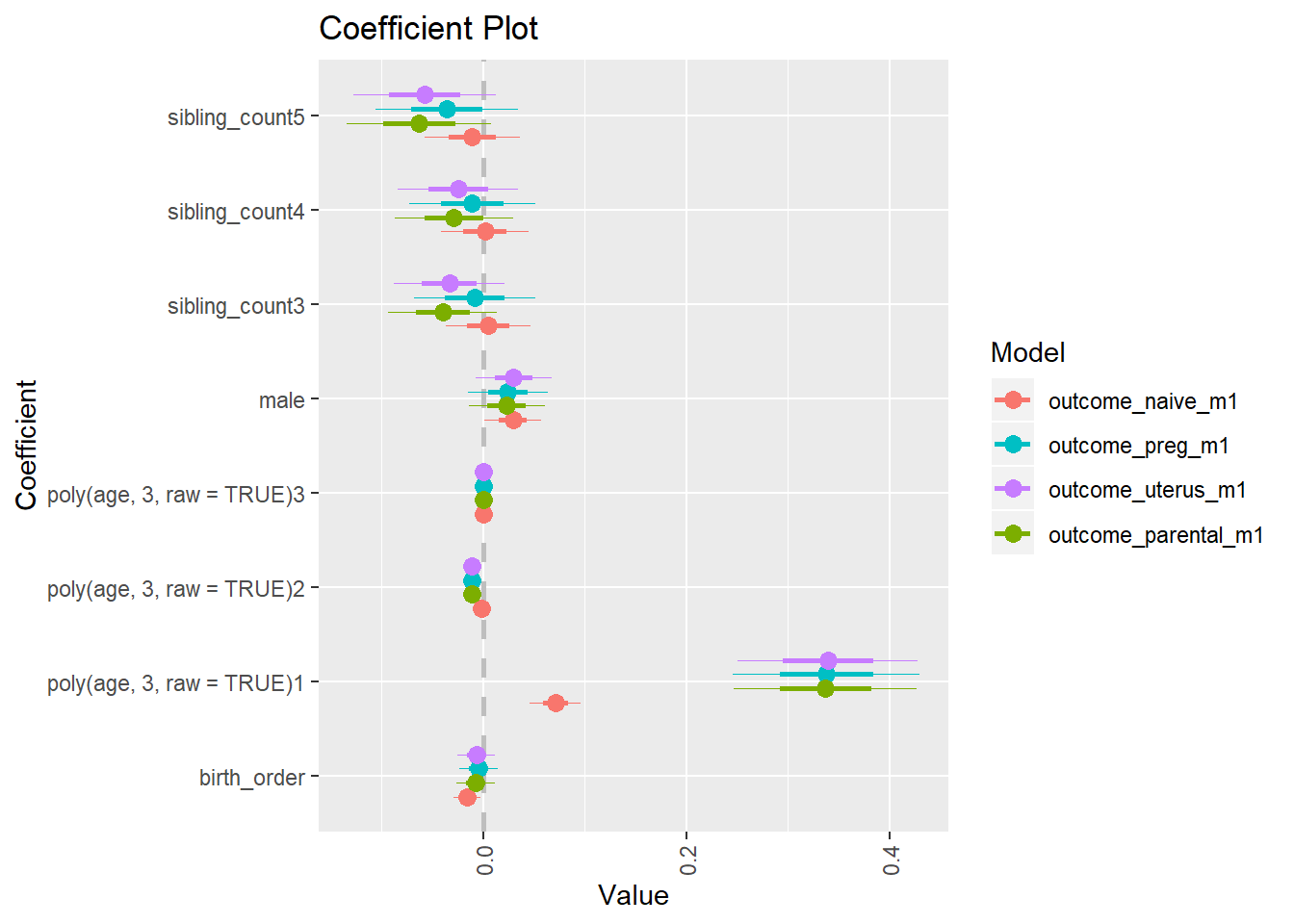
Category_Self-employed
birthorder <- birthorder %>% mutate(outcome = `Category_Self-employed`)
model = lmer(outcome ~ birth_order + poly(age, 3, raw = TRUE) + male + sibling_count + (1 | mother_pidlink),
data = birthorder)
compare_birthorder_specs(model)Naive birth order
outcome_naive_m1 <- update(m2_birthorder_linear, data = birthorder %>%
mutate(sibling_count = sibling_count_naive_factor,
birth_order_nonlinear = birthorder_naive_factor,
birth_order = birthorder_naive,
count_birth_order = count_birthorder_naive) %>%
filter(sibling_count != "1"))
compare_models_markdown(outcome_naive_m1)Basic Model
Model Summary
m1_covariates_only <- update(m2_birthorder_linear, formula = . ~ . - birth_order)
tidy(m1_covariates_only, conf.int = T, conf.level = 0.995)| effect | group | term | estimate | std.error | statistic | df | p.value | conf.low | conf.high |
|---|---|---|---|---|---|---|---|---|---|
| fixed | NA | (Intercept) | -0.1206 | 0.1226 | -0.9834 | 4493 | 0.3255 | -0.4647 | 0.2236 |
| fixed | NA | poly(age, 3, raw = TRUE)1 | 0.012 | 0.01094 | 1.097 | 4392 | 0.2727 | -0.01871 | 0.04271 |
| fixed | NA | poly(age, 3, raw = TRUE)2 | 0.0001217 | 0.0003039 | 0.4005 | 4271 | 0.6888 | -0.0007313 | 0.0009746 |
| fixed | NA | poly(age, 3, raw = TRUE)3 | -0.000002423 | 0.000002658 | -0.9116 | 4161 | 0.3621 | -0.000009883 | 0.000005038 |
| fixed | NA | male | -0.007402 | 0.0124 | -0.5968 | 4755 | 0.5507 | -0.04222 | 0.02741 |
| fixed | NA | sibling_count3 | -0.02237 | 0.01799 | -1.243 | 3513 | 0.2138 | -0.07286 | 0.02813 |
| fixed | NA | sibling_count4 | -0.01961 | 0.0182 | -1.078 | 3307 | 0.2812 | -0.07069 | 0.03147 |
| fixed | NA | sibling_count5 | -0.009391 | 0.019 | -0.4943 | 3086 | 0.6211 | -0.06272 | 0.04394 |
| ran_pars | mother_pidlink | sd__(Intercept) | 0.1564 | NA | NA | NA | NA | NA | NA |
| ran_pars | Residual | sd__Observation | 0.3995 | NA | NA | NA | NA | NA | NA |
Coefficient Plot
plot(allEffects(m1_covariates_only, confidence.level = 0.995))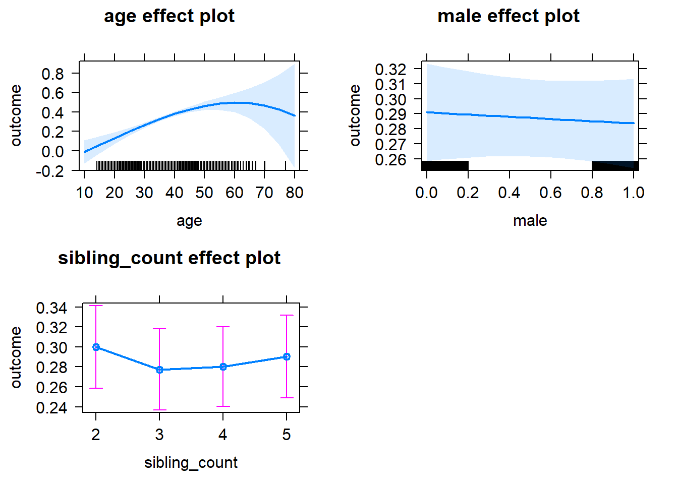
Add Birth Order Linear
Model Summary
tidy(m2_birthorder_linear, conf.int = T, conf.level = 0.995)| effect | group | term | estimate | std.error | statistic | df | p.value | conf.low | conf.high |
|---|---|---|---|---|---|---|---|---|---|
| fixed | NA | (Intercept) | -0.1194 | 0.1226 | -0.9736 | 4493 | 0.3303 | -0.4635 | 0.2248 |
| fixed | NA | birth_order | 0.006512 | 0.006069 | 1.073 | 4244 | 0.2833 | -0.01052 | 0.02355 |
| fixed | NA | poly(age, 3, raw = TRUE)1 | 0.01103 | 0.01098 | 1.005 | 4392 | 0.3151 | -0.01978 | 0.04184 |
| fixed | NA | poly(age, 3, raw = TRUE)2 | 0.0001463 | 0.0003047 | 0.4803 | 4262 | 0.6311 | -0.000709 | 0.001002 |
| fixed | NA | poly(age, 3, raw = TRUE)3 | -0.000002589 | 0.000002662 | -0.9726 | 4153 | 0.3308 | -0.00001006 | 0.000004884 |
| fixed | NA | male | -0.007341 | 0.0124 | -0.5919 | 4754 | 0.554 | -0.04215 | 0.02747 |
| fixed | NA | sibling_count3 | -0.02483 | 0.01813 | -1.369 | 3598 | 0.171 | -0.07573 | 0.02607 |
| fixed | NA | sibling_count4 | -0.02483 | 0.01884 | -1.318 | 3649 | 0.1874 | -0.07771 | 0.02804 |
| fixed | NA | sibling_count5 | -0.01774 | 0.02053 | -0.8642 | 3771 | 0.3875 | -0.07537 | 0.03989 |
| ran_pars | mother_pidlink | sd__(Intercept) | 0.1564 | NA | NA | NA | NA | NA | NA |
| ran_pars | Residual | sd__Observation | 0.3995 | NA | NA | NA | NA | NA | NA |
Coefficient Plot
plot_birthorder2(m2_birthorder_linear, separate = FALSE)
Add Birth Order Factor
Model Summary
m3_birthorder_nonlinear = update(m1_covariates_only, formula = . ~ . + birth_order_nonlinear)
tidy(m3_birthorder_nonlinear, conf.int = T, conf.level = 0.995)| effect | group | term | estimate | std.error | statistic | df | p.value | conf.low | conf.high |
|---|---|---|---|---|---|---|---|---|---|
| fixed | NA | (Intercept) | -0.1273 | 0.1229 | -1.036 | 4498 | 0.3001 | -0.4723 | 0.2176 |
| fixed | NA | poly(age, 3, raw = TRUE)1 | 0.01147 | 0.01097 | 1.046 | 4389 | 0.2958 | -0.01933 | 0.04228 |
| fixed | NA | poly(age, 3, raw = TRUE)2 | 0.0001204 | 0.0003047 | 0.3952 | 4256 | 0.6927 | -0.0007349 | 0.0009757 |
| fixed | NA | poly(age, 3, raw = TRUE)3 | -0.000002249 | 0.000002663 | -0.8444 | 4140 | 0.3985 | -0.000009726 | 0.000005227 |
| fixed | NA | male | -0.00794 | 0.0124 | -0.6405 | 4750 | 0.5219 | -0.04274 | 0.02686 |
| fixed | NA | sibling_count3 | -0.02604 | 0.01843 | -1.413 | 3746 | 0.1577 | -0.07777 | 0.02568 |
| fixed | NA | sibling_count4 | -0.02219 | 0.01914 | -1.159 | 3802 | 0.2466 | -0.07593 | 0.03155 |
| fixed | NA | sibling_count5 | -0.01043 | 0.02071 | -0.5038 | 3865 | 0.6144 | -0.06857 | 0.04771 |
| fixed | NA | birth_order_nonlinear2 | 0.04641 | 0.01462 | 3.175 | 4168 | 0.001509 | 0.00538 | 0.08745 |
| fixed | NA | birth_order_nonlinear3 | 0.02766 | 0.01859 | 1.488 | 4101 | 0.1369 | -0.02453 | 0.07985 |
| fixed | NA | birth_order_nonlinear4 | 0.01196 | 0.02414 | 0.4955 | 4060 | 0.6203 | -0.0558 | 0.07972 |
| fixed | NA | birth_order_nonlinear5 | 0.009981 | 0.03487 | 0.2862 | 4070 | 0.7747 | -0.08791 | 0.1079 |
| ran_pars | mother_pidlink | sd__(Intercept) | 0.1568 | NA | NA | NA | NA | NA | NA |
| ran_pars | Residual | sd__Observation | 0.3991 | NA | NA | NA | NA | NA | NA |
Coefficient Plot
plot_birthorder(m3_birthorder_nonlinear, separate = FALSE)
Add Interaction
Model Summary
m4_interaction = update(m3_birthorder_nonlinear, formula = . ~ . - birth_order_nonlinear - sibling_count + count_birth_order)
tidy(m4_interaction, conf.int = T, conf.level = 0.995)| effect | group | term | estimate | std.error | statistic | df | p.value | conf.low | conf.high |
|---|---|---|---|---|---|---|---|---|---|
| fixed | NA | (Intercept) | -0.1265 | 0.123 | -1.028 | 4502 | 0.3039 | -0.4718 | 0.2189 |
| fixed | NA | poly(age, 3, raw = TRUE)1 | 0.01062 | 0.01098 | 0.9672 | 4386 | 0.3335 | -0.0202 | 0.04144 |
| fixed | NA | poly(age, 3, raw = TRUE)2 | 0.0001361 | 0.0003048 | 0.4465 | 4253 | 0.6553 | -0.0007194 | 0.0009916 |
| fixed | NA | poly(age, 3, raw = TRUE)3 | -0.000002308 | 0.000002664 | -0.8666 | 4137 | 0.3862 | -0.000009785 | 0.000005168 |
| fixed | NA | male | -0.008281 | 0.0124 | -0.6679 | 4743 | 0.5042 | -0.04309 | 0.02652 |
| fixed | NA | count_birth_order2/2 | 0.07691 | 0.02482 | 3.098 | 4123 | 0.001961 | 0.007225 | 0.1466 |
| fixed | NA | count_birth_order1/3 | -0.02403 | 0.02407 | -0.9984 | 4793 | 0.3182 | -0.09159 | 0.04353 |
| fixed | NA | count_birth_order2/3 | 0.03415 | 0.02669 | 1.28 | 4804 | 0.2008 | -0.04077 | 0.1091 |
| fixed | NA | count_birth_order3/3 | 0.02757 | 0.02937 | 0.9389 | 4806 | 0.3478 | -0.05486 | 0.11 |
| fixed | NA | count_birth_order1/4 | 0.01578 | 0.02638 | 0.5979 | 4804 | 0.5499 | -0.05829 | 0.08984 |
| fixed | NA | count_birth_order2/4 | 0.006164 | 0.0283 | 0.2178 | 4806 | 0.8276 | -0.07327 | 0.0856 |
| fixed | NA | count_birth_order3/4 | -0.003886 | 0.03019 | -0.1287 | 4804 | 0.8976 | -0.08862 | 0.08085 |
| fixed | NA | count_birth_order4/4 | 0.02151 | 0.03211 | 0.67 | 4803 | 0.5029 | -0.06863 | 0.1117 |
| fixed | NA | count_birth_order1/5 | 0.01111 | 0.02995 | 0.3709 | 4804 | 0.7107 | -0.07297 | 0.09518 |
| fixed | NA | count_birth_order2/5 | 0.0492 | 0.03179 | 1.547 | 4801 | 0.1218 | -0.04004 | 0.1384 |
| fixed | NA | count_birth_order3/5 | 0.03627 | 0.03346 | 1.084 | 4796 | 0.2785 | -0.05767 | 0.1302 |
| fixed | NA | count_birth_order4/5 | -0.01264 | 0.03519 | -0.359 | 4775 | 0.7196 | -0.1114 | 0.08615 |
| fixed | NA | count_birth_order5/5 | 0.01104 | 0.03522 | 0.3136 | 4791 | 0.7539 | -0.08782 | 0.1099 |
| ran_pars | mother_pidlink | sd__(Intercept) | 0.1569 | NA | NA | NA | NA | NA | NA |
| ran_pars | Residual | sd__Observation | 0.399 | NA | NA | NA | NA | NA | NA |
Coefficient Plot
plot_birthorder(m4_interaction)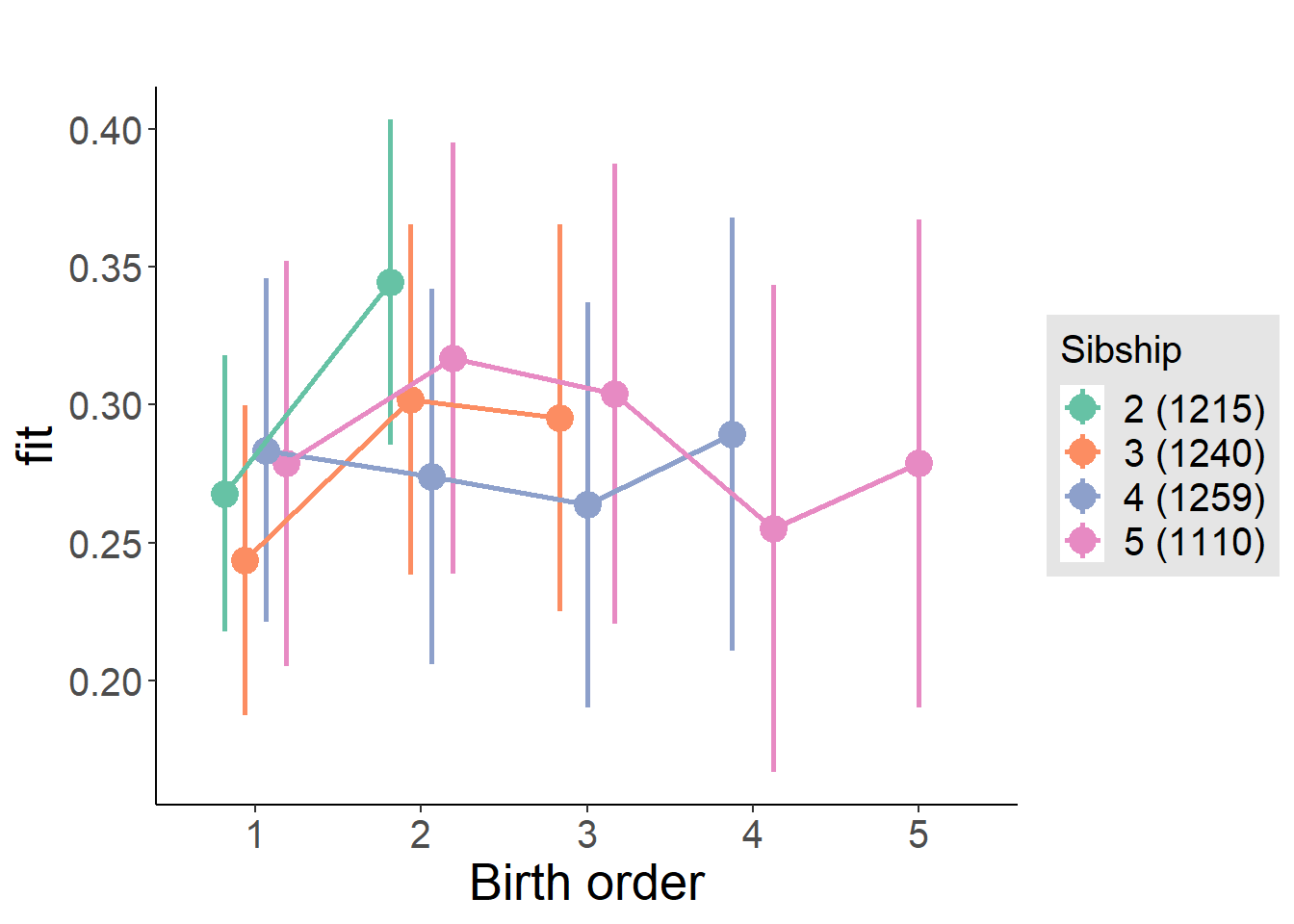
Model Comparison
###### Model 1 - Model 2
anova(m1_covariates_only, m2_birthorder_linear, m3_birthorder_nonlinear, m4_interaction)## refitting model(s) with ML (instead of REML)| Df | AIC | BIC | logLik | deviance | Chisq | Chi Df | Pr(>Chisq) |
|---|---|---|---|---|---|---|---|
| 10 | 5504 | 5569 | -2742 | 5484 | NA | NA | NA |
| 11 | 5505 | 5576 | -2741 | 5483 | 1.154 | 1 | 0.2828 |
| 14 | 5501 | 5592 | -2737 | 5473 | 9.456 | 3 | 0.0238 |
| 20 | 5506 | 5635 | -2733 | 5466 | 7.697 | 6 | 0.2612 |
Maternal birth order
outcome_uterus_m1 <- update(m2_birthorder_linear, data = birthorder %>%
mutate(sibling_count = sibling_count_uterus_alive_factor,
birth_order_nonlinear = birthorder_uterus_alive_factor,
birth_order = birthorder_uterus_alive,
count_birth_order = count_birthorder_uterus_alive) %>%
filter(sibling_count != "1"))
compare_models_markdown(outcome_uterus_m1)Basic Model
Model Summary
m1_covariates_only <- update(m2_birthorder_linear, formula = . ~ . - birth_order)
tidy(m1_covariates_only, conf.int = T, conf.level = 0.995)| effect | group | term | estimate | std.error | statistic | df | p.value | conf.low | conf.high |
|---|---|---|---|---|---|---|---|---|---|
| fixed | NA | (Intercept) | 1.112 | 0.3187 | 3.489 | 2759 | 0.000492 | 0.2174 | 2.007 |
| fixed | NA | poly(age, 3, raw = TRUE)1 | -0.1214 | 0.03531 | -3.439 | 2760 | 0.0005935 | -0.2205 | -0.0223 |
| fixed | NA | poly(age, 3, raw = TRUE)2 | 0.004639 | 0.001252 | 3.705 | 2760 | 0.0002156 | 0.001124 | 0.008154 |
| fixed | NA | poly(age, 3, raw = TRUE)3 | -0.00005136 | 0.00001422 | -3.611 | 2760 | 0.00031 | -0.00009129 | -0.00001144 |
| fixed | NA | male | -0.04191 | 0.0149 | -2.813 | 2721 | 0.004946 | -0.08373 | -0.00008659 |
| fixed | NA | sibling_count3 | 0.01673 | 0.02117 | 0.7903 | 2217 | 0.4294 | -0.04269 | 0.07615 |
| fixed | NA | sibling_count4 | -0.02678 | 0.022 | -1.217 | 2081 | 0.2236 | -0.08852 | 0.03497 |
| fixed | NA | sibling_count5 | 0.04089 | 0.02453 | 1.667 | 1873 | 0.09571 | -0.02797 | 0.1098 |
| ran_pars | mother_pidlink | sd__(Intercept) | 0.157 | NA | NA | NA | NA | NA | NA |
| ran_pars | Residual | sd__Observation | 0.3561 | NA | NA | NA | NA | NA | NA |
Coefficient Plot
plot(allEffects(m1_covariates_only, confidence.level = 0.995))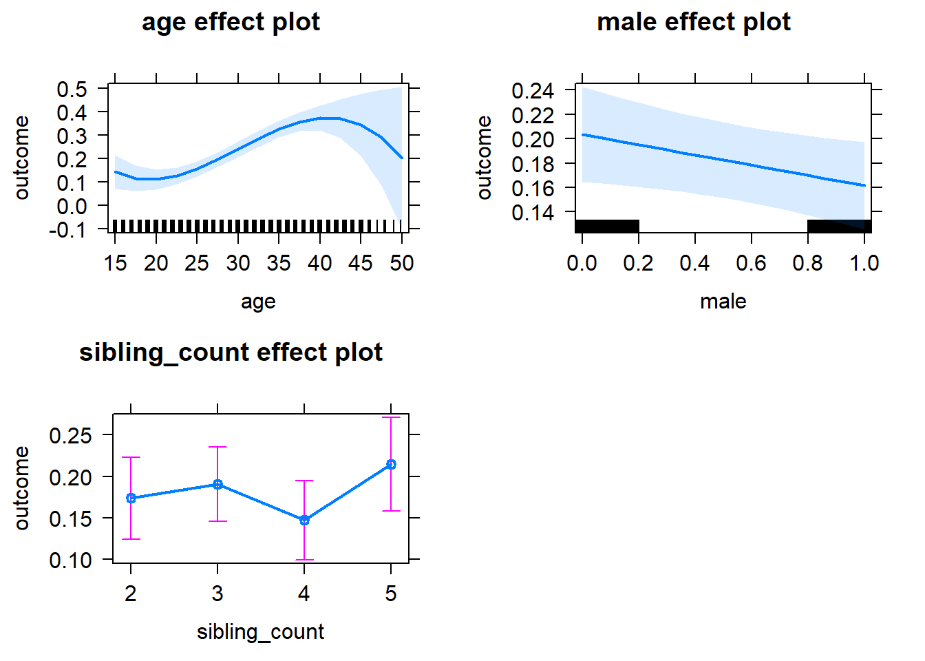
Add Birth Order Linear
Model Summary
tidy(m2_birthorder_linear, conf.int = T, conf.level = 0.995)| effect | group | term | estimate | std.error | statistic | df | p.value | conf.low | conf.high |
|---|---|---|---|---|---|---|---|---|---|
| fixed | NA | (Intercept) | 1.113 | 0.3188 | 3.49 | 2758 | 0.0004908 | 0.2177 | 2.008 |
| fixed | NA | birth_order | -0.001112 | 0.007469 | -0.1489 | 2589 | 0.8816 | -0.02208 | 0.01985 |
| fixed | NA | poly(age, 3, raw = TRUE)1 | -0.1213 | 0.03532 | -3.435 | 2758 | 0.0006009 | -0.2205 | -0.02218 |
| fixed | NA | poly(age, 3, raw = TRUE)2 | 0.004638 | 0.001252 | 3.703 | 2759 | 0.0002169 | 0.001123 | 0.008153 |
| fixed | NA | poly(age, 3, raw = TRUE)3 | -0.00005138 | 0.00001423 | -3.612 | 2759 | 0.0003095 | -0.00009131 | -0.00001145 |
| fixed | NA | male | -0.04191 | 0.0149 | -2.812 | 2720 | 0.004953 | -0.08374 | -0.00007972 |
| fixed | NA | sibling_count3 | 0.01727 | 0.02148 | 0.8039 | 2246 | 0.4215 | -0.04303 | 0.07756 |
| fixed | NA | sibling_count4 | -0.02562 | 0.02332 | -1.099 | 2194 | 0.2719 | -0.09108 | 0.03983 |
| fixed | NA | sibling_count5 | 0.04282 | 0.02776 | 1.543 | 2169 | 0.123 | -0.03509 | 0.1207 |
| ran_pars | mother_pidlink | sd__(Intercept) | 0.1571 | NA | NA | NA | NA | NA | NA |
| ran_pars | Residual | sd__Observation | 0.3561 | NA | NA | NA | NA | NA | NA |
Coefficient Plot
plot_birthorder2(m2_birthorder_linear, separate = FALSE)
Add Birth Order Factor
Model Summary
m3_birthorder_nonlinear = update(m1_covariates_only, formula = . ~ . + birth_order_nonlinear)
tidy(m3_birthorder_nonlinear, conf.int = T, conf.level = 0.995)| effect | group | term | estimate | std.error | statistic | df | p.value | conf.low | conf.high |
|---|---|---|---|---|---|---|---|---|---|
| fixed | NA | (Intercept) | 1.113 | 0.3195 | 3.483 | 2755 | 0.0005044 | 0.2159 | 2.01 |
| fixed | NA | poly(age, 3, raw = TRUE)1 | -0.1218 | 0.03539 | -3.443 | 2755 | 0.0005845 | -0.2212 | -0.0225 |
| fixed | NA | poly(age, 3, raw = TRUE)2 | 0.004652 | 0.001255 | 3.708 | 2756 | 0.0002134 | 0.00113 | 0.008175 |
| fixed | NA | poly(age, 3, raw = TRUE)3 | -0.00005151 | 0.00001425 | -3.614 | 2756 | 0.0003066 | -0.00009151 | -0.0000115 |
| fixed | NA | male | -0.04216 | 0.01491 | -2.827 | 2718 | 0.004737 | -0.08402 | -0.0002938 |
| fixed | NA | sibling_count3 | 0.01836 | 0.02179 | 0.8423 | 2302 | 0.3997 | -0.04282 | 0.07954 |
| fixed | NA | sibling_count4 | -0.02705 | 0.02361 | -1.146 | 2246 | 0.252 | -0.09334 | 0.03923 |
| fixed | NA | sibling_count5 | 0.0469 | 0.0281 | 1.669 | 2210 | 0.09523 | -0.03198 | 0.1258 |
| fixed | NA | birth_order_nonlinear2 | 0.01228 | 0.01776 | 0.691 | 2336 | 0.4896 | -0.03759 | 0.06214 |
| fixed | NA | birth_order_nonlinear3 | -0.005867 | 0.02171 | -0.2702 | 2396 | 0.787 | -0.06681 | 0.05508 |
| fixed | NA | birth_order_nonlinear4 | 0.01255 | 0.02887 | 0.4346 | 2459 | 0.6639 | -0.06849 | 0.09359 |
| fixed | NA | birth_order_nonlinear5 | -0.02938 | 0.0443 | -0.6631 | 2389 | 0.5073 | -0.1537 | 0.09498 |
| ran_pars | mother_pidlink | sd__(Intercept) | 0.1575 | NA | NA | NA | NA | NA | NA |
| ran_pars | Residual | sd__Observation | 0.3561 | NA | NA | NA | NA | NA | NA |
Coefficient Plot
plot_birthorder(m3_birthorder_nonlinear, separate = FALSE)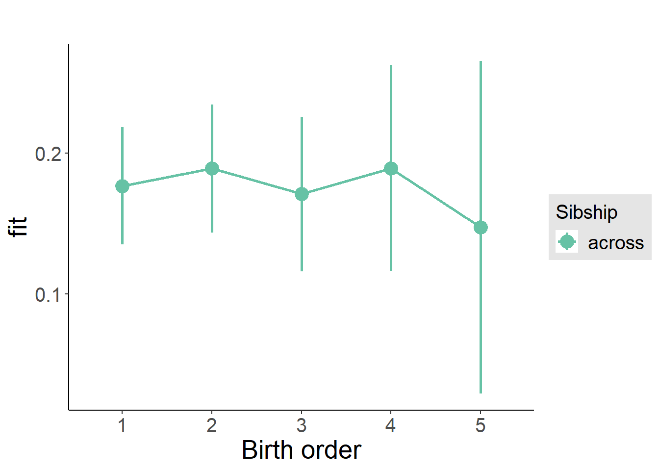
Add Interaction
Model Summary
m4_interaction = update(m3_birthorder_nonlinear, formula = . ~ . - birth_order_nonlinear - sibling_count + count_birth_order)
tidy(m4_interaction, conf.int = T, conf.level = 0.995)| effect | group | term | estimate | std.error | statistic | df | p.value | conf.low | conf.high |
|---|---|---|---|---|---|---|---|---|---|
| fixed | NA | (Intercept) | 1.101 | 0.3199 | 3.443 | 2749 | 0.0005833 | 0.2035 | 1.999 |
| fixed | NA | poly(age, 3, raw = TRUE)1 | -0.122 | 0.03542 | -3.443 | 2749 | 0.0005832 | -0.2214 | -0.02254 |
| fixed | NA | poly(age, 3, raw = TRUE)2 | 0.004655 | 0.001256 | 3.706 | 2750 | 0.0002145 | 0.001129 | 0.008181 |
| fixed | NA | poly(age, 3, raw = TRUE)3 | -0.00005152 | 0.00001427 | -3.611 | 2750 | 0.0003104 | -0.00009157 | -0.00001147 |
| fixed | NA | male | -0.04244 | 0.01494 | -2.841 | 2712 | 0.00453 | -0.08437 | -0.0005087 |
| fixed | NA | count_birth_order2/2 | 0.0532 | 0.03229 | 1.648 | 2406 | 0.09955 | -0.03743 | 0.1438 |
| fixed | NA | count_birth_order1/3 | 0.04188 | 0.02754 | 1.52 | 2745 | 0.1285 | -0.03544 | 0.1192 |
| fixed | NA | count_birth_order2/3 | 0.03959 | 0.03056 | 1.296 | 2750 | 0.1952 | -0.04619 | 0.1254 |
| fixed | NA | count_birth_order3/3 | 0.01101 | 0.03305 | 0.3331 | 2746 | 0.7391 | -0.08175 | 0.1038 |
| fixed | NA | count_birth_order1/4 | -0.006186 | 0.03172 | -0.195 | 2749 | 0.8454 | -0.09522 | 0.08285 |
| fixed | NA | count_birth_order2/4 | -0.02662 | 0.03329 | -0.7996 | 2747 | 0.424 | -0.1201 | 0.06682 |
| fixed | NA | count_birth_order3/4 | -0.01179 | 0.03488 | -0.338 | 2737 | 0.7354 | -0.1097 | 0.08611 |
| fixed | NA | count_birth_order4/4 | 0.01099 | 0.03695 | 0.2973 | 2735 | 0.7663 | -0.09273 | 0.1147 |
| fixed | NA | count_birth_order1/5 | 0.05724 | 0.04167 | 1.374 | 2747 | 0.1697 | -0.05974 | 0.1742 |
| fixed | NA | count_birth_order2/5 | 0.07863 | 0.04519 | 1.74 | 2719 | 0.08198 | -0.04822 | 0.2055 |
| fixed | NA | count_birth_order3/5 | 0.06885 | 0.0423 | 1.628 | 2724 | 0.1037 | -0.04988 | 0.1876 |
| fixed | NA | count_birth_order4/5 | 0.05676 | 0.0411 | 1.381 | 2722 | 0.1674 | -0.0586 | 0.1721 |
| fixed | NA | count_birth_order5/5 | 0.03067 | 0.04307 | 0.712 | 2715 | 0.4765 | -0.09024 | 0.1516 |
| ran_pars | mother_pidlink | sd__(Intercept) | 0.1566 | NA | NA | NA | NA | NA | NA |
| ran_pars | Residual | sd__Observation | 0.3566 | NA | NA | NA | NA | NA | NA |
Coefficient Plot
plot_birthorder(m4_interaction)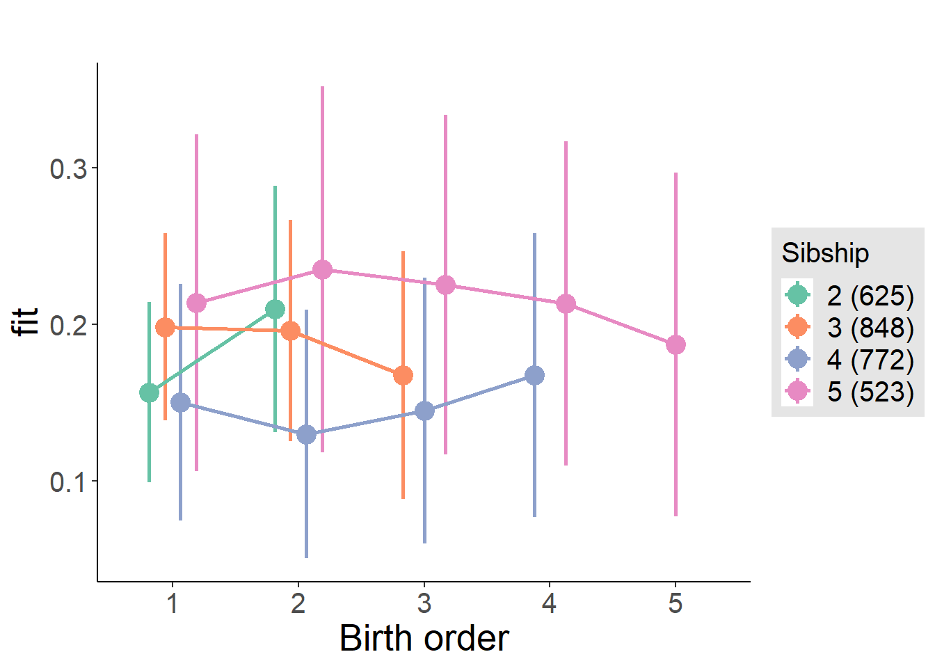
Model Comparison
###### Model 1 - Model 2
anova(m1_covariates_only, m2_birthorder_linear, m3_birthorder_nonlinear, m4_interaction)## refitting model(s) with ML (instead of REML)| Df | AIC | BIC | logLik | deviance | Chisq | Chi Df | Pr(>Chisq) |
|---|---|---|---|---|---|---|---|
| 10 | 2619 | 2678 | -1300 | 2599 | NA | NA | NA |
| 11 | 2621 | 2686 | -1300 | 2599 | 0.02164 | 1 | 0.8831 |
| 14 | 2626 | 2709 | -1299 | 2598 | 1.583 | 3 | 0.6632 |
| 20 | 2634 | 2752 | -1297 | 2594 | 3.881 | 6 | 0.6928 |
Maternal pregnancy order
outcome_preg_m1 <- update(m2_birthorder_linear, data = birthorder %>%
mutate(sibling_count = sibling_count_uterus_preg_factor,
birth_order_nonlinear = birthorder_uterus_preg_factor,
birth_order = birthorder_uterus_preg,
count_birth_order = count_birthorder_uterus_preg
) %>%
filter(sibling_count != "1"))
compare_models_markdown(outcome_preg_m1)Basic Model
Model Summary
m1_covariates_only <- update(m2_birthorder_linear, formula = . ~ . - birth_order)
tidy(m1_covariates_only, conf.int = T, conf.level = 0.995)| effect | group | term | estimate | std.error | statistic | df | p.value | conf.low | conf.high |
|---|---|---|---|---|---|---|---|---|---|
| fixed | NA | (Intercept) | 1.049 | 0.3272 | 3.207 | 2531 | 0.001358 | 0.1308 | 1.968 |
| fixed | NA | poly(age, 3, raw = TRUE)1 | -0.1131 | 0.03626 | -3.118 | 2531 | 0.00184 | -0.2148 | -0.01128 |
| fixed | NA | poly(age, 3, raw = TRUE)2 | 0.00436 | 0.001286 | 3.39 | 2531 | 0.0007086 | 0.0007501 | 0.007969 |
| fixed | NA | poly(age, 3, raw = TRUE)3 | -0.00004835 | 0.00001461 | -3.31 | 2531 | 0.0009454 | -0.00008935 | -0.00000735 |
| fixed | NA | male | -0.04432 | 0.01541 | -2.877 | 2482 | 0.004054 | -0.08756 | -0.001071 |
| fixed | NA | sibling_count3 | -0.004593 | 0.02309 | -0.1989 | 2047 | 0.8424 | -0.06942 | 0.06023 |
| fixed | NA | sibling_count4 | -0.03224 | 0.02342 | -1.377 | 1966 | 0.1688 | -0.09797 | 0.0335 |
| fixed | NA | sibling_count5 | -0.005695 | 0.02477 | -0.2299 | 1839 | 0.8182 | -0.07524 | 0.06385 |
| ran_pars | mother_pidlink | sd__(Intercept) | 0.1675 | NA | NA | NA | NA | NA | NA |
| ran_pars | Residual | sd__Observation | 0.3479 | NA | NA | NA | NA | NA | NA |
Coefficient Plot
plot(allEffects(m1_covariates_only, confidence.level = 0.995))
Add Birth Order Linear
Model Summary
tidy(m2_birthorder_linear, conf.int = T, conf.level = 0.995)| effect | group | term | estimate | std.error | statistic | df | p.value | conf.low | conf.high |
|---|---|---|---|---|---|---|---|---|---|
| fixed | NA | (Intercept) | 1.05 | 0.3273 | 3.207 | 2530 | 0.001357 | 0.131 | 1.968 |
| fixed | NA | birth_order | -0.0005907 | 0.007493 | -0.07884 | 2399 | 0.9372 | -0.02162 | 0.02044 |
| fixed | NA | poly(age, 3, raw = TRUE)1 | -0.113 | 0.03627 | -3.117 | 2530 | 0.001848 | -0.2148 | -0.01124 |
| fixed | NA | poly(age, 3, raw = TRUE)2 | 0.004359 | 0.001286 | 3.39 | 2530 | 0.0007105 | 0.0007493 | 0.00797 |
| fixed | NA | poly(age, 3, raw = TRUE)3 | -0.00004837 | 0.00001461 | -3.31 | 2530 | 0.0009453 | -0.00008938 | -0.000007352 |
| fixed | NA | male | -0.04433 | 0.01541 | -2.877 | 2481 | 0.004051 | -0.08759 | -0.001076 |
| fixed | NA | sibling_count3 | -0.004297 | 0.0234 | -0.1836 | 2064 | 0.8543 | -0.06998 | 0.06139 |
| fixed | NA | sibling_count4 | -0.03166 | 0.02453 | -1.291 | 2036 | 0.1969 | -0.1005 | 0.03719 |
| fixed | NA | sibling_count5 | -0.004735 | 0.02761 | -0.1715 | 2046 | 0.8639 | -0.08223 | 0.07276 |
| ran_pars | mother_pidlink | sd__(Intercept) | 0.1675 | NA | NA | NA | NA | NA | NA |
| ran_pars | Residual | sd__Observation | 0.3479 | NA | NA | NA | NA | NA | NA |
Coefficient Plot
plot_birthorder2(m2_birthorder_linear, separate = FALSE)
Add Birth Order Factor
Model Summary
m3_birthorder_nonlinear = update(m1_covariates_only, formula = . ~ . + birth_order_nonlinear)
tidy(m3_birthorder_nonlinear, conf.int = T, conf.level = 0.995)| effect | group | term | estimate | std.error | statistic | df | p.value | conf.low | conf.high |
|---|---|---|---|---|---|---|---|---|---|
| fixed | NA | (Intercept) | 1.054 | 0.3282 | 3.212 | 2527 | 0.001335 | 0.1329 | 1.975 |
| fixed | NA | poly(age, 3, raw = TRUE)1 | -0.1141 | 0.03636 | -3.139 | 2527 | 0.001714 | -0.2162 | -0.01208 |
| fixed | NA | poly(age, 3, raw = TRUE)2 | 0.004394 | 0.001289 | 3.408 | 2527 | 0.0006646 | 0.0007749 | 0.008013 |
| fixed | NA | poly(age, 3, raw = TRUE)3 | -0.00004871 | 0.00001465 | -3.326 | 2527 | 0.0008931 | -0.00008982 | -0.000007603 |
| fixed | NA | male | -0.04453 | 0.01542 | -2.888 | 2478 | 0.003913 | -0.08782 | -0.001246 |
| fixed | NA | sibling_count3 | -0.001584 | 0.02372 | -0.0668 | 2109 | 0.9467 | -0.06817 | 0.065 |
| fixed | NA | sibling_count4 | -0.02968 | 0.02481 | -1.196 | 2077 | 0.2317 | -0.09933 | 0.03997 |
| fixed | NA | sibling_count5 | -0.002534 | 0.02777 | -0.09124 | 2064 | 0.9273 | -0.08049 | 0.07542 |
| fixed | NA | birth_order_nonlinear2 | 0.01805 | 0.01822 | 0.9904 | 2121 | 0.3221 | -0.03311 | 0.06921 |
| fixed | NA | birth_order_nonlinear3 | -0.01218 | 0.02252 | -0.5409 | 2207 | 0.5886 | -0.07539 | 0.05103 |
| fixed | NA | birth_order_nonlinear4 | 0.004847 | 0.02955 | 0.164 | 2254 | 0.8697 | -0.0781 | 0.08779 |
| fixed | NA | birth_order_nonlinear5 | 0.002927 | 0.04218 | 0.06938 | 2178 | 0.9447 | -0.1155 | 0.1213 |
| ran_pars | mother_pidlink | sd__(Intercept) | 0.1676 | NA | NA | NA | NA | NA | NA |
| ran_pars | Residual | sd__Observation | 0.348 | NA | NA | NA | NA | NA | NA |
Coefficient Plot
plot_birthorder(m3_birthorder_nonlinear, separate = FALSE)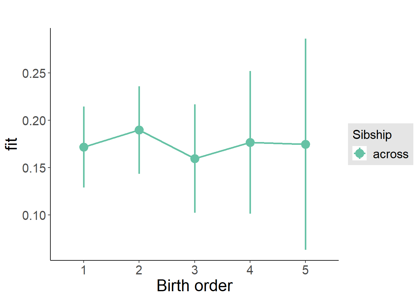
Add Interaction
Model Summary
m4_interaction = update(m3_birthorder_nonlinear, formula = . ~ . - birth_order_nonlinear - sibling_count + count_birth_order)
tidy(m4_interaction, conf.int = T, conf.level = 0.995)| effect | group | term | estimate | std.error | statistic | df | p.value | conf.low | conf.high |
|---|---|---|---|---|---|---|---|---|---|
| fixed | NA | (Intercept) | 1.035 | 0.3284 | 3.15 | 2521 | 0.001649 | 0.1128 | 1.957 |
| fixed | NA | poly(age, 3, raw = TRUE)1 | -0.1142 | 0.03639 | -3.138 | 2521 | 0.001723 | -0.2163 | -0.01203 |
| fixed | NA | poly(age, 3, raw = TRUE)2 | 0.004394 | 0.00129 | 3.405 | 2521 | 0.0006717 | 0.0007717 | 0.008016 |
| fixed | NA | poly(age, 3, raw = TRUE)3 | -0.0000487 | 0.00001466 | -3.323 | 2521 | 0.0009044 | -0.00008985 | -0.000007557 |
| fixed | NA | male | -0.04493 | 0.01545 | -2.908 | 2473 | 0.003673 | -0.0883 | -0.001556 |
| fixed | NA | count_birth_order2/2 | 0.08055 | 0.0351 | 2.295 | 2248 | 0.02183 | -0.01798 | 0.1791 |
| fixed | NA | count_birth_order1/3 | 0.02443 | 0.03018 | 0.8094 | 2515 | 0.4184 | -0.06028 | 0.1091 |
| fixed | NA | count_birth_order2/3 | 0.04417 | 0.03276 | 1.348 | 2521 | 0.1777 | -0.0478 | 0.1361 |
| fixed | NA | count_birth_order3/3 | -0.01421 | 0.03599 | -0.3948 | 2516 | 0.693 | -0.1152 | 0.08682 |
| fixed | NA | count_birth_order1/4 | 0.01002 | 0.0329 | 0.3045 | 2519 | 0.7608 | -0.08234 | 0.1024 |
| fixed | NA | count_birth_order2/4 | -0.0249 | 0.03426 | -0.7267 | 2520 | 0.4675 | -0.1211 | 0.07127 |
| fixed | NA | count_birth_order3/4 | -0.008878 | 0.03737 | -0.2375 | 2505 | 0.8123 | -0.1138 | 0.09603 |
| fixed | NA | count_birth_order4/4 | -0.002061 | 0.03984 | -0.05174 | 2499 | 0.9587 | -0.1139 | 0.1098 |
| fixed | NA | count_birth_order1/5 | 0.02277 | 0.03946 | 0.5769 | 2520 | 0.5641 | -0.08801 | 0.1335 |
| fixed | NA | count_birth_order2/5 | 0.02039 | 0.04089 | 0.4985 | 2508 | 0.6182 | -0.0944 | 0.1352 |
| fixed | NA | count_birth_order3/5 | 0.01907 | 0.04154 | 0.4591 | 2494 | 0.6462 | -0.09754 | 0.1357 |
| fixed | NA | count_birth_order4/5 | 0.01981 | 0.04213 | 0.4702 | 2480 | 0.6383 | -0.09846 | 0.1381 |
| fixed | NA | count_birth_order5/5 | 0.02095 | 0.04244 | 0.4937 | 2480 | 0.6215 | -0.09817 | 0.1401 |
| ran_pars | mother_pidlink | sd__(Intercept) | 0.1668 | NA | NA | NA | NA | NA | NA |
| ran_pars | Residual | sd__Observation | 0.3483 | NA | NA | NA | NA | NA | NA |
Coefficient Plot
plot_birthorder(m4_interaction)
Model Comparison
###### Model 1 - Model 2
anova(m1_covariates_only, m2_birthorder_linear, m3_birthorder_nonlinear, m4_interaction)## refitting model(s) with ML (instead of REML)| Df | AIC | BIC | logLik | deviance | Chisq | Chi Df | Pr(>Chisq) |
|---|---|---|---|---|---|---|---|
| 10 | 2357 | 2415 | -1168 | 2337 | NA | NA | NA |
| 11 | 2359 | 2423 | -1168 | 2337 | 0.006049 | 1 | 0.938 |
| 14 | 2363 | 2445 | -1167 | 2335 | 1.949 | 3 | 0.5831 |
| 20 | 2368 | 2485 | -1164 | 2328 | 6.778 | 6 | 0.3418 |
Parental full sibling order
outcome_parental_m1 <- update(m2_birthorder_linear, data = birthorder %>%
mutate(sibling_count = sibling_count_genes_factor,
birth_order_nonlinear = birthorder_genes_factor,
birth_order = birthorder_genes,
count_birth_order = count_birthorder_genes
) %>%
filter(sibling_count != "1"))
compare_models_markdown(outcome_parental_m1)Basic Model
Model Summary
m1_covariates_only <- update(m2_birthorder_linear, formula = . ~ . - birth_order)
tidy(m1_covariates_only, conf.int = T, conf.level = 0.995)| effect | group | term | estimate | std.error | statistic | df | p.value | conf.low | conf.high |
|---|---|---|---|---|---|---|---|---|---|
| fixed | NA | (Intercept) | 1.218 | 0.3247 | 3.753 | 2759 | 0.0001783 | 0.3071 | 2.13 |
| fixed | NA | poly(age, 3, raw = TRUE)1 | -0.1353 | 0.03606 | -3.752 | 2759 | 0.0001789 | -0.2365 | -0.03408 |
| fixed | NA | poly(age, 3, raw = TRUE)2 | 0.005209 | 0.001282 | 4.064 | 2760 | 0.00004949 | 0.001612 | 0.008807 |
| fixed | NA | poly(age, 3, raw = TRUE)3 | -0.00005869 | 0.0000146 | -4.021 | 2759 | 0.00005948 | -0.00009966 | -0.00001772 |
| fixed | NA | male | -0.03916 | 0.01501 | -2.609 | 2716 | 0.009137 | -0.0813 | 0.002977 |
| fixed | NA | sibling_count3 | 0.02419 | 0.02095 | 1.155 | 2215 | 0.2484 | -0.03461 | 0.08299 |
| fixed | NA | sibling_count4 | -0.02397 | 0.02207 | -1.086 | 2073 | 0.2775 | -0.08592 | 0.03797 |
| fixed | NA | sibling_count5 | 0.03404 | 0.02532 | 1.344 | 1808 | 0.179 | -0.03704 | 0.1051 |
| ran_pars | mother_pidlink | sd__(Intercept) | 0.1622 | NA | NA | NA | NA | NA | NA |
| ran_pars | Residual | sd__Observation | 0.3573 | NA | NA | NA | NA | NA | NA |
Coefficient Plot
plot(allEffects(m1_covariates_only, confidence.level = 0.995))
Add Birth Order Linear
Model Summary
tidy(m2_birthorder_linear, conf.int = T, conf.level = 0.995)| effect | group | term | estimate | std.error | statistic | df | p.value | conf.low | conf.high |
|---|---|---|---|---|---|---|---|---|---|
| fixed | NA | (Intercept) | 1.22 | 0.3247 | 3.756 | 2758 | 0.0001759 | 0.3083 | 2.131 |
| fixed | NA | birth_order | -0.003094 | 0.007611 | -0.4066 | 2561 | 0.6844 | -0.02446 | 0.01827 |
| fixed | NA | poly(age, 3, raw = TRUE)1 | -0.1351 | 0.03607 | -3.745 | 2758 | 0.0001842 | -0.2363 | -0.03383 |
| fixed | NA | poly(age, 3, raw = TRUE)2 | 0.005206 | 0.001282 | 4.061 | 2758 | 0.00005019 | 0.001608 | 0.008804 |
| fixed | NA | poly(age, 3, raw = TRUE)3 | -0.00005873 | 0.0000146 | -4.023 | 2759 | 0.00005891 | -0.00009971 | -0.00001776 |
| fixed | NA | male | -0.03919 | 0.01501 | -2.61 | 2714 | 0.009092 | -0.08134 | 0.002952 |
| fixed | NA | sibling_count3 | 0.02571 | 0.02128 | 1.208 | 2242 | 0.2273 | -0.03404 | 0.08545 |
| fixed | NA | sibling_count4 | -0.02081 | 0.0234 | -0.8891 | 2193 | 0.374 | -0.08651 | 0.04489 |
| fixed | NA | sibling_count5 | 0.03922 | 0.02837 | 1.382 | 2085 | 0.167 | -0.04043 | 0.1189 |
| ran_pars | mother_pidlink | sd__(Intercept) | 0.1625 | NA | NA | NA | NA | NA | NA |
| ran_pars | Residual | sd__Observation | 0.3573 | NA | NA | NA | NA | NA | NA |
Coefficient Plot
plot_birthorder2(m2_birthorder_linear, separate = FALSE)
Add Birth Order Factor
Model Summary
m3_birthorder_nonlinear = update(m1_covariates_only, formula = . ~ . + birth_order_nonlinear)
tidy(m3_birthorder_nonlinear, conf.int = T, conf.level = 0.995)| effect | group | term | estimate | std.error | statistic | df | p.value | conf.low | conf.high |
|---|---|---|---|---|---|---|---|---|---|
| fixed | NA | (Intercept) | 1.224 | 0.3254 | 3.762 | 2755 | 0.0001718 | 0.3109 | 2.138 |
| fixed | NA | poly(age, 3, raw = TRUE)1 | -0.1362 | 0.03613 | -3.768 | 2755 | 0.0001678 | -0.2376 | -0.03473 |
| fixed | NA | poly(age, 3, raw = TRUE)2 | 0.005242 | 0.001284 | 4.082 | 2755 | 0.00004584 | 0.001638 | 0.008847 |
| fixed | NA | poly(age, 3, raw = TRUE)3 | -0.00005912 | 0.00001462 | -4.043 | 2756 | 0.00005421 | -0.0001002 | -0.00001807 |
| fixed | NA | male | -0.03964 | 0.01503 | -2.638 | 2712 | 0.008387 | -0.08182 | 0.00254 |
| fixed | NA | sibling_count3 | 0.02762 | 0.02161 | 1.278 | 2300 | 0.2013 | -0.03304 | 0.08827 |
| fixed | NA | sibling_count4 | -0.02282 | 0.0237 | -0.9627 | 2246 | 0.3358 | -0.08935 | 0.04371 |
| fixed | NA | sibling_count5 | 0.04276 | 0.02883 | 1.483 | 2139 | 0.1382 | -0.03816 | 0.1237 |
| fixed | NA | birth_order_nonlinear2 | 0.005778 | 0.01769 | 0.3267 | 2306 | 0.744 | -0.04388 | 0.05543 |
| fixed | NA | birth_order_nonlinear3 | -0.01319 | 0.0218 | -0.6048 | 2374 | 0.5453 | -0.07438 | 0.04801 |
| fixed | NA | birth_order_nonlinear4 | 0.0128 | 0.02985 | 0.4288 | 2430 | 0.6681 | -0.071 | 0.0966 |
| fixed | NA | birth_order_nonlinear5 | -0.04222 | 0.04702 | -0.8979 | 2370 | 0.3693 | -0.1742 | 0.08977 |
| ran_pars | mother_pidlink | sd__(Intercept) | 0.1626 | NA | NA | NA | NA | NA | NA |
| ran_pars | Residual | sd__Observation | 0.3573 | NA | NA | NA | NA | NA | NA |
Coefficient Plot
plot_birthorder(m3_birthorder_nonlinear, separate = FALSE)
Add Interaction
Model Summary
m4_interaction = update(m3_birthorder_nonlinear, formula = . ~ . - birth_order_nonlinear - sibling_count + count_birth_order)
tidy(m4_interaction, conf.int = T, conf.level = 0.995)| effect | group | term | estimate | std.error | statistic | df | p.value | conf.low | conf.high |
|---|---|---|---|---|---|---|---|---|---|
| fixed | NA | (Intercept) | 1.215 | 0.3256 | 3.732 | 2749 | 0.0001938 | 0.3012 | 2.129 |
| fixed | NA | poly(age, 3, raw = TRUE)1 | -0.1366 | 0.03616 | -3.777 | 2749 | 0.0001618 | -0.2381 | -0.03509 |
| fixed | NA | poly(age, 3, raw = TRUE)2 | 0.005262 | 0.001285 | 4.094 | 2749 | 0.00004364 | 0.001654 | 0.008869 |
| fixed | NA | poly(age, 3, raw = TRUE)3 | -0.00005939 | 0.00001464 | -4.057 | 2750 | 0.000051 | -0.0001005 | -0.0000183 |
| fixed | NA | male | -0.0399 | 0.01505 | -2.652 | 2706 | 0.008054 | -0.08213 | 0.002336 |
| fixed | NA | count_birth_order2/2 | 0.04292 | 0.03156 | 1.36 | 2372 | 0.174 | -0.04567 | 0.1315 |
| fixed | NA | count_birth_order1/3 | 0.0477 | 0.0273 | 1.747 | 2744 | 0.08069 | -0.02893 | 0.1243 |
| fixed | NA | count_birth_order2/3 | 0.04547 | 0.03031 | 1.5 | 2749 | 0.1337 | -0.03962 | 0.1306 |
| fixed | NA | count_birth_order3/3 | 0.01206 | 0.03243 | 0.3719 | 2743 | 0.71 | -0.07898 | 0.1031 |
| fixed | NA | count_birth_order1/4 | -0.005346 | 0.03208 | -0.1667 | 2750 | 0.8677 | -0.09539 | 0.0847 |
| fixed | NA | count_birth_order2/4 | -0.03738 | 0.03344 | -1.118 | 2745 | 0.2638 | -0.1312 | 0.05649 |
| fixed | NA | count_birth_order3/4 | -0.009675 | 0.03502 | -0.2763 | 2734 | 0.7824 | -0.108 | 0.08863 |
| fixed | NA | count_birth_order4/4 | 0.02324 | 0.03772 | 0.6161 | 2730 | 0.5379 | -0.08265 | 0.1291 |
| fixed | NA | count_birth_order1/5 | 0.0641 | 0.04203 | 1.525 | 2748 | 0.1273 | -0.05388 | 0.1821 |
| fixed | NA | count_birth_order2/5 | 0.07532 | 0.04698 | 1.603 | 2707 | 0.109 | -0.05657 | 0.2072 |
| fixed | NA | count_birth_order3/5 | 0.04924 | 0.04493 | 1.096 | 2710 | 0.2732 | -0.07688 | 0.1754 |
| fixed | NA | count_birth_order4/5 | 0.03861 | 0.04329 | 0.8917 | 2714 | 0.3726 | -0.08292 | 0.1601 |
| fixed | NA | count_birth_order5/5 | 0.01255 | 0.04555 | 0.2754 | 2707 | 0.783 | -0.1153 | 0.1404 |
| ran_pars | mother_pidlink | sd__(Intercept) | 0.1622 | NA | NA | NA | NA | NA | NA |
| ran_pars | Residual | sd__Observation | 0.3576 | NA | NA | NA | NA | NA | NA |
Coefficient Plot
plot_birthorder(m4_interaction)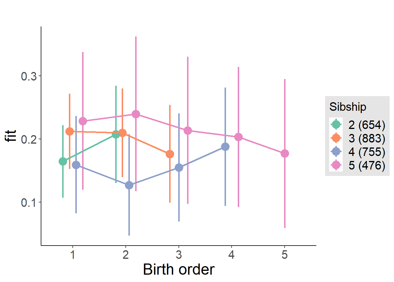
Model Comparison
###### Model 1 - Model 2
anova(m1_covariates_only, m2_birthorder_linear, m3_birthorder_nonlinear, m4_interaction)## refitting model(s) with ML (instead of REML)| Df | AIC | BIC | logLik | deviance | Chisq | Chi Df | Pr(>Chisq) |
|---|---|---|---|---|---|---|---|
| 10 | 2663 | 2722 | -1322 | 2643 | NA | NA | NA |
| 11 | 2665 | 2730 | -1321 | 2643 | 0.1642 | 1 | 0.6853 |
| 14 | 2669 | 2752 | -1321 | 2641 | 1.786 | 3 | 0.618 |
| 20 | 2676 | 2795 | -1318 | 2636 | 4.918 | 6 | 0.5544 |
Compare birth order specifications
library(coefplot)
multiplot(outcome_naive_m1, outcome_preg_m1, outcome_uterus_m1, outcome_parental_m1, dodgeHeight = 0.6,
intercept = FALSE)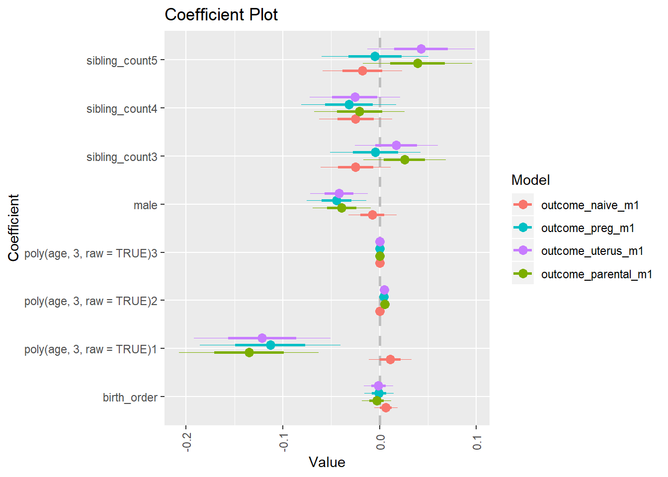
Category_Unpaid family worker
birthorder <- birthorder %>% mutate(outcome = `Category_Unpaid family worker`)
model = lmer(outcome ~ birth_order + poly(age, 3, raw = TRUE) + male + sibling_count + (1 | mother_pidlink),
data = birthorder)
compare_birthorder_specs(model)Naive birth order
outcome_naive_m1 <- update(m2_birthorder_linear, data = birthorder %>%
mutate(sibling_count = sibling_count_naive_factor,
birth_order_nonlinear = birthorder_naive_factor,
birth_order = birthorder_naive,
count_birth_order = count_birthorder_naive) %>%
filter(sibling_count != "1"))
compare_models_markdown(outcome_naive_m1)Basic Model
Model Summary
m1_covariates_only <- update(m2_birthorder_linear, formula = . ~ . - birth_order)
tidy(m1_covariates_only, conf.int = T, conf.level = 0.995)| effect | group | term | estimate | std.error | statistic | df | p.value | conf.low | conf.high |
|---|---|---|---|---|---|---|---|---|---|
| fixed | NA | (Intercept) | 1.074 | 0.08521 | 12.6 | 4365 | 8.547e-36 | 0.8347 | 1.313 |
| fixed | NA | poly(age, 3, raw = TRUE)1 | -0.07204 | 0.007602 | -9.476 | 4228 | 4.288e-21 | -0.09338 | -0.0507 |
| fixed | NA | poly(age, 3, raw = TRUE)2 | 0.001664 | 0.0002111 | 7.88 | 4069 | 4.185e-15 | 0.001071 | 0.002256 |
| fixed | NA | poly(age, 3, raw = TRUE)3 | -0.00001203 | 0.000001847 | -6.516 | 3928 | 0.00000000008141 | -0.00001722 | -0.000006849 |
| fixed | NA | male | -0.06956 | 0.008628 | -8.062 | 4736 | 9.418e-16 | -0.09378 | -0.04534 |
| fixed | NA | sibling_count3 | 0.01396 | 0.01249 | 1.117 | 3161 | 0.2639 | -0.02111 | 0.04903 |
| fixed | NA | sibling_count4 | 0.01928 | 0.01264 | 1.526 | 2926 | 0.1272 | -0.01619 | 0.05474 |
| fixed | NA | sibling_count5 | 0.02569 | 0.01319 | 1.948 | 2681 | 0.05157 | -0.01134 | 0.06271 |
| ran_pars | mother_pidlink | sd__(Intercept) | 0.1067 | NA | NA | NA | NA | NA | NA |
| ran_pars | Residual | sd__Observation | 0.2786 | NA | NA | NA | NA | NA | NA |
Coefficient Plot
plot(allEffects(m1_covariates_only, confidence.level = 0.995))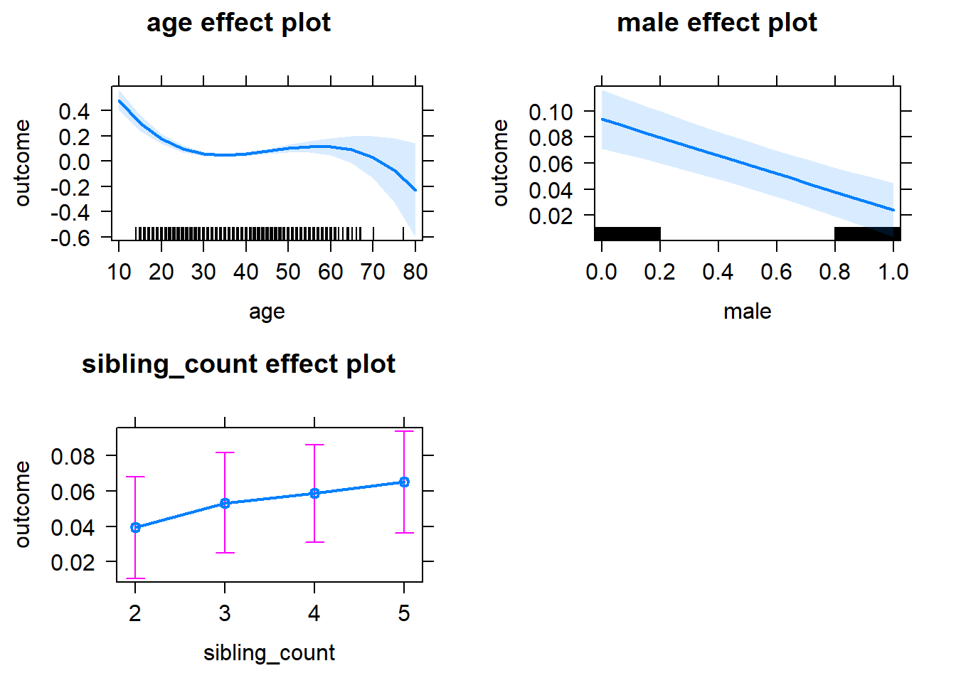
Add Birth Order Linear
Model Summary
tidy(m2_birthorder_linear, conf.int = T, conf.level = 0.995)| effect | group | term | estimate | std.error | statistic | df | p.value | conf.low | conf.high |
|---|---|---|---|---|---|---|---|---|---|
| fixed | NA | (Intercept) | 1.076 | 0.08512 | 12.65 | 4366 | 5.042e-36 | 0.8375 | 1.315 |
| fixed | NA | birth_order | 0.01404 | 0.00422 | 3.327 | 4059 | 0.0008856 | 0.002195 | 0.02589 |
| fixed | NA | poly(age, 3, raw = TRUE)1 | -0.07413 | 0.00762 | -9.728 | 4230 | 3.898e-22 | -0.09552 | -0.05274 |
| fixed | NA | poly(age, 3, raw = TRUE)2 | 0.001717 | 0.0002115 | 8.116 | 4060 | 6.323e-16 | 0.001123 | 0.00231 |
| fixed | NA | poly(age, 3, raw = TRUE)3 | -0.00001239 | 0.000001848 | -6.705 | 3920 | 0.00000000002296 | -0.00001758 | -0.000007204 |
| fixed | NA | male | -0.06942 | 0.008619 | -8.055 | 4735 | 9.991e-16 | -0.09362 | -0.04523 |
| fixed | NA | sibling_count3 | 0.00864 | 0.01258 | 0.6867 | 3262 | 0.4923 | -0.02668 | 0.04396 |
| fixed | NA | sibling_count4 | 0.008 | 0.01307 | 0.6121 | 3318 | 0.5405 | -0.02868 | 0.04468 |
| fixed | NA | sibling_count5 | 0.007656 | 0.01425 | 0.5374 | 3461 | 0.591 | -0.03233 | 0.04765 |
| ran_pars | mother_pidlink | sd__(Intercept) | 0.1065 | NA | NA | NA | NA | NA | NA |
| ran_pars | Residual | sd__Observation | 0.2783 | NA | NA | NA | NA | NA | NA |
Coefficient Plot
plot_birthorder2(m2_birthorder_linear, separate = FALSE)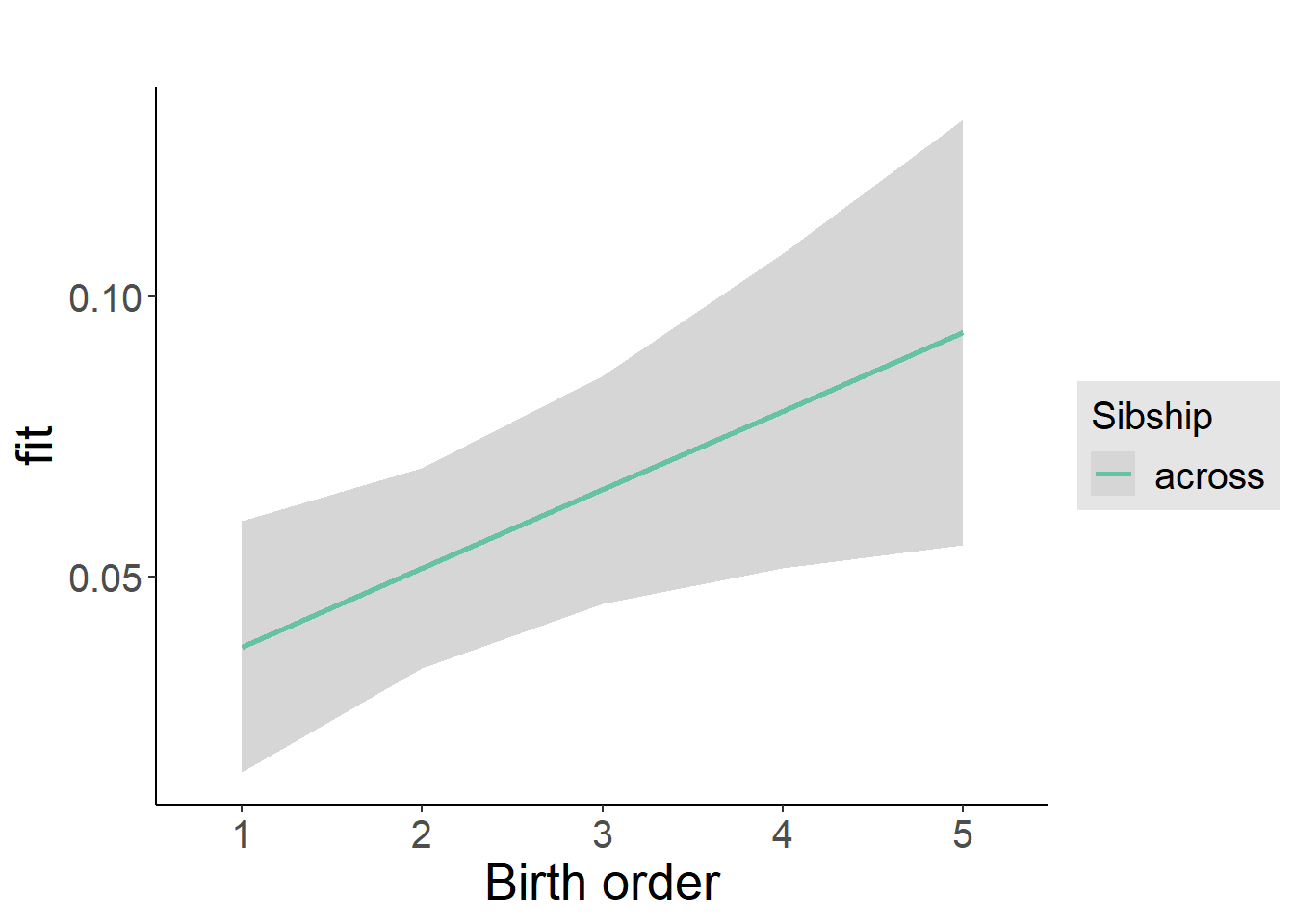
Add Birth Order Factor
Model Summary
m3_birthorder_nonlinear = update(m1_covariates_only, formula = . ~ . + birth_order_nonlinear)
tidy(m3_birthorder_nonlinear, conf.int = T, conf.level = 0.995)| effect | group | term | estimate | std.error | statistic | df | p.value | conf.low | conf.high |
|---|---|---|---|---|---|---|---|---|---|
| fixed | NA | (Intercept) | 1.09 | 0.08538 | 12.77 | 4371 | 1.082e-36 | 0.8506 | 1.33 |
| fixed | NA | poly(age, 3, raw = TRUE)1 | -0.07412 | 0.007624 | -9.723 | 4223 | 4.11e-22 | -0.09553 | -0.05272 |
| fixed | NA | poly(age, 3, raw = TRUE)2 | 0.001715 | 0.0002117 | 8.105 | 4048 | 6.948e-16 | 0.001121 | 0.00231 |
| fixed | NA | poly(age, 3, raw = TRUE)3 | -0.00001237 | 0.00000185 | -6.687 | 3899 | 0.00000000002607 | -0.00001756 | -0.000007177 |
| fixed | NA | male | -0.06943 | 0.008624 | -8.051 | 4732 | 1.031e-15 | -0.09364 | -0.04523 |
| fixed | NA | sibling_count3 | 0.007621 | 0.01279 | 0.5957 | 3435 | 0.5514 | -0.02829 | 0.04353 |
| fixed | NA | sibling_count4 | 0.007502 | 0.01329 | 0.5644 | 3499 | 0.5725 | -0.02981 | 0.04481 |
| fixed | NA | sibling_count5 | 0.007968 | 0.01438 | 0.5541 | 3572 | 0.5796 | -0.0324 | 0.04834 |
| fixed | NA | birth_order_nonlinear2 | 0.01536 | 0.01018 | 1.509 | 3961 | 0.1313 | -0.01321 | 0.04393 |
| fixed | NA | birth_order_nonlinear3 | 0.0327 | 0.01295 | 2.526 | 3881 | 0.01157 | -0.003638 | 0.06905 |
| fixed | NA | birth_order_nonlinear4 | 0.04024 | 0.01681 | 2.394 | 3834 | 0.01672 | -0.006946 | 0.08743 |
| fixed | NA | birth_order_nonlinear5 | 0.0522 | 0.02428 | 2.149 | 3849 | 0.03166 | -0.01597 | 0.1204 |
| ran_pars | mother_pidlink | sd__(Intercept) | 0.1063 | NA | NA | NA | NA | NA | NA |
| ran_pars | Residual | sd__Observation | 0.2785 | NA | NA | NA | NA | NA | NA |
Coefficient Plot
plot_birthorder(m3_birthorder_nonlinear, separate = FALSE)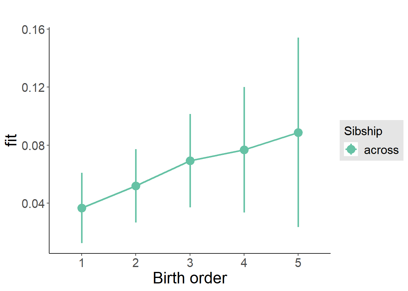
Add Interaction
Model Summary
m4_interaction = update(m3_birthorder_nonlinear, formula = . ~ . - birth_order_nonlinear - sibling_count + count_birth_order)
tidy(m4_interaction, conf.int = T, conf.level = 0.995)| effect | group | term | estimate | std.error | statistic | df | p.value | conf.low | conf.high |
|---|---|---|---|---|---|---|---|---|---|
| fixed | NA | (Intercept) | 1.098 | 0.08548 | 12.85 | 4377 | 4.03e-37 | 0.8584 | 1.338 |
| fixed | NA | poly(age, 3, raw = TRUE)1 | -0.07481 | 0.007627 | -9.809 | 4219 | 1.794e-22 | -0.09622 | -0.0534 |
| fixed | NA | poly(age, 3, raw = TRUE)2 | 0.00173 | 0.0002117 | 8.172 | 4043 | 4.012e-16 | 0.001136 | 0.002324 |
| fixed | NA | poly(age, 3, raw = TRUE)3 | -0.00001245 | 0.00000185 | -6.731 | 3894 | 0.00000000001927 | -0.00001764 | -0.000007259 |
| fixed | NA | male | -0.06975 | 0.008626 | -8.086 | 4726 | 7.789e-16 | -0.09396 | -0.04553 |
| fixed | NA | count_birth_order2/2 | 0.0182 | 0.01729 | 1.053 | 3901 | 0.2926 | -0.03033 | 0.06673 |
| fixed | NA | count_birth_order1/3 | 0.002468 | 0.01674 | 0.1475 | 4790 | 0.8828 | -0.04451 | 0.04945 |
| fixed | NA | count_birth_order2/3 | 0.01367 | 0.01856 | 0.7364 | 4803 | 0.4615 | -0.03843 | 0.06577 |
| fixed | NA | count_birth_order3/3 | 0.06707 | 0.02042 | 3.284 | 4806 | 0.00103 | 0.009745 | 0.1244 |
| fixed | NA | count_birth_order1/4 | 0.01324 | 0.01835 | 0.7216 | 4804 | 0.4706 | -0.03826 | 0.06474 |
| fixed | NA | count_birth_order2/4 | 0.01965 | 0.01968 | 0.9983 | 4806 | 0.3182 | -0.03559 | 0.07489 |
| fixed | NA | count_birth_order3/4 | 0.02922 | 0.02099 | 1.392 | 4804 | 0.164 | -0.02971 | 0.08815 |
| fixed | NA | count_birth_order4/4 | 0.0618 | 0.02233 | 2.767 | 4802 | 0.005679 | -0.0008934 | 0.1245 |
| fixed | NA | count_birth_order1/5 | 0.01713 | 0.02083 | 0.8224 | 4804 | 0.4109 | -0.04134 | 0.0756 |
| fixed | NA | count_birth_order2/5 | 0.04536 | 0.02211 | 2.051 | 4800 | 0.04028 | -0.01671 | 0.1074 |
| fixed | NA | count_birth_order3/5 | 0.02152 | 0.02328 | 0.9247 | 4793 | 0.3552 | -0.04381 | 0.08686 |
| fixed | NA | count_birth_order4/5 | 0.03329 | 0.02448 | 1.36 | 4768 | 0.174 | -0.03543 | 0.102 |
| fixed | NA | count_birth_order5/5 | 0.06105 | 0.0245 | 2.492 | 4787 | 0.01273 | -0.007715 | 0.1298 |
| ran_pars | mother_pidlink | sd__(Intercept) | 0.1059 | NA | NA | NA | NA | NA | NA |
| ran_pars | Residual | sd__Observation | 0.2786 | NA | NA | NA | NA | NA | NA |
Coefficient Plot
plot_birthorder(m4_interaction)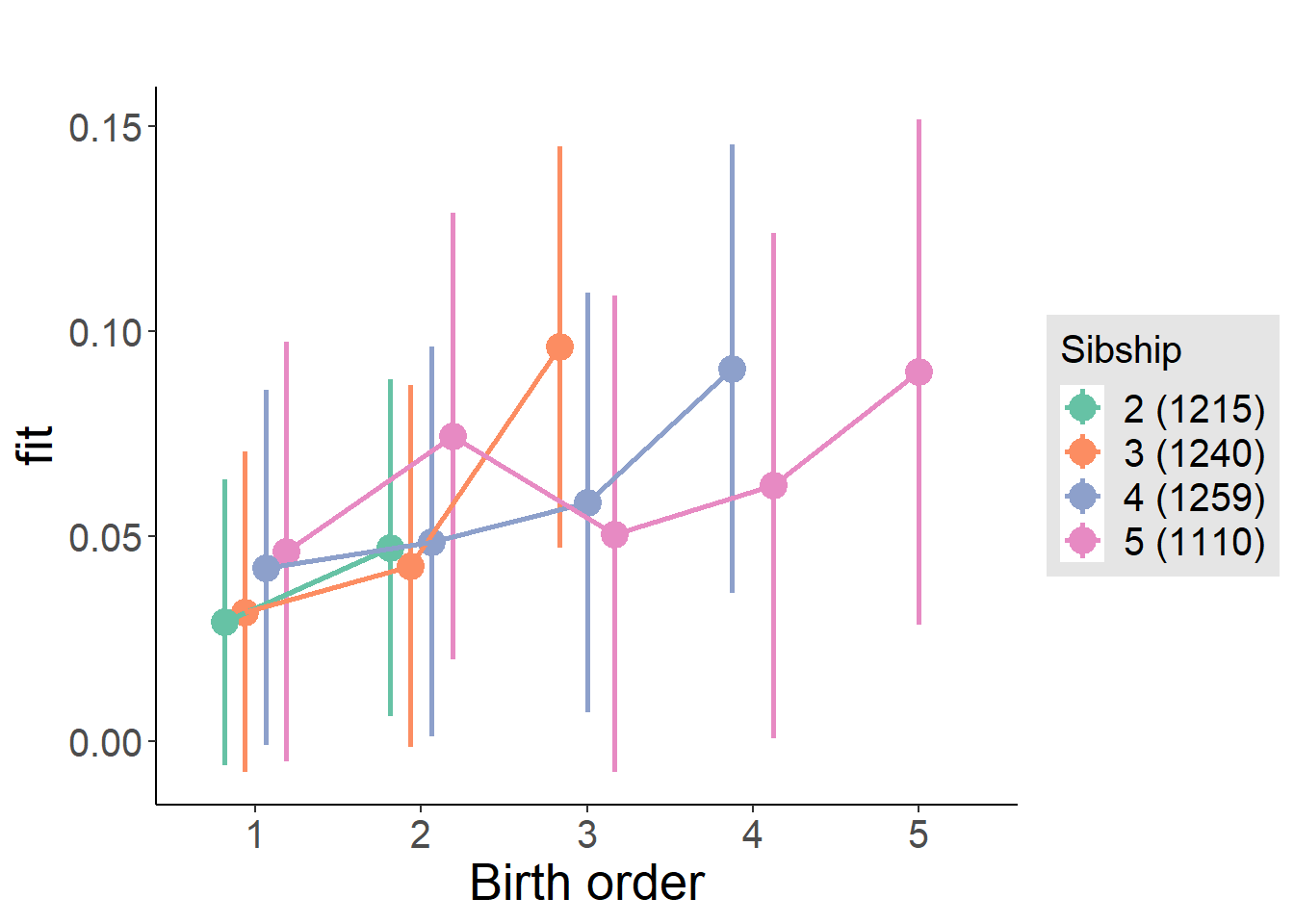
Model Comparison
###### Model 1 - Model 2
anova(m1_covariates_only, m2_birthorder_linear, m3_birthorder_nonlinear, m4_interaction)## refitting model(s) with ML (instead of REML)| Df | AIC | BIC | logLik | deviance | Chisq | Chi Df | Pr(>Chisq) |
|---|---|---|---|---|---|---|---|
| 10 | 2000 | 2065 | -990.1 | 1980 | NA | NA | NA |
| 11 | 1991 | 2062 | -984.6 | 1969 | 11.08 | 1 | 0.0008739 |
| 14 | 1997 | 2088 | -984.5 | 1969 | 0.2297 | 3 | 0.9727 |
| 20 | 2002 | 2131 | -980.8 | 1962 | 7.365 | 6 | 0.2884 |
Maternal birth order
outcome_uterus_m1 <- update(m2_birthorder_linear, data = birthorder %>%
mutate(sibling_count = sibling_count_uterus_alive_factor,
birth_order_nonlinear = birthorder_uterus_alive_factor,
birth_order = birthorder_uterus_alive,
count_birth_order = count_birthorder_uterus_alive) %>%
filter(sibling_count != "1"))
compare_models_markdown(outcome_uterus_m1)Basic Model
Model Summary
m1_covariates_only <- update(m2_birthorder_linear, formula = . ~ . - birth_order)
tidy(m1_covariates_only, conf.int = T, conf.level = 0.995)| effect | group | term | estimate | std.error | statistic | df | p.value | conf.low | conf.high |
|---|---|---|---|---|---|---|---|---|---|
| fixed | NA | (Intercept) | 2.811 | 0.2353 | 11.95 | 2746 | 4.014e-32 | 2.151 | 3.472 |
| fixed | NA | poly(age, 3, raw = TRUE)1 | -0.2645 | 0.02606 | -10.15 | 2746 | 8.764e-24 | -0.3377 | -0.1914 |
| fixed | NA | poly(age, 3, raw = TRUE)2 | 0.008156 | 0.0009243 | 8.824 | 2744 | 1.922e-18 | 0.005562 | 0.01075 |
| fixed | NA | poly(age, 3, raw = TRUE)3 | -0.00008159 | 0.0000105 | -7.772 | 2742 | 1.084e-14 | -0.0001111 | -0.00005212 |
| fixed | NA | male | -0.02304 | 0.01104 | -2.087 | 2732 | 0.03696 | -0.05402 | 0.007945 |
| fixed | NA | sibling_count3 | 0.02455 | 0.01542 | 1.592 | 1812 | 0.1116 | -0.01874 | 0.06783 |
| fixed | NA | sibling_count4 | 0.04627 | 0.01599 | 2.895 | 1588 | 0.003847 | 0.001401 | 0.09114 |
| fixed | NA | sibling_count5 | 0.0495 | 0.01776 | 2.787 | 1293 | 0.005402 | -0.0003603 | 0.09936 |
| ran_pars | mother_pidlink | sd__(Intercept) | 0.08741 | NA | NA | NA | NA | NA | NA |
| ran_pars | Residual | sd__Observation | 0.273 | NA | NA | NA | NA | NA | NA |
Coefficient Plot
plot(allEffects(m1_covariates_only, confidence.level = 0.995))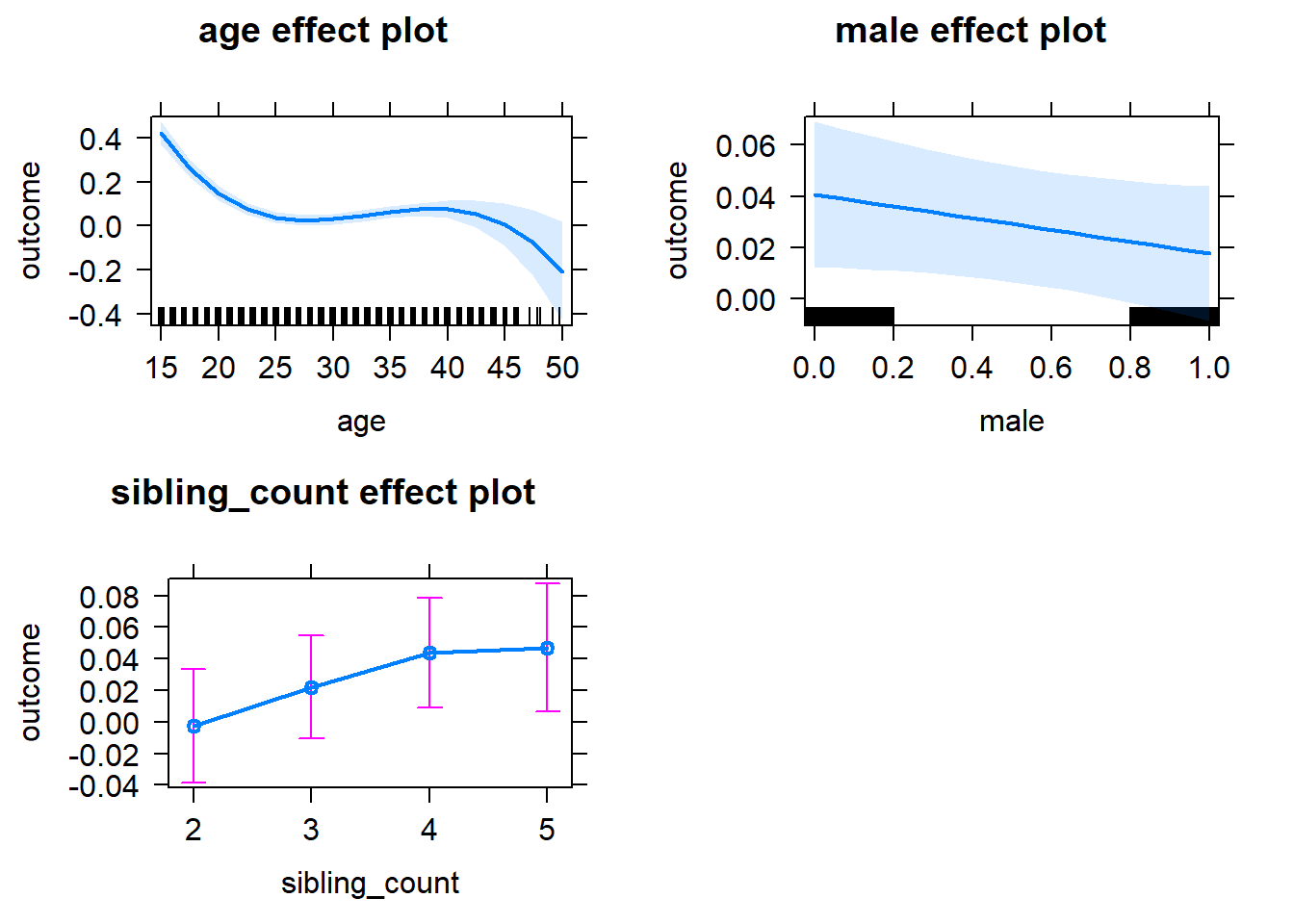
Add Birth Order Linear
Model Summary
tidy(m2_birthorder_linear, conf.int = T, conf.level = 0.995)| effect | group | term | estimate | std.error | statistic | df | p.value | conf.low | conf.high |
|---|---|---|---|---|---|---|---|---|---|
| fixed | NA | (Intercept) | 2.806 | 0.2352 | 11.93 | 2746 | 4.986e-32 | 2.146 | 3.466 |
| fixed | NA | birth_order | 0.01008 | 0.005552 | 1.816 | 2492 | 0.06947 | -0.005501 | 0.02567 |
| fixed | NA | poly(age, 3, raw = TRUE)1 | -0.2651 | 0.02606 | -10.18 | 2745 | 6.767e-24 | -0.3383 | -0.192 |
| fixed | NA | poly(age, 3, raw = TRUE)2 | 0.008161 | 0.0009239 | 8.833 | 2744 | 1.788e-18 | 0.005567 | 0.01075 |
| fixed | NA | poly(age, 3, raw = TRUE)3 | -0.00008138 | 0.00001049 | -7.755 | 2742 | 1.24e-14 | -0.0001108 | -0.00005192 |
| fixed | NA | male | -0.02304 | 0.01103 | -2.088 | 2730 | 0.03685 | -0.05401 | 0.007928 |
| fixed | NA | sibling_count3 | 0.01969 | 0.01565 | 1.258 | 1855 | 0.2085 | -0.02424 | 0.06363 |
| fixed | NA | sibling_count4 | 0.03593 | 0.01697 | 2.117 | 1751 | 0.03443 | -0.01172 | 0.08358 |
| fixed | NA | sibling_count5 | 0.03213 | 0.02019 | 1.591 | 1680 | 0.1118 | -0.02456 | 0.08881 |
| ran_pars | mother_pidlink | sd__(Intercept) | 0.08833 | NA | NA | NA | NA | NA | NA |
| ran_pars | Residual | sd__Observation | 0.2726 | NA | NA | NA | NA | NA | NA |
Coefficient Plot
plot_birthorder2(m2_birthorder_linear, separate = FALSE)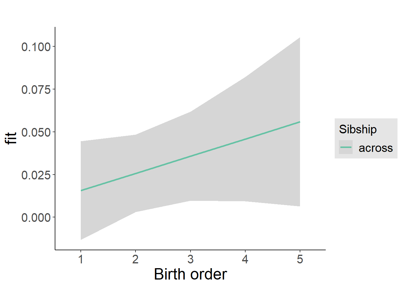
Add Birth Order Factor
Model Summary
m3_birthorder_nonlinear = update(m1_covariates_only, formula = . ~ . + birth_order_nonlinear)
tidy(m3_birthorder_nonlinear, conf.int = T, conf.level = 0.995)| effect | group | term | estimate | std.error | statistic | df | p.value | conf.low | conf.high |
|---|---|---|---|---|---|---|---|---|---|
| fixed | NA | (Intercept) | 2.805 | 0.2357 | 11.9 | 2741 | 7.027e-32 | 2.143 | 3.467 |
| fixed | NA | poly(age, 3, raw = TRUE)1 | -0.264 | 0.0261 | -10.11 | 2741 | 1.24e-23 | -0.3373 | -0.1907 |
| fixed | NA | poly(age, 3, raw = TRUE)2 | 0.00812 | 0.0009256 | 8.773 | 2740 | 3.005e-18 | 0.005522 | 0.01072 |
| fixed | NA | poly(age, 3, raw = TRUE)3 | -0.00008093 | 0.00001051 | -7.699 | 2739 | 1.906e-14 | -0.0001104 | -0.00005142 |
| fixed | NA | male | -0.02285 | 0.01104 | -2.07 | 2729 | 0.03855 | -0.05384 | 0.008138 |
| fixed | NA | sibling_count3 | 0.01713 | 0.01589 | 1.078 | 1944 | 0.2812 | -0.02748 | 0.06173 |
| fixed | NA | sibling_count4 | 0.03296 | 0.0172 | 1.917 | 1831 | 0.05541 | -0.01531 | 0.08123 |
| fixed | NA | sibling_count5 | 0.03575 | 0.02045 | 1.748 | 1735 | 0.0806 | -0.02165 | 0.09314 |
| fixed | NA | birth_order_nonlinear2 | 0.01559 | 0.01327 | 1.175 | 2071 | 0.2401 | -0.02166 | 0.05284 |
| fixed | NA | birth_order_nonlinear3 | 0.03148 | 0.0162 | 1.943 | 2189 | 0.05211 | -0.01399 | 0.07696 |
| fixed | NA | birth_order_nonlinear4 | 0.03481 | 0.02152 | 1.618 | 2311 | 0.1058 | -0.02559 | 0.0952 |
| fixed | NA | birth_order_nonlinear5 | 0.00941 | 0.03305 | 0.2847 | 2219 | 0.7759 | -0.08337 | 0.1022 |
| ran_pars | mother_pidlink | sd__(Intercept) | 0.08756 | NA | NA | NA | NA | NA | NA |
| ran_pars | Residual | sd__Observation | 0.2729 | NA | NA | NA | NA | NA | NA |
Coefficient Plot
plot_birthorder(m3_birthorder_nonlinear, separate = FALSE)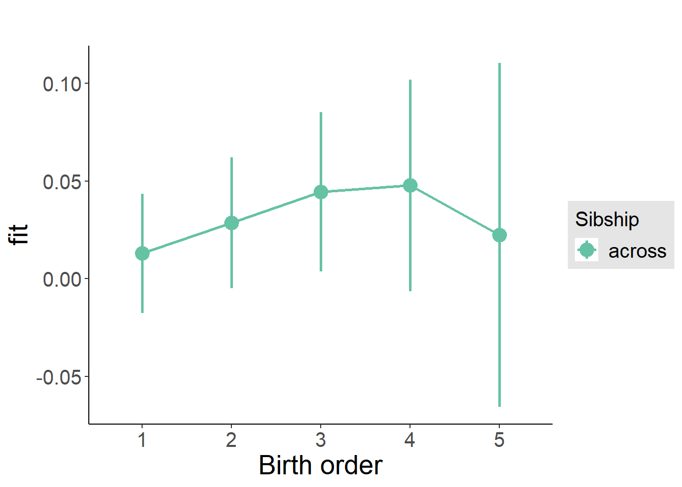
Add Interaction
Model Summary
m4_interaction = update(m3_birthorder_nonlinear, formula = . ~ . - birth_order_nonlinear - sibling_count + count_birth_order)
tidy(m4_interaction, conf.int = T, conf.level = 0.995)| effect | group | term | estimate | std.error | statistic | df | p.value | conf.low | conf.high |
|---|---|---|---|---|---|---|---|---|---|
| fixed | NA | (Intercept) | 2.795 | 0.2357 | 11.86 | 2736 | 1.163e-31 | 2.134 | 3.457 |
| fixed | NA | poly(age, 3, raw = TRUE)1 | -0.2627 | 0.02611 | -10.06 | 2736 | 2.076e-23 | -0.3359 | -0.1894 |
| fixed | NA | poly(age, 3, raw = TRUE)2 | 0.00808 | 0.0009258 | 8.727 | 2735 | 4.462e-18 | 0.005481 | 0.01068 |
| fixed | NA | poly(age, 3, raw = TRUE)3 | -0.00008057 | 0.00001052 | -7.661 | 2734 | 2.535e-14 | -0.0001101 | -0.00005105 |
| fixed | NA | male | -0.02213 | 0.01105 | -2.003 | 2722 | 0.04532 | -0.05314 | 0.008888 |
| fixed | NA | count_birth_order2/2 | 0.003644 | 0.02406 | 0.1514 | 2146 | 0.8796 | -0.0639 | 0.07119 |
| fixed | NA | count_birth_order1/3 | -0.001973 | 0.0203 | -0.09719 | 2746 | 0.9226 | -0.05896 | 0.05501 |
| fixed | NA | count_birth_order2/3 | 0.03066 | 0.02255 | 1.36 | 2750 | 0.174 | -0.03264 | 0.09396 |
| fixed | NA | count_birth_order3/3 | 0.07164 | 0.0244 | 2.936 | 2745 | 0.003355 | 0.003141 | 0.1401 |
| fixed | NA | count_birth_order1/4 | 0.04786 | 0.02339 | 2.046 | 2749 | 0.04084 | -0.0178 | 0.1135 |
| fixed | NA | count_birth_order2/4 | 0.0325 | 0.02457 | 1.323 | 2748 | 0.186 | -0.03648 | 0.1015 |
| fixed | NA | count_birth_order3/4 | 0.0417 | 0.02577 | 1.618 | 2738 | 0.1058 | -0.03064 | 0.114 |
| fixed | NA | count_birth_order4/4 | 0.07336 | 0.0273 | 2.687 | 2737 | 0.007262 | -0.003289 | 0.15 |
| fixed | NA | count_birth_order1/5 | 0.0305 | 0.03076 | 0.9913 | 2749 | 0.3216 | -0.05586 | 0.1168 |
| fixed | NA | count_birth_order2/5 | 0.08913 | 0.03342 | 2.667 | 2726 | 0.007694 | -0.004673 | 0.1829 |
| fixed | NA | count_birth_order3/5 | 0.04419 | 0.03127 | 1.413 | 2728 | 0.1578 | -0.0436 | 0.132 |
| fixed | NA | count_birth_order4/5 | 0.05387 | 0.03039 | 1.773 | 2723 | 0.07637 | -0.03143 | 0.1392 |
| fixed | NA | count_birth_order5/5 | 0.04117 | 0.03186 | 1.292 | 2715 | 0.1964 | -0.04826 | 0.1306 |
| ran_pars | mother_pidlink | sd__(Intercept) | 0.08807 | NA | NA | NA | NA | NA | NA |
| ran_pars | Residual | sd__Observation | 0.2727 | NA | NA | NA | NA | NA | NA |
Coefficient Plot
plot_birthorder(m4_interaction)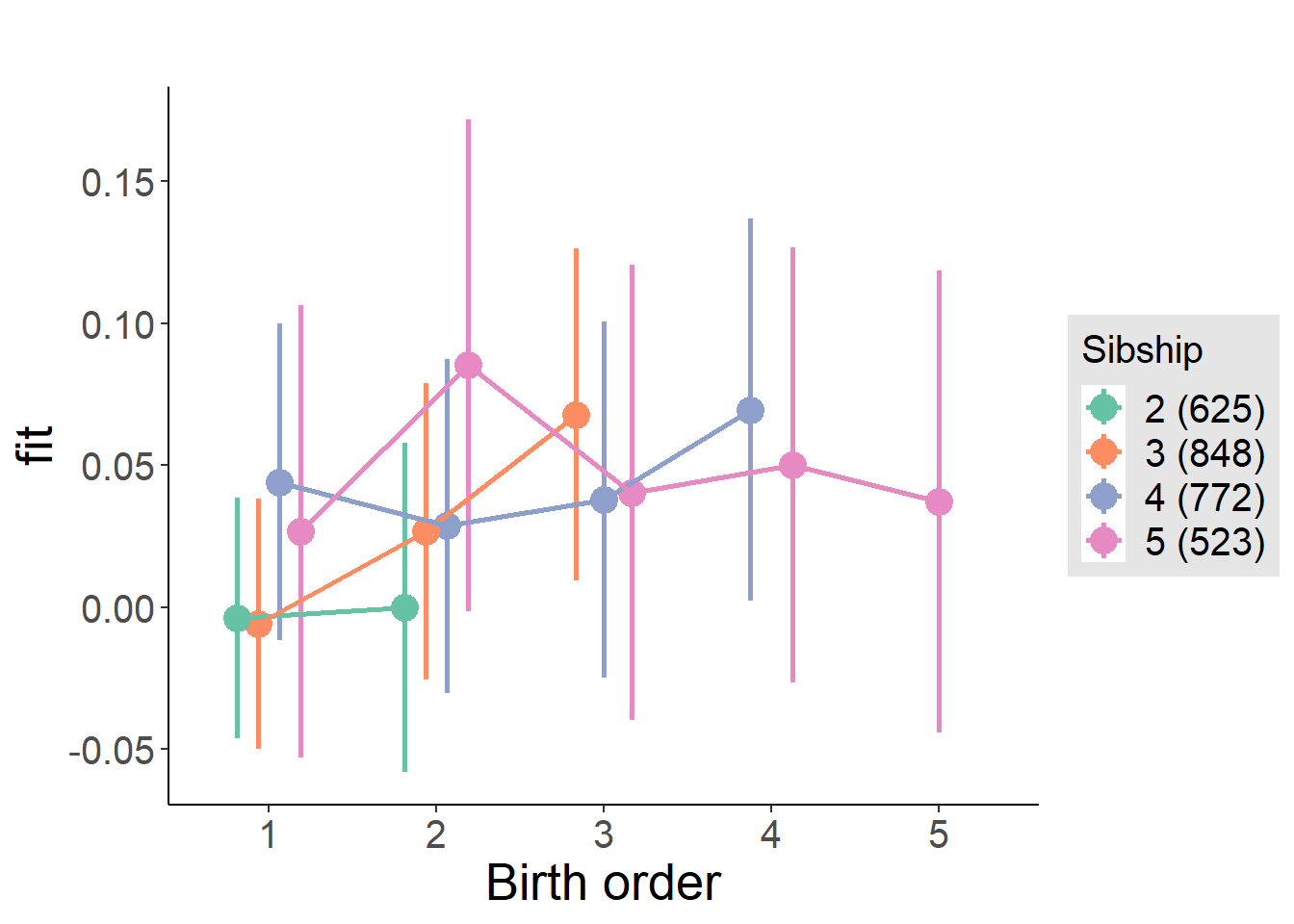
Model Comparison
###### Model 1 - Model 2
anova(m1_covariates_only, m2_birthorder_linear, m3_birthorder_nonlinear, m4_interaction)## refitting model(s) with ML (instead of REML)| Df | AIC | BIC | logLik | deviance | Chisq | Chi Df | Pr(>Chisq) |
|---|---|---|---|---|---|---|---|
| 10 | 943.3 | 1003 | -461.6 | 923.3 | NA | NA | NA |
| 11 | 942 | 1007 | -460 | 920 | 3.299 | 1 | 0.06933 |
| 14 | 946.1 | 1029 | -459.1 | 918.1 | 1.856 | 3 | 0.6028 |
| 20 | 949.7 | 1068 | -454.9 | 909.7 | 8.372 | 6 | 0.2121 |
Maternal pregnancy order
outcome_preg_m1 <- update(m2_birthorder_linear, data = birthorder %>%
mutate(sibling_count = sibling_count_uterus_preg_factor,
birth_order_nonlinear = birthorder_uterus_preg_factor,
birth_order = birthorder_uterus_preg,
count_birth_order = count_birthorder_uterus_preg
) %>%
filter(sibling_count != "1"))
compare_models_markdown(outcome_preg_m1)Basic Model
Model Summary
m1_covariates_only <- update(m2_birthorder_linear, formula = . ~ . - birth_order)
tidy(m1_covariates_only, conf.int = T, conf.level = 0.995)| effect | group | term | estimate | std.error | statistic | df | p.value | conf.low | conf.high |
|---|---|---|---|---|---|---|---|---|---|
| fixed | NA | (Intercept) | 2.879 | 0.2445 | 11.78 | 2518 | 3.354e-31 | 2.193 | 3.566 |
| fixed | NA | poly(age, 3, raw = TRUE)1 | -0.2724 | 0.0271 | -10.05 | 2517 | 2.452e-23 | -0.3485 | -0.1964 |
| fixed | NA | poly(age, 3, raw = TRUE)2 | 0.008458 | 0.0009611 | 8.8 | 2515 | 2.487e-18 | 0.00576 | 0.01116 |
| fixed | NA | poly(age, 3, raw = TRUE)3 | -0.000085 | 0.00001092 | -7.787 | 2512 | 9.972e-15 | -0.0001156 | -0.00005436 |
| fixed | NA | male | -0.0269 | 0.01158 | -2.323 | 2518 | 0.02024 | -0.05941 | 0.005602 |
| fixed | NA | sibling_count3 | 0.02317 | 0.0169 | 1.371 | 1777 | 0.1704 | -0.02426 | 0.0706 |
| fixed | NA | sibling_count4 | 0.03722 | 0.01709 | 2.178 | 1632 | 0.02953 | -0.01074 | 0.08519 |
| fixed | NA | sibling_count5 | 0.02973 | 0.018 | 1.651 | 1417 | 0.09889 | -0.0208 | 0.08026 |
| ran_pars | mother_pidlink | sd__(Intercept) | 0.07611 | NA | NA | NA | NA | NA | NA |
| ran_pars | Residual | sd__Observation | 0.2773 | NA | NA | NA | NA | NA | NA |
Coefficient Plot
plot(allEffects(m1_covariates_only, confidence.level = 0.995))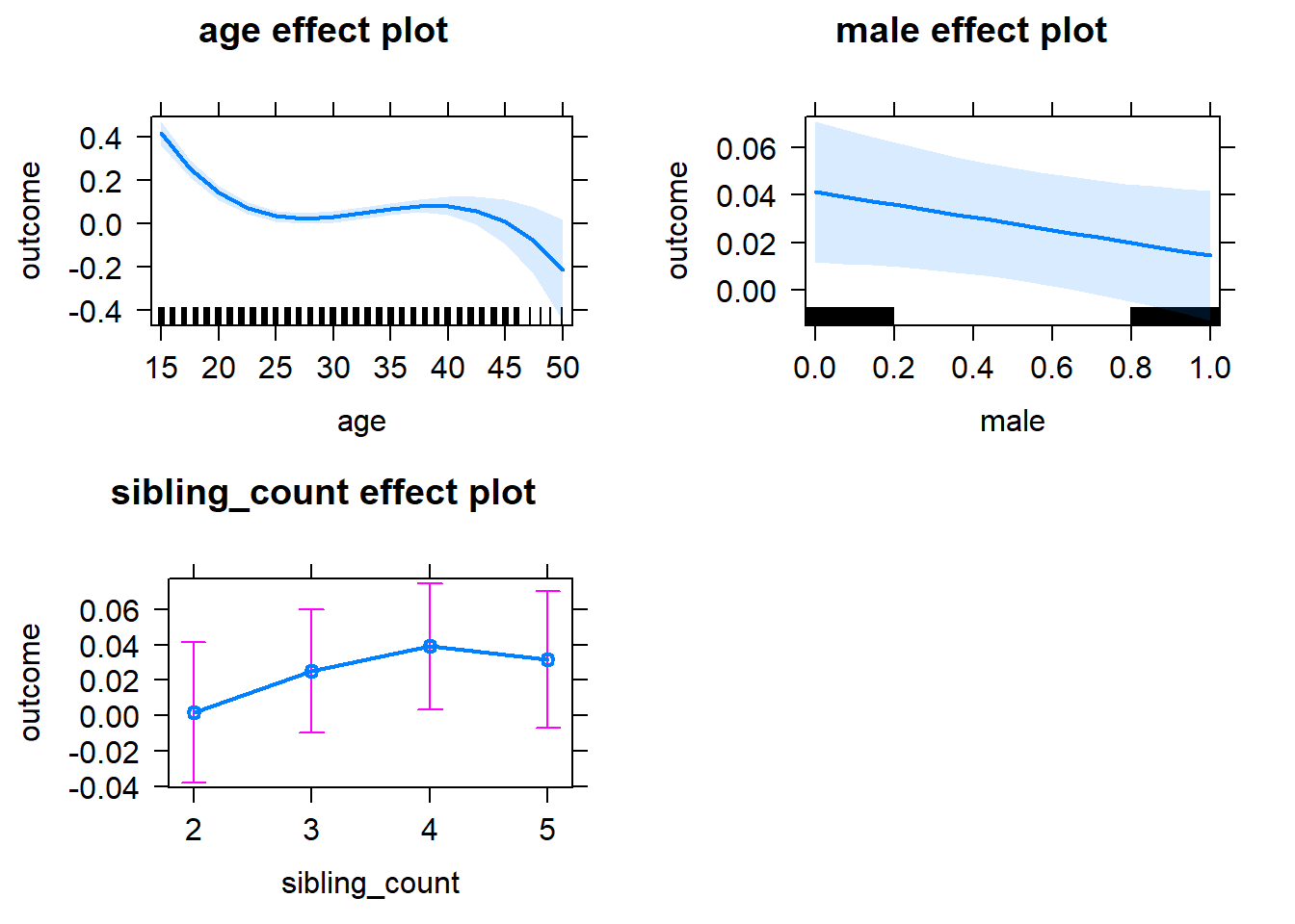
Add Birth Order Linear
Model Summary
tidy(m2_birthorder_linear, conf.int = T, conf.level = 0.995)| effect | group | term | estimate | std.error | statistic | df | p.value | conf.low | conf.high |
|---|---|---|---|---|---|---|---|---|---|
| fixed | NA | (Intercept) | 2.864 | 0.2443 | 11.72 | 2518 | 6.181e-31 | 2.178 | 3.55 |
| fixed | NA | birth_order | 0.01445 | 0.005651 | 2.558 | 2400 | 0.0106 | -0.00141 | 0.03032 |
| fixed | NA | poly(age, 3, raw = TRUE)1 | -0.2726 | 0.02707 | -10.07 | 2517 | 2.07e-23 | -0.3486 | -0.1966 |
| fixed | NA | poly(age, 3, raw = TRUE)2 | 0.008446 | 0.0009601 | 8.797 | 2515 | 2.553e-18 | 0.005751 | 0.01114 |
| fixed | NA | poly(age, 3, raw = TRUE)3 | -0.00008455 | 0.00001091 | -7.753 | 2513 | 1.298e-14 | -0.0001152 | -0.00005393 |
| fixed | NA | male | -0.02644 | 0.01157 | -2.286 | 2516 | 0.02236 | -0.05891 | 0.006033 |
| fixed | NA | sibling_count3 | 0.01605 | 0.01711 | 0.9378 | 1802 | 0.3485 | -0.03199 | 0.06408 |
| fixed | NA | sibling_count4 | 0.02332 | 0.01792 | 1.302 | 1737 | 0.1932 | -0.02698 | 0.07362 |
| fixed | NA | sibling_count5 | 0.006451 | 0.02017 | 0.3199 | 1709 | 0.7491 | -0.05016 | 0.06306 |
| ran_pars | mother_pidlink | sd__(Intercept) | 0.0769 | NA | NA | NA | NA | NA | NA |
| ran_pars | Residual | sd__Observation | 0.2767 | NA | NA | NA | NA | NA | NA |
Coefficient Plot
plot_birthorder2(m2_birthorder_linear, separate = FALSE)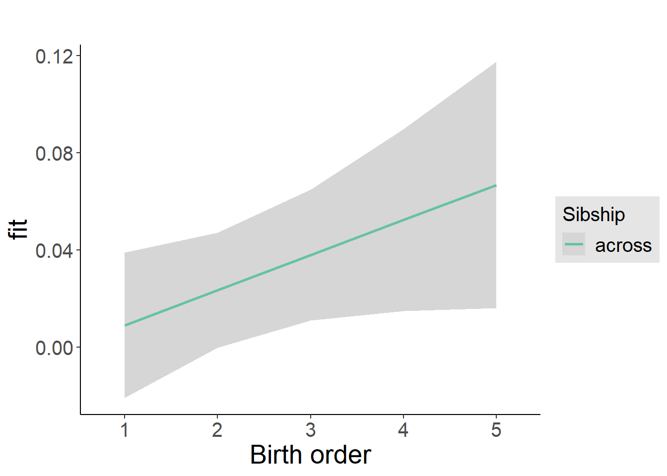
Add Birth Order Factor
Model Summary
m3_birthorder_nonlinear = update(m1_covariates_only, formula = . ~ . + birth_order_nonlinear)
tidy(m3_birthorder_nonlinear, conf.int = T, conf.level = 0.995)| effect | group | term | estimate | std.error | statistic | df | p.value | conf.low | conf.high |
|---|---|---|---|---|---|---|---|---|---|
| fixed | NA | (Intercept) | 2.848 | 0.2447 | 11.64 | 2511 | 1.563e-30 | 2.161 | 3.535 |
| fixed | NA | poly(age, 3, raw = TRUE)1 | -0.2693 | 0.02711 | -9.932 | 2511 | 7.882e-23 | -0.3454 | -0.1932 |
| fixed | NA | poly(age, 3, raw = TRUE)2 | 0.008331 | 0.0009615 | 8.665 | 2510 | 7.976e-18 | 0.005632 | 0.01103 |
| fixed | NA | poly(age, 3, raw = TRUE)3 | -0.00008329 | 0.00001092 | -7.628 | 2507 | 3.371e-14 | -0.0001139 | -0.00005264 |
| fixed | NA | male | -0.02615 | 0.01157 | -2.261 | 2513 | 0.02384 | -0.05861 | 0.006315 |
| fixed | NA | sibling_count3 | 0.01028 | 0.01736 | 0.5921 | 1869 | 0.5538 | -0.03845 | 0.059 |
| fixed | NA | sibling_count4 | 0.01685 | 0.01814 | 0.9293 | 1798 | 0.3528 | -0.03405 | 0.06776 |
| fixed | NA | sibling_count5 | 0.009426 | 0.02028 | 0.4647 | 1736 | 0.6422 | -0.04751 | 0.06636 |
| fixed | NA | birth_order_nonlinear2 | 0.01544 | 0.01386 | 1.114 | 1988 | 0.2656 | -0.02348 | 0.05436 |
| fixed | NA | birth_order_nonlinear3 | 0.05358 | 0.01708 | 3.137 | 2150 | 0.001727 | 0.005643 | 0.1015 |
| fixed | NA | birth_order_nonlinear4 | 0.05188 | 0.02237 | 2.319 | 2247 | 0.02049 | -0.01092 | 0.1147 |
| fixed | NA | birth_order_nonlinear5 | 0.007977 | 0.03201 | 0.2492 | 2152 | 0.8032 | -0.08187 | 0.09783 |
| ran_pars | mother_pidlink | sd__(Intercept) | 0.07712 | NA | NA | NA | NA | NA | NA |
| ran_pars | Residual | sd__Observation | 0.2765 | NA | NA | NA | NA | NA | NA |
Coefficient Plot
plot_birthorder(m3_birthorder_nonlinear, separate = FALSE)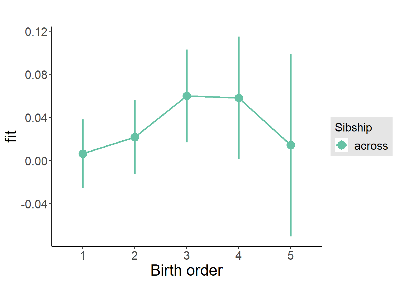
Add Interaction
Model Summary
m4_interaction = update(m3_birthorder_nonlinear, formula = . ~ . - birth_order_nonlinear - sibling_count + count_birth_order)
tidy(m4_interaction, conf.int = T, conf.level = 0.995)| effect | group | term | estimate | std.error | statistic | df | p.value | conf.low | conf.high |
|---|---|---|---|---|---|---|---|---|---|
| fixed | NA | (Intercept) | 2.832 | 0.2445 | 11.58 | 2505 | 2.983e-30 | 2.146 | 3.518 |
| fixed | NA | poly(age, 3, raw = TRUE)1 | -0.2678 | 0.02709 | -9.885 | 2504 | 1.25e-22 | -0.3439 | -0.1918 |
| fixed | NA | poly(age, 3, raw = TRUE)2 | 0.008279 | 0.0009608 | 8.617 | 2502 | 1.202e-17 | 0.005582 | 0.01098 |
| fixed | NA | poly(age, 3, raw = TRUE)3 | -0.00008274 | 0.00001091 | -7.581 | 2500 | 4.794e-14 | -0.0001134 | -0.0000521 |
| fixed | NA | male | -0.02514 | 0.01157 | -2.172 | 2509 | 0.02992 | -0.05763 | 0.007345 |
| fixed | NA | count_birth_order2/2 | 0.02236 | 0.02659 | 0.8409 | 2100 | 0.4005 | -0.05228 | 0.097 |
| fixed | NA | count_birth_order1/3 | 0.001725 | 0.02247 | 0.0768 | 2519 | 0.9388 | -0.06134 | 0.06479 |
| fixed | NA | count_birth_order2/3 | 0.02104 | 0.02443 | 0.8611 | 2521 | 0.3892 | -0.04755 | 0.08963 |
| fixed | NA | count_birth_order3/3 | 0.09582 | 0.02688 | 3.564 | 2518 | 0.0003721 | 0.02035 | 0.1713 |
| fixed | NA | count_birth_order1/4 | 0.04831 | 0.02451 | 1.971 | 2519 | 0.0488 | -0.02048 | 0.1171 |
| fixed | NA | count_birth_order2/4 | 0.007382 | 0.02556 | 0.2888 | 2521 | 0.7728 | -0.06438 | 0.07914 |
| fixed | NA | count_birth_order3/4 | 0.05718 | 0.02795 | 2.046 | 2515 | 0.04087 | -0.02127 | 0.1356 |
| fixed | NA | count_birth_order4/4 | 0.07931 | 0.0298 | 2.661 | 2513 | 0.007831 | -0.00434 | 0.163 |
| fixed | NA | count_birth_order1/5 | -0.007822 | 0.02944 | -0.2657 | 2521 | 0.7905 | -0.09047 | 0.07482 |
| fixed | NA | count_birth_order2/5 | 0.07993 | 0.03056 | 2.615 | 2518 | 0.008965 | -0.005857 | 0.1657 |
| fixed | NA | count_birth_order3/5 | 0.04252 | 0.03109 | 1.368 | 2512 | 0.1715 | -0.04474 | 0.1298 |
| fixed | NA | count_birth_order4/5 | 0.0536 | 0.03156 | 1.699 | 2506 | 0.08949 | -0.03497 | 0.1422 |
| fixed | NA | count_birth_order5/5 | 0.0195 | 0.03179 | 0.6132 | 2500 | 0.5398 | -0.06975 | 0.1087 |
| ran_pars | mother_pidlink | sd__(Intercept) | 0.07481 | NA | NA | NA | NA | NA | NA |
| ran_pars | Residual | sd__Observation | 0.2767 | NA | NA | NA | NA | NA | NA |
Coefficient Plot
plot_birthorder(m4_interaction)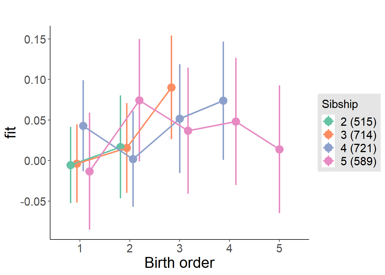
Model Comparison
###### Model 1 - Model 2
anova(m1_covariates_only, m2_birthorder_linear, m3_birthorder_nonlinear, m4_interaction)## refitting model(s) with ML (instead of REML)| Df | AIC | BIC | logLik | deviance | Chisq | Chi Df | Pr(>Chisq) |
|---|---|---|---|---|---|---|---|
| 10 | 883.9 | 942.3 | -432 | 863.9 | NA | NA | NA |
| 11 | 879.4 | 943.6 | -428.7 | 857.4 | 6.55 | 1 | 0.01049 |
| 14 | 879.4 | 961.1 | -425.7 | 851.4 | 6.01 | 3 | 0.1111 |
| 20 | 878.1 | 994.9 | -419.1 | 838.1 | 13.25 | 6 | 0.03924 |
Parental full sibling order
outcome_parental_m1 <- update(m2_birthorder_linear, data = birthorder %>%
mutate(sibling_count = sibling_count_genes_factor,
birth_order_nonlinear = birthorder_genes_factor,
birth_order = birthorder_genes,
count_birth_order = count_birthorder_genes
) %>%
filter(sibling_count != "1"))
compare_models_markdown(outcome_parental_m1)Basic Model
Model Summary
m1_covariates_only <- update(m2_birthorder_linear, formula = . ~ . - birth_order)
tidy(m1_covariates_only, conf.int = T, conf.level = 0.995)| effect | group | term | estimate | std.error | statistic | df | p.value | conf.low | conf.high |
|---|---|---|---|---|---|---|---|---|---|
| fixed | NA | (Intercept) | 2.754 | 0.2368 | 11.63 | 2746 | 1.523e-30 | 2.089 | 3.418 |
| fixed | NA | poly(age, 3, raw = TRUE)1 | -0.2578 | 0.0263 | -9.802 | 2746 | 2.563e-22 | -0.3317 | -0.184 |
| fixed | NA | poly(age, 3, raw = TRUE)2 | 0.007914 | 0.0009349 | 8.464 | 2745 | 4.127e-17 | 0.005289 | 0.01054 |
| fixed | NA | poly(age, 3, raw = TRUE)3 | -0.00007893 | 0.00001065 | -7.414 | 2743 | 1.621e-13 | -0.0001088 | -0.00004905 |
| fixed | NA | male | -0.02007 | 0.01099 | -1.826 | 2728 | 0.06797 | -0.05092 | 0.01078 |
| fixed | NA | sibling_count3 | 0.02623 | 0.01509 | 1.739 | 1864 | 0.08224 | -0.01612 | 0.06858 |
| fixed | NA | sibling_count4 | 0.04453 | 0.01586 | 2.808 | 1641 | 0.005037 | 0.00002278 | 0.08904 |
| fixed | NA | sibling_count5 | 0.05563 | 0.01811 | 3.072 | 1278 | 0.002175 | 0.00479 | 0.1065 |
| ran_pars | mother_pidlink | sd__(Intercept) | 0.09166 | NA | NA | NA | NA | NA | NA |
| ran_pars | Residual | sd__Observation | 0.2706 | NA | NA | NA | NA | NA | NA |
Coefficient Plot
plot(allEffects(m1_covariates_only, confidence.level = 0.995))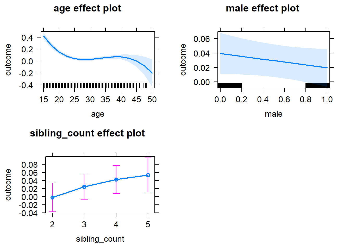
Add Birth Order Linear
Model Summary
tidy(m2_birthorder_linear, conf.int = T, conf.level = 0.995)| effect | group | term | estimate | std.error | statistic | df | p.value | conf.low | conf.high |
|---|---|---|---|---|---|---|---|---|---|
| fixed | NA | (Intercept) | 2.747 | 0.2367 | 11.61 | 2746 | 1.951e-30 | 2.083 | 3.411 |
| fixed | NA | birth_order | 0.01227 | 0.005592 | 2.194 | 2471 | 0.0283 | -0.003426 | 0.02797 |
| fixed | NA | poly(age, 3, raw = TRUE)1 | -0.2586 | 0.02629 | -9.835 | 2745 | 1.854e-22 | -0.3324 | -0.1848 |
| fixed | NA | poly(age, 3, raw = TRUE)2 | 0.007921 | 0.0009343 | 8.477 | 2744 | 3.708e-17 | 0.005298 | 0.01054 |
| fixed | NA | poly(age, 3, raw = TRUE)3 | -0.0000787 | 0.00001064 | -7.397 | 2743 | 1.843e-13 | -0.0001086 | -0.00004884 |
| fixed | NA | male | -0.01995 | 0.01098 | -1.817 | 2726 | 0.06939 | -0.05078 | 0.01088 |
| fixed | NA | sibling_count3 | 0.02025 | 0.01533 | 1.321 | 1903 | 0.1865 | -0.02277 | 0.06328 |
| fixed | NA | sibling_count4 | 0.03207 | 0.01684 | 1.905 | 1808 | 0.05696 | -0.01519 | 0.07934 |
| fixed | NA | sibling_count5 | 0.03518 | 0.02037 | 1.727 | 1621 | 0.08438 | -0.02201 | 0.09238 |
| ran_pars | mother_pidlink | sd__(Intercept) | 0.09243 | NA | NA | NA | NA | NA | NA |
| ran_pars | Residual | sd__Observation | 0.2701 | NA | NA | NA | NA | NA | NA |
Coefficient Plot
plot_birthorder2(m2_birthorder_linear, separate = FALSE)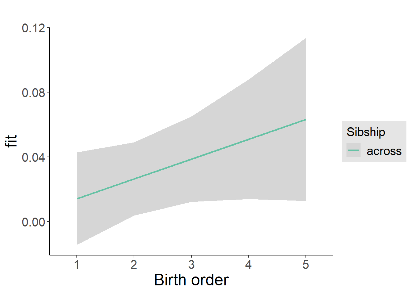
Add Birth Order Factor
Model Summary
m3_birthorder_nonlinear = update(m1_covariates_only, formula = . ~ . + birth_order_nonlinear)
tidy(m3_birthorder_nonlinear, conf.int = T, conf.level = 0.995)| effect | group | term | estimate | std.error | statistic | df | p.value | conf.low | conf.high |
|---|---|---|---|---|---|---|---|---|---|
| fixed | NA | (Intercept) | 2.753 | 0.2372 | 11.61 | 2740 | 1.865e-30 | 2.088 | 3.419 |
| fixed | NA | poly(age, 3, raw = TRUE)1 | -0.2581 | 0.02634 | -9.801 | 2741 | 2.583e-22 | -0.3321 | -0.1842 |
| fixed | NA | poly(age, 3, raw = TRUE)2 | 0.007904 | 0.0009361 | 8.444 | 2740 | 4.912e-17 | 0.005276 | 0.01053 |
| fixed | NA | poly(age, 3, raw = TRUE)3 | -0.00007851 | 0.00001066 | -7.366 | 2739 | 2.311e-13 | -0.0001084 | -0.00004859 |
| fixed | NA | male | -0.01989 | 0.011 | -1.809 | 2726 | 0.07059 | -0.05076 | 0.01098 |
| fixed | NA | sibling_count3 | 0.01956 | 0.01557 | 1.256 | 1991 | 0.2093 | -0.02415 | 0.06327 |
| fixed | NA | sibling_count4 | 0.03138 | 0.01706 | 1.839 | 1886 | 0.06607 | -0.01652 | 0.07927 |
| fixed | NA | sibling_count5 | 0.03814 | 0.02071 | 1.842 | 1689 | 0.06569 | -0.01999 | 0.09628 |
| fixed | NA | birth_order_nonlinear2 | 0.01996 | 0.01306 | 1.528 | 2079 | 0.1265 | -0.0167 | 0.05663 |
| fixed | NA | birth_order_nonlinear3 | 0.02839 | 0.01608 | 1.766 | 2198 | 0.07759 | -0.01674 | 0.07351 |
| fixed | NA | birth_order_nonlinear4 | 0.03888 | 0.02199 | 1.768 | 2307 | 0.07719 | -0.02285 | 0.1006 |
| fixed | NA | birth_order_nonlinear5 | 0.03379 | 0.03467 | 0.9746 | 2235 | 0.3299 | -0.06353 | 0.1311 |
| ran_pars | mother_pidlink | sd__(Intercept) | 0.09161 | NA | NA | NA | NA | NA | NA |
| ran_pars | Residual | sd__Observation | 0.2705 | NA | NA | NA | NA | NA | NA |
Coefficient Plot
plot_birthorder(m3_birthorder_nonlinear, separate = FALSE)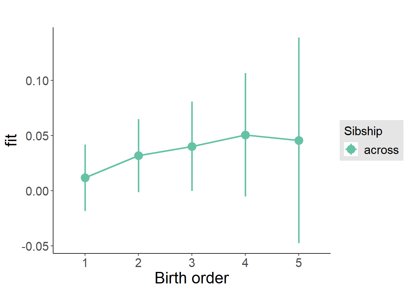
Add Interaction
Model Summary
m4_interaction = update(m3_birthorder_nonlinear, formula = . ~ . - birth_order_nonlinear - sibling_count + count_birth_order)
tidy(m4_interaction, conf.int = T, conf.level = 0.995)| effect | group | term | estimate | std.error | statistic | df | p.value | conf.low | conf.high |
|---|---|---|---|---|---|---|---|---|---|
| fixed | NA | (Intercept) | 2.747 | 0.2374 | 11.57 | 2735 | 2.82e-30 | 2.081 | 3.413 |
| fixed | NA | poly(age, 3, raw = TRUE)1 | -0.2576 | 0.02636 | -9.772 | 2735 | 3.411e-22 | -0.3316 | -0.1836 |
| fixed | NA | poly(age, 3, raw = TRUE)2 | 0.007893 | 0.000937 | 8.424 | 2735 | 5.782e-17 | 0.005263 | 0.01052 |
| fixed | NA | poly(age, 3, raw = TRUE)3 | -0.00007851 | 0.00001067 | -7.358 | 2733 | 2.459e-13 | -0.0001085 | -0.00004856 |
| fixed | NA | male | -0.01993 | 0.01101 | -1.81 | 2721 | 0.0704 | -0.05084 | 0.01098 |
| fixed | NA | count_birth_order2/2 | 0.01965 | 0.02329 | 0.8439 | 2146 | 0.3988 | -0.04571 | 0.08502 |
| fixed | NA | count_birth_order1/3 | 0.006341 | 0.0199 | 0.3187 | 2745 | 0.75 | -0.04952 | 0.0622 |
| fixed | NA | count_birth_order2/3 | 0.04274 | 0.02213 | 1.931 | 2749 | 0.05354 | -0.01938 | 0.1049 |
| fixed | NA | count_birth_order3/3 | 0.06814 | 0.0237 | 2.875 | 2741 | 0.004069 | 0.001615 | 0.1347 |
| fixed | NA | count_birth_order1/4 | 0.04763 | 0.0234 | 2.035 | 2750 | 0.04192 | -0.01806 | 0.1133 |
| fixed | NA | count_birth_order2/4 | 0.04463 | 0.02443 | 1.827 | 2746 | 0.06782 | -0.02394 | 0.1132 |
| fixed | NA | count_birth_order3/4 | 0.04469 | 0.0256 | 1.745 | 2736 | 0.08101 | -0.02718 | 0.1166 |
| fixed | NA | count_birth_order4/4 | 0.07156 | 0.02758 | 2.594 | 2734 | 0.009532 | -0.005871 | 0.149 |
| fixed | NA | count_birth_order1/5 | 0.05139 | 0.03069 | 1.675 | 2749 | 0.09413 | -0.03475 | 0.1375 |
| fixed | NA | count_birth_order2/5 | 0.06487 | 0.03438 | 1.887 | 2720 | 0.05932 | -0.03165 | 0.1614 |
| fixed | NA | count_birth_order3/5 | 0.04752 | 0.03288 | 1.445 | 2719 | 0.1485 | -0.04477 | 0.1398 |
| fixed | NA | count_birth_order4/5 | 0.07415 | 0.03168 | 2.341 | 2719 | 0.01932 | -0.01478 | 0.1631 |
| fixed | NA | count_birth_order5/5 | 0.07159 | 0.03334 | 2.147 | 2712 | 0.03186 | -0.022 | 0.1652 |
| ran_pars | mother_pidlink | sd__(Intercept) | 0.09081 | NA | NA | NA | NA | NA | NA |
| ran_pars | Residual | sd__Observation | 0.2709 | NA | NA | NA | NA | NA | NA |
Coefficient Plot
plot_birthorder(m4_interaction)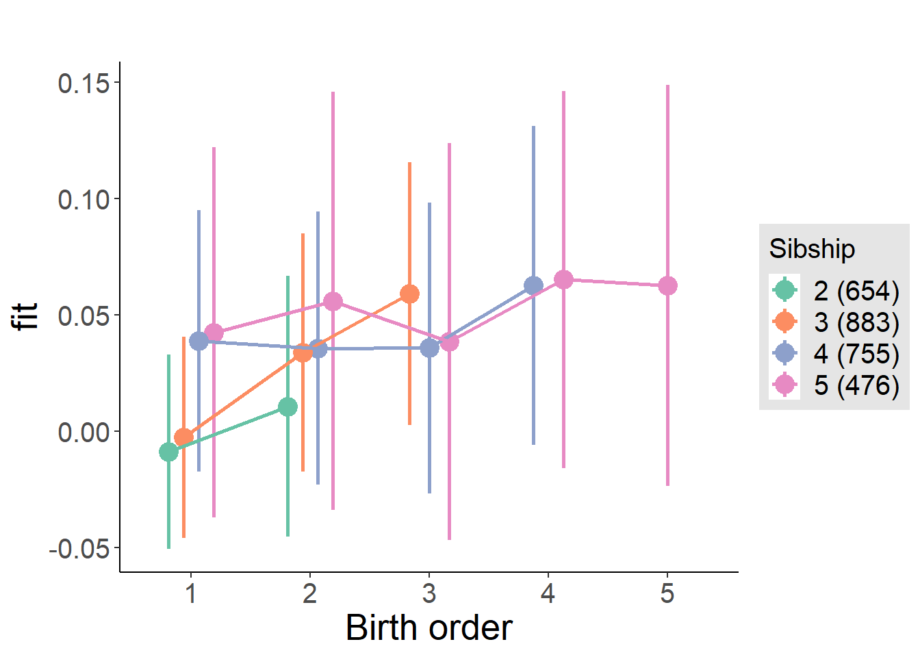
Model Comparison
###### Model 1 - Model 2
anova(m1_covariates_only, m2_birthorder_linear, m3_birthorder_nonlinear, m4_interaction)## refitting model(s) with ML (instead of REML)| Df | AIC | BIC | logLik | deviance | Chisq | Chi Df | Pr(>Chisq) |
|---|---|---|---|---|---|---|---|
| 10 | 921.7 | 980.9 | -450.8 | 901.7 | NA | NA | NA |
| 11 | 918.9 | 984.1 | -448.4 | 896.9 | 4.819 | 1 | 0.02815 |
| 14 | 924.2 | 1007 | -448.1 | 896.2 | 0.6643 | 3 | 0.8816 |
| 20 | 932 | 1051 | -446 | 892 | 4.182 | 6 | 0.6521 |
Compare birth order specifications
library(coefplot)
multiplot(outcome_naive_m1, outcome_preg_m1, outcome_uterus_m1, outcome_parental_m1, dodgeHeight = 0.6,
intercept = FALSE)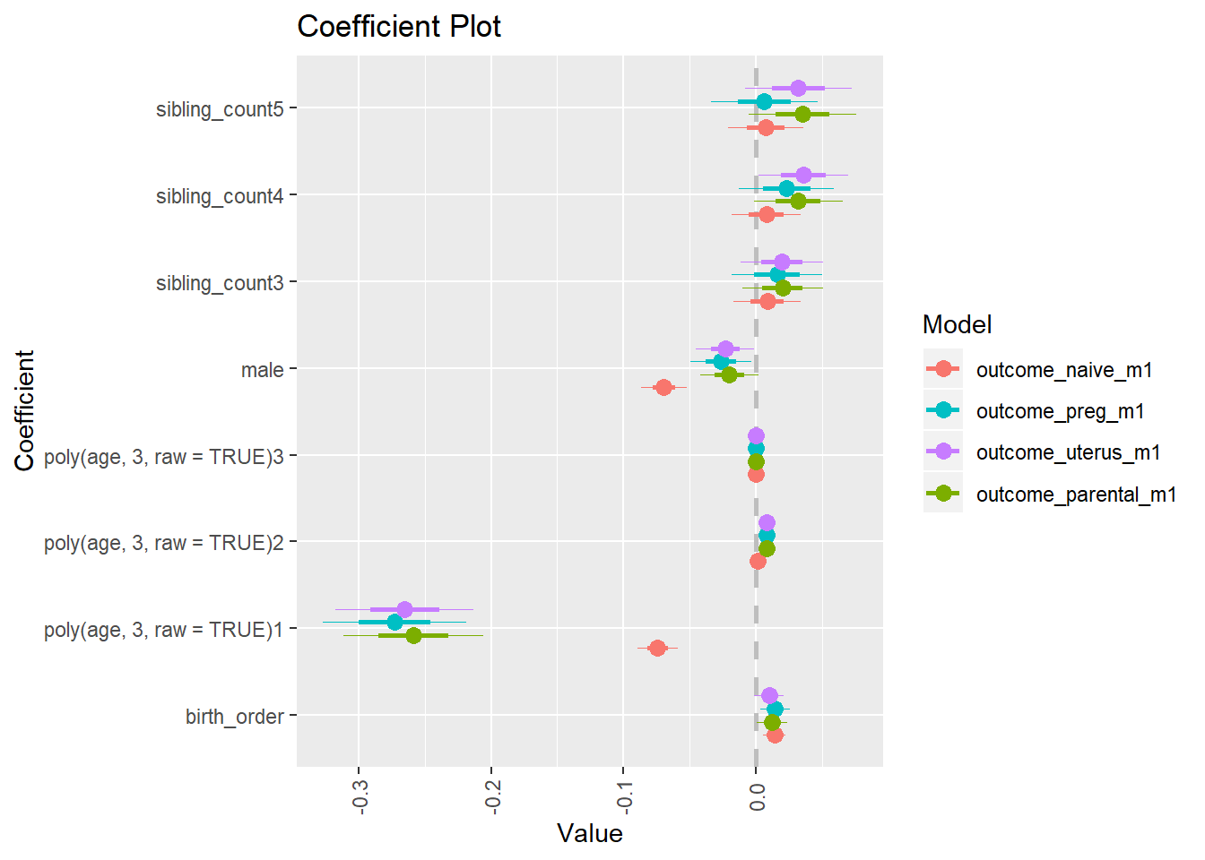
Work Sector
Sector_Agriculture, forestry, fishing and hunting
birthorder <- birthorder %>% mutate(outcome = `Sector_Agriculture, forestry, fishing and hunting`)
model = lmer(outcome ~ birth_order + poly(age, 3, raw = TRUE) + male + sibling_count + (1 | mother_pidlink),
data = birthorder)
compare_birthorder_specs(model)Naive birth order
outcome_naive_m1 <- update(m2_birthorder_linear, data = birthorder %>%
mutate(sibling_count = sibling_count_naive_factor,
birth_order_nonlinear = birthorder_naive_factor,
birth_order = birthorder_naive,
count_birth_order = count_birthorder_naive) %>%
filter(sibling_count != "1"))
compare_models_markdown(outcome_naive_m1)Basic Model
Model Summary
m1_covariates_only <- update(m2_birthorder_linear, formula = . ~ . - birth_order)
tidy(m1_covariates_only, conf.int = T, conf.level = 0.995)| effect | group | term | estimate | std.error | statistic | df | p.value | conf.low | conf.high |
|---|---|---|---|---|---|---|---|---|---|
| fixed | NA | (Intercept) | 0.1096 | 0.1173 | 0.935 | 4355 | 0.3498 | -0.2195 | 0.4388 |
| fixed | NA | poly(age, 3, raw = TRUE)1 | -0.0003363 | 0.01045 | -0.03218 | 4269 | 0.9743 | -0.02967 | 0.029 |
| fixed | NA | poly(age, 3, raw = TRUE)2 | 0.0001506 | 0.0002899 | 0.5197 | 4162 | 0.6033 | -0.0006631 | 0.0009643 |
| fixed | NA | poly(age, 3, raw = TRUE)3 | -0.000001799 | 0.000002532 | -0.7107 | 4062 | 0.4773 | -0.000008906 | 0.000005307 |
| fixed | NA | male | 0.02245 | 0.01177 | 1.907 | 4520 | 0.05659 | -0.01059 | 0.05549 |
| fixed | NA | sibling_count3 | 0.003521 | 0.01738 | 0.2025 | 3347 | 0.8395 | -0.04528 | 0.05232 |
| fixed | NA | sibling_count4 | 0.002892 | 0.01763 | 0.164 | 3164 | 0.8697 | -0.0466 | 0.05238 |
| fixed | NA | sibling_count5 | 0.002738 | 0.01839 | 0.1489 | 2976 | 0.8817 | -0.04888 | 0.05436 |
| ran_pars | mother_pidlink | sd__(Intercept) | 0.1729 | NA | NA | NA | NA | NA | NA |
| ran_pars | Residual | sd__Observation | 0.3632 | NA | NA | NA | NA | NA | NA |
Coefficient Plot
plot(allEffects(m1_covariates_only, confidence.level = 0.995))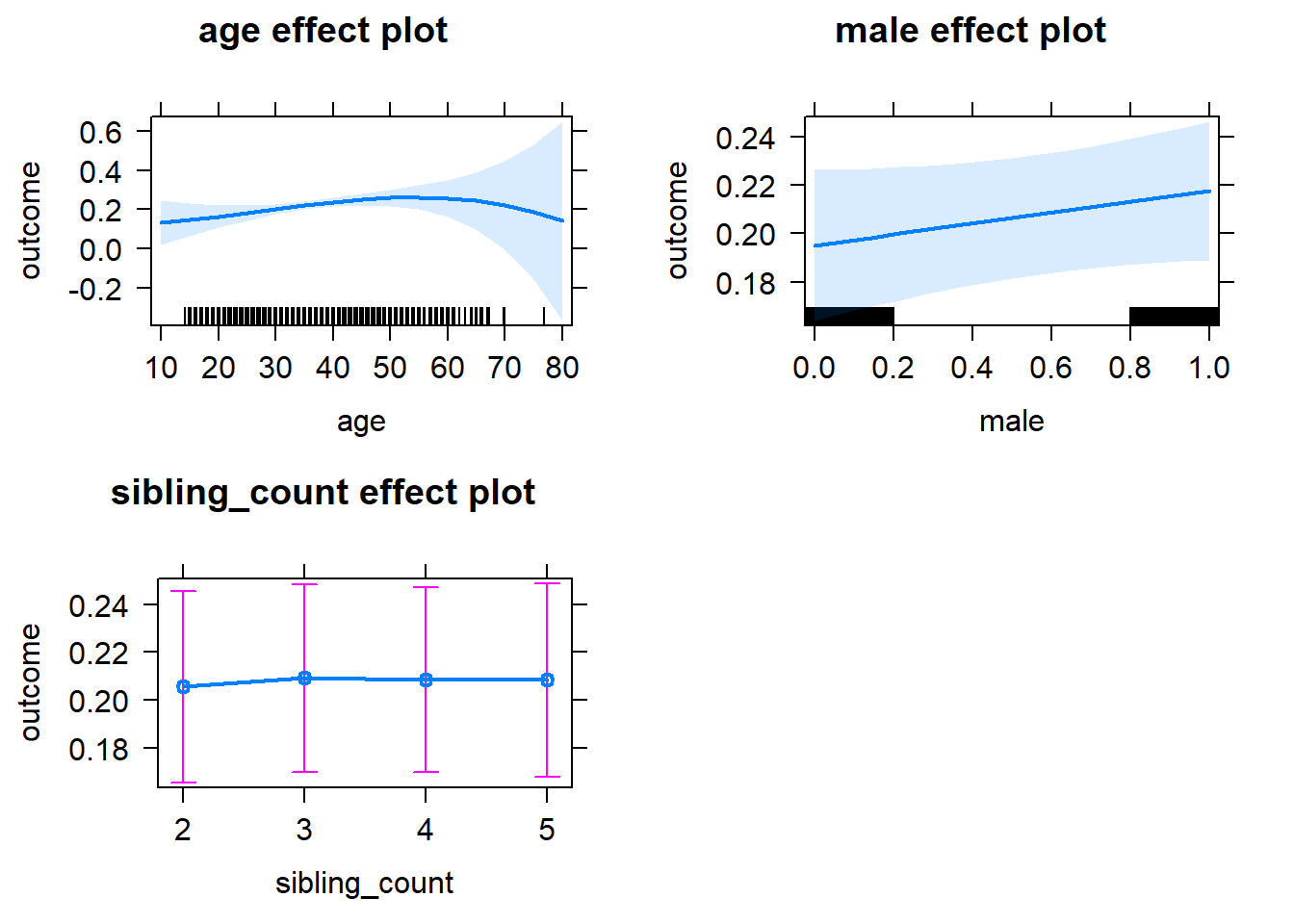
Add Birth Order Linear
Model Summary
tidy(m2_birthorder_linear, conf.int = T, conf.level = 0.995)| effect | group | term | estimate | std.error | statistic | df | p.value | conf.low | conf.high |
|---|---|---|---|---|---|---|---|---|---|
| fixed | NA | (Intercept) | 0.1123 | 0.1172 | 0.9582 | 4356 | 0.338 | -0.2168 | 0.4414 |
| fixed | NA | birth_order | 0.01095 | 0.005734 | 1.91 | 3967 | 0.05617 | -0.005142 | 0.02705 |
| fixed | NA | poly(age, 3, raw = TRUE)1 | -0.002077 | 0.01049 | -0.1981 | 4271 | 0.843 | -0.03151 | 0.02736 |
| fixed | NA | poly(age, 3, raw = TRUE)2 | 0.0001954 | 0.0002907 | 0.672 | 4155 | 0.5016 | -0.0006208 | 0.001012 |
| fixed | NA | poly(age, 3, raw = TRUE)3 | -0.000002106 | 0.000002536 | -0.8305 | 4055 | 0.4063 | -0.000009225 | 0.000005013 |
| fixed | NA | male | 0.02261 | 0.01177 | 1.921 | 4519 | 0.05476 | -0.01042 | 0.05564 |
| fixed | NA | sibling_count3 | -0.0004637 | 0.0175 | -0.02649 | 3426 | 0.9789 | -0.0496 | 0.04867 |
| fixed | NA | sibling_count4 | -0.005752 | 0.0182 | -0.3161 | 3484 | 0.7519 | -0.05683 | 0.04533 |
| fixed | NA | sibling_count5 | -0.01102 | 0.01975 | -0.5582 | 3613 | 0.5768 | -0.06645 | 0.04441 |
| ran_pars | mother_pidlink | sd__(Intercept) | 0.1729 | NA | NA | NA | NA | NA | NA |
| ran_pars | Residual | sd__Observation | 0.363 | NA | NA | NA | NA | NA | NA |
Coefficient Plot
plot_birthorder2(m2_birthorder_linear, separate = FALSE)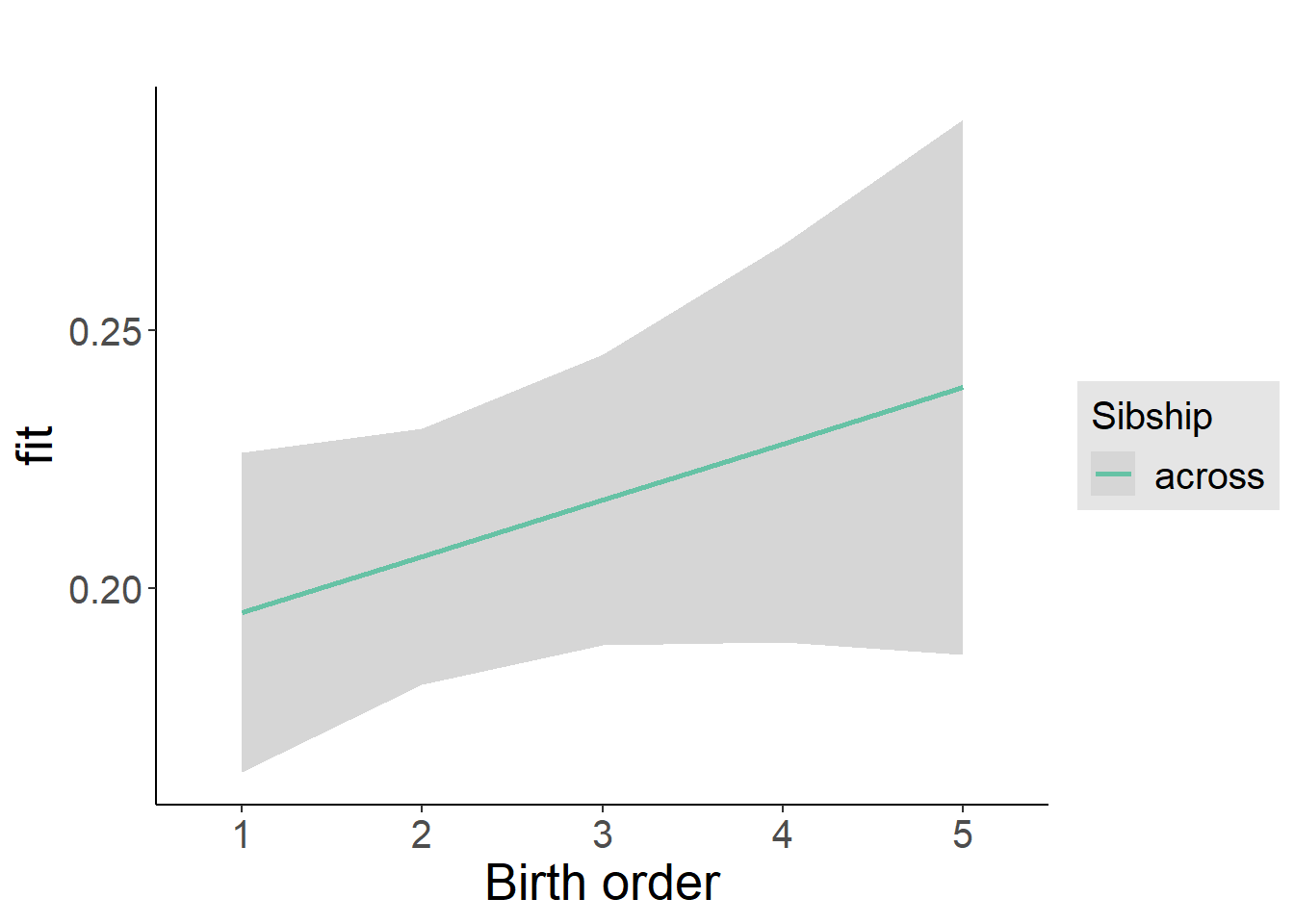
Add Birth Order Factor
Model Summary
m3_birthorder_nonlinear = update(m1_covariates_only, formula = . ~ . + birth_order_nonlinear)
tidy(m3_birthorder_nonlinear, conf.int = T, conf.level = 0.995)| effect | group | term | estimate | std.error | statistic | df | p.value | conf.low | conf.high |
|---|---|---|---|---|---|---|---|---|---|
| fixed | NA | (Intercept) | 0.139 | 0.1175 | 1.183 | 4360 | 0.2371 | -0.1909 | 0.4689 |
| fixed | NA | poly(age, 3, raw = TRUE)1 | -0.002807 | 0.01048 | -0.2678 | 4265 | 0.7889 | -0.03224 | 0.02662 |
| fixed | NA | poly(age, 3, raw = TRUE)2 | 0.0002178 | 0.0002908 | 0.7491 | 4145 | 0.4538 | -0.0005984 | 0.001034 |
| fixed | NA | poly(age, 3, raw = TRUE)3 | -0.000002315 | 0.000002538 | -0.9124 | 4038 | 0.3616 | -0.000009439 | 0.000004808 |
| fixed | NA | male | 0.02272 | 0.01176 | 1.932 | 4514 | 0.05344 | -0.01029 | 0.05574 |
| fixed | NA | sibling_count3 | -0.006273 | 0.01776 | -0.3531 | 3558 | 0.724 | -0.05614 | 0.04359 |
| fixed | NA | sibling_count4 | -0.01525 | 0.01848 | -0.8252 | 3628 | 0.4093 | -0.06713 | 0.03663 |
| fixed | NA | sibling_count5 | -0.01281 | 0.01991 | -0.6433 | 3694 | 0.5201 | -0.0687 | 0.04308 |
| fixed | NA | birth_order_nonlinear2 | -0.01236 | 0.0138 | -0.8957 | 3919 | 0.3704 | -0.0511 | 0.02638 |
| fixed | NA | birth_order_nonlinear3 | 0.04099 | 0.01747 | 2.346 | 3815 | 0.01904 | -0.00806 | 0.09004 |
| fixed | NA | birth_order_nonlinear4 | 0.04802 | 0.0228 | 2.106 | 3716 | 0.03528 | -0.01599 | 0.112 |
| fixed | NA | birth_order_nonlinear5 | -0.003216 | 0.03293 | -0.09765 | 3745 | 0.9222 | -0.09566 | 0.08923 |
| ran_pars | mother_pidlink | sd__(Intercept) | 0.1732 | NA | NA | NA | NA | NA | NA |
| ran_pars | Residual | sd__Observation | 0.3626 | NA | NA | NA | NA | NA | NA |
Coefficient Plot
plot_birthorder(m3_birthorder_nonlinear, separate = FALSE)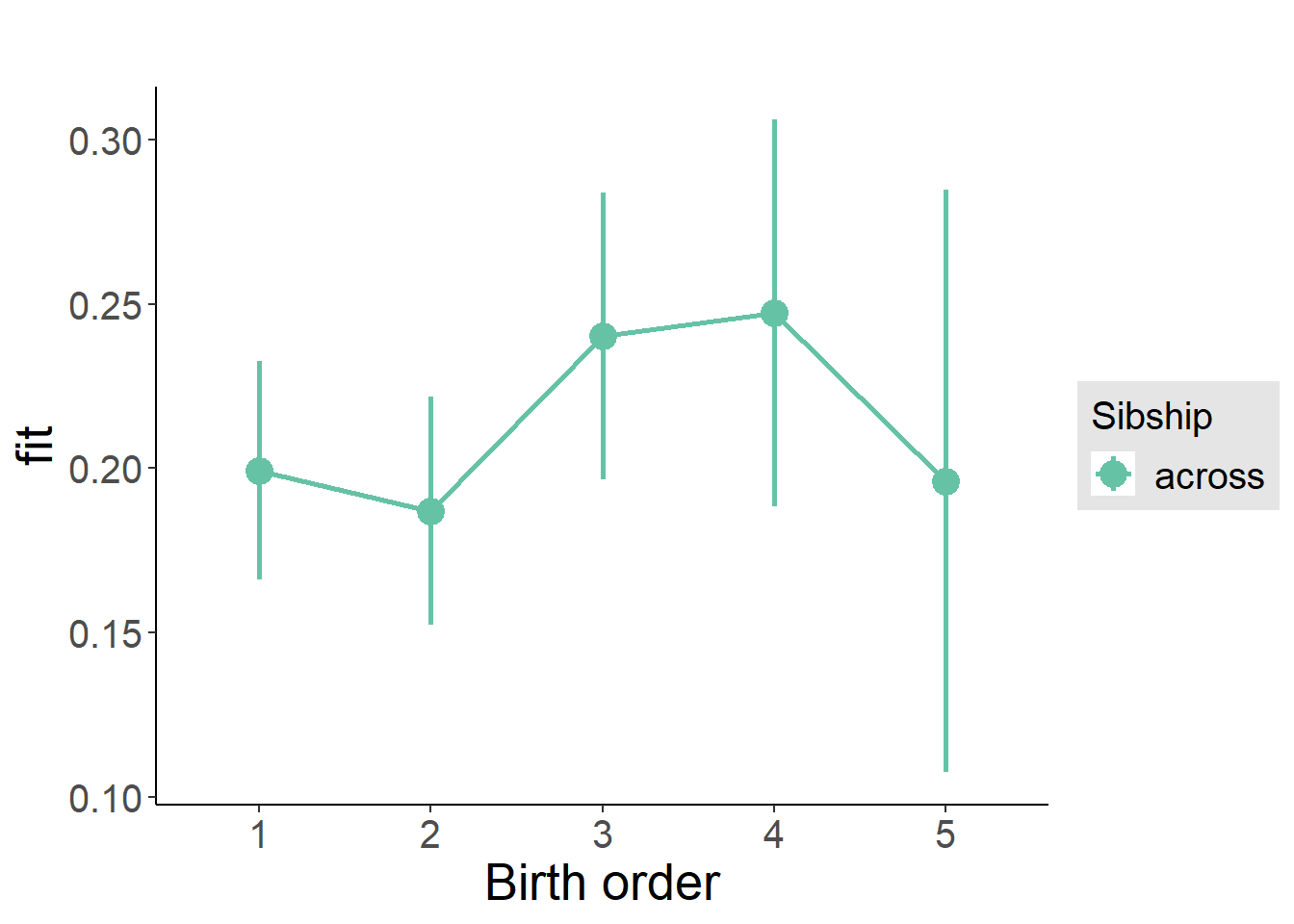
Add Interaction
Model Summary
m4_interaction = update(m3_birthorder_nonlinear, formula = . ~ . - birth_order_nonlinear - sibling_count + count_birth_order)
tidy(m4_interaction, conf.int = T, conf.level = 0.995)| effect | group | term | estimate | std.error | statistic | df | p.value | conf.low | conf.high |
|---|---|---|---|---|---|---|---|---|---|
| fixed | NA | (Intercept) | 0.1517 | 0.1176 | 1.29 | 4365 | 0.1972 | -0.1785 | 0.482 |
| fixed | NA | poly(age, 3, raw = TRUE)1 | -0.003214 | 0.01049 | -0.3064 | 4266 | 0.7593 | -0.03266 | 0.02623 |
| fixed | NA | poly(age, 3, raw = TRUE)2 | 0.0002279 | 0.0002908 | 0.7837 | 4146 | 0.4333 | -0.0005884 | 0.001044 |
| fixed | NA | poly(age, 3, raw = TRUE)3 | -0.00000239 | 0.000002537 | -0.9417 | 4039 | 0.3464 | -0.000009512 | 0.000004733 |
| fixed | NA | male | 0.02228 | 0.01176 | 1.895 | 4505 | 0.05818 | -0.01073 | 0.05529 |
| fixed | NA | count_birth_order2/2 | -0.03319 | 0.02345 | -1.415 | 3905 | 0.1571 | -0.09901 | 0.03264 |
| fixed | NA | count_birth_order1/3 | -0.02716 | 0.02295 | -1.184 | 4604 | 0.2366 | -0.09158 | 0.03725 |
| fixed | NA | count_birth_order2/3 | -0.02609 | 0.0255 | -1.023 | 4623 | 0.3063 | -0.09769 | 0.0455 |
| fixed | NA | count_birth_order3/3 | 0.05206 | 0.02802 | 1.858 | 4624 | 0.06327 | -0.0266 | 0.1307 |
| fixed | NA | count_birth_order1/4 | -0.02378 | 0.02524 | -0.9422 | 4623 | 0.3461 | -0.09462 | 0.04706 |
| fixed | NA | count_birth_order2/4 | -0.03995 | 0.02706 | -1.476 | 4625 | 0.1399 | -0.1159 | 0.03601 |
| fixed | NA | count_birth_order3/4 | 0.03713 | 0.02853 | 1.301 | 4622 | 0.1932 | -0.04296 | 0.1172 |
| fixed | NA | count_birth_order4/4 | 0.009843 | 0.03074 | 0.3202 | 4612 | 0.7488 | -0.07645 | 0.09614 |
| fixed | NA | count_birth_order1/5 | -0.01435 | 0.02841 | -0.505 | 4622 | 0.6136 | -0.09411 | 0.06541 |
| fixed | NA | count_birth_order2/5 | -0.001036 | 0.03018 | -0.03433 | 4616 | 0.9726 | -0.08574 | 0.08367 |
| fixed | NA | count_birth_order3/5 | -0.04063 | 0.03172 | -1.281 | 4601 | 0.2003 | -0.1297 | 0.04841 |
| fixed | NA | count_birth_order4/5 | 0.0471 | 0.03346 | 1.408 | 4561 | 0.1593 | -0.04682 | 0.141 |
| fixed | NA | count_birth_order5/5 | -0.02448 | 0.03359 | -0.7289 | 4589 | 0.4661 | -0.1188 | 0.0698 |
| ran_pars | mother_pidlink | sd__(Intercept) | 0.1736 | NA | NA | NA | NA | NA | NA |
| ran_pars | Residual | sd__Observation | 0.3622 | NA | NA | NA | NA | NA | NA |
Coefficient Plot
plot_birthorder(m4_interaction)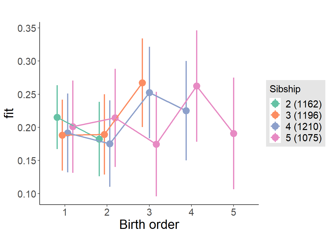
Model Comparison
###### Model 1 - Model 2
anova(m1_covariates_only, m2_birthorder_linear, m3_birthorder_nonlinear, m4_interaction)## refitting model(s) with ML (instead of REML)| Df | AIC | BIC | logLik | deviance | Chisq | Chi Df | Pr(>Chisq) |
|---|---|---|---|---|---|---|---|
| 10 | 4670 | 4734 | -2325 | 4650 | NA | NA | NA |
| 11 | 4668 | 4739 | -2323 | 4646 | 3.654 | 1 | 0.05595 |
| 14 | 4665 | 4755 | -2318 | 4637 | 9.263 | 3 | 0.02599 |
| 20 | 4666 | 4795 | -2313 | 4626 | 11 | 6 | 0.08848 |
Maternal birth order
outcome_uterus_m1 <- update(m2_birthorder_linear, data = birthorder %>%
mutate(sibling_count = sibling_count_uterus_alive_factor,
birth_order_nonlinear = birthorder_uterus_alive_factor,
birth_order = birthorder_uterus_alive,
count_birth_order = count_birthorder_uterus_alive) %>%
filter(sibling_count != "1"))
compare_models_markdown(outcome_uterus_m1)Basic Model
Model Summary
m1_covariates_only <- update(m2_birthorder_linear, formula = . ~ . - birth_order)
tidy(m1_covariates_only, conf.int = T, conf.level = 0.995)| effect | group | term | estimate | std.error | statistic | df | p.value | conf.low | conf.high |
|---|---|---|---|---|---|---|---|---|---|
| fixed | NA | (Intercept) | 0.4298 | 0.3118 | 1.378 | 2632 | 0.1682 | -0.4455 | 1.305 |
| fixed | NA | poly(age, 3, raw = TRUE)1 | -0.03507 | 0.03451 | -1.016 | 2633 | 0.3096 | -0.1319 | 0.0618 |
| fixed | NA | poly(age, 3, raw = TRUE)2 | 0.001356 | 0.001222 | 1.109 | 2633 | 0.2675 | -0.002076 | 0.004787 |
| fixed | NA | poly(age, 3, raw = TRUE)3 | -0.00001569 | 0.00001387 | -1.131 | 2633 | 0.258 | -0.00005462 | 0.00002324 |
| fixed | NA | male | 0.01584 | 0.01462 | 1.084 | 2608 | 0.2786 | -0.02519 | 0.05687 |
| fixed | NA | sibling_count3 | -0.01764 | 0.02064 | -0.8545 | 2071 | 0.393 | -0.07557 | 0.0403 |
| fixed | NA | sibling_count4 | -0.006795 | 0.02141 | -0.3173 | 1912 | 0.751 | -0.0669 | 0.05331 |
| fixed | NA | sibling_count5 | 0.005005 | 0.02395 | 0.209 | 1682 | 0.8345 | -0.06223 | 0.07225 |
| ran_pars | mother_pidlink | sd__(Intercept) | 0.1401 | NA | NA | NA | NA | NA | NA |
| ran_pars | Residual | sd__Observation | 0.3446 | NA | NA | NA | NA | NA | NA |
Coefficient Plot
plot(allEffects(m1_covariates_only, confidence.level = 0.995))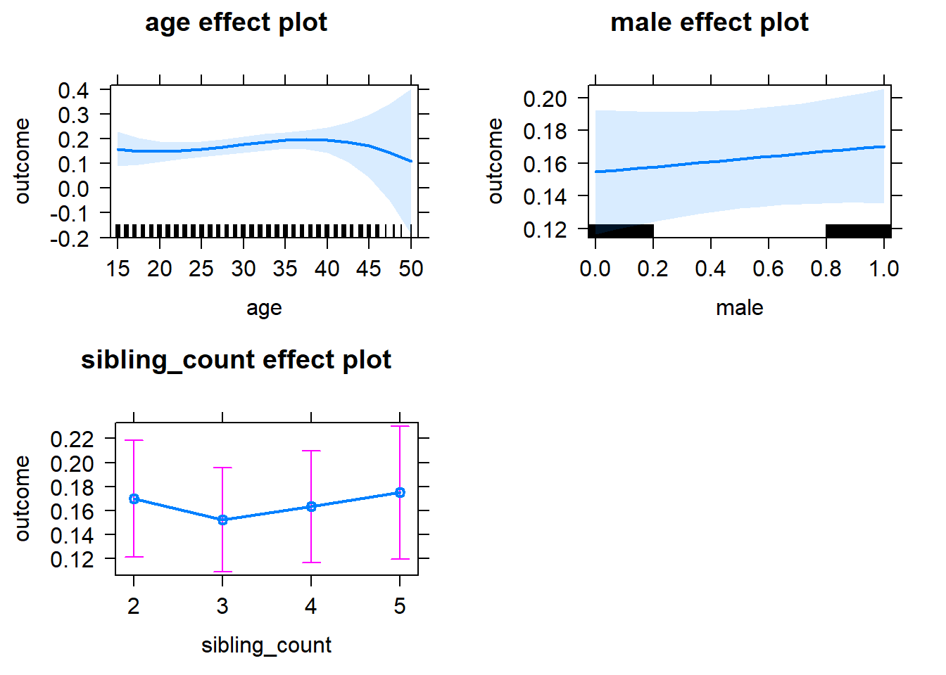
Add Birth Order Linear
Model Summary
tidy(m2_birthorder_linear, conf.int = T, conf.level = 0.995)| effect | group | term | estimate | std.error | statistic | df | p.value | conf.low | conf.high |
|---|---|---|---|---|---|---|---|---|---|
| fixed | NA | (Intercept) | 0.4294 | 0.3119 | 1.377 | 2631 | 0.1686 | -0.446 | 1.305 |
| fixed | NA | birth_order | 0.005404 | 0.007337 | 0.7365 | 2443 | 0.4615 | -0.01519 | 0.026 |
| fixed | NA | poly(age, 3, raw = TRUE)1 | -0.03567 | 0.03452 | -1.033 | 2631 | 0.3015 | -0.1326 | 0.06123 |
| fixed | NA | poly(age, 3, raw = TRUE)2 | 0.001368 | 0.001223 | 1.119 | 2632 | 0.2633 | -0.002064 | 0.0048 |
| fixed | NA | poly(age, 3, raw = TRUE)3 | -0.00001568 | 0.00001387 | -1.131 | 2632 | 0.2584 | -0.00005461 | 0.00002325 |
| fixed | NA | male | 0.01584 | 0.01462 | 1.084 | 2607 | 0.2785 | -0.02519 | 0.05688 |
| fixed | NA | sibling_count3 | -0.02019 | 0.02093 | -0.9647 | 2103 | 0.3348 | -0.07895 | 0.03856 |
| fixed | NA | sibling_count4 | -0.01235 | 0.02271 | -0.544 | 2036 | 0.5865 | -0.07609 | 0.05138 |
| fixed | NA | sibling_count5 | -0.004252 | 0.02705 | -0.1572 | 1997 | 0.8751 | -0.08019 | 0.07169 |
| ran_pars | mother_pidlink | sd__(Intercept) | 0.1402 | NA | NA | NA | NA | NA | NA |
| ran_pars | Residual | sd__Observation | 0.3446 | NA | NA | NA | NA | NA | NA |
Coefficient Plot
plot_birthorder2(m2_birthorder_linear, separate = FALSE)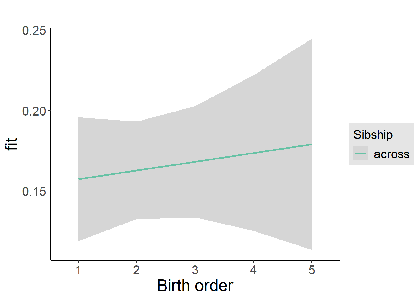
Add Birth Order Factor
Model Summary
m3_birthorder_nonlinear = update(m1_covariates_only, formula = . ~ . + birth_order_nonlinear)
tidy(m3_birthorder_nonlinear, conf.int = T, conf.level = 0.995)| effect | group | term | estimate | std.error | statistic | df | p.value | conf.low | conf.high |
|---|---|---|---|---|---|---|---|---|---|
| fixed | NA | (Intercept) | 0.3941 | 0.3123 | 1.262 | 2628 | 0.2071 | -0.4825 | 1.271 |
| fixed | NA | poly(age, 3, raw = TRUE)1 | -0.03118 | 0.03455 | -0.9025 | 2628 | 0.3669 | -0.1282 | 0.0658 |
| fixed | NA | poly(age, 3, raw = TRUE)2 | 0.001212 | 0.001224 | 0.9908 | 2628 | 0.3219 | -0.002222 | 0.004647 |
| fixed | NA | poly(age, 3, raw = TRUE)3 | -0.00001401 | 0.00001388 | -1.01 | 2628 | 0.3127 | -0.00005297 | 0.00002494 |
| fixed | NA | male | 0.01663 | 0.01462 | 1.137 | 2606 | 0.2555 | -0.02441 | 0.05767 |
| fixed | NA | sibling_count3 | -0.02898 | 0.02121 | -1.366 | 2161 | 0.172 | -0.08851 | 0.03055 |
| fixed | NA | sibling_count4 | -0.0191 | 0.02297 | -0.8312 | 2090 | 0.406 | -0.08358 | 0.04539 |
| fixed | NA | sibling_count5 | 0.00167 | 0.02735 | 0.06106 | 2041 | 0.9513 | -0.0751 | 0.07844 |
| fixed | NA | birth_order_nonlinear2 | 0.006427 | 0.01745 | 0.3683 | 2221 | 0.7127 | -0.04256 | 0.05541 |
| fixed | NA | birth_order_nonlinear3 | 0.04921 | 0.02129 | 2.312 | 2257 | 0.02088 | -0.01055 | 0.109 |
| fixed | NA | birth_order_nonlinear4 | 0.007926 | 0.02838 | 0.2793 | 2318 | 0.78 | -0.07173 | 0.08759 |
| fixed | NA | birth_order_nonlinear5 | -0.03822 | 0.04392 | -0.8702 | 2233 | 0.3843 | -0.1615 | 0.08506 |
| ran_pars | mother_pidlink | sd__(Intercept) | 0.1398 | NA | NA | NA | NA | NA | NA |
| ran_pars | Residual | sd__Observation | 0.3445 | NA | NA | NA | NA | NA | NA |
Coefficient Plot
plot_birthorder(m3_birthorder_nonlinear, separate = FALSE)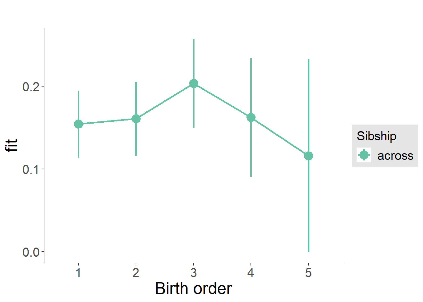
Add Interaction
Model Summary
m4_interaction = update(m3_birthorder_nonlinear, formula = . ~ . - birth_order_nonlinear - sibling_count + count_birth_order)
tidy(m4_interaction, conf.int = T, conf.level = 0.995)| effect | group | term | estimate | std.error | statistic | df | p.value | conf.low | conf.high |
|---|---|---|---|---|---|---|---|---|---|
| fixed | NA | (Intercept) | 0.3924 | 0.3125 | 1.256 | 2621 | 0.2094 | -0.4848 | 1.27 |
| fixed | NA | poly(age, 3, raw = TRUE)1 | -0.03153 | 0.03458 | -0.9119 | 2622 | 0.3619 | -0.1286 | 0.06553 |
| fixed | NA | poly(age, 3, raw = TRUE)2 | 0.001212 | 0.001225 | 0.9899 | 2622 | 0.3223 | -0.002225 | 0.00465 |
| fixed | NA | poly(age, 3, raw = TRUE)3 | -0.00001388 | 0.00001389 | -0.999 | 2622 | 0.3179 | -0.00005288 | 0.00002512 |
| fixed | NA | male | 0.016 | 0.01464 | 1.092 | 2601 | 0.2747 | -0.02511 | 0.0571 |
| fixed | NA | count_birth_order2/2 | 0.03144 | 0.03185 | 0.9872 | 2253 | 0.3237 | -0.05796 | 0.1208 |
| fixed | NA | count_birth_order1/3 | -0.006786 | 0.0269 | -0.2523 | 2620 | 0.8008 | -0.08229 | 0.06871 |
| fixed | NA | count_birth_order2/3 | -0.03196 | 0.02987 | -1.07 | 2624 | 0.2848 | -0.1158 | 0.05189 |
| fixed | NA | count_birth_order3/3 | 0.02356 | 0.03252 | 0.7245 | 2619 | 0.4689 | -0.06772 | 0.1148 |
| fixed | NA | count_birth_order1/4 | -0.01457 | 0.03093 | -0.471 | 2624 | 0.6377 | -0.1014 | 0.07226 |
| fixed | NA | count_birth_order2/4 | 0.009346 | 0.03271 | 0.2857 | 2621 | 0.7751 | -0.08248 | 0.1012 |
| fixed | NA | count_birth_order3/4 | 0.0513 | 0.0339 | 1.513 | 2614 | 0.1303 | -0.04385 | 0.1465 |
| fixed | NA | count_birth_order4/4 | -0.0323 | 0.03624 | -0.8914 | 2611 | 0.3728 | -0.134 | 0.06942 |
| fixed | NA | count_birth_order1/5 | -0.001454 | 0.04081 | -0.03564 | 2622 | 0.9716 | -0.116 | 0.1131 |
| fixed | NA | count_birth_order2/5 | -0.001126 | 0.04385 | -0.02567 | 2602 | 0.9795 | -0.1242 | 0.122 |
| fixed | NA | count_birth_order3/5 | 0.04489 | 0.04164 | 1.078 | 2601 | 0.2811 | -0.07198 | 0.1618 |
| fixed | NA | count_birth_order4/5 | 0.05709 | 0.04057 | 1.407 | 2596 | 0.1595 | -0.0568 | 0.171 |
| fixed | NA | count_birth_order5/5 | -0.02803 | 0.04266 | -0.657 | 2588 | 0.5113 | -0.1478 | 0.09173 |
| ran_pars | mother_pidlink | sd__(Intercept) | 0.1373 | NA | NA | NA | NA | NA | NA |
| ran_pars | Residual | sd__Observation | 0.3455 | NA | NA | NA | NA | NA | NA |
Coefficient Plot
plot_birthorder(m4_interaction)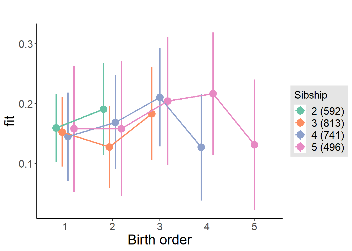
Model Comparison
###### Model 1 - Model 2
anova(m1_covariates_only, m2_birthorder_linear, m3_birthorder_nonlinear, m4_interaction)## refitting model(s) with ML (instead of REML)| Df | AIC | BIC | logLik | deviance | Chisq | Chi Df | Pr(>Chisq) |
|---|---|---|---|---|---|---|---|
| 10 | 2268 | 2327 | -1124 | 2248 | NA | NA | NA |
| 11 | 2270 | 2335 | -1124 | 2248 | 0.5435 | 1 | 0.461 |
| 14 | 2269 | 2351 | -1120 | 2241 | 6.918 | 3 | 0.07455 |
| 20 | 2276 | 2394 | -1118 | 2236 | 4.967 | 6 | 0.548 |
Maternal pregnancy order
outcome_preg_m1 <- update(m2_birthorder_linear, data = birthorder %>%
mutate(sibling_count = sibling_count_uterus_preg_factor,
birth_order_nonlinear = birthorder_uterus_preg_factor,
birth_order = birthorder_uterus_preg,
count_birth_order = count_birthorder_uterus_preg
) %>%
filter(sibling_count != "1"))
compare_models_markdown(outcome_preg_m1)Basic Model
Model Summary
m1_covariates_only <- update(m2_birthorder_linear, formula = . ~ . - birth_order)
tidy(m1_covariates_only, conf.int = T, conf.level = 0.995)| effect | group | term | estimate | std.error | statistic | df | p.value | conf.low | conf.high |
|---|---|---|---|---|---|---|---|---|---|
| fixed | NA | (Intercept) | 0.5068 | 0.3227 | 1.57 | 2418 | 0.1165 | -0.3991 | 1.413 |
| fixed | NA | poly(age, 3, raw = TRUE)1 | -0.04323 | 0.03574 | -1.21 | 2419 | 0.2266 | -0.1435 | 0.05709 |
| fixed | NA | poly(age, 3, raw = TRUE)2 | 0.001633 | 0.001266 | 1.29 | 2419 | 0.1971 | -0.00192 | 0.005187 |
| fixed | NA | poly(age, 3, raw = TRUE)3 | -0.00001865 | 0.00001436 | -1.299 | 2418 | 0.1942 | -0.00005898 | 0.00002167 |
| fixed | NA | male | 0.013 | 0.01525 | 0.8523 | 2395 | 0.3941 | -0.0298 | 0.0558 |
| fixed | NA | sibling_count3 | -0.02287 | 0.02262 | -1.011 | 1936 | 0.3122 | -0.08636 | 0.04063 |
| fixed | NA | sibling_count4 | -0.004911 | 0.02293 | -0.2142 | 1840 | 0.8304 | -0.06927 | 0.05945 |
| fixed | NA | sibling_count5 | 0.003723 | 0.02423 | 0.1537 | 1705 | 0.8779 | -0.06429 | 0.07174 |
| ran_pars | mother_pidlink | sd__(Intercept) | 0.1411 | NA | NA | NA | NA | NA | NA |
| ran_pars | Residual | sd__Observation | 0.344 | NA | NA | NA | NA | NA | NA |
Coefficient Plot
plot(allEffects(m1_covariates_only, confidence.level = 0.995))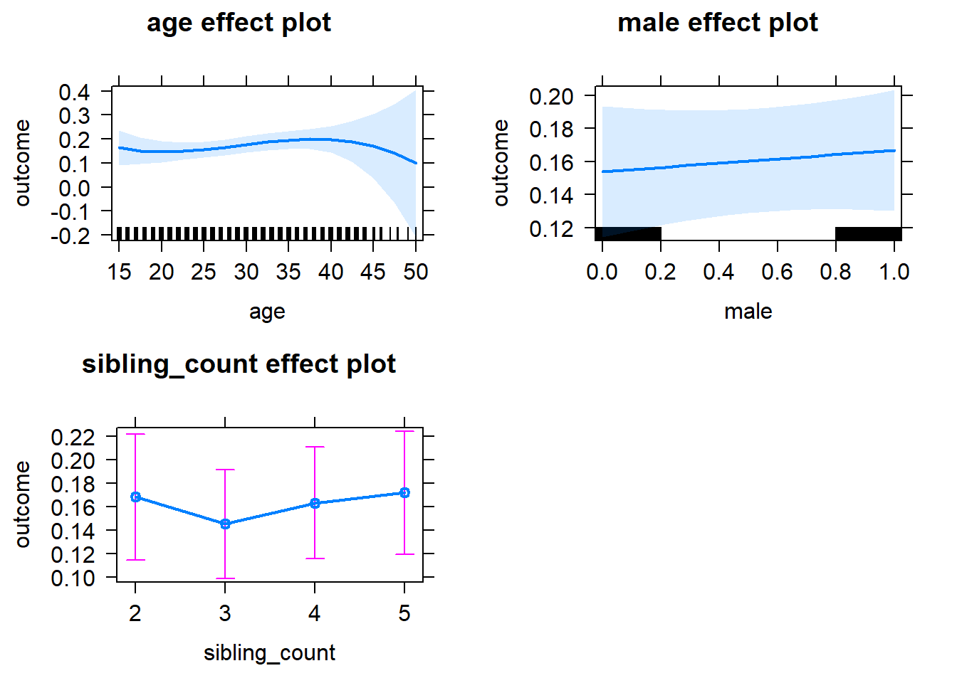
Add Birth Order Linear
Model Summary
tidy(m2_birthorder_linear, conf.int = T, conf.level = 0.995)| effect | group | term | estimate | std.error | statistic | df | p.value | conf.low | conf.high |
|---|---|---|---|---|---|---|---|---|---|
| fixed | NA | (Intercept) | 0.5047 | 0.3228 | 1.563 | 2418 | 0.1181 | -0.4014 | 1.411 |
| fixed | NA | birth_order | 0.00375 | 0.007449 | 0.5034 | 2300 | 0.6147 | -0.01716 | 0.02466 |
| fixed | NA | poly(age, 3, raw = TRUE)1 | -0.04349 | 0.03575 | -1.217 | 2418 | 0.2238 | -0.1438 | 0.05684 |
| fixed | NA | poly(age, 3, raw = TRUE)2 | 0.001638 | 0.001266 | 1.294 | 2418 | 0.1958 | -0.001916 | 0.005193 |
| fixed | NA | poly(age, 3, raw = TRUE)3 | -0.00001862 | 0.00001437 | -1.296 | 2418 | 0.1951 | -0.00005895 | 0.00002171 |
| fixed | NA | male | 0.01309 | 0.01525 | 0.8583 | 2394 | 0.3908 | -0.02972 | 0.0559 |
| fixed | NA | sibling_count3 | -0.02466 | 0.0229 | -1.077 | 1955 | 0.2817 | -0.08895 | 0.03963 |
| fixed | NA | sibling_count4 | -0.008467 | 0.024 | -0.3529 | 1913 | 0.7242 | -0.07583 | 0.05889 |
| fixed | NA | sibling_count5 | -0.002287 | 0.02701 | -0.08467 | 1924 | 0.9325 | -0.07812 | 0.07354 |
| ran_pars | mother_pidlink | sd__(Intercept) | 0.1412 | NA | NA | NA | NA | NA | NA |
| ran_pars | Residual | sd__Observation | 0.344 | NA | NA | NA | NA | NA | NA |
Coefficient Plot
plot_birthorder2(m2_birthorder_linear, separate = FALSE)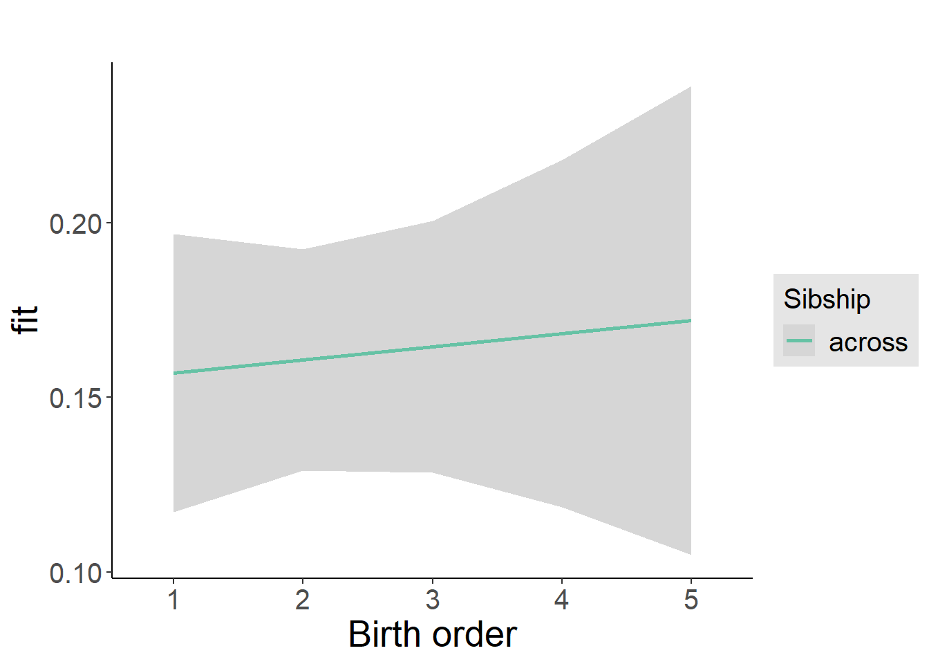
Add Birth Order Factor
Model Summary
m3_birthorder_nonlinear = update(m1_covariates_only, formula = . ~ . + birth_order_nonlinear)
tidy(m3_birthorder_nonlinear, conf.int = T, conf.level = 0.995)| effect | group | term | estimate | std.error | statistic | df | p.value | conf.low | conf.high |
|---|---|---|---|---|---|---|---|---|---|
| fixed | NA | (Intercept) | 0.4538 | 0.3234 | 1.403 | 2414 | 0.1607 | -0.4541 | 1.362 |
| fixed | NA | poly(age, 3, raw = TRUE)1 | -0.03751 | 0.0358 | -1.048 | 2414 | 0.2949 | -0.138 | 0.06299 |
| fixed | NA | poly(age, 3, raw = TRUE)2 | 0.001431 | 0.001268 | 1.128 | 2414 | 0.2594 | -0.002129 | 0.00499 |
| fixed | NA | poly(age, 3, raw = TRUE)3 | -0.00001637 | 0.00001439 | -1.138 | 2414 | 0.2552 | -0.00005676 | 0.00002401 |
| fixed | NA | male | 0.01364 | 0.01525 | 0.8947 | 2391 | 0.371 | -0.02916 | 0.05645 |
| fixed | NA | sibling_count3 | -0.03351 | 0.02319 | -1.445 | 2001 | 0.1485 | -0.0986 | 0.03157 |
| fixed | NA | sibling_count4 | -0.0166 | 0.02425 | -0.6845 | 1955 | 0.4937 | -0.08468 | 0.05148 |
| fixed | NA | sibling_count5 | 0.001543 | 0.02715 | 0.05683 | 1946 | 0.9547 | -0.07466 | 0.07775 |
| fixed | NA | birth_order_nonlinear2 | 0.005632 | 0.01808 | 0.3114 | 2047 | 0.7555 | -0.04513 | 0.05639 |
| fixed | NA | birth_order_nonlinear3 | 0.04672 | 0.02231 | 2.094 | 2124 | 0.03638 | -0.01591 | 0.1093 |
| fixed | NA | birth_order_nonlinear4 | 0.01262 | 0.02948 | 0.4281 | 2183 | 0.6687 | -0.07013 | 0.09537 |
| fixed | NA | birth_order_nonlinear5 | -0.04778 | 0.04225 | -1.131 | 2088 | 0.2583 | -0.1664 | 0.07083 |
| ran_pars | mother_pidlink | sd__(Intercept) | 0.141 | NA | NA | NA | NA | NA | NA |
| ran_pars | Residual | sd__Observation | 0.3438 | NA | NA | NA | NA | NA | NA |
Coefficient Plot
plot_birthorder(m3_birthorder_nonlinear, separate = FALSE)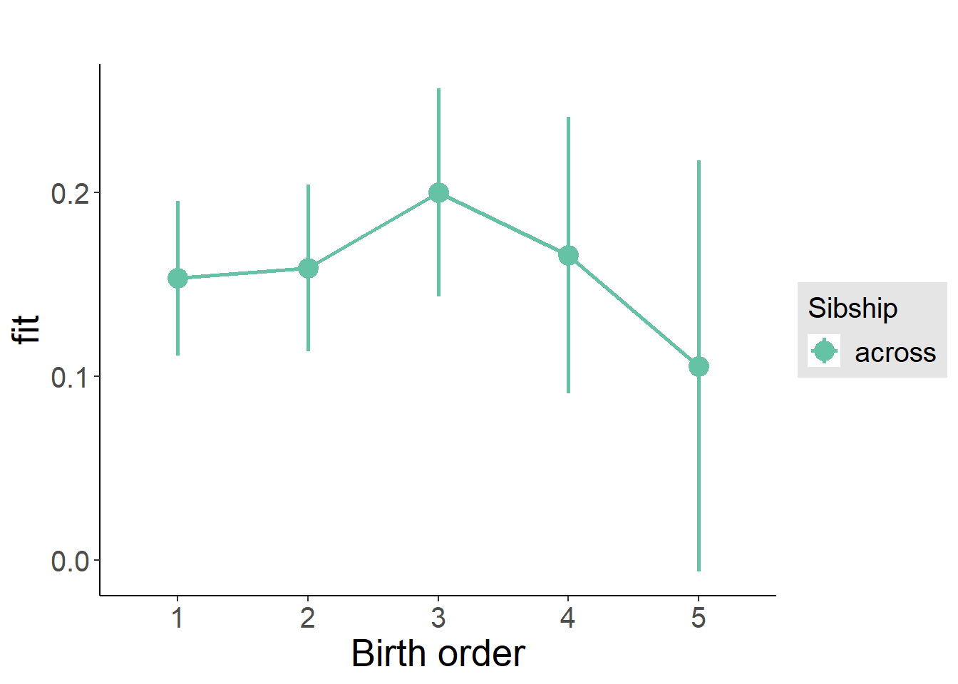
Add Interaction
Model Summary
m4_interaction = update(m3_birthorder_nonlinear, formula = . ~ . - birth_order_nonlinear - sibling_count + count_birth_order)
tidy(m4_interaction, conf.int = T, conf.level = 0.995)| effect | group | term | estimate | std.error | statistic | df | p.value | conf.low | conf.high |
|---|---|---|---|---|---|---|---|---|---|
| fixed | NA | (Intercept) | 0.4586 | 0.3237 | 1.417 | 2408 | 0.1567 | -0.4502 | 1.367 |
| fixed | NA | poly(age, 3, raw = TRUE)1 | -0.03856 | 0.03584 | -1.076 | 2408 | 0.2821 | -0.1392 | 0.06205 |
| fixed | NA | poly(age, 3, raw = TRUE)2 | 0.001456 | 0.00127 | 1.147 | 2408 | 0.2515 | -0.002108 | 0.00502 |
| fixed | NA | poly(age, 3, raw = TRUE)3 | -0.00001655 | 0.0000144 | -1.149 | 2408 | 0.2506 | -0.00005698 | 0.00002388 |
| fixed | NA | male | 0.01382 | 0.01528 | 0.904 | 2387 | 0.3661 | -0.02909 | 0.05672 |
| fixed | NA | count_birth_order2/2 | 0.02845 | 0.03493 | 0.8146 | 2128 | 0.4154 | -0.06959 | 0.1265 |
| fixed | NA | count_birth_order1/3 | -0.01219 | 0.02974 | -0.4098 | 2406 | 0.682 | -0.09567 | 0.0713 |
| fixed | NA | count_birth_order2/3 | -0.02868 | 0.03234 | -0.887 | 2409 | 0.3751 | -0.1195 | 0.06209 |
| fixed | NA | count_birth_order3/3 | 0.00595 | 0.03581 | 0.1661 | 2404 | 0.8681 | -0.09458 | 0.1065 |
| fixed | NA | count_birth_order1/4 | -0.02077 | 0.03237 | -0.6417 | 2408 | 0.5211 | -0.1116 | 0.07008 |
| fixed | NA | count_birth_order2/4 | -0.01071 | 0.03402 | -0.3148 | 2408 | 0.753 | -0.1062 | 0.0848 |
| fixed | NA | count_birth_order3/4 | 0.08524 | 0.03678 | 2.317 | 2400 | 0.02056 | -0.01801 | 0.1885 |
| fixed | NA | count_birth_order4/4 | -0.0201 | 0.03989 | -0.5039 | 2393 | 0.6144 | -0.1321 | 0.09186 |
| fixed | NA | count_birth_order1/5 | 0.0172 | 0.03916 | 0.4393 | 2408 | 0.6605 | -0.09273 | 0.1271 |
| fixed | NA | count_birth_order2/5 | 0.02253 | 0.04005 | 0.5626 | 2403 | 0.5738 | -0.0899 | 0.135 |
| fixed | NA | count_birth_order3/5 | 0.01266 | 0.04114 | 0.3079 | 2391 | 0.7582 | -0.1028 | 0.1281 |
| fixed | NA | count_birth_order4/5 | 0.04984 | 0.04178 | 1.193 | 2383 | 0.233 | -0.06743 | 0.1671 |
| fixed | NA | count_birth_order5/5 | -0.03877 | 0.0424 | -0.9143 | 2376 | 0.3607 | -0.1578 | 0.08026 |
| ran_pars | mother_pidlink | sd__(Intercept) | 0.1379 | NA | NA | NA | NA | NA | NA |
| ran_pars | Residual | sd__Observation | 0.3449 | NA | NA | NA | NA | NA | NA |
Coefficient Plot
plot_birthorder(m4_interaction)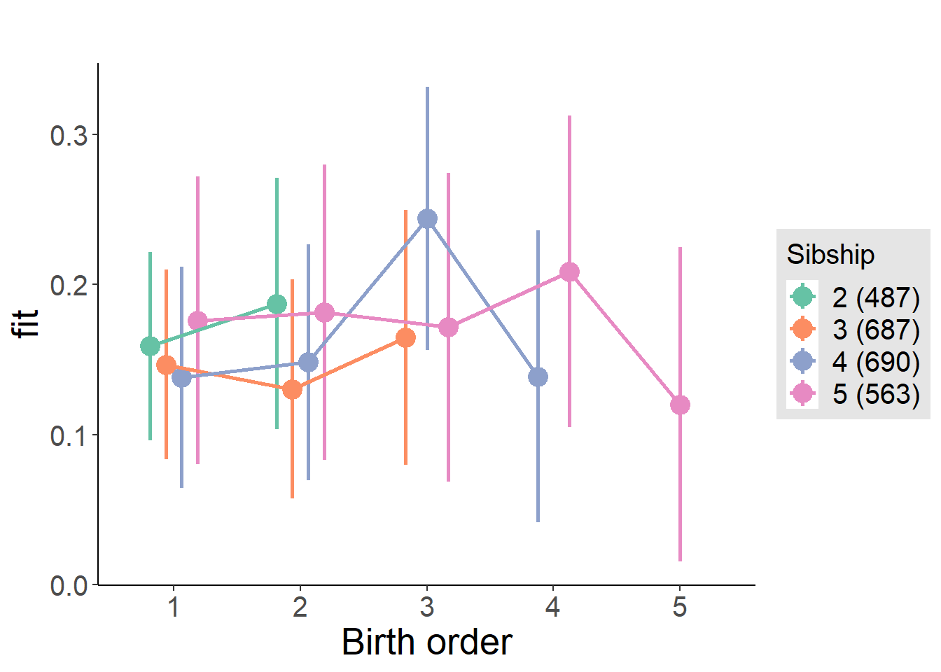
Model Comparison
###### Model 1 - Model 2
anova(m1_covariates_only, m2_birthorder_linear, m3_birthorder_nonlinear, m4_interaction)## refitting model(s) with ML (instead of REML)| Df | AIC | BIC | logLik | deviance | Chisq | Chi Df | Pr(>Chisq) |
|---|---|---|---|---|---|---|---|
| 10 | 2082 | 2140 | -1031 | 2062 | NA | NA | NA |
| 11 | 2084 | 2148 | -1031 | 2062 | 0.2536 | 1 | 0.6146 |
| 14 | 2083 | 2164 | -1028 | 2055 | 6.959 | 3 | 0.07323 |
| 20 | 2088 | 2204 | -1024 | 2048 | 6.971 | 6 | 0.3235 |
Parental full sibling order
outcome_parental_m1 <- update(m2_birthorder_linear, data = birthorder %>%
mutate(sibling_count = sibling_count_genes_factor,
birth_order_nonlinear = birthorder_genes_factor,
birth_order = birthorder_genes,
count_birth_order = count_birthorder_genes
) %>%
filter(sibling_count != "1"))
compare_models_markdown(outcome_parental_m1)Basic Model
Model Summary
m1_covariates_only <- update(m2_birthorder_linear, formula = . ~ . - birth_order)
tidy(m1_covariates_only, conf.int = T, conf.level = 0.995)| effect | group | term | estimate | std.error | statistic | df | p.value | conf.low | conf.high |
|---|---|---|---|---|---|---|---|---|---|
| fixed | NA | (Intercept) | 0.3212 | 0.3165 | 1.015 | 2636 | 0.3103 | -0.5673 | 1.21 |
| fixed | NA | poly(age, 3, raw = TRUE)1 | -0.02337 | 0.03513 | -0.6652 | 2636 | 0.506 | -0.122 | 0.07524 |
| fixed | NA | poly(age, 3, raw = TRUE)2 | 0.0009649 | 0.001247 | 0.7736 | 2636 | 0.4392 | -0.002536 | 0.004466 |
| fixed | NA | poly(age, 3, raw = TRUE)3 | -0.00001167 | 0.00001419 | -0.8222 | 2636 | 0.411 | -0.00005149 | 0.00002816 |
| fixed | NA | male | 0.0154 | 0.01468 | 1.049 | 2609 | 0.2943 | -0.0258 | 0.05659 |
| fixed | NA | sibling_count3 | -0.00634 | 0.02034 | -0.3117 | 2075 | 0.7553 | -0.06343 | 0.05075 |
| fixed | NA | sibling_count4 | -0.008444 | 0.0214 | -0.3946 | 1922 | 0.6932 | -0.0685 | 0.05162 |
| fixed | NA | sibling_count5 | 0.007433 | 0.02465 | 0.3015 | 1622 | 0.7631 | -0.06177 | 0.07664 |
| ran_pars | mother_pidlink | sd__(Intercept) | 0.1445 | NA | NA | NA | NA | NA | NA |
| ran_pars | Residual | sd__Observation | 0.345 | NA | NA | NA | NA | NA | NA |
Coefficient Plot
plot(allEffects(m1_covariates_only, confidence.level = 0.995))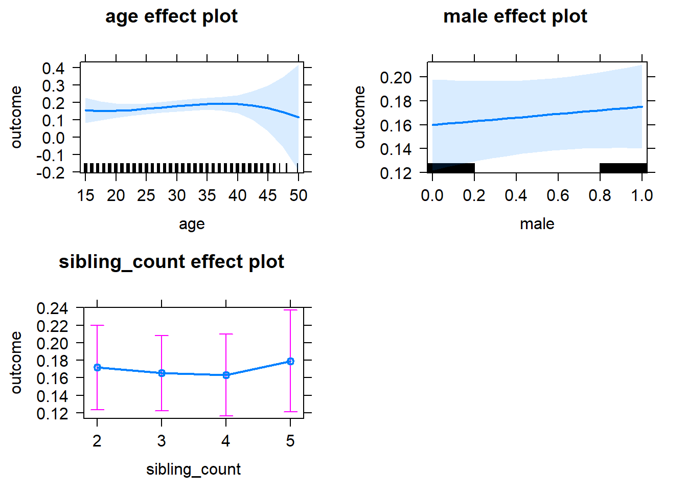
Add Birth Order Linear
Model Summary
tidy(m2_birthorder_linear, conf.int = T, conf.level = 0.995)| effect | group | term | estimate | std.error | statistic | df | p.value | conf.low | conf.high |
|---|---|---|---|---|---|---|---|---|---|
| fixed | NA | (Intercept) | 0.3206 | 0.3165 | 1.013 | 2635 | 0.3112 | -0.5679 | 1.209 |
| fixed | NA | birth_order | 0.006712 | 0.007454 | 0.9006 | 2422 | 0.3679 | -0.01421 | 0.02763 |
| fixed | NA | poly(age, 3, raw = TRUE)1 | -0.02413 | 0.03514 | -0.6866 | 2635 | 0.4924 | -0.1228 | 0.07451 |
| fixed | NA | poly(age, 3, raw = TRUE)2 | 0.000981 | 0.001247 | 0.7864 | 2635 | 0.4317 | -0.002521 | 0.004483 |
| fixed | NA | poly(age, 3, raw = TRUE)3 | -0.00001167 | 0.00001419 | -0.8227 | 2635 | 0.4108 | -0.0000515 | 0.00002815 |
| fixed | NA | male | 0.01548 | 0.01468 | 1.055 | 2608 | 0.2915 | -0.02571 | 0.05668 |
| fixed | NA | sibling_count3 | -0.009568 | 0.02065 | -0.4633 | 2108 | 0.6432 | -0.06755 | 0.04841 |
| fixed | NA | sibling_count4 | -0.01528 | 0.02271 | -0.6731 | 2054 | 0.5009 | -0.07902 | 0.04845 |
| fixed | NA | sibling_count5 | -0.00364 | 0.02755 | -0.1321 | 1910 | 0.8949 | -0.08098 | 0.0737 |
| ran_pars | mother_pidlink | sd__(Intercept) | 0.1445 | NA | NA | NA | NA | NA | NA |
| ran_pars | Residual | sd__Observation | 0.345 | NA | NA | NA | NA | NA | NA |
Coefficient Plot
plot_birthorder2(m2_birthorder_linear, separate = FALSE)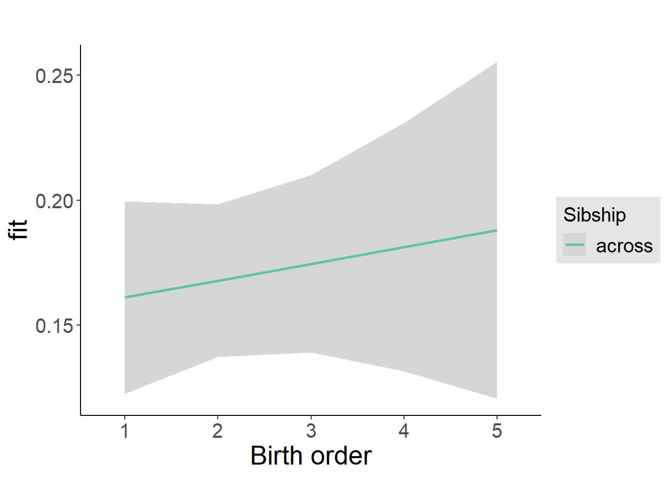
Add Birth Order Factor
Model Summary
m3_birthorder_nonlinear = update(m1_covariates_only, formula = . ~ . + birth_order_nonlinear)
tidy(m3_birthorder_nonlinear, conf.int = T, conf.level = 0.995)| effect | group | term | estimate | std.error | statistic | df | p.value | conf.low | conf.high |
|---|---|---|---|---|---|---|---|---|---|
| fixed | NA | (Intercept) | 0.2863 | 0.3169 | 0.9035 | 2631 | 0.3663 | -0.6033 | 1.176 |
| fixed | NA | poly(age, 3, raw = TRUE)1 | -0.01983 | 0.03517 | -0.5639 | 2632 | 0.5729 | -0.1185 | 0.07888 |
| fixed | NA | poly(age, 3, raw = TRUE)2 | 0.0008281 | 0.001248 | 0.6633 | 2632 | 0.5072 | -0.002676 | 0.004332 |
| fixed | NA | poly(age, 3, raw = TRUE)3 | -0.00001001 | 0.0000142 | -0.7047 | 2632 | 0.481 | -0.00004986 | 0.00002985 |
| fixed | NA | male | 0.01645 | 0.01468 | 1.12 | 2607 | 0.2626 | -0.02476 | 0.05765 |
| fixed | NA | sibling_count3 | -0.0174 | 0.02094 | -0.831 | 2168 | 0.4061 | -0.07619 | 0.04138 |
| fixed | NA | sibling_count4 | -0.02097 | 0.02297 | -0.913 | 2108 | 0.3614 | -0.08545 | 0.04351 |
| fixed | NA | sibling_count5 | 0.006 | 0.02795 | 0.2147 | 1966 | 0.83 | -0.07245 | 0.08445 |
| fixed | NA | birth_order_nonlinear2 | 0.01739 | 0.01733 | 1.004 | 2204 | 0.3157 | -0.03125 | 0.06602 |
| fixed | NA | birth_order_nonlinear3 | 0.04795 | 0.02131 | 2.25 | 2249 | 0.02453 | -0.01186 | 0.1078 |
| fixed | NA | birth_order_nonlinear4 | 0.01351 | 0.02923 | 0.4624 | 2296 | 0.6439 | -0.06853 | 0.09556 |
| fixed | NA | birth_order_nonlinear5 | -0.04285 | 0.04669 | -0.9177 | 2229 | 0.3589 | -0.1739 | 0.0882 |
| ran_pars | mother_pidlink | sd__(Intercept) | 0.1436 | NA | NA | NA | NA | NA | NA |
| ran_pars | Residual | sd__Observation | 0.3451 | NA | NA | NA | NA | NA | NA |
Coefficient Plot
plot_birthorder(m3_birthorder_nonlinear, separate = FALSE)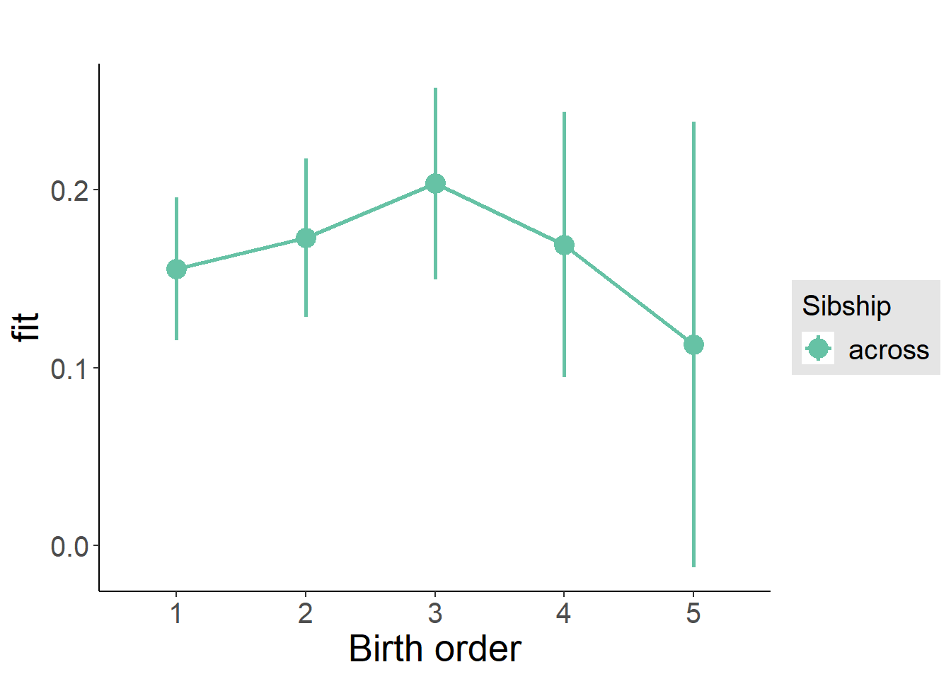
Add Interaction
Model Summary
m4_interaction = update(m3_birthorder_nonlinear, formula = . ~ . - birth_order_nonlinear - sibling_count + count_birth_order)
tidy(m4_interaction, conf.int = T, conf.level = 0.995)| effect | group | term | estimate | std.error | statistic | df | p.value | conf.low | conf.high |
|---|---|---|---|---|---|---|---|---|---|
| fixed | NA | (Intercept) | 0.2873 | 0.3172 | 0.9057 | 2624 | 0.3652 | -0.603 | 1.178 |
| fixed | NA | poly(age, 3, raw = TRUE)1 | -0.02013 | 0.0352 | -0.5718 | 2625 | 0.5675 | -0.1189 | 0.07868 |
| fixed | NA | poly(age, 3, raw = TRUE)2 | 0.000828 | 0.00125 | 0.6626 | 2625 | 0.5077 | -0.00268 | 0.004336 |
| fixed | NA | poly(age, 3, raw = TRUE)3 | -0.000009881 | 0.00001421 | -0.6951 | 2625 | 0.4871 | -0.00004978 | 0.00003002 |
| fixed | NA | male | 0.01642 | 0.0147 | 1.117 | 2602 | 0.264 | -0.02484 | 0.05768 |
| fixed | NA | count_birth_order2/2 | 0.02988 | 0.03109 | 0.9611 | 2243 | 0.3366 | -0.05739 | 0.1172 |
| fixed | NA | count_birth_order1/3 | -0.001197 | 0.02656 | -0.04507 | 2624 | 0.9641 | -0.07576 | 0.07337 |
| fixed | NA | count_birth_order2/3 | -0.007073 | 0.0295 | -0.2398 | 2628 | 0.8105 | -0.08989 | 0.07574 |
| fixed | NA | count_birth_order3/3 | 0.02579 | 0.03175 | 0.8122 | 2622 | 0.4167 | -0.06334 | 0.1149 |
| fixed | NA | count_birth_order1/4 | -0.02618 | 0.03123 | -0.8382 | 2628 | 0.402 | -0.1138 | 0.06149 |
| fixed | NA | count_birth_order2/4 | 0.01164 | 0.03273 | 0.3557 | 2623 | 0.7221 | -0.08022 | 0.1035 |
| fixed | NA | count_birth_order3/4 | 0.05322 | 0.03394 | 1.568 | 2616 | 0.117 | -0.04205 | 0.1485 |
| fixed | NA | count_birth_order4/4 | -0.03173 | 0.03683 | -0.8616 | 2611 | 0.389 | -0.1351 | 0.07165 |
| fixed | NA | count_birth_order1/5 | 0.001533 | 0.04093 | 0.03745 | 2627 | 0.9701 | -0.1134 | 0.1164 |
| fixed | NA | count_birth_order2/5 | 0.01608 | 0.0455 | 0.3534 | 2596 | 0.7238 | -0.1116 | 0.1438 |
| fixed | NA | count_birth_order3/5 | 0.03446 | 0.04429 | 0.7781 | 2593 | 0.4366 | -0.08986 | 0.1588 |
| fixed | NA | count_birth_order4/5 | 0.06496 | 0.0426 | 1.525 | 2594 | 0.1274 | -0.05461 | 0.1845 |
| fixed | NA | count_birth_order5/5 | -0.03273 | 0.04522 | -0.7239 | 2586 | 0.4692 | -0.1597 | 0.09419 |
| ran_pars | mother_pidlink | sd__(Intercept) | 0.1408 | NA | NA | NA | NA | NA | NA |
| ran_pars | Residual | sd__Observation | 0.3462 | NA | NA | NA | NA | NA | NA |
Coefficient Plot
plot_birthorder(m4_interaction)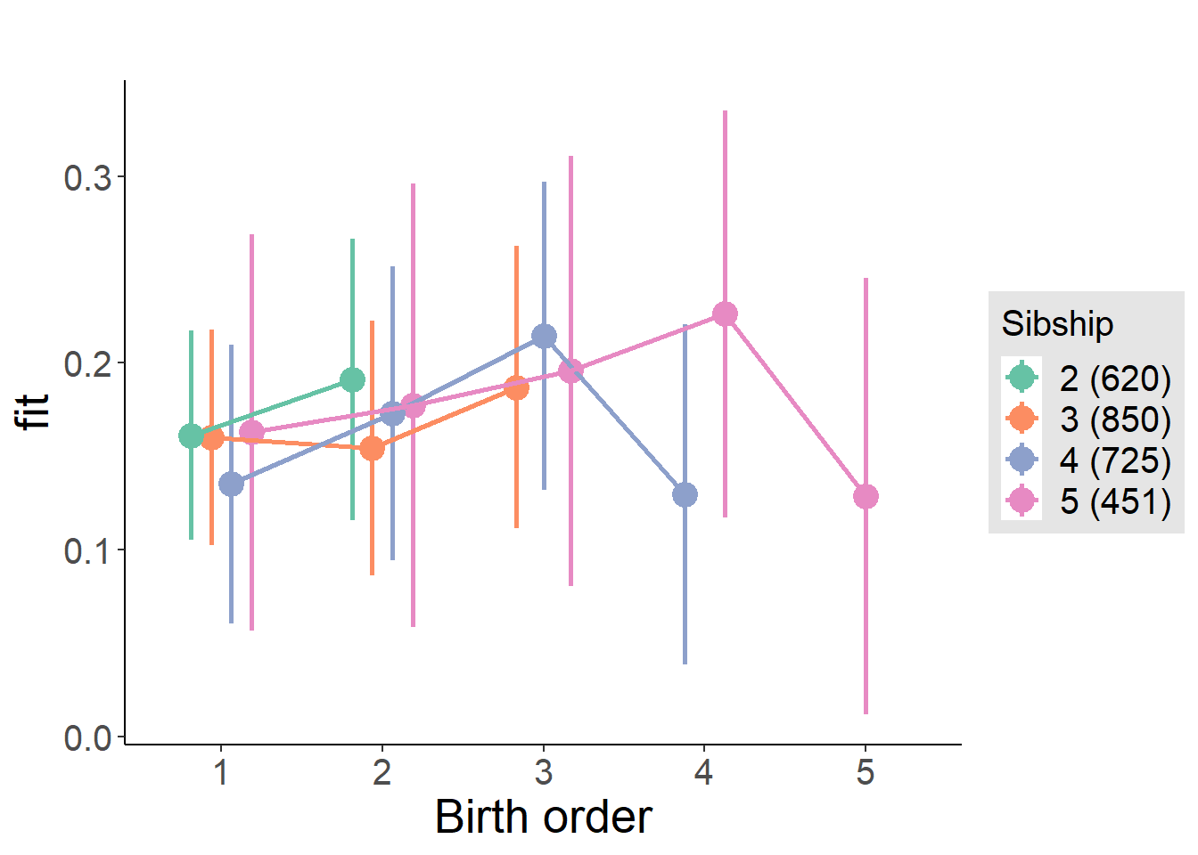
Model Comparison
###### Model 1 - Model 2
anova(m1_covariates_only, m2_birthorder_linear, m3_birthorder_nonlinear, m4_interaction)## refitting model(s) with ML (instead of REML)| Df | AIC | BIC | logLik | deviance | Chisq | Chi Df | Pr(>Chisq) |
|---|---|---|---|---|---|---|---|
| 10 | 2298 | 2357 | -1139 | 2278 | NA | NA | NA |
| 11 | 2299 | 2364 | -1139 | 2277 | 0.813 | 1 | 0.3672 |
| 14 | 2299 | 2381 | -1136 | 2271 | 6.307 | 3 | 0.09758 |
| 20 | 2307 | 2424 | -1133 | 2267 | 4.482 | 6 | 0.6118 |
Compare birth order specifications
library(coefplot)
multiplot(outcome_naive_m1, outcome_preg_m1, outcome_uterus_m1, outcome_parental_m1, dodgeHeight = 0.6,
intercept = FALSE)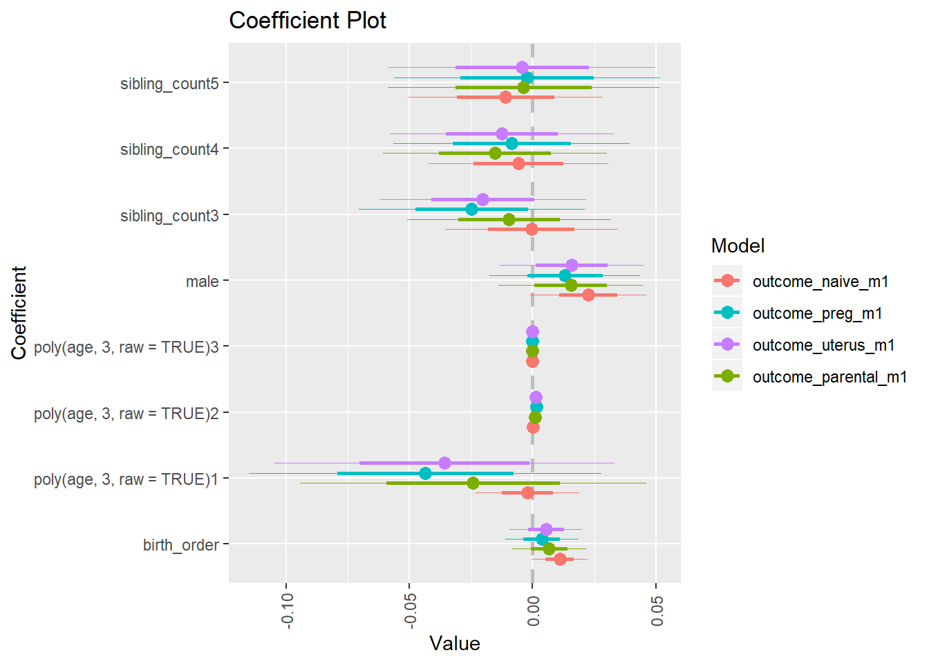
Sector_Construction
birthorder <- birthorder %>% mutate(outcome = `Sector_Construction`)
model = lmer(outcome ~ birth_order + poly(age, 3, raw = TRUE) + male + sibling_count + (1 | mother_pidlink),
data = birthorder)## boundary (singular) fit: see ?isSingularcompare_birthorder_specs(model)Naive birth order
outcome_naive_m1 <- update(m2_birthorder_linear, data = birthorder %>%
mutate(sibling_count = sibling_count_naive_factor,
birth_order_nonlinear = birthorder_naive_factor,
birth_order = birthorder_naive,
count_birth_order = count_birthorder_naive) %>%
filter(sibling_count != "1"))## boundary (singular) fit: see ?isSingularcompare_models_markdown(outcome_naive_m1)Basic Model
Model Summary
m1_covariates_only <- update(m2_birthorder_linear, formula = . ~ . - birth_order)## boundary (singular) fit: see ?isSingulartidy(m1_covariates_only, conf.int = T, conf.level = 0.995)| effect | group | term | estimate | std.error | statistic | df | p.value | conf.low | conf.high |
|---|---|---|---|---|---|---|---|---|---|
| fixed | NA | (Intercept) | 0.001036 | 0.01029 | 0.1007 | 4635 | 0.9198 | -0.02785 | 0.02992 |
| fixed | NA | poly(age, 3, raw = TRUE)1 | -0.00001562 | 0.0009133 | -0.0171 | 4635 | 0.9864 | -0.002579 | 0.002548 |
| fixed | NA | poly(age, 3, raw = TRUE)2 | 0.0000002511 | 0.00002523 | 0.009951 | 4635 | 0.9921 | -0.00007057 | 0.00007107 |
| fixed | NA | poly(age, 3, raw = TRUE)3 | 0.000000002046 | 0.0000002196 | 0.009316 | 4635 | 0.9926 | -0.0000006143 | 0.0000006184 |
| fixed | NA | male | 0.0014 | 0.001066 | 1.313 | 4635 | 0.1893 | -0.001593 | 0.004393 |
| fixed | NA | sibling_count3 | -0.001717 | 0.001486 | -1.155 | 4635 | 0.248 | -0.005888 | 0.002454 |
| fixed | NA | sibling_count4 | 0.0007807 | 0.001496 | 0.5218 | 4635 | 0.6018 | -0.003419 | 0.004981 |
| fixed | NA | sibling_count5 | -0.0007588 | 0.00155 | -0.4896 | 4635 | 0.6244 | -0.005109 | 0.003592 |
| ran_pars | mother_pidlink | sd__(Intercept) | 0 | NA | NA | NA | NA | NA | NA |
| ran_pars | Residual | sd__Observation | 0.03594 | NA | NA | NA | NA | NA | NA |
Coefficient Plot
plot(allEffects(m1_covariates_only, confidence.level = 0.995))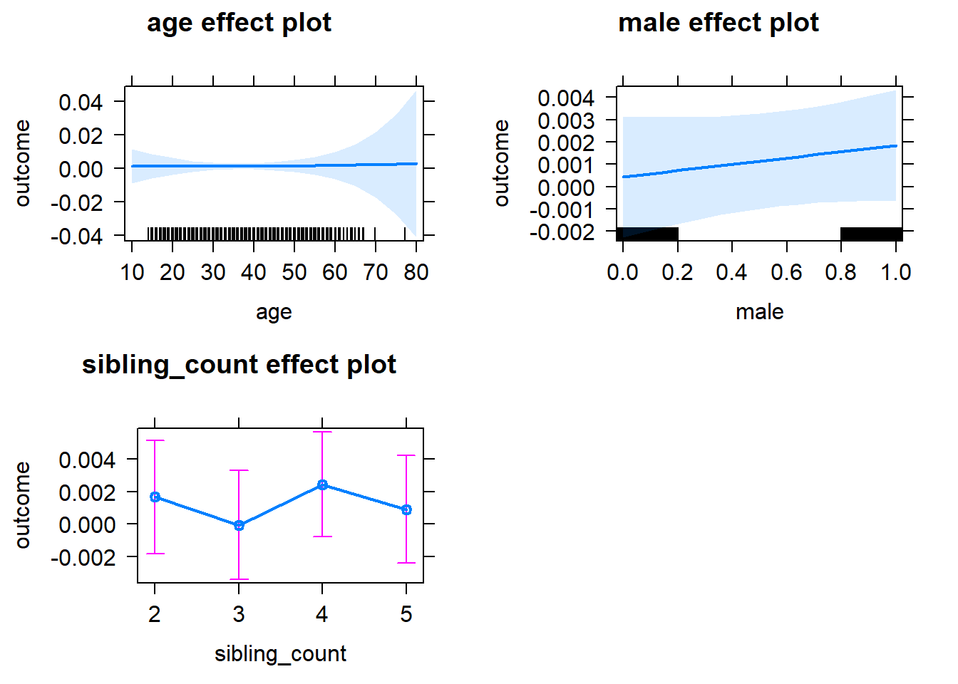
Add Birth Order Linear
Model Summary
tidy(m2_birthorder_linear, conf.int = T, conf.level = 0.995)| effect | group | term | estimate | std.error | statistic | df | p.value | conf.low | conf.high |
|---|---|---|---|---|---|---|---|---|---|
| fixed | NA | (Intercept) | 0.0008323 | 0.01029 | 0.08088 | 4634 | 0.9355 | -0.02805 | 0.02972 |
| fixed | NA | birth_order | -0.0007178 | 0.000531 | -1.352 | 4634 | 0.1765 | -0.002208 | 0.0007727 |
| fixed | NA | poly(age, 3, raw = TRUE)1 | 0.00009303 | 0.0009168 | 0.1015 | 4634 | 0.9192 | -0.00248 | 0.002666 |
| fixed | NA | poly(age, 3, raw = TRUE)2 | -0.000002422 | 0.0000253 | -0.09571 | 4634 | 0.9238 | -0.00007345 | 0.00006861 |
| fixed | NA | poly(age, 3, raw = TRUE)3 | 0.00000002 | 0.00000022 | 0.09094 | 4634 | 0.9275 | -0.0000005974 | 0.0000006375 |
| fixed | NA | male | 0.001391 | 0.001066 | 1.304 | 4634 | 0.1922 | -0.001602 | 0.004384 |
| fixed | NA | sibling_count3 | -0.001439 | 0.0015 | -0.9591 | 4634 | 0.3375 | -0.005649 | 0.002772 |
| fixed | NA | sibling_count4 | 0.001377 | 0.00156 | 0.8827 | 4634 | 0.3774 | -0.003001 | 0.005755 |
| fixed | NA | sibling_count5 | 0.0001781 | 0.001698 | 0.1049 | 4634 | 0.9165 | -0.004587 | 0.004943 |
| ran_pars | mother_pidlink | sd__(Intercept) | 0 | NA | NA | NA | NA | NA | NA |
| ran_pars | Residual | sd__Observation | 0.03593 | NA | NA | NA | NA | NA | NA |
Coefficient Plot
plot_birthorder2(m2_birthorder_linear, separate = FALSE)
Add Birth Order Factor
Model Summary
m3_birthorder_nonlinear = update(m1_covariates_only, formula = . ~ . + birth_order_nonlinear)## boundary (singular) fit: see ?isSingulartidy(m3_birthorder_nonlinear, conf.int = T, conf.level = 0.995)| effect | group | term | estimate | std.error | statistic | df | p.value | conf.low | conf.high |
|---|---|---|---|---|---|---|---|---|---|
| fixed | NA | (Intercept) | -0.0005132 | 0.01033 | -0.0497 | 4631 | 0.9604 | -0.0295 | 0.02847 |
| fixed | NA | poly(age, 3, raw = TRUE)1 | 0.0001149 | 0.0009171 | 0.1252 | 4631 | 0.9003 | -0.00246 | 0.002689 |
| fixed | NA | poly(age, 3, raw = TRUE)2 | -0.000003243 | 0.00002532 | -0.1281 | 4631 | 0.8981 | -0.00007431 | 0.00006783 |
| fixed | NA | poly(age, 3, raw = TRUE)3 | 0.00000002885 | 0.0000002202 | 0.131 | 4631 | 0.8958 | -0.0000005892 | 0.0000006468 |
| fixed | NA | male | 0.001379 | 0.001067 | 1.293 | 4631 | 0.1962 | -0.001615 | 0.004373 |
| fixed | NA | sibling_count3 | -0.001281 | 0.001529 | -0.8377 | 4631 | 0.4022 | -0.005574 | 0.003012 |
| fixed | NA | sibling_count4 | 0.001694 | 0.001592 | 1.064 | 4631 | 0.2874 | -0.002775 | 0.006164 |
| fixed | NA | sibling_count5 | 0.000358 | 0.001717 | 0.2084 | 4631 | 0.8349 | -0.004463 | 0.005179 |
| fixed | NA | birth_order_nonlinear2 | 0.0005383 | 0.001283 | 0.4196 | 4631 | 0.6748 | -0.003062 | 0.004139 |
| fixed | NA | birth_order_nonlinear3 | -0.001747 | 0.001626 | -1.074 | 4631 | 0.2827 | -0.006313 | 0.002818 |
| fixed | NA | birth_order_nonlinear4 | -0.002672 | 0.002125 | -1.257 | 4631 | 0.2087 | -0.008637 | 0.003293 |
| fixed | NA | birth_order_nonlinear5 | -0.00185 | 0.003064 | -0.6037 | 4631 | 0.5461 | -0.01045 | 0.006751 |
| ran_pars | mother_pidlink | sd__(Intercept) | 0 | NA | NA | NA | NA | NA | NA |
| ran_pars | Residual | sd__Observation | 0.03594 | NA | NA | NA | NA | NA | NA |
Coefficient Plot
plot_birthorder(m3_birthorder_nonlinear, separate = FALSE)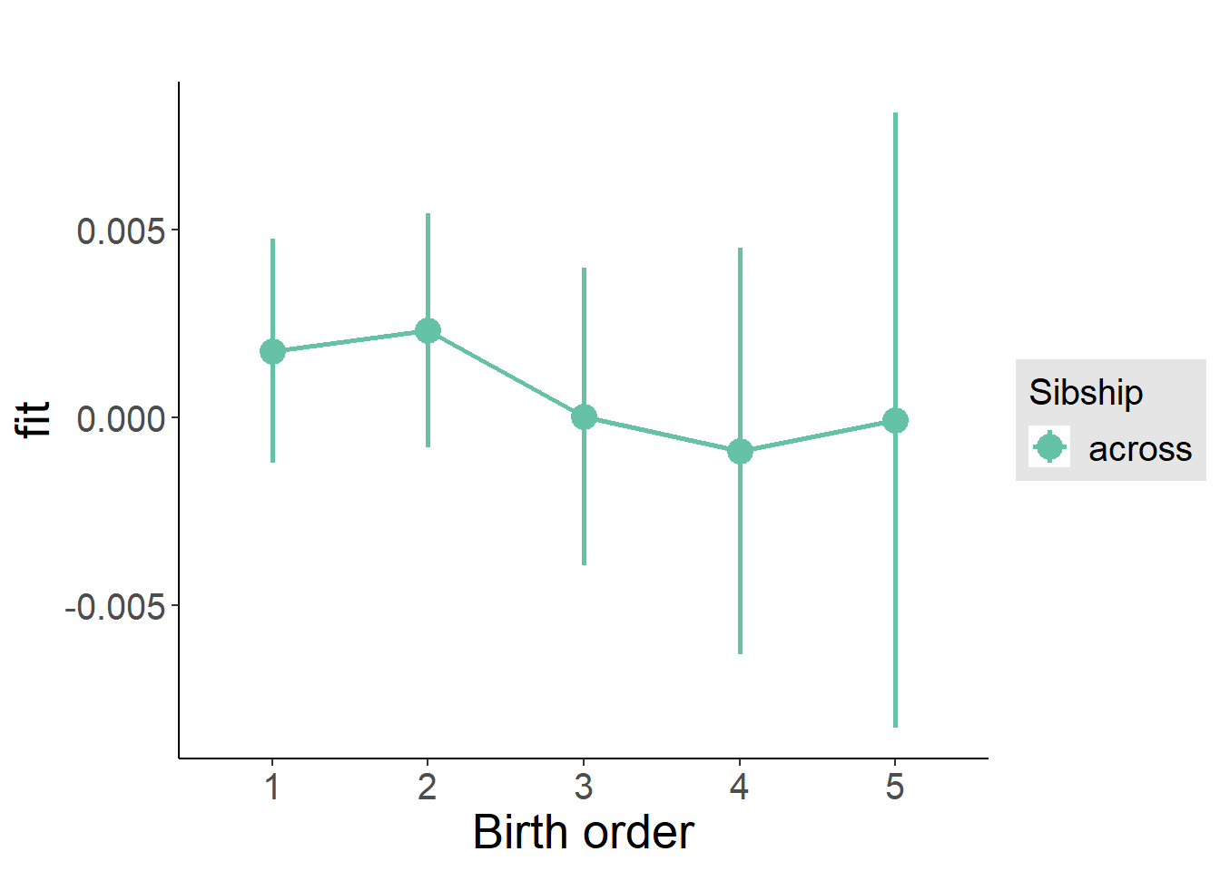
Add Interaction
Model Summary
m4_interaction = update(m3_birthorder_nonlinear, formula = . ~ . - birth_order_nonlinear - sibling_count + count_birth_order)## boundary (singular) fit: see ?isSingulartidy(m4_interaction, conf.int = T, conf.level = 0.995)| effect | group | term | estimate | std.error | statistic | df | p.value | conf.low | conf.high |
|---|---|---|---|---|---|---|---|---|---|
| fixed | NA | (Intercept) | -0.0001367 | 0.01035 | -0.01321 | 4625 | 0.9895 | -0.02918 | 0.02891 |
| fixed | NA | poly(age, 3, raw = TRUE)1 | 0.00007536 | 0.0009182 | 0.08207 | 4625 | 0.9346 | -0.002502 | 0.002653 |
| fixed | NA | poly(age, 3, raw = TRUE)2 | -0.00000237 | 0.00002534 | -0.09355 | 4625 | 0.9255 | -0.0000735 | 0.00006876 |
| fixed | NA | poly(age, 3, raw = TRUE)3 | 0.00000002363 | 0.0000002203 | 0.1073 | 4625 | 0.9146 | -0.0000005947 | 0.0000006419 |
| fixed | NA | male | 0.001365 | 0.001067 | 1.279 | 4625 | 0.2011 | -0.001631 | 0.004361 |
| fixed | NA | count_birth_order2/2 | 0.0008685 | 0.002187 | 0.3972 | 4625 | 0.6912 | -0.005269 | 0.007006 |
| fixed | NA | count_birth_order1/3 | -0.001391 | 0.002061 | -0.6751 | 4625 | 0.4996 | -0.007176 | 0.004393 |
| fixed | NA | count_birth_order2/3 | -0.001409 | 0.002295 | -0.614 | 4625 | 0.5392 | -0.00785 | 0.005032 |
| fixed | NA | count_birth_order3/3 | -0.001426 | 0.002525 | -0.5648 | 4625 | 0.5722 | -0.008513 | 0.005661 |
| fixed | NA | count_birth_order1/4 | 0.00372 | 0.002271 | 1.638 | 4625 | 0.1016 | -0.002656 | 0.01009 |
| fixed | NA | count_birth_order2/4 | 0.001717 | 0.002437 | 0.7045 | 4625 | 0.4811 | -0.005123 | 0.008556 |
| fixed | NA | count_birth_order3/4 | -0.001372 | 0.002572 | -0.5335 | 4625 | 0.5937 | -0.008591 | 0.005847 |
| fixed | NA | count_birth_order4/4 | -0.001397 | 0.002773 | -0.5038 | 4625 | 0.6144 | -0.00918 | 0.006386 |
| fixed | NA | count_birth_order1/5 | -0.001436 | 0.002563 | -0.5605 | 4625 | 0.5752 | -0.008631 | 0.005758 |
| fixed | NA | count_birth_order2/5 | 0.002839 | 0.002724 | 1.042 | 4625 | 0.2973 | -0.004807 | 0.01048 |
| fixed | NA | count_birth_order3/5 | -0.001355 | 0.002866 | -0.4728 | 4625 | 0.6363 | -0.0094 | 0.00669 |
| fixed | NA | count_birth_order4/5 | -0.00145 | 0.003029 | -0.4787 | 4625 | 0.6322 | -0.009952 | 0.007052 |
| fixed | NA | count_birth_order5/5 | -0.001345 | 0.003035 | -0.4431 | 4625 | 0.6577 | -0.009864 | 0.007174 |
| ran_pars | mother_pidlink | sd__(Intercept) | 0 | NA | NA | NA | NA | NA | NA |
| ran_pars | Residual | sd__Observation | 0.03595 | NA | NA | NA | NA | NA | NA |
Coefficient Plot
plot_birthorder(m4_interaction)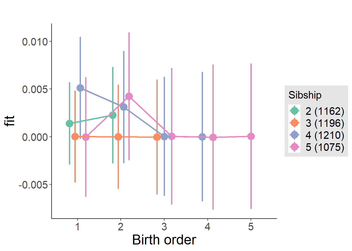
Model Comparison
###### Model 1 - Model 2
anova(m1_covariates_only, m2_birthorder_linear, m3_birthorder_nonlinear, m4_interaction)## refitting model(s) with ML (instead of REML)| Df | AIC | BIC | logLik | deviance | Chisq | Chi Df | Pr(>Chisq) |
|---|---|---|---|---|---|---|---|
| 10 | -17697 | -17632 | 8858 | -17717 | NA | NA | NA |
| 11 | -17697 | -17626 | 8859 | -17719 | 1.831 | 1 | 0.1761 |
| 14 | -17692 | -17602 | 8860 | -17720 | 1.564 | 3 | 0.6675 |
| 20 | -17684 | -17555 | 8862 | -17724 | 3.873 | 6 | 0.6938 |
Maternal birth order
outcome_uterus_m1 <- update(m2_birthorder_linear, data = birthorder %>%
mutate(sibling_count = sibling_count_uterus_alive_factor,
birth_order_nonlinear = birthorder_uterus_alive_factor,
birth_order = birthorder_uterus_alive,
count_birth_order = count_birthorder_uterus_alive) %>%
filter(sibling_count != "1"))## boundary (singular) fit: see ?isSingularcompare_models_markdown(outcome_uterus_m1)Basic Model
Model Summary
m1_covariates_only <- update(m2_birthorder_linear, formula = . ~ . - birth_order)## boundary (singular) fit: see ?isSingulartidy(m1_covariates_only, conf.int = T, conf.level = 0.995)| effect | group | term | estimate | std.error | statistic | df | p.value | conf.low | conf.high |
|---|---|---|---|---|---|---|---|---|---|
| fixed | NA | (Intercept) | -0.01011 | 0.03261 | -0.31 | 2634 | 0.7565 | -0.1017 | 0.08143 |
| fixed | NA | poly(age, 3, raw = TRUE)1 | 0.001089 | 0.003609 | 0.3018 | 2634 | 0.7628 | -0.009041 | 0.01122 |
| fixed | NA | poly(age, 3, raw = TRUE)2 | -0.00002568 | 0.0001278 | -0.2009 | 2634 | 0.8408 | -0.0003845 | 0.0003331 |
| fixed | NA | poly(age, 3, raw = TRUE)3 | 0.0000001472 | 0.00000145 | 0.1016 | 2634 | 0.9191 | -0.000003922 | 0.000004217 |
| fixed | NA | male | 0.001146 | 0.001537 | 0.7457 | 2634 | 0.4559 | -0.003169 | 0.005461 |
| fixed | NA | sibling_count3 | -0.002189 | 0.002107 | -1.039 | 2634 | 0.2989 | -0.008104 | 0.003725 |
| fixed | NA | sibling_count4 | -0.003388 | 0.002173 | -1.559 | 2634 | 0.1191 | -0.009488 | 0.002712 |
| fixed | NA | sibling_count5 | -0.001382 | 0.00241 | -0.5736 | 2634 | 0.5663 | -0.008146 | 0.005382 |
| ran_pars | mother_pidlink | sd__(Intercept) | 0 | NA | NA | NA | NA | NA | NA |
| ran_pars | Residual | sd__Observation | 0.03891 | NA | NA | NA | NA | NA | NA |
Coefficient Plot
plot(allEffects(m1_covariates_only, confidence.level = 0.995))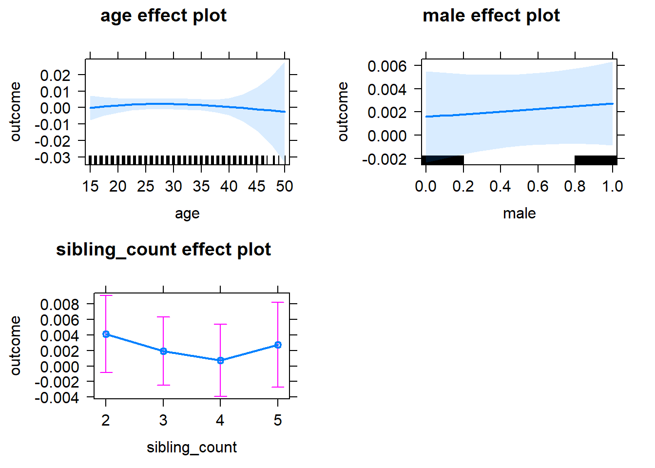
Add Birth Order Linear
Model Summary
tidy(m2_birthorder_linear, conf.int = T, conf.level = 0.995)| effect | group | term | estimate | std.error | statistic | df | p.value | conf.low | conf.high |
|---|---|---|---|---|---|---|---|---|---|
| fixed | NA | (Intercept) | -0.009762 | 0.0326 | -0.2995 | 2633 | 0.7646 | -0.1013 | 0.08174 |
| fixed | NA | birth_order | -0.001465 | 0.0007791 | -1.881 | 2633 | 0.06009 | -0.003652 | 0.0007215 |
| fixed | NA | poly(age, 3, raw = TRUE)1 | 0.001218 | 0.003608 | 0.3375 | 2633 | 0.7358 | -0.00891 | 0.01134 |
| fixed | NA | poly(age, 3, raw = TRUE)2 | -0.0000277 | 0.0001278 | -0.2168 | 2633 | 0.8284 | -0.0003863 | 0.0003309 |
| fixed | NA | poly(age, 3, raw = TRUE)3 | 0.0000001336 | 0.000001449 | 0.0922 | 2633 | 0.9265 | -0.000003934 | 0.000004201 |
| fixed | NA | male | 0.001142 | 0.001536 | 0.743 | 2633 | 0.4576 | -0.003171 | 0.005455 |
| fixed | NA | sibling_count3 | -0.001498 | 0.002138 | -0.7008 | 2633 | 0.4835 | -0.007499 | 0.004503 |
| fixed | NA | sibling_count4 | -0.001896 | 0.002312 | -0.8198 | 2633 | 0.4124 | -0.008386 | 0.004595 |
| fixed | NA | sibling_count5 | 0.001111 | 0.002749 | 0.4042 | 2633 | 0.6861 | -0.006606 | 0.008828 |
| ran_pars | mother_pidlink | sd__(Intercept) | 0 | NA | NA | NA | NA | NA | NA |
| ran_pars | Residual | sd__Observation | 0.03889 | NA | NA | NA | NA | NA | NA |
Coefficient Plot
plot_birthorder2(m2_birthorder_linear, separate = FALSE)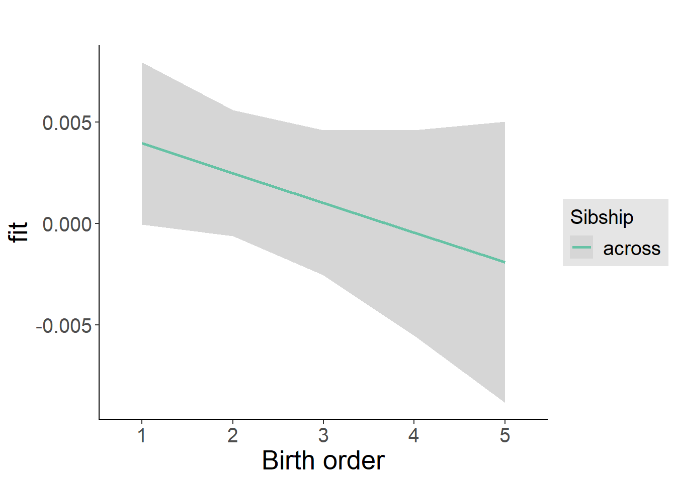
Add Birth Order Factor
Model Summary
m3_birthorder_nonlinear = update(m1_covariates_only, formula = . ~ . + birth_order_nonlinear)## boundary (singular) fit: see ?isSingulartidy(m3_birthorder_nonlinear, conf.int = T, conf.level = 0.995)| effect | group | term | estimate | std.error | statistic | df | p.value | conf.low | conf.high |
|---|---|---|---|---|---|---|---|---|---|
| fixed | NA | (Intercept) | -0.009893 | 0.03267 | -0.3028 | 2630 | 0.762 | -0.1016 | 0.0818 |
| fixed | NA | poly(age, 3, raw = TRUE)1 | 0.001136 | 0.003614 | 0.3143 | 2630 | 0.7533 | -0.009009 | 0.01128 |
| fixed | NA | poly(age, 3, raw = TRUE)2 | -0.00002449 | 0.000128 | -0.1914 | 2630 | 0.8482 | -0.0003837 | 0.0003347 |
| fixed | NA | poly(age, 3, raw = TRUE)3 | 0.00000009634 | 0.000001451 | 0.06638 | 2630 | 0.9471 | -0.000003978 | 0.00000417 |
| fixed | NA | male | 0.001101 | 0.001538 | 0.7162 | 2630 | 0.474 | -0.003216 | 0.005418 |
| fixed | NA | sibling_count3 | -0.001443 | 0.002173 | -0.6642 | 2630 | 0.5066 | -0.007542 | 0.004656 |
| fixed | NA | sibling_count4 | -0.002054 | 0.002346 | -0.8755 | 2630 | 0.3814 | -0.008641 | 0.004532 |
| fixed | NA | sibling_count5 | 0.0006755 | 0.002786 | 0.2424 | 2630 | 0.8085 | -0.007146 | 0.008497 |
| fixed | NA | birth_order_nonlinear2 | -0.003604 | 0.00187 | -1.927 | 2630 | 0.05408 | -0.008854 | 0.001646 |
| fixed | NA | birth_order_nonlinear3 | -0.003351 | 0.002277 | -1.471 | 2630 | 0.1413 | -0.009743 | 0.003042 |
| fixed | NA | birth_order_nonlinear4 | -0.003911 | 0.003028 | -1.292 | 2630 | 0.1966 | -0.01241 | 0.004588 |
| fixed | NA | birth_order_nonlinear5 | -0.005469 | 0.004696 | -1.165 | 2630 | 0.2443 | -0.01865 | 0.007714 |
| ran_pars | mother_pidlink | sd__(Intercept) | 0.0000000007183 | NA | NA | NA | NA | NA | NA |
| ran_pars | Residual | sd__Observation | 0.0389 | NA | NA | NA | NA | NA | NA |
Coefficient Plot
plot_birthorder(m3_birthorder_nonlinear, separate = FALSE)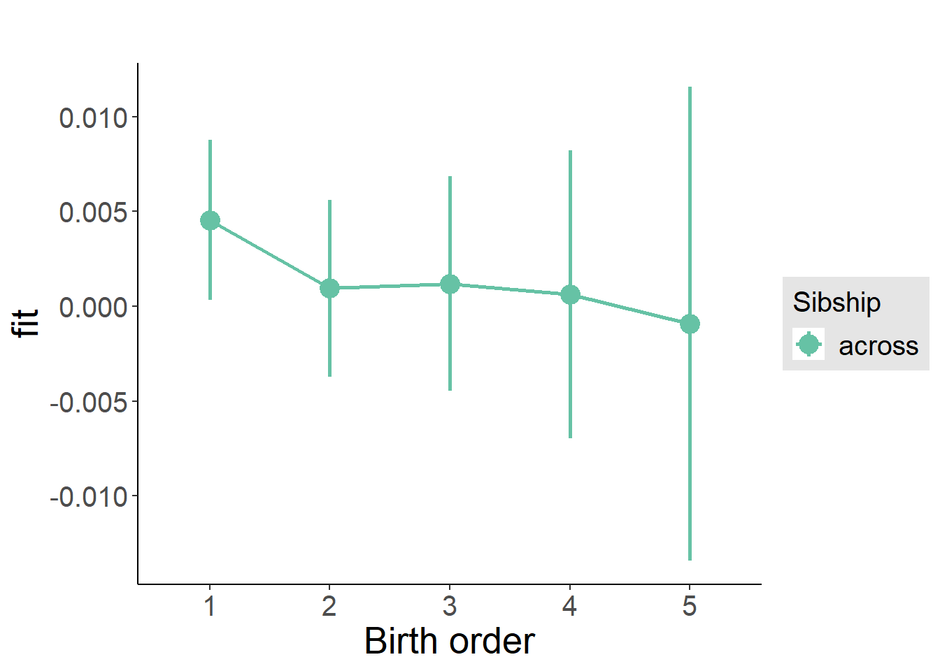
Add Interaction
Model Summary
m4_interaction = update(m3_birthorder_nonlinear, formula = . ~ . - birth_order_nonlinear - sibling_count + count_birth_order)## boundary (singular) fit: see ?isSingulartidy(m4_interaction, conf.int = T, conf.level = 0.995)| effect | group | term | estimate | std.error | statistic | df | p.value | conf.low | conf.high |
|---|---|---|---|---|---|---|---|---|---|
| fixed | NA | (Intercept) | -0.008155 | 0.0327 | -0.2494 | 2624 | 0.8031 | -0.09995 | 0.08364 |
| fixed | NA | poly(age, 3, raw = TRUE)1 | 0.0009659 | 0.003618 | 0.267 | 2624 | 0.7895 | -0.00919 | 0.01112 |
| fixed | NA | poly(age, 3, raw = TRUE)2 | -0.00001708 | 0.0001281 | -0.1333 | 2624 | 0.8939 | -0.0003768 | 0.0003426 |
| fixed | NA | poly(age, 3, raw = TRUE)3 | -0.000000002605 | 0.000001453 | -0.001792 | 2624 | 0.9986 | -0.000004082 | 0.000004077 |
| fixed | NA | male | 0.001071 | 0.001541 | 0.6952 | 2624 | 0.487 | -0.003253 | 0.005395 |
| fixed | NA | count_birth_order2/2 | -0.00524 | 0.003411 | -1.536 | 2624 | 0.1246 | -0.01481 | 0.004335 |
| fixed | NA | count_birth_order1/3 | -0.002433 | 0.002821 | -0.8625 | 2624 | 0.3885 | -0.01035 | 0.005486 |
| fixed | NA | count_birth_order2/3 | -0.005071 | 0.003136 | -1.617 | 2624 | 0.106 | -0.01387 | 0.003733 |
| fixed | NA | count_birth_order3/3 | -0.005146 | 0.003419 | -1.505 | 2624 | 0.1324 | -0.01474 | 0.004451 |
| fixed | NA | count_birth_order1/4 | -0.004864 | 0.003245 | -1.499 | 2624 | 0.1341 | -0.01397 | 0.004246 |
| fixed | NA | count_birth_order2/4 | -0.005094 | 0.003437 | -1.482 | 2624 | 0.1384 | -0.01474 | 0.004554 |
| fixed | NA | count_birth_order3/4 | -0.005095 | 0.003566 | -1.429 | 2624 | 0.1532 | -0.0151 | 0.004914 |
| fixed | NA | count_birth_order4/4 | -0.005329 | 0.003812 | -1.398 | 2624 | 0.1623 | -0.01603 | 0.005372 |
| fixed | NA | count_birth_order1/5 | 0.004688 | 0.004286 | 1.094 | 2624 | 0.2742 | -0.007342 | 0.01672 |
| fixed | NA | count_birth_order2/5 | -0.004959 | 0.004614 | -1.075 | 2624 | 0.2825 | -0.01791 | 0.007992 |
| fixed | NA | count_birth_order3/5 | -0.005094 | 0.004383 | -1.162 | 2624 | 0.2452 | -0.0174 | 0.007208 |
| fixed | NA | count_birth_order4/5 | -0.005384 | 0.004272 | -1.26 | 2624 | 0.2077 | -0.01738 | 0.006608 |
| fixed | NA | count_birth_order5/5 | -0.005355 | 0.004495 | -1.191 | 2624 | 0.2336 | -0.01797 | 0.007263 |
| ran_pars | mother_pidlink | sd__(Intercept) | 0 | NA | NA | NA | NA | NA | NA |
| ran_pars | Residual | sd__Observation | 0.03892 | NA | NA | NA | NA | NA | NA |
Coefficient Plot
plot_birthorder(m4_interaction)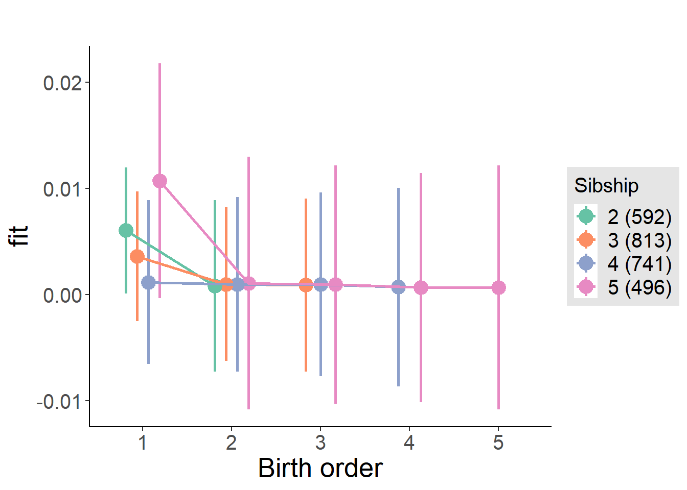
Model Comparison
###### Model 1 - Model 2
anova(m1_covariates_only, m2_birthorder_linear, m3_birthorder_nonlinear, m4_interaction)## refitting model(s) with ML (instead of REML)| Df | AIC | BIC | logLik | deviance | Chisq | Chi Df | Pr(>Chisq) |
|---|---|---|---|---|---|---|---|
| 10 | -9645 | -9586 | 4832 | -9665 | NA | NA | NA |
| 11 | -9647 | -9582 | 4834 | -9669 | 3.548 | 1 | 0.05963 |
| 14 | -9642 | -9560 | 4835 | -9670 | 1.618 | 3 | 0.6553 |
| 20 | -9634 | -9516 | 4837 | -9674 | 3.518 | 6 | 0.7416 |
Maternal pregnancy order
outcome_preg_m1 <- update(m2_birthorder_linear, data = birthorder %>%
mutate(sibling_count = sibling_count_uterus_preg_factor,
birth_order_nonlinear = birthorder_uterus_preg_factor,
birth_order = birthorder_uterus_preg,
count_birth_order = count_birthorder_uterus_preg
) %>%
filter(sibling_count != "1"))## boundary (singular) fit: see ?isSingularcompare_models_markdown(outcome_preg_m1)Basic Model
Model Summary
m1_covariates_only <- update(m2_birthorder_linear, formula = . ~ . - birth_order)## boundary (singular) fit: see ?isSingulartidy(m1_covariates_only, conf.int = T, conf.level = 0.995)| effect | group | term | estimate | std.error | statistic | df | p.value | conf.low | conf.high |
|---|---|---|---|---|---|---|---|---|---|
| fixed | NA | (Intercept) | -0.01089 | 0.03525 | -0.3091 | 2419 | 0.7573 | -0.1098 | 0.08805 |
| fixed | NA | poly(age, 3, raw = TRUE)1 | 0.001186 | 0.003903 | 0.3038 | 2419 | 0.7613 | -0.00977 | 0.01214 |
| fixed | NA | poly(age, 3, raw = TRUE)2 | -0.00002695 | 0.0001382 | -0.1949 | 2419 | 0.8455 | -0.000415 | 0.0003611 |
| fixed | NA | poly(age, 3, raw = TRUE)3 | 0.0000001427 | 0.000001568 | 0.09099 | 2419 | 0.9275 | -0.000004259 | 0.000004545 |
| fixed | NA | male | 0.001312 | 0.001674 | 0.7836 | 2419 | 0.4333 | -0.003387 | 0.00601 |
| fixed | NA | sibling_count3 | -0.00277 | 0.002413 | -1.148 | 2419 | 0.2511 | -0.009544 | 0.004004 |
| fixed | NA | sibling_count4 | -0.004254 | 0.002437 | -1.746 | 2419 | 0.08093 | -0.01109 | 0.002585 |
| fixed | NA | sibling_count5 | -0.002457 | 0.00256 | -0.9595 | 2419 | 0.3374 | -0.009644 | 0.00473 |
| ran_pars | mother_pidlink | sd__(Intercept) | 0 | NA | NA | NA | NA | NA | NA |
| ran_pars | Residual | sd__Observation | 0.04059 | NA | NA | NA | NA | NA | NA |
Coefficient Plot
plot(allEffects(m1_covariates_only, confidence.level = 0.995))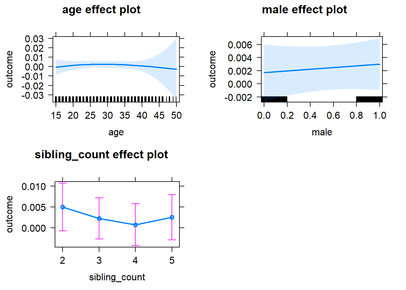
Add Birth Order Linear
Model Summary
tidy(m2_birthorder_linear, conf.int = T, conf.level = 0.995)| effect | group | term | estimate | std.error | statistic | df | p.value | conf.low | conf.high |
|---|---|---|---|---|---|---|---|---|---|
| fixed | NA | (Intercept) | -0.009765 | 0.03524 | -0.2771 | 2418 | 0.7817 | -0.1087 | 0.08915 |
| fixed | NA | birth_order | -0.001436 | 0.0008233 | -1.745 | 2418 | 0.08116 | -0.003747 | 0.0008745 |
| fixed | NA | poly(age, 3, raw = TRUE)1 | 0.001244 | 0.003902 | 0.3189 | 2418 | 0.7498 | -0.009708 | 0.0122 |
| fixed | NA | poly(age, 3, raw = TRUE)2 | -0.00002709 | 0.0001382 | -0.196 | 2418 | 0.8446 | -0.000415 | 0.0003608 |
| fixed | NA | poly(age, 3, raw = TRUE)3 | 0.0000001131 | 0.000001568 | 0.07217 | 2418 | 0.9425 | -0.000004287 | 0.000004513 |
| fixed | NA | male | 0.001269 | 0.001673 | 0.7584 | 2418 | 0.4483 | -0.003428 | 0.005966 |
| fixed | NA | sibling_count3 | -0.002089 | 0.002444 | -0.8549 | 2418 | 0.3927 | -0.008948 | 0.00477 |
| fixed | NA | sibling_count4 | -0.002906 | 0.002555 | -1.137 | 2418 | 0.2556 | -0.01008 | 0.004267 |
| fixed | NA | sibling_count5 | -0.0001687 | 0.002876 | -0.05865 | 2418 | 0.9532 | -0.008241 | 0.007903 |
| ran_pars | mother_pidlink | sd__(Intercept) | 0 | NA | NA | NA | NA | NA | NA |
| ran_pars | Residual | sd__Observation | 0.04057 | NA | NA | NA | NA | NA | NA |
Coefficient Plot
plot_birthorder2(m2_birthorder_linear, separate = FALSE)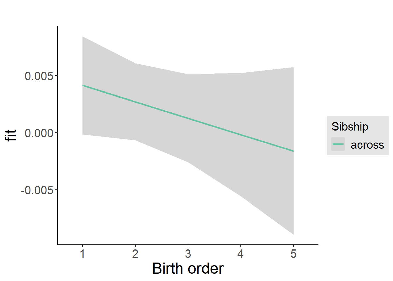
Add Birth Order Factor
Model Summary
m3_birthorder_nonlinear = update(m1_covariates_only, formula = . ~ . + birth_order_nonlinear)## boundary (singular) fit: see ?isSingulartidy(m3_birthorder_nonlinear, conf.int = T, conf.level = 0.995)| effect | group | term | estimate | std.error | statistic | df | p.value | conf.low | conf.high |
|---|---|---|---|---|---|---|---|---|---|
| fixed | NA | (Intercept) | -0.009526 | 0.03532 | -0.2697 | 2415 | 0.7874 | -0.1087 | 0.08963 |
| fixed | NA | poly(age, 3, raw = TRUE)1 | 0.001139 | 0.003911 | 0.2912 | 2415 | 0.7709 | -0.009839 | 0.01212 |
| fixed | NA | poly(age, 3, raw = TRUE)2 | -0.00002289 | 0.0001385 | -0.1653 | 2415 | 0.8687 | -0.0004117 | 0.0003659 |
| fixed | NA | poly(age, 3, raw = TRUE)3 | 0.00000006329 | 0.000001571 | 0.04029 | 2415 | 0.9679 | -0.000004346 | 0.000004473 |
| fixed | NA | male | 0.001228 | 0.001675 | 0.7331 | 2415 | 0.4636 | -0.003474 | 0.005929 |
| fixed | NA | sibling_count3 | -0.001974 | 0.002481 | -0.7957 | 2415 | 0.4263 | -0.008937 | 0.004989 |
| fixed | NA | sibling_count4 | -0.002999 | 0.002589 | -1.158 | 2415 | 0.2469 | -0.01027 | 0.00427 |
| fixed | NA | sibling_count5 | -0.0005531 | 0.002896 | -0.191 | 2415 | 0.8485 | -0.008681 | 0.007575 |
| fixed | NA | birth_order_nonlinear2 | -0.003996 | 0.002023 | -1.976 | 2415 | 0.04829 | -0.009674 | 0.001681 |
| fixed | NA | birth_order_nonlinear3 | -0.003559 | 0.002486 | -1.432 | 2415 | 0.1524 | -0.01054 | 0.00342 |
| fixed | NA | birth_order_nonlinear4 | -0.003896 | 0.003276 | -1.19 | 2415 | 0.2344 | -0.01309 | 0.005299 |
| fixed | NA | birth_order_nonlinear5 | -0.005202 | 0.004711 | -1.104 | 2415 | 0.2696 | -0.01842 | 0.008021 |
| ran_pars | mother_pidlink | sd__(Intercept) | 0 | NA | NA | NA | NA | NA | NA |
| ran_pars | Residual | sd__Observation | 0.04058 | NA | NA | NA | NA | NA | NA |
Coefficient Plot
plot_birthorder(m3_birthorder_nonlinear, separate = FALSE)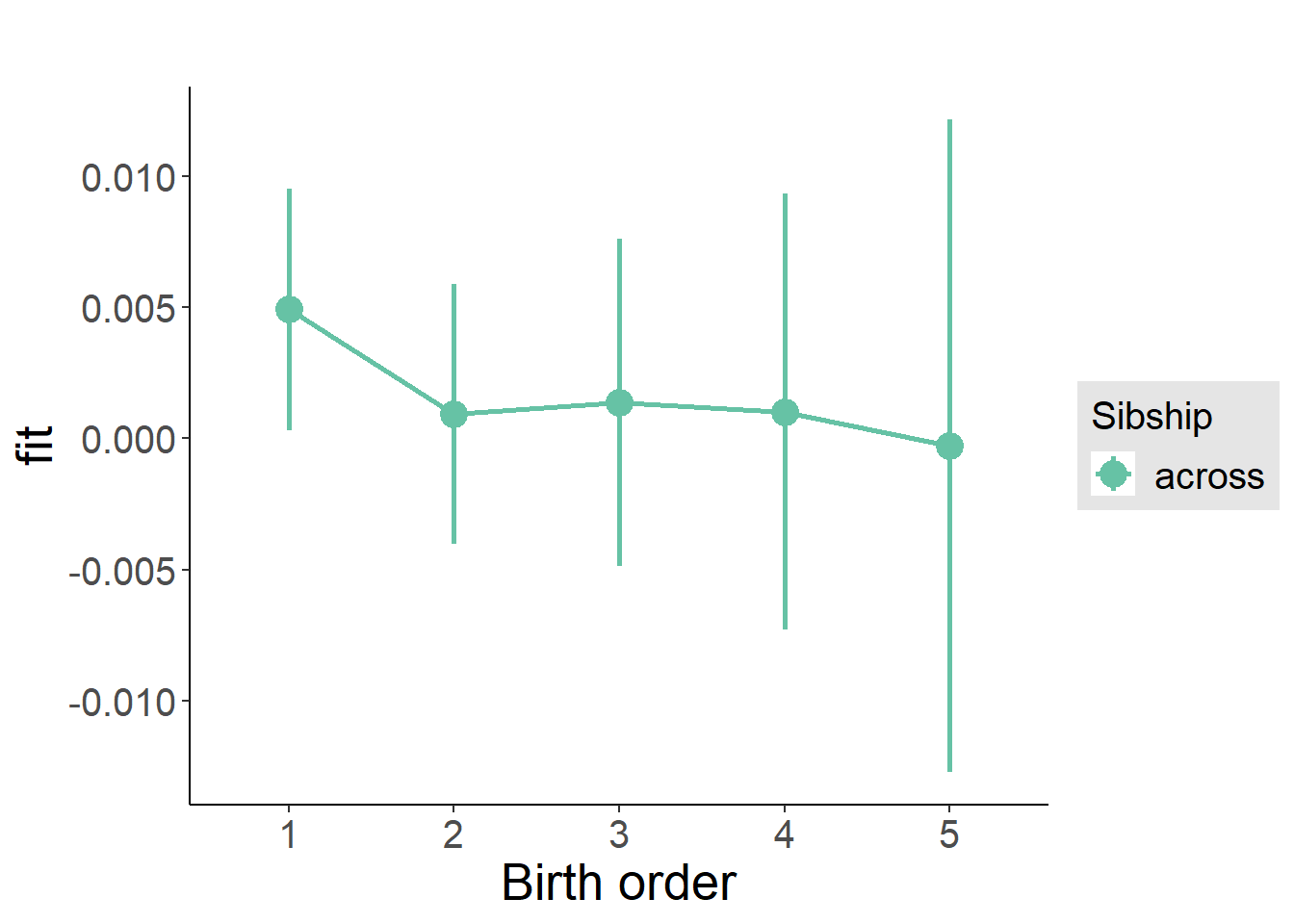
Add Interaction
Model Summary
m4_interaction = update(m3_birthorder_nonlinear, formula = . ~ . - birth_order_nonlinear - sibling_count + count_birth_order)## boundary (singular) fit: see ?isSingulartidy(m4_interaction, conf.int = T, conf.level = 0.995)| effect | group | term | estimate | std.error | statistic | df | p.value | conf.low | conf.high |
|---|---|---|---|---|---|---|---|---|---|
| fixed | NA | (Intercept) | -0.006905 | 0.0354 | -0.1951 | 2409 | 0.8453 | -0.1063 | 0.09245 |
| fixed | NA | poly(age, 3, raw = TRUE)1 | 0.0009308 | 0.003919 | 0.2375 | 2409 | 0.8123 | -0.01007 | 0.01193 |
| fixed | NA | poly(age, 3, raw = TRUE)2 | -0.00001523 | 0.0001388 | -0.1098 | 2409 | 0.9126 | -0.0004048 | 0.0003743 |
| fixed | NA | poly(age, 3, raw = TRUE)3 | -0.00000002515 | 0.000001574 | -0.01597 | 2409 | 0.9873 | -0.000004444 | 0.000004394 |
| fixed | NA | male | 0.001195 | 0.00168 | 0.7114 | 2409 | 0.4769 | -0.00352 | 0.00591 |
| fixed | NA | count_birth_order2/2 | -0.00646 | 0.003899 | -1.657 | 2409 | 0.09768 | -0.01741 | 0.004485 |
| fixed | NA | count_birth_order1/3 | -0.003133 | 0.003258 | -0.9616 | 2409 | 0.3364 | -0.01228 | 0.006012 |
| fixed | NA | count_birth_order2/3 | -0.006349 | 0.003546 | -1.79 | 2409 | 0.07351 | -0.0163 | 0.003605 |
| fixed | NA | count_birth_order3/3 | -0.006378 | 0.003934 | -1.621 | 2409 | 0.1051 | -0.01742 | 0.004664 |
| fixed | NA | count_birth_order1/4 | -0.006219 | 0.003546 | -1.754 | 2409 | 0.0796 | -0.01617 | 0.003735 |
| fixed | NA | count_birth_order2/4 | -0.006401 | 0.003733 | -1.715 | 2409 | 0.08649 | -0.01688 | 0.004076 |
| fixed | NA | count_birth_order3/4 | -0.006432 | 0.004041 | -1.592 | 2409 | 0.1115 | -0.01777 | 0.00491 |
| fixed | NA | count_birth_order4/4 | -0.00667 | 0.004384 | -1.521 | 2409 | 0.1283 | -0.01898 | 0.005636 |
| fixed | NA | count_birth_order1/5 | 0.001545 | 0.004294 | 0.3598 | 2409 | 0.719 | -0.01051 | 0.0136 |
| fixed | NA | count_birth_order2/5 | -0.006309 | 0.004397 | -1.435 | 2409 | 0.1514 | -0.01865 | 0.006033 |
| fixed | NA | count_birth_order3/5 | -0.006286 | 0.004522 | -1.39 | 2409 | 0.1646 | -0.01898 | 0.006408 |
| fixed | NA | count_birth_order4/5 | -0.006491 | 0.004595 | -1.413 | 2409 | 0.1579 | -0.01939 | 0.006407 |
| fixed | NA | count_birth_order5/5 | -0.006595 | 0.004667 | -1.413 | 2409 | 0.1578 | -0.01969 | 0.006505 |
| ran_pars | mother_pidlink | sd__(Intercept) | 0 | NA | NA | NA | NA | NA | NA |
| ran_pars | Residual | sd__Observation | 0.04061 | NA | NA | NA | NA | NA | NA |
Coefficient Plot
plot_birthorder(m4_interaction)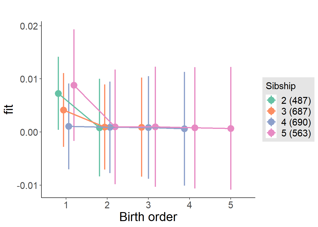
Model Comparison
###### Model 1 - Model 2
anova(m1_covariates_only, m2_birthorder_linear, m3_birthorder_nonlinear, m4_interaction)## refitting model(s) with ML (instead of REML)| Df | AIC | BIC | logLik | deviance | Chisq | Chi Df | Pr(>Chisq) |
|---|---|---|---|---|---|---|---|
| 10 | -8654 | -8596 | 4337 | -8674 | NA | NA | NA |
| 11 | -8655 | -8591 | 4338 | -8677 | 3.054 | 1 | 0.08056 |
| 14 | -8651 | -8570 | 4339 | -8679 | 1.967 | 3 | 0.5794 |
| 20 | -8641 | -8525 | 4341 | -8681 | 2.604 | 6 | 0.8567 |
Parental full sibling order
outcome_parental_m1 <- update(m2_birthorder_linear, data = birthorder %>%
mutate(sibling_count = sibling_count_genes_factor,
birth_order_nonlinear = birthorder_genes_factor,
birth_order = birthorder_genes,
count_birth_order = count_birthorder_genes
) %>%
filter(sibling_count != "1"))## boundary (singular) fit: see ?isSingularcompare_models_markdown(outcome_parental_m1)Basic Model
Model Summary
m1_covariates_only <- update(m2_birthorder_linear, formula = . ~ . - birth_order)## boundary (singular) fit: see ?isSingulartidy(m1_covariates_only, conf.int = T, conf.level = 0.995)| effect | group | term | estimate | std.error | statistic | df | p.value | conf.low | conf.high |
|---|---|---|---|---|---|---|---|---|---|
| fixed | NA | (Intercept) | -0.01083 | 0.0329 | -0.3293 | 2638 | 0.7419 | -0.1032 | 0.08151 |
| fixed | NA | poly(age, 3, raw = TRUE)1 | 0.001152 | 0.003651 | 0.3154 | 2638 | 0.7524 | -0.009096 | 0.0114 |
| fixed | NA | poly(age, 3, raw = TRUE)2 | -0.00002768 | 0.0001296 | -0.2136 | 2638 | 0.8309 | -0.0003915 | 0.0003361 |
| fixed | NA | poly(age, 3, raw = TRUE)3 | 0.0000001659 | 0.000001474 | 0.1126 | 2638 | 0.9104 | -0.000003971 | 0.000004303 |
| fixed | NA | male | 0.001165 | 0.001535 | 0.7592 | 2638 | 0.4478 | -0.003143 | 0.005474 |
| fixed | NA | sibling_count3 | -0.002126 | 0.002061 | -1.031 | 2638 | 0.3025 | -0.007912 | 0.00366 |
| fixed | NA | sibling_count4 | -0.003264 | 0.002155 | -1.515 | 2638 | 0.1299 | -0.009314 | 0.002785 |
| fixed | NA | sibling_count5 | -0.001038 | 0.002452 | -0.4232 | 2638 | 0.6722 | -0.007922 | 0.005846 |
| ran_pars | mother_pidlink | sd__(Intercept) | 0.0000000009743 | NA | NA | NA | NA | NA | NA |
| ran_pars | Residual | sd__Observation | 0.03888 | NA | NA | NA | NA | NA | NA |
Coefficient Plot
plot(allEffects(m1_covariates_only, confidence.level = 0.995))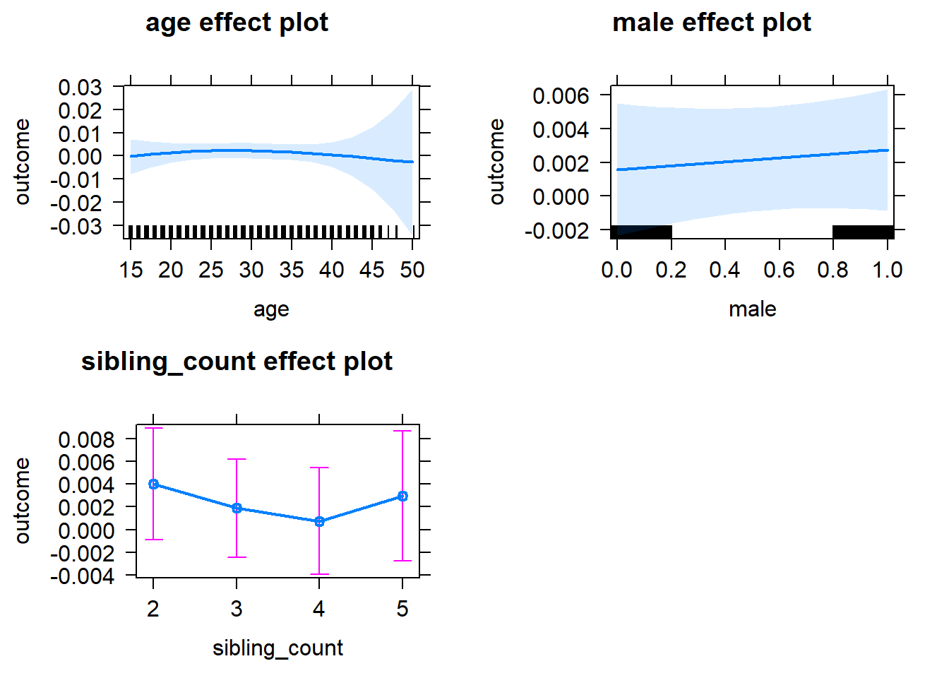
Add Birth Order Linear
Model Summary
tidy(m2_birthorder_linear, conf.int = T, conf.level = 0.995)| effect | group | term | estimate | std.error | statistic | df | p.value | conf.low | conf.high |
|---|---|---|---|---|---|---|---|---|---|
| fixed | NA | (Intercept) | -0.01045 | 0.03288 | -0.3178 | 2637 | 0.7507 | -0.1028 | 0.08185 |
| fixed | NA | birth_order | -0.001479 | 0.0007882 | -1.877 | 2637 | 0.06064 | -0.003692 | 0.0007332 |
| fixed | NA | poly(age, 3, raw = TRUE)1 | 0.001284 | 0.00365 | 0.3517 | 2637 | 0.7251 | -0.008961 | 0.01153 |
| fixed | NA | poly(age, 3, raw = TRUE)2 | -0.00002994 | 0.0001295 | -0.2311 | 2637 | 0.8172 | -0.0003936 | 0.0003337 |
| fixed | NA | poly(age, 3, raw = TRUE)3 | 0.0000001561 | 0.000001473 | 0.1059 | 2637 | 0.9156 | -0.000003979 | 0.000004291 |
| fixed | NA | male | 0.001144 | 0.001534 | 0.7458 | 2637 | 0.4559 | -0.003163 | 0.005451 |
| fixed | NA | sibling_count3 | -0.00142 | 0.002094 | -0.678 | 2637 | 0.4979 | -0.007299 | 0.004459 |
| fixed | NA | sibling_count4 | -0.001771 | 0.002296 | -0.7715 | 2637 | 0.4405 | -0.008217 | 0.004674 |
| fixed | NA | sibling_count5 | 0.001379 | 0.002769 | 0.498 | 2637 | 0.6186 | -0.006393 | 0.009151 |
| ran_pars | mother_pidlink | sd__(Intercept) | 0 | NA | NA | NA | NA | NA | NA |
| ran_pars | Residual | sd__Observation | 0.03886 | NA | NA | NA | NA | NA | NA |
Coefficient Plot
plot_birthorder2(m2_birthorder_linear, separate = FALSE)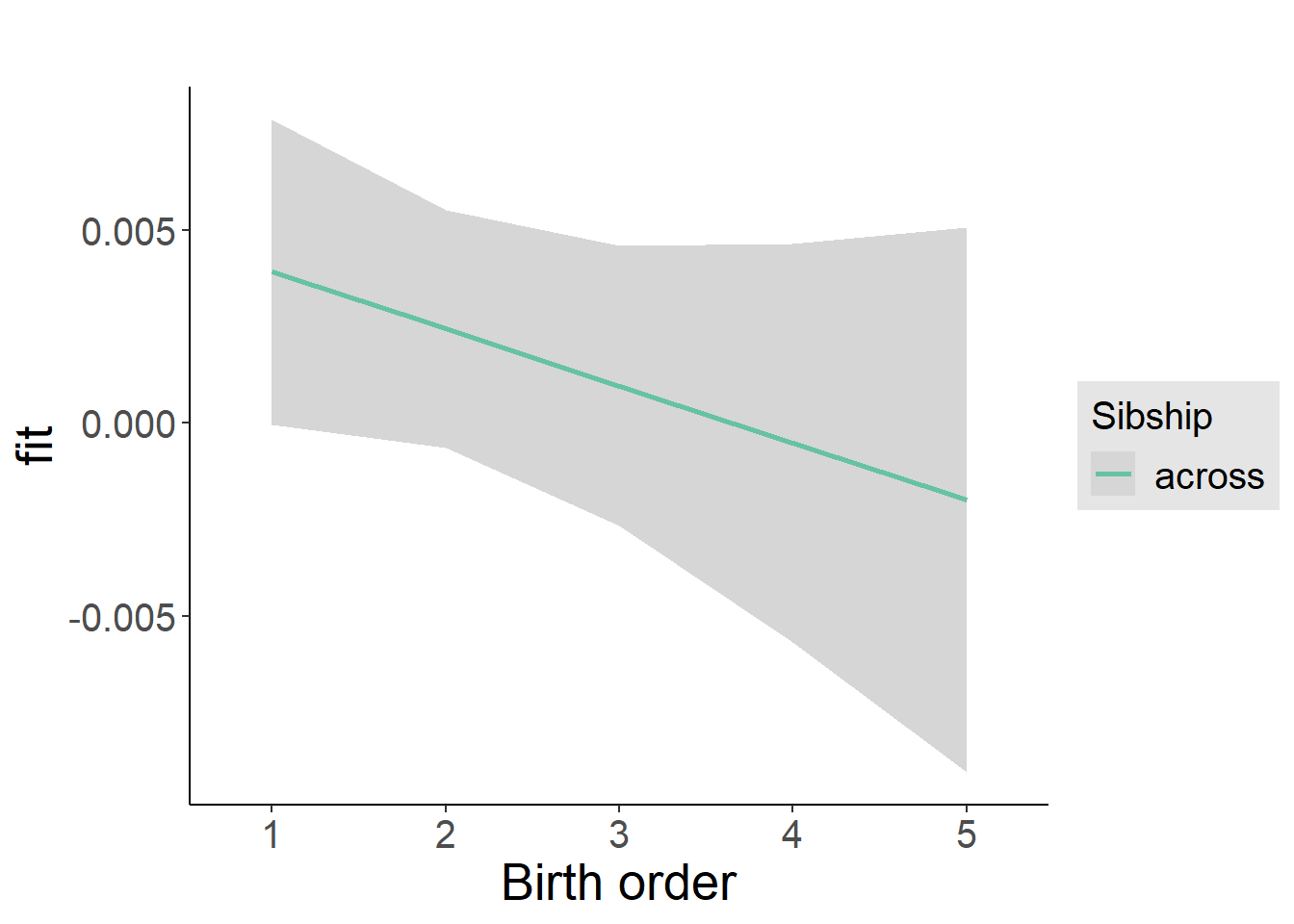
Add Birth Order Factor
Model Summary
m3_birthorder_nonlinear = update(m1_covariates_only, formula = . ~ . + birth_order_nonlinear)## boundary (singular) fit: see ?isSingulartidy(m3_birthorder_nonlinear, conf.int = T, conf.level = 0.995)| effect | group | term | estimate | std.error | statistic | df | p.value | conf.low | conf.high |
|---|---|---|---|---|---|---|---|---|---|
| fixed | NA | (Intercept) | -0.01096 | 0.03294 | -0.3326 | 2634 | 0.7394 | -0.1034 | 0.08151 |
| fixed | NA | poly(age, 3, raw = TRUE)1 | 0.001241 | 0.003655 | 0.3394 | 2634 | 0.7343 | -0.00902 | 0.0115 |
| fixed | NA | poly(age, 3, raw = TRUE)2 | -0.00002818 | 0.0001297 | -0.2172 | 2634 | 0.8281 | -0.0003924 | 0.000336 |
| fixed | NA | poly(age, 3, raw = TRUE)3 | 0.0000001361 | 0.000001475 | 0.09224 | 2634 | 0.9265 | -0.000004005 | 0.000004277 |
| fixed | NA | male | 0.001132 | 0.001536 | 0.737 | 2634 | 0.4612 | -0.003179 | 0.005442 |
| fixed | NA | sibling_count3 | -0.00141 | 0.002131 | -0.6616 | 2634 | 0.5083 | -0.00739 | 0.004571 |
| fixed | NA | sibling_count4 | -0.001969 | 0.00233 | -0.8451 | 2634 | 0.3981 | -0.00851 | 0.004572 |
| fixed | NA | sibling_count5 | 0.0009169 | 0.002818 | 0.3254 | 2634 | 0.7449 | -0.006992 | 0.008826 |
| fixed | NA | birth_order_nonlinear2 | -0.003533 | 0.001849 | -1.911 | 2634 | 0.05615 | -0.008723 | 0.001657 |
| fixed | NA | birth_order_nonlinear3 | -0.003265 | 0.002269 | -1.439 | 2634 | 0.1503 | -0.009635 | 0.003105 |
| fixed | NA | birth_order_nonlinear4 | -0.003861 | 0.003105 | -1.244 | 2634 | 0.2138 | -0.01258 | 0.004854 |
| fixed | NA | birth_order_nonlinear5 | -0.005587 | 0.004968 | -1.125 | 2634 | 0.2608 | -0.01953 | 0.008357 |
| ran_pars | mother_pidlink | sd__(Intercept) | 0.0000000008166 | NA | NA | NA | NA | NA | NA |
| ran_pars | Residual | sd__Observation | 0.03887 | NA | NA | NA | NA | NA | NA |
Coefficient Plot
plot_birthorder(m3_birthorder_nonlinear, separate = FALSE)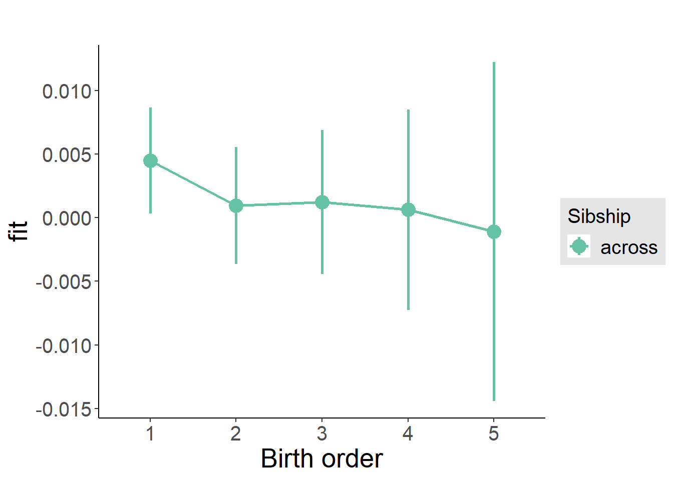
Add Interaction
Model Summary
m4_interaction = update(m3_birthorder_nonlinear, formula = . ~ . - birth_order_nonlinear - sibling_count + count_birth_order)## boundary (singular) fit: see ?isSingulartidy(m4_interaction, conf.int = T, conf.level = 0.995)| effect | group | term | estimate | std.error | statistic | df | p.value | conf.low | conf.high |
|---|---|---|---|---|---|---|---|---|---|
| fixed | NA | (Intercept) | -0.009204 | 0.03298 | -0.2791 | 2628 | 0.7802 | -0.1018 | 0.08337 |
| fixed | NA | poly(age, 3, raw = TRUE)1 | 0.00107 | 0.00366 | 0.2923 | 2628 | 0.77 | -0.009203 | 0.01134 |
| fixed | NA | poly(age, 3, raw = TRUE)2 | -0.00002089 | 0.0001299 | -0.1608 | 2628 | 0.8723 | -0.0003856 | 0.0003438 |
| fixed | NA | poly(age, 3, raw = TRUE)3 | 0.00000004016 | 0.000001478 | 0.02718 | 2628 | 0.9783 | -0.000004107 | 0.000004188 |
| fixed | NA | male | 0.001082 | 0.001538 | 0.7034 | 2628 | 0.4819 | -0.003235 | 0.005398 |
| fixed | NA | count_birth_order2/2 | -0.005017 | 0.003314 | -1.514 | 2628 | 0.1302 | -0.01432 | 0.004287 |
| fixed | NA | count_birth_order1/3 | -0.002348 | 0.002769 | -0.8478 | 2628 | 0.3966 | -0.01012 | 0.005426 |
| fixed | NA | count_birth_order2/3 | -0.004927 | 0.00308 | -1.6 | 2628 | 0.1098 | -0.01357 | 0.003719 |
| fixed | NA | count_birth_order3/3 | -0.005008 | 0.003321 | -1.508 | 2628 | 0.1316 | -0.01433 | 0.004313 |
| fixed | NA | count_birth_order1/4 | -0.004708 | 0.003258 | -1.445 | 2628 | 0.1486 | -0.01385 | 0.004438 |
| fixed | NA | count_birth_order2/4 | -0.00494 | 0.00342 | -1.444 | 2628 | 0.1488 | -0.01454 | 0.004661 |
| fixed | NA | count_birth_order3/4 | -0.004936 | 0.003551 | -1.39 | 2628 | 0.1646 | -0.0149 | 0.005031 |
| fixed | NA | count_birth_order4/4 | -0.005147 | 0.003853 | -1.336 | 2628 | 0.1817 | -0.01596 | 0.005668 |
| fixed | NA | count_birth_order1/5 | 0.004821 | 0.004272 | 1.129 | 2628 | 0.2592 | -0.00717 | 0.01681 |
| fixed | NA | count_birth_order2/5 | -0.00476 | 0.004762 | -0.9995 | 2628 | 0.3176 | -0.01813 | 0.008607 |
| fixed | NA | count_birth_order3/5 | -0.004904 | 0.004637 | -1.058 | 2628 | 0.2904 | -0.01792 | 0.008113 |
| fixed | NA | count_birth_order4/5 | -0.005181 | 0.004461 | -1.161 | 2628 | 0.2456 | -0.0177 | 0.007342 |
| fixed | NA | count_birth_order5/5 | -0.005186 | 0.004738 | -1.095 | 2628 | 0.2738 | -0.01849 | 0.008114 |
| ran_pars | mother_pidlink | sd__(Intercept) | 0 | NA | NA | NA | NA | NA | NA |
| ran_pars | Residual | sd__Observation | 0.03889 | NA | NA | NA | NA | NA | NA |
Coefficient Plot
plot_birthorder(m4_interaction)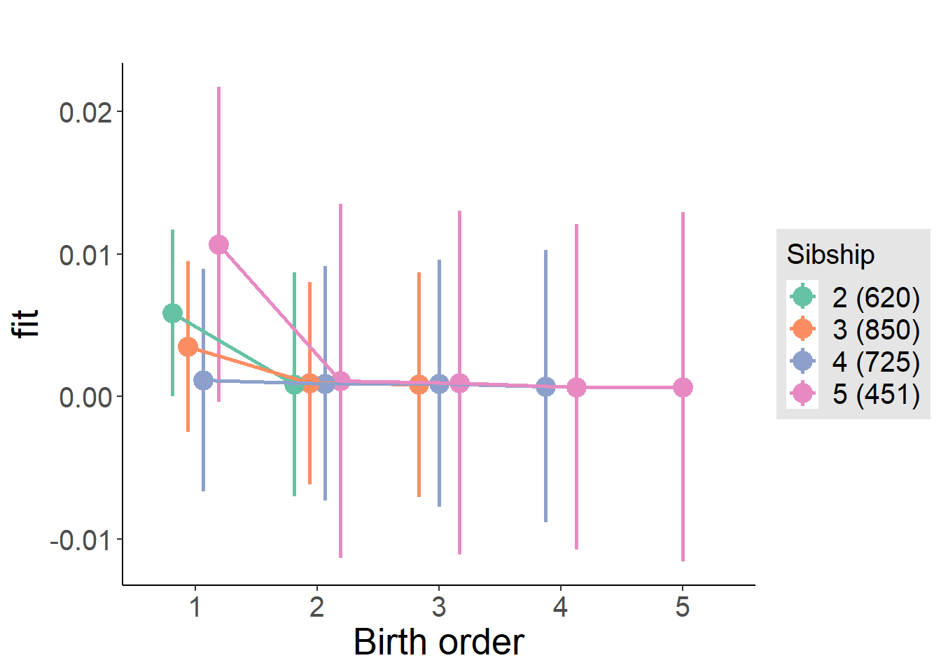
Model Comparison
###### Model 1 - Model 2
anova(m1_covariates_only, m2_birthorder_linear, m3_birthorder_nonlinear, m4_interaction)## refitting model(s) with ML (instead of REML)| Df | AIC | BIC | logLik | deviance | Chisq | Chi Df | Pr(>Chisq) |
|---|---|---|---|---|---|---|---|
| 10 | -9664 | -9605 | 4842 | -9684 | NA | NA | NA |
| 11 | -9665 | -9600 | 4844 | -9687 | 3.532 | 1 | 0.06018 |
| 14 | -9661 | -9578 | 4844 | -9689 | 1.543 | 3 | 0.6723 |
| 20 | -9652 | -9534 | 4846 | -9692 | 3.354 | 6 | 0.7633 |
Compare birth order specifications
library(coefplot)
multiplot(outcome_naive_m1, outcome_preg_m1, outcome_uterus_m1, outcome_parental_m1, dodgeHeight = 0.6,
intercept = FALSE)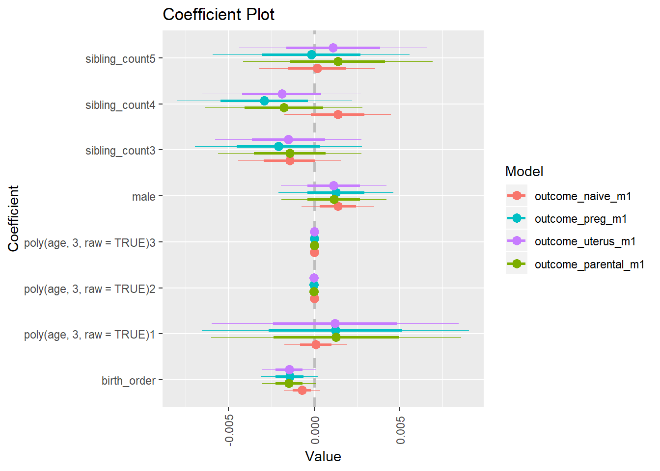
Sector_Electricity, gas, water
birthorder <- birthorder %>% mutate(outcome = `Sector_Electricity, gas, water`)
model = lmer(outcome ~ birth_order + poly(age, 3, raw = TRUE) + male + sibling_count + (1 | mother_pidlink),
data = birthorder)
compare_birthorder_specs(model)Naive birth order
outcome_naive_m1 <- update(m2_birthorder_linear, data = birthorder %>%
mutate(sibling_count = sibling_count_naive_factor,
birth_order_nonlinear = birthorder_naive_factor,
birth_order = birthorder_naive,
count_birth_order = count_birthorder_naive) %>%
filter(sibling_count != "1"))
compare_models_markdown(outcome_naive_m1)Basic Model
Model Summary
m1_covariates_only <- update(m2_birthorder_linear, formula = . ~ . - birth_order)
tidy(m1_covariates_only, conf.int = T, conf.level = 0.995)| effect | group | term | estimate | std.error | statistic | df | p.value | conf.low | conf.high |
|---|---|---|---|---|---|---|---|---|---|
| fixed | NA | (Intercept) | 0.007924 | 0.03945 | 0.2009 | 4200 | 0.8408 | -0.1028 | 0.1187 |
| fixed | NA | poly(age, 3, raw = TRUE)1 | 0.0003106 | 0.003504 | 0.08864 | 4058 | 0.9294 | -0.009525 | 0.01015 |
| fixed | NA | poly(age, 3, raw = TRUE)2 | 0.00001944 | 0.00009688 | 0.2007 | 3909 | 0.8409 | -0.0002525 | 0.0002914 |
| fixed | NA | poly(age, 3, raw = TRUE)3 | -0.0000003744 | 0.0000008437 | -0.4437 | 3783 | 0.6573 | -0.000002743 | 0.000001994 |
| fixed | NA | male | -0.000236 | 0.004065 | -0.05806 | 4627 | 0.9537 | -0.01165 | 0.01117 |
| fixed | NA | sibling_count3 | -0.006399 | 0.005721 | -1.119 | 3375 | 0.2634 | -0.02246 | 0.009659 |
| fixed | NA | sibling_count4 | 0.0007961 | 0.00577 | 0.138 | 3069 | 0.8903 | -0.0154 | 0.01699 |
| fixed | NA | sibling_count5 | -0.01126 | 0.005987 | -1.881 | 2792 | 0.06007 | -0.02807 | 0.005543 |
| ran_pars | mother_pidlink | sd__(Intercept) | 0.0251 | NA | NA | NA | NA | NA | NA |
| ran_pars | Residual | sd__Observation | 0.1348 | NA | NA | NA | NA | NA | NA |
Coefficient Plot
plot(allEffects(m1_covariates_only, confidence.level = 0.995))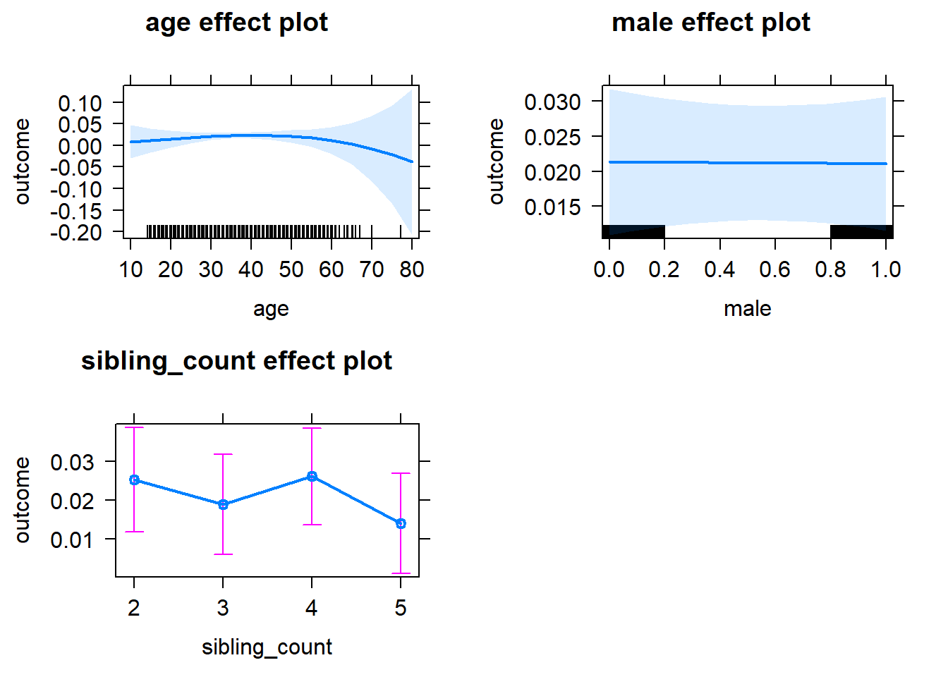
Add Birth Order Linear
Model Summary
tidy(m2_birthorder_linear, conf.int = T, conf.level = 0.995)| effect | group | term | estimate | std.error | statistic | df | p.value | conf.low | conf.high |
|---|---|---|---|---|---|---|---|---|---|
| fixed | NA | (Intercept) | 0.008121 | 0.03945 | 0.2058 | 4200 | 0.8369 | -0.1026 | 0.1189 |
| fixed | NA | birth_order | 0.0007092 | 0.002016 | 0.3517 | 4232 | 0.7251 | -0.004951 | 0.006369 |
| fixed | NA | poly(age, 3, raw = TRUE)1 | 0.0002023 | 0.003518 | 0.05751 | 4059 | 0.9541 | -0.009672 | 0.01008 |
| fixed | NA | poly(age, 3, raw = TRUE)2 | 0.00002213 | 0.00009719 | 0.2277 | 3902 | 0.8199 | -0.0002507 | 0.0002949 |
| fixed | NA | poly(age, 3, raw = TRUE)3 | -0.0000003925 | 0.0000008454 | -0.4643 | 3776 | 0.6425 | -0.000002766 | 0.000001981 |
| fixed | NA | male | -0.0002264 | 0.004066 | -0.0557 | 4626 | 0.9556 | -0.01164 | 0.01119 |
| fixed | NA | sibling_count3 | -0.006671 | 0.005773 | -1.156 | 3462 | 0.248 | -0.02288 | 0.009534 |
| fixed | NA | sibling_count4 | 0.0002128 | 0.006004 | 0.03544 | 3439 | 0.9717 | -0.01664 | 0.01707 |
| fixed | NA | sibling_count5 | -0.01218 | 0.006532 | -1.865 | 3533 | 0.06232 | -0.03052 | 0.006156 |
| ran_pars | mother_pidlink | sd__(Intercept) | 0.02511 | NA | NA | NA | NA | NA | NA |
| ran_pars | Residual | sd__Observation | 0.1348 | NA | NA | NA | NA | NA | NA |
Coefficient Plot
plot_birthorder2(m2_birthorder_linear, separate = FALSE)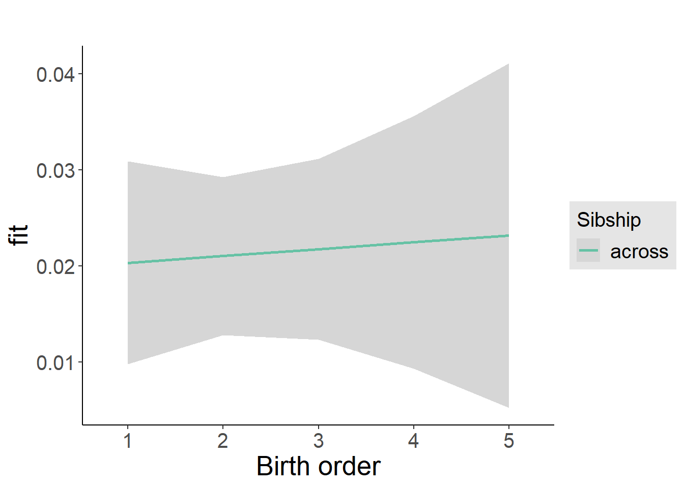
Add Birth Order Factor
Model Summary
m3_birthorder_nonlinear = update(m1_covariates_only, formula = . ~ . + birth_order_nonlinear)
tidy(m3_birthorder_nonlinear, conf.int = T, conf.level = 0.995)| effect | group | term | estimate | std.error | statistic | df | p.value | conf.low | conf.high |
|---|---|---|---|---|---|---|---|---|---|
| fixed | NA | (Intercept) | 0.007238 | 0.03958 | 0.1829 | 4206 | 0.8549 | -0.1039 | 0.1183 |
| fixed | NA | poly(age, 3, raw = TRUE)1 | 0.0001906 | 0.003519 | 0.05416 | 4055 | 0.9568 | -0.009686 | 0.01007 |
| fixed | NA | poly(age, 3, raw = TRUE)2 | 0.00002024 | 0.00009723 | 0.2082 | 3894 | 0.8351 | -0.0002527 | 0.0002932 |
| fixed | NA | poly(age, 3, raw = TRUE)3 | -0.0000003576 | 0.0000008461 | -0.4226 | 3762 | 0.6726 | -0.000002733 | 0.000002017 |
| fixed | NA | male | -0.0004508 | 0.004066 | -0.1109 | 4623 | 0.9117 | -0.01186 | 0.01096 |
| fixed | NA | sibling_count3 | -0.006238 | 0.005881 | -1.061 | 3618 | 0.2889 | -0.02275 | 0.01027 |
| fixed | NA | sibling_count4 | -0.0003201 | 0.006124 | -0.05228 | 3611 | 0.9583 | -0.01751 | 0.01687 |
| fixed | NA | sibling_count5 | -0.01017 | 0.006604 | -1.54 | 3632 | 0.1237 | -0.02871 | 0.00837 |
| fixed | NA | birth_order_nonlinear2 | 0.007765 | 0.004864 | 1.596 | 4103 | 0.1105 | -0.00589 | 0.02142 |
| fixed | NA | birth_order_nonlinear3 | 0.001531 | 0.006168 | 0.2482 | 4095 | 0.804 | -0.01578 | 0.01884 |
| fixed | NA | birth_order_nonlinear4 | 0.009456 | 0.008059 | 1.173 | 4086 | 0.2407 | -0.01317 | 0.03208 |
| fixed | NA | birth_order_nonlinear5 | -0.009664 | 0.01162 | -0.8314 | 4161 | 0.4058 | -0.0423 | 0.02297 |
| ran_pars | mother_pidlink | sd__(Intercept) | 0.02548 | NA | NA | NA | NA | NA | NA |
| ran_pars | Residual | sd__Observation | 0.1347 | NA | NA | NA | NA | NA | NA |
Coefficient Plot
plot_birthorder(m3_birthorder_nonlinear, separate = FALSE)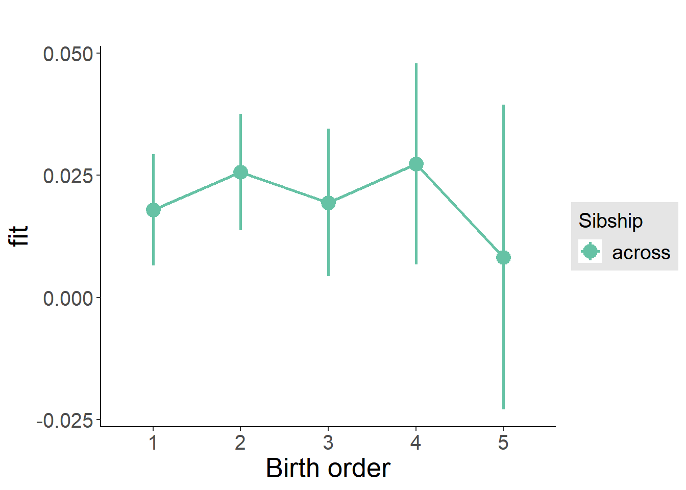
Add Interaction
Model Summary
m4_interaction = update(m3_birthorder_nonlinear, formula = . ~ . - birth_order_nonlinear - sibling_count + count_birth_order)
tidy(m4_interaction, conf.int = T, conf.level = 0.995)| effect | group | term | estimate | std.error | statistic | df | p.value | conf.low | conf.high |
|---|---|---|---|---|---|---|---|---|---|
| fixed | NA | (Intercept) | 0.004712 | 0.03964 | 0.1189 | 4211 | 0.9054 | -0.1066 | 0.116 |
| fixed | NA | poly(age, 3, raw = TRUE)1 | 0.0003728 | 0.003521 | 0.1059 | 4053 | 0.9157 | -0.009511 | 0.01026 |
| fixed | NA | poly(age, 3, raw = TRUE)2 | 0.00001582 | 0.00009726 | 0.1627 | 3891 | 0.8708 | -0.0002572 | 0.0002888 |
| fixed | NA | poly(age, 3, raw = TRUE)3 | -0.0000003263 | 0.0000008461 | -0.3856 | 3759 | 0.6998 | -0.000002701 | 0.000002049 |
| fixed | NA | male | -0.0005614 | 0.004067 | -0.1381 | 4616 | 0.8902 | -0.01198 | 0.01085 |
| fixed | NA | count_birth_order2/2 | 0.008889 | 0.008283 | 1.073 | 3992 | 0.2832 | -0.01436 | 0.03214 |
| fixed | NA | count_birth_order1/3 | -0.002423 | 0.007857 | -0.3085 | 4623 | 0.7578 | -0.02448 | 0.01963 |
| fixed | NA | count_birth_order2/3 | -0.003753 | 0.008748 | -0.429 | 4624 | 0.6679 | -0.02831 | 0.0208 |
| fixed | NA | count_birth_order3/3 | -0.003139 | 0.009626 | -0.3261 | 4624 | 0.7444 | -0.03016 | 0.02388 |
| fixed | NA | count_birth_order1/4 | -0.006796 | 0.008658 | -0.7849 | 4625 | 0.4325 | -0.0311 | 0.01751 |
| fixed | NA | count_birth_order2/4 | 0.02095 | 0.00929 | 2.255 | 4624 | 0.02419 | -0.005129 | 0.04702 |
| fixed | NA | count_birth_order3/4 | 0.001924 | 0.009805 | 0.1962 | 4624 | 0.8444 | -0.0256 | 0.02945 |
| fixed | NA | count_birth_order4/4 | 0.002518 | 0.01057 | 0.2381 | 4624 | 0.8118 | -0.02716 | 0.0322 |
| fixed | NA | count_birth_order1/5 | -0.005337 | 0.009769 | -0.5463 | 4625 | 0.5849 | -0.03276 | 0.02209 |
| fixed | NA | count_birth_order2/5 | -0.01199 | 0.01038 | -1.155 | 4625 | 0.248 | -0.04114 | 0.01715 |
| fixed | NA | count_birth_order3/5 | -0.01041 | 0.01092 | -0.9534 | 4625 | 0.3405 | -0.04108 | 0.02025 |
| fixed | NA | count_birth_order4/5 | 0.008429 | 0.01155 | 0.7301 | 4624 | 0.4653 | -0.02398 | 0.04084 |
| fixed | NA | count_birth_order5/5 | -0.01946 | 0.01157 | -1.682 | 4625 | 0.0926 | -0.05194 | 0.01302 |
| ran_pars | mother_pidlink | sd__(Intercept) | 0.02536 | NA | NA | NA | NA | NA | NA |
| ran_pars | Residual | sd__Observation | 0.1347 | NA | NA | NA | NA | NA | NA |
Coefficient Plot
plot_birthorder(m4_interaction)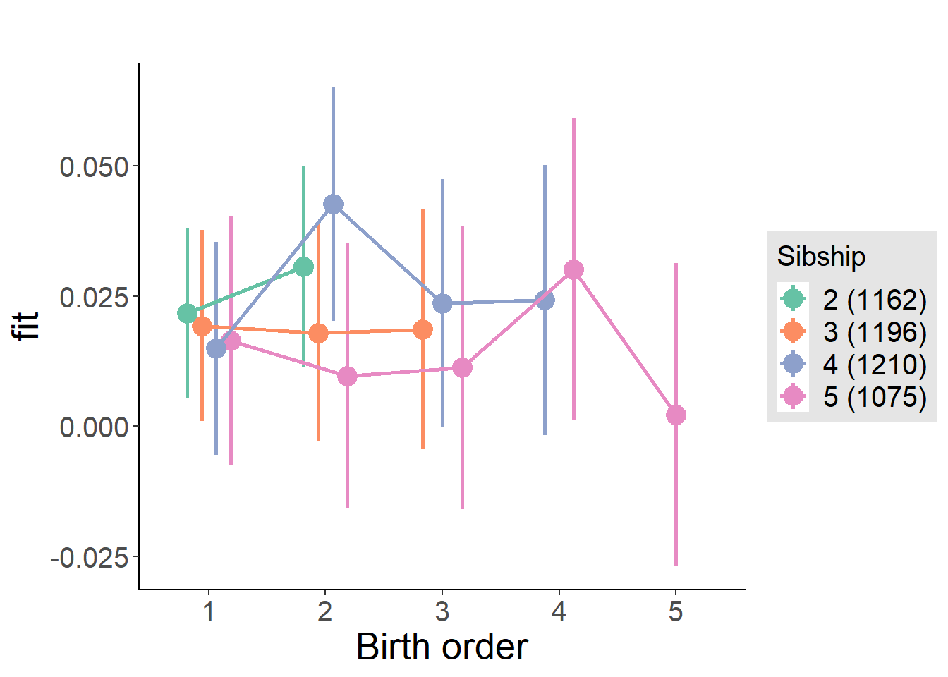
Model Comparison
###### Model 1 - Model 2
anova(m1_covariates_only, m2_birthorder_linear, m3_birthorder_nonlinear, m4_interaction)## refitting model(s) with ML (instead of REML)| Df | AIC | BIC | logLik | deviance | Chisq | Chi Df | Pr(>Chisq) |
|---|---|---|---|---|---|---|---|
| 10 | -5266 | -5201 | 2643 | -5286 | NA | NA | NA |
| 11 | -5264 | -5193 | 2643 | -5286 | 0.1235 | 1 | 0.7252 |
| 14 | -5263 | -5173 | 2645 | -5291 | 4.849 | 3 | 0.1832 |
| 20 | -5259 | -5130 | 2649 | -5299 | 7.929 | 6 | 0.2433 |
Maternal birth order
outcome_uterus_m1 <- update(m2_birthorder_linear, data = birthorder %>%
mutate(sibling_count = sibling_count_uterus_alive_factor,
birth_order_nonlinear = birthorder_uterus_alive_factor,
birth_order = birthorder_uterus_alive,
count_birth_order = count_birthorder_uterus_alive) %>%
filter(sibling_count != "1"))
compare_models_markdown(outcome_uterus_m1)Basic Model
Model Summary
m1_covariates_only <- update(m2_birthorder_linear, formula = . ~ . - birth_order)
tidy(m1_covariates_only, conf.int = T, conf.level = 0.995)| effect | group | term | estimate | std.error | statistic | df | p.value | conf.low | conf.high |
|---|---|---|---|---|---|---|---|---|---|
| fixed | NA | (Intercept) | -0.06505 | 0.1025 | -0.6344 | 2624 | 0.5259 | -0.3529 | 0.2228 |
| fixed | NA | poly(age, 3, raw = TRUE)1 | 0.008055 | 0.01135 | 0.7098 | 2623 | 0.4779 | -0.0238 | 0.03991 |
| fixed | NA | poly(age, 3, raw = TRUE)2 | -0.0002381 | 0.000402 | -0.5924 | 2622 | 0.5537 | -0.001366 | 0.0008902 |
| fixed | NA | poly(age, 3, raw = TRUE)3 | 0.000002178 | 0.00000456 | 0.4776 | 2620 | 0.633 | -0.00001062 | 0.00001498 |
| fixed | NA | male | -0.002941 | 0.004826 | -0.6092 | 2633 | 0.5424 | -0.01649 | 0.01061 |
| fixed | NA | sibling_count3 | -0.00462 | 0.006672 | -0.6924 | 2231 | 0.4887 | -0.02335 | 0.01411 |
| fixed | NA | sibling_count4 | 0.0006138 | 0.006895 | 0.08902 | 2065 | 0.9291 | -0.01874 | 0.01997 |
| fixed | NA | sibling_count5 | -0.003055 | 0.00767 | -0.3983 | 1816 | 0.6904 | -0.02458 | 0.01847 |
| ran_pars | mother_pidlink | sd__(Intercept) | 0.02553 | NA | NA | NA | NA | NA | NA |
| ran_pars | Residual | sd__Observation | 0.1195 | NA | NA | NA | NA | NA | NA |
Coefficient Plot
plot(allEffects(m1_covariates_only, confidence.level = 0.995))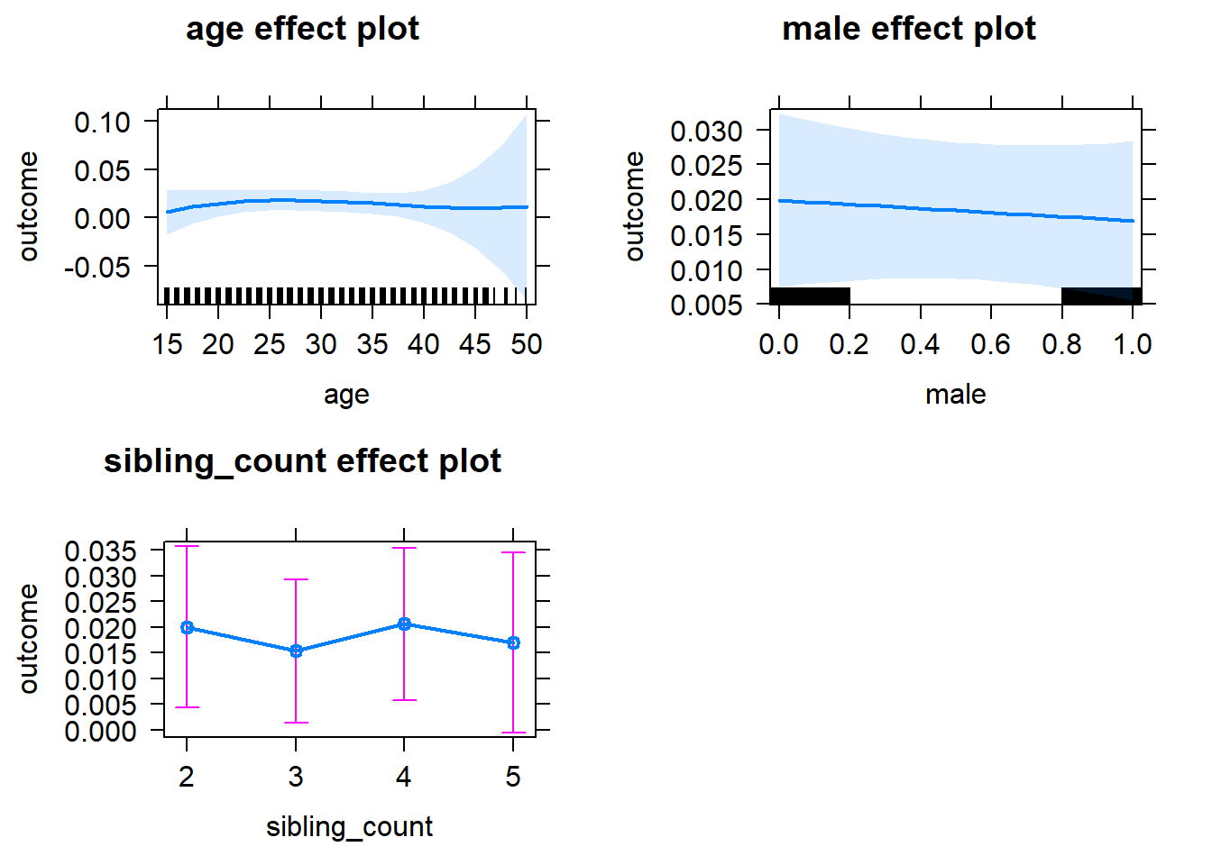
Add Birth Order Linear
Model Summary
tidy(m2_birthorder_linear, conf.int = T, conf.level = 0.995)| effect | group | term | estimate | std.error | statistic | df | p.value | conf.low | conf.high |
|---|---|---|---|---|---|---|---|---|---|
| fixed | NA | (Intercept) | -0.06472 | 0.1026 | -0.6311 | 2623 | 0.528 | -0.3526 | 0.2232 |
| fixed | NA | birth_order | -0.001559 | 0.002439 | -0.6389 | 2548 | 0.5229 | -0.008406 | 0.005289 |
| fixed | NA | poly(age, 3, raw = TRUE)1 | 0.008198 | 0.01135 | 0.7222 | 2622 | 0.4703 | -0.02367 | 0.04006 |
| fixed | NA | poly(age, 3, raw = TRUE)2 | -0.0002405 | 0.000402 | -0.5982 | 2621 | 0.5498 | -0.001369 | 0.000888 |
| fixed | NA | poly(age, 3, raw = TRUE)3 | 0.000002165 | 0.00000456 | 0.4748 | 2619 | 0.635 | -0.00001064 | 0.00001497 |
| fixed | NA | male | -0.002944 | 0.004827 | -0.6099 | 2632 | 0.542 | -0.01649 | 0.01061 |
| fixed | NA | sibling_count3 | -0.003886 | 0.006772 | -0.5738 | 2256 | 0.5662 | -0.02289 | 0.01512 |
| fixed | NA | sibling_count4 | 0.002203 | 0.007333 | 0.3004 | 2173 | 0.7639 | -0.01838 | 0.02279 |
| fixed | NA | sibling_count5 | -0.0004021 | 0.008726 | -0.04608 | 2108 | 0.9633 | -0.0249 | 0.02409 |
| ran_pars | mother_pidlink | sd__(Intercept) | 0.02568 | NA | NA | NA | NA | NA | NA |
| ran_pars | Residual | sd__Observation | 0.1195 | NA | NA | NA | NA | NA | NA |
Coefficient Plot
plot_birthorder2(m2_birthorder_linear, separate = FALSE)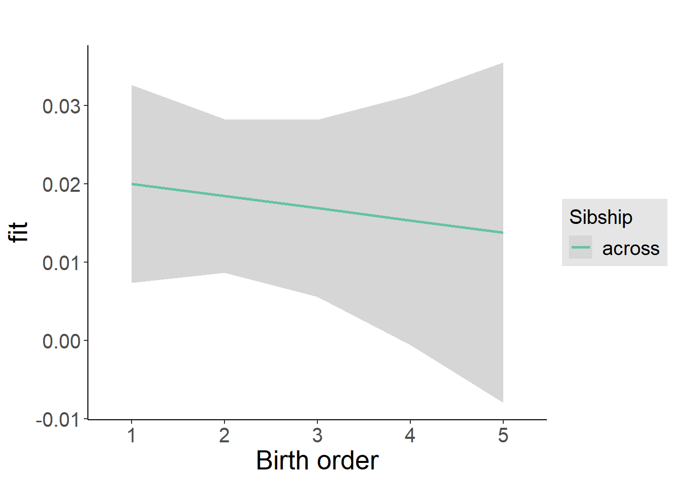
Add Birth Order Factor
Model Summary
m3_birthorder_nonlinear = update(m1_covariates_only, formula = . ~ . + birth_order_nonlinear)
tidy(m3_birthorder_nonlinear, conf.int = T, conf.level = 0.995)| effect | group | term | estimate | std.error | statistic | df | p.value | conf.low | conf.high |
|---|---|---|---|---|---|---|---|---|---|
| fixed | NA | (Intercept) | -0.06863 | 0.1028 | -0.6679 | 2619 | 0.5042 | -0.3571 | 0.2198 |
| fixed | NA | poly(age, 3, raw = TRUE)1 | 0.008229 | 0.01137 | 0.7239 | 2619 | 0.4692 | -0.02368 | 0.04014 |
| fixed | NA | poly(age, 3, raw = TRUE)2 | -0.0002427 | 0.0004026 | -0.6028 | 2618 | 0.5467 | -0.001373 | 0.0008875 |
| fixed | NA | poly(age, 3, raw = TRUE)3 | 0.000002196 | 0.000004566 | 0.4809 | 2617 | 0.6306 | -0.00001062 | 0.00001501 |
| fixed | NA | male | -0.002772 | 0.00483 | -0.5738 | 2629 | 0.5661 | -0.01633 | 0.01079 |
| fixed | NA | sibling_count3 | -0.003353 | 0.006877 | -0.4876 | 2302 | 0.6259 | -0.02266 | 0.01595 |
| fixed | NA | sibling_count4 | 0.004133 | 0.007436 | 0.5557 | 2219 | 0.5784 | -0.01674 | 0.02501 |
| fixed | NA | sibling_count5 | 0.00002649 | 0.00884 | 0.002997 | 2144 | 0.9976 | -0.02479 | 0.02484 |
| fixed | NA | birth_order_nonlinear2 | 0.005631 | 0.005837 | 0.9647 | 2392 | 0.3348 | -0.01075 | 0.02202 |
| fixed | NA | birth_order_nonlinear3 | -0.004838 | 0.007113 | -0.6802 | 2435 | 0.4965 | -0.0248 | 0.01513 |
| fixed | NA | birth_order_nonlinear4 | -0.01005 | 0.009466 | -1.062 | 2487 | 0.2885 | -0.03662 | 0.01652 |
| fixed | NA | birth_order_nonlinear5 | 0.005323 | 0.01467 | 0.3627 | 2450 | 0.7168 | -0.03587 | 0.04651 |
| ran_pars | mother_pidlink | sd__(Intercept) | 0.02606 | NA | NA | NA | NA | NA | NA |
| ran_pars | Residual | sd__Observation | 0.1194 | NA | NA | NA | NA | NA | NA |
Coefficient Plot
plot_birthorder(m3_birthorder_nonlinear, separate = FALSE)
Add Interaction
Model Summary
m4_interaction = update(m3_birthorder_nonlinear, formula = . ~ . - birth_order_nonlinear - sibling_count + count_birth_order)
tidy(m4_interaction, conf.int = T, conf.level = 0.995)| effect | group | term | estimate | std.error | statistic | df | p.value | conf.low | conf.high |
|---|---|---|---|---|---|---|---|---|---|
| fixed | NA | (Intercept) | -0.06998 | 0.1029 | -0.6802 | 2614 | 0.4965 | -0.3588 | 0.2188 |
| fixed | NA | poly(age, 3, raw = TRUE)1 | 0.00842 | 0.01138 | 0.7397 | 2613 | 0.4596 | -0.02353 | 0.04037 |
| fixed | NA | poly(age, 3, raw = TRUE)2 | -0.0002508 | 0.0004032 | -0.622 | 2612 | 0.534 | -0.001383 | 0.0008809 |
| fixed | NA | poly(age, 3, raw = TRUE)3 | 0.000002296 | 0.000004573 | 0.502 | 2611 | 0.6157 | -0.00001054 | 0.00001513 |
| fixed | NA | male | -0.002537 | 0.004839 | -0.5243 | 2623 | 0.6001 | -0.01612 | 0.01105 |
| fixed | NA | count_birth_order2/2 | 0.005499 | 0.01065 | 0.5166 | 2380 | 0.6055 | -0.02438 | 0.03538 |
| fixed | NA | count_birth_order1/3 | -0.004257 | 0.008863 | -0.4804 | 2624 | 0.631 | -0.02914 | 0.02062 |
| fixed | NA | count_birth_order2/3 | 0.00115 | 0.009852 | 0.1168 | 2624 | 0.907 | -0.0265 | 0.0288 |
| fixed | NA | count_birth_order3/3 | -0.005093 | 0.01074 | -0.4744 | 2623 | 0.6352 | -0.03523 | 0.02504 |
| fixed | NA | count_birth_order1/4 | 0.007385 | 0.0102 | 0.7242 | 2624 | 0.469 | -0.02124 | 0.03601 |
| fixed | NA | count_birth_order2/4 | 0.005426 | 0.0108 | 0.5026 | 2624 | 0.6153 | -0.02488 | 0.03573 |
| fixed | NA | count_birth_order3/4 | 0.001932 | 0.0112 | 0.1726 | 2622 | 0.863 | -0.0295 | 0.03336 |
| fixed | NA | count_birth_order4/4 | -0.008564 | 0.01197 | -0.7153 | 2623 | 0.4745 | -0.04217 | 0.02504 |
| fixed | NA | count_birth_order1/5 | -0.004143 | 0.01347 | -0.3077 | 2624 | 0.7583 | -0.04194 | 0.03365 |
| fixed | NA | count_birth_order2/5 | 0.01853 | 0.01449 | 1.279 | 2623 | 0.201 | -0.02214 | 0.05921 |
| fixed | NA | count_birth_order3/5 | -0.0153 | 0.01376 | -1.112 | 2622 | 0.2664 | -0.05393 | 0.02333 |
| fixed | NA | count_birth_order4/5 | -0.006532 | 0.01341 | -0.4869 | 2620 | 0.6263 | -0.04419 | 0.03112 |
| fixed | NA | count_birth_order5/5 | 0.005351 | 0.01411 | 0.3792 | 2619 | 0.7046 | -0.03426 | 0.04496 |
| ran_pars | mother_pidlink | sd__(Intercept) | 0.02613 | NA | NA | NA | NA | NA | NA |
| ran_pars | Residual | sd__Observation | 0.1195 | NA | NA | NA | NA | NA | NA |
Coefficient Plot
plot_birthorder(m4_interaction)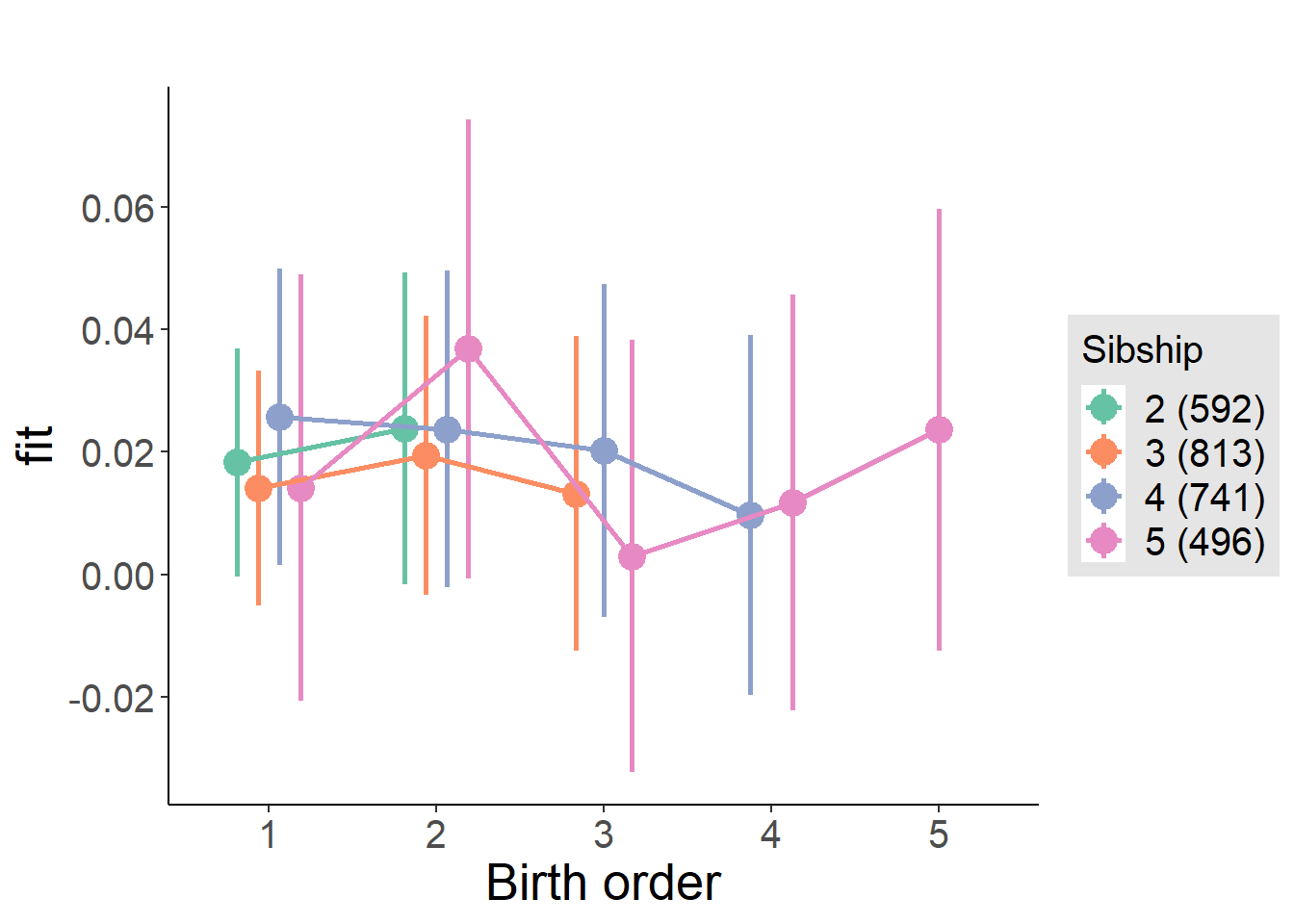
Model Comparison
###### Model 1 - Model 2
anova(m1_covariates_only, m2_birthorder_linear, m3_birthorder_nonlinear, m4_interaction)## refitting model(s) with ML (instead of REML)| Df | AIC | BIC | logLik | deviance | Chisq | Chi Df | Pr(>Chisq) |
|---|---|---|---|---|---|---|---|
| 10 | -3599 | -3540 | 1809 | -3619 | NA | NA | NA |
| 11 | -3597 | -3533 | 1810 | -3619 | 0.4076 | 1 | 0.5232 |
| 14 | -3595 | -3512 | 1811 | -3623 | 3.435 | 3 | 0.3292 |
| 20 | -3585 | -3468 | 1813 | -3625 | 2.7 | 6 | 0.8454 |
Maternal pregnancy order
outcome_preg_m1 <- update(m2_birthorder_linear, data = birthorder %>%
mutate(sibling_count = sibling_count_uterus_preg_factor,
birth_order_nonlinear = birthorder_uterus_preg_factor,
birth_order = birthorder_uterus_preg,
count_birth_order = count_birthorder_uterus_preg
) %>%
filter(sibling_count != "1"))
compare_models_markdown(outcome_preg_m1)Basic Model
Model Summary
m1_covariates_only <- update(m2_birthorder_linear, formula = . ~ . - birth_order)
tidy(m1_covariates_only, conf.int = T, conf.level = 0.995)| effect | group | term | estimate | std.error | statistic | df | p.value | conf.low | conf.high |
|---|---|---|---|---|---|---|---|---|---|
| fixed | NA | (Intercept) | -0.0684 | 0.1066 | -0.6415 | 2413 | 0.5212 | -0.3677 | 0.2309 |
| fixed | NA | poly(age, 3, raw = TRUE)1 | 0.008918 | 0.01181 | 0.7553 | 2413 | 0.4501 | -0.02422 | 0.04206 |
| fixed | NA | poly(age, 3, raw = TRUE)2 | -0.0002817 | 0.0004182 | -0.6735 | 2412 | 0.5007 | -0.001456 | 0.0008923 |
| fixed | NA | poly(age, 3, raw = TRUE)3 | 0.000002804 | 0.000004745 | 0.5909 | 2410 | 0.5546 | -0.00001052 | 0.00001612 |
| fixed | NA | male | -0.001801 | 0.005055 | -0.3564 | 2417 | 0.7216 | -0.01599 | 0.01239 |
| fixed | NA | sibling_count3 | -0.005572 | 0.007359 | -0.7571 | 2062 | 0.4491 | -0.02623 | 0.01509 |
| fixed | NA | sibling_count4 | -0.005431 | 0.007442 | -0.7298 | 1963 | 0.4656 | -0.02632 | 0.01546 |
| fixed | NA | sibling_count5 | -0.001223 | 0.007839 | -0.156 | 1818 | 0.8761 | -0.02323 | 0.02078 |
| ran_pars | mother_pidlink | sd__(Intercept) | 0.0282 | NA | NA | NA | NA | NA | NA |
| ran_pars | Residual | sd__Observation | 0.1194 | NA | NA | NA | NA | NA | NA |
Coefficient Plot
plot(allEffects(m1_covariates_only, confidence.level = 0.995))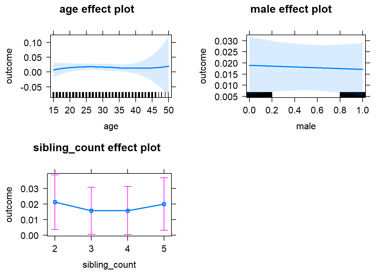
Add Birth Order Linear
Model Summary
tidy(m2_birthorder_linear, conf.int = T, conf.level = 0.995)| effect | group | term | estimate | std.error | statistic | df | p.value | conf.low | conf.high |
|---|---|---|---|---|---|---|---|---|---|
| fixed | NA | (Intercept) | -0.06819 | 0.1067 | -0.6394 | 2412 | 0.5226 | -0.3676 | 0.2312 |
| fixed | NA | birth_order | -0.0002783 | 0.002481 | -0.1122 | 2369 | 0.9107 | -0.007241 | 0.006685 |
| fixed | NA | poly(age, 3, raw = TRUE)1 | 0.008931 | 0.01181 | 0.7563 | 2411 | 0.4496 | -0.02422 | 0.04208 |
| fixed | NA | poly(age, 3, raw = TRUE)2 | -0.0002818 | 0.0004183 | -0.6736 | 2411 | 0.5006 | -0.001456 | 0.0008924 |
| fixed | NA | poly(age, 3, raw = TRUE)3 | 0.000002799 | 0.000004746 | 0.5897 | 2409 | 0.5554 | -0.00001052 | 0.00001612 |
| fixed | NA | male | -0.001809 | 0.005056 | -0.3578 | 2416 | 0.7205 | -0.016 | 0.01238 |
| fixed | NA | sibling_count3 | -0.00544 | 0.007455 | -0.7297 | 2076 | 0.4657 | -0.02637 | 0.01549 |
| fixed | NA | sibling_count4 | -0.005169 | 0.007802 | -0.6626 | 2028 | 0.5077 | -0.02707 | 0.01673 |
| fixed | NA | sibling_count5 | -0.0007793 | 0.008783 | -0.08872 | 2017 | 0.9293 | -0.02543 | 0.02387 |
| ran_pars | mother_pidlink | sd__(Intercept) | 0.02823 | NA | NA | NA | NA | NA | NA |
| ran_pars | Residual | sd__Observation | 0.1194 | NA | NA | NA | NA | NA | NA |
Coefficient Plot
plot_birthorder2(m2_birthorder_linear, separate = FALSE)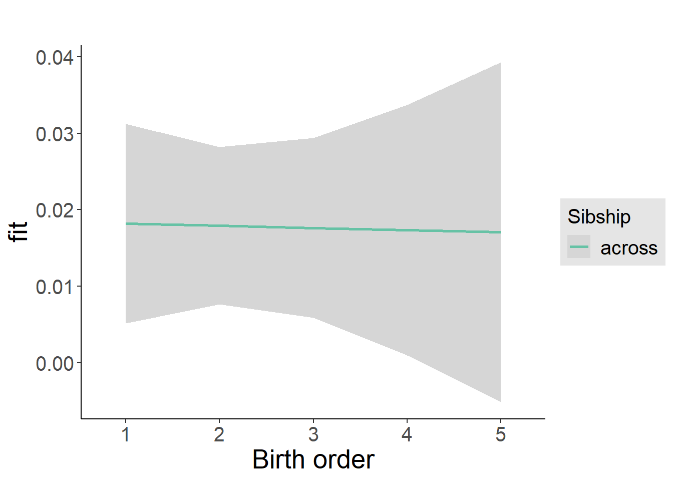
Add Birth Order Factor
Model Summary
m3_birthorder_nonlinear = update(m1_covariates_only, formula = . ~ . + birth_order_nonlinear)
tidy(m3_birthorder_nonlinear, conf.int = T, conf.level = 0.995)| effect | group | term | estimate | std.error | statistic | df | p.value | conf.low | conf.high |
|---|---|---|---|---|---|---|---|---|---|
| fixed | NA | (Intercept) | -0.07223 | 0.1068 | -0.6763 | 2408 | 0.4989 | -0.372 | 0.2276 |
| fixed | NA | poly(age, 3, raw = TRUE)1 | 0.008882 | 0.01182 | 0.7511 | 2408 | 0.4527 | -0.02431 | 0.04207 |
| fixed | NA | poly(age, 3, raw = TRUE)2 | -0.0002831 | 0.0004188 | -0.676 | 2407 | 0.4991 | -0.001459 | 0.0008925 |
| fixed | NA | poly(age, 3, raw = TRUE)3 | 0.000002837 | 0.000004751 | 0.5972 | 2406 | 0.5504 | -0.0000105 | 0.00001617 |
| fixed | NA | male | -0.001594 | 0.005054 | -0.3155 | 2413 | 0.7524 | -0.01578 | 0.01259 |
| fixed | NA | sibling_count3 | -0.004946 | 0.007559 | -0.6542 | 2111 | 0.513 | -0.02617 | 0.01627 |
| fixed | NA | sibling_count4 | -0.003435 | 0.007899 | -0.4349 | 2062 | 0.6637 | -0.02561 | 0.01874 |
| fixed | NA | sibling_count5 | 0.0009294 | 0.008838 | 0.1052 | 2035 | 0.9163 | -0.02388 | 0.02574 |
| fixed | NA | birth_order_nonlinear2 | 0.01469 | 0.006057 | 2.425 | 2185 | 0.01539 | -0.002313 | 0.03169 |
| fixed | NA | birth_order_nonlinear3 | -0.001744 | 0.007458 | -0.2338 | 2257 | 0.8152 | -0.02268 | 0.01919 |
| fixed | NA | birth_order_nonlinear4 | -0.004062 | 0.009839 | -0.4129 | 2307 | 0.6798 | -0.03168 | 0.02356 |
| fixed | NA | birth_order_nonlinear5 | 0.004612 | 0.01413 | 0.3264 | 2253 | 0.7442 | -0.03506 | 0.04428 |
| ran_pars | mother_pidlink | sd__(Intercept) | 0.02951 | NA | NA | NA | NA | NA | NA |
| ran_pars | Residual | sd__Observation | 0.119 | NA | NA | NA | NA | NA | NA |
Coefficient Plot
plot_birthorder(m3_birthorder_nonlinear, separate = FALSE)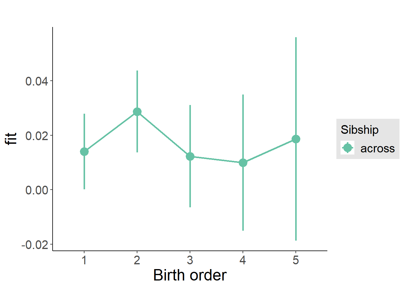
Add Interaction
Model Summary
m4_interaction = update(m3_birthorder_nonlinear, formula = . ~ . - birth_order_nonlinear - sibling_count + count_birth_order)
tidy(m4_interaction, conf.int = T, conf.level = 0.995)| effect | group | term | estimate | std.error | statistic | df | p.value | conf.low | conf.high |
|---|---|---|---|---|---|---|---|---|---|
| fixed | NA | (Intercept) | -0.06056 | 0.1069 | -0.5663 | 2402 | 0.5713 | -0.3608 | 0.2396 |
| fixed | NA | poly(age, 3, raw = TRUE)1 | 0.007735 | 0.01184 | 0.6532 | 2402 | 0.5137 | -0.0255 | 0.04097 |
| fixed | NA | poly(age, 3, raw = TRUE)2 | -0.0002404 | 0.0004194 | -0.5731 | 2401 | 0.5666 | -0.001418 | 0.0009369 |
| fixed | NA | poly(age, 3, raw = TRUE)3 | 0.000002332 | 0.000004758 | 0.4902 | 2400 | 0.624 | -0.00001102 | 0.00001569 |
| fixed | NA | male | -0.001669 | 0.005065 | -0.3296 | 2407 | 0.7417 | -0.01589 | 0.01255 |
| fixed | NA | count_birth_order2/2 | 0.009072 | 0.01167 | 0.7773 | 2210 | 0.437 | -0.02369 | 0.04183 |
| fixed | NA | count_birth_order1/3 | -0.0123 | 0.009829 | -1.252 | 2408 | 0.2108 | -0.03989 | 0.01529 |
| fixed | NA | count_birth_order2/3 | 0.01163 | 0.0107 | 1.087 | 2409 | 0.277 | -0.0184 | 0.04165 |
| fixed | NA | count_birth_order3/3 | -0.003251 | 0.01186 | -0.2742 | 2407 | 0.784 | -0.03654 | 0.03004 |
| fixed | NA | count_birth_order1/4 | -0.01014 | 0.0107 | -0.9474 | 2409 | 0.3435 | -0.04017 | 0.0199 |
| fixed | NA | count_birth_order2/4 | 0.0107 | 0.01126 | 0.9503 | 2409 | 0.342 | -0.0209 | 0.0423 |
| fixed | NA | count_birth_order3/4 | -0.002765 | 0.01218 | -0.227 | 2407 | 0.8204 | -0.03696 | 0.03143 |
| fixed | NA | count_birth_order4/4 | -0.007614 | 0.01322 | -0.5761 | 2406 | 0.5646 | -0.04471 | 0.02948 |
| fixed | NA | count_birth_order1/5 | 0.01608 | 0.01296 | 1.241 | 2409 | 0.2146 | -0.02029 | 0.05245 |
| fixed | NA | count_birth_order2/5 | 0.009684 | 0.01326 | 0.7302 | 2408 | 0.4653 | -0.02754 | 0.04691 |
| fixed | NA | count_birth_order3/5 | -0.01653 | 0.01363 | -1.212 | 2405 | 0.2255 | -0.05479 | 0.02174 |
| fixed | NA | count_birth_order4/5 | -0.00712 | 0.01385 | -0.5141 | 2404 | 0.6073 | -0.046 | 0.03176 |
| fixed | NA | count_birth_order5/5 | 0.003503 | 0.01406 | 0.2491 | 2401 | 0.8033 | -0.03597 | 0.04298 |
| ran_pars | mother_pidlink | sd__(Intercept) | 0.03001 | NA | NA | NA | NA | NA | NA |
| ran_pars | Residual | sd__Observation | 0.1188 | NA | NA | NA | NA | NA | NA |
Coefficient Plot
plot_birthorder(m4_interaction)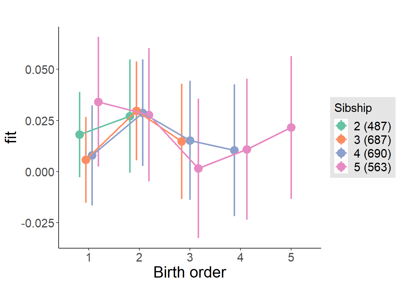
Model Comparison
###### Model 1 - Model 2
anova(m1_covariates_only, m2_birthorder_linear, m3_birthorder_nonlinear, m4_interaction)## refitting model(s) with ML (instead of REML)| Df | AIC | BIC | logLik | deviance | Chisq | Chi Df | Pr(>Chisq) |
|---|---|---|---|---|---|---|---|
| 10 | -3288 | -3230 | 1654 | -3308 | NA | NA | NA |
| 11 | -3286 | -3222 | 1654 | -3308 | 0.01217 | 1 | 0.9121 |
| 14 | -3288 | -3207 | 1658 | -3316 | 8.215 | 3 | 0.04177 |
| 20 | -3282 | -3166 | 1661 | -3322 | 6.093 | 6 | 0.4128 |
Parental full sibling order
outcome_parental_m1 <- update(m2_birthorder_linear, data = birthorder %>%
mutate(sibling_count = sibling_count_genes_factor,
birth_order_nonlinear = birthorder_genes_factor,
birth_order = birthorder_genes,
count_birth_order = count_birthorder_genes
) %>%
filter(sibling_count != "1"))
compare_models_markdown(outcome_parental_m1)Basic Model
Model Summary
m1_covariates_only <- update(m2_birthorder_linear, formula = . ~ . - birth_order)
tidy(m1_covariates_only, conf.int = T, conf.level = 0.995)| effect | group | term | estimate | std.error | statistic | df | p.value | conf.low | conf.high |
|---|---|---|---|---|---|---|---|---|---|
| fixed | NA | (Intercept) | -0.01603 | 0.1034 | -0.155 | 2626 | 0.8768 | -0.3063 | 0.2743 |
| fixed | NA | poly(age, 3, raw = TRUE)1 | 0.002543 | 0.01148 | 0.2216 | 2625 | 0.8246 | -0.02968 | 0.03476 |
| fixed | NA | poly(age, 3, raw = TRUE)2 | -0.00004377 | 0.0004075 | -0.1074 | 2624 | 0.9145 | -0.001188 | 0.0011 |
| fixed | NA | poly(age, 3, raw = TRUE)3 | 0.00000001926 | 0.000004635 | 0.004155 | 2622 | 0.9967 | -0.00001299 | 0.00001303 |
| fixed | NA | male | -0.004404 | 0.004819 | -0.9138 | 2637 | 0.3609 | -0.01793 | 0.009124 |
| fixed | NA | sibling_count3 | -0.005568 | 0.006519 | -0.8542 | 2266 | 0.3931 | -0.02387 | 0.01273 |
| fixed | NA | sibling_count4 | 0.002938 | 0.006828 | 0.4302 | 2110 | 0.6671 | -0.01623 | 0.0221 |
| fixed | NA | sibling_count5 | -0.001104 | 0.007798 | -0.1415 | 1787 | 0.8875 | -0.02299 | 0.02079 |
| ran_pars | mother_pidlink | sd__(Intercept) | 0.02368 | NA | NA | NA | NA | NA | NA |
| ran_pars | Residual | sd__Observation | 0.1198 | NA | NA | NA | NA | NA | NA |
Coefficient Plot
plot(allEffects(m1_covariates_only, confidence.level = 0.995))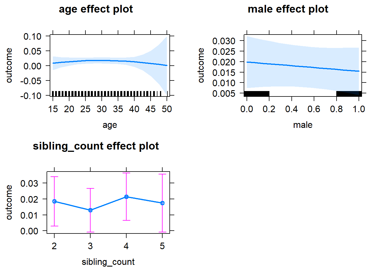
Add Birth Order Linear
Model Summary
tidy(m2_birthorder_linear, conf.int = T, conf.level = 0.995)| effect | group | term | estimate | std.error | statistic | df | p.value | conf.low | conf.high |
|---|---|---|---|---|---|---|---|---|---|
| fixed | NA | (Intercept) | -0.01566 | 0.1034 | -0.1514 | 2625 | 0.8797 | -0.306 | 0.2747 |
| fixed | NA | birth_order | -0.001587 | 0.002468 | -0.6431 | 2554 | 0.5202 | -0.008516 | 0.005342 |
| fixed | NA | poly(age, 3, raw = TRUE)1 | 0.002691 | 0.01148 | 0.2344 | 2624 | 0.8147 | -0.02954 | 0.03492 |
| fixed | NA | poly(age, 3, raw = TRUE)2 | -0.0000464 | 0.0004076 | -0.1139 | 2622 | 0.9094 | -0.00119 | 0.001098 |
| fixed | NA | poly(age, 3, raw = TRUE)3 | 0.00000001012 | 0.000004635 | 0.002184 | 2621 | 0.9983 | -0.000013 | 0.00001302 |
| fixed | NA | male | -0.004425 | 0.00482 | -0.9182 | 2636 | 0.3586 | -0.01795 | 0.009104 |
| fixed | NA | sibling_count3 | -0.00481 | 0.006626 | -0.7259 | 2289 | 0.468 | -0.02341 | 0.01379 |
| fixed | NA | sibling_count4 | 0.004543 | 0.007271 | 0.6248 | 2219 | 0.5322 | -0.01587 | 0.02495 |
| fixed | NA | sibling_count5 | 0.001493 | 0.008785 | 0.17 | 2055 | 0.865 | -0.02317 | 0.02615 |
| ran_pars | mother_pidlink | sd__(Intercept) | 0.02381 | NA | NA | NA | NA | NA | NA |
| ran_pars | Residual | sd__Observation | 0.1198 | NA | NA | NA | NA | NA | NA |
Coefficient Plot
plot_birthorder2(m2_birthorder_linear, separate = FALSE)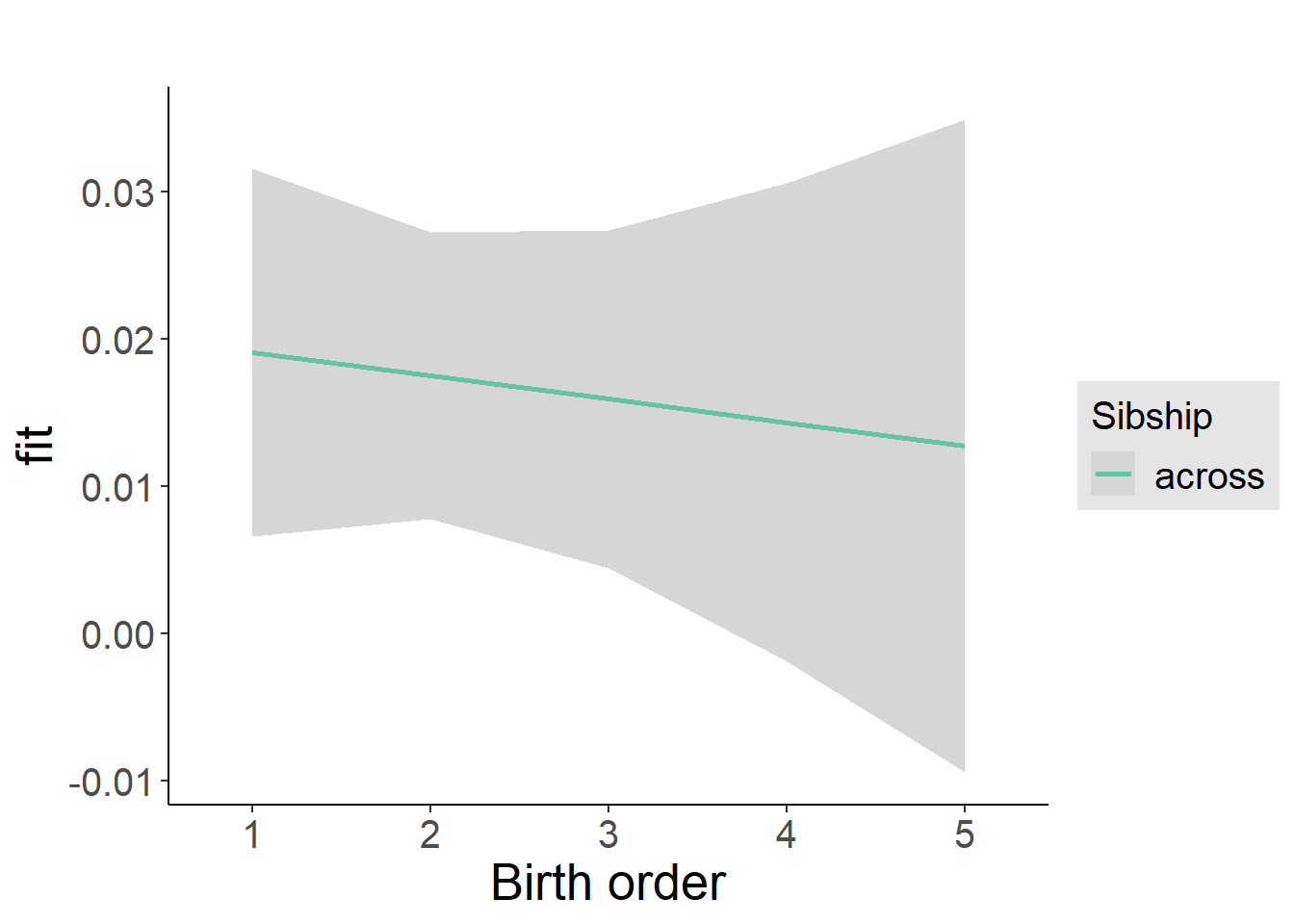
Add Birth Order Factor
Model Summary
m3_birthorder_nonlinear = update(m1_covariates_only, formula = . ~ . + birth_order_nonlinear)
tidy(m3_birthorder_nonlinear, conf.int = T, conf.level = 0.995)| effect | group | term | estimate | std.error | statistic | df | p.value | conf.low | conf.high |
|---|---|---|---|---|---|---|---|---|---|
| fixed | NA | (Intercept) | -0.01826 | 0.1036 | -0.1763 | 2621 | 0.8601 | -0.3091 | 0.2725 |
| fixed | NA | poly(age, 3, raw = TRUE)1 | 0.002578 | 0.0115 | 0.2243 | 2621 | 0.8226 | -0.02969 | 0.03485 |
| fixed | NA | poly(age, 3, raw = TRUE)2 | -0.00004309 | 0.0004081 | -0.1056 | 2619 | 0.9159 | -0.001189 | 0.001102 |
| fixed | NA | poly(age, 3, raw = TRUE)3 | -0.00000002531 | 0.00000464 | -0.005454 | 2618 | 0.9956 | -0.00001305 | 0.000013 |
| fixed | NA | male | -0.004399 | 0.004822 | -0.9122 | 2634 | 0.3617 | -0.01793 | 0.009137 |
| fixed | NA | sibling_count3 | -0.004139 | 0.006735 | -0.6145 | 2334 | 0.539 | -0.02304 | 0.01477 |
| fixed | NA | sibling_count4 | 0.006655 | 0.007373 | 0.9026 | 2261 | 0.3669 | -0.01404 | 0.02735 |
| fixed | NA | sibling_count5 | 0.001748 | 0.008933 | 0.1956 | 2099 | 0.8449 | -0.02333 | 0.02682 |
| fixed | NA | birth_order_nonlinear2 | 0.005275 | 0.005774 | 0.9135 | 2414 | 0.3611 | -0.01093 | 0.02148 |
| fixed | NA | birth_order_nonlinear3 | -0.005142 | 0.007092 | -0.725 | 2458 | 0.4685 | -0.02505 | 0.01476 |
| fixed | NA | birth_order_nonlinear4 | -0.0109 | 0.009711 | -1.123 | 2503 | 0.2616 | -0.03816 | 0.01636 |
| fixed | NA | birth_order_nonlinear5 | 0.007513 | 0.01553 | 0.4837 | 2483 | 0.6287 | -0.03609 | 0.05111 |
| ran_pars | mother_pidlink | sd__(Intercept) | 0.02398 | NA | NA | NA | NA | NA | NA |
| ran_pars | Residual | sd__Observation | 0.1197 | NA | NA | NA | NA | NA | NA |
Coefficient Plot
plot_birthorder(m3_birthorder_nonlinear, separate = FALSE)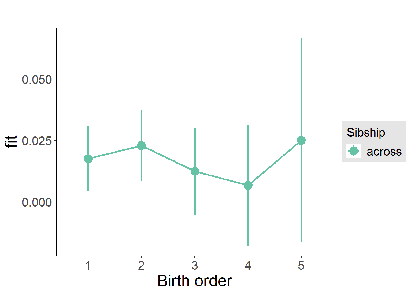
Add Interaction
Model Summary
m4_interaction = update(m3_birthorder_nonlinear, formula = . ~ . - birth_order_nonlinear - sibling_count + count_birth_order)
tidy(m4_interaction, conf.int = T, conf.level = 0.995)| effect | group | term | estimate | std.error | statistic | df | p.value | conf.low | conf.high |
|---|---|---|---|---|---|---|---|---|---|
| fixed | NA | (Intercept) | -0.01895 | 0.1037 | -0.1827 | 2615 | 0.855 | -0.3101 | 0.2722 |
| fixed | NA | poly(age, 3, raw = TRUE)1 | 0.002754 | 0.01151 | 0.2393 | 2615 | 0.8109 | -0.02955 | 0.03506 |
| fixed | NA | poly(age, 3, raw = TRUE)2 | -0.00005161 | 0.0004086 | -0.1263 | 2613 | 0.8995 | -0.001199 | 0.001095 |
| fixed | NA | poly(age, 3, raw = TRUE)3 | 0.00000008738 | 0.000004648 | 0.0188 | 2612 | 0.985 | -0.00001296 | 0.00001313 |
| fixed | NA | male | -0.004255 | 0.004829 | -0.8812 | 2628 | 0.3783 | -0.01781 | 0.0093 |
| fixed | NA | count_birth_order2/2 | 0.004488 | 0.01035 | 0.4336 | 2403 | 0.6646 | -0.02457 | 0.03354 |
| fixed | NA | count_birth_order1/3 | -0.004156 | 0.008698 | -0.4778 | 2628 | 0.6328 | -0.02857 | 0.02026 |
| fixed | NA | count_birth_order2/3 | -0.002799 | 0.009673 | -0.2894 | 2628 | 0.7723 | -0.02995 | 0.02435 |
| fixed | NA | count_birth_order3/3 | -0.00523 | 0.01042 | -0.5017 | 2626 | 0.6159 | -0.03449 | 0.02403 |
| fixed | NA | count_birth_order1/4 | 0.008228 | 0.01023 | 0.8039 | 2628 | 0.4215 | -0.0205 | 0.03695 |
| fixed | NA | count_birth_order2/4 | 0.0111 | 0.01074 | 1.034 | 2628 | 0.3013 | -0.01904 | 0.04125 |
| fixed | NA | count_birth_order3/4 | 0.002136 | 0.01115 | 0.1916 | 2627 | 0.848 | -0.02915 | 0.03343 |
| fixed | NA | count_birth_order4/4 | -0.007515 | 0.0121 | -0.6212 | 2627 | 0.5345 | -0.04147 | 0.02644 |
| fixed | NA | count_birth_order1/5 | -0.003897 | 0.01342 | -0.2904 | 2628 | 0.7715 | -0.04157 | 0.03377 |
| fixed | NA | count_birth_order2/5 | 0.02158 | 0.01495 | 1.443 | 2627 | 0.1491 | -0.02039 | 0.06355 |
| fixed | NA | count_birth_order3/5 | -0.01539 | 0.01456 | -1.057 | 2626 | 0.2907 | -0.05626 | 0.02548 |
| fixed | NA | count_birth_order4/5 | -0.004958 | 0.014 | -0.354 | 2625 | 0.7234 | -0.04427 | 0.03435 |
| fixed | NA | count_birth_order5/5 | 0.00907 | 0.01487 | 0.6098 | 2624 | 0.542 | -0.03268 | 0.05082 |
| ran_pars | mother_pidlink | sd__(Intercept) | 0.02393 | NA | NA | NA | NA | NA | NA |
| ran_pars | Residual | sd__Observation | 0.1198 | NA | NA | NA | NA | NA | NA |
Coefficient Plot
plot_birthorder(m4_interaction)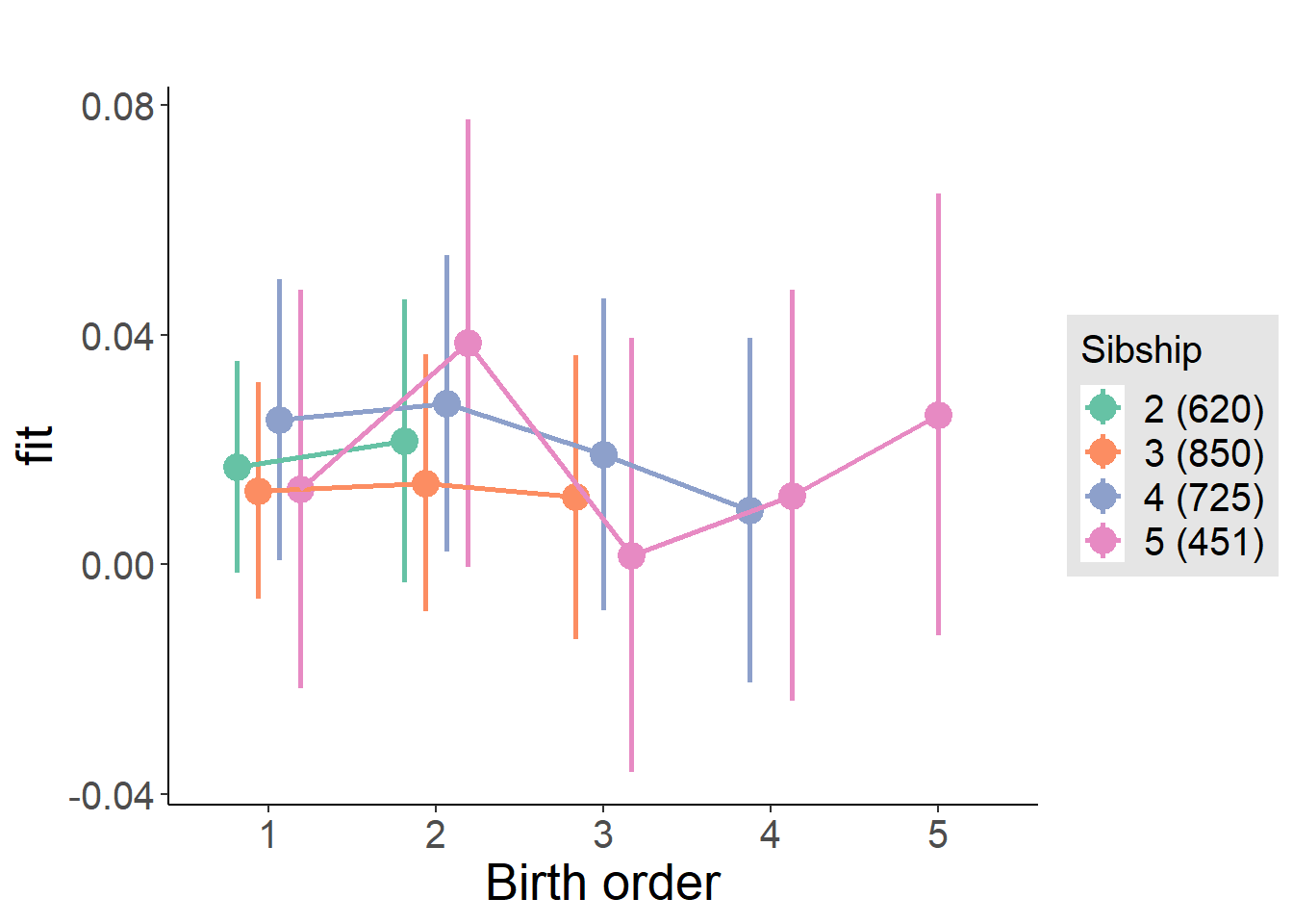
Model Comparison
###### Model 1 - Model 2
anova(m1_covariates_only, m2_birthorder_linear, m3_birthorder_nonlinear, m4_interaction)## refitting model(s) with ML (instead of REML)| Df | AIC | BIC | logLik | deviance | Chisq | Chi Df | Pr(>Chisq) |
|---|---|---|---|---|---|---|---|
| 10 | -3609 | -3550 | 1815 | -3629 | NA | NA | NA |
| 11 | -3607 | -3543 | 1815 | -3629 | 0.4132 | 1 | 0.5204 |
| 14 | -3605 | -3523 | 1817 | -3633 | 3.637 | 3 | 0.3035 |
| 20 | -3596 | -3479 | 1818 | -3636 | 3.027 | 6 | 0.8055 |
Compare birth order specifications
library(coefplot)
multiplot(outcome_naive_m1, outcome_preg_m1, outcome_uterus_m1, outcome_parental_m1, dodgeHeight = 0.6,
intercept = FALSE)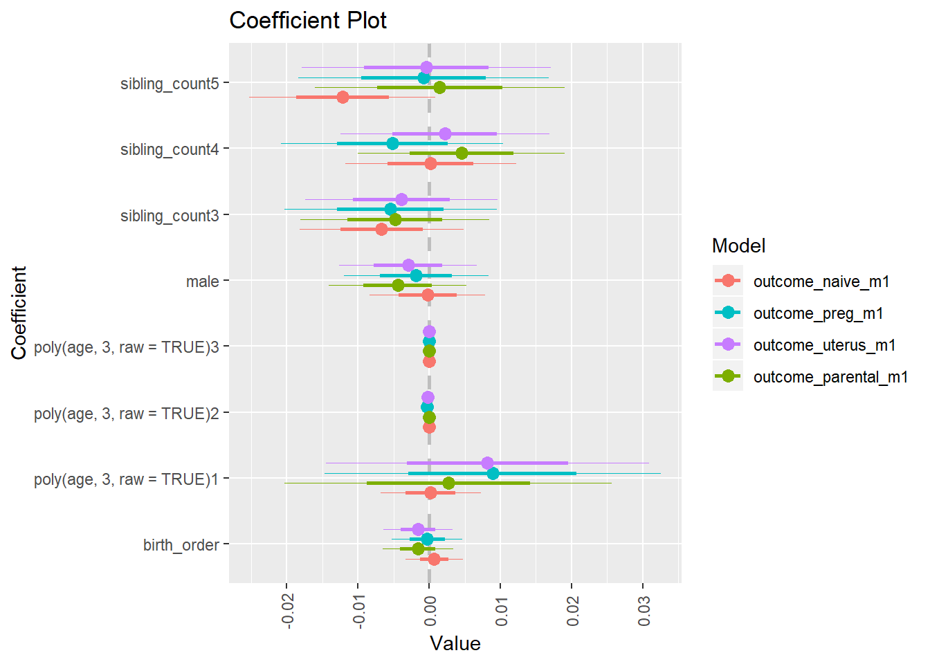
Sector_Finance, insurance, real estate and business services
birthorder <- birthorder %>% mutate(outcome = `Sector_Finance, insurance, real estate and business services`)
model = lmer(outcome ~ birth_order + poly(age, 3, raw = TRUE) + male + sibling_count + (1 | mother_pidlink),
data = birthorder)
compare_birthorder_specs(model)Naive birth order
outcome_naive_m1 <- update(m2_birthorder_linear, data = birthorder %>%
mutate(sibling_count = sibling_count_naive_factor,
birth_order_nonlinear = birthorder_naive_factor,
birth_order = birthorder_naive,
count_birth_order = count_birthorder_naive) %>%
filter(sibling_count != "1"))
compare_models_markdown(outcome_naive_m1)Basic Model
Model Summary
m1_covariates_only <- update(m2_birthorder_linear, formula = . ~ . - birth_order)
tidy(m1_covariates_only, conf.int = T, conf.level = 0.995)| effect | group | term | estimate | std.error | statistic | df | p.value | conf.low | conf.high |
|---|---|---|---|---|---|---|---|---|---|
| fixed | NA | (Intercept) | -0.0952 | 0.1248 | -0.7629 | 4271 | 0.4456 | -0.4455 | 0.2551 |
| fixed | NA | poly(age, 3, raw = TRUE)1 | 0.02768 | 0.01111 | 2.492 | 4156 | 0.01275 | -0.003503 | 0.05886 |
| fixed | NA | poly(age, 3, raw = TRUE)2 | -0.0007003 | 0.0003078 | -2.275 | 4024 | 0.02294 | -0.001564 | 0.0001637 |
| fixed | NA | poly(age, 3, raw = TRUE)3 | 0.000005302 | 0.000002685 | 1.975 | 3905 | 0.04838 | -0.000002235 | 0.00001284 |
| fixed | NA | male | 0.05929 | 0.01266 | 4.683 | 4573 | 0.000002906 | 0.02375 | 0.09483 |
| fixed | NA | sibling_count3 | -0.009161 | 0.01833 | -0.4998 | 3296 | 0.6173 | -0.06062 | 0.04229 |
| fixed | NA | sibling_count4 | -0.02675 | 0.01856 | -1.442 | 3068 | 0.1495 | -0.07884 | 0.02534 |
| fixed | NA | sibling_count5 | -0.0301 | 0.01932 | -1.558 | 2846 | 0.1193 | -0.08434 | 0.02413 |
| ran_pars | mother_pidlink | sd__(Intercept) | 0.1521 | NA | NA | NA | NA | NA | NA |
| ran_pars | Residual | sd__Observation | 0.4017 | NA | NA | NA | NA | NA | NA |
Coefficient Plot
plot(allEffects(m1_covariates_only, confidence.level = 0.995))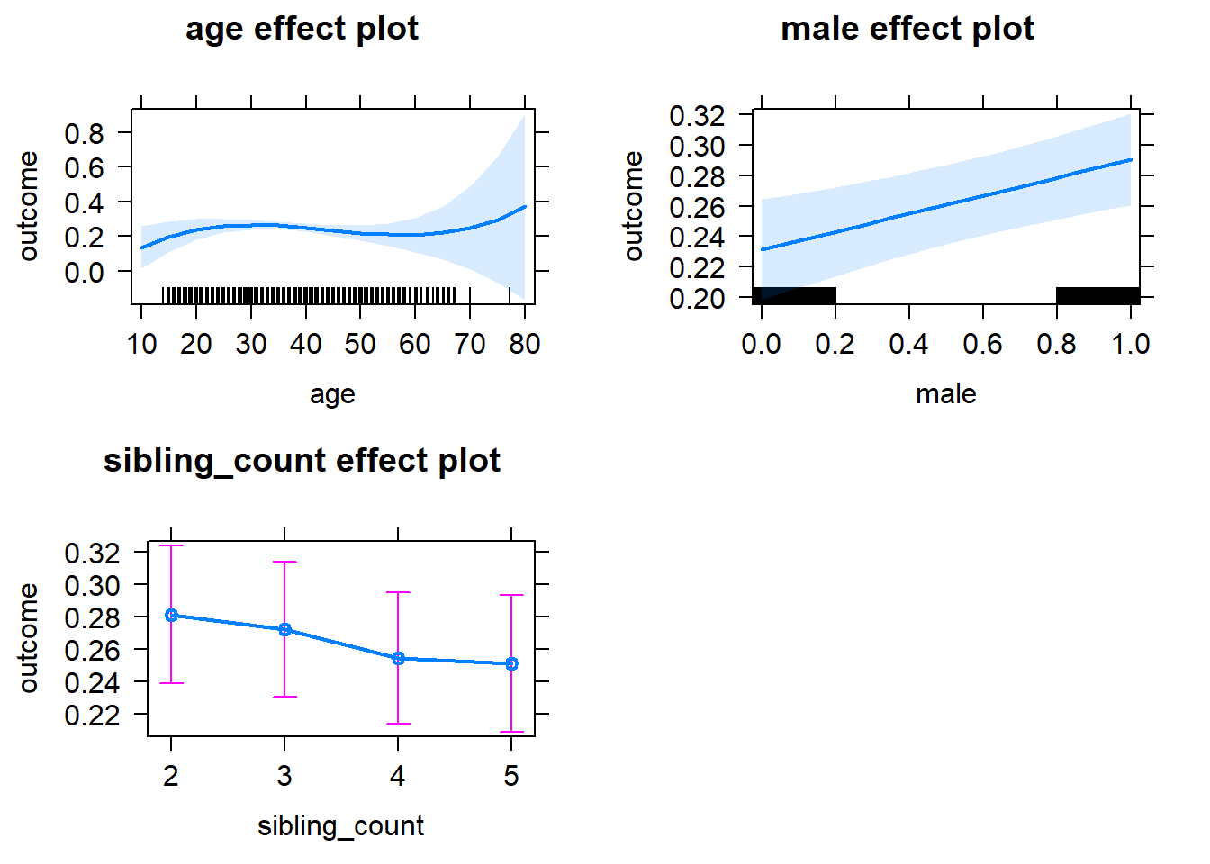
Add Birth Order Linear
Model Summary
tidy(m2_birthorder_linear, conf.int = T, conf.level = 0.995)| effect | group | term | estimate | std.error | statistic | df | p.value | conf.low | conf.high |
|---|---|---|---|---|---|---|---|---|---|
| fixed | NA | (Intercept) | -0.09684 | 0.1248 | -0.776 | 4271 | 0.4378 | -0.4471 | 0.2535 |
| fixed | NA | birth_order | -0.006404 | 0.006212 | -1.031 | 4040 | 0.3027 | -0.02384 | 0.01103 |
| fixed | NA | poly(age, 3, raw = TRUE)1 | 0.02868 | 0.01115 | 2.572 | 4157 | 0.01015 | -0.002621 | 0.05997 |
| fixed | NA | poly(age, 3, raw = TRUE)2 | -0.0007255 | 0.0003087 | -2.35 | 4015 | 0.01882 | -0.001592 | 0.0001411 |
| fixed | NA | poly(age, 3, raw = TRUE)3 | 0.000005474 | 0.00000269 | 2.035 | 3896 | 0.04194 | -0.000002077 | 0.00001303 |
| fixed | NA | male | 0.0592 | 0.01266 | 4.676 | 4572 | 0.000003013 | 0.02366 | 0.09474 |
| fixed | NA | sibling_count3 | -0.006781 | 0.01847 | -0.3671 | 3381 | 0.7136 | -0.05863 | 0.04507 |
| fixed | NA | sibling_count4 | -0.02162 | 0.01921 | -1.125 | 3415 | 0.2605 | -0.07555 | 0.03231 |
| fixed | NA | sibling_count5 | -0.02195 | 0.02087 | -1.052 | 3538 | 0.293 | -0.08053 | 0.03663 |
| ran_pars | mother_pidlink | sd__(Intercept) | 0.1518 | NA | NA | NA | NA | NA | NA |
| ran_pars | Residual | sd__Observation | 0.4018 | NA | NA | NA | NA | NA | NA |
Coefficient Plot
plot_birthorder2(m2_birthorder_linear, separate = FALSE)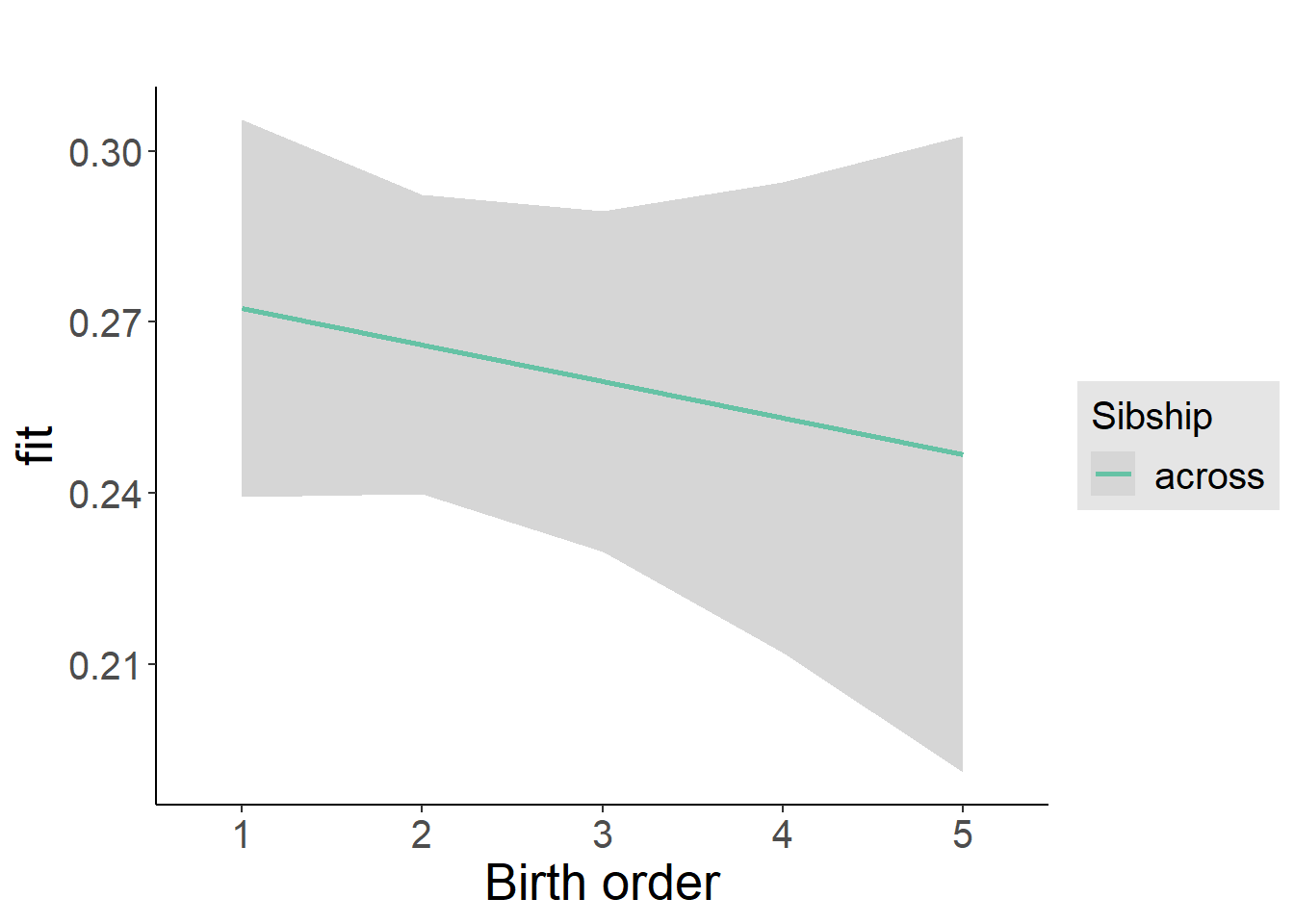
Add Birth Order Factor
Model Summary
m3_birthorder_nonlinear = update(m1_covariates_only, formula = . ~ . + birth_order_nonlinear)
tidy(m3_birthorder_nonlinear, conf.int = T, conf.level = 0.995)| effect | group | term | estimate | std.error | statistic | df | p.value | conf.low | conf.high |
|---|---|---|---|---|---|---|---|---|---|
| fixed | NA | (Intercept) | -0.105 | 0.1252 | -0.8384 | 4275 | 0.4018 | -0.4563 | 0.2464 |
| fixed | NA | poly(age, 3, raw = TRUE)1 | 0.02888 | 0.01115 | 2.589 | 4151 | 0.009654 | -0.00243 | 0.06018 |
| fixed | NA | poly(age, 3, raw = TRUE)2 | -0.0007299 | 0.0003089 | -2.363 | 4004 | 0.01818 | -0.001597 | 0.0001372 |
| fixed | NA | poly(age, 3, raw = TRUE)3 | 0.000005501 | 0.000002693 | 2.043 | 3879 | 0.04111 | -0.000002057 | 0.00001306 |
| fixed | NA | male | 0.05957 | 0.01267 | 4.703 | 4570 | 0.000002641 | 0.02401 | 0.09513 |
| fixed | NA | sibling_count3 | -0.008454 | 0.01878 | -0.4502 | 3530 | 0.6526 | -0.06116 | 0.04426 |
| fixed | NA | sibling_count4 | -0.01924 | 0.01955 | -0.9846 | 3577 | 0.3249 | -0.07411 | 0.03562 |
| fixed | NA | sibling_count5 | -0.02423 | 0.02107 | -1.15 | 3631 | 0.2501 | -0.08338 | 0.03491 |
| fixed | NA | birth_order_nonlinear2 | -0.009479 | 0.01497 | -0.6331 | 3965 | 0.5267 | -0.05151 | 0.03255 |
| fixed | NA | birth_order_nonlinear3 | -0.006589 | 0.01897 | -0.3473 | 3895 | 0.7284 | -0.05985 | 0.04667 |
| fixed | NA | birth_order_nonlinear4 | -0.04194 | 0.02478 | -1.692 | 3827 | 0.09064 | -0.1115 | 0.02762 |
| fixed | NA | birth_order_nonlinear5 | 0.0004922 | 0.03578 | 0.01376 | 3878 | 0.989 | -0.09993 | 0.1009 |
| ran_pars | mother_pidlink | sd__(Intercept) | 0.1513 | NA | NA | NA | NA | NA | NA |
| ran_pars | Residual | sd__Observation | 0.402 | NA | NA | NA | NA | NA | NA |
Coefficient Plot
plot_birthorder(m3_birthorder_nonlinear, separate = FALSE)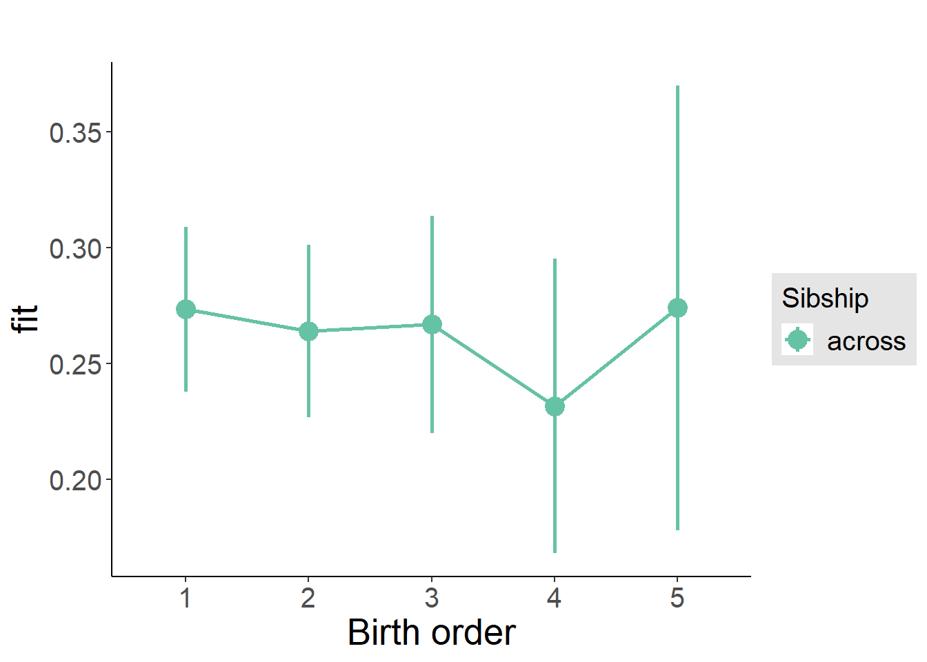
Add Interaction
Model Summary
m4_interaction = update(m3_birthorder_nonlinear, formula = . ~ . - birth_order_nonlinear - sibling_count + count_birth_order)
tidy(m4_interaction, conf.int = T, conf.level = 0.995)| effect | group | term | estimate | std.error | statistic | df | p.value | conf.low | conf.high |
|---|---|---|---|---|---|---|---|---|---|
| fixed | NA | (Intercept) | -0.1004 | 0.1254 | -0.8004 | 4280 | 0.4235 | -0.4523 | 0.2516 |
| fixed | NA | poly(age, 3, raw = TRUE)1 | 0.02951 | 0.01116 | 2.644 | 4149 | 0.008233 | -0.001824 | 0.06085 |
| fixed | NA | poly(age, 3, raw = TRUE)2 | -0.0007396 | 0.0003091 | -2.393 | 4003 | 0.01675 | -0.001607 | 0.0001279 |
| fixed | NA | poly(age, 3, raw = TRUE)3 | 0.000005515 | 0.000002694 | 2.047 | 3877 | 0.04069 | -0.000002046 | 0.00001308 |
| fixed | NA | male | 0.06008 | 0.01267 | 4.742 | 4562 | 0.000002184 | 0.02451 | 0.09565 |
| fixed | NA | count_birth_order2/2 | -0.0483 | 0.02547 | -1.896 | 3910 | 0.058 | -0.1198 | 0.0232 |
| fixed | NA | count_birth_order1/3 | -0.01707 | 0.02459 | -0.6942 | 4613 | 0.4876 | -0.0861 | 0.05196 |
| fixed | NA | count_birth_order2/3 | -0.0285 | 0.02736 | -1.042 | 4623 | 0.2977 | -0.1053 | 0.04831 |
| fixed | NA | count_birth_order3/3 | -0.04638 | 0.03009 | -1.541 | 4625 | 0.1233 | -0.1308 | 0.03809 |
| fixed | NA | count_birth_order1/4 | -0.0567 | 0.02708 | -2.094 | 4624 | 0.03629 | -0.1327 | 0.0193 |
| fixed | NA | count_birth_order2/4 | -0.0309 | 0.02905 | -1.064 | 4625 | 0.2874 | -0.1124 | 0.05063 |
| fixed | NA | count_birth_order3/4 | -0.03242 | 0.03065 | -1.058 | 4624 | 0.2902 | -0.1184 | 0.0536 |
| fixed | NA | count_birth_order4/4 | -0.06348 | 0.03304 | -1.922 | 4621 | 0.05472 | -0.1562 | 0.02925 |
| fixed | NA | count_birth_order1/5 | -0.05637 | 0.03052 | -1.847 | 4623 | 0.06482 | -0.142 | 0.0293 |
| fixed | NA | count_birth_order2/5 | -0.02747 | 0.03243 | -0.8471 | 4620 | 0.397 | -0.1185 | 0.06355 |
| fixed | NA | count_birth_order3/5 | -0.03353 | 0.03411 | -0.9832 | 4613 | 0.3255 | -0.1293 | 0.0622 |
| fixed | NA | count_birth_order4/5 | -0.09669 | 0.03602 | -2.685 | 4593 | 0.007288 | -0.1978 | 0.00441 |
| fixed | NA | count_birth_order5/5 | -0.03857 | 0.03612 | -1.068 | 4609 | 0.2857 | -0.14 | 0.06283 |
| ran_pars | mother_pidlink | sd__(Intercept) | 0.1515 | NA | NA | NA | NA | NA | NA |
| ran_pars | Residual | sd__Observation | 0.402 | NA | NA | NA | NA | NA | NA |
Coefficient Plot
plot_birthorder(m4_interaction)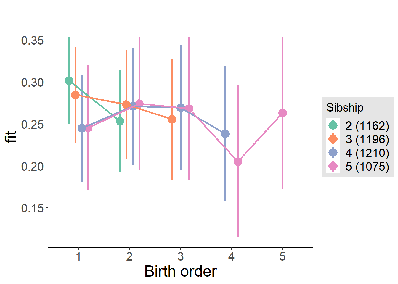
Model Comparison
###### Model 1 - Model 2
anova(m1_covariates_only, m2_birthorder_linear, m3_birthorder_nonlinear, m4_interaction)## refitting model(s) with ML (instead of REML)| Df | AIC | BIC | logLik | deviance | Chisq | Chi Df | Pr(>Chisq) |
|---|---|---|---|---|---|---|---|
| 10 | 5313 | 5378 | -2647 | 5293 | NA | NA | NA |
| 11 | 5314 | 5385 | -2646 | 5292 | 1.066 | 1 | 0.3019 |
| 14 | 5318 | 5408 | -2645 | 5290 | 2.037 | 3 | 0.5648 |
| 20 | 5324 | 5453 | -2642 | 5284 | 6.17 | 6 | 0.4045 |
Maternal birth order
outcome_uterus_m1 <- update(m2_birthorder_linear, data = birthorder %>%
mutate(sibling_count = sibling_count_uterus_alive_factor,
birth_order_nonlinear = birthorder_uterus_alive_factor,
birth_order = birthorder_uterus_alive,
count_birth_order = count_birthorder_uterus_alive) %>%
filter(sibling_count != "1"))
compare_models_markdown(outcome_uterus_m1)Basic Model
Model Summary
m1_covariates_only <- update(m2_birthorder_linear, formula = . ~ . - birth_order)
tidy(m1_covariates_only, conf.int = T, conf.level = 0.995)| effect | group | term | estimate | std.error | statistic | df | p.value | conf.low | conf.high |
|---|---|---|---|---|---|---|---|---|---|
| fixed | NA | (Intercept) | -0.5641 | 0.3703 | -1.523 | 2623 | 0.1278 | -1.604 | 0.4753 |
| fixed | NA | poly(age, 3, raw = TRUE)1 | 0.08228 | 0.04098 | 2.008 | 2623 | 0.04478 | -0.03276 | 0.1973 |
| fixed | NA | poly(age, 3, raw = TRUE)2 | -0.002539 | 0.001452 | -1.749 | 2622 | 0.08041 | -0.006614 | 0.001536 |
| fixed | NA | poly(age, 3, raw = TRUE)3 | 0.00002533 | 0.00001647 | 1.538 | 2620 | 0.1242 | -0.0000209 | 0.00007155 |
| fixed | NA | male | 0.04971 | 0.01742 | 2.855 | 2630 | 0.004344 | 0.0008273 | 0.0986 |
| fixed | NA | sibling_count3 | -0.03371 | 0.02417 | -1.394 | 2085 | 0.1633 | -0.1016 | 0.03415 |
| fixed | NA | sibling_count4 | -0.04468 | 0.02501 | -1.787 | 1891 | 0.07414 | -0.1149 | 0.02551 |
| fixed | NA | sibling_count5 | -0.09709 | 0.02785 | -3.486 | 1617 | 0.000503 | -0.1753 | -0.01892 |
| ran_pars | mother_pidlink | sd__(Intercept) | 0.1114 | NA | NA | NA | NA | NA | NA |
| ran_pars | Residual | sd__Observation | 0.427 | NA | NA | NA | NA | NA | NA |
Coefficient Plot
plot(allEffects(m1_covariates_only, confidence.level = 0.995))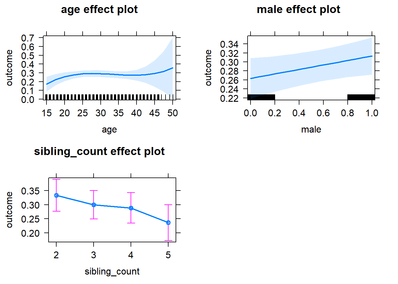
Add Birth Order Linear
Model Summary
tidy(m2_birthorder_linear, conf.int = T, conf.level = 0.995)| effect | group | term | estimate | std.error | statistic | df | p.value | conf.low | conf.high |
|---|---|---|---|---|---|---|---|---|---|
| fixed | NA | (Intercept) | -0.5634 | 0.3703 | -1.521 | 2622 | 0.1283 | -1.603 | 0.4762 |
| fixed | NA | birth_order | -0.004376 | 0.00879 | -0.4979 | 2499 | 0.6186 | -0.02905 | 0.0203 |
| fixed | NA | poly(age, 3, raw = TRUE)1 | 0.0827 | 0.041 | 2.017 | 2621 | 0.04377 | -0.03238 | 0.1978 |
| fixed | NA | poly(age, 3, raw = TRUE)2 | -0.002546 | 0.001452 | -1.754 | 2620 | 0.07957 | -0.006622 | 0.001529 |
| fixed | NA | poly(age, 3, raw = TRUE)3 | 0.0000253 | 0.00001647 | 1.536 | 2619 | 0.1246 | -0.00002093 | 0.00007153 |
| fixed | NA | male | 0.0497 | 0.01742 | 2.854 | 2629 | 0.004357 | 0.0008102 | 0.0986 |
| fixed | NA | sibling_count3 | -0.03164 | 0.02453 | -1.29 | 2119 | 0.1972 | -0.1005 | 0.03721 |
| fixed | NA | sibling_count4 | -0.04021 | 0.02657 | -1.513 | 2023 | 0.1304 | -0.1148 | 0.03438 |
| fixed | NA | sibling_count5 | -0.08963 | 0.03163 | -2.833 | 1953 | 0.004653 | -0.1784 | -0.000833 |
| ran_pars | mother_pidlink | sd__(Intercept) | 0.1113 | NA | NA | NA | NA | NA | NA |
| ran_pars | Residual | sd__Observation | 0.427 | NA | NA | NA | NA | NA | NA |
Coefficient Plot
plot_birthorder2(m2_birthorder_linear, separate = FALSE)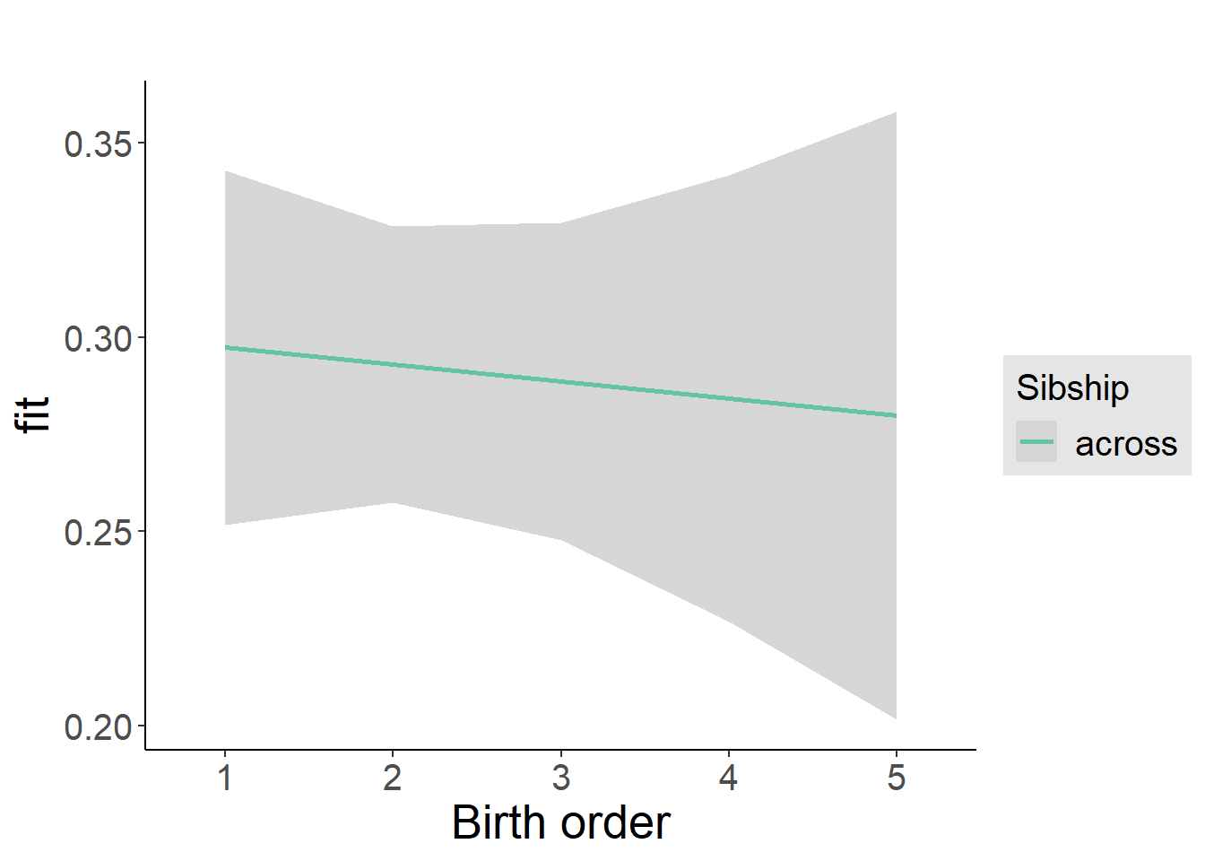
Add Birth Order Factor
Model Summary
m3_birthorder_nonlinear = update(m1_covariates_only, formula = . ~ . + birth_order_nonlinear)
tidy(m3_birthorder_nonlinear, conf.int = T, conf.level = 0.995)| effect | group | term | estimate | std.error | statistic | df | p.value | conf.low | conf.high |
|---|---|---|---|---|---|---|---|---|---|
| fixed | NA | (Intercept) | -0.541 | 0.371 | -1.458 | 2618 | 0.1449 | -1.582 | 0.5003 |
| fixed | NA | poly(age, 3, raw = TRUE)1 | 0.0795 | 0.04105 | 1.937 | 2618 | 0.05287 | -0.03572 | 0.1947 |
| fixed | NA | poly(age, 3, raw = TRUE)2 | -0.002436 | 0.001454 | -1.676 | 2617 | 0.09389 | -0.006516 | 0.001644 |
| fixed | NA | poly(age, 3, raw = TRUE)3 | 0.00002412 | 0.00001649 | 1.463 | 2616 | 0.1436 | -0.00002216 | 0.0000704 |
| fixed | NA | male | 0.04944 | 0.01743 | 2.837 | 2626 | 0.004588 | 0.0005227 | 0.09835 |
| fixed | NA | sibling_count3 | -0.0241 | 0.0249 | -0.968 | 2179 | 0.3332 | -0.09399 | 0.04579 |
| fixed | NA | sibling_count4 | -0.03172 | 0.02693 | -1.178 | 2080 | 0.239 | -0.1073 | 0.04388 |
| fixed | NA | sibling_count5 | -0.09454 | 0.03203 | -2.952 | 1997 | 0.003196 | -0.1844 | -0.004636 |
| fixed | NA | birth_order_nonlinear2 | 0.002414 | 0.02101 | 0.1149 | 2287 | 0.9085 | -0.05655 | 0.06138 |
| fixed | NA | birth_order_nonlinear3 | -0.0408 | 0.0256 | -1.594 | 2339 | 0.1112 | -0.1127 | 0.03107 |
| fixed | NA | birth_order_nonlinear4 | -0.01793 | 0.03409 | -0.5259 | 2409 | 0.599 | -0.1136 | 0.07775 |
| fixed | NA | birth_order_nonlinear5 | 0.05211 | 0.05282 | 0.9865 | 2350 | 0.324 | -0.09617 | 0.2004 |
| ran_pars | mother_pidlink | sd__(Intercept) | 0.1121 | NA | NA | NA | NA | NA | NA |
| ran_pars | Residual | sd__Observation | 0.4267 | NA | NA | NA | NA | NA | NA |
Coefficient Plot
plot_birthorder(m3_birthorder_nonlinear, separate = FALSE)
Add Interaction
Model Summary
m4_interaction = update(m3_birthorder_nonlinear, formula = . ~ . - birth_order_nonlinear - sibling_count + count_birth_order)
tidy(m4_interaction, conf.int = T, conf.level = 0.995)| effect | group | term | estimate | std.error | statistic | df | p.value | conf.low | conf.high |
|---|---|---|---|---|---|---|---|---|---|
| fixed | NA | (Intercept) | -0.5359 | 0.3714 | -1.443 | 2612 | 0.1491 | -1.578 | 0.5066 |
| fixed | NA | poly(age, 3, raw = TRUE)1 | 0.08014 | 0.04109 | 1.95 | 2612 | 0.05123 | -0.0352 | 0.1955 |
| fixed | NA | poly(age, 3, raw = TRUE)2 | -0.002451 | 0.001455 | -1.684 | 2611 | 0.09226 | -0.006537 | 0.001634 |
| fixed | NA | poly(age, 3, raw = TRUE)3 | 0.00002421 | 0.00001651 | 1.466 | 2610 | 0.1426 | -0.00002213 | 0.00007055 |
| fixed | NA | male | 0.05036 | 0.01745 | 2.885 | 2620 | 0.003947 | 0.00136 | 0.09935 |
| fixed | NA | count_birth_order2/2 | -0.03881 | 0.03831 | -1.013 | 2282 | 0.3111 | -0.1464 | 0.06873 |
| fixed | NA | count_birth_order1/3 | -0.04922 | 0.03198 | -1.539 | 2623 | 0.1239 | -0.139 | 0.04055 |
| fixed | NA | count_birth_order2/3 | -0.01473 | 0.03554 | -0.4144 | 2624 | 0.6786 | -0.1145 | 0.08504 |
| fixed | NA | count_birth_order3/3 | -0.0825 | 0.03873 | -2.13 | 2622 | 0.03326 | -0.1912 | 0.02622 |
| fixed | NA | count_birth_order1/4 | -0.05063 | 0.03679 | -1.376 | 2624 | 0.1689 | -0.1539 | 0.05265 |
| fixed | NA | count_birth_order2/4 | -0.05041 | 0.03895 | -1.294 | 2623 | 0.1957 | -0.1597 | 0.05892 |
| fixed | NA | count_birth_order3/4 | -0.09033 | 0.04039 | -2.236 | 2621 | 0.02541 | -0.2037 | 0.02305 |
| fixed | NA | count_birth_order4/4 | -0.03833 | 0.04319 | -0.8876 | 2620 | 0.3748 | -0.1596 | 0.08289 |
| fixed | NA | count_birth_order1/5 | -0.1059 | 0.04858 | -2.18 | 2624 | 0.02936 | -0.2423 | 0.03047 |
| fixed | NA | count_birth_order2/5 | -0.08639 | 0.05227 | -1.653 | 2620 | 0.09851 | -0.2331 | 0.06034 |
| fixed | NA | count_birth_order3/5 | -0.133 | 0.04964 | -2.679 | 2618 | 0.007422 | -0.2724 | 0.006338 |
| fixed | NA | count_birth_order4/5 | -0.1591 | 0.04838 | -3.289 | 2616 | 0.001017 | -0.295 | -0.02334 |
| fixed | NA | count_birth_order5/5 | -0.05616 | 0.0509 | -1.103 | 2612 | 0.2699 | -0.199 | 0.08671 |
| ran_pars | mother_pidlink | sd__(Intercept) | 0.1109 | NA | NA | NA | NA | NA | NA |
| ran_pars | Residual | sd__Observation | 0.4272 | NA | NA | NA | NA | NA | NA |
Coefficient Plot
plot_birthorder(m4_interaction)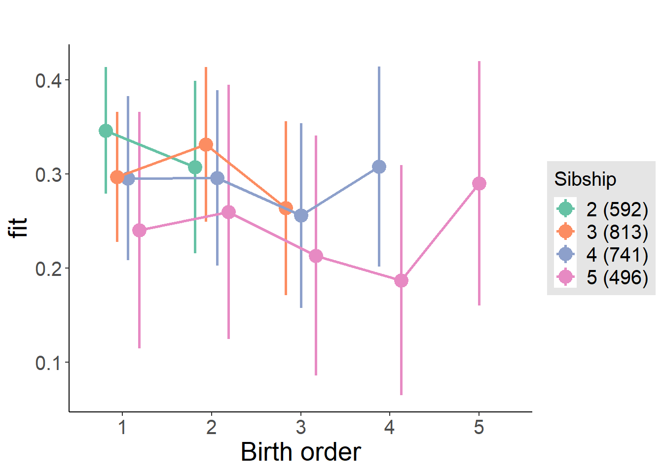
Model Comparison
###### Model 1 - Model 2
anova(m1_covariates_only, m2_birthorder_linear, m3_birthorder_nonlinear, m4_interaction)## refitting model(s) with ML (instead of REML)| Df | AIC | BIC | logLik | deviance | Chisq | Chi Df | Pr(>Chisq) |
|---|---|---|---|---|---|---|---|
| 10 | 3183 | 3242 | -1582 | 3163 | NA | NA | NA |
| 11 | 3185 | 3250 | -1581 | 3163 | 0.2487 | 1 | 0.618 |
| 14 | 3186 | 3269 | -1579 | 3158 | 4.646 | 3 | 0.1997 |
| 20 | 3195 | 3312 | -1577 | 3155 | 3.491 | 6 | 0.7452 |
Maternal pregnancy order
outcome_preg_m1 <- update(m2_birthorder_linear, data = birthorder %>%
mutate(sibling_count = sibling_count_uterus_preg_factor,
birth_order_nonlinear = birthorder_uterus_preg_factor,
birth_order = birthorder_uterus_preg,
count_birth_order = count_birthorder_uterus_preg
) %>%
filter(sibling_count != "1"))
compare_models_markdown(outcome_preg_m1)Basic Model
Model Summary
m1_covariates_only <- update(m2_birthorder_linear, formula = . ~ . - birth_order)
tidy(m1_covariates_only, conf.int = T, conf.level = 0.995)| effect | group | term | estimate | std.error | statistic | df | p.value | conf.low | conf.high |
|---|---|---|---|---|---|---|---|---|---|
| fixed | NA | (Intercept) | -0.6825 | 0.384 | -1.778 | 2414 | 0.0756 | -1.76 | 0.3953 |
| fixed | NA | poly(age, 3, raw = TRUE)1 | 0.09304 | 0.04252 | 2.188 | 2414 | 0.02876 | -0.02632 | 0.2124 |
| fixed | NA | poly(age, 3, raw = TRUE)2 | -0.002874 | 0.001506 | -1.908 | 2413 | 0.05649 | -0.007102 | 0.001354 |
| fixed | NA | poly(age, 3, raw = TRUE)3 | 0.00002847 | 0.00001709 | 1.666 | 2412 | 0.09582 | -0.0000195 | 0.00007644 |
| fixed | NA | male | 0.05795 | 0.01819 | 3.186 | 2413 | 0.001461 | 0.006892 | 0.109 |
| fixed | NA | sibling_count3 | -0.01966 | 0.02661 | -0.7388 | 1954 | 0.4601 | -0.09436 | 0.05504 |
| fixed | NA | sibling_count4 | -0.03128 | 0.02693 | -1.162 | 1842 | 0.2455 | -0.1069 | 0.04431 |
| fixed | NA | sibling_count5 | -0.07082 | 0.02839 | -2.494 | 1683 | 0.01272 | -0.1505 | 0.008883 |
| ran_pars | mother_pidlink | sd__(Intercept) | 0.1233 | NA | NA | NA | NA | NA | NA |
| ran_pars | Residual | sd__Observation | 0.4242 | NA | NA | NA | NA | NA | NA |
Coefficient Plot
plot(allEffects(m1_covariates_only, confidence.level = 0.995))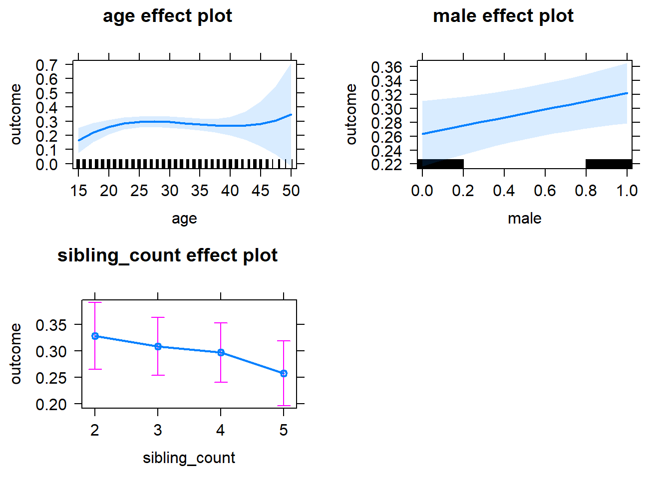
Add Birth Order Linear
Model Summary
tidy(m2_birthorder_linear, conf.int = T, conf.level = 0.995)| effect | group | term | estimate | std.error | statistic | df | p.value | conf.low | conf.high |
|---|---|---|---|---|---|---|---|---|---|
| fixed | NA | (Intercept) | -0.6803 | 0.3841 | -1.771 | 2413 | 0.07666 | -1.758 | 0.3979 |
| fixed | NA | birth_order | -0.00328 | 0.008915 | -0.3679 | 2339 | 0.713 | -0.0283 | 0.02174 |
| fixed | NA | poly(age, 3, raw = TRUE)1 | 0.09322 | 0.04253 | 2.192 | 2412 | 0.02849 | -0.02617 | 0.2126 |
| fixed | NA | poly(age, 3, raw = TRUE)2 | -0.002876 | 0.001507 | -1.909 | 2412 | 0.05635 | -0.007105 | 0.001353 |
| fixed | NA | poly(age, 3, raw = TRUE)3 | 0.00002842 | 0.00001709 | 1.663 | 2411 | 0.09646 | -0.00001956 | 0.0000764 |
| fixed | NA | male | 0.05785 | 0.01819 | 3.18 | 2412 | 0.001491 | 0.006786 | 0.1089 |
| fixed | NA | sibling_count3 | -0.0181 | 0.02695 | -0.6715 | 1973 | 0.502 | -0.09375 | 0.05756 |
| fixed | NA | sibling_count4 | -0.02819 | 0.02822 | -0.9991 | 1919 | 0.3179 | -0.1074 | 0.05101 |
| fixed | NA | sibling_count5 | -0.06558 | 0.03177 | -2.065 | 1913 | 0.03909 | -0.1548 | 0.02358 |
| ran_pars | mother_pidlink | sd__(Intercept) | 0.1232 | NA | NA | NA | NA | NA | NA |
| ran_pars | Residual | sd__Observation | 0.4243 | NA | NA | NA | NA | NA | NA |
Coefficient Plot
plot_birthorder2(m2_birthorder_linear, separate = FALSE)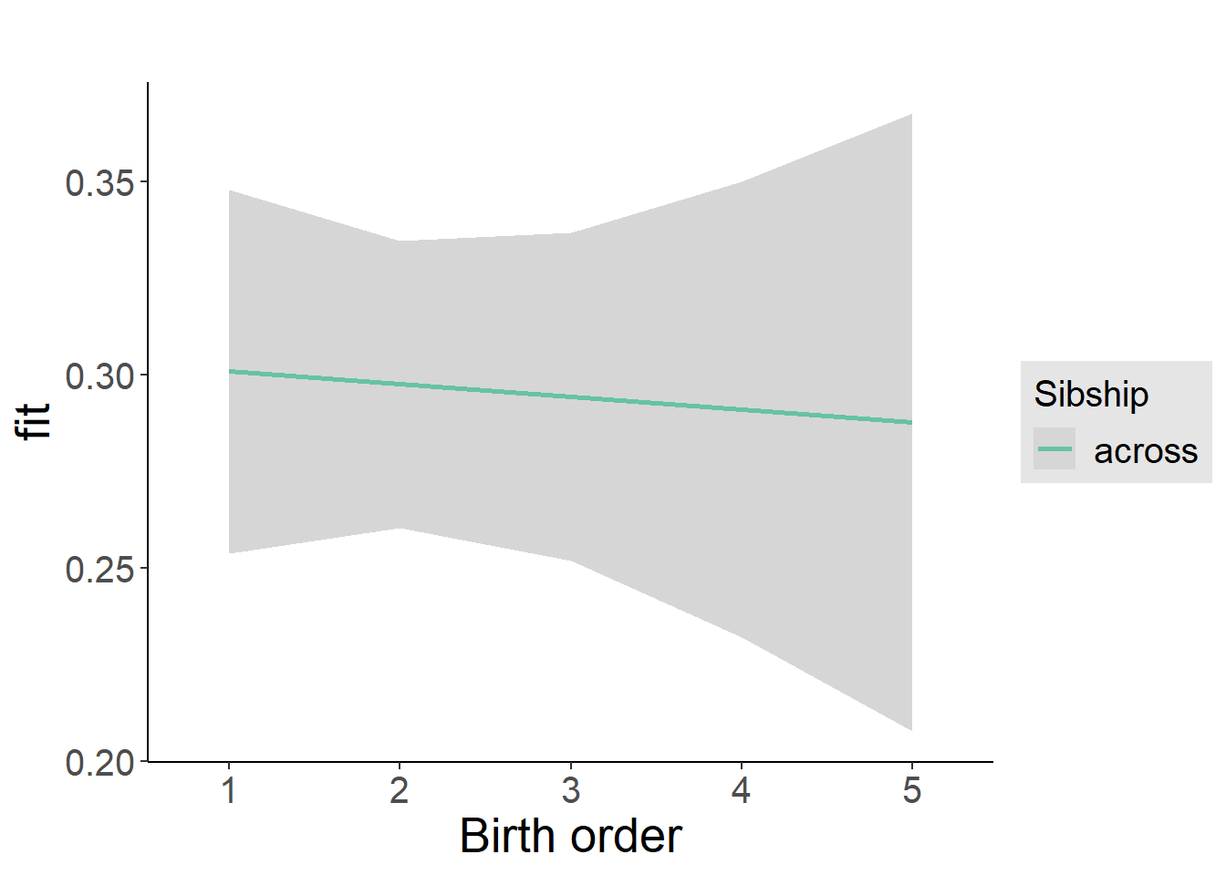
Add Birth Order Factor
Model Summary
m3_birthorder_nonlinear = update(m1_covariates_only, formula = . ~ . + birth_order_nonlinear)
tidy(m3_birthorder_nonlinear, conf.int = T, conf.level = 0.995)| effect | group | term | estimate | std.error | statistic | df | p.value | conf.low | conf.high |
|---|---|---|---|---|---|---|---|---|---|
| fixed | NA | (Intercept) | -0.6344 | 0.3848 | -1.649 | 2408 | 0.09935 | -1.715 | 0.4458 |
| fixed | NA | poly(age, 3, raw = TRUE)1 | 0.08752 | 0.0426 | 2.054 | 2409 | 0.04006 | -0.03207 | 0.2071 |
| fixed | NA | poly(age, 3, raw = TRUE)2 | -0.00268 | 0.001509 | -1.776 | 2408 | 0.07586 | -0.006916 | 0.001556 |
| fixed | NA | poly(age, 3, raw = TRUE)3 | 0.0000263 | 0.00001712 | 1.536 | 2407 | 0.1246 | -0.00002175 | 0.00007435 |
| fixed | NA | male | 0.05767 | 0.01819 | 3.17 | 2408 | 0.001544 | 0.0066 | 0.1087 |
| fixed | NA | sibling_count3 | -0.008869 | 0.02733 | -0.3245 | 2017 | 0.7456 | -0.0856 | 0.06786 |
| fixed | NA | sibling_count4 | -0.01803 | 0.02857 | -0.6311 | 1960 | 0.5281 | -0.09823 | 0.06217 |
| fixed | NA | sibling_count5 | -0.06864 | 0.03197 | -2.147 | 1936 | 0.03194 | -0.1584 | 0.02111 |
| fixed | NA | birth_order_nonlinear2 | 0.005051 | 0.02173 | 0.2324 | 2096 | 0.8162 | -0.05596 | 0.06606 |
| fixed | NA | birth_order_nonlinear3 | -0.04662 | 0.02678 | -1.741 | 2184 | 0.08184 | -0.1218 | 0.02855 |
| fixed | NA | birth_order_nonlinear4 | -0.0179 | 0.03534 | -0.5064 | 2247 | 0.6127 | -0.1171 | 0.08131 |
| fixed | NA | birth_order_nonlinear5 | 0.06078 | 0.05073 | 1.198 | 2170 | 0.2311 | -0.08164 | 0.2032 |
| ran_pars | mother_pidlink | sd__(Intercept) | 0.1272 | NA | NA | NA | NA | NA | NA |
| ran_pars | Residual | sd__Observation | 0.4229 | NA | NA | NA | NA | NA | NA |
Coefficient Plot
plot_birthorder(m3_birthorder_nonlinear, separate = FALSE)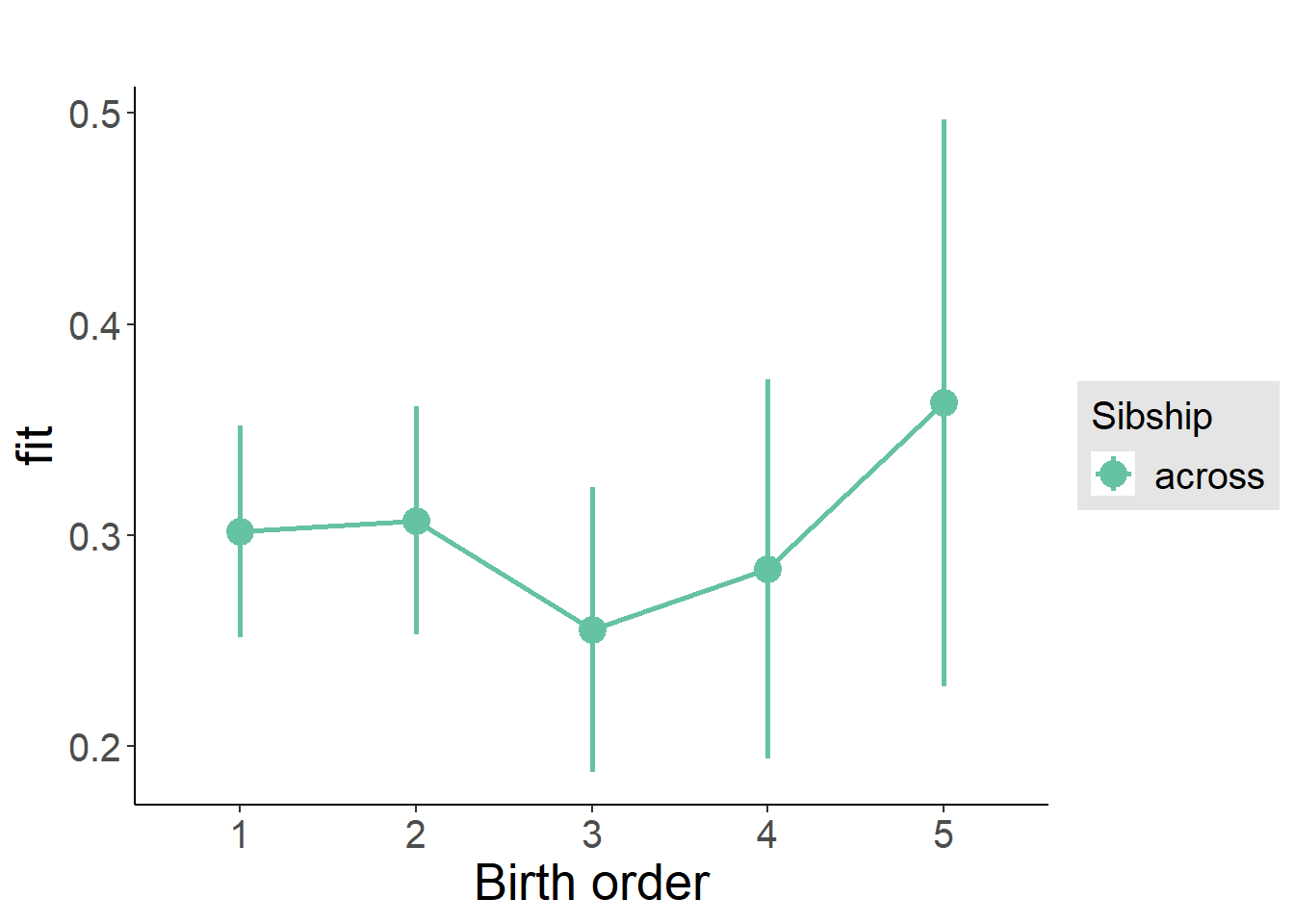
Add Interaction
Model Summary
m4_interaction = update(m3_birthorder_nonlinear, formula = . ~ . - birth_order_nonlinear - sibling_count + count_birth_order)
tidy(m4_interaction, conf.int = T, conf.level = 0.995)| effect | group | term | estimate | std.error | statistic | df | p.value | conf.low | conf.high |
|---|---|---|---|---|---|---|---|---|---|
| fixed | NA | (Intercept) | -0.6039 | 0.3852 | -1.568 | 2402 | 0.117 | -1.685 | 0.4772 |
| fixed | NA | poly(age, 3, raw = TRUE)1 | 0.08648 | 0.04264 | 2.028 | 2402 | 0.04267 | -0.03322 | 0.2062 |
| fixed | NA | poly(age, 3, raw = TRUE)2 | -0.002637 | 0.001511 | -1.746 | 2402 | 0.08098 | -0.006877 | 0.001603 |
| fixed | NA | poly(age, 3, raw = TRUE)3 | 0.00002579 | 0.00001714 | 1.505 | 2401 | 0.1324 | -0.00002231 | 0.00007389 |
| fixed | NA | male | 0.05756 | 0.01823 | 3.158 | 2403 | 0.00161 | 0.006393 | 0.1087 |
| fixed | NA | count_birth_order2/2 | -0.06508 | 0.04191 | -1.553 | 2145 | 0.1206 | -0.1827 | 0.05257 |
| fixed | NA | count_birth_order1/3 | -0.03693 | 0.03539 | -1.043 | 2408 | 0.2968 | -0.1363 | 0.06241 |
| fixed | NA | count_birth_order2/3 | -0.01343 | 0.03851 | -0.3487 | 2409 | 0.7274 | -0.1215 | 0.09466 |
| fixed | NA | count_birth_order3/3 | -0.08976 | 0.04268 | -2.103 | 2406 | 0.03557 | -0.2096 | 0.03005 |
| fixed | NA | count_birth_order1/4 | -0.08182 | 0.03852 | -2.124 | 2408 | 0.03378 | -0.19 | 0.02632 |
| fixed | NA | count_birth_order2/4 | 0.001392 | 0.04053 | 0.03436 | 2409 | 0.9726 | -0.1124 | 0.1152 |
| fixed | NA | count_birth_order3/4 | -0.08294 | 0.04384 | -1.892 | 2405 | 0.05865 | -0.206 | 0.04013 |
| fixed | NA | count_birth_order4/4 | -0.04982 | 0.04756 | -1.047 | 2403 | 0.295 | -0.1833 | 0.08369 |
| fixed | NA | count_birth_order1/5 | -0.06937 | 0.04664 | -1.487 | 2409 | 0.1371 | -0.2003 | 0.06155 |
| fixed | NA | count_birth_order2/5 | -0.1115 | 0.04773 | -2.335 | 2407 | 0.0196 | -0.2455 | 0.02251 |
| fixed | NA | count_birth_order3/5 | -0.1305 | 0.04906 | -2.66 | 2402 | 0.007866 | -0.2682 | 0.007213 |
| fixed | NA | count_birth_order4/5 | -0.1209 | 0.04984 | -2.426 | 2398 | 0.01535 | -0.2608 | 0.01901 |
| fixed | NA | count_birth_order5/5 | -0.0318 | 0.0506 | -0.6285 | 2394 | 0.5298 | -0.1738 | 0.1102 |
| ran_pars | mother_pidlink | sd__(Intercept) | 0.1237 | NA | NA | NA | NA | NA | NA |
| ran_pars | Residual | sd__Observation | 0.4237 | NA | NA | NA | NA | NA | NA |
Coefficient Plot
plot_birthorder(m4_interaction)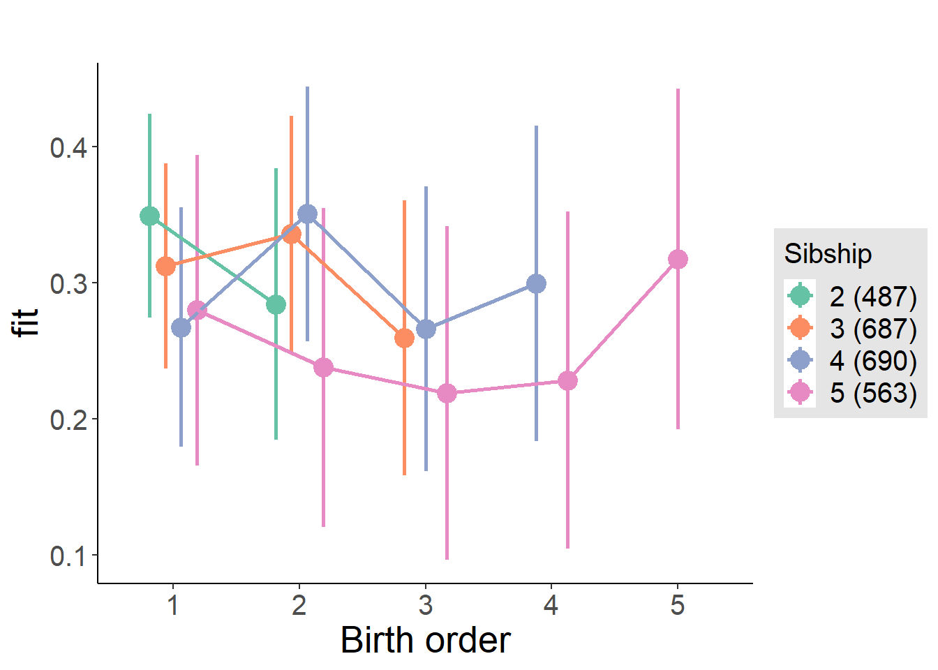
Model Comparison
###### Model 1 - Model 2
anova(m1_covariates_only, m2_birthorder_linear, m3_birthorder_nonlinear, m4_interaction)## refitting model(s) with ML (instead of REML)| Df | AIC | BIC | logLik | deviance | Chisq | Chi Df | Pr(>Chisq) |
|---|---|---|---|---|---|---|---|
| 10 | 2929 | 2987 | -1455 | 2909 | NA | NA | NA |
| 11 | 2931 | 2995 | -1455 | 2909 | 0.1361 | 1 | 0.7122 |
| 14 | 2931 | 3012 | -1451 | 2903 | 6.233 | 3 | 0.1008 |
| 20 | 2935 | 3051 | -1448 | 2895 | 7.511 | 6 | 0.2761 |
Parental full sibling order
outcome_parental_m1 <- update(m2_birthorder_linear, data = birthorder %>%
mutate(sibling_count = sibling_count_genes_factor,
birth_order_nonlinear = birthorder_genes_factor,
birth_order = birthorder_genes,
count_birth_order = count_birthorder_genes
) %>%
filter(sibling_count != "1"))
compare_models_markdown(outcome_parental_m1)Basic Model
Model Summary
m1_covariates_only <- update(m2_birthorder_linear, formula = . ~ . - birth_order)
tidy(m1_covariates_only, conf.int = T, conf.level = 0.995)| effect | group | term | estimate | std.error | statistic | df | p.value | conf.low | conf.high |
|---|---|---|---|---|---|---|---|---|---|
| fixed | NA | (Intercept) | -0.5427 | 0.3734 | -1.453 | 2623 | 0.1462 | -1.591 | 0.5055 |
| fixed | NA | poly(age, 3, raw = TRUE)1 | 0.07979 | 0.04144 | 1.925 | 2623 | 0.05432 | -0.03655 | 0.1961 |
| fixed | NA | poly(age, 3, raw = TRUE)2 | -0.002416 | 0.001471 | -1.642 | 2621 | 0.1007 | -0.006546 | 0.001715 |
| fixed | NA | poly(age, 3, raw = TRUE)3 | 0.00002346 | 0.00001674 | 1.402 | 2619 | 0.1611 | -0.00002352 | 0.00007044 |
| fixed | NA | male | 0.05437 | 0.01739 | 3.127 | 2635 | 0.001783 | 0.005569 | 0.1032 |
| fixed | NA | sibling_count3 | -0.05622 | 0.02361 | -2.381 | 2094 | 0.01737 | -0.1225 | 0.01007 |
| fixed | NA | sibling_count4 | -0.04845 | 0.02475 | -1.957 | 1901 | 0.05045 | -0.1179 | 0.02103 |
| fixed | NA | sibling_count5 | -0.1087 | 0.02832 | -3.838 | 1533 | 0.0001292 | -0.1882 | -0.02919 |
| ran_pars | mother_pidlink | sd__(Intercept) | 0.1054 | NA | NA | NA | NA | NA | NA |
| ran_pars | Residual | sd__Observation | 0.4279 | NA | NA | NA | NA | NA | NA |
Coefficient Plot
plot(allEffects(m1_covariates_only, confidence.level = 0.995))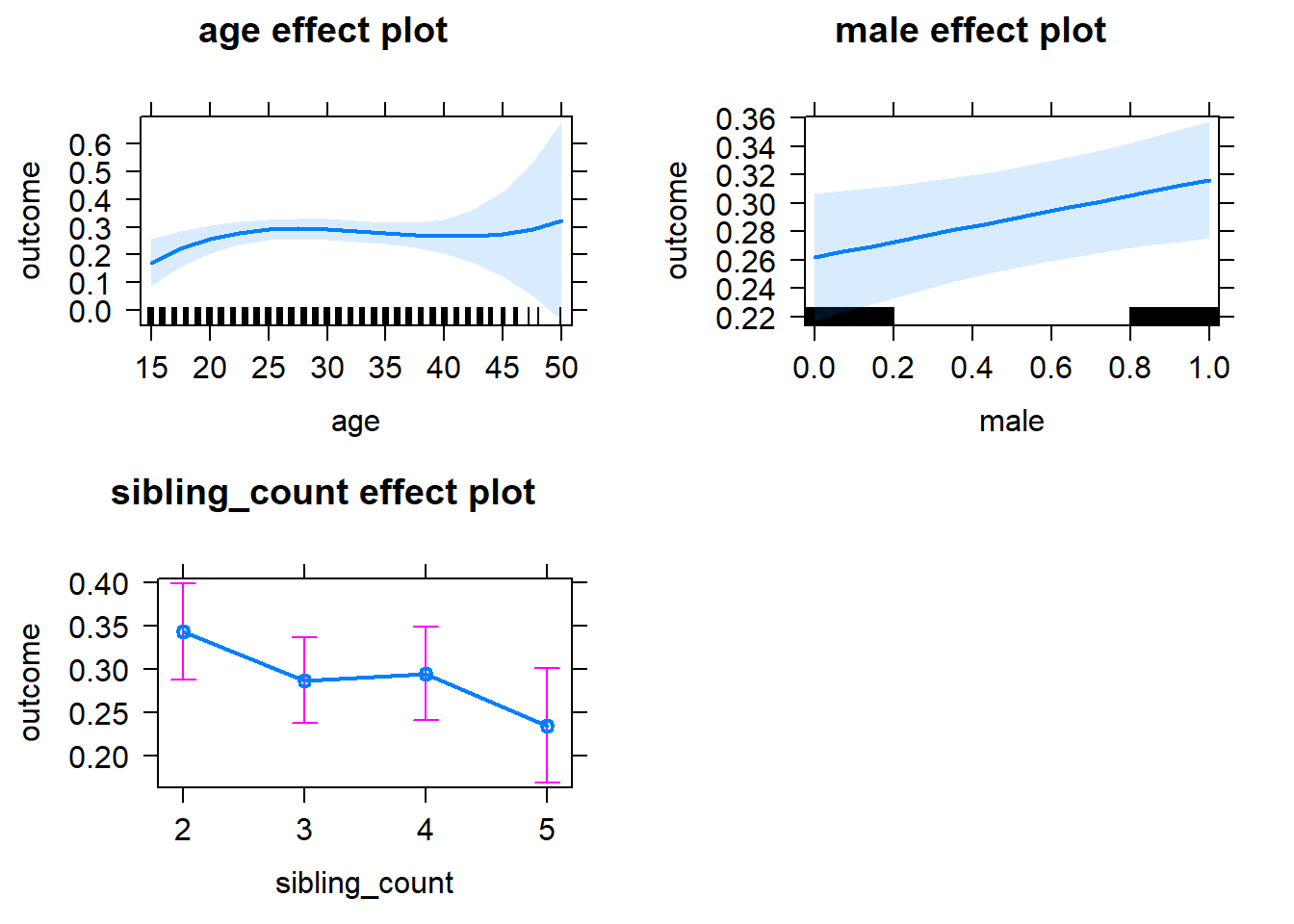
Add Birth Order Linear
Model Summary
tidy(m2_birthorder_linear, conf.int = T, conf.level = 0.995)| effect | group | term | estimate | std.error | statistic | df | p.value | conf.low | conf.high |
|---|---|---|---|---|---|---|---|---|---|
| fixed | NA | (Intercept) | -0.5412 | 0.3735 | -1.449 | 2623 | 0.1474 | -1.589 | 0.5071 |
| fixed | NA | birth_order | -0.007669 | 0.008892 | -0.8625 | 2495 | 0.3885 | -0.03263 | 0.01729 |
| fixed | NA | poly(age, 3, raw = TRUE)1 | 0.08053 | 0.04146 | 1.943 | 2621 | 0.05217 | -0.03583 | 0.1969 |
| fixed | NA | poly(age, 3, raw = TRUE)2 | -0.00243 | 0.001472 | -1.651 | 2620 | 0.09883 | -0.00656 | 0.001701 |
| fixed | NA | poly(age, 3, raw = TRUE)3 | 0.00002343 | 0.00001674 | 1.4 | 2618 | 0.1617 | -0.00002355 | 0.00007041 |
| fixed | NA | male | 0.05427 | 0.01739 | 3.121 | 2634 | 0.001823 | 0.005457 | 0.1031 |
| fixed | NA | sibling_count3 | -0.05255 | 0.02399 | -2.19 | 2128 | 0.02863 | -0.1199 | 0.0148 |
| fixed | NA | sibling_count4 | -0.04069 | 0.02634 | -1.545 | 2041 | 0.1225 | -0.1146 | 0.03324 |
| fixed | NA | sibling_count5 | -0.09613 | 0.03185 | -3.018 | 1845 | 0.002577 | -0.1855 | -0.006726 |
| ran_pars | mother_pidlink | sd__(Intercept) | 0.1052 | NA | NA | NA | NA | NA | NA |
| ran_pars | Residual | sd__Observation | 0.428 | NA | NA | NA | NA | NA | NA |
Coefficient Plot
plot_birthorder2(m2_birthorder_linear, separate = FALSE)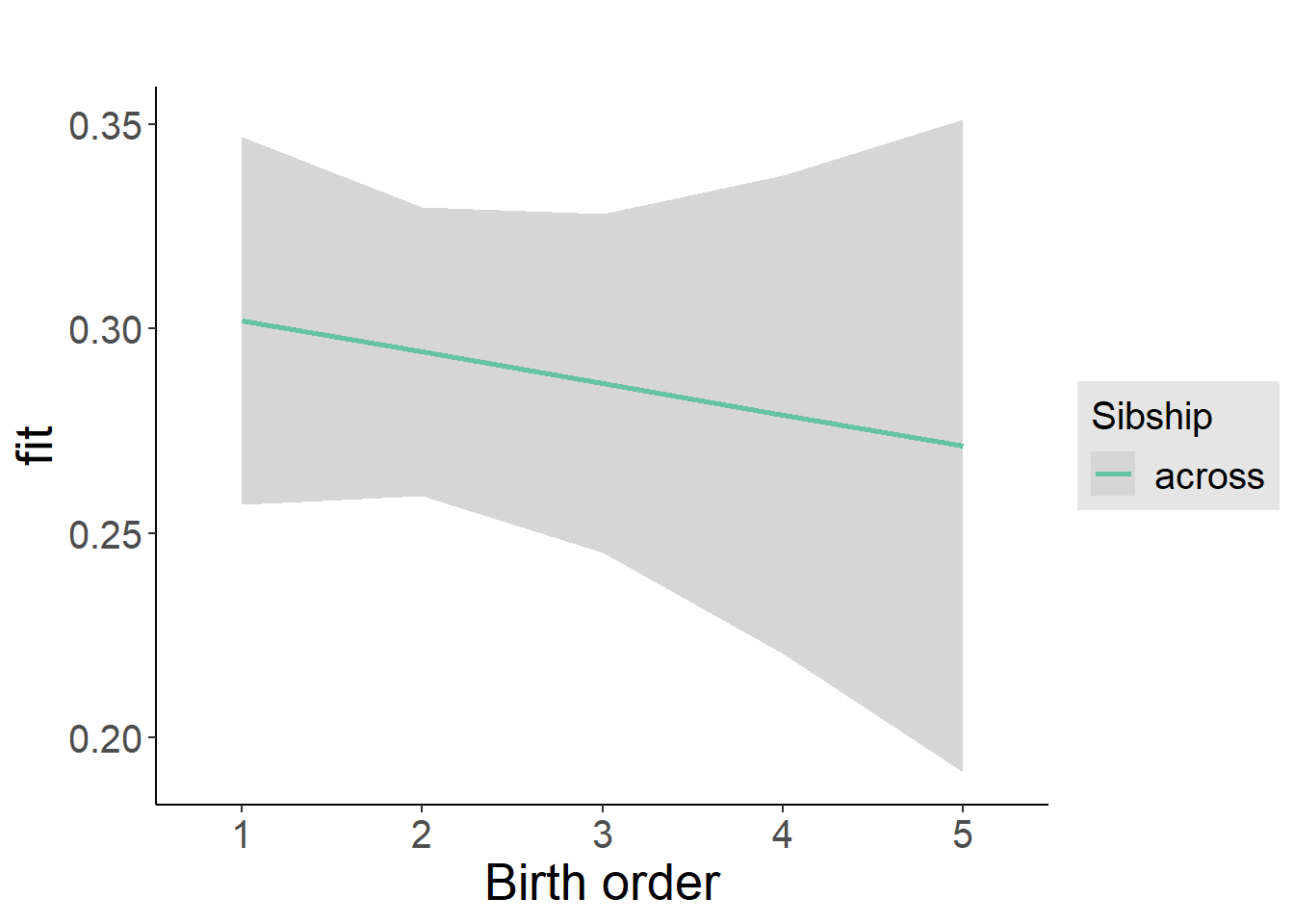
Add Birth Order Factor
Model Summary
m3_birthorder_nonlinear = update(m1_covariates_only, formula = . ~ . + birth_order_nonlinear)
tidy(m3_birthorder_nonlinear, conf.int = T, conf.level = 0.995)| effect | group | term | estimate | std.error | statistic | df | p.value | conf.low | conf.high |
|---|---|---|---|---|---|---|---|---|---|
| fixed | NA | (Intercept) | -0.5204 | 0.374 | -1.391 | 2618 | 0.1642 | -1.57 | 0.5294 |
| fixed | NA | poly(age, 3, raw = TRUE)1 | 0.07746 | 0.0415 | 1.866 | 2618 | 0.06209 | -0.03904 | 0.194 |
| fixed | NA | poly(age, 3, raw = TRUE)2 | -0.00232 | 0.001473 | -1.575 | 2616 | 0.1154 | -0.006455 | 0.001815 |
| fixed | NA | poly(age, 3, raw = TRUE)3 | 0.00002223 | 0.00001675 | 1.327 | 2615 | 0.1847 | -0.0000248 | 0.00006925 |
| fixed | NA | male | 0.05369 | 0.0174 | 3.087 | 2632 | 0.002046 | 0.004863 | 0.1025 |
| fixed | NA | sibling_count3 | -0.04592 | 0.02438 | -1.884 | 2189 | 0.05975 | -0.1143 | 0.02251 |
| fixed | NA | sibling_count4 | -0.03335 | 0.0267 | -1.249 | 2098 | 0.2117 | -0.1083 | 0.04159 |
| fixed | NA | sibling_count5 | -0.105 | 0.03237 | -3.244 | 1901 | 0.001198 | -0.1959 | -0.01415 |
| fixed | NA | birth_order_nonlinear2 | -0.01285 | 0.02078 | -0.6185 | 2290 | 0.5363 | -0.07118 | 0.04547 |
| fixed | NA | birth_order_nonlinear3 | -0.04392 | 0.02553 | -1.72 | 2350 | 0.08548 | -0.1156 | 0.02774 |
| fixed | NA | birth_order_nonlinear4 | -0.03008 | 0.03497 | -0.8602 | 2413 | 0.3898 | -0.1282 | 0.06807 |
| fixed | NA | birth_order_nonlinear5 | 0.05012 | 0.05592 | 0.8964 | 2377 | 0.3701 | -0.1068 | 0.2071 |
| ran_pars | mother_pidlink | sd__(Intercept) | 0.1052 | NA | NA | NA | NA | NA | NA |
| ran_pars | Residual | sd__Observation | 0.4279 | NA | NA | NA | NA | NA | NA |
Coefficient Plot
plot_birthorder(m3_birthorder_nonlinear, separate = FALSE)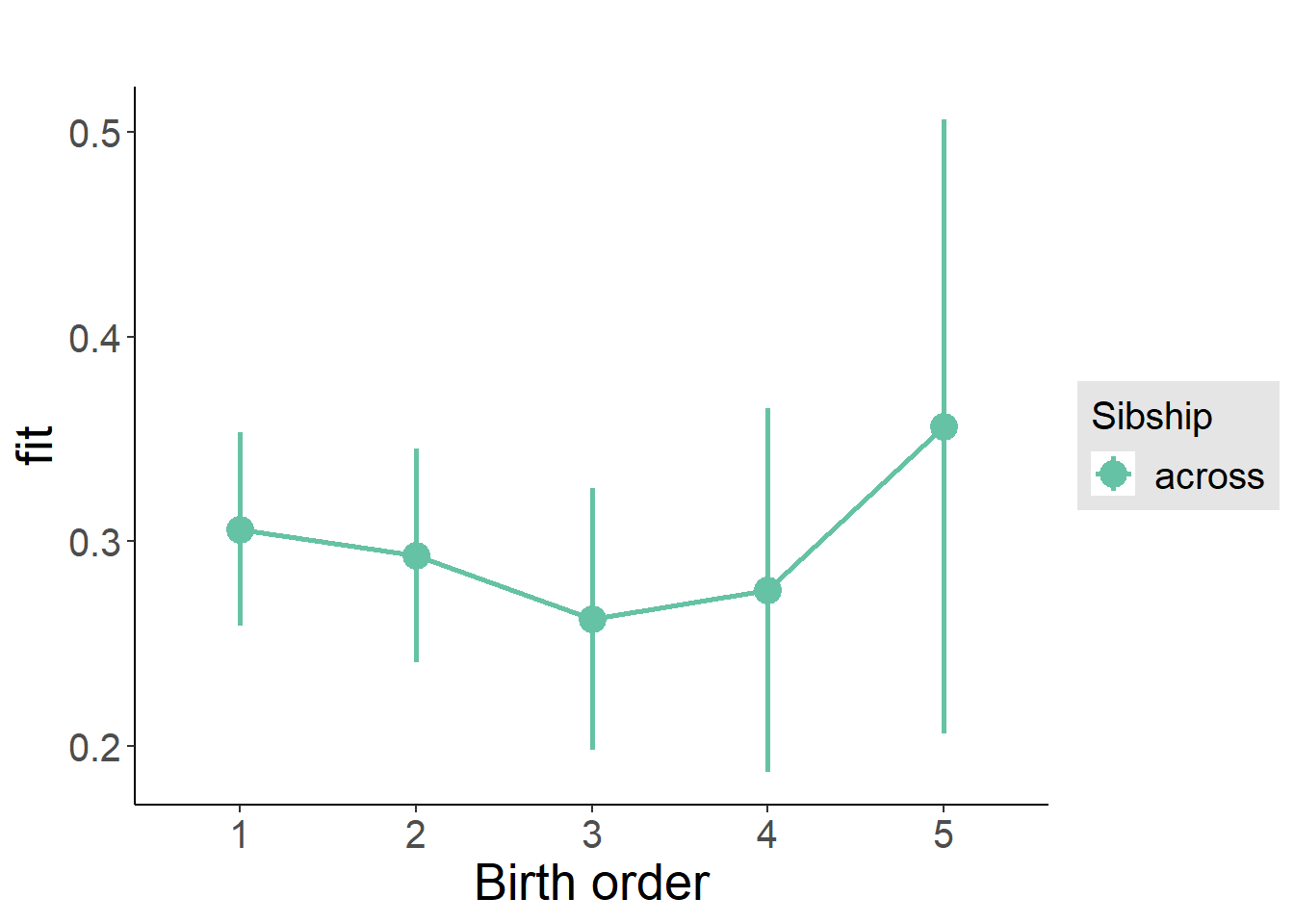
Add Interaction
Model Summary
m4_interaction = update(m3_birthorder_nonlinear, formula = . ~ . - birth_order_nonlinear - sibling_count + count_birth_order)
tidy(m4_interaction, conf.int = T, conf.level = 0.995)| effect | group | term | estimate | std.error | statistic | df | p.value | conf.low | conf.high |
|---|---|---|---|---|---|---|---|---|---|
| fixed | NA | (Intercept) | -0.5216 | 0.3745 | -1.393 | 2612 | 0.1638 | -1.573 | 0.5297 |
| fixed | NA | poly(age, 3, raw = TRUE)1 | 0.07852 | 0.04156 | 1.889 | 2612 | 0.05898 | -0.03815 | 0.1952 |
| fixed | NA | poly(age, 3, raw = TRUE)2 | -0.002356 | 0.001476 | -1.596 | 2610 | 0.1105 | -0.006498 | 0.001786 |
| fixed | NA | poly(age, 3, raw = TRUE)3 | 0.0000226 | 0.00001678 | 1.347 | 2609 | 0.1782 | -0.00002451 | 0.00006971 |
| fixed | NA | male | 0.0543 | 0.01742 | 3.116 | 2625 | 0.001851 | 0.005388 | 0.1032 |
| fixed | NA | count_birth_order2/2 | -0.0402 | 0.03725 | -1.079 | 2286 | 0.2806 | -0.1448 | 0.06437 |
| fixed | NA | count_birth_order1/3 | -0.06318 | 0.03139 | -2.012 | 2627 | 0.04427 | -0.1513 | 0.02494 |
| fixed | NA | count_birth_order2/3 | -0.05513 | 0.03491 | -1.579 | 2628 | 0.1144 | -0.1531 | 0.04286 |
| fixed | NA | count_birth_order3/3 | -0.09972 | 0.03761 | -2.651 | 2625 | 0.008067 | -0.2053 | 0.005858 |
| fixed | NA | count_birth_order1/4 | -0.04047 | 0.03694 | -1.096 | 2628 | 0.2733 | -0.1442 | 0.06321 |
| fixed | NA | count_birth_order2/4 | -0.06359 | 0.03875 | -1.641 | 2627 | 0.1009 | -0.1724 | 0.04519 |
| fixed | NA | count_birth_order3/4 | -0.09215 | 0.04022 | -2.291 | 2625 | 0.02203 | -0.205 | 0.02074 |
| fixed | NA | count_birth_order4/4 | -0.05644 | 0.04365 | -1.293 | 2625 | 0.1961 | -0.179 | 0.06608 |
| fixed | NA | count_birth_order1/5 | -0.124 | 0.04843 | -2.56 | 2628 | 0.01053 | -0.2599 | 0.01198 |
| fixed | NA | count_birth_order2/5 | -0.1018 | 0.05395 | -1.887 | 2624 | 0.0593 | -0.2532 | 0.04965 |
| fixed | NA | count_birth_order3/5 | -0.1439 | 0.05253 | -2.74 | 2622 | 0.006181 | -0.2914 | 0.003508 |
| fixed | NA | count_birth_order4/5 | -0.1673 | 0.05052 | -3.312 | 2620 | 0.0009396 | -0.3092 | -0.0255 |
| fixed | NA | count_birth_order5/5 | -0.06397 | 0.05365 | -1.192 | 2618 | 0.2333 | -0.2146 | 0.08664 |
| ran_pars | mother_pidlink | sd__(Intercept) | 0.1051 | NA | NA | NA | NA | NA | NA |
| ran_pars | Residual | sd__Observation | 0.4283 | NA | NA | NA | NA | NA | NA |
Coefficient Plot
plot_birthorder(m4_interaction)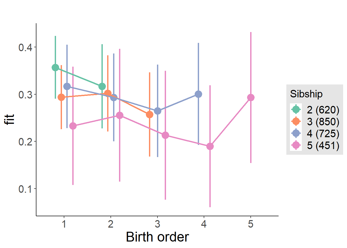
Model Comparison
###### Model 1 - Model 2
anova(m1_covariates_only, m2_birthorder_linear, m3_birthorder_nonlinear, m4_interaction)## refitting model(s) with ML (instead of REML)| Df | AIC | BIC | logLik | deviance | Chisq | Chi Df | Pr(>Chisq) |
|---|---|---|---|---|---|---|---|
| 10 | 3182 | 3241 | -1581 | 3162 | NA | NA | NA |
| 11 | 3184 | 3248 | -1581 | 3162 | 0.7466 | 1 | 0.3875 |
| 14 | 3185 | 3268 | -1579 | 3157 | 4.143 | 3 | 0.2465 |
| 20 | 3196 | 3313 | -1578 | 3156 | 1.874 | 6 | 0.9309 |
Compare birth order specifications
library(coefplot)
multiplot(outcome_naive_m1, outcome_preg_m1, outcome_uterus_m1, outcome_parental_m1, dodgeHeight = 0.6,
intercept = FALSE)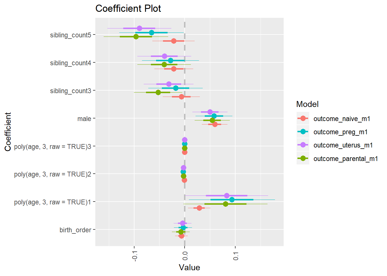
Sector_Manufacturing
birthorder <- birthorder %>% mutate(outcome = Sector_Manufacturing)
model = lmer(outcome ~ birth_order + poly(age, 3, raw = TRUE) + male + sibling_count + (1 | mother_pidlink),
data = birthorder)
compare_birthorder_specs(model)Naive birth order
outcome_naive_m1 <- update(m2_birthorder_linear, data = birthorder %>%
mutate(sibling_count = sibling_count_naive_factor,
birth_order_nonlinear = birthorder_naive_factor,
birth_order = birthorder_naive,
count_birth_order = count_birthorder_naive) %>%
filter(sibling_count != "1"))
compare_models_markdown(outcome_naive_m1)Basic Model
Model Summary
m1_covariates_only <- update(m2_birthorder_linear, formula = . ~ . - birth_order)
tidy(m1_covariates_only, conf.int = T, conf.level = 0.995)| effect | group | term | estimate | std.error | statistic | df | p.value | conf.low | conf.high |
|---|---|---|---|---|---|---|---|---|---|
| fixed | NA | (Intercept) | 0.4453 | 0.1239 | 3.595 | 4256 | 0.000328 | 0.0976 | 0.793 |
| fixed | NA | poly(age, 3, raw = TRUE)1 | -0.009442 | 0.01103 | -0.8562 | 4137 | 0.3919 | -0.04039 | 0.02151 |
| fixed | NA | poly(age, 3, raw = TRUE)2 | 0.00007207 | 0.0003056 | 0.2359 | 4000 | 0.8135 | -0.0007857 | 0.0009298 |
| fixed | NA | poly(age, 3, raw = TRUE)3 | 0.0000006005 | 0.000002666 | 0.2252 | 3877 | 0.8218 | -0.000006884 | 0.000008085 |
| fixed | NA | male | -0.02272 | 0.01255 | -1.81 | 4563 | 0.07036 | -0.05795 | 0.01251 |
| fixed | NA | sibling_count3 | -0.005581 | 0.01821 | -0.3064 | 3230 | 0.7593 | -0.0567 | 0.04554 |
| fixed | NA | sibling_count4 | -0.005379 | 0.01844 | -0.2917 | 3002 | 0.7705 | -0.05714 | 0.04638 |
| fixed | NA | sibling_count5 | 0.0145 | 0.0192 | 0.7549 | 2780 | 0.4504 | -0.03941 | 0.0684 |
| ran_pars | mother_pidlink | sd__(Intercept) | 0.1548 | NA | NA | NA | NA | NA | NA |
| ran_pars | Residual | sd__Observation | 0.3971 | NA | NA | NA | NA | NA | NA |
Coefficient Plot
plot(allEffects(m1_covariates_only, confidence.level = 0.995))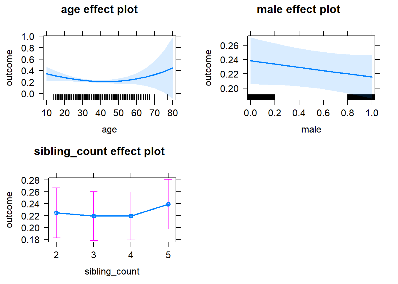
Add Birth Order Linear
Model Summary
tidy(m2_birthorder_linear, conf.int = T, conf.level = 0.995)| effect | group | term | estimate | std.error | statistic | df | p.value | conf.low | conf.high |
|---|---|---|---|---|---|---|---|---|---|
| fixed | NA | (Intercept) | 0.4441 | 0.1239 | 3.585 | 4256 | 0.0003409 | 0.09637 | 0.7918 |
| fixed | NA | birth_order | -0.004553 | 0.006154 | -0.7399 | 3992 | 0.4594 | -0.02183 | 0.01272 |
| fixed | NA | poly(age, 3, raw = TRUE)1 | -0.008725 | 0.01107 | -0.7882 | 4138 | 0.4306 | -0.0398 | 0.02235 |
| fixed | NA | poly(age, 3, raw = TRUE)2 | 0.00005388 | 0.0003065 | 0.1758 | 3991 | 0.8605 | -0.0008066 | 0.0009144 |
| fixed | NA | poly(age, 3, raw = TRUE)3 | 0.0000007249 | 0.000002671 | 0.2713 | 3868 | 0.7861 | -0.000006774 | 0.000008224 |
| fixed | NA | male | -0.02279 | 0.01255 | -1.815 | 4562 | 0.06954 | -0.05802 | 0.01245 |
| fixed | NA | sibling_count3 | -0.003895 | 0.01835 | -0.2122 | 3317 | 0.832 | -0.05542 | 0.04763 |
| fixed | NA | sibling_count4 | -0.001735 | 0.01909 | -0.09088 | 3356 | 0.9276 | -0.05531 | 0.05184 |
| fixed | NA | sibling_count5 | 0.02028 | 0.02073 | 0.978 | 3485 | 0.3282 | -0.03792 | 0.07847 |
| ran_pars | mother_pidlink | sd__(Intercept) | 0.1547 | NA | NA | NA | NA | NA | NA |
| ran_pars | Residual | sd__Observation | 0.3971 | NA | NA | NA | NA | NA | NA |
Coefficient Plot
plot_birthorder2(m2_birthorder_linear, separate = FALSE)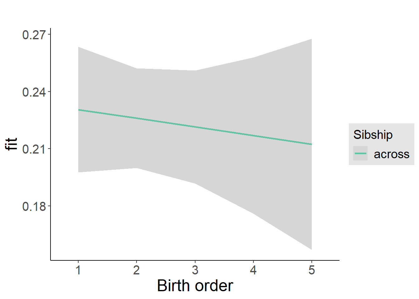
Add Birth Order Factor
Model Summary
m3_birthorder_nonlinear = update(m1_covariates_only, formula = . ~ . + birth_order_nonlinear)
tidy(m3_birthorder_nonlinear, conf.int = T, conf.level = 0.995)| effect | group | term | estimate | std.error | statistic | df | p.value | conf.low | conf.high |
|---|---|---|---|---|---|---|---|---|---|
| fixed | NA | (Intercept) | 0.4327 | 0.1243 | 3.482 | 4262 | 0.0005028 | 0.08386 | 0.7815 |
| fixed | NA | poly(age, 3, raw = TRUE)1 | -0.008547 | 0.01107 | -0.7719 | 4134 | 0.4402 | -0.03963 | 0.02253 |
| fixed | NA | poly(age, 3, raw = TRUE)2 | 0.00004687 | 0.0003067 | 0.1528 | 3982 | 0.8786 | -0.0008141 | 0.0009079 |
| fixed | NA | poly(age, 3, raw = TRUE)3 | 0.0000008012 | 0.000002674 | 0.2996 | 3852 | 0.7645 | -0.000006706 | 0.000008308 |
| fixed | NA | male | -0.0232 | 0.01256 | -1.848 | 4558 | 0.06469 | -0.05845 | 0.01204 |
| fixed | NA | sibling_count3 | 0.001244 | 0.01866 | 0.0667 | 3469 | 0.9468 | -0.05113 | 0.05362 |
| fixed | NA | sibling_count4 | 0.001444 | 0.01942 | 0.07434 | 3522 | 0.9407 | -0.05307 | 0.05595 |
| fixed | NA | sibling_count5 | 0.02355 | 0.02093 | 1.125 | 3580 | 0.2606 | -0.0352 | 0.08231 |
| fixed | NA | birth_order_nonlinear2 | 0.01144 | 0.01483 | 0.7719 | 3915 | 0.4402 | -0.03017 | 0.05306 |
| fixed | NA | birth_order_nonlinear3 | -0.02673 | 0.01879 | -1.423 | 3836 | 0.1548 | -0.07947 | 0.026 |
| fixed | NA | birth_order_nonlinear4 | 0.0003358 | 0.02453 | 0.01369 | 3759 | 0.9891 | -0.06853 | 0.0692 |
| fixed | NA | birth_order_nonlinear5 | -0.01665 | 0.03542 | -0.4701 | 3810 | 0.6383 | -0.1161 | 0.08278 |
| ran_pars | mother_pidlink | sd__(Intercept) | 0.155 | NA | NA | NA | NA | NA | NA |
| ran_pars | Residual | sd__Observation | 0.397 | NA | NA | NA | NA | NA | NA |
Coefficient Plot
plot_birthorder(m3_birthorder_nonlinear, separate = FALSE)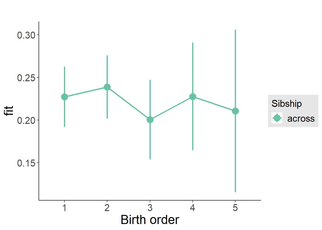
Add Interaction
Model Summary
m4_interaction = update(m3_birthorder_nonlinear, formula = . ~ . - birth_order_nonlinear - sibling_count + count_birth_order)
tidy(m4_interaction, conf.int = T, conf.level = 0.995)| effect | group | term | estimate | std.error | statistic | df | p.value | conf.low | conf.high |
|---|---|---|---|---|---|---|---|---|---|
| fixed | NA | (Intercept) | 0.4257 | 0.1245 | 3.42 | 4266 | 0.000631 | 0.07635 | 0.775 |
| fixed | NA | poly(age, 3, raw = TRUE)1 | -0.008696 | 0.01108 | -0.7846 | 4130 | 0.4328 | -0.03981 | 0.02242 |
| fixed | NA | poly(age, 3, raw = TRUE)2 | 0.00004825 | 0.0003069 | 0.1572 | 3978 | 0.8751 | -0.0008132 | 0.0009097 |
| fixed | NA | poly(age, 3, raw = TRUE)3 | 0.0000008123 | 0.000002675 | 0.3037 | 3847 | 0.7614 | -0.000006696 | 0.000008321 |
| fixed | NA | male | -0.0231 | 0.01256 | -1.839 | 4551 | 0.06604 | -0.05836 | 0.01217 |
| fixed | NA | count_birth_order2/2 | 0.03699 | 0.02523 | 1.466 | 3863 | 0.1427 | -0.03382 | 0.1078 |
| fixed | NA | count_birth_order1/3 | 0.02035 | 0.02439 | 0.8342 | 4611 | 0.4042 | -0.04812 | 0.08882 |
| fixed | NA | count_birth_order2/3 | 0.01117 | 0.02714 | 0.4117 | 4623 | 0.6806 | -0.06501 | 0.08735 |
| fixed | NA | count_birth_order3/3 | -0.01932 | 0.02984 | -0.6473 | 4625 | 0.5175 | -0.1031 | 0.06445 |
| fixed | NA | count_birth_order1/4 | 0.00998 | 0.02685 | 0.3716 | 4624 | 0.7102 | -0.0654 | 0.08536 |
| fixed | NA | count_birth_order2/4 | 0.02797 | 0.02881 | 0.9711 | 4625 | 0.3316 | -0.05289 | 0.1088 |
| fixed | NA | count_birth_order3/4 | -0.03503 | 0.03039 | -1.153 | 4624 | 0.2492 | -0.1203 | 0.05028 |
| fixed | NA | count_birth_order4/4 | 0.02918 | 0.03276 | 0.8906 | 4620 | 0.3732 | -0.06279 | 0.1211 |
| fixed | NA | count_birth_order1/5 | 0.04134 | 0.03027 | 1.366 | 4623 | 0.1721 | -0.04362 | 0.1263 |
| fixed | NA | count_birth_order2/5 | 0.02482 | 0.03216 | 0.772 | 4619 | 0.4402 | -0.06544 | 0.1151 |
| fixed | NA | count_birth_order3/5 | 0.03738 | 0.03382 | 1.105 | 4611 | 0.269 | -0.05755 | 0.1323 |
| fixed | NA | count_birth_order4/5 | 0.01092 | 0.03571 | 0.3059 | 4587 | 0.7597 | -0.08932 | 0.1112 |
| fixed | NA | count_birth_order5/5 | 0.01666 | 0.03582 | 0.4651 | 4606 | 0.6419 | -0.08389 | 0.1172 |
| ran_pars | mother_pidlink | sd__(Intercept) | 0.1545 | NA | NA | NA | NA | NA | NA |
| ran_pars | Residual | sd__Observation | 0.3972 | NA | NA | NA | NA | NA | NA |
Coefficient Plot
plot_birthorder(m4_interaction)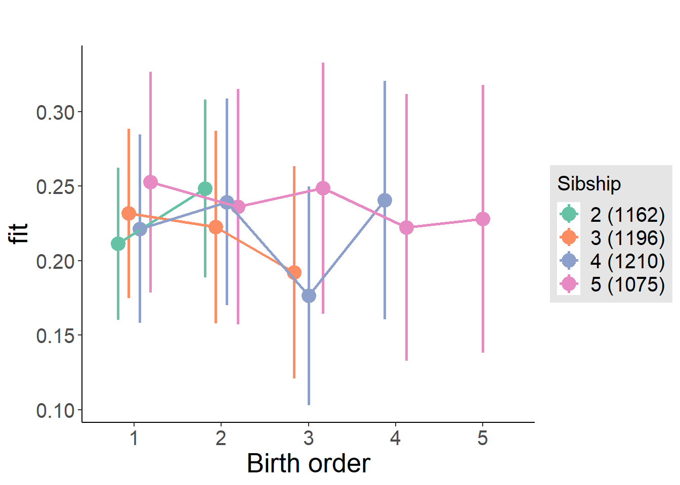
Model Comparison
###### Model 1 - Model 2
anova(m1_covariates_only, m2_birthorder_linear, m3_birthorder_nonlinear, m4_interaction)## refitting model(s) with ML (instead of REML)| Df | AIC | BIC | logLik | deviance | Chisq | Chi Df | Pr(>Chisq) |
|---|---|---|---|---|---|---|---|
| 10 | 5236 | 5301 | -2608 | 5216 | NA | NA | NA |
| 11 | 5238 | 5309 | -2608 | 5216 | 0.5488 | 1 | 0.4588 |
| 14 | 5240 | 5330 | -2606 | 5212 | 3.545 | 3 | 0.315 |
| 20 | 5247 | 5376 | -2604 | 5207 | 4.996 | 6 | 0.5444 |
Maternal birth order
outcome_uterus_m1 <- update(m2_birthorder_linear, data = birthorder %>%
mutate(sibling_count = sibling_count_uterus_alive_factor,
birth_order_nonlinear = birthorder_uterus_alive_factor,
birth_order = birthorder_uterus_alive,
count_birth_order = count_birthorder_uterus_alive) %>%
filter(sibling_count != "1"))
compare_models_markdown(outcome_uterus_m1)Basic Model
Model Summary
m1_covariates_only <- update(m2_birthorder_linear, formula = . ~ . - birth_order)
tidy(m1_covariates_only, conf.int = T, conf.level = 0.995)| effect | group | term | estimate | std.error | statistic | df | p.value | conf.low | conf.high |
|---|---|---|---|---|---|---|---|---|---|
| fixed | NA | (Intercept) | 0.4024 | 0.3641 | 1.105 | 2632 | 0.2692 | -0.6197 | 1.424 |
| fixed | NA | poly(age, 3, raw = TRUE)1 | -0.004128 | 0.0403 | -0.1025 | 2632 | 0.9184 | -0.1172 | 0.109 |
| fixed | NA | poly(age, 3, raw = TRUE)2 | -0.0001751 | 0.001427 | -0.1226 | 2632 | 0.9024 | -0.004182 | 0.003832 |
| fixed | NA | poly(age, 3, raw = TRUE)3 | 0.000003959 | 0.00001619 | 0.2445 | 2632 | 0.8069 | -0.0000415 | 0.00004942 |
| fixed | NA | male | -0.01904 | 0.01708 | -1.115 | 2612 | 0.265 | -0.06697 | 0.02889 |
| fixed | NA | sibling_count3 | 0.00216 | 0.02406 | 0.08977 | 2082 | 0.9285 | -0.06538 | 0.0697 |
| fixed | NA | sibling_count4 | 0.02206 | 0.02496 | 0.8839 | 1922 | 0.3769 | -0.04799 | 0.09211 |
| fixed | NA | sibling_count5 | 0.03022 | 0.0279 | 1.083 | 1690 | 0.2789 | -0.0481 | 0.1085 |
| ran_pars | mother_pidlink | sd__(Intercept) | 0.1583 | NA | NA | NA | NA | NA | NA |
| ran_pars | Residual | sd__Observation | 0.4044 | NA | NA | NA | NA | NA | NA |
Coefficient Plot
plot(allEffects(m1_covariates_only, confidence.level = 0.995))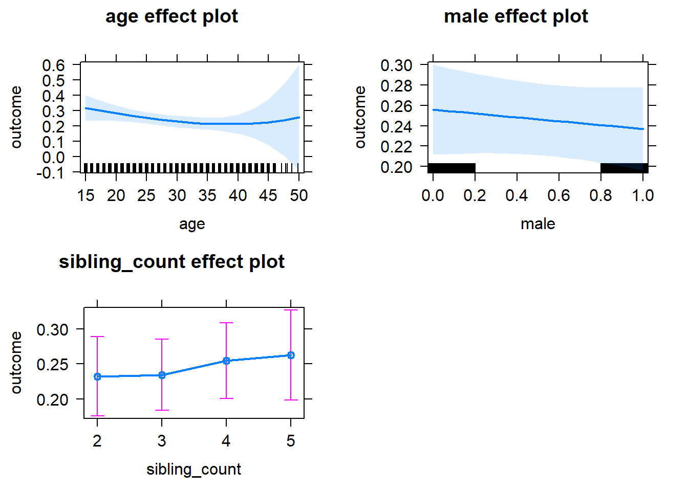
Add Birth Order Linear
Model Summary
tidy(m2_birthorder_linear, conf.int = T, conf.level = 0.995)| effect | group | term | estimate | std.error | statistic | df | p.value | conf.low | conf.high |
|---|---|---|---|---|---|---|---|---|---|
| fixed | NA | (Intercept) | 0.4019 | 0.3642 | 1.104 | 2631 | 0.2698 | -0.6203 | 1.424 |
| fixed | NA | birth_order | 0.004375 | 0.008576 | 0.5101 | 2453 | 0.61 | -0.0197 | 0.02845 |
| fixed | NA | poly(age, 3, raw = TRUE)1 | -0.004594 | 0.04031 | -0.114 | 2631 | 0.9093 | -0.1178 | 0.1086 |
| fixed | NA | poly(age, 3, raw = TRUE)2 | -0.0001661 | 0.001428 | -0.1163 | 2631 | 0.9074 | -0.004174 | 0.003842 |
| fixed | NA | poly(age, 3, raw = TRUE)3 | 0.000003975 | 0.0000162 | 0.2454 | 2631 | 0.8061 | -0.00004149 | 0.00004944 |
| fixed | NA | male | -0.01903 | 0.01708 | -1.114 | 2611 | 0.2652 | -0.06697 | 0.02891 |
| fixed | NA | sibling_count3 | 0.00009149 | 0.02441 | 0.003749 | 2114 | 0.997 | -0.06842 | 0.0686 |
| fixed | NA | sibling_count4 | 0.01755 | 0.02647 | 0.6629 | 2045 | 0.5075 | -0.05676 | 0.09186 |
| fixed | NA | sibling_count5 | 0.02273 | 0.03154 | 0.7207 | 2003 | 0.4711 | -0.0658 | 0.1113 |
| ran_pars | mother_pidlink | sd__(Intercept) | 0.1587 | NA | NA | NA | NA | NA | NA |
| ran_pars | Residual | sd__Observation | 0.4043 | NA | NA | NA | NA | NA | NA |
Coefficient Plot
plot_birthorder2(m2_birthorder_linear, separate = FALSE)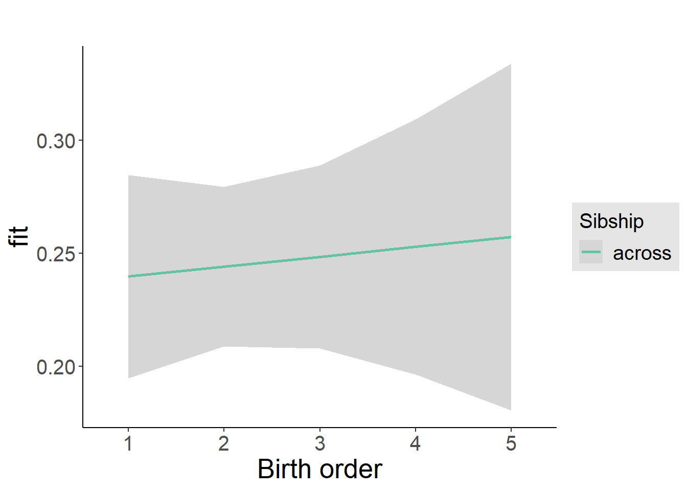
Add Birth Order Factor
Model Summary
m3_birthorder_nonlinear = update(m1_covariates_only, formula = . ~ . + birth_order_nonlinear)
tidy(m3_birthorder_nonlinear, conf.int = T, conf.level = 0.995)| effect | group | term | estimate | std.error | statistic | df | p.value | conf.low | conf.high |
|---|---|---|---|---|---|---|---|---|---|
| fixed | NA | (Intercept) | 0.4162 | 0.3649 | 1.141 | 2627 | 0.2542 | -0.6081 | 1.441 |
| fixed | NA | poly(age, 3, raw = TRUE)1 | -0.006038 | 0.04037 | -0.1496 | 2628 | 0.8811 | -0.1194 | 0.1073 |
| fixed | NA | poly(age, 3, raw = TRUE)2 | -0.0001192 | 0.00143 | -0.08336 | 2628 | 0.9336 | -0.004133 | 0.003895 |
| fixed | NA | poly(age, 3, raw = TRUE)3 | 0.000003505 | 0.00001622 | 0.2161 | 2628 | 0.8289 | -0.00004202 | 0.00004903 |
| fixed | NA | male | -0.01979 | 0.01709 | -1.158 | 2609 | 0.247 | -0.06776 | 0.02818 |
| fixed | NA | sibling_count3 | 0.003015 | 0.02475 | 0.1218 | 2170 | 0.9031 | -0.06647 | 0.0725 |
| fixed | NA | sibling_count4 | 0.01462 | 0.02681 | 0.5451 | 2097 | 0.5858 | -0.06065 | 0.08988 |
| fixed | NA | sibling_count5 | 0.02757 | 0.03192 | 0.8637 | 2046 | 0.3878 | -0.06203 | 0.1172 |
| fixed | NA | birth_order_nonlinear2 | 0.01772 | 0.02042 | 0.8681 | 2234 | 0.3854 | -0.03959 | 0.07504 |
| fixed | NA | birth_order_nonlinear3 | -0.003046 | 0.02491 | -0.1223 | 2270 | 0.9027 | -0.07296 | 0.06687 |
| fixed | NA | birth_order_nonlinear4 | 0.0467 | 0.0332 | 1.407 | 2332 | 0.1596 | -0.04649 | 0.1399 |
| fixed | NA | birth_order_nonlinear5 | -0.02429 | 0.05138 | -0.4727 | 2250 | 0.6365 | -0.1685 | 0.1199 |
| ran_pars | mother_pidlink | sd__(Intercept) | 0.1593 | NA | NA | NA | NA | NA | NA |
| ran_pars | Residual | sd__Observation | 0.4041 | NA | NA | NA | NA | NA | NA |
Coefficient Plot
plot_birthorder(m3_birthorder_nonlinear, separate = FALSE)
Add Interaction
Model Summary
m4_interaction = update(m3_birthorder_nonlinear, formula = . ~ . - birth_order_nonlinear - sibling_count + count_birth_order)
tidy(m4_interaction, conf.int = T, conf.level = 0.995)| effect | group | term | estimate | std.error | statistic | df | p.value | conf.low | conf.high |
|---|---|---|---|---|---|---|---|---|---|
| fixed | NA | (Intercept) | 0.4303 | 0.3652 | 1.178 | 2621 | 0.2388 | -0.5947 | 1.455 |
| fixed | NA | poly(age, 3, raw = TRUE)1 | -0.006869 | 0.0404 | -0.17 | 2622 | 0.865 | -0.1203 | 0.1065 |
| fixed | NA | poly(age, 3, raw = TRUE)2 | -0.0001017 | 0.001431 | -0.07106 | 2622 | 0.9434 | -0.004119 | 0.003915 |
| fixed | NA | poly(age, 3, raw = TRUE)3 | 0.000003435 | 0.00001623 | 0.2116 | 2622 | 0.8324 | -0.00004213 | 0.000049 |
| fixed | NA | male | -0.01933 | 0.01711 | -1.13 | 2601 | 0.2586 | -0.06736 | 0.02869 |
| fixed | NA | count_birth_order2/2 | 0.005388 | 0.03721 | 0.1448 | 2256 | 0.8849 | -0.09907 | 0.1098 |
| fixed | NA | count_birth_order1/3 | 0.0145 | 0.03143 | 0.4612 | 2620 | 0.6447 | -0.07372 | 0.1027 |
| fixed | NA | count_birth_order2/3 | 0.009415 | 0.0349 | 0.2698 | 2624 | 0.7874 | -0.08855 | 0.1074 |
| fixed | NA | count_birth_order3/3 | -0.02462 | 0.03799 | -0.6481 | 2619 | 0.517 | -0.1313 | 0.08202 |
| fixed | NA | count_birth_order1/4 | -0.01828 | 0.03614 | -0.5058 | 2624 | 0.613 | -0.1197 | 0.08317 |
| fixed | NA | count_birth_order2/4 | 0.02588 | 0.03822 | 0.6772 | 2621 | 0.4984 | -0.0814 | 0.1332 |
| fixed | NA | count_birth_order3/4 | 0.05347 | 0.03961 | 1.35 | 2614 | 0.1771 | -0.05771 | 0.1646 |
| fixed | NA | count_birth_order4/4 | 0.05344 | 0.04234 | 1.262 | 2611 | 0.207 | -0.06541 | 0.1723 |
| fixed | NA | count_birth_order1/5 | 0.01748 | 0.04768 | 0.3665 | 2622 | 0.714 | -0.1164 | 0.1513 |
| fixed | NA | count_birth_order2/5 | 0.08537 | 0.05123 | 1.666 | 2602 | 0.09577 | -0.05844 | 0.2292 |
| fixed | NA | count_birth_order3/5 | -0.01865 | 0.04865 | -0.3834 | 2601 | 0.7015 | -0.1552 | 0.1179 |
| fixed | NA | count_birth_order4/5 | 0.07684 | 0.0474 | 1.621 | 2596 | 0.1051 | -0.05622 | 0.2099 |
| fixed | NA | count_birth_order5/5 | -0.0006437 | 0.04985 | -0.01291 | 2588 | 0.9897 | -0.1406 | 0.1393 |
| ran_pars | mother_pidlink | sd__(Intercept) | 0.1606 | NA | NA | NA | NA | NA | NA |
| ran_pars | Residual | sd__Observation | 0.4036 | NA | NA | NA | NA | NA | NA |
Coefficient Plot
plot_birthorder(m4_interaction)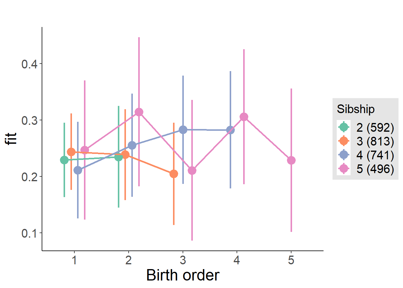
Model Comparison
###### Model 1 - Model 2
anova(m1_covariates_only, m2_birthorder_linear, m3_birthorder_nonlinear, m4_interaction)## refitting model(s) with ML (instead of REML)| Df | AIC | BIC | logLik | deviance | Chisq | Chi Df | Pr(>Chisq) |
|---|---|---|---|---|---|---|---|
| 10 | 3088 | 3147 | -1534 | 3068 | NA | NA | NA |
| 11 | 3090 | 3154 | -1534 | 3068 | 0.2587 | 1 | 0.611 |
| 14 | 3093 | 3175 | -1532 | 3065 | 3.273 | 3 | 0.3515 |
| 20 | 3098 | 3216 | -1529 | 3058 | 6.141 | 6 | 0.4076 |
Maternal pregnancy order
outcome_preg_m1 <- update(m2_birthorder_linear, data = birthorder %>%
mutate(sibling_count = sibling_count_uterus_preg_factor,
birth_order_nonlinear = birthorder_uterus_preg_factor,
birth_order = birthorder_uterus_preg,
count_birth_order = count_birthorder_uterus_preg
) %>%
filter(sibling_count != "1"))
compare_models_markdown(outcome_preg_m1)Basic Model
Model Summary
m1_covariates_only <- update(m2_birthorder_linear, formula = . ~ . - birth_order)
tidy(m1_covariates_only, conf.int = T, conf.level = 0.995)| effect | group | term | estimate | std.error | statistic | df | p.value | conf.low | conf.high |
|---|---|---|---|---|---|---|---|---|---|
| fixed | NA | (Intercept) | 0.4734 | 0.3758 | 1.26 | 2418 | 0.2079 | -0.5816 | 1.528 |
| fixed | NA | poly(age, 3, raw = TRUE)1 | -0.01121 | 0.04162 | -0.2694 | 2419 | 0.7876 | -0.128 | 0.1056 |
| fixed | NA | poly(age, 3, raw = TRUE)2 | 0.00001013 | 0.001474 | 0.006874 | 2419 | 0.9945 | -0.004129 | 0.004149 |
| fixed | NA | poly(age, 3, raw = TRUE)3 | 0.000002715 | 0.00001673 | 0.1623 | 2418 | 0.8711 | -0.00004425 | 0.00004968 |
| fixed | NA | male | -0.02601 | 0.01776 | -1.465 | 2397 | 0.1432 | -0.07587 | 0.02384 |
| fixed | NA | sibling_count3 | 0.02154 | 0.02633 | 0.8181 | 1943 | 0.4134 | -0.05237 | 0.09545 |
| fixed | NA | sibling_count4 | 0.01969 | 0.02669 | 0.7376 | 1847 | 0.4608 | -0.05523 | 0.0946 |
| fixed | NA | sibling_count5 | 0.03169 | 0.0282 | 1.124 | 1713 | 0.2613 | -0.04747 | 0.1108 |
| ran_pars | mother_pidlink | sd__(Intercept) | 0.1625 | NA | NA | NA | NA | NA | NA |
| ran_pars | Residual | sd__Observation | 0.4013 | NA | NA | NA | NA | NA | NA |
Coefficient Plot
plot(allEffects(m1_covariates_only, confidence.level = 0.995))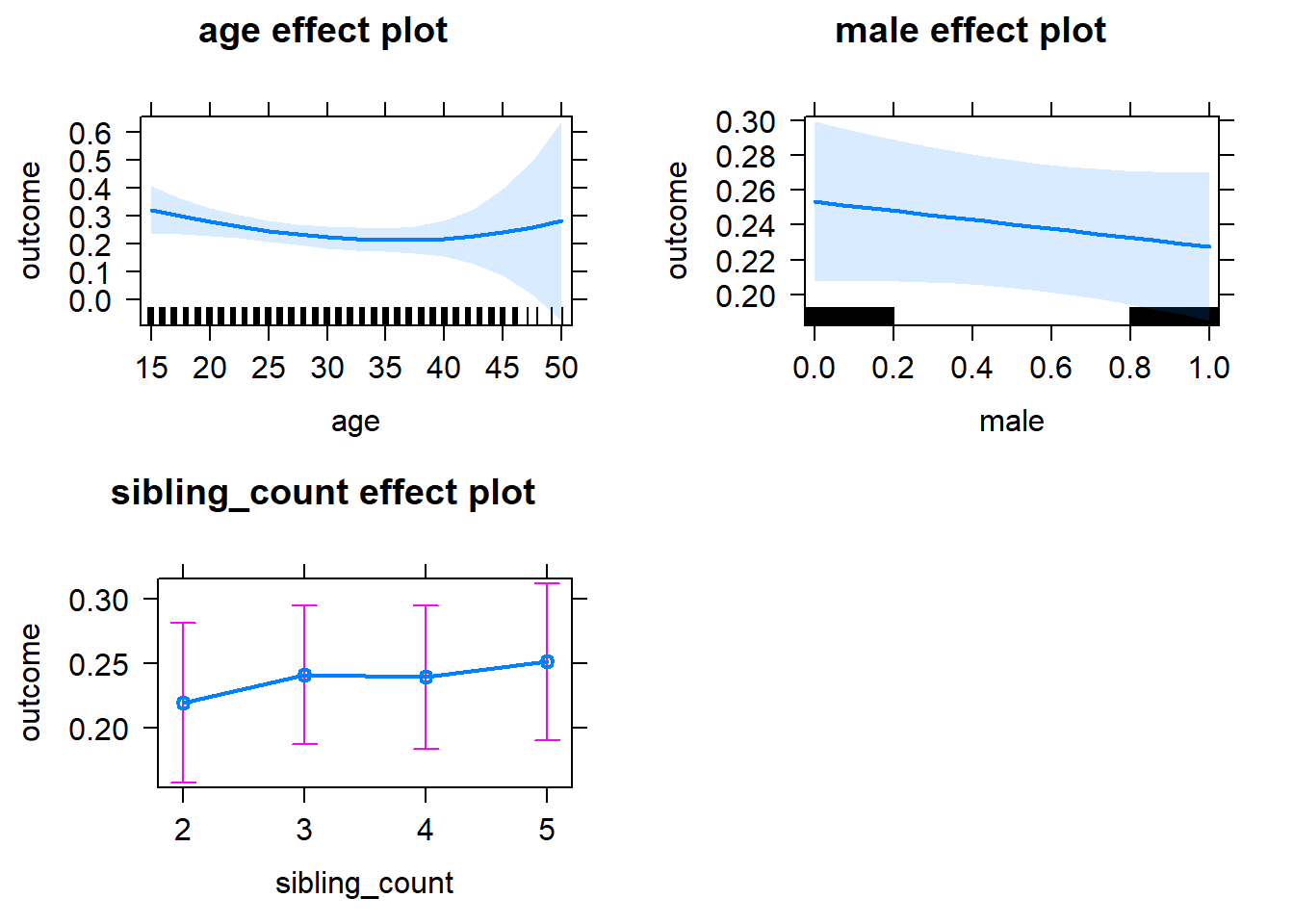
Add Birth Order Linear
Model Summary
tidy(m2_birthorder_linear, conf.int = T, conf.level = 0.995)| effect | group | term | estimate | std.error | statistic | df | p.value | conf.low | conf.high |
|---|---|---|---|---|---|---|---|---|---|
| fixed | NA | (Intercept) | 0.4726 | 0.376 | 1.257 | 2417 | 0.2089 | -0.5827 | 1.528 |
| fixed | NA | birth_order | 0.00139 | 0.008678 | 0.1602 | 2304 | 0.8727 | -0.02297 | 0.02575 |
| fixed | NA | poly(age, 3, raw = TRUE)1 | -0.01131 | 0.04163 | -0.2716 | 2418 | 0.7859 | -0.1282 | 0.1056 |
| fixed | NA | poly(age, 3, raw = TRUE)2 | 0.00001177 | 0.001475 | 0.007984 | 2418 | 0.9936 | -0.004128 | 0.004151 |
| fixed | NA | poly(age, 3, raw = TRUE)3 | 0.000002729 | 0.00001673 | 0.1631 | 2417 | 0.8705 | -0.00004424 | 0.0000497 |
| fixed | NA | male | -0.02598 | 0.01777 | -1.462 | 2396 | 0.1438 | -0.07584 | 0.02389 |
| fixed | NA | sibling_count3 | 0.02088 | 0.02666 | 0.783 | 1961 | 0.4337 | -0.05396 | 0.09572 |
| fixed | NA | sibling_count4 | 0.01837 | 0.02793 | 0.6576 | 1919 | 0.5109 | -0.06004 | 0.09677 |
| fixed | NA | sibling_count5 | 0.02946 | 0.03145 | 0.9368 | 1929 | 0.349 | -0.05881 | 0.1177 |
| ran_pars | mother_pidlink | sd__(Intercept) | 0.1626 | NA | NA | NA | NA | NA | NA |
| ran_pars | Residual | sd__Observation | 0.4014 | NA | NA | NA | NA | NA | NA |
Coefficient Plot
plot_birthorder2(m2_birthorder_linear, separate = FALSE)
Add Birth Order Factor
Model Summary
m3_birthorder_nonlinear = update(m1_covariates_only, formula = . ~ . + birth_order_nonlinear)
tidy(m3_birthorder_nonlinear, conf.int = T, conf.level = 0.995)| effect | group | term | estimate | std.error | statistic | df | p.value | conf.low | conf.high |
|---|---|---|---|---|---|---|---|---|---|
| fixed | NA | (Intercept) | 0.4823 | 0.3769 | 1.28 | 2414 | 0.2008 | -0.5756 | 1.54 |
| fixed | NA | poly(age, 3, raw = TRUE)1 | -0.01246 | 0.04172 | -0.2987 | 2414 | 0.7652 | -0.1296 | 0.1047 |
| fixed | NA | poly(age, 3, raw = TRUE)2 | 0.00005189 | 0.001478 | 0.03511 | 2414 | 0.972 | -0.004097 | 0.0042 |
| fixed | NA | poly(age, 3, raw = TRUE)3 | 0.000002313 | 0.00001677 | 0.138 | 2414 | 0.8903 | -0.00004475 | 0.00004938 |
| fixed | NA | male | -0.027 | 0.01777 | -1.519 | 2392 | 0.1289 | -0.07688 | 0.02289 |
| fixed | NA | sibling_count3 | 0.0236 | 0.02702 | 0.8736 | 2004 | 0.3824 | -0.05224 | 0.09945 |
| fixed | NA | sibling_count4 | 0.01345 | 0.02826 | 0.476 | 1959 | 0.6341 | -0.06589 | 0.09279 |
| fixed | NA | sibling_count5 | 0.03285 | 0.03164 | 1.038 | 1950 | 0.2993 | -0.05596 | 0.1217 |
| fixed | NA | birth_order_nonlinear2 | 0.008117 | 0.02107 | 0.3852 | 2050 | 0.7001 | -0.05104 | 0.06727 |
| fixed | NA | birth_order_nonlinear3 | -0.009046 | 0.026 | -0.3479 | 2126 | 0.7279 | -0.08203 | 0.06394 |
| fixed | NA | birth_order_nonlinear4 | 0.04929 | 0.03435 | 1.435 | 2185 | 0.1515 | -0.04715 | 0.1457 |
| fixed | NA | birth_order_nonlinear5 | -0.04467 | 0.04924 | -0.9073 | 2091 | 0.3644 | -0.1829 | 0.09355 |
| ran_pars | mother_pidlink | sd__(Intercept) | 0.1642 | NA | NA | NA | NA | NA | NA |
| ran_pars | Residual | sd__Observation | 0.4006 | NA | NA | NA | NA | NA | NA |
Coefficient Plot
plot_birthorder(m3_birthorder_nonlinear, separate = FALSE)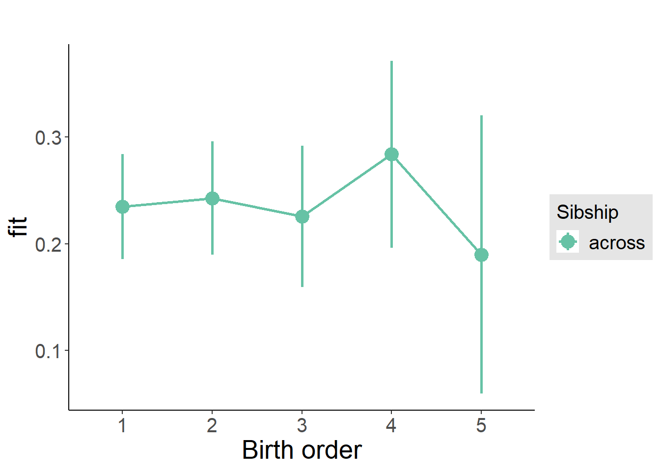
Add Interaction
Model Summary
m4_interaction = update(m3_birthorder_nonlinear, formula = . ~ . - birth_order_nonlinear - sibling_count + count_birth_order)
tidy(m4_interaction, conf.int = T, conf.level = 0.995)| effect | group | term | estimate | std.error | statistic | df | p.value | conf.low | conf.high |
|---|---|---|---|---|---|---|---|---|---|
| fixed | NA | (Intercept) | 0.4692 | 0.3776 | 1.243 | 2408 | 0.2141 | -0.5907 | 1.529 |
| fixed | NA | poly(age, 3, raw = TRUE)1 | -0.01088 | 0.0418 | -0.2602 | 2408 | 0.7948 | -0.1282 | 0.1065 |
| fixed | NA | poly(age, 3, raw = TRUE)2 | -0.00001648 | 0.001481 | -0.01113 | 2408 | 0.9911 | -0.004173 | 0.00414 |
| fixed | NA | poly(age, 3, raw = TRUE)3 | 0.000003221 | 0.0000168 | 0.1917 | 2408 | 0.848 | -0.00004394 | 0.00005038 |
| fixed | NA | male | -0.02625 | 0.01782 | -1.473 | 2384 | 0.1408 | -0.07627 | 0.02377 |
| fixed | NA | count_birth_order2/2 | 0.01227 | 0.04069 | 0.3015 | 2125 | 0.7631 | -0.1019 | 0.1265 |
| fixed | NA | count_birth_order1/3 | 0.04134 | 0.03469 | 1.192 | 2405 | 0.2335 | -0.05603 | 0.1387 |
| fixed | NA | count_birth_order2/3 | 0.03165 | 0.03771 | 0.8393 | 2409 | 0.4014 | -0.07421 | 0.1375 |
| fixed | NA | count_birth_order3/3 | -0.0141 | 0.04176 | -0.3375 | 2403 | 0.7358 | -0.1313 | 0.1031 |
| fixed | NA | count_birth_order1/4 | 0.008425 | 0.03775 | 0.2232 | 2408 | 0.8234 | -0.09754 | 0.1144 |
| fixed | NA | count_birth_order2/4 | 0.00617 | 0.03968 | 0.1555 | 2408 | 0.8764 | -0.1052 | 0.1175 |
| fixed | NA | count_birth_order3/4 | 0.03581 | 0.04289 | 0.835 | 2399 | 0.4038 | -0.08457 | 0.1562 |
| fixed | NA | count_birth_order4/4 | 0.06662 | 0.04651 | 1.432 | 2392 | 0.1522 | -0.06393 | 0.1972 |
| fixed | NA | count_birth_order1/5 | 0.009166 | 0.04567 | 0.2007 | 2408 | 0.841 | -0.119 | 0.1374 |
| fixed | NA | count_birth_order2/5 | 0.06819 | 0.0467 | 1.46 | 2402 | 0.1444 | -0.06292 | 0.1993 |
| fixed | NA | count_birth_order3/5 | 0.02842 | 0.04796 | 0.5925 | 2389 | 0.5536 | -0.1062 | 0.1631 |
| fixed | NA | count_birth_order4/5 | 0.08194 | 0.04871 | 1.682 | 2380 | 0.09263 | -0.05478 | 0.2187 |
| fixed | NA | count_birth_order5/5 | -0.01018 | 0.04943 | -0.2059 | 2373 | 0.8369 | -0.1489 | 0.1286 |
| ran_pars | mother_pidlink | sd__(Intercept) | 0.1654 | NA | NA | NA | NA | NA | NA |
| ran_pars | Residual | sd__Observation | 0.4005 | NA | NA | NA | NA | NA | NA |
Coefficient Plot
plot_birthorder(m4_interaction)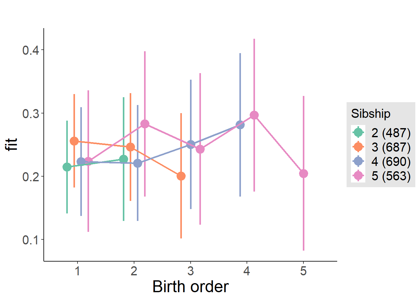
Model Comparison
###### Model 1 - Model 2
anova(m1_covariates_only, m2_birthorder_linear, m3_birthorder_nonlinear, m4_interaction)## refitting model(s) with ML (instead of REML)| Df | AIC | BIC | logLik | deviance | Chisq | Chi Df | Pr(>Chisq) |
|---|---|---|---|---|---|---|---|
| 10 | 2822 | 2880 | -1401 | 2802 | NA | NA | NA |
| 11 | 2824 | 2888 | -1401 | 2802 | 0.0254 | 1 | 0.8734 |
| 14 | 2826 | 2907 | -1399 | 2798 | 4.247 | 3 | 0.236 |
| 20 | 2835 | 2950 | -1397 | 2795 | 3.294 | 6 | 0.7711 |
Parental full sibling order
outcome_parental_m1 <- update(m2_birthorder_linear, data = birthorder %>%
mutate(sibling_count = sibling_count_genes_factor,
birth_order_nonlinear = birthorder_genes_factor,
birth_order = birthorder_genes,
count_birth_order = count_birthorder_genes
) %>%
filter(sibling_count != "1"))
compare_models_markdown(outcome_parental_m1)Basic Model
Model Summary
m1_covariates_only <- update(m2_birthorder_linear, formula = . ~ . - birth_order)
tidy(m1_covariates_only, conf.int = T, conf.level = 0.995)| effect | group | term | estimate | std.error | statistic | df | p.value | conf.low | conf.high |
|---|---|---|---|---|---|---|---|---|---|
| fixed | NA | (Intercept) | 0.4815 | 0.3681 | 1.308 | 2634 | 0.191 | -0.5518 | 1.515 |
| fixed | NA | poly(age, 3, raw = TRUE)1 | -0.01328 | 0.04085 | -0.3251 | 2635 | 0.7451 | -0.128 | 0.1014 |
| fixed | NA | poly(age, 3, raw = TRUE)2 | 0.0001476 | 0.00145 | 0.1018 | 2635 | 0.919 | -0.003924 | 0.004219 |
| fixed | NA | poly(age, 3, raw = TRUE)3 | 0.0000005726 | 0.0000165 | 0.03471 | 2634 | 0.9723 | -0.00004574 | 0.00004689 |
| fixed | NA | male | -0.02288 | 0.01708 | -1.339 | 2617 | 0.1805 | -0.07083 | 0.02507 |
| fixed | NA | sibling_count3 | 0.007384 | 0.02357 | 0.3133 | 2091 | 0.7541 | -0.05878 | 0.07355 |
| fixed | NA | sibling_count4 | 0.01739 | 0.02478 | 0.7018 | 1932 | 0.4829 | -0.05217 | 0.08694 |
| fixed | NA | sibling_count5 | 0.03453 | 0.02851 | 1.211 | 1622 | 0.226 | -0.0455 | 0.1146 |
| ran_pars | mother_pidlink | sd__(Intercept) | 0.1567 | NA | NA | NA | NA | NA | NA |
| ran_pars | Residual | sd__Observation | 0.4054 | NA | NA | NA | NA | NA | NA |
Coefficient Plot
plot(allEffects(m1_covariates_only, confidence.level = 0.995))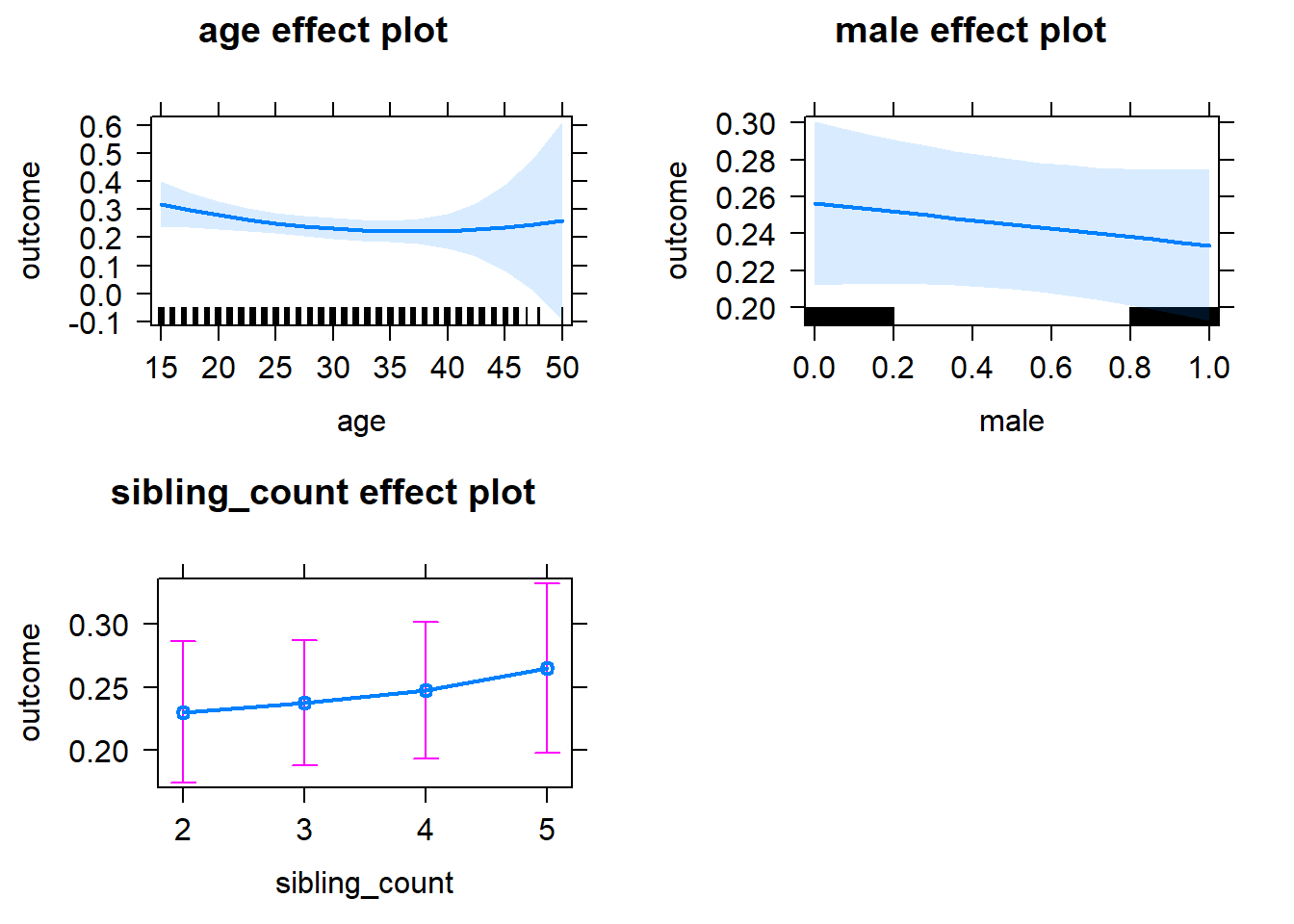
Add Birth Order Linear
Model Summary
tidy(m2_birthorder_linear, conf.int = T, conf.level = 0.995)| effect | group | term | estimate | std.error | statistic | df | p.value | conf.low | conf.high |
|---|---|---|---|---|---|---|---|---|---|
| fixed | NA | (Intercept) | 0.4807 | 0.3681 | 1.306 | 2633 | 0.1917 | -0.5526 | 1.514 |
| fixed | NA | birth_order | 0.006053 | 0.008688 | 0.6967 | 2442 | 0.4861 | -0.01833 | 0.03044 |
| fixed | NA | poly(age, 3, raw = TRUE)1 | -0.01394 | 0.04087 | -0.341 | 2633 | 0.7331 | -0.1287 | 0.1008 |
| fixed | NA | poly(age, 3, raw = TRUE)2 | 0.000161 | 0.001451 | 0.1109 | 2633 | 0.9117 | -0.003911 | 0.004233 |
| fixed | NA | poly(age, 3, raw = TRUE)3 | 0.0000005789 | 0.0000165 | 0.03509 | 2633 | 0.972 | -0.00004574 | 0.0000469 |
| fixed | NA | male | -0.0228 | 0.01708 | -1.334 | 2616 | 0.1822 | -0.07075 | 0.02516 |
| fixed | NA | sibling_count3 | 0.004481 | 0.02394 | 0.1871 | 2122 | 0.8516 | -0.06273 | 0.07169 |
| fixed | NA | sibling_count4 | 0.01121 | 0.02632 | 0.4261 | 2064 | 0.67 | -0.06265 | 0.08508 |
| fixed | NA | sibling_count5 | 0.02457 | 0.03191 | 0.7698 | 1912 | 0.4415 | -0.06501 | 0.1141 |
| ran_pars | mother_pidlink | sd__(Intercept) | 0.1572 | NA | NA | NA | NA | NA | NA |
| ran_pars | Residual | sd__Observation | 0.4053 | NA | NA | NA | NA | NA | NA |
Coefficient Plot
plot_birthorder2(m2_birthorder_linear, separate = FALSE)
Add Birth Order Factor
Model Summary
m3_birthorder_nonlinear = update(m1_covariates_only, formula = . ~ . + birth_order_nonlinear)
tidy(m3_birthorder_nonlinear, conf.int = T, conf.level = 0.995)| effect | group | term | estimate | std.error | statistic | df | p.value | conf.low | conf.high |
|---|---|---|---|---|---|---|---|---|---|
| fixed | NA | (Intercept) | 0.4948 | 0.3689 | 1.341 | 2629 | 0.18 | -0.5407 | 1.53 |
| fixed | NA | poly(age, 3, raw = TRUE)1 | -0.01525 | 0.04093 | -0.3727 | 2630 | 0.7094 | -0.1302 | 0.09965 |
| fixed | NA | poly(age, 3, raw = TRUE)2 | 0.0002064 | 0.001453 | 0.142 | 2630 | 0.8871 | -0.003873 | 0.004285 |
| fixed | NA | poly(age, 3, raw = TRUE)3 | 0.00000008827 | 0.00001653 | 0.005341 | 2630 | 0.9957 | -0.0000463 | 0.00004648 |
| fixed | NA | male | -0.0234 | 0.0171 | -1.368 | 2614 | 0.1713 | -0.0714 | 0.0246 |
| fixed | NA | sibling_count3 | 0.007534 | 0.02431 | 0.3099 | 2180 | 0.7566 | -0.0607 | 0.07577 |
| fixed | NA | sibling_count4 | 0.01047 | 0.02666 | 0.3928 | 2116 | 0.6945 | -0.06436 | 0.0853 |
| fixed | NA | sibling_count5 | 0.02813 | 0.03242 | 0.8678 | 1967 | 0.3856 | -0.06286 | 0.1191 |
| fixed | NA | birth_order_nonlinear2 | 0.01926 | 0.02023 | 0.952 | 2229 | 0.3412 | -0.03753 | 0.07604 |
| fixed | NA | birth_order_nonlinear3 | 0.0006313 | 0.02488 | 0.02538 | 2277 | 0.9798 | -0.0692 | 0.07046 |
| fixed | NA | birth_order_nonlinear4 | 0.04094 | 0.03411 | 1.2 | 2325 | 0.2302 | -0.05482 | 0.1367 |
| fixed | NA | birth_order_nonlinear5 | 0.0005619 | 0.0545 | 0.01031 | 2265 | 0.9918 | -0.1524 | 0.1535 |
| ran_pars | mother_pidlink | sd__(Intercept) | 0.157 | NA | NA | NA | NA | NA | NA |
| ran_pars | Residual | sd__Observation | 0.4055 | NA | NA | NA | NA | NA | NA |
Coefficient Plot
plot_birthorder(m3_birthorder_nonlinear, separate = FALSE)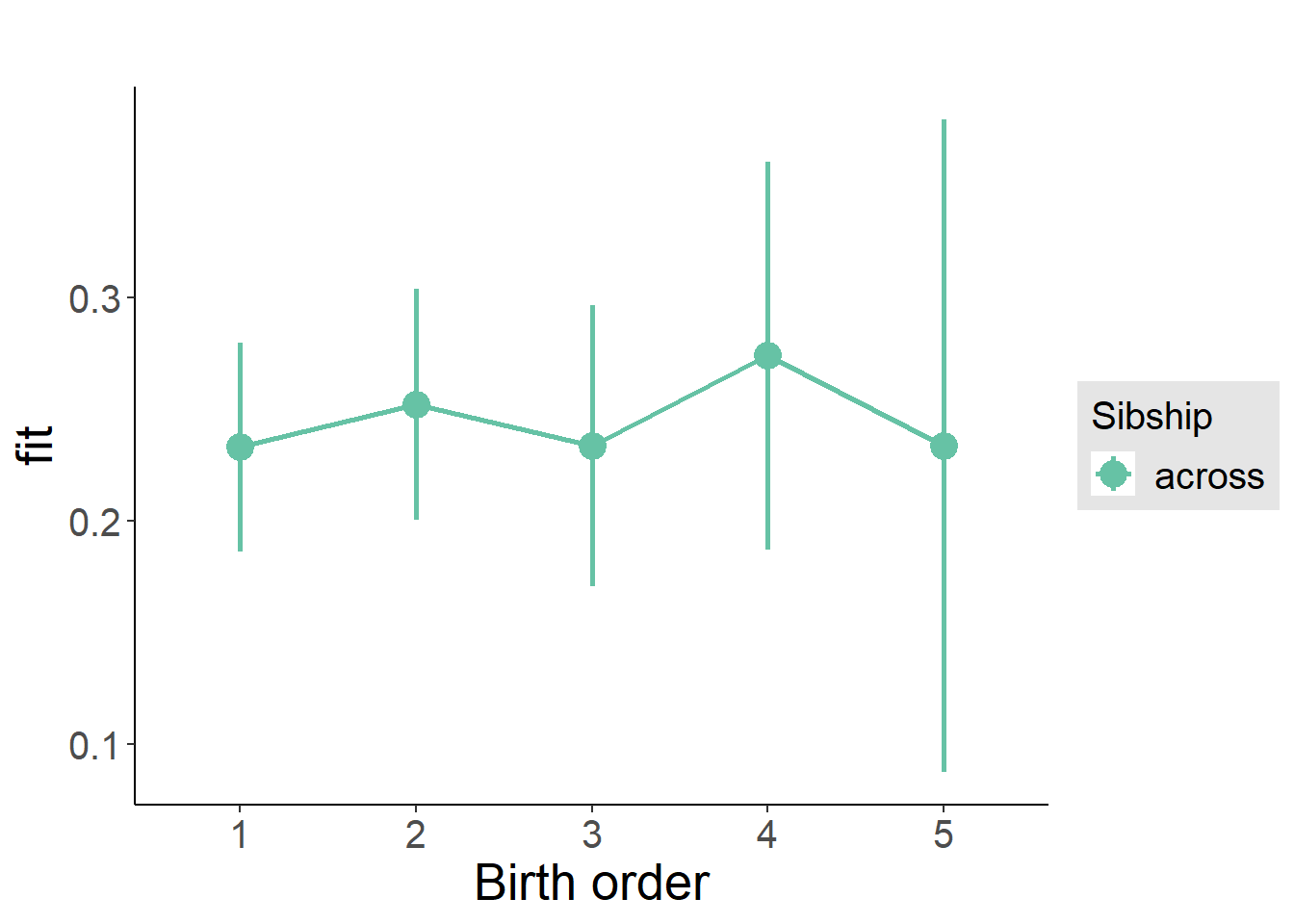
Add Interaction
Model Summary
m4_interaction = update(m3_birthorder_nonlinear, formula = . ~ . - birth_order_nonlinear - sibling_count + count_birth_order)
tidy(m4_interaction, conf.int = T, conf.level = 0.995)| effect | group | term | estimate | std.error | statistic | df | p.value | conf.low | conf.high |
|---|---|---|---|---|---|---|---|---|---|
| fixed | NA | (Intercept) | 0.5024 | 0.3693 | 1.36 | 2623 | 0.1739 | -0.5344 | 1.539 |
| fixed | NA | poly(age, 3, raw = TRUE)1 | -0.01596 | 0.04099 | -0.3894 | 2624 | 0.697 | -0.131 | 0.09909 |
| fixed | NA | poly(age, 3, raw = TRUE)2 | 0.000227 | 0.001455 | 0.156 | 2624 | 0.876 | -0.003858 | 0.004312 |
| fixed | NA | poly(age, 3, raw = TRUE)3 | -0.00000009427 | 0.00001655 | -0.005695 | 2624 | 0.9955 | -0.00004656 | 0.00004637 |
| fixed | NA | male | -0.02334 | 0.01713 | -1.363 | 2607 | 0.1731 | -0.07141 | 0.02473 |
| fixed | NA | count_birth_order2/2 | 0.01831 | 0.03626 | 0.505 | 2253 | 0.6136 | -0.08348 | 0.1201 |
| fixed | NA | count_birth_order1/3 | 0.01864 | 0.03093 | 0.6026 | 2624 | 0.5468 | -0.06819 | 0.1055 |
| fixed | NA | count_birth_order2/3 | 0.02321 | 0.03436 | 0.6754 | 2628 | 0.4995 | -0.07325 | 0.1197 |
| fixed | NA | count_birth_order3/3 | -0.009623 | 0.03699 | -0.2602 | 2622 | 0.7947 | -0.1134 | 0.0942 |
| fixed | NA | count_birth_order1/4 | -0.01195 | 0.03637 | -0.3286 | 2628 | 0.7425 | -0.1141 | 0.09015 |
| fixed | NA | count_birth_order2/4 | 0.02546 | 0.03812 | 0.6679 | 2624 | 0.5043 | -0.08155 | 0.1325 |
| fixed | NA | count_birth_order3/4 | 0.04243 | 0.03954 | 1.073 | 2617 | 0.2833 | -0.06856 | 0.1534 |
| fixed | NA | count_birth_order4/4 | 0.05387 | 0.04291 | 1.255 | 2613 | 0.2094 | -0.06657 | 0.1743 |
| fixed | NA | count_birth_order1/5 | 0.0315 | 0.04767 | 0.6608 | 2627 | 0.5088 | -0.1023 | 0.1653 |
| fixed | NA | count_birth_order2/5 | 0.06755 | 0.05301 | 1.274 | 2601 | 0.2027 | -0.08125 | 0.2164 |
| fixed | NA | count_birth_order3/5 | 0.007274 | 0.0516 | 0.141 | 2597 | 0.8879 | -0.1376 | 0.1521 |
| fixed | NA | count_birth_order4/5 | 0.0658 | 0.04963 | 1.326 | 2598 | 0.185 | -0.07351 | 0.2051 |
| fixed | NA | count_birth_order5/5 | 0.02832 | 0.05268 | 0.5375 | 2591 | 0.591 | -0.1196 | 0.1762 |
| ran_pars | mother_pidlink | sd__(Intercept) | 0.1581 | NA | NA | NA | NA | NA | NA |
| ran_pars | Residual | sd__Observation | 0.4054 | NA | NA | NA | NA | NA | NA |
Coefficient Plot
plot_birthorder(m4_interaction)
Model Comparison
###### Model 1 - Model 2
anova(m1_covariates_only, m2_birthorder_linear, m3_birthorder_nonlinear, m4_interaction)## refitting model(s) with ML (instead of REML)| Df | AIC | BIC | logLik | deviance | Chisq | Chi Df | Pr(>Chisq) |
|---|---|---|---|---|---|---|---|
| 10 | 3098 | 3157 | -1539 | 3078 | NA | NA | NA |
| 11 | 3100 | 3164 | -1539 | 3078 | 0.484 | 1 | 0.4866 |
| 14 | 3104 | 3186 | -1538 | 3076 | 1.797 | 3 | 0.6155 |
| 20 | 3113 | 3231 | -1537 | 3073 | 2.644 | 6 | 0.8521 |
Compare birth order specifications
library(coefplot)
multiplot(outcome_naive_m1, outcome_preg_m1, outcome_uterus_m1, outcome_parental_m1, dodgeHeight = 0.6,
intercept = FALSE)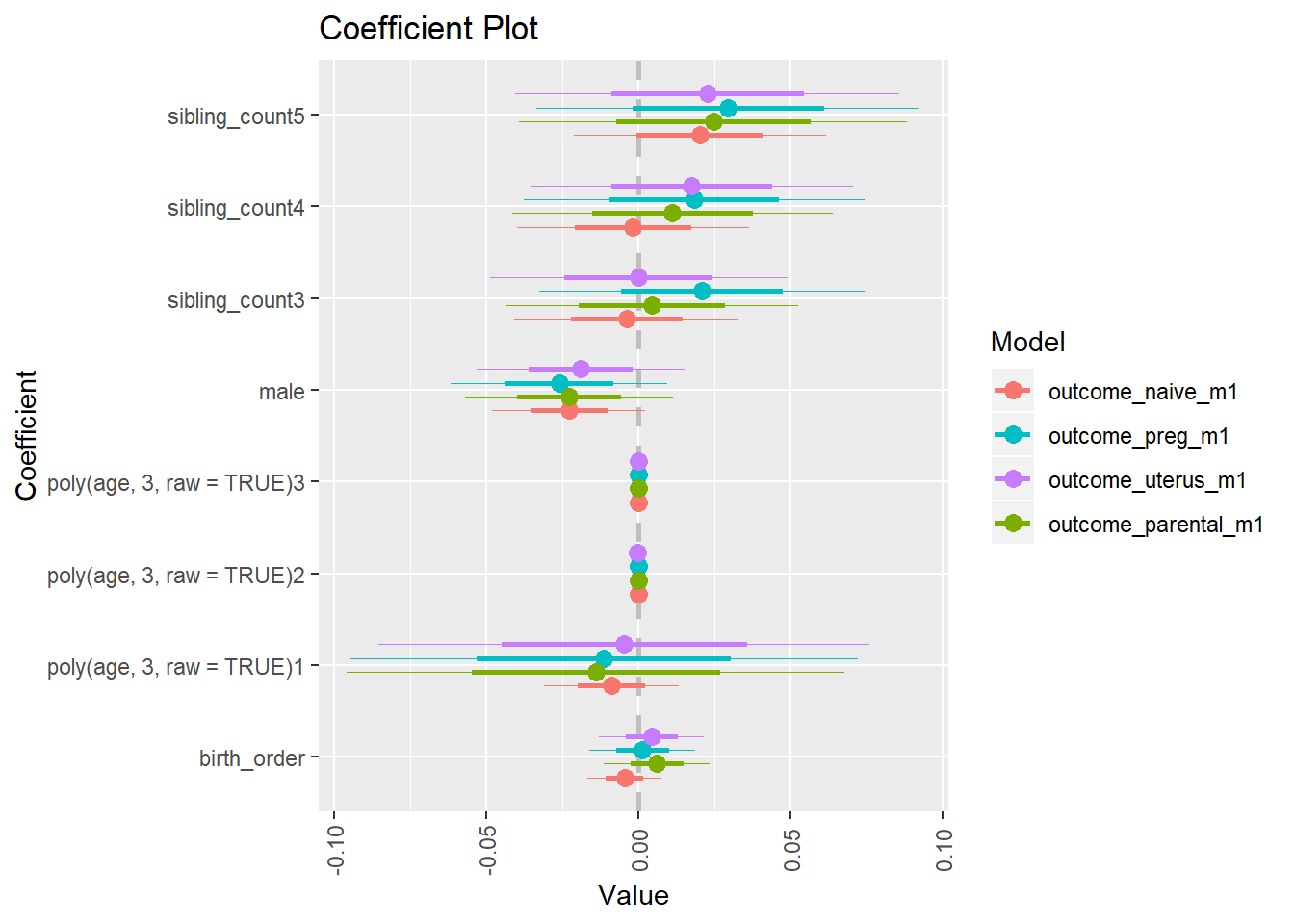
Sector_Mining and quarrying
birthorder <- birthorder %>% mutate(outcome = `Sector_Mining and quarrying`)
model = lmer(outcome ~ birth_order + poly(age, 3, raw = TRUE) + male + sibling_count + (1 | mother_pidlink),
data = birthorder)
compare_birthorder_specs(model)Naive birth order
outcome_naive_m1 <- update(m2_birthorder_linear, data = birthorder %>%
mutate(sibling_count = sibling_count_naive_factor,
birth_order_nonlinear = birthorder_naive_factor,
birth_order = birthorder_naive,
count_birth_order = count_birthorder_naive) %>%
filter(sibling_count != "1"))
compare_models_markdown(outcome_naive_m1)Basic Model
Model Summary
m1_covariates_only <- update(m2_birthorder_linear, formula = . ~ . - birth_order)
tidy(m1_covariates_only, conf.int = T, conf.level = 0.995)| effect | group | term | estimate | std.error | statistic | df | p.value | conf.low | conf.high |
|---|---|---|---|---|---|---|---|---|---|
| fixed | NA | (Intercept) | -0.04114 | 0.05247 | -0.7841 | 4234 | 0.433 | -0.1884 | 0.1061 |
| fixed | NA | poly(age, 3, raw = TRUE)1 | 0.003259 | 0.004667 | 0.6983 | 4106 | 0.485 | -0.009841 | 0.01636 |
| fixed | NA | poly(age, 3, raw = TRUE)2 | -0.00005486 | 0.0001292 | -0.4246 | 3964 | 0.6712 | -0.0004176 | 0.0003078 |
| fixed | NA | poly(age, 3, raw = TRUE)3 | 0.0000002653 | 0.000001127 | 0.2355 | 3839 | 0.8138 | -0.000002897 | 0.000003428 |
| fixed | NA | male | 0.03387 | 0.005354 | 6.326 | 4598 | 0.0000000002757 | 0.01884 | 0.04889 |
| fixed | NA | sibling_count3 | -0.0006718 | 0.00767 | -0.08759 | 3300 | 0.9302 | -0.0222 | 0.02086 |
| fixed | NA | sibling_count4 | 0.005238 | 0.007756 | 0.6754 | 3045 | 0.4995 | -0.01653 | 0.02701 |
| fixed | NA | sibling_count5 | 0.006951 | 0.008066 | 0.8618 | 2804 | 0.3889 | -0.01569 | 0.02959 |
| ran_pars | mother_pidlink | sd__(Intercept) | 0.05504 | NA | NA | NA | NA | NA | NA |
| ran_pars | Residual | sd__Observation | 0.1726 | NA | NA | NA | NA | NA | NA |
Coefficient Plot
plot(allEffects(m1_covariates_only, confidence.level = 0.995))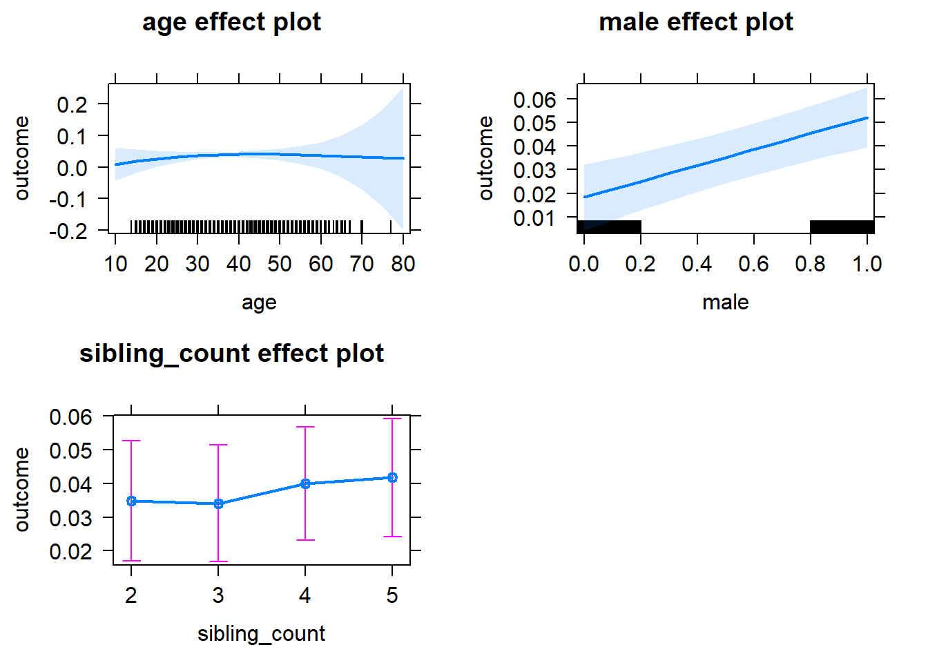
Add Birth Order Linear
Model Summary
tidy(m2_birthorder_linear, conf.int = T, conf.level = 0.995)| effect | group | term | estimate | std.error | statistic | df | p.value | conf.low | conf.high |
|---|---|---|---|---|---|---|---|---|---|
| fixed | NA | (Intercept) | -0.04073 | 0.05247 | -0.7763 | 4234 | 0.4376 | -0.188 | 0.1066 |
| fixed | NA | birth_order | 0.001501 | 0.002637 | 0.5691 | 4100 | 0.5693 | -0.005901 | 0.008902 |
| fixed | NA | poly(age, 3, raw = TRUE)1 | 0.003026 | 0.004685 | 0.6459 | 4108 | 0.5184 | -0.01013 | 0.01618 |
| fixed | NA | poly(age, 3, raw = TRUE)2 | -0.000049 | 0.0001296 | -0.378 | 3956 | 0.7054 | -0.0004129 | 0.0003149 |
| fixed | NA | poly(age, 3, raw = TRUE)3 | 0.0000002255 | 0.000001129 | 0.1998 | 3832 | 0.8417 | -0.000002943 | 0.000003394 |
| fixed | NA | male | 0.03389 | 0.005354 | 6.329 | 4597 | 0.0000000002699 | 0.01886 | 0.04892 |
| fixed | NA | sibling_count3 | -0.001236 | 0.007734 | -0.1598 | 3387 | 0.873 | -0.02294 | 0.02047 |
| fixed | NA | sibling_count4 | 0.004022 | 0.008044 | 0.5 | 3404 | 0.6171 | -0.01856 | 0.0266 |
| fixed | NA | sibling_count5 | 0.005029 | 0.008743 | 0.5752 | 3519 | 0.5652 | -0.01951 | 0.02957 |
| ran_pars | mother_pidlink | sd__(Intercept) | 0.05495 | NA | NA | NA | NA | NA | NA |
| ran_pars | Residual | sd__Observation | 0.1726 | NA | NA | NA | NA | NA | NA |
Coefficient Plot
plot_birthorder2(m2_birthorder_linear, separate = FALSE)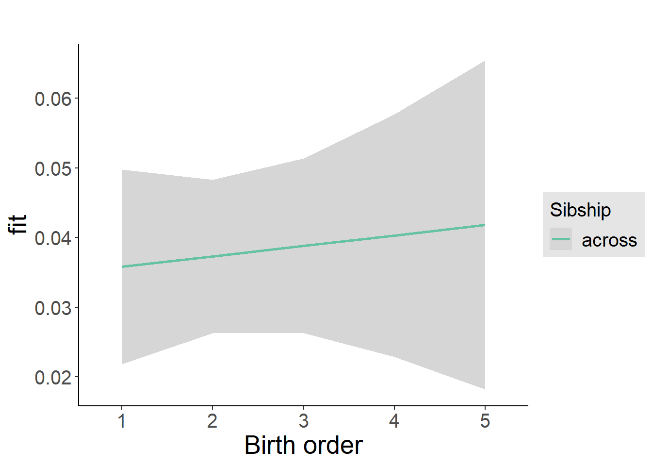
Add Birth Order Factor
Model Summary
m3_birthorder_nonlinear = update(m1_covariates_only, formula = . ~ . + birth_order_nonlinear)
tidy(m3_birthorder_nonlinear, conf.int = T, conf.level = 0.995)| effect | group | term | estimate | std.error | statistic | df | p.value | conf.low | conf.high |
|---|---|---|---|---|---|---|---|---|---|
| fixed | NA | (Intercept) | -0.04036 | 0.05264 | -0.7667 | 4240 | 0.4433 | -0.1881 | 0.1074 |
| fixed | NA | poly(age, 3, raw = TRUE)1 | 0.003043 | 0.004687 | 0.6493 | 4103 | 0.5162 | -0.01011 | 0.0162 |
| fixed | NA | poly(age, 3, raw = TRUE)2 | -0.00004848 | 0.0001297 | -0.3738 | 3947 | 0.7086 | -0.0004126 | 0.0003156 |
| fixed | NA | poly(age, 3, raw = TRUE)3 | 0.0000002116 | 0.00000113 | 0.1873 | 3816 | 0.8514 | -0.00000296 | 0.000003383 |
| fixed | NA | male | 0.03378 | 0.005355 | 6.308 | 4593 | 0.0000000003098 | 0.01875 | 0.04881 |
| fixed | NA | sibling_count3 | 0.00156 | 0.007869 | 0.1982 | 3539 | 0.8429 | -0.02053 | 0.02365 |
| fixed | NA | sibling_count4 | 0.005291 | 0.008192 | 0.6459 | 3570 | 0.5184 | -0.0177 | 0.02829 |
| fixed | NA | sibling_count5 | 0.005474 | 0.008832 | 0.6198 | 3614 | 0.5355 | -0.01932 | 0.03027 |
| fixed | NA | birth_order_nonlinear2 | 0.003364 | 0.006355 | 0.5294 | 4002 | 0.5966 | -0.01447 | 0.0212 |
| fixed | NA | birth_order_nonlinear3 | -0.00828 | 0.008056 | -1.028 | 3952 | 0.3041 | -0.03089 | 0.01433 |
| fixed | NA | birth_order_nonlinear4 | 0.01241 | 0.01052 | 1.179 | 3904 | 0.2384 | -0.01713 | 0.04195 |
| fixed | NA | birth_order_nonlinear5 | 0.01004 | 0.01519 | 0.6613 | 3965 | 0.5085 | -0.03259 | 0.05268 |
| ran_pars | mother_pidlink | sd__(Intercept) | 0.05526 | NA | NA | NA | NA | NA | NA |
| ran_pars | Residual | sd__Observation | 0.1725 | NA | NA | NA | NA | NA | NA |
Coefficient Plot
plot_birthorder(m3_birthorder_nonlinear, separate = FALSE)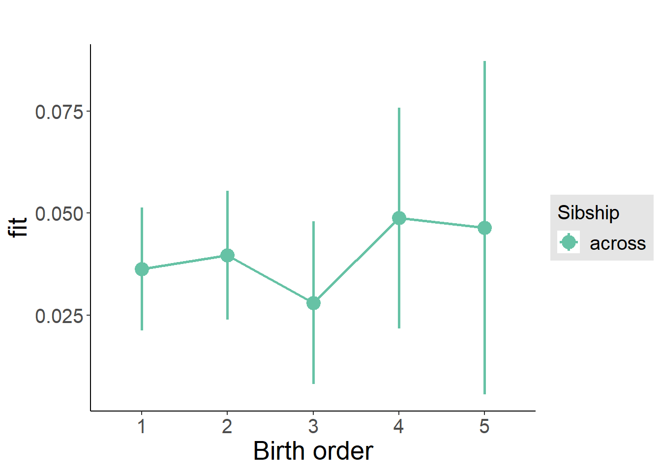
Add Interaction
Model Summary
m4_interaction = update(m3_birthorder_nonlinear, formula = . ~ . - birth_order_nonlinear - sibling_count + count_birth_order)
tidy(m4_interaction, conf.int = T, conf.level = 0.995)| effect | group | term | estimate | std.error | statistic | df | p.value | conf.low | conf.high |
|---|---|---|---|---|---|---|---|---|---|
| fixed | NA | (Intercept) | -0.04424 | 0.05271 | -0.8394 | 4245 | 0.4013 | -0.1922 | 0.1037 |
| fixed | NA | poly(age, 3, raw = TRUE)1 | 0.003113 | 0.004689 | 0.6638 | 4101 | 0.5069 | -0.01005 | 0.01628 |
| fixed | NA | poly(age, 3, raw = TRUE)2 | -0.00005035 | 0.0001297 | -0.3881 | 3945 | 0.6979 | -0.0004145 | 0.0003138 |
| fixed | NA | poly(age, 3, raw = TRUE)3 | 0.0000002263 | 0.00000113 | 0.2003 | 3814 | 0.8413 | -0.000002945 | 0.000003398 |
| fixed | NA | male | 0.03403 | 0.005356 | 6.353 | 4586 | 0.0000000002315 | 0.01899 | 0.04906 |
| fixed | NA | count_birth_order2/2 | 0.01135 | 0.01081 | 1.05 | 3927 | 0.2939 | -0.019 | 0.0417 |
| fixed | NA | count_birth_order1/3 | 0.005884 | 0.01037 | 0.5672 | 4617 | 0.5706 | -0.02323 | 0.035 |
| fixed | NA | count_birth_order2/3 | 0.01735 | 0.01155 | 1.503 | 4624 | 0.1329 | -0.01505 | 0.04976 |
| fixed | NA | count_birth_order3/3 | -0.01868 | 0.0127 | -1.47 | 4625 | 0.1415 | -0.05433 | 0.01698 |
| fixed | NA | count_birth_order1/4 | 0.01405 | 0.01143 | 1.229 | 4624 | 0.219 | -0.01803 | 0.04612 |
| fixed | NA | count_birth_order2/4 | -0.005288 | 0.01226 | -0.4314 | 4625 | 0.6662 | -0.0397 | 0.02912 |
| fixed | NA | count_birth_order3/4 | 0.009742 | 0.01294 | 0.753 | 4625 | 0.4515 | -0.02657 | 0.04605 |
| fixed | NA | count_birth_order4/4 | 0.02266 | 0.01395 | 1.625 | 4624 | 0.1043 | -0.01649 | 0.06181 |
| fixed | NA | count_birth_order1/5 | 0.005603 | 0.01288 | 0.4348 | 4624 | 0.6637 | -0.03056 | 0.04177 |
| fixed | NA | count_birth_order2/5 | 0.009956 | 0.01369 | 0.7272 | 4622 | 0.4671 | -0.02848 | 0.04839 |
| fixed | NA | count_birth_order3/5 | 0.008266 | 0.0144 | 0.5739 | 4619 | 0.566 | -0.03216 | 0.0487 |
| fixed | NA | count_birth_order4/5 | 0.01827 | 0.01522 | 1.201 | 4608 | 0.2298 | -0.02444 | 0.06099 |
| fixed | NA | count_birth_order5/5 | 0.01856 | 0.01526 | 1.216 | 4618 | 0.224 | -0.02427 | 0.06138 |
| ran_pars | mother_pidlink | sd__(Intercept) | 0.05503 | NA | NA | NA | NA | NA | NA |
| ran_pars | Residual | sd__Observation | 0.1725 | NA | NA | NA | NA | NA | NA |
Coefficient Plot
plot_birthorder(m4_interaction)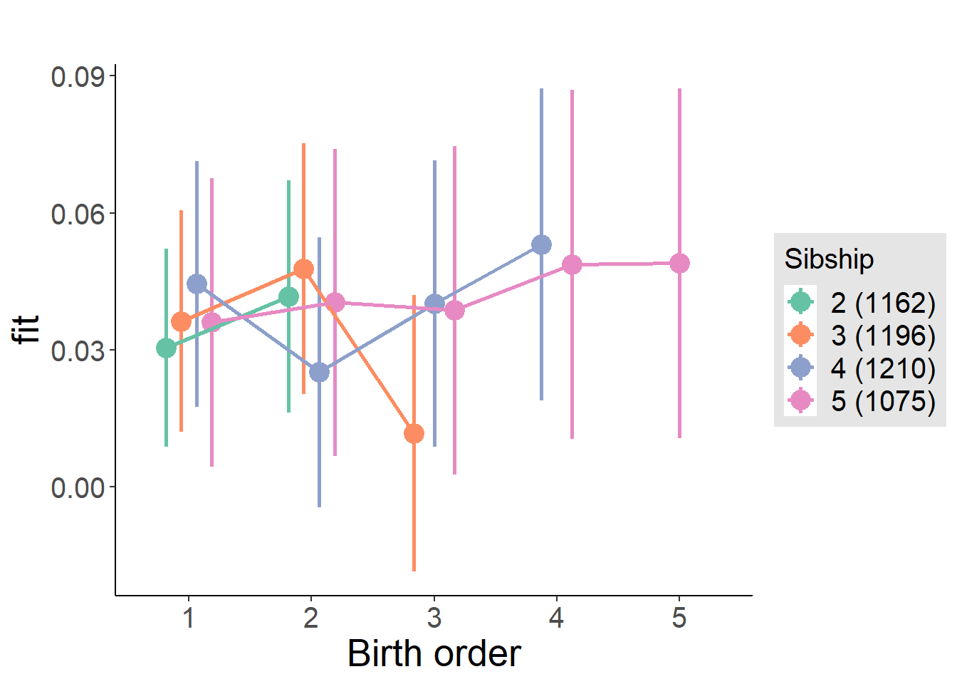
Model Comparison
###### Model 1 - Model 2
anova(m1_covariates_only, m2_birthorder_linear, m3_birthorder_nonlinear, m4_interaction)## refitting model(s) with ML (instead of REML)| Df | AIC | BIC | logLik | deviance | Chisq | Chi Df | Pr(>Chisq) |
|---|---|---|---|---|---|---|---|
| 10 | -2693 | -2629 | 1357 | -2713 | NA | NA | NA |
| 11 | -2692 | -2621 | 1357 | -2714 | 0.3253 | 1 | 0.5685 |
| 14 | -2690 | -2599 | 1359 | -2718 | 3.947 | 3 | 0.2672 |
| 20 | -2686 | -2557 | 1363 | -2726 | 8.434 | 6 | 0.208 |
Maternal birth order
outcome_uterus_m1 <- update(m2_birthorder_linear, data = birthorder %>%
mutate(sibling_count = sibling_count_uterus_alive_factor,
birth_order_nonlinear = birthorder_uterus_alive_factor,
birth_order = birthorder_uterus_alive,
count_birth_order = count_birthorder_uterus_alive) %>%
filter(sibling_count != "1"))
compare_models_markdown(outcome_uterus_m1)Basic Model
Model Summary
m1_covariates_only <- update(m2_birthorder_linear, formula = . ~ . - birth_order)
tidy(m1_covariates_only, conf.int = T, conf.level = 0.995)| effect | group | term | estimate | std.error | statistic | df | p.value | conf.low | conf.high |
|---|---|---|---|---|---|---|---|---|---|
| fixed | NA | (Intercept) | -0.05793 | 0.1314 | -0.4408 | 2617 | 0.6594 | -0.4268 | 0.311 |
| fixed | NA | poly(age, 3, raw = TRUE)1 | 0.006296 | 0.01454 | 0.4329 | 2616 | 0.6651 | -0.03453 | 0.04712 |
| fixed | NA | poly(age, 3, raw = TRUE)2 | -0.0002183 | 0.0005152 | -0.4237 | 2613 | 0.6718 | -0.001664 | 0.001228 |
| fixed | NA | poly(age, 3, raw = TRUE)3 | 0.000002348 | 0.000005844 | 0.4018 | 2610 | 0.6878 | -0.00001406 | 0.00001875 |
| fixed | NA | male | 0.02987 | 0.006185 | 4.83 | 2632 | 0.000001447 | 0.01251 | 0.04723 |
| fixed | NA | sibling_count3 | 0.01389 | 0.008552 | 1.624 | 1997 | 0.1046 | -0.01012 | 0.03789 |
| fixed | NA | sibling_count4 | 0.01745 | 0.008839 | 1.974 | 1772 | 0.0485 | -0.00736 | 0.04226 |
| fixed | NA | sibling_count5 | 0.005046 | 0.009832 | 0.5132 | 1469 | 0.6079 | -0.02255 | 0.03264 |
| ran_pars | mother_pidlink | sd__(Intercept) | 0.03304 | NA | NA | NA | NA | NA | NA |
| ran_pars | Residual | sd__Observation | 0.1531 | NA | NA | NA | NA | NA | NA |
Coefficient Plot
plot(allEffects(m1_covariates_only, confidence.level = 0.995))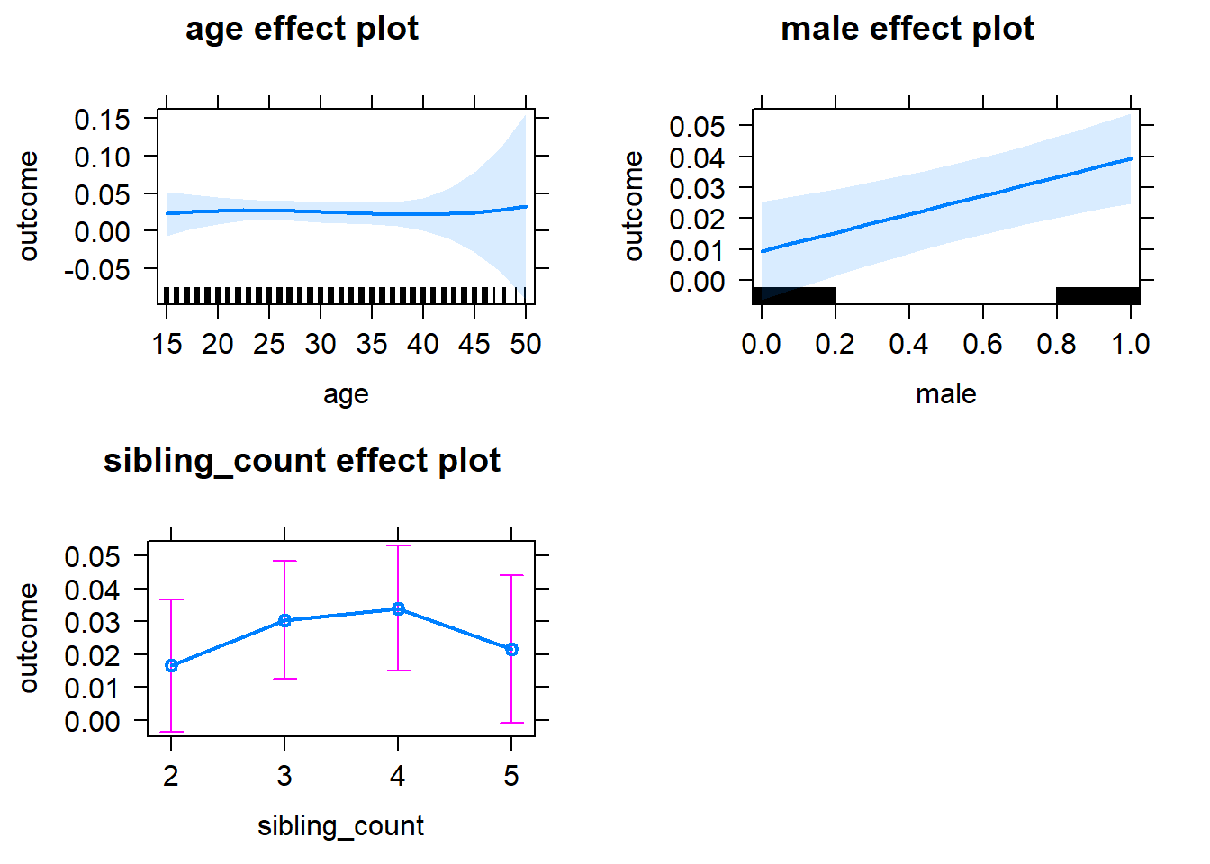
Add Birth Order Linear
Model Summary
tidy(m2_birthorder_linear, conf.int = T, conf.level = 0.995)| effect | group | term | estimate | std.error | statistic | df | p.value | conf.low | conf.high |
|---|---|---|---|---|---|---|---|---|---|
| fixed | NA | (Intercept) | -0.05741 | 0.1314 | -0.4369 | 2616 | 0.6622 | -0.4263 | 0.3115 |
| fixed | NA | birth_order | -0.003042 | 0.003126 | -0.9732 | 2485 | 0.3306 | -0.01182 | 0.005732 |
| fixed | NA | poly(age, 3, raw = TRUE)1 | 0.006589 | 0.01455 | 0.4529 | 2614 | 0.6506 | -0.03425 | 0.04742 |
| fixed | NA | poly(age, 3, raw = TRUE)2 | -0.0002234 | 0.0005152 | -0.4336 | 2612 | 0.6646 | -0.00167 | 0.001223 |
| fixed | NA | poly(age, 3, raw = TRUE)3 | 0.000002329 | 0.000005844 | 0.3985 | 2610 | 0.6903 | -0.00001408 | 0.00001873 |
| fixed | NA | male | 0.02987 | 0.006185 | 4.829 | 2631 | 0.000001448 | 0.01251 | 0.04723 |
| fixed | NA | sibling_count3 | 0.01533 | 0.00868 | 1.766 | 2032 | 0.07761 | -0.009039 | 0.03969 |
| fixed | NA | sibling_count4 | 0.02056 | 0.009399 | 2.187 | 1917 | 0.02884 | -0.005824 | 0.04694 |
| fixed | NA | sibling_count5 | 0.01022 | 0.01119 | 0.9141 | 1830 | 0.3608 | -0.02117 | 0.04162 |
| ran_pars | mother_pidlink | sd__(Intercept) | 0.03344 | NA | NA | NA | NA | NA | NA |
| ran_pars | Residual | sd__Observation | 0.153 | NA | NA | NA | NA | NA | NA |
Coefficient Plot
plot_birthorder2(m2_birthorder_linear, separate = FALSE)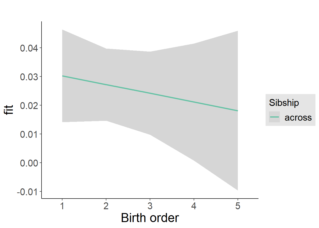
Add Birth Order Factor
Model Summary
m3_birthorder_nonlinear = update(m1_covariates_only, formula = . ~ . + birth_order_nonlinear)
tidy(m3_birthorder_nonlinear, conf.int = T, conf.level = 0.995)| effect | group | term | estimate | std.error | statistic | df | p.value | conf.low | conf.high |
|---|---|---|---|---|---|---|---|---|---|
| fixed | NA | (Intercept) | -0.05802 | 0.1317 | -0.4404 | 2611 | 0.6597 | -0.4278 | 0.3118 |
| fixed | NA | poly(age, 3, raw = TRUE)1 | 0.006437 | 0.01458 | 0.4416 | 2610 | 0.6588 | -0.03448 | 0.04735 |
| fixed | NA | poly(age, 3, raw = TRUE)2 | -0.0002174 | 0.0005162 | -0.4212 | 2608 | 0.6736 | -0.001666 | 0.001232 |
| fixed | NA | poly(age, 3, raw = TRUE)3 | 0.000002259 | 0.000005854 | 0.3859 | 2606 | 0.6996 | -0.00001417 | 0.00001869 |
| fixed | NA | male | 0.02985 | 0.006193 | 4.819 | 2629 | 0.000001522 | 0.01246 | 0.04723 |
| fixed | NA | sibling_count3 | 0.01552 | 0.008817 | 1.76 | 2104 | 0.07848 | -0.009228 | 0.04027 |
| fixed | NA | sibling_count4 | 0.02093 | 0.009533 | 2.196 | 1984 | 0.02823 | -0.005828 | 0.04769 |
| fixed | NA | sibling_count5 | 0.008965 | 0.01133 | 0.7912 | 1880 | 0.4289 | -0.02284 | 0.04077 |
| fixed | NA | birth_order_nonlinear2 | -0.006992 | 0.007484 | -0.9343 | 2240 | 0.3503 | -0.028 | 0.01402 |
| fixed | NA | birth_order_nonlinear3 | -0.007257 | 0.00912 | -0.7957 | 2306 | 0.4263 | -0.03286 | 0.01834 |
| fixed | NA | birth_order_nonlinear4 | -0.0112 | 0.01214 | -0.9224 | 2391 | 0.3564 | -0.04527 | 0.02287 |
| fixed | NA | birth_order_nonlinear5 | -0.005136 | 0.01882 | -0.273 | 2330 | 0.7849 | -0.05795 | 0.04768 |
| ran_pars | mother_pidlink | sd__(Intercept) | 0.03315 | NA | NA | NA | NA | NA | NA |
| ran_pars | Residual | sd__Observation | 0.1532 | NA | NA | NA | NA | NA | NA |
Coefficient Plot
plot_birthorder(m3_birthorder_nonlinear, separate = FALSE)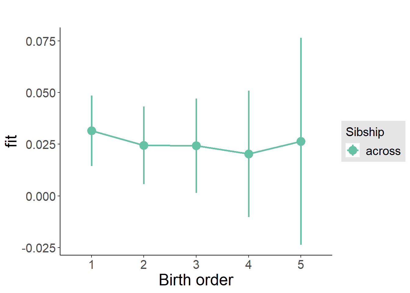
Add Interaction
Model Summary
m4_interaction = update(m3_birthorder_nonlinear, formula = . ~ . - birth_order_nonlinear - sibling_count + count_birth_order)
tidy(m4_interaction, conf.int = T, conf.level = 0.995)| effect | group | term | estimate | std.error | statistic | df | p.value | conf.low | conf.high |
|---|---|---|---|---|---|---|---|---|---|
| fixed | NA | (Intercept) | -0.05972 | 0.1319 | -0.4528 | 2606 | 0.6507 | -0.4299 | 0.3105 |
| fixed | NA | poly(age, 3, raw = TRUE)1 | 0.006849 | 0.01459 | 0.4694 | 2605 | 0.6388 | -0.03411 | 0.04781 |
| fixed | NA | poly(age, 3, raw = TRUE)2 | -0.0002286 | 0.0005168 | -0.4422 | 2603 | 0.6583 | -0.001679 | 0.001222 |
| fixed | NA | poly(age, 3, raw = TRUE)3 | 0.000002352 | 0.000005863 | 0.4012 | 2601 | 0.6883 | -0.00001411 | 0.00001881 |
| fixed | NA | male | 0.03006 | 0.006203 | 4.845 | 2622 | 0.000001339 | 0.01264 | 0.04747 |
| fixed | NA | count_birth_order2/2 | -0.01628 | 0.01365 | -1.193 | 2223 | 0.233 | -0.05459 | 0.02203 |
| fixed | NA | count_birth_order1/3 | 0.007834 | 0.01136 | 0.6895 | 2623 | 0.4906 | -0.02406 | 0.03973 |
| fixed | NA | count_birth_order2/3 | 0.01593 | 0.01263 | 1.261 | 2624 | 0.2072 | -0.01952 | 0.05138 |
| fixed | NA | count_birth_order3/3 | 0.0004743 | 0.01376 | 0.03446 | 2622 | 0.9725 | -0.03816 | 0.03911 |
| fixed | NA | count_birth_order1/4 | 0.01964 | 0.01307 | 1.502 | 2624 | 0.1332 | -0.01706 | 0.05633 |
| fixed | NA | count_birth_order2/4 | 0.005646 | 0.01384 | 0.4079 | 2624 | 0.6834 | -0.0332 | 0.04449 |
| fixed | NA | count_birth_order3/4 | 0.009496 | 0.01435 | 0.6616 | 2621 | 0.5083 | -0.0308 | 0.04979 |
| fixed | NA | count_birth_order4/4 | 0.01226 | 0.01535 | 0.7987 | 2622 | 0.4246 | -0.03082 | 0.05534 |
| fixed | NA | count_birth_order1/5 | 0.006802 | 0.01726 | 0.3941 | 2624 | 0.6936 | -0.04165 | 0.05526 |
| fixed | NA | count_birth_order2/5 | -0.005763 | 0.01858 | -0.3102 | 2622 | 0.7564 | -0.05791 | 0.04638 |
| fixed | NA | count_birth_order3/5 | 0.009764 | 0.01764 | 0.5534 | 2620 | 0.58 | -0.03976 | 0.05929 |
| fixed | NA | count_birth_order4/5 | -0.01283 | 0.0172 | -0.7459 | 2618 | 0.4558 | -0.0611 | 0.03544 |
| fixed | NA | count_birth_order5/5 | 0.0007238 | 0.01809 | 0.04001 | 2615 | 0.9681 | -0.05006 | 0.05151 |
| ran_pars | mother_pidlink | sd__(Intercept) | 0.03326 | NA | NA | NA | NA | NA | NA |
| ran_pars | Residual | sd__Observation | 0.1532 | NA | NA | NA | NA | NA | NA |
Coefficient Plot
plot_birthorder(m4_interaction)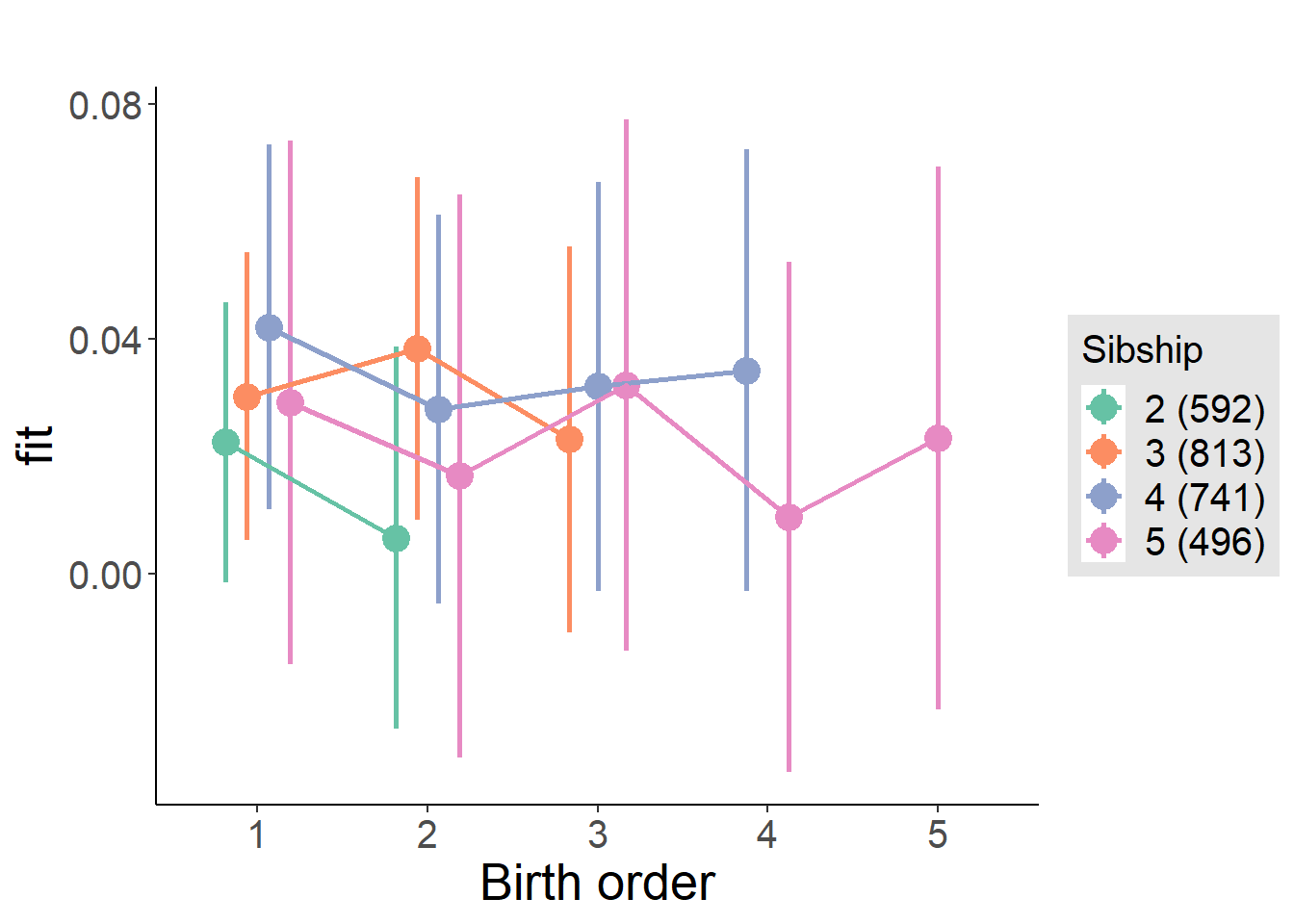
Model Comparison
###### Model 1 - Model 2
anova(m1_covariates_only, m2_birthorder_linear, m3_birthorder_nonlinear, m4_interaction)## refitting model(s) with ML (instead of REML)| Df | AIC | BIC | logLik | deviance | Chisq | Chi Df | Pr(>Chisq) |
|---|---|---|---|---|---|---|---|
| 10 | -2288 | -2229 | 1154 | -2308 | NA | NA | NA |
| 11 | -2287 | -2222 | 1154 | -2309 | 0.9458 | 1 | 0.3308 |
| 14 | -2281 | -2199 | 1155 | -2309 | 0.5254 | 3 | 0.9133 |
| 20 | -2273 | -2155 | 1156 | -2313 | 3.4 | 6 | 0.7572 |
Maternal pregnancy order
outcome_preg_m1 <- update(m2_birthorder_linear, data = birthorder %>%
mutate(sibling_count = sibling_count_uterus_preg_factor,
birth_order_nonlinear = birthorder_uterus_preg_factor,
birth_order = birthorder_uterus_preg,
count_birth_order = count_birthorder_uterus_preg
) %>%
filter(sibling_count != "1"))
compare_models_markdown(outcome_preg_m1)Basic Model
Model Summary
m1_covariates_only <- update(m2_birthorder_linear, formula = . ~ . - birth_order)
tidy(m1_covariates_only, conf.int = T, conf.level = 0.995)| effect | group | term | estimate | std.error | statistic | df | p.value | conf.low | conf.high |
|---|---|---|---|---|---|---|---|---|---|
| fixed | NA | (Intercept) | -0.07806 | 0.1354 | -0.5767 | 2408 | 0.5642 | -0.458 | 0.3019 |
| fixed | NA | poly(age, 3, raw = TRUE)1 | 0.008781 | 0.01499 | 0.5858 | 2408 | 0.5581 | -0.0333 | 0.05086 |
| fixed | NA | poly(age, 3, raw = TRUE)2 | -0.0003152 | 0.000531 | -0.5936 | 2406 | 0.5528 | -0.001806 | 0.001175 |
| fixed | NA | poly(age, 3, raw = TRUE)3 | 0.000003566 | 0.000006024 | 0.592 | 2404 | 0.5539 | -0.00001334 | 0.00002047 |
| fixed | NA | male | 0.03138 | 0.00642 | 4.888 | 2418 | 0.000001086 | 0.01336 | 0.0494 |
| fixed | NA | sibling_count3 | 0.00778 | 0.009328 | 0.8341 | 1938 | 0.4043 | -0.0184 | 0.03396 |
| fixed | NA | sibling_count4 | 0.02212 | 0.00943 | 2.346 | 1812 | 0.0191 | -0.004351 | 0.04859 |
| fixed | NA | sibling_count5 | -0.0002185 | 0.009928 | -0.02201 | 1632 | 0.9824 | -0.02809 | 0.02765 |
| ran_pars | mother_pidlink | sd__(Intercept) | 0.03196 | NA | NA | NA | NA | NA | NA |
| ran_pars | Residual | sd__Observation | 0.1524 | NA | NA | NA | NA | NA | NA |
Coefficient Plot
plot(allEffects(m1_covariates_only, confidence.level = 0.995))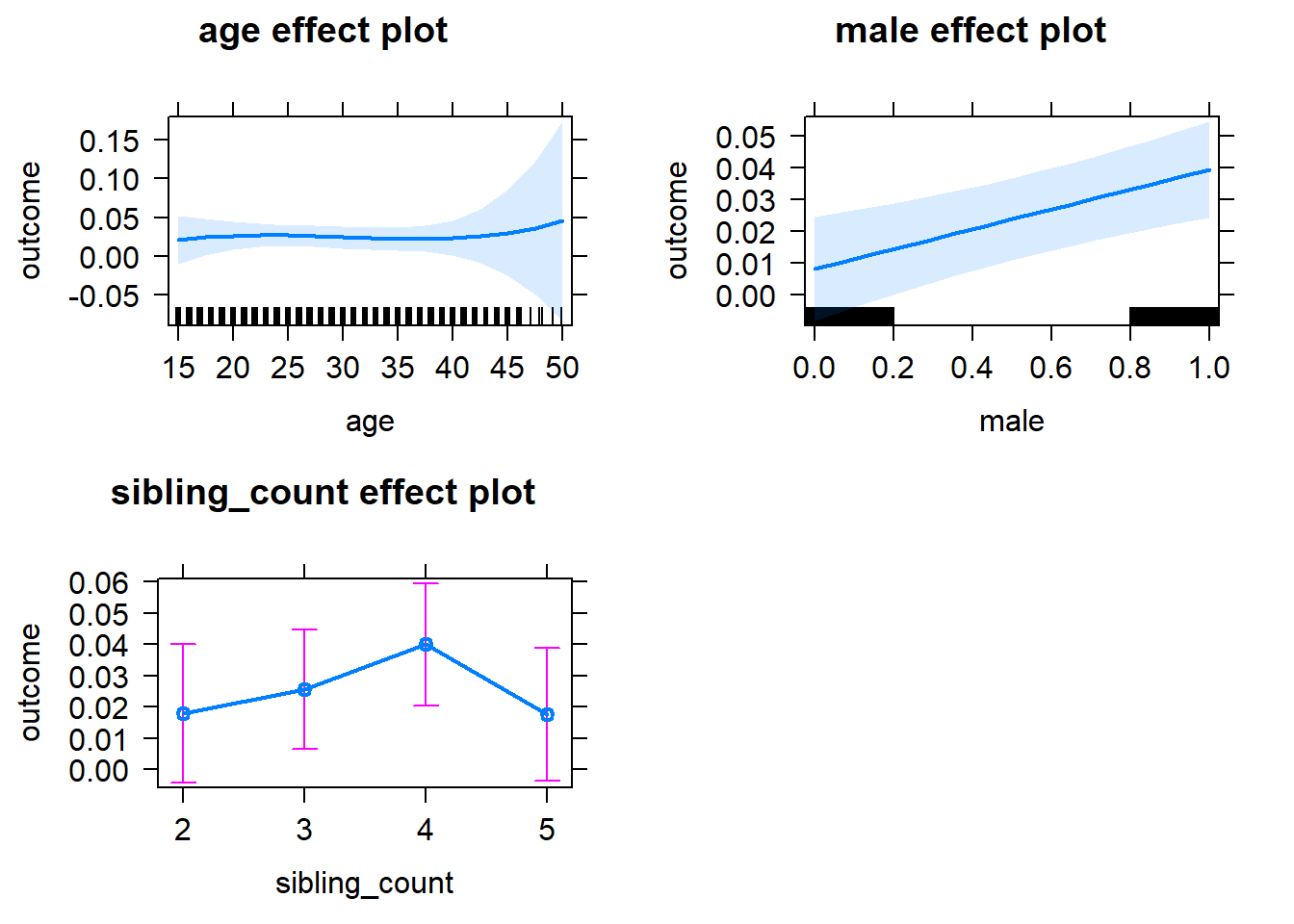
Add Birth Order Linear
Model Summary
tidy(m2_birthorder_linear, conf.int = T, conf.level = 0.995)| effect | group | term | estimate | std.error | statistic | df | p.value | conf.low | conf.high |
|---|---|---|---|---|---|---|---|---|---|
| fixed | NA | (Intercept) | -0.07547 | 0.1354 | -0.5575 | 2408 | 0.5773 | -0.4555 | 0.3045 |
| fixed | NA | birth_order | -0.003698 | 0.003151 | -1.174 | 2353 | 0.2406 | -0.01254 | 0.005147 |
| fixed | NA | poly(age, 3, raw = TRUE)1 | 0.008972 | 0.01499 | 0.5985 | 2407 | 0.5496 | -0.03311 | 0.05105 |
| fixed | NA | poly(age, 3, raw = TRUE)2 | -0.0003171 | 0.0005309 | -0.5972 | 2405 | 0.5505 | -0.001807 | 0.001173 |
| fixed | NA | poly(age, 3, raw = TRUE)3 | 0.000003505 | 0.000006024 | 0.5819 | 2403 | 0.5607 | -0.0000134 | 0.00002041 |
| fixed | NA | male | 0.03128 | 0.00642 | 4.873 | 2417 | 0.000001173 | 0.01326 | 0.0493 |
| fixed | NA | sibling_count3 | 0.009543 | 0.009448 | 1.01 | 1957 | 0.3126 | -0.01698 | 0.03606 |
| fixed | NA | sibling_count4 | 0.0256 | 0.009887 | 2.59 | 1894 | 0.009676 | -0.002148 | 0.05336 |
| fixed | NA | sibling_count5 | 0.005673 | 0.01113 | 0.5097 | 1877 | 0.6103 | -0.02557 | 0.03691 |
| ran_pars | mother_pidlink | sd__(Intercept) | 0.03238 | NA | NA | NA | NA | NA | NA |
| ran_pars | Residual | sd__Observation | 0.1523 | NA | NA | NA | NA | NA | NA |
Coefficient Plot
plot_birthorder2(m2_birthorder_linear, separate = FALSE)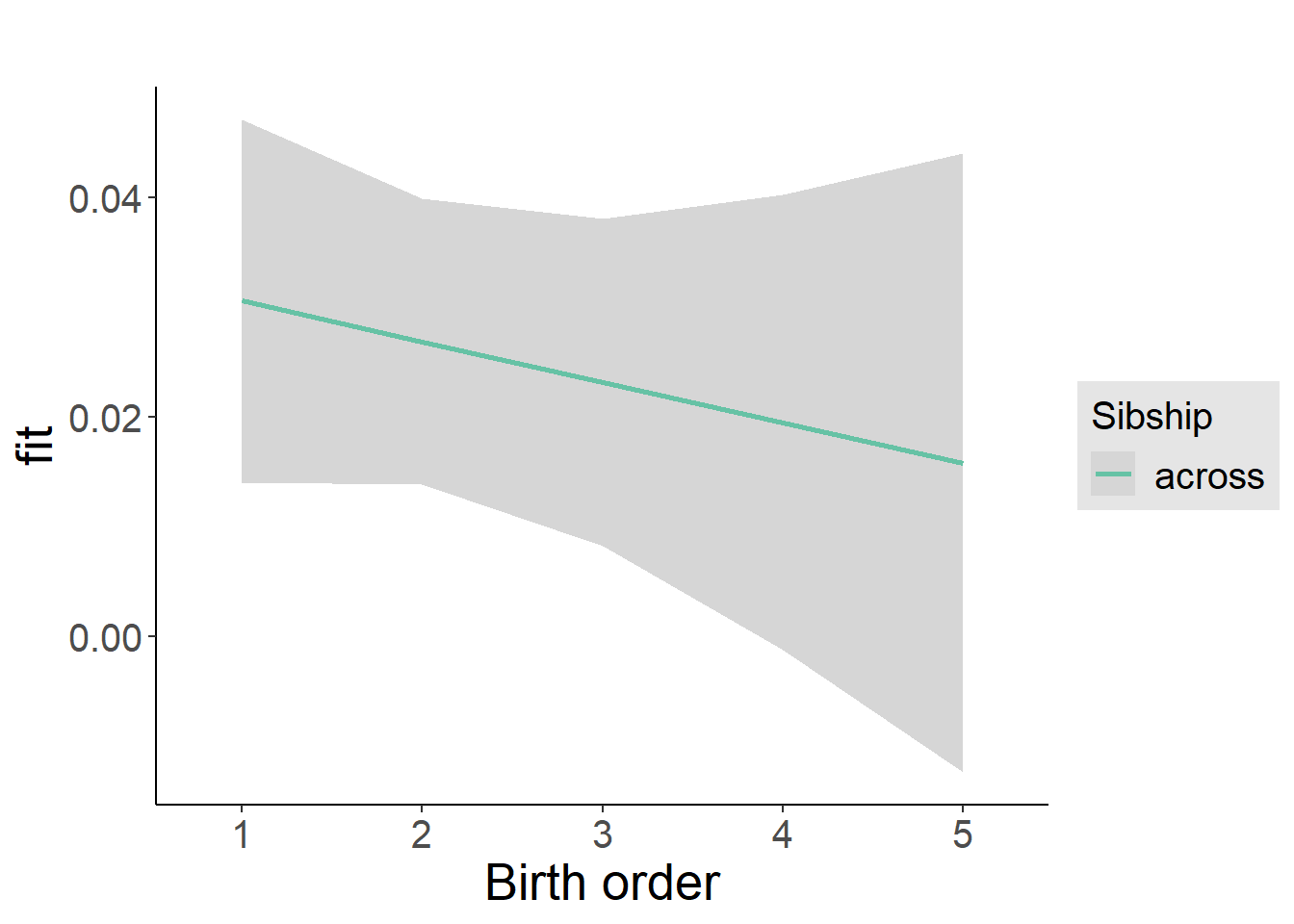
Add Birth Order Factor
Model Summary
m3_birthorder_nonlinear = update(m1_covariates_only, formula = . ~ . + birth_order_nonlinear)
tidy(m3_birthorder_nonlinear, conf.int = T, conf.level = 0.995)| effect | group | term | estimate | std.error | statistic | df | p.value | conf.low | conf.high |
|---|---|---|---|---|---|---|---|---|---|
| fixed | NA | (Intercept) | -0.07254 | 0.1357 | -0.5344 | 2402 | 0.5931 | -0.4536 | 0.3085 |
| fixed | NA | poly(age, 3, raw = TRUE)1 | 0.008351 | 0.01503 | 0.5556 | 2402 | 0.5785 | -0.03384 | 0.05054 |
| fixed | NA | poly(age, 3, raw = TRUE)2 | -0.0002951 | 0.0005323 | -0.5543 | 2400 | 0.5794 | -0.001789 | 0.001199 |
| fixed | NA | poly(age, 3, raw = TRUE)3 | 0.000003262 | 0.000006038 | 0.5403 | 2399 | 0.589 | -0.00001369 | 0.00002021 |
| fixed | NA | male | 0.03128 | 0.006427 | 4.867 | 2414 | 0.000001208 | 0.01324 | 0.04932 |
| fixed | NA | sibling_count3 | 0.01042 | 0.009587 | 1.086 | 2008 | 0.2774 | -0.0165 | 0.03733 |
| fixed | NA | sibling_count4 | 0.02687 | 0.01002 | 2.683 | 1941 | 0.007359 | -0.001242 | 0.05498 |
| fixed | NA | sibling_count5 | 0.004529 | 0.0112 | 0.4042 | 1903 | 0.6861 | -0.02692 | 0.03598 |
| fixed | NA | birth_order_nonlinear2 | -0.007134 | 0.007718 | -0.9244 | 2111 | 0.3554 | -0.0288 | 0.01453 |
| fixed | NA | birth_order_nonlinear3 | -0.01143 | 0.009499 | -1.203 | 2210 | 0.229 | -0.0381 | 0.01523 |
| fixed | NA | birth_order_nonlinear4 | -0.01486 | 0.01253 | -1.186 | 2279 | 0.2357 | -0.05002 | 0.02031 |
| fixed | NA | birth_order_nonlinear5 | -0.002616 | 0.018 | -0.1453 | 2210 | 0.8845 | -0.05314 | 0.04791 |
| ran_pars | mother_pidlink | sd__(Intercept) | 0.03216 | NA | NA | NA | NA | NA | NA |
| ran_pars | Residual | sd__Observation | 0.1524 | NA | NA | NA | NA | NA | NA |
Coefficient Plot
plot_birthorder(m3_birthorder_nonlinear, separate = FALSE)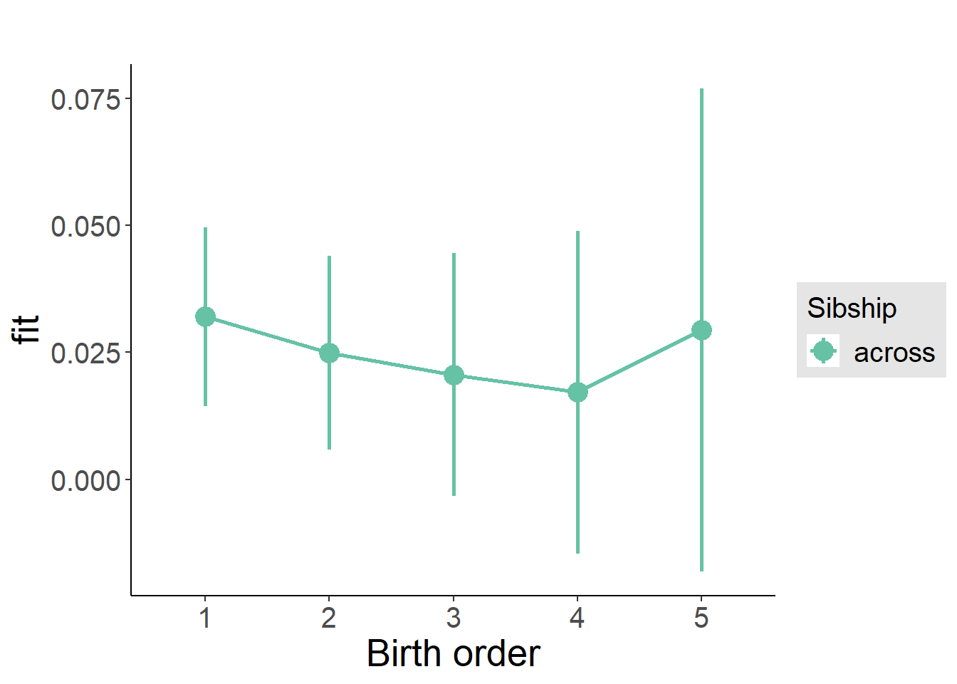
Add Interaction
Model Summary
m4_interaction = update(m3_birthorder_nonlinear, formula = . ~ . - birth_order_nonlinear - sibling_count + count_birth_order)
tidy(m4_interaction, conf.int = T, conf.level = 0.995)| effect | group | term | estimate | std.error | statistic | df | p.value | conf.low | conf.high |
|---|---|---|---|---|---|---|---|---|---|
| fixed | NA | (Intercept) | -0.07761 | 0.136 | -0.5708 | 2397 | 0.5682 | -0.4592 | 0.304 |
| fixed | NA | poly(age, 3, raw = TRUE)1 | 0.009171 | 0.01505 | 0.6093 | 2396 | 0.5424 | -0.03308 | 0.05142 |
| fixed | NA | poly(age, 3, raw = TRUE)2 | -0.0003208 | 0.0005332 | -0.6018 | 2394 | 0.5474 | -0.001817 | 0.001176 |
| fixed | NA | poly(age, 3, raw = TRUE)3 | 0.000003526 | 0.000006048 | 0.583 | 2392 | 0.5599 | -0.00001345 | 0.0000205 |
| fixed | NA | male | 0.03181 | 0.006443 | 4.937 | 2408 | 0.0000008484 | 0.01372 | 0.04989 |
| fixed | NA | count_birth_order2/2 | -0.01758 | 0.01487 | -1.182 | 2140 | 0.2373 | -0.05934 | 0.02417 |
| fixed | NA | count_birth_order1/3 | -0.001176 | 0.0125 | -0.09409 | 2408 | 0.925 | -0.03626 | 0.03391 |
| fixed | NA | count_birth_order2/3 | 0.01443 | 0.0136 | 1.061 | 2409 | 0.2889 | -0.02375 | 0.05262 |
| fixed | NA | count_birth_order3/3 | -0.009638 | 0.01508 | -0.6389 | 2407 | 0.5229 | -0.05198 | 0.03271 |
| fixed | NA | count_birth_order1/4 | 0.02995 | 0.01361 | 2.201 | 2408 | 0.0278 | -0.008241 | 0.06815 |
| fixed | NA | count_birth_order2/4 | 0.008284 | 0.01432 | 0.5786 | 2409 | 0.5629 | -0.03191 | 0.04848 |
| fixed | NA | count_birth_order3/4 | 0.01229 | 0.0155 | 0.793 | 2407 | 0.4279 | -0.03121 | 0.05578 |
| fixed | NA | count_birth_order4/4 | 0.007536 | 0.01681 | 0.4483 | 2407 | 0.654 | -0.03965 | 0.05473 |
| fixed | NA | count_birth_order1/5 | -0.0008688 | 0.01648 | -0.05273 | 2409 | 0.958 | -0.04712 | 0.04538 |
| fixed | NA | count_birth_order2/5 | -0.01143 | 0.01687 | -0.6776 | 2409 | 0.4981 | -0.05878 | 0.03592 |
| fixed | NA | count_birth_order3/5 | -0.003623 | 0.01734 | -0.2089 | 2406 | 0.8345 | -0.0523 | 0.04506 |
| fixed | NA | count_birth_order4/5 | -0.01296 | 0.01762 | -0.7354 | 2405 | 0.4621 | -0.06242 | 0.0365 |
| fixed | NA | count_birth_order5/5 | -0.001646 | 0.01789 | -0.09197 | 2401 | 0.9267 | -0.05187 | 0.04858 |
| ran_pars | mother_pidlink | sd__(Intercept) | 0.03227 | NA | NA | NA | NA | NA | NA |
| ran_pars | Residual | sd__Observation | 0.1525 | NA | NA | NA | NA | NA | NA |
Coefficient Plot
plot_birthorder(m4_interaction)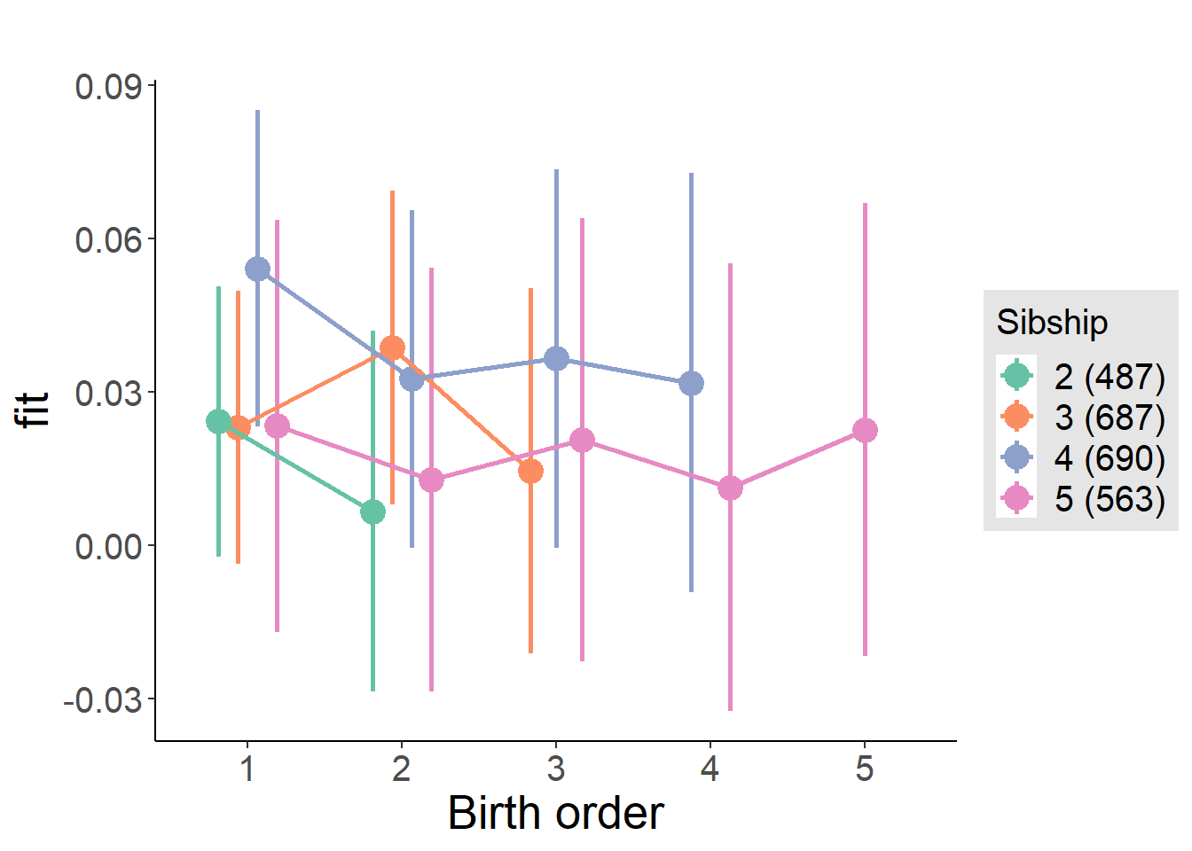
Model Comparison
###### Model 1 - Model 2
anova(m1_covariates_only, m2_birthorder_linear, m3_birthorder_nonlinear, m4_interaction)## refitting model(s) with ML (instead of REML)| Df | AIC | BIC | logLik | deviance | Chisq | Chi Df | Pr(>Chisq) |
|---|---|---|---|---|---|---|---|
| 10 | -2128 | -2070 | 1074 | -2148 | NA | NA | NA |
| 11 | -2127 | -2064 | 1075 | -2149 | 1.378 | 1 | 0.2405 |
| 14 | -2122 | -2041 | 1075 | -2150 | 1.057 | 3 | 0.7874 |
| 20 | -2115 | -1999 | 1078 | -2155 | 4.807 | 6 | 0.5688 |
Parental full sibling order
outcome_parental_m1 <- update(m2_birthorder_linear, data = birthorder %>%
mutate(sibling_count = sibling_count_genes_factor,
birth_order_nonlinear = birthorder_genes_factor,
birth_order = birthorder_genes,
count_birth_order = count_birthorder_genes
) %>%
filter(sibling_count != "1"))
compare_models_markdown(outcome_parental_m1)Basic Model
Model Summary
m1_covariates_only <- update(m2_birthorder_linear, formula = . ~ . - birth_order)
tidy(m1_covariates_only, conf.int = T, conf.level = 0.995)| effect | group | term | estimate | std.error | statistic | df | p.value | conf.low | conf.high |
|---|---|---|---|---|---|---|---|---|---|
| fixed | NA | (Intercept) | -0.05874 | 0.1336 | -0.4396 | 2615 | 0.6603 | -0.4338 | 0.3163 |
| fixed | NA | poly(age, 3, raw = TRUE)1 | 0.006903 | 0.01483 | 0.4655 | 2614 | 0.6416 | -0.03472 | 0.04853 |
| fixed | NA | poly(age, 3, raw = TRUE)2 | -0.0002496 | 0.0005265 | -0.4741 | 2611 | 0.6355 | -0.001727 | 0.001228 |
| fixed | NA | poly(age, 3, raw = TRUE)3 | 0.00000279 | 0.000005988 | 0.4659 | 2608 | 0.6413 | -0.00001402 | 0.0000196 |
| fixed | NA | male | 0.02883 | 0.006223 | 4.633 | 2635 | 0.000003787 | 0.01136 | 0.0463 |
| fixed | NA | sibling_count3 | 0.01377 | 0.00844 | 1.632 | 1928 | 0.1029 | -0.009918 | 0.03747 |
| fixed | NA | sibling_count4 | 0.01583 | 0.008845 | 1.79 | 1698 | 0.07363 | -0.008996 | 0.04066 |
| fixed | NA | sibling_count5 | 0.003767 | 0.01011 | 0.3725 | 1294 | 0.7096 | -0.02462 | 0.03216 |
| ran_pars | mother_pidlink | sd__(Intercept) | 0.03542 | NA | NA | NA | NA | NA | NA |
| ran_pars | Residual | sd__Observation | 0.1537 | NA | NA | NA | NA | NA | NA |
Coefficient Plot
plot(allEffects(m1_covariates_only, confidence.level = 0.995))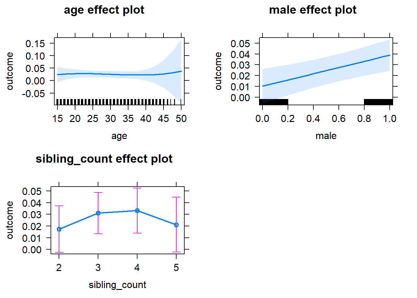
Add Birth Order Linear
Model Summary
tidy(m2_birthorder_linear, conf.int = T, conf.level = 0.995)| effect | group | term | estimate | std.error | statistic | df | p.value | conf.low | conf.high |
|---|---|---|---|---|---|---|---|---|---|
| fixed | NA | (Intercept) | -0.05824 | 0.1336 | -0.4358 | 2615 | 0.663 | -0.4334 | 0.3169 |
| fixed | NA | birth_order | -0.002799 | 0.003184 | -0.879 | 2444 | 0.3795 | -0.01174 | 0.006138 |
| fixed | NA | poly(age, 3, raw = TRUE)1 | 0.007181 | 0.01483 | 0.4841 | 2613 | 0.6284 | -0.03446 | 0.04882 |
| fixed | NA | poly(age, 3, raw = TRUE)2 | -0.0002549 | 0.0005266 | -0.4841 | 2610 | 0.6284 | -0.001733 | 0.001223 |
| fixed | NA | poly(age, 3, raw = TRUE)3 | 0.000002781 | 0.000005989 | 0.4643 | 2607 | 0.6425 | -0.00001403 | 0.00001959 |
| fixed | NA | male | 0.0288 | 0.006223 | 4.627 | 2634 | 0.000003883 | 0.01133 | 0.04627 |
| fixed | NA | sibling_count3 | 0.01512 | 0.008579 | 1.762 | 1965 | 0.07819 | -0.008964 | 0.0392 |
| fixed | NA | sibling_count4 | 0.01867 | 0.009417 | 1.982 | 1859 | 0.04757 | -0.007765 | 0.0451 |
| fixed | NA | sibling_count5 | 0.008339 | 0.01138 | 0.7325 | 1629 | 0.464 | -0.02362 | 0.0403 |
| ran_pars | mother_pidlink | sd__(Intercept) | 0.03594 | NA | NA | NA | NA | NA | NA |
| ran_pars | Residual | sd__Observation | 0.1536 | NA | NA | NA | NA | NA | NA |
Coefficient Plot
plot_birthorder2(m2_birthorder_linear, separate = FALSE)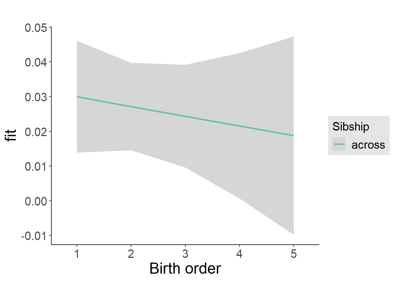
Add Birth Order Factor
Model Summary
m3_birthorder_nonlinear = update(m1_covariates_only, formula = . ~ . + birth_order_nonlinear)
tidy(m3_birthorder_nonlinear, conf.int = T, conf.level = 0.995)| effect | group | term | estimate | std.error | statistic | df | p.value | conf.low | conf.high |
|---|---|---|---|---|---|---|---|---|---|
| fixed | NA | (Intercept) | -0.06563 | 0.1339 | -0.4902 | 2609 | 0.6241 | -0.4415 | 0.3102 |
| fixed | NA | poly(age, 3, raw = TRUE)1 | 0.00784 | 0.01486 | 0.5277 | 2608 | 0.5978 | -0.03387 | 0.04955 |
| fixed | NA | poly(age, 3, raw = TRUE)2 | -0.0002779 | 0.0005274 | -0.5269 | 2606 | 0.5983 | -0.001758 | 0.001203 |
| fixed | NA | poly(age, 3, raw = TRUE)3 | 0.000003031 | 0.000005998 | 0.5054 | 2604 | 0.6133 | -0.0000138 | 0.00001987 |
| fixed | NA | male | 0.02898 | 0.006229 | 4.652 | 2632 | 0.000003448 | 0.01149 | 0.04647 |
| fixed | NA | sibling_count3 | 0.01359 | 0.008719 | 1.558 | 2042 | 0.1193 | -0.01089 | 0.03806 |
| fixed | NA | sibling_count4 | 0.0178 | 0.009548 | 1.865 | 1927 | 0.06239 | -0.008998 | 0.0446 |
| fixed | NA | sibling_count5 | 0.008181 | 0.01157 | 0.7069 | 1690 | 0.4797 | -0.02431 | 0.04067 |
| fixed | NA | birth_order_nonlinear2 | -0.006987 | 0.007448 | -0.9381 | 2175 | 0.3483 | -0.02789 | 0.01392 |
| fixed | NA | birth_order_nonlinear3 | 0.0003167 | 0.009148 | 0.03462 | 2255 | 0.9724 | -0.02536 | 0.026 |
| fixed | NA | birth_order_nonlinear4 | -0.01251 | 0.01253 | -0.9988 | 2340 | 0.318 | -0.04769 | 0.02266 |
| fixed | NA | birth_order_nonlinear5 | -0.01491 | 0.02004 | -0.7439 | 2295 | 0.457 | -0.07116 | 0.04134 |
| ran_pars | mother_pidlink | sd__(Intercept) | 0.03539 | NA | NA | NA | NA | NA | NA |
| ran_pars | Residual | sd__Observation | 0.1537 | NA | NA | NA | NA | NA | NA |
Coefficient Plot
plot_birthorder(m3_birthorder_nonlinear, separate = FALSE)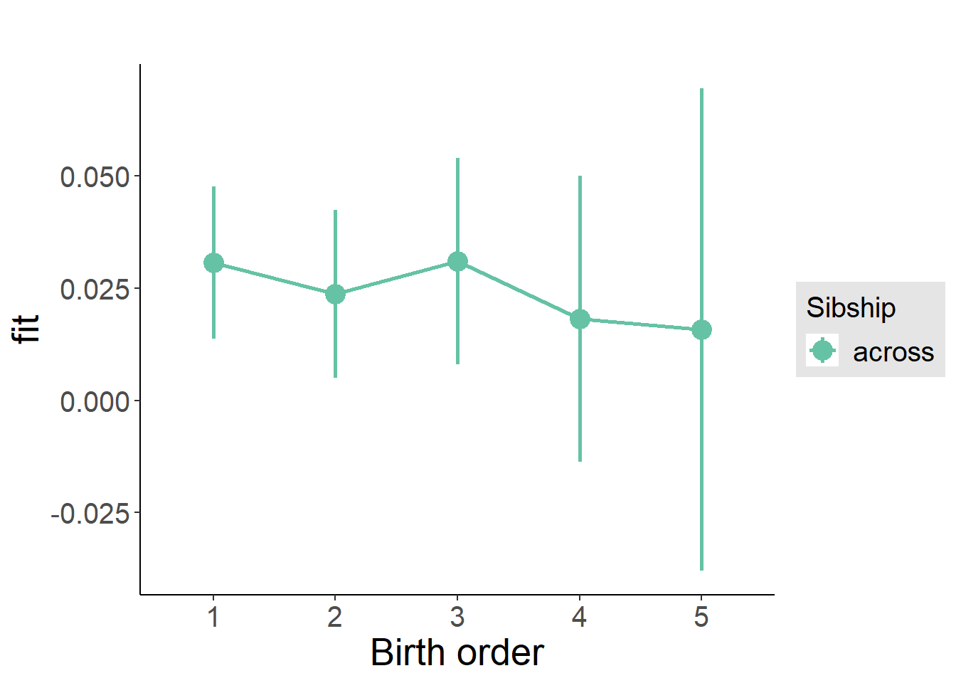
Add Interaction
Model Summary
m4_interaction = update(m3_birthorder_nonlinear, formula = . ~ . - birth_order_nonlinear - sibling_count + count_birth_order)
tidy(m4_interaction, conf.int = T, conf.level = 0.995)| effect | group | term | estimate | std.error | statistic | df | p.value | conf.low | conf.high |
|---|---|---|---|---|---|---|---|---|---|
| fixed | NA | (Intercept) | -0.06923 | 0.1341 | -0.5164 | 2604 | 0.6056 | -0.4455 | 0.3071 |
| fixed | NA | poly(age, 3, raw = TRUE)1 | 0.008296 | 0.01488 | 0.5576 | 2603 | 0.5771 | -0.03347 | 0.05006 |
| fixed | NA | poly(age, 3, raw = TRUE)2 | -0.0002913 | 0.0005282 | -0.5515 | 2601 | 0.5813 | -0.001774 | 0.001191 |
| fixed | NA | poly(age, 3, raw = TRUE)3 | 0.000003154 | 0.000006008 | 0.525 | 2599 | 0.5997 | -0.00001371 | 0.00002002 |
| fixed | NA | male | 0.02916 | 0.006238 | 4.674 | 2625 | 0.000003099 | 0.01165 | 0.04667 |
| fixed | NA | count_birth_order2/2 | -0.01085 | 0.01335 | -0.8131 | 2164 | 0.4163 | -0.04831 | 0.02661 |
| fixed | NA | count_birth_order1/3 | 0.007549 | 0.01124 | 0.6717 | 2627 | 0.5018 | -0.024 | 0.0391 |
| fixed | NA | count_birth_order2/3 | 0.01493 | 0.0125 | 1.195 | 2628 | 0.2324 | -0.02015 | 0.05001 |
| fixed | NA | count_birth_order3/3 | 0.009299 | 0.01347 | 0.6905 | 2624 | 0.4899 | -0.0285 | 0.0471 |
| fixed | NA | count_birth_order1/4 | 0.02208 | 0.01322 | 1.67 | 2628 | 0.09513 | -0.01504 | 0.0592 |
| fixed | NA | count_birth_order2/4 | 0.001129 | 0.01387 | 0.08139 | 2627 | 0.9351 | -0.03782 | 0.04007 |
| fixed | NA | count_birth_order3/4 | 0.01645 | 0.0144 | 1.143 | 2624 | 0.2533 | -0.02397 | 0.05687 |
| fixed | NA | count_birth_order4/4 | 0.007081 | 0.01563 | 0.4531 | 2624 | 0.6505 | -0.03678 | 0.05095 |
| fixed | NA | count_birth_order1/5 | 0.007274 | 0.01734 | 0.4196 | 2628 | 0.6748 | -0.0414 | 0.05594 |
| fixed | NA | count_birth_order2/5 | -0.004573 | 0.01932 | -0.2367 | 2623 | 0.8129 | -0.0588 | 0.04965 |
| fixed | NA | count_birth_order3/5 | 0.01592 | 0.01881 | 0.8464 | 2620 | 0.3974 | -0.03688 | 0.06871 |
| fixed | NA | count_birth_order4/5 | -0.01022 | 0.01809 | -0.5652 | 2618 | 0.572 | -0.061 | 0.04055 |
| fixed | NA | count_birth_order5/5 | -0.008063 | 0.01921 | -0.4197 | 2615 | 0.6747 | -0.06199 | 0.04586 |
| ran_pars | mother_pidlink | sd__(Intercept) | 0.03601 | NA | NA | NA | NA | NA | NA |
| ran_pars | Residual | sd__Observation | 0.1537 | NA | NA | NA | NA | NA | NA |
Coefficient Plot
plot_birthorder(m4_interaction)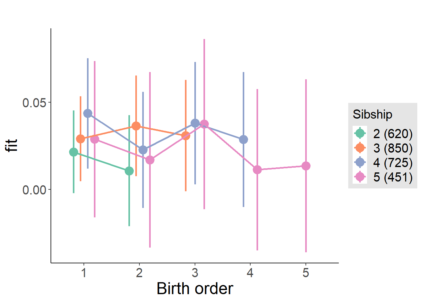
Model Comparison
###### Model 1 - Model 2
anova(m1_covariates_only, m2_birthorder_linear, m3_birthorder_nonlinear, m4_interaction)## refitting model(s) with ML (instead of REML)| Df | AIC | BIC | logLik | deviance | Chisq | Chi Df | Pr(>Chisq) |
|---|---|---|---|---|---|---|---|
| 10 | -2255 | -2197 | 1138 | -2275 | NA | NA | NA |
| 11 | -2254 | -2189 | 1138 | -2276 | 0.769 | 1 | 0.3805 |
| 14 | -2249 | -2167 | 1139 | -2277 | 1.322 | 3 | 0.724 |
| 20 | -2240 | -2123 | 1140 | -2280 | 2.826 | 6 | 0.8303 |
Compare birth order specifications
library(coefplot)
multiplot(outcome_naive_m1, outcome_preg_m1, outcome_uterus_m1, outcome_parental_m1, dodgeHeight = 0.6,
intercept = FALSE)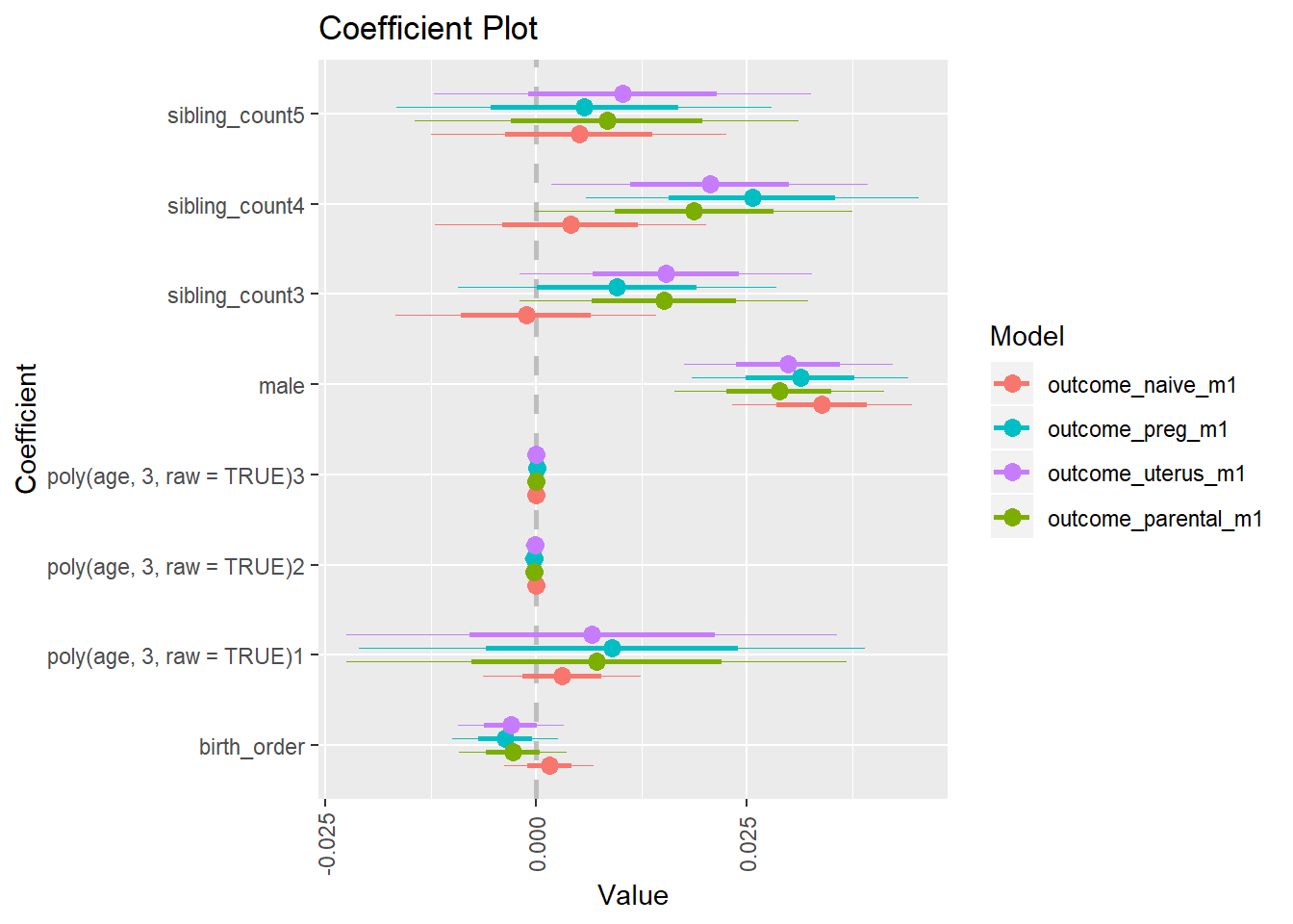
Sector_Social services
birthorder <- birthorder %>% mutate(outcome = `Sector_Social services`)
model = lmer(outcome ~ birth_order + poly(age, 3, raw = TRUE) + male + sibling_count + (1 | mother_pidlink),
data = birthorder)
compare_birthorder_specs(model)Naive birth order
outcome_naive_m1 <- update(m2_birthorder_linear, data = birthorder %>%
mutate(sibling_count = sibling_count_naive_factor,
birth_order_nonlinear = birthorder_naive_factor,
birth_order = birthorder_naive,
count_birth_order = count_birthorder_naive) %>%
filter(sibling_count != "1"))
compare_models_markdown(outcome_naive_m1)Basic Model
Model Summary
m1_covariates_only <- update(m2_birthorder_linear, formula = . ~ . - birth_order)
tidy(m1_covariates_only, conf.int = T, conf.level = 0.995)| effect | group | term | estimate | std.error | statistic | df | p.value | conf.low | conf.high |
|---|---|---|---|---|---|---|---|---|---|
| fixed | NA | (Intercept) | -0.0106 | 0.06663 | -0.1591 | 4184 | 0.8736 | -0.1976 | 0.1764 |
| fixed | NA | poly(age, 3, raw = TRUE)1 | 0.006198 | 0.005921 | 1.047 | 4039 | 0.2952 | -0.01042 | 0.02282 |
| fixed | NA | poly(age, 3, raw = TRUE)2 | -0.0001645 | 0.0001637 | -1.005 | 3885 | 0.3152 | -0.0006241 | 0.0002952 |
| fixed | NA | poly(age, 3, raw = TRUE)3 | 0.000001291 | 0.000001426 | 0.9048 | 3755 | 0.3656 | -0.000002714 | 0.000005295 |
| fixed | NA | male | 0.007712 | 0.006854 | 1.125 | 4623 | 0.2605 | -0.01153 | 0.02695 |
| fixed | NA | sibling_count3 | -0.001109 | 0.009679 | -0.1146 | 3309 | 0.9088 | -0.02828 | 0.02606 |
| fixed | NA | sibling_count4 | -0.006758 | 0.009768 | -0.6918 | 3009 | 0.4891 | -0.03418 | 0.02066 |
| fixed | NA | sibling_count5 | -0.0159 | 0.01014 | -1.568 | 2736 | 0.1171 | -0.04436 | 0.01257 |
| ran_pars | mother_pidlink | sd__(Intercept) | 0.04924 | NA | NA | NA | NA | NA | NA |
| ran_pars | Residual | sd__Observation | 0.2259 | NA | NA | NA | NA | NA | NA |
Coefficient Plot
plot(allEffects(m1_covariates_only, confidence.level = 0.995))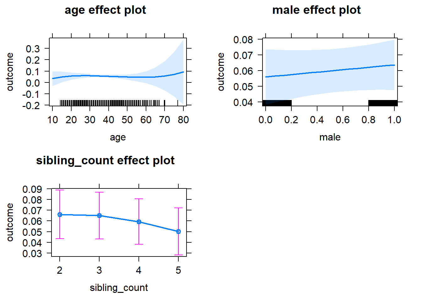
Add Birth Order Linear
Model Summary
tidy(m2_birthorder_linear, conf.int = T, conf.level = 0.995)| effect | group | term | estimate | std.error | statistic | df | p.value | conf.low | conf.high |
|---|---|---|---|---|---|---|---|---|---|
| fixed | NA | (Intercept) | -0.01059 | 0.06665 | -0.159 | 4185 | 0.8737 | -0.1977 | 0.1765 |
| fixed | NA | birth_order | 0.000004172 | 0.003395 | 0.001229 | 4186 | 0.999 | -0.009524 | 0.009533 |
| fixed | NA | poly(age, 3, raw = TRUE)1 | 0.006197 | 0.005944 | 1.043 | 4041 | 0.2972 | -0.01049 | 0.02288 |
| fixed | NA | poly(age, 3, raw = TRUE)2 | -0.0001645 | 0.0001643 | -1.001 | 3878 | 0.3168 | -0.0006256 | 0.0002967 |
| fixed | NA | poly(age, 3, raw = TRUE)3 | 0.00000129 | 0.000001429 | 0.9028 | 3748 | 0.3667 | -0.000002722 | 0.000005302 |
| fixed | NA | male | 0.007713 | 0.006854 | 1.125 | 4622 | 0.2606 | -0.01153 | 0.02695 |
| fixed | NA | sibling_count3 | -0.001111 | 0.009766 | -0.1137 | 3399 | 0.9095 | -0.02852 | 0.0263 |
| fixed | NA | sibling_count4 | -0.006761 | 0.01016 | -0.6656 | 3384 | 0.5057 | -0.03527 | 0.02175 |
| fixed | NA | sibling_count5 | -0.0159 | 0.01105 | -1.439 | 3486 | 0.1502 | -0.04692 | 0.01511 |
| ran_pars | mother_pidlink | sd__(Intercept) | 0.0492 | NA | NA | NA | NA | NA | NA |
| ran_pars | Residual | sd__Observation | 0.226 | NA | NA | NA | NA | NA | NA |
Coefficient Plot
plot_birthorder2(m2_birthorder_linear, separate = FALSE)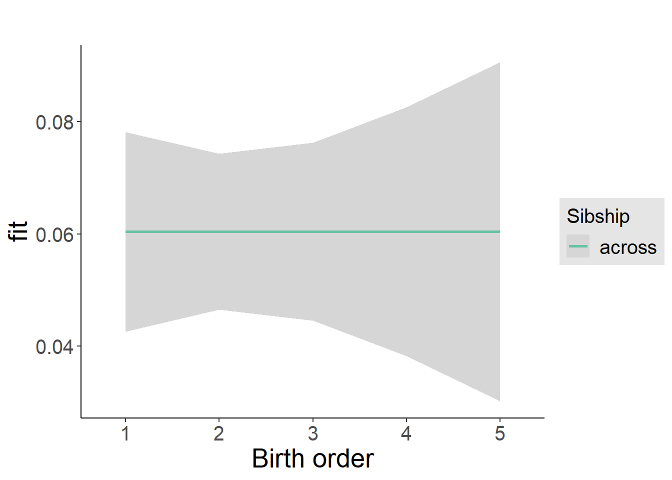
Add Birth Order Factor
Model Summary
m3_birthorder_nonlinear = update(m1_covariates_only, formula = . ~ . + birth_order_nonlinear)
tidy(m3_birthorder_nonlinear, conf.int = T, conf.level = 0.995)| effect | group | term | estimate | std.error | statistic | df | p.value | conf.low | conf.high |
|---|---|---|---|---|---|---|---|---|---|
| fixed | NA | (Intercept) | -0.01191 | 0.06687 | -0.1781 | 4191 | 0.8586 | -0.1996 | 0.1758 |
| fixed | NA | poly(age, 3, raw = TRUE)1 | 0.006289 | 0.005947 | 1.057 | 4036 | 0.2904 | -0.0104 | 0.02298 |
| fixed | NA | poly(age, 3, raw = TRUE)2 | -0.000166 | 0.0001644 | -1.01 | 3869 | 0.3127 | -0.0006274 | 0.0002954 |
| fixed | NA | poly(age, 3, raw = TRUE)3 | 0.000001294 | 0.000001431 | 0.9045 | 3733 | 0.3658 | -0.000002722 | 0.00000531 |
| fixed | NA | male | 0.007815 | 0.006858 | 1.139 | 4619 | 0.2546 | -0.01144 | 0.02707 |
| fixed | NA | sibling_count3 | -0.0002059 | 0.009947 | -0.0207 | 3561 | 0.9835 | -0.02813 | 0.02772 |
| fixed | NA | sibling_count4 | -0.004984 | 0.01036 | -0.4813 | 3562 | 0.6304 | -0.03406 | 0.02409 |
| fixed | NA | sibling_count5 | -0.01664 | 0.01117 | -1.49 | 3589 | 0.1364 | -0.04799 | 0.01471 |
| fixed | NA | birth_order_nonlinear2 | -0.0002603 | 0.008193 | -0.03178 | 4061 | 0.9747 | -0.02326 | 0.02274 |
| fixed | NA | birth_order_nonlinear3 | -0.003861 | 0.01039 | -0.3717 | 4044 | 0.7101 | -0.03302 | 0.0253 |
| fixed | NA | birth_order_nonlinear4 | -0.005168 | 0.01357 | -0.3808 | 4028 | 0.7034 | -0.04327 | 0.03293 |
| fixed | NA | birth_order_nonlinear5 | 0.01357 | 0.01958 | 0.6931 | 4104 | 0.4883 | -0.04139 | 0.06853 |
| ran_pars | mother_pidlink | sd__(Intercept) | 0.04904 | NA | NA | NA | NA | NA | NA |
| ran_pars | Residual | sd__Observation | 0.2261 | NA | NA | NA | NA | NA | NA |
Coefficient Plot
plot_birthorder(m3_birthorder_nonlinear, separate = FALSE)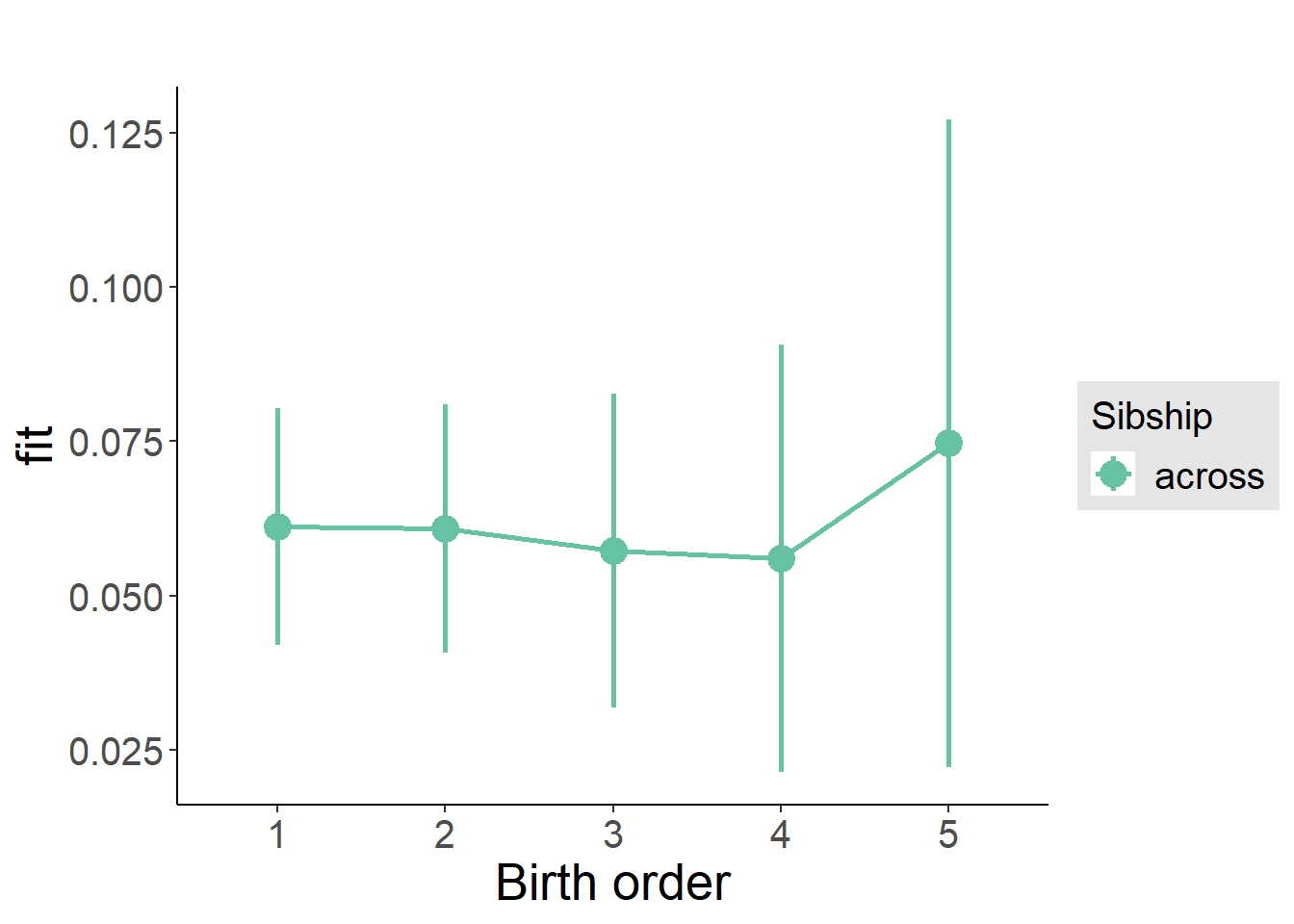
Add Interaction
Model Summary
m4_interaction = update(m3_birthorder_nonlinear, formula = . ~ . - birth_order_nonlinear - sibling_count + count_birth_order)
tidy(m4_interaction, conf.int = T, conf.level = 0.995)| effect | group | term | estimate | std.error | statistic | df | p.value | conf.low | conf.high |
|---|---|---|---|---|---|---|---|---|---|
| fixed | NA | (Intercept) | -0.01779 | 0.06699 | -0.2656 | 4197 | 0.7906 | -0.2058 | 0.1703 |
| fixed | NA | poly(age, 3, raw = TRUE)1 | 0.006093 | 0.005953 | 1.023 | 4035 | 0.3062 | -0.01062 | 0.0228 |
| fixed | NA | poly(age, 3, raw = TRUE)2 | -0.0001639 | 0.0001645 | -0.9966 | 3868 | 0.319 | -0.0006257 | 0.0002978 |
| fixed | NA | poly(age, 3, raw = TRUE)3 | 0.000001307 | 0.000001431 | 0.9128 | 3731 | 0.3614 | -0.000002711 | 0.000005324 |
| fixed | NA | male | 0.00761 | 0.006859 | 1.109 | 4611 | 0.2673 | -0.01164 | 0.02686 |
| fixed | NA | count_birth_order2/2 | 0.02447 | 0.01394 | 1.755 | 3949 | 0.07939 | -0.01467 | 0.06361 |
| fixed | NA | count_birth_order1/3 | 0.01066 | 0.01326 | 0.8039 | 4622 | 0.4215 | -0.02656 | 0.04787 |
| fixed | NA | count_birth_order2/3 | 0.002391 | 0.01476 | 0.162 | 4624 | 0.8713 | -0.03904 | 0.04383 |
| fixed | NA | count_birth_order3/3 | 0.01103 | 0.01624 | 0.6791 | 4625 | 0.4971 | -0.03456 | 0.05662 |
| fixed | NA | count_birth_order1/4 | 0.01603 | 0.01461 | 1.097 | 4625 | 0.2727 | -0.02498 | 0.05703 |
| fixed | NA | count_birth_order2/4 | 0.00377 | 0.01567 | 0.2405 | 4624 | 0.8099 | -0.04023 | 0.04777 |
| fixed | NA | count_birth_order3/4 | -0.01053 | 0.01654 | -0.6363 | 4625 | 0.5246 | -0.05697 | 0.03591 |
| fixed | NA | count_birth_order4/4 | -0.006882 | 0.01784 | -0.3858 | 4625 | 0.6997 | -0.05696 | 0.04319 |
| fixed | NA | count_birth_order1/5 | -0.002279 | 0.01648 | -0.1383 | 4625 | 0.89 | -0.04854 | 0.04399 |
| fixed | NA | count_birth_order2/5 | -0.02511 | 0.01752 | -1.433 | 4624 | 0.1518 | -0.07428 | 0.02406 |
| fixed | NA | count_birth_order3/5 | -0.004062 | 0.01843 | -0.2204 | 4624 | 0.8256 | -0.0558 | 0.04767 |
| fixed | NA | count_birth_order4/5 | -0.004579 | 0.01948 | -0.2351 | 4622 | 0.8141 | -0.05925 | 0.05009 |
| fixed | NA | count_birth_order5/5 | 0.006435 | 0.01952 | 0.3296 | 4625 | 0.7417 | -0.04836 | 0.06123 |
| ran_pars | mother_pidlink | sd__(Intercept) | 0.04993 | NA | NA | NA | NA | NA | NA |
| ran_pars | Residual | sd__Observation | 0.2258 | NA | NA | NA | NA | NA | NA |
Coefficient Plot
plot_birthorder(m4_interaction)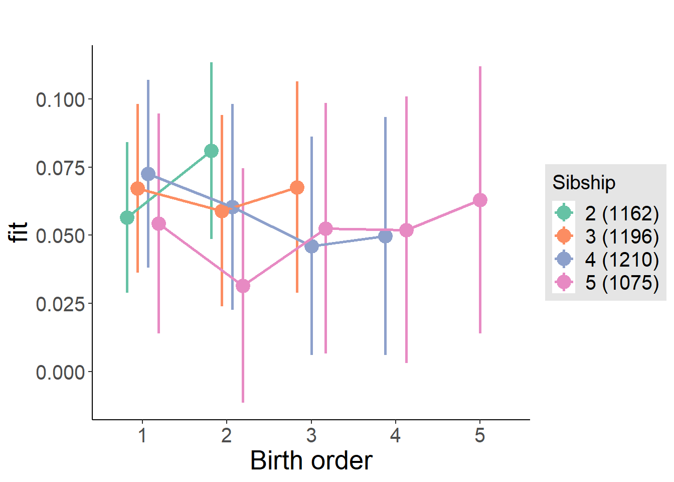
Model Comparison
###### Model 1 - Model 2
anova(m1_covariates_only, m2_birthorder_linear, m3_birthorder_nonlinear, m4_interaction)## refitting model(s) with ML (instead of REML)| Df | AIC | BIC | logLik | deviance | Chisq | Chi Df | Pr(>Chisq) |
|---|---|---|---|---|---|---|---|
| 10 | -413.3 | -348.9 | 216.6 | -433.3 | NA | NA | NA |
| 11 | -411.3 | -340.4 | 216.6 | -433.3 | 0.000003217 | 1 | 0.9986 |
| 14 | -406.2 | -316 | 217.1 | -434.2 | 0.9419 | 3 | 0.8153 |
| 20 | -401.6 | -272.8 | 220.8 | -441.6 | 7.4 | 6 | 0.2854 |
Maternal birth order
outcome_uterus_m1 <- update(m2_birthorder_linear, data = birthorder %>%
mutate(sibling_count = sibling_count_uterus_alive_factor,
birth_order_nonlinear = birthorder_uterus_alive_factor,
birth_order = birthorder_uterus_alive,
count_birth_order = count_birthorder_uterus_alive) %>%
filter(sibling_count != "1"))
compare_models_markdown(outcome_uterus_m1)Basic Model
Model Summary
m1_covariates_only <- update(m2_birthorder_linear, formula = . ~ . - birth_order)
tidy(m1_covariates_only, conf.int = T, conf.level = 0.995)| effect | group | term | estimate | std.error | statistic | df | p.value | conf.low | conf.high |
|---|---|---|---|---|---|---|---|---|---|
| fixed | NA | (Intercept) | -0.2246 | 0.1959 | -1.147 | 2616 | 0.2515 | -0.7745 | 0.3252 |
| fixed | NA | poly(age, 3, raw = TRUE)1 | 0.02944 | 0.02168 | 1.358 | 2615 | 0.1745 | -0.03141 | 0.09029 |
| fixed | NA | poly(age, 3, raw = TRUE)2 | -0.0009834 | 0.0007678 | -1.281 | 2612 | 0.2003 | -0.003139 | 0.001172 |
| fixed | NA | poly(age, 3, raw = TRUE)3 | 0.00001074 | 0.000008708 | 1.233 | 2609 | 0.2176 | -0.00001371 | 0.00003518 |
| fixed | NA | male | 0.009916 | 0.009229 | 1.074 | 2634 | 0.2827 | -0.01599 | 0.03582 |
| fixed | NA | sibling_count3 | -0.006129 | 0.01268 | -0.4833 | 2173 | 0.6289 | -0.04172 | 0.02947 |
| fixed | NA | sibling_count4 | -0.01875 | 0.01309 | -1.433 | 1973 | 0.152 | -0.05549 | 0.01798 |
| fixed | NA | sibling_count5 | -0.002224 | 0.01452 | -0.1531 | 1683 | 0.8783 | -0.043 | 0.03855 |
| ran_pars | mother_pidlink | sd__(Intercept) | 0.02621 | NA | NA | NA | NA | NA | NA |
| ran_pars | Residual | sd__Observation | 0.2321 | NA | NA | NA | NA | NA | NA |
Coefficient Plot
plot(allEffects(m1_covariates_only, confidence.level = 0.995))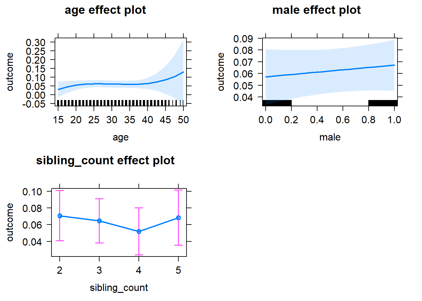
Add Birth Order Linear
Model Summary
tidy(m2_birthorder_linear, conf.int = T, conf.level = 0.995)| effect | group | term | estimate | std.error | statistic | df | p.value | conf.low | conf.high |
|---|---|---|---|---|---|---|---|---|---|
| fixed | NA | (Intercept) | -0.2243 | 0.1959 | -1.145 | 2616 | 0.2524 | -0.7742 | 0.3256 |
| fixed | NA | birth_order | -0.001622 | 0.004676 | -0.3468 | 2550 | 0.7287 | -0.01475 | 0.0115 |
| fixed | NA | poly(age, 3, raw = TRUE)1 | 0.02959 | 0.02168 | 1.364 | 2613 | 0.1725 | -0.03128 | 0.09046 |
| fixed | NA | poly(age, 3, raw = TRUE)2 | -0.0009858 | 0.0007679 | -1.284 | 2611 | 0.1994 | -0.003141 | 0.00117 |
| fixed | NA | poly(age, 3, raw = TRUE)3 | 0.00001073 | 0.00000871 | 1.231 | 2608 | 0.2183 | -0.00001372 | 0.00003517 |
| fixed | NA | male | 0.009911 | 0.009231 | 1.074 | 2633 | 0.2831 | -0.016 | 0.03582 |
| fixed | NA | sibling_count3 | -0.005364 | 0.01287 | -0.4167 | 2202 | 0.677 | -0.0415 | 0.03077 |
| fixed | NA | sibling_count4 | -0.0171 | 0.01393 | -1.228 | 2098 | 0.2197 | -0.0562 | 0.022 |
| fixed | NA | sibling_count5 | 0.0005365 | 0.01657 | 0.03239 | 2010 | 0.9742 | -0.04596 | 0.04704 |
| ran_pars | mother_pidlink | sd__(Intercept) | 0.02621 | NA | NA | NA | NA | NA | NA |
| ran_pars | Residual | sd__Observation | 0.2322 | NA | NA | NA | NA | NA | NA |
Coefficient Plot
plot_birthorder2(m2_birthorder_linear, separate = FALSE)
Add Birth Order Factor
Model Summary
m3_birthorder_nonlinear = update(m1_covariates_only, formula = . ~ . + birth_order_nonlinear)
tidy(m3_birthorder_nonlinear, conf.int = T, conf.level = 0.995)| effect | group | term | estimate | std.error | statistic | df | p.value | conf.low | conf.high |
|---|---|---|---|---|---|---|---|---|---|
| fixed | NA | (Intercept) | -0.2206 | 0.1963 | -1.124 | 2612 | 0.2611 | -0.7716 | 0.3303 |
| fixed | NA | poly(age, 3, raw = TRUE)1 | 0.02947 | 0.02172 | 1.357 | 2610 | 0.1748 | -0.03148 | 0.09043 |
| fixed | NA | poly(age, 3, raw = TRUE)2 | -0.0009792 | 0.000769 | -1.273 | 2608 | 0.203 | -0.003138 | 0.001179 |
| fixed | NA | poly(age, 3, raw = TRUE)3 | 0.00001063 | 0.000008721 | 1.219 | 2606 | 0.2228 | -0.00001385 | 0.00003512 |
| fixed | NA | male | 0.009571 | 0.009236 | 1.036 | 2630 | 0.3002 | -0.01636 | 0.0355 |
| fixed | NA | sibling_count3 | -0.006408 | 0.01308 | -0.4899 | 2255 | 0.6243 | -0.04313 | 0.03031 |
| fixed | NA | sibling_count4 | -0.02085 | 0.01413 | -1.476 | 2150 | 0.1402 | -0.06052 | 0.01882 |
| fixed | NA | sibling_count5 | -0.0005539 | 0.01679 | -0.03299 | 2050 | 0.9737 | -0.04768 | 0.04657 |
| fixed | NA | birth_order_nonlinear2 | -0.01649 | 0.01121 | -1.471 | 2373 | 0.1414 | -0.04795 | 0.01497 |
| fixed | NA | birth_order_nonlinear3 | -0.00008333 | 0.01365 | -0.006104 | 2427 | 0.9951 | -0.03841 | 0.03824 |
| fixed | NA | birth_order_nonlinear4 | 0.005212 | 0.01816 | 0.2871 | 2491 | 0.7741 | -0.04576 | 0.05618 |
| fixed | NA | birth_order_nonlinear5 | -0.02791 | 0.02816 | -0.9913 | 2456 | 0.3216 | -0.107 | 0.05113 |
| ran_pars | mother_pidlink | sd__(Intercept) | 0.0282 | NA | NA | NA | NA | NA | NA |
| ran_pars | Residual | sd__Observation | 0.2319 | NA | NA | NA | NA | NA | NA |
Coefficient Plot
plot_birthorder(m3_birthorder_nonlinear, separate = FALSE)
Add Interaction
Model Summary
m4_interaction = update(m3_birthorder_nonlinear, formula = . ~ . - birth_order_nonlinear - sibling_count + count_birth_order)
tidy(m4_interaction, conf.int = T, conf.level = 0.995)| effect | group | term | estimate | std.error | statistic | df | p.value | conf.low | conf.high |
|---|---|---|---|---|---|---|---|---|---|
| fixed | NA | (Intercept) | -0.2203 | 0.1965 | -1.121 | 2606 | 0.2623 | -0.7718 | 0.3312 |
| fixed | NA | poly(age, 3, raw = TRUE)1 | 0.02899 | 0.02174 | 1.334 | 2604 | 0.1825 | -0.03203 | 0.09 |
| fixed | NA | poly(age, 3, raw = TRUE)2 | -0.0009596 | 0.0007699 | -1.246 | 2602 | 0.2127 | -0.003121 | 0.001201 |
| fixed | NA | poly(age, 3, raw = TRUE)3 | 0.00001037 | 0.000008732 | 1.188 | 2599 | 0.235 | -0.00001414 | 0.00003489 |
| fixed | NA | male | 0.009276 | 0.009252 | 1.003 | 2624 | 0.3161 | -0.01669 | 0.03525 |
| fixed | NA | count_birth_order2/2 | -0.004822 | 0.02045 | -0.2358 | 2349 | 0.8136 | -0.06221 | 0.05257 |
| fixed | NA | count_birth_order1/3 | -0.004718 | 0.01694 | -0.2785 | 2624 | 0.7806 | -0.05227 | 0.04284 |
| fixed | NA | count_birth_order2/3 | -0.03044 | 0.01883 | -1.616 | 2624 | 0.1062 | -0.0833 | 0.02243 |
| fixed | NA | count_birth_order3/3 | 0.01643 | 0.02053 | 0.8003 | 2623 | 0.4236 | -0.0412 | 0.07406 |
| fixed | NA | count_birth_order1/4 | -0.01174 | 0.01949 | -0.6022 | 2624 | 0.5471 | -0.06645 | 0.04297 |
| fixed | NA | count_birth_order2/4 | -0.02657 | 0.02064 | -1.288 | 2624 | 0.198 | -0.08451 | 0.03136 |
| fixed | NA | count_birth_order3/4 | -0.03235 | 0.02141 | -1.511 | 2624 | 0.1309 | -0.09245 | 0.02775 |
| fixed | NA | count_birth_order4/4 | -0.01096 | 0.02289 | -0.4786 | 2624 | 0.6322 | -0.07522 | 0.0533 |
| fixed | NA | count_birth_order1/5 | 0.01401 | 0.02574 | 0.5445 | 2623 | 0.5862 | -0.05823 | 0.08626 |
| fixed | NA | count_birth_order2/5 | -0.01272 | 0.02771 | -0.459 | 2624 | 0.6463 | -0.09049 | 0.06506 |
| fixed | NA | count_birth_order3/5 | -0.007082 | 0.02632 | -0.2691 | 2624 | 0.7879 | -0.08095 | 0.06679 |
| fixed | NA | count_birth_order4/5 | 0.007286 | 0.02565 | 0.284 | 2623 | 0.7764 | -0.06472 | 0.0793 |
| fixed | NA | count_birth_order5/5 | -0.02465 | 0.02699 | -0.9132 | 2622 | 0.3612 | -0.1004 | 0.05112 |
| ran_pars | mother_pidlink | sd__(Intercept) | 0.02655 | NA | NA | NA | NA | NA | NA |
| ran_pars | Residual | sd__Observation | 0.2322 | NA | NA | NA | NA | NA | NA |
Coefficient Plot
plot_birthorder(m4_interaction)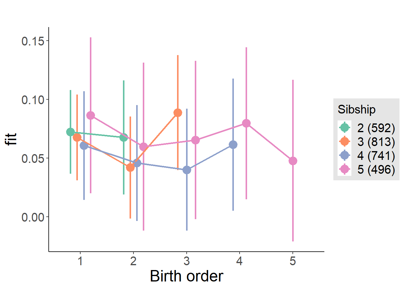
Model Comparison
###### Model 1 - Model 2
anova(m1_covariates_only, m2_birthorder_linear, m3_birthorder_nonlinear, m4_interaction)## refitting model(s) with ML (instead of REML)| Df | AIC | BIC | logLik | deviance | Chisq | Chi Df | Pr(>Chisq) |
|---|---|---|---|---|---|---|---|
| 10 | -174 | -115.2 | 97 | -194 | NA | NA | NA |
| 11 | -172.1 | -107.4 | 97.06 | -194.1 | 0.1205 | 1 | 0.7285 |
| 14 | -169.8 | -87.46 | 98.89 | -197.8 | 3.655 | 3 | 0.3012 |
| 20 | -161.5 | -43.91 | 100.7 | -201.5 | 3.72 | 6 | 0.7145 |
Maternal pregnancy order
outcome_preg_m1 <- update(m2_birthorder_linear, data = birthorder %>%
mutate(sibling_count = sibling_count_uterus_preg_factor,
birth_order_nonlinear = birthorder_uterus_preg_factor,
birth_order = birthorder_uterus_preg,
count_birth_order = count_birthorder_uterus_preg
) %>%
filter(sibling_count != "1"))
compare_models_markdown(outcome_preg_m1)Basic Model
Model Summary
m1_covariates_only <- update(m2_birthorder_linear, formula = . ~ . - birth_order)
tidy(m1_covariates_only, conf.int = T, conf.level = 0.995)| effect | group | term | estimate | std.error | statistic | df | p.value | conf.low | conf.high |
|---|---|---|---|---|---|---|---|---|---|
| fixed | NA | (Intercept) | -0.2967 | 0.2013 | -1.474 | 2409 | 0.1406 | -0.8616 | 0.2683 |
| fixed | NA | poly(age, 3, raw = TRUE)1 | 0.0381 | 0.02229 | 1.709 | 2408 | 0.08752 | -0.02447 | 0.1007 |
| fixed | NA | poly(age, 3, raw = TRUE)2 | -0.001307 | 0.0007895 | -1.656 | 2406 | 0.09794 | -0.003523 | 0.000909 |
| fixed | NA | poly(age, 3, raw = TRUE)3 | 0.00001457 | 0.000008956 | 1.627 | 2404 | 0.1039 | -0.00001057 | 0.00003971 |
| fixed | NA | male | 0.01207 | 0.009549 | 1.264 | 2419 | 0.2062 | -0.01473 | 0.03888 |
| fixed | NA | sibling_count3 | -0.009292 | 0.01384 | -0.6713 | 2014 | 0.5021 | -0.04815 | 0.02956 |
| fixed | NA | sibling_count4 | -0.01757 | 0.01399 | -1.256 | 1899 | 0.2094 | -0.05683 | 0.0217 |
| fixed | NA | sibling_count5 | -0.01353 | 0.01472 | -0.919 | 1729 | 0.3582 | -0.05485 | 0.02779 |
| ran_pars | mother_pidlink | sd__(Intercept) | 0.04002 | NA | NA | NA | NA | NA | NA |
| ran_pars | Residual | sd__Observation | 0.2281 | NA | NA | NA | NA | NA | NA |
Coefficient Plot
plot(allEffects(m1_covariates_only, confidence.level = 0.995))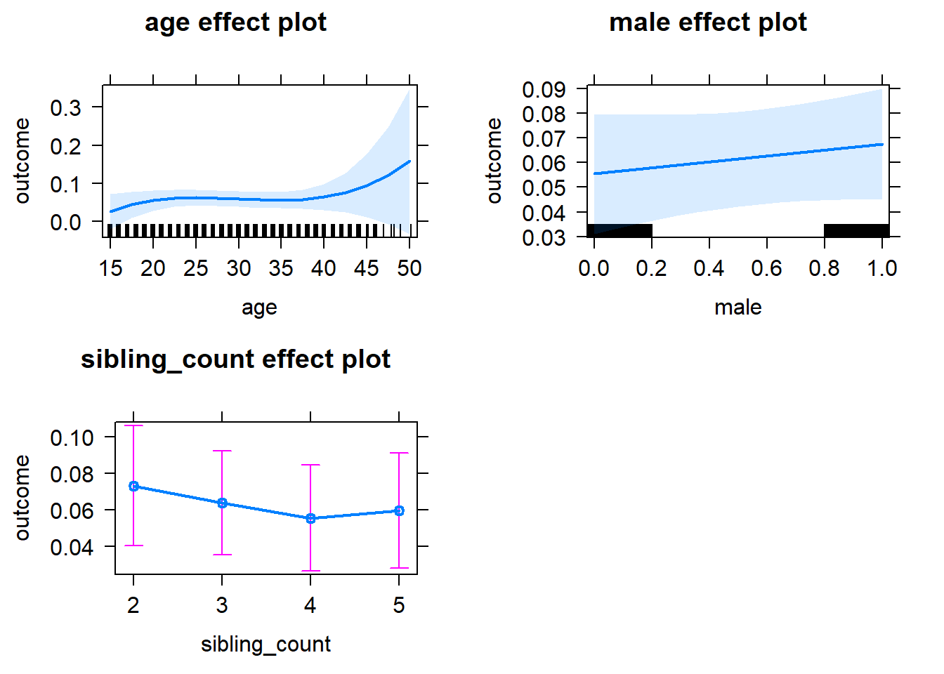
Add Birth Order Linear
Model Summary
tidy(m2_birthorder_linear, conf.int = T, conf.level = 0.995)| effect | group | term | estimate | std.error | statistic | df | p.value | conf.low | conf.high |
|---|---|---|---|---|---|---|---|---|---|
| fixed | NA | (Intercept) | -0.295 | 0.2013 | -1.465 | 2408 | 0.143 | -0.8601 | 0.2701 |
| fixed | NA | birth_order | -0.002264 | 0.004692 | -0.4826 | 2370 | 0.6294 | -0.01543 | 0.01091 |
| fixed | NA | poly(age, 3, raw = TRUE)1 | 0.0382 | 0.02229 | 1.714 | 2407 | 0.08672 | -0.02437 | 0.1008 |
| fixed | NA | poly(age, 3, raw = TRUE)2 | -0.001308 | 0.0007896 | -1.656 | 2405 | 0.09781 | -0.003524 | 0.0009087 |
| fixed | NA | poly(age, 3, raw = TRUE)3 | 0.00001453 | 0.000008958 | 1.622 | 2403 | 0.105 | -0.00001062 | 0.00003967 |
| fixed | NA | male | 0.01201 | 0.009552 | 1.257 | 2418 | 0.2088 | -0.0148 | 0.03882 |
| fixed | NA | sibling_count3 | -0.008216 | 0.01402 | -0.5859 | 2031 | 0.558 | -0.04758 | 0.03115 |
| fixed | NA | sibling_count4 | -0.01544 | 0.01467 | -1.052 | 1973 | 0.2928 | -0.05662 | 0.02574 |
| fixed | NA | sibling_count5 | -0.009919 | 0.01651 | -0.6006 | 1953 | 0.5482 | -0.05627 | 0.03644 |
| ran_pars | mother_pidlink | sd__(Intercept) | 0.03999 | NA | NA | NA | NA | NA | NA |
| ran_pars | Residual | sd__Observation | 0.2282 | NA | NA | NA | NA | NA | NA |
Coefficient Plot
plot_birthorder2(m2_birthorder_linear, separate = FALSE)
Add Birth Order Factor
Model Summary
m3_birthorder_nonlinear = update(m1_covariates_only, formula = . ~ . + birth_order_nonlinear)
tidy(m3_birthorder_nonlinear, conf.int = T, conf.level = 0.995)| effect | group | term | estimate | std.error | statistic | df | p.value | conf.low | conf.high |
|---|---|---|---|---|---|---|---|---|---|
| fixed | NA | (Intercept) | -0.3003 | 0.2018 | -1.488 | 2403 | 0.1369 | -0.8669 | 0.2662 |
| fixed | NA | poly(age, 3, raw = TRUE)1 | 0.03889 | 0.02235 | 1.741 | 2402 | 0.08189 | -0.02383 | 0.1016 |
| fixed | NA | poly(age, 3, raw = TRUE)2 | -0.001329 | 0.0007915 | -1.679 | 2401 | 0.09323 | -0.003551 | 0.0008926 |
| fixed | NA | poly(age, 3, raw = TRUE)3 | 0.00001474 | 0.000008978 | 1.641 | 2399 | 0.1008 | -0.00001046 | 0.00003994 |
| fixed | NA | male | 0.01188 | 0.00956 | 1.243 | 2415 | 0.2141 | -0.01496 | 0.03871 |
| fixed | NA | sibling_count3 | -0.009676 | 0.01423 | -0.6798 | 2073 | 0.4967 | -0.04963 | 0.03028 |
| fixed | NA | sibling_count4 | -0.0179 | 0.01487 | -1.204 | 2013 | 0.2288 | -0.05962 | 0.02383 |
| fixed | NA | sibling_count5 | -0.01075 | 0.01663 | -0.6465 | 1975 | 0.518 | -0.05743 | 0.03593 |
| fixed | NA | birth_order_nonlinear2 | -0.01379 | 0.0115 | -1.199 | 2167 | 0.2305 | -0.04606 | 0.01848 |
| fixed | NA | birth_order_nonlinear3 | 0.001024 | 0.01415 | 0.07239 | 2253 | 0.9423 | -0.03869 | 0.04074 |
| fixed | NA | birth_order_nonlinear4 | -0.003478 | 0.01865 | -0.1865 | 2311 | 0.8521 | -0.05583 | 0.04888 |
| fixed | NA | birth_order_nonlinear5 | -0.02216 | 0.0268 | -0.8266 | 2257 | 0.4086 | -0.0974 | 0.05309 |
| ran_pars | mother_pidlink | sd__(Intercept) | 0.04086 | NA | NA | NA | NA | NA | NA |
| ran_pars | Residual | sd__Observation | 0.2281 | NA | NA | NA | NA | NA | NA |
Coefficient Plot
plot_birthorder(m3_birthorder_nonlinear, separate = FALSE)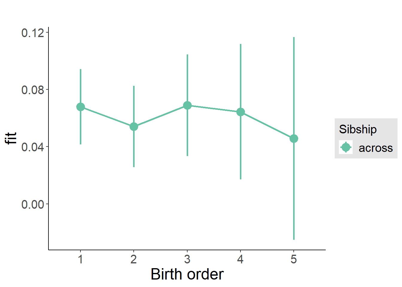
Add Interaction
Model Summary
m4_interaction = update(m3_birthorder_nonlinear, formula = . ~ . - birth_order_nonlinear - sibling_count + count_birth_order)
tidy(m4_interaction, conf.int = T, conf.level = 0.995)| effect | group | term | estimate | std.error | statistic | df | p.value | conf.low | conf.high |
|---|---|---|---|---|---|---|---|---|---|
| fixed | NA | (Intercept) | -0.2995 | 0.2022 | -1.481 | 2397 | 0.1387 | -0.8671 | 0.2681 |
| fixed | NA | poly(age, 3, raw = TRUE)1 | 0.03831 | 0.02239 | 1.711 | 2396 | 0.08712 | -0.02453 | 0.1012 |
| fixed | NA | poly(age, 3, raw = TRUE)2 | -0.001308 | 0.0007929 | -1.65 | 2395 | 0.09917 | -0.003534 | 0.0009178 |
| fixed | NA | poly(age, 3, raw = TRUE)3 | 0.00001448 | 0.000008994 | 1.609 | 2392 | 0.1076 | -0.00001077 | 0.00003972 |
| fixed | NA | male | 0.01165 | 0.009586 | 1.215 | 2409 | 0.2245 | -0.01526 | 0.03856 |
| fixed | NA | count_birth_order2/2 | -0.00005427 | 0.02217 | -0.002448 | 2189 | 0.998 | -0.06229 | 0.06218 |
| fixed | NA | count_birth_order1/3 | -0.009228 | 0.0186 | -0.4963 | 2409 | 0.6198 | -0.06143 | 0.04297 |
| fixed | NA | count_birth_order2/3 | -0.02607 | 0.02024 | -1.288 | 2409 | 0.1979 | -0.08288 | 0.03074 |
| fixed | NA | count_birth_order3/3 | 0.01425 | 0.02245 | 0.635 | 2408 | 0.5255 | -0.04875 | 0.07726 |
| fixed | NA | count_birth_order1/4 | -0.003288 | 0.02024 | -0.1624 | 2409 | 0.871 | -0.06011 | 0.05353 |
| fixed | NA | count_birth_order2/4 | -0.03242 | 0.0213 | -1.522 | 2409 | 0.1281 | -0.09222 | 0.02737 |
| fixed | NA | count_birth_order3/4 | -0.02672 | 0.02306 | -1.159 | 2408 | 0.2467 | -0.09144 | 0.038 |
| fixed | NA | count_birth_order4/4 | -0.008554 | 0.02502 | -0.342 | 2408 | 0.7324 | -0.07877 | 0.06166 |
| fixed | NA | count_birth_order1/5 | -0.001764 | 0.02451 | -0.07195 | 2409 | 0.9426 | -0.07057 | 0.06704 |
| fixed | NA | count_birth_order2/5 | -0.009901 | 0.0251 | -0.3945 | 2409 | 0.6932 | -0.08034 | 0.06054 |
| fixed | NA | count_birth_order3/5 | -0.01172 | 0.0258 | -0.4541 | 2408 | 0.6498 | -0.08415 | 0.06072 |
| fixed | NA | count_birth_order4/5 | -0.01896 | 0.02622 | -0.7231 | 2407 | 0.4697 | -0.09255 | 0.05464 |
| fixed | NA | count_birth_order5/5 | -0.02826 | 0.02662 | -1.061 | 2405 | 0.2886 | -0.103 | 0.04648 |
| ran_pars | mother_pidlink | sd__(Intercept) | 0.03943 | NA | NA | NA | NA | NA | NA |
| ran_pars | Residual | sd__Observation | 0.2284 | NA | NA | NA | NA | NA | NA |
Coefficient Plot
plot_birthorder(m4_interaction)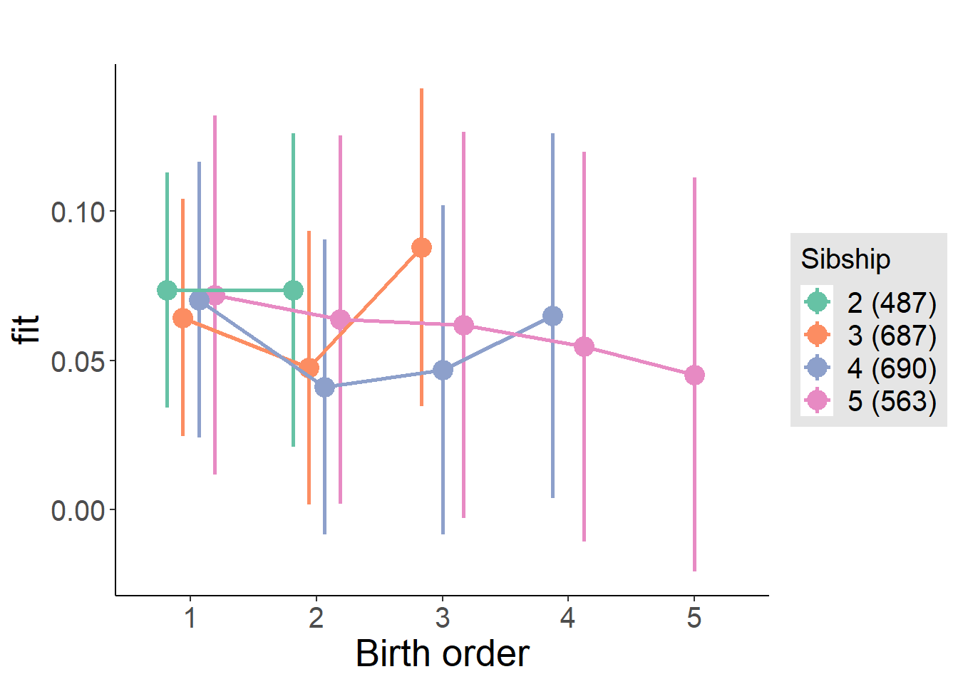
Model Comparison
###### Model 1 - Model 2
anova(m1_covariates_only, m2_birthorder_linear, m3_birthorder_nonlinear, m4_interaction)## refitting model(s) with ML (instead of REML)| Df | AIC | BIC | logLik | deviance | Chisq | Chi Df | Pr(>Chisq) |
|---|---|---|---|---|---|---|---|
| 10 | -201.1 | -143.2 | 110.6 | -221.1 | NA | NA | NA |
| 11 | -199.4 | -135.6 | 110.7 | -221.4 | 0.2337 | 1 | 0.6288 |
| 14 | -195.4 | -114.2 | 111.7 | -223.4 | 2.013 | 3 | 0.5697 |
| 20 | -186.9 | -71.01 | 113.4 | -226.9 | 3.526 | 6 | 0.7405 |
Parental full sibling order
outcome_parental_m1 <- update(m2_birthorder_linear, data = birthorder %>%
mutate(sibling_count = sibling_count_genes_factor,
birth_order_nonlinear = birthorder_genes_factor,
birth_order = birthorder_genes,
count_birth_order = count_birthorder_genes
) %>%
filter(sibling_count != "1"))## boundary (singular) fit: see ?isSingularcompare_models_markdown(outcome_parental_m1)Basic Model
Model Summary
m1_covariates_only <- update(m2_birthorder_linear, formula = . ~ . - birth_order)## boundary (singular) fit: see ?isSingulartidy(m1_covariates_only, conf.int = T, conf.level = 0.995)| effect | group | term | estimate | std.error | statistic | df | p.value | conf.low | conf.high |
|---|---|---|---|---|---|---|---|---|---|
| fixed | NA | (Intercept) | -0.2046 | 0.1926 | -1.062 | 2638 | 0.2882 | -0.7453 | 0.336 |
| fixed | NA | poly(age, 3, raw = TRUE)1 | 0.02761 | 0.02137 | 1.292 | 2638 | 0.1965 | -0.03238 | 0.08761 |
| fixed | NA | poly(age, 3, raw = TRUE)2 | -0.0009597 | 0.0007588 | -1.265 | 2638 | 0.2061 | -0.00309 | 0.00117 |
| fixed | NA | poly(age, 3, raw = TRUE)3 | 0.00001091 | 0.000008629 | 1.265 | 2638 | 0.206 | -0.00001331 | 0.00003514 |
| fixed | NA | male | 0.01092 | 0.008987 | 1.215 | 2638 | 0.2243 | -0.0143 | 0.03615 |
| fixed | NA | sibling_count3 | -0.004119 | 0.01207 | -0.3413 | 2638 | 0.7329 | -0.038 | 0.02976 |
| fixed | NA | sibling_count4 | -0.0145 | 0.01262 | -1.149 | 2638 | 0.2505 | -0.04992 | 0.02092 |
| fixed | NA | sibling_count5 | 0.003273 | 0.01436 | 0.228 | 2638 | 0.8197 | -0.03703 | 0.04358 |
| ran_pars | mother_pidlink | sd__(Intercept) | 0 | NA | NA | NA | NA | NA | NA |
| ran_pars | Residual | sd__Observation | 0.2276 | NA | NA | NA | NA | NA | NA |
Coefficient Plot
plot(allEffects(m1_covariates_only, confidence.level = 0.995))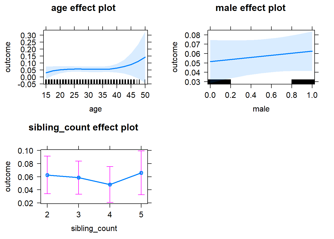
Add Birth Order Linear
Model Summary
tidy(m2_birthorder_linear, conf.int = T, conf.level = 0.995)| effect | group | term | estimate | std.error | statistic | df | p.value | conf.low | conf.high |
|---|---|---|---|---|---|---|---|---|---|
| fixed | NA | (Intercept) | -0.2049 | 0.1926 | -1.064 | 2637 | 0.2875 | -0.7457 | 0.3358 |
| fixed | NA | birth_order | 0.001188 | 0.004618 | 0.2573 | 2637 | 0.7969 | -0.01177 | 0.01415 |
| fixed | NA | poly(age, 3, raw = TRUE)1 | 0.02751 | 0.02138 | 1.287 | 2637 | 0.1984 | -0.03251 | 0.08753 |
| fixed | NA | poly(age, 3, raw = TRUE)2 | -0.0009579 | 0.0007589 | -1.262 | 2637 | 0.207 | -0.003088 | 0.001172 |
| fixed | NA | poly(age, 3, raw = TRUE)3 | 0.00001092 | 0.000008631 | 1.266 | 2637 | 0.2058 | -0.0000133 | 0.00003515 |
| fixed | NA | male | 0.01094 | 0.008989 | 1.217 | 2637 | 0.2237 | -0.01429 | 0.03617 |
| fixed | NA | sibling_count3 | -0.004686 | 0.01227 | -0.3819 | 2637 | 0.7025 | -0.03913 | 0.02976 |
| fixed | NA | sibling_count4 | -0.0157 | 0.01345 | -1.167 | 2637 | 0.2433 | -0.05346 | 0.02206 |
| fixed | NA | sibling_count5 | 0.001332 | 0.01622 | 0.08212 | 2637 | 0.9346 | -0.0442 | 0.04687 |
| ran_pars | mother_pidlink | sd__(Intercept) | 0 | NA | NA | NA | NA | NA | NA |
| ran_pars | Residual | sd__Observation | 0.2277 | NA | NA | NA | NA | NA | NA |
Coefficient Plot
plot_birthorder2(m2_birthorder_linear, separate = FALSE)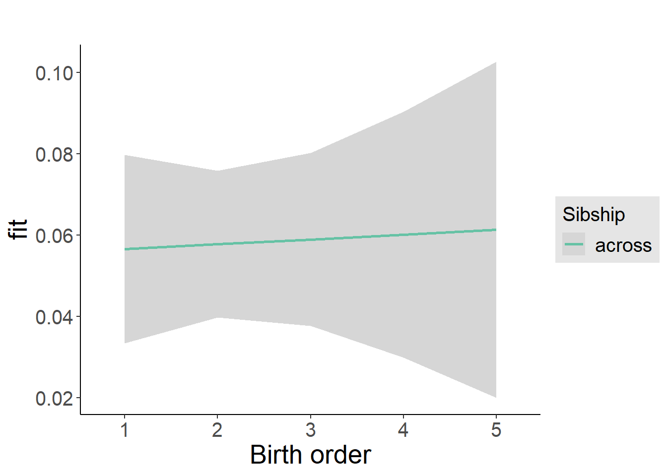
Add Birth Order Factor
Model Summary
m3_birthorder_nonlinear = update(m1_covariates_only, formula = . ~ . + birth_order_nonlinear)## boundary (singular) fit: see ?isSingulartidy(m3_birthorder_nonlinear, conf.int = T, conf.level = 0.995)| effect | group | term | estimate | std.error | statistic | df | p.value | conf.low | conf.high |
|---|---|---|---|---|---|---|---|---|---|
| fixed | NA | (Intercept) | -0.2013 | 0.1929 | -1.044 | 2634 | 0.2968 | -0.7429 | 0.3402 |
| fixed | NA | poly(age, 3, raw = TRUE)1 | 0.02774 | 0.02141 | 1.296 | 2634 | 0.1951 | -0.03235 | 0.08784 |
| fixed | NA | poly(age, 3, raw = TRUE)2 | -0.0009645 | 0.0007598 | -1.269 | 2634 | 0.2044 | -0.003097 | 0.001168 |
| fixed | NA | poly(age, 3, raw = TRUE)3 | 0.00001099 | 0.00000864 | 1.272 | 2634 | 0.2034 | -0.00001326 | 0.00003524 |
| fixed | NA | male | 0.01093 | 0.008993 | 1.215 | 2634 | 0.2244 | -0.01431 | 0.03617 |
| fixed | NA | sibling_count3 | -0.006049 | 0.01248 | -0.4848 | 2634 | 0.6278 | -0.04107 | 0.02897 |
| fixed | NA | sibling_count4 | -0.01936 | 0.01365 | -1.419 | 2634 | 0.1562 | -0.05766 | 0.01895 |
| fixed | NA | sibling_count5 | -0.0001196 | 0.0165 | -0.007248 | 2634 | 0.9942 | -0.04644 | 0.0462 |
| fixed | NA | birth_order_nonlinear2 | -0.01424 | 0.01083 | -1.315 | 2634 | 0.1887 | -0.04463 | 0.01616 |
| fixed | NA | birth_order_nonlinear3 | 0.006096 | 0.01329 | 0.4587 | 2634 | 0.6465 | -0.03121 | 0.0434 |
| fixed | NA | birth_order_nonlinear4 | 0.01221 | 0.01818 | 0.6715 | 2634 | 0.502 | -0.03883 | 0.06325 |
| fixed | NA | birth_order_nonlinear5 | -0.01491 | 0.02909 | -0.5124 | 2634 | 0.6084 | -0.09657 | 0.06676 |
| ran_pars | mother_pidlink | sd__(Intercept) | 0 | NA | NA | NA | NA | NA | NA |
| ran_pars | Residual | sd__Observation | 0.2276 | NA | NA | NA | NA | NA | NA |
Coefficient Plot
plot_birthorder(m3_birthorder_nonlinear, separate = FALSE)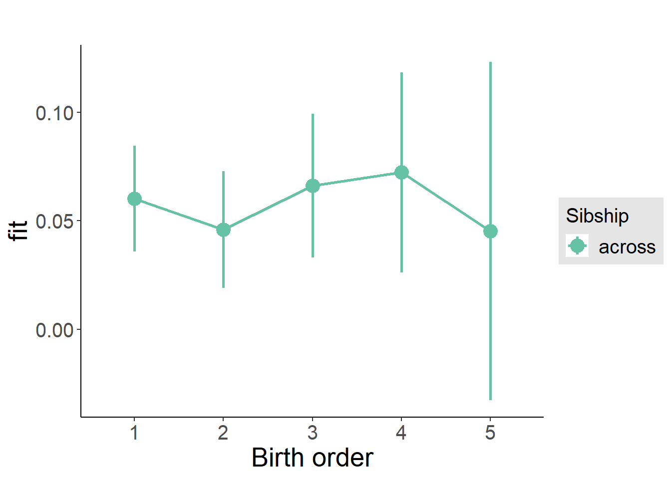
Add Interaction
Model Summary
m4_interaction = update(m3_birthorder_nonlinear, formula = . ~ . - birth_order_nonlinear - sibling_count + count_birth_order)## boundary (singular) fit: see ?isSingulartidy(m4_interaction, conf.int = T, conf.level = 0.995)| effect | group | term | estimate | std.error | statistic | df | p.value | conf.low | conf.high |
|---|---|---|---|---|---|---|---|---|---|
| fixed | NA | (Intercept) | -0.2 | 0.1932 | -1.035 | 2628 | 0.3006 | -0.7422 | 0.3422 |
| fixed | NA | poly(age, 3, raw = TRUE)1 | 0.02738 | 0.02144 | 1.277 | 2628 | 0.2016 | -0.03279 | 0.08755 |
| fixed | NA | poly(age, 3, raw = TRUE)2 | -0.0009506 | 0.0007609 | -1.249 | 2628 | 0.2117 | -0.003087 | 0.001185 |
| fixed | NA | poly(age, 3, raw = TRUE)3 | 0.00001081 | 0.000008654 | 1.25 | 2628 | 0.2116 | -0.00001348 | 0.00003511 |
| fixed | NA | male | 0.01061 | 0.009007 | 1.178 | 2628 | 0.2391 | -0.01468 | 0.03589 |
| fixed | NA | count_birth_order2/2 | -0.008312 | 0.01941 | -0.4281 | 2628 | 0.6686 | -0.0628 | 0.04618 |
| fixed | NA | count_birth_order1/3 | -0.005054 | 0.01622 | -0.3116 | 2628 | 0.7554 | -0.05058 | 0.04047 |
| fixed | NA | count_birth_order2/3 | -0.02742 | 0.01804 | -1.52 | 2628 | 0.1287 | -0.07806 | 0.02323 |
| fixed | NA | count_birth_order3/3 | 0.01547 | 0.01945 | 0.7955 | 2628 | 0.4264 | -0.03912 | 0.07007 |
| fixed | NA | count_birth_order1/4 | -0.01451 | 0.01908 | -0.7606 | 2628 | 0.447 | -0.06809 | 0.03906 |
| fixed | NA | count_birth_order2/4 | -0.02173 | 0.02003 | -1.085 | 2628 | 0.2782 | -0.07796 | 0.0345 |
| fixed | NA | count_birth_order3/4 | -0.0271 | 0.0208 | -1.303 | 2628 | 0.1926 | -0.08548 | 0.03127 |
| fixed | NA | count_birth_order4/4 | -0.003558 | 0.02257 | -0.1577 | 2628 | 0.8747 | -0.0669 | 0.05979 |
| fixed | NA | count_birth_order1/5 | 0.007468 | 0.02502 | 0.2984 | 2628 | 0.7654 | -0.06277 | 0.0777 |
| fixed | NA | count_birth_order2/5 | -0.01613 | 0.02789 | -0.5784 | 2628 | 0.563 | -0.09442 | 0.06216 |
| fixed | NA | count_birth_order3/5 | 0.007383 | 0.02716 | 0.2718 | 2628 | 0.7858 | -0.06886 | 0.08363 |
| fixed | NA | count_birth_order4/5 | 0.01181 | 0.02613 | 0.4519 | 2628 | 0.6514 | -0.06154 | 0.08515 |
| fixed | NA | count_birth_order5/5 | -0.01303 | 0.02775 | -0.4695 | 2628 | 0.6388 | -0.09093 | 0.06487 |
| ran_pars | mother_pidlink | sd__(Intercept) | 0.000000003253 | NA | NA | NA | NA | NA | NA |
| ran_pars | Residual | sd__Observation | 0.2278 | NA | NA | NA | NA | NA | NA |
Coefficient Plot
plot_birthorder(m4_interaction)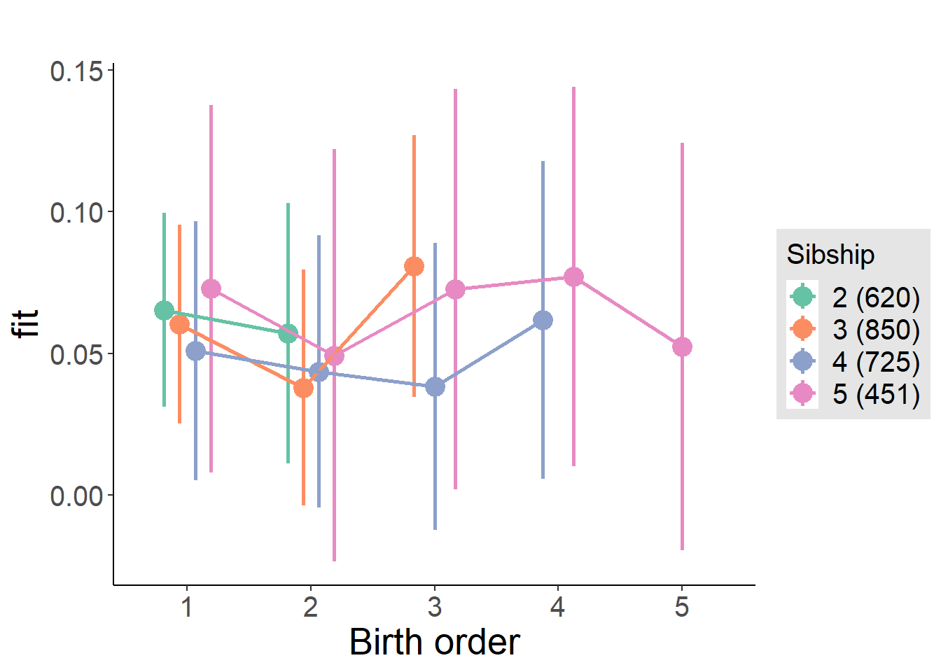
Model Comparison
###### Model 1 - Model 2
anova(m1_covariates_only, m2_birthorder_linear, m3_birthorder_nonlinear, m4_interaction)## refitting model(s) with ML (instead of REML)| Df | AIC | BIC | logLik | deviance | Chisq | Chi Df | Pr(>Chisq) |
|---|---|---|---|---|---|---|---|
| 10 | -311.1 | -252.3 | 165.6 | -331.1 | NA | NA | NA |
| 11 | -309.2 | -244.5 | 165.6 | -331.2 | 0.06645 | 1 | 0.7966 |
| 14 | -307 | -224.6 | 167.5 | -335 | 3.759 | 3 | 0.2887 |
| 20 | -297.5 | -179.9 | 168.8 | -337.5 | 2.584 | 6 | 0.859 |
Compare birth order specifications
library(coefplot)
multiplot(outcome_naive_m1, outcome_preg_m1, outcome_uterus_m1, outcome_parental_m1, dodgeHeight = 0.6,
intercept = FALSE)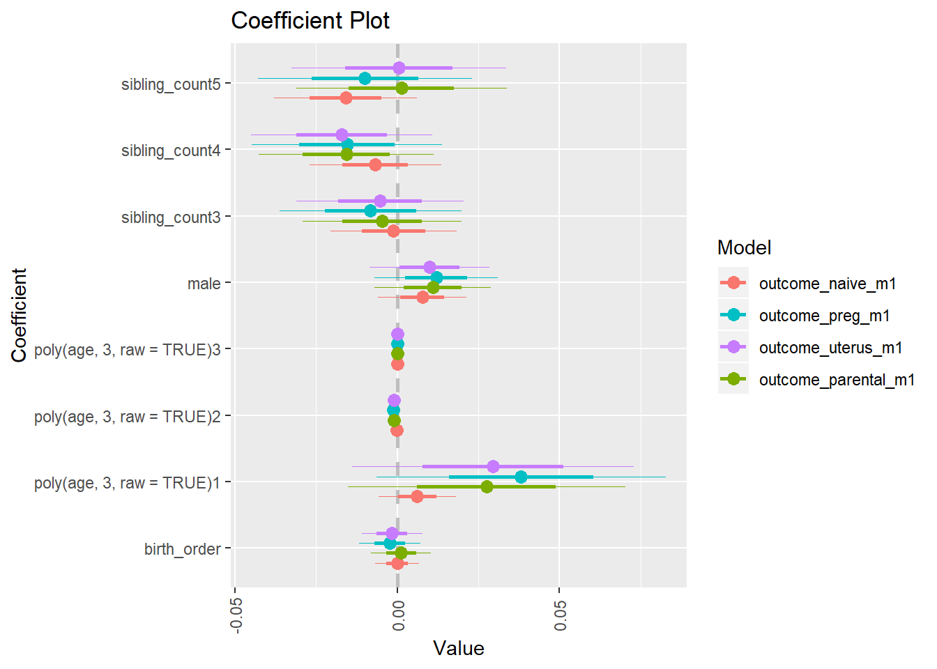
Sector_Transportation, storage and communications
birthorder <- birthorder %>% mutate(outcome = `Sector_Transportation, storage and communications`)
model = lmer(outcome ~ birth_order + poly(age, 3, raw = TRUE) + male + sibling_count + (1 | mother_pidlink),
data = birthorder)
compare_birthorder_specs(model)Naive birth order
outcome_naive_m1 <- update(m2_birthorder_linear, data = birthorder %>%
mutate(sibling_count = sibling_count_naive_factor,
birth_order_nonlinear = birthorder_naive_factor,
birth_order = birthorder_naive,
count_birth_order = count_birthorder_naive) %>%
filter(sibling_count != "1"))
compare_models_markdown(outcome_naive_m1)Basic Model
Model Summary
m1_covariates_only <- update(m2_birthorder_linear, formula = . ~ . - birth_order)
tidy(m1_covariates_only, conf.int = T, conf.level = 0.995)| effect | group | term | estimate | std.error | statistic | df | p.value | conf.low | conf.high |
|---|---|---|---|---|---|---|---|---|---|
| fixed | NA | (Intercept) | 0.1106 | 0.05168 | 2.14 | 4215 | 0.0324 | -0.03447 | 0.2557 |
| fixed | NA | poly(age, 3, raw = TRUE)1 | -0.007407 | 0.004589 | -1.614 | 4077 | 0.1066 | -0.02029 | 0.005474 |
| fixed | NA | poly(age, 3, raw = TRUE)2 | 0.0001961 | 0.0001268 | 1.546 | 3932 | 0.1221 | -0.0001599 | 0.0005521 |
| fixed | NA | poly(age, 3, raw = TRUE)3 | -0.000001494 | 0.000001104 | -1.353 | 3812 | 0.176 | -0.000004594 | 0.000001605 |
| fixed | NA | male | -0.01298 | 0.005339 | -2.431 | 4632 | 0.0151 | -0.02797 | 0.002009 |
| fixed | NA | sibling_count3 | 0.009016 | 0.007479 | 1.205 | 3447 | 0.2281 | -0.01198 | 0.03001 |
| fixed | NA | sibling_count4 | 0.01098 | 0.007539 | 1.457 | 3133 | 0.1453 | -0.01018 | 0.03214 |
| fixed | NA | sibling_count5 | 0.0234 | 0.007815 | 2.995 | 2849 | 0.002771 | 0.001466 | 0.04534 |
| ran_pars | mother_pidlink | sd__(Intercept) | 0.02411 | NA | NA | NA | NA | NA | NA |
| ran_pars | Residual | sd__Observation | 0.1784 | NA | NA | NA | NA | NA | NA |
Coefficient Plot
plot(allEffects(m1_covariates_only, confidence.level = 0.995))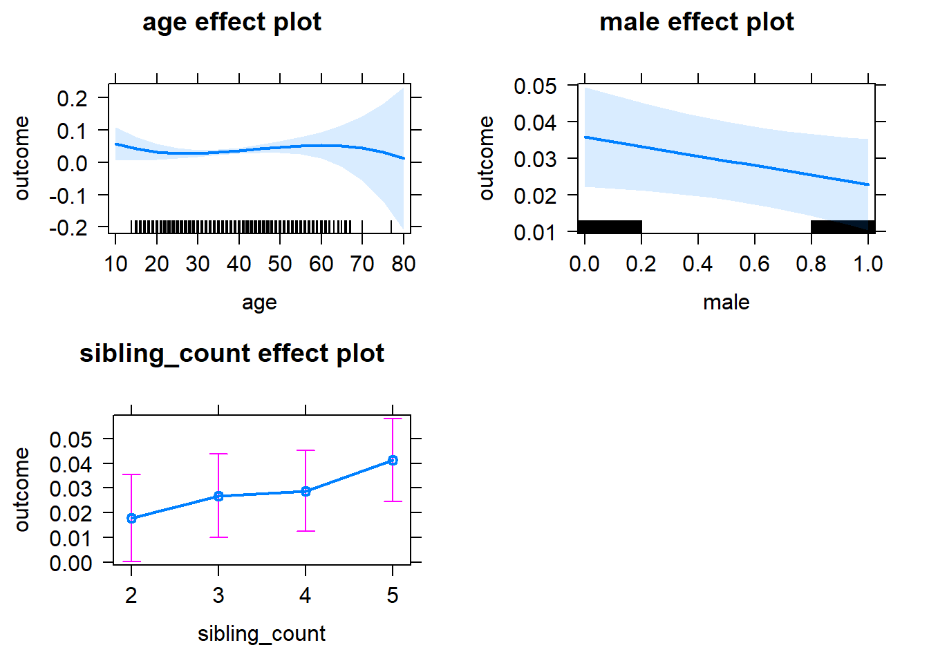
Add Birth Order Linear
Model Summary
tidy(m2_birthorder_linear, conf.int = T, conf.level = 0.995)| effect | group | term | estimate | std.error | statistic | df | p.value | conf.low | conf.high |
|---|---|---|---|---|---|---|---|---|---|
| fixed | NA | (Intercept) | 0.1111 | 0.05168 | 2.149 | 4214 | 0.03168 | -0.034 | 0.2561 |
| fixed | NA | birth_order | 0.00181 | 0.002653 | 0.6821 | 4285 | 0.4952 | -0.005638 | 0.009258 |
| fixed | NA | poly(age, 3, raw = TRUE)1 | -0.00768 | 0.004606 | -1.667 | 4076 | 0.09555 | -0.02061 | 0.00525 |
| fixed | NA | poly(age, 3, raw = TRUE)2 | 0.0002029 | 0.0001272 | 1.595 | 3924 | 0.1109 | -0.0001542 | 0.0005599 |
| fixed | NA | poly(age, 3, raw = TRUE)3 | -0.00000154 | 0.000001106 | -1.392 | 3804 | 0.1639 | -0.000004645 | 0.000001565 |
| fixed | NA | male | -0.01296 | 0.00534 | -2.427 | 4631 | 0.01527 | -0.02795 | 0.00203 |
| fixed | NA | sibling_count3 | 0.008324 | 0.007548 | 1.103 | 3532 | 0.2702 | -0.01286 | 0.02951 |
| fixed | NA | sibling_count4 | 0.009485 | 0.00785 | 1.208 | 3496 | 0.227 | -0.01255 | 0.03152 |
| fixed | NA | sibling_count5 | 0.02105 | 0.008542 | 2.464 | 3581 | 0.01379 | -0.00293 | 0.04502 |
| ran_pars | mother_pidlink | sd__(Intercept) | 0.02369 | NA | NA | NA | NA | NA | NA |
| ran_pars | Residual | sd__Observation | 0.1784 | NA | NA | NA | NA | NA | NA |
Coefficient Plot
plot_birthorder2(m2_birthorder_linear, separate = FALSE)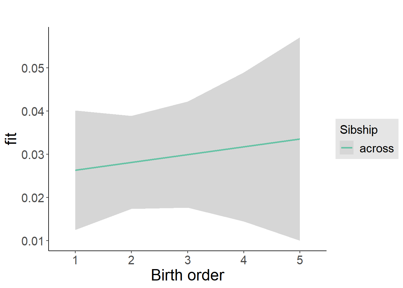
Add Birth Order Factor
Model Summary
m3_birthorder_nonlinear = update(m1_covariates_only, formula = . ~ . + birth_order_nonlinear)
tidy(m3_birthorder_nonlinear, conf.int = T, conf.level = 0.995)| effect | group | term | estimate | std.error | statistic | df | p.value | conf.low | conf.high |
|---|---|---|---|---|---|---|---|---|---|
| fixed | NA | (Intercept) | 0.1115 | 0.05184 | 2.151 | 4219 | 0.03153 | -0.03401 | 0.257 |
| fixed | NA | poly(age, 3, raw = TRUE)1 | -0.00755 | 0.004606 | -1.639 | 4072 | 0.1013 | -0.02048 | 0.005381 |
| fixed | NA | poly(age, 3, raw = TRUE)2 | 0.0001993 | 0.0001272 | 1.567 | 3916 | 0.1173 | -0.0001578 | 0.0005565 |
| fixed | NA | poly(age, 3, raw = TRUE)3 | -0.00000151 | 0.000001107 | -1.364 | 3789 | 0.1725 | -0.000004617 | 0.000001597 |
| fixed | NA | male | -0.01274 | 0.005341 | -2.386 | 4628 | 0.01705 | -0.02774 | 0.002246 |
| fixed | NA | sibling_count3 | 0.006757 | 0.007691 | 0.8786 | 3684 | 0.3797 | -0.01483 | 0.02834 |
| fixed | NA | sibling_count4 | 0.01084 | 0.008007 | 1.354 | 3666 | 0.1758 | -0.01163 | 0.03332 |
| fixed | NA | sibling_count5 | 0.01992 | 0.008636 | 2.307 | 3678 | 0.02112 | -0.004319 | 0.04416 |
| fixed | NA | birth_order_nonlinear2 | 0.001177 | 0.006405 | 0.1838 | 4156 | 0.8542 | -0.0168 | 0.01916 |
| fixed | NA | birth_order_nonlinear3 | 0.009914 | 0.008122 | 1.221 | 4158 | 0.2223 | -0.01288 | 0.03271 |
| fixed | NA | birth_order_nonlinear4 | -0.00988 | 0.01061 | -0.931 | 4160 | 0.3519 | -0.03967 | 0.01991 |
| fixed | NA | birth_order_nonlinear5 | 0.02139 | 0.0153 | 1.398 | 4235 | 0.1623 | -0.02157 | 0.06435 |
| ran_pars | mother_pidlink | sd__(Intercept) | 0.02371 | NA | NA | NA | NA | NA | NA |
| ran_pars | Residual | sd__Observation | 0.1784 | NA | NA | NA | NA | NA | NA |
Coefficient Plot
plot_birthorder(m3_birthorder_nonlinear, separate = FALSE)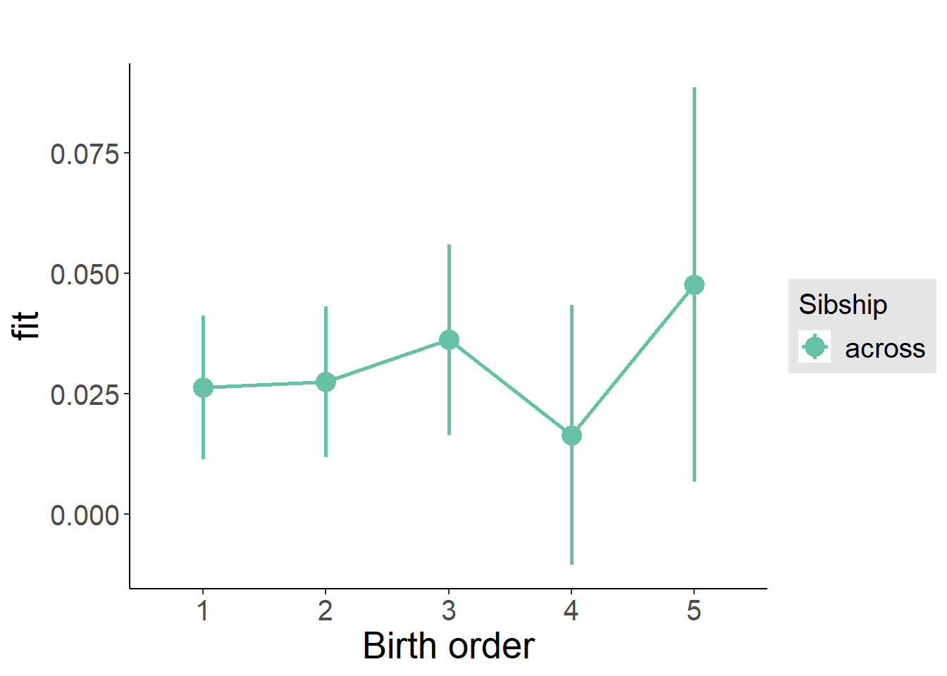
Add Interaction
Model Summary
m4_interaction = update(m3_birthorder_nonlinear, formula = . ~ . - birth_order_nonlinear - sibling_count + count_birth_order)
tidy(m4_interaction, conf.int = T, conf.level = 0.995)| effect | group | term | estimate | std.error | statistic | df | p.value | conf.low | conf.high |
|---|---|---|---|---|---|---|---|---|---|
| fixed | NA | (Intercept) | 0.1132 | 0.05194 | 2.179 | 4223 | 0.0294 | -0.03263 | 0.259 |
| fixed | NA | poly(age, 3, raw = TRUE)1 | -0.00751 | 0.004612 | -1.628 | 4068 | 0.1035 | -0.02046 | 0.005436 |
| fixed | NA | poly(age, 3, raw = TRUE)2 | 0.0001992 | 0.0001273 | 1.564 | 3912 | 0.1178 | -0.0001582 | 0.0005566 |
| fixed | NA | poly(age, 3, raw = TRUE)3 | -0.000001516 | 0.000001107 | -1.369 | 3785 | 0.1711 | -0.000004624 | 0.000001592 |
| fixed | NA | male | -0.01268 | 0.005344 | -2.374 | 4621 | 0.01766 | -0.02769 | 0.002317 |
| fixed | NA | count_birth_order2/2 | -0.005555 | 0.01092 | -0.5089 | 4038 | 0.6109 | -0.0362 | 0.02509 |
| fixed | NA | count_birth_order1/3 | 0.003489 | 0.01032 | 0.338 | 4624 | 0.7354 | -0.02548 | 0.03246 |
| fixed | NA | count_birth_order2/3 | 0.00642 | 0.01149 | 0.5586 | 4624 | 0.5764 | -0.02584 | 0.03868 |
| fixed | NA | count_birth_order3/3 | 0.01413 | 0.01264 | 1.118 | 4624 | 0.2638 | -0.02136 | 0.04963 |
| fixed | NA | count_birth_order1/4 | 0.01342 | 0.01137 | 1.18 | 4625 | 0.2382 | -0.01851 | 0.04535 |
| fixed | NA | count_birth_order2/4 | 0.007184 | 0.0122 | 0.5887 | 4624 | 0.5561 | -0.02707 | 0.04144 |
| fixed | NA | count_birth_order3/4 | 0.01613 | 0.01288 | 1.252 | 4624 | 0.2106 | -0.02003 | 0.05228 |
| fixed | NA | count_birth_order4/4 | -0.004703 | 0.01389 | -0.3386 | 4623 | 0.7349 | -0.04369 | 0.03428 |
| fixed | NA | count_birth_order1/5 | 0.004813 | 0.01283 | 0.375 | 4625 | 0.7077 | -0.03121 | 0.04084 |
| fixed | NA | count_birth_order2/5 | 0.02775 | 0.01364 | 2.034 | 4625 | 0.04198 | -0.01054 | 0.06604 |
| fixed | NA | count_birth_order3/5 | 0.03003 | 0.01435 | 2.092 | 4625 | 0.03649 | -0.01026 | 0.07031 |
| fixed | NA | count_birth_order4/5 | 0.01143 | 0.01517 | 0.7536 | 4625 | 0.4511 | -0.03115 | 0.05401 |
| fixed | NA | count_birth_order5/5 | 0.0388 | 0.0152 | 2.553 | 4624 | 0.01072 | -0.003867 | 0.08147 |
| ran_pars | mother_pidlink | sd__(Intercept) | 0.02323 | NA | NA | NA | NA | NA | NA |
| ran_pars | Residual | sd__Observation | 0.1785 | NA | NA | NA | NA | NA | NA |
Coefficient Plot
plot_birthorder(m4_interaction)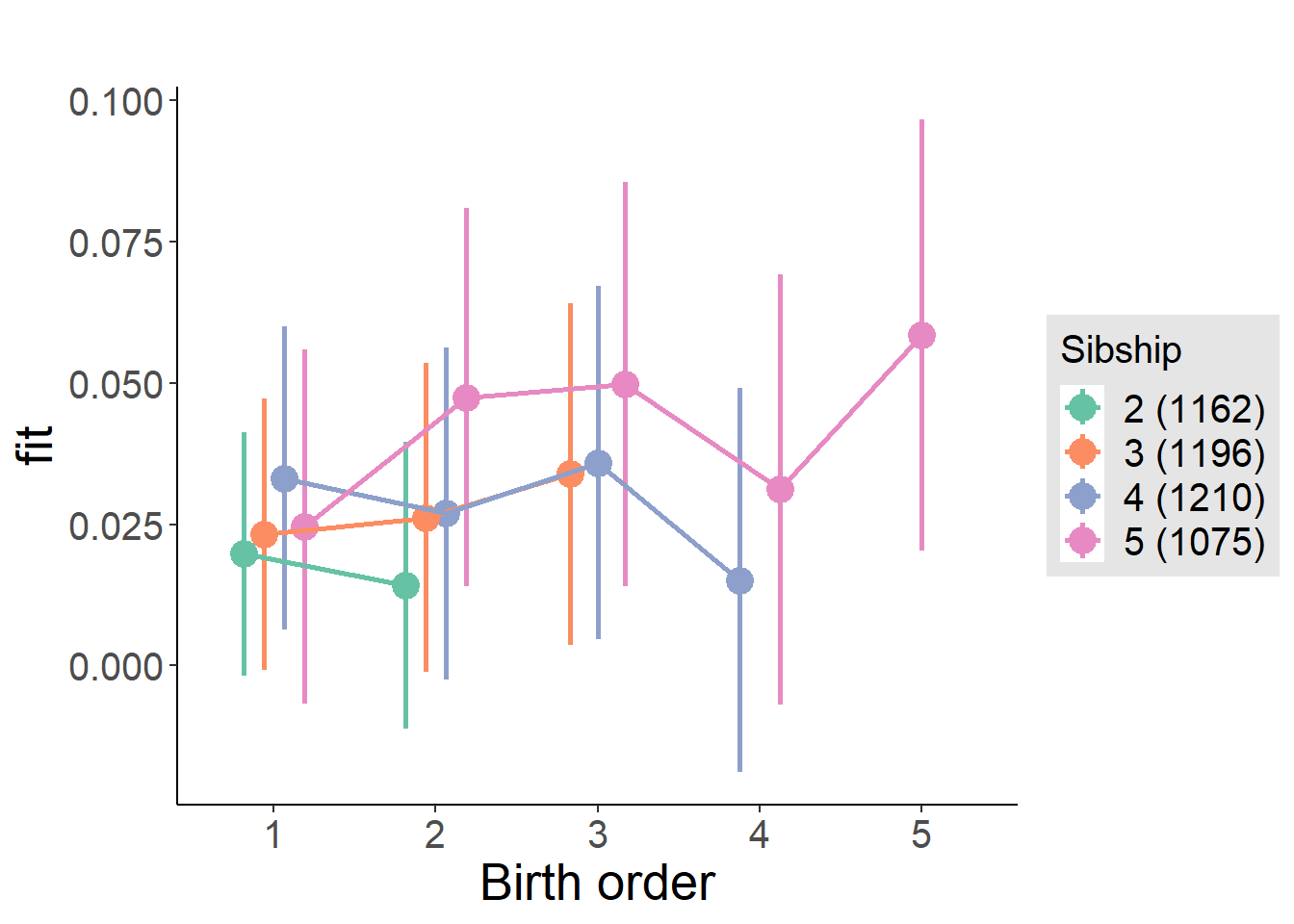
Model Comparison
###### Model 1 - Model 2
anova(m1_covariates_only, m2_birthorder_linear, m3_birthorder_nonlinear, m4_interaction)## refitting model(s) with ML (instead of REML)| Df | AIC | BIC | logLik | deviance | Chisq | Chi Df | Pr(>Chisq) |
|---|---|---|---|---|---|---|---|
| 10 | -2736 | -2672 | 1378 | -2756 | NA | NA | NA |
| 11 | -2735 | -2664 | 1378 | -2757 | 0.4679 | 1 | 0.494 |
| 14 | -2734 | -2643 | 1381 | -2762 | 4.864 | 3 | 0.182 |
| 20 | -2725 | -2596 | 1382 | -2765 | 2.98 | 6 | 0.8114 |
Maternal birth order
outcome_uterus_m1 <- update(m2_birthorder_linear, data = birthorder %>%
mutate(sibling_count = sibling_count_uterus_alive_factor,
birth_order_nonlinear = birthorder_uterus_alive_factor,
birth_order = birthorder_uterus_alive,
count_birth_order = count_birthorder_uterus_alive) %>%
filter(sibling_count != "1"))## boundary (singular) fit: see ?isSingularcompare_models_markdown(outcome_uterus_m1)Basic Model
Model Summary
m1_covariates_only <- update(m2_birthorder_linear, formula = . ~ . - birth_order)## boundary (singular) fit: see ?isSingulartidy(m1_covariates_only, conf.int = T, conf.level = 0.995)| effect | group | term | estimate | std.error | statistic | df | p.value | conf.low | conf.high |
|---|---|---|---|---|---|---|---|---|---|
| fixed | NA | (Intercept) | 0.185 | 0.1511 | 1.225 | 2634 | 0.2208 | -0.239 | 0.609 |
| fixed | NA | poly(age, 3, raw = TRUE)1 | -0.01421 | 0.01672 | -0.8503 | 2634 | 0.3952 | -0.06114 | 0.03271 |
| fixed | NA | poly(age, 3, raw = TRUE)2 | 0.0004341 | 0.000592 | 0.7333 | 2634 | 0.4635 | -0.001228 | 0.002096 |
| fixed | NA | poly(age, 3, raw = TRUE)3 | -0.000004419 | 0.000006715 | -0.6581 | 2634 | 0.5105 | -0.00002327 | 0.00001443 |
| fixed | NA | male | -0.01574 | 0.00712 | -2.21 | 2634 | 0.02718 | -0.03572 | 0.00425 |
| fixed | NA | sibling_count3 | 0.004938 | 0.00976 | 0.5059 | 2634 | 0.613 | -0.02246 | 0.03233 |
| fixed | NA | sibling_count4 | 0.006176 | 0.01007 | 0.6136 | 2634 | 0.5396 | -0.02208 | 0.03443 |
| fixed | NA | sibling_count5 | 0.02625 | 0.01116 | 2.352 | 2634 | 0.01874 | -0.005077 | 0.05758 |
| ran_pars | mother_pidlink | sd__(Intercept) | 0 | NA | NA | NA | NA | NA | NA |
| ran_pars | Residual | sd__Observation | 0.1802 | NA | NA | NA | NA | NA | NA |
Coefficient Plot
plot(allEffects(m1_covariates_only, confidence.level = 0.995))
Add Birth Order Linear
Model Summary
tidy(m2_birthorder_linear, conf.int = T, conf.level = 0.995)| effect | group | term | estimate | std.error | statistic | df | p.value | conf.low | conf.high |
|---|---|---|---|---|---|---|---|---|---|
| fixed | NA | (Intercept) | 0.1862 | 0.151 | 1.233 | 2633 | 0.2177 | -0.2377 | 0.6102 |
| fixed | NA | birth_order | -0.005075 | 0.00361 | -1.406 | 2633 | 0.1598 | -0.01521 | 0.005058 |
| fixed | NA | poly(age, 3, raw = TRUE)1 | -0.01377 | 0.01672 | -0.8237 | 2633 | 0.4102 | -0.06069 | 0.03315 |
| fixed | NA | poly(age, 3, raw = TRUE)2 | 0.0004271 | 0.000592 | 0.7216 | 2633 | 0.4706 | -0.001235 | 0.002089 |
| fixed | NA | poly(age, 3, raw = TRUE)3 | -0.000004466 | 0.000006714 | -0.6653 | 2633 | 0.5059 | -0.00002331 | 0.00001438 |
| fixed | NA | male | -0.01575 | 0.007119 | -2.213 | 2633 | 0.027 | -0.03574 | 0.004231 |
| fixed | NA | sibling_count3 | 0.007332 | 0.009905 | 0.7402 | 2633 | 0.4593 | -0.02047 | 0.03514 |
| fixed | NA | sibling_count4 | 0.01134 | 0.01071 | 1.059 | 2633 | 0.2898 | -0.01873 | 0.04142 |
| fixed | NA | sibling_count5 | 0.03489 | 0.01274 | 2.739 | 2633 | 0.006205 | -0.0008673 | 0.07064 |
| ran_pars | mother_pidlink | sd__(Intercept) | 0.000000002183 | NA | NA | NA | NA | NA | NA |
| ran_pars | Residual | sd__Observation | 0.1802 | NA | NA | NA | NA | NA | NA |
Coefficient Plot
plot_birthorder2(m2_birthorder_linear, separate = FALSE)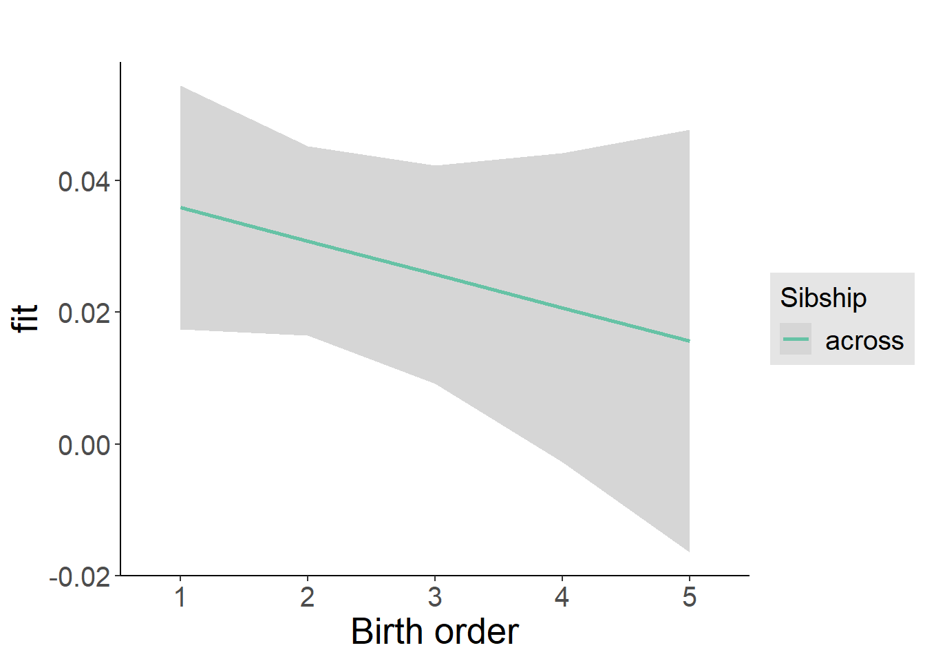
Add Birth Order Factor
Model Summary
m3_birthorder_nonlinear = update(m1_covariates_only, formula = . ~ . + birth_order_nonlinear)## boundary (singular) fit: see ?isSingulartidy(m3_birthorder_nonlinear, conf.int = T, conf.level = 0.995)| effect | group | term | estimate | std.error | statistic | df | p.value | conf.low | conf.high |
|---|---|---|---|---|---|---|---|---|---|
| fixed | NA | (Intercept) | 0.1769 | 0.1514 | 1.168 | 2630 | 0.2427 | -0.248 | 0.6018 |
| fixed | NA | poly(age, 3, raw = TRUE)1 | -0.01325 | 0.01675 | -0.7913 | 2630 | 0.4288 | -0.06027 | 0.03376 |
| fixed | NA | poly(age, 3, raw = TRUE)2 | 0.0004094 | 0.0005931 | 0.6903 | 2630 | 0.4901 | -0.001255 | 0.002074 |
| fixed | NA | poly(age, 3, raw = TRUE)3 | -0.000004277 | 0.000006726 | -0.636 | 2630 | 0.5249 | -0.00002316 | 0.0000146 |
| fixed | NA | male | -0.0157 | 0.007127 | -2.203 | 2630 | 0.0277 | -0.03571 | 0.004307 |
| fixed | NA | sibling_count3 | 0.006067 | 0.01007 | 0.6025 | 2630 | 0.5469 | -0.0222 | 0.03433 |
| fixed | NA | sibling_count4 | 0.01006 | 0.01087 | 0.9256 | 2630 | 0.3547 | -0.02046 | 0.04059 |
| fixed | NA | sibling_count5 | 0.03557 | 0.01291 | 2.755 | 2630 | 0.005917 | -0.0006773 | 0.07182 |
| fixed | NA | birth_order_nonlinear2 | -0.006373 | 0.008667 | -0.7354 | 2630 | 0.4622 | -0.0307 | 0.01795 |
| fixed | NA | birth_order_nonlinear3 | -0.004844 | 0.01055 | -0.459 | 2630 | 0.6462 | -0.03447 | 0.02478 |
| fixed | NA | birth_order_nonlinear4 | -0.0152 | 0.01403 | -1.084 | 2630 | 0.2787 | -0.05459 | 0.02418 |
| fixed | NA | birth_order_nonlinear5 | -0.03036 | 0.02176 | -1.395 | 2630 | 0.1631 | -0.09145 | 0.03073 |
| ran_pars | mother_pidlink | sd__(Intercept) | 0.000000001973 | NA | NA | NA | NA | NA | NA |
| ran_pars | Residual | sd__Observation | 0.1803 | NA | NA | NA | NA | NA | NA |
Coefficient Plot
plot_birthorder(m3_birthorder_nonlinear, separate = FALSE)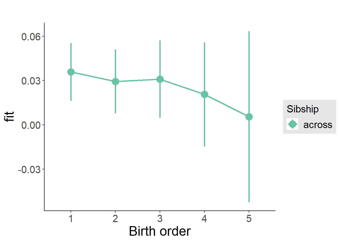
Add Interaction
Model Summary
m4_interaction = update(m3_birthorder_nonlinear, formula = . ~ . - birth_order_nonlinear - sibling_count + count_birth_order)## boundary (singular) fit: see ?isSingulartidy(m4_interaction, conf.int = T, conf.level = 0.995)| effect | group | term | estimate | std.error | statistic | df | p.value | conf.low | conf.high |
|---|---|---|---|---|---|---|---|---|---|
| fixed | NA | (Intercept) | 0.1735 | 0.1516 | 1.144 | 2624 | 0.2526 | -0.252 | 0.599 |
| fixed | NA | poly(age, 3, raw = TRUE)1 | -0.01337 | 0.01677 | -0.7972 | 2624 | 0.4254 | -0.06044 | 0.03371 |
| fixed | NA | poly(age, 3, raw = TRUE)2 | 0.0004147 | 0.0005939 | 0.6983 | 2624 | 0.485 | -0.001252 | 0.002082 |
| fixed | NA | poly(age, 3, raw = TRUE)3 | -0.000004356 | 0.000006737 | -0.6466 | 2624 | 0.5179 | -0.00002327 | 0.00001455 |
| fixed | NA | male | -0.01603 | 0.007141 | -2.245 | 2624 | 0.02487 | -0.03607 | 0.004015 |
| fixed | NA | count_birth_order2/2 | 0.007068 | 0.01581 | 0.4471 | 2624 | 0.6549 | -0.03731 | 0.05145 |
| fixed | NA | count_birth_order1/3 | 0.00987 | 0.01308 | 0.7548 | 2624 | 0.4504 | -0.02684 | 0.04658 |
| fixed | NA | count_birth_order2/3 | -0.0002422 | 0.01454 | -0.01666 | 2624 | 0.9867 | -0.04105 | 0.04056 |
| fixed | NA | count_birth_order3/3 | 0.01252 | 0.01585 | 0.7898 | 2624 | 0.4297 | -0.03197 | 0.057 |
| fixed | NA | count_birth_order1/4 | 0.02086 | 0.01504 | 1.387 | 2624 | 0.1656 | -0.02136 | 0.06309 |
| fixed | NA | count_birth_order2/4 | 0.009328 | 0.01593 | 0.5855 | 2624 | 0.5582 | -0.03539 | 0.05405 |
| fixed | NA | count_birth_order3/4 | 0.0003236 | 0.01653 | 0.01958 | 2624 | 0.9844 | -0.04607 | 0.04672 |
| fixed | NA | count_birth_order4/4 | -0.001404 | 0.01767 | -0.07945 | 2624 | 0.9367 | -0.05101 | 0.0482 |
| fixed | NA | count_birth_order1/5 | 0.0448 | 0.01987 | 2.255 | 2624 | 0.0242 | -0.01096 | 0.1006 |
| fixed | NA | count_birth_order2/5 | 0.02365 | 0.02139 | 1.106 | 2624 | 0.2689 | -0.03638 | 0.08368 |
| fixed | NA | count_birth_order3/5 | 0.03798 | 0.02031 | 1.87 | 2624 | 0.06163 | -0.01904 | 0.095 |
| fixed | NA | count_birth_order4/5 | 0.02571 | 0.0198 | 1.298 | 2624 | 0.1944 | -0.02988 | 0.08129 |
| fixed | NA | count_birth_order5/5 | 0.009607 | 0.02084 | 0.4611 | 2624 | 0.6448 | -0.04888 | 0.0681 |
| ran_pars | mother_pidlink | sd__(Intercept) | 0 | NA | NA | NA | NA | NA | NA |
| ran_pars | Residual | sd__Observation | 0.1804 | NA | NA | NA | NA | NA | NA |
Coefficient Plot
plot_birthorder(m4_interaction)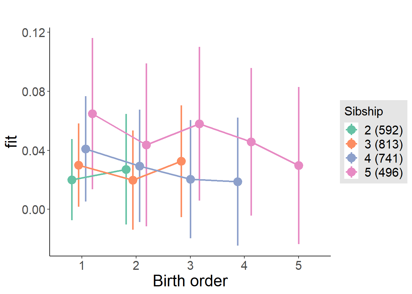
Model Comparison
###### Model 1 - Model 2
anova(m1_covariates_only, m2_birthorder_linear, m3_birthorder_nonlinear, m4_interaction)## refitting model(s) with ML (instead of REML)| Df | AIC | BIC | logLik | deviance | Chisq | Chi Df | Pr(>Chisq) |
|---|---|---|---|---|---|---|---|
| 10 | -1545 | -1486 | 782.3 | -1565 | NA | NA | NA |
| 11 | -1545 | -1480 | 783.3 | -1567 | 1.983 | 1 | 0.1591 |
| 14 | -1539 | -1457 | 783.7 | -1567 | 0.6754 | 3 | 0.879 |
| 20 | -1530 | -1412 | 784.8 | -1570 | 2.307 | 6 | 0.8894 |
Maternal pregnancy order
outcome_preg_m1 <- update(m2_birthorder_linear, data = birthorder %>%
mutate(sibling_count = sibling_count_uterus_preg_factor,
birth_order_nonlinear = birthorder_uterus_preg_factor,
birth_order = birthorder_uterus_preg,
count_birth_order = count_birthorder_uterus_preg
) %>%
filter(sibling_count != "1"))## boundary (singular) fit: see ?isSingularcompare_models_markdown(outcome_preg_m1)Basic Model
Model Summary
m1_covariates_only <- update(m2_birthorder_linear, formula = . ~ . - birth_order)## boundary (singular) fit: see ?isSingulartidy(m1_covariates_only, conf.int = T, conf.level = 0.995)| effect | group | term | estimate | std.error | statistic | df | p.value | conf.low | conf.high |
|---|---|---|---|---|---|---|---|---|---|
| fixed | NA | (Intercept) | 0.1902 | 0.1546 | 1.23 | 2419 | 0.2188 | -0.2438 | 0.6242 |
| fixed | NA | poly(age, 3, raw = TRUE)1 | -0.01507 | 0.01712 | -0.8803 | 2419 | 0.3788 | -0.06313 | 0.03299 |
| fixed | NA | poly(age, 3, raw = TRUE)2 | 0.0004658 | 0.0006064 | 0.7681 | 2419 | 0.4425 | -0.001236 | 0.002168 |
| fixed | NA | poly(age, 3, raw = TRUE)3 | -0.000004832 | 0.000006879 | -0.7025 | 2419 | 0.4825 | -0.00002414 | 0.00001448 |
| fixed | NA | male | -0.01975 | 0.007343 | -2.69 | 2419 | 0.007186 | -0.04036 | 0.0008565 |
| fixed | NA | sibling_count3 | 0.01015 | 0.01059 | 0.9585 | 2419 | 0.3379 | -0.01957 | 0.03986 |
| fixed | NA | sibling_count4 | 0.00702 | 0.01069 | 0.6568 | 2419 | 0.5113 | -0.02298 | 0.03702 |
| fixed | NA | sibling_count5 | 0.03426 | 0.01123 | 3.05 | 2419 | 0.002313 | 0.002728 | 0.06578 |
| ran_pars | mother_pidlink | sd__(Intercept) | 0.000000002039 | NA | NA | NA | NA | NA | NA |
| ran_pars | Residual | sd__Observation | 0.1781 | NA | NA | NA | NA | NA | NA |
Coefficient Plot
plot(allEffects(m1_covariates_only, confidence.level = 0.995))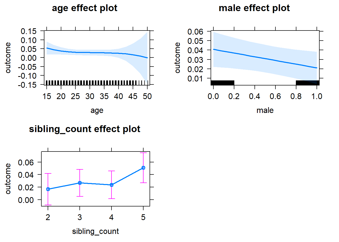
Add Birth Order Linear
Model Summary
tidy(m2_birthorder_linear, conf.int = T, conf.level = 0.995)| effect | group | term | estimate | std.error | statistic | df | p.value | conf.low | conf.high |
|---|---|---|---|---|---|---|---|---|---|
| fixed | NA | (Intercept) | 0.1911 | 0.1547 | 1.235 | 2418 | 0.2168 | -0.2431 | 0.6252 |
| fixed | NA | birth_order | -0.00116 | 0.003613 | -0.3211 | 2418 | 0.7482 | -0.0113 | 0.008983 |
| fixed | NA | poly(age, 3, raw = TRUE)1 | -0.01502 | 0.01713 | -0.8773 | 2418 | 0.3804 | -0.0631 | 0.03305 |
| fixed | NA | poly(age, 3, raw = TRUE)2 | 0.0004657 | 0.0006065 | 0.7677 | 2418 | 0.4427 | -0.001237 | 0.002168 |
| fixed | NA | poly(age, 3, raw = TRUE)3 | -0.000004856 | 0.000006881 | -0.7058 | 2418 | 0.4804 | -0.00002417 | 0.00001446 |
| fixed | NA | male | -0.01979 | 0.007345 | -2.694 | 2418 | 0.007103 | -0.04041 | 0.000828 |
| fixed | NA | sibling_count3 | 0.0107 | 0.01073 | 0.9973 | 2418 | 0.3187 | -0.01941 | 0.0408 |
| fixed | NA | sibling_count4 | 0.00811 | 0.01122 | 0.7231 | 2418 | 0.4697 | -0.02337 | 0.03959 |
| fixed | NA | sibling_count5 | 0.0361 | 0.01262 | 2.86 | 2418 | 0.004269 | 0.0006722 | 0.07153 |
| ran_pars | mother_pidlink | sd__(Intercept) | 0 | NA | NA | NA | NA | NA | NA |
| ran_pars | Residual | sd__Observation | 0.1781 | NA | NA | NA | NA | NA | NA |
Coefficient Plot
plot_birthorder2(m2_birthorder_linear, separate = FALSE)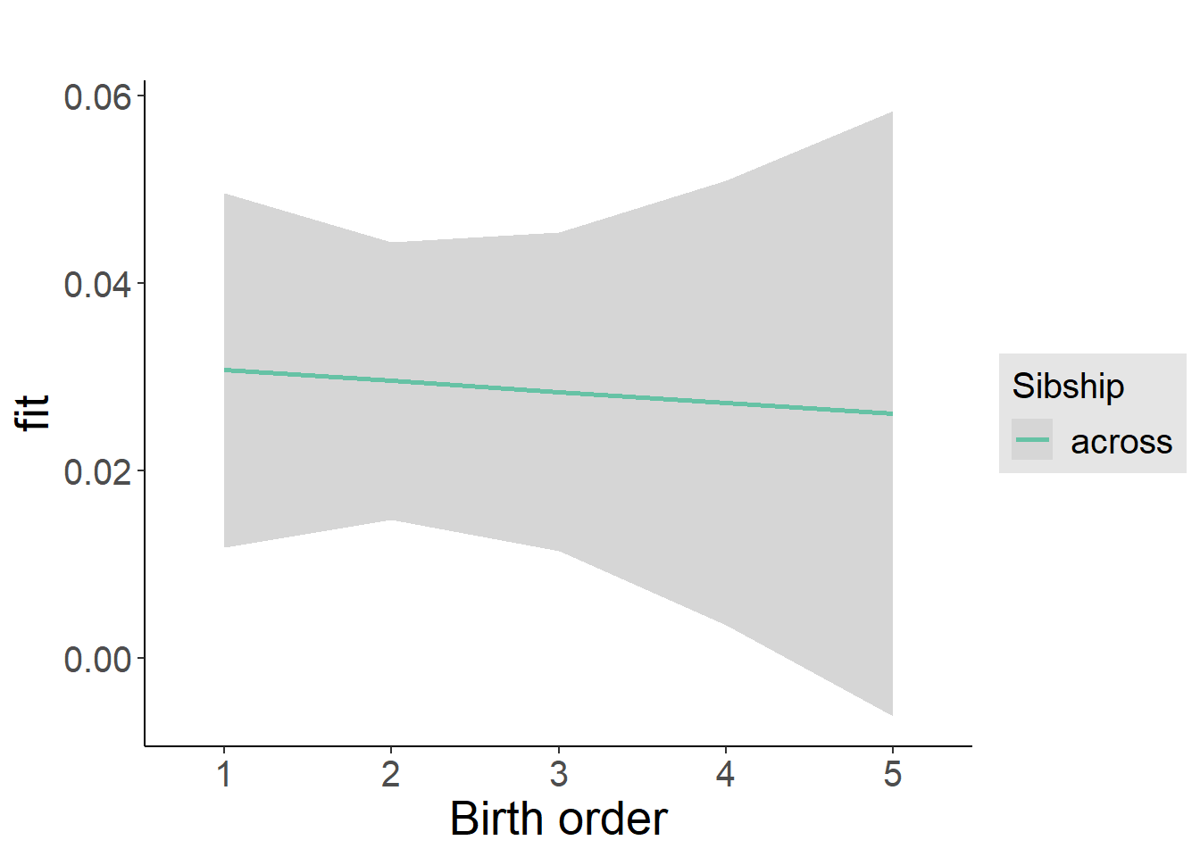
Add Birth Order Factor
Model Summary
m3_birthorder_nonlinear = update(m1_covariates_only, formula = . ~ . + birth_order_nonlinear)## boundary (singular) fit: see ?isSingulartidy(m3_birthorder_nonlinear, conf.int = T, conf.level = 0.995)| effect | group | term | estimate | std.error | statistic | df | p.value | conf.low | conf.high |
|---|---|---|---|---|---|---|---|---|---|
| fixed | NA | (Intercept) | 0.1911 | 0.1551 | 1.232 | 2415 | 0.218 | -0.2443 | 0.6265 |
| fixed | NA | poly(age, 3, raw = TRUE)1 | -0.01505 | 0.01717 | -0.8763 | 2415 | 0.381 | -0.06325 | 0.03315 |
| fixed | NA | poly(age, 3, raw = TRUE)2 | 0.0004673 | 0.0006081 | 0.7684 | 2415 | 0.4423 | -0.00124 | 0.002174 |
| fixed | NA | poly(age, 3, raw = TRUE)3 | -0.00000488 | 0.000006898 | -0.7075 | 2415 | 0.4793 | -0.00002424 | 0.00001448 |
| fixed | NA | male | -0.01987 | 0.007354 | -2.702 | 2415 | 0.006933 | -0.04052 | 0.0007697 |
| fixed | NA | sibling_count3 | 0.01065 | 0.01089 | 0.9777 | 2415 | 0.3283 | -0.01993 | 0.04122 |
| fixed | NA | sibling_count4 | 0.007511 | 0.01137 | 0.6606 | 2415 | 0.509 | -0.02441 | 0.03943 |
| fixed | NA | sibling_count5 | 0.03579 | 0.01271 | 2.815 | 2415 | 0.004921 | 0.00009795 | 0.07147 |
| fixed | NA | birth_order_nonlinear2 | -0.004707 | 0.008881 | -0.53 | 2415 | 0.5961 | -0.02964 | 0.02022 |
| fixed | NA | birth_order_nonlinear3 | -0.00238 | 0.01092 | -0.218 | 2415 | 0.8275 | -0.03303 | 0.02827 |
| fixed | NA | birth_order_nonlinear4 | -0.001274 | 0.01438 | -0.08861 | 2415 | 0.9294 | -0.04165 | 0.0391 |
| fixed | NA | birth_order_nonlinear5 | -0.007768 | 0.02068 | -0.3755 | 2415 | 0.7073 | -0.06583 | 0.05029 |
| ran_pars | mother_pidlink | sd__(Intercept) | 0 | NA | NA | NA | NA | NA | NA |
| ran_pars | Residual | sd__Observation | 0.1782 | NA | NA | NA | NA | NA | NA |
Coefficient Plot
plot_birthorder(m3_birthorder_nonlinear, separate = FALSE)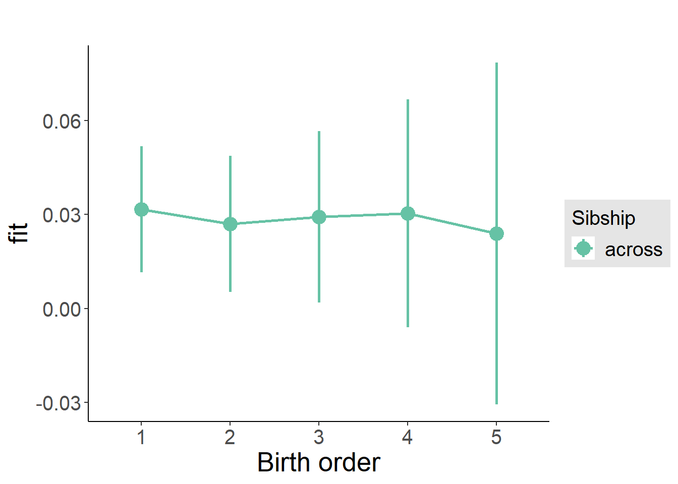
Add Interaction
Model Summary
m4_interaction = update(m3_birthorder_nonlinear, formula = . ~ . - birth_order_nonlinear - sibling_count + count_birth_order)## boundary (singular) fit: see ?isSingulartidy(m4_interaction, conf.int = T, conf.level = 0.995)| effect | group | term | estimate | std.error | statistic | df | p.value | conf.low | conf.high |
|---|---|---|---|---|---|---|---|---|---|
| fixed | NA | (Intercept) | 0.1648 | 0.1549 | 1.064 | 2409 | 0.2875 | -0.27 | 0.5997 |
| fixed | NA | poly(age, 3, raw = TRUE)1 | -0.01283 | 0.01715 | -0.7481 | 2409 | 0.4545 | -0.06098 | 0.03531 |
| fixed | NA | poly(age, 3, raw = TRUE)2 | 0.0003896 | 0.0006074 | 0.6414 | 2409 | 0.5213 | -0.001315 | 0.002095 |
| fixed | NA | poly(age, 3, raw = TRUE)3 | -0.000004026 | 0.00000689 | -0.5843 | 2409 | 0.5591 | -0.00002337 | 0.00001532 |
| fixed | NA | male | -0.01961 | 0.007352 | -2.668 | 2409 | 0.007684 | -0.04025 | 0.001023 |
| fixed | NA | count_birth_order2/2 | 0.01414 | 0.01707 | 0.8283 | 2409 | 0.4076 | -0.03377 | 0.06204 |
| fixed | NA | count_birth_order1/3 | 0.015 | 0.01426 | 1.052 | 2409 | 0.2929 | -0.02503 | 0.05503 |
| fixed | NA | count_birth_order2/3 | 0.005775 | 0.01552 | 0.372 | 2409 | 0.7099 | -0.0378 | 0.04935 |
| fixed | NA | count_birth_order3/3 | 0.02757 | 0.01722 | 1.601 | 2409 | 0.1094 | -0.02076 | 0.0759 |
| fixed | NA | count_birth_order1/4 | 0.04263 | 0.01552 | 2.746 | 2409 | 0.006069 | -0.0009404 | 0.0862 |
| fixed | NA | count_birth_order2/4 | 0.002113 | 0.01634 | 0.1293 | 2409 | 0.8971 | -0.04375 | 0.04797 |
| fixed | NA | count_birth_order3/4 | -0.01526 | 0.01769 | -0.8631 | 2409 | 0.3882 | -0.06491 | 0.03438 |
| fixed | NA | count_birth_order4/4 | 0.002613 | 0.01919 | 0.1362 | 2409 | 0.8917 | -0.05125 | 0.05647 |
| fixed | NA | count_birth_order1/5 | 0.0119 | 0.01879 | 0.6331 | 2409 | 0.5267 | -0.04086 | 0.06466 |
| fixed | NA | count_birth_order2/5 | 0.04407 | 0.01925 | 2.29 | 2409 | 0.0221 | -0.009949 | 0.0981 |
| fixed | NA | count_birth_order3/5 | 0.05792 | 0.01979 | 2.926 | 2409 | 0.003464 | 0.002357 | 0.1135 |
| fixed | NA | count_birth_order4/5 | 0.05222 | 0.02011 | 2.597 | 2409 | 0.009472 | -0.004232 | 0.1087 |
| fixed | NA | count_birth_order5/5 | 0.03439 | 0.02043 | 1.684 | 2409 | 0.09235 | -0.02294 | 0.09173 |
| ran_pars | mother_pidlink | sd__(Intercept) | 0 | NA | NA | NA | NA | NA | NA |
| ran_pars | Residual | sd__Observation | 0.1778 | NA | NA | NA | NA | NA | NA |
Coefficient Plot
plot_birthorder(m4_interaction)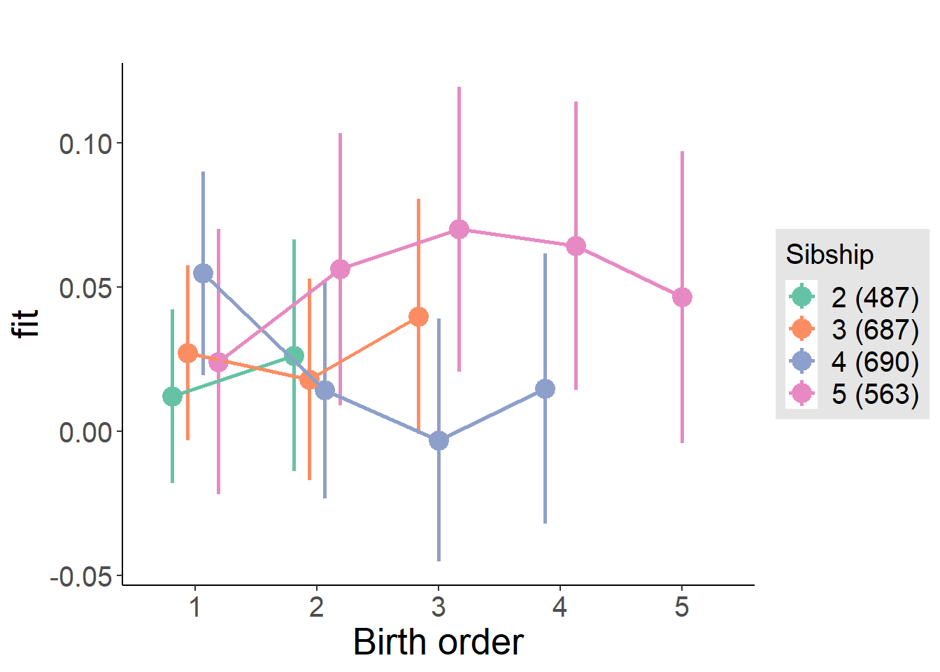
Model Comparison
###### Model 1 - Model 2
anova(m1_covariates_only, m2_birthorder_linear, m3_birthorder_nonlinear, m4_interaction)## refitting model(s) with ML (instead of REML)| Df | AIC | BIC | logLik | deviance | Chisq | Chi Df | Pr(>Chisq) |
|---|---|---|---|---|---|---|---|
| 10 | -1477 | -1419 | 748.3 | -1497 | NA | NA | NA |
| 11 | -1475 | -1411 | 748.4 | -1497 | 0.1035 | 1 | 0.7477 |
| 14 | -1469 | -1388 | 748.5 | -1497 | 0.2679 | 3 | 0.9659 |
| 20 | -1475 | -1359 | 757.5 | -1515 | 18.02 | 6 | 0.006178 |
Parental full sibling order
outcome_parental_m1 <- update(m2_birthorder_linear, data = birthorder %>%
mutate(sibling_count = sibling_count_genes_factor,
birth_order_nonlinear = birthorder_genes_factor,
birth_order = birthorder_genes,
count_birth_order = count_birthorder_genes
) %>%
filter(sibling_count != "1"))## boundary (singular) fit: see ?isSingularcompare_models_markdown(outcome_parental_m1)Basic Model
Model Summary
m1_covariates_only <- update(m2_birthorder_linear, formula = . ~ . - birth_order)## boundary (singular) fit: see ?isSingulartidy(m1_covariates_only, conf.int = T, conf.level = 0.995)| effect | group | term | estimate | std.error | statistic | df | p.value | conf.low | conf.high |
|---|---|---|---|---|---|---|---|---|---|
| fixed | NA | (Intercept) | 0.1656 | 0.1532 | 1.081 | 2638 | 0.2797 | -0.2643 | 0.5955 |
| fixed | NA | poly(age, 3, raw = TRUE)1 | -0.01208 | 0.017 | -0.7107 | 2638 | 0.4774 | -0.05979 | 0.03563 |
| fixed | NA | poly(age, 3, raw = TRUE)2 | 0.0003581 | 0.0006033 | 0.5936 | 2638 | 0.5529 | -0.001335 | 0.002052 |
| fixed | NA | poly(age, 3, raw = TRUE)3 | -0.000003593 | 0.000006861 | -0.5237 | 2638 | 0.6005 | -0.00002285 | 0.00001567 |
| fixed | NA | male | -0.01661 | 0.007146 | -2.324 | 2638 | 0.02018 | -0.03667 | 0.003449 |
| fixed | NA | sibling_count3 | 0.006755 | 0.009596 | 0.7039 | 2638 | 0.4816 | -0.02018 | 0.03369 |
| fixed | NA | sibling_count4 | 0.01013 | 0.01003 | 1.009 | 2638 | 0.3128 | -0.01803 | 0.03829 |
| fixed | NA | sibling_count5 | 0.03126 | 0.01142 | 2.738 | 2638 | 0.006224 | -0.000789 | 0.06331 |
| ran_pars | mother_pidlink | sd__(Intercept) | 0 | NA | NA | NA | NA | NA | NA |
| ran_pars | Residual | sd__Observation | 0.181 | NA | NA | NA | NA | NA | NA |
Coefficient Plot
plot(allEffects(m1_covariates_only, confidence.level = 0.995))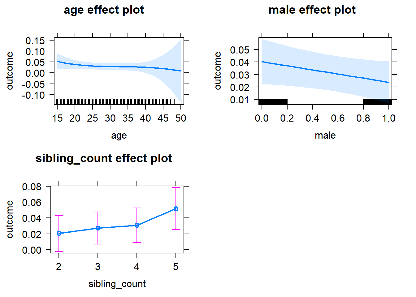
Add Birth Order Linear
Model Summary
tidy(m2_birthorder_linear, conf.int = T, conf.level = 0.995)| effect | group | term | estimate | std.error | statistic | df | p.value | conf.low | conf.high |
|---|---|---|---|---|---|---|---|---|---|
| fixed | NA | (Intercept) | 0.1671 | 0.1531 | 1.091 | 2637 | 0.2753 | -0.2627 | 0.5969 |
| fixed | NA | birth_order | -0.005689 | 0.00367 | -1.55 | 2637 | 0.1213 | -0.01599 | 0.004614 |
| fixed | NA | poly(age, 3, raw = TRUE)1 | -0.01157 | 0.01699 | -0.6808 | 2637 | 0.496 | -0.05927 | 0.03613 |
| fixed | NA | poly(age, 3, raw = TRUE)2 | 0.0003494 | 0.0006032 | 0.5793 | 2637 | 0.5625 | -0.001344 | 0.002043 |
| fixed | NA | poly(age, 3, raw = TRUE)3 | -0.000003631 | 0.000006859 | -0.5294 | 2637 | 0.5966 | -0.00002289 | 0.00001562 |
| fixed | NA | male | -0.01669 | 0.007144 | -2.336 | 2637 | 0.01955 | -0.03675 | 0.003363 |
| fixed | NA | sibling_count3 | 0.009469 | 0.009752 | 0.971 | 2637 | 0.3316 | -0.0179 | 0.03684 |
| fixed | NA | sibling_count4 | 0.01587 | 0.01069 | 1.484 | 2637 | 0.1379 | -0.01414 | 0.04588 |
| fixed | NA | sibling_count5 | 0.04055 | 0.01289 | 3.145 | 2637 | 0.001678 | 0.00436 | 0.07674 |
| ran_pars | mother_pidlink | sd__(Intercept) | 0 | NA | NA | NA | NA | NA | NA |
| ran_pars | Residual | sd__Observation | 0.181 | NA | NA | NA | NA | NA | NA |
Coefficient Plot
plot_birthorder2(m2_birthorder_linear, separate = FALSE)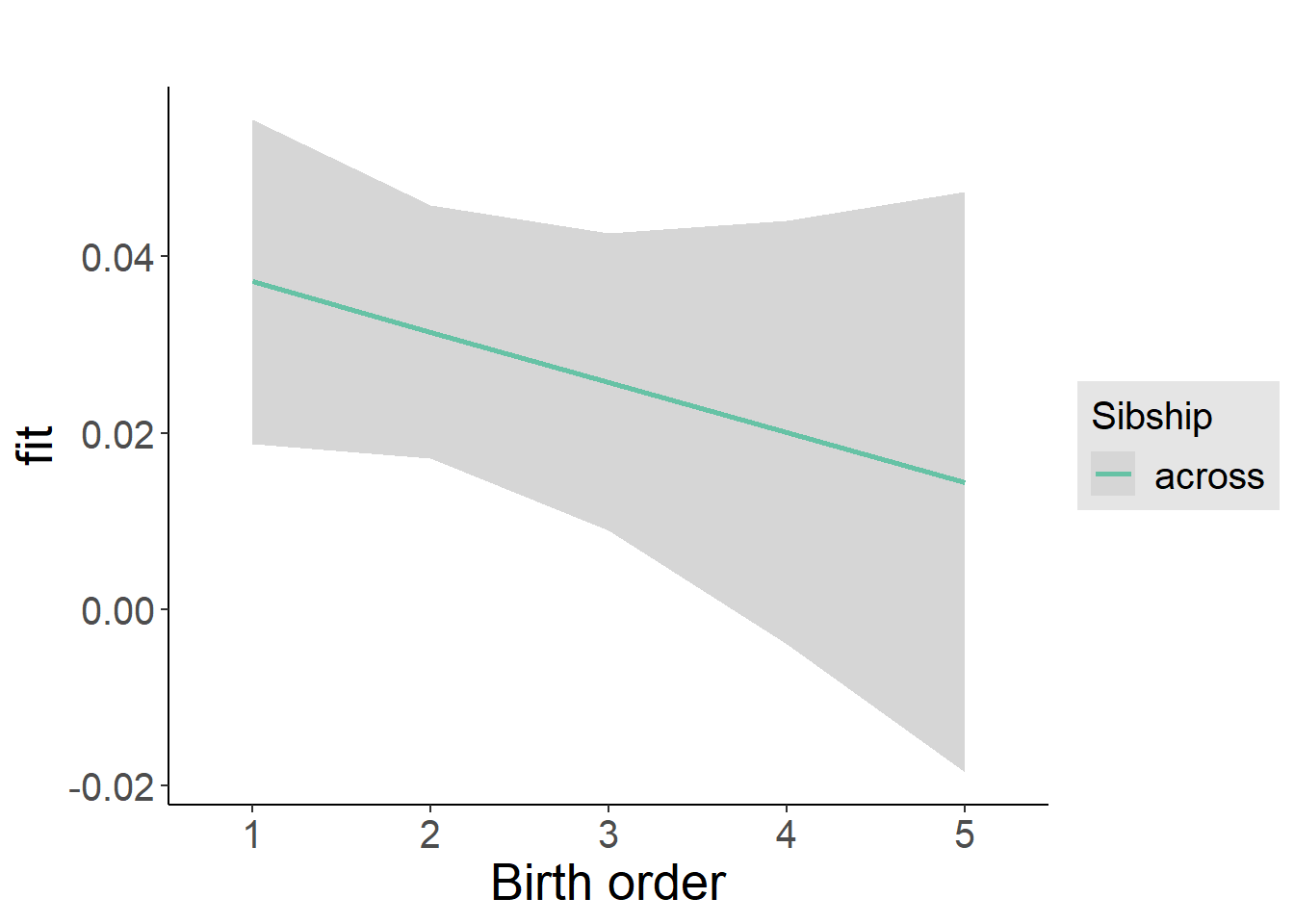
Add Birth Order Factor
Model Summary
m3_birthorder_nonlinear = update(m1_covariates_only, formula = . ~ . + birth_order_nonlinear)## boundary (singular) fit: see ?isSingulartidy(m3_birthorder_nonlinear, conf.int = T, conf.level = 0.995)| effect | group | term | estimate | std.error | statistic | df | p.value | conf.low | conf.high |
|---|---|---|---|---|---|---|---|---|---|
| fixed | NA | (Intercept) | 0.1558 | 0.1534 | 1.015 | 2634 | 0.3101 | -0.2749 | 0.5864 |
| fixed | NA | poly(age, 3, raw = TRUE)1 | -0.01093 | 0.01702 | -0.642 | 2634 | 0.5209 | -0.05872 | 0.03686 |
| fixed | NA | poly(age, 3, raw = TRUE)2 | 0.0003265 | 0.0006043 | 0.5404 | 2634 | 0.589 | -0.00137 | 0.002023 |
| fixed | NA | poly(age, 3, raw = TRUE)3 | -0.00000338 | 0.000006871 | -0.492 | 2634 | 0.6228 | -0.00002267 | 0.00001591 |
| fixed | NA | male | -0.01653 | 0.007152 | -2.311 | 2634 | 0.02091 | -0.0366 | 0.003547 |
| fixed | NA | sibling_count3 | 0.008106 | 0.009922 | 0.817 | 2634 | 0.414 | -0.01975 | 0.03596 |
| fixed | NA | sibling_count4 | 0.0152 | 0.01085 | 1.401 | 2634 | 0.1613 | -0.01526 | 0.04567 |
| fixed | NA | sibling_count5 | 0.04143 | 0.01312 | 3.157 | 2634 | 0.001612 | 0.004593 | 0.07826 |
| fixed | NA | birth_order_nonlinear2 | -0.005676 | 0.008611 | -0.6591 | 2634 | 0.5099 | -0.02985 | 0.0185 |
| fixed | NA | birth_order_nonlinear3 | -0.005663 | 0.01057 | -0.5358 | 2634 | 0.5921 | -0.03533 | 0.024 |
| fixed | NA | birth_order_nonlinear4 | -0.02034 | 0.01446 | -1.407 | 2634 | 0.1596 | -0.06094 | 0.02025 |
| fixed | NA | birth_order_nonlinear5 | -0.02933 | 0.02314 | -1.268 | 2634 | 0.205 | -0.09427 | 0.03561 |
| ran_pars | mother_pidlink | sd__(Intercept) | 0 | NA | NA | NA | NA | NA | NA |
| ran_pars | Residual | sd__Observation | 0.181 | NA | NA | NA | NA | NA | NA |
Coefficient Plot
plot_birthorder(m3_birthorder_nonlinear, separate = FALSE)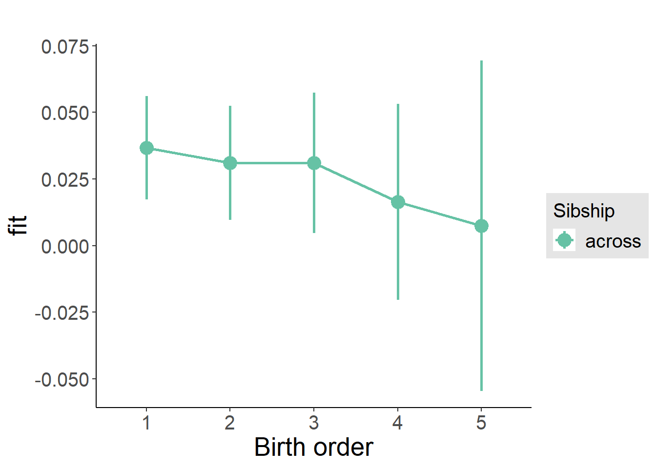
Add Interaction
Model Summary
m4_interaction = update(m3_birthorder_nonlinear, formula = . ~ . - birth_order_nonlinear - sibling_count + count_birth_order)## boundary (singular) fit: see ?isSingulartidy(m4_interaction, conf.int = T, conf.level = 0.995)| effect | group | term | estimate | std.error | statistic | df | p.value | conf.low | conf.high |
|---|---|---|---|---|---|---|---|---|---|
| fixed | NA | (Intercept) | 0.1514 | 0.1536 | 0.9857 | 2628 | 0.3244 | -0.2798 | 0.5826 |
| fixed | NA | poly(age, 3, raw = TRUE)1 | -0.0109 | 0.01705 | -0.6394 | 2628 | 0.5226 | -0.05875 | 0.03695 |
| fixed | NA | poly(age, 3, raw = TRUE)2 | 0.000327 | 0.0006051 | 0.5403 | 2628 | 0.589 | -0.001372 | 0.002026 |
| fixed | NA | poly(age, 3, raw = TRUE)3 | -0.000003406 | 0.000006882 | -0.4949 | 2628 | 0.6207 | -0.00002272 | 0.00001591 |
| fixed | NA | male | -0.01672 | 0.007163 | -2.335 | 2628 | 0.01962 | -0.03683 | 0.003381 |
| fixed | NA | count_birth_order2/2 | 0.006029 | 0.01544 | 0.3905 | 2628 | 0.6962 | -0.03731 | 0.04936 |
| fixed | NA | count_birth_order1/3 | 0.01013 | 0.0129 | 0.785 | 2628 | 0.4325 | -0.02608 | 0.04633 |
| fixed | NA | count_birth_order2/3 | 0.004701 | 0.01435 | 0.3277 | 2628 | 0.7432 | -0.03557 | 0.04498 |
| fixed | NA | count_birth_order3/3 | 0.01197 | 0.01547 | 0.7742 | 2628 | 0.4389 | -0.03144 | 0.05539 |
| fixed | NA | count_birth_order1/4 | 0.02871 | 0.01518 | 1.892 | 2628 | 0.05862 | -0.01389 | 0.07131 |
| fixed | NA | count_birth_order2/4 | 0.01124 | 0.01593 | 0.7059 | 2628 | 0.4803 | -0.03347 | 0.05596 |
| fixed | NA | count_birth_order3/4 | 0.001901 | 0.01654 | 0.115 | 2628 | 0.9085 | -0.04452 | 0.04832 |
| fixed | NA | count_birth_order4/4 | 0.0007442 | 0.01795 | 0.04147 | 2628 | 0.9669 | -0.04963 | 0.05112 |
| fixed | NA | count_birth_order1/5 | 0.04729 | 0.0199 | 2.377 | 2628 | 0.01755 | -0.008565 | 0.1031 |
| fixed | NA | count_birth_order2/5 | 0.0305 | 0.02218 | 1.375 | 2628 | 0.1693 | -0.03176 | 0.09276 |
| fixed | NA | count_birth_order3/5 | 0.0493 | 0.0216 | 2.282 | 2628 | 0.02254 | -0.01133 | 0.1099 |
| fixed | NA | count_birth_order4/5 | 0.02215 | 0.02078 | 1.066 | 2628 | 0.2866 | -0.03618 | 0.08047 |
| fixed | NA | count_birth_order5/5 | 0.016 | 0.02207 | 0.7251 | 2628 | 0.4685 | -0.04595 | 0.07795 |
| ran_pars | mother_pidlink | sd__(Intercept) | 0 | NA | NA | NA | NA | NA | NA |
| ran_pars | Residual | sd__Observation | 0.1812 | NA | NA | NA | NA | NA | NA |
Coefficient Plot
plot_birthorder(m4_interaction)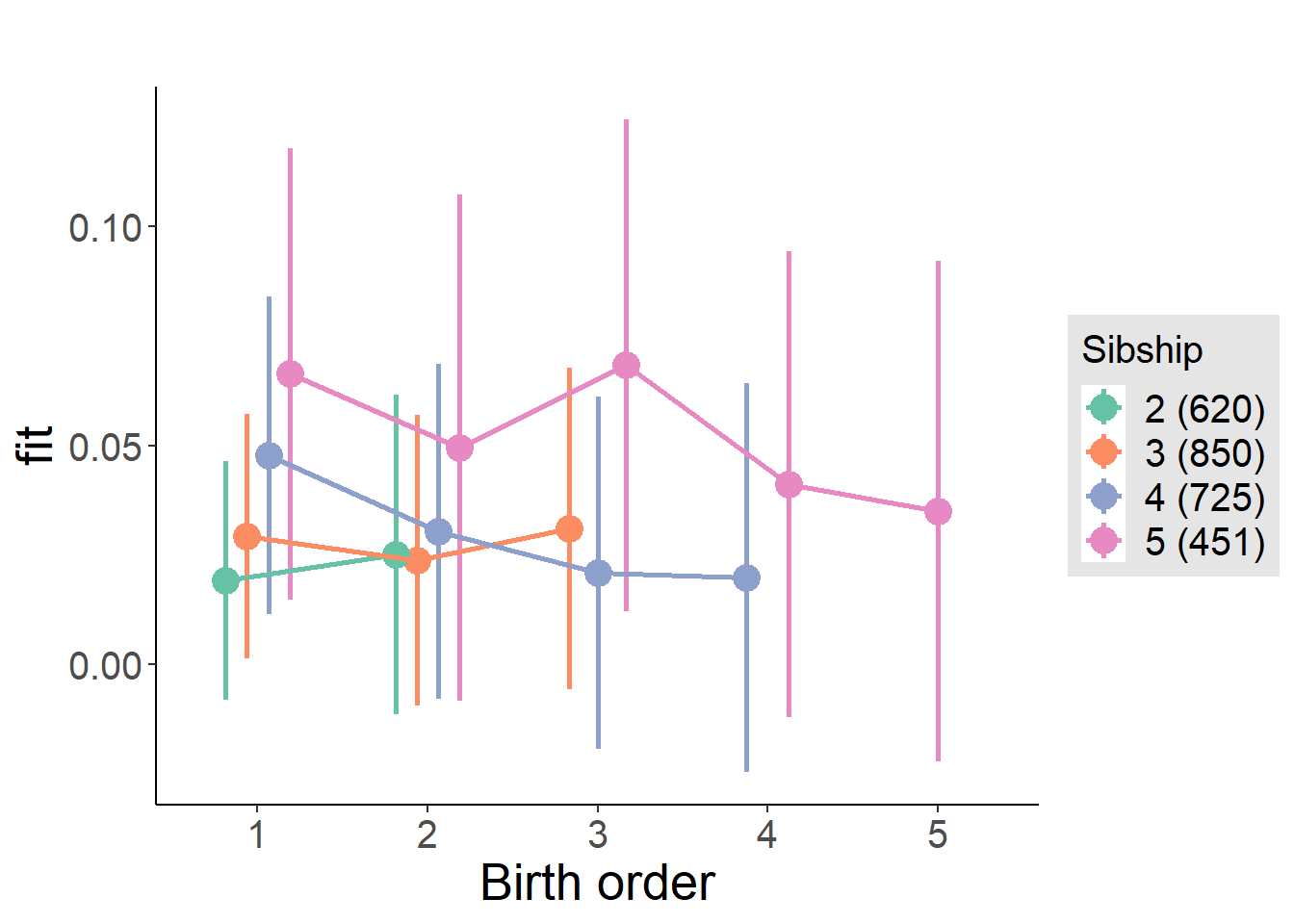
Model Comparison
###### Model 1 - Model 2
anova(m1_covariates_only, m2_birthorder_linear, m3_birthorder_nonlinear, m4_interaction)## refitting model(s) with ML (instead of REML)| Df | AIC | BIC | logLik | deviance | Chisq | Chi Df | Pr(>Chisq) |
|---|---|---|---|---|---|---|---|
| 10 | -1524 | -1466 | 772.2 | -1544 | NA | NA | NA |
| 11 | -1525 | -1460 | 773.4 | -1547 | 2.409 | 1 | 0.1206 |
| 14 | -1519 | -1437 | 773.6 | -1547 | 0.5734 | 3 | 0.9025 |
| 20 | -1510 | -1392 | 775 | -1550 | 2.717 | 6 | 0.8435 |
Compare birth order specifications
library(coefplot)
multiplot(outcome_naive_m1, outcome_preg_m1, outcome_uterus_m1, outcome_parental_m1, dodgeHeight = 0.6,
intercept = FALSE)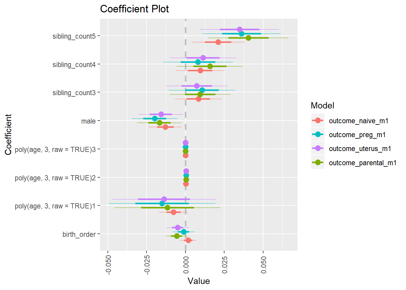
Smoking Behaviour
ever_smoked
birthorder <- birthorder %>% mutate(outcome = ever_smoked)
model = lmer(outcome ~ birth_order + poly(age, 3, raw = TRUE) + male + sibling_count + (1 | mother_pidlink),
data = birthorder)
compare_birthorder_specs(model)Naive birth order
outcome_naive_m1 <- update(m2_birthorder_linear, data = birthorder %>%
mutate(sibling_count = sibling_count_naive_factor,
birth_order_nonlinear = birthorder_naive_factor,
birth_order = birthorder_naive,
count_birth_order = count_birthorder_naive) %>%
filter(sibling_count != "1"))
compare_models_markdown(outcome_naive_m1)Basic Model
Model Summary
m1_covariates_only <- update(m2_birthorder_linear, formula = . ~ . - birth_order)
tidy(m1_covariates_only, conf.int = T, conf.level = 0.995)| effect | group | term | estimate | std.error | statistic | df | p.value | conf.low | conf.high |
|---|---|---|---|---|---|---|---|---|---|
| fixed | NA | (Intercept) | -1.01 | 0.06453 | -15.65 | 7307 | 2.377e-54 | -1.191 | -0.829 |
| fixed | NA | poly(age, 3, raw = TRUE)1 | 0.0818 | 0.006139 | 13.32 | 7210 | 4.944e-40 | 0.06457 | 0.09903 |
| fixed | NA | poly(age, 3, raw = TRUE)2 | -0.001932 | 0.0001772 | -10.9 | 7080 | 1.913e-27 | -0.002429 | -0.001434 |
| fixed | NA | poly(age, 3, raw = TRUE)3 | 0.00001445 | 0.000001586 | 9.112 | 6974 | 1.041e-19 | 0.000009999 | 0.0000189 |
| fixed | NA | male | 0.6104 | 0.007689 | 79.39 | 7358 | 0 | 0.5889 | 0.632 |
| fixed | NA | sibling_count3 | -0.008623 | 0.01125 | -0.7666 | 5083 | 0.4433 | -0.0402 | 0.02295 |
| fixed | NA | sibling_count4 | 0.0002562 | 0.01161 | 0.02207 | 4545 | 0.9824 | -0.03233 | 0.03284 |
| fixed | NA | sibling_count5 | 0.01052 | 0.01217 | 0.8645 | 4043 | 0.3874 | -0.02364 | 0.04469 |
| ran_pars | mother_pidlink | sd__(Intercept) | 0.1273 | NA | NA | NA | NA | NA | NA |
| ran_pars | Residual | sd__Observation | 0.312 | NA | NA | NA | NA | NA | NA |
Coefficient Plot
plot(allEffects(m1_covariates_only, confidence.level = 0.995))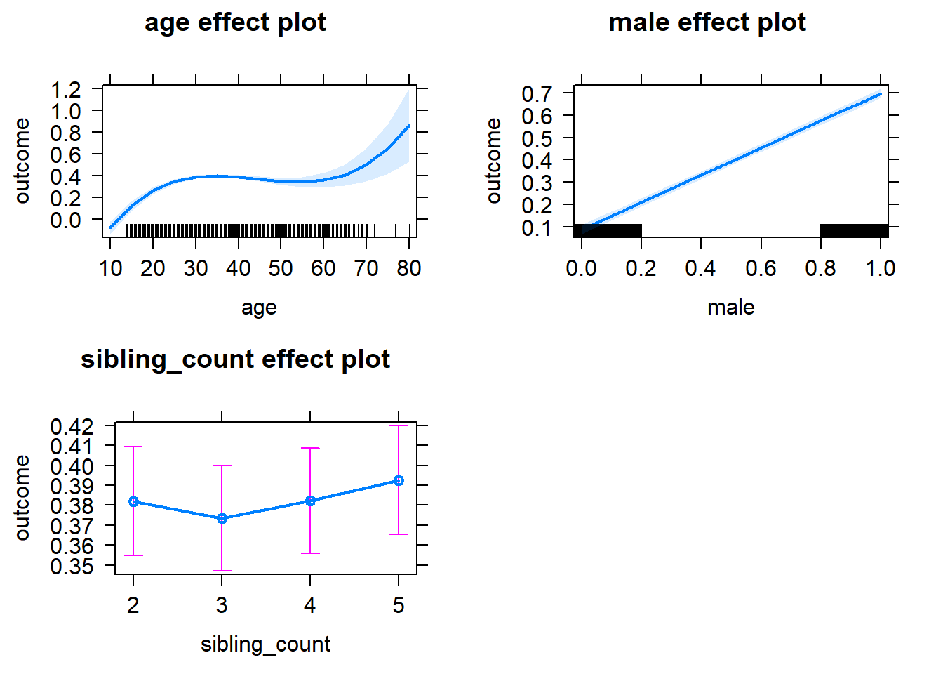
Add Birth Order Linear
Model Summary
tidy(m2_birthorder_linear, conf.int = T, conf.level = 0.995)| effect | group | term | estimate | std.error | statistic | df | p.value | conf.low | conf.high |
|---|---|---|---|---|---|---|---|---|---|
| fixed | NA | (Intercept) | -1.011 | 0.06455 | -15.66 | 7295 | 2.183e-54 | -1.192 | -0.8297 |
| fixed | NA | birth_order | 0.001735 | 0.003814 | 0.4549 | 6287 | 0.6492 | -0.008971 | 0.01244 |
| fixed | NA | poly(age, 3, raw = TRUE)1 | 0.08163 | 0.00615 | 13.27 | 7232 | 9.717e-40 | 0.06437 | 0.0989 |
| fixed | NA | poly(age, 3, raw = TRUE)2 | -0.001927 | 0.0001775 | -10.86 | 7093 | 3.005e-27 | -0.002426 | -0.001429 |
| fixed | NA | poly(age, 3, raw = TRUE)3 | 0.00001442 | 0.000001587 | 9.085 | 6981 | 1.324e-19 | 0.000009966 | 0.00001888 |
| fixed | NA | male | 0.6104 | 0.00769 | 79.37 | 7357 | 0 | 0.5888 | 0.632 |
| fixed | NA | sibling_count3 | -0.009235 | 0.01133 | -0.8152 | 5221 | 0.415 | -0.04103 | 0.02256 |
| fixed | NA | sibling_count4 | -0.001164 | 0.01202 | -0.09679 | 5097 | 0.9229 | -0.03491 | 0.03258 |
| fixed | NA | sibling_count5 | 0.008236 | 0.01317 | 0.6254 | 5123 | 0.5317 | -0.02873 | 0.0452 |
| ran_pars | mother_pidlink | sd__(Intercept) | 0.1273 | NA | NA | NA | NA | NA | NA |
| ran_pars | Residual | sd__Observation | 0.312 | NA | NA | NA | NA | NA | NA |
Coefficient Plot
plot_birthorder2(m2_birthorder_linear, separate = FALSE)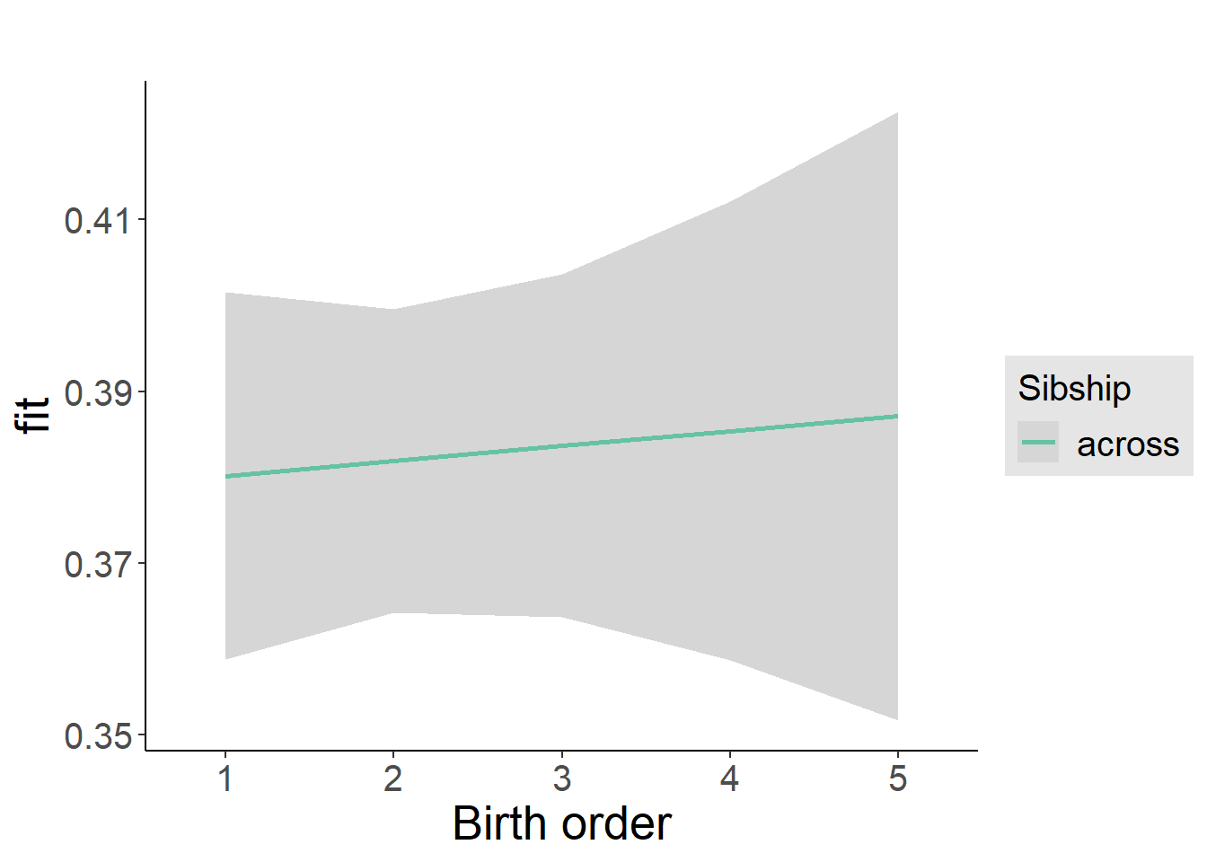
Add Birth Order Factor
Model Summary
m3_birthorder_nonlinear = update(m1_covariates_only, formula = . ~ . + birth_order_nonlinear)
tidy(m3_birthorder_nonlinear, conf.int = T, conf.level = 0.995)| effect | group | term | estimate | std.error | statistic | df | p.value | conf.low | conf.high |
|---|---|---|---|---|---|---|---|---|---|
| fixed | NA | (Intercept) | -1.011 | 0.0647 | -15.63 | 7315 | 3.422e-54 | -1.193 | -0.8296 |
| fixed | NA | poly(age, 3, raw = TRUE)1 | 0.08161 | 0.006152 | 13.26 | 7220 | 1.076e-39 | 0.06434 | 0.09888 |
| fixed | NA | poly(age, 3, raw = TRUE)2 | -0.00193 | 0.0001776 | -10.86 | 7072 | 2.793e-27 | -0.002428 | -0.001431 |
| fixed | NA | poly(age, 3, raw = TRUE)3 | 0.00001447 | 0.000001589 | 9.105 | 6948 | 1.105e-19 | 0.00001001 | 0.00001893 |
| fixed | NA | male | 0.6105 | 0.007689 | 79.39 | 7354 | 0 | 0.5889 | 0.6321 |
| fixed | NA | sibling_count3 | -0.007945 | 0.01149 | -0.6914 | 5453 | 0.4893 | -0.0402 | 0.02431 |
| fixed | NA | sibling_count4 | -0.003305 | 0.0122 | -0.2708 | 5348 | 0.7865 | -0.03755 | 0.03094 |
| fixed | NA | sibling_count5 | 0.01166 | 0.01328 | 0.8774 | 5301 | 0.3803 | -0.02563 | 0.04894 |
| fixed | NA | birth_order_nonlinear2 | 0.01073 | 0.009057 | 1.185 | 6131 | 0.236 | -0.01469 | 0.03616 |
| fixed | NA | birth_order_nonlinear3 | -0.00006619 | 0.01159 | -0.005712 | 6040 | 0.9954 | -0.03259 | 0.03246 |
| fixed | NA | birth_order_nonlinear4 | 0.02572 | 0.01516 | 1.696 | 6043 | 0.08992 | -0.01685 | 0.06828 |
| fixed | NA | birth_order_nonlinear5 | -0.02264 | 0.02226 | -1.017 | 5904 | 0.3092 | -0.08513 | 0.03985 |
| ran_pars | mother_pidlink | sd__(Intercept) | 0.1271 | NA | NA | NA | NA | NA | NA |
| ran_pars | Residual | sd__Observation | 0.312 | NA | NA | NA | NA | NA | NA |
Coefficient Plot
plot_birthorder(m3_birthorder_nonlinear, separate = FALSE)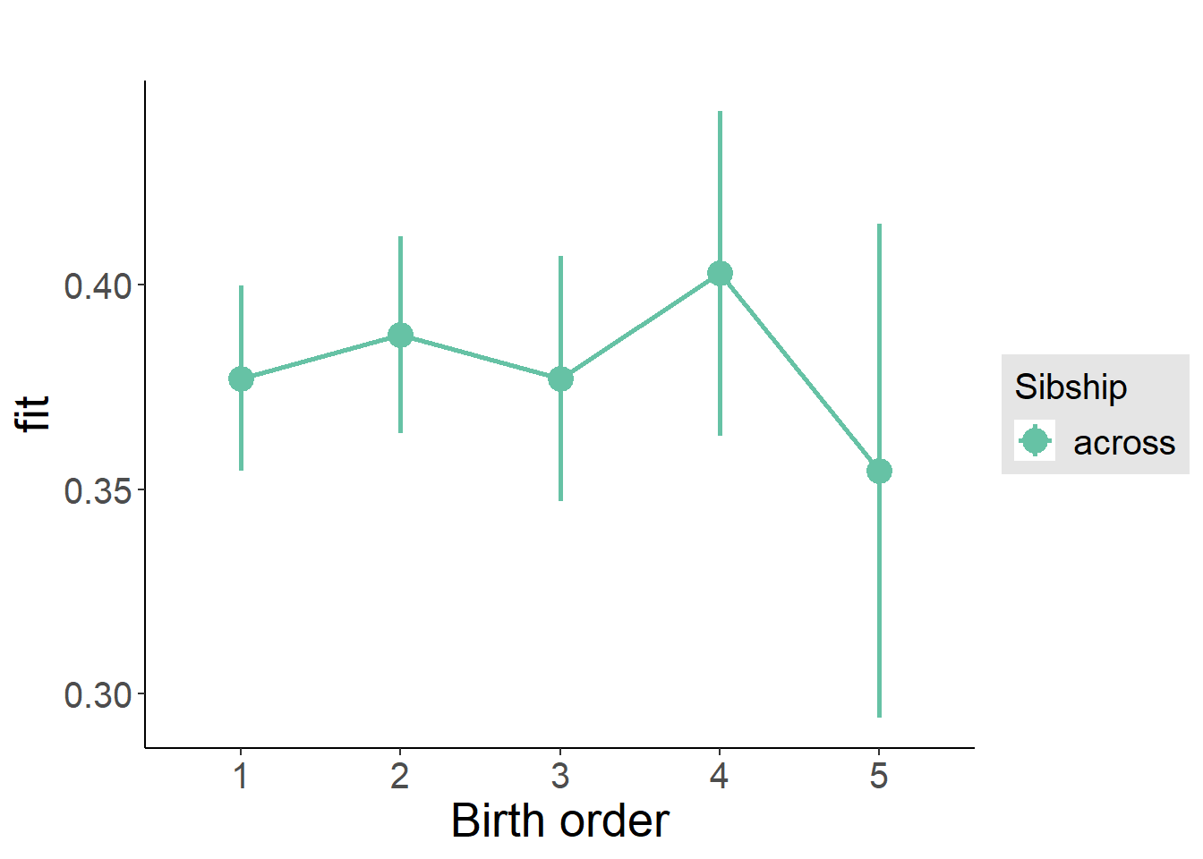
Add Interaction
Model Summary
m4_interaction = update(m3_birthorder_nonlinear, formula = . ~ . - birth_order_nonlinear - sibling_count + count_birth_order)
tidy(m4_interaction, conf.int = T, conf.level = 0.995)| effect | group | term | estimate | std.error | statistic | df | p.value | conf.low | conf.high |
|---|---|---|---|---|---|---|---|---|---|
| fixed | NA | (Intercept) | -1.015 | 0.06481 | -15.66 | 7318 | 2.079e-54 | -1.197 | -0.8331 |
| fixed | NA | poly(age, 3, raw = TRUE)1 | 0.08158 | 0.006151 | 13.26 | 7217 | 1.108e-39 | 0.06432 | 0.09885 |
| fixed | NA | poly(age, 3, raw = TRUE)2 | -0.001933 | 0.0001776 | -10.88 | 7066 | 2.289e-27 | -0.002431 | -0.001434 |
| fixed | NA | poly(age, 3, raw = TRUE)3 | 0.00001452 | 0.000001589 | 9.142 | 6939 | 7.947e-20 | 0.00001006 | 0.00001898 |
| fixed | NA | male | 0.6102 | 0.007689 | 79.35 | 7348 | 0 | 0.5886 | 0.6318 |
| fixed | NA | count_birth_order2/2 | 0.02546 | 0.01546 | 1.647 | 6092 | 0.09959 | -0.01793 | 0.06884 |
| fixed | NA | count_birth_order1/3 | -0.01326 | 0.01477 | -0.8972 | 7475 | 0.3696 | -0.05473 | 0.02821 |
| fixed | NA | count_birth_order2/3 | 0.01553 | 0.01651 | 0.9403 | 7511 | 0.3471 | -0.03082 | 0.06187 |
| fixed | NA | count_birth_order3/3 | 0.009555 | 0.01841 | 0.5191 | 7523 | 0.6037 | -0.04212 | 0.06123 |
| fixed | NA | count_birth_order1/4 | 0.01465 | 0.01672 | 0.8759 | 7512 | 0.3811 | -0.03229 | 0.06159 |
| fixed | NA | count_birth_order2/4 | 0.007809 | 0.01778 | 0.4392 | 7521 | 0.6605 | -0.0421 | 0.05772 |
| fixed | NA | count_birth_order3/4 | 0.0003214 | 0.01929 | 0.01666 | 7520 | 0.9867 | -0.05382 | 0.05447 |
| fixed | NA | count_birth_order4/4 | 0.01523 | 0.02023 | 0.7526 | 7514 | 0.4517 | -0.04157 | 0.07202 |
| fixed | NA | count_birth_order1/5 | 0.0381 | 0.01915 | 1.99 | 7523 | 0.04663 | -0.01564 | 0.09184 |
| fixed | NA | count_birth_order2/5 | 0.004619 | 0.02023 | 0.2284 | 7515 | 0.8194 | -0.05215 | 0.06139 |
| fixed | NA | count_birth_order3/5 | 0.003229 | 0.02065 | 0.1564 | 7509 | 0.8757 | -0.05473 | 0.06119 |
| fixed | NA | count_birth_order4/5 | 0.05861 | 0.02212 | 2.65 | 7483 | 0.008066 | -0.003473 | 0.1207 |
| fixed | NA | count_birth_order5/5 | -0.005772 | 0.02254 | -0.2561 | 7478 | 0.7979 | -0.06904 | 0.05749 |
| ran_pars | mother_pidlink | sd__(Intercept) | 0.1268 | NA | NA | NA | NA | NA | NA |
| ran_pars | Residual | sd__Observation | 0.3121 | NA | NA | NA | NA | NA | NA |
Coefficient Plot
plot_birthorder(m4_interaction)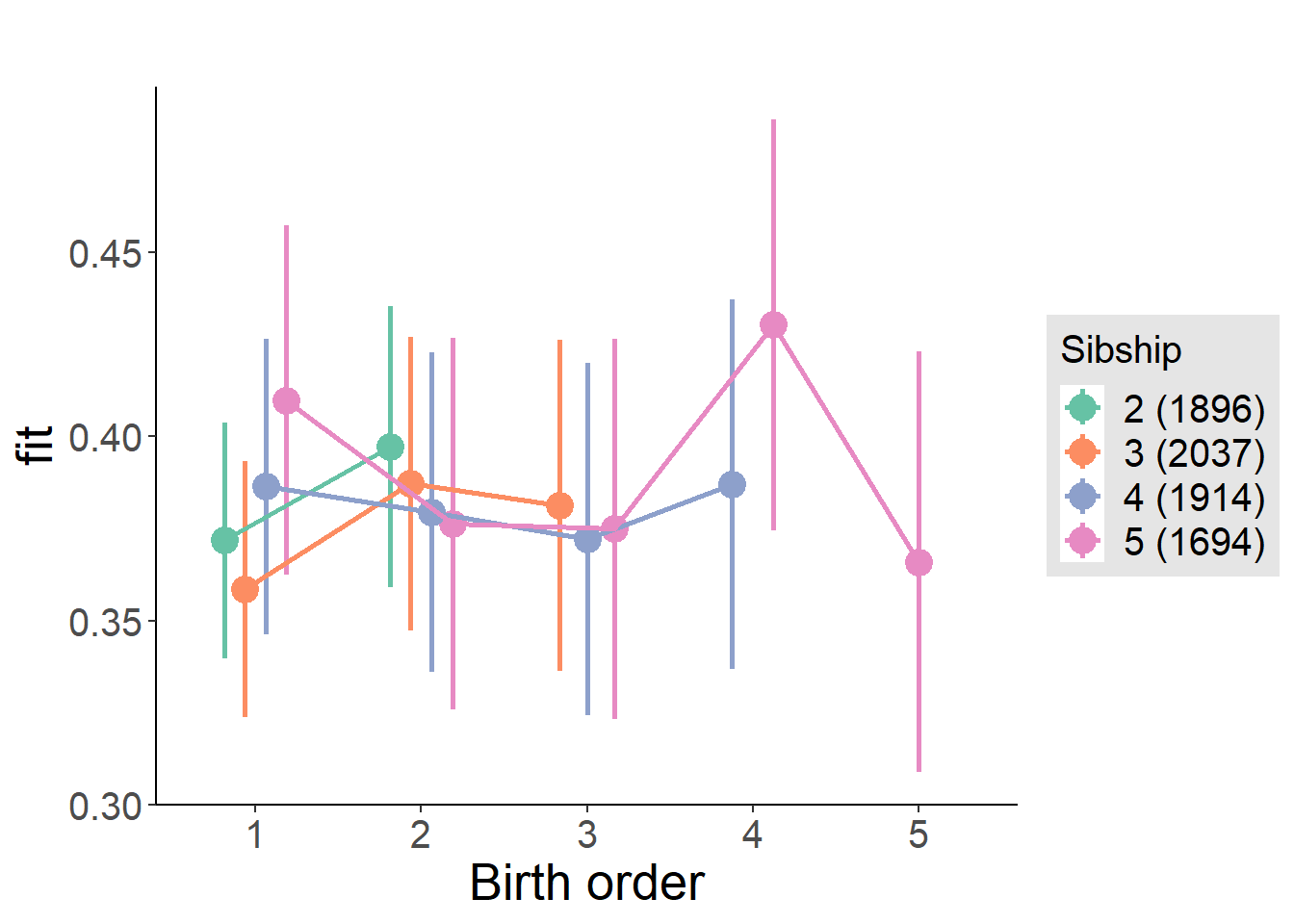
Model Comparison
###### Model 1 - Model 2
anova(m1_covariates_only, m2_birthorder_linear, m3_birthorder_nonlinear, m4_interaction)## refitting model(s) with ML (instead of REML)| Df | AIC | BIC | logLik | deviance | Chisq | Chi Df | Pr(>Chisq) |
|---|---|---|---|---|---|---|---|
| 10 | 4935 | 5005 | -2458 | 4915 | NA | NA | NA |
| 11 | 4937 | 5013 | -2458 | 4915 | 0.2072 | 1 | 0.649 |
| 14 | 4937 | 5034 | -2455 | 4909 | 5.918 | 3 | 0.1157 |
| 20 | 4940 | 5078 | -2450 | 4900 | 9.404 | 6 | 0.1521 |
Maternal birth order
outcome_uterus_m1 <- update(m2_birthorder_linear, data = birthorder %>%
mutate(sibling_count = sibling_count_uterus_alive_factor,
birth_order_nonlinear = birthorder_uterus_alive_factor,
birth_order = birthorder_uterus_alive,
count_birth_order = count_birthorder_uterus_alive) %>%
filter(sibling_count != "1"))
compare_models_markdown(outcome_uterus_m1)Basic Model
Model Summary
m1_covariates_only <- update(m2_birthorder_linear, formula = . ~ . - birth_order)
tidy(m1_covariates_only, conf.int = T, conf.level = 0.995)| effect | group | term | estimate | std.error | statistic | df | p.value | conf.low | conf.high |
|---|---|---|---|---|---|---|---|---|---|
| fixed | NA | (Intercept) | -1.65 | 0.1851 | -8.914 | 4718 | 6.901e-19 | -2.169 | -1.13 |
| fixed | NA | poly(age, 3, raw = TRUE)1 | 0.1578 | 0.02162 | 7.3 | 4724 | 3.364e-13 | 0.09712 | 0.2185 |
| fixed | NA | poly(age, 3, raw = TRUE)2 | -0.00466 | 0.0007975 | -5.843 | 4728 | 0.000000005481 | -0.006898 | -0.002421 |
| fixed | NA | poly(age, 3, raw = TRUE)3 | 0.00004461 | 0.000009355 | 4.768 | 4731 | 0.000001917 | 0.00001835 | 0.00007087 |
| fixed | NA | male | 0.5543 | 0.009918 | 55.88 | 4617 | 0 | 0.5264 | 0.5821 |
| fixed | NA | sibling_count3 | 0.008032 | 0.01375 | 0.584 | 3405 | 0.5593 | -0.03058 | 0.04664 |
| fixed | NA | sibling_count4 | 0.005352 | 0.01489 | 0.3596 | 2997 | 0.7192 | -0.03643 | 0.04714 |
| fixed | NA | sibling_count5 | 0.03346 | 0.01715 | 1.95 | 2679 | 0.05122 | -0.01469 | 0.08161 |
| ran_pars | mother_pidlink | sd__(Intercept) | 0.1376 | NA | NA | NA | NA | NA | NA |
| ran_pars | Residual | sd__Observation | 0.3162 | NA | NA | NA | NA | NA | NA |
Coefficient Plot
plot(allEffects(m1_covariates_only, confidence.level = 0.995))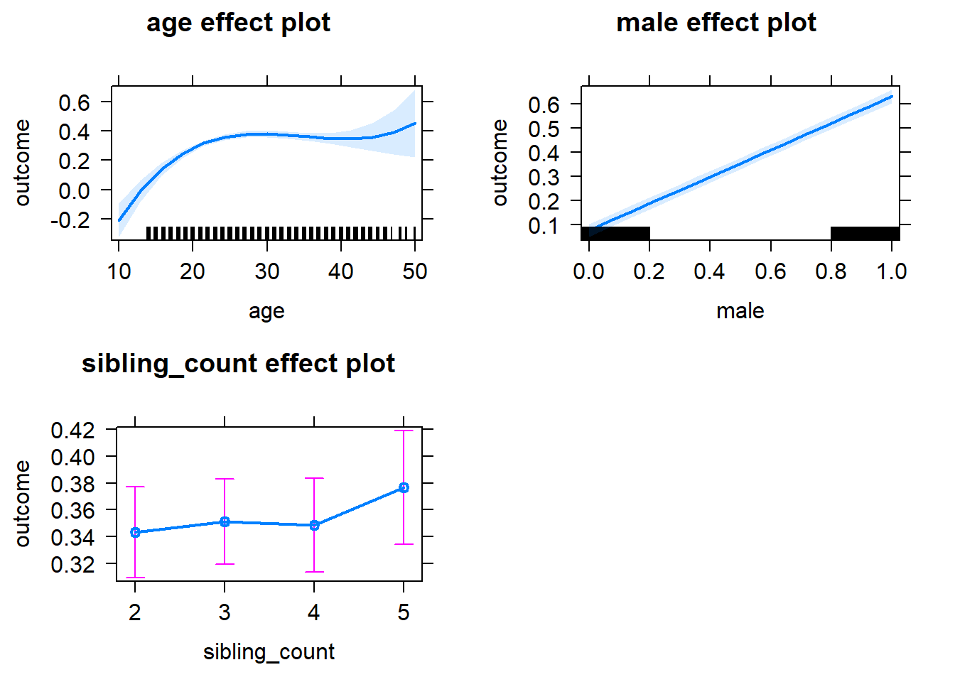
Add Birth Order Linear
Model Summary
tidy(m2_birthorder_linear, conf.int = T, conf.level = 0.995)| effect | group | term | estimate | std.error | statistic | df | p.value | conf.low | conf.high |
|---|---|---|---|---|---|---|---|---|---|
| fixed | NA | (Intercept) | -1.654 | 0.1853 | -8.927 | 4718 | 6.177e-19 | -2.175 | -1.134 |
| fixed | NA | birth_order | 0.002531 | 0.005204 | 0.4864 | 4335 | 0.6267 | -0.01208 | 0.01714 |
| fixed | NA | poly(age, 3, raw = TRUE)1 | 0.158 | 0.02162 | 7.306 | 4723 | 3.205e-13 | 0.09729 | 0.2187 |
| fixed | NA | poly(age, 3, raw = TRUE)2 | -0.004669 | 0.0007978 | -5.852 | 4727 | 0.000000005187 | -0.006908 | -0.002429 |
| fixed | NA | poly(age, 3, raw = TRUE)3 | 0.00004476 | 0.000009362 | 4.782 | 4730 | 0.000001793 | 0.00001848 | 0.00007104 |
| fixed | NA | male | 0.5542 | 0.009921 | 55.86 | 4616 | 0 | 0.5264 | 0.582 |
| fixed | NA | sibling_count3 | 0.006841 | 0.01397 | 0.4896 | 3471 | 0.6244 | -0.03238 | 0.04606 |
| fixed | NA | sibling_count4 | 0.002657 | 0.01588 | 0.1673 | 3228 | 0.8672 | -0.04193 | 0.04724 |
| fixed | NA | sibling_count5 | 0.02899 | 0.01946 | 1.49 | 3208 | 0.1363 | -0.02562 | 0.08361 |
| ran_pars | mother_pidlink | sd__(Intercept) | 0.1376 | NA | NA | NA | NA | NA | NA |
| ran_pars | Residual | sd__Observation | 0.3162 | NA | NA | NA | NA | NA | NA |
Coefficient Plot
plot_birthorder2(m2_birthorder_linear, separate = FALSE)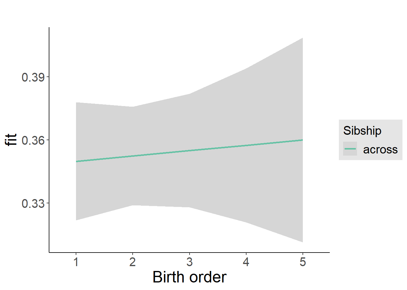
Add Birth Order Factor
Model Summary
m3_birthorder_nonlinear = update(m1_covariates_only, formula = . ~ . + birth_order_nonlinear)
tidy(m3_birthorder_nonlinear, conf.int = T, conf.level = 0.995)| effect | group | term | estimate | std.error | statistic | df | p.value | conf.low | conf.high |
|---|---|---|---|---|---|---|---|---|---|
| fixed | NA | (Intercept) | -1.672 | 0.1856 | -9.009 | 4721 | 2.95e-19 | -2.194 | -1.151 |
| fixed | NA | poly(age, 3, raw = TRUE)1 | 0.1598 | 0.02166 | 7.38 | 4724 | 1.855e-13 | 0.09905 | 0.2206 |
| fixed | NA | poly(age, 3, raw = TRUE)2 | -0.004735 | 0.000799 | -5.926 | 4727 | 0.000000003326 | -0.006978 | -0.002492 |
| fixed | NA | poly(age, 3, raw = TRUE)3 | 0.00004548 | 0.000009374 | 4.851 | 4728 | 0.000001265 | 0.00001916 | 0.00007179 |
| fixed | NA | male | 0.5544 | 0.009924 | 55.87 | 4614 | 0 | 0.5266 | 0.5823 |
| fixed | NA | sibling_count3 | 0.004789 | 0.01418 | 0.3379 | 3597 | 0.7355 | -0.035 | 0.04458 |
| fixed | NA | sibling_count4 | 0.00303 | 0.0161 | 0.1882 | 3335 | 0.8507 | -0.04216 | 0.04822 |
| fixed | NA | sibling_count5 | 0.03381 | 0.01977 | 1.71 | 3313 | 0.08734 | -0.02168 | 0.0893 |
| fixed | NA | birth_order_nonlinear2 | 0.01646 | 0.0117 | 1.407 | 3702 | 0.1596 | -0.01639 | 0.0493 |
| fixed | NA | birth_order_nonlinear3 | 0.0149 | 0.01496 | 0.996 | 3950 | 0.3193 | -0.02709 | 0.05689 |
| fixed | NA | birth_order_nonlinear4 | 0.0003706 | 0.02023 | 0.01832 | 4147 | 0.9854 | -0.05641 | 0.05715 |
| fixed | NA | birth_order_nonlinear5 | -0.003738 | 0.03166 | -0.1181 | 3948 | 0.906 | -0.09262 | 0.08514 |
| ran_pars | mother_pidlink | sd__(Intercept) | 0.137 | NA | NA | NA | NA | NA | NA |
| ran_pars | Residual | sd__Observation | 0.3165 | NA | NA | NA | NA | NA | NA |
Coefficient Plot
plot_birthorder(m3_birthorder_nonlinear, separate = FALSE)
Add Interaction
Model Summary
m4_interaction = update(m3_birthorder_nonlinear, formula = . ~ . - birth_order_nonlinear - sibling_count + count_birth_order)
tidy(m4_interaction, conf.int = T, conf.level = 0.995)| effect | group | term | estimate | std.error | statistic | df | p.value | conf.low | conf.high |
|---|---|---|---|---|---|---|---|---|---|
| fixed | NA | (Intercept) | -1.675 | 0.1857 | -9.016 | 4715 | 2.781e-19 | -2.196 | -1.153 |
| fixed | NA | poly(age, 3, raw = TRUE)1 | 0.1594 | 0.02167 | 7.357 | 4717 | 2.206e-13 | 0.09859 | 0.2202 |
| fixed | NA | poly(age, 3, raw = TRUE)2 | -0.004725 | 0.0007995 | -5.91 | 4720 | 0.00000000367 | -0.006969 | -0.002481 |
| fixed | NA | poly(age, 3, raw = TRUE)3 | 0.00004542 | 0.000009382 | 4.842 | 4722 | 0.000001329 | 0.00001909 | 0.00007176 |
| fixed | NA | male | 0.5543 | 0.009931 | 55.82 | 4608 | 0 | 0.5265 | 0.5822 |
| fixed | NA | count_birth_order2/2 | 0.0373 | 0.02004 | 1.861 | 3898 | 0.06277 | -0.01895 | 0.09354 |
| fixed | NA | count_birth_order1/3 | 0.02359 | 0.01802 | 1.309 | 4703 | 0.1906 | -0.02699 | 0.07416 |
| fixed | NA | count_birth_order2/3 | 0.01814 | 0.01957 | 0.9267 | 4721 | 0.3541 | -0.0368 | 0.07308 |
| fixed | NA | count_birth_order3/3 | 0.01768 | 0.02184 | 0.8094 | 4717 | 0.4183 | -0.04363 | 0.07898 |
| fixed | NA | count_birth_order1/4 | 0.005862 | 0.022 | 0.2664 | 4717 | 0.79 | -0.05591 | 0.06763 |
| fixed | NA | count_birth_order2/4 | 0.02353 | 0.02269 | 1.037 | 4721 | 0.2999 | -0.04018 | 0.08723 |
| fixed | NA | count_birth_order3/4 | 0.03487 | 0.024 | 1.453 | 4701 | 0.1463 | -0.0325 | 0.1022 |
| fixed | NA | count_birth_order4/4 | 0.009375 | 0.02492 | 0.3762 | 4697 | 0.7068 | -0.06058 | 0.07933 |
| fixed | NA | count_birth_order1/5 | 0.03575 | 0.02996 | 1.193 | 4716 | 0.2328 | -0.04835 | 0.1199 |
| fixed | NA | count_birth_order2/5 | 0.05873 | 0.0321 | 1.829 | 4671 | 0.06739 | -0.03138 | 0.1488 |
| fixed | NA | count_birth_order3/5 | 0.05768 | 0.02984 | 1.933 | 4677 | 0.05331 | -0.02609 | 0.1415 |
| fixed | NA | count_birth_order4/5 | 0.04303 | 0.02924 | 1.472 | 4685 | 0.1412 | -0.03905 | 0.1251 |
| fixed | NA | count_birth_order5/5 | 0.03718 | 0.03031 | 1.227 | 4663 | 0.2199 | -0.04789 | 0.1223 |
| ran_pars | mother_pidlink | sd__(Intercept) | 0.1368 | NA | NA | NA | NA | NA | NA |
| ran_pars | Residual | sd__Observation | 0.3167 | NA | NA | NA | NA | NA | NA |
Coefficient Plot
plot_birthorder(m4_interaction)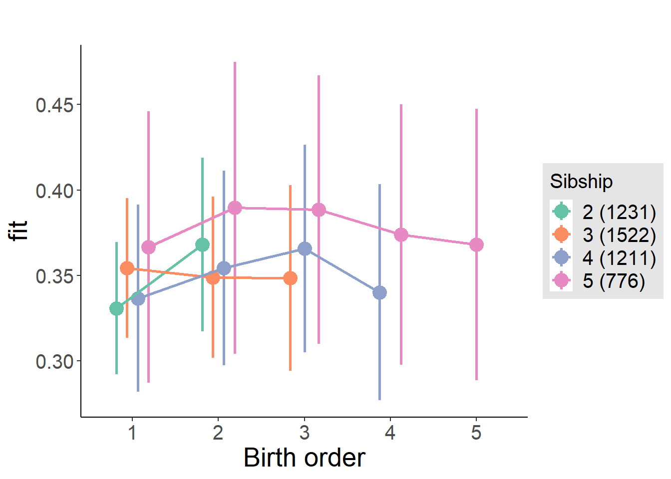
Model Comparison
###### Model 1 - Model 2
anova(m1_covariates_only, m2_birthorder_linear, m3_birthorder_nonlinear, m4_interaction)## refitting model(s) with ML (instead of REML)| Df | AIC | BIC | logLik | deviance | Chisq | Chi Df | Pr(>Chisq) |
|---|---|---|---|---|---|---|---|
| 10 | 3323 | 3388 | -1652 | 3303 | NA | NA | NA |
| 11 | 3325 | 3396 | -1651 | 3303 | 0.2371 | 1 | 0.6263 |
| 14 | 3328 | 3419 | -1650 | 3300 | 2.435 | 3 | 0.4871 |
| 20 | 3337 | 3467 | -1649 | 3297 | 3.029 | 6 | 0.8052 |
Maternal pregnancy order
outcome_preg_m1 <- update(m2_birthorder_linear, data = birthorder %>%
mutate(sibling_count = sibling_count_uterus_preg_factor,
birth_order_nonlinear = birthorder_uterus_preg_factor,
birth_order = birthorder_uterus_preg,
count_birth_order = count_birthorder_uterus_preg
) %>%
filter(sibling_count != "1"))
compare_models_markdown(outcome_preg_m1)Basic Model
Model Summary
m1_covariates_only <- update(m2_birthorder_linear, formula = . ~ . - birth_order)
tidy(m1_covariates_only, conf.int = T, conf.level = 0.995)| effect | group | term | estimate | std.error | statistic | df | p.value | conf.low | conf.high |
|---|---|---|---|---|---|---|---|---|---|
| fixed | NA | (Intercept) | -1.604 | 0.191 | -8.399 | 4378 | 6.019e-17 | -2.14 | -1.068 |
| fixed | NA | poly(age, 3, raw = TRUE)1 | 0.1527 | 0.02233 | 6.836 | 4383 | 9.256e-12 | 0.08997 | 0.2153 |
| fixed | NA | poly(age, 3, raw = TRUE)2 | -0.004458 | 0.0008243 | -5.408 | 4388 | 0.00000006696 | -0.006772 | -0.002144 |
| fixed | NA | poly(age, 3, raw = TRUE)3 | 0.00004212 | 0.000009672 | 4.355 | 4391 | 0.0000136 | 0.00001497 | 0.00006927 |
| fixed | NA | male | 0.5479 | 0.01032 | 53.08 | 4279 | 0 | 0.5189 | 0.5769 |
| fixed | NA | sibling_count3 | 0.009907 | 0.01493 | 0.6634 | 3256 | 0.5071 | -0.03201 | 0.05183 |
| fixed | NA | sibling_count4 | -0.00009172 | 0.0158 | -0.005807 | 2955 | 0.9954 | -0.04443 | 0.04425 |
| fixed | NA | sibling_count5 | 0.02209 | 0.01703 | 1.297 | 2677 | 0.1948 | -0.02572 | 0.0699 |
| ran_pars | mother_pidlink | sd__(Intercept) | 0.1393 | NA | NA | NA | NA | NA | NA |
| ran_pars | Residual | sd__Observation | 0.3162 | NA | NA | NA | NA | NA | NA |
Coefficient Plot
plot(allEffects(m1_covariates_only, confidence.level = 0.995))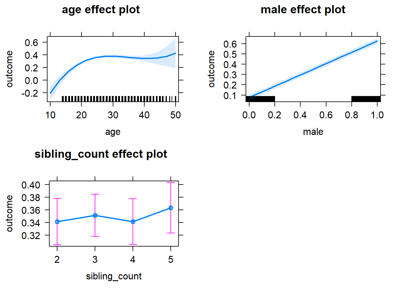
Add Birth Order Linear
Model Summary
tidy(m2_birthorder_linear, conf.int = T, conf.level = 0.995)| effect | group | term | estimate | std.error | statistic | df | p.value | conf.low | conf.high |
|---|---|---|---|---|---|---|---|---|---|
| fixed | NA | (Intercept) | -1.605 | 0.1912 | -8.391 | 4377 | 6.441e-17 | -2.141 | -1.068 |
| fixed | NA | birth_order | 0.0002651 | 0.00522 | 0.05079 | 4112 | 0.9595 | -0.01439 | 0.01492 |
| fixed | NA | poly(age, 3, raw = TRUE)1 | 0.1527 | 0.02234 | 6.835 | 4382 | 9.302e-12 | 0.08997 | 0.2154 |
| fixed | NA | poly(age, 3, raw = TRUE)2 | -0.004459 | 0.0008245 | -5.408 | 4387 | 0.00000006719 | -0.006773 | -0.002144 |
| fixed | NA | poly(age, 3, raw = TRUE)3 | 0.00004214 | 0.000009677 | 4.354 | 4390 | 0.00001365 | 0.00001497 | 0.0000693 |
| fixed | NA | male | 0.5479 | 0.01032 | 53.07 | 4278 | 0 | 0.5189 | 0.5769 |
| fixed | NA | sibling_count3 | 0.009783 | 0.01513 | 0.6465 | 3300 | 0.518 | -0.0327 | 0.05226 |
| fixed | NA | sibling_count4 | -0.0003638 | 0.01668 | -0.02181 | 3121 | 0.9826 | -0.04718 | 0.04646 |
| fixed | NA | sibling_count5 | 0.02166 | 0.01905 | 1.137 | 3065 | 0.2556 | -0.0318 | 0.07512 |
| ran_pars | mother_pidlink | sd__(Intercept) | 0.1393 | NA | NA | NA | NA | NA | NA |
| ran_pars | Residual | sd__Observation | 0.3163 | NA | NA | NA | NA | NA | NA |
Coefficient Plot
plot_birthorder2(m2_birthorder_linear, separate = FALSE)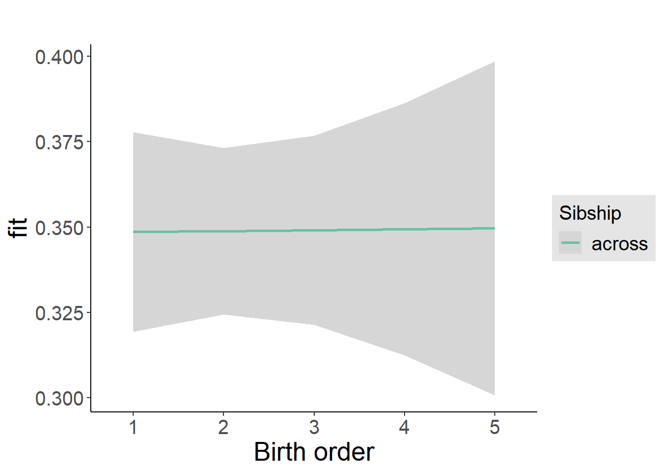
Add Birth Order Factor
Model Summary
m3_birthorder_nonlinear = update(m1_covariates_only, formula = . ~ . + birth_order_nonlinear)
tidy(m3_birthorder_nonlinear, conf.int = T, conf.level = 0.995)| effect | group | term | estimate | std.error | statistic | df | p.value | conf.low | conf.high |
|---|---|---|---|---|---|---|---|---|---|
| fixed | NA | (Intercept) | -1.62 | 0.1915 | -8.459 | 4381 | 3.624e-17 | -2.158 | -1.083 |
| fixed | NA | poly(age, 3, raw = TRUE)1 | 0.1539 | 0.02237 | 6.88 | 4384 | 6.839e-12 | 0.09111 | 0.2167 |
| fixed | NA | poly(age, 3, raw = TRUE)2 | -0.004503 | 0.0008257 | -5.453 | 4386 | 0.00000005217 | -0.006821 | -0.002185 |
| fixed | NA | poly(age, 3, raw = TRUE)3 | 0.00004262 | 0.000009689 | 4.398 | 4388 | 0.00001118 | 0.00001542 | 0.00006981 |
| fixed | NA | male | 0.5482 | 0.01033 | 53.09 | 4275 | 0 | 0.5192 | 0.5772 |
| fixed | NA | sibling_count3 | 0.009929 | 0.01535 | 0.6471 | 3407 | 0.5176 | -0.03314 | 0.053 |
| fixed | NA | sibling_count4 | 0.001297 | 0.0169 | 0.07672 | 3216 | 0.9389 | -0.04614 | 0.04874 |
| fixed | NA | sibling_count5 | 0.02456 | 0.01924 | 1.277 | 3118 | 0.2018 | -0.02944 | 0.07857 |
| fixed | NA | birth_order_nonlinear2 | 0.01625 | 0.01221 | 1.331 | 3483 | 0.1834 | -0.01803 | 0.05053 |
| fixed | NA | birth_order_nonlinear3 | 0.0009867 | 0.01547 | 0.06379 | 3729 | 0.9491 | -0.04243 | 0.0444 |
| fixed | NA | birth_order_nonlinear4 | -0.00312 | 0.02062 | -0.1513 | 3894 | 0.8797 | -0.06101 | 0.05477 |
| fixed | NA | birth_order_nonlinear5 | 0.002301 | 0.03024 | 0.07609 | 3774 | 0.9394 | -0.08258 | 0.08718 |
| ran_pars | mother_pidlink | sd__(Intercept) | 0.1391 | NA | NA | NA | NA | NA | NA |
| ran_pars | Residual | sd__Observation | 0.3164 | NA | NA | NA | NA | NA | NA |
Coefficient Plot
plot_birthorder(m3_birthorder_nonlinear, separate = FALSE)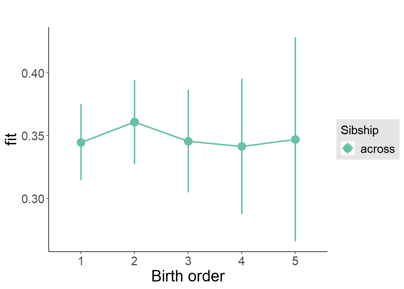
Add Interaction
Model Summary
m4_interaction = update(m3_birthorder_nonlinear, formula = . ~ . - birth_order_nonlinear - sibling_count + count_birth_order)
tidy(m4_interaction, conf.int = T, conf.level = 0.995)| effect | group | term | estimate | std.error | statistic | df | p.value | conf.low | conf.high |
|---|---|---|---|---|---|---|---|---|---|
| fixed | NA | (Intercept) | -1.627 | 0.1917 | -8.489 | 4375 | 2.819e-17 | -2.166 | -1.089 |
| fixed | NA | poly(age, 3, raw = TRUE)1 | 0.1537 | 0.02238 | 6.865 | 4377 | 7.565e-12 | 0.09083 | 0.2165 |
| fixed | NA | poly(age, 3, raw = TRUE)2 | -0.004488 | 0.0008263 | -5.432 | 4380 | 0.00000005868 | -0.006808 | -0.002169 |
| fixed | NA | poly(age, 3, raw = TRUE)3 | 0.00004236 | 0.000009697 | 4.369 | 4382 | 0.00001279 | 0.00001514 | 0.00006958 |
| fixed | NA | male | 0.5476 | 0.01033 | 52.99 | 4269 | 0 | 0.5186 | 0.5766 |
| fixed | NA | count_birth_order2/2 | 0.04198 | 0.02202 | 1.907 | 3681 | 0.05666 | -0.01983 | 0.1038 |
| fixed | NA | count_birth_order1/3 | 0.01979 | 0.01956 | 1.012 | 4365 | 0.3116 | -0.03511 | 0.0747 |
| fixed | NA | count_birth_order2/3 | 0.02229 | 0.02121 | 1.051 | 4381 | 0.2932 | -0.03724 | 0.08183 |
| fixed | NA | count_birth_order3/3 | 0.0354 | 0.02368 | 1.495 | 4377 | 0.1351 | -0.03108 | 0.1019 |
| fixed | NA | count_birth_order1/4 | 0.01327 | 0.02306 | 0.5757 | 4378 | 0.5649 | -0.05145 | 0.078 |
| fixed | NA | count_birth_order2/4 | 0.03501 | 0.02348 | 1.491 | 4382 | 0.136 | -0.0309 | 0.1009 |
| fixed | NA | count_birth_order3/4 | 0.0003181 | 0.02568 | 0.01238 | 4359 | 0.9901 | -0.07178 | 0.07241 |
| fixed | NA | count_birth_order4/4 | 0.001083 | 0.02654 | 0.04082 | 4357 | 0.9674 | -0.07341 | 0.07558 |
| fixed | NA | count_birth_order1/5 | 0.05315 | 0.02751 | 1.932 | 4382 | 0.05344 | -0.02408 | 0.1304 |
| fixed | NA | count_birth_order2/5 | 0.03151 | 0.02943 | 1.071 | 4355 | 0.2843 | -0.05109 | 0.1141 |
| fixed | NA | count_birth_order3/5 | 0.02205 | 0.02873 | 0.7676 | 4349 | 0.4427 | -0.05858 | 0.1027 |
| fixed | NA | count_birth_order4/5 | 0.03722 | 0.02994 | 1.243 | 4325 | 0.214 | -0.04684 | 0.1213 |
| fixed | NA | count_birth_order5/5 | 0.03533 | 0.02979 | 1.186 | 4326 | 0.2358 | -0.0483 | 0.119 |
| ran_pars | mother_pidlink | sd__(Intercept) | 0.139 | NA | NA | NA | NA | NA | NA |
| ran_pars | Residual | sd__Observation | 0.3165 | NA | NA | NA | NA | NA | NA |
Coefficient Plot
plot_birthorder(m4_interaction)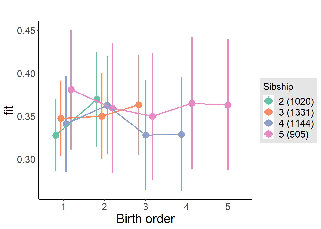
Model Comparison
###### Model 1 - Model 2
anova(m1_covariates_only, m2_birthorder_linear, m3_birthorder_nonlinear, m4_interaction)## refitting model(s) with ML (instead of REML)| Df | AIC | BIC | logLik | deviance | Chisq | Chi Df | Pr(>Chisq) |
|---|---|---|---|---|---|---|---|
| 10 | 3104 | 3168 | -1542 | 3084 | NA | NA | NA |
| 11 | 3106 | 3176 | -1542 | 3084 | 0.002569 | 1 | 0.9596 |
| 14 | 3110 | 3199 | -1541 | 3082 | 2.191 | 3 | 0.5338 |
| 20 | 3117 | 3245 | -1538 | 3077 | 4.856 | 6 | 0.5625 |
Parental full sibling order
outcome_parental_m1 <- update(m2_birthorder_linear, data = birthorder %>%
mutate(sibling_count = sibling_count_genes_factor,
birth_order_nonlinear = birthorder_genes_factor,
birth_order = birthorder_genes,
count_birth_order = count_birthorder_genes
) %>%
filter(sibling_count != "1"))
compare_models_markdown(outcome_parental_m1)Basic Model
Model Summary
m1_covariates_only <- update(m2_birthorder_linear, formula = . ~ . - birth_order)
tidy(m1_covariates_only, conf.int = T, conf.level = 0.995)| effect | group | term | estimate | std.error | statistic | df | p.value | conf.low | conf.high |
|---|---|---|---|---|---|---|---|---|---|
| fixed | NA | (Intercept) | -1.707 | 0.1866 | -9.144 | 4703 | 8.738e-20 | -2.231 | -1.183 |
| fixed | NA | poly(age, 3, raw = TRUE)1 | 0.1645 | 0.02183 | 7.536 | 4709 | 5.78e-14 | 0.1032 | 0.2258 |
| fixed | NA | poly(age, 3, raw = TRUE)2 | -0.004886 | 0.0008064 | -6.059 | 4714 | 0.000000001476 | -0.00715 | -0.002622 |
| fixed | NA | poly(age, 3, raw = TRUE)3 | 0.00004705 | 0.000009477 | 4.965 | 4716 | 0.0000007105 | 0.00002045 | 0.00007365 |
| fixed | NA | male | 0.5556 | 0.009933 | 55.94 | 4606 | 0 | 0.5278 | 0.5835 |
| fixed | NA | sibling_count3 | 0.003996 | 0.01357 | 0.2945 | 3399 | 0.7684 | -0.03409 | 0.04209 |
| fixed | NA | sibling_count4 | -0.0005728 | 0.01478 | -0.03875 | 2998 | 0.9691 | -0.04207 | 0.04092 |
| fixed | NA | sibling_count5 | 0.01582 | 0.01756 | 0.9008 | 2595 | 0.3678 | -0.03347 | 0.0651 |
| ran_pars | mother_pidlink | sd__(Intercept) | 0.1371 | NA | NA | NA | NA | NA | NA |
| ran_pars | Residual | sd__Observation | 0.3162 | NA | NA | NA | NA | NA | NA |
Coefficient Plot
plot(allEffects(m1_covariates_only, confidence.level = 0.995))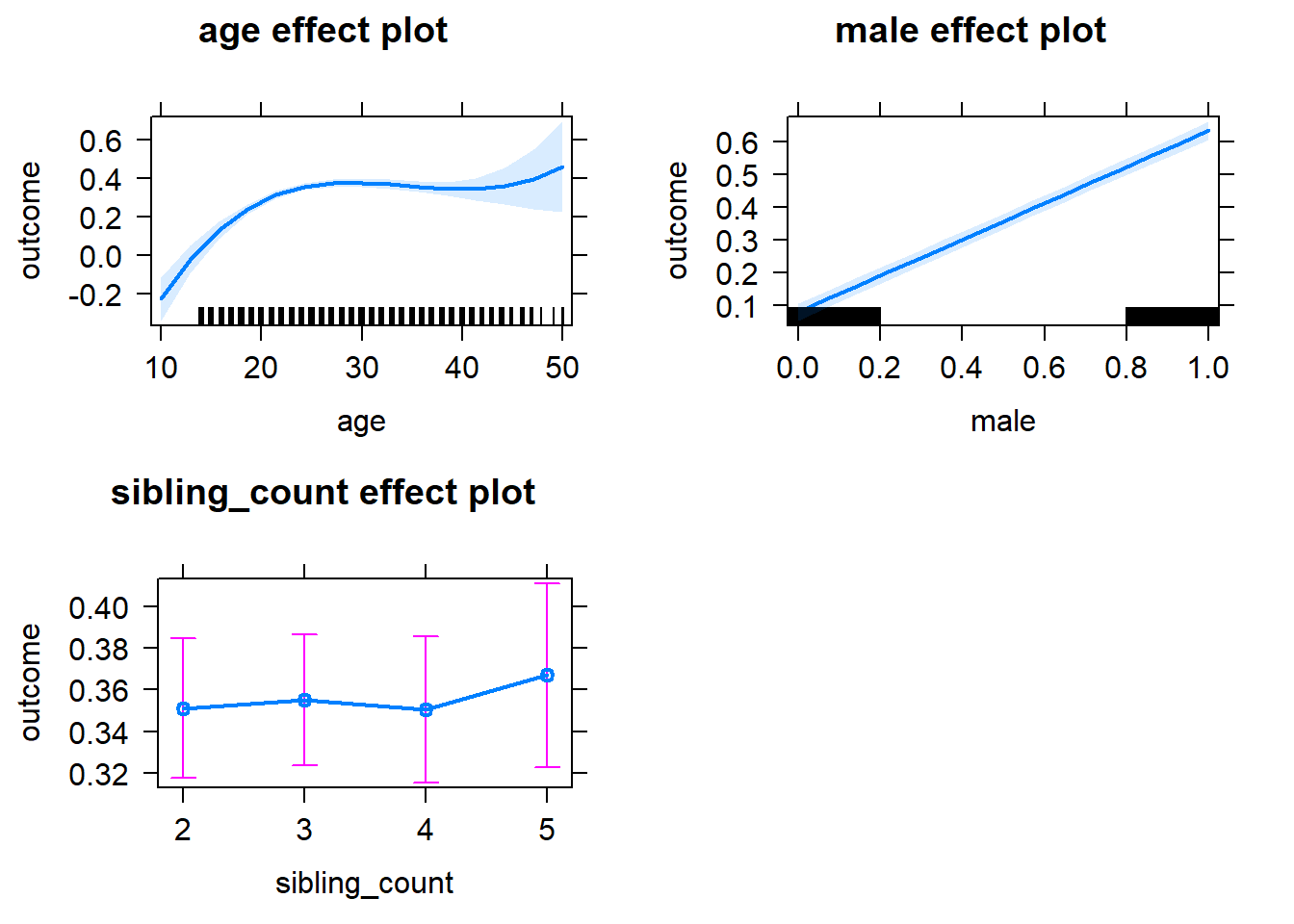
Add Birth Order Linear
Model Summary
tidy(m2_birthorder_linear, conf.int = T, conf.level = 0.995)| effect | group | term | estimate | std.error | statistic | df | p.value | conf.low | conf.high |
|---|---|---|---|---|---|---|---|---|---|
| fixed | NA | (Intercept) | -1.714 | 0.1869 | -9.17 | 4703 | 6.911e-20 | -2.238 | -1.189 |
| fixed | NA | birth_order | 0.003948 | 0.005265 | 0.7498 | 4293 | 0.4534 | -0.01083 | 0.01873 |
| fixed | NA | poly(age, 3, raw = TRUE)1 | 0.1647 | 0.02183 | 7.546 | 4708 | 5.344e-14 | 0.1035 | 0.226 |
| fixed | NA | poly(age, 3, raw = TRUE)2 | -0.004899 | 0.0008066 | -6.074 | 4713 | 0.000000001349 | -0.007163 | -0.002635 |
| fixed | NA | poly(age, 3, raw = TRUE)3 | 0.00004728 | 0.000009482 | 4.987 | 4715 | 0.0000006362 | 0.00002067 | 0.0000739 |
| fixed | NA | male | 0.5556 | 0.009934 | 55.93 | 4605 | 0 | 0.5277 | 0.5834 |
| fixed | NA | sibling_count3 | 0.002145 | 0.01379 | 0.1556 | 3458 | 0.8764 | -0.03657 | 0.04086 |
| fixed | NA | sibling_count4 | -0.004748 | 0.0158 | -0.3006 | 3240 | 0.7638 | -0.04909 | 0.03959 |
| fixed | NA | sibling_count5 | 0.009144 | 0.01968 | 0.4646 | 3076 | 0.6422 | -0.0461 | 0.06439 |
| ran_pars | mother_pidlink | sd__(Intercept) | 0.137 | NA | NA | NA | NA | NA | NA |
| ran_pars | Residual | sd__Observation | 0.3162 | NA | NA | NA | NA | NA | NA |
Coefficient Plot
plot_birthorder2(m2_birthorder_linear, separate = FALSE)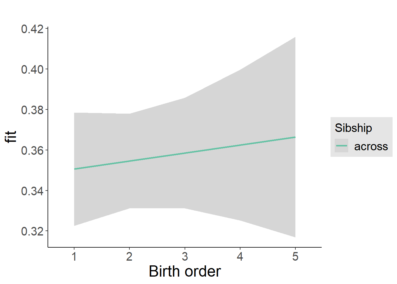
Add Birth Order Factor
Model Summary
m3_birthorder_nonlinear = update(m1_covariates_only, formula = . ~ . + birth_order_nonlinear)
tidy(m3_birthorder_nonlinear, conf.int = T, conf.level = 0.995)| effect | group | term | estimate | std.error | statistic | df | p.value | conf.low | conf.high |
|---|---|---|---|---|---|---|---|---|---|
| fixed | NA | (Intercept) | -1.729 | 0.1872 | -9.238 | 4706 | 3.707e-20 | -2.254 | -1.204 |
| fixed | NA | poly(age, 3, raw = TRUE)1 | 0.1663 | 0.02186 | 7.607 | 4709 | 3.359e-14 | 0.105 | 0.2277 |
| fixed | NA | poly(age, 3, raw = TRUE)2 | -0.004954 | 0.0008077 | -6.134 | 4712 | 0.0000000009295 | -0.007222 | -0.002687 |
| fixed | NA | poly(age, 3, raw = TRUE)3 | 0.00004786 | 0.000009493 | 5.042 | 4713 | 0.0000004782 | 0.00002122 | 0.00007451 |
| fixed | NA | male | 0.5558 | 0.009936 | 55.94 | 4601 | 0 | 0.5279 | 0.5837 |
| fixed | NA | sibling_count3 | 0.001336 | 0.014 | 0.09543 | 3588 | 0.924 | -0.03797 | 0.04065 |
| fixed | NA | sibling_count4 | -0.002221 | 0.01602 | -0.1386 | 3350 | 0.8897 | -0.04719 | 0.04275 |
| fixed | NA | sibling_count5 | 0.01349 | 0.02007 | 0.6723 | 3197 | 0.5015 | -0.04284 | 0.06982 |
| fixed | NA | birth_order_nonlinear2 | 0.01982 | 0.01163 | 1.705 | 3691 | 0.08829 | -0.01281 | 0.05246 |
| fixed | NA | birth_order_nonlinear3 | 0.01355 | 0.0149 | 0.9094 | 3917 | 0.3632 | -0.02828 | 0.05539 |
| fixed | NA | birth_order_nonlinear4 | -0.0005506 | 0.02064 | -0.02667 | 4109 | 0.9787 | -0.05849 | 0.05739 |
| fixed | NA | birth_order_nonlinear5 | 0.01623 | 0.03375 | 0.4809 | 3974 | 0.6306 | -0.07851 | 0.111 |
| ran_pars | mother_pidlink | sd__(Intercept) | 0.1367 | NA | NA | NA | NA | NA | NA |
| ran_pars | Residual | sd__Observation | 0.3163 | NA | NA | NA | NA | NA | NA |
Coefficient Plot
plot_birthorder(m3_birthorder_nonlinear, separate = FALSE)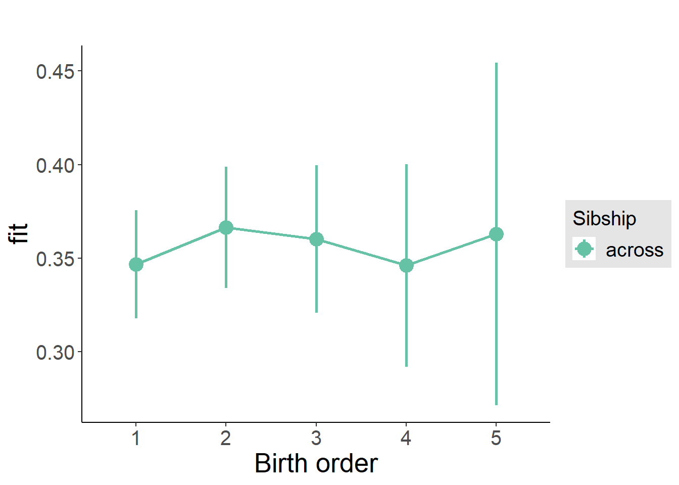
Add Interaction
Model Summary
m4_interaction = update(m3_birthorder_nonlinear, formula = . ~ . - birth_order_nonlinear - sibling_count + count_birth_order)
tidy(m4_interaction, conf.int = T, conf.level = 0.995)| effect | group | term | estimate | std.error | statistic | df | p.value | conf.low | conf.high |
|---|---|---|---|---|---|---|---|---|---|
| fixed | NA | (Intercept) | -1.729 | 0.1873 | -9.234 | 4700 | 3.86e-20 | -2.255 | -1.204 |
| fixed | NA | poly(age, 3, raw = TRUE)1 | 0.1656 | 0.02188 | 7.572 | 4703 | 4.412e-14 | 0.1042 | 0.2271 |
| fixed | NA | poly(age, 3, raw = TRUE)2 | -0.00493 | 0.0008083 | -6.099 | 4705 | 0.000000001149 | -0.007199 | -0.002661 |
| fixed | NA | poly(age, 3, raw = TRUE)3 | 0.00004759 | 0.0000095 | 5.01 | 4707 | 0.0000005656 | 0.00002092 | 0.00007426 |
| fixed | NA | male | 0.5556 | 0.009943 | 55.89 | 4595 | 0 | 0.5277 | 0.5836 |
| fixed | NA | count_birth_order2/2 | 0.03848 | 0.01947 | 1.977 | 3849 | 0.04815 | -0.01616 | 0.09312 |
| fixed | NA | count_birth_order1/3 | 0.01826 | 0.01779 | 1.026 | 4687 | 0.3048 | -0.03167 | 0.06819 |
| fixed | NA | count_birth_order2/3 | 0.01654 | 0.01956 | 0.8459 | 4707 | 0.3977 | -0.03836 | 0.07145 |
| fixed | NA | count_birth_order3/3 | 0.01559 | 0.02146 | 0.7263 | 4700 | 0.4677 | -0.04465 | 0.07582 |
| fixed | NA | count_birth_order1/4 | -0.006886 | 0.02208 | -0.3119 | 4705 | 0.7551 | -0.06887 | 0.05509 |
| fixed | NA | count_birth_order2/4 | 0.0283 | 0.02271 | 1.246 | 4704 | 0.2128 | -0.03545 | 0.09204 |
| fixed | NA | count_birth_order3/4 | 0.02324 | 0.02377 | 0.9776 | 4683 | 0.3283 | -0.04349 | 0.08996 |
| fixed | NA | count_birth_order4/4 | 0.007944 | 0.02508 | 0.3167 | 4673 | 0.7515 | -0.06247 | 0.07836 |
| fixed | NA | count_birth_order1/5 | 0.03237 | 0.02995 | 1.081 | 4705 | 0.2799 | -0.05171 | 0.1164 |
| fixed | NA | count_birth_order2/5 | 0.02752 | 0.03313 | 0.8307 | 4652 | 0.4062 | -0.06547 | 0.1205 |
| fixed | NA | count_birth_order3/5 | 0.03652 | 0.03116 | 1.172 | 4657 | 0.2413 | -0.05096 | 0.124 |
| fixed | NA | count_birth_order4/5 | 0.01262 | 0.03054 | 0.4133 | 4665 | 0.6794 | -0.07311 | 0.09836 |
| fixed | NA | count_birth_order5/5 | 0.03596 | 0.03227 | 1.114 | 4641 | 0.2653 | -0.05464 | 0.1266 |
| ran_pars | mother_pidlink | sd__(Intercept) | 0.1365 | NA | NA | NA | NA | NA | NA |
| ran_pars | Residual | sd__Observation | 0.3165 | NA | NA | NA | NA | NA | NA |
Coefficient Plot
plot_birthorder(m4_interaction)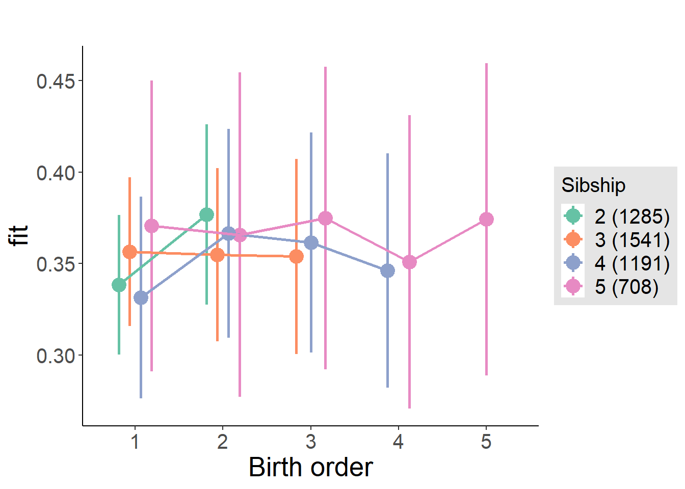
Model Comparison
###### Model 1 - Model 2
anova(m1_covariates_only, m2_birthorder_linear, m3_birthorder_nonlinear, m4_interaction)## refitting model(s) with ML (instead of REML)| Df | AIC | BIC | logLik | deviance | Chisq | Chi Df | Pr(>Chisq) |
|---|---|---|---|---|---|---|---|
| 10 | 3306 | 3371 | -1643 | 3286 | NA | NA | NA |
| 11 | 3308 | 3379 | -1643 | 3286 | 0.5636 | 1 | 0.4528 |
| 14 | 3311 | 3401 | -1641 | 3283 | 2.883 | 3 | 0.41 |
| 20 | 3319 | 3449 | -1640 | 3279 | 3.289 | 6 | 0.7718 |
Compare birth order specifications
library(coefplot)
multiplot(outcome_naive_m1, outcome_preg_m1, outcome_uterus_m1, outcome_parental_m1, dodgeHeight = 0.6,
intercept = FALSE)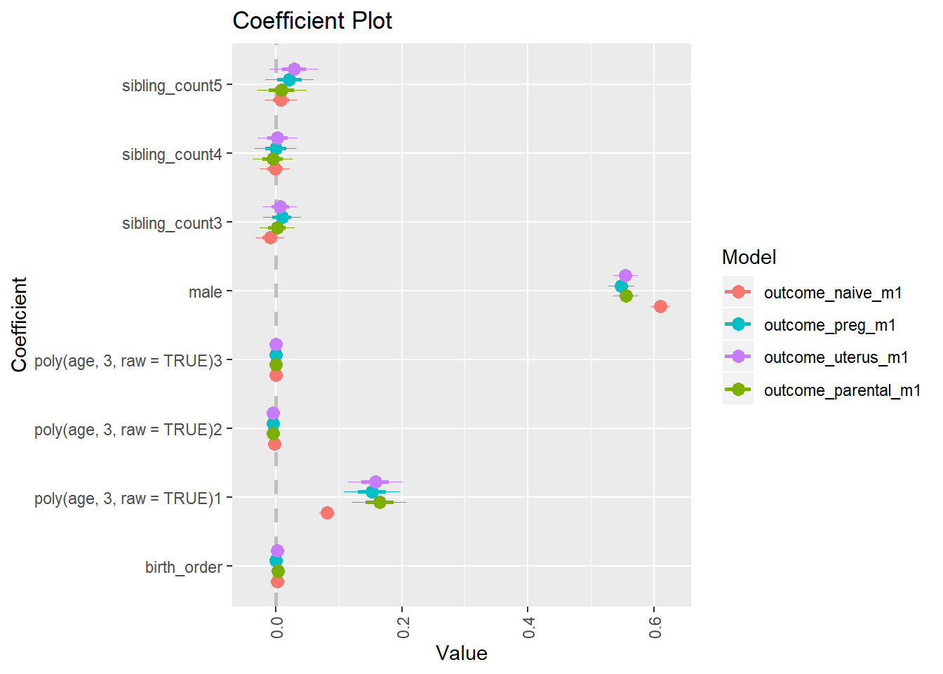
still_smoking
birthorder <- birthorder %>% mutate(outcome = still_smoking)
model = lmer(outcome ~ birth_order + poly(age, 3, raw = TRUE) + male + sibling_count + (1 | mother_pidlink),
data = birthorder)
compare_birthorder_specs(model)Naive birth order
outcome_naive_m1 <- update(m2_birthorder_linear, data = birthorder %>%
mutate(sibling_count = sibling_count_naive_factor,
birth_order_nonlinear = birthorder_naive_factor,
birth_order = birthorder_naive,
count_birth_order = count_birthorder_naive) %>%
filter(sibling_count != "1"))
compare_models_markdown(outcome_naive_m1)Basic Model
Model Summary
m1_covariates_only <- update(m2_birthorder_linear, formula = . ~ . - birth_order)
tidy(m1_covariates_only, conf.int = T, conf.level = 0.995)| effect | group | term | estimate | std.error | statistic | df | p.value | conf.low | conf.high |
|---|---|---|---|---|---|---|---|---|---|
| fixed | NA | (Intercept) | 0.3968 | 0.1066 | 3.722 | 2209 | 0.0002026 | 0.09753 | 0.696 |
| fixed | NA | poly(age, 3, raw = TRUE)1 | 0.023 | 0.008962 | 2.567 | 2051 | 0.01033 | -0.002151 | 0.04816 |
| fixed | NA | poly(age, 3, raw = TRUE)2 | -0.0006366 | 0.0002435 | -2.614 | 1898 | 0.009019 | -0.00132 | 0.00004701 |
| fixed | NA | poly(age, 3, raw = TRUE)3 | 0.000005083 | 0.000002062 | 2.465 | 1720 | 0.0138 | -0.0000007052 | 0.00001087 |
| fixed | NA | male | 0.2759 | 0.03476 | 7.936 | 2330 | 3.219e-15 | 0.1783 | 0.3734 |
| fixed | NA | sibling_count3 | 0.01577 | 0.01672 | 0.9432 | 1903 | 0.3457 | -0.03116 | 0.0627 |
| fixed | NA | sibling_count4 | 0.003126 | 0.01683 | 0.1857 | 1777 | 0.8527 | -0.04413 | 0.05038 |
| fixed | NA | sibling_count5 | 0.009951 | 0.01747 | 0.5695 | 1659 | 0.5691 | -0.03909 | 0.059 |
| ran_pars | mother_pidlink | sd__(Intercept) | 0.07966 | NA | NA | NA | NA | NA | NA |
| ran_pars | Residual | sd__Observation | 0.2708 | NA | NA | NA | NA | NA | NA |
Coefficient Plot
plot(allEffects(m1_covariates_only, confidence.level = 0.995))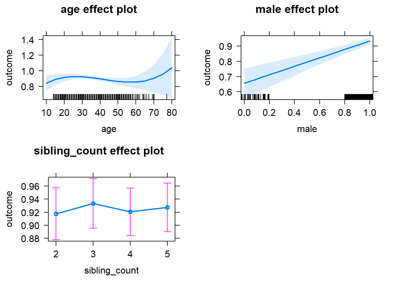
Add Birth Order Linear
Model Summary
tidy(m2_birthorder_linear, conf.int = T, conf.level = 0.995)| effect | group | term | estimate | std.error | statistic | df | p.value | conf.low | conf.high |
|---|---|---|---|---|---|---|---|---|---|
| fixed | NA | (Intercept) | 0.3953 | 0.1066 | 3.708 | 2208 | 0.0002144 | 0.09602 | 0.6946 |
| fixed | NA | birth_order | 0.004797 | 0.005766 | 0.832 | 2140 | 0.4055 | -0.01139 | 0.02098 |
| fixed | NA | poly(age, 3, raw = TRUE)1 | 0.0225 | 0.008983 | 2.505 | 2052 | 0.01234 | -0.002717 | 0.04771 |
| fixed | NA | poly(age, 3, raw = TRUE)2 | -0.0006234 | 0.0002441 | -2.554 | 1897 | 0.01072 | -0.001309 | 0.00006168 |
| fixed | NA | poly(age, 3, raw = TRUE)3 | 0.000004993 | 0.000002065 | 2.418 | 1719 | 0.01573 | -0.0000008042 | 0.00001079 |
| fixed | NA | male | 0.2756 | 0.03477 | 7.926 | 2329 | 3.464e-15 | 0.178 | 0.3732 |
| fixed | NA | sibling_count3 | 0.0138 | 0.01689 | 0.8172 | 1940 | 0.4139 | -0.0336 | 0.0612 |
| fixed | NA | sibling_count4 | -0.0007215 | 0.01746 | -0.04133 | 1913 | 0.967 | -0.04973 | 0.04829 |
| fixed | NA | sibling_count5 | 0.003878 | 0.01894 | 0.2048 | 1943 | 0.8378 | -0.04928 | 0.05704 |
| ran_pars | mother_pidlink | sd__(Intercept) | 0.07975 | NA | NA | NA | NA | NA | NA |
| ran_pars | Residual | sd__Observation | 0.2708 | NA | NA | NA | NA | NA | NA |
Coefficient Plot
plot_birthorder2(m2_birthorder_linear, separate = FALSE)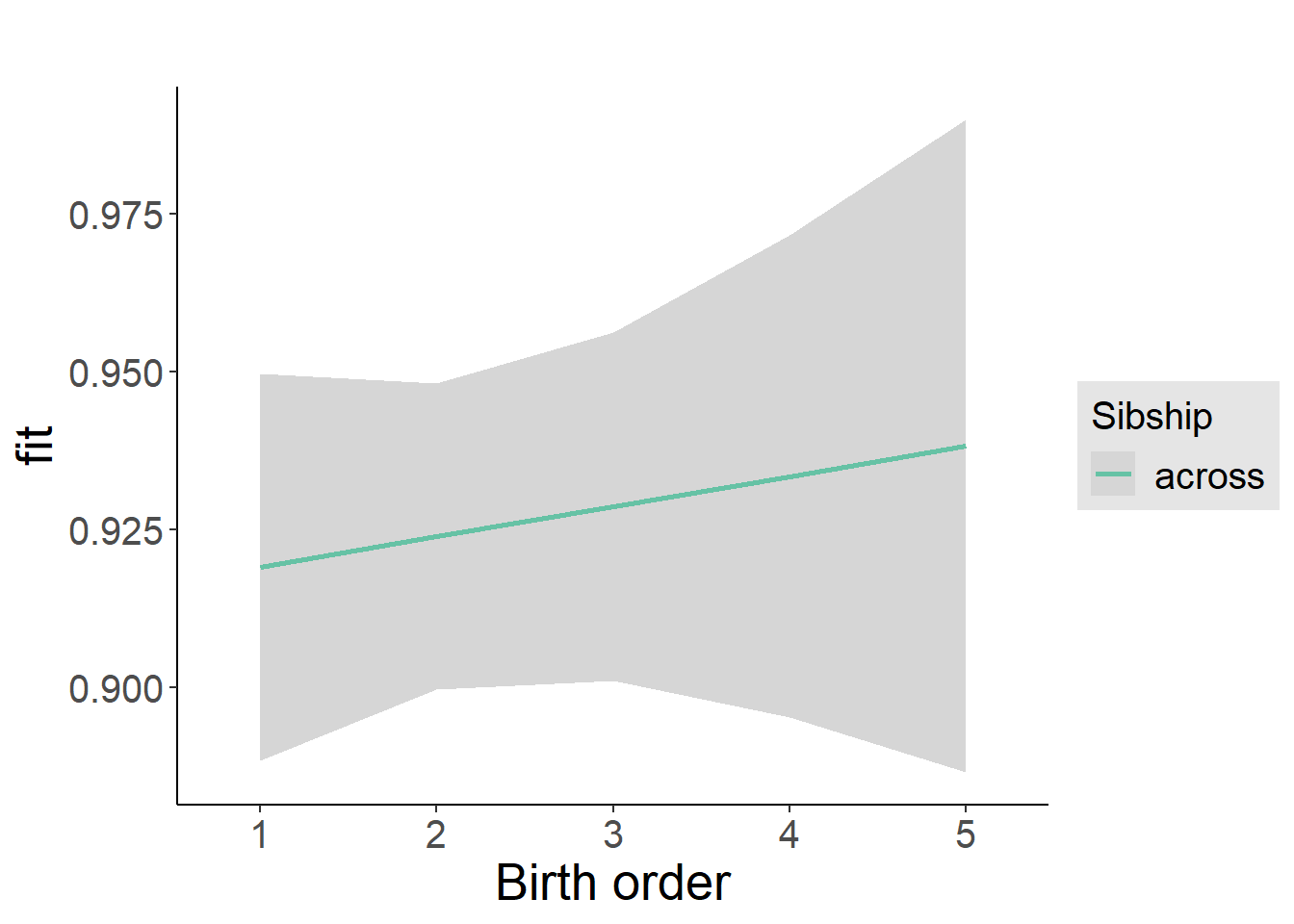
Add Birth Order Factor
Model Summary
m3_birthorder_nonlinear = update(m1_covariates_only, formula = . ~ . + birth_order_nonlinear)
tidy(m3_birthorder_nonlinear, conf.int = T, conf.level = 0.995)| effect | group | term | estimate | std.error | statistic | df | p.value | conf.low | conf.high |
|---|---|---|---|---|---|---|---|---|---|
| fixed | NA | (Intercept) | 0.4011 | 0.1066 | 3.761 | 2209 | 0.0001734 | 0.1018 | 0.7003 |
| fixed | NA | poly(age, 3, raw = TRUE)1 | 0.02251 | 0.008979 | 2.508 | 2051 | 0.01223 | -0.002689 | 0.04772 |
| fixed | NA | poly(age, 3, raw = TRUE)2 | -0.0006194 | 0.0002439 | -2.539 | 1895 | 0.01119 | -0.001304 | 0.0000653 |
| fixed | NA | poly(age, 3, raw = TRUE)3 | 0.000004923 | 0.000002064 | 2.386 | 1716 | 0.01716 | -0.0000008698 | 0.00001072 |
| fixed | NA | male | 0.2756 | 0.03474 | 7.935 | 2326 | 3.248e-15 | 0.1781 | 0.3732 |
| fixed | NA | sibling_count3 | 0.02249 | 0.01724 | 1.304 | 2010 | 0.1924 | -0.02592 | 0.07089 |
| fixed | NA | sibling_count4 | 0.003533 | 0.01779 | 0.1986 | 1966 | 0.8426 | -0.04641 | 0.05348 |
| fixed | NA | sibling_count5 | 0.0008832 | 0.01921 | 0.04598 | 1989 | 0.9633 | -0.05304 | 0.05481 |
| fixed | NA | birth_order_nonlinear2 | -0.002417 | 0.01404 | -0.1722 | 2117 | 0.8633 | -0.04181 | 0.03698 |
| fixed | NA | birth_order_nonlinear3 | -0.02579 | 0.01777 | -1.451 | 2110 | 0.1468 | -0.07566 | 0.02409 |
| fixed | NA | birth_order_nonlinear4 | 0.02512 | 0.0223 | 1.127 | 2119 | 0.26 | -0.03747 | 0.08772 |
| fixed | NA | birth_order_nonlinear5 | 0.05765 | 0.03472 | 1.661 | 2122 | 0.09695 | -0.03981 | 0.1551 |
| ran_pars | mother_pidlink | sd__(Intercept) | 0.07991 | NA | NA | NA | NA | NA | NA |
| ran_pars | Residual | sd__Observation | 0.2705 | NA | NA | NA | NA | NA | NA |
Coefficient Plot
plot_birthorder(m3_birthorder_nonlinear, separate = FALSE)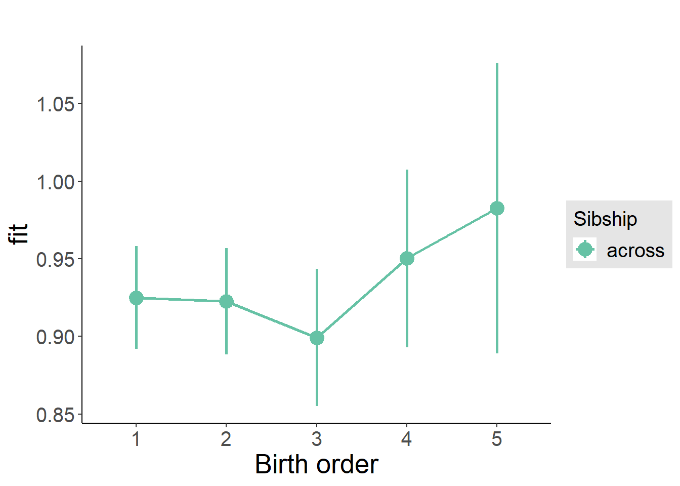
Add Interaction
Model Summary
m4_interaction = update(m3_birthorder_nonlinear, formula = . ~ . - birth_order_nonlinear - sibling_count + count_birth_order)
tidy(m4_interaction, conf.int = T, conf.level = 0.995)| effect | group | term | estimate | std.error | statistic | df | p.value | conf.low | conf.high |
|---|---|---|---|---|---|---|---|---|---|
| fixed | NA | (Intercept) | 0.3958 | 0.1069 | 3.704 | 2206 | 0.0002177 | 0.09582 | 0.6958 |
| fixed | NA | poly(age, 3, raw = TRUE)1 | 0.02236 | 0.008988 | 2.488 | 2046 | 0.01293 | -0.00287 | 0.04759 |
| fixed | NA | poly(age, 3, raw = TRUE)2 | -0.0006152 | 0.0002441 | -2.521 | 1889 | 0.01179 | -0.0013 | 0.00006988 |
| fixed | NA | poly(age, 3, raw = TRUE)3 | 0.000004896 | 0.000002064 | 2.372 | 1708 | 0.01781 | -0.0000008984 | 0.00001069 |
| fixed | NA | male | 0.275 | 0.03475 | 7.914 | 2320 | 3.828e-15 | 0.1775 | 0.3726 |
| fixed | NA | count_birth_order2/2 | 0.01497 | 0.02387 | 0.6268 | 2085 | 0.5308 | -0.05205 | 0.08198 |
| fixed | NA | count_birth_order1/3 | 0.02417 | 0.02377 | 1.017 | 2321 | 0.3093 | -0.04256 | 0.0909 |
| fixed | NA | count_birth_order2/3 | 0.03211 | 0.02528 | 1.27 | 2321 | 0.2042 | -0.03887 | 0.1031 |
| fixed | NA | count_birth_order3/3 | 0.006457 | 0.02736 | 0.236 | 2321 | 0.8134 | -0.07033 | 0.08325 |
| fixed | NA | count_birth_order1/4 | 0.001714 | 0.0253 | 0.06774 | 2321 | 0.946 | -0.06931 | 0.07274 |
| fixed | NA | count_birth_order2/4 | 0.007243 | 0.02719 | 0.2664 | 2319 | 0.79 | -0.06908 | 0.08357 |
| fixed | NA | count_birth_order3/4 | -0.001215 | 0.02931 | -0.04144 | 2320 | 0.9669 | -0.0835 | 0.08107 |
| fixed | NA | count_birth_order4/4 | 0.03801 | 0.0301 | 1.263 | 2321 | 0.2068 | -0.04649 | 0.1225 |
| fixed | NA | count_birth_order1/5 | 0.04659 | 0.02818 | 1.653 | 2319 | 0.09839 | -0.03251 | 0.1257 |
| fixed | NA | count_birth_order2/5 | -0.02261 | 0.03104 | -0.7285 | 2314 | 0.4664 | -0.1097 | 0.06452 |
| fixed | NA | count_birth_order3/5 | -0.03955 | 0.03235 | -1.223 | 2317 | 0.2215 | -0.1303 | 0.05124 |
| fixed | NA | count_birth_order4/5 | 0.03088 | 0.0317 | 0.9744 | 2316 | 0.33 | -0.05809 | 0.1199 |
| fixed | NA | count_birth_order5/5 | 0.06597 | 0.03501 | 1.884 | 2313 | 0.05968 | -0.03232 | 0.1643 |
| ran_pars | mother_pidlink | sd__(Intercept) | 0.07912 | NA | NA | NA | NA | NA | NA |
| ran_pars | Residual | sd__Observation | 0.2708 | NA | NA | NA | NA | NA | NA |
Coefficient Plot
plot_birthorder(m4_interaction)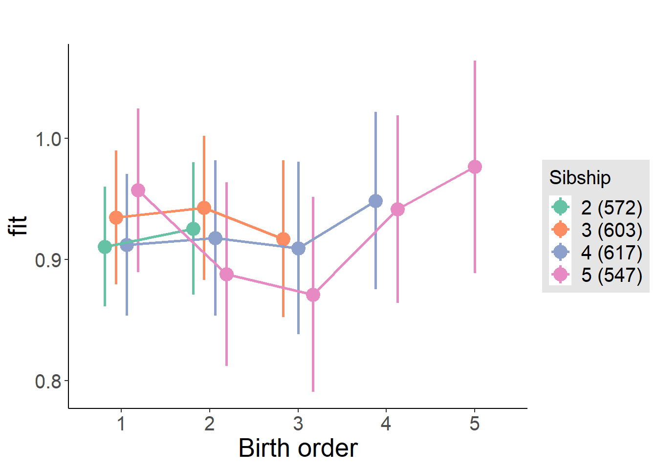
Model Comparison
###### Model 1 - Model 2
anova(m1_covariates_only, m2_birthorder_linear, m3_birthorder_nonlinear, m4_interaction)## refitting model(s) with ML (instead of REML)| Df | AIC | BIC | logLik | deviance | Chisq | Chi Df | Pr(>Chisq) |
|---|---|---|---|---|---|---|---|
| 10 | 729.8 | 787.4 | -354.9 | 709.8 | NA | NA | NA |
| 11 | 731.1 | 794.5 | -354.6 | 709.1 | 0.6939 | 1 | 0.4049 |
| 14 | 730.1 | 810.7 | -351 | 702.1 | 7.08 | 3 | 0.06939 |
| 20 | 736.3 | 851.4 | -348.1 | 696.3 | 5.769 | 6 | 0.4495 |
Maternal birth order
outcome_uterus_m1 <- update(m2_birthorder_linear, data = birthorder %>%
mutate(sibling_count = sibling_count_uterus_alive_factor,
birth_order_nonlinear = birthorder_uterus_alive_factor,
birth_order = birthorder_uterus_alive,
count_birth_order = count_birthorder_uterus_alive) %>%
filter(sibling_count != "1"))
compare_models_markdown(outcome_uterus_m1)Basic Model
Model Summary
m1_covariates_only <- update(m2_birthorder_linear, formula = . ~ . - birth_order)
tidy(m1_covariates_only, conf.int = T, conf.level = 0.995)| effect | group | term | estimate | std.error | statistic | df | p.value | conf.low | conf.high |
|---|---|---|---|---|---|---|---|---|---|
| fixed | NA | (Intercept) | -0.3133 | 0.3052 | -1.026 | 1324 | 0.3049 | -1.17 | 0.5436 |
| fixed | NA | poly(age, 3, raw = TRUE)1 | 0.09584 | 0.03384 | 2.832 | 1322 | 0.004694 | 0.00085 | 0.1908 |
| fixed | NA | poly(age, 3, raw = TRUE)2 | -0.003267 | 0.001213 | -2.694 | 1320 | 0.007153 | -0.006672 | 0.0001373 |
| fixed | NA | poly(age, 3, raw = TRUE)3 | 0.00003403 | 0.0000139 | 2.447 | 1319 | 0.01453 | -0.000005003 | 0.00007306 |
| fixed | NA | male | 0.3579 | 0.05252 | 6.816 | 1328 | 0.00000000001417 | 0.2105 | 0.5054 |
| fixed | NA | sibling_count3 | 0.01207 | 0.02094 | 0.5765 | 1141 | 0.5644 | -0.04671 | 0.07085 |
| fixed | NA | sibling_count4 | 0.03844 | 0.02207 | 1.741 | 1083 | 0.08189 | -0.02352 | 0.1004 |
| fixed | NA | sibling_count5 | 0.03008 | 0.02412 | 1.247 | 979.3 | 0.2127 | -0.03763 | 0.09779 |
| ran_pars | mother_pidlink | sd__(Intercept) | 0.04403 | NA | NA | NA | NA | NA | NA |
| ran_pars | Residual | sd__Observation | 0.2749 | NA | NA | NA | NA | NA | NA |
Coefficient Plot
plot(allEffects(m1_covariates_only, confidence.level = 0.995))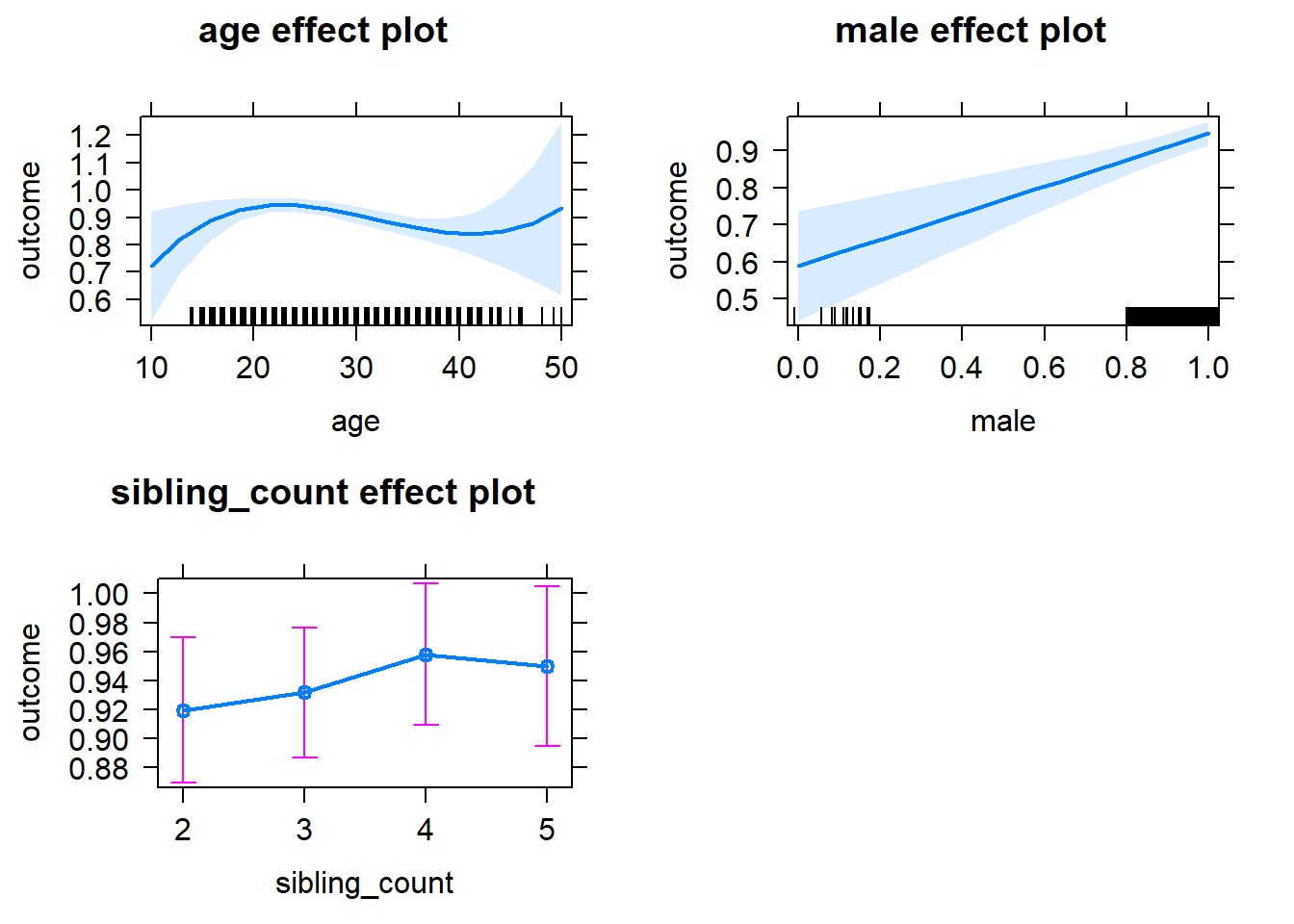
Add Birth Order Linear
Model Summary
tidy(m2_birthorder_linear, conf.int = T, conf.level = 0.995)| effect | group | term | estimate | std.error | statistic | df | p.value | conf.low | conf.high |
|---|---|---|---|---|---|---|---|---|---|
| fixed | NA | (Intercept) | -0.3059 | 0.3056 | -1.001 | 1323 | 0.317 | -1.164 | 0.5519 |
| fixed | NA | birth_order | -0.005042 | 0.007896 | -0.6385 | 1316 | 0.5232 | -0.02721 | 0.01712 |
| fixed | NA | poly(age, 3, raw = TRUE)1 | 0.09569 | 0.03385 | 2.827 | 1321 | 0.00477 | 0.0006745 | 0.1907 |
| fixed | NA | poly(age, 3, raw = TRUE)2 | -0.003258 | 0.001213 | -2.685 | 1319 | 0.00735 | -0.006663 | 0.0001484 |
| fixed | NA | poly(age, 3, raw = TRUE)3 | 0.00003383 | 0.00001391 | 2.431 | 1318 | 0.01517 | -0.000005225 | 0.00007288 |
| fixed | NA | male | 0.3584 | 0.05253 | 6.822 | 1327 | 0.00000000001363 | 0.2109 | 0.5058 |
| fixed | NA | sibling_count3 | 0.01421 | 0.02122 | 0.6698 | 1152 | 0.5031 | -0.04535 | 0.07377 |
| fixed | NA | sibling_count4 | 0.04369 | 0.02356 | 1.854 | 1112 | 0.06397 | -0.02245 | 0.1098 |
| fixed | NA | sibling_count5 | 0.03869 | 0.0276 | 1.402 | 1093 | 0.1612 | -0.03878 | 0.1162 |
| ran_pars | mother_pidlink | sd__(Intercept) | 0.04661 | NA | NA | NA | NA | NA | NA |
| ran_pars | Residual | sd__Observation | 0.2745 | NA | NA | NA | NA | NA | NA |
Coefficient Plot
plot_birthorder2(m2_birthorder_linear, separate = FALSE)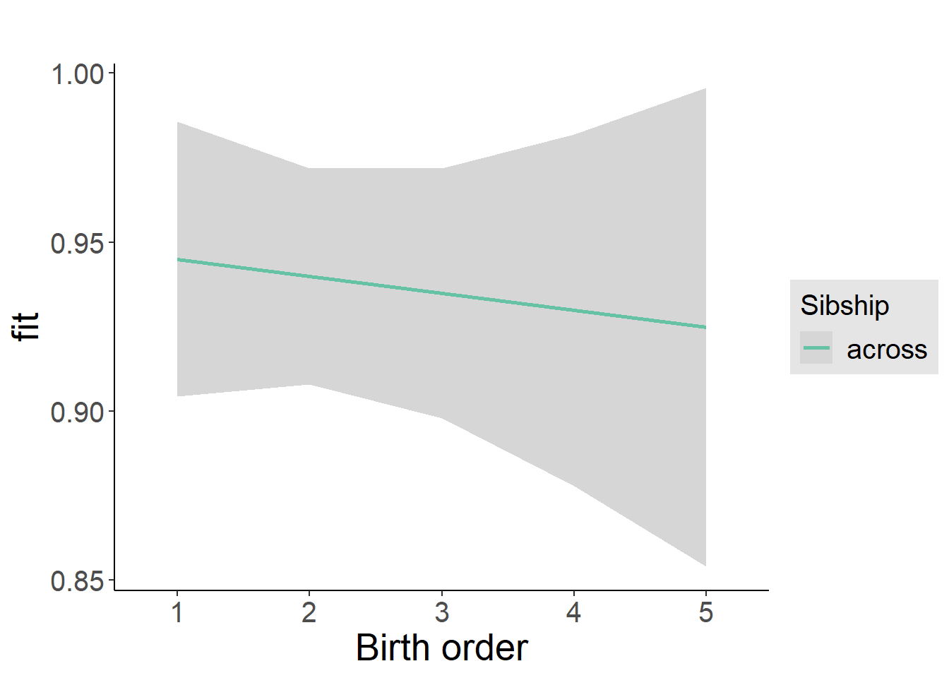
Add Birth Order Factor
Model Summary
m3_birthorder_nonlinear = update(m1_covariates_only, formula = . ~ . + birth_order_nonlinear)
tidy(m3_birthorder_nonlinear, conf.int = T, conf.level = 0.995)| effect | group | term | estimate | std.error | statistic | df | p.value | conf.low | conf.high |
|---|---|---|---|---|---|---|---|---|---|
| fixed | NA | (Intercept) | -0.3127 | 0.3056 | -1.023 | 1320 | 0.3065 | -1.171 | 0.5452 |
| fixed | NA | poly(age, 3, raw = TRUE)1 | 0.09628 | 0.03389 | 2.841 | 1318 | 0.004565 | 0.001156 | 0.1914 |
| fixed | NA | poly(age, 3, raw = TRUE)2 | -0.00328 | 0.001215 | -2.7 | 1316 | 0.007021 | -0.00669 | 0.0001299 |
| fixed | NA | poly(age, 3, raw = TRUE)3 | 0.00003412 | 0.00001393 | 2.449 | 1315 | 0.01444 | -0.000004983 | 0.00007322 |
| fixed | NA | male | 0.3588 | 0.05258 | 6.823 | 1325 | 0.00000000001352 | 0.2112 | 0.5064 |
| fixed | NA | sibling_count3 | 0.01497 | 0.02161 | 0.6924 | 1180 | 0.4888 | -0.0457 | 0.07563 |
| fixed | NA | sibling_count4 | 0.04146 | 0.02399 | 1.728 | 1130 | 0.08427 | -0.02589 | 0.1088 |
| fixed | NA | sibling_count5 | 0.03627 | 0.02815 | 1.289 | 1101 | 0.1978 | -0.04274 | 0.1153 |
| fixed | NA | birth_order_nonlinear2 | -0.01501 | 0.01863 | -0.8057 | 1213 | 0.4206 | -0.0673 | 0.03728 |
| fixed | NA | birth_order_nonlinear3 | -0.01689 | 0.02281 | -0.7401 | 1232 | 0.4594 | -0.08092 | 0.04715 |
| fixed | NA | birth_order_nonlinear4 | -0.002029 | 0.03051 | -0.06651 | 1303 | 0.947 | -0.08766 | 0.0836 |
| fixed | NA | birth_order_nonlinear5 | -0.02822 | 0.04732 | -0.5964 | 1290 | 0.551 | -0.161 | 0.1046 |
| ran_pars | mother_pidlink | sd__(Intercept) | 0.04722 | NA | NA | NA | NA | NA | NA |
| ran_pars | Residual | sd__Observation | 0.2747 | NA | NA | NA | NA | NA | NA |
Coefficient Plot
plot_birthorder(m3_birthorder_nonlinear, separate = FALSE)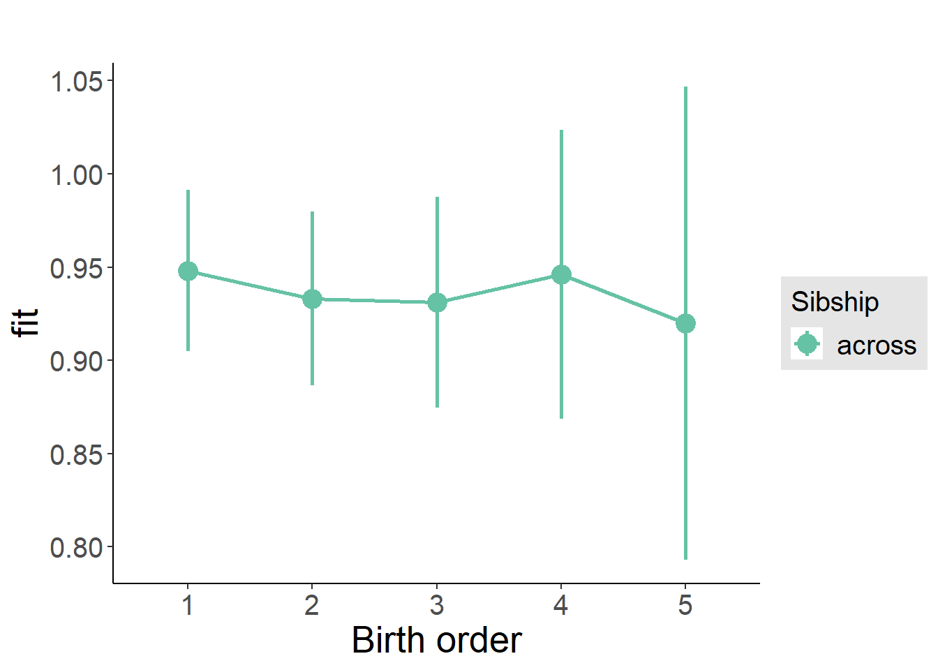
Add Interaction
Model Summary
m4_interaction = update(m3_birthorder_nonlinear, formula = . ~ . - birth_order_nonlinear - sibling_count + count_birth_order)
tidy(m4_interaction, conf.int = T, conf.level = 0.995)| effect | group | term | estimate | std.error | statistic | df | p.value | conf.low | conf.high |
|---|---|---|---|---|---|---|---|---|---|
| fixed | NA | (Intercept) | -0.3222 | 0.3068 | -1.05 | 1315 | 0.2939 | -1.183 | 0.5391 |
| fixed | NA | poly(age, 3, raw = TRUE)1 | 0.09484 | 0.03405 | 2.785 | 1313 | 0.005427 | -0.0007443 | 0.1904 |
| fixed | NA | poly(age, 3, raw = TRUE)2 | -0.00322 | 0.001221 | -2.637 | 1311 | 0.008453 | -0.006647 | 0.0002071 |
| fixed | NA | poly(age, 3, raw = TRUE)3 | 0.00003333 | 0.00001401 | 2.38 | 1310 | 0.01748 | -0.000005988 | 0.00007265 |
| fixed | NA | male | 0.3613 | 0.05264 | 6.863 | 1318 | 0.00000000001035 | 0.2135 | 0.5091 |
| fixed | NA | count_birth_order2/2 | 0.03187 | 0.03258 | 0.9782 | 1222 | 0.3282 | -0.05958 | 0.1233 |
| fixed | NA | count_birth_order1/3 | 0.02401 | 0.02858 | 0.8399 | 1321 | 0.4011 | -0.05623 | 0.1042 |
| fixed | NA | count_birth_order2/3 | 0.01613 | 0.03187 | 0.506 | 1321 | 0.6129 | -0.07334 | 0.1056 |
| fixed | NA | count_birth_order3/3 | 0.03606 | 0.03414 | 1.056 | 1320 | 0.2911 | -0.05978 | 0.1319 |
| fixed | NA | count_birth_order1/4 | 0.1005 | 0.03488 | 2.881 | 1321 | 0.004025 | 0.00259 | 0.1984 |
| fixed | NA | count_birth_order2/4 | 0.01663 | 0.03511 | 0.4737 | 1321 | 0.6358 | -0.08193 | 0.1152 |
| fixed | NA | count_birth_order3/4 | 0.03511 | 0.0363 | 0.9674 | 1320 | 0.3335 | -0.06678 | 0.137 |
| fixed | NA | count_birth_order4/4 | 0.04822 | 0.03882 | 1.242 | 1321 | 0.2144 | -0.06075 | 0.1572 |
| fixed | NA | count_birth_order1/5 | 0.07725 | 0.04435 | 1.742 | 1321 | 0.0818 | -0.04725 | 0.2017 |
| fixed | NA | count_birth_order2/5 | 0.02911 | 0.04781 | 0.6088 | 1321 | 0.5428 | -0.1051 | 0.1633 |
| fixed | NA | count_birth_order3/5 | 0.01078 | 0.04388 | 0.2456 | 1320 | 0.806 | -0.1124 | 0.1339 |
| fixed | NA | count_birth_order4/5 | 0.06346 | 0.04195 | 1.513 | 1320 | 0.1306 | -0.0543 | 0.1812 |
| fixed | NA | count_birth_order5/5 | 0.02605 | 0.04547 | 0.573 | 1320 | 0.5668 | -0.1016 | 0.1537 |
| ran_pars | mother_pidlink | sd__(Intercept) | 0.04716 | NA | NA | NA | NA | NA | NA |
| ran_pars | Residual | sd__Observation | 0.2745 | NA | NA | NA | NA | NA | NA |
Coefficient Plot
plot_birthorder(m4_interaction)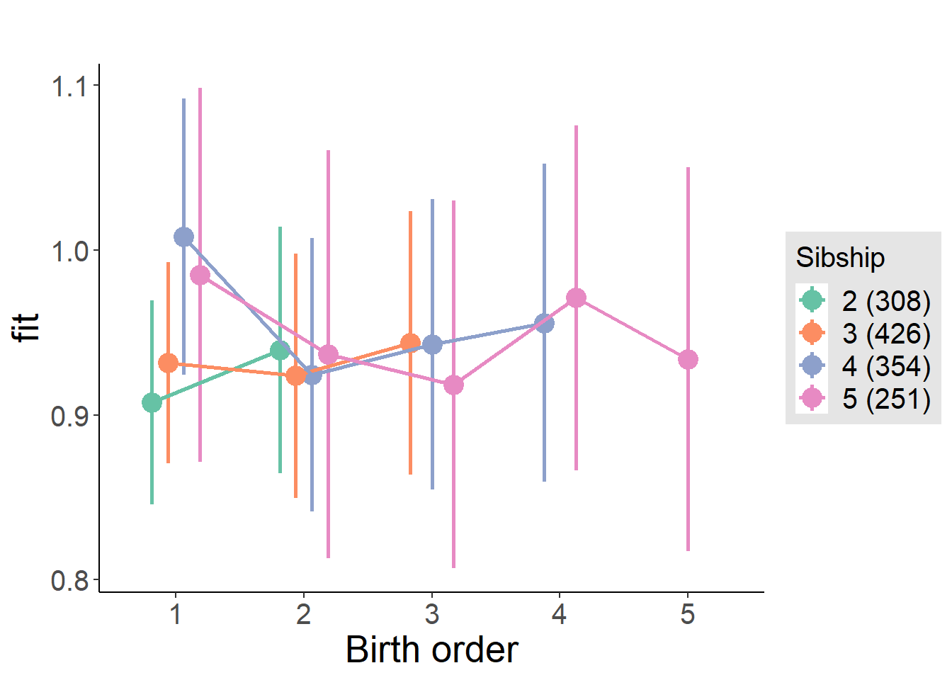
Model Comparison
###### Model 1 - Model 2
anova(m1_covariates_only, m2_birthorder_linear, m3_birthorder_nonlinear, m4_interaction)## refitting model(s) with ML (instead of REML)| Df | AIC | BIC | logLik | deviance | Chisq | Chi Df | Pr(>Chisq) |
|---|---|---|---|---|---|---|---|
| 10 | 387.2 | 439.2 | -183.6 | 367.2 | NA | NA | NA |
| 11 | 388.8 | 446 | -183.4 | 366.8 | 0.4035 | 1 | 0.5253 |
| 14 | 394 | 466.8 | -183 | 366 | 0.7669 | 3 | 0.8574 |
| 20 | 398.9 | 502.9 | -179.4 | 358.9 | 7.133 | 6 | 0.3087 |
Maternal pregnancy order
outcome_preg_m1 <- update(m2_birthorder_linear, data = birthorder %>%
mutate(sibling_count = sibling_count_uterus_preg_factor,
birth_order_nonlinear = birthorder_uterus_preg_factor,
birth_order = birthorder_uterus_preg,
count_birth_order = count_birthorder_uterus_preg
) %>%
filter(sibling_count != "1"))
compare_models_markdown(outcome_preg_m1)Basic Model
Model Summary
m1_covariates_only <- update(m2_birthorder_linear, formula = . ~ . - birth_order)
tidy(m1_covariates_only, conf.int = T, conf.level = 0.995)| effect | group | term | estimate | std.error | statistic | df | p.value | conf.low | conf.high |
|---|---|---|---|---|---|---|---|---|---|
| fixed | NA | (Intercept) | -0.3422 | 0.3223 | -1.062 | 1211 | 0.2885 | -1.247 | 0.5624 |
| fixed | NA | poly(age, 3, raw = TRUE)1 | 0.09807 | 0.03593 | 2.729 | 1209 | 0.006442 | -0.002799 | 0.1989 |
| fixed | NA | poly(age, 3, raw = TRUE)2 | -0.003374 | 0.00129 | -2.615 | 1207 | 0.009027 | -0.006996 | 0.0002474 |
| fixed | NA | poly(age, 3, raw = TRUE)3 | 0.00003564 | 0.00001481 | 2.406 | 1207 | 0.01628 | -0.000005942 | 0.00007722 |
| fixed | NA | male | 0.3741 | 0.05472 | 6.836 | 1214 | 0.00000000001283 | 0.2205 | 0.5277 |
| fixed | NA | sibling_count3 | 0.02237 | 0.02347 | 0.9533 | 1072 | 0.3407 | -0.04351 | 0.08825 |
| fixed | NA | sibling_count4 | 0.01799 | 0.02422 | 0.7425 | 1008 | 0.4579 | -0.05001 | 0.08598 |
| fixed | NA | sibling_count5 | 0.004768 | 0.02562 | 0.1861 | 974.3 | 0.8524 | -0.06715 | 0.07668 |
| ran_pars | mother_pidlink | sd__(Intercept) | 0.04332 | NA | NA | NA | NA | NA | NA |
| ran_pars | Residual | sd__Observation | 0.2816 | NA | NA | NA | NA | NA | NA |
Coefficient Plot
plot(allEffects(m1_covariates_only, confidence.level = 0.995))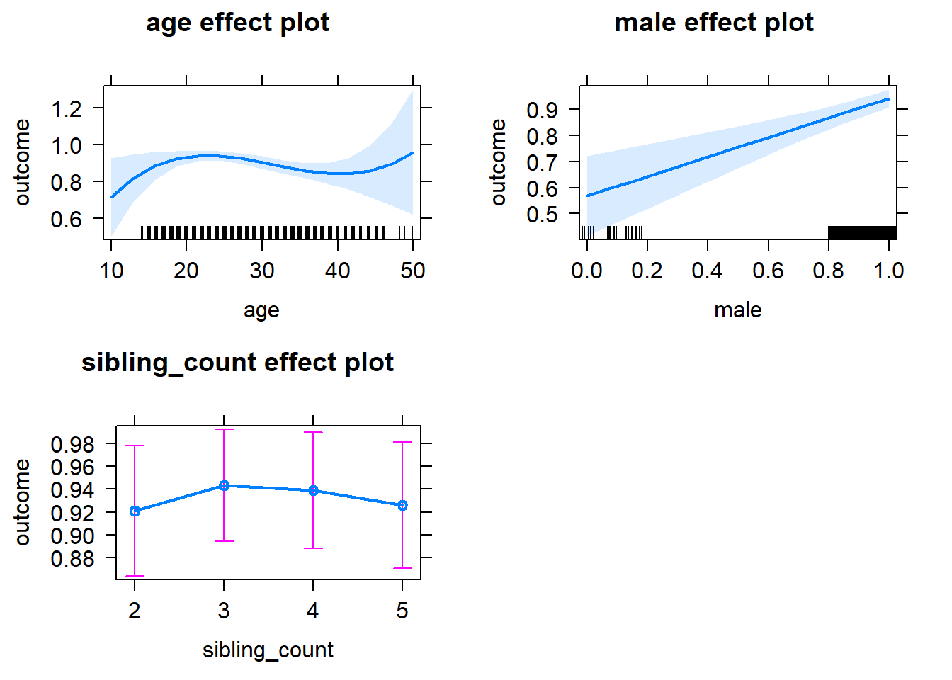
Add Birth Order Linear
Model Summary
tidy(m2_birthorder_linear, conf.int = T, conf.level = 0.995)| effect | group | term | estimate | std.error | statistic | df | p.value | conf.low | conf.high |
|---|---|---|---|---|---|---|---|---|---|
| fixed | NA | (Intercept) | -0.3446 | 0.3227 | -1.068 | 1210 | 0.2858 | -1.251 | 0.5613 |
| fixed | NA | birth_order | 0.001409 | 0.008034 | 0.1754 | 1215 | 0.8608 | -0.02114 | 0.02396 |
| fixed | NA | poly(age, 3, raw = TRUE)1 | 0.09816 | 0.03595 | 2.73 | 1208 | 0.006419 | -0.002758 | 0.1991 |
| fixed | NA | poly(age, 3, raw = TRUE)2 | -0.003379 | 0.001291 | -2.617 | 1206 | 0.008983 | -0.007002 | 0.0002454 |
| fixed | NA | poly(age, 3, raw = TRUE)3 | 0.0000357 | 0.00001482 | 2.409 | 1206 | 0.01617 | -0.000005907 | 0.00007732 |
| fixed | NA | male | 0.3738 | 0.05476 | 6.825 | 1213 | 0.00000000001384 | 0.22 | 0.5275 |
| fixed | NA | sibling_count3 | 0.02175 | 0.02375 | 0.9161 | 1080 | 0.3598 | -0.0449 | 0.08841 |
| fixed | NA | sibling_count4 | 0.01668 | 0.02536 | 0.6576 | 1027 | 0.511 | -0.05451 | 0.08786 |
| fixed | NA | sibling_count5 | 0.002659 | 0.02827 | 0.09404 | 1035 | 0.9251 | -0.0767 | 0.08201 |
| ran_pars | mother_pidlink | sd__(Intercept) | 0.04231 | NA | NA | NA | NA | NA | NA |
| ran_pars | Residual | sd__Observation | 0.2818 | NA | NA | NA | NA | NA | NA |
Coefficient Plot
plot_birthorder2(m2_birthorder_linear, separate = FALSE)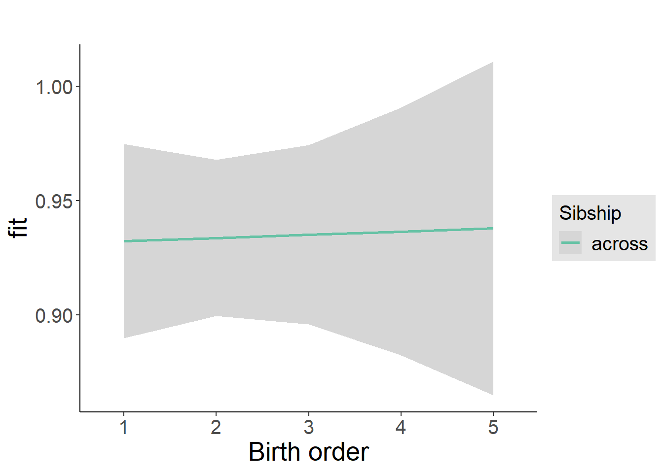
Add Birth Order Factor
Model Summary
m3_birthorder_nonlinear = update(m1_covariates_only, formula = . ~ . + birth_order_nonlinear)
tidy(m3_birthorder_nonlinear, conf.int = T, conf.level = 0.995)| effect | group | term | estimate | std.error | statistic | df | p.value | conf.low | conf.high |
|---|---|---|---|---|---|---|---|---|---|
| fixed | NA | (Intercept) | -0.3527 | 0.3228 | -1.092 | 1208 | 0.2749 | -1.259 | 0.5536 |
| fixed | NA | poly(age, 3, raw = TRUE)1 | 0.09996 | 0.03601 | 2.776 | 1206 | 0.005591 | -0.001123 | 0.201 |
| fixed | NA | poly(age, 3, raw = TRUE)2 | -0.003439 | 0.001293 | -2.66 | 1204 | 0.007928 | -0.007068 | 0.0001907 |
| fixed | NA | poly(age, 3, raw = TRUE)3 | 0.00003638 | 0.00001485 | 2.45 | 1204 | 0.01442 | -0.000005298 | 0.00007805 |
| fixed | NA | male | 0.3735 | 0.0548 | 6.815 | 1210 | 0.00000000001484 | 0.2196 | 0.5273 |
| fixed | NA | sibling_count3 | 0.02105 | 0.02421 | 0.8696 | 1103 | 0.3847 | -0.04691 | 0.08902 |
| fixed | NA | sibling_count4 | 0.01203 | 0.02577 | 0.4669 | 1040 | 0.6406 | -0.0603 | 0.08436 |
| fixed | NA | sibling_count5 | -0.001058 | 0.02876 | -0.03679 | 1034 | 0.9707 | -0.08178 | 0.07967 |
| fixed | NA | birth_order_nonlinear2 | -0.01748 | 0.01981 | -0.8823 | 1114 | 0.3778 | -0.07308 | 0.03813 |
| fixed | NA | birth_order_nonlinear3 | -0.001777 | 0.02426 | -0.07324 | 1141 | 0.9416 | -0.06988 | 0.06633 |
| fixed | NA | birth_order_nonlinear4 | 0.02172 | 0.032 | 0.6787 | 1201 | 0.4975 | -0.06811 | 0.1115 |
| fixed | NA | birth_order_nonlinear5 | -0.01202 | 0.04728 | -0.2541 | 1203 | 0.7994 | -0.1447 | 0.1207 |
| ran_pars | mother_pidlink | sd__(Intercept) | 0.03958 | NA | NA | NA | NA | NA | NA |
| ran_pars | Residual | sd__Observation | 0.2824 | NA | NA | NA | NA | NA | NA |
Coefficient Plot
plot_birthorder(m3_birthorder_nonlinear, separate = FALSE)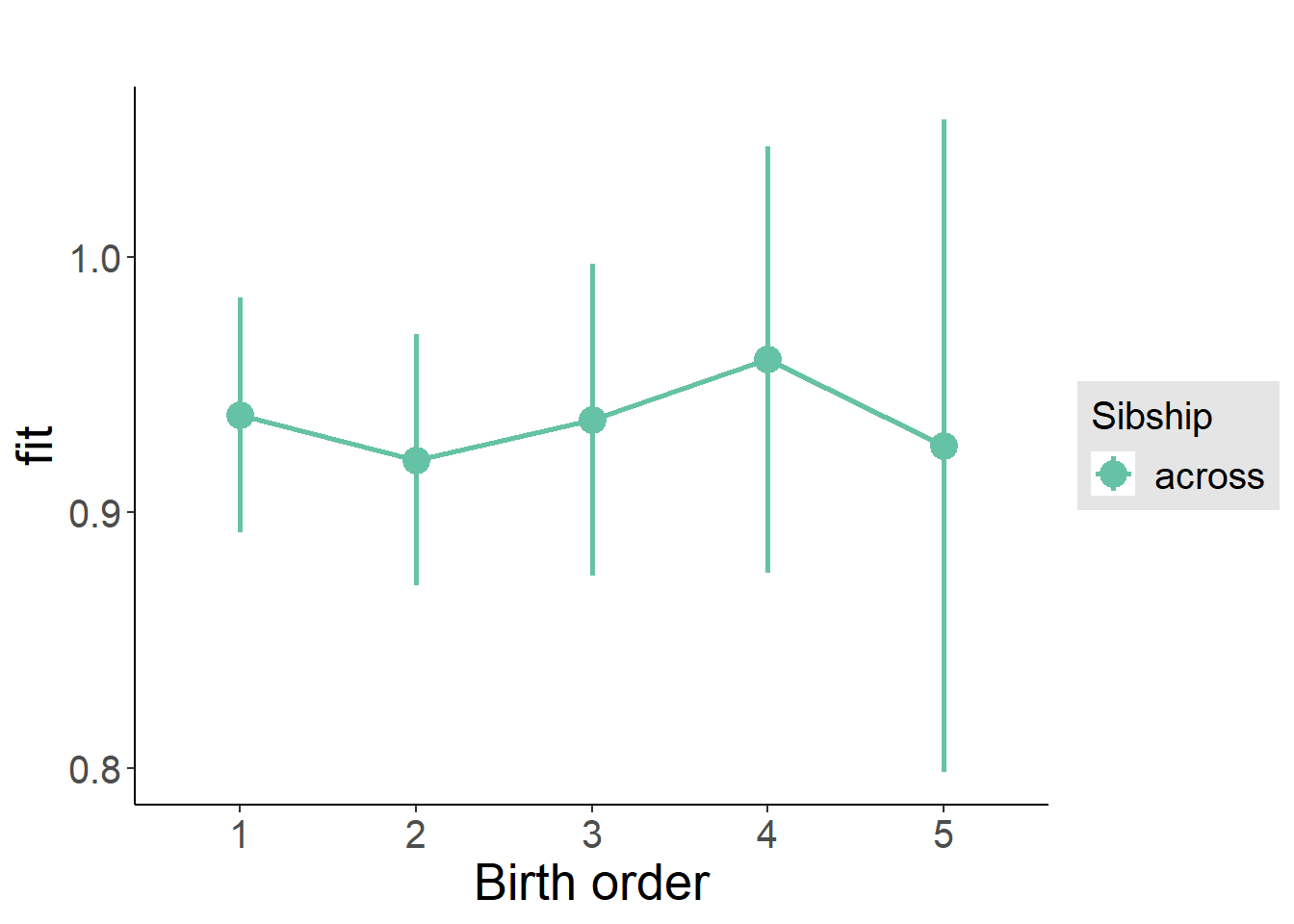
Add Interaction
Model Summary
m4_interaction = update(m3_birthorder_nonlinear, formula = . ~ . - birth_order_nonlinear - sibling_count + count_birth_order)
tidy(m4_interaction, conf.int = T, conf.level = 0.995)| effect | group | term | estimate | std.error | statistic | df | p.value | conf.low | conf.high |
|---|---|---|---|---|---|---|---|---|---|
| fixed | NA | (Intercept) | -0.3511 | 0.3243 | -1.083 | 1204 | 0.2791 | -1.261 | 0.5591 |
| fixed | NA | poly(age, 3, raw = TRUE)1 | 0.09842 | 0.03616 | 2.722 | 1202 | 0.006583 | -0.003075 | 0.1999 |
| fixed | NA | poly(age, 3, raw = TRUE)2 | -0.003363 | 0.001298 | -2.59 | 1200 | 0.009701 | -0.007007 | 0.0002811 |
| fixed | NA | poly(age, 3, raw = TRUE)3 | 0.0000353 | 0.00001491 | 2.368 | 1200 | 0.01805 | -0.000006546 | 0.00007714 |
| fixed | NA | male | 0.3774 | 0.055 | 6.861 | 1203 | 0.0000000000109 | 0.223 | 0.5318 |
| fixed | NA | count_birth_order2/2 | -0.009392 | 0.03705 | -0.2535 | 1151 | 0.7999 | -0.1134 | 0.0946 |
| fixed | NA | count_birth_order1/3 | 0.01043 | 0.03251 | 0.3207 | 1211 | 0.7485 | -0.08084 | 0.1017 |
| fixed | NA | count_birth_order2/3 | 0.02732 | 0.03557 | 0.7679 | 1211 | 0.4427 | -0.07254 | 0.1272 |
| fixed | NA | count_birth_order3/3 | 0.02145 | 0.03751 | 0.5718 | 1211 | 0.5676 | -0.08385 | 0.1267 |
| fixed | NA | count_birth_order1/4 | 0.01322 | 0.03691 | 0.3582 | 1211 | 0.7203 | -0.09038 | 0.1168 |
| fixed | NA | count_birth_order2/4 | -0.007754 | 0.03737 | -0.2075 | 1211 | 0.8357 | -0.1127 | 0.09715 |
| fixed | NA | count_birth_order3/4 | 0.02008 | 0.04177 | 0.4807 | 1211 | 0.6308 | -0.09717 | 0.1373 |
| fixed | NA | count_birth_order4/4 | 0.04027 | 0.04254 | 0.9467 | 1211 | 0.344 | -0.07913 | 0.1597 |
| fixed | NA | count_birth_order1/5 | 0.04257 | 0.04153 | 1.025 | 1211 | 0.3055 | -0.07401 | 0.1592 |
| fixed | NA | count_birth_order2/5 | -0.06287 | 0.04753 | -1.323 | 1210 | 0.1862 | -0.1963 | 0.07055 |
| fixed | NA | count_birth_order3/5 | -0.007506 | 0.04641 | -0.1617 | 1210 | 0.8715 | -0.1378 | 0.1228 |
| fixed | NA | count_birth_order4/5 | 0.01863 | 0.04687 | 0.3974 | 1211 | 0.6911 | -0.1129 | 0.1502 |
| fixed | NA | count_birth_order5/5 | -0.01039 | 0.04757 | -0.2184 | 1210 | 0.8271 | -0.1439 | 0.1231 |
| ran_pars | mother_pidlink | sd__(Intercept) | 0.03879 | NA | NA | NA | NA | NA | NA |
| ran_pars | Residual | sd__Observation | 0.2827 | NA | NA | NA | NA | NA | NA |
Coefficient Plot
plot_birthorder(m4_interaction)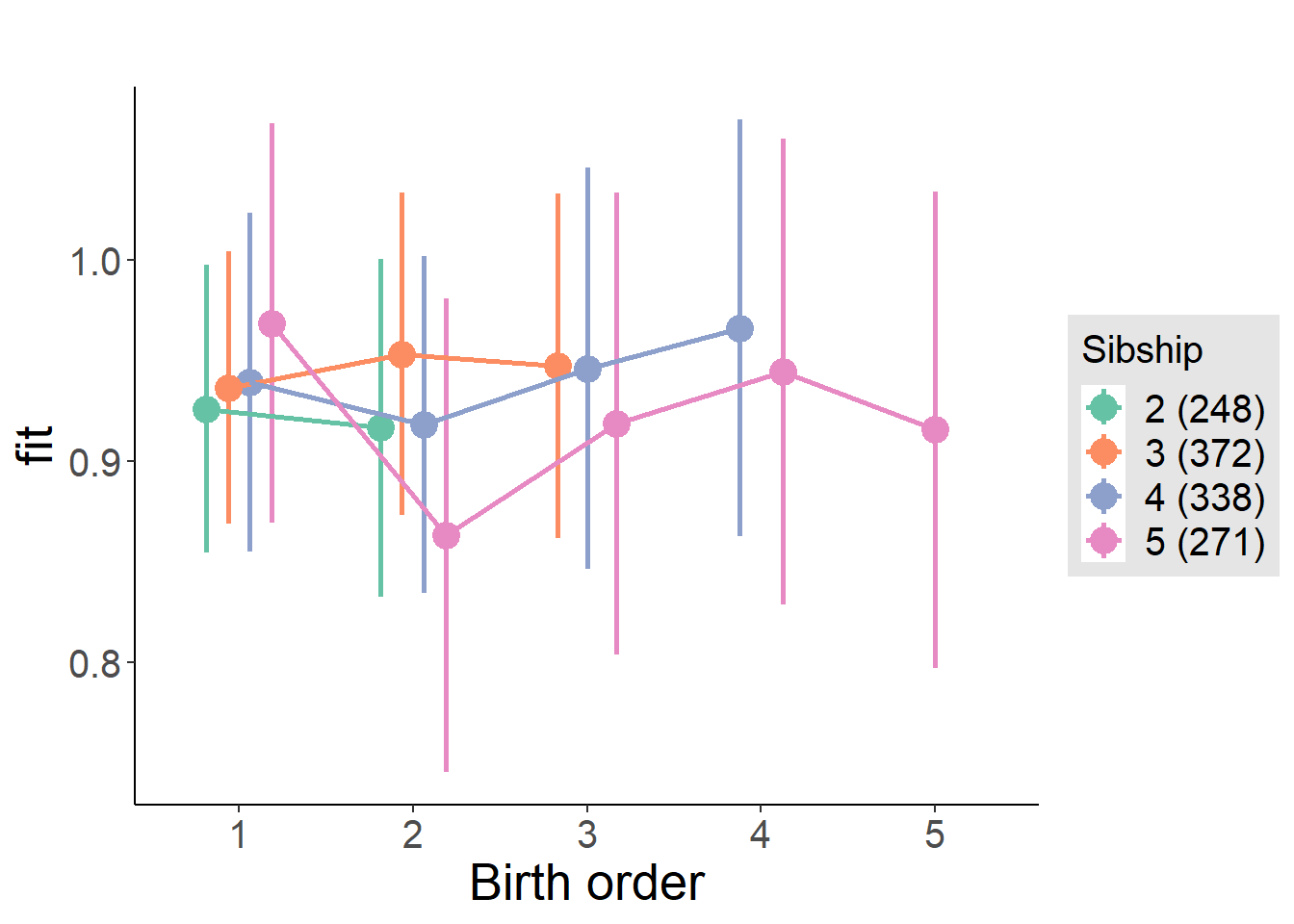
Model Comparison
###### Model 1 - Model 2
anova(m1_covariates_only, m2_birthorder_linear, m3_birthorder_nonlinear, m4_interaction)## refitting model(s) with ML (instead of REML)| Df | AIC | BIC | logLik | deviance | Chisq | Chi Df | Pr(>Chisq) |
|---|---|---|---|---|---|---|---|
| 10 | 413.3 | 464.4 | -196.6 | 393.3 | NA | NA | NA |
| 11 | 415.2 | 471.5 | -196.6 | 393.2 | 0.03241 | 1 | 0.8571 |
| 14 | 419.4 | 491 | -195.7 | 391.4 | 1.779 | 3 | 0.6195 |
| 20 | 427.4 | 529.7 | -193.7 | 387.4 | 4.005 | 6 | 0.676 |
Parental full sibling order
outcome_parental_m1 <- update(m2_birthorder_linear, data = birthorder %>%
mutate(sibling_count = sibling_count_genes_factor,
birth_order_nonlinear = birthorder_genes_factor,
birth_order = birthorder_genes,
count_birth_order = count_birthorder_genes
) %>%
filter(sibling_count != "1"))
compare_models_markdown(outcome_parental_m1)Basic Model
Model Summary
m1_covariates_only <- update(m2_birthorder_linear, formula = . ~ . - birth_order)
tidy(m1_covariates_only, conf.int = T, conf.level = 0.995)| effect | group | term | estimate | std.error | statistic | df | p.value | conf.low | conf.high |
|---|---|---|---|---|---|---|---|---|---|
| fixed | NA | (Intercept) | -0.1924 | 0.3072 | -0.6264 | 1320 | 0.5312 | -1.055 | 0.6699 |
| fixed | NA | poly(age, 3, raw = TRUE)1 | 0.09213 | 0.03404 | 2.706 | 1319 | 0.006894 | -0.003434 | 0.1877 |
| fixed | NA | poly(age, 3, raw = TRUE)2 | -0.003132 | 0.00122 | -2.567 | 1317 | 0.01037 | -0.006556 | 0.0002928 |
| fixed | NA | poly(age, 3, raw = TRUE)3 | 0.00003253 | 0.00001398 | 2.326 | 1317 | 0.02017 | -0.000006728 | 0.00007178 |
| fixed | NA | male | 0.2769 | 0.05175 | 5.351 | 1286 | 0.0000001036 | 0.1316 | 0.4222 |
| fixed | NA | sibling_count3 | 0.004604 | 0.02055 | 0.224 | 1120 | 0.8228 | -0.05309 | 0.06229 |
| fixed | NA | sibling_count4 | 0.02018 | 0.02195 | 0.9191 | 1080 | 0.3582 | -0.04145 | 0.08181 |
| fixed | NA | sibling_count5 | 0.01941 | 0.02495 | 0.7782 | 946.8 | 0.4366 | -0.05061 | 0.08944 |
| ran_pars | mother_pidlink | sd__(Intercept) | 0.04391 | NA | NA | NA | NA | NA | NA |
| ran_pars | Residual | sd__Observation | 0.2752 | NA | NA | NA | NA | NA | NA |
Coefficient Plot
plot(allEffects(m1_covariates_only, confidence.level = 0.995))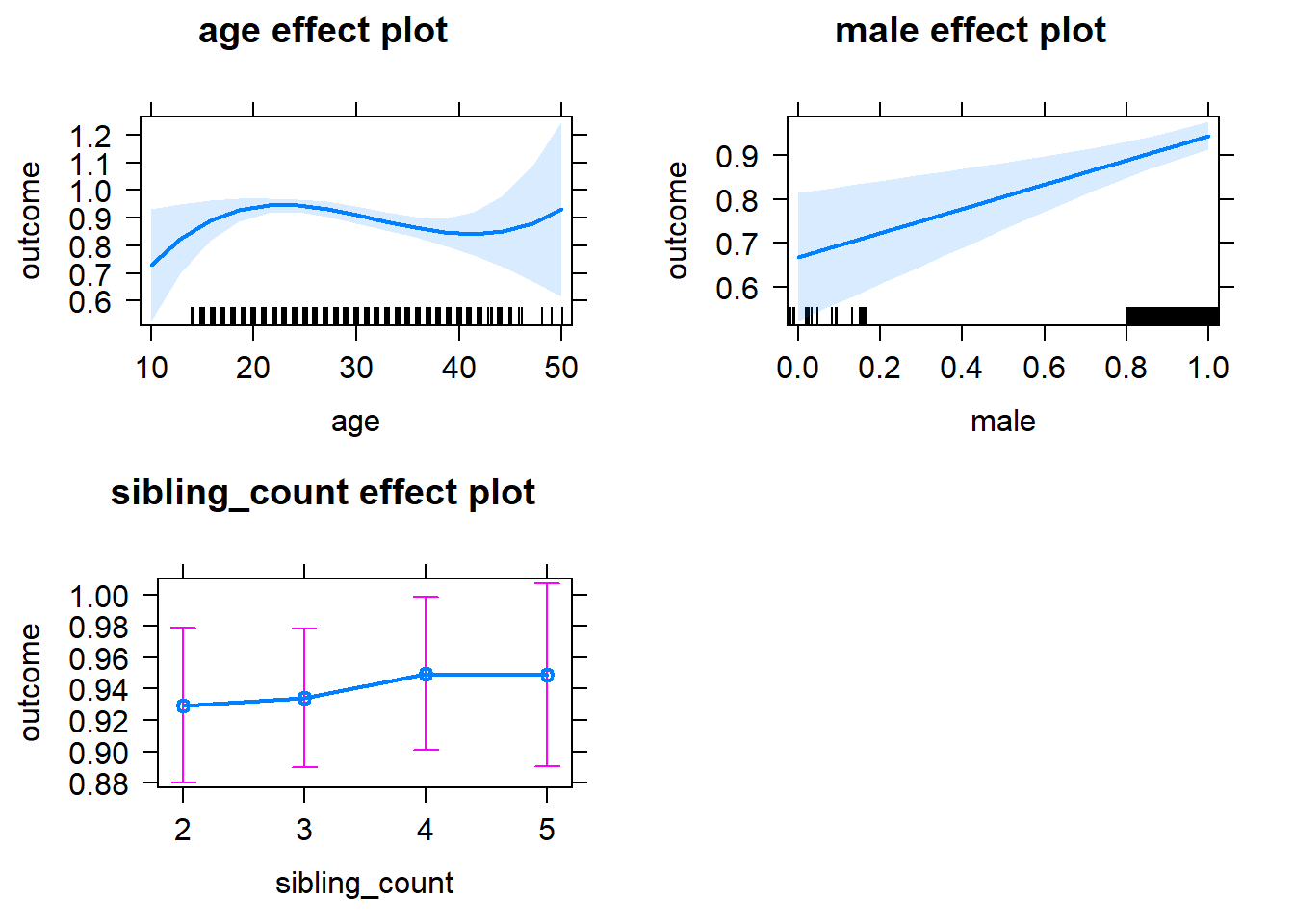
Add Birth Order Linear
Model Summary
tidy(m2_birthorder_linear, conf.int = T, conf.level = 0.995)| effect | group | term | estimate | std.error | statistic | df | p.value | conf.low | conf.high |
|---|---|---|---|---|---|---|---|---|---|
| fixed | NA | (Intercept) | -0.1862 | 0.3075 | -0.6056 | 1320 | 0.5449 | -1.049 | 0.677 |
| fixed | NA | birth_order | -0.004468 | 0.00797 | -0.5606 | 1309 | 0.5752 | -0.02684 | 0.0179 |
| fixed | NA | poly(age, 3, raw = TRUE)1 | 0.09211 | 0.03405 | 2.705 | 1318 | 0.006921 | -0.003479 | 0.1877 |
| fixed | NA | poly(age, 3, raw = TRUE)2 | -0.003127 | 0.00122 | -2.563 | 1316 | 0.0105 | -0.006553 | 0.0002984 |
| fixed | NA | poly(age, 3, raw = TRUE)3 | 0.0000324 | 0.00001399 | 2.316 | 1316 | 0.02071 | -0.000006871 | 0.00007167 |
| fixed | NA | male | 0.2767 | 0.05178 | 5.343 | 1287 | 0.0000001078 | 0.1313 | 0.422 |
| fixed | NA | sibling_count3 | 0.006499 | 0.02084 | 0.3119 | 1131 | 0.7552 | -0.052 | 0.06499 |
| fixed | NA | sibling_count4 | 0.02481 | 0.02346 | 1.058 | 1113 | 0.2905 | -0.04105 | 0.09067 |
| fixed | NA | sibling_count5 | 0.02672 | 0.02811 | 0.9505 | 1047 | 0.3421 | -0.05219 | 0.1056 |
| ran_pars | mother_pidlink | sd__(Intercept) | 0.04572 | NA | NA | NA | NA | NA | NA |
| ran_pars | Residual | sd__Observation | 0.275 | NA | NA | NA | NA | NA | NA |
Coefficient Plot
plot_birthorder2(m2_birthorder_linear, separate = FALSE)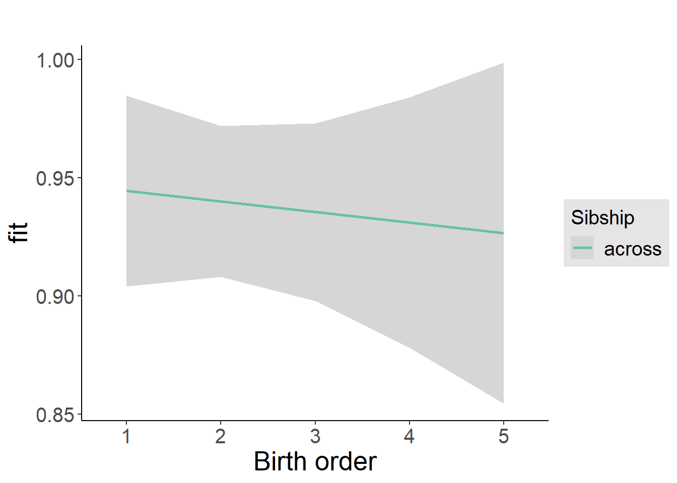
Add Birth Order Factor
Model Summary
m3_birthorder_nonlinear = update(m1_covariates_only, formula = . ~ . + birth_order_nonlinear)
tidy(m3_birthorder_nonlinear, conf.int = T, conf.level = 0.995)| effect | group | term | estimate | std.error | statistic | df | p.value | conf.low | conf.high |
|---|---|---|---|---|---|---|---|---|---|
| fixed | NA | (Intercept) | -0.1924 | 0.3076 | -0.6253 | 1317 | 0.5319 | -1.056 | 0.6712 |
| fixed | NA | poly(age, 3, raw = TRUE)1 | 0.0927 | 0.03411 | 2.718 | 1315 | 0.006659 | -0.003046 | 0.1884 |
| fixed | NA | poly(age, 3, raw = TRUE)2 | -0.003149 | 0.001222 | -2.576 | 1314 | 0.01009 | -0.00658 | 0.0002819 |
| fixed | NA | poly(age, 3, raw = TRUE)3 | 0.00003268 | 0.00001401 | 2.332 | 1314 | 0.01986 | -0.00000666 | 0.00007201 |
| fixed | NA | male | 0.2771 | 0.05184 | 5.346 | 1284 | 0.0000001064 | 0.1316 | 0.4226 |
| fixed | NA | sibling_count3 | 0.005655 | 0.02126 | 0.2661 | 1162 | 0.7902 | -0.05401 | 0.06532 |
| fixed | NA | sibling_count4 | 0.02156 | 0.02392 | 0.9013 | 1133 | 0.3676 | -0.04558 | 0.0887 |
| fixed | NA | sibling_count5 | 0.02512 | 0.02883 | 0.8714 | 1055 | 0.3837 | -0.0558 | 0.106 |
| fixed | NA | birth_order_nonlinear2 | -0.01438 | 0.01845 | -0.7793 | 1198 | 0.436 | -0.06617 | 0.03741 |
| fixed | NA | birth_order_nonlinear3 | -0.009366 | 0.02295 | -0.4081 | 1226 | 0.6833 | -0.07379 | 0.05506 |
| fixed | NA | birth_order_nonlinear4 | -0.002693 | 0.03149 | -0.08552 | 1295 | 0.9319 | -0.09108 | 0.0857 |
| fixed | NA | birth_order_nonlinear5 | -0.03263 | 0.04933 | -0.6616 | 1294 | 0.5084 | -0.1711 | 0.1058 |
| ran_pars | mother_pidlink | sd__(Intercept) | 0.04506 | NA | NA | NA | NA | NA | NA |
| ran_pars | Residual | sd__Observation | 0.2753 | NA | NA | NA | NA | NA | NA |
Coefficient Plot
plot_birthorder(m3_birthorder_nonlinear, separate = FALSE)
Add Interaction
Model Summary
m4_interaction = update(m3_birthorder_nonlinear, formula = . ~ . - birth_order_nonlinear - sibling_count + count_birth_order)
tidy(m4_interaction, conf.int = T, conf.level = 0.995)| effect | group | term | estimate | std.error | statistic | df | p.value | conf.low | conf.high |
|---|---|---|---|---|---|---|---|---|---|
| fixed | NA | (Intercept) | -0.2037 | 0.3092 | -0.6587 | 1311 | 0.5102 | -1.072 | 0.6642 |
| fixed | NA | poly(age, 3, raw = TRUE)1 | 0.09236 | 0.03433 | 2.69 | 1310 | 0.007226 | -0.004002 | 0.1887 |
| fixed | NA | poly(age, 3, raw = TRUE)2 | -0.003131 | 0.00123 | -2.545 | 1309 | 0.01105 | -0.006585 | 0.0003229 |
| fixed | NA | poly(age, 3, raw = TRUE)3 | 0.00003238 | 0.00001411 | 2.295 | 1308 | 0.0219 | -0.000007227 | 0.00007198 |
| fixed | NA | male | 0.2773 | 0.05191 | 5.341 | 1280 | 0.0000001092 | 0.1316 | 0.423 |
| fixed | NA | count_birth_order2/2 | 0.01851 | 0.03189 | 0.5805 | 1208 | 0.5617 | -0.07101 | 0.108 |
| fixed | NA | count_birth_order1/3 | 0.009038 | 0.02813 | 0.3213 | 1318 | 0.7481 | -0.06994 | 0.08801 |
| fixed | NA | count_birth_order2/3 | 0.003769 | 0.03138 | 0.1201 | 1318 | 0.9044 | -0.08431 | 0.09185 |
| fixed | NA | count_birth_order3/3 | 0.02768 | 0.03344 | 0.8276 | 1317 | 0.408 | -0.0662 | 0.1216 |
| fixed | NA | count_birth_order1/4 | 0.07038 | 0.0353 | 1.994 | 1318 | 0.04637 | -0.0287 | 0.1695 |
| fixed | NA | count_birth_order2/4 | -0.007811 | 0.0348 | -0.2244 | 1318 | 0.8225 | -0.1055 | 0.08988 |
| fixed | NA | count_birth_order3/4 | 0.01806 | 0.03662 | 0.4931 | 1316 | 0.622 | -0.08474 | 0.1209 |
| fixed | NA | count_birth_order4/4 | 0.03149 | 0.03871 | 0.8135 | 1317 | 0.4161 | -0.07717 | 0.1402 |
| fixed | NA | count_birth_order1/5 | 0.05928 | 0.04426 | 1.339 | 1318 | 0.1807 | -0.06495 | 0.1835 |
| fixed | NA | count_birth_order2/5 | 0.03278 | 0.04989 | 0.657 | 1318 | 0.5113 | -0.1073 | 0.1728 |
| fixed | NA | count_birth_order3/5 | -0.005393 | 0.04783 | -0.1127 | 1317 | 0.9102 | -0.1397 | 0.1289 |
| fixed | NA | count_birth_order4/5 | 0.03581 | 0.04598 | 0.7788 | 1317 | 0.4362 | -0.09325 | 0.1649 |
| fixed | NA | count_birth_order5/5 | 0.005418 | 0.04712 | 0.115 | 1317 | 0.9085 | -0.1269 | 0.1377 |
| ran_pars | mother_pidlink | sd__(Intercept) | 0.04845 | NA | NA | NA | NA | NA | NA |
| ran_pars | Residual | sd__Observation | 0.2748 | NA | NA | NA | NA | NA | NA |
Coefficient Plot
plot_birthorder(m4_interaction)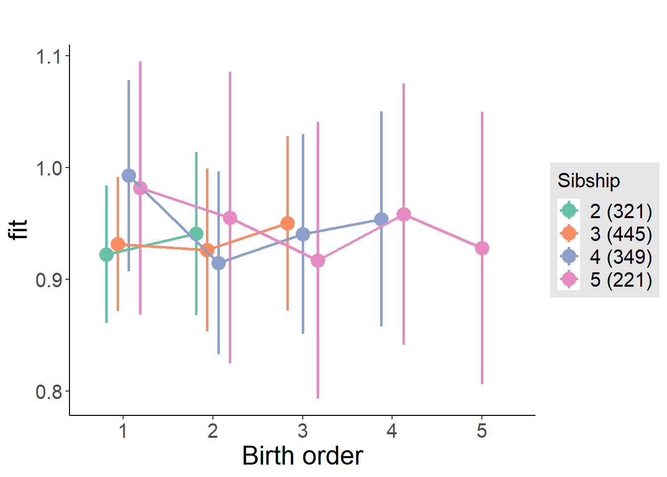
Model Comparison
###### Model 1 - Model 2
anova(m1_covariates_only, m2_birthorder_linear, m3_birthorder_nonlinear, m4_interaction)## refitting model(s) with ML (instead of REML)| Df | AIC | BIC | logLik | deviance | Chisq | Chi Df | Pr(>Chisq) |
|---|---|---|---|---|---|---|---|
| 10 | 389.2 | 441.2 | -184.6 | 369.2 | NA | NA | NA |
| 11 | 390.9 | 448.1 | -184.5 | 368.9 | 0.3117 | 1 | 0.5767 |
| 14 | 396.3 | 469 | -184.1 | 368.3 | 0.664 | 3 | 0.8816 |
| 20 | 402.8 | 506.8 | -181.4 | 362.8 | 5.434 | 6 | 0.4894 |
Compare birth order specifications
library(coefplot)
multiplot(outcome_naive_m1, outcome_preg_m1, outcome_uterus_m1, outcome_parental_m1, dodgeHeight = 0.6,
intercept = FALSE)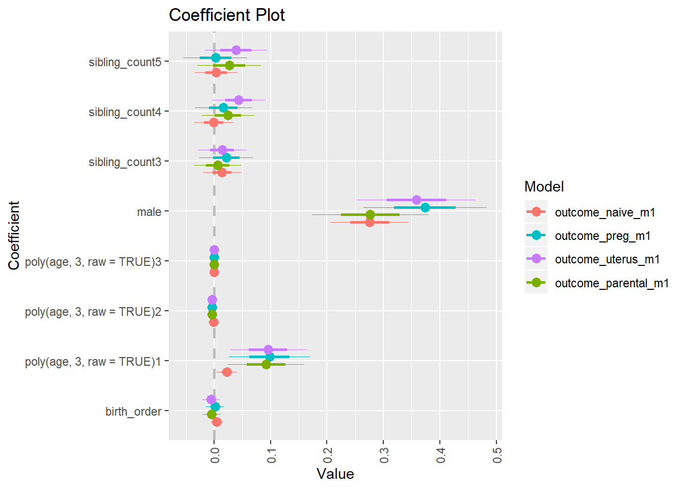
Multiplot Linear Birth Order Effect
Models
Intelligence = lmer(g_factor_2015_old ~ birthorder_genes + poly(age, 3, raw = TRUE) + male +
sibling_count_genes_factor +
(1 | mother_pidlink),
data = birthorder)`Educational Attainment` = lmer(years_of_education_z ~ birthorder_genes + poly(age, 3, raw = TRUE) + male +
sibling_count_genes_factor + (1 | mother_pidlink),
data = birthorder)Extraversion = lmer(big5_ext ~ birthorder_genes + poly(age, 3, raw = TRUE) + male +
sibling_count_genes_factor + (1 | mother_pidlink),
data = birthorder)Neuroticism = lmer(big5_neu ~ birthorder_genes + poly(age, 3, raw = TRUE) + male +
sibling_count_genes_factor + (1 | mother_pidlink),
data = birthorder)Conscientiousness = lmer(big5_con ~ birthorder_genes + poly(age, 3, raw = TRUE) + male +
sibling_count_genes_factor + (1 | mother_pidlink),
data = birthorder)Agreeableness = lmer(big5_agree ~ birthorder_genes + poly(age, 3, raw = TRUE) + male +
sibling_count_genes_factor + (1 | mother_pidlink),
data = birthorder)Openness = lmer(big5_open ~ birthorder_genes + poly(age, 3, raw = TRUE) + male +
sibling_count_genes_factor + (1 | mother_pidlink),
data = birthorder)RiskA = lmer(riskA ~ birthorder_genes + poly(age, 3, raw = TRUE) + male +
sibling_count_genes_factor + (1 | mother_pidlink),
data = birthorder)RiskB = lmer(riskB ~ birthorder_genes + poly(age, 3, raw = TRUE) + male +
sibling_count_genes_factor + (1 | mother_pidlink),
data = birthorder)Plot
x = multiplot(Intelligence, `Educational Attainment`, Agreeableness, Conscientiousness,
Extraversion, Neuroticism, Openness, RiskA, RiskB,
intercept = FALSE,
coefficients = c("birthorder_genes"),
outerCI = 2.807,
plot = F)
x = data.frame(x) %>%
mutate(Model = ifelse(Model == "`Educational Attainment`", "Educational Attainment", Model),
Model = ifelse(Model == "RiskA", "Risk Aversion A", Model),
Model = ifelse(Model == "RiskB", "Risk Aversion B", Model),
Model = as.factor(Model))
levels(x$Coefficient)birthorder_genes
x$Coefficient = ifelse(x$Coefficient == "birthorder_genes", "Birth order")
ggplot(x, aes(Model, Value)) +
scale_colour_brewer(palette = "Set2") +
geom_hline(yintercept = 0, size = 1.5) +
geom_rect(aes(xmin=0, xmax=Inf, ymin=-0.20, ymax=-0.07), fill = "lightgrey") +
geom_hline(yintercept = -.135, linetype = "dotted", size = 1.5) +
scale_x_discrete(limits=c("Risk Aversion B", "Risk Aversion A", "Openness", "Neuroticism",
"Extraversion", "Conscientiousness", "Agreeableness",
"Educational Attainment", "Intelligence")) +
geom_pointrange(data = x, mapping = aes(x=Model, y=Value, ymin=HighOuter, ymax=LowOuter,
color = Coefficient),
position = position_dodge(width=0.3), size = 1) +
coord_flip() +
labs(y = "Linear effect size", x = "Outcome") +
apatheme +
theme(text = element_text(size=25), axis.text.x = element_text(size = 20),
axis.text.y = element_text(size = 20), legend.position = "none")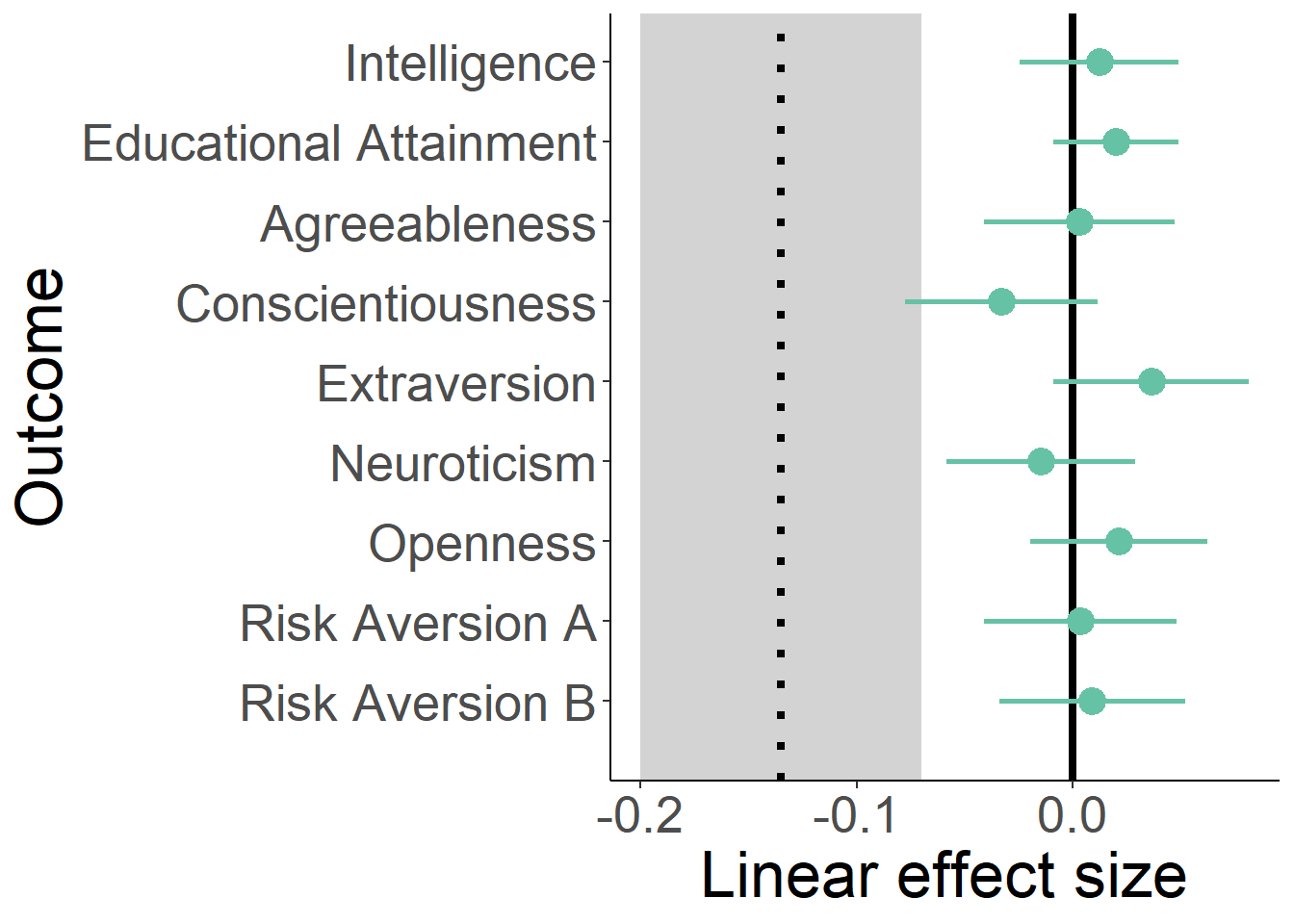
LS0tCnRpdGxlOiAiNF9hbmFseXNlc19yb2J1c3QiCmF1dGhvcjogIkxhdXJhIEJvdHpldCAmIFJ1YmVuIEFyc2xhbiIKb3V0cHV0OiBodG1sX2RvY3VtZW50CmVkaXRvcl9vcHRpb25zOiAKICBjaHVua19vdXRwdXRfdHlwZTogY29uc29sZQotLS0KIyA8c3BhbiBzdHlsZT0iY29sb3I6I0U1QzQ5NCI+Um9idXN0bmVzcyBBbmFseXNlczwvc3Bhbj4gey50YWJzZXR9CgojIyBIZWxwZXIKYGBge3IgaGVscGVyfQpzb3VyY2UoIjBfaGVscGVycy5SIikKb3B0c19jaHVuayRzZXQod2FybmluZyA9IEZBTFNFKQoKYGBgCgojIyBMb2FkIGRhdGEKYGBge3IgTG9hZCBEYXRhfQpiaXJ0aG9yZGVyID0gcmVhZFJEUygiZGF0YS9hbGxkYXRhX2JpcnRob3JkZXIucmRzIikKYGBgCgojIyBEYXRhIHByZXBhcmF0aW9ucwpgYGB7ciBkYXRhIHByZXBhcmF0aW9uc30KIyBGb3IgYW5hbHlzZXMgd2Ugd2FudCB0byBjbGVhbiB0aGUgZGF0YXNldCBhbmQgZ2V0IHJpZCBvZiBhbGwgdW5pbnRlcmVzdGluZyBkYXRhCmJpcnRob3JkZXIgPSBiaXJ0aG9yZGVyICU+JQogIGZpbHRlcighaXMubmEocGlkbGluaykpICU+JSAjIG5vIGluZGl2aWR1YWxzIHdobyBhcmUgb25seSBrbm93biBmcm9tIHRoZSBwcmVnbmFuY3kgZmlsZQogIGZpbHRlcihpcy5uYShsaWZlYmlydGhzKSB8IGxpZmViaXJ0aHMgPT0gMikgJT4lICMgcmVtb3ZlIDcgYW5kIDIgaW5kaXZpZHVhbHMgd2hvIGFyZSBrbm93biBhcyBzdGlsbGJpcnRoIG9yIG1pc2NhcnJpYWdlIGJ1dCBzdGlsbCBoYXZlIFBJRAogIHNlbGVjdCgtbGlmZWJpcnRocykgJT4lCiAgZmlsdGVyKCFpcy5uYShtb3RoZXJfcGlkbGluaykpICU+JQogIHNlbGVjdCgtZmF0aGVyX3BpZGxpbmspICU+JQogIGZpbHRlcihpcy5uYShhbnlfbXVsdGlwbGVfYmlydGgpIHwgYW55X211bHRpcGxlX2JpcnRoICE9IDEpICU+JSAjIHJlbW92ZSBmYW1pbGllcyB3aXRoIHR3aW5zL3RyaXBsZXRzLy4uCiAgZmlsdGVyKCFpcy5uYShiaXJ0aG9yZGVyX25haXZlKSkgJT4lCiAgc2VsZWN0KC1zdGFydHNfd2l0aCgiYWdlXyIpLCAtd2F2ZSwgLWFueV9tdWx0aXBsZV9iaXJ0aCwgLW11bHRpcGxlX2JpcnRoKSAlPiUKICBtdXRhdGUobW9uZXlfc3BlbnRfc21va2luZ19sb2cgPSBpZl9lbHNlKGlzLm5hKG1vbmV5X3NwZW50X3Ntb2tpbmdfbG9nKSAmIGV2ZXJfc21va2VkID09IDAsIDAsIG1vbmV5X3NwZW50X3Ntb2tpbmdfbG9nKSwKICAgICAgICAgYW1vdW50ID0gaWZfZWxzZShpcy5uYShhbW91bnQpICYgZXZlcl9zbW9rZWQgPT0gMCwgMCwgYW1vdW50KSwKICAgICAgICAgYW1vdW50X3N0aWxsX3Ntb2tlcnMgPSBpZl9lbHNlKGlzLm5hKGFtb3VudF9zdGlsbF9zbW9rZXJzKSAmICBzdGlsbF9zbW9raW5nID09IDAsIDAsIGFtb3VudF9zdGlsbF9zbW9rZXJzKSwKICAgICAgICAgYmlydGh5ZWFyID0gbHVicmlkYXRlOjp5ZWFyKGJpcnRoZGF0ZSkpCgojIHJlY29kZSBGYWN0b3IgVmFyaWFibGUgYXMgRHVtbXkgVmFyaWFibGUKYmlydGhvcmRlciA9IGxlZnRfam9pbihiaXJ0aG9yZGVyLAogICAgICAgICAgICAgICAgICAgICAgICAgICAgICAgIGJpcnRob3JkZXIgJT4lCiAgICAgICAgICAgICAgICAgICAgICAgICAgICAgICAgICBmaWx0ZXIoIWlzLm5hKENhdGVnb3J5KSkgJT4lCiAgICAgICAgICAgICAgICAgICAgICAgICAgICAgICAgICBtdXRhdGUodmFyID0gMSkgJT4lCiAgICAgICAgICAgICAgICAgICAgICAgICAgICAgICAgICBzZWxlY3QocGlkbGluaywgQ2F0ZWdvcnksIHZhcikgJT4lCiAgICAgICAgICAgICAgICAgICAgICAgICAgICAgICAgICBzcHJlYWQoQ2F0ZWdvcnksIHZhciwgZmlsbCA9IDAsIHNlcCA9ICJfIiksIGJ5ID0gInBpZGxpbmsiKSAlPiUKICBzZWxlY3QoLUNhdGVnb3J5KQoKIyByZWNvZGUgRmFjdG9yIFZhcmlhYmxlIGFzIER1bW15IFZhcmlhYmxlCmJpcnRob3JkZXIgPSBsZWZ0X2pvaW4oYmlydGhvcmRlciwKICAgICAgICAgICAgICAgICAgICAgICAgICAgICAgICBiaXJ0aG9yZGVyICU+JQogICAgICAgICAgICAgICAgICAgICAgICAgICAgICAgICAgZmlsdGVyKCFpcy5uYShTZWN0b3IpKSAlPiUKICAgICAgICAgICAgICAgICAgICAgICAgICAgICAgICAgIG11dGF0ZSh2YXIgPSAxKSAlPiUKICAgICAgICAgICAgICAgICAgICAgICAgICAgICAgICAgIHNlbGVjdChwaWRsaW5rLCBTZWN0b3IsIHZhcikgJT4lCiAgICAgICAgICAgICAgICAgICAgICAgICAgICAgICAgICBzcHJlYWQoU2VjdG9yLCB2YXIsIGZpbGwgPSAwLCBzZXAgPSAiXyIpLCBieSA9ICJwaWRsaW5rIikgJT4lCiAgc2VsZWN0KC1TZWN0b3IpCgoKIyMjIFZhcmlhYmxlcwpiaXJ0aG9yZGVyID0gYmlydGhvcmRlciAlPiUKICBtdXRhdGUoCiAgICAjIGNlbnRlciB2YXJpYWJsZXMgdGhhdCBhcmUgdXNlZCBmb3IgYW5hbHlzaXMKICBnX2ZhY3Rvcl8yMDE1X29sZCA9IHNjYWxlKGdfZmFjdG9yXzIwMTVfb2xkKSwKICBnX2ZhY3Rvcl8yMDE1X3lvdW5nID0gc2NhbGUoZ19mYWN0b3JfMjAxNV95b3VuZyksCiAgZ19mYWN0b3JfMjAwN19vbGQgPSBzY2FsZShnX2ZhY3Rvcl8yMDA3X29sZCksCiAgZ19mYWN0b3JfMjAwN195b3VuZyA9IHNjYWxlKGdfZmFjdG9yXzIwMDdfeW91bmcpLAogIHJhdmVuXzIwMTVfb2xkID0gc2NhbGUocmF2ZW5fMjAxNV9vbGQpLAogIG1hdGhfMjAxNV9vbGQgPSBzY2FsZShtYXRoXzIwMTVfb2xkKSwKICBjb3VudF9iYWNrd2FyZHMgPSBzY2FsZShjb3VudF9iYWNrd2FyZHMpLAogIHJhdmVuXzIwMTVfeW91bmcgPSBzY2FsZShyYXZlbl8yMDE1X3lvdW5nKSwKICBtYXRoXzIwMTVfeW91bmcgPSBzY2FsZShtYXRoXzIwMTVfeW91bmcpLAogIHdvcmRzX3JlbWVtYmVyZWRfYXZnID0gc2NhbGUod29yZHNfcmVtZW1iZXJlZF9hdmcpLAogIHdvcmRzX2ltbWVkaWF0ZSA9IHNjYWxlKHdvcmRzX2ltbWVkaWF0ZSksCiAgd29yZHNfZGVsYXllZCA9IHNjYWxlKHdvcmRzX2RlbGF5ZWQpLAogIGFkYXB0aXZlX251bWJlcmluZyA9IHNjYWxlKGFkYXB0aXZlX251bWJlcmluZyksCiAgcmF2ZW5fMjAwN19vbGQgPSBzY2FsZShyYXZlbl8yMDA3X29sZCksCiAgbWF0aF8yMDA3X29sZCA9IHNjYWxlKG1hdGhfMjAwN19vbGQpLAogIHJhdmVuXzIwMDdfeW91bmcgPSBzY2FsZShyYXZlbl8yMDA3X3lvdW5nKSwKICBtYXRoXzIwMDdfeW91bmcgPSBzY2FsZShtYXRoXzIwMDdfeW91bmcpLAogIHJpc2tBID0gc2NhbGUocmlza0EpLAogIHJpc2tCID0gc2NhbGUocmlza0IpLAogIHllYXJzX29mX2VkdWNhdGlvbl96ID0gc2NhbGUoeWVhcnNfb2ZfZWR1Y2F0aW9uKSwKICBUb3RhbF9zY29yZV9oaWdoZXN0X3ogPSBzY2FsZShUb3RhbF9zY29yZV9oaWdoZXN0KSwKICB3YWdlX2xhc3RfbW9udGhfeiA9IHNjYWxlKHdhZ2VfbGFzdF9tb250aF9sb2cpLAogIHdhZ2VfbGFzdF95ZWFyX3ogPSBzY2FsZSh3YWdlX2xhc3RfeWVhcl9sb2cpLAogIGJpZzVfZXh0ID0gc2NhbGUoYmlnNV9leHQpLAogIGJpZzVfY29uID0gc2NhbGUoYmlnNV9jb24pLAogIGJpZzVfYWdyZWUgPSBzY2FsZShiaWc1X2FncmVlKSwKICBiaWc1X29wZW4gPSBzY2FsZShiaWc1X29wZW4pLAogIGJpZzVfbmV1ID0gc2NhbGUoYmlnNV9uZXUpLAogIGF0dGVuZGVkX3NjaG9vbCA9IGFzLmludGVnZXIoYXR0ZW5kZWRfc2Nob29sKSwKICBhdHRlbmRlZF9zY2hvb2wgPSBpZmVsc2UoYXR0ZW5kZWRfc2Nob29sID09IDEsIDAsCiAgICAgICAgICAgICAgICAgICAgICAgICAgIGlmZWxzZShhdHRlbmRlZF9zY2hvb2wgPT0gMiwgMSwgTkEpKSkKCiMjIyBCaXJ0aG9yZGVyIGFuZCBTaWJsaW5nIENvdW50CmJpcnRob3JkZXIgPSBiaXJ0aG9yZGVyICU+JSAKICBtdXRhdGUoCiMgYmlydGhvcmRlciBhcyBmYWN0b3JzIHdpdGggbGV2ZWxzIG9mIDEsIDIsIDMsIDQsIDUsCiAgICBiaXJ0aG9yZGVyX25haXZlX2ZhY3RvciA9IGFzLmNoYXJhY3RlcihiaXJ0aG9yZGVyX25haXZlKSwKICAgIGJpcnRob3JkZXJfbmFpdmVfZmFjdG9yID0gaWZlbHNlKGJpcnRob3JkZXJfbmFpdmUgPiA1LCBOQSwKICAgICAgICAgICAgICAgICAgICAgICAgICAgICAgICAgICAgICAgICAgICBiaXJ0aG9yZGVyX25haXZlX2ZhY3RvciksCiAgICBiaXJ0aG9yZGVyX25haXZlX2ZhY3RvciA9IGZhY3RvcihiaXJ0aG9yZGVyX25haXZlX2ZhY3RvciwgCiAgICAgICAgICAgICAgICAgICAgICAgICAgICAgICAgICAgICAgICAgICAgbGV2ZWxzID0gYygiMSIsIjIiLCIzIiwiNCIsIjUiKSksCiAgICBzaWJsaW5nX2NvdW50X25haXZlX2ZhY3RvciA9IGFzLmNoYXJhY3RlcihzaWJsaW5nX2NvdW50X25haXZlKSwKICAgIHNpYmxpbmdfY291bnRfbmFpdmVfZmFjdG9yID0gaWZlbHNlKHNpYmxpbmdfY291bnRfbmFpdmUgPiA1LCBOQSwKICAgICAgICAgICAgICAgICAgICAgICAgICAgICAgICAgICAgICAgICAgICAgICBzaWJsaW5nX2NvdW50X25haXZlX2ZhY3RvciksCiAgICBzaWJsaW5nX2NvdW50X25haXZlX2ZhY3RvciA9IGZhY3RvcihzaWJsaW5nX2NvdW50X25haXZlX2ZhY3RvciwgCiAgICAgICAgICAgICAgICAgICAgICAgICAgICAgICAgICAgICAgICAgICAgICAgbGV2ZWxzID0gYygiMiIsIjMiLCI0IiwiNSIpKSwKCiAgICBiaXJ0aG9yZGVyX3V0ZXJ1c19hbGl2ZV9mYWN0b3IgPSBhcy5jaGFyYWN0ZXIoYmlydGhvcmRlcl91dGVydXNfYWxpdmUpLAogICAgYmlydGhvcmRlcl91dGVydXNfYWxpdmVfZmFjdG9yID0gaWZlbHNlKGJpcnRob3JkZXJfdXRlcnVzX2FsaXZlID4gNSwgTkEsCiAgICAgICAgICAgICAgICAgICAgICAgICAgICAgICAgICAgICAgICAgICAgYmlydGhvcmRlcl91dGVydXNfYWxpdmVfZmFjdG9yKSwKICAgIGJpcnRob3JkZXJfdXRlcnVzX2FsaXZlX2ZhY3RvciA9IGZhY3RvcihiaXJ0aG9yZGVyX3V0ZXJ1c19hbGl2ZV9mYWN0b3IsIAogICAgICAgICAgICAgICAgICAgICAgICAgICAgICAgICAgICAgICAgICAgIGxldmVscyA9IGMoIjEiLCIyIiwiMyIsIjQiLCI1IikpLAogICAgc2libGluZ19jb3VudF91dGVydXNfYWxpdmVfZmFjdG9yID0gYXMuY2hhcmFjdGVyKHNpYmxpbmdfY291bnRfdXRlcnVzX2FsaXZlKSwKICAgIHNpYmxpbmdfY291bnRfdXRlcnVzX2FsaXZlX2ZhY3RvciA9IGlmZWxzZShzaWJsaW5nX2NvdW50X3V0ZXJ1c19hbGl2ZSA+IDUsIE5BLAogICAgICAgICAgICAgICAgICAgICAgICAgICAgICAgICAgICAgICAgICAgICAgIHNpYmxpbmdfY291bnRfdXRlcnVzX2FsaXZlX2ZhY3RvciksCiAgICBzaWJsaW5nX2NvdW50X3V0ZXJ1c19hbGl2ZV9mYWN0b3IgPSBmYWN0b3Ioc2libGluZ19jb3VudF91dGVydXNfYWxpdmVfZmFjdG9yLCAKICAgICAgICAgICAgICAgICAgICAgICAgICAgICAgICAgICAgICAgICAgICAgICBsZXZlbHMgPSBjKCIyIiwiMyIsIjQiLCI1IikpLAogICAgYmlydGhvcmRlcl91dGVydXNfcHJlZ19mYWN0b3IgPSBhcy5jaGFyYWN0ZXIoYmlydGhvcmRlcl91dGVydXNfcHJlZyksCiAgICBiaXJ0aG9yZGVyX3V0ZXJ1c19wcmVnX2ZhY3RvciA9IGlmZWxzZShiaXJ0aG9yZGVyX3V0ZXJ1c19wcmVnID4gNSwgTkEsCiAgICAgICAgICAgICAgICAgICAgICAgICAgICAgICAgICAgICAgICAgICBiaXJ0aG9yZGVyX3V0ZXJ1c19wcmVnX2ZhY3RvciksCiAgICBiaXJ0aG9yZGVyX3V0ZXJ1c19wcmVnX2ZhY3RvciA9IGZhY3RvcihiaXJ0aG9yZGVyX3V0ZXJ1c19wcmVnX2ZhY3RvciwKICAgICAgICAgICAgICAgICAgICAgICAgICAgICAgICAgICAgICAgICAgIGxldmVscyA9IGMoIjEiLCIyIiwiMyIsIjQiLCI1IikpLAogICAgc2libGluZ19jb3VudF91dGVydXNfcHJlZ19mYWN0b3IgPSBhcy5jaGFyYWN0ZXIoc2libGluZ19jb3VudF91dGVydXNfcHJlZyksCiAgICBzaWJsaW5nX2NvdW50X3V0ZXJ1c19wcmVnX2ZhY3RvciA9IGlmZWxzZShzaWJsaW5nX2NvdW50X3V0ZXJ1c19wcmVnID4gNSwgTkEsCiAgICAgICAgICAgICAgICAgICAgICAgICAgICAgICAgICAgICAgICAgICAgICBzaWJsaW5nX2NvdW50X3V0ZXJ1c19wcmVnX2ZhY3RvciksCiAgICBzaWJsaW5nX2NvdW50X3V0ZXJ1c19wcmVnX2ZhY3RvciA9IGZhY3RvcihzaWJsaW5nX2NvdW50X3V0ZXJ1c19wcmVnX2ZhY3RvciwgCiAgICAgICAgICAgICAgICAgICAgICAgICAgICAgICAgICAgICAgICAgICAgICBsZXZlbHMgPSBjKCIyIiwiMyIsIjQiLCI1IikpLAogICAgYmlydGhvcmRlcl9nZW5lc19mYWN0b3IgPSBhcy5jaGFyYWN0ZXIoYmlydGhvcmRlcl9nZW5lcyksCiAgICBiaXJ0aG9yZGVyX2dlbmVzX2ZhY3RvciA9IGlmZWxzZShiaXJ0aG9yZGVyX2dlbmVzID41ICwgTkEsIGJpcnRob3JkZXJfZ2VuZXNfZmFjdG9yKSwKICAgIGJpcnRob3JkZXJfZ2VuZXNfZmFjdG9yID0gZmFjdG9yKGJpcnRob3JkZXJfZ2VuZXNfZmFjdG9yLCAKICAgICAgICAgICAgICAgICAgICAgICAgICAgICAgICAgICAgIGxldmVscyA9IGMoIjEiLCIyIiwiMyIsIjQiLCI1IikpLAogICAgc2libGluZ19jb3VudF9nZW5lc19mYWN0b3IgPSBhcy5jaGFyYWN0ZXIoc2libGluZ19jb3VudF9nZW5lcyksCiAgICBzaWJsaW5nX2NvdW50X2dlbmVzX2ZhY3RvciA9IGlmZWxzZShzaWJsaW5nX2NvdW50X2dlbmVzID41ICwgTkEsCiAgICAgICAgICAgICAgICAgICAgICAgICAgICAgICAgICAgICAgICBzaWJsaW5nX2NvdW50X2dlbmVzX2ZhY3RvciksCiAgICBzaWJsaW5nX2NvdW50X2dlbmVzX2ZhY3RvciA9IGZhY3RvcihzaWJsaW5nX2NvdW50X2dlbmVzX2ZhY3RvciwgCiAgICAgICAgICAgICAgICAgICAgICAgICAgICAgICAgICAgICAgICBsZXZlbHMgPSBjKCIyIiwiMyIsIjQiLCI1IikpLAogICAgIyBpbnRlcmFjdGlvbiBiaXJ0aG9yZGVyICogc2libGluZ2NvdXQgZm9yIGVhY2ggYmlydGhvcmRlcgogICAgY291bnRfYmlydGhvcmRlcl9uYWl2ZSA9CiAgICAgIGZhY3RvcihzdHJfcmVwbGFjZShhcy5jaGFyYWN0ZXIoaW50ZXJhY3Rpb24oYmlydGhvcmRlcl9uYWl2ZV9mYWN0b3IsICAgICAgICAgICAgICAgICAgICAgICAgICAgICAgICAgICAgICAgICAgICAgICAgICAgICAgICAgICAgICBzaWJsaW5nX2NvdW50X25haXZlX2ZhY3RvcikpLAogICAgICAgICAgICAgICAgICAgICAgICAiXFwuIiwgIi8iKSwKICAgICAgICAgICAgICAgICAgICAgICAgICAgICAgICAgICAgICAgICAgIGxldmVscyA9ICAgYygiMS8yIiwiMi8yIiwgIjEvMyIsICAiMi8zIiwKICAgICAgICAgICAgICAgICAgICAgICAgICAgICAgICAgICAgICAgICAgICAgICAgICAgICAgICAiMy8zIiwgIjEvNCIsICIyLzQiLCAiMy80IiwgIjQvNCIsCiAgICAgICAgICAgICAgICAgICAgICAgICAgICAgICAgICAgICAgICAgICAgICAgICAgICAgICAgIjEvNSIsICIyLzUiLCAiMy81IiwgIjQvNSIsCiAgICAgICAgICAgICAgICAgICAgICAgICAgICAgICAgICAgICAgICAgICAgICAgICAgICAgICAgIjUvNSIpKSwKICAgIGNvdW50X2JpcnRob3JkZXJfdXRlcnVzX2FsaXZlID0KICAgICAgZmFjdG9yKHN0cl9yZXBsYWNlKGFzLmNoYXJhY3RlcihpbnRlcmFjdGlvbihiaXJ0aG9yZGVyX3V0ZXJ1c19hbGl2ZV9mYWN0b3IsICAgICAgICAgICAgICAgICAgICAgICAgICAgICAgICAgICAgICAgICAgICAgICAgICAgICAgICAgICAgICBzaWJsaW5nX2NvdW50X3V0ZXJ1c19hbGl2ZV9mYWN0b3IpKSwKICAgICAgICAgICAgICAgICAgICAgICAgIlxcLiIsICIvIiksCiAgICAgICAgICAgICAgICAgICAgICAgICAgICAgICAgICAgICAgICAgICBsZXZlbHMgPSAgIGMoIjEvMiIsIjIvMiIsICIxLzMiLCAgIjIvMyIsCiAgICAgICAgICAgICAgICAgICAgICAgICAgICAgICAgICAgICAgICAgICAgICAgICAgICAgICAgIjMvMyIsICIxLzQiLCAiMi80IiwgIjMvNCIsICI0LzQiLAogICAgICAgICAgICAgICAgICAgICAgICAgICAgICAgICAgICAgICAgICAgICAgICAgICAgICAgICIxLzUiLCAiMi81IiwgIjMvNSIsICI0LzUiLCAiNS81IikpLAogICAgY291bnRfYmlydGhvcmRlcl91dGVydXNfcHJlZyA9CiAgICAgIGZhY3RvcihzdHJfcmVwbGFjZShhcy5jaGFyYWN0ZXIoaW50ZXJhY3Rpb24oYmlydGhvcmRlcl91dGVydXNfcHJlZ19mYWN0b3IsICAgICAgICAgICAgICAgICAgICAgICAgICAgICAgICAgICAgICAgICAgICAgICAgICAgICAgICAgICAgICBzaWJsaW5nX2NvdW50X3V0ZXJ1c19wcmVnX2ZhY3RvcikpLCAKICAgICAgICAgICAgICAgICAgICAgICAgICJcXC4iLCAiLyIpLAogICAgICAgICAgICAgICAgICAgICAgICAgICAgICAgICAgICAgICAgICAgbGV2ZWxzID0gICBjKCIxLzIiLCIyLzIiLCAiMS8zIiwgICIyLzMiLAogICAgICAgICAgICAgICAgICAgICAgICAgICAgICAgICAgICAgICAgICAgICAgICAgICAgICAgICIzLzMiLCAiMS80IiwgIjIvNCIsICIzLzQiLCAiNC80IiwKICAgICAgICAgICAgICAgICAgICAgICAgICAgICAgICAgICAgICAgICAgICAgICAgICAgICAgICAiMS81IiwgIjIvNSIsICIzLzUiLCAiNC81IiwgIjUvNSIpKSwKICAgIGNvdW50X2JpcnRob3JkZXJfZ2VuZXMgPQogICAgICBmYWN0b3Ioc3RyX3JlcGxhY2UoYXMuY2hhcmFjdGVyKGludGVyYWN0aW9uKGJpcnRob3JkZXJfZ2VuZXNfZmFjdG9yLCAgICAgICAgICAgICAgICAgICAgICAgICAgICAgICAgICAgICAgICAgICAgICAgICAgICAgICAgICAgICAgc2libGluZ19jb3VudF9nZW5lc19mYWN0b3IpKSwgIlxcLiIsICIvIiksCiAgICAgICAgICAgICAgICAgICAgICAgICAgICAgICAgICAgICAgICAgICBsZXZlbHMgPSAgIGMoIjEvMiIsIjIvMiIsICIxLzMiLCAgIjIvMyIsCiAgICAgICAgICAgICAgICAgICAgICAgICAgICAgICAgICAgICAgICAgICAgICAgICAgICAgICAgIjMvMyIsICIxLzQiLCAiMi80IiwgIjMvNCIsICI0LzQiLAogICAgICAgICAgICAgICAgICAgICAgICAgICAgICAgICAgICAgICAgICAgICAgICAgICAgICAgICIxLzUiLCAiMi81IiwgIjMvNSIsICI0LzUiLCAiNS81IikpKQoKYmlydGhvcmRlciA8LSBiaXJ0aG9yZGVyICU+JQogICAgICAgICAgICAgICAgICAgICBtdXRhdGUoc2libGluZ19jb3VudCA9IHNpYmxpbmdfY291bnRfbmFpdmVfZmFjdG9yLAogICAgICAgICAgICAgICAgICAgICAgICAgICAgYmlydGhfb3JkZXJfbm9ubGluZWFyID0gYmlydGhvcmRlcl9uYWl2ZV9mYWN0b3IsCiAgICAgICAgICAgICAgICAgICAgICAgICAgICBiaXJ0aF9vcmRlciA9IGJpcnRob3JkZXJfbmFpdmUsCiAgICAgICAgICAgICAgICAgICAgICAgICAgICBjb3VudF9iaXJ0aF9vcmRlciA9IGNvdW50X2JpcnRob3JkZXJfbmFpdmUpCgpgYGAKCgojIyBJbnRlbGxpZ2VuY2Ugey5hY3RpdmUgLnRhYnNldH0KIyMjIGctZmFjdG9yIDIwMTUgb2xkIHsudGFic2V0fQoKYGBge3J9CmJpcnRob3JkZXIgPC0gYmlydGhvcmRlciAlPiUgbXV0YXRlKG91dGNvbWUgPSBnX2ZhY3Rvcl8yMDE1X29sZCkKbW9kZWwgPSBsbWVyKG91dGNvbWUgfiBiaXJ0aF9vcmRlciArIHBvbHkoYWdlLCAzLCByYXcgPSBUUlVFKSArIG1hbGUgKyBzaWJsaW5nX2NvdW50ICsgKDEgfCBtb3RoZXJfcGlkbGluayksCiAgICAgICAgICAgICAgICAgICBkYXRhID0gYmlydGhvcmRlcikKY29tcGFyZV9iaXJ0aG9yZGVyX3NwZWNzKG1vZGVsKQpgYGAKCiMjIyBnLWZhY3RvciAyMDE1IHlvdW5nIHsudGFic2V0fQoKYGBge3IgZy1mYWN0b3IgMjAxNSB5b3VuZ30KYmlydGhvcmRlciA8LSBiaXJ0aG9yZGVyICU+JSBtdXRhdGUob3V0Y29tZSA9IGdfZmFjdG9yXzIwMTVfeW91bmcpCm1vZGVsID0gbG1lcihvdXRjb21lIH4gYmlydGhfb3JkZXIgKyBwb2x5KGFnZSwgMywgcmF3ID0gVFJVRSkgKyBtYWxlICsgc2libGluZ19jb3VudCArICgxIHwgbW90aGVyX3BpZGxpbmspLAogICAgICAgICAgICAgICAgICAgZGF0YSA9IGJpcnRob3JkZXIpCmNvbXBhcmVfYmlydGhvcmRlcl9zcGVjcyhtb2RlbCkKYGBgCgojIyMgZy1mYWN0b3IgMjAwNyBvbGQgey50YWJzZXR9CgpgYGB7ciBnLWZhY3RvciAyMDA3IG9sZH0KYmlydGhvcmRlciA8LSBiaXJ0aG9yZGVyICU+JSBtdXRhdGUob3V0Y29tZSA9IGdfZmFjdG9yXzIwMDdfb2xkKQptb2RlbCA9IGxtZXIob3V0Y29tZSB+IGJpcnRoX29yZGVyICsgcG9seShhZ2UsIDMsIHJhdyA9IFRSVUUpICsgbWFsZSArIHNpYmxpbmdfY291bnQgKyAoMSB8IG1vdGhlcl9waWRsaW5rKSwKICAgICAgICAgICAgICAgICAgIGRhdGEgPSBiaXJ0aG9yZGVyKQpjb21wYXJlX2JpcnRob3JkZXJfc3BlY3MobW9kZWwpCmBgYAoKIyMjIGctZmFjdG9yIDIwMDcgeW91bmcgey50YWJzZXR9CgpgYGB7ciBnLWZhY3RvciAyMDA3IHlvdW5nfQpiaXJ0aG9yZGVyIDwtIGJpcnRob3JkZXIgJT4lIG11dGF0ZShvdXRjb21lID0gZ19mYWN0b3JfMjAwN195b3VuZykKbW9kZWwgPSBsbWVyKG91dGNvbWUgfiBiaXJ0aF9vcmRlciArIHBvbHkoYWdlLCAzLCByYXcgPSBUUlVFKSArIG1hbGUgKyBzaWJsaW5nX2NvdW50ICsgKDEgfCBtb3RoZXJfcGlkbGluayksCiAgICAgICAgICAgICAgICAgICBkYXRhID0gYmlydGhvcmRlcikKY29tcGFyZV9iaXJ0aG9yZGVyX3NwZWNzKG1vZGVsKQpgYGAKCgojIyMgUmF2ZW4gMjAxNSBvbGQgey50YWJzZXR9CgpgYGB7cn0KYmlydGhvcmRlciA8LSBiaXJ0aG9yZGVyICU+JSBtdXRhdGUob3V0Y29tZSA9IHJhdmVuXzIwMTVfb2xkKQptb2RlbCA9IGxtZXIob3V0Y29tZSB+IGJpcnRoX29yZGVyICsgcG9seShhZ2UsIDMsIHJhdyA9IFRSVUUpICsgbWFsZSArIHNpYmxpbmdfY291bnQgKyAoMSB8IG1vdGhlcl9waWRsaW5rKSwKICAgICAgICAgICAgICAgICAgIGRhdGEgPSBiaXJ0aG9yZGVyKQpjb21wYXJlX2JpcnRob3JkZXJfc3BlY3MobW9kZWwpCmBgYAoKIyMjIE51bWVyYWN5IDIwMTUgb2xkIHsudGFic2V0fQoKYGBge3J9CmJpcnRob3JkZXIgPC0gYmlydGhvcmRlciAlPiUgbXV0YXRlKG91dGNvbWUgPSBtYXRoXzIwMTVfb2xkKQptb2RlbCA9IGxtZXIob3V0Y29tZSB+IGJpcnRoX29yZGVyICsgcG9seShhZ2UsIDMsIHJhdyA9IFRSVUUpICsgbWFsZSArIHNpYmxpbmdfY291bnQgKyAoMSB8IG1vdGhlcl9waWRsaW5rKSwKICAgICAgICAgICAgICAgICAgIGRhdGEgPSBiaXJ0aG9yZGVyKQpjb21wYXJlX2JpcnRob3JkZXJfc3BlY3MobW9kZWwpCmBgYAoKIyMjIFJhdmVuIDIwMTUgeW91bmcgey50YWJzZXR9CgpgYGB7cn0KYmlydGhvcmRlciA8LSBiaXJ0aG9yZGVyICU+JSBtdXRhdGUob3V0Y29tZSA9IHJhdmVuXzIwMTVfeW91bmcpCm1vZGVsID0gbG1lcihvdXRjb21lIH4gYmlydGhfb3JkZXIgKyBwb2x5KGFnZSwgMywgcmF3ID0gVFJVRSkgKyBtYWxlICsgc2libGluZ19jb3VudCArICgxIHwgbW90aGVyX3BpZGxpbmspLAogICAgICAgICAgICAgICAgICAgZGF0YSA9IGJpcnRob3JkZXIpCmNvbXBhcmVfYmlydGhvcmRlcl9zcGVjcyhtb2RlbCkKYGBgCgojIyMgTnVtZXJhY3kgMjAxNSB5b3VuZyB7LnRhYnNldH0KCmBgYHtyfQpiaXJ0aG9yZGVyIDwtIGJpcnRob3JkZXIgJT4lIG11dGF0ZShvdXRjb21lID0gbWF0aF8yMDE1X3lvdW5nKQptb2RlbCA9IGxtZXIob3V0Y29tZSB+IGJpcnRoX29yZGVyICsgcG9seShhZ2UsIDMsIHJhdyA9IFRSVUUpICsgbWFsZSArIHNpYmxpbmdfY291bnQgKyAoMSB8IG1vdGhlcl9waWRsaW5rKSwKICAgICAgICAgICAgICAgICAgIGRhdGEgPSBiaXJ0aG9yZGVyKQpjb21wYXJlX2JpcnRob3JkZXJfc3BlY3MobW9kZWwpCmBgYAoKIyMjIFJhdmVuIDIwMDcgb2xkIHsudGFic2V0fQoKYGBge3J9CmJpcnRob3JkZXIgPC0gYmlydGhvcmRlciAlPiUgbXV0YXRlKG91dGNvbWUgPSByYXZlbl8yMDA3X29sZCkKbW9kZWwgPSBsbWVyKG91dGNvbWUgfiBiaXJ0aF9vcmRlciArIHBvbHkoYWdlLCAzLCByYXcgPSBUUlVFKSArIG1hbGUgKyBzaWJsaW5nX2NvdW50ICsgKDEgfCBtb3RoZXJfcGlkbGluayksCiAgICAgICAgICAgICBkYXRhID0gYmlydGhvcmRlcikKY29tcGFyZV9iaXJ0aG9yZGVyX3NwZWNzKG1vZGVsKQpgYGAKCiMjIyBOdW1lcmFjeSAyMDA3IG9sZHsudGFic2V0fQoKYGBge3J9CmJpcnRob3JkZXIgPC0gYmlydGhvcmRlciAlPiUgbXV0YXRlKG91dGNvbWUgPSBtYXRoXzIwMDdfb2xkKQptb2RlbCA9IGxtZXIob3V0Y29tZSB+IGJpcnRoX29yZGVyICsgcG9seShhZ2UsIDMsIHJhdyA9IFRSVUUpICsgbWFsZSArIHNpYmxpbmdfY291bnQgKyAoMSB8IG1vdGhlcl9waWRsaW5rKSwKICAgICAgICAgICAgIGRhdGEgPSBiaXJ0aG9yZGVyKQpjb21wYXJlX2JpcnRob3JkZXJfc3BlY3MobW9kZWwpCmBgYAoKIyMjIFJhdmVuIDIwMDcgeW91bmcgey50YWJzZXR9CgpgYGB7cn0KYmlydGhvcmRlciA8LSBiaXJ0aG9yZGVyICU+JSBtdXRhdGUob3V0Y29tZSA9IHJhdmVuXzIwMDdfeW91bmcpCm1vZGVsID0gbG1lcihvdXRjb21lIH4gYmlydGhfb3JkZXIgKyBwb2x5KGFnZSwgMywgcmF3ID0gVFJVRSkgKyBtYWxlICsgc2libGluZ19jb3VudCArICgxIHwgbW90aGVyX3BpZGxpbmspLAogICAgICAgICAgICAgZGF0YSA9IGJpcnRob3JkZXIpCmNvbXBhcmVfYmlydGhvcmRlcl9zcGVjcyhtb2RlbCkKYGBgCgojIyMgTnVtZXJhY3kgMjAwNyB5b3VuZyB7LnRhYnNldH0KCmBgYHtyfQpiaXJ0aG9yZGVyIDwtIGJpcnRob3JkZXIgJT4lIG11dGF0ZShvdXRjb21lID0gbWF0aF8yMDA3X3lvdW5nKQptb2RlbCA9IGxtZXIob3V0Y29tZSB+IGJpcnRoX29yZGVyICsgcG9seShhZ2UsIDMsIHJhdyA9IFRSVUUpICsgbWFsZSArIHNpYmxpbmdfY291bnQgKyAoMSB8IG1vdGhlcl9waWRsaW5rKSwKICAgICAgICAgICAgIGRhdGEgPSBiaXJ0aG9yZGVyKQpjb21wYXJlX2JpcnRob3JkZXJfc3BlY3MobW9kZWwpCmBgYAoKIyMjIENvdW50aW5nIGJhY2t3YXJkcyB7LnRhYnNldH0KCmBgYHtyfQpiaXJ0aG9yZGVyIDwtIGJpcnRob3JkZXIgJT4lIG11dGF0ZShvdXRjb21lID0gY291bnRfYmFja3dhcmRzKQptb2RlbCA9IGxtZXIob3V0Y29tZSB+IGJpcnRoX29yZGVyICsgcG9seShhZ2UsIDMsIHJhdyA9IFRSVUUpICsgbWFsZSArIHNpYmxpbmdfY291bnQgKyAoMSB8IG1vdGhlcl9waWRsaW5rKSwKICAgICAgICAgICAgICAgICAgIGRhdGEgPSBiaXJ0aG9yZGVyKQpjb21wYXJlX2JpcnRob3JkZXJfc3BlY3MobW9kZWwpCmBgYAoKIyMjIEltbWVkaWF0ZSB3b3JkIHJlY2FsbCB7LnRhYnNldH0KCmBgYHtyfQpiaXJ0aG9yZGVyIDwtIGJpcnRob3JkZXIgJT4lIG11dGF0ZShvdXRjb21lID0gd29yZHNfaW1tZWRpYXRlKQptb2RlbCA9IGxtZXIob3V0Y29tZSB+IGJpcnRoX29yZGVyICsgcG9seShhZ2UsIDMsIHJhdyA9IFRSVUUpICsgbWFsZSArIHNpYmxpbmdfY291bnQgKyAoMSB8IG1vdGhlcl9waWRsaW5rKSwKICAgICAgICAgICAgICAgICAgIGRhdGEgPSBiaXJ0aG9yZGVyKQpjb21wYXJlX2JpcnRob3JkZXJfc3BlY3MobW9kZWwpCmBgYAoKIyMjIERlbGF5ZWQgd29yZCByZWNhbGwgey50YWJzZXR9CmBgYHtyfQpiaXJ0aG9yZGVyIDwtIGJpcnRob3JkZXIgJT4lIG11dGF0ZShvdXRjb21lID0gd29yZHNfZGVsYXllZCkKbW9kZWwgPSBsbWVyKG91dGNvbWUgfiBiaXJ0aF9vcmRlciArIHBvbHkoYWdlLCAzLCByYXcgPSBUUlVFKSArIG1hbGUgKyBzaWJsaW5nX2NvdW50ICsgKDEgfCBtb3RoZXJfcGlkbGluayksCiAgICAgICAgICAgICAgICAgICBkYXRhID0gYmlydGhvcmRlcikKY29tcGFyZV9iaXJ0aG9yZGVyX3NwZWNzKG1vZGVsKQpgYGAKCiMjIyBBZGFwdGl2ZSBOdW1iZXJpbmcgey50YWJzZXR9CgpgYGB7cn0KYmlydGhvcmRlciA8LSBiaXJ0aG9yZGVyICU+JSBtdXRhdGUob3V0Y29tZSA9IGFkYXB0aXZlX251bWJlcmluZykKbW9kZWwgPSBsbWVyKG91dGNvbWUgfiBiaXJ0aF9vcmRlciArIHBvbHkoYWdlLCAzLCByYXcgPSBUUlVFKSArIG1hbGUgKyBzaWJsaW5nX2NvdW50ICsgKDEgfCBtb3RoZXJfcGlkbGluayksCiAgICAgICAgICAgICAgICAgICBkYXRhID0gYmlydGhvcmRlcikKY29tcGFyZV9iaXJ0aG9yZGVyX3NwZWNzKG1vZGVsKQpgYGAKCiMjIFBlcnNvbmFsaXR5IHsudGFic2V0fQoKIyMjIEV4dHJhdmVyc2lvbiB7LnRhYnNldH0KCgpgYGB7cn0KYmlydGhvcmRlciA8LSBiaXJ0aG9yZGVyICU+JSBtdXRhdGUob3V0Y29tZSA9IGJpZzVfZXh0KQptb2RlbCA9IGxtZXIob3V0Y29tZSB+IGJpcnRoX29yZGVyICsgcG9seShhZ2UsIDMsIHJhdyA9IFRSVUUpICsgbWFsZSArIHNpYmxpbmdfY291bnQgKyAoMSB8IG1vdGhlcl9waWRsaW5rKSwKICAgICAgICAgICAgICAgICAgIGRhdGEgPSBiaXJ0aG9yZGVyKQpjb21wYXJlX2JpcnRob3JkZXJfc3BlY3MobW9kZWwpCmBgYAoKCiMjIyBOZXVyb3RpY2lzbSB7LnRhYnNldH0KCgpgYGB7cn0KYmlydGhvcmRlciA8LSBiaXJ0aG9yZGVyICU+JSBtdXRhdGUob3V0Y29tZSA9IGJpZzVfbmV1KQptb2RlbCA9IGxtZXIob3V0Y29tZSB+IGJpcnRoX29yZGVyICsgcG9seShhZ2UsIDMsIHJhdyA9IFRSVUUpICsgbWFsZSArIHNpYmxpbmdfY291bnQgKyAoMSB8IG1vdGhlcl9waWRsaW5rKSwKICAgICAgICAgICAgICAgICAgIGRhdGEgPSBiaXJ0aG9yZGVyKQpjb21wYXJlX2JpcnRob3JkZXJfc3BlY3MobW9kZWwpCmBgYAoKCiMjIyBDb25zY2llbnRpb3VzbmVzcyB7LnRhYnNldH0KCgpgYGB7cn0KYmlydGhvcmRlciA8LSBiaXJ0aG9yZGVyICU+JSBtdXRhdGUob3V0Y29tZSA9IGJpZzVfY29uKQptb2RlbCA9IGxtZXIob3V0Y29tZSB+IGJpcnRoX29yZGVyICsgcG9seShhZ2UsIDMsIHJhdyA9IFRSVUUpICsgbWFsZSArIHNpYmxpbmdfY291bnQgKyAoMSB8IG1vdGhlcl9waWRsaW5rKSwKICAgICAgICAgICAgICAgICAgIGRhdGEgPSBiaXJ0aG9yZGVyKQpjb21wYXJlX2JpcnRob3JkZXJfc3BlY3MobW9kZWwpCmBgYAoKCiMjIyBBZ3JlZWFibGVuZXNzIHsudGFic2V0fQoKCmBgYHtyfQpiaXJ0aG9yZGVyIDwtIGJpcnRob3JkZXIgJT4lIG11dGF0ZShvdXRjb21lID0gYmlnNV9hZ3JlZSkKbW9kZWwgPSBsbWVyKG91dGNvbWUgfiBiaXJ0aF9vcmRlciArIHBvbHkoYWdlLCAzLCByYXcgPSBUUlVFKSArIG1hbGUgKyBzaWJsaW5nX2NvdW50ICsgKDEgfCBtb3RoZXJfcGlkbGluayksCiAgICAgICAgICAgICAgICAgICBkYXRhID0gYmlydGhvcmRlcikKY29tcGFyZV9iaXJ0aG9yZGVyX3NwZWNzKG1vZGVsKQpgYGAKCgojIyMgT3Blbm5lc3Mgey50YWJzZXR9CgoKYGBge3J9CmJpcnRob3JkZXIgPC0gYmlydGhvcmRlciAlPiUgbXV0YXRlKG91dGNvbWUgPSBiaWc1X29wZW4pCm1vZGVsID0gbG1lcihvdXRjb21lIH4gYmlydGhfb3JkZXIgKyBwb2x5KGFnZSwgMywgcmF3ID0gVFJVRSkgKyBtYWxlICsgc2libGluZ19jb3VudCArICgxIHwgbW90aGVyX3BpZGxpbmspLAogICAgICAgICAgICAgICAgICAgZGF0YSA9IGJpcnRob3JkZXIpCmNvbXBhcmVfYmlydGhvcmRlcl9zcGVjcyhtb2RlbCkKYGBgCgoKIyMgUmlzayBwcmVmZXJlbmNlIHsudGFic2V0fQoKIyMjIFJpc2sgQSB7LnRhYnNldH0KCgpgYGB7cn0KYmlydGhvcmRlciA8LSBiaXJ0aG9yZGVyICU+JSBtdXRhdGUob3V0Y29tZSA9IHJpc2tBKQptb2RlbCA9IGxtZXIob3V0Y29tZSB+IGJpcnRoX29yZGVyICsgcG9seShhZ2UsIDMsIHJhdyA9IFRSVUUpICsgbWFsZSArIHNpYmxpbmdfY291bnQgKyAoMSB8IG1vdGhlcl9waWRsaW5rKSwKICAgICAgICAgICAgICAgICAgIGRhdGEgPSBiaXJ0aG9yZGVyKQpjb21wYXJlX2JpcnRob3JkZXJfc3BlY3MobW9kZWwpCmBgYAoKCiMjIyBSaXNrIEIgey50YWJzZXR9CgoKYGBge3J9CmJpcnRob3JkZXIgPC0gYmlydGhvcmRlciAlPiUgbXV0YXRlKG91dGNvbWUgPSByaXNrQikKbW9kZWwgPSBsbWVyKG91dGNvbWUgfiBiaXJ0aF9vcmRlciArIHBvbHkoYWdlLCAzLCByYXcgPSBUUlVFKSArIG1hbGUgKyBzaWJsaW5nX2NvdW50ICsgKDEgfCBtb3RoZXJfcGlkbGluayksCiAgICAgICAgICAgICAgICAgICBkYXRhID0gYmlydGhvcmRlcikKY29tcGFyZV9iaXJ0aG9yZGVyX3NwZWNzKG1vZGVsKQpgYGAKCgojIyBFZHVjYXRpb25hbCBBdHRhaW5tZW50IHsudGFic2V0fQojIyMgWWVhcnMgb2YgRWR1Y2F0aW9uIC0gei1zdGFuZGFyZGl6ZWQgey50YWJzZXR9CgpgYGB7cn0KYmlydGhvcmRlciA8LSBiaXJ0aG9yZGVyICU+JSBtdXRhdGUob3V0Y29tZSA9IHllYXJzX29mX2VkdWNhdGlvbl96KQptb2RlbCA9IGxtZXIob3V0Y29tZSB+IGJpcnRoX29yZGVyICsgcG9seShhZ2UsIDMsIHJhdyA9IFRSVUUpICsgbWFsZSArIHNpYmxpbmdfY291bnQgKyAoMSB8IG1vdGhlcl9waWRsaW5rKSwKICAgICAgICAgICAgICAgICAgIGRhdGEgPSBiaXJ0aG9yZGVyKQpjb21wYXJlX2JpcnRob3JkZXJfc3BlY3MobW9kZWwpCmBgYAoKIyMjIEVsZW1lbnRhcnkgbWlzc2VkIHsudGFic2V0fQoKYGBge3J9CmJpcnRob3JkZXIgPC0gYmlydGhvcmRlciAlPiUgbXV0YXRlKG91dGNvbWUgPSBFbGVtZW50YXJ5X21pc3NlZCkKbW9kZWwgPSBsbWVyKG91dGNvbWUgfiBiaXJ0aF9vcmRlciArIHBvbHkoYWdlLCAzLCByYXcgPSBUUlVFKSArIG1hbGUgKyBzaWJsaW5nX2NvdW50ICsgKDEgfCBtb3RoZXJfcGlkbGluayksCiAgICAgICAgICAgICAgICAgICBkYXRhID0gYmlydGhvcmRlcikKY29tcGFyZV9iaXJ0aG9yZGVyX3NwZWNzKG1vZGVsKQpgYGAKCgojIyMgRWxlbWVudGFyeSB3b3JrZWQgey50YWJzZXR9CgpgYGB7cn0KYmlydGhvcmRlciA8LSBiaXJ0aG9yZGVyICU+JSBtdXRhdGUob3V0Y29tZSA9IEVsZW1lbnRhcnlfd29ya2VkKQptb2RlbCA9IGxtZXIob3V0Y29tZSB+IGJpcnRoX29yZGVyICsgcG9seShhZ2UsIDMsIHJhdyA9IFRSVUUpICsgbWFsZSArIHNpYmxpbmdfY291bnQgKyAoMSB8IG1vdGhlcl9waWRsaW5rKSwKICAgICAgICAgICAgICAgICAgIGRhdGEgPSBiaXJ0aG9yZGVyKQpjb21wYXJlX2JpcnRob3JkZXJfc3BlY3MobW9kZWwpCmBgYAoKCiMjIyBBdHRlbmRlZCBTY2hvb2wgey50YWJzZXR9CgpgYGB7cn0KYmlydGhvcmRlciA8LSBiaXJ0aG9yZGVyICU+JSBtdXRhdGUob3V0Y29tZSA9IGF0dGVuZGVkX3NjaG9vbCkKbW9kZWwgPSBsbWVyKG91dGNvbWUgfiBiaXJ0aF9vcmRlciArIHBvbHkoYWdlLCAzLCByYXcgPSBUUlVFKSArIG1hbGUgKyBzaWJsaW5nX2NvdW50ICsgKDEgfCBtb3RoZXJfcGlkbGluayksCiAgICAgICAgICAgICAgICAgICBkYXRhID0gYmlydGhvcmRlcikKY29tcGFyZV9iaXJ0aG9yZGVyX3NwZWNzKG1vZGVsKQpgYGAKCgojIyBXb3JrIHsudGFic2V0fQoKIyMjIEluY29tZSBMYXN0IE1vbnRoIChsb2cpIC0gei1zdGFuZGFyZGl6ZWQgey50YWJzZXR9CgpgYGB7cn0KYmlydGhvcmRlciA8LSBiaXJ0aG9yZGVyICU+JSBtdXRhdGUob3V0Y29tZSA9IHdhZ2VfbGFzdF9tb250aF96KQptb2RlbCA9IGxtZXIob3V0Y29tZSB+IGJpcnRoX29yZGVyICsgcG9seShhZ2UsIDMsIHJhdyA9IFRSVUUpICsgbWFsZSArIHNpYmxpbmdfY291bnQgKyAoMSB8IG1vdGhlcl9waWRsaW5rKSwKICAgICAgICAgICAgICAgICAgIGRhdGEgPSBiaXJ0aG9yZGVyKQpjb21wYXJlX2JpcnRob3JkZXJfc3BlY3MobW9kZWwpCmBgYAoKIyMjIEluY29tZSBsYXN0IHllYXIgKGxvZykgLSB6LXN0YW5kYXJkaXplZCB7LnRhYnNldH0KCmBgYHtyfQpiaXJ0aG9yZGVyIDwtIGJpcnRob3JkZXIgJT4lIG11dGF0ZShvdXRjb21lID0gd2FnZV9sYXN0X3llYXJfeikKbW9kZWwgPSBsbWVyKG91dGNvbWUgfiBiaXJ0aF9vcmRlciArIHBvbHkoYWdlLCAzLCByYXcgPSBUUlVFKSArIG1hbGUgKyBzaWJsaW5nX2NvdW50ICsgKDEgfCBtb3RoZXJfcGlkbGluayksCiAgICAgICAgICAgICAgICAgICBkYXRhID0gYmlydGhvcmRlcikKY29tcGFyZV9iaXJ0aG9yZGVyX3NwZWNzKG1vZGVsKQpgYGAKCiMjIyBTZWxmLUVtcGxveW1lbnQgLSBub24gc3RhbmRhcmRpemVkIHsudGFic2V0fQoKYGBge3J9CmJpcnRob3JkZXIgPC0gYmlydGhvcmRlciAlPiUgbXV0YXRlKG91dGNvbWUgPSBTZWxmX2VtcGxveWVkKQptb2RlbCA9IGxtZXIob3V0Y29tZSB+IGJpcnRoX29yZGVyICsgcG9seShhZ2UsIDMsIHJhdyA9IFRSVUUpICsgbWFsZSArIHNpYmxpbmdfY291bnQgKyAoMSB8IG1vdGhlcl9waWRsaW5rKSwKICAgICAgICAgICAgICAgICAgIGRhdGEgPSBiaXJ0aG9yZGVyKQpjb21wYXJlX2JpcnRob3JkZXJfc3BlY3MobW9kZWwpCmBgYAoKCiMjIFdvcmsgQ2F0ZWdvcnl7LnRhYnNldH0KCiMjIyBDYXRlZ29yeV9DYXN1YWwgd29ya2VyIGluIGFncmljdWx0dXJley50YWJzZXR9CgpgYGB7cn0KYmlydGhvcmRlciA8LSBiaXJ0aG9yZGVyICU+JSBtdXRhdGUob3V0Y29tZSA9IGBDYXRlZ29yeV9DYXN1YWwgd29ya2VyIGluIGFncmljdWx0dXJlYCkKbW9kZWwgPSBsbWVyKG91dGNvbWUgfiBiaXJ0aF9vcmRlciArIHBvbHkoYWdlLCAzLCByYXcgPSBUUlVFKSArIG1hbGUgKyBzaWJsaW5nX2NvdW50ICsgKDEgfCBtb3RoZXJfcGlkbGluayksCiAgICAgICAgICAgICAgICAgICBkYXRhID0gYmlydGhvcmRlcikKY29tcGFyZV9iaXJ0aG9yZGVyX3NwZWNzKG1vZGVsKQpgYGAKCiMjIyBDYXRlZ29yeV9DYXN1YWwgd29ya2VyIG5vdCBpbiBhZ3JpY3VsdHVyZXsudGFic2V0fQoKYGBge3J9CmJpcnRob3JkZXIgPC0gYmlydGhvcmRlciAlPiUgbXV0YXRlKG91dGNvbWUgPSBgQ2F0ZWdvcnlfQ2FzdWFsIHdvcmtlciBub3QgaW4gYWdyaWN1bHR1cmVgKQptb2RlbCA9IGxtZXIob3V0Y29tZSB+IGJpcnRoX29yZGVyICsgcG9seShhZ2UsIDMsIHJhdyA9IFRSVUUpICsgbWFsZSArIHNpYmxpbmdfY291bnQgKyAoMSB8IG1vdGhlcl9waWRsaW5rKSwKICAgICAgICAgICAgICAgICAgIGRhdGEgPSBiaXJ0aG9yZGVyKQpjb21wYXJlX2JpcnRob3JkZXJfc3BlY3MobW9kZWwpCmBgYAoKIyMjIENhdGVnb3J5X0dvdmVybm1lbnQgd29ya2Vyey50YWJzZXR9CgpgYGB7cn0KYmlydGhvcmRlciA8LSBiaXJ0aG9yZGVyICU+JSBtdXRhdGUob3V0Y29tZSA9IGBDYXRlZ29yeV9Hb3Zlcm5tZW50IHdvcmtlcmApCm1vZGVsID0gbG1lcihvdXRjb21lIH4gYmlydGhfb3JkZXIgKyBwb2x5KGFnZSwgMywgcmF3ID0gVFJVRSkgKyBtYWxlICsgc2libGluZ19jb3VudCArICgxIHwgbW90aGVyX3BpZGxpbmspLAogICAgICAgICAgICAgICAgICAgZGF0YSA9IGJpcnRob3JkZXIpCmNvbXBhcmVfYmlydGhvcmRlcl9zcGVjcyhtb2RlbCkKYGBgCgoKIyMjIENhdGVnb3J5X1ByaXZhdGUgd29ya2Vyey50YWJzZXR9CgpgYGB7cn0KYmlydGhvcmRlciA8LSBiaXJ0aG9yZGVyICU+JSBtdXRhdGUob3V0Y29tZSA9IGBDYXRlZ29yeV9Qcml2YXRlIHdvcmtlcmApCm1vZGVsID0gbG1lcihvdXRjb21lIH4gYmlydGhfb3JkZXIgKyBwb2x5KGFnZSwgMywgcmF3ID0gVFJVRSkgKyBtYWxlICsgc2libGluZ19jb3VudCArICgxIHwgbW90aGVyX3BpZGxpbmspLAogICAgICAgICAgICAgICAgICAgZGF0YSA9IGJpcnRob3JkZXIpCmNvbXBhcmVfYmlydGhvcmRlcl9zcGVjcyhtb2RlbCkKYGBgCgojIyMgQ2F0ZWdvcnlfU2VsZi1lbXBsb3llZHsudGFic2V0fQoKYGBge3J9CmJpcnRob3JkZXIgPC0gYmlydGhvcmRlciAlPiUgbXV0YXRlKG91dGNvbWUgPSBgQ2F0ZWdvcnlfU2VsZi1lbXBsb3llZGApCm1vZGVsID0gbG1lcihvdXRjb21lIH4gYmlydGhfb3JkZXIgKyBwb2x5KGFnZSwgMywgcmF3ID0gVFJVRSkgKyBtYWxlICsgc2libGluZ19jb3VudCArICgxIHwgbW90aGVyX3BpZGxpbmspLAogICAgICAgICAgICAgICAgICAgZGF0YSA9IGJpcnRob3JkZXIpCmNvbXBhcmVfYmlydGhvcmRlcl9zcGVjcyhtb2RlbCkKYGBgCgojIyMgQ2F0ZWdvcnlfVW5wYWlkIGZhbWlseSB3b3JrZXJ7LnRhYnNldH0KCmBgYHtyfQpiaXJ0aG9yZGVyIDwtIGJpcnRob3JkZXIgJT4lIG11dGF0ZShvdXRjb21lID0gYENhdGVnb3J5X1VucGFpZCBmYW1pbHkgd29ya2VyYCkKbW9kZWwgPSBsbWVyKG91dGNvbWUgfiBiaXJ0aF9vcmRlciArIHBvbHkoYWdlLCAzLCByYXcgPSBUUlVFKSArIG1hbGUgKyBzaWJsaW5nX2NvdW50ICsgKDEgfCBtb3RoZXJfcGlkbGluayksCiAgICAgICAgICAgICAgICAgICBkYXRhID0gYmlydGhvcmRlcikKY29tcGFyZV9iaXJ0aG9yZGVyX3NwZWNzKG1vZGVsKQpgYGAKCiMjIFdvcmsgU2VjdG9yIHsudGFic2V0fQoKIyMjIFNlY3Rvcl9BZ3JpY3VsdHVyZSwgZm9yZXN0cnksIGZpc2hpbmcgYW5kIGh1bnRpbmcgey50YWJzZXR9CgpgYGB7cn0KYmlydGhvcmRlciA8LSBiaXJ0aG9yZGVyICU+JSBtdXRhdGUob3V0Y29tZSA9IGBTZWN0b3JfQWdyaWN1bHR1cmUsIGZvcmVzdHJ5LCBmaXNoaW5nIGFuZCBodW50aW5nYCkKbW9kZWwgPSBsbWVyKG91dGNvbWUgfiBiaXJ0aF9vcmRlciArIHBvbHkoYWdlLCAzLCByYXcgPSBUUlVFKSArIG1hbGUgKyBzaWJsaW5nX2NvdW50ICsgKDEgfCBtb3RoZXJfcGlkbGluayksCiAgICAgICAgICAgICAgICAgICBkYXRhID0gYmlydGhvcmRlcikKY29tcGFyZV9iaXJ0aG9yZGVyX3NwZWNzKG1vZGVsKQpgYGAKCiMjIyBTZWN0b3JfQ29uc3RydWN0aW9uIHsudGFic2V0fQoKYGBge3J9CmJpcnRob3JkZXIgPC0gYmlydGhvcmRlciAlPiUgbXV0YXRlKG91dGNvbWUgPSBgU2VjdG9yX0NvbnN0cnVjdGlvbmApCm1vZGVsID0gbG1lcihvdXRjb21lIH4gYmlydGhfb3JkZXIgKyBwb2x5KGFnZSwgMywgcmF3ID0gVFJVRSkgKyBtYWxlICsgc2libGluZ19jb3VudCArICgxIHwgbW90aGVyX3BpZGxpbmspLAogICAgICAgICAgICAgICAgICAgZGF0YSA9IGJpcnRob3JkZXIpCmNvbXBhcmVfYmlydGhvcmRlcl9zcGVjcyhtb2RlbCkKYGBgCgojIyMgU2VjdG9yX0VsZWN0cmljaXR5LCBnYXMsIHdhdGVyIHsudGFic2V0fQoKYGBge3J9CmJpcnRob3JkZXIgPC0gYmlydGhvcmRlciAlPiUgbXV0YXRlKG91dGNvbWUgPSBgU2VjdG9yX0VsZWN0cmljaXR5LCBnYXMsIHdhdGVyYCkKbW9kZWwgPSBsbWVyKG91dGNvbWUgfiBiaXJ0aF9vcmRlciArIHBvbHkoYWdlLCAzLCByYXcgPSBUUlVFKSArIG1hbGUgKyBzaWJsaW5nX2NvdW50ICsgKDEgfCBtb3RoZXJfcGlkbGluayksCiAgICAgICAgICAgICAgICAgICBkYXRhID0gYmlydGhvcmRlcikKY29tcGFyZV9iaXJ0aG9yZGVyX3NwZWNzKG1vZGVsKQpgYGAKCgojIyMgU2VjdG9yX0ZpbmFuY2UsIGluc3VyYW5jZSwgcmVhbCBlc3RhdGUgYW5kIGJ1c2luZXNzIHNlcnZpY2VzIHsudGFic2V0fQoKYGBge3J9CmJpcnRob3JkZXIgPC0gYmlydGhvcmRlciAlPiUgbXV0YXRlKG91dGNvbWUgPSBgU2VjdG9yX0ZpbmFuY2UsIGluc3VyYW5jZSwgcmVhbCBlc3RhdGUgYW5kIGJ1c2luZXNzIHNlcnZpY2VzYCkKbW9kZWwgPSBsbWVyKG91dGNvbWUgfiBiaXJ0aF9vcmRlciArIHBvbHkoYWdlLCAzLCByYXcgPSBUUlVFKSArIG1hbGUgKyBzaWJsaW5nX2NvdW50ICsgKDEgfCBtb3RoZXJfcGlkbGluayksCiAgICAgICAgICAgICAgICAgICBkYXRhID0gYmlydGhvcmRlcikKY29tcGFyZV9iaXJ0aG9yZGVyX3NwZWNzKG1vZGVsKQpgYGAKCgojIyMgU2VjdG9yX01hbnVmYWN0dXJpbmcgey50YWJzZXR9CgpgYGB7cn0KYmlydGhvcmRlciA8LSBiaXJ0aG9yZGVyICU+JSBtdXRhdGUob3V0Y29tZSA9IFNlY3Rvcl9NYW51ZmFjdHVyaW5nKQptb2RlbCA9IGxtZXIob3V0Y29tZSB+IGJpcnRoX29yZGVyICsgcG9seShhZ2UsIDMsIHJhdyA9IFRSVUUpICsgbWFsZSArIHNpYmxpbmdfY291bnQgKyAoMSB8IG1vdGhlcl9waWRsaW5rKSwKICAgICAgICAgICAgICAgICAgIGRhdGEgPSBiaXJ0aG9yZGVyKQpjb21wYXJlX2JpcnRob3JkZXJfc3BlY3MobW9kZWwpCmBgYAoKCgojIyMgU2VjdG9yX01pbmluZyBhbmQgcXVhcnJ5aW5nIHsudGFic2V0fQoKYGBge3J9CmJpcnRob3JkZXIgPC0gYmlydGhvcmRlciAlPiUgbXV0YXRlKG91dGNvbWUgPSBgU2VjdG9yX01pbmluZyBhbmQgcXVhcnJ5aW5nYCkKbW9kZWwgPSBsbWVyKG91dGNvbWUgfiBiaXJ0aF9vcmRlciArIHBvbHkoYWdlLCAzLCByYXcgPSBUUlVFKSArIG1hbGUgKyBzaWJsaW5nX2NvdW50ICsgKDEgfCBtb3RoZXJfcGlkbGluayksCiAgICAgICAgICAgICAgICAgICBkYXRhID0gYmlydGhvcmRlcikKY29tcGFyZV9iaXJ0aG9yZGVyX3NwZWNzKG1vZGVsKQpgYGAKCgojIyMgU2VjdG9yX1NvY2lhbCBzZXJ2aWNlcyB7LnRhYnNldH0KCmBgYHtyfQpiaXJ0aG9yZGVyIDwtIGJpcnRob3JkZXIgJT4lIG11dGF0ZShvdXRjb21lID0gYFNlY3Rvcl9Tb2NpYWwgc2VydmljZXNgKQptb2RlbCA9IGxtZXIob3V0Y29tZSB+IGJpcnRoX29yZGVyICsgcG9seShhZ2UsIDMsIHJhdyA9IFRSVUUpICsgbWFsZSArIHNpYmxpbmdfY291bnQgKyAoMSB8IG1vdGhlcl9waWRsaW5rKSwKICAgICAgICAgICAgICAgICAgIGRhdGEgPSBiaXJ0aG9yZGVyKQpjb21wYXJlX2JpcnRob3JkZXJfc3BlY3MobW9kZWwpCmBgYAoKCiMjIyBTZWN0b3JfVHJhbnNwb3J0YXRpb24sIHN0b3JhZ2UgYW5kIGNvbW11bmljYXRpb25zIHsudGFic2V0fQoKYGBge3J9CmJpcnRob3JkZXIgPC0gYmlydGhvcmRlciAlPiUgbXV0YXRlKG91dGNvbWUgPSBgU2VjdG9yX1RyYW5zcG9ydGF0aW9uLCBzdG9yYWdlIGFuZCBjb21tdW5pY2F0aW9uc2ApCm1vZGVsID0gbG1lcihvdXRjb21lIH4gYmlydGhfb3JkZXIgKyBwb2x5KGFnZSwgMywgcmF3ID0gVFJVRSkgKyBtYWxlICsgc2libGluZ19jb3VudCArICgxIHwgbW90aGVyX3BpZGxpbmspLAogICAgICAgICAgICAgICAgICAgZGF0YSA9IGJpcnRob3JkZXIpCmNvbXBhcmVfYmlydGhvcmRlcl9zcGVjcyhtb2RlbCkKYGBgCgojIyBTbW9raW5nIEJlaGF2aW91ciB7LnRhYnNldH0KIyMjIGV2ZXJfc21va2VkIHsudGFic2V0fQoKYGBge3J9CmJpcnRob3JkZXIgPC0gYmlydGhvcmRlciAlPiUgbXV0YXRlKG91dGNvbWUgPSBldmVyX3Ntb2tlZCkKbW9kZWwgPSBsbWVyKG91dGNvbWUgfiBiaXJ0aF9vcmRlciArIHBvbHkoYWdlLCAzLCByYXcgPSBUUlVFKSArIG1hbGUgKyBzaWJsaW5nX2NvdW50ICsgKDEgfCBtb3RoZXJfcGlkbGluayksCiAgICAgICAgICAgICAgICAgICBkYXRhID0gYmlydGhvcmRlcikKY29tcGFyZV9iaXJ0aG9yZGVyX3NwZWNzKG1vZGVsKQpgYGAKCiMjIyBzdGlsbF9zbW9raW5nIHsudGFic2V0fQoKYGBge3J9CmJpcnRob3JkZXIgPC0gYmlydGhvcmRlciAlPiUgbXV0YXRlKG91dGNvbWUgPSBzdGlsbF9zbW9raW5nKQptb2RlbCA9IGxtZXIob3V0Y29tZSB+IGJpcnRoX29yZGVyICsgcG9seShhZ2UsIDMsIHJhdyA9IFRSVUUpICsgbWFsZSArIHNpYmxpbmdfY291bnQgKyAoMSB8IG1vdGhlcl9waWRsaW5rKSwKICAgICAgICAgICAgICAgICAgIGRhdGEgPSBiaXJ0aG9yZGVyKQpjb21wYXJlX2JpcnRob3JkZXJfc3BlY3MobW9kZWwpCmBgYAoKCiMjIE11bHRpcGxvdCBMaW5lYXIgQmlydGggT3JkZXIgRWZmZWN0IHsudGFic2V0fQoKIyMjIE1vZGVscyB7LnRhYnNldH0KCmBgYHtyfQpJbnRlbGxpZ2VuY2UgPSBsbWVyKGdfZmFjdG9yXzIwMTVfb2xkIH4gYmlydGhvcmRlcl9nZW5lcyArIHBvbHkoYWdlLCAzLCByYXcgPSBUUlVFKSArIG1hbGUgKwogICAgICAgICAgICAgICAgICAgICAgICBzaWJsaW5nX2NvdW50X2dlbmVzX2ZhY3RvciArCiAgICAgICAgICAgICAgICgxIHwgbW90aGVyX3BpZGxpbmspLAogICAgICAgICAgICAgICAgICAgZGF0YSA9IGJpcnRob3JkZXIpCgpgYGAKCmBgYHtyfQpgRWR1Y2F0aW9uYWwgQXR0YWlubWVudGAgPSBsbWVyKHllYXJzX29mX2VkdWNhdGlvbl96IH4gYmlydGhvcmRlcl9nZW5lcyArIHBvbHkoYWdlLCAzLCByYXcgPSBUUlVFKSArIG1hbGUgKwogICAgICAgICAgICAgICAgICAgICAgICAgICAgICAgICAgc2libGluZ19jb3VudF9nZW5lc19mYWN0b3IgKyAoMSB8IG1vdGhlcl9waWRsaW5rKSwKICAgICAgICAgICAgICAgICAgIGRhdGEgPSBiaXJ0aG9yZGVyKQoKCmBgYAoKCgpgYGB7cn0KRXh0cmF2ZXJzaW9uID0gbG1lcihiaWc1X2V4dCB+IGJpcnRob3JkZXJfZ2VuZXMgKyBwb2x5KGFnZSwgMywgcmF3ID0gVFJVRSkgKyBtYWxlICsKICAgICAgICAgICAgICAgICAgICAgICAgICAgICAgICAgIHNpYmxpbmdfY291bnRfZ2VuZXNfZmFjdG9yICsgKDEgfCBtb3RoZXJfcGlkbGluayksCiAgICAgICAgICAgICAgICAgICBkYXRhID0gYmlydGhvcmRlcikKCgpgYGAKCgoKYGBge3J9Ck5ldXJvdGljaXNtID0gbG1lcihiaWc1X25ldSB+IGJpcnRob3JkZXJfZ2VuZXMgKyBwb2x5KGFnZSwgMywgcmF3ID0gVFJVRSkgKyBtYWxlICsKICAgICAgICAgICAgICAgICAgICAgICAgICAgICAgICAgIHNpYmxpbmdfY291bnRfZ2VuZXNfZmFjdG9yICsgKDEgfCBtb3RoZXJfcGlkbGluayksCiAgICAgICAgICAgICAgICAgICBkYXRhID0gYmlydGhvcmRlcikKCgpgYGAKCgpgYGB7cn0KQ29uc2NpZW50aW91c25lc3MgPSBsbWVyKGJpZzVfY29uIH4gYmlydGhvcmRlcl9nZW5lcyArIHBvbHkoYWdlLCAzLCByYXcgPSBUUlVFKSArIG1hbGUgKwogICAgICAgICAgICAgICAgICAgICAgICAgICAgICAgICAgc2libGluZ19jb3VudF9nZW5lc19mYWN0b3IgKyAoMSB8IG1vdGhlcl9waWRsaW5rKSwKICAgICAgICAgICAgICAgICAgIGRhdGEgPSBiaXJ0aG9yZGVyKQoKCmBgYAoKCgpgYGB7cn0KQWdyZWVhYmxlbmVzcyA9IGxtZXIoYmlnNV9hZ3JlZSB+IGJpcnRob3JkZXJfZ2VuZXMgKyBwb2x5KGFnZSwgMywgcmF3ID0gVFJVRSkgKyBtYWxlICsKICAgICAgICAgICAgICAgICAgICAgICAgICAgICAgICAgIHNpYmxpbmdfY291bnRfZ2VuZXNfZmFjdG9yICsgKDEgfCBtb3RoZXJfcGlkbGluayksCiAgICAgICAgICAgICAgICAgICBkYXRhID0gYmlydGhvcmRlcikKCgpgYGAKCgpgYGB7cn0KT3Blbm5lc3MgPSBsbWVyKGJpZzVfb3BlbiB+IGJpcnRob3JkZXJfZ2VuZXMgKyBwb2x5KGFnZSwgMywgcmF3ID0gVFJVRSkgKyBtYWxlICsKICAgICAgICAgICAgICAgICAgICAgICAgICAgICAgICAgIHNpYmxpbmdfY291bnRfZ2VuZXNfZmFjdG9yICsgKDEgfCBtb3RoZXJfcGlkbGluayksCiAgICAgICAgICAgICAgICAgICBkYXRhID0gYmlydGhvcmRlcikKCgpgYGAKCgpgYGB7cn0KUmlza0EgPSBsbWVyKHJpc2tBIH4gYmlydGhvcmRlcl9nZW5lcyArIHBvbHkoYWdlLCAzLCByYXcgPSBUUlVFKSArIG1hbGUgKwogICAgICAgICAgICAgICAgICAgICAgICAgICAgICAgICAgc2libGluZ19jb3VudF9nZW5lc19mYWN0b3IgKyAoMSB8IG1vdGhlcl9waWRsaW5rKSwKICAgICAgICAgICAgICAgICAgIGRhdGEgPSBiaXJ0aG9yZGVyKQoKCmBgYAoKYGBge3J9ClJpc2tCID0gbG1lcihyaXNrQiB+IGJpcnRob3JkZXJfZ2VuZXMgKyBwb2x5KGFnZSwgMywgcmF3ID0gVFJVRSkgKyBtYWxlICsKICAgICAgICAgICAgICAgICAgICAgICAgICAgICAgICAgIHNpYmxpbmdfY291bnRfZ2VuZXNfZmFjdG9yICsgKDEgfCBtb3RoZXJfcGlkbGluayksCiAgICAgICAgICAgICAgICAgICBkYXRhID0gYmlydGhvcmRlcikKCgpgYGAKCiMjIyBQbG90IHsuYWN0aXZlfQpgYGB7cn0KeCA9IG11bHRpcGxvdChJbnRlbGxpZ2VuY2UsIGBFZHVjYXRpb25hbCBBdHRhaW5tZW50YCwgQWdyZWVhYmxlbmVzcywgQ29uc2NpZW50aW91c25lc3MsCiAgICAgICAgICAgICAgRXh0cmF2ZXJzaW9uLCBOZXVyb3RpY2lzbSwgT3Blbm5lc3MsIFJpc2tBLCBSaXNrQiwKICAgICAgICAgICAgICBpbnRlcmNlcHQgPSBGQUxTRSwKICAgICAgICAgICAgICBjb2VmZmljaWVudHMgPSBjKCJiaXJ0aG9yZGVyX2dlbmVzIiksCiAgICAgICAgICAgICAgb3V0ZXJDSSA9IDIuODA3LAogICAgICAgICAgICAgIHBsb3QgPSBGKQogICAgICAgIAoKeCA9IGRhdGEuZnJhbWUoeCkgJT4lCiAgbXV0YXRlKE1vZGVsID0gaWZlbHNlKE1vZGVsID09ICJgRWR1Y2F0aW9uYWwgQXR0YWlubWVudGAiLCAiRWR1Y2F0aW9uYWwgQXR0YWlubWVudCIsIE1vZGVsKSwKICAgICAgICAgTW9kZWwgPSBpZmVsc2UoTW9kZWwgPT0gIlJpc2tBIiwgIlJpc2sgQXZlcnNpb24gQSIsIE1vZGVsKSwKICAgICAgICAgTW9kZWwgPSBpZmVsc2UoTW9kZWwgPT0gIlJpc2tCIiwgIlJpc2sgQXZlcnNpb24gQiIsIE1vZGVsKSwKICAgICAgICAgTW9kZWwgPSBhcy5mYWN0b3IoTW9kZWwpKQoKCmxldmVscyh4JENvZWZmaWNpZW50KQoKeCRDb2VmZmljaWVudCA9IGlmZWxzZSh4JENvZWZmaWNpZW50ID09ICJiaXJ0aG9yZGVyX2dlbmVzIiwgIkJpcnRoIG9yZGVyIikKCmdncGxvdCh4LCBhZXMoTW9kZWwsIFZhbHVlKSkgKwogIHNjYWxlX2NvbG91cl9icmV3ZXIocGFsZXR0ZSA9ICJTZXQyIikgKwogIGdlb21faGxpbmUoeWludGVyY2VwdCA9IDAsIHNpemUgPSAxLjUpICArCiAgZ2VvbV9yZWN0KGFlcyh4bWluPTAsIHhtYXg9SW5mLCB5bWluPS0wLjIwLCB5bWF4PS0wLjA3KSwgZmlsbCA9ICJsaWdodGdyZXkiKSArCiAgZ2VvbV9obGluZSh5aW50ZXJjZXB0ID0gLS4xMzUsIGxpbmV0eXBlID0gImRvdHRlZCIsIHNpemUgPSAxLjUpICsgCiAgc2NhbGVfeF9kaXNjcmV0ZShsaW1pdHM9YygiUmlzayBBdmVyc2lvbiBCIiwgIlJpc2sgQXZlcnNpb24gQSIsICJPcGVubmVzcyIsICJOZXVyb3RpY2lzbSIsCiAgICAgICAgICAgICAgICAgICAgICAgICAgICAiRXh0cmF2ZXJzaW9uIiwgIkNvbnNjaWVudGlvdXNuZXNzIiwgIkFncmVlYWJsZW5lc3MiLAogICAgICAgICAgICAgICAgICAgICAgICAgICAgIkVkdWNhdGlvbmFsIEF0dGFpbm1lbnQiLCAiSW50ZWxsaWdlbmNlIikpICsKICBnZW9tX3BvaW50cmFuZ2UoZGF0YSA9IHgsIG1hcHBpbmcgPSBhZXMoeD1Nb2RlbCwgeT1WYWx1ZSwgeW1pbj1IaWdoT3V0ZXIsIHltYXg9TG93T3V0ZXIsIAogICAgICAgICAgICAgICAgICAgICAgICAgICAgICAgICAgICBjb2xvciA9IENvZWZmaWNpZW50KSwKICAgICAgICAgICAgICAgICAgcG9zaXRpb24gPSBwb3NpdGlvbl9kb2RnZSh3aWR0aD0wLjMpLCBzaXplID0gMSkgKwogIGNvb3JkX2ZsaXAoKSArCiAgbGFicyh5ID0gIkxpbmVhciBlZmZlY3Qgc2l6ZSIsIHggPSAiT3V0Y29tZSIpICsKICBhcGF0aGVtZSAgKwogIHRoZW1lKHRleHQgPSBlbGVtZW50X3RleHQoc2l6ZT0yNSksIGF4aXMudGV4dC54ID0gZWxlbWVudF90ZXh0KHNpemUgPSAyMCksCiAgICAgICAgYXhpcy50ZXh0LnkgPSBlbGVtZW50X3RleHQoc2l6ZSA9IDIwKSwgbGVnZW5kLnBvc2l0aW9uID0gIm5vbmUiKQogIApgYGAKCg==