Sample Analyses

Helper

source("0_helpers.R")

## 
## Attaching package: 'formr'

## The following object is masked from 'package:rmarkdown':
## 
##     word_document

## 
## Attaching package: 'lubridate'

## The following object is masked from 'package:base':
## 
##     date

## Loading required package: carData

## lattice theme set by effectsTheme()
## See ?effectsTheme for details.

## 
## Attaching package: 'data.table'

## The following objects are masked from 'package:lubridate':
## 
##     hour, isoweek, mday, minute, month, quarter, second, wday, week, yday, year

## The following objects are masked from 'package:formr':
## 
##     first, last

## Loading required package: Matrix

## 
## Attaching package: 'lmerTest'

## The following object is masked from 'package:lme4':
## 
##     lmer

## The following object is masked from 'package:stats':
## 
##     step

## 
## Attaching package: 'psych'

## The following objects are masked from 'package:ggplot2':
## 
##     %+%, alpha

## This is lavaan 0.6-3

## lavaan is BETA software! Please report any bugs.

## 
## Attaching package: 'lavaan'

## The following object is masked from 'package:psych':
## 
##     cor2cov

## Loading required package: lattice

## Loading required package: survival

## Loading required package: Formula

## 
## Attaching package: 'Hmisc'

## The following object is masked from 'package:psych':
## 
##     describe

## The following objects are masked from 'package:base':
## 
##     format.pval, units

## 
## Attaching package: 'tidyr'

## The following object is masked from 'package:Matrix':
## 
##     expand

## 
## Attaching package: 'dplyr'

## The following objects are masked from 'package:Hmisc':
## 
##     src, summarize

## The following objects are masked from 'package:data.table':
## 
##     between, first, last

## The following objects are masked from 'package:lubridate':
## 
##     intersect, setdiff, union

## The following objects are masked from 'package:formr':
## 
##     first, last

## The following objects are masked from 'package:stats':
## 
##     filter, lag

## The following objects are masked from 'package:base':
## 
##     intersect, setdiff, setequal, union

## 
## Attaching package: 'codebook'

## The following object is masked from 'package:psych':
## 
##     bfi

## The following objects are masked from 'package:formr':
## 
##     aggregate_and_document_scale, asis_knit_child, expired, paste.knit_asis

## 
## Attaching package: 'effsize'

## The following object is masked from 'package:psych':
## 
##     cohen.d

Load data

### Import all data with known birthorder
birthorder = readRDS("data/alldata_birthorder.rds")

Overview Raw data

# codebook(birthorder)

Data wrangling

## we have to exclude people in the control group who are part of the birthorder group
birthorder = birthorder %>%
  # mark people who have missing birthorder data
  mutate(check_birthorder = ifelse(!is.na(birthorder_genes), 1, 0),
  # mark people who have missing outcomes
         check_outcome = ifelse(!is.na(raven_2015_old), 1,
                         ifelse(!is.na(math_2015_old), 1,
                         ifelse(!is.na(raven_2015_young), 1,
                         ifelse(!is.na(math_2015_young), 1,
                         ifelse(!is.na(raven_2007_old), 1,
                         ifelse(!is.na(math_2007_old), 1,
                         ifelse(!is.na(raven_2007_young), 1,
                         ifelse(!is.na(math_2007_young), 1,
                         ifelse(!is.na(adaptive_numbering), 1,
                         ifelse(!is.na(words_remembered_avg), 1,
                         ifelse(!is.na(count_backwards), 1,
                         ifelse(!is.na(big5_ext), 1, 
                         ifelse(!is.na(riskA), 1,
                         ifelse(!is.na(riskB), 1,
                         ifelse(!is.na(years_of_education), 1,
                         ifelse(!is.na(Elementary_missed), 1,
                         ifelse(!is.na(Elementary_worked), 1,
                         ifelse(!is.na(attended_school), 1,
                         ifelse(!is.na(wage_last_month_log), 1,
                         ifelse(!is.na(wage_last_year_log), 1,
                         ifelse(!is.na(Self_employed), 1,
                         ifelse(!is.na(Category), 1,
                         ifelse(!is.na(Sector), 1,
                         ifelse(!is.na(ever_smoked), 1,
                         ifelse(!is.na(still_smoking), 1,
                         0))))))))))))))))))))))))),
  group_birthorder = ifelse(check_birthorder == 0, "control", "test"),
  group_outcome = ifelse(check_outcome == 0, "control", "test"))

Birth order and sibship size

Genes birthorder

descriptives = birthorder %>%
  group_by(group_outcome) %>%
  summarise(individuals = n(),
            mothers = length(unique(mother_pidlink)),
            sibship_size_mean = mean(sibling_count_genes, na.rm = T),
            sibship_size_confidence_low = mean(sibling_count_genes, na.rm = T) - 
              (qt(.975, n()-1)*sd(sibling_count_genes, na.rm = T)/sqrt(n())),
            sibship_size_confidence_high = mean(sibling_count_genes, na.rm = T) + 
              (qt(.975, n()-1)*sd(sibling_count_genes, na.rm = T)/sqrt(n())),
            sibship_size_min = min(sibling_count_genes, na.rm = TRUE),
            sibship_size_max = max(sibling_count_genes, na.rm = TRUE),
            birthorder_mean = mean(birthorder_genes, na.rm = T),
            birthorder_size_confidence_low = mean(birthorder_genes, na.rm = T) - 
              (qt(.975, n()-1)*sd(birthorder_genes, na.rm = T)/sqrt(n())),
            birthorder_size_confidence_high = mean(birthorder_genes, na.rm = T) + 
              (qt(.975, n()-1)*sd(birthorder_genes, na.rm = T)/sqrt(n())),
            birthorder_size_min = min(birthorder_genes, na.rm = TRUE),
            birthorder_size_max = max(birthorder_genes, na.rm = TRUE),
            number_siblings_mean = mean(sibling_count_genes, na.rm =T),
            number_siblings_confidence_low = mean(sibling_count_genes, na.rm = T) -
              (qt(.975, n()-1)*sd(sibling_count_genes, na.rm = T)/sqrt(n())),
            number_siblings_confidence_high = mean(sibling_count_genes, na.rm = T) +
              (qt(.975, n()-1)*sd(sibling_count_genes, na.rm = T)/sqrt(n())))

descriptives

group_outcome	individuals	mothers	sibship_size_mean	sibship_size_confidence_low	sibship_size_confidence_high	sibship_size_min	sibship_size_max	birthorder_mean	birthorder_size_confidence_low	birthorder_size_confidence_high	birthorder_size_min	birthorder_size_max	number_siblings_mean	number_siblings_confidence_low	number_siblings_confidence_high
control	55765	16301	4.422	4.396	4.448	1	22	2.689	2.672	2.707	1	22	4.422	4.396	4.448
test	45476	13187	3.702	3.68	3.724	1	22	2.374	2.357	2.391	1	21	3.702	3.68	3.724

birthorder %>% 
  t.test(sibling_count_genes ~ group_outcome, data = ., var.equal = T)

Two Sample t-test: `sibling_count_genes` by `group_outcome`
Test statistic	df	P value	Alternative hypothesis	mean in group control	mean in group test
24.32	42680	9.738e-130 * * *	two.sided	4.422	3.702

birthorder %>% 
  t.test(birthorder_genes ~ group_outcome, data = ., var.equal = T)

Two Sample t-test: `birthorder_genes` by `group_outcome`
Test statistic	df	P value	Alternative hypothesis	mean in group control	mean in group test
15.13	42680	1.458e-51 * * *	two.sided	2.689	2.374

How many siblings with data do we retain in each family?

birthorder %>% filter(!is.na(birthorder_genes), group_outcome == "test") %>% group_by(mother_pidlink) %>% summarise(with_data = n(), all = mean(sibling_count_genes)) -> counts
birthorder %>% filter(!is.na(birthorder_genes), group_outcome == "control") %>% group_by(mother_pidlink) %>% summarise(with_data = n(), all = mean(sibling_count_genes)) -> counts1

In our test sample families with an average size of 3.1623 siblings, we retain 1.7438.

In the original sample families with an average size of 2.896 siblings, we retain 2.2035.

ggplot(counts, aes(all, with_data)) + geom_jitter(alpha = 0.1) + geom_smooth() + scale_x_continuous(breaks=1:15) + scale_y_continuous(breaks=1:15)

## `geom_smooth()` using method = 'gam' and formula 'y ~ s(x, bs = "cs")'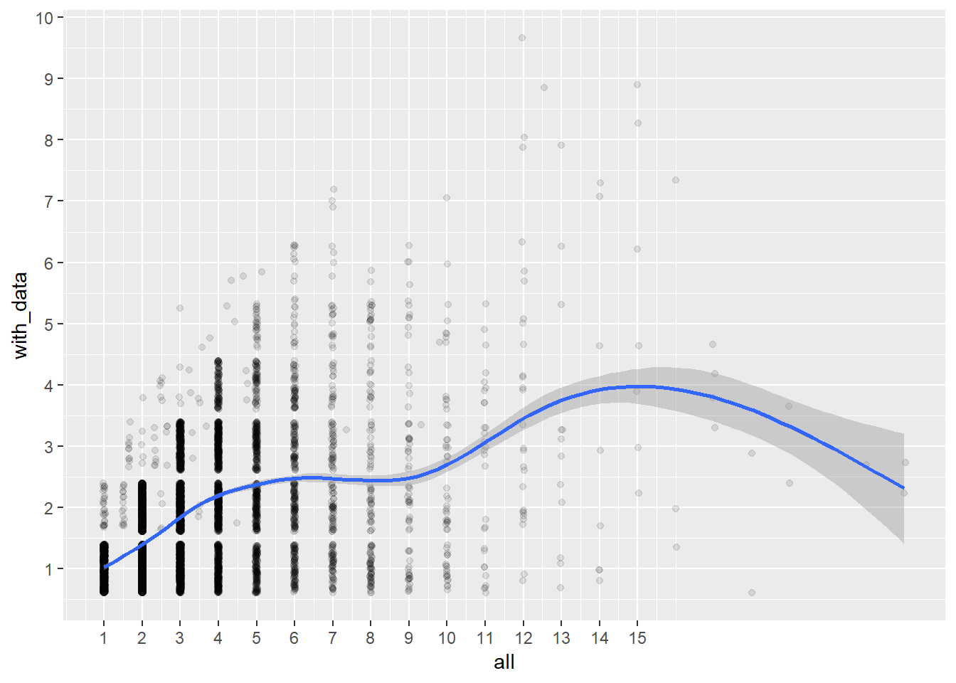

Maternal birthorder

descriptives = birthorder %>%
  group_by(group_outcome) %>%
  summarise(individuals = n(),
            mothers = length(unique(mother_pidlink)),
            sibship_size_mean = mean(sibling_count_uterus_alive, na.rm = T),
            sibship_size_confidence_low = mean(sibling_count_uterus_alive, na.rm = T) - 
              (qt(.975, n()-1)*sd(sibling_count_uterus_alive, na.rm = T)/sqrt(n())),
            sibship_size_confidence_high = mean(sibling_count_uterus_alive, na.rm = T) + 
              (qt(.975, n()-1)*sd(sibling_count_uterus_alive, na.rm = T)/sqrt(n())),
            sibship_size_min = min(sibling_count_uterus_alive, na.rm = TRUE),
            sibship_size_max = max(sibling_count_uterus_alive, na.rm = TRUE),
            birthorder_mean = mean(birthorder_uterus_alive, na.rm = T),
            birthorder_size_confidence_low = mean(birthorder_uterus_alive, na.rm = T) - 
              (qt(.975, n()-1)*sd(birthorder_uterus_alive, na.rm = T)/sqrt(n())),
            birthorder_size_confidence_high = mean(birthorder_uterus_alive, na.rm = T) + 
              (qt(.975, n()-1)*sd(birthorder_uterus_alive, na.rm = T)/sqrt(n())),
            birthorder_size_min = min(birthorder_uterus_alive, na.rm = TRUE),
            birthorder_size_max = max(birthorder_uterus_alive, na.rm = TRUE),
            number_siblings_mean = mean(sibling_count_uterus_alive, na.rm =T),
            number_siblings_confidence_low = mean(sibling_count_uterus_alive, na.rm = T) -
              (qt(.975, n()-1)*sd(sibling_count_uterus_alive, na.rm = T)/sqrt(n())),
            number_siblings_confidence_high = mean(sibling_count_uterus_alive, na.rm = T) +
              (qt(.975, n()-1)*sd(sibling_count_uterus_alive, na.rm = T)/sqrt(n())))

descriptives

group_outcome	individuals	mothers	sibship_size_mean	sibship_size_confidence_low	sibship_size_confidence_high	sibship_size_min	sibship_size_max	birthorder_mean	birthorder_size_confidence_low	birthorder_size_confidence_high	birthorder_size_min	birthorder_size_max	number_siblings_mean	number_siblings_confidence_low	number_siblings_confidence_high
control	55765	16301	4.614	4.587	4.641	1	22	2.775	2.757	2.793	1	22	4.614	4.587	4.641
test	45476	13187	3.823	3.8	3.845	1	22	2.454	2.436	2.471	1	21	3.823	3.8	3.845

birthorder %>% 
  t.test(sibling_count_uterus_alive ~ group_outcome, data = ., var.equal = T)

Two Sample t-test: `sibling_count_uterus_alive` by `group_outcome`
Test statistic	df	P value	Alternative hypothesis	mean in group control	mean in group test
26.37	43320	5.226e-152 * * *	two.sided	4.614	3.823

birthorder %>% 
  t.test(birthorder_uterus_alive ~ group_outcome, data = ., var.equal = T)

Two Sample t-test: `birthorder_uterus_alive` by `group_outcome`
Test statistic	df	P value	Alternative hypothesis	mean in group control	mean in group test
15.08	43320	2.809e-51 * * *	two.sided	2.775	2.454

How many siblings with data do we retain in each family?

birthorder %>% filter(!is.na(birthorder_uterus_alive), group_outcome == 1) %>% group_by(mother_pidlink) %>% summarise(with_data = n(), all = mean(sibling_count_uterus_alive)) -> counts
birthorder %>% filter(!is.na(birthorder_uterus_alive), group_outcome == 0) %>% group_by(mother_pidlink) %>% summarise(with_data = n(), all = mean(sibling_count_uterus_alive)) -> counts1

In our test sample families with an average size of NaN siblings, we retain 0.

In the original sample families with an average size of NaN siblings, we retain 0.

ggplot(counts, aes(all, with_data)) + geom_jitter(alpha = 0.1) + geom_smooth() + scale_x_continuous(breaks=1:15) + scale_y_continuous(breaks=1:15)

## `geom_smooth()` using method = 'loess' and formula 'y ~ x'

### Maternal pregnancy birthorder

descriptives = birthorder %>%
  group_by(group_outcome) %>%
  summarise(individuals = n(),
            mothers = length(unique(mother_pidlink)),
            sibship_size_mean = mean(sibling_count_uterus_preg, na.rm = T),
            sibship_size_confidence_low = mean(sibling_count_uterus_preg, na.rm = T) - 
              (qt(.975, n()-1)*sd(sibling_count_uterus_preg, na.rm = T)/sqrt(n())),
            sibship_size_confidence_high = mean(sibling_count_uterus_preg, na.rm = T) + 
              (qt(.975, n()-1)*sd(sibling_count_uterus_preg, na.rm = T)/sqrt(n())),
            sibship_size_min = min(sibling_count_uterus_preg, na.rm = TRUE),
            sibship_size_max = max(sibling_count_uterus_preg, na.rm = TRUE),
            birthorder_mean = mean(birthorder_uterus_preg, na.rm = T),
            birthorder_size_confidence_low = mean(birthorder_uterus_preg, na.rm = T) - 
              (qt(.975, n()-1)*sd(birthorder_uterus_preg, na.rm = T)/sqrt(n())),
            birthorder_size_confidence_high = mean(birthorder_uterus_preg, na.rm = T) + 
              (qt(.975, n()-1)*sd(birthorder_uterus_preg, na.rm = T)/sqrt(n())),
            birthorder_size_min = min(birthorder_uterus_preg, na.rm = TRUE),
            birthorder_size_max = max(birthorder_uterus_preg, na.rm = TRUE),
            number_siblings_mean = mean(sibling_count_uterus_preg, na.rm =T),
            number_siblings_confidence_low = mean(sibling_count_uterus_preg, na.rm = T) -
              (qt(.975, n()-1)*sd(sibling_count_uterus_preg, na.rm = T)/sqrt(n())),
            number_siblings_confidence_high = mean(sibling_count_uterus_preg, na.rm = T) +
              (qt(.975, n()-1)*sd(sibling_count_uterus_preg, na.rm = T)/sqrt(n())))

descriptives

group_outcome	individuals	mothers	sibship_size_mean	sibship_size_confidence_low	sibship_size_confidence_high	sibship_size_min	sibship_size_max	birthorder_mean	birthorder_size_confidence_low	birthorder_size_confidence_high	birthorder_size_min	birthorder_size_max	number_siblings_mean	number_siblings_confidence_low	number_siblings_confidence_high
control	55765	16301	5.184	5.154	5.214	1	26	3.072	3.052	3.093	1	26	5.184	5.154	5.214
test	45476	13187	4.279	4.253	4.305	1	26	2.663	2.644	2.683	1	25	4.279	4.253	4.305

birthorder %>% 
  t.test(sibling_count_uterus_preg ~ group_outcome, data = ., var.equal = T)

Two Sample t-test: `sibling_count_uterus_preg` by `group_outcome`
Test statistic	df	P value	Alternative hypothesis	mean in group control	mean in group test
27.27	48544	1.473e-162 * * *	two.sided	5.184	4.279

birthorder %>% 
  t.test(birthorder_uterus_preg ~ group_outcome, data = ., var.equal = T)

Two Sample t-test: `birthorder_uterus_preg` by `group_outcome`
Test statistic	df	P value	Alternative hypothesis	mean in group control	mean in group test
17.36	48544	2.76e-67 * * *	two.sided	3.072	2.663

How many siblings with data do we retain in each family?

birthorder %>% filter(!is.na(birthorder_uterus_preg), group_outcome == 1) %>% group_by(mother_pidlink) %>% summarise(with_data = n(), all = mean(sibling_count_uterus_preg)) -> counts
birthorder %>% filter(!is.na(birthorder_uterus_preg), group_outcome == 0) %>% group_by(mother_pidlink) %>% summarise(with_data = n(), all = mean(sibling_count_uterus_preg)) -> counts1

In our test sample families with an average size of NaN siblings, we retain 0.

In the original sample families with an average size of NaN siblings, we retain 0.

ggplot(counts, aes(all, with_data)) + geom_jitter(alpha = 0.1) + geom_smooth() + scale_x_continuous(breaks=1:15) + scale_y_continuous(breaks=1:15)

## `geom_smooth()` using method = 'loess' and formula 'y ~ x'

Outcome measurements and covariates

Control group

## Descriptives
descriptives = birthorder %>%
  group_by(group_birthorder) %>%
    summarise(n = n(),
              age_mean = mean(age, na.rm=TRUE),
              age_confidence_low = mean(age, na.rm = T) - 
                (qt(.975, n()-1)*sd(age, na.rm = T)/sqrt(n())),
              age_confidence_high = mean(age, na.rm = T) + 
                (qt(.975, n()-1)*sd(age, na.rm = T)/sqrt(n())),
              age_min = min(age, na.rm = TRUE),
              age_max = max(age, na.rm = TRUE),
              gender = mean(male, na.rm=TRUE))
descriptives

group_birthorder	n	age_mean	age_confidence_low	age_confidence_high	age_min	age_max	gender
control	58559	39.06	38.8	39.33	0	999	0.4885
test	42682	13.75	13.64	13.85	0	52	0.5104

## Ttest
tidy(t.test(birthorder$age ~ birthorder$group_birthorder, var.equal = T))

estimate1	estimate2	statistic	p.value	parameter	conf.low	conf.high	method	alternative
39.06	13.75	114.2	0	69280	24.89	25.75	Two Sample t-test	two.sided

cohen.d(birthorder$age, as.factor(birthorder$group_birthorder), na.rm = T)

## 
## Cohen's d
## 
## d estimate: 0.9244 (large)
## 95 percent confidence interval:
##  lower  upper 
## 0.9078 0.9410

gender = birthorder %>%
  group_by(group_birthorder) %>%
    summarise(gender = sum(male == 1, na.rm=T),
              gender2 = sum(male ==0,na.rm=T)) %>%
  select(gender, gender2)
prop.table(gender)

gender	gender2
0.3284	0.3438
0.1673	0.1605

tidy(chisq.test(gender))

statistic	p.value	parameter	method
29.15	0.0000000671	1	Pearson’s Chi-squared test with Yates’ continuity correction

## Ratings
ratings = birthorder %>%
  group_by(group_birthorder) %>%
  summarise(g_factor_mean = mean(g_factor_2015_old, na.rm=T),
            g_factor_confidence_low= mean(g_factor_2015_old, na.rm = T) - 
                (qt(.975, n()-1)*sd(g_factor_2015_old, na.rm = T)/sqrt(n())),
            g_factor_confidence_high = mean(g_factor_2015_old, na.rm = T) +
                (qt(.975, n()-1)*sd(g_factor_2015_old, na.rm = T)/sqrt(n())),
            big5_ext_mean = mean(big5_ext, na.rm=T),
            big5_ext_confidence_low= mean(big5_ext, na.rm = T) - 
                (qt(.975, n()-1)*sd(big5_ext, na.rm = T)/sqrt(n())),
            big5_ext_confidence_high = mean(big5_ext, na.rm = T) +
                (qt(.975, n()-1)*sd(big5_ext, na.rm = T)/sqrt(n())),
            big5_neu_mean = mean(big5_neu, na.rm=T),
            big5_neu_confidence_low= mean(big5_neu, na.rm = T) - 
                (qt(.975, n()-1)*sd(big5_neu, na.rm = T)/sqrt(n())),
            big5_neu_confidence_high = mean(big5_neu, na.rm = T) +
                (qt(.975, n()-1)*sd(big5_neu, na.rm = T)/sqrt(n())),
            big5_con_mean = mean(big5_con, na.rm=T),
            big5_con_confidence_low= mean(big5_con, na.rm = T) - 
                (qt(.975, n()-1)*sd(big5_con, na.rm = T)/sqrt(n())),
            big5_con_confidence_high = mean(big5_con, na.rm = T) +
                (qt(.975, n()-1)*sd(big5_con, na.rm = T)/sqrt(n())),
            big5_agree_mean = mean(big5_agree, na.rm=T),
            big5_agree_confidence_low= mean(big5_agree, na.rm = T) - 
                (qt(.975, n()-1)*sd(big5_agree, na.rm = T)/sqrt(n())),
            big5_agree_confidence_high = mean(big5_agree, na.rm = T) +
                (qt(.975, n()-1)*sd(big5_agree, na.rm = T)/sqrt(n())),
            big5_open_mean = mean(big5_open, na.rm=T),
            big5_open_confidence_low= mean(big5_open, na.rm = T) - 
                (qt(.975, n()-1)*sd(big5_open, na.rm = T)/sqrt(n())),
            big5_open_confidence_high = mean(big5_open, na.rm = T) +
                (qt(.975, n()-1)*sd(big5_open, na.rm = T)/sqrt(n())),
            riskA_mean = mean(riskA, na.rm=T),
            riskA_confidence_low= mean(riskA, na.rm = T) - 
                (qt(.975, n()-1)*sd(riskA, na.rm = T)/sqrt(n())),
            riskA_confidence_high = mean(riskA, na.rm = T) +
                (qt(.975, n()-1)*sd(riskA, na.rm = T)/sqrt(n())),
            riskB_mean = mean(riskB, na.rm=T),
            riskB_confidence_low= mean(riskB, na.rm = T) - 
                (qt(.975, n()-1)*sd(riskB, na.rm = T)/sqrt(n())),
            riskB_confidence_high = mean(riskB, na.rm = T) +
                (qt(.975, n()-1)*sd(riskB, na.rm = T)/sqrt(n())))
ratings

group_birthorder	g_factor_mean	g_factor_confidence_low	g_factor_confidence_high	big5_ext_mean	big5_ext_confidence_low	big5_ext_confidence_high	big5_neu_mean	big5_neu_confidence_low	big5_neu_confidence_high	big5_con_mean	big5_con_confidence_low	big5_con_confidence_high	big5_agree_mean	big5_agree_confidence_low	big5_agree_confidence_high	big5_open_mean	big5_open_confidence_low	big5_open_confidence_high	riskA_mean	riskA_confidence_low	riskA_confidence_high	riskB_mean	riskB_confidence_low	riskB_confidence_high
control	-0.1381	-0.1448	-0.1314	3.429	3.424	3.434	2.669	2.664	2.674	3.837	3.833	3.842	3.915	3.911	3.919	3.674	3.668	3.68	3.433	3.421	3.446	4.185	4.174	4.197
test	0.4502	0.4438	0.4567	3.493	3.487	3.5	2.724	2.717	2.73	3.73	3.724	3.735	3.85	3.846	3.855	3.817	3.812	3.823	3.292	3.278	3.305	4.288	4.276	4.301

tidy(t.test(birthorder$g_factor_2015_old ~ birthorder$group_birthorder, var.equal = T))

estimate1	estimate2	statistic	p.value	parameter	conf.low	conf.high	method	alternative
-0.1381	0.4502	-51.98	0	27524	-0.6105	-0.5661	Two Sample t-test	two.sided

cohen.d(birthorder$g_factor_2015_old, as.factor(birthorder$group_birthorder), na.rm = T)

## 
## Cohen's d
## 
## d estimate: -0.7392 (medium)
## 95 percent confidence interval:
##   lower   upper 
## -0.7678 -0.7107

tidy(t.test(birthorder$years_of_education ~ birthorder$group_birthorder, var.equal = T))

estimate1	estimate2	statistic	p.value	parameter	conf.low	conf.high	method	alternative
8.283	11.4	-49.98	0	33816	-3.236	-2.992	Two Sample t-test	two.sided

cohen.d(birthorder$years_of_education, as.factor(birthorder$group_birthorder), na.rm = T)

## 
## Cohen's d
## 
## d estimate: -0.6763 (medium)
## 95 percent confidence interval:
##   lower   upper 
## -0.7033 -0.6493

tidy(t.test(birthorder$big5_ext ~ birthorder$group_birthorder, var.equal = T))

estimate1	estimate2	statistic	p.value	parameter	conf.low	conf.high	method	alternative
3.429	3.493	-6.982	2.971e-12	31444	-0.08258	-0.04638	Two Sample t-test	two.sided

cohen.d(birthorder$big5_ext, as.factor(birthorder$group_birthorder), na.rm = T)

## 
## Cohen's d
## 
## d estimate: -0.09677 (negligible)
## 95 percent confidence interval:
##    lower    upper 
## -0.12395 -0.06959

tidy(t.test(birthorder$big5_neu ~ birthorder$group_birthorder, var.equal = T))

estimate1	estimate2	statistic	p.value	parameter	conf.low	conf.high	method	alternative
2.669	2.724	-5.923	0.000000003185	31444	-0.07268	-0.03654	Two Sample t-test	two.sided

cohen.d(birthorder$big5_neu, as.factor(birthorder$group_birthorder), na.rm = T)

## 
## Cohen's d
## 
## d estimate: -0.0821 (negligible)
## 95 percent confidence interval:
##    lower    upper 
## -0.10927 -0.05493

tidy(t.test(birthorder$big5_con ~ birthorder$group_birthorder, var.equal = T))

estimate1	estimate2	statistic	p.value	parameter	conf.low	conf.high	method	alternative
3.837	3.73	14.06	9.458e-45	31444	0.09249	0.1225	Two Sample t-test	two.sided

cohen.d(birthorder$big5_con, as.factor(birthorder$group_birthorder), na.rm = T)

## 
## Cohen's d
## 
## d estimate: 0.1948 (negligible)
## 95 percent confidence interval:
##  lower  upper 
## 0.1676 0.2221

tidy(t.test(birthorder$big5_agree ~ birthorder$group_birthorder, var.equal = T))

estimate1	estimate2	statistic	p.value	parameter	conf.low	conf.high	method	alternative
3.915	3.85	9.136	6.863e-20	31444	0.0508	0.07854	Two Sample t-test	two.sided

cohen.d(birthorder$big5_agree, as.factor(birthorder$group_birthorder), na.rm = T)

## 
## Cohen's d
## 
## d estimate: 0.1266 (negligible)
## 95 percent confidence interval:
##   lower   upper 
## 0.09944 0.15381

tidy(t.test(birthorder$big5_open ~ birthorder$group_birthorder, var.equal = T))

estimate1	estimate2	statistic	p.value	parameter	conf.low	conf.high	method	alternative
3.674	3.817	-15.52	3.76e-54	31444	-0.1615	-0.1253	Two Sample t-test	two.sided

cohen.d(birthorder$big5_open, as.factor(birthorder$group_birthorder), na.rm = T)

## 
## Cohen's d
## 
## d estimate: -0.2152 (small)
## 95 percent confidence interval:
##   lower   upper 
## -0.2424 -0.1880

tidy(t.test(birthorder$riskA ~ birthorder$group_birthorder, var.equal = T))

estimate1	estimate2	statistic	p.value	parameter	conf.low	conf.high	method	alternative
3.433	3.292	6.415	0.0000000001434	27778	0.0985	0.1852	Two Sample t-test	two.sided

cohen.d(birthorder$riskA, as.factor(birthorder$group_birthorder), na.rm = T)

## 
## Cohen's d
## 
## d estimate: 0.094 (negligible)
## 95 percent confidence interval:
##   lower   upper 
## 0.06526 0.12273

tidy(t.test(birthorder$riskB ~ birthorder$group_birthorder, var.equal = T))

estimate1	estimate2	statistic	p.value	parameter	conf.low	conf.high	method	alternative
4.185	4.288	-5.116	0.0000003147	29576	-0.1426	-0.06362	Two Sample t-test	two.sided

cohen.d(birthorder$riskB, as.factor(birthorder$group_birthorder), na.rm = T)

## 
## Cohen's d
## 
## d estimate: -0.0729 (negligible)
## 95 percent confidence interval:
##    lower    upper 
## -0.10084 -0.04496

## Educational Attainment
educational_attainment = birthorder %>%
  group_by(group_birthorder) %>%
  summarise(years_of_education_mean = mean(years_of_education, na.rm=T),
            years_of_education_confidence_low= mean(years_of_education, na.rm = T) - 
                (qt(.975, n()-1)*sd(years_of_education, na.rm = T)/sqrt(n())),
            years_of_education_high = mean(years_of_education, na.rm = T) +
                (qt(.975, n()-1)*sd(years_of_education, na.rm = T)/sqrt(n())))

educational_attainment

group_birthorder	years_of_education_mean	years_of_education_confidence_low	years_of_education_high
control	8.283	8.244	8.322
test	11.4	11.36	11.43

t.test(birthorder$years_of_education ~ birthorder$group_birthorder, var.equal = T)

Two Sample t-test: `birthorder$years_of_education` by `birthorder$group_birthorder`
Test statistic	df	P value	Alternative hypothesis	mean in group control	mean in group test
-49.98	33816	0 * * *	two.sided	8.283	11.4

ggplot(data=birthorder, aes(x=years_of_education, fill=group_birthorder)) +
  geom_histogram(stat="count", binwidth=.5, position="dodge")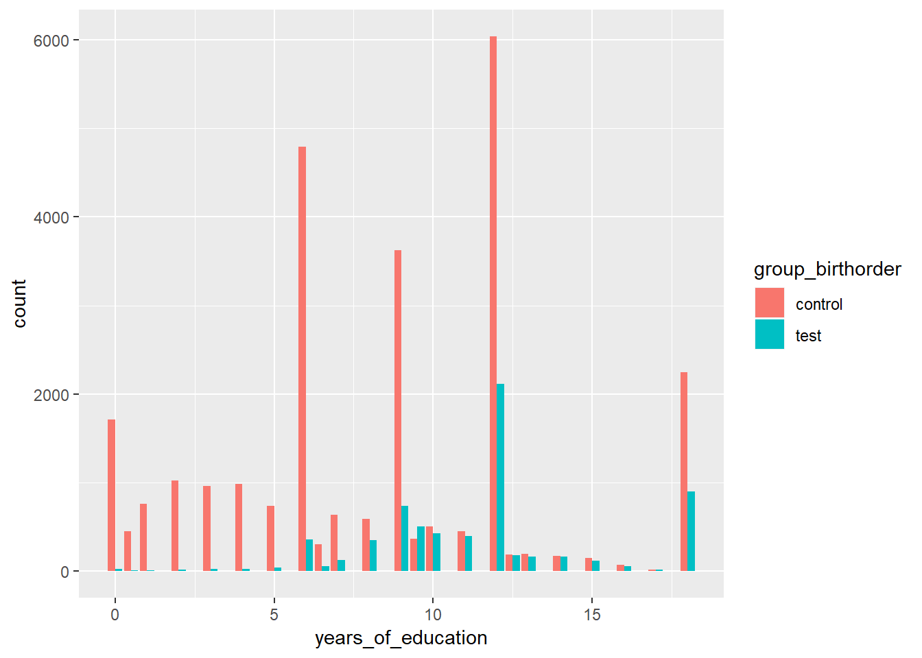

Descriptives

x = birthorder %>% filter(group_birthorder == "test", group_outcome == "test")
mean_sd = birthorder %>%
  group_by(group_birthorder) %>%
  summarise(age_mean = mean(age, na.rm=T),
            age_sd = sd(age, na.rm=T),
            g_factor_mean = mean(g_factor_2015_old, na.rm=T),
            g_factor_sd = sd(g_factor_2015_old, na.rm=T),
            big5_ext_mean = mean(big5_ext, na.rm=T),
            big5_ext_sd = sd(big5_ext, na.rm=T),
            big5_neu_mean = mean(big5_neu, na.rm=T),
            big5_neu_sd = sd(big5_neu, na.rm=T),
            big5_con_mean = mean(big5_con, na.rm=T),
            big5_con_sd = sd(big5_con, na.rm=T),
            big5_agree_mean = mean(big5_agree, na.rm=T),
            big5_agree_sd = sd(big5_agree, na.rm=T),
            big5_open_mean = mean(big5_open, na.rm=T),
            big5_open_sd = sd(big5_open, na.rm=T),
            riskA_mean = mean(riskA, na.rm=T),
            riskA_sd = sd(riskA, na.rm=T),
            riskB_mean = mean(riskB, na.rm=T),
            riskB_sd = sd(riskB, na.rm=T),
            years_of_education_mean = mean(years_of_education, na.rm=T),
            years_of_education_sd = sd(years_of_education, na.rm=T))
      
mean_sd

group_birthorder	age_mean	age_sd	g_factor_mean	g_factor_sd	big5_ext_mean	big5_ext_sd	big5_neu_mean	big5_neu_sd	big5_con_mean	big5_con_sd	big5_agree_mean	big5_agree_sd	big5_open_mean	big5_open_sd	riskA_mean	riskA_sd	riskB_mean	riskB_sd	years_of_education_mean	years_of_education_sd
control	39.06	32.54	-0.1381	0.8272	3.429	0.6616	2.669	0.6655	3.837	0.5447	3.915	0.5111	3.674	0.6824	3.433	1.528	4.185	1.441	8.283	4.847
test	13.75	10.83	0.4502	0.6835	3.493	0.6839	2.724	0.6638	3.73	0.5768	3.85	0.5094	3.817	0.6013	3.292	1.437	4.288	1.313	11.4	3.488

Correlations

cor = round(cor(birthorder %>% filter(group_birthorder == "test", group_outcome == "test") %>% ungroup() %>% select(age, male, g_factor_2015_old, years_of_education, big5_ext, big5_neu, big5_con, big5_agree, big5_open, riskA, riskB), use = "pairwise.complete.obs"), 2) 

cor

age	male	g_factor_2015_old	years_of_education	big5_ext	big5_neu	big5_con	big5_agree	big5_open	riskA	riskB
1	-0.03	-0.1	0.24	0	-0.13	0.24	0.1	0	-0.06	-0.01
-0.03	1	-0.01	-0.05	-0.13	-0.13	0.02	0.03	0.08	-0.13	-0.12
-0.1	-0.01	1	0.35	0.06	-0.05	-0.03	-0.04	0.08	-0.15	0.05
0.24	-0.05	0.35	1	0.07	-0.08	0.1	0.03	0.15	-0.19	-0.02
0	-0.13	0.06	0.07	1	-0.09	0.07	0.07	0.17	-0.01	0
-0.13	-0.13	-0.05	-0.08	-0.09	1	-0.2	-0.17	-0.07	0.04	0.02
0.24	0.02	-0.03	0.1	0.07	-0.2	1	0.32	0.27	-0.04	0.02
0.1	0.03	-0.04	0.03	0.07	-0.17	0.32	1	0.23	-0.02	-0.01
0	0.08	0.08	0.15	0.17	-0.07	0.27	0.23	1	-0.08	-0.03
-0.06	-0.13	-0.15	-0.19	-0.01	0.04	-0.04	-0.02	-0.08	1	0.3
-0.01	-0.12	0.05	-0.02	0	0.02	0.02	-0.01	-0.03	0.3	1

Reliability

Intelligence

alpha(birthorder %>% filter(group_birthorder == "test", group_outcome == "test") %>% ungroup() %>% select(raven_2015_old, math_2015_old, count_backwards, words_delayed, adaptive_numbering))

## 
## Reliability analysis   
## Call: alpha(x = birthorder %>% filter(group_birthorder == "test", group_outcome == 
##     "test") %>% ungroup() %>% select(raven_2015_old, math_2015_old, 
##     count_backwards, words_delayed, adaptive_numbering))
## 
##   raw_alpha std.alpha G6(smc) average_r S/N     ase mean sd median_r
##      0.025      0.61    0.56      0.24 1.6 0.00066  109 16     0.22
## 
##  lower alpha upper     95% confidence boundaries
## 0.02 0.03 0.03 
## 
##  Reliability if an item is dropped:
##                    raw_alpha std.alpha G6(smc) average_r S/N alpha se  var.r med.r
## raven_2015_old         0.024      0.54    0.47      0.23 1.2  0.00069 0.0026  0.22
## math_2015_old          0.022      0.53    0.46      0.22 1.1  0.00068 0.0029  0.19
## count_backwards        0.023      0.57    0.51      0.25 1.4  0.00069 0.0042  0.25
## words_delayed          0.011      0.60    0.53      0.27 1.5  0.00020 0.0027  0.29
## adaptive_numbering     0.214      0.53    0.46      0.22 1.1  0.00484 0.0040  0.20
## 
##  Item statistics 
##                       n raw.r std.r r.cor r.drop   mean    sd
## raven_2015_old     6598  0.27  0.64  0.50   0.30   0.75  0.21
## math_2015_old      6598  0.26  0.66  0.54   0.30   0.44  0.30
## count_backwards    6492  0.26  0.60  0.42   0.28   0.80  0.26
## words_delayed      6593  0.20  0.56  0.35   0.20   5.04  1.68
## adaptive_numbering 6581  0.88  0.66  0.53   0.29 539.96 54.83

Personality

##Extraversion
alpha(birthorder %>% filter(group_birthorder == "test", group_outcome == "test") %>% ungroup() %>%
        select(e1, e2r_reversed, e3))

## 
## Reliability analysis   
## Call: alpha(x = birthorder %>% filter(group_birthorder == "test", group_outcome == 
##     "test") %>% ungroup() %>% select(e1, e2r_reversed, e3))
## 
##   raw_alpha std.alpha G6(smc) average_r  S/N    ase mean   sd median_r
##       0.45      0.43    0.35       0.2 0.77 0.0072  3.5 0.68     0.17
## 
##  lower alpha upper     95% confidence boundaries
## 0.43 0.45 0.46 
## 
##  Reliability if an item is dropped:
##              raw_alpha std.alpha G6(smc) average_r  S/N alpha se var.r med.r
## e1                0.17      0.19    0.11      0.11 0.24   0.0121    NA  0.11
## e2r_reversed      0.26      0.29    0.17      0.17 0.42   0.0106    NA  0.17
## e3                0.50      0.50    0.33      0.33 1.00   0.0083    NA  0.33
## 
##  Item statistics 
##                 n raw.r std.r r.cor r.drop mean   sd
## e1           6584  0.79  0.73  0.52   0.36  3.2 1.13
## e2r_reversed 6584  0.76  0.70  0.45   0.32  3.0 1.11
## e3           6584  0.48  0.62  0.25   0.17  4.2 0.67
## 
## Non missing response frequency for each item
##                 1    2    3    4    5 miss
## e1           0.02 0.35 0.11 0.40 0.12 0.55
## e2r_reversed 0.07 0.34 0.11 0.43 0.05 0.55
## e3           0.00 0.02 0.06 0.61 0.30 0.55

## Neuroticism
alpha(birthorder %>% filter(group_birthorder == "test", group_outcome == "test") %>% ungroup()
      %>% select(n1r_reversed, n2, n3))

## 
## Reliability analysis   
## Call: alpha(x = birthorder %>% filter(group_birthorder == "test", group_outcome == 
##     "test") %>% ungroup() %>% select(n1r_reversed, n2, n3))
## 
##   raw_alpha std.alpha G6(smc) average_r S/N    ase mean   sd median_r
##       0.37      0.33    0.29      0.14 0.5 0.0084  2.7 0.66    0.056
## 
##  lower alpha upper     95% confidence boundaries
## 0.35 0.37 0.38 
## 
##  Reliability if an item is dropped:
##              raw_alpha std.alpha G6(smc) average_r   S/N alpha se var.r med.r
## n1r_reversed     0.510     0.510   0.342     0.342 1.041   0.0081    NA 0.342
## n2               0.099     0.105   0.056     0.056 0.118   0.0140    NA 0.056
## n3               0.059     0.062   0.032     0.032 0.067   0.0145    NA 0.032
## 
##  Item statistics 
##                 n raw.r std.r r.cor r.drop mean   sd
## n1r_reversed 6584  0.43  0.55 0.087  0.053  2.1 0.77
## n2           6584  0.75  0.70 0.469  0.291  3.1 1.11
## n3           6584  0.76  0.71 0.493  0.308  3.0 1.09
## 
## Non missing response frequency for each item
##                 1    2    3    4    5 miss
## n1r_reversed 0.17 0.67 0.08 0.07 0.01 0.55
## n2           0.02 0.39 0.10 0.40 0.09 0.55
## n3           0.03 0.46 0.09 0.36 0.06 0.55

##conscientiousness
alpha(birthorder %>% filter(group_birthorder == "test", group_outcome == "test") %>% ungroup() %>% select(c1, c2r_reversed, c3))

## 
## Reliability analysis   
## Call: alpha(x = birthorder %>% filter(group_birthorder == "test", group_outcome == 
##     "test") %>% ungroup() %>% select(c1, c2r_reversed, c3))
## 
##   raw_alpha std.alpha G6(smc) average_r  S/N   ase mean   sd median_r
##       0.37      0.39    0.31      0.18 0.65 0.009  3.7 0.58     0.19
## 
##  lower alpha upper     95% confidence boundaries
## 0.36 0.37 0.39 
## 
##  Reliability if an item is dropped:
##              raw_alpha std.alpha G6(smc) average_r  S/N alpha se var.r med.r
## c1                0.17      0.17   0.094     0.094 0.21   0.0135    NA 0.094
## c2r_reversed      0.39      0.40   0.249     0.249 0.66   0.0098    NA 0.249
## c3                0.31      0.32   0.189     0.189 0.47   0.0109    NA 0.189
## 
##  Item statistics 
##                 n raw.r std.r r.cor r.drop mean   sd
## c1           6584  0.65  0.71  0.47   0.29  4.1 0.73
## c2r_reversed 6584  0.70  0.64  0.29   0.17  3.4 0.99
## c3           6584  0.65  0.67  0.36   0.21  3.8 0.86
## 
## Non missing response frequency for each item
##                 1    2    3    4    5 miss
## c1           0.00 0.04 0.07 0.63 0.25 0.55
## c2r_reversed 0.03 0.25 0.11 0.56 0.05 0.55
## c3           0.01 0.11 0.12 0.63 0.13 0.55

##Agreeableness
alpha(birthorder %>% filter(group_birthorder == "test", group_outcome == "test") %>% ungroup() %>% select(a1, a2, a3r_reversed))

## 
## Reliability analysis   
## Call: alpha(x = birthorder %>% filter(group_birthorder == "test", group_outcome == 
##     "test") %>% ungroup() %>% select(a1, a2, a3r_reversed))
## 
##   raw_alpha std.alpha G6(smc) average_r  S/N  ase mean   sd median_r
##       0.28      0.36    0.33      0.16 0.57 0.01  3.9 0.51    0.047
## 
##  lower alpha upper     95% confidence boundaries
## 0.26 0.28 0.3 
## 
##  Reliability if an item is dropped:
##              raw_alpha std.alpha G6(smc) average_r   S/N alpha se var.r med.r
## a1               0.048     0.054   0.028     0.028 0.057    0.014    NA 0.028
## a2               0.081     0.089   0.047     0.047 0.098    0.014    NA 0.047
## a3r_reversed     0.577     0.577   0.406     0.406 1.367    0.007    NA 0.406
## 
##  Item statistics 
##                 n raw.r std.r r.cor r.drop mean   sd
## a1           6584  0.63  0.73 0.544  0.250  4.2 0.66
## a2           6584  0.61  0.72 0.526  0.236  4.1 0.64
## a3r_reversed 6584  0.71  0.54 0.067  0.044  3.2 1.03
## 
## Non missing response frequency for each item
##                 1    2    3    4    5 miss
## a1           0.00 0.02 0.06 0.62 0.30 0.55
## a2           0.00 0.02 0.08 0.66 0.24 0.55
## a3r_reversed 0.03 0.29 0.12 0.51 0.05 0.55

##Openness
alpha(birthorder %>% filter(group_birthorder == "test", group_outcome == "test") %>% ungroup() %>% select(o1, o2, o3))

## 
## Reliability analysis   
## Call: alpha(x = birthorder %>% filter(group_birthorder == "test", group_outcome == 
##     "test") %>% ungroup() %>% select(o1, o2, o3))
## 
##   raw_alpha std.alpha G6(smc) average_r  S/N    ase mean  sd median_r
##       0.46      0.46    0.37      0.22 0.86 0.0077  3.8 0.6     0.22
## 
##  lower alpha upper     95% confidence boundaries
## 0.44 0.46 0.47 
## 
##  Reliability if an item is dropped:
##    raw_alpha std.alpha G6(smc) average_r  S/N alpha se var.r med.r
## o1      0.32      0.33    0.20      0.20 0.49   0.0109    NA  0.20
## o2      0.40      0.40    0.25      0.25 0.67   0.0098    NA  0.25
## o3      0.36      0.36    0.22      0.22 0.57   0.0104    NA  0.22
## 
##  Item statistics 
##       n raw.r std.r r.cor r.drop mean   sd
## o1 6584  0.71  0.71  0.45   0.30  3.8 0.87
## o2 6584  0.72  0.68  0.39   0.27  3.6 0.96
## o3 6584  0.65  0.69  0.42   0.28  4.1 0.76
## 
## Non missing response frequency for each item
##       1    2    3    4    5 miss
## o1 0.01 0.12 0.11 0.62 0.14 0.55
## o2 0.02 0.17 0.13 0.56 0.13 0.55
## o3 0.01 0.05 0.07 0.61 0.27 0.55

Plots age and gender

Plots Gender

birthorder = birthorder %>% filter(age<=100)

birthorder = birthorder %>%
  mutate(outcome = age)
plot_gender(birthorder)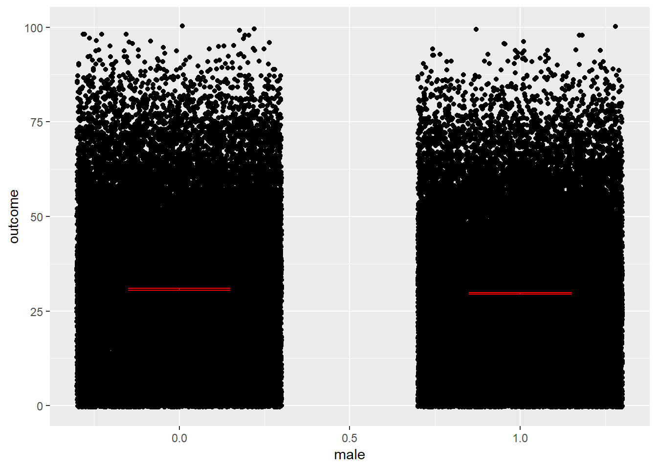

birthorder = birthorder %>%
  mutate(outcome = birthorder_genes)
plot_gender(birthorder)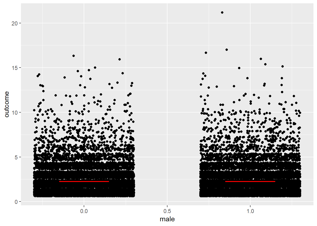

birthorder = birthorder %>%
  mutate(outcome = sibling_count_genes)
plot_gender(birthorder)

birthorder = birthorder %>%
  mutate(outcome = g_factor_2015_old)
plot_gender(birthorder)

birthorder = birthorder %>%
  mutate(outcome = g_factor_2015_young)
plot_gender(birthorder)

birthorder = birthorder %>%
  mutate(outcome = g_factor_2007_old)
plot_gender(birthorder)

birthorder = birthorder %>%
  mutate(outcome = g_factor_2007_young)
plot_gender(birthorder)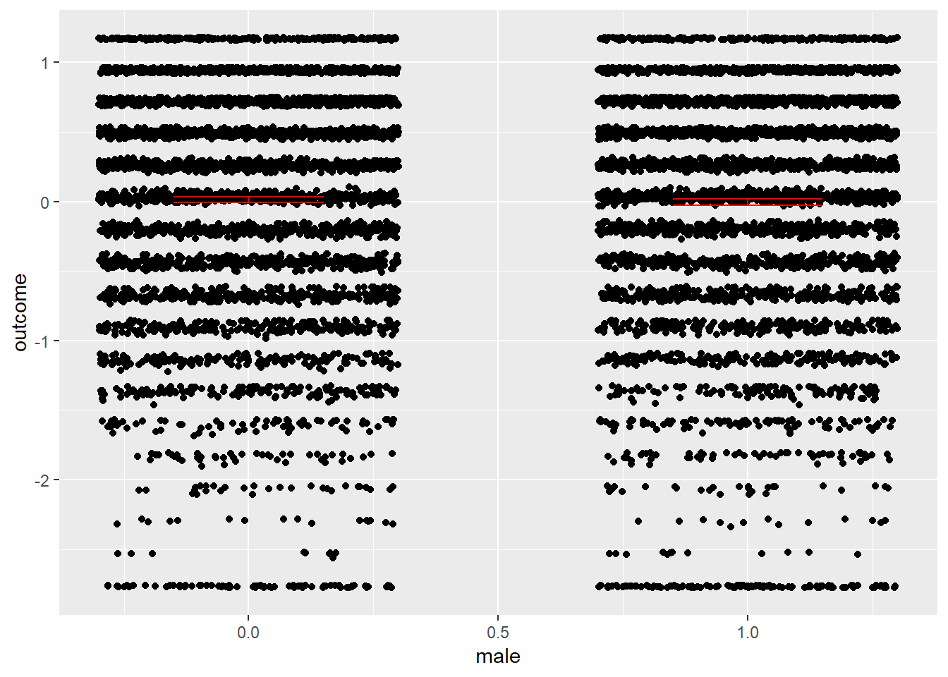

birthorder = birthorder %>%
  mutate(outcome = big5_ext)
plot_gender(birthorder)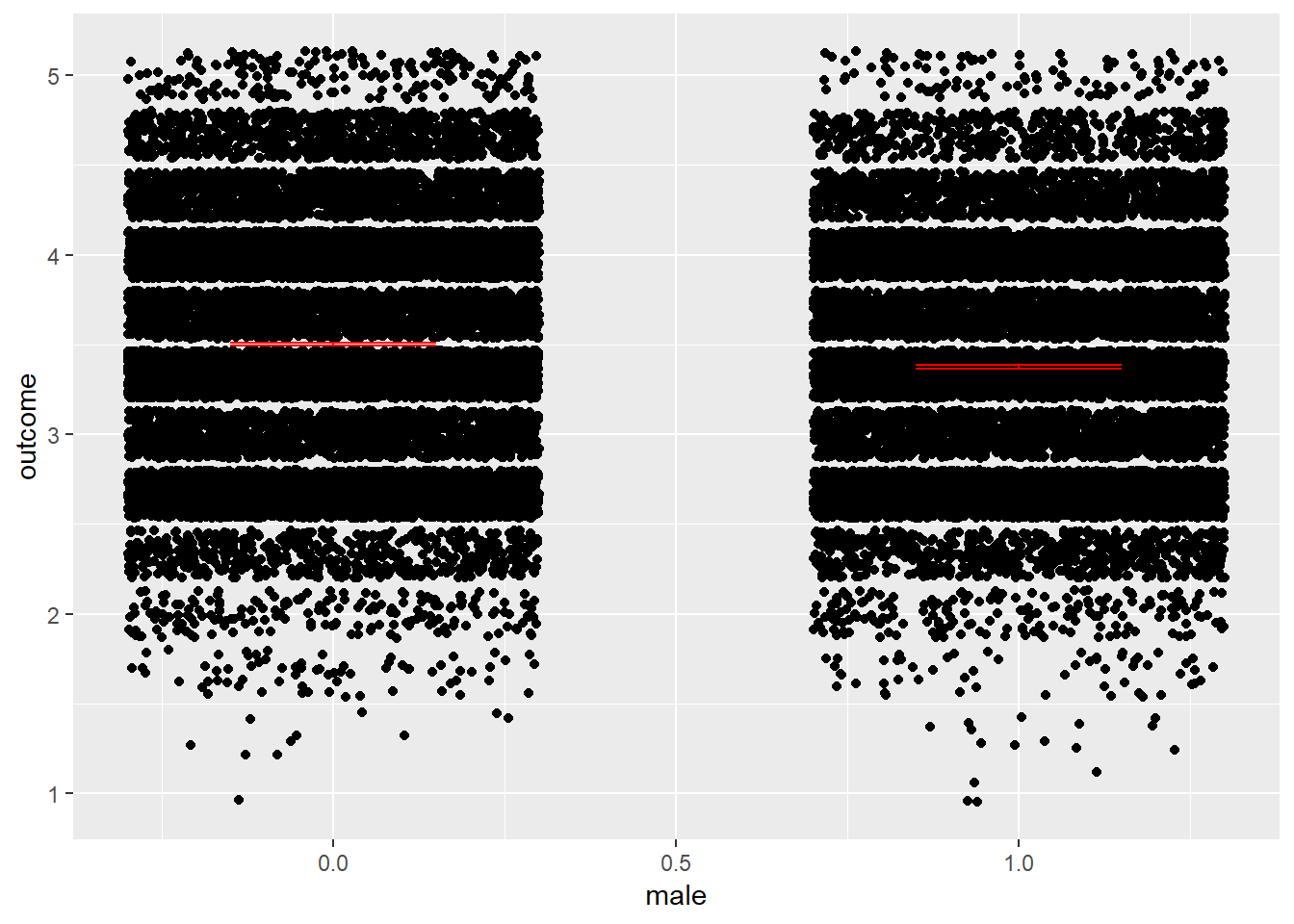

birthorder = birthorder %>%
  mutate(outcome = big5_con)
plot_gender(birthorder)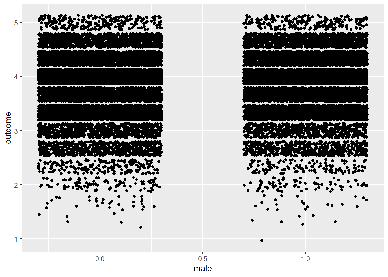

birthorder = birthorder %>%
  mutate(outcome = big5_open)
plot_gender(birthorder)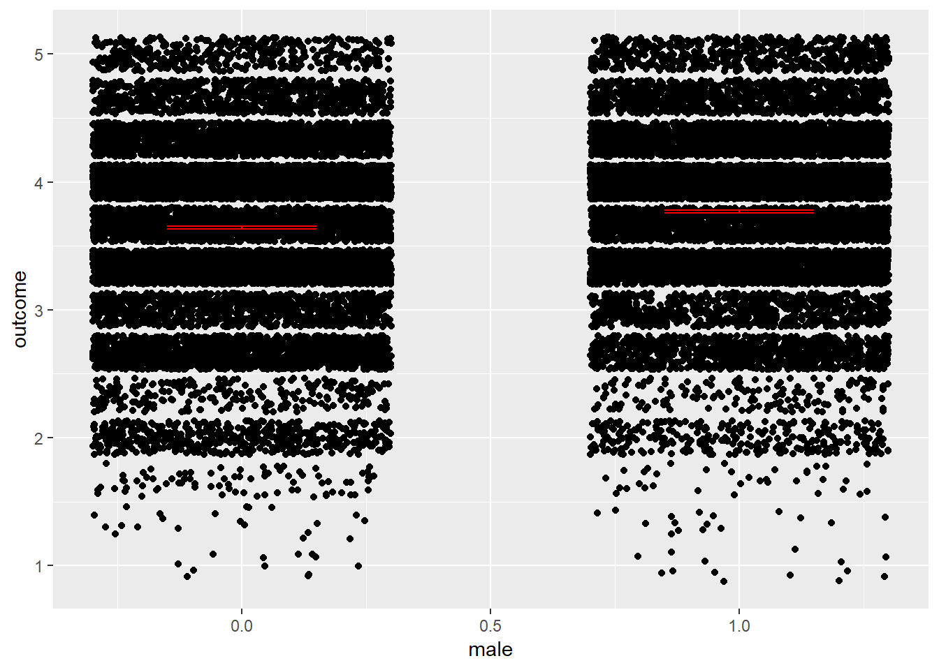

birthorder = birthorder %>%
  mutate(outcome = big5_neu)
plot_gender(birthorder)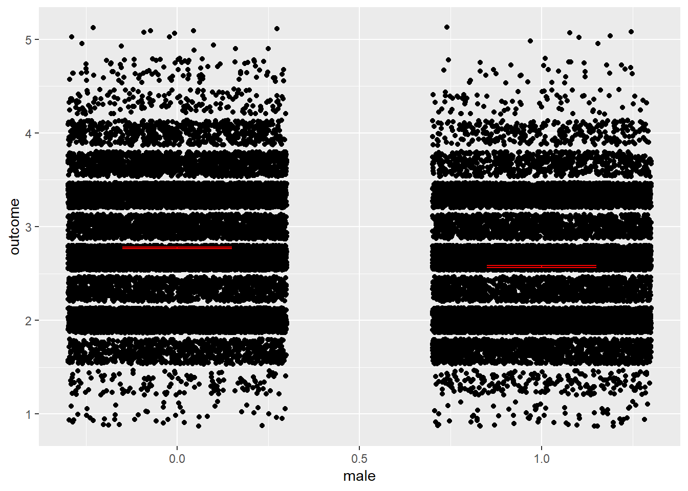

birthorder = birthorder %>%
  mutate(outcome = big5_agree)
plot_gender(birthorder)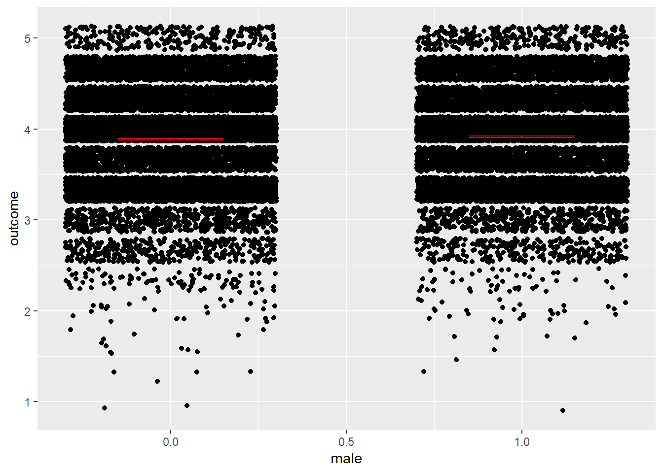

birthorder = birthorder %>%
  mutate(outcome = riskA)
plot_gender(birthorder)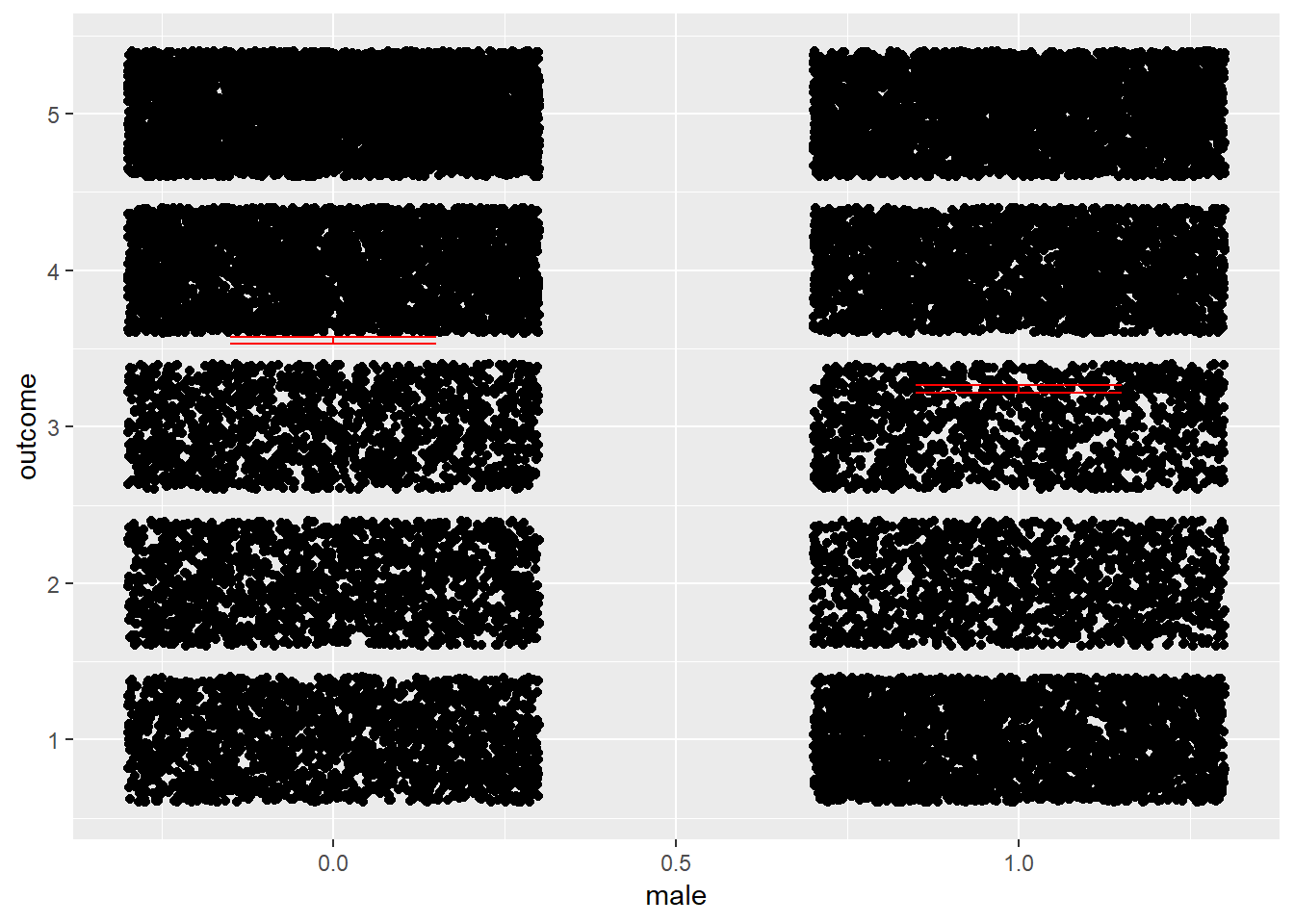

birthorder = birthorder %>%
  mutate(outcome = riskB)
plot_gender(birthorder)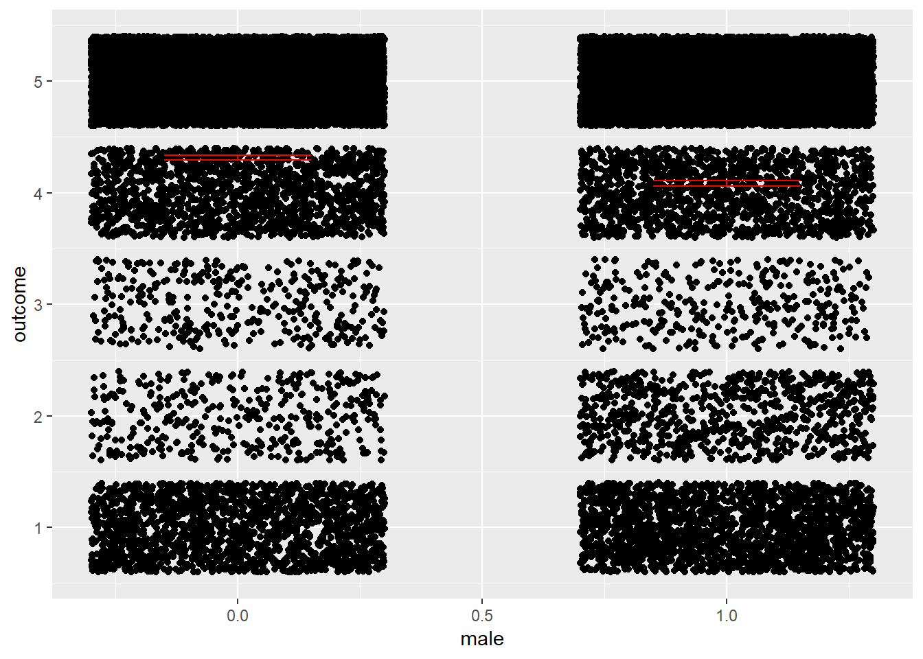

birthorder = birthorder %>%
  mutate(outcome = years_of_education)
plot_gender(birthorder)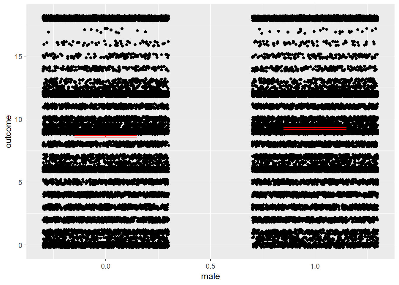

plot_gender(birthorder %>% filter(!is.na(attended_school)) %>% mutate(outcome = as.numeric(attended_school)))

birthorder = birthorder %>%
  mutate(outcome = Elementary_missed)
plot_gender(birthorder)

birthorder = birthorder %>%
  mutate(outcome = Elementary_worked)
plot_gender(birthorder)

birthorder = birthorder %>%
  mutate(outcome = wage_last_month_log)
plot_gender(birthorder)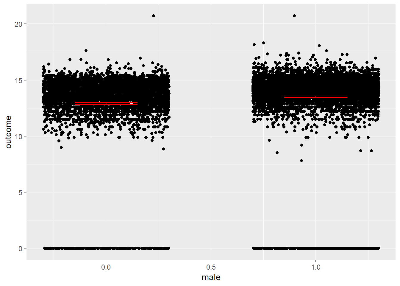

birthorder = birthorder %>%
  mutate(outcome = wage_last_year_log)
plot_gender(birthorder)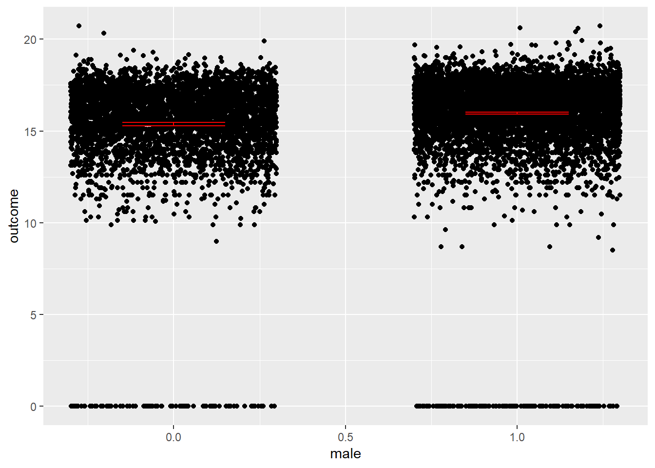

birthorder = birthorder %>%
  mutate(outcome = Self_employed)
plot_gender(birthorder)

birthorder = birthorder %>%
  mutate(outcome = ever_smoked)
plot_gender(birthorder)

Plots Age

plot_age(birthorder %>% filter(age<= 100) %>% mutate(outcome = birthorder_genes))

## `geom_smooth()` using method = 'gam' and formula 'y ~ s(x, bs = "cs")'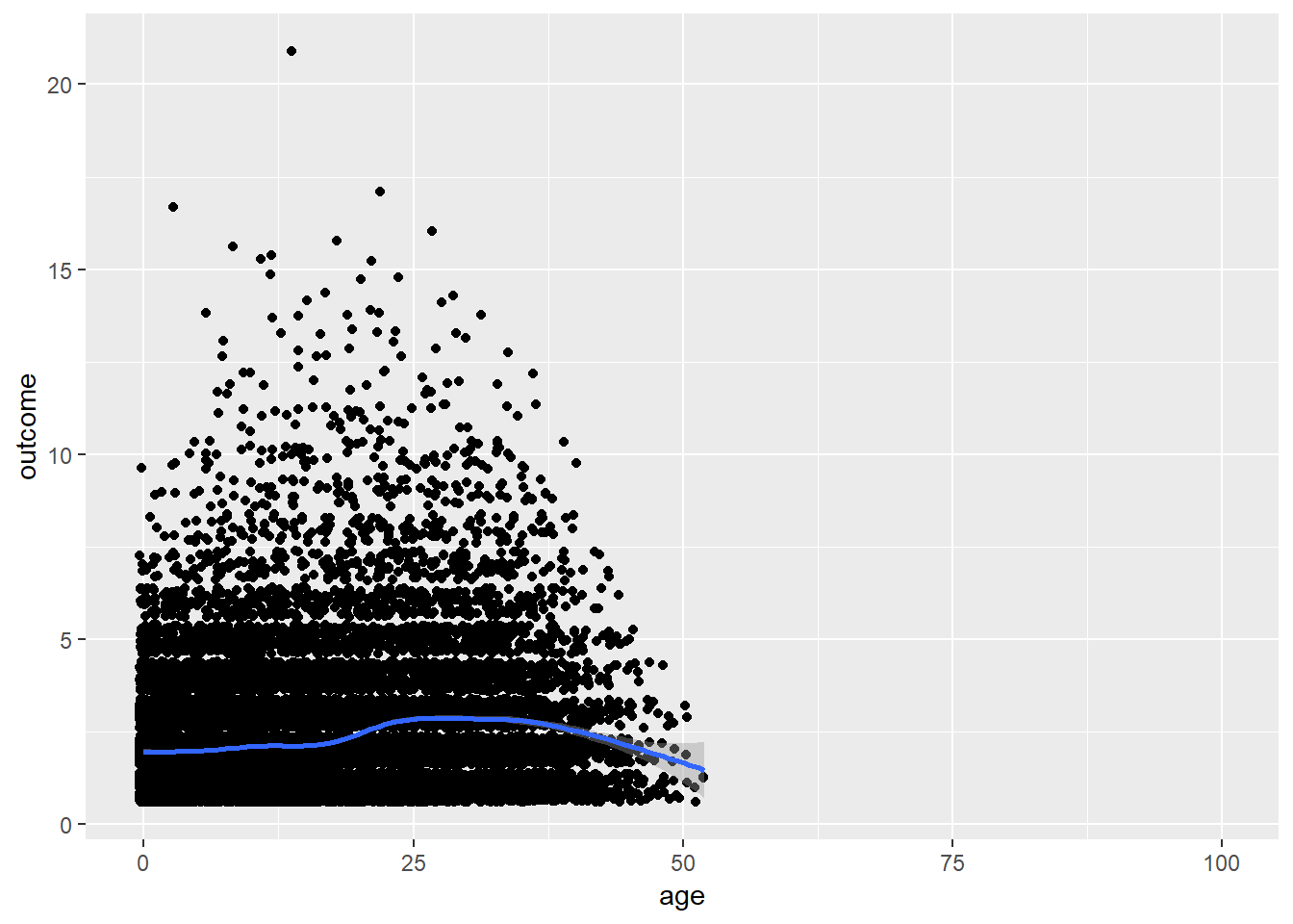

birthorder = birthorder %>%
  mutate(outcome = sibling_count_genes)
plot_age(birthorder)

## `geom_smooth()` using method = 'gam' and formula 'y ~ s(x, bs = "cs")'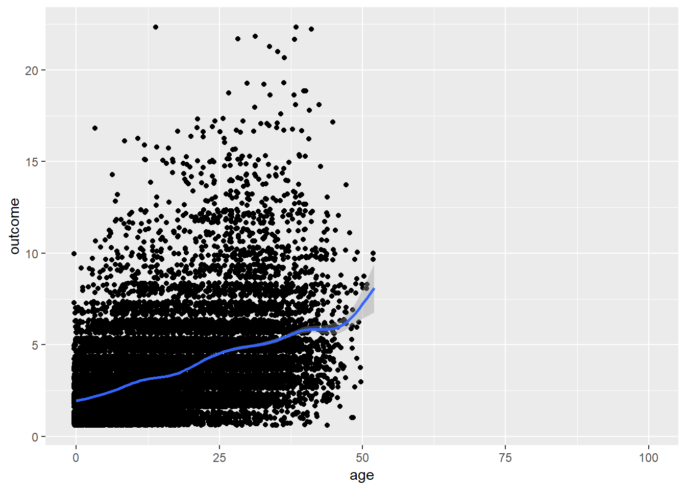

birthorder = birthorder %>%
  mutate(outcome = g_factor_2015_old)
plot_age(birthorder)

## `geom_smooth()` using method = 'gam' and formula 'y ~ s(x, bs = "cs")'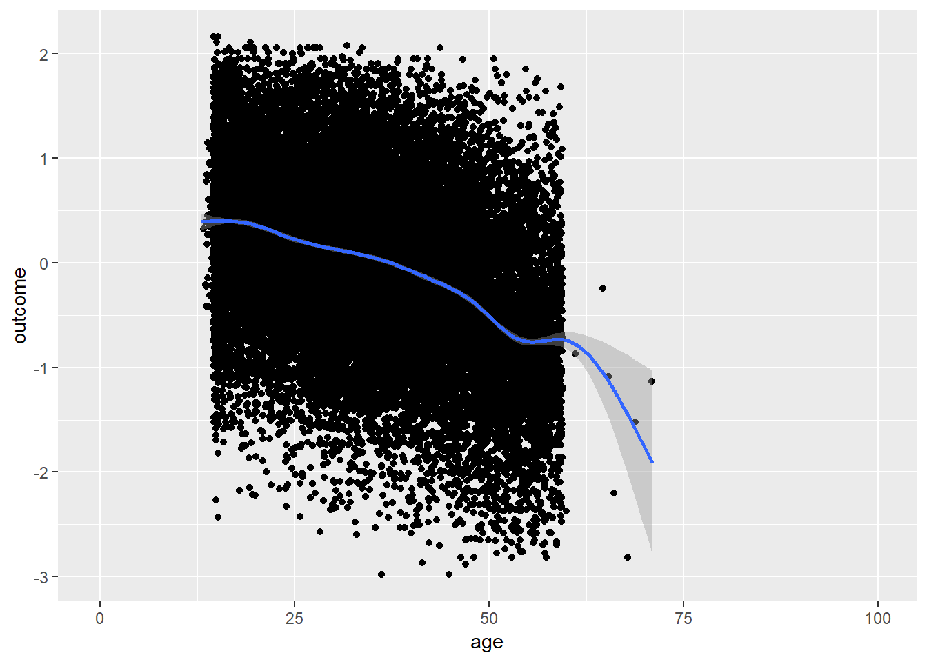

birthorder = birthorder %>%
  mutate(outcome = g_factor_2015_young)
plot_age(birthorder)

## `geom_smooth()` using method = 'gam' and formula 'y ~ s(x, bs = "cs")'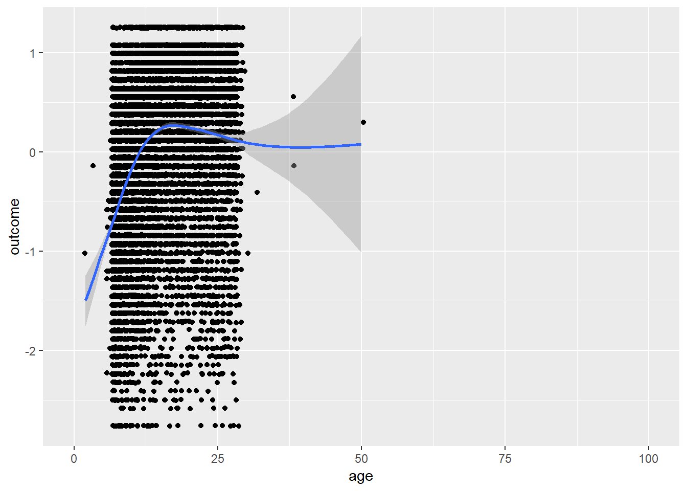

birthorder = birthorder %>%
  mutate(outcome = g_factor_2007_old)
plot_age(birthorder)

## `geom_smooth()` using method = 'gam' and formula 'y ~ s(x, bs = "cs")'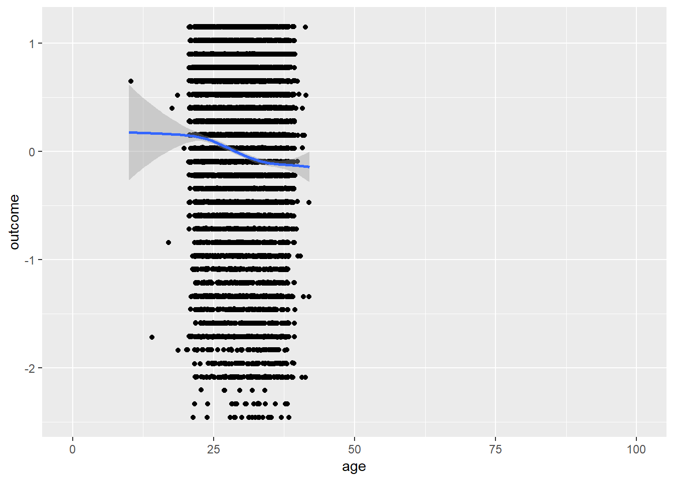

birthorder = birthorder %>%
  mutate(outcome = g_factor_2007_young)
plot_age(birthorder)

## `geom_smooth()` using method = 'gam' and formula 'y ~ s(x, bs = "cs")'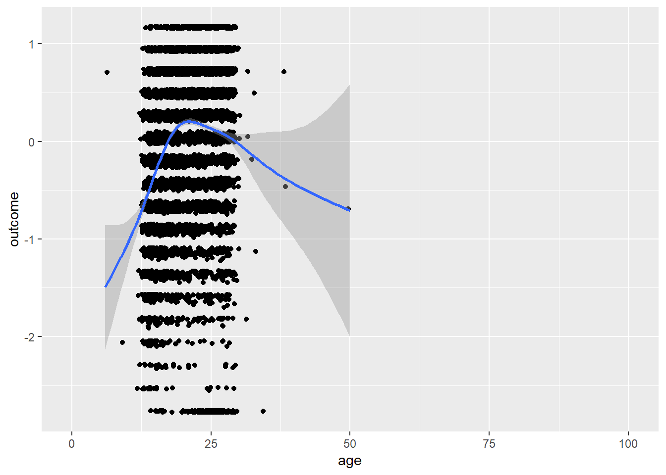

birthorder = birthorder %>%
  mutate(outcome = big5_ext)
plot_age(birthorder)

## `geom_smooth()` using method = 'gam' and formula 'y ~ s(x, bs = "cs")'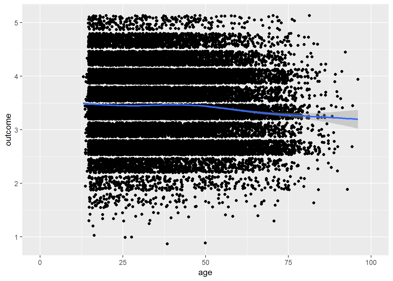

birthorder = birthorder %>%
  mutate(outcome = big5_con)
plot_age(birthorder)

## `geom_smooth()` using method = 'gam' and formula 'y ~ s(x, bs = "cs")'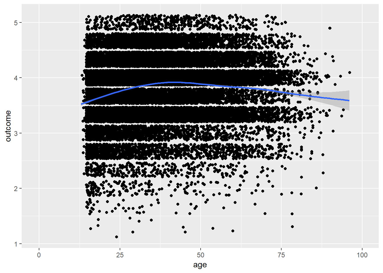

birthorder = birthorder %>%
  mutate(outcome = big5_open)
plot_age(birthorder)

## `geom_smooth()` using method = 'gam' and formula 'y ~ s(x, bs = "cs")'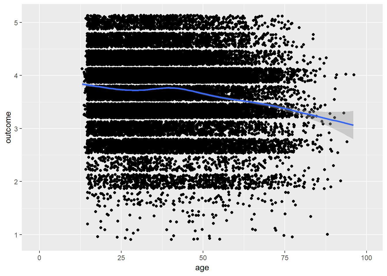

birthorder = birthorder %>%
  mutate(outcome = big5_neu)
plot_age(birthorder)

## `geom_smooth()` using method = 'gam' and formula 'y ~ s(x, bs = "cs")'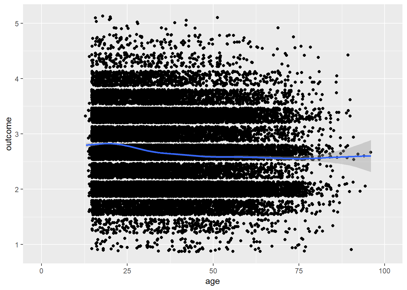

birthorder = birthorder %>%
  mutate(outcome = big5_agree)
plot_age(birthorder)

## `geom_smooth()` using method = 'gam' and formula 'y ~ s(x, bs = "cs")'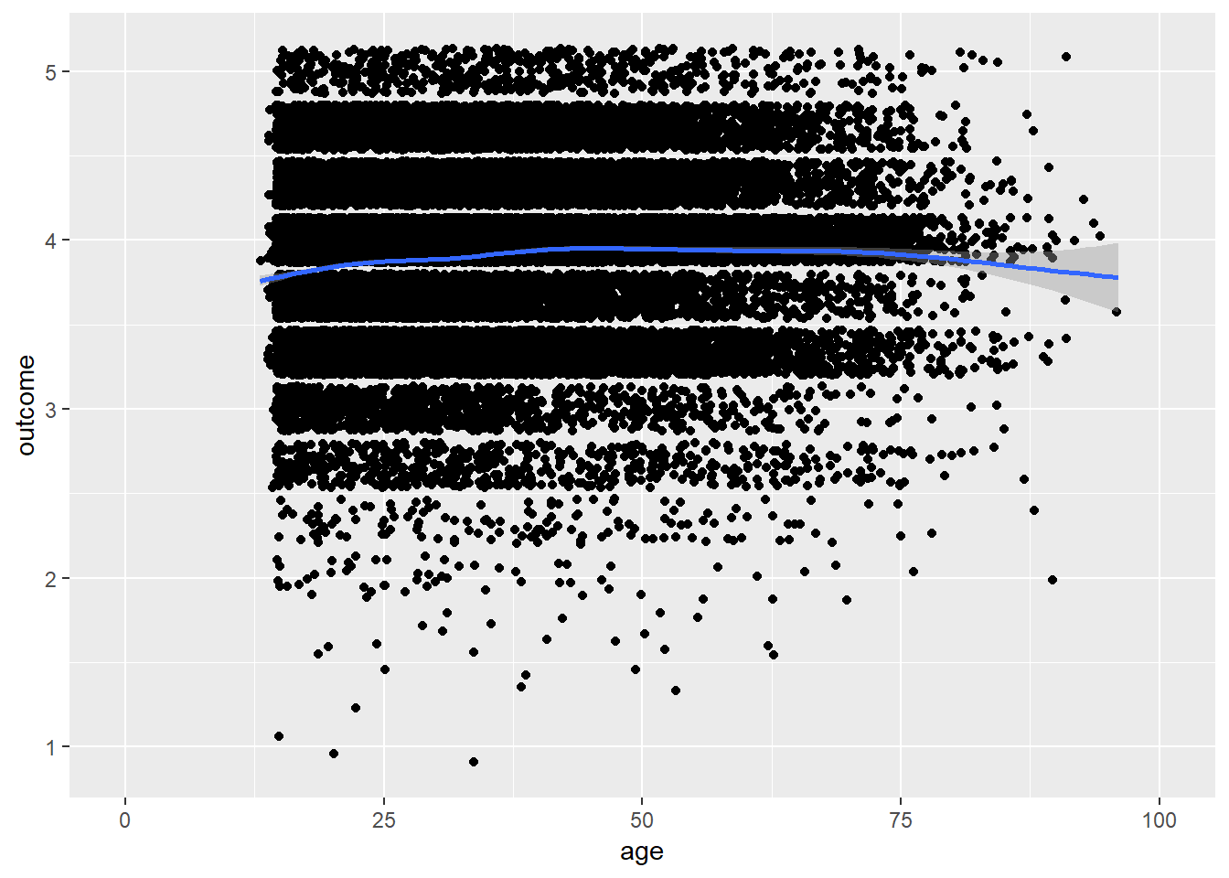

birthorder = birthorder %>%
  mutate(outcome = riskA)
plot_age(birthorder)

## `geom_smooth()` using method = 'gam' and formula 'y ~ s(x, bs = "cs")'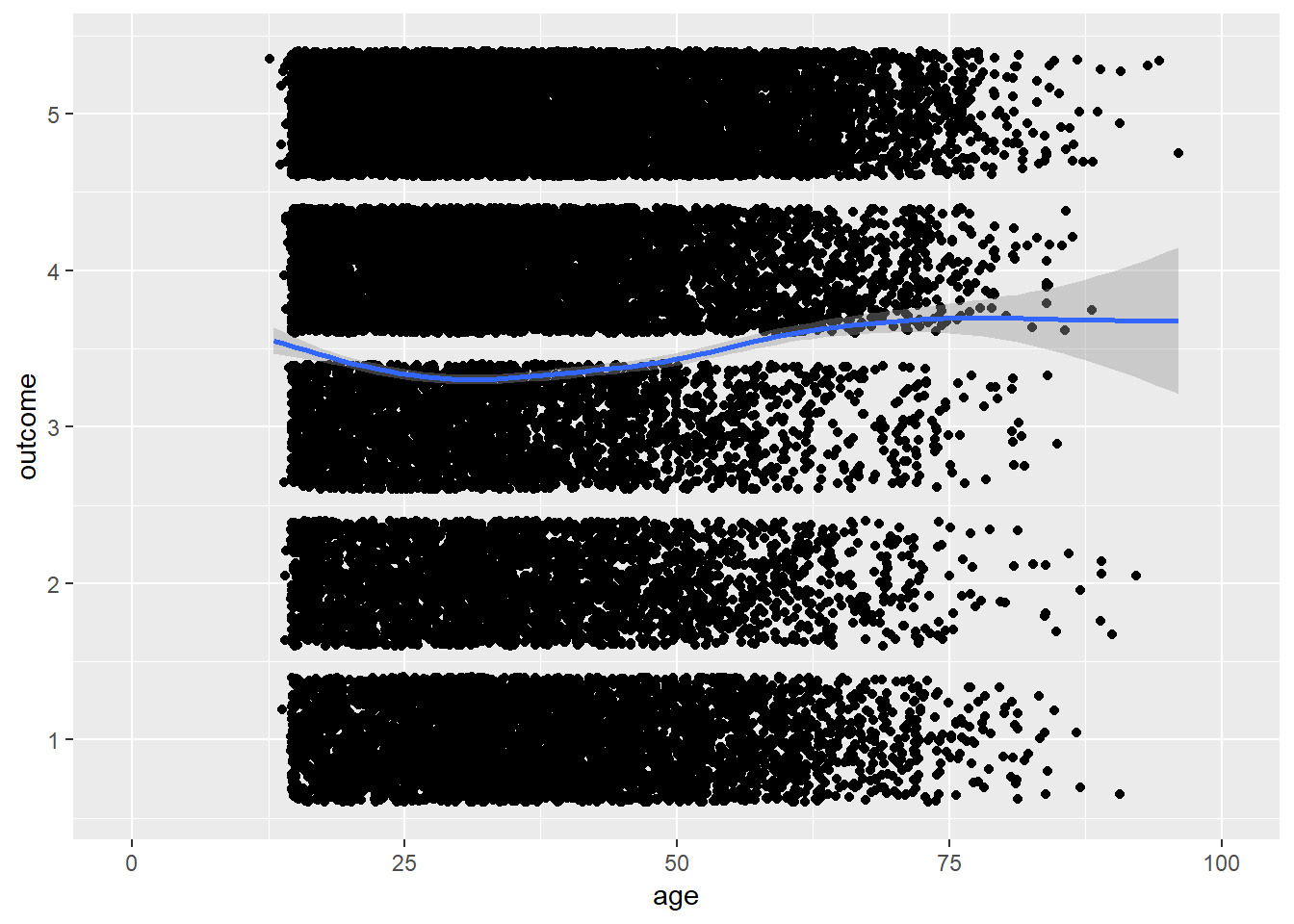

birthorder = birthorder %>%
  mutate(outcome = riskB)
plot_age(birthorder)

## `geom_smooth()` using method = 'gam' and formula 'y ~ s(x, bs = "cs")'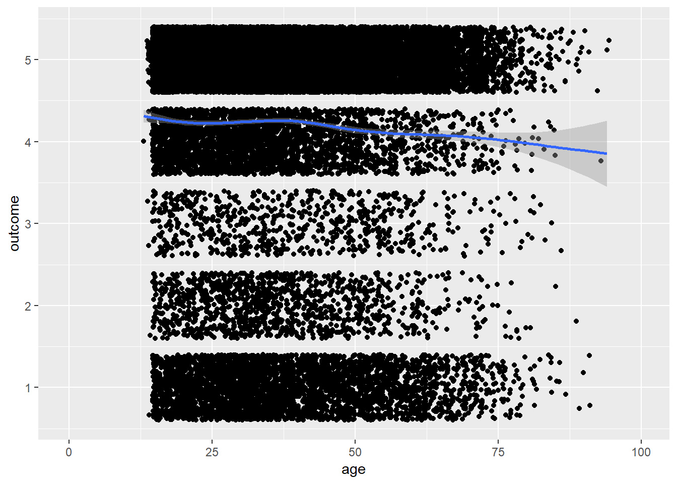

birthorder = birthorder %>%
  mutate(outcome = years_of_education)
plot_age(birthorder)

## `geom_smooth()` using method = 'gam' and formula 'y ~ s(x, bs = "cs")'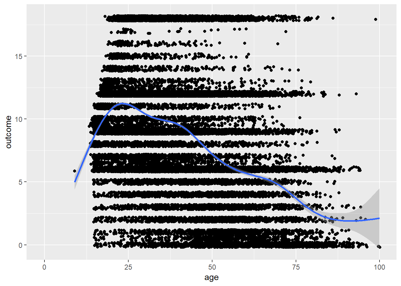

plot_age(birthorder %>% filter(!is.na(attended_school)) %>% mutate(outcome = as.numeric(attended_school)))

## `geom_smooth()` using method = 'gam' and formula 'y ~ s(x, bs = "cs")'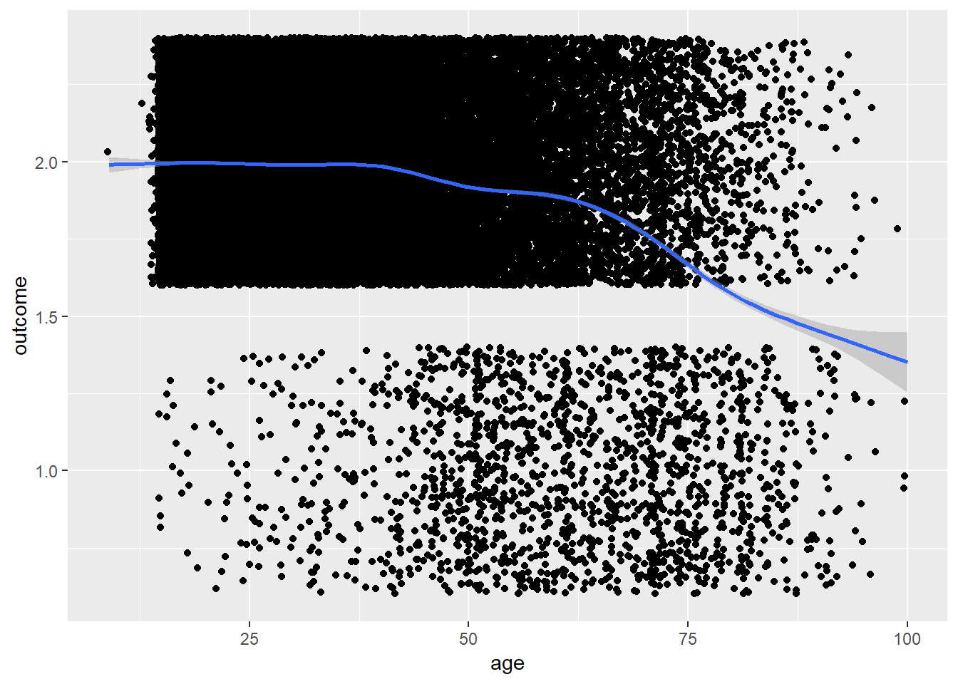

birthorder = birthorder %>%
  mutate(outcome = Elementary_missed)
plot_age(birthorder)

## `geom_smooth()` using method = 'gam' and formula 'y ~ s(x, bs = "cs")'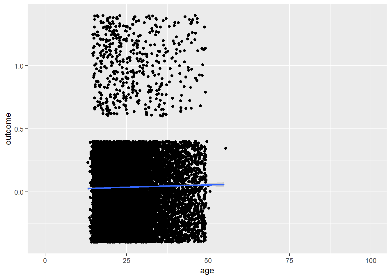

birthorder = birthorder %>%
  mutate(outcome = Elementary_worked)
plot_age(birthorder)

## `geom_smooth()` using method = 'gam' and formula 'y ~ s(x, bs = "cs")'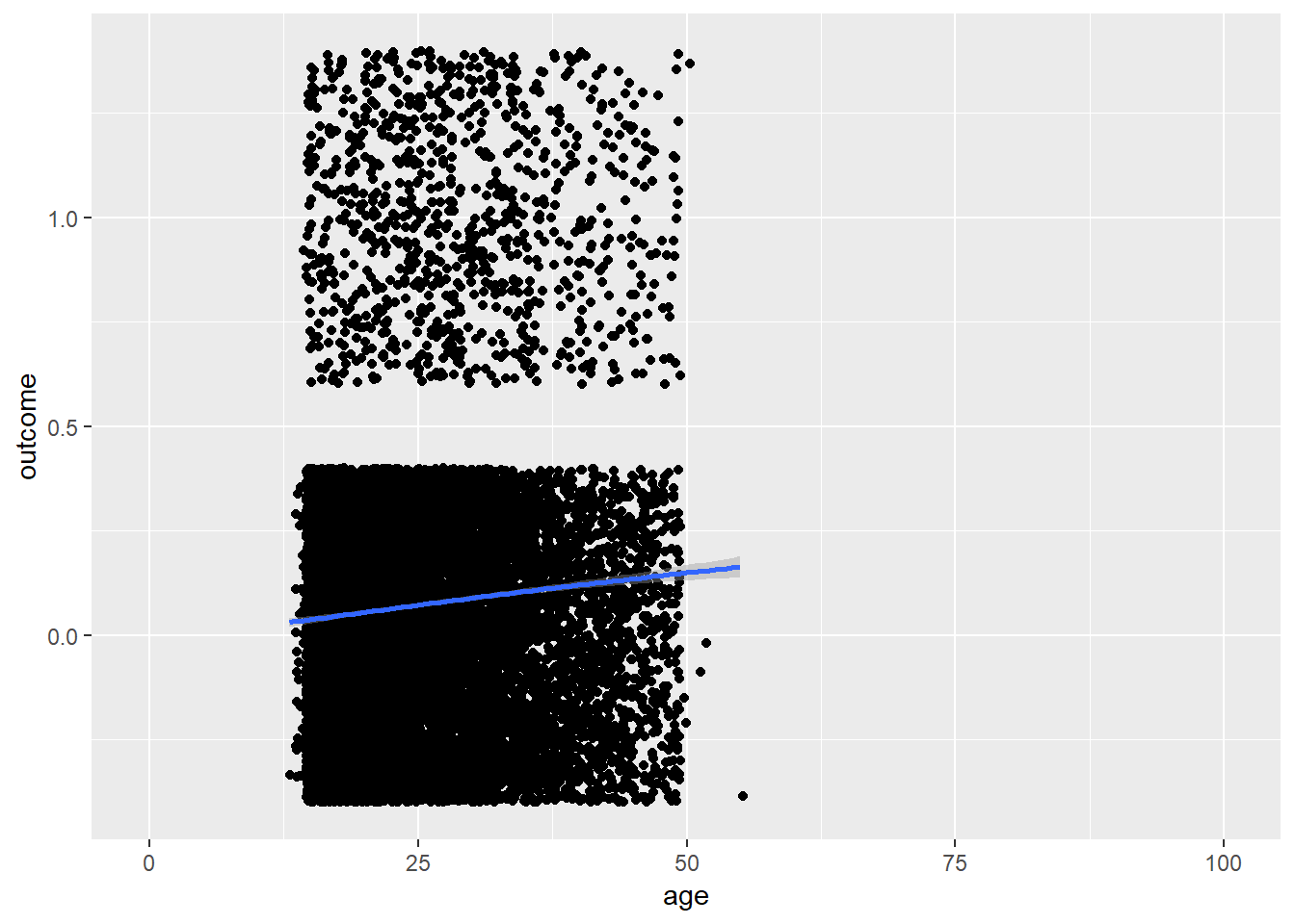

birthorder = birthorder %>%
  mutate(outcome = wage_last_month_log)
plot_age(birthorder)

## `geom_smooth()` using method = 'gam' and formula 'y ~ s(x, bs = "cs")'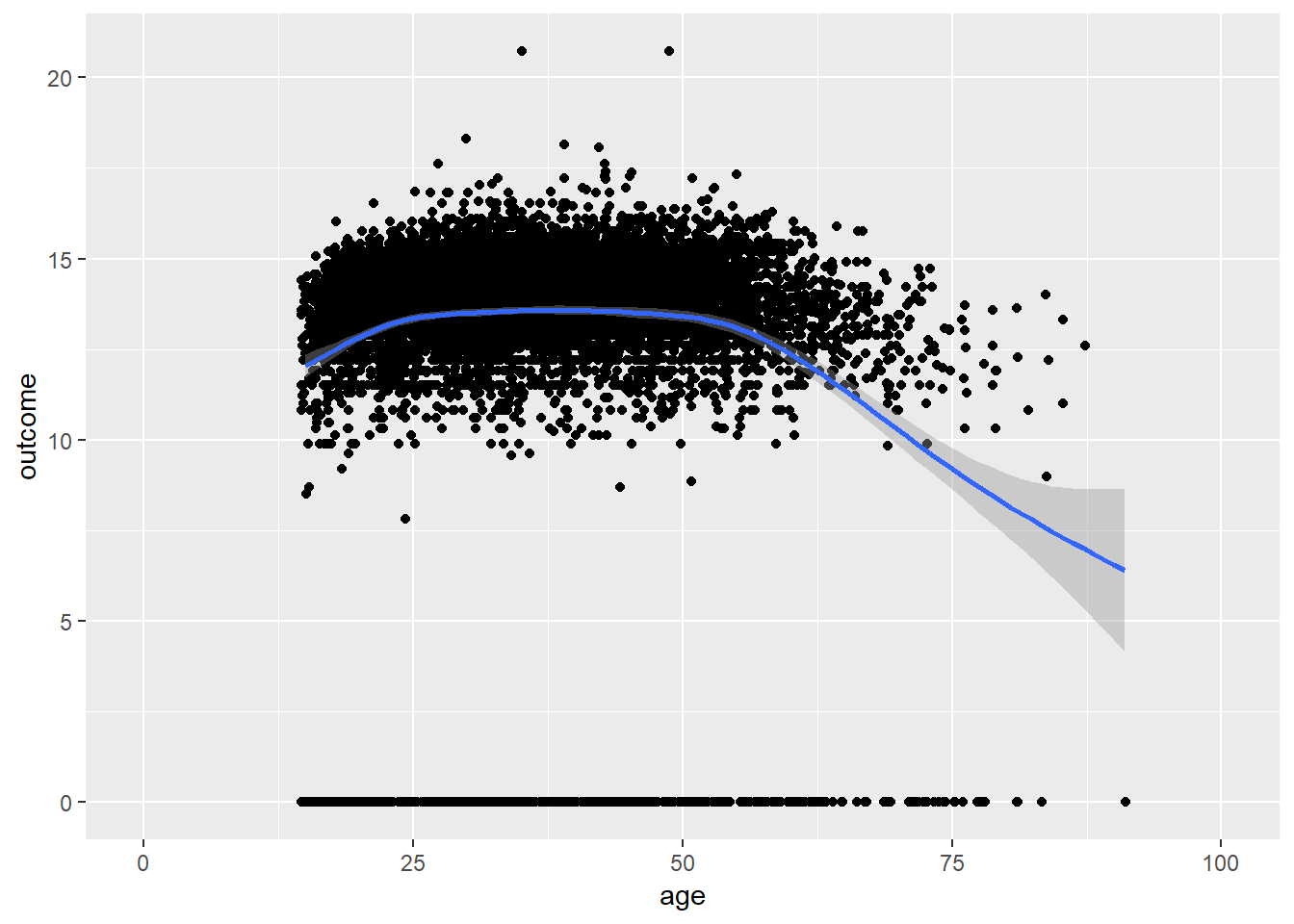

birthorder = birthorder %>%
  mutate(outcome = wage_last_year_log)
plot_age(birthorder)

## `geom_smooth()` using method = 'gam' and formula 'y ~ s(x, bs = "cs")'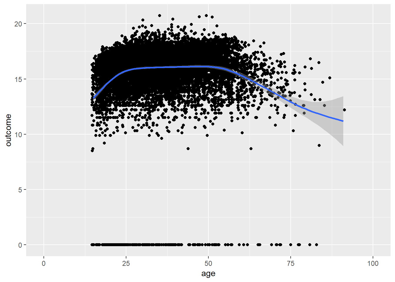

birthorder = birthorder %>%
  mutate(outcome = Self_employed)
plot_age(birthorder)

## `geom_smooth()` using method = 'gam' and formula 'y ~ s(x, bs = "cs")'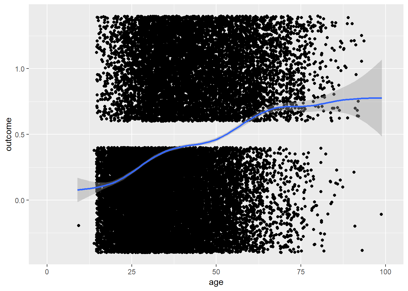

birthorder = birthorder %>%
  mutate(outcome = ever_smoked)
plot_age(birthorder)

## `geom_smooth()` using method = 'gam' and formula 'y ~ s(x, bs = "cs")'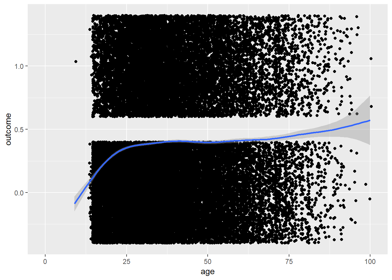

LS0tCnRpdGxlOiAiM19zYW1wbGVfYW5hbHlzZXMiCmF1dGhvcjogIkxhdXJhIEJvdHpldCAmIFJ1YmVuIEFyc2xhbiIKb3V0cHV0OiBodG1sX2RvY3VtZW50CmVkaXRvcl9vcHRpb25zOiAKICBjaHVua19vdXRwdXRfdHlwZTogY29uc29sZQotLS0KIyAgPHNwYW4gc3R5bGU9ImNvbG9yOiNFNzhBQzMiPlNhbXBsZSBBbmFseXNlczwvc3Bhbj4gey50YWJzZXR9CgojIyBIZWxwZXIKYGBge3IgaGVscGVyfQpzb3VyY2UoIjBfaGVscGVycy5SIikKYGBgCgojIyBMb2FkIGRhdGEKYGBge3IgTG9hZCBkYXRhfQojIyMgSW1wb3J0IGFsbCBkYXRhIHdpdGgga25vd24gYmlydGhvcmRlcgpiaXJ0aG9yZGVyID0gcmVhZFJEUygiZGF0YS9hbGxkYXRhX2JpcnRob3JkZXIucmRzIikKYGBgCgojIyBPdmVydmlldyBSYXcgZGF0YQpgYGB7ciBPdmVydmlldyBSYXcgRGF0YX0KIyBjb2RlYm9vayhiaXJ0aG9yZGVyKQpgYGAKCiMjIERhdGEgd3JhbmdsaW5nCmBgYHtyIGRhdGEgd3JhbmdsaW5nfQojIyB3ZSBoYXZlIHRvIGV4Y2x1ZGUgcGVvcGxlIGluIHRoZSBjb250cm9sIGdyb3VwIHdobyBhcmUgcGFydCBvZiB0aGUgYmlydGhvcmRlciBncm91cApiaXJ0aG9yZGVyID0gYmlydGhvcmRlciAlPiUKICAjIG1hcmsgcGVvcGxlIHdobyBoYXZlIG1pc3NpbmcgYmlydGhvcmRlciBkYXRhCiAgbXV0YXRlKGNoZWNrX2JpcnRob3JkZXIgPSBpZmVsc2UoIWlzLm5hKGJpcnRob3JkZXJfZ2VuZXMpLCAxLCAwKSwKICAjIG1hcmsgcGVvcGxlIHdobyBoYXZlIG1pc3Npbmcgb3V0Y29tZXMKICAgICAgICAgY2hlY2tfb3V0Y29tZSA9IGlmZWxzZSghaXMubmEocmF2ZW5fMjAxNV9vbGQpLCAxLAogICAgICAgICAgICAgICAgICAgICAgICAgaWZlbHNlKCFpcy5uYShtYXRoXzIwMTVfb2xkKSwgMSwKICAgICAgICAgICAgICAgICAgICAgICAgIGlmZWxzZSghaXMubmEocmF2ZW5fMjAxNV95b3VuZyksIDEsCiAgICAgICAgICAgICAgICAgICAgICAgICBpZmVsc2UoIWlzLm5hKG1hdGhfMjAxNV95b3VuZyksIDEsCiAgICAgICAgICAgICAgICAgICAgICAgICBpZmVsc2UoIWlzLm5hKHJhdmVuXzIwMDdfb2xkKSwgMSwKICAgICAgICAgICAgICAgICAgICAgICAgIGlmZWxzZSghaXMubmEobWF0aF8yMDA3X29sZCksIDEsCiAgICAgICAgICAgICAgICAgICAgICAgICBpZmVsc2UoIWlzLm5hKHJhdmVuXzIwMDdfeW91bmcpLCAxLAogICAgICAgICAgICAgICAgICAgICAgICAgaWZlbHNlKCFpcy5uYShtYXRoXzIwMDdfeW91bmcpLCAxLAogICAgICAgICAgICAgICAgICAgICAgICAgaWZlbHNlKCFpcy5uYShhZGFwdGl2ZV9udW1iZXJpbmcpLCAxLAogICAgICAgICAgICAgICAgICAgICAgICAgaWZlbHNlKCFpcy5uYSh3b3Jkc19yZW1lbWJlcmVkX2F2ZyksIDEsCiAgICAgICAgICAgICAgICAgICAgICAgICBpZmVsc2UoIWlzLm5hKGNvdW50X2JhY2t3YXJkcyksIDEsCiAgICAgICAgICAgICAgICAgICAgICAgICBpZmVsc2UoIWlzLm5hKGJpZzVfZXh0KSwgMSwgCiAgICAgICAgICAgICAgICAgICAgICAgICBpZmVsc2UoIWlzLm5hKHJpc2tBKSwgMSwKICAgICAgICAgICAgICAgICAgICAgICAgIGlmZWxzZSghaXMubmEocmlza0IpLCAxLAogICAgICAgICAgICAgICAgICAgICAgICAgaWZlbHNlKCFpcy5uYSh5ZWFyc19vZl9lZHVjYXRpb24pLCAxLAogICAgICAgICAgICAgICAgICAgICAgICAgaWZlbHNlKCFpcy5uYShFbGVtZW50YXJ5X21pc3NlZCksIDEsCiAgICAgICAgICAgICAgICAgICAgICAgICBpZmVsc2UoIWlzLm5hKEVsZW1lbnRhcnlfd29ya2VkKSwgMSwKICAgICAgICAgICAgICAgICAgICAgICAgIGlmZWxzZSghaXMubmEoYXR0ZW5kZWRfc2Nob29sKSwgMSwKICAgICAgICAgICAgICAgICAgICAgICAgIGlmZWxzZSghaXMubmEod2FnZV9sYXN0X21vbnRoX2xvZyksIDEsCiAgICAgICAgICAgICAgICAgICAgICAgICBpZmVsc2UoIWlzLm5hKHdhZ2VfbGFzdF95ZWFyX2xvZyksIDEsCiAgICAgICAgICAgICAgICAgICAgICAgICBpZmVsc2UoIWlzLm5hKFNlbGZfZW1wbG95ZWQpLCAxLAogICAgICAgICAgICAgICAgICAgICAgICAgaWZlbHNlKCFpcy5uYShDYXRlZ29yeSksIDEsCiAgICAgICAgICAgICAgICAgICAgICAgICBpZmVsc2UoIWlzLm5hKFNlY3RvciksIDEsCiAgICAgICAgICAgICAgICAgICAgICAgICBpZmVsc2UoIWlzLm5hKGV2ZXJfc21va2VkKSwgMSwKICAgICAgICAgICAgICAgICAgICAgICAgIGlmZWxzZSghaXMubmEoc3RpbGxfc21va2luZyksIDEsCiAgICAgICAgICAgICAgICAgICAgICAgICAwKSkpKSkpKSkpKSkpKSkpKSkpKSkpKSkpKSwKICBncm91cF9iaXJ0aG9yZGVyID0gaWZlbHNlKGNoZWNrX2JpcnRob3JkZXIgPT0gMCwgImNvbnRyb2wiLCAidGVzdCIpLAogIGdyb3VwX291dGNvbWUgPSBpZmVsc2UoY2hlY2tfb3V0Y29tZSA9PSAwLCAiY29udHJvbCIsICJ0ZXN0IikpCmBgYAoKIyMgQmlydGggb3JkZXIgYW5kIHNpYnNoaXAgc2l6ZSB7LmFjdGl2ZSAudGFic2V0fQoKIyMjIEdlbmVzIGJpcnRob3JkZXIKYGBge3IgbWF0ZXJuYWwgYmlydGhvcmRlcn0KZGVzY3JpcHRpdmVzID0gYmlydGhvcmRlciAlPiUKICBncm91cF9ieShncm91cF9vdXRjb21lKSAlPiUKICBzdW1tYXJpc2UoaW5kaXZpZHVhbHMgPSBuKCksCiAgICAgICAgICAgIG1vdGhlcnMgPSBsZW5ndGgodW5pcXVlKG1vdGhlcl9waWRsaW5rKSksCiAgICAgICAgICAgIHNpYnNoaXBfc2l6ZV9tZWFuID0gbWVhbihzaWJsaW5nX2NvdW50X2dlbmVzLCBuYS5ybSA9IFQpLAogICAgICAgICAgICBzaWJzaGlwX3NpemVfY29uZmlkZW5jZV9sb3cgPSBtZWFuKHNpYmxpbmdfY291bnRfZ2VuZXMsIG5hLnJtID0gVCkgLSAKICAgICAgICAgICAgICAocXQoLjk3NSwgbigpLTEpKnNkKHNpYmxpbmdfY291bnRfZ2VuZXMsIG5hLnJtID0gVCkvc3FydChuKCkpKSwKICAgICAgICAgICAgc2lic2hpcF9zaXplX2NvbmZpZGVuY2VfaGlnaCA9IG1lYW4oc2libGluZ19jb3VudF9nZW5lcywgbmEucm0gPSBUKSArIAogICAgICAgICAgICAgIChxdCguOTc1LCBuKCktMSkqc2Qoc2libGluZ19jb3VudF9nZW5lcywgbmEucm0gPSBUKS9zcXJ0KG4oKSkpLAogICAgICAgICAgICBzaWJzaGlwX3NpemVfbWluID0gbWluKHNpYmxpbmdfY291bnRfZ2VuZXMsIG5hLnJtID0gVFJVRSksCiAgICAgICAgICAgIHNpYnNoaXBfc2l6ZV9tYXggPSBtYXgoc2libGluZ19jb3VudF9nZW5lcywgbmEucm0gPSBUUlVFKSwKICAgICAgICAgICAgYmlydGhvcmRlcl9tZWFuID0gbWVhbihiaXJ0aG9yZGVyX2dlbmVzLCBuYS5ybSA9IFQpLAogICAgICAgICAgICBiaXJ0aG9yZGVyX3NpemVfY29uZmlkZW5jZV9sb3cgPSBtZWFuKGJpcnRob3JkZXJfZ2VuZXMsIG5hLnJtID0gVCkgLSAKICAgICAgICAgICAgICAocXQoLjk3NSwgbigpLTEpKnNkKGJpcnRob3JkZXJfZ2VuZXMsIG5hLnJtID0gVCkvc3FydChuKCkpKSwKICAgICAgICAgICAgYmlydGhvcmRlcl9zaXplX2NvbmZpZGVuY2VfaGlnaCA9IG1lYW4oYmlydGhvcmRlcl9nZW5lcywgbmEucm0gPSBUKSArIAogICAgICAgICAgICAgIChxdCguOTc1LCBuKCktMSkqc2QoYmlydGhvcmRlcl9nZW5lcywgbmEucm0gPSBUKS9zcXJ0KG4oKSkpLAogICAgICAgICAgICBiaXJ0aG9yZGVyX3NpemVfbWluID0gbWluKGJpcnRob3JkZXJfZ2VuZXMsIG5hLnJtID0gVFJVRSksCiAgICAgICAgICAgIGJpcnRob3JkZXJfc2l6ZV9tYXggPSBtYXgoYmlydGhvcmRlcl9nZW5lcywgbmEucm0gPSBUUlVFKSwKICAgICAgICAgICAgbnVtYmVyX3NpYmxpbmdzX21lYW4gPSBtZWFuKHNpYmxpbmdfY291bnRfZ2VuZXMsIG5hLnJtID1UKSwKICAgICAgICAgICAgbnVtYmVyX3NpYmxpbmdzX2NvbmZpZGVuY2VfbG93ID0gbWVhbihzaWJsaW5nX2NvdW50X2dlbmVzLCBuYS5ybSA9IFQpIC0KICAgICAgICAgICAgICAocXQoLjk3NSwgbigpLTEpKnNkKHNpYmxpbmdfY291bnRfZ2VuZXMsIG5hLnJtID0gVCkvc3FydChuKCkpKSwKICAgICAgICAgICAgbnVtYmVyX3NpYmxpbmdzX2NvbmZpZGVuY2VfaGlnaCA9IG1lYW4oc2libGluZ19jb3VudF9nZW5lcywgbmEucm0gPSBUKSArCiAgICAgICAgICAgICAgKHF0KC45NzUsIG4oKS0xKSpzZChzaWJsaW5nX2NvdW50X2dlbmVzLCBuYS5ybSA9IFQpL3NxcnQobigpKSkpCgpkZXNjcmlwdGl2ZXMKCmJpcnRob3JkZXIgJT4lIAogIHQudGVzdChzaWJsaW5nX2NvdW50X2dlbmVzIH4gZ3JvdXBfb3V0Y29tZSwgZGF0YSA9IC4sIHZhci5lcXVhbCA9IFQpCgpiaXJ0aG9yZGVyICU+JSAKICB0LnRlc3QoYmlydGhvcmRlcl9nZW5lcyB+IGdyb3VwX291dGNvbWUsIGRhdGEgPSAuLCB2YXIuZXF1YWwgPSBUKQoKYGBgCgoKIyMjIyBIb3cgbWFueSBzaWJsaW5ncyB3aXRoIGRhdGEgZG8gd2UgcmV0YWluIGluIGVhY2ggZmFtaWx5PwpgYGB7cn0KYmlydGhvcmRlciAlPiUgZmlsdGVyKCFpcy5uYShiaXJ0aG9yZGVyX2dlbmVzKSwgZ3JvdXBfb3V0Y29tZSA9PSAidGVzdCIpICU+JSBncm91cF9ieShtb3RoZXJfcGlkbGluaykgJT4lIHN1bW1hcmlzZSh3aXRoX2RhdGEgPSBuKCksIGFsbCA9IG1lYW4oc2libGluZ19jb3VudF9nZW5lcykpIC0+IGNvdW50cwpiaXJ0aG9yZGVyICU+JSBmaWx0ZXIoIWlzLm5hKGJpcnRob3JkZXJfZ2VuZXMpLCBncm91cF9vdXRjb21lID09ICJjb250cm9sIikgJT4lIGdyb3VwX2J5KG1vdGhlcl9waWRsaW5rKSAlPiUgc3VtbWFyaXNlKHdpdGhfZGF0YSA9IG4oKSwgYWxsID0gbWVhbihzaWJsaW5nX2NvdW50X2dlbmVzKSkgLT4gY291bnRzMQpgYGAKCkluIG91ciB0ZXN0IHNhbXBsZSBmYW1pbGllcyB3aXRoIGFuIGF2ZXJhZ2Ugc2l6ZSBvZiBgciBtZWFuKGNvdW50cyRhbGwsbmEucm09IFQpYCBzaWJsaW5ncywgd2UgcmV0YWluIGByIG1lYW4oY291bnRzJHdpdGhfZGF0YSlgLgoKSW4gdGhlIG9yaWdpbmFsIHNhbXBsZSBmYW1pbGllcyB3aXRoIGFuIGF2ZXJhZ2Ugc2l6ZSBvZiBgciBtZWFuKGNvdW50czEkYWxsLG5hLnJtPSBUKWAgc2libGluZ3MsIHdlIHJldGFpbiBgciBtZWFuKGNvdW50czEkd2l0aF9kYXRhKWAuCgpgYGB7cn0KZ2dwbG90KGNvdW50cywgYWVzKGFsbCwgd2l0aF9kYXRhKSkgKyBnZW9tX2ppdHRlcihhbHBoYSA9IDAuMSkgKyBnZW9tX3Ntb290aCgpICsgc2NhbGVfeF9jb250aW51b3VzKGJyZWFrcz0xOjE1KSArIHNjYWxlX3lfY29udGludW91cyhicmVha3M9MToxNSkKYGBgCgojIyMgTWF0ZXJuYWwgYmlydGhvcmRlcgpgYGB7ciBtYXRlcm5hbCBiaXJ0aG9yZGVyfQpkZXNjcmlwdGl2ZXMgPSBiaXJ0aG9yZGVyICU+JQogIGdyb3VwX2J5KGdyb3VwX291dGNvbWUpICU+JQogIHN1bW1hcmlzZShpbmRpdmlkdWFscyA9IG4oKSwKICAgICAgICAgICAgbW90aGVycyA9IGxlbmd0aCh1bmlxdWUobW90aGVyX3BpZGxpbmspKSwKICAgICAgICAgICAgc2lic2hpcF9zaXplX21lYW4gPSBtZWFuKHNpYmxpbmdfY291bnRfdXRlcnVzX2FsaXZlLCBuYS5ybSA9IFQpLAogICAgICAgICAgICBzaWJzaGlwX3NpemVfY29uZmlkZW5jZV9sb3cgPSBtZWFuKHNpYmxpbmdfY291bnRfdXRlcnVzX2FsaXZlLCBuYS5ybSA9IFQpIC0gCiAgICAgICAgICAgICAgKHF0KC45NzUsIG4oKS0xKSpzZChzaWJsaW5nX2NvdW50X3V0ZXJ1c19hbGl2ZSwgbmEucm0gPSBUKS9zcXJ0KG4oKSkpLAogICAgICAgICAgICBzaWJzaGlwX3NpemVfY29uZmlkZW5jZV9oaWdoID0gbWVhbihzaWJsaW5nX2NvdW50X3V0ZXJ1c19hbGl2ZSwgbmEucm0gPSBUKSArIAogICAgICAgICAgICAgIChxdCguOTc1LCBuKCktMSkqc2Qoc2libGluZ19jb3VudF91dGVydXNfYWxpdmUsIG5hLnJtID0gVCkvc3FydChuKCkpKSwKICAgICAgICAgICAgc2lic2hpcF9zaXplX21pbiA9IG1pbihzaWJsaW5nX2NvdW50X3V0ZXJ1c19hbGl2ZSwgbmEucm0gPSBUUlVFKSwKICAgICAgICAgICAgc2lic2hpcF9zaXplX21heCA9IG1heChzaWJsaW5nX2NvdW50X3V0ZXJ1c19hbGl2ZSwgbmEucm0gPSBUUlVFKSwKICAgICAgICAgICAgYmlydGhvcmRlcl9tZWFuID0gbWVhbihiaXJ0aG9yZGVyX3V0ZXJ1c19hbGl2ZSwgbmEucm0gPSBUKSwKICAgICAgICAgICAgYmlydGhvcmRlcl9zaXplX2NvbmZpZGVuY2VfbG93ID0gbWVhbihiaXJ0aG9yZGVyX3V0ZXJ1c19hbGl2ZSwgbmEucm0gPSBUKSAtIAogICAgICAgICAgICAgIChxdCguOTc1LCBuKCktMSkqc2QoYmlydGhvcmRlcl91dGVydXNfYWxpdmUsIG5hLnJtID0gVCkvc3FydChuKCkpKSwKICAgICAgICAgICAgYmlydGhvcmRlcl9zaXplX2NvbmZpZGVuY2VfaGlnaCA9IG1lYW4oYmlydGhvcmRlcl91dGVydXNfYWxpdmUsIG5hLnJtID0gVCkgKyAKICAgICAgICAgICAgICAocXQoLjk3NSwgbigpLTEpKnNkKGJpcnRob3JkZXJfdXRlcnVzX2FsaXZlLCBuYS5ybSA9IFQpL3NxcnQobigpKSksCiAgICAgICAgICAgIGJpcnRob3JkZXJfc2l6ZV9taW4gPSBtaW4oYmlydGhvcmRlcl91dGVydXNfYWxpdmUsIG5hLnJtID0gVFJVRSksCiAgICAgICAgICAgIGJpcnRob3JkZXJfc2l6ZV9tYXggPSBtYXgoYmlydGhvcmRlcl91dGVydXNfYWxpdmUsIG5hLnJtID0gVFJVRSksCiAgICAgICAgICAgIG51bWJlcl9zaWJsaW5nc19tZWFuID0gbWVhbihzaWJsaW5nX2NvdW50X3V0ZXJ1c19hbGl2ZSwgbmEucm0gPVQpLAogICAgICAgICAgICBudW1iZXJfc2libGluZ3NfY29uZmlkZW5jZV9sb3cgPSBtZWFuKHNpYmxpbmdfY291bnRfdXRlcnVzX2FsaXZlLCBuYS5ybSA9IFQpIC0KICAgICAgICAgICAgICAocXQoLjk3NSwgbigpLTEpKnNkKHNpYmxpbmdfY291bnRfdXRlcnVzX2FsaXZlLCBuYS5ybSA9IFQpL3NxcnQobigpKSksCiAgICAgICAgICAgIG51bWJlcl9zaWJsaW5nc19jb25maWRlbmNlX2hpZ2ggPSBtZWFuKHNpYmxpbmdfY291bnRfdXRlcnVzX2FsaXZlLCBuYS5ybSA9IFQpICsKICAgICAgICAgICAgICAocXQoLjk3NSwgbigpLTEpKnNkKHNpYmxpbmdfY291bnRfdXRlcnVzX2FsaXZlLCBuYS5ybSA9IFQpL3NxcnQobigpKSkpCgpkZXNjcmlwdGl2ZXMKCmJpcnRob3JkZXIgJT4lIAogIHQudGVzdChzaWJsaW5nX2NvdW50X3V0ZXJ1c19hbGl2ZSB+IGdyb3VwX291dGNvbWUsIGRhdGEgPSAuLCB2YXIuZXF1YWwgPSBUKQoKYmlydGhvcmRlciAlPiUgCiAgdC50ZXN0KGJpcnRob3JkZXJfdXRlcnVzX2FsaXZlIH4gZ3JvdXBfb3V0Y29tZSwgZGF0YSA9IC4sIHZhci5lcXVhbCA9IFQpCgpgYGAKCgojIyMjIEhvdyBtYW55IHNpYmxpbmdzIHdpdGggZGF0YSBkbyB3ZSByZXRhaW4gaW4gZWFjaCBmYW1pbHk/CmBgYHtyfQoKYmlydGhvcmRlciAlPiUgZmlsdGVyKCFpcy5uYShiaXJ0aG9yZGVyX3V0ZXJ1c19hbGl2ZSksIGdyb3VwX291dGNvbWUgPT0gMSkgJT4lIGdyb3VwX2J5KG1vdGhlcl9waWRsaW5rKSAlPiUgc3VtbWFyaXNlKHdpdGhfZGF0YSA9IG4oKSwgYWxsID0gbWVhbihzaWJsaW5nX2NvdW50X3V0ZXJ1c19hbGl2ZSkpIC0+IGNvdW50cwpiaXJ0aG9yZGVyICU+JSBmaWx0ZXIoIWlzLm5hKGJpcnRob3JkZXJfdXRlcnVzX2FsaXZlKSwgZ3JvdXBfb3V0Y29tZSA9PSAwKSAlPiUgZ3JvdXBfYnkobW90aGVyX3BpZGxpbmspICU+JSBzdW1tYXJpc2Uod2l0aF9kYXRhID0gbigpLCBhbGwgPSBtZWFuKHNpYmxpbmdfY291bnRfdXRlcnVzX2FsaXZlKSkgLT4gY291bnRzMQpgYGAKCkluIG91ciB0ZXN0IHNhbXBsZSBmYW1pbGllcyB3aXRoIGFuIGF2ZXJhZ2Ugc2l6ZSBvZiBgciBtZWFuKGNvdW50cyRhbGwsbmEucm09IFQpYCBzaWJsaW5ncywgd2UgcmV0YWluIGByIG1lYW4oY291bnRzJHdpdGhfZGF0YSlgLgoKSW4gdGhlIG9yaWdpbmFsIHNhbXBsZSBmYW1pbGllcyB3aXRoIGFuIGF2ZXJhZ2Ugc2l6ZSBvZiBgciBtZWFuKGNvdW50czEkYWxsLG5hLnJtPSBUKWAgc2libGluZ3MsIHdlIHJldGFpbiBgciBtZWFuKGNvdW50czEkd2l0aF9kYXRhKWAuCgpgYGB7cn0KZ2dwbG90KGNvdW50cywgYWVzKGFsbCwgd2l0aF9kYXRhKSkgKyBnZW9tX2ppdHRlcihhbHBoYSA9IDAuMSkgKyBnZW9tX3Ntb290aCgpICsgc2NhbGVfeF9jb250aW51b3VzKGJyZWFrcz0xOjE1KSArIHNjYWxlX3lfY29udGludW91cyhicmVha3M9MToxNSkKYGBgCiMjIyBNYXRlcm5hbCBwcmVnbmFuY3kgYmlydGhvcmRlcgpgYGB7ciBtYXRlcm5hbCBiaXJ0aG9yZGVyfQpkZXNjcmlwdGl2ZXMgPSBiaXJ0aG9yZGVyICU+JQogIGdyb3VwX2J5KGdyb3VwX291dGNvbWUpICU+JQogIHN1bW1hcmlzZShpbmRpdmlkdWFscyA9IG4oKSwKICAgICAgICAgICAgbW90aGVycyA9IGxlbmd0aCh1bmlxdWUobW90aGVyX3BpZGxpbmspKSwKICAgICAgICAgICAgc2lic2hpcF9zaXplX21lYW4gPSBtZWFuKHNpYmxpbmdfY291bnRfdXRlcnVzX3ByZWcsIG5hLnJtID0gVCksCiAgICAgICAgICAgIHNpYnNoaXBfc2l6ZV9jb25maWRlbmNlX2xvdyA9IG1lYW4oc2libGluZ19jb3VudF91dGVydXNfcHJlZywgbmEucm0gPSBUKSAtIAogICAgICAgICAgICAgIChxdCguOTc1LCBuKCktMSkqc2Qoc2libGluZ19jb3VudF91dGVydXNfcHJlZywgbmEucm0gPSBUKS9zcXJ0KG4oKSkpLAogICAgICAgICAgICBzaWJzaGlwX3NpemVfY29uZmlkZW5jZV9oaWdoID0gbWVhbihzaWJsaW5nX2NvdW50X3V0ZXJ1c19wcmVnLCBuYS5ybSA9IFQpICsgCiAgICAgICAgICAgICAgKHF0KC45NzUsIG4oKS0xKSpzZChzaWJsaW5nX2NvdW50X3V0ZXJ1c19wcmVnLCBuYS5ybSA9IFQpL3NxcnQobigpKSksCiAgICAgICAgICAgIHNpYnNoaXBfc2l6ZV9taW4gPSBtaW4oc2libGluZ19jb3VudF91dGVydXNfcHJlZywgbmEucm0gPSBUUlVFKSwKICAgICAgICAgICAgc2lic2hpcF9zaXplX21heCA9IG1heChzaWJsaW5nX2NvdW50X3V0ZXJ1c19wcmVnLCBuYS5ybSA9IFRSVUUpLAogICAgICAgICAgICBiaXJ0aG9yZGVyX21lYW4gPSBtZWFuKGJpcnRob3JkZXJfdXRlcnVzX3ByZWcsIG5hLnJtID0gVCksCiAgICAgICAgICAgIGJpcnRob3JkZXJfc2l6ZV9jb25maWRlbmNlX2xvdyA9IG1lYW4oYmlydGhvcmRlcl91dGVydXNfcHJlZywgbmEucm0gPSBUKSAtIAogICAgICAgICAgICAgIChxdCguOTc1LCBuKCktMSkqc2QoYmlydGhvcmRlcl91dGVydXNfcHJlZywgbmEucm0gPSBUKS9zcXJ0KG4oKSkpLAogICAgICAgICAgICBiaXJ0aG9yZGVyX3NpemVfY29uZmlkZW5jZV9oaWdoID0gbWVhbihiaXJ0aG9yZGVyX3V0ZXJ1c19wcmVnLCBuYS5ybSA9IFQpICsgCiAgICAgICAgICAgICAgKHF0KC45NzUsIG4oKS0xKSpzZChiaXJ0aG9yZGVyX3V0ZXJ1c19wcmVnLCBuYS5ybSA9IFQpL3NxcnQobigpKSksCiAgICAgICAgICAgIGJpcnRob3JkZXJfc2l6ZV9taW4gPSBtaW4oYmlydGhvcmRlcl91dGVydXNfcHJlZywgbmEucm0gPSBUUlVFKSwKICAgICAgICAgICAgYmlydGhvcmRlcl9zaXplX21heCA9IG1heChiaXJ0aG9yZGVyX3V0ZXJ1c19wcmVnLCBuYS5ybSA9IFRSVUUpLAogICAgICAgICAgICBudW1iZXJfc2libGluZ3NfbWVhbiA9IG1lYW4oc2libGluZ19jb3VudF91dGVydXNfcHJlZywgbmEucm0gPVQpLAogICAgICAgICAgICBudW1iZXJfc2libGluZ3NfY29uZmlkZW5jZV9sb3cgPSBtZWFuKHNpYmxpbmdfY291bnRfdXRlcnVzX3ByZWcsIG5hLnJtID0gVCkgLQogICAgICAgICAgICAgIChxdCguOTc1LCBuKCktMSkqc2Qoc2libGluZ19jb3VudF91dGVydXNfcHJlZywgbmEucm0gPSBUKS9zcXJ0KG4oKSkpLAogICAgICAgICAgICBudW1iZXJfc2libGluZ3NfY29uZmlkZW5jZV9oaWdoID0gbWVhbihzaWJsaW5nX2NvdW50X3V0ZXJ1c19wcmVnLCBuYS5ybSA9IFQpICsKICAgICAgICAgICAgICAocXQoLjk3NSwgbigpLTEpKnNkKHNpYmxpbmdfY291bnRfdXRlcnVzX3ByZWcsIG5hLnJtID0gVCkvc3FydChuKCkpKSkKCmRlc2NyaXB0aXZlcwoKYmlydGhvcmRlciAlPiUgCiAgdC50ZXN0KHNpYmxpbmdfY291bnRfdXRlcnVzX3ByZWcgfiBncm91cF9vdXRjb21lLCBkYXRhID0gLiwgdmFyLmVxdWFsID0gVCkKCmJpcnRob3JkZXIgJT4lIAogIHQudGVzdChiaXJ0aG9yZGVyX3V0ZXJ1c19wcmVnIH4gZ3JvdXBfb3V0Y29tZSwgZGF0YSA9IC4sIHZhci5lcXVhbCA9IFQpCgpgYGAKCgojIyMjIEhvdyBtYW55IHNpYmxpbmdzIHdpdGggZGF0YSBkbyB3ZSByZXRhaW4gaW4gZWFjaCBmYW1pbHk/CmBgYHtyfQpiaXJ0aG9yZGVyICU+JSBmaWx0ZXIoIWlzLm5hKGJpcnRob3JkZXJfdXRlcnVzX3ByZWcpLCBncm91cF9vdXRjb21lID09IDEpICU+JSBncm91cF9ieShtb3RoZXJfcGlkbGluaykgJT4lIHN1bW1hcmlzZSh3aXRoX2RhdGEgPSBuKCksIGFsbCA9IG1lYW4oc2libGluZ19jb3VudF91dGVydXNfcHJlZykpIC0+IGNvdW50cwpiaXJ0aG9yZGVyICU+JSBmaWx0ZXIoIWlzLm5hKGJpcnRob3JkZXJfdXRlcnVzX3ByZWcpLCBncm91cF9vdXRjb21lID09IDApICU+JSBncm91cF9ieShtb3RoZXJfcGlkbGluaykgJT4lIHN1bW1hcmlzZSh3aXRoX2RhdGEgPSBuKCksIGFsbCA9IG1lYW4oc2libGluZ19jb3VudF91dGVydXNfcHJlZykpIC0+IGNvdW50czEKYGBgCgpJbiBvdXIgdGVzdCBzYW1wbGUgZmFtaWxpZXMgd2l0aCBhbiBhdmVyYWdlIHNpemUgb2YgYHIgbWVhbihjb3VudHMkYWxsLG5hLnJtPSBUKWAgc2libGluZ3MsIHdlIHJldGFpbiBgciBtZWFuKGNvdW50cyR3aXRoX2RhdGEpYC4KCkluIHRoZSBvcmlnaW5hbCBzYW1wbGUgZmFtaWxpZXMgd2l0aCBhbiBhdmVyYWdlIHNpemUgb2YgYHIgbWVhbihjb3VudHMxJGFsbCxuYS5ybT0gVClgIHNpYmxpbmdzLCB3ZSByZXRhaW4gYHIgbWVhbihjb3VudHMxJHdpdGhfZGF0YSlgLgoKYGBge3J9CmdncGxvdChjb3VudHMsIGFlcyhhbGwsIHdpdGhfZGF0YSkpICsgZ2VvbV9qaXR0ZXIoYWxwaGEgPSAwLjEpICsgZ2VvbV9zbW9vdGgoKSArIHNjYWxlX3hfY29udGludW91cyhicmVha3M9MToxNSkgKyBzY2FsZV95X2NvbnRpbnVvdXMoYnJlYWtzPTE6MTUpCmBgYAoKCiMjIE91dGNvbWUgbWVhc3VyZW1lbnRzIGFuZCBjb3ZhcmlhdGVzIHsudGFic2V0fQojIyMgQ29udHJvbCBncm91cApgYGB7ciBkYXRhIGNvbXBhcmlzb259CiMjIERlc2NyaXB0aXZlcwpkZXNjcmlwdGl2ZXMgPSBiaXJ0aG9yZGVyICU+JQogIGdyb3VwX2J5KGdyb3VwX2JpcnRob3JkZXIpICU+JQogICAgc3VtbWFyaXNlKG4gPSBuKCksCiAgICAgICAgICAgICAgYWdlX21lYW4gPSBtZWFuKGFnZSwgbmEucm09VFJVRSksCiAgICAgICAgICAgICAgYWdlX2NvbmZpZGVuY2VfbG93ID0gbWVhbihhZ2UsIG5hLnJtID0gVCkgLSAKICAgICAgICAgICAgICAgIChxdCguOTc1LCBuKCktMSkqc2QoYWdlLCBuYS5ybSA9IFQpL3NxcnQobigpKSksCiAgICAgICAgICAgICAgYWdlX2NvbmZpZGVuY2VfaGlnaCA9IG1lYW4oYWdlLCBuYS5ybSA9IFQpICsgCiAgICAgICAgICAgICAgICAocXQoLjk3NSwgbigpLTEpKnNkKGFnZSwgbmEucm0gPSBUKS9zcXJ0KG4oKSkpLAogICAgICAgICAgICAgIGFnZV9taW4gPSBtaW4oYWdlLCBuYS5ybSA9IFRSVUUpLAogICAgICAgICAgICAgIGFnZV9tYXggPSBtYXgoYWdlLCBuYS5ybSA9IFRSVUUpLAogICAgICAgICAgICAgIGdlbmRlciA9IG1lYW4obWFsZSwgbmEucm09VFJVRSkpCmRlc2NyaXB0aXZlcwoKCgojIyBUdGVzdAp0aWR5KHQudGVzdChiaXJ0aG9yZGVyJGFnZSB+IGJpcnRob3JkZXIkZ3JvdXBfYmlydGhvcmRlciwgdmFyLmVxdWFsID0gVCkpCgpjb2hlbi5kKGJpcnRob3JkZXIkYWdlLCBhcy5mYWN0b3IoYmlydGhvcmRlciRncm91cF9iaXJ0aG9yZGVyKSwgbmEucm0gPSBUKQoKZ2VuZGVyID0gYmlydGhvcmRlciAlPiUKICBncm91cF9ieShncm91cF9iaXJ0aG9yZGVyKSAlPiUKICAgIHN1bW1hcmlzZShnZW5kZXIgPSBzdW0obWFsZSA9PSAxLCBuYS5ybT1UKSwKICAgICAgICAgICAgICBnZW5kZXIyID0gc3VtKG1hbGUgPT0wLG5hLnJtPVQpKSAlPiUKICBzZWxlY3QoZ2VuZGVyLCBnZW5kZXIyKQpwcm9wLnRhYmxlKGdlbmRlcikKdGlkeShjaGlzcS50ZXN0KGdlbmRlcikpCgojIyBSYXRpbmdzCnJhdGluZ3MgPSBiaXJ0aG9yZGVyICU+JQogIGdyb3VwX2J5KGdyb3VwX2JpcnRob3JkZXIpICU+JQogIHN1bW1hcmlzZShnX2ZhY3Rvcl9tZWFuID0gbWVhbihnX2ZhY3Rvcl8yMDE1X29sZCwgbmEucm09VCksCiAgICAgICAgICAgIGdfZmFjdG9yX2NvbmZpZGVuY2VfbG93PSBtZWFuKGdfZmFjdG9yXzIwMTVfb2xkLCBuYS5ybSA9IFQpIC0gCiAgICAgICAgICAgICAgICAocXQoLjk3NSwgbigpLTEpKnNkKGdfZmFjdG9yXzIwMTVfb2xkLCBuYS5ybSA9IFQpL3NxcnQobigpKSksCiAgICAgICAgICAgIGdfZmFjdG9yX2NvbmZpZGVuY2VfaGlnaCA9IG1lYW4oZ19mYWN0b3JfMjAxNV9vbGQsIG5hLnJtID0gVCkgKwogICAgICAgICAgICAgICAgKHF0KC45NzUsIG4oKS0xKSpzZChnX2ZhY3Rvcl8yMDE1X29sZCwgbmEucm0gPSBUKS9zcXJ0KG4oKSkpLAogICAgICAgICAgICBiaWc1X2V4dF9tZWFuID0gbWVhbihiaWc1X2V4dCwgbmEucm09VCksCiAgICAgICAgICAgIGJpZzVfZXh0X2NvbmZpZGVuY2VfbG93PSBtZWFuKGJpZzVfZXh0LCBuYS5ybSA9IFQpIC0gCiAgICAgICAgICAgICAgICAocXQoLjk3NSwgbigpLTEpKnNkKGJpZzVfZXh0LCBuYS5ybSA9IFQpL3NxcnQobigpKSksCiAgICAgICAgICAgIGJpZzVfZXh0X2NvbmZpZGVuY2VfaGlnaCA9IG1lYW4oYmlnNV9leHQsIG5hLnJtID0gVCkgKwogICAgICAgICAgICAgICAgKHF0KC45NzUsIG4oKS0xKSpzZChiaWc1X2V4dCwgbmEucm0gPSBUKS9zcXJ0KG4oKSkpLAogICAgICAgICAgICBiaWc1X25ldV9tZWFuID0gbWVhbihiaWc1X25ldSwgbmEucm09VCksCiAgICAgICAgICAgIGJpZzVfbmV1X2NvbmZpZGVuY2VfbG93PSBtZWFuKGJpZzVfbmV1LCBuYS5ybSA9IFQpIC0gCiAgICAgICAgICAgICAgICAocXQoLjk3NSwgbigpLTEpKnNkKGJpZzVfbmV1LCBuYS5ybSA9IFQpL3NxcnQobigpKSksCiAgICAgICAgICAgIGJpZzVfbmV1X2NvbmZpZGVuY2VfaGlnaCA9IG1lYW4oYmlnNV9uZXUsIG5hLnJtID0gVCkgKwogICAgICAgICAgICAgICAgKHF0KC45NzUsIG4oKS0xKSpzZChiaWc1X25ldSwgbmEucm0gPSBUKS9zcXJ0KG4oKSkpLAogICAgICAgICAgICBiaWc1X2Nvbl9tZWFuID0gbWVhbihiaWc1X2NvbiwgbmEucm09VCksCiAgICAgICAgICAgIGJpZzVfY29uX2NvbmZpZGVuY2VfbG93PSBtZWFuKGJpZzVfY29uLCBuYS5ybSA9IFQpIC0gCiAgICAgICAgICAgICAgICAocXQoLjk3NSwgbigpLTEpKnNkKGJpZzVfY29uLCBuYS5ybSA9IFQpL3NxcnQobigpKSksCiAgICAgICAgICAgIGJpZzVfY29uX2NvbmZpZGVuY2VfaGlnaCA9IG1lYW4oYmlnNV9jb24sIG5hLnJtID0gVCkgKwogICAgICAgICAgICAgICAgKHF0KC45NzUsIG4oKS0xKSpzZChiaWc1X2NvbiwgbmEucm0gPSBUKS9zcXJ0KG4oKSkpLAogICAgICAgICAgICBiaWc1X2FncmVlX21lYW4gPSBtZWFuKGJpZzVfYWdyZWUsIG5hLnJtPVQpLAogICAgICAgICAgICBiaWc1X2FncmVlX2NvbmZpZGVuY2VfbG93PSBtZWFuKGJpZzVfYWdyZWUsIG5hLnJtID0gVCkgLSAKICAgICAgICAgICAgICAgIChxdCguOTc1LCBuKCktMSkqc2QoYmlnNV9hZ3JlZSwgbmEucm0gPSBUKS9zcXJ0KG4oKSkpLAogICAgICAgICAgICBiaWc1X2FncmVlX2NvbmZpZGVuY2VfaGlnaCA9IG1lYW4oYmlnNV9hZ3JlZSwgbmEucm0gPSBUKSArCiAgICAgICAgICAgICAgICAocXQoLjk3NSwgbigpLTEpKnNkKGJpZzVfYWdyZWUsIG5hLnJtID0gVCkvc3FydChuKCkpKSwKICAgICAgICAgICAgYmlnNV9vcGVuX21lYW4gPSBtZWFuKGJpZzVfb3BlbiwgbmEucm09VCksCiAgICAgICAgICAgIGJpZzVfb3Blbl9jb25maWRlbmNlX2xvdz0gbWVhbihiaWc1X29wZW4sIG5hLnJtID0gVCkgLSAKICAgICAgICAgICAgICAgIChxdCguOTc1LCBuKCktMSkqc2QoYmlnNV9vcGVuLCBuYS5ybSA9IFQpL3NxcnQobigpKSksCiAgICAgICAgICAgIGJpZzVfb3Blbl9jb25maWRlbmNlX2hpZ2ggPSBtZWFuKGJpZzVfb3BlbiwgbmEucm0gPSBUKSArCiAgICAgICAgICAgICAgICAocXQoLjk3NSwgbigpLTEpKnNkKGJpZzVfb3BlbiwgbmEucm0gPSBUKS9zcXJ0KG4oKSkpLAogICAgICAgICAgICByaXNrQV9tZWFuID0gbWVhbihyaXNrQSwgbmEucm09VCksCiAgICAgICAgICAgIHJpc2tBX2NvbmZpZGVuY2VfbG93PSBtZWFuKHJpc2tBLCBuYS5ybSA9IFQpIC0gCiAgICAgICAgICAgICAgICAocXQoLjk3NSwgbigpLTEpKnNkKHJpc2tBLCBuYS5ybSA9IFQpL3NxcnQobigpKSksCiAgICAgICAgICAgIHJpc2tBX2NvbmZpZGVuY2VfaGlnaCA9IG1lYW4ocmlza0EsIG5hLnJtID0gVCkgKwogICAgICAgICAgICAgICAgKHF0KC45NzUsIG4oKS0xKSpzZChyaXNrQSwgbmEucm0gPSBUKS9zcXJ0KG4oKSkpLAogICAgICAgICAgICByaXNrQl9tZWFuID0gbWVhbihyaXNrQiwgbmEucm09VCksCiAgICAgICAgICAgIHJpc2tCX2NvbmZpZGVuY2VfbG93PSBtZWFuKHJpc2tCLCBuYS5ybSA9IFQpIC0gCiAgICAgICAgICAgICAgICAocXQoLjk3NSwgbigpLTEpKnNkKHJpc2tCLCBuYS5ybSA9IFQpL3NxcnQobigpKSksCiAgICAgICAgICAgIHJpc2tCX2NvbmZpZGVuY2VfaGlnaCA9IG1lYW4ocmlza0IsIG5hLnJtID0gVCkgKwogICAgICAgICAgICAgICAgKHF0KC45NzUsIG4oKS0xKSpzZChyaXNrQiwgbmEucm0gPSBUKS9zcXJ0KG4oKSkpKQpyYXRpbmdzCgp0aWR5KHQudGVzdChiaXJ0aG9yZGVyJGdfZmFjdG9yXzIwMTVfb2xkIH4gYmlydGhvcmRlciRncm91cF9iaXJ0aG9yZGVyLCB2YXIuZXF1YWwgPSBUKSkKY29oZW4uZChiaXJ0aG9yZGVyJGdfZmFjdG9yXzIwMTVfb2xkLCBhcy5mYWN0b3IoYmlydGhvcmRlciRncm91cF9iaXJ0aG9yZGVyKSwgbmEucm0gPSBUKQoKCnRpZHkodC50ZXN0KGJpcnRob3JkZXIkeWVhcnNfb2ZfZWR1Y2F0aW9uIH4gYmlydGhvcmRlciRncm91cF9iaXJ0aG9yZGVyLCB2YXIuZXF1YWwgPSBUKSkKY29oZW4uZChiaXJ0aG9yZGVyJHllYXJzX29mX2VkdWNhdGlvbiwgYXMuZmFjdG9yKGJpcnRob3JkZXIkZ3JvdXBfYmlydGhvcmRlciksIG5hLnJtID0gVCkKCgp0aWR5KHQudGVzdChiaXJ0aG9yZGVyJGJpZzVfZXh0IH4gYmlydGhvcmRlciRncm91cF9iaXJ0aG9yZGVyLCB2YXIuZXF1YWwgPSBUKSkKY29oZW4uZChiaXJ0aG9yZGVyJGJpZzVfZXh0LCBhcy5mYWN0b3IoYmlydGhvcmRlciRncm91cF9iaXJ0aG9yZGVyKSwgbmEucm0gPSBUKQoKCnRpZHkodC50ZXN0KGJpcnRob3JkZXIkYmlnNV9uZXUgfiBiaXJ0aG9yZGVyJGdyb3VwX2JpcnRob3JkZXIsIHZhci5lcXVhbCA9IFQpKQpjb2hlbi5kKGJpcnRob3JkZXIkYmlnNV9uZXUsIGFzLmZhY3RvcihiaXJ0aG9yZGVyJGdyb3VwX2JpcnRob3JkZXIpLCBuYS5ybSA9IFQpCgoKdGlkeSh0LnRlc3QoYmlydGhvcmRlciRiaWc1X2NvbiB+IGJpcnRob3JkZXIkZ3JvdXBfYmlydGhvcmRlciwgdmFyLmVxdWFsID0gVCkpCmNvaGVuLmQoYmlydGhvcmRlciRiaWc1X2NvbiwgYXMuZmFjdG9yKGJpcnRob3JkZXIkZ3JvdXBfYmlydGhvcmRlciksIG5hLnJtID0gVCkKCgp0aWR5KHQudGVzdChiaXJ0aG9yZGVyJGJpZzVfYWdyZWUgfiBiaXJ0aG9yZGVyJGdyb3VwX2JpcnRob3JkZXIsIHZhci5lcXVhbCA9IFQpKQpjb2hlbi5kKGJpcnRob3JkZXIkYmlnNV9hZ3JlZSwgYXMuZmFjdG9yKGJpcnRob3JkZXIkZ3JvdXBfYmlydGhvcmRlciksIG5hLnJtID0gVCkKCgp0aWR5KHQudGVzdChiaXJ0aG9yZGVyJGJpZzVfb3BlbiB+IGJpcnRob3JkZXIkZ3JvdXBfYmlydGhvcmRlciwgdmFyLmVxdWFsID0gVCkpCmNvaGVuLmQoYmlydGhvcmRlciRiaWc1X29wZW4sIGFzLmZhY3RvcihiaXJ0aG9yZGVyJGdyb3VwX2JpcnRob3JkZXIpLCBuYS5ybSA9IFQpCgoKdGlkeSh0LnRlc3QoYmlydGhvcmRlciRyaXNrQSB+IGJpcnRob3JkZXIkZ3JvdXBfYmlydGhvcmRlciwgdmFyLmVxdWFsID0gVCkpCmNvaGVuLmQoYmlydGhvcmRlciRyaXNrQSwgYXMuZmFjdG9yKGJpcnRob3JkZXIkZ3JvdXBfYmlydGhvcmRlciksIG5hLnJtID0gVCkKCnRpZHkodC50ZXN0KGJpcnRob3JkZXIkcmlza0IgfiBiaXJ0aG9yZGVyJGdyb3VwX2JpcnRob3JkZXIsIHZhci5lcXVhbCA9IFQpKQpjb2hlbi5kKGJpcnRob3JkZXIkcmlza0IsIGFzLmZhY3RvcihiaXJ0aG9yZGVyJGdyb3VwX2JpcnRob3JkZXIpLCBuYS5ybSA9IFQpCgojIyBFZHVjYXRpb25hbCBBdHRhaW5tZW50CmVkdWNhdGlvbmFsX2F0dGFpbm1lbnQgPSBiaXJ0aG9yZGVyICU+JQogIGdyb3VwX2J5KGdyb3VwX2JpcnRob3JkZXIpICU+JQogIHN1bW1hcmlzZSh5ZWFyc19vZl9lZHVjYXRpb25fbWVhbiA9IG1lYW4oeWVhcnNfb2ZfZWR1Y2F0aW9uLCBuYS5ybT1UKSwKICAgICAgICAgICAgeWVhcnNfb2ZfZWR1Y2F0aW9uX2NvbmZpZGVuY2VfbG93PSBtZWFuKHllYXJzX29mX2VkdWNhdGlvbiwgbmEucm0gPSBUKSAtIAogICAgICAgICAgICAgICAgKHF0KC45NzUsIG4oKS0xKSpzZCh5ZWFyc19vZl9lZHVjYXRpb24sIG5hLnJtID0gVCkvc3FydChuKCkpKSwKICAgICAgICAgICAgeWVhcnNfb2ZfZWR1Y2F0aW9uX2hpZ2ggPSBtZWFuKHllYXJzX29mX2VkdWNhdGlvbiwgbmEucm0gPSBUKSArCiAgICAgICAgICAgICAgICAocXQoLjk3NSwgbigpLTEpKnNkKHllYXJzX29mX2VkdWNhdGlvbiwgbmEucm0gPSBUKS9zcXJ0KG4oKSkpKQoKZWR1Y2F0aW9uYWxfYXR0YWlubWVudAoKdC50ZXN0KGJpcnRob3JkZXIkeWVhcnNfb2ZfZWR1Y2F0aW9uIH4gYmlydGhvcmRlciRncm91cF9iaXJ0aG9yZGVyLCB2YXIuZXF1YWwgPSBUKQoKZ2dwbG90KGRhdGE9YmlydGhvcmRlciwgYWVzKHg9eWVhcnNfb2ZfZWR1Y2F0aW9uLCBmaWxsPWdyb3VwX2JpcnRob3JkZXIpKSArCiAgZ2VvbV9oaXN0b2dyYW0oc3RhdD0iY291bnQiLCBiaW53aWR0aD0uNSwgcG9zaXRpb249ImRvZGdlIikKYGBgCgoKCiMjIERlc2NyaXB0aXZlcwpgYGB7ciBjb3JyZWxhdGlvbn0KeCA9IGJpcnRob3JkZXIgJT4lIGZpbHRlcihncm91cF9iaXJ0aG9yZGVyID09ICJ0ZXN0IiwgZ3JvdXBfb3V0Y29tZSA9PSAidGVzdCIpCm1lYW5fc2QgPSBiaXJ0aG9yZGVyICU+JQogIGdyb3VwX2J5KGdyb3VwX2JpcnRob3JkZXIpICU+JQogIHN1bW1hcmlzZShhZ2VfbWVhbiA9IG1lYW4oYWdlLCBuYS5ybT1UKSwKICAgICAgICAgICAgYWdlX3NkID0gc2QoYWdlLCBuYS5ybT1UKSwKICAgICAgICAgICAgZ19mYWN0b3JfbWVhbiA9IG1lYW4oZ19mYWN0b3JfMjAxNV9vbGQsIG5hLnJtPVQpLAogICAgICAgICAgICBnX2ZhY3Rvcl9zZCA9IHNkKGdfZmFjdG9yXzIwMTVfb2xkLCBuYS5ybT1UKSwKICAgICAgICAgICAgYmlnNV9leHRfbWVhbiA9IG1lYW4oYmlnNV9leHQsIG5hLnJtPVQpLAogICAgICAgICAgICBiaWc1X2V4dF9zZCA9IHNkKGJpZzVfZXh0LCBuYS5ybT1UKSwKICAgICAgICAgICAgYmlnNV9uZXVfbWVhbiA9IG1lYW4oYmlnNV9uZXUsIG5hLnJtPVQpLAogICAgICAgICAgICBiaWc1X25ldV9zZCA9IHNkKGJpZzVfbmV1LCBuYS5ybT1UKSwKICAgICAgICAgICAgYmlnNV9jb25fbWVhbiA9IG1lYW4oYmlnNV9jb24sIG5hLnJtPVQpLAogICAgICAgICAgICBiaWc1X2Nvbl9zZCA9IHNkKGJpZzVfY29uLCBuYS5ybT1UKSwKICAgICAgICAgICAgYmlnNV9hZ3JlZV9tZWFuID0gbWVhbihiaWc1X2FncmVlLCBuYS5ybT1UKSwKICAgICAgICAgICAgYmlnNV9hZ3JlZV9zZCA9IHNkKGJpZzVfYWdyZWUsIG5hLnJtPVQpLAogICAgICAgICAgICBiaWc1X29wZW5fbWVhbiA9IG1lYW4oYmlnNV9vcGVuLCBuYS5ybT1UKSwKICAgICAgICAgICAgYmlnNV9vcGVuX3NkID0gc2QoYmlnNV9vcGVuLCBuYS5ybT1UKSwKICAgICAgICAgICAgcmlza0FfbWVhbiA9IG1lYW4ocmlza0EsIG5hLnJtPVQpLAogICAgICAgICAgICByaXNrQV9zZCA9IHNkKHJpc2tBLCBuYS5ybT1UKSwKICAgICAgICAgICAgcmlza0JfbWVhbiA9IG1lYW4ocmlza0IsIG5hLnJtPVQpLAogICAgICAgICAgICByaXNrQl9zZCA9IHNkKHJpc2tCLCBuYS5ybT1UKSwKICAgICAgICAgICAgeWVhcnNfb2ZfZWR1Y2F0aW9uX21lYW4gPSBtZWFuKHllYXJzX29mX2VkdWNhdGlvbiwgbmEucm09VCksCiAgICAgICAgICAgIHllYXJzX29mX2VkdWNhdGlvbl9zZCA9IHNkKHllYXJzX29mX2VkdWNhdGlvbiwgbmEucm09VCkpCiAgICAgIAptZWFuX3NkCmBgYAoKIyMgQ29ycmVsYXRpb25zCmBgYHtyfQpjb3IgPSByb3VuZChjb3IoYmlydGhvcmRlciAlPiUgZmlsdGVyKGdyb3VwX2JpcnRob3JkZXIgPT0gInRlc3QiLCBncm91cF9vdXRjb21lID09ICJ0ZXN0IikgJT4lIHVuZ3JvdXAoKSAlPiUgc2VsZWN0KGFnZSwgbWFsZSwgZ19mYWN0b3JfMjAxNV9vbGQsIHllYXJzX29mX2VkdWNhdGlvbiwgYmlnNV9leHQsIGJpZzVfbmV1LCBiaWc1X2NvbiwgYmlnNV9hZ3JlZSwgYmlnNV9vcGVuLCByaXNrQSwgcmlza0IpLCB1c2UgPSAicGFpcndpc2UuY29tcGxldGUub2JzIiksIDIpIAoKY29yCmBgYAoKIyMgUmVsaWFiaWxpdHkgey50YWJzZXR9CgojIyMgSW50ZWxsaWdlbmNlCmBgYHtyfQphbHBoYShiaXJ0aG9yZGVyICU+JSBmaWx0ZXIoZ3JvdXBfYmlydGhvcmRlciA9PSAidGVzdCIsIGdyb3VwX291dGNvbWUgPT0gInRlc3QiKSAlPiUgdW5ncm91cCgpICU+JSBzZWxlY3QocmF2ZW5fMjAxNV9vbGQsIG1hdGhfMjAxNV9vbGQsIGNvdW50X2JhY2t3YXJkcywgd29yZHNfZGVsYXllZCwgYWRhcHRpdmVfbnVtYmVyaW5nKSkKYGBgCgojIyMgUGVyc29uYWxpdHkKYGBge3J9CiMjRXh0cmF2ZXJzaW9uCmFscGhhKGJpcnRob3JkZXIgJT4lIGZpbHRlcihncm91cF9iaXJ0aG9yZGVyID09ICJ0ZXN0IiwgZ3JvdXBfb3V0Y29tZSA9PSAidGVzdCIpICU+JSB1bmdyb3VwKCkgJT4lCiAgICAgICAgc2VsZWN0KGUxLCBlMnJfcmV2ZXJzZWQsIGUzKSkKCiMjIE5ldXJvdGljaXNtCmFscGhhKGJpcnRob3JkZXIgJT4lIGZpbHRlcihncm91cF9iaXJ0aG9yZGVyID09ICJ0ZXN0IiwgZ3JvdXBfb3V0Y29tZSA9PSAidGVzdCIpICU+JSB1bmdyb3VwKCkKICAgICAgJT4lIHNlbGVjdChuMXJfcmV2ZXJzZWQsIG4yLCBuMykpCgojI2NvbnNjaWVudGlvdXNuZXNzCmFscGhhKGJpcnRob3JkZXIgJT4lIGZpbHRlcihncm91cF9iaXJ0aG9yZGVyID09ICJ0ZXN0IiwgZ3JvdXBfb3V0Y29tZSA9PSAidGVzdCIpICU+JSB1bmdyb3VwKCkgJT4lIHNlbGVjdChjMSwgYzJyX3JldmVyc2VkLCBjMykpCgojI0FncmVlYWJsZW5lc3MKYWxwaGEoYmlydGhvcmRlciAlPiUgZmlsdGVyKGdyb3VwX2JpcnRob3JkZXIgPT0gInRlc3QiLCBncm91cF9vdXRjb21lID09ICJ0ZXN0IikgJT4lIHVuZ3JvdXAoKSAlPiUgc2VsZWN0KGExLCBhMiwgYTNyX3JldmVyc2VkKSkKCiMjT3Blbm5lc3MKYWxwaGEoYmlydGhvcmRlciAlPiUgZmlsdGVyKGdyb3VwX2JpcnRob3JkZXIgPT0gInRlc3QiLCBncm91cF9vdXRjb21lID09ICJ0ZXN0IikgJT4lIHVuZ3JvdXAoKSAlPiUgc2VsZWN0KG8xLCBvMiwgbzMpKQpgYGAKCgojIyBQbG90cyBhZ2UgYW5kIGdlbmRlciB7LnRhYnNldH0KCiMjIyBQbG90cyBHZW5kZXIKYGBge3J9CmJpcnRob3JkZXIgPSBiaXJ0aG9yZGVyICU+JSBmaWx0ZXIoYWdlPD0xMDApCgpiaXJ0aG9yZGVyID0gYmlydGhvcmRlciAlPiUKICBtdXRhdGUob3V0Y29tZSA9IGFnZSkKcGxvdF9nZW5kZXIoYmlydGhvcmRlcikKCmJpcnRob3JkZXIgPSBiaXJ0aG9yZGVyICU+JQogIG11dGF0ZShvdXRjb21lID0gYmlydGhvcmRlcl9nZW5lcykKcGxvdF9nZW5kZXIoYmlydGhvcmRlcikKCmJpcnRob3JkZXIgPSBiaXJ0aG9yZGVyICU+JQogIG11dGF0ZShvdXRjb21lID0gc2libGluZ19jb3VudF9nZW5lcykKcGxvdF9nZW5kZXIoYmlydGhvcmRlcikKCgpiaXJ0aG9yZGVyID0gYmlydGhvcmRlciAlPiUKICBtdXRhdGUob3V0Y29tZSA9IGdfZmFjdG9yXzIwMTVfb2xkKQpwbG90X2dlbmRlcihiaXJ0aG9yZGVyKQoKYmlydGhvcmRlciA9IGJpcnRob3JkZXIgJT4lCiAgbXV0YXRlKG91dGNvbWUgPSBnX2ZhY3Rvcl8yMDE1X3lvdW5nKQpwbG90X2dlbmRlcihiaXJ0aG9yZGVyKQoKYmlydGhvcmRlciA9IGJpcnRob3JkZXIgJT4lCiAgbXV0YXRlKG91dGNvbWUgPSBnX2ZhY3Rvcl8yMDA3X29sZCkKcGxvdF9nZW5kZXIoYmlydGhvcmRlcikKCmJpcnRob3JkZXIgPSBiaXJ0aG9yZGVyICU+JQogIG11dGF0ZShvdXRjb21lID0gZ19mYWN0b3JfMjAwN195b3VuZykKcGxvdF9nZW5kZXIoYmlydGhvcmRlcikKCmJpcnRob3JkZXIgPSBiaXJ0aG9yZGVyICU+JQogIG11dGF0ZShvdXRjb21lID0gYmlnNV9leHQpCnBsb3RfZ2VuZGVyKGJpcnRob3JkZXIpCgpiaXJ0aG9yZGVyID0gYmlydGhvcmRlciAlPiUKICBtdXRhdGUob3V0Y29tZSA9IGJpZzVfY29uKQpwbG90X2dlbmRlcihiaXJ0aG9yZGVyKQoKYmlydGhvcmRlciA9IGJpcnRob3JkZXIgJT4lCiAgbXV0YXRlKG91dGNvbWUgPSBiaWc1X29wZW4pCnBsb3RfZ2VuZGVyKGJpcnRob3JkZXIpCgpiaXJ0aG9yZGVyID0gYmlydGhvcmRlciAlPiUKICBtdXRhdGUob3V0Y29tZSA9IGJpZzVfbmV1KQpwbG90X2dlbmRlcihiaXJ0aG9yZGVyKQoKYmlydGhvcmRlciA9IGJpcnRob3JkZXIgJT4lCiAgbXV0YXRlKG91dGNvbWUgPSBiaWc1X2FncmVlKQpwbG90X2dlbmRlcihiaXJ0aG9yZGVyKQoKYmlydGhvcmRlciA9IGJpcnRob3JkZXIgJT4lCiAgbXV0YXRlKG91dGNvbWUgPSByaXNrQSkKcGxvdF9nZW5kZXIoYmlydGhvcmRlcikKCmJpcnRob3JkZXIgPSBiaXJ0aG9yZGVyICU+JQogIG11dGF0ZShvdXRjb21lID0gcmlza0IpCnBsb3RfZ2VuZGVyKGJpcnRob3JkZXIpCgpiaXJ0aG9yZGVyID0gYmlydGhvcmRlciAlPiUKICBtdXRhdGUob3V0Y29tZSA9IHllYXJzX29mX2VkdWNhdGlvbikKcGxvdF9nZW5kZXIoYmlydGhvcmRlcikKCnBsb3RfZ2VuZGVyKGJpcnRob3JkZXIgJT4lIGZpbHRlcighaXMubmEoYXR0ZW5kZWRfc2Nob29sKSkgJT4lIG11dGF0ZShvdXRjb21lID0gYXMubnVtZXJpYyhhdHRlbmRlZF9zY2hvb2wpKSkKCmJpcnRob3JkZXIgPSBiaXJ0aG9yZGVyICU+JQogIG11dGF0ZShvdXRjb21lID0gRWxlbWVudGFyeV9taXNzZWQpCnBsb3RfZ2VuZGVyKGJpcnRob3JkZXIpCgpiaXJ0aG9yZGVyID0gYmlydGhvcmRlciAlPiUKICBtdXRhdGUob3V0Y29tZSA9IEVsZW1lbnRhcnlfd29ya2VkKQpwbG90X2dlbmRlcihiaXJ0aG9yZGVyKQoKYmlydGhvcmRlciA9IGJpcnRob3JkZXIgJT4lCiAgbXV0YXRlKG91dGNvbWUgPSB3YWdlX2xhc3RfbW9udGhfbG9nKQpwbG90X2dlbmRlcihiaXJ0aG9yZGVyKQoKYmlydGhvcmRlciA9IGJpcnRob3JkZXIgJT4lCiAgbXV0YXRlKG91dGNvbWUgPSB3YWdlX2xhc3RfeWVhcl9sb2cpCnBsb3RfZ2VuZGVyKGJpcnRob3JkZXIpCgpiaXJ0aG9yZGVyID0gYmlydGhvcmRlciAlPiUKICBtdXRhdGUob3V0Y29tZSA9IFNlbGZfZW1wbG95ZWQpCnBsb3RfZ2VuZGVyKGJpcnRob3JkZXIpCgpiaXJ0aG9yZGVyID0gYmlydGhvcmRlciAlPiUKICBtdXRhdGUob3V0Y29tZSA9IGV2ZXJfc21va2VkKQpwbG90X2dlbmRlcihiaXJ0aG9yZGVyKQoKYGBgCgojIyMgUGxvdHMgQWdlCmBgYHtyfQpwbG90X2FnZShiaXJ0aG9yZGVyICU+JSBmaWx0ZXIoYWdlPD0gMTAwKSAlPiUgbXV0YXRlKG91dGNvbWUgPSBiaXJ0aG9yZGVyX2dlbmVzKSkKCgpiaXJ0aG9yZGVyID0gYmlydGhvcmRlciAlPiUKICBtdXRhdGUob3V0Y29tZSA9IHNpYmxpbmdfY291bnRfZ2VuZXMpCnBsb3RfYWdlKGJpcnRob3JkZXIpCgoKYmlydGhvcmRlciA9IGJpcnRob3JkZXIgJT4lCiAgbXV0YXRlKG91dGNvbWUgPSBnX2ZhY3Rvcl8yMDE1X29sZCkKcGxvdF9hZ2UoYmlydGhvcmRlcikKCmJpcnRob3JkZXIgPSBiaXJ0aG9yZGVyICU+JQogIG11dGF0ZShvdXRjb21lID0gZ19mYWN0b3JfMjAxNV95b3VuZykKcGxvdF9hZ2UoYmlydGhvcmRlcikKCmJpcnRob3JkZXIgPSBiaXJ0aG9yZGVyICU+JQogIG11dGF0ZShvdXRjb21lID0gZ19mYWN0b3JfMjAwN19vbGQpCnBsb3RfYWdlKGJpcnRob3JkZXIpCgpiaXJ0aG9yZGVyID0gYmlydGhvcmRlciAlPiUKICBtdXRhdGUob3V0Y29tZSA9IGdfZmFjdG9yXzIwMDdfeW91bmcpCnBsb3RfYWdlKGJpcnRob3JkZXIpCgpiaXJ0aG9yZGVyID0gYmlydGhvcmRlciAlPiUKICBtdXRhdGUob3V0Y29tZSA9IGJpZzVfZXh0KQpwbG90X2FnZShiaXJ0aG9yZGVyKQoKYmlydGhvcmRlciA9IGJpcnRob3JkZXIgJT4lCiAgbXV0YXRlKG91dGNvbWUgPSBiaWc1X2NvbikKcGxvdF9hZ2UoYmlydGhvcmRlcikKCmJpcnRob3JkZXIgPSBiaXJ0aG9yZGVyICU+JQogIG11dGF0ZShvdXRjb21lID0gYmlnNV9vcGVuKQpwbG90X2FnZShiaXJ0aG9yZGVyKQoKYmlydGhvcmRlciA9IGJpcnRob3JkZXIgJT4lCiAgbXV0YXRlKG91dGNvbWUgPSBiaWc1X25ldSkKcGxvdF9hZ2UoYmlydGhvcmRlcikKCmJpcnRob3JkZXIgPSBiaXJ0aG9yZGVyICU+JQogIG11dGF0ZShvdXRjb21lID0gYmlnNV9hZ3JlZSkKcGxvdF9hZ2UoYmlydGhvcmRlcikKCmJpcnRob3JkZXIgPSBiaXJ0aG9yZGVyICU+JQogIG11dGF0ZShvdXRjb21lID0gcmlza0EpCnBsb3RfYWdlKGJpcnRob3JkZXIpCgpiaXJ0aG9yZGVyID0gYmlydGhvcmRlciAlPiUKICBtdXRhdGUob3V0Y29tZSA9IHJpc2tCKQpwbG90X2FnZShiaXJ0aG9yZGVyKQoKYmlydGhvcmRlciA9IGJpcnRob3JkZXIgJT4lCiAgbXV0YXRlKG91dGNvbWUgPSB5ZWFyc19vZl9lZHVjYXRpb24pCnBsb3RfYWdlKGJpcnRob3JkZXIpCgpwbG90X2FnZShiaXJ0aG9yZGVyICU+JSBmaWx0ZXIoIWlzLm5hKGF0dGVuZGVkX3NjaG9vbCkpICU+JSBtdXRhdGUob3V0Y29tZSA9IGFzLm51bWVyaWMoYXR0ZW5kZWRfc2Nob29sKSkpCgpiaXJ0aG9yZGVyID0gYmlydGhvcmRlciAlPiUKICBtdXRhdGUob3V0Y29tZSA9IEVsZW1lbnRhcnlfbWlzc2VkKQpwbG90X2FnZShiaXJ0aG9yZGVyKQoKYmlydGhvcmRlciA9IGJpcnRob3JkZXIgJT4lCiAgbXV0YXRlKG91dGNvbWUgPSBFbGVtZW50YXJ5X3dvcmtlZCkKcGxvdF9hZ2UoYmlydGhvcmRlcikKCmJpcnRob3JkZXIgPSBiaXJ0aG9yZGVyICU+JQogIG11dGF0ZShvdXRjb21lID0gd2FnZV9sYXN0X21vbnRoX2xvZykKcGxvdF9hZ2UoYmlydGhvcmRlcikKCmJpcnRob3JkZXIgPSBiaXJ0aG9yZGVyICU+JQogIG11dGF0ZShvdXRjb21lID0gd2FnZV9sYXN0X3llYXJfbG9nKQpwbG90X2FnZShiaXJ0aG9yZGVyKQoKYmlydGhvcmRlciA9IGJpcnRob3JkZXIgJT4lCiAgbXV0YXRlKG91dGNvbWUgPSBTZWxmX2VtcGxveWVkKQpwbG90X2FnZShiaXJ0aG9yZGVyKQoKYmlydGhvcmRlciA9IGJpcnRob3JkZXIgJT4lCiAgbXV0YXRlKG91dGNvbWUgPSBldmVyX3Ntb2tlZCkKcGxvdF9hZ2UoYmlydGhvcmRlcikKCmBgYAoK

3_sample_analyses

Laura Botzet & Ruben Arslan

Sample Analyses

Helper

Load data

Overview Raw data

Data wrangling

Birth order and sibship size

Genes birthorder

How many siblings with data do we retain in each family?

Maternal birthorder

How many siblings with data do we retain in each family?

How many siblings with data do we retain in each family?

Outcome measurements and covariates

Control group

Descriptives

Correlations

Reliability

Intelligence

Personality

Plots age and gender

Plots Gender

Plots Age