4. Analyses Imputed Data
Laura Botzet & Ruben Arslan
Birth Order Effects Imputed Data
Helper
source("0_helpers.R")##
## Attaching package: 'formr'## The following object is masked from 'package:rmarkdown':
##
## word_document##
## Attaching package: 'lubridate'## The following object is masked from 'package:base':
##
## date##
## Attaching package: 'broom.mixed'## The following object is masked from 'package:broom':
##
## tidyMCMC## Loading required package: carData## lattice theme set by effectsTheme()
## See ?effectsTheme for details.##
## Attaching package: 'data.table'## The following objects are masked from 'package:lubridate':
##
## hour, isoweek, mday, minute, month, quarter, second, wday, week, yday, year## The following objects are masked from 'package:formr':
##
## first, last## Loading required package: Matrix##
## Attaching package: 'lmerTest'## The following object is masked from 'package:lme4':
##
## lmer## The following object is masked from 'package:stats':
##
## step## Loading required package: usethis##
## Attaching package: 'psych'## The following objects are masked from 'package:ggplot2':
##
## %+%, alpha## This is lavaan 0.6-5## lavaan is BETA software! Please report any bugs.##
## Attaching package: 'lavaan'## The following object is masked from 'package:psych':
##
## cor2cov## Loading required package: lattice## Loading required package: survival## Loading required package: Formula##
## Attaching package: 'Hmisc'## The following object is masked from 'package:psych':
##
## describe## The following objects are masked from 'package:base':
##
## format.pval, units##
## Attaching package: 'tidyr'## The following objects are masked from 'package:Matrix':
##
## expand, pack, unpack##
## Attaching package: 'dplyr'## The following objects are masked from 'package:Hmisc':
##
## src, summarize## The following objects are masked from 'package:data.table':
##
## between, first, last## The following objects are masked from 'package:lubridate':
##
## intersect, setdiff, union## The following objects are masked from 'package:formr':
##
## first, last## The following objects are masked from 'package:stats':
##
## filter, lag## The following objects are masked from 'package:base':
##
## intersect, setdiff, setequal, union##
## Attaching package: 'codebook'## The following object is masked from 'package:psych':
##
## bfi## The following objects are masked from 'package:formr':
##
## aggregate_and_document_scale, asis_knit_child, expired, paste.knit_asis, rescue_attributes,
## reverse_labelled_values##
## Attaching package: 'effsize'## The following object is masked from 'package:psych':
##
## cohen.dopts_chunk$set(warning = FALSE, error = T)
detach("package:lmerTest", unload = TRUE)Functions
options(mc.cores=4)
n_imputations.mitml = function(imps) {
  imps$iter$m
}
n_imputations.mids = function(imps) {
  imps$m
}
n_imputations.amelia = function(imps) {
  length(imps$imputations)
}
n_imputations = function(imps) { UseMethod("n_imputations") }

complete.mitml = mitml::mitmlComplete
complete.mids = mice::complete
complete = function(...) { UseMethod("complete") }

library(mice)
##
## Attaching package: 'mice'## The following object is masked _by_ '.GlobalEnv':
##
## complete## The following object is masked from 'package:tidyr':
##
## complete## The following objects are masked from 'package:base':
##
## cbind, rbindlibrary(miceadds)## * miceadds 3.7-6 (2019-12-15 13:38:43)library(mitml)## *** This is beta software. Please report any bugs!
## *** See the NEWS file for recent changes.Load data
birthorder_missing = readRDS("data/alldata_birthorder_missing.rds")
birthorder = readRDS("data/alldata_birthorder_i_ml5.rds")
Data preparations
birthorder <- mids2mitml.list(birthorder)

## Calculate g_factors (for now with rowMeans: better to run factor analysis here as well?)
birthorder <- within(birthorder, {
  g_factor_2015_old <- rowMeans(scale(cbind(raven_2015_old, math_2015_old, count_backwards,  words_delayed, adaptive_numbering)))
})

birthorder <- within(birthorder, {
  g_factor_2015_young <- rowMeans(scale(cbind(raven_2015_young, math_2015_young)))
})

birthorder <- within(birthorder, {
  g_factor_2007_old <- rowMeans(scale(cbind(raven_2007_old, math_2007_old)))
})

birthorder <- within(birthorder, {
  g_factor_2007_young <- rowMeans(scale(cbind(raven_2007_young, math_2007_young)))
})


birthorder = birthorder %>% tbl_df.mitml.list

### Birthorder and Sibling Count
birthorder_data = birthorder[[1]]

birthorder = birthorder %>%
  mutate(birthorder_genes = ifelse(birthorder_genes < 1, 1, birthorder_genes),
         birthorder_naive = ifelse(birthorder_naive < 1, 1, birthorder_naive),
         birthorder_genes = round(birthorder_genes),
         birthorder_naive = round(birthorder_naive),
         sibling_count_genes = ifelse(sibling_count_genes < 2, 2, sibling_count_genes),
         sibling_count_naive = ifelse(sibling_count_naive < 2, 2, sibling_count_naive),
         sibling_count_genes = round(sibling_count_genes),
         sibling_count_naive = round(sibling_count_naive)
         ) %>%
  group_by(mother_pidlink) %>%
  # make sure sibling count is consistent with birth order (for which imputation model seems to work better)
  mutate(sibling_count_genes = max(birthorder_genes, sibling_count_genes)) %>%
  ungroup()


birthorder = birthorder %>%
  mutate(
# birthorder as factors with levels of 1, 2, 3, 4, 5, 5+
    birthorder_naive_factor = as.character(birthorder_naive),
    birthorder_naive_factor = ifelse(birthorder_naive > 5, "5+",
                                            birthorder_naive_factor),
    birthorder_naive_factor = factor(birthorder_naive_factor,
                                            levels = c("1","2","3","4","5","5+")),
    sibling_count_naive_factor = as.character(sibling_count_naive),
    sibling_count_naive_factor = ifelse(sibling_count_naive > 5, "5+",
                                               sibling_count_naive_factor),
    sibling_count_naive_factor = factor(sibling_count_naive_factor,
                                               levels = c("2","3","4","5","5+")),
    birthorder_genes_factor = as.character(birthorder_genes),
    birthorder_genes_factor = ifelse(birthorder_genes >5 , "5+", birthorder_genes_factor),
    birthorder_genes_factor = factor(birthorder_genes_factor,
                                     levels = c("1","2","3","4","5","5+")),
    sibling_count_genes_factor = as.character(sibling_count_genes),
    sibling_count_genes_factor = ifelse(sibling_count_genes >5 , "5+",
                                        sibling_count_genes_factor),
    sibling_count_genes_factor = factor(sibling_count_genes_factor,
                                        levels = c("2","3","4","5","5+")),
    # interaction birthorder * siblingcout for each birthorder
    count_birthorder_naive =
      factor(str_replace(as.character(interaction(birthorder_naive_factor,                                                              sibling_count_naive_factor)),
                        "\\.", "/"),
                                           levels =   c("1/2","2/2", "1/3",  "2/3",
                                                        "3/3", "1/4", "2/4", "3/4", "4/4",
                                                        "1/5", "2/5", "3/5", "4/5", "5/5",
                                                        "1/5+", "2/5+", "3/5+", "4/5+",
                                                        "5/5+", "5+/5+")),
    count_birthorder_genes =
      factor(str_replace(as.character(interaction(birthorder_genes_factor,                                                              sibling_count_genes_factor)), "\\.", "/"),
                                           levels =   c("1/2","2/2", "1/3",  "2/3",
                                                        "3/3", "1/4", "2/4", "3/4", "4/4",
                                                        "1/5", "2/5", "3/5", "4/5", "5/5",
                                                        "1/5+", "2/5+", "3/5+", "4/5+",
                                                        "5/5+", "5+/5+")))


### Variables
birthorder = birthorder %>%
  mutate(
    g_factor_2015_old = (g_factor_2015_old - mean(g_factor_2015_old, na.rm=T)) / sd(g_factor_2015_old, na.rm=T),
    g_factor_2015_young = (g_factor_2015_young - mean(g_factor_2015_young, na.rm=T)) / sd(g_factor_2015_young, na.rm=T),
    g_factor_2007_old = (g_factor_2007_old - mean(g_factor_2007_old, na.rm=T)) / sd(g_factor_2007_old, na.rm=T),
g_factor_2007_young = (g_factor_2007_young - mean(g_factor_2007_young, na.rm=T)) / sd(g_factor_2007_young, na.rm=T),
    raven_2015_old = (raven_2015_old - mean(raven_2015_old, na.rm=T)) / sd(raven_2015_old),
    math_2015_old = (math_2015_old - mean(math_2015_old, na.rm=T)) / sd(math_2015_old, na.rm=T),
    raven_2015_young = (raven_2015_young - mean(raven_2015_young, na.rm=T)) / sd(raven_2015_young),
    math_2015_young = (math_2015_young - mean(math_2015_young, na.rm=T)) /
      sd(math_2015_young, na.rm=T),
    raven_2007_old = (raven_2007_old - mean(raven_2007_old, na.rm=T)) / sd(raven_2007_old),
math_2007_old = (math_2007_old - mean(math_2007_old, na.rm=T)) / sd(math_2007_old, na.rm=T),
raven_2007_young = (raven_2007_young - mean(raven_2007_young, na.rm=T)) / sd(raven_2007_young),
math_2007_young = (math_2007_young - mean(math_2007_young, na.rm=T)) /
  sd(math_2007_young, na.rm=T),
    count_backwards = (count_backwards - mean(count_backwards, na.rm=T)) /
      sd(count_backwards, na.rm=T),
    words_delayed = (words_delayed - mean(words_delayed, na.rm=T)) /
      sd(words_delayed, na.rm=T),
    adaptive_numbering = (adaptive_numbering - mean(adaptive_numbering, na.rm=T)) /
      sd(adaptive_numbering, na.rm=T),
    big5_ext = (big5_ext - mean(big5_ext, na.rm=T)) / sd(big5_ext, na.rm=T),
    big5_con = (big5_con - mean(big5_con, na.rm=T)) / sd(big5_con, na.rm=T),
    big5_agree = (big5_agree - mean(big5_agree, na.rm=T)) / sd(big5_agree, na.rm=T),
    big5_open = (big5_open - mean(big5_open, na.rm=T)) / sd(big5_open, na.rm=T),
    big5_neu = (big5_neu - mean(big5_neu, na.rm=T)) / sd(big5_neu, na.rm=T),
    riskA = (riskA - mean(riskA, na.rm=T)) / sd(riskA, na.rm=T),
    riskB = (riskB - mean(riskB, na.rm=T)) / sd(riskB, na.rm=T),
    years_of_education_z = (years_of_education - mean(years_of_education, na.rm=T)) /
      sd(years_of_education, na.rm=T)
)


data_used <- birthorder %>%
  mutate(sibling_count = sibling_count_genes_factor,
         birth_order_nonlinear = birthorder_genes_factor,
         birth_order = birthorder_genes,
         count_birth_order = count_birthorder_genes)
Intelligence
g-factor 2015 old
# Specify your outcome
data_used = data_used %>% mutate(outcome = g_factor_2015_old)
data_used_plots <- data_used[[1]]

compare_birthorder_imputed(data_used = data_used)
Parental full sibling order
Basic Model
# with.mitml.list <- function (data, expr, ...)
# {
#     expr <- substitute(expr)
#     parent <- parent.frame()
#     out <- parallel::mclapply(data, function(x) eval(expr, x, parent))
#     class(out) <- c("mitml.result", "list")
#     out
# }
Model Summary
data_used = data_used %>%
  mutate(sibling_count = sibling_count_genes_factor,
         birth_order_nonlinear = birthorder_genes_factor,
         birth_order = birthorder_genes,
         count_birth_order = count_birthorder_genes)

data_used_plots = data_used[[1]]

model_genes_m1 <- with(data_used, lmer(outcome ~ poly(age, degree = 3, raw = T)+ male + sibling_count + (1 | mother_pidlink), REML = FALSE))
x = mitml::testEstimates(model_genes_m1, var.comp = T)

y = as_tibble(x$estimates, rownames = "id")

y = y %>%
  mutate(CI_low = Estimate - 2.576 * Std.Error,
         CI_high = Estimate + 2.576 * Std.Error) %>%
  select(CI_low, CI_high)
CI_low = y$CI_low
CI_high = y$CI_high


x$estimates = cbind(x$estimates[,1:2], CI_low, CI_high, x$estimates[,3:7])
x
##
## Call:
##
## mitml::testEstimates(model = model_genes_m1, var.comp = T)
##
## Final parameter estimates and inferences obtained from 50 imputed data sets.
##
## Estimate Std.Error CI_low CI_high t.value df P(>|t|) RIV FMI
## (Intercept) 0.121 0.030 0.045 0.198 4.084 605.677 0.000 0.397 0.287
## poly(age, degree = 3, raw = T)1 -0.231 0.011 -0.261 -0.202 -20.237 3801.869 0.000 0.128 0.114
## poly(age, degree = 3, raw = T)2 -0.055 0.010 -0.080 -0.030 -5.677 2307.628 0.000 0.171 0.146
## poly(age, degree = 3, raw = T)3 0.006 0.004 -0.003 0.015 1.815 1240.001 0.070 0.248 0.200
## male 0.035 0.015 -0.004 0.074 2.342 2709.727 0.019 0.155 0.135
## sibling_count3 0.015 0.038 -0.084 0.114 0.400 311.885 0.690 0.657 0.400
## sibling_count4 -0.080 0.038 -0.177 0.017 -2.120 410.805 0.035 0.528 0.349
## sibling_count5 -0.151 0.041 -0.258 -0.044 -3.652 362.540 0.000 0.581 0.371
## sibling_count5+ -0.193 0.036 -0.284 -0.101 -5.411 449.265 0.000 0.493 0.333
##
## Estimate
## Intercept~~Intercept|mother_pidlink 0.312
## Residual~~Residual 0.616
## ICC|mother_pidlink 0.336
##
## Unadjusted hypothesis test as appropriate in larger samples.x$estimates %>%
as.data.frame() %>%
tibble::rownames_to_column("term") %>%
filter(term != "(Intercept)") %>%
mutate(term = str_replace_all(term, "poly\\(", "")) %>%
mutate(term = str_replace_all(term, ", degree = 3, raw = T\\)", "")) %>%
ggplot(aes(x= term, y = Estimate, ymin = CI_low, ymax = CI_high)) +
geom_hline(yintercept = 0, linetype = "dashed", alpha = 0.5) +
geom_pointrange() +
coord_flip() +
theme_minimal()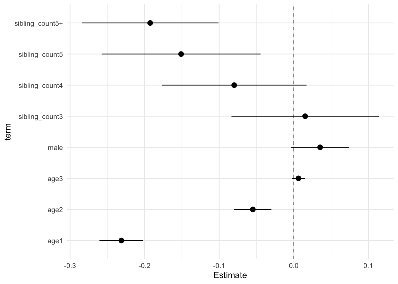
Add Birth Order Linear
Model Summary
model_genes_m2 <- with(data_used, lmer(outcome ~ birth_order + poly(age, degree = 3, raw = T)+ male + sibling_count +
                                         (1 | mother_pidlink), REML = FALSE))
x = mitml::testEstimates(model_genes_m2, var.comp = T)

y = as_tibble(x$estimates, rownames = "id")

y = y %>%
  mutate(CI_low = Estimate - 2.576 * Std.Error,
         CI_high = Estimate + 2.576 * Std.Error) %>%
  select(CI_low, CI_high)
CI_low = y$CI_low
CI_high = y$CI_high


x$estimates = cbind(x$estimates[,1:2], CI_low, CI_high, x$estimates[,3:7])
x
##
## Call:
##
## mitml::testEstimates(model = model_genes_m2, var.comp = T)
##
## Final parameter estimates and inferences obtained from 50 imputed data sets.
##
## Estimate Std.Error CI_low CI_high t.value df P(>|t|) RIV FMI
## (Intercept) 0.121 0.030 0.044 0.199 4.046 683.276 0.000 0.366 0.270
## birth_order -0.000 0.006 -0.015 0.015 -0.029 289.041 0.977 0.700 0.416
## poly(age, degree = 3, raw = T)1 -0.231 0.012 -0.261 -0.201 -19.964 3315.106 0.000 0.138 0.122
## poly(age, degree = 3, raw = T)2 -0.055 0.010 -0.080 -0.030 -5.681 2336.939 0.000 0.169 0.146
## poly(age, degree = 3, raw = T)3 0.006 0.004 -0.003 0.015 1.815 1243.079 0.070 0.248 0.200
## male 0.035 0.015 -0.004 0.074 2.342 2711.683 0.019 0.155 0.135
## sibling_count3 0.015 0.039 -0.084 0.115 0.398 300.459 0.691 0.677 0.408
## sibling_count4 -0.080 0.038 -0.178 0.019 -2.085 398.648 0.038 0.540 0.354
## sibling_count5 -0.151 0.042 -0.260 -0.042 -3.558 345.278 0.000 0.604 0.380
## sibling_count5+ -0.192 0.040 -0.296 -0.089 -4.791 316.216 0.000 0.649 0.397
##
## Estimate
## Intercept~~Intercept|mother_pidlink 0.312
## Residual~~Residual 0.616
## ICC|mother_pidlink 0.336
##
## Unadjusted hypothesis test as appropriate in larger samples.x$estimates %>%
as.data.frame() %>%
tibble::rownames_to_column("term") %>%
filter(term != "(Intercept)") %>%
mutate(term = str_replace_all(term, "poly\\(", "")) %>%
mutate(term = str_replace_all(term, ", degree = 3, raw = T\\)", "")) %>%
ggplot(aes(x= term, y = Estimate, ymin = CI_low, ymax = CI_high)) +
geom_hline(yintercept = 0, linetype = "dashed", alpha = 0.5) +
geom_pointrange() +
coord_flip() +
theme_minimal()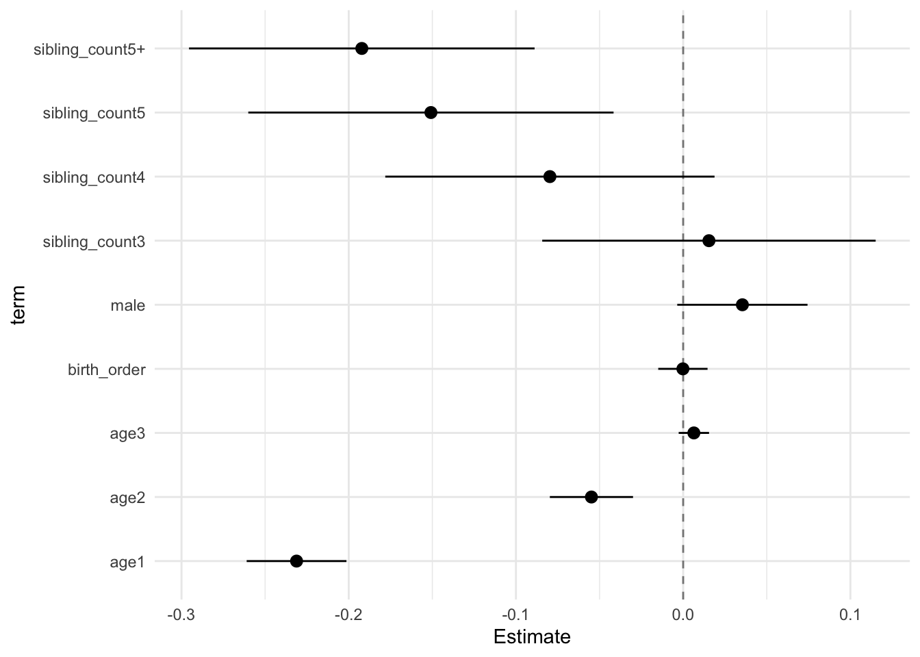
Add Birth Order Factor
Model Summary
model_genes_m3 <- with(data_used, lmer(outcome ~ birth_order_nonlinear + poly(age, degree = 3, raw = T)+ male + sibling_count +
                                         (1 | mother_pidlink), REML = FALSE))
x = mitml::testEstimates(model_genes_m3, var.comp = T)

y = as_tibble(x$estimates, rownames = "id")

y = y %>%
  mutate(CI_low = Estimate - 2.576 * Std.Error,
         CI_high = Estimate + 2.576 * Std.Error) %>%
  select(CI_low, CI_high)
CI_low = y$CI_low
CI_high = y$CI_high


x$estimates = cbind(x$estimates[,1:2], CI_low, CI_high, x$estimates[,3:7])
x
##
## Call:
##
## mitml::testEstimates(model = model_genes_m3, var.comp = T)
##
## Final parameter estimates and inferences obtained from 50 imputed data sets.
##
## Estimate Std.Error CI_low CI_high t.value df P(>|t|) RIV FMI
## (Intercept) 0.117 0.031 0.038 0.195 3.819 593.014 0.000 0.403 0.290
## birth_order_nonlinear2 0.015 0.024 -0.047 0.077 0.617 251.526 0.538 0.790 0.446
## birth_order_nonlinear3 0.018 0.027 -0.052 0.089 0.661 368.639 0.509 0.574 0.368
## birth_order_nonlinear4 0.006 0.034 -0.083 0.095 0.168 299.325 0.867 0.680 0.409
## birth_order_nonlinear5 0.022 0.044 -0.092 0.136 0.507 303.532 0.613 0.672 0.406
## birth_order_nonlinear5+ -0.006 0.041 -0.113 0.101 -0.148 320.673 0.882 0.642 0.395
## poly(age, degree = 3, raw = T)1 -0.231 0.012 -0.261 -0.201 -19.977 3351.285 0.000 0.138 0.121
## poly(age, degree = 3, raw = T)2 -0.055 0.010 -0.080 -0.030 -5.713 2363.845 0.000 0.168 0.145
## poly(age, degree = 3, raw = T)3 0.006 0.004 -0.003 0.016 1.840 1264.896 0.066 0.245 0.198
## male 0.035 0.015 -0.004 0.074 2.338 2703.547 0.019 0.156 0.135
## sibling_count3 0.012 0.039 -0.090 0.113 0.295 289.968 0.768 0.698 0.415
## sibling_count4 -0.083 0.039 -0.184 0.018 -2.123 381.296 0.034 0.559 0.362
## sibling_count5 -0.157 0.043 -0.268 -0.045 -3.629 345.170 0.000 0.605 0.380
## sibling_count5+ -0.194 0.040 -0.298 -0.089 -4.786 310.613 0.000 0.659 0.401
##
## Estimate
## Intercept~~Intercept|mother_pidlink 0.312
## Residual~~Residual 0.616
## ICC|mother_pidlink 0.336
##
## Unadjusted hypothesis test as appropriate in larger samples.x$estimates %>%
as.data.frame() %>%
tibble::rownames_to_column("term") %>%
filter(term != "(Intercept)") %>%
mutate(term = str_replace_all(term, "poly\\(", "")) %>%
mutate(term = str_replace_all(term, ", degree = 3, raw = T\\)", "")) %>%
ggplot(aes(x= term, y = Estimate, ymin = CI_low, ymax = CI_high)) +
geom_hline(yintercept = 0, linetype = "dashed", alpha = 0.5) +
geom_pointrange() +
coord_flip() +
theme_minimal()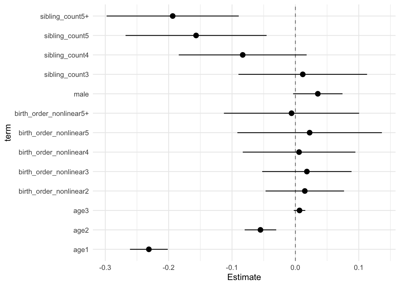
Add Interaction
Model Summary
model_genes_m4 <- with(data_used, lmer(outcome ~ count_birth_order + poly(age, degree = 3, raw = T)+ male  +
                                         (1 | mother_pidlink), REML = FALSE))
x = mitml::testEstimates(model_genes_m4, var.comp = T)

y = as_tibble(x$estimates, rownames = "id")

y = y %>%
  mutate(CI_low = Estimate - 2.576 * Std.Error,
         CI_high = Estimate + 2.576 * Std.Error) %>%
  select(CI_low, CI_high)
CI_low = y$CI_low
CI_high = y$CI_high


x$estimates = cbind(x$estimates[,1:2], CI_low, CI_high, x$estimates[,3:7])
x
##
## Call:
##
## mitml::testEstimates(model = model_genes_m4, var.comp = T)
##
## Final parameter estimates and inferences obtained from 50 imputed data sets.
##
## Estimate Std.Error CI_low CI_high t.value df P(>|t|) RIV FMI
## (Intercept) 0.123 0.033 0.036 0.209 3.662 567.433 0.000 0.416 0.296
## count_birth_order2/2 -0.003 0.046 -0.121 0.116 -0.061 478.384 0.951 0.471 0.323
## count_birth_order1/3 0.005 0.047 -0.116 0.126 0.110 310.826 0.913 0.658 0.401
## count_birth_order2/3 0.040 0.051 -0.091 0.172 0.794 343.742 0.428 0.607 0.381
## count_birth_order3/3 0.000 0.052 -0.134 0.134 0.006 439.671 0.995 0.501 0.337
## count_birth_order1/4 -0.103 0.051 -0.235 0.029 -2.013 286.428 0.045 0.705 0.418
## count_birth_order2/4 -0.063 0.053 -0.200 0.074 -1.190 346.449 0.235 0.603 0.380
## count_birth_order3/4 -0.057 0.055 -0.199 0.086 -1.025 521.512 0.306 0.442 0.309
## count_birth_order4/4 -0.086 0.056 -0.230 0.059 -1.529 388.954 0.127 0.550 0.358
## count_birth_order1/5 -0.156 0.058 -0.304 -0.007 -2.696 281.130 0.007 0.717 0.422
## count_birth_order2/5 -0.147 0.064 -0.313 0.018 -2.289 276.475 0.023 0.727 0.425
## count_birth_order3/5 -0.150 0.064 -0.314 0.015 -2.348 470.637 0.019 0.476 0.326
## count_birth_order4/5 -0.149 0.068 -0.325 0.027 -2.186 489.888 0.029 0.463 0.319
## count_birth_order5/5 -0.156 0.070 -0.337 0.025 -2.217 257.450 0.028 0.774 0.441
## count_birth_order1/5+ -0.198 0.053 -0.336 -0.060 -3.705 241.451 0.000 0.820 0.455
## count_birth_order2/5+ -0.209 0.054 -0.347 -0.070 -3.883 342.730 0.000 0.608 0.382
## count_birth_order3/5+ -0.163 0.060 -0.318 -0.007 -2.696 260.862 0.007 0.765 0.438
## count_birth_order4/5+ -0.195 0.057 -0.342 -0.048 -3.418 532.264 0.001 0.436 0.306
## count_birth_order5/5+ -0.162 0.062 -0.321 -0.003 -2.627 467.388 0.009 0.479 0.327
## count_birth_order5+/5+ -0.205 0.046 -0.323 -0.087 -4.480 594.011 0.000 0.403 0.290
## poly(age, degree = 3, raw = T)1 -0.231 0.012 -0.261 -0.201 -19.979 3402.879 0.000 0.136 0.121
## poly(age, degree = 3, raw = T)2 -0.055 0.010 -0.080 -0.030 -5.680 2217.049 0.000 0.175 0.149
## poly(age, degree = 3, raw = T)3 0.006 0.004 -0.003 0.016 1.836 1229.337 0.067 0.249 0.201
## male 0.035 0.015 -0.004 0.074 2.337 2736.574 0.020 0.154 0.134
##
## Estimate
## Intercept~~Intercept|mother_pidlink 0.312
## Residual~~Residual 0.616
## ICC|mother_pidlink 0.336
##
## Unadjusted hypothesis test as appropriate in larger samples.x$estimates %>%
as.data.frame() %>%
tibble::rownames_to_column("term") %>%
filter(term != "(Intercept)") %>%
mutate(term = str_replace_all(term, "poly\\(", "")) %>%
mutate(term = str_replace_all(term, ", degree = 3, raw = T\\)", "")) %>%
ggplot(aes(x= term, y = Estimate, ymin = CI_low, ymax = CI_high)) +
geom_hline(yintercept = 0, linetype = "dashed", alpha = 0.5) +
geom_pointrange() +
coord_flip() +
theme_minimal()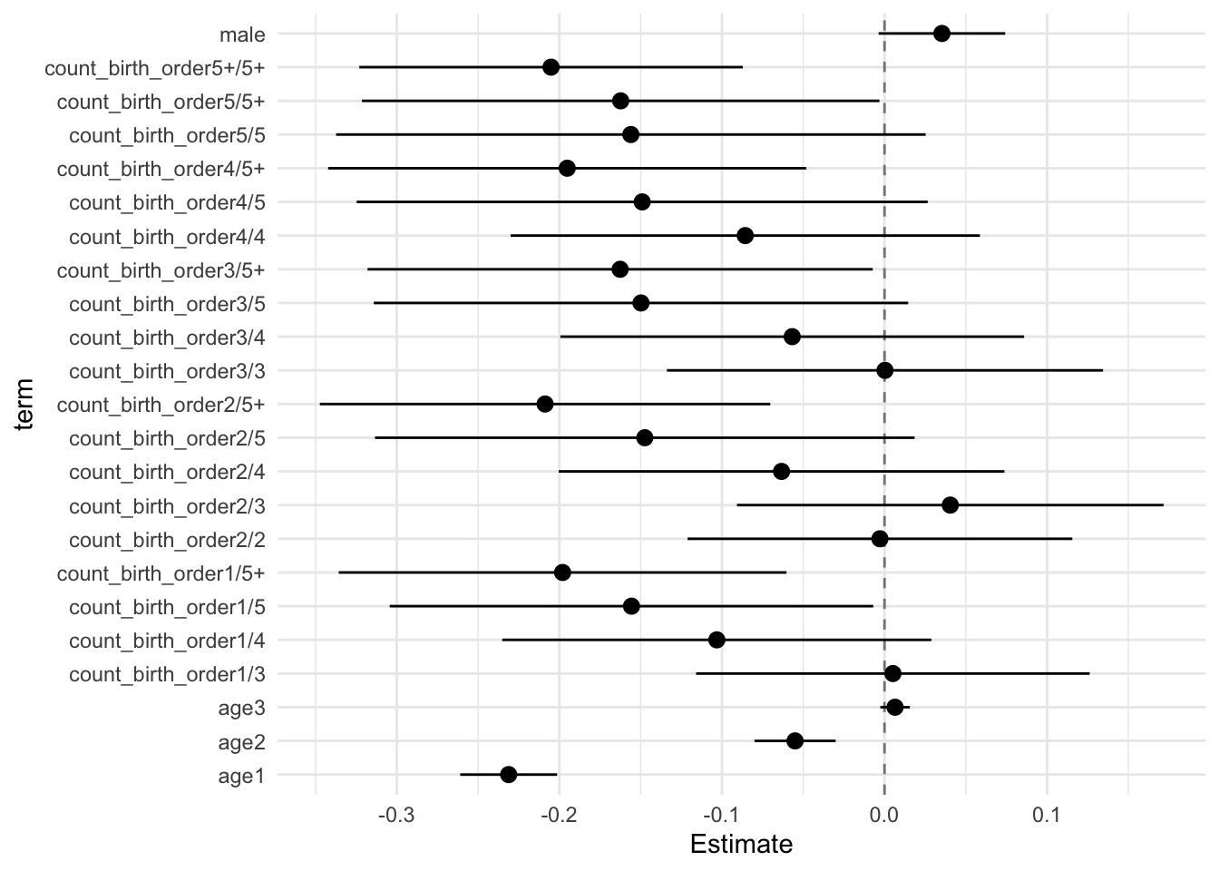
Model Comparison
anova(model_genes_m1, model_genes_m2, model_genes_m3, model_genes_m4)##
## Call:
##
## anova.mitml.result(object = model_genes_m1, model_genes_m2, model_genes_m3,
## model_genes_m4)
##
## Model comparison calculated from 50 imputed data sets.
## Combination method: D3
##
## Model 1: outcome~count_birth_order+poly(age,degree=3,raw=T)+male+(1|mother_pidlink)
## Model 2: outcome~birth_order_nonlinear+poly(age,degree=3,raw=T)+male+sibling_count+(1|mother_pidlink)
## Model 3: outcome~birth_order+poly(age,degree=3,raw=T)+male+sibling_count+(1|mother_pidlink)
## Model 4: outcome~poly(age,degree=3,raw=T)+male+sibling_count+(1|mother_pidlink)
##
## F.value df1 df2 P(>F) RIV
## 1 vs 2: 0.188 10 3030.462 0.997 0.666
## 2 vs 3: 0.234 4 1271.782 0.919 0.631
## 3 vs 4: 0.001 1 257.226 0.979 0.699g-factor 2015 young
# Specify your outcome
data_used = data_used %>% mutate(outcome = g_factor_2015_young)
data_used_plots <- data_used[[1]]

compare_birthorder_imputed(data_used = data_used)
Parental full sibling order
Basic Model
# with.mitml.list <- function (data, expr, ...)
# {
#     expr <- substitute(expr)
#     parent <- parent.frame()
#     out <- parallel::mclapply(data, function(x) eval(expr, x, parent))
#     class(out) <- c("mitml.result", "list")
#     out
# }
Model Summary
data_used = data_used %>%
  mutate(sibling_count = sibling_count_genes_factor,
         birth_order_nonlinear = birthorder_genes_factor,
         birth_order = birthorder_genes,
         count_birth_order = count_birthorder_genes)

data_used_plots = data_used[[1]]

model_genes_m1 <- with(data_used, lmer(outcome ~ poly(age, degree = 3, raw = T)+ male + sibling_count + (1 | mother_pidlink), REML = FALSE))
x = mitml::testEstimates(model_genes_m1, var.comp = T)

y = as_tibble(x$estimates, rownames = "id")

y = y %>%
  mutate(CI_low = Estimate - 2.576 * Std.Error,
         CI_high = Estimate + 2.576 * Std.Error) %>%
  select(CI_low, CI_high)
CI_low = y$CI_low
CI_high = y$CI_high


x$estimates = cbind(x$estimates[,1:2], CI_low, CI_high, x$estimates[,3:7])
x
##
## Call:
##
## mitml::testEstimates(model = model_genes_m1, var.comp = T)
##
## Final parameter estimates and inferences obtained from 50 imputed data sets.
##
## Estimate Std.Error CI_low CI_high t.value df P(>|t|) RIV FMI
## (Intercept) -0.009 0.090 -0.241 0.223 -0.096 57.313 0.924 12.270 0.927
## poly(age, degree = 3, raw = T)1 -0.098 0.083 -0.312 0.115 -1.186 50.660 0.241 59.520 0.984
## poly(age, degree = 3, raw = T)2 0.073 0.066 -0.097 0.243 1.112 50.841 0.272 53.730 0.982
## poly(age, degree = 3, raw = T)3 0.023 0.030 -0.054 0.099 0.771 50.119 0.445 88.109 0.989
## male -0.027 0.018 -0.074 0.020 -1.469 306.246 0.143 0.667 0.404
## sibling_count3 0.021 0.037 -0.073 0.115 0.580 367.095 0.562 0.576 0.369
## sibling_count4 -0.058 0.038 -0.155 0.039 -1.547 355.762 0.123 0.590 0.375
## sibling_count5 -0.107 0.040 -0.210 -0.003 -2.656 375.696 0.008 0.565 0.365
## sibling_count5+ -0.152 0.037 -0.247 -0.058 -4.154 307.021 0.000 0.665 0.403
##
## Estimate
## Intercept~~Intercept|mother_pidlink 0.268
## Residual~~Residual 0.641
## ICC|mother_pidlink 0.295
##
## Unadjusted hypothesis test as appropriate in larger samples.x$estimates %>%
as.data.frame() %>%
tibble::rownames_to_column("term") %>%
filter(term != "(Intercept)") %>%
mutate(term = str_replace_all(term, "poly\\(", "")) %>%
mutate(term = str_replace_all(term, ", degree = 3, raw = T\\)", "")) %>%
ggplot(aes(x= term, y = Estimate, ymin = CI_low, ymax = CI_high)) +
geom_hline(yintercept = 0, linetype = "dashed", alpha = 0.5) +
geom_pointrange() +
coord_flip() +
theme_minimal()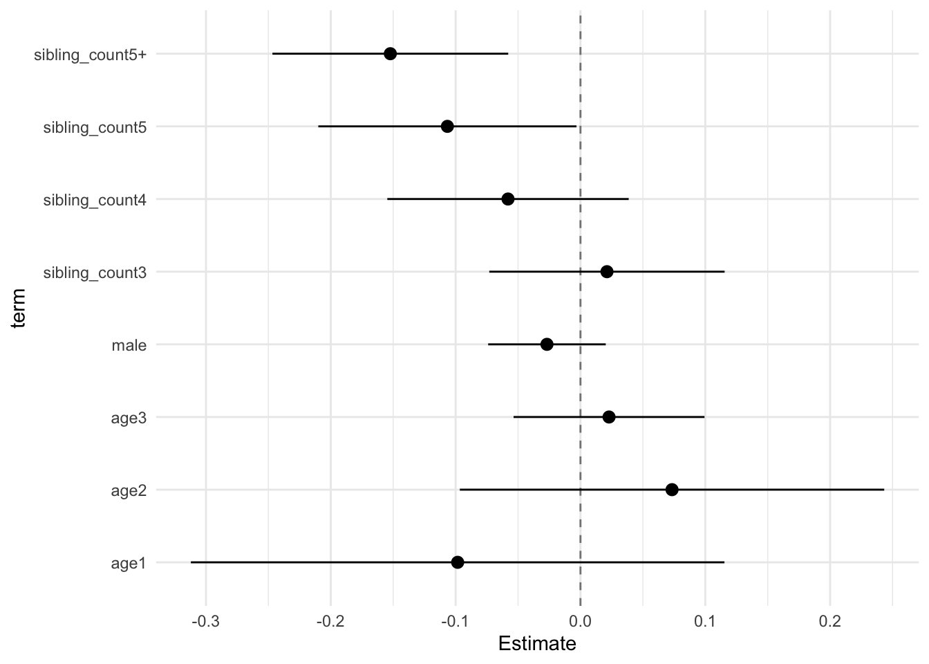
Add Birth Order Linear
Model Summary
model_genes_m2 <- with(data_used, lmer(outcome ~ birth_order + poly(age, degree = 3, raw = T)+ male + sibling_count +
                                         (1 | mother_pidlink), REML = FALSE))
x = mitml::testEstimates(model_genes_m2, var.comp = T)

y = as_tibble(x$estimates, rownames = "id")

y = y %>%
  mutate(CI_low = Estimate - 2.576 * Std.Error,
         CI_high = Estimate + 2.576 * Std.Error) %>%
  select(CI_low, CI_high)
CI_low = y$CI_low
CI_high = y$CI_high


x$estimates = cbind(x$estimates[,1:2], CI_low, CI_high, x$estimates[,3:7])
x
##
## Call:
##
## mitml::testEstimates(model = model_genes_m2, var.comp = T)
##
## Final parameter estimates and inferences obtained from 50 imputed data sets.
##
## Estimate Std.Error CI_low CI_high t.value df P(>|t|) RIV FMI
## (Intercept) -0.006 0.091 -0.240 0.227 -0.071 57.641 0.944 11.821 0.925
## birth_order -0.002 0.006 -0.016 0.013 -0.303 297.644 0.762 0.683 0.410
## poly(age, degree = 3, raw = T)1 -0.099 0.083 -0.314 0.116 -1.187 50.672 0.241 59.092 0.984
## poly(age, degree = 3, raw = T)2 0.073 0.066 -0.097 0.243 1.111 50.841 0.272 53.740 0.982
## poly(age, degree = 3, raw = T)3 0.023 0.030 -0.054 0.099 0.772 50.119 0.444 88.083 0.989
## male -0.027 0.018 -0.074 0.020 -1.470 306.714 0.143 0.666 0.404
## sibling_count3 0.022 0.037 -0.072 0.116 0.602 373.711 0.547 0.568 0.365
## sibling_count4 -0.056 0.038 -0.154 0.041 -1.485 356.211 0.138 0.590 0.374
## sibling_count5 -0.104 0.041 -0.210 0.002 -2.534 360.716 0.012 0.584 0.372
## sibling_count5+ -0.148 0.040 -0.252 -0.044 -3.655 265.894 0.000 0.752 0.434
##
## Estimate
## Intercept~~Intercept|mother_pidlink 0.268
## Residual~~Residual 0.641
## ICC|mother_pidlink 0.295
##
## Unadjusted hypothesis test as appropriate in larger samples.x$estimates %>%
as.data.frame() %>%
tibble::rownames_to_column("term") %>%
filter(term != "(Intercept)") %>%
mutate(term = str_replace_all(term, "poly\\(", "")) %>%
mutate(term = str_replace_all(term, ", degree = 3, raw = T\\)", "")) %>%
ggplot(aes(x= term, y = Estimate, ymin = CI_low, ymax = CI_high)) +
geom_hline(yintercept = 0, linetype = "dashed", alpha = 0.5) +
geom_pointrange() +
coord_flip() +
theme_minimal()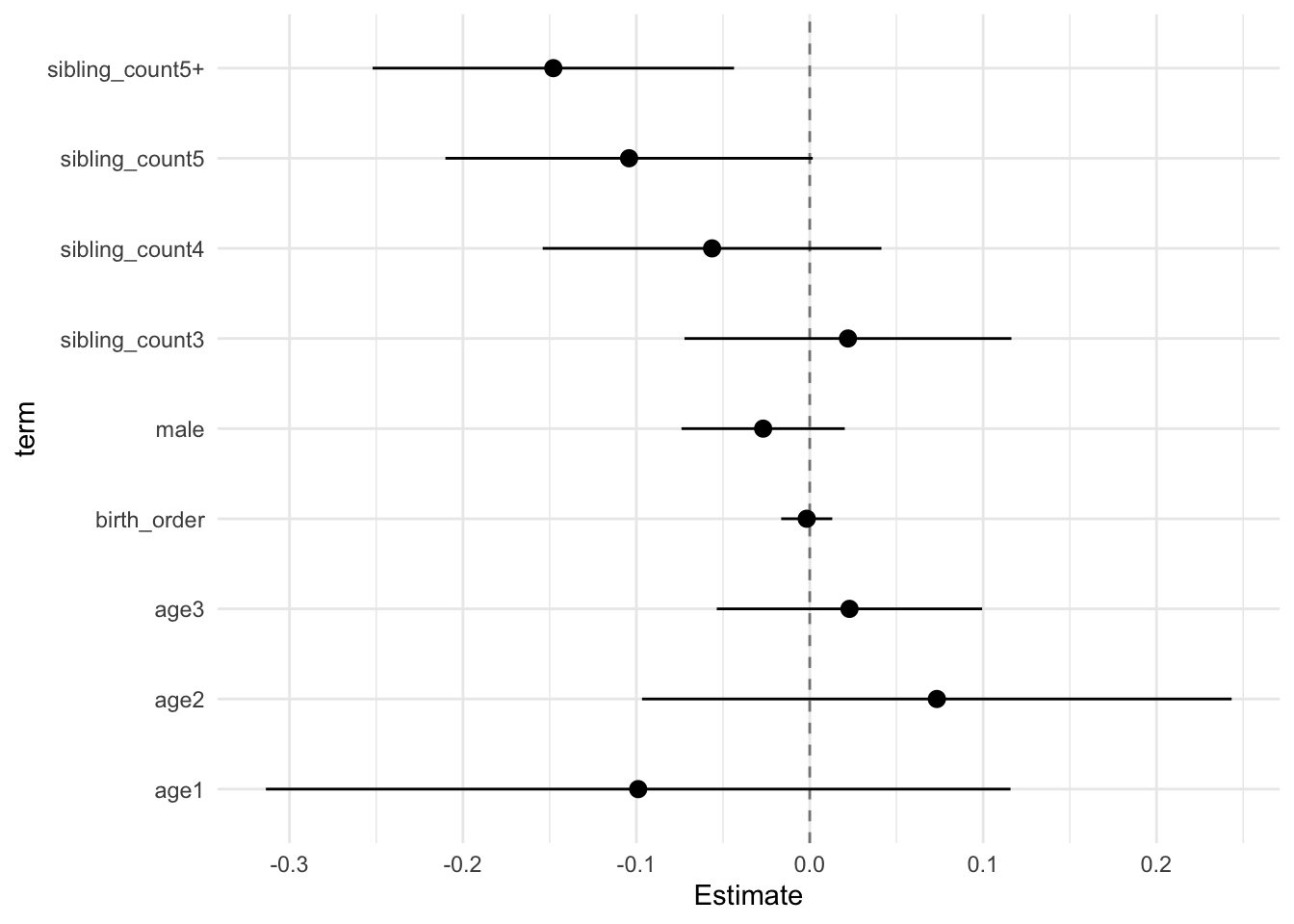
Add Birth Order Factor
Model Summary
model_genes_m3 <- with(data_used, lmer(outcome ~ birth_order_nonlinear + poly(age, degree = 3, raw = T)+ male + sibling_count +
                                         (1 | mother_pidlink), REML = FALSE))
x = mitml::testEstimates(model_genes_m3, var.comp = T)

y = as_tibble(x$estimates, rownames = "id")

y = y %>%
  mutate(CI_low = Estimate - 2.576 * Std.Error,
         CI_high = Estimate + 2.576 * Std.Error) %>%
  select(CI_low, CI_high)
CI_low = y$CI_low
CI_high = y$CI_high


x$estimates = cbind(x$estimates[,1:2], CI_low, CI_high, x$estimates[,3:7])
x
##
## Call:
##
## mitml::testEstimates(model = model_genes_m3, var.comp = T)
##
## Final parameter estimates and inferences obtained from 50 imputed data sets.
##
## Estimate Std.Error CI_low CI_high t.value df P(>|t|) RIV FMI
## (Intercept) -0.011 0.091 -0.245 0.224 -0.117 57.631 0.907 11.835 0.925
## birth_order_nonlinear2 0.007 0.024 -0.055 0.068 0.283 268.161 0.777 0.747 0.432
## birth_order_nonlinear3 0.025 0.030 -0.052 0.102 0.835 232.455 0.405 0.849 0.464
## birth_order_nonlinear4 0.014 0.035 -0.077 0.105 0.394 274.813 0.694 0.731 0.426
## birth_order_nonlinear5 -0.003 0.044 -0.117 0.111 -0.067 312.006 0.947 0.656 0.400
## birth_order_nonlinear5+ -0.001 0.045 -0.116 0.113 -0.029 224.075 0.977 0.878 0.472
## poly(age, degree = 3, raw = T)1 -0.098 0.083 -0.313 0.116 -1.182 50.675 0.243 59.006 0.984
## poly(age, degree = 3, raw = T)2 0.073 0.066 -0.097 0.243 1.108 50.842 0.273 53.693 0.982
## poly(age, degree = 3, raw = T)3 0.023 0.030 -0.054 0.099 0.773 50.120 0.443 87.988 0.989
## male -0.027 0.018 -0.074 0.020 -1.467 302.611 0.144 0.673 0.406
## sibling_count3 0.015 0.037 -0.080 0.111 0.416 359.478 0.678 0.585 0.373
## sibling_count4 -0.065 0.039 -0.166 0.037 -1.645 314.799 0.101 0.652 0.398
## sibling_count5 -0.111 0.043 -0.222 0.000 -2.575 299.372 0.011 0.679 0.409
## sibling_count5+ -0.155 0.041 -0.261 -0.050 -3.808 261.603 0.000 0.763 0.437
##
## Estimate
## Intercept~~Intercept|mother_pidlink 0.268
## Residual~~Residual 0.641
## ICC|mother_pidlink 0.295
##
## Unadjusted hypothesis test as appropriate in larger samples.x$estimates %>%
as.data.frame() %>%
tibble::rownames_to_column("term") %>%
filter(term != "(Intercept)") %>%
mutate(term = str_replace_all(term, "poly\\(", "")) %>%
mutate(term = str_replace_all(term, ", degree = 3, raw = T\\)", "")) %>%
ggplot(aes(x= term, y = Estimate, ymin = CI_low, ymax = CI_high)) +
geom_hline(yintercept = 0, linetype = "dashed", alpha = 0.5) +
geom_pointrange() +
coord_flip() +
theme_minimal()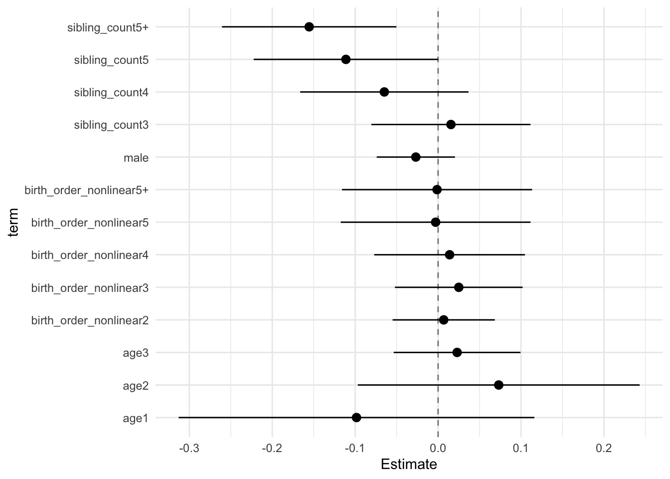
Add Interaction
Model Summary
model_genes_m4 <- with(data_used, lmer(outcome ~ count_birth_order + poly(age, degree = 3, raw = T)+ male  +
                                         (1 | mother_pidlink), REML = FALSE))
x = mitml::testEstimates(model_genes_m4, var.comp = T)

y = as_tibble(x$estimates, rownames = "id")

y = y %>%
  mutate(CI_low = Estimate - 2.576 * Std.Error,
         CI_high = Estimate + 2.576 * Std.Error) %>%
  select(CI_low, CI_high)
CI_low = y$CI_low
CI_high = y$CI_high


x$estimates = cbind(x$estimates[,1:2], CI_low, CI_high, x$estimates[,3:7])
x
##
## Call:
##
## mitml::testEstimates(model = model_genes_m4, var.comp = T)
##
## Final parameter estimates and inferences obtained from 50 imputed data sets.
##
## Estimate Std.Error CI_low CI_high t.value df P(>|t|) RIV FMI
## (Intercept) -0.002 0.091 -0.237 0.233 -0.021 59.610 0.983 9.712 0.910
## count_birth_order2/2 -0.019 0.048 -0.144 0.105 -0.398 339.777 0.691 0.612 0.383
## count_birth_order1/3 0.008 0.049 -0.117 0.133 0.173 244.916 0.863 0.809 0.452
## count_birth_order2/3 0.035 0.049 -0.091 0.162 0.720 413.250 0.472 0.525 0.347
## count_birth_order3/3 0.001 0.054 -0.137 0.140 0.025 337.237 0.980 0.616 0.385
## count_birth_order1/4 -0.086 0.052 -0.219 0.047 -1.658 258.189 0.099 0.772 0.440
## count_birth_order2/4 -0.073 0.054 -0.212 0.066 -1.346 301.042 0.179 0.676 0.407
## count_birth_order3/4 -0.023 0.058 -0.173 0.128 -0.390 334.329 0.697 0.620 0.386
## count_birth_order4/4 -0.055 0.057 -0.201 0.092 -0.965 337.450 0.335 0.616 0.385
## count_birth_order1/5 -0.118 0.057 -0.265 0.028 -2.080 288.207 0.038 0.702 0.416
## count_birth_order2/5 -0.112 0.067 -0.284 0.060 -1.681 225.240 0.094 0.874 0.471
## count_birth_order3/5 -0.085 0.063 -0.249 0.078 -1.342 475.144 0.180 0.473 0.324
## count_birth_order4/5 -0.125 0.069 -0.303 0.052 -1.820 438.075 0.069 0.503 0.337
## count_birth_order5/5 -0.123 0.069 -0.302 0.055 -1.778 274.971 0.076 0.731 0.426
## count_birth_order1/5+ -0.168 0.055 -0.309 -0.027 -3.078 208.390 0.002 0.941 0.490
## count_birth_order2/5+ -0.162 0.053 -0.297 -0.026 -3.080 382.425 0.002 0.558 0.361
## count_birth_order3/5+ -0.134 0.063 -0.297 0.029 -2.112 205.071 0.036 0.956 0.494
## count_birth_order4/5+ -0.143 0.061 -0.300 0.013 -2.359 325.199 0.019 0.634 0.392
## count_birth_order5/5+ -0.167 0.068 -0.342 0.007 -2.470 254.860 0.014 0.781 0.443
## count_birth_order5+/5+ -0.165 0.050 -0.293 -0.038 -3.338 301.147 0.001 0.676 0.407
## poly(age, degree = 3, raw = T)1 -0.098 0.083 -0.313 0.116 -1.182 50.680 0.243 58.824 0.984
## poly(age, degree = 3, raw = T)2 0.073 0.066 -0.097 0.243 1.109 50.843 0.273 53.680 0.982
## poly(age, degree = 3, raw = T)3 0.023 0.030 -0.054 0.099 0.772 50.120 0.444 88.008 0.989
## male -0.027 0.018 -0.074 0.020 -1.461 305.641 0.145 0.668 0.404
##
## Estimate
## Intercept~~Intercept|mother_pidlink 0.268
## Residual~~Residual 0.641
## ICC|mother_pidlink 0.295
##
## Unadjusted hypothesis test as appropriate in larger samples.x$estimates %>%
as.data.frame() %>%
tibble::rownames_to_column("term") %>%
filter(term != "(Intercept)") %>%
mutate(term = str_replace_all(term, "poly\\(", "")) %>%
mutate(term = str_replace_all(term, ", degree = 3, raw = T\\)", "")) %>%
ggplot(aes(x= term, y = Estimate, ymin = CI_low, ymax = CI_high)) +
geom_hline(yintercept = 0, linetype = "dashed", alpha = 0.5) +
geom_pointrange() +
coord_flip() +
theme_minimal()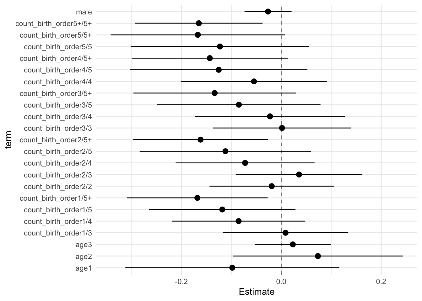
Model Comparison
anova(model_genes_m1, model_genes_m2, model_genes_m3, model_genes_m4)##
## Call:
##
## anova.mitml.result(object = model_genes_m1, model_genes_m2, model_genes_m3,
## model_genes_m4)
##
## Model comparison calculated from 50 imputed data sets.
## Combination method: D3
##
## Model 1: outcome~count_birth_order+poly(age,degree=3,raw=T)+male+(1|mother_pidlink)
## Model 2: outcome~birth_order_nonlinear+poly(age,degree=3,raw=T)+male+sibling_count+(1|mother_pidlink)
## Model 3: outcome~birth_order+poly(age,degree=3,raw=T)+male+sibling_count+(1|mother_pidlink)
## Model 4: outcome~poly(age,degree=3,raw=T)+male+sibling_count+(1|mother_pidlink)
##
## F.value df1 df2 P(>F) RIV
## 1 vs 2: 0.131 10 2167.699 0.999 0.897
## 2 vs 3: 0.147 4 904.369 0.964 0.849
## 3 vs 4: 0.094 1 263.879 0.760 0.684Personality
Extraversion
# Specify your outcome
data_used = data_used %>% mutate(outcome = big5_ext)
data_used_plots <- data_used[[1]]

compare_birthorder_imputed(data_used = data_used)
Parental full sibling order
Basic Model
# with.mitml.list <- function (data, expr, ...)
# {
#     expr <- substitute(expr)
#     parent <- parent.frame()
#     out <- parallel::mclapply(data, function(x) eval(expr, x, parent))
#     class(out) <- c("mitml.result", "list")
#     out
# }
Model Summary
data_used = data_used %>%
  mutate(sibling_count = sibling_count_genes_factor,
         birth_order_nonlinear = birthorder_genes_factor,
         birth_order = birthorder_genes,
         count_birth_order = count_birthorder_genes)

data_used_plots = data_used[[1]]

model_genes_m1 <- with(data_used, lmer(outcome ~ poly(age, degree = 3, raw = T)+ male + sibling_count + (1 | mother_pidlink), REML = FALSE))
x = mitml::testEstimates(model_genes_m1, var.comp = T)

y = as_tibble(x$estimates, rownames = "id")

y = y %>%
  mutate(CI_low = Estimate - 2.576 * Std.Error,
         CI_high = Estimate + 2.576 * Std.Error) %>%
  select(CI_low, CI_high)
CI_low = y$CI_low
CI_high = y$CI_high


x$estimates = cbind(x$estimates[,1:2], CI_low, CI_high, x$estimates[,3:7])
x
##
## Call:
##
## mitml::testEstimates(model = model_genes_m1, var.comp = T)
##
## Final parameter estimates and inferences obtained from 50 imputed data sets.
##
## Estimate Std.Error CI_low CI_high t.value df P(>|t|) RIV FMI
## (Intercept) 0.138 0.029 0.065 0.212 4.854 714.856 0.000 0.355 0.264
## poly(age, degree = 3, raw = T)1 -0.000 0.011 -0.029 0.029 -0.016 6508.682 0.987 0.095 0.087
## poly(age, degree = 3, raw = T)2 0.018 0.010 -0.007 0.044 1.836 3625.354 0.066 0.132 0.117
## poly(age, degree = 3, raw = T)3 -0.011 0.003 -0.019 -0.002 -3.131 10116.541 0.002 0.075 0.070
## male -0.225 0.017 -0.269 -0.182 -13.332 2332.303 0.000 0.170 0.146
## sibling_count3 -0.021 0.032 -0.105 0.063 -0.644 709.867 0.520 0.356 0.265
## sibling_count4 -0.051 0.035 -0.141 0.040 -1.438 373.512 0.151 0.568 0.366
## sibling_count5 -0.049 0.037 -0.145 0.047 -1.321 400.678 0.187 0.538 0.353
## sibling_count5+ -0.056 0.032 -0.138 0.025 -1.782 569.796 0.075 0.415 0.296
##
## Estimate
## Intercept~~Intercept|mother_pidlink 0.059
## Residual~~Residual 0.926
## ICC|mother_pidlink 0.060
##
## Unadjusted hypothesis test as appropriate in larger samples.x$estimates %>%
as.data.frame() %>%
tibble::rownames_to_column("term") %>%
filter(term != "(Intercept)") %>%
mutate(term = str_replace_all(term, "poly\\(", "")) %>%
mutate(term = str_replace_all(term, ", degree = 3, raw = T\\)", "")) %>%
ggplot(aes(x= term, y = Estimate, ymin = CI_low, ymax = CI_high)) +
geom_hline(yintercept = 0, linetype = "dashed", alpha = 0.5) +
geom_pointrange() +
coord_flip() +
theme_minimal()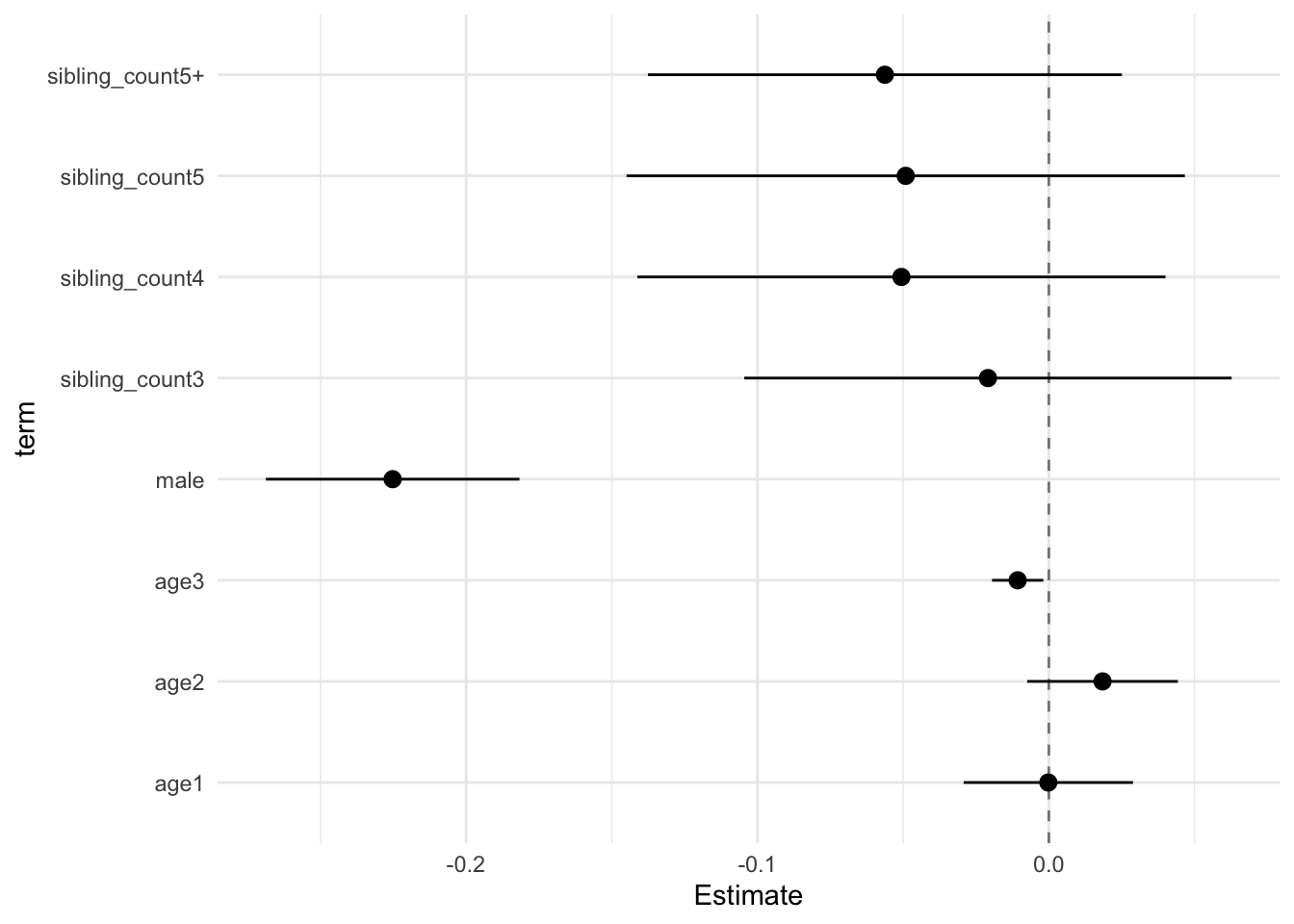
Add Birth Order Linear
Model Summary
model_genes_m2 <- with(data_used, lmer(outcome ~ birth_order + poly(age, degree = 3, raw = T)+ male + sibling_count +
                                         (1 | mother_pidlink), REML = FALSE))
x = mitml::testEstimates(model_genes_m2, var.comp = T)

y = as_tibble(x$estimates, rownames = "id")

y = y %>%
  mutate(CI_low = Estimate - 2.576 * Std.Error,
         CI_high = Estimate + 2.576 * Std.Error) %>%
  select(CI_low, CI_high)
CI_low = y$CI_low
CI_high = y$CI_high


x$estimates = cbind(x$estimates[,1:2], CI_low, CI_high, x$estimates[,3:7])
x
##
## Call:
##
## mitml::testEstimates(model = model_genes_m2, var.comp = T)
##
## Final parameter estimates and inferences obtained from 50 imputed data sets.
##
## Estimate Std.Error CI_low CI_high t.value df P(>|t|) RIV FMI
## (Intercept) 0.128 0.029 0.054 0.202 4.434 912.177 0.000 0.302 0.233
## birth_order 0.008 0.006 -0.008 0.023 1.310 353.151 0.191 0.594 0.376
## poly(age, degree = 3, raw = T)1 0.001 0.011 -0.028 0.031 0.120 5920.337 0.904 0.100 0.091
## poly(age, degree = 3, raw = T)2 0.019 0.010 -0.007 0.045 1.877 3594.521 0.061 0.132 0.117
## poly(age, degree = 3, raw = T)3 -0.011 0.003 -0.020 -0.002 -3.179 9930.217 0.001 0.076 0.070
## male -0.225 0.017 -0.269 -0.182 -13.339 2370.631 0.000 0.168 0.144
## sibling_count3 -0.024 0.033 -0.109 0.060 -0.747 671.102 0.455 0.370 0.272
## sibling_count4 -0.058 0.036 -0.151 0.035 -1.602 339.181 0.110 0.613 0.384
## sibling_count5 -0.059 0.038 -0.158 0.039 -1.554 379.174 0.121 0.561 0.363
## sibling_count5+ -0.076 0.037 -0.170 0.018 -2.078 363.955 0.038 0.580 0.370
##
## Estimate
## Intercept~~Intercept|mother_pidlink 0.059
## Residual~~Residual 0.926
## ICC|mother_pidlink 0.060
##
## Unadjusted hypothesis test as appropriate in larger samples.x$estimates %>%
as.data.frame() %>%
tibble::rownames_to_column("term") %>%
filter(term != "(Intercept)") %>%
mutate(term = str_replace_all(term, "poly\\(", "")) %>%
mutate(term = str_replace_all(term, ", degree = 3, raw = T\\)", "")) %>%
ggplot(aes(x= term, y = Estimate, ymin = CI_low, ymax = CI_high)) +
geom_hline(yintercept = 0, linetype = "dashed", alpha = 0.5) +
geom_pointrange() +
coord_flip() +
theme_minimal()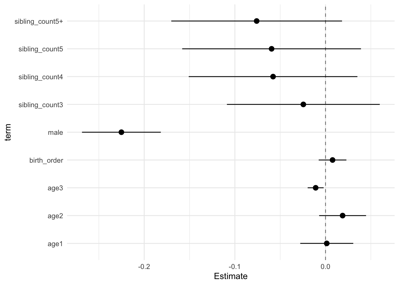
Add Birth Order Factor
Model Summary
model_genes_m3 <- with(data_used, lmer(outcome ~ birth_order_nonlinear + poly(age, degree = 3, raw = T)+ male + sibling_count +
                                         (1 | mother_pidlink), REML = FALSE))
x = mitml::testEstimates(model_genes_m3, var.comp = T)

y = as_tibble(x$estimates, rownames = "id")

y = y %>%
  mutate(CI_low = Estimate - 2.576 * Std.Error,
         CI_high = Estimate + 2.576 * Std.Error) %>%
  select(CI_low, CI_high)
CI_low = y$CI_low
CI_high = y$CI_high


x$estimates = cbind(x$estimates[,1:2], CI_low, CI_high, x$estimates[,3:7])
x
##
## Call:
##
## mitml::testEstimates(model = model_genes_m3, var.comp = T)
##
## Final parameter estimates and inferences obtained from 50 imputed data sets.
##
## Estimate Std.Error CI_low CI_high t.value df P(>|t|) RIV FMI
## (Intercept) 0.129 0.029 0.054 0.205 4.417 832.591 0.000 0.320 0.244
## birth_order_nonlinear2 0.026 0.026 -0.040 0.092 1.016 345.978 0.311 0.603 0.380
## birth_order_nonlinear3 0.027 0.032 -0.055 0.109 0.852 292.014 0.395 0.694 0.414
## birth_order_nonlinear4 0.056 0.038 -0.041 0.153 1.497 350.126 0.135 0.598 0.378
## birth_order_nonlinear5 0.092 0.050 -0.037 0.221 1.830 283.660 0.068 0.711 0.420
## birth_order_nonlinear5+ 0.023 0.045 -0.092 0.139 0.520 326.717 0.604 0.632 0.391
## poly(age, degree = 3, raw = T)1 0.001 0.011 -0.028 0.030 0.113 6159.729 0.910 0.098 0.089
## poly(age, degree = 3, raw = T)2 0.019 0.010 -0.007 0.045 1.875 3561.133 0.061 0.133 0.118
## poly(age, degree = 3, raw = T)3 -0.011 0.003 -0.020 -0.002 -3.175 10059.129 0.002 0.075 0.070
## male -0.225 0.017 -0.269 -0.182 -13.353 2376.271 0.000 0.168 0.144
## sibling_count3 -0.026 0.033 -0.113 0.060 -0.786 631.590 0.432 0.386 0.281
## sibling_count4 -0.065 0.038 -0.163 0.033 -1.715 298.639 0.087 0.681 0.409
## sibling_count5 -0.073 0.039 -0.175 0.028 -1.865 380.086 0.063 0.560 0.362
## sibling_count5+ -0.076 0.037 -0.172 0.019 -2.062 357.713 0.040 0.588 0.374
##
## Estimate
## Intercept~~Intercept|mother_pidlink 0.059
## Residual~~Residual 0.926
## ICC|mother_pidlink 0.060
##
## Unadjusted hypothesis test as appropriate in larger samples.x$estimates %>%
as.data.frame() %>%
tibble::rownames_to_column("term") %>%
filter(term != "(Intercept)") %>%
mutate(term = str_replace_all(term, "poly\\(", "")) %>%
mutate(term = str_replace_all(term, ", degree = 3, raw = T\\)", "")) %>%
ggplot(aes(x= term, y = Estimate, ymin = CI_low, ymax = CI_high)) +
geom_hline(yintercept = 0, linetype = "dashed", alpha = 0.5) +
geom_pointrange() +
coord_flip() +
theme_minimal()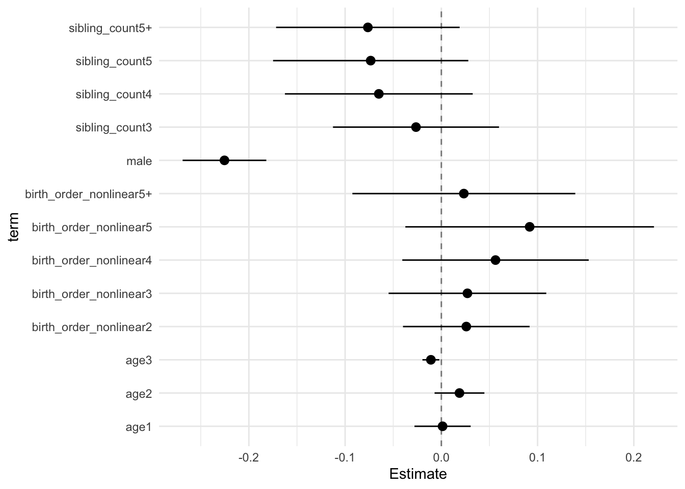
Add Interaction
Model Summary
model_genes_m4 <- with(data_used, lmer(outcome ~ count_birth_order + poly(age, degree = 3, raw = T)+ male  +
                                         (1 | mother_pidlink), REML = FALSE))
x = mitml::testEstimates(model_genes_m4, var.comp = T)

y = as_tibble(x$estimates, rownames = "id")

y = y %>%
  mutate(CI_low = Estimate - 2.576 * Std.Error,
         CI_high = Estimate + 2.576 * Std.Error) %>%
  select(CI_low, CI_high)
CI_low = y$CI_low
CI_high = y$CI_high


x$estimates = cbind(x$estimates[,1:2], CI_low, CI_high, x$estimates[,3:7])
x
##
## Call:
##
## mitml::testEstimates(model = model_genes_m4, var.comp = T)
##
## Final parameter estimates and inferences obtained from 50 imputed data sets.
##
## Estimate Std.Error CI_low CI_high t.value df P(>|t|) RIV FMI
## (Intercept) 0.132 0.032 0.049 0.215 4.092 1113.263 0.000 0.265 0.211
## count_birth_order2/2 0.018 0.051 -0.113 0.149 0.352 512.136 0.725 0.448 0.312
## count_birth_order1/3 -0.047 0.042 -0.154 0.060 -1.129 1061.007 0.259 0.274 0.216
## count_birth_order2/3 0.025 0.052 -0.108 0.157 0.478 383.167 0.633 0.557 0.361
## count_birth_order3/3 -0.003 0.051 -0.134 0.128 -0.057 769.110 0.955 0.338 0.254
## count_birth_order1/4 -0.053 0.053 -0.190 0.084 -0.988 249.071 0.324 0.797 0.448
## count_birth_order2/4 -0.051 0.051 -0.182 0.081 -0.992 626.588 0.321 0.388 0.282
## count_birth_order3/4 -0.041 0.059 -0.193 0.112 -0.686 434.265 0.493 0.506 0.339
## count_birth_order4/4 -0.026 0.057 -0.172 0.119 -0.466 506.254 0.641 0.452 0.314
## count_birth_order1/5 -0.058 0.059 -0.209 0.094 -0.982 270.344 0.327 0.741 0.430
## count_birth_order2/5 -0.048 0.063 -0.212 0.115 -0.763 374.321 0.446 0.567 0.365
## count_birth_order3/5 -0.049 0.067 -0.220 0.122 -0.737 497.723 0.462 0.457 0.317
## count_birth_order4/5 -0.006 0.076 -0.203 0.191 -0.080 326.362 0.937 0.633 0.391
## count_birth_order5/5 -0.034 0.071 -0.215 0.148 -0.476 340.916 0.635 0.611 0.383
## count_birth_order1/5+ -0.088 0.051 -0.219 0.043 -1.735 346.075 0.084 0.603 0.380
## count_birth_order2/5+ -0.073 0.053 -0.209 0.063 -1.384 514.831 0.167 0.446 0.311
## count_birth_order3/5+ -0.051 0.062 -0.211 0.110 -0.817 282.011 0.415 0.715 0.421
## count_birth_order4/5+ -0.013 0.063 -0.174 0.148 -0.213 396.772 0.832 0.542 0.355
## count_birth_order5/5+ 0.059 0.065 -0.109 0.228 0.905 496.252 0.366 0.458 0.317
## count_birth_order5+/5+ -0.055 0.045 -0.172 0.061 -1.223 718.775 0.222 0.353 0.263
## poly(age, degree = 3, raw = T)1 0.001 0.011 -0.028 0.030 0.093 6055.282 0.926 0.099 0.090
## poly(age, degree = 3, raw = T)2 0.019 0.010 -0.007 0.045 1.873 3711.691 0.061 0.130 0.115
## poly(age, degree = 3, raw = T)3 -0.011 0.003 -0.020 -0.002 -3.154 10257.070 0.002 0.074 0.069
## male -0.225 0.017 -0.269 -0.182 -13.352 2373.810 0.000 0.168 0.144
##
## Estimate
## Intercept~~Intercept|mother_pidlink 0.059
## Residual~~Residual 0.925
## ICC|mother_pidlink 0.060
##
## Unadjusted hypothesis test as appropriate in larger samples.x$estimates %>%
as.data.frame() %>%
tibble::rownames_to_column("term") %>%
filter(term != "(Intercept)") %>%
mutate(term = str_replace_all(term, "poly\\(", "")) %>%
mutate(term = str_replace_all(term, ", degree = 3, raw = T\\)", "")) %>%
ggplot(aes(x= term, y = Estimate, ymin = CI_low, ymax = CI_high)) +
geom_hline(yintercept = 0, linetype = "dashed", alpha = 0.5) +
geom_pointrange() +
coord_flip() +
theme_minimal()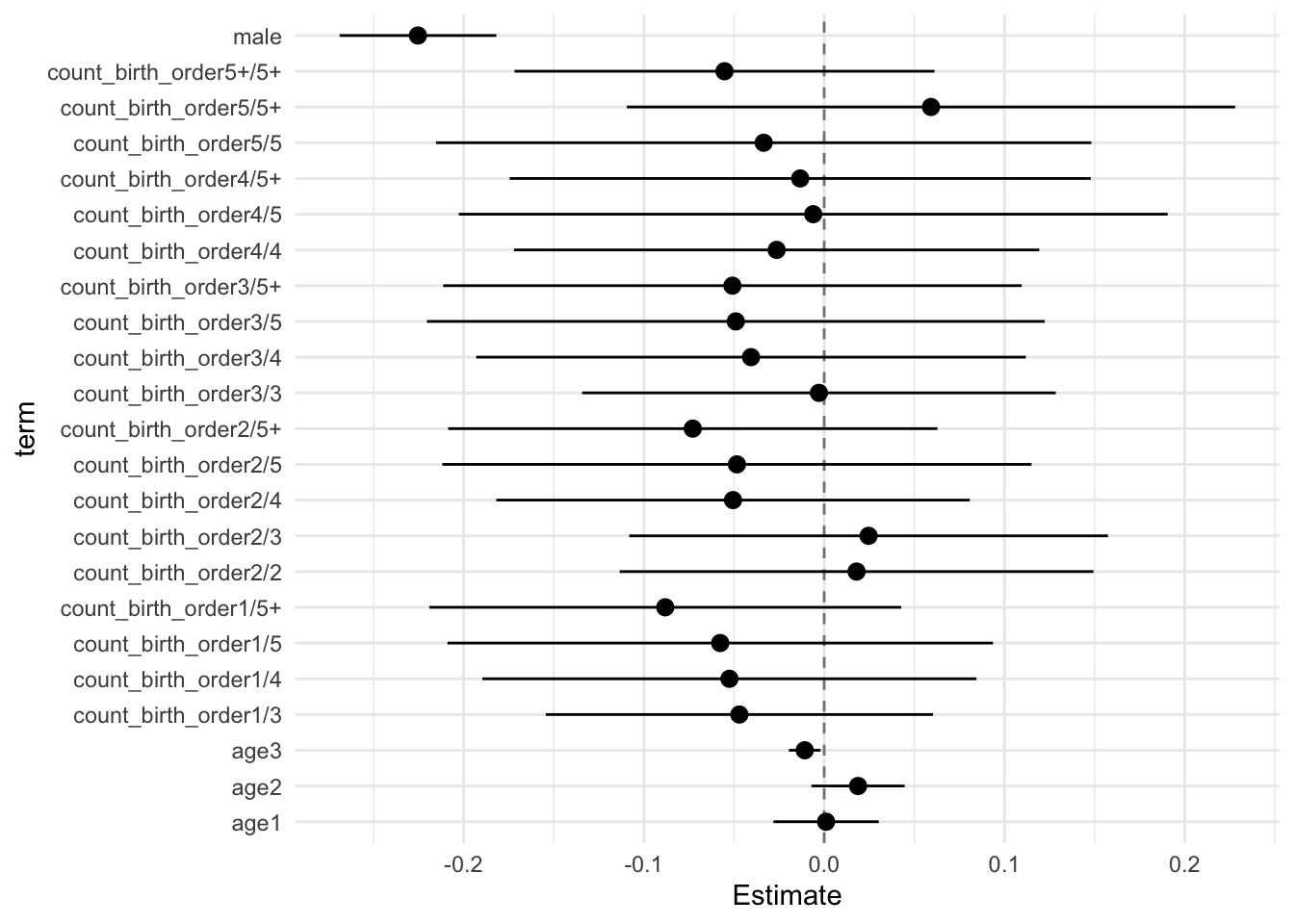
Model Comparison
anova(model_genes_m1, model_genes_m2, model_genes_m3, model_genes_m4)##
## Call:
##
## anova.mitml.result(object = model_genes_m1, model_genes_m2, model_genes_m3,
## model_genes_m4)
##
## Model comparison calculated from 50 imputed data sets.
## Combination method: D3
##
## Model 1: outcome~count_birth_order+poly(age,degree=3,raw=T)+male+(1|mother_pidlink)
## Model 2: outcome~birth_order_nonlinear+poly(age,degree=3,raw=T)+male+sibling_count+(1|mother_pidlink)
## Model 3: outcome~birth_order+poly(age,degree=3,raw=T)+male+sibling_count+(1|mother_pidlink)
## Model 4: outcome~poly(age,degree=3,raw=T)+male+sibling_count+(1|mother_pidlink)
##
## F.value df1 df2 P(>F) RIV
## 1 vs 2: 0.269 10 2904.943 0.988 0.690
## 2 vs 3: 0.839 4 1453.298 0.500 0.566
## 3 vs 4: 1.716 1 312.727 0.191 0.592Neuroticism
# Specify your outcome
data_used = data_used %>% mutate(outcome = big5_neu)
compare_birthorder_imputed(data_used = data_used)
Parental full sibling order
Basic Model
# with.mitml.list <- function (data, expr, ...)
# {
#     expr <- substitute(expr)
#     parent <- parent.frame()
#     out <- parallel::mclapply(data, function(x) eval(expr, x, parent))
#     class(out) <- c("mitml.result", "list")
#     out
# }
Model Summary
data_used = data_used %>%
  mutate(sibling_count = sibling_count_genes_factor,
         birth_order_nonlinear = birthorder_genes_factor,
         birth_order = birthorder_genes,
         count_birth_order = count_birthorder_genes)

data_used_plots = data_used[[1]]

model_genes_m1 <- with(data_used, lmer(outcome ~ poly(age, degree = 3, raw = T)+ male + sibling_count + (1 | mother_pidlink), REML = FALSE))
x = mitml::testEstimates(model_genes_m1, var.comp = T)

y = as_tibble(x$estimates, rownames = "id")

y = y %>%
  mutate(CI_low = Estimate - 2.576 * Std.Error,
         CI_high = Estimate + 2.576 * Std.Error) %>%
  select(CI_low, CI_high)
CI_low = y$CI_low
CI_high = y$CI_high


x$estimates = cbind(x$estimates[,1:2], CI_low, CI_high, x$estimates[,3:7])
x
##
## Call:
##
## mitml::testEstimates(model = model_genes_m1, var.comp = T)
##
## Final parameter estimates and inferences obtained from 50 imputed data sets.
##
## Estimate Std.Error CI_low CI_high t.value df P(>|t|) RIV FMI
## (Intercept) 0.100 0.029 0.025 0.176 3.435 551.057 0.001 0.425 0.301
## poly(age, degree = 3, raw = T)1 -0.124 0.011 -0.153 -0.095 -10.975 5479.484 0.000 0.104 0.095
## poly(age, degree = 3, raw = T)2 0.009 0.010 -0.018 0.035 0.856 1787.616 0.392 0.198 0.166
## poly(age, degree = 3, raw = T)3 0.000 0.003 -0.009 0.009 0.039 5283.733 0.969 0.107 0.097
## male -0.261 0.017 -0.304 -0.219 -15.803 2987.802 0.000 0.147 0.129
## sibling_count3 0.009 0.034 -0.079 0.097 0.263 464.860 0.792 0.481 0.328
## sibling_count4 0.002 0.034 -0.086 0.090 0.062 481.084 0.950 0.469 0.322
## sibling_count5 0.020 0.038 -0.079 0.119 0.520 339.413 0.603 0.613 0.384
## sibling_count5+ 0.048 0.033 -0.036 0.133 1.474 421.022 0.141 0.518 0.344
##
## Estimate
## Intercept~~Intercept|mother_pidlink 0.082
## Residual~~Residual 0.887
## ICC|mother_pidlink 0.085
##
## Unadjusted hypothesis test as appropriate in larger samples.x$estimates %>%
as.data.frame() %>%
tibble::rownames_to_column("term") %>%
filter(term != "(Intercept)") %>%
mutate(term = str_replace_all(term, "poly\\(", "")) %>%
mutate(term = str_replace_all(term, ", degree = 3, raw = T\\)", "")) %>%
ggplot(aes(x= term, y = Estimate, ymin = CI_low, ymax = CI_high)) +
geom_hline(yintercept = 0, linetype = "dashed", alpha = 0.5) +
geom_pointrange() +
coord_flip() +
theme_minimal()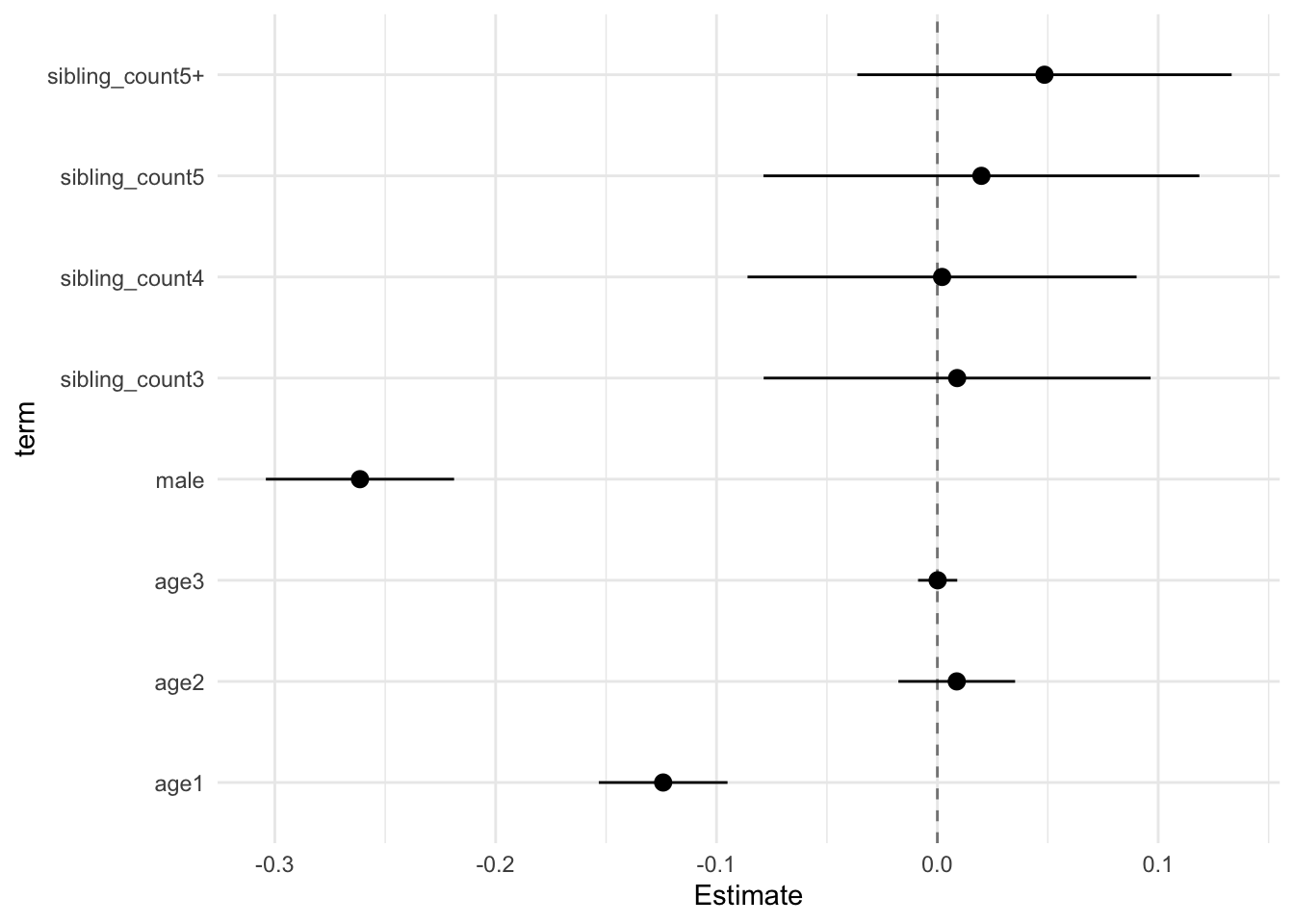
Add Birth Order Linear
Model Summary
model_genes_m2 <- with(data_used, lmer(outcome ~ birth_order + poly(age, degree = 3, raw = T)+ male + sibling_count +
                                         (1 | mother_pidlink), REML = FALSE))
x = mitml::testEstimates(model_genes_m2, var.comp = T)

y = as_tibble(x$estimates, rownames = "id")

y = y %>%
  mutate(CI_low = Estimate - 2.576 * Std.Error,
         CI_high = Estimate + 2.576 * Std.Error) %>%
  select(CI_low, CI_high)
CI_low = y$CI_low
CI_high = y$CI_high


x$estimates = cbind(x$estimates[,1:2], CI_low, CI_high, x$estimates[,3:7])
x
##
## Call:
##
## mitml::testEstimates(model = model_genes_m2, var.comp = T)
##
## Final parameter estimates and inferences obtained from 50 imputed data sets.
##
## Estimate Std.Error CI_low CI_high t.value df P(>|t|) RIV FMI
## (Intercept) 0.100 0.029 0.024 0.176 3.394 699.724 0.001 0.360 0.267
## birth_order 0.000 0.006 -0.015 0.015 0.049 411.710 0.961 0.527 0.348
## poly(age, degree = 3, raw = T)1 -0.124 0.011 -0.153 -0.095 -10.904 5128.009 0.000 0.108 0.098
## poly(age, degree = 3, raw = T)2 0.009 0.010 -0.018 0.035 0.858 1855.793 0.391 0.194 0.163
## poly(age, degree = 3, raw = T)3 0.000 0.003 -0.009 0.009 0.038 5707.913 0.970 0.102 0.093
## male -0.261 0.017 -0.304 -0.219 -15.798 2961.675 0.000 0.148 0.129
## sibling_count3 0.009 0.034 -0.079 0.097 0.258 450.632 0.797 0.492 0.333
## sibling_count4 0.002 0.035 -0.088 0.092 0.053 440.546 0.958 0.500 0.337
## sibling_count5 0.020 0.040 -0.084 0.123 0.486 286.752 0.627 0.705 0.417
## sibling_count5+ 0.048 0.037 -0.048 0.144 1.282 329.334 0.201 0.628 0.389
##
## Estimate
## Intercept~~Intercept|mother_pidlink 0.082
## Residual~~Residual 0.887
## ICC|mother_pidlink 0.085
##
## Unadjusted hypothesis test as appropriate in larger samples.x$estimates %>%
as.data.frame() %>%
tibble::rownames_to_column("term") %>%
filter(term != "(Intercept)") %>%
mutate(term = str_replace_all(term, "poly\\(", "")) %>%
mutate(term = str_replace_all(term, ", degree = 3, raw = T\\)", "")) %>%
ggplot(aes(x= term, y = Estimate, ymin = CI_low, ymax = CI_high)) +
geom_hline(yintercept = 0, linetype = "dashed", alpha = 0.5) +
geom_pointrange() +
coord_flip() +
theme_minimal()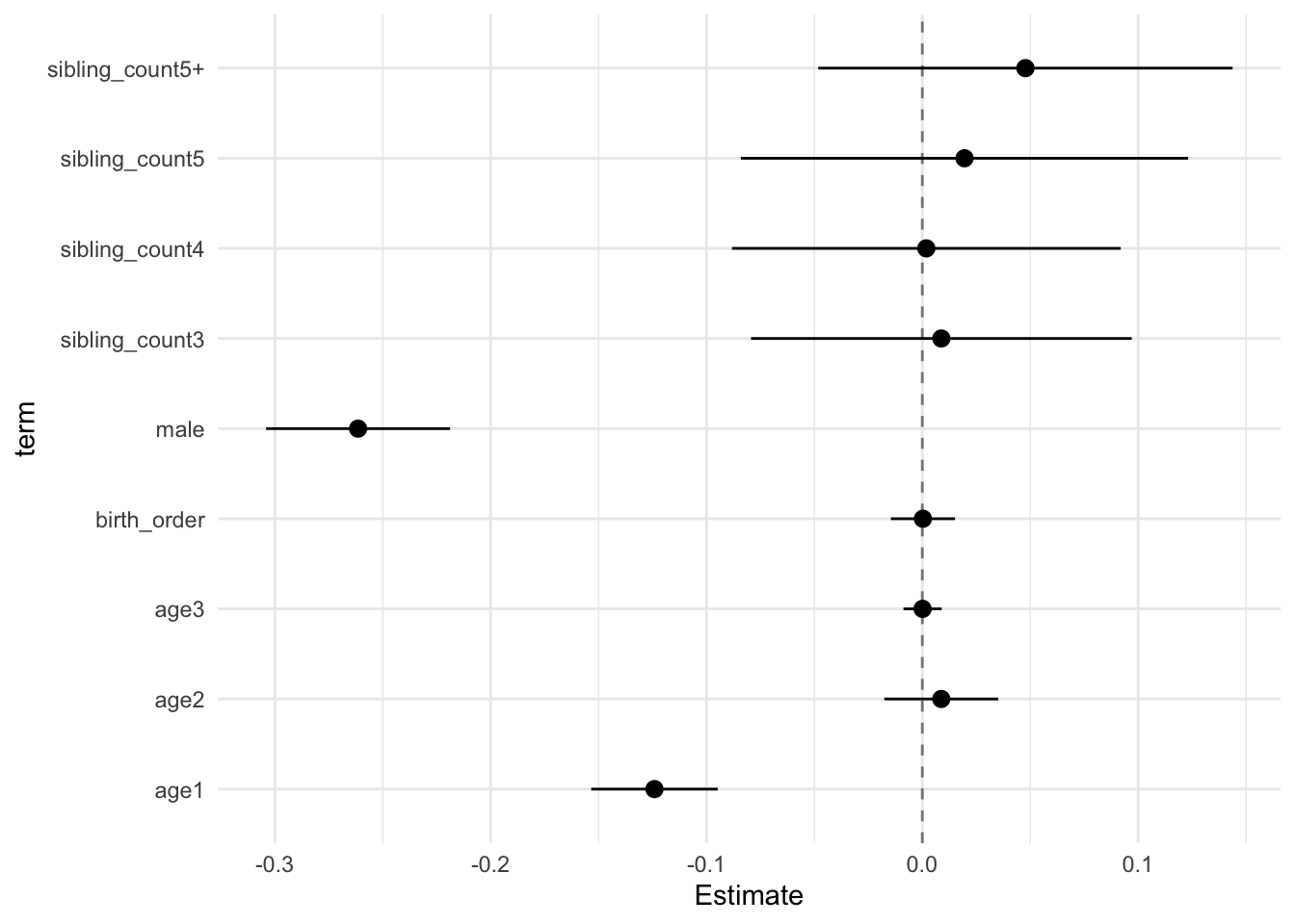
Add Birth Order Factor
Model Summary
model_genes_m3 <- with(data_used, lmer(outcome ~ birth_order_nonlinear + poly(age, degree = 3, raw = T)+ male + sibling_count +
                                         (1 | mother_pidlink), REML = FALSE))
x = mitml::testEstimates(model_genes_m3, var.comp = T)

y = as_tibble(x$estimates, rownames = "id")

y = y %>%
  mutate(CI_low = Estimate - 2.576 * Std.Error,
         CI_high = Estimate + 2.576 * Std.Error) %>%
  select(CI_low, CI_high)
CI_low = y$CI_low
CI_high = y$CI_high


x$estimates = cbind(x$estimates[,1:2], CI_low, CI_high, x$estimates[,3:7])
x
##
## Call:
##
## mitml::testEstimates(model = model_genes_m3, var.comp = T)
##
## Final parameter estimates and inferences obtained from 50 imputed data sets.
##
## Estimate Std.Error CI_low CI_high t.value df P(>|t|) RIV FMI
## (Intercept) 0.103 0.031 0.024 0.182 3.378 524.852 0.001 0.440 0.308
## birth_order_nonlinear2 -0.009 0.026 -0.075 0.058 -0.331 308.405 0.741 0.663 0.402
## birth_order_nonlinear3 0.019 0.032 -0.063 0.101 0.589 271.464 0.556 0.739 0.429
## birth_order_nonlinear4 -0.040 0.036 -0.133 0.054 -1.087 403.341 0.278 0.535 0.352
## birth_order_nonlinear5 -0.033 0.047 -0.155 0.088 -0.708 387.466 0.480 0.552 0.359
## birth_order_nonlinear5+ 0.016 0.045 -0.099 0.132 0.367 318.922 0.714 0.645 0.396
## poly(age, degree = 3, raw = T)1 -0.124 0.011 -0.154 -0.095 -10.925 4954.707 0.000 0.110 0.100
## poly(age, degree = 3, raw = T)2 0.009 0.010 -0.018 0.035 0.855 1858.249 0.392 0.194 0.163
## poly(age, degree = 3, raw = T)3 0.000 0.003 -0.009 0.009 0.047 5610.668 0.963 0.103 0.094
## male -0.261 0.017 -0.304 -0.219 -15.777 2921.707 0.000 0.149 0.130
## sibling_count3 0.004 0.035 -0.086 0.094 0.115 450.112 0.909 0.492 0.333
## sibling_count4 0.006 0.035 -0.085 0.097 0.169 494.936 0.866 0.459 0.317
## sibling_count5 0.027 0.041 -0.079 0.132 0.652 304.149 0.515 0.671 0.405
## sibling_count5+ 0.048 0.038 -0.049 0.145 1.265 321.988 0.207 0.640 0.394
##
## Estimate
## Intercept~~Intercept|mother_pidlink 0.082
## Residual~~Residual 0.887
## ICC|mother_pidlink 0.085
##
## Unadjusted hypothesis test as appropriate in larger samples.x$estimates %>%
as.data.frame() %>%
tibble::rownames_to_column("term") %>%
filter(term != "(Intercept)") %>%
mutate(term = str_replace_all(term, "poly\\(", "")) %>%
mutate(term = str_replace_all(term, ", degree = 3, raw = T\\)", "")) %>%
ggplot(aes(x= term, y = Estimate, ymin = CI_low, ymax = CI_high)) +
geom_hline(yintercept = 0, linetype = "dashed", alpha = 0.5) +
geom_pointrange() +
coord_flip() +
theme_minimal()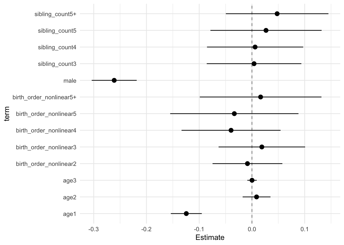
Add Interaction
Model Summary
model_genes_m4 <- with(data_used, lmer(outcome ~ count_birth_order + poly(age, degree = 3, raw = T)+ male  +
                                         (1 | mother_pidlink), REML = FALSE))
x = mitml::testEstimates(model_genes_m4, var.comp = T)

y = as_tibble(x$estimates, rownames = "id")

y = y %>%
  mutate(CI_low = Estimate - 2.576 * Std.Error,
         CI_high = Estimate + 2.576 * Std.Error) %>%
  select(CI_low, CI_high)
CI_low = y$CI_low
CI_high = y$CI_high


x$estimates = cbind(x$estimates[,1:2], CI_low, CI_high, x$estimates[,3:7])
x
##
## Call:
##
## mitml::testEstimates(model = model_genes_m4, var.comp = T)
##
## Final parameter estimates and inferences obtained from 50 imputed data sets.
##
## Estimate Std.Error CI_low CI_high t.value df P(>|t|) RIV FMI
## (Intercept) 0.105 0.034 0.016 0.194 3.039 495.390 0.002 0.459 0.317
## count_birth_order2/2 -0.013 0.050 -0.143 0.116 -0.265 510.677 0.791 0.449 0.312
## count_birth_order1/3 -0.013 0.045 -0.129 0.102 -0.296 448.678 0.767 0.494 0.333
## count_birth_order2/3 0.006 0.050 -0.123 0.134 0.112 476.301 0.911 0.472 0.324
## count_birth_order3/3 0.036 0.055 -0.105 0.177 0.662 382.480 0.508 0.557 0.361
## count_birth_order1/4 0.008 0.049 -0.118 0.134 0.162 399.475 0.871 0.539 0.353
## count_birth_order2/4 0.009 0.054 -0.130 0.147 0.165 377.233 0.869 0.563 0.364
## count_birth_order3/4 0.010 0.063 -0.153 0.173 0.157 269.782 0.875 0.743 0.430
## count_birth_order4/4 -0.046 0.056 -0.190 0.098 -0.829 530.060 0.408 0.437 0.307
## count_birth_order1/5 0.055 0.060 -0.098 0.208 0.923 246.801 0.357 0.804 0.450
## count_birth_order2/5 -0.023 0.067 -0.196 0.151 -0.341 252.677 0.733 0.787 0.445
## count_birth_order3/5 0.056 0.070 -0.125 0.237 0.795 314.127 0.427 0.653 0.399
## count_birth_order4/5 -0.011 0.075 -0.203 0.182 -0.143 358.461 0.887 0.587 0.373
## count_birth_order5/5 -0.031 0.069 -0.209 0.148 -0.442 369.069 0.659 0.573 0.368
## count_birth_order1/5+ 0.039 0.052 -0.096 0.175 0.751 278.844 0.453 0.722 0.423
## count_birth_order2/5+ 0.039 0.054 -0.100 0.179 0.727 392.733 0.468 0.546 0.356
## count_birth_order3/5+ 0.051 0.063 -0.112 0.214 0.812 251.325 0.418 0.791 0.446
## count_birth_order4/5+ 0.017 0.066 -0.154 0.188 0.260 262.987 0.795 0.759 0.436
## count_birth_order5/5+ 0.033 0.064 -0.132 0.198 0.516 576.271 0.606 0.412 0.294
## count_birth_order5+/5+ 0.063 0.046 -0.056 0.182 1.364 571.235 0.173 0.414 0.295
## poly(age, degree = 3, raw = T)1 -0.125 0.011 -0.154 -0.095 -10.945 5046.216 0.000 0.109 0.099
## poly(age, degree = 3, raw = T)2 0.009 0.010 -0.018 0.035 0.845 1849.186 0.398 0.194 0.164
## poly(age, degree = 3, raw = T)3 0.000 0.003 -0.009 0.009 0.062 5610.551 0.951 0.103 0.094
## male -0.261 0.017 -0.304 -0.219 -15.762 2827.548 0.000 0.152 0.132
##
## Estimate
## Intercept~~Intercept|mother_pidlink 0.082
## Residual~~Residual 0.886
## ICC|mother_pidlink 0.085
##
## Unadjusted hypothesis test as appropriate in larger samples.x$estimates %>%
as.data.frame() %>%
tibble::rownames_to_column("term") %>%
filter(term != "(Intercept)") %>%
mutate(term = str_replace_all(term, "poly\\(", "")) %>%
mutate(term = str_replace_all(term, ", degree = 3, raw = T\\)", "")) %>%
ggplot(aes(x= term, y = Estimate, ymin = CI_low, ymax = CI_high)) +
geom_hline(yintercept = 0, linetype = "dashed", alpha = 0.5) +
geom_pointrange() +
coord_flip() +
theme_minimal()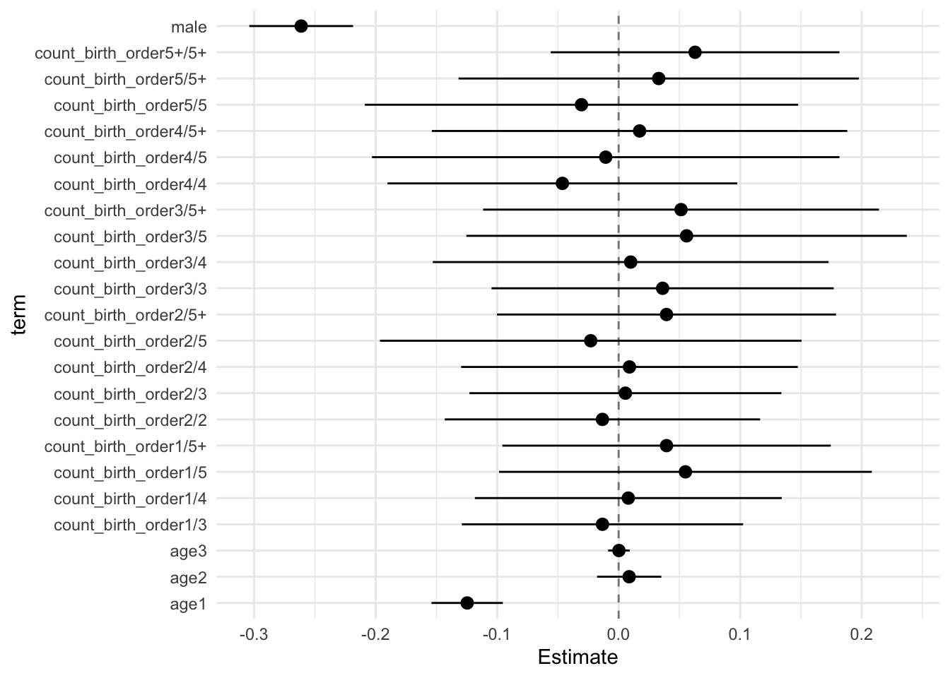
Model Comparison
anova(model_genes_m1, model_genes_m2, model_genes_m3, model_genes_m4)##
## Call:
##
## anova.mitml.result(object = model_genes_m1, model_genes_m2, model_genes_m3,
## model_genes_m4)
##
## Model comparison calculated from 50 imputed data sets.
## Combination method: D3
##
## Model 1: outcome~count_birth_order+poly(age,degree=3,raw=T)+male+(1|mother_pidlink)
## Model 2: outcome~birth_order_nonlinear+poly(age,degree=3,raw=T)+male+sibling_count+(1|mother_pidlink)
## Model 3: outcome~birth_order+poly(age,degree=3,raw=T)+male+sibling_count+(1|mother_pidlink)
## Model 4: outcome~poly(age,degree=3,raw=T)+male+sibling_count+(1|mother_pidlink)
##
## F.value df1 df2 P(>F) RIV
## 1 vs 2: 0.206 10 3135.163 0.996 0.647
## 2 vs 3: 0.683 4 1125.025 0.604 0.699
## 3 vs 4: 0.002 1 362.589 0.962 0.526Conscientiousness
# Specify your outcome
data_used = data_used %>% mutate(outcome = big5_con)
data_used_plots <- data_used[[1]]

compare_birthorder_imputed(data_used = data_used)
Parental full sibling order
Basic Model
# with.mitml.list <- function (data, expr, ...)
# {
#     expr <- substitute(expr)
#     parent <- parent.frame()
#     out <- parallel::mclapply(data, function(x) eval(expr, x, parent))
#     class(out) <- c("mitml.result", "list")
#     out
# }
Model Summary
data_used = data_used %>%
  mutate(sibling_count = sibling_count_genes_factor,
         birth_order_nonlinear = birthorder_genes_factor,
         birth_order = birthorder_genes,
         count_birth_order = count_birthorder_genes)

data_used_plots = data_used[[1]]

model_genes_m1 <- with(data_used, lmer(outcome ~ poly(age, degree = 3, raw = T)+ male + sibling_count + (1 | mother_pidlink), REML = FALSE))
x = mitml::testEstimates(model_genes_m1, var.comp = T)

y = as_tibble(x$estimates, rownames = "id")

y = y %>%
  mutate(CI_low = Estimate - 2.576 * Std.Error,
         CI_high = Estimate + 2.576 * Std.Error) %>%
  select(CI_low, CI_high)
CI_low = y$CI_low
CI_high = y$CI_high


x$estimates = cbind(x$estimates[,1:2], CI_low, CI_high, x$estimates[,3:7])
x
##
## Call:
##
## mitml::testEstimates(model = model_genes_m1, var.comp = T)
##
## Final parameter estimates and inferences obtained from 50 imputed data sets.
##
## Estimate Std.Error CI_low CI_high t.value df P(>|t|) RIV FMI
## (Intercept) 0.035 0.027 -0.034 0.104 1.318 1288.292 0.188 0.242 0.196
## poly(age, degree = 3, raw = T)1 0.219 0.011 0.191 0.248 19.680 5144.962 0.000 0.108 0.098
## poly(age, degree = 3, raw = T)2 -0.068 0.010 -0.093 -0.042 -6.797 2915.562 0.000 0.149 0.130
## poly(age, degree = 3, raw = T)3 0.004 0.003 -0.004 0.013 1.304 5533.901 0.192 0.104 0.094
## male 0.049 0.017 0.005 0.092 2.882 1609.155 0.004 0.211 0.176
## sibling_count3 -0.016 0.034 -0.105 0.072 -0.476 367.731 0.635 0.575 0.368
## sibling_count4 -0.012 0.032 -0.095 0.070 -0.385 702.640 0.700 0.359 0.266
## sibling_count5 0.002 0.035 -0.088 0.092 0.057 581.511 0.955 0.409 0.293
## sibling_count5+ 0.035 0.030 -0.041 0.111 1.180 987.080 0.238 0.287 0.224
##
## Estimate
## Intercept~~Intercept|mother_pidlink 0.051
## Residual~~Residual 0.905
## ICC|mother_pidlink 0.053
##
## Unadjusted hypothesis test as appropriate in larger samples.x$estimates %>%
as.data.frame() %>%
tibble::rownames_to_column("term") %>%
filter(term != "(Intercept)") %>%
mutate(term = str_replace_all(term, "poly\\(", "")) %>%
mutate(term = str_replace_all(term, ", degree = 3, raw = T\\)", "")) %>%
ggplot(aes(x= term, y = Estimate, ymin = CI_low, ymax = CI_high)) +
geom_hline(yintercept = 0, linetype = "dashed", alpha = 0.5) +
geom_pointrange() +
coord_flip() +
theme_minimal()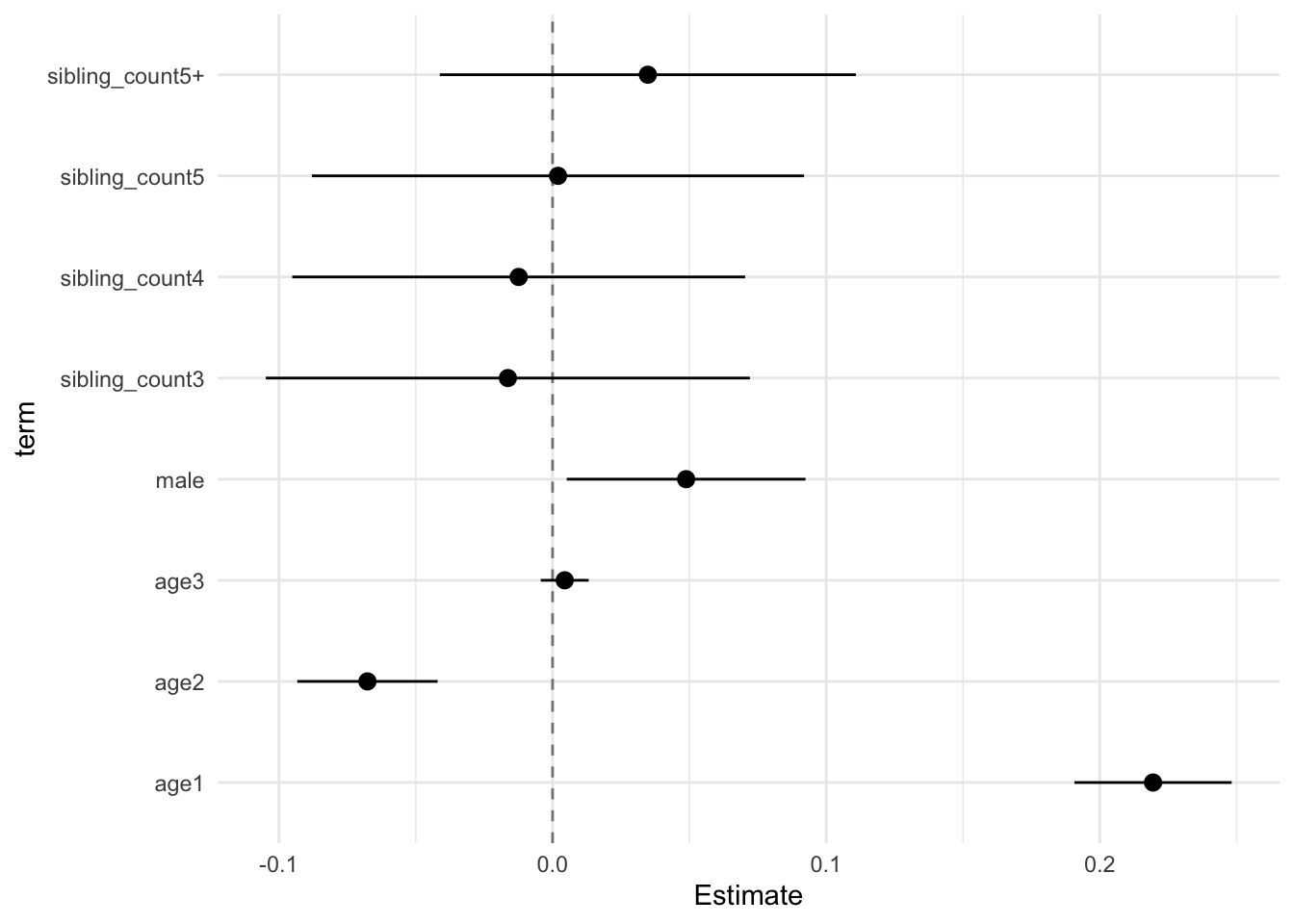
Add Birth Order Linear
Model Summary
model_genes_m2 <- with(data_used, lmer(outcome ~ birth_order + poly(age, degree = 3, raw = T)+ male + sibling_count +
                                         (1 | mother_pidlink), REML = FALSE))
x = mitml::testEstimates(model_genes_m2, var.comp = T)

y = as_tibble(x$estimates, rownames = "id")

y = y %>%
  mutate(CI_low = Estimate - 2.576 * Std.Error,
         CI_high = Estimate + 2.576 * Std.Error) %>%
  select(CI_low, CI_high)
CI_low = y$CI_low
CI_high = y$CI_high


x$estimates = cbind(x$estimates[,1:2], CI_low, CI_high, x$estimates[,3:7])
x
##
## Call:
##
## mitml::testEstimates(model = model_genes_m2, var.comp = T)
##
## Final parameter estimates and inferences obtained from 50 imputed data sets.
##
## Estimate Std.Error CI_low CI_high t.value df P(>|t|) RIV FMI
## (Intercept) 0.038 0.028 -0.034 0.111 1.363 1055.475 0.173 0.275 0.217
## birth_order -0.002 0.006 -0.018 0.014 -0.349 248.201 0.727 0.800 0.449
## poly(age, degree = 3, raw = T)1 0.219 0.011 0.190 0.248 19.438 4072.200 0.000 0.123 0.110
## poly(age, degree = 3, raw = T)2 -0.068 0.010 -0.093 -0.042 -6.790 2732.288 0.000 0.155 0.135
## poly(age, degree = 3, raw = T)3 0.004 0.003 -0.004 0.013 1.313 4981.474 0.189 0.110 0.100
## male 0.049 0.017 0.005 0.092 2.882 1616.078 0.004 0.211 0.175
## sibling_count3 -0.015 0.034 -0.104 0.073 -0.447 374.940 0.655 0.566 0.365
## sibling_count4 -0.010 0.033 -0.094 0.074 -0.318 675.038 0.751 0.369 0.272
## sibling_count5 0.005 0.036 -0.089 0.098 0.134 498.681 0.893 0.457 0.316
## sibling_count5+ 0.040 0.034 -0.048 0.128 1.181 540.286 0.238 0.431 0.304
##
## Estimate
## Intercept~~Intercept|mother_pidlink 0.051
## Residual~~Residual 0.905
## ICC|mother_pidlink 0.053
##
## Unadjusted hypothesis test as appropriate in larger samples.x$estimates %>%
as.data.frame() %>%
tibble::rownames_to_column("term") %>%
filter(term != "(Intercept)") %>%
mutate(term = str_replace_all(term, "poly\\(", "")) %>%
mutate(term = str_replace_all(term, ", degree = 3, raw = T\\)", "")) %>%
ggplot(aes(x= term, y = Estimate, ymin = CI_low, ymax = CI_high)) +
geom_hline(yintercept = 0, linetype = "dashed", alpha = 0.5) +
geom_pointrange() +
coord_flip() +
theme_minimal()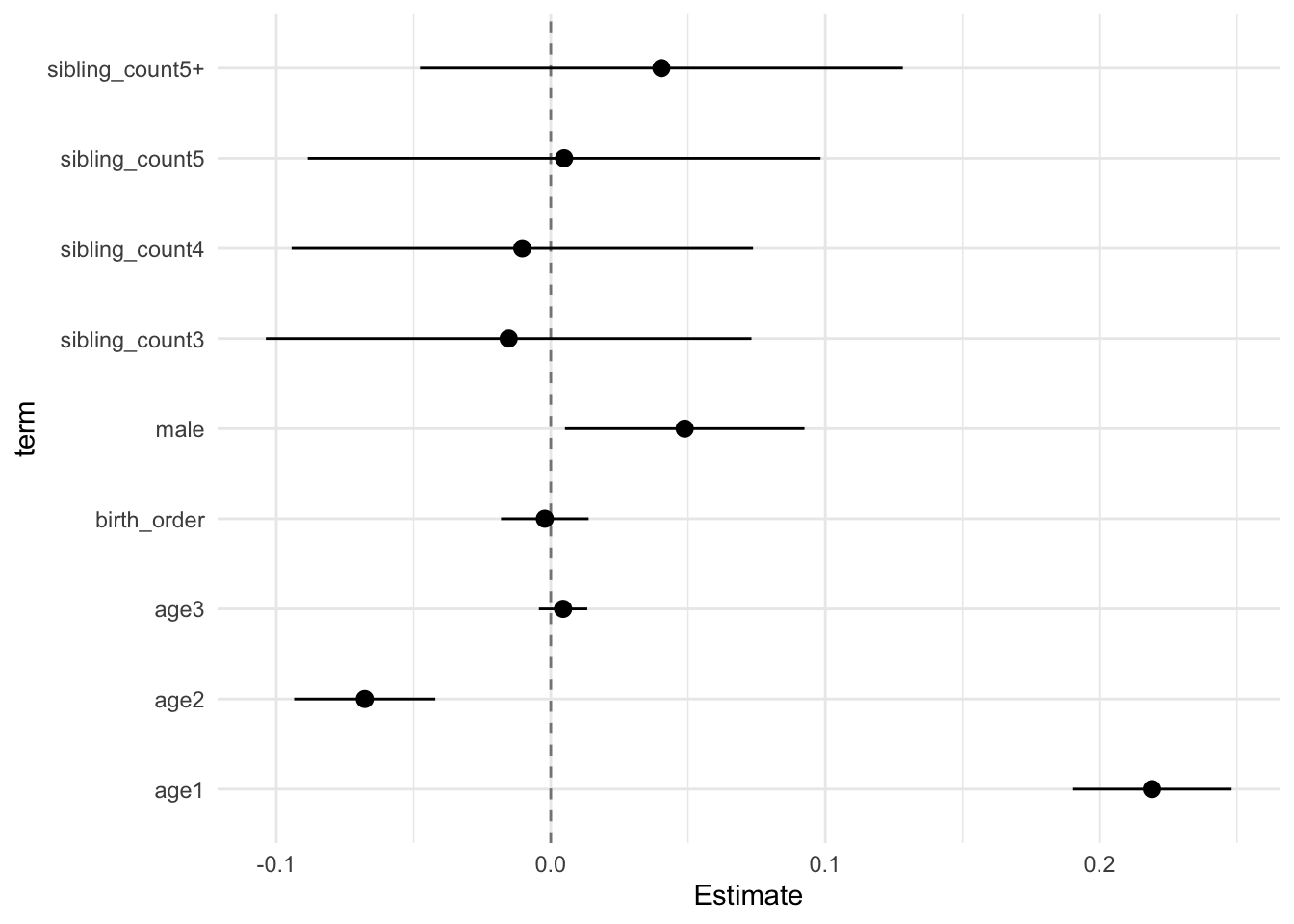
Add Birth Order Factor
Model Summary
model_genes_m3 <- with(data_used, lmer(outcome ~ birth_order_nonlinear + poly(age, degree = 3, raw = T)+ male + sibling_count +
                                         (1 | mother_pidlink), REML = FALSE))
x = mitml::testEstimates(model_genes_m3, var.comp = T)

y = as_tibble(x$estimates, rownames = "id")

y = y %>%
  mutate(CI_low = Estimate - 2.576 * Std.Error,
         CI_high = Estimate + 2.576 * Std.Error) %>%
  select(CI_low, CI_high)
CI_low = y$CI_low
CI_high = y$CI_high


x$estimates = cbind(x$estimates[,1:2], CI_low, CI_high, x$estimates[,3:7])
x
##
## Call:
##
## mitml::testEstimates(model = model_genes_m3, var.comp = T)
##
## Final parameter estimates and inferences obtained from 50 imputed data sets.
##
## Estimate Std.Error CI_low CI_high t.value df P(>|t|) RIV FMI
## (Intercept) 0.042 0.028 -0.031 0.115 1.482 1030.906 0.139 0.279 0.220
## birth_order_nonlinear2 -0.019 0.025 -0.083 0.045 -0.762 380.523 0.447 0.560 0.362
## birth_order_nonlinear3 -0.003 0.033 -0.088 0.082 -0.091 228.423 0.927 0.863 0.468
## birth_order_nonlinear4 -0.015 0.042 -0.124 0.093 -0.366 186.286 0.715 1.053 0.518
## birth_order_nonlinear5 -0.016 0.048 -0.141 0.108 -0.337 320.248 0.737 0.642 0.395
## birth_order_nonlinear5+ -0.006 0.048 -0.129 0.116 -0.129 222.729 0.897 0.883 0.474
## poly(age, degree = 3, raw = T)1 0.219 0.011 0.190 0.248 19.453 4051.065 0.000 0.124 0.110
## poly(age, degree = 3, raw = T)2 -0.068 0.010 -0.093 -0.042 -6.781 2683.513 0.000 0.156 0.136
## poly(age, degree = 3, raw = T)3 0.004 0.003 -0.004 0.013 1.308 4949.134 0.191 0.110 0.100
## male 0.049 0.017 0.005 0.092 2.886 1619.273 0.004 0.211 0.175
## sibling_count3 -0.017 0.035 -0.107 0.074 -0.471 357.465 0.638 0.588 0.374
## sibling_count4 -0.010 0.034 -0.098 0.077 -0.305 571.990 0.760 0.414 0.295
## sibling_count5 0.005 0.037 -0.091 0.101 0.126 508.556 0.899 0.450 0.313
## sibling_count5+ 0.037 0.035 -0.053 0.126 1.053 496.661 0.293 0.458 0.317
##
## Estimate
## Intercept~~Intercept|mother_pidlink 0.051
## Residual~~Residual 0.904
## ICC|mother_pidlink 0.053
##
## Unadjusted hypothesis test as appropriate in larger samples.x$estimates %>%
as.data.frame() %>%
tibble::rownames_to_column("term") %>%
filter(term != "(Intercept)") %>%
mutate(term = str_replace_all(term, "poly\\(", "")) %>%
mutate(term = str_replace_all(term, ", degree = 3, raw = T\\)", "")) %>%
ggplot(aes(x= term, y = Estimate, ymin = CI_low, ymax = CI_high)) +
geom_hline(yintercept = 0, linetype = "dashed", alpha = 0.5) +
geom_pointrange() +
coord_flip() +
theme_minimal()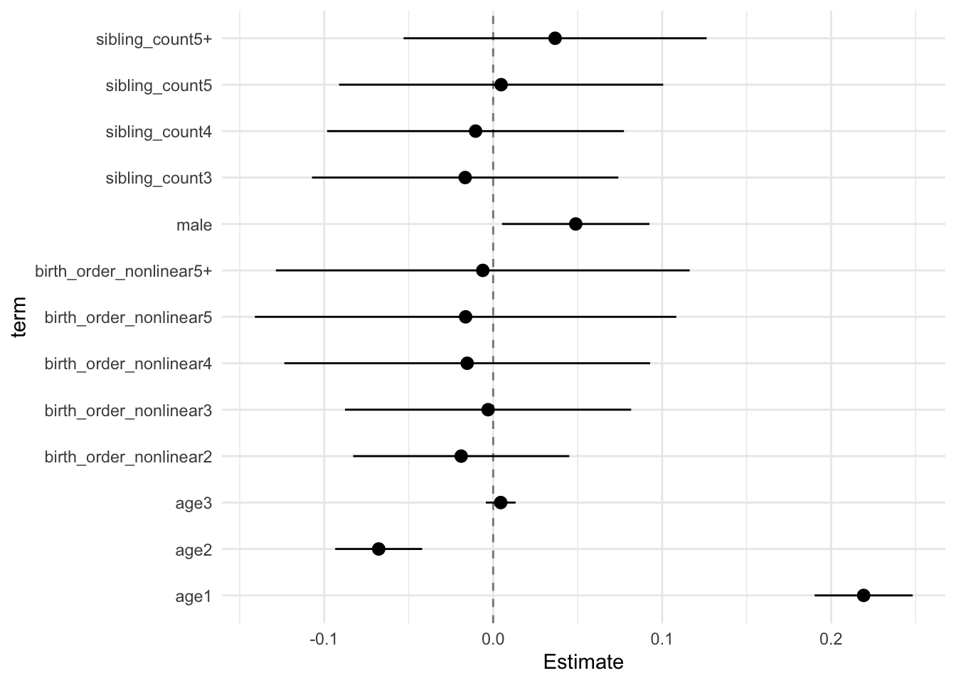
Add Interaction
Model Summary
model_genes_m4 <- with(data_used, lmer(outcome ~ count_birth_order + poly(age, degree = 3, raw = T)+ male  +
                                         (1 | mother_pidlink), REML = FALSE))
x = mitml::testEstimates(model_genes_m4, var.comp = T)

y = as_tibble(x$estimates, rownames = "id")

y = y %>%
  mutate(CI_low = Estimate - 2.576 * Std.Error,
         CI_high = Estimate + 2.576 * Std.Error) %>%
  select(CI_low, CI_high)
CI_low = y$CI_low
CI_high = y$CI_high


x$estimates = cbind(x$estimates[,1:2], CI_low, CI_high, x$estimates[,3:7])
x
##
## Call:
##
## mitml::testEstimates(model = model_genes_m4, var.comp = T)
##
## Final parameter estimates and inferences obtained from 50 imputed data sets.
##
## Estimate Std.Error CI_low CI_high t.value df P(>|t|) RIV FMI
## (Intercept) 0.052 0.033 -0.033 0.137 1.568 664.918 0.117 0.373 0.274
## count_birth_order2/2 -0.048 0.054 -0.187 0.092 -0.884 300.073 0.377 0.678 0.408
## count_birth_order1/3 -0.009 0.047 -0.129 0.112 -0.183 308.092 0.855 0.663 0.403
## count_birth_order2/3 -0.060 0.052 -0.193 0.073 -1.169 340.678 0.243 0.611 0.383
## count_birth_order3/3 -0.046 0.052 -0.181 0.089 -0.870 493.185 0.385 0.460 0.318
## count_birth_order1/4 -0.029 0.051 -0.161 0.103 -0.566 278.921 0.572 0.722 0.423
## count_birth_order2/4 -0.018 0.053 -0.154 0.119 -0.335 384.688 0.738 0.555 0.360
## count_birth_order3/4 -0.005 0.060 -0.160 0.150 -0.081 341.199 0.936 0.610 0.383
## count_birth_order4/4 -0.067 0.058 -0.216 0.083 -1.147 367.570 0.252 0.575 0.369
## count_birth_order1/5 -0.033 0.056 -0.178 0.112 -0.588 315.315 0.557 0.651 0.398
## count_birth_order2/5 -0.001 0.065 -0.168 0.166 -0.022 293.863 0.982 0.690 0.412
## count_birth_order3/5 0.027 0.069 -0.150 0.204 0.392 342.112 0.695 0.609 0.382
## count_birth_order4/5 -0.021 0.076 -0.215 0.174 -0.272 315.477 0.786 0.650 0.398
## count_birth_order5/5 -0.036 0.069 -0.214 0.143 -0.514 347.582 0.608 0.601 0.379
## count_birth_order1/5+ 0.017 0.050 -0.113 0.146 0.329 331.805 0.742 0.624 0.388
## count_birth_order2/5+ 0.006 0.056 -0.137 0.150 0.109 303.987 0.914 0.671 0.405
## count_birth_order3/5+ 0.001 0.060 -0.154 0.157 0.023 308.666 0.982 0.662 0.402
## count_birth_order4/5+ 0.048 0.068 -0.126 0.222 0.716 230.715 0.475 0.855 0.465
## count_birth_order5/5+ 0.024 0.065 -0.143 0.191 0.367 477.128 0.714 0.472 0.323
## count_birth_order5+/5+ 0.021 0.047 -0.100 0.141 0.441 442.049 0.659 0.499 0.336
## poly(age, degree = 3, raw = T)1 0.220 0.011 0.191 0.249 19.496 4169.888 0.000 0.122 0.109
## poly(age, degree = 3, raw = T)2 -0.067 0.010 -0.093 -0.042 -6.754 2723.309 0.000 0.155 0.135
## poly(age, degree = 3, raw = T)3 0.004 0.003 -0.004 0.013 1.297 5190.614 0.195 0.108 0.098
## male 0.049 0.017 0.005 0.093 2.886 1544.016 0.004 0.217 0.179
##
## Estimate
## Intercept~~Intercept|mother_pidlink 0.051
## Residual~~Residual 0.904
## ICC|mother_pidlink 0.053
##
## Unadjusted hypothesis test as appropriate in larger samples.x$estimates %>%
as.data.frame() %>%
tibble::rownames_to_column("term") %>%
filter(term != "(Intercept)") %>%
mutate(term = str_replace_all(term, "poly\\(", "")) %>%
mutate(term = str_replace_all(term, ", degree = 3, raw = T\\)", "")) %>%
ggplot(aes(x= term, y = Estimate, ymin = CI_low, ymax = CI_high)) +
geom_hline(yintercept = 0, linetype = "dashed", alpha = 0.5) +
geom_pointrange() +
coord_flip() +
theme_minimal()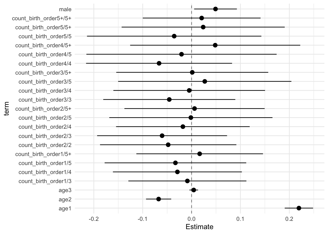
Model Comparison
anova(model_genes_m1, model_genes_m2, model_genes_m3, model_genes_m4)##
## Call:
##
## anova.mitml.result(object = model_genes_m1, model_genes_m2, model_genes_m3,
## model_genes_m4)
##
## Model comparison calculated from 50 imputed data sets.
## Combination method: D3
##
## Model 1: outcome~count_birth_order+poly(age,degree=3,raw=T)+male+(1|mother_pidlink)
## Model 2: outcome~birth_order_nonlinear+poly(age,degree=3,raw=T)+male+sibling_count+(1|mother_pidlink)
## Model 3: outcome~birth_order+poly(age,degree=3,raw=T)+male+sibling_count+(1|mother_pidlink)
## Model 4: outcome~poly(age,degree=3,raw=T)+male+sibling_count+(1|mother_pidlink)
##
## F.value df1 df2 P(>F) RIV
## 1 vs 2: 0.325 10 2672.812 0.975 0.741
## 2 vs 3: 0.127 4 1041.492 0.973 0.747
## 3 vs 4: 0.122 1 221.312 0.728 0.801Agreeableness
# Specify your outcome
data_used = data_used %>% mutate(outcome = big5_agree)
data_used_plots <- data_used[[1]]

compare_birthorder_imputed(data_used = data_used)
Parental full sibling order
Basic Model
# with.mitml.list <- function (data, expr, ...)
# {
#     expr <- substitute(expr)
#     parent <- parent.frame()
#     out <- parallel::mclapply(data, function(x) eval(expr, x, parent))
#     class(out) <- c("mitml.result", "list")
#     out
# }
Model Summary
data_used = data_used %>%
  mutate(sibling_count = sibling_count_genes_factor,
         birth_order_nonlinear = birthorder_genes_factor,
         birth_order = birthorder_genes,
         count_birth_order = count_birthorder_genes)

data_used_plots = data_used[[1]]

model_genes_m1 <- with(data_used, lmer(outcome ~ poly(age, degree = 3, raw = T)+ male + sibling_count + (1 | mother_pidlink), REML = FALSE))
x = mitml::testEstimates(model_genes_m1, var.comp = T)

y = as_tibble(x$estimates, rownames = "id")

y = y %>%
  mutate(CI_low = Estimate - 2.576 * Std.Error,
         CI_high = Estimate + 2.576 * Std.Error) %>%
  select(CI_low, CI_high)
CI_low = y$CI_low
CI_high = y$CI_high


x$estimates = cbind(x$estimates[,1:2], CI_low, CI_high, x$estimates[,3:7])
x
##
## Call:
##
## mitml::testEstimates(model = model_genes_m1, var.comp = T)
##
## Final parameter estimates and inferences obtained from 50 imputed data sets.
##
## Estimate Std.Error CI_low CI_high t.value df P(>|t|) RIV FMI
## (Intercept) -0.002 0.029 -0.076 0.073 -0.055 657.704 0.956 0.375 0.275
## poly(age, degree = 3, raw = T)1 0.096 0.011 0.067 0.125 8.502 8122.250 0.000 0.084 0.078
## poly(age, degree = 3, raw = T)2 -0.030 0.010 -0.055 -0.004 -2.959 4277.975 0.003 0.120 0.107
## poly(age, degree = 3, raw = T)3 -0.000 0.003 -0.009 0.008 -0.138 12785.531 0.891 0.066 0.062
## male 0.057 0.017 0.014 0.101 3.376 2203.191 0.001 0.175 0.150
## sibling_count3 -0.010 0.034 -0.097 0.077 -0.300 527.111 0.764 0.439 0.308
## sibling_count4 -0.005 0.035 -0.096 0.086 -0.139 392.097 0.890 0.547 0.357
## sibling_count5 0.032 0.038 -0.066 0.130 0.848 357.287 0.397 0.588 0.374
## sibling_count5+ 0.003 0.032 -0.078 0.085 0.102 595.465 0.918 0.402 0.289
##
## Estimate
## Intercept~~Intercept|mother_pidlink 0.068
## Residual~~Residual 0.923
## ICC|mother_pidlink 0.069
##
## Unadjusted hypothesis test as appropriate in larger samples.x$estimates %>%
as.data.frame() %>%
tibble::rownames_to_column("term") %>%
filter(term != "(Intercept)") %>%
mutate(term = str_replace_all(term, "poly\\(", "")) %>%
mutate(term = str_replace_all(term, ", degree = 3, raw = T\\)", "")) %>%
ggplot(aes(x= term, y = Estimate, ymin = CI_low, ymax = CI_high)) +
geom_hline(yintercept = 0, linetype = "dashed", alpha = 0.5) +
geom_pointrange() +
coord_flip() +
theme_minimal()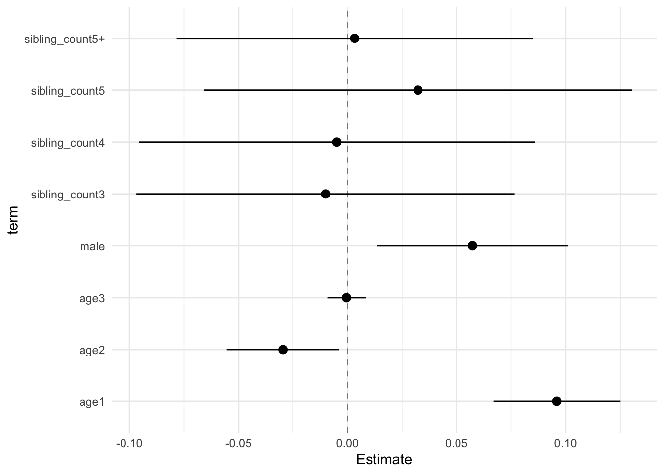
Add Birth Order Linear
Model Summary
model_genes_m2 <- with(data_used, lmer(outcome ~ birth_order + poly(age, degree = 3, raw = T)+ male + sibling_count +
                                         (1 | mother_pidlink), REML = FALSE))
x = mitml::testEstimates(model_genes_m2, var.comp = T)

y = as_tibble(x$estimates, rownames = "id")

y = y %>%
  mutate(CI_low = Estimate - 2.576 * Std.Error,
         CI_high = Estimate + 2.576 * Std.Error) %>%
  select(CI_low, CI_high)
CI_low = y$CI_low
CI_high = y$CI_high


x$estimates = cbind(x$estimates[,1:2], CI_low, CI_high, x$estimates[,3:7])
x
##
## Call:
##
## mitml::testEstimates(model = model_genes_m2, var.comp = T)
##
## Final parameter estimates and inferences obtained from 50 imputed data sets.
##
## Estimate Std.Error CI_low CI_high t.value df P(>|t|) RIV FMI
## (Intercept) -0.001 0.029 -0.077 0.075 -0.037 747.246 0.970 0.344 0.258
## birth_order -0.000 0.006 -0.015 0.014 -0.068 635.750 0.946 0.384 0.280
## poly(age, degree = 3, raw = T)1 0.096 0.011 0.067 0.125 8.488 9494.112 0.000 0.077 0.072
## poly(age, degree = 3, raw = T)2 -0.030 0.010 -0.055 -0.004 -2.960 4329.944 0.003 0.119 0.107
## poly(age, degree = 3, raw = T)3 -0.000 0.003 -0.009 0.008 -0.135 13190.506 0.893 0.065 0.061
## male 0.057 0.017 0.014 0.101 3.377 2210.522 0.001 0.175 0.150
## sibling_count3 -0.010 0.034 -0.097 0.077 -0.294 524.520 0.769 0.440 0.308
## sibling_count4 -0.005 0.036 -0.097 0.088 -0.127 376.461 0.899 0.564 0.364
## sibling_count5 0.033 0.039 -0.068 0.134 0.838 343.555 0.403 0.607 0.381
## sibling_count5+ 0.004 0.035 -0.087 0.095 0.118 491.948 0.906 0.461 0.318
##
## Estimate
## Intercept~~Intercept|mother_pidlink 0.068
## Residual~~Residual 0.923
## ICC|mother_pidlink 0.069
##
## Unadjusted hypothesis test as appropriate in larger samples.x$estimates %>%
as.data.frame() %>%
tibble::rownames_to_column("term") %>%
filter(term != "(Intercept)") %>%
mutate(term = str_replace_all(term, "poly\\(", "")) %>%
mutate(term = str_replace_all(term, ", degree = 3, raw = T\\)", "")) %>%
ggplot(aes(x= term, y = Estimate, ymin = CI_low, ymax = CI_high)) +
geom_hline(yintercept = 0, linetype = "dashed", alpha = 0.5) +
geom_pointrange() +
coord_flip() +
theme_minimal()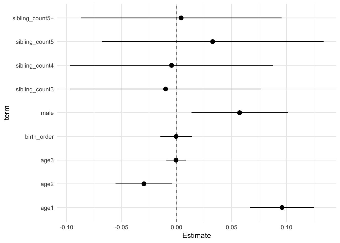
Add Birth Order Factor
Model Summary
model_genes_m3 <- with(data_used, lmer(outcome ~ birth_order_nonlinear + poly(age, degree = 3, raw = T)+ male + sibling_count +
                                         (1 | mother_pidlink), REML = FALSE))
x = mitml::testEstimates(model_genes_m3, var.comp = T)

y = as_tibble(x$estimates, rownames = "id")

y = y %>%
  mutate(CI_low = Estimate - 2.576 * Std.Error,
         CI_high = Estimate + 2.576 * Std.Error) %>%
  select(CI_low, CI_high)
CI_low = y$CI_low
CI_high = y$CI_high


x$estimates = cbind(x$estimates[,1:2], CI_low, CI_high, x$estimates[,3:7])
x
##
## Call:
##
## mitml::testEstimates(model = model_genes_m3, var.comp = T)
##
## Final parameter estimates and inferences obtained from 50 imputed data sets.
##
## Estimate Std.Error CI_low CI_high t.value df P(>|t|) RIV FMI
## (Intercept) 0.002 0.030 -0.076 0.080 0.063 618.704 0.949 0.392 0.284
## birth_order_nonlinear2 -0.010 0.026 -0.076 0.056 -0.385 342.719 0.701 0.608 0.382
## birth_order_nonlinear3 -0.019 0.030 -0.097 0.060 -0.609 392.033 0.543 0.547 0.357
## birth_order_nonlinear4 0.000 0.039 -0.100 0.101 0.010 286.350 0.992 0.706 0.418
## birth_order_nonlinear5 0.003 0.046 -0.114 0.121 0.076 580.959 0.940 0.409 0.293
## birth_order_nonlinear5+ -0.001 0.042 -0.110 0.108 -0.029 520.013 0.977 0.443 0.310
## poly(age, degree = 3, raw = T)1 0.096 0.011 0.067 0.125 8.500 9023.017 0.000 0.080 0.074
## poly(age, degree = 3, raw = T)2 -0.030 0.010 -0.055 -0.004 -2.955 4296.194 0.003 0.120 0.107
## poly(age, degree = 3, raw = T)3 -0.000 0.003 -0.009 0.008 -0.143 12873.798 0.886 0.066 0.062
## male 0.057 0.017 0.014 0.101 3.372 2164.217 0.001 0.177 0.151
## sibling_count3 -0.006 0.034 -0.095 0.083 -0.178 513.426 0.858 0.447 0.312
## sibling_count4 -0.002 0.037 -0.098 0.093 -0.067 355.585 0.947 0.590 0.375
## sibling_count5 0.033 0.040 -0.069 0.135 0.841 382.438 0.401 0.558 0.361
## sibling_count5+ 0.004 0.036 -0.089 0.096 0.106 480.348 0.916 0.469 0.322
##
## Estimate
## Intercept~~Intercept|mother_pidlink 0.069
## Residual~~Residual 0.922
## ICC|mother_pidlink 0.069
##
## Unadjusted hypothesis test as appropriate in larger samples.x$estimates %>%
as.data.frame() %>%
tibble::rownames_to_column("term") %>%
filter(term != "(Intercept)") %>%
mutate(term = str_replace_all(term, "poly\\(", "")) %>%
mutate(term = str_replace_all(term, ", degree = 3, raw = T\\)", "")) %>%
ggplot(aes(x= term, y = Estimate, ymin = CI_low, ymax = CI_high)) +
geom_hline(yintercept = 0, linetype = "dashed", alpha = 0.5) +
geom_pointrange() +
coord_flip() +
theme_minimal()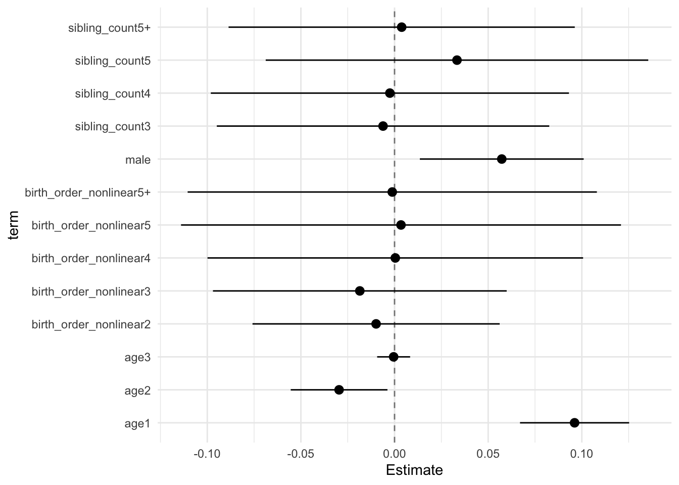
Add Interaction
Model Summary
model_genes_m4 <- with(data_used, lmer(outcome ~ count_birth_order + poly(age, degree = 3, raw = T)+ male  +
                                         (1 | mother_pidlink), REML = FALSE))
x = mitml::testEstimates(model_genes_m4, var.comp = T)

y = as_tibble(x$estimates, rownames = "id")

y = y %>%
  mutate(CI_low = Estimate - 2.576 * Std.Error,
         CI_high = Estimate + 2.576 * Std.Error) %>%
  select(CI_low, CI_high)
CI_low = y$CI_low
CI_high = y$CI_high


x$estimates = cbind(x$estimates[,1:2], CI_low, CI_high, x$estimates[,3:7])
x
##
## Call:
##
## mitml::testEstimates(model = model_genes_m4, var.comp = T)
##
## Final parameter estimates and inferences obtained from 50 imputed data sets.
##
## Estimate Std.Error CI_low CI_high t.value df P(>|t|) RIV FMI
## (Intercept) 0.003 0.035 -0.086 0.092 0.097 537.449 0.923 0.433 0.305
## count_birth_order2/2 -0.014 0.052 -0.148 0.120 -0.271 439.591 0.787 0.501 0.337
## count_birth_order1/3 -0.001 0.046 -0.120 0.119 -0.015 380.794 0.988 0.559 0.362
## count_birth_order2/3 -0.016 0.053 -0.153 0.122 -0.290 309.383 0.772 0.661 0.402
## count_birth_order3/3 -0.041 0.053 -0.179 0.096 -0.778 508.055 0.437 0.450 0.313
## count_birth_order1/4 -0.003 0.050 -0.130 0.125 -0.059 396.204 0.953 0.542 0.355
## count_birth_order2/4 -0.021 0.055 -0.162 0.120 -0.388 362.479 0.698 0.581 0.371
## count_birth_order3/4 -0.022 0.061 -0.179 0.136 -0.353 353.932 0.724 0.593 0.376
## count_birth_order4/4 0.003 0.060 -0.152 0.158 0.054 326.745 0.957 0.632 0.391
## count_birth_order1/5 0.012 0.058 -0.138 0.162 0.211 290.602 0.833 0.697 0.415
## count_birth_order2/5 0.024 0.062 -0.137 0.184 0.379 448.692 0.705 0.494 0.333
## count_birth_order3/5 0.029 0.078 -0.172 0.230 0.371 199.270 0.711 0.984 0.501
## count_birth_order4/5 0.002 0.079 -0.202 0.206 0.031 268.714 0.975 0.745 0.431
## count_birth_order5/5 0.080 0.071 -0.102 0.262 1.129 342.717 0.260 0.608 0.382
## count_birth_order1/5+ 0.004 0.050 -0.124 0.132 0.080 427.901 0.936 0.511 0.341
## count_birth_order2/5+ -0.001 0.056 -0.145 0.143 -0.016 331.861 0.987 0.624 0.388
## count_birth_order3/5+ -0.009 0.058 -0.158 0.140 -0.155 479.751 0.877 0.470 0.322
## count_birth_order4/5+ 0.014 0.066 -0.156 0.183 0.208 293.610 0.835 0.691 0.413
## count_birth_order5/5+ -0.036 0.067 -0.209 0.138 -0.528 411.629 0.598 0.527 0.348
## count_birth_order5+/5+ 0.001 0.046 -0.118 0.119 0.018 624.179 0.986 0.389 0.282
## poly(age, degree = 3, raw = T)1 0.096 0.011 0.067 0.125 8.540 10710.641 0.000 0.073 0.068
## poly(age, degree = 3, raw = T)2 -0.030 0.010 -0.055 -0.004 -2.954 4283.480 0.003 0.120 0.107
## poly(age, degree = 3, raw = T)3 -0.001 0.003 -0.009 0.008 -0.151 13543.190 0.880 0.064 0.060
## male 0.057 0.017 0.014 0.101 3.377 2109.704 0.001 0.180 0.153
##
## Estimate
## Intercept~~Intercept|mother_pidlink 0.069
## Residual~~Residual 0.922
## ICC|mother_pidlink 0.069
##
## Unadjusted hypothesis test as appropriate in larger samples.x$estimates %>%
as.data.frame() %>%
tibble::rownames_to_column("term") %>%
filter(term != "(Intercept)") %>%
mutate(term = str_replace_all(term, "poly\\(", "")) %>%
mutate(term = str_replace_all(term, ", degree = 3, raw = T\\)", "")) %>%
ggplot(aes(x= term, y = Estimate, ymin = CI_low, ymax = CI_high)) +
geom_hline(yintercept = 0, linetype = "dashed", alpha = 0.5) +
geom_pointrange() +
coord_flip() +
theme_minimal()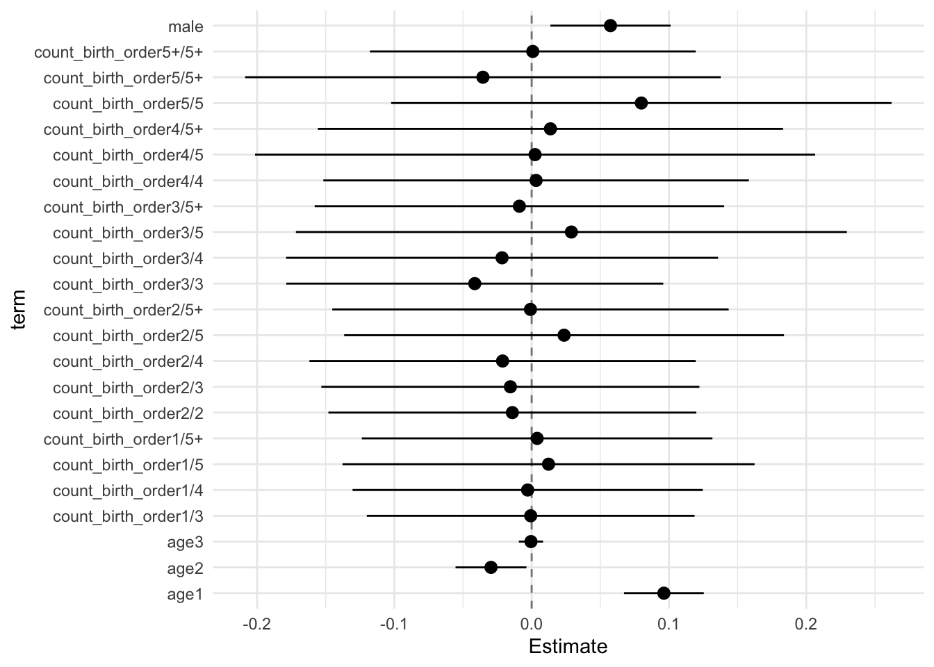
Model Comparison
anova(model_genes_m1, model_genes_m2, model_genes_m3, model_genes_m4)##
## Call:
##
## anova.mitml.result(object = model_genes_m1, model_genes_m2, model_genes_m3,
## model_genes_m4)
##
## Model comparison calculated from 50 imputed data sets.
## Combination method: D3
##
## Model 1: outcome~count_birth_order+poly(age,degree=3,raw=T)+male+(1|mother_pidlink)
## Model 2: outcome~birth_order_nonlinear+poly(age,degree=3,raw=T)+male+sibling_count+(1|mother_pidlink)
## Model 3: outcome~birth_order+poly(age,degree=3,raw=T)+male+sibling_count+(1|mother_pidlink)
## Model 4: outcome~poly(age,degree=3,raw=T)+male+sibling_count+(1|mother_pidlink)
##
## F.value df1 df2 P(>F) RIV
## 1 vs 2: 0.164 10 2782.083 0.998 0.716
## 2 vs 3: 0.124 4 1326.531 0.974 0.609
## 3 vs 4: 0.005 1 552.901 0.946 0.385Openness
# Specify your outcome
data_used = data_used %>% mutate(outcome = big5_open)
data_used_plots <- data_used[[1]]

compare_birthorder_imputed(data_used = data_used)
Parental full sibling order
Basic Model
# with.mitml.list <- function (data, expr, ...)
# {
#     expr <- substitute(expr)
#     parent <- parent.frame()
#     out <- parallel::mclapply(data, function(x) eval(expr, x, parent))
#     class(out) <- c("mitml.result", "list")
#     out
# }
Model Summary
data_used = data_used %>%
  mutate(sibling_count = sibling_count_genes_factor,
         birth_order_nonlinear = birthorder_genes_factor,
         birth_order = birthorder_genes,
         count_birth_order = count_birthorder_genes)

data_used_plots = data_used[[1]]

model_genes_m1 <- with(data_used, lmer(outcome ~ poly(age, degree = 3, raw = T)+ male + sibling_count + (1 | mother_pidlink), REML = FALSE))
x = mitml::testEstimates(model_genes_m1, var.comp = T)

y = as_tibble(x$estimates, rownames = "id")

y = y %>%
  mutate(CI_low = Estimate - 2.576 * Std.Error,
         CI_high = Estimate + 2.576 * Std.Error) %>%
  select(CI_low, CI_high)
CI_low = y$CI_low
CI_high = y$CI_high


x$estimates = cbind(x$estimates[,1:2], CI_low, CI_high, x$estimates[,3:7])
x
##
## Call:
##
## mitml::testEstimates(model = model_genes_m1, var.comp = T)
##
## Final parameter estimates and inferences obtained from 50 imputed data sets.
##
## Estimate Std.Error CI_low CI_high t.value df P(>|t|) RIV FMI
## (Intercept) -0.042 0.029 -0.118 0.034 -1.427 571.298 0.154 0.414 0.295
## poly(age, degree = 3, raw = T)1 -0.008 0.011 -0.037 0.021 -0.701 6741.798 0.483 0.093 0.086
## poly(age, degree = 3, raw = T)2 0.021 0.010 -0.006 0.047 2.034 2818.803 0.042 0.152 0.132
## poly(age, degree = 3, raw = T)3 -0.010 0.003 -0.019 -0.001 -2.879 7932.934 0.004 0.085 0.079
## male 0.166 0.017 0.122 0.210 9.648 1588.972 0.000 0.213 0.177
## sibling_count3 -0.047 0.036 -0.139 0.046 -1.298 337.144 0.195 0.616 0.385
## sibling_count4 -0.044 0.036 -0.137 0.048 -1.231 353.407 0.219 0.593 0.376
## sibling_count5 -0.073 0.039 -0.172 0.027 -1.880 339.283 0.061 0.613 0.384
## sibling_count5+ -0.087 0.034 -0.174 -0.000 -2.587 374.182 0.010 0.567 0.365
##
## Estimate
## Intercept~~Intercept|mother_pidlink 0.079
## Residual~~Residual 0.911
## ICC|mother_pidlink 0.080
##
## Unadjusted hypothesis test as appropriate in larger samples.x$estimates %>%
as.data.frame() %>%
tibble::rownames_to_column("term") %>%
filter(term != "(Intercept)") %>%
mutate(term = str_replace_all(term, "poly\\(", "")) %>%
mutate(term = str_replace_all(term, ", degree = 3, raw = T\\)", "")) %>%
ggplot(aes(x= term, y = Estimate, ymin = CI_low, ymax = CI_high)) +
geom_hline(yintercept = 0, linetype = "dashed", alpha = 0.5) +
geom_pointrange() +
coord_flip() +
theme_minimal()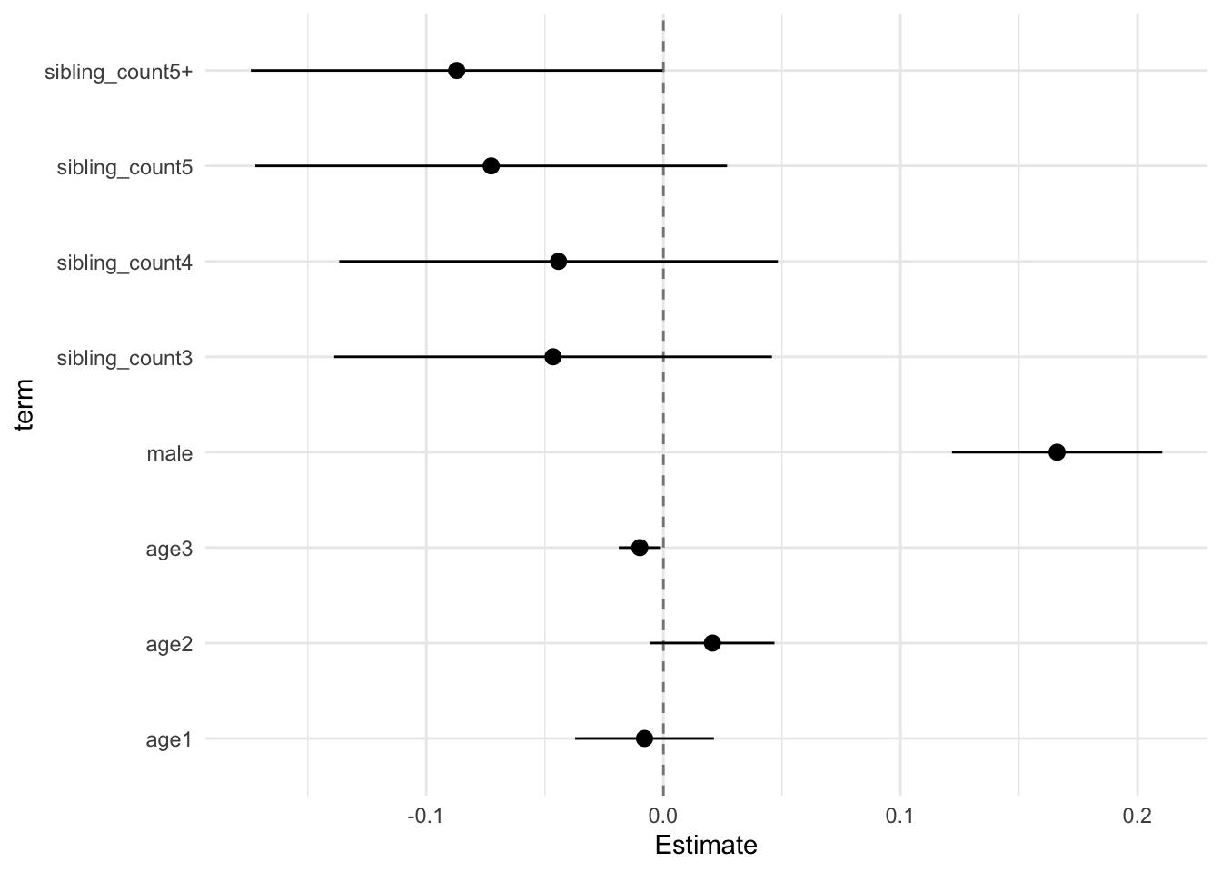
Add Birth Order Linear
Model Summary
model_genes_m2 <- with(data_used, lmer(outcome ~ birth_order + poly(age, degree = 3, raw = T)+ male + sibling_count +
                                         (1 | mother_pidlink), REML = FALSE))
x = mitml::testEstimates(model_genes_m2, var.comp = T)

y = as_tibble(x$estimates, rownames = "id")

y = y %>%
  mutate(CI_low = Estimate - 2.576 * Std.Error,
         CI_high = Estimate + 2.576 * Std.Error) %>%
  select(CI_low, CI_high)
CI_low = y$CI_low
CI_high = y$CI_high


x$estimates = cbind(x$estimates[,1:2], CI_low, CI_high, x$estimates[,3:7])
x
##
## Call:
##
## mitml::testEstimates(model = model_genes_m2, var.comp = T)
##
## Final parameter estimates and inferences obtained from 50 imputed data sets.
##
## Estimate Std.Error CI_low CI_high t.value df P(>|t|) RIV FMI
## (Intercept) -0.047 0.030 -0.124 0.029 -1.589 663.423 0.113 0.373 0.274
## birth_order 0.004 0.006 -0.011 0.019 0.714 435.825 0.476 0.504 0.338
## poly(age, degree = 3, raw = T)1 -0.007 0.011 -0.037 0.022 -0.622 6557.395 0.534 0.095 0.087
## poly(age, degree = 3, raw = T)2 0.021 0.010 -0.005 0.047 2.054 2807.489 0.040 0.152 0.133
## poly(age, degree = 3, raw = T)3 -0.010 0.003 -0.019 -0.001 -2.904 7881.215 0.004 0.086 0.079
## male 0.166 0.017 0.122 0.210 9.651 1590.273 0.000 0.213 0.177
## sibling_count3 -0.048 0.036 -0.141 0.045 -1.341 327.731 0.181 0.630 0.390
## sibling_count4 -0.048 0.036 -0.142 0.046 -1.320 347.992 0.188 0.601 0.379
## sibling_count5 -0.078 0.039 -0.180 0.024 -1.979 336.942 0.049 0.616 0.385
## sibling_count5+ -0.098 0.038 -0.195 -0.000 -2.587 320.606 0.010 0.642 0.395
##
## Estimate
## Intercept~~Intercept|mother_pidlink 0.079
## Residual~~Residual 0.911
## ICC|mother_pidlink 0.080
##
## Unadjusted hypothesis test as appropriate in larger samples.x$estimates %>%
as.data.frame() %>%
tibble::rownames_to_column("term") %>%
filter(term != "(Intercept)") %>%
mutate(term = str_replace_all(term, "poly\\(", "")) %>%
mutate(term = str_replace_all(term, ", degree = 3, raw = T\\)", "")) %>%
ggplot(aes(x= term, y = Estimate, ymin = CI_low, ymax = CI_high)) +
geom_hline(yintercept = 0, linetype = "dashed", alpha = 0.5) +
geom_pointrange() +
coord_flip() +
theme_minimal()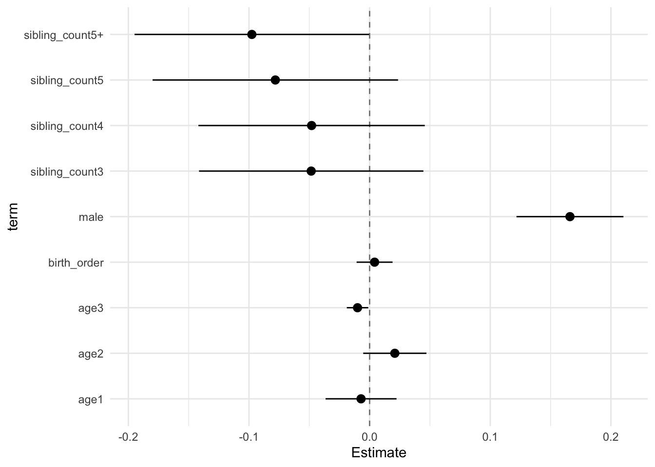
Add Birth Order Factor
Model Summary
model_genes_m3 <- with(data_used, lmer(outcome ~ birth_order_nonlinear + poly(age, degree = 3, raw = T)+ male + sibling_count +
                                         (1 | mother_pidlink), REML = FALSE))
x = mitml::testEstimates(model_genes_m3, var.comp = T)

y = as_tibble(x$estimates, rownames = "id")

y = y %>%
  mutate(CI_low = Estimate - 2.576 * Std.Error,
         CI_high = Estimate + 2.576 * Std.Error) %>%
  select(CI_low, CI_high)
CI_low = y$CI_low
CI_high = y$CI_high


x$estimates = cbind(x$estimates[,1:2], CI_low, CI_high, x$estimates[,3:7])
x
##
## Call:
##
## mitml::testEstimates(model = model_genes_m3, var.comp = T)
##
## Final parameter estimates and inferences obtained from 50 imputed data sets.
##
## Estimate Std.Error CI_low CI_high t.value df P(>|t|) RIV FMI
## (Intercept) -0.045 0.032 -0.126 0.037 -1.405 410.314 0.161 0.528 0.349
## birth_order_nonlinear2 0.008 0.027 -0.063 0.079 0.287 230.242 0.774 0.856 0.466
## birth_order_nonlinear3 0.012 0.030 -0.065 0.090 0.410 409.864 0.682 0.528 0.349
## birth_order_nonlinear4 0.022 0.042 -0.085 0.130 0.540 205.137 0.590 0.956 0.494
## birth_order_nonlinear5 0.041 0.047 -0.080 0.163 0.873 424.415 0.383 0.515 0.343
## birth_order_nonlinear5+ 0.011 0.042 -0.098 0.120 0.267 536.766 0.789 0.433 0.305
## poly(age, degree = 3, raw = T)1 -0.007 0.011 -0.037 0.022 -0.637 6296.097 0.524 0.097 0.089
## poly(age, degree = 3, raw = T)2 0.021 0.010 -0.005 0.047 2.048 2798.978 0.041 0.152 0.133
## poly(age, degree = 3, raw = T)3 -0.010 0.003 -0.019 -0.001 -2.894 7738.945 0.004 0.086 0.080
## male 0.166 0.017 0.122 0.210 9.643 1582.342 0.000 0.214 0.177
## sibling_count3 -0.049 0.037 -0.144 0.046 -1.333 315.964 0.183 0.650 0.398
## sibling_count4 -0.051 0.038 -0.147 0.046 -1.342 334.353 0.181 0.620 0.386
## sibling_count5 -0.084 0.041 -0.188 0.021 -2.058 333.598 0.040 0.621 0.387
## sibling_count5+ -0.097 0.038 -0.195 0.001 -2.540 320.935 0.012 0.641 0.395
##
## Estimate
## Intercept~~Intercept|mother_pidlink 0.079
## Residual~~Residual 0.911
## ICC|mother_pidlink 0.080
##
## Unadjusted hypothesis test as appropriate in larger samples.x$estimates %>%
as.data.frame() %>%
tibble::rownames_to_column("term") %>%
filter(term != "(Intercept)") %>%
mutate(term = str_replace_all(term, "poly\\(", "")) %>%
mutate(term = str_replace_all(term, ", degree = 3, raw = T\\)", "")) %>%
ggplot(aes(x= term, y = Estimate, ymin = CI_low, ymax = CI_high)) +
geom_hline(yintercept = 0, linetype = "dashed", alpha = 0.5) +
geom_pointrange() +
coord_flip() +
theme_minimal()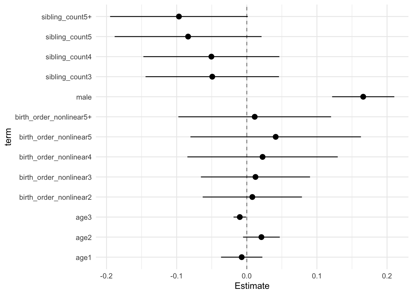
Add Interaction
Model Summary
model_genes_m4 <- with(data_used, lmer(outcome ~ count_birth_order + poly(age, degree = 3, raw = T)+ male  +
                                         (1 | mother_pidlink), REML = FALSE))
x = mitml::testEstimates(model_genes_m4, var.comp = T)

y = as_tibble(x$estimates, rownames = "id")

y = y %>%
  mutate(CI_low = Estimate - 2.576 * Std.Error,
         CI_high = Estimate + 2.576 * Std.Error) %>%
  select(CI_low, CI_high)
CI_low = y$CI_low
CI_high = y$CI_high


x$estimates = cbind(x$estimates[,1:2], CI_low, CI_high, x$estimates[,3:7])
x
##
## Call:
##
## mitml::testEstimates(model = model_genes_m4, var.comp = T)
##
## Final parameter estimates and inferences obtained from 50 imputed data sets.
##
## Estimate Std.Error CI_low CI_high t.value df P(>|t|) RIV FMI
## (Intercept) -0.038 0.037 -0.132 0.057 -1.031 341.681 0.303 0.610 0.382
## count_birth_order2/2 -0.012 0.056 -0.157 0.133 -0.208 260.553 0.836 0.766 0.438
## count_birth_order1/3 -0.059 0.048 -0.182 0.064 -1.229 310.425 0.220 0.659 0.401
## count_birth_order2/3 -0.052 0.057 -0.199 0.096 -0.904 217.443 0.367 0.904 0.479
## count_birth_order3/3 -0.034 0.054 -0.174 0.105 -0.633 437.949 0.527 0.503 0.338
## count_birth_order1/4 -0.055 0.049 -0.181 0.071 -1.130 437.504 0.259 0.503 0.338
## count_birth_order2/4 -0.054 0.056 -0.197 0.090 -0.959 315.537 0.338 0.650 0.398
## count_birth_order3/4 -0.044 0.061 -0.201 0.114 -0.713 349.144 0.476 0.599 0.378
## count_birth_order4/4 -0.034 0.068 -0.210 0.141 -0.506 180.565 0.614 1.087 0.526
## count_birth_order1/5 -0.103 0.059 -0.256 0.050 -1.740 263.730 0.083 0.758 0.435
## count_birth_order2/5 -0.055 0.070 -0.235 0.124 -0.797 226.878 0.426 0.868 0.469
## count_birth_order3/5 -0.092 0.072 -0.278 0.094 -1.276 288.426 0.203 0.701 0.416
## count_birth_order4/5 -0.048 0.076 -0.244 0.148 -0.631 344.715 0.528 0.605 0.381
## count_birth_order5/5 -0.062 0.072 -0.248 0.124 -0.854 300.963 0.394 0.676 0.407
## count_birth_order1/5+ -0.103 0.055 -0.245 0.040 -1.853 224.414 0.065 0.877 0.472
## count_birth_order2/5+ -0.092 0.062 -0.253 0.068 -1.479 194.990 0.141 1.005 0.506
## count_birth_order3/5+ -0.095 0.061 -0.251 0.062 -1.561 338.764 0.119 0.614 0.384
## count_birth_order4/5+ -0.094 0.071 -0.277 0.088 -1.330 202.777 0.185 0.967 0.497
## count_birth_order5/5+ -0.050 0.068 -0.225 0.125 -0.741 382.053 0.459 0.558 0.361
## count_birth_order5+/5+ -0.092 0.050 -0.220 0.035 -1.861 344.567 0.064 0.605 0.381
## poly(age, degree = 3, raw = T)1 -0.007 0.011 -0.037 0.022 -0.637 5919.260 0.524 0.100 0.091
## poly(age, degree = 3, raw = T)2 0.021 0.010 -0.005 0.047 2.047 2806.341 0.041 0.152 0.133
## poly(age, degree = 3, raw = T)3 -0.010 0.003 -0.019 -0.001 -2.894 8032.382 0.004 0.085 0.078
## male 0.166 0.017 0.122 0.210 9.652 1606.892 0.000 0.212 0.176
##
## Estimate
## Intercept~~Intercept|mother_pidlink 0.079
## Residual~~Residual 0.911
## ICC|mother_pidlink 0.080
##
## Unadjusted hypothesis test as appropriate in larger samples.x$estimates %>%
as.data.frame() %>%
tibble::rownames_to_column("term") %>%
filter(term != "(Intercept)") %>%
mutate(term = str_replace_all(term, "poly\\(", "")) %>%
mutate(term = str_replace_all(term, ", degree = 3, raw = T\\)", "")) %>%
ggplot(aes(x= term, y = Estimate, ymin = CI_low, ymax = CI_high)) +
geom_hline(yintercept = 0, linetype = "dashed", alpha = 0.5) +
geom_pointrange() +
coord_flip() +
theme_minimal()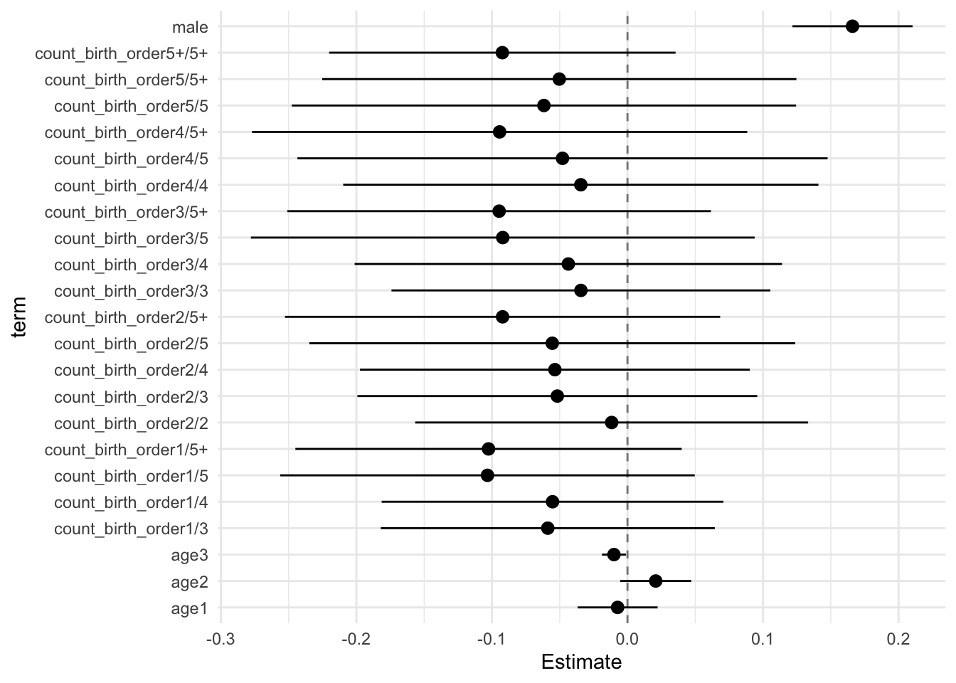
Model Comparison
anova(model_genes_m1, model_genes_m2, model_genes_m3, model_genes_m4)##
## Call:
##
## anova.mitml.result(object = model_genes_m1, model_genes_m2, model_genes_m3,
## model_genes_m4)
##
## Model comparison calculated from 50 imputed data sets.
## Combination method: D3
##
## Model 1: outcome~count_birth_order+poly(age,degree=3,raw=T)+male+(1|mother_pidlink)
## Model 2: outcome~birth_order_nonlinear+poly(age,degree=3,raw=T)+male+sibling_count+(1|mother_pidlink)
## Model 3: outcome~birth_order+poly(age,degree=3,raw=T)+male+sibling_count+(1|mother_pidlink)
## Model 4: outcome~poly(age,degree=3,raw=T)+male+sibling_count+(1|mother_pidlink)
##
## F.value df1 df2 P(>F) RIV
## 1 vs 2: 0.075 10 2524.085 1.000 0.780
## 2 vs 3: 0.104 4 1146.245 0.981 0.688
## 3 vs 4: 0.512 1 383.335 0.475 0.504Riskpreference
Risk A
# Specify your outcome
data_used = data_used %>% mutate(outcome = riskA)
data_used_plots <- data_used[[1]]

compare_birthorder_imputed(data_used = data_used)
Parental full sibling order
Basic Model
# with.mitml.list <- function (data, expr, ...)
# {
#     expr <- substitute(expr)
#     parent <- parent.frame()
#     out <- parallel::mclapply(data, function(x) eval(expr, x, parent))
#     class(out) <- c("mitml.result", "list")
#     out
# }
Model Summary
data_used = data_used %>%
  mutate(sibling_count = sibling_count_genes_factor,
         birth_order_nonlinear = birthorder_genes_factor,
         birth_order = birthorder_genes,
         count_birth_order = count_birthorder_genes)

data_used_plots = data_used[[1]]

model_genes_m1 <- with(data_used, lmer(outcome ~ poly(age, degree = 3, raw = T)+ male + sibling_count + (1 | mother_pidlink), REML = FALSE))
x = mitml::testEstimates(model_genes_m1, var.comp = T)

y = as_tibble(x$estimates, rownames = "id")

y = y %>%
  mutate(CI_low = Estimate - 2.576 * Std.Error,
         CI_high = Estimate + 2.576 * Std.Error) %>%
  select(CI_low, CI_high)
CI_low = y$CI_low
CI_high = y$CI_high


x$estimates = cbind(x$estimates[,1:2], CI_low, CI_high, x$estimates[,3:7])
x
##
## Call:
##
## mitml::testEstimates(model = model_genes_m1, var.comp = T)
##
## Final parameter estimates and inferences obtained from 50 imputed data sets.
##
## Estimate Std.Error CI_low CI_high t.value df P(>|t|) RIV FMI
## (Intercept) 0.037 0.029 -0.038 0.112 1.280 586.117 0.201 0.407 0.292
## poly(age, degree = 3, raw = T)1 -0.012 0.012 -0.044 0.020 -0.947 870.625 0.344 0.311 0.239
## poly(age, degree = 3, raw = T)2 0.062 0.011 0.035 0.090 5.857 1019.703 0.000 0.281 0.221
## poly(age, degree = 3, raw = T)3 -0.015 0.004 -0.025 -0.006 -4.029 747.168 0.000 0.344 0.258
## male -0.234 0.018 -0.280 -0.188 -13.192 934.531 0.000 0.297 0.231
## sibling_count3 -0.012 0.036 -0.104 0.080 -0.322 325.329 0.747 0.634 0.392
## sibling_count4 0.014 0.037 -0.081 0.110 0.384 276.261 0.701 0.728 0.425
## sibling_count5 0.040 0.038 -0.058 0.138 1.054 347.585 0.293 0.601 0.379
## sibling_count5+ 0.065 0.033 -0.020 0.150 1.971 402.055 0.049 0.536 0.352
##
## Estimate
## Intercept~~Intercept|mother_pidlink 0.068
## Residual~~Residual 0.915
## ICC|mother_pidlink 0.069
##
## Unadjusted hypothesis test as appropriate in larger samples.x$estimates %>%
as.data.frame() %>%
tibble::rownames_to_column("term") %>%
filter(term != "(Intercept)") %>%
mutate(term = str_replace_all(term, "poly\\(", "")) %>%
mutate(term = str_replace_all(term, ", degree = 3, raw = T\\)", "")) %>%
ggplot(aes(x= term, y = Estimate, ymin = CI_low, ymax = CI_high)) +
geom_hline(yintercept = 0, linetype = "dashed", alpha = 0.5) +
geom_pointrange() +
coord_flip() +
theme_minimal()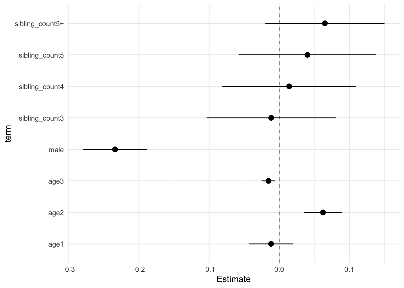
Add Birth Order Linear
Model Summary
model_genes_m2 <- with(data_used, lmer(outcome ~ birth_order + poly(age, degree = 3, raw = T)+ male + sibling_count +
                                         (1 | mother_pidlink), REML = FALSE))
x = mitml::testEstimates(model_genes_m2, var.comp = T)

y = as_tibble(x$estimates, rownames = "id")

y = y %>%
  mutate(CI_low = Estimate - 2.576 * Std.Error,
         CI_high = Estimate + 2.576 * Std.Error) %>%
  select(CI_low, CI_high)
CI_low = y$CI_low
CI_high = y$CI_high


x$estimates = cbind(x$estimates[,1:2], CI_low, CI_high, x$estimates[,3:7])
x
##
## Call:
##
## mitml::testEstimates(model = model_genes_m2, var.comp = T)
##
## Final parameter estimates and inferences obtained from 50 imputed data sets.
##
## Estimate Std.Error CI_low CI_high t.value df P(>|t|) RIV FMI
## (Intercept) 0.039 0.030 -0.038 0.116 1.312 638.823 0.190 0.383 0.279
## birth_order -0.001 0.006 -0.018 0.015 -0.214 237.632 0.830 0.832 0.459
## poly(age, degree = 3, raw = T)1 -0.012 0.012 -0.044 0.020 -0.965 858.486 0.335 0.314 0.241
## poly(age, degree = 3, raw = T)2 0.062 0.011 0.035 0.090 5.862 1058.560 0.000 0.274 0.217
## poly(age, degree = 3, raw = T)3 -0.015 0.004 -0.025 -0.006 -4.026 763.889 0.000 0.339 0.255
## male -0.234 0.018 -0.280 -0.188 -13.198 941.001 0.000 0.296 0.230
## sibling_count3 -0.011 0.036 -0.103 0.081 -0.304 323.138 0.761 0.638 0.393
## sibling_count4 0.015 0.038 -0.082 0.113 0.410 265.149 0.682 0.754 0.434
## sibling_count5 0.042 0.039 -0.059 0.143 1.070 329.142 0.286 0.628 0.390
## sibling_count5+ 0.069 0.038 -0.029 0.166 1.803 290.727 0.072 0.696 0.415
##
## Estimate
## Intercept~~Intercept|mother_pidlink 0.068
## Residual~~Residual 0.915
## ICC|mother_pidlink 0.069
##
## Unadjusted hypothesis test as appropriate in larger samples.x$estimates %>%
as.data.frame() %>%
tibble::rownames_to_column("term") %>%
filter(term != "(Intercept)") %>%
mutate(term = str_replace_all(term, "poly\\(", "")) %>%
mutate(term = str_replace_all(term, ", degree = 3, raw = T\\)", "")) %>%
ggplot(aes(x= term, y = Estimate, ymin = CI_low, ymax = CI_high)) +
geom_hline(yintercept = 0, linetype = "dashed", alpha = 0.5) +
geom_pointrange() +
coord_flip() +
theme_minimal()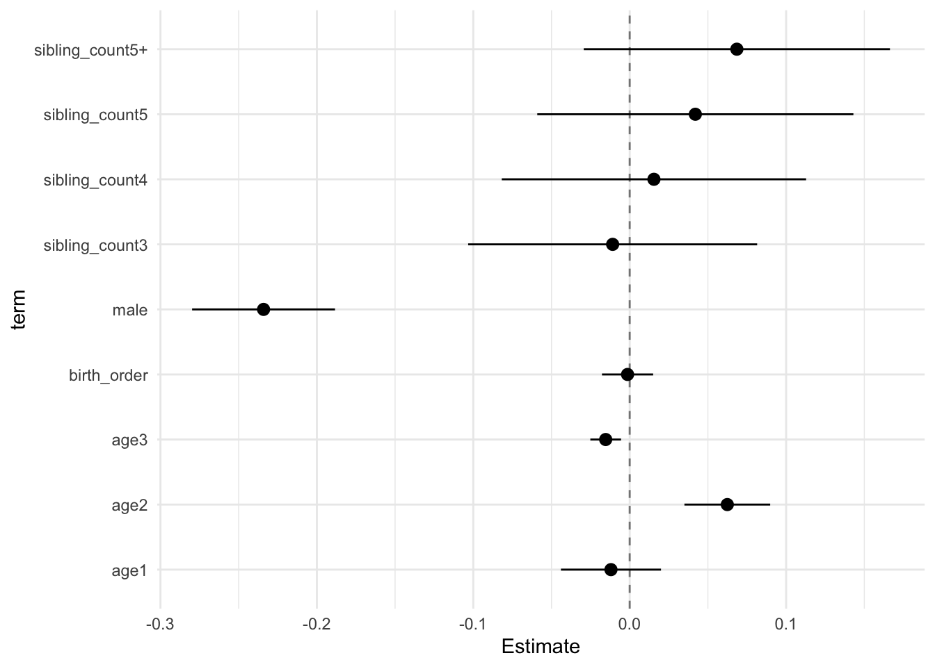
Add Birth Order Factor
Model Summary
model_genes_m3 <- with(data_used, lmer(outcome ~ birth_order_nonlinear + poly(age, degree = 3, raw = T)+ male + sibling_count +
                                         (1 | mother_pidlink), REML = FALSE))
x = mitml::testEstimates(model_genes_m3, var.comp = T)

y = as_tibble(x$estimates, rownames = "id")

y = y %>%
  mutate(CI_low = Estimate - 2.576 * Std.Error,
         CI_high = Estimate + 2.576 * Std.Error) %>%
  select(CI_low, CI_high)
CI_low = y$CI_low
CI_high = y$CI_high


x$estimates = cbind(x$estimates[,1:2], CI_low, CI_high, x$estimates[,3:7])
x
##
## Call:
##
## mitml::testEstimates(model = model_genes_m3, var.comp = T)
##
## Final parameter estimates and inferences obtained from 50 imputed data sets.
##
## Estimate Std.Error CI_low CI_high t.value df P(>|t|) RIV FMI
## (Intercept) 0.038 0.030 -0.039 0.114 1.258 687.022 0.209 0.364 0.269
## birth_order_nonlinear2 -0.001 0.027 -0.071 0.069 -0.031 245.549 0.975 0.807 0.451
## birth_order_nonlinear3 0.003 0.030 -0.073 0.079 0.100 466.860 0.920 0.479 0.327
## birth_order_nonlinear4 -0.014 0.038 -0.111 0.084 -0.360 324.653 0.719 0.635 0.392
## birth_order_nonlinear5 0.003 0.048 -0.121 0.127 0.068 356.358 0.946 0.589 0.374
## birth_order_nonlinear5+ 0.001 0.049 -0.124 0.126 0.027 217.053 0.978 0.905 0.480
## poly(age, degree = 3, raw = T)1 -0.012 0.012 -0.044 0.020 -0.944 829.852 0.346 0.321 0.245
## poly(age, degree = 3, raw = T)2 0.062 0.011 0.035 0.090 5.872 1068.053 0.000 0.273 0.216
## poly(age, degree = 3, raw = T)3 -0.015 0.004 -0.025 -0.006 -4.029 759.369 0.000 0.341 0.256
## male -0.234 0.018 -0.280 -0.188 -13.194 938.696 0.000 0.296 0.230
## sibling_count3 -0.012 0.036 -0.106 0.081 -0.338 334.702 0.735 0.620 0.386
## sibling_count4 0.016 0.038 -0.082 0.115 0.430 290.598 0.668 0.697 0.415
## sibling_count5 0.041 0.040 -0.061 0.143 1.031 370.887 0.303 0.571 0.367
## sibling_count5+ 0.065 0.038 -0.033 0.164 1.705 292.105 0.089 0.694 0.414
##
## Estimate
## Intercept~~Intercept|mother_pidlink 0.068
## Residual~~Residual 0.915
## ICC|mother_pidlink 0.069
##
## Unadjusted hypothesis test as appropriate in larger samples.x$estimates %>%
as.data.frame() %>%
tibble::rownames_to_column("term") %>%
filter(term != "(Intercept)") %>%
mutate(term = str_replace_all(term, "poly\\(", "")) %>%
mutate(term = str_replace_all(term, ", degree = 3, raw = T\\)", "")) %>%
ggplot(aes(x= term, y = Estimate, ymin = CI_low, ymax = CI_high)) +
geom_hline(yintercept = 0, linetype = "dashed", alpha = 0.5) +
geom_pointrange() +
coord_flip() +
theme_minimal()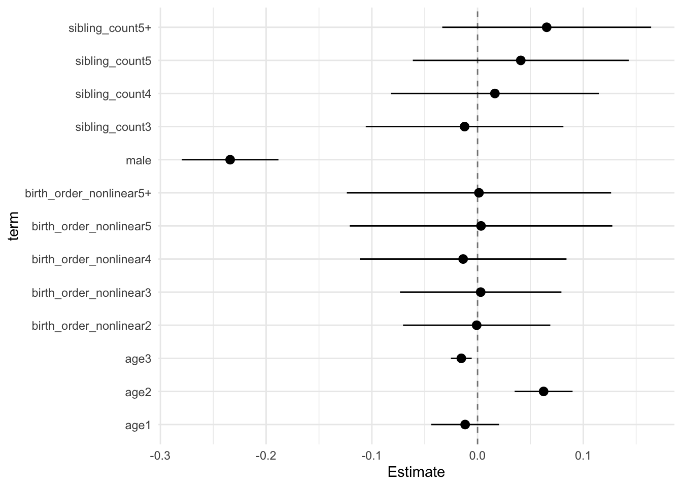
Add Interaction
Model Summary
model_genes_m4 <- with(data_used, lmer(outcome ~ count_birth_order + poly(age, degree = 3, raw = T)+ male  +
                                         (1 | mother_pidlink), REML = FALSE))
x = mitml::testEstimates(model_genes_m4, var.comp = T)

y = as_tibble(x$estimates, rownames = "id")

y = y %>%
  mutate(CI_low = Estimate - 2.576 * Std.Error,
         CI_high = Estimate + 2.576 * Std.Error) %>%
  select(CI_low, CI_high)
CI_low = y$CI_low
CI_high = y$CI_high


x$estimates = cbind(x$estimates[,1:2], CI_low, CI_high, x$estimates[,3:7])
x
##
## Call:
##
## mitml::testEstimates(model = model_genes_m4, var.comp = T)
##
## Final parameter estimates and inferences obtained from 50 imputed data sets.
##
## Estimate Std.Error CI_low CI_high t.value df P(>|t|) RIV FMI
## (Intercept) 0.043 0.034 -0.045 0.131 1.261 555.985 0.208 0.422 0.299
## count_birth_order2/2 -0.016 0.050 -0.144 0.111 -0.329 664.762 0.742 0.373 0.274
## count_birth_order1/3 -0.047 0.048 -0.169 0.076 -0.985 310.125 0.325 0.660 0.401
## count_birth_order2/3 -0.011 0.051 -0.142 0.121 -0.206 405.882 0.837 0.532 0.351
## count_birth_order3/3 0.030 0.054 -0.110 0.170 0.552 408.528 0.581 0.530 0.350
## count_birth_order1/4 0.029 0.053 -0.109 0.166 0.536 244.398 0.592 0.811 0.452
## count_birth_order2/4 0.013 0.056 -0.132 0.158 0.226 289.322 0.821 0.699 0.416
## count_birth_order3/4 -0.034 0.063 -0.196 0.127 -0.547 291.873 0.585 0.694 0.414
## count_birth_order4/4 0.008 0.064 -0.156 0.172 0.121 233.814 0.904 0.844 0.462
## count_birth_order1/5 0.042 0.058 -0.108 0.192 0.722 281.932 0.471 0.715 0.421
## count_birth_order2/5 0.032 0.064 -0.134 0.198 0.495 334.314 0.621 0.620 0.387
## count_birth_order3/5 0.032 0.068 -0.144 0.208 0.469 393.807 0.639 0.545 0.356
## count_birth_order4/5 0.054 0.075 -0.138 0.247 0.724 373.146 0.469 0.568 0.366
## count_birth_order5/5 0.010 0.072 -0.177 0.196 0.135 288.145 0.893 0.702 0.416
## count_birth_order1/5+ 0.068 0.053 -0.068 0.205 1.288 267.554 0.199 0.748 0.432
## count_birth_order2/5+ 0.059 0.058 -0.089 0.208 1.034 276.601 0.302 0.727 0.425
## count_birth_order3/5+ 0.058 0.059 -0.093 0.209 0.989 411.611 0.323 0.527 0.348
## count_birth_order4/5+ 0.013 0.062 -0.148 0.174 0.203 397.303 0.840 0.541 0.354
## count_birth_order5/5+ 0.091 0.067 -0.082 0.263 1.349 405.166 0.178 0.533 0.351
## count_birth_order5+/5+ 0.061 0.048 -0.062 0.184 1.281 428.847 0.201 0.511 0.341
## poly(age, degree = 3, raw = T)1 -0.012 0.012 -0.044 0.020 -0.968 825.255 0.333 0.322 0.245
## poly(age, degree = 3, raw = T)2 0.062 0.011 0.035 0.090 5.856 1086.421 0.000 0.270 0.214
## poly(age, degree = 3, raw = T)3 -0.015 0.004 -0.025 -0.005 -4.016 762.060 0.000 0.340 0.256
## male -0.234 0.018 -0.280 -0.188 -13.182 916.199 0.000 0.301 0.233
##
## Estimate
## Intercept~~Intercept|mother_pidlink 0.068
## Residual~~Residual 0.914
## ICC|mother_pidlink 0.069
##
## Unadjusted hypothesis test as appropriate in larger samples.x$estimates %>%
as.data.frame() %>%
tibble::rownames_to_column("term") %>%
filter(term != "(Intercept)") %>%
mutate(term = str_replace_all(term, "poly\\(", "")) %>%
mutate(term = str_replace_all(term, ", degree = 3, raw = T\\)", "")) %>%
ggplot(aes(x= term, y = Estimate, ymin = CI_low, ymax = CI_high)) +
geom_hline(yintercept = 0, linetype = "dashed", alpha = 0.5) +
geom_pointrange() +
coord_flip() +
theme_minimal()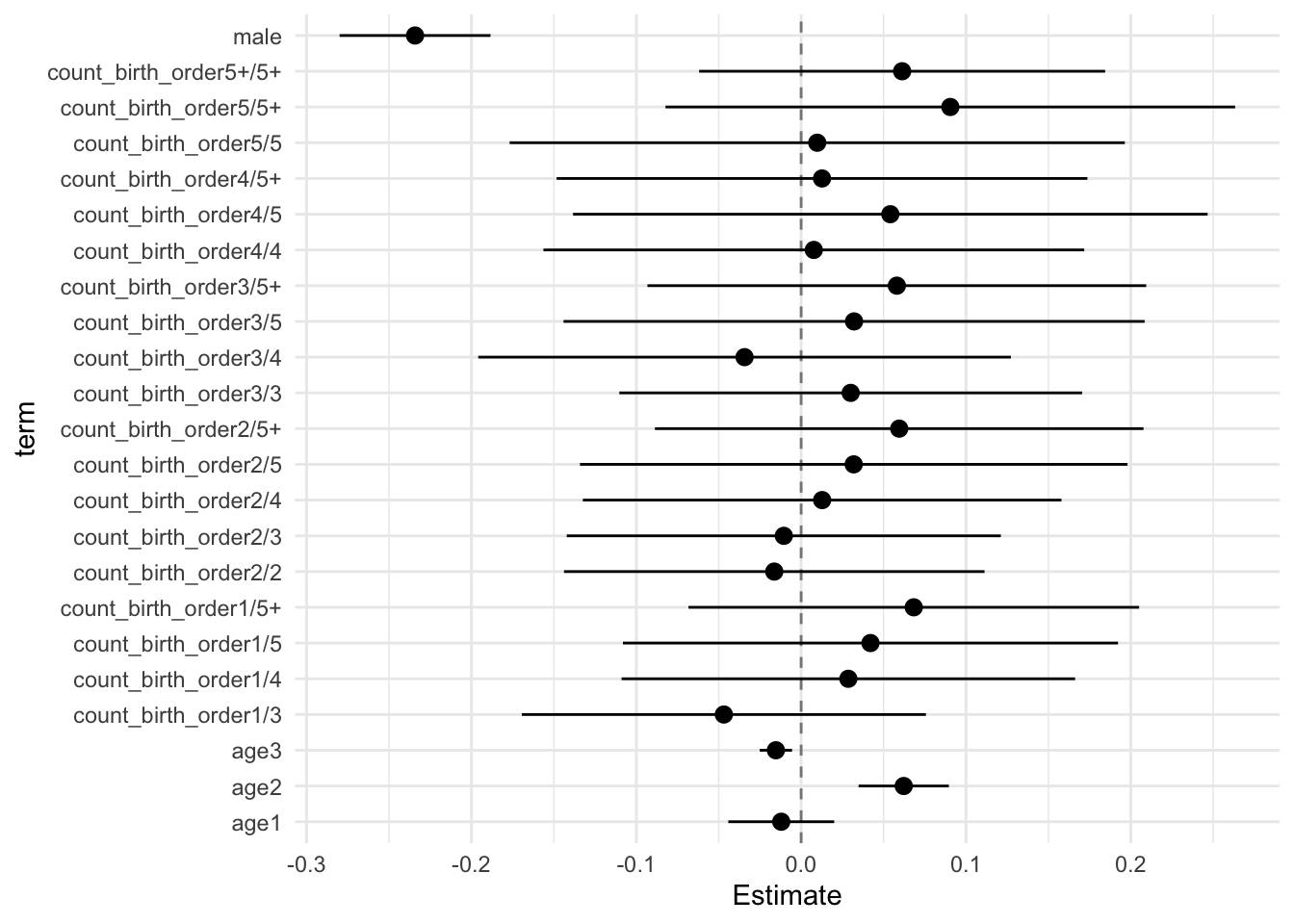
Model Comparison
anova(model_genes_m1, model_genes_m2, model_genes_m3, model_genes_m4)##
## Call:
##
## anova.mitml.result(object = model_genes_m1, model_genes_m2, model_genes_m3,
## model_genes_m4)
##
## Model comparison calculated from 50 imputed data sets.
## Combination method: D3
##
## Model 1: outcome~count_birth_order+poly(age,degree=3,raw=T)+male+(1|mother_pidlink)
## Model 2: outcome~birth_order_nonlinear+poly(age,degree=3,raw=T)+male+sibling_count+(1|mother_pidlink)
## Model 3: outcome~birth_order+poly(age,degree=3,raw=T)+male+sibling_count+(1|mother_pidlink)
## Model 4: outcome~poly(age,degree=3,raw=T)+male+sibling_count+(1|mother_pidlink)
##
## F.value df1 df2 P(>F) RIV
## 1 vs 2: 0.400 10 2818.267 0.947 0.708
## 2 vs 3: 0.034 4 1295.617 0.998 0.621
## 3 vs 4: 0.045 1 212.261 0.832 0.833Risk B
# Specify your outcome
data_used = data_used %>% mutate(outcome = riskB)
data_used_plots <- data_used[[1]]

compare_birthorder_imputed(data_used = data_used)
Parental full sibling order
Basic Model
# with.mitml.list <- function (data, expr, ...)
# {
#     expr <- substitute(expr)
#     parent <- parent.frame()
#     out <- parallel::mclapply(data, function(x) eval(expr, x, parent))
#     class(out) <- c("mitml.result", "list")
#     out
# }
Model Summary
data_used = data_used %>%
  mutate(sibling_count = sibling_count_genes_factor,
         birth_order_nonlinear = birthorder_genes_factor,
         birth_order = birthorder_genes,
         count_birth_order = count_birthorder_genes)

data_used_plots = data_used[[1]]

model_genes_m1 <- with(data_used, lmer(outcome ~ poly(age, degree = 3, raw = T)+ male + sibling_count + (1 | mother_pidlink), REML = FALSE))
x = mitml::testEstimates(model_genes_m1, var.comp = T)

y = as_tibble(x$estimates, rownames = "id")

y = y %>%
  mutate(CI_low = Estimate - 2.576 * Std.Error,
         CI_high = Estimate + 2.576 * Std.Error) %>%
  select(CI_low, CI_high)
CI_low = y$CI_low
CI_high = y$CI_high


x$estimates = cbind(x$estimates[,1:2], CI_low, CI_high, x$estimates[,3:7])
x
##
## Call:
##
## mitml::testEstimates(model = model_genes_m1, var.comp = T)
##
## Final parameter estimates and inferences obtained from 50 imputed data sets.
##
## Estimate Std.Error CI_low CI_high t.value df P(>|t|) RIV FMI
## (Intercept) 0.119 0.028 0.047 0.190 4.282 1015.825 0.000 0.281 0.221
## poly(age, degree = 3, raw = T)1 -0.005 0.012 -0.037 0.026 -0.417 932.594 0.677 0.297 0.231
## poly(age, degree = 3, raw = T)2 0.009 0.011 -0.018 0.036 0.825 1313.703 0.410 0.239 0.194
## poly(age, degree = 3, raw = T)3 -0.004 0.004 -0.014 0.006 -1.096 584.631 0.274 0.407 0.292
## male -0.192 0.017 -0.236 -0.148 -11.258 2078.109 0.000 0.181 0.154
## sibling_count3 -0.031 0.034 -0.120 0.058 -0.902 403.692 0.368 0.535 0.352
## sibling_count4 -0.029 0.035 -0.119 0.061 -0.834 397.974 0.405 0.541 0.354
## sibling_count5 -0.037 0.037 -0.133 0.060 -0.979 372.450 0.328 0.569 0.366
## sibling_count5+ -0.040 0.031 -0.120 0.040 -1.284 622.301 0.199 0.390 0.283
##
## Estimate
## Intercept~~Intercept|mother_pidlink 0.049
## Residual~~Residual 0.941
## ICC|mother_pidlink 0.050
##
## Unadjusted hypothesis test as appropriate in larger samples.x$estimates %>%
as.data.frame() %>%
tibble::rownames_to_column("term") %>%
filter(term != "(Intercept)") %>%
mutate(term = str_replace_all(term, "poly\\(", "")) %>%
mutate(term = str_replace_all(term, ", degree = 3, raw = T\\)", "")) %>%
ggplot(aes(x= term, y = Estimate, ymin = CI_low, ymax = CI_high)) +
geom_hline(yintercept = 0, linetype = "dashed", alpha = 0.5) +
geom_pointrange() +
coord_flip() +
theme_minimal()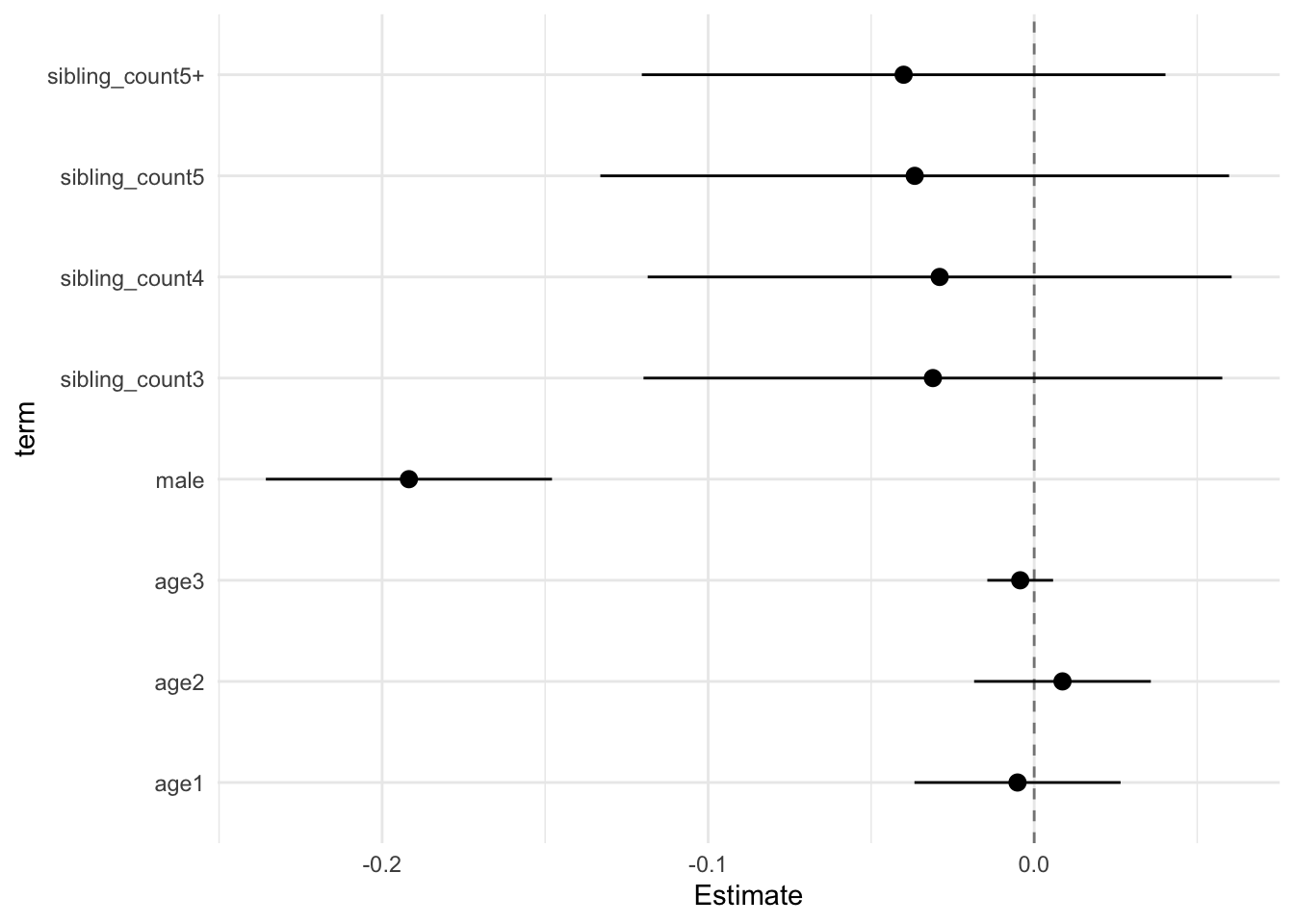
Add Birth Order Linear
Model Summary
model_genes_m2 <- with(data_used, lmer(outcome ~ birth_order + poly(age, degree = 3, raw = T)+ male + sibling_count +
                                         (1 | mother_pidlink), REML = FALSE))
x = mitml::testEstimates(model_genes_m2, var.comp = T)

y = as_tibble(x$estimates, rownames = "id")

y = y %>%
  mutate(CI_low = Estimate - 2.576 * Std.Error,
         CI_high = Estimate + 2.576 * Std.Error) %>%
  select(CI_low, CI_high)
CI_low = y$CI_low
CI_high = y$CI_high


x$estimates = cbind(x$estimates[,1:2], CI_low, CI_high, x$estimates[,3:7])
x
##
## Call:
##
## mitml::testEstimates(model = model_genes_m2, var.comp = T)
##
## Final parameter estimates and inferences obtained from 50 imputed data sets.
##
## Estimate Std.Error CI_low CI_high t.value df P(>|t|) RIV FMI
## (Intercept) 0.114 0.029 0.041 0.188 3.991 1008.539 0.000 0.283 0.222
## birth_order 0.003 0.006 -0.012 0.018 0.559 418.868 0.577 0.520 0.345
## poly(age, degree = 3, raw = T)1 -0.004 0.012 -0.036 0.027 -0.360 853.510 0.719 0.315 0.241
## poly(age, degree = 3, raw = T)2 0.009 0.011 -0.018 0.036 0.842 1306.303 0.400 0.240 0.195
## poly(age, degree = 3, raw = T)3 -0.004 0.004 -0.014 0.006 -1.113 574.883 0.266 0.412 0.294
## male -0.192 0.017 -0.236 -0.148 -11.258 2085.829 0.000 0.181 0.154
## sibling_count3 -0.033 0.034 -0.121 0.056 -0.944 409.661 0.346 0.529 0.349
## sibling_count4 -0.032 0.035 -0.123 0.059 -0.904 378.128 0.367 0.562 0.363
## sibling_count5 -0.041 0.038 -0.140 0.058 -1.071 370.687 0.285 0.571 0.367
## sibling_count5+ -0.048 0.035 -0.138 0.042 -1.379 500.018 0.169 0.456 0.316
##
## Estimate
## Intercept~~Intercept|mother_pidlink 0.049
## Residual~~Residual 0.941
## ICC|mother_pidlink 0.050
##
## Unadjusted hypothesis test as appropriate in larger samples.x$estimates %>%
as.data.frame() %>%
tibble::rownames_to_column("term") %>%
filter(term != "(Intercept)") %>%
mutate(term = str_replace_all(term, "poly\\(", "")) %>%
mutate(term = str_replace_all(term, ", degree = 3, raw = T\\)", "")) %>%
ggplot(aes(x= term, y = Estimate, ymin = CI_low, ymax = CI_high)) +
geom_hline(yintercept = 0, linetype = "dashed", alpha = 0.5) +
geom_pointrange() +
coord_flip() +
theme_minimal()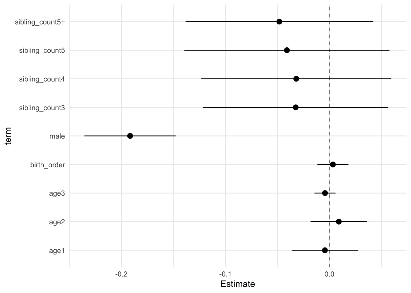
Add Birth Order Factor
Model Summary
model_genes_m3 <- with(data_used, lmer(outcome ~ birth_order_nonlinear + poly(age, degree = 3, raw = T)+ male + sibling_count +
                                         (1 | mother_pidlink), REML = FALSE))
x = mitml::testEstimates(model_genes_m3, var.comp = T)

y = as_tibble(x$estimates, rownames = "id")

y = y %>%
  mutate(CI_low = Estimate - 2.576 * Std.Error,
         CI_high = Estimate + 2.576 * Std.Error) %>%
  select(CI_low, CI_high)
CI_low = y$CI_low
CI_high = y$CI_high


x$estimates = cbind(x$estimates[,1:2], CI_low, CI_high, x$estimates[,3:7])
x
##
## Call:
##
## mitml::testEstimates(model = model_genes_m3, var.comp = T)
##
## Final parameter estimates and inferences obtained from 50 imputed data sets.
##
## Estimate Std.Error CI_low CI_high t.value df P(>|t|) RIV FMI
## (Intercept) 0.108 0.029 0.035 0.182 3.789 1148.860 0.000 0.260 0.208
## birth_order_nonlinear2 0.029 0.028 -0.042 0.100 1.047 231.362 0.296 0.853 0.465
## birth_order_nonlinear3 0.027 0.031 -0.053 0.107 0.854 345.700 0.394 0.604 0.380
## birth_order_nonlinear4 0.021 0.039 -0.079 0.122 0.551 286.726 0.582 0.705 0.417
## birth_order_nonlinear5 0.028 0.052 -0.105 0.161 0.540 248.636 0.589 0.798 0.448
## birth_order_nonlinear5+ 0.032 0.043 -0.078 0.143 0.753 453.059 0.452 0.490 0.332
## poly(age, degree = 3, raw = T)1 -0.004 0.012 -0.036 0.028 -0.354 855.516 0.724 0.315 0.241
## poly(age, degree = 3, raw = T)2 0.009 0.011 -0.018 0.036 0.847 1309.595 0.397 0.240 0.195
## poly(age, degree = 3, raw = T)3 -0.004 0.004 -0.014 0.006 -1.116 573.538 0.265 0.413 0.295
## male -0.192 0.017 -0.236 -0.148 -11.233 1992.699 0.000 0.186 0.158
## sibling_count3 -0.036 0.036 -0.128 0.056 -1.009 356.571 0.314 0.589 0.374
## sibling_count4 -0.036 0.037 -0.130 0.058 -0.979 370.660 0.328 0.571 0.367
## sibling_count5 -0.045 0.040 -0.149 0.059 -1.113 318.505 0.267 0.645 0.396
## sibling_count5+ -0.052 0.035 -0.143 0.039 -1.465 491.005 0.144 0.462 0.319
##
## Estimate
## Intercept~~Intercept|mother_pidlink 0.049
## Residual~~Residual 0.941
## ICC|mother_pidlink 0.050
##
## Unadjusted hypothesis test as appropriate in larger samples.x$estimates %>%
as.data.frame() %>%
tibble::rownames_to_column("term") %>%
filter(term != "(Intercept)") %>%
mutate(term = str_replace_all(term, "poly\\(", "")) %>%
mutate(term = str_replace_all(term, ", degree = 3, raw = T\\)", "")) %>%
ggplot(aes(x= term, y = Estimate, ymin = CI_low, ymax = CI_high)) +
geom_hline(yintercept = 0, linetype = "dashed", alpha = 0.5) +
geom_pointrange() +
coord_flip() +
theme_minimal()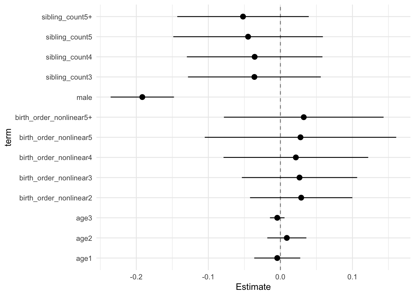
Add Interaction
Model Summary
model_genes_m4 <- with(data_used, lmer(outcome ~ count_birth_order + poly(age, degree = 3, raw = T)+ male  +
                                         (1 | mother_pidlink), REML = FALSE))
x = mitml::testEstimates(model_genes_m4, var.comp = T)

y = as_tibble(x$estimates, rownames = "id")

y = y %>%
  mutate(CI_low = Estimate - 2.576 * Std.Error,
         CI_high = Estimate + 2.576 * Std.Error) %>%
  select(CI_low, CI_high)
CI_low = y$CI_low
CI_high = y$CI_high


x$estimates = cbind(x$estimates[,1:2], CI_low, CI_high, x$estimates[,3:7])
x
##
## Call:
##
## mitml::testEstimates(model = model_genes_m4, var.comp = T)
##
## Final parameter estimates and inferences obtained from 50 imputed data sets.
##
## Estimate Std.Error CI_low CI_high t.value df P(>|t|) RIV FMI
## (Intercept) 0.121 0.034 0.034 0.209 3.569 615.265 0.000 0.393 0.285
## count_birth_order2/2 -0.006 0.056 -0.150 0.138 -0.114 277.398 0.909 0.725 0.424
## count_birth_order1/3 -0.073 0.046 -0.191 0.045 -1.586 403.865 0.113 0.534 0.352
## count_birth_order2/3 -0.000 0.049 -0.126 0.126 -0.001 609.798 1.000 0.396 0.286
## count_birth_order3/3 -0.001 0.055 -0.143 0.141 -0.021 380.084 0.983 0.560 0.362
## count_birth_order1/4 -0.036 0.052 -0.170 0.098 -0.696 283.231 0.487 0.712 0.420
## count_birth_order2/4 -0.020 0.054 -0.158 0.118 -0.366 407.871 0.714 0.530 0.350
## count_birth_order3/4 -0.041 0.058 -0.190 0.108 -0.711 532.855 0.477 0.435 0.306
## count_birth_order4/4 -0.030 0.062 -0.189 0.129 -0.483 277.176 0.630 0.725 0.425
## count_birth_order1/5 -0.045 0.059 -0.197 0.107 -0.756 263.437 0.450 0.758 0.436
## count_birth_order2/5 -0.044 0.068 -0.218 0.131 -0.647 255.301 0.518 0.780 0.442
## count_birth_order3/5 -0.011 0.071 -0.194 0.172 -0.151 312.567 0.880 0.655 0.400
## count_birth_order4/5 -0.045 0.078 -0.245 0.155 -0.577 297.811 0.564 0.682 0.410
## count_birth_order5/5 -0.047 0.075 -0.240 0.146 -0.626 244.211 0.532 0.811 0.452
## count_birth_order1/5+ -0.071 0.051 -0.203 0.061 -1.385 323.558 0.167 0.637 0.393
## count_birth_order2/5+ -0.025 0.055 -0.168 0.117 -0.455 352.984 0.649 0.594 0.376
## count_birth_order3/5+ -0.058 0.064 -0.222 0.106 -0.908 251.199 0.365 0.791 0.446
## count_birth_order4/5+ -0.034 0.063 -0.195 0.127 -0.543 401.682 0.587 0.537 0.352
## count_birth_order5/5+ -0.020 0.065 -0.187 0.146 -0.314 564.729 0.753 0.418 0.297
## count_birth_order5+/5+ -0.032 0.046 -0.150 0.087 -0.692 597.617 0.489 0.401 0.289
## poly(age, degree = 3, raw = T)1 -0.005 0.012 -0.037 0.027 -0.367 826.216 0.714 0.322 0.245
## poly(age, degree = 3, raw = T)2 0.009 0.011 -0.019 0.036 0.821 1261.785 0.412 0.245 0.198
## poly(age, degree = 3, raw = T)3 -0.004 0.004 -0.014 0.006 -1.093 558.490 0.275 0.421 0.299
## male -0.192 0.017 -0.236 -0.148 -11.231 1974.525 0.000 0.187 0.158
##
## Estimate
## Intercept~~Intercept|mother_pidlink 0.049
## Residual~~Residual 0.940
## ICC|mother_pidlink 0.050
##
## Unadjusted hypothesis test as appropriate in larger samples.x$estimates %>%
as.data.frame() %>%
tibble::rownames_to_column("term") %>%
filter(term != "(Intercept)") %>%
mutate(term = str_replace_all(term, "poly\\(", "")) %>%
mutate(term = str_replace_all(term, ", degree = 3, raw = T\\)", "")) %>%
ggplot(aes(x= term, y = Estimate, ymin = CI_low, ymax = CI_high)) +
geom_hline(yintercept = 0, linetype = "dashed", alpha = 0.5) +
geom_pointrange() +
coord_flip() +
theme_minimal()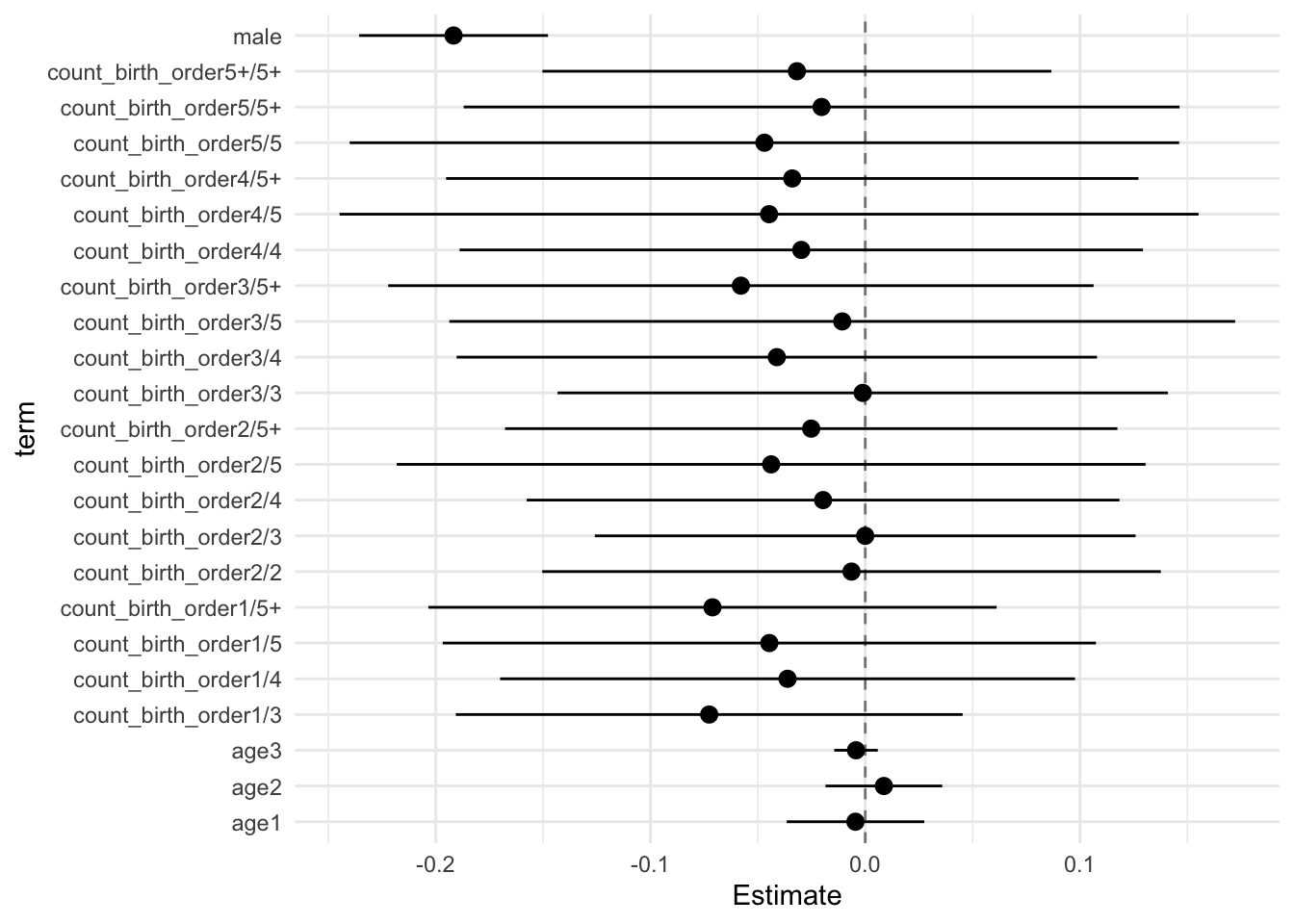
Model Comparison
anova(model_genes_m1, model_genes_m2, model_genes_m3, model_genes_m4)##
## Call:
##
## anova.mitml.result(object = model_genes_m1, model_genes_m2, model_genes_m3,
## model_genes_m4)
##
## Model comparison calculated from 50 imputed data sets.
## Combination method: D3
##
## Model 1: outcome~count_birth_order+poly(age,degree=3,raw=T)+male+(1|mother_pidlink)
## Model 2: outcome~birth_order_nonlinear+poly(age,degree=3,raw=T)+male+sibling_count+(1|mother_pidlink)
## Model 3: outcome~birth_order+poly(age,degree=3,raw=T)+male+sibling_count+(1|mother_pidlink)
## Model 4: outcome~poly(age,degree=3,raw=T)+male+sibling_count+(1|mother_pidlink)
##
## F.value df1 df2 P(>F) RIV
## 1 vs 2: 0.222 10 2816.721 0.994 0.708
## 2 vs 3: 0.327 4 1067.811 0.860 0.731
## 3 vs 4: 0.316 1 371.534 0.574 0.516Educational Attainment
Years of Education - z-standardized
# Specify your outcome
data_used = data_used %>% mutate(outcome = years_of_education_z)
data_used_plots <- data_used[[1]]

compare_birthorder_imputed(data_used = data_used)
Parental full sibling order
Basic Model
# with.mitml.list <- function (data, expr, ...)
# {
#     expr <- substitute(expr)
#     parent <- parent.frame()
#     out <- parallel::mclapply(data, function(x) eval(expr, x, parent))
#     class(out) <- c("mitml.result", "list")
#     out
# }
Model Summary
data_used = data_used %>%
  mutate(sibling_count = sibling_count_genes_factor,
         birth_order_nonlinear = birthorder_genes_factor,
         birth_order = birthorder_genes,
         count_birth_order = count_birthorder_genes)

data_used_plots = data_used[[1]]

model_genes_m1 <- with(data_used, lmer(outcome ~ poly(age, degree = 3, raw = T)+ male + sibling_count + (1 | mother_pidlink), REML = FALSE))
x = mitml::testEstimates(model_genes_m1, var.comp = T)

y = as_tibble(x$estimates, rownames = "id")

y = y %>%
  mutate(CI_low = Estimate - 2.576 * Std.Error,
         CI_high = Estimate + 2.576 * Std.Error) %>%
  select(CI_low, CI_high)
CI_low = y$CI_low
CI_high = y$CI_high


x$estimates = cbind(x$estimates[,1:2], CI_low, CI_high, x$estimates[,3:7])
x
##
## Call:
##
## mitml::testEstimates(model = model_genes_m1, var.comp = T)
##
## Final parameter estimates and inferences obtained from 50 imputed data sets.
##
## Estimate Std.Error CI_low CI_high t.value df P(>|t|) RIV FMI
## (Intercept) 0.308 0.029 0.233 0.382 10.634 1044.951 0.000 0.276 0.218
## poly(age, degree = 3, raw = T)1 -0.072 0.011 -0.101 -0.044 -6.605 4777.536 0.000 0.113 0.102
## poly(age, degree = 3, raw = T)2 -0.222 0.009 -0.245 -0.199 -25.386 6039.764 0.000 0.099 0.090
## poly(age, degree = 3, raw = T)3 0.044 0.003 0.036 0.052 14.275 9771.468 0.000 0.076 0.071
## male -0.025 0.014 -0.060 0.011 -1.778 2002.401 0.076 0.185 0.157
## sibling_count3 0.024 0.036 -0.068 0.117 0.675 830.114 0.500 0.321 0.245
## sibling_count4 -0.070 0.039 -0.169 0.030 -1.806 533.800 0.071 0.435 0.306
## sibling_count5 -0.165 0.046 -0.282 -0.047 -3.617 288.304 0.000 0.701 0.416
## sibling_count5+ -0.251 0.038 -0.348 -0.154 -6.649 451.012 0.000 0.492 0.333
##
## Estimate
## Intercept~~Intercept|mother_pidlink 0.487
## Residual~~Residual 0.449
## ICC|mother_pidlink 0.520
##
## Unadjusted hypothesis test as appropriate in larger samples.x$estimates %>%
as.data.frame() %>%
tibble::rownames_to_column("term") %>%
filter(term != "(Intercept)") %>%
mutate(term = str_replace_all(term, "poly\\(", "")) %>%
mutate(term = str_replace_all(term, ", degree = 3, raw = T\\)", "")) %>%
ggplot(aes(x= term, y = Estimate, ymin = CI_low, ymax = CI_high)) +
geom_hline(yintercept = 0, linetype = "dashed", alpha = 0.5) +
geom_pointrange() +
coord_flip() +
theme_minimal()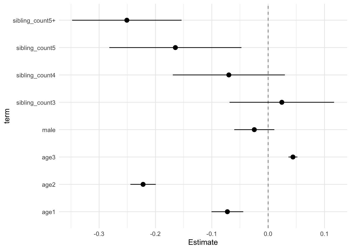
Add Birth Order Linear
Model Summary
model_genes_m2 <- with(data_used, lmer(outcome ~ birth_order + poly(age, degree = 3, raw = T)+ male + sibling_count +
                                         (1 | mother_pidlink), REML = FALSE))
x = mitml::testEstimates(model_genes_m2, var.comp = T)

y = as_tibble(x$estimates, rownames = "id")

y = y %>%
  mutate(CI_low = Estimate - 2.576 * Std.Error,
         CI_high = Estimate + 2.576 * Std.Error) %>%
  select(CI_low, CI_high)
CI_low = y$CI_low
CI_high = y$CI_high


x$estimates = cbind(x$estimates[,1:2], CI_low, CI_high, x$estimates[,3:7])
x
##
## Call:
##
## mitml::testEstimates(model = model_genes_m2, var.comp = T)
##
## Final parameter estimates and inferences obtained from 50 imputed data sets.
##
## Estimate Std.Error CI_low CI_high t.value df P(>|t|) RIV FMI
## (Intercept) 0.312 0.030 0.236 0.388 10.548 942.442 0.000 0.295 0.230
## birth_order -0.004 0.005 -0.017 0.009 -0.790 320.857 0.430 0.641 0.395
## poly(age, degree = 3, raw = T)1 -0.074 0.011 -0.103 -0.045 -6.618 3652.547 0.000 0.131 0.116
## poly(age, degree = 3, raw = T)2 -0.222 0.009 -0.244 -0.199 -25.388 6073.444 0.000 0.099 0.090
## poly(age, degree = 3, raw = T)3 0.044 0.003 0.036 0.052 14.294 9534.136 0.000 0.077 0.072
## male -0.025 0.014 -0.060 0.011 -1.781 2018.682 0.075 0.185 0.157
## sibling_count3 0.026 0.036 -0.067 0.120 0.728 807.536 0.467 0.327 0.248
## sibling_count4 -0.065 0.039 -0.165 0.034 -1.687 551.357 0.092 0.425 0.301
## sibling_count5 -0.159 0.046 -0.276 -0.041 -3.477 309.111 0.001 0.662 0.402
## sibling_count5+ -0.240 0.041 -0.345 -0.135 -5.906 389.106 0.000 0.550 0.358
##
## Estimate
## Intercept~~Intercept|mother_pidlink 0.488
## Residual~~Residual 0.449
## ICC|mother_pidlink 0.521
##
## Unadjusted hypothesis test as appropriate in larger samples.x$estimates %>%
as.data.frame() %>%
tibble::rownames_to_column("term") %>%
filter(term != "(Intercept)") %>%
mutate(term = str_replace_all(term, "poly\\(", "")) %>%
mutate(term = str_replace_all(term, ", degree = 3, raw = T\\)", "")) %>%
ggplot(aes(x= term, y = Estimate, ymin = CI_low, ymax = CI_high)) +
geom_hline(yintercept = 0, linetype = "dashed", alpha = 0.5) +
geom_pointrange() +
coord_flip() +
theme_minimal()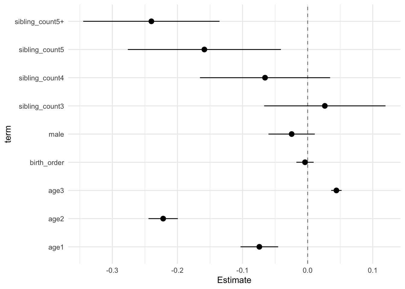
Add Birth Order Factor
Model Summary
model_genes_m3 <- with(data_used, lmer(outcome ~ birth_order_nonlinear + poly(age, degree = 3, raw = T)+ male + sibling_count +
                                         (1 | mother_pidlink), REML = FALSE))
x = mitml::testEstimates(model_genes_m3, var.comp = T)

y = as_tibble(x$estimates, rownames = "id")

y = y %>%
  mutate(CI_low = Estimate - 2.576 * Std.Error,
         CI_high = Estimate + 2.576 * Std.Error) %>%
  select(CI_low, CI_high)
CI_low = y$CI_low
CI_high = y$CI_high


x$estimates = cbind(x$estimates[,1:2], CI_low, CI_high, x$estimates[,3:7])
x
##
## Call:
##
## mitml::testEstimates(model = model_genes_m3, var.comp = T)
##
## Final parameter estimates and inferences obtained from 50 imputed data sets.
##
## Estimate Std.Error CI_low CI_high t.value df P(>|t|) RIV FMI
## (Intercept) 0.321 0.029 0.247 0.395 11.124 1439.564 0.000 0.226 0.186
## birth_order_nonlinear2 -0.044 0.022 -0.099 0.012 -2.016 245.671 0.045 0.807 0.451
## birth_order_nonlinear3 -0.013 0.027 -0.082 0.056 -0.480 224.707 0.632 0.876 0.472
## birth_order_nonlinear4 -0.002 0.031 -0.083 0.078 -0.072 277.885 0.942 0.724 0.424
## birth_order_nonlinear5 0.005 0.040 -0.097 0.108 0.133 293.327 0.895 0.691 0.413
## birth_order_nonlinear5+ -0.043 0.037 -0.140 0.054 -1.148 321.208 0.252 0.641 0.394
## poly(age, degree = 3, raw = T)1 -0.073 0.011 -0.102 -0.044 -6.545 3660.856 0.000 0.131 0.116
## poly(age, degree = 3, raw = T)2 -0.221 0.009 -0.244 -0.199 -25.328 6349.465 0.000 0.096 0.088
## poly(age, degree = 3, raw = T)3 0.044 0.003 0.036 0.052 14.250 10282.804 0.000 0.074 0.069
## male -0.025 0.014 -0.060 0.011 -1.786 2070.051 0.074 0.182 0.155
## sibling_count3 0.026 0.036 -0.068 0.120 0.704 804.804 0.482 0.328 0.249
## sibling_count4 -0.070 0.039 -0.171 0.032 -1.769 537.605 0.077 0.432 0.304
## sibling_count5 -0.168 0.046 -0.287 -0.048 -3.610 301.304 0.000 0.676 0.407
## sibling_count5+ -0.244 0.041 -0.349 -0.139 -5.995 392.543 0.000 0.546 0.357
##
## Estimate
## Intercept~~Intercept|mother_pidlink 0.488
## Residual~~Residual 0.448
## ICC|mother_pidlink 0.521
##
## Unadjusted hypothesis test as appropriate in larger samples.x$estimates %>%
as.data.frame() %>%
tibble::rownames_to_column("term") %>%
filter(term != "(Intercept)") %>%
mutate(term = str_replace_all(term, "poly\\(", "")) %>%
mutate(term = str_replace_all(term, ", degree = 3, raw = T\\)", "")) %>%
ggplot(aes(x= term, y = Estimate, ymin = CI_low, ymax = CI_high)) +
geom_hline(yintercept = 0, linetype = "dashed", alpha = 0.5) +
geom_pointrange() +
coord_flip() +
theme_minimal()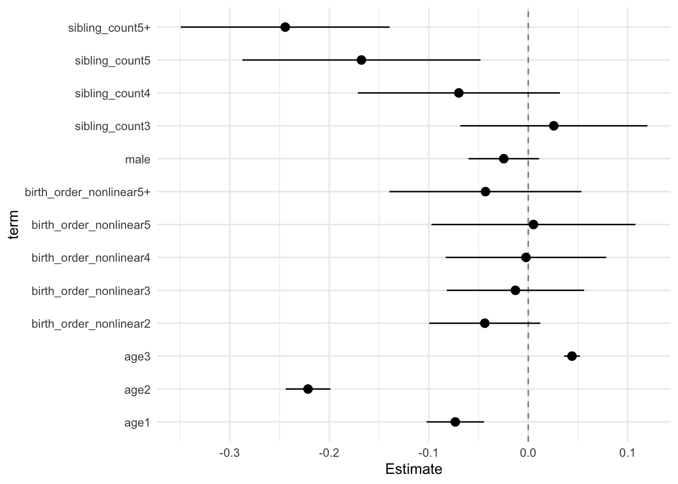
Add Interaction
Model Summary
model_genes_m4 <- with(data_used, lmer(outcome ~ count_birth_order + poly(age, degree = 3, raw = T)+ male  +
                                         (1 | mother_pidlink), REML = FALSE))
x = mitml::testEstimates(model_genes_m4, var.comp = T)

y = as_tibble(x$estimates, rownames = "id")

y = y %>%
  mutate(CI_low = Estimate - 2.576 * Std.Error,
         CI_high = Estimate + 2.576 * Std.Error) %>%
  select(CI_low, CI_high)
CI_low = y$CI_low
CI_high = y$CI_high


x$estimates = cbind(x$estimates[,1:2], CI_low, CI_high, x$estimates[,3:7])
x
##
## Call:
##
## mitml::testEstimates(model = model_genes_m4, var.comp = T)
##
## Final parameter estimates and inferences obtained from 50 imputed data sets.
##
## Estimate Std.Error CI_low CI_high t.value df P(>|t|) RIV FMI
## (Intercept) 0.327 0.031 0.249 0.406 10.709 1685.533 0.000 0.206 0.171
## count_birth_order2/2 -0.067 0.040 -0.170 0.035 -1.699 771.028 0.090 0.337 0.254
## count_birth_order1/3 0.041 0.043 -0.071 0.153 0.943 564.088 0.346 0.418 0.297
## count_birth_order2/3 -0.040 0.046 -0.158 0.079 -0.869 717.048 0.385 0.354 0.263
## count_birth_order3/3 -0.023 0.049 -0.149 0.103 -0.476 626.651 0.634 0.388 0.282
## count_birth_order1/4 -0.084 0.046 -0.203 0.036 -1.799 573.781 0.073 0.413 0.295
## count_birth_order2/4 -0.118 0.049 -0.245 0.008 -2.417 582.054 0.016 0.409 0.293
## count_birth_order3/4 -0.068 0.053 -0.204 0.068 -1.291 608.932 0.197 0.396 0.286
## count_birth_order4/4 -0.091 0.051 -0.222 0.041 -1.782 687.214 0.075 0.364 0.269
## count_birth_order1/5 -0.188 0.060 -0.343 -0.033 -3.120 219.303 0.002 0.896 0.477
## count_birth_order2/5 -0.205 0.063 -0.368 -0.043 -3.252 265.077 0.001 0.754 0.434
## count_birth_order3/5 -0.172 0.063 -0.335 -0.010 -2.727 371.330 0.007 0.571 0.367
## count_birth_order4/5 -0.174 0.068 -0.349 0.001 -2.560 347.088 0.011 0.602 0.379
## count_birth_order5/5 -0.180 0.066 -0.349 -0.010 -2.728 298.500 0.007 0.681 0.409
## count_birth_order1/5+ -0.278 0.049 -0.405 -0.151 -5.633 356.470 0.000 0.589 0.374
## count_birth_order2/5+ -0.275 0.052 -0.409 -0.142 -5.316 369.303 0.000 0.573 0.368
## count_birth_order3/5+ -0.263 0.060 -0.418 -0.108 -4.366 217.895 0.000 0.902 0.479
## count_birth_order4/5+ -0.240 0.057 -0.387 -0.093 -4.216 370.779 0.000 0.571 0.367
## count_birth_order5/5+ -0.235 0.058 -0.385 -0.085 -4.045 483.106 0.000 0.467 0.321
## count_birth_order5+/5+ -0.293 0.046 -0.412 -0.174 -6.361 513.564 0.000 0.447 0.312
## poly(age, degree = 3, raw = T)1 -0.074 0.011 -0.103 -0.045 -6.572 3443.492 0.000 0.135 0.120
## poly(age, degree = 3, raw = T)2 -0.221 0.009 -0.243 -0.198 -25.135 5733.846 0.000 0.102 0.093
## poly(age, degree = 3, raw = T)3 0.044 0.003 0.036 0.052 14.170 9200.721 0.000 0.079 0.073
## male -0.024 0.014 -0.060 0.011 -1.764 2132.213 0.078 0.179 0.152
##
## Estimate
## Intercept~~Intercept|mother_pidlink 0.488
## Residual~~Residual 0.448
## ICC|mother_pidlink 0.522
##
## Unadjusted hypothesis test as appropriate in larger samples.x$estimates %>%
as.data.frame() %>%
tibble::rownames_to_column("term") %>%
filter(term != "(Intercept)") %>%
mutate(term = str_replace_all(term, "poly\\(", "")) %>%
mutate(term = str_replace_all(term, ", degree = 3, raw = T\\)", "")) %>%
ggplot(aes(x= term, y = Estimate, ymin = CI_low, ymax = CI_high)) +
geom_hline(yintercept = 0, linetype = "dashed", alpha = 0.5) +
geom_pointrange() +
coord_flip() +
theme_minimal()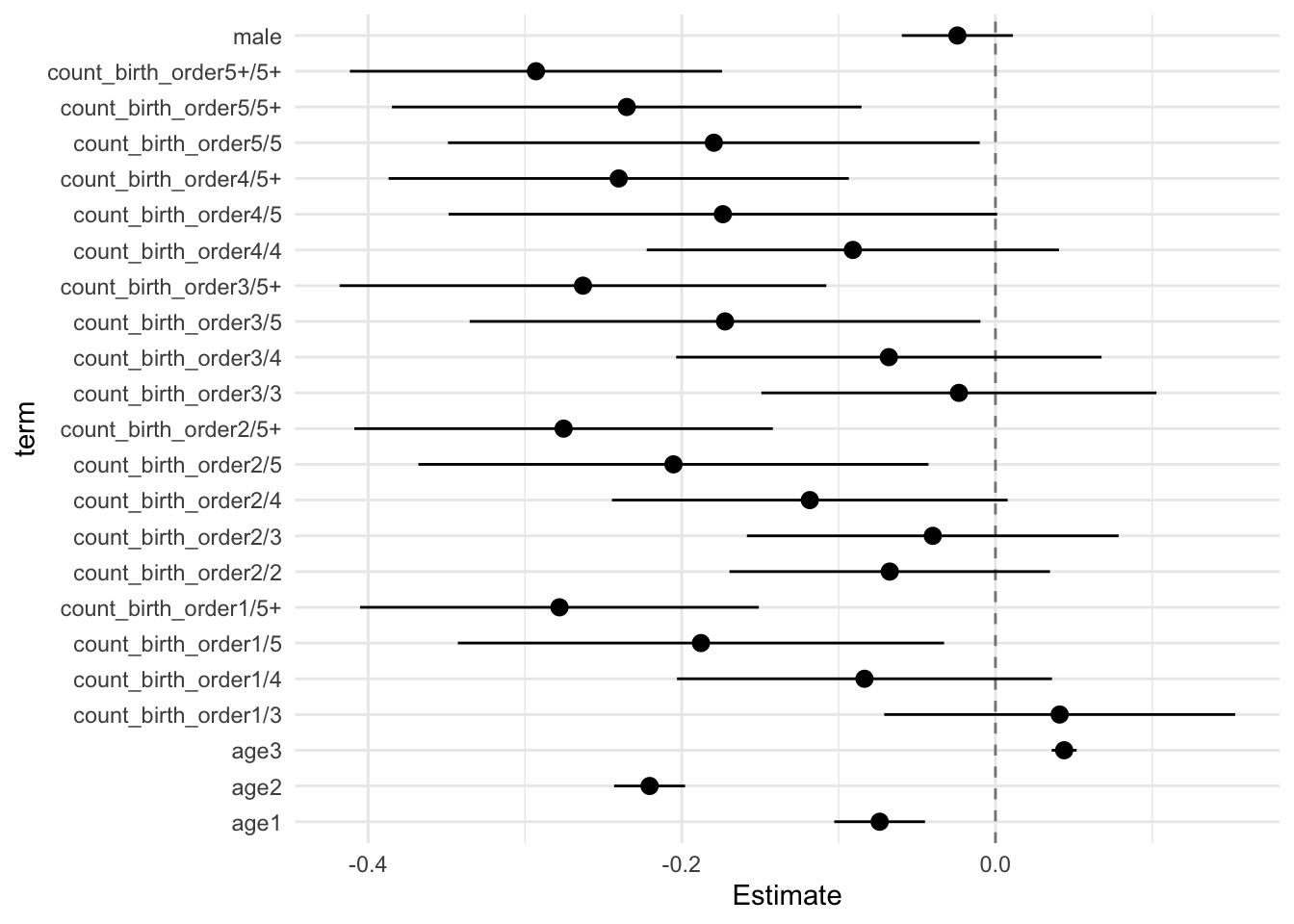
Model Comparison
anova(model_genes_m1, model_genes_m2, model_genes_m3, model_genes_m4)##
## Call:
##
## anova.mitml.result(object = model_genes_m1, model_genes_m2, model_genes_m3,
## model_genes_m4)
##
## Model comparison calculated from 50 imputed data sets.
## Combination method: D3
##
## Model 1: outcome~count_birth_order+poly(age,degree=3,raw=T)+male+(1|mother_pidlink)
## Model 2: outcome~birth_order_nonlinear+poly(age,degree=3,raw=T)+male+sibling_count+(1|mother_pidlink)
## Model 3: outcome~birth_order+poly(age,degree=3,raw=T)+male+sibling_count+(1|mother_pidlink)
## Model 4: outcome~poly(age,degree=3,raw=T)+male+sibling_count+(1|mother_pidlink)
##
## F.value df1 df2 P(>F) RIV
## 1 vs 2: 0.363 10 2740.231 0.962 0.725
## 2 vs 3: 1.240 4 1006.440 0.292 0.770
## 3 vs 4: 0.625 1 283.201 0.430 0.643LS0tCnRpdGxlOiAiNC4gQW5hbHlzZXMgSW1wdXRlZCBEYXRhIgphdXRob3I6ICJMYXVyYSBCb3R6ZXQgJiBSdWJlbiBBcnNsYW4iCm91dHB1dDogaHRtbF9kb2N1bWVudAplZGl0b3Jfb3B0aW9uczogCiAgY2h1bmtfb3V0cHV0X3R5cGU6IGNvbnNvbGUKLS0tCgojIDxzcGFuIHN0eWxlPSJjb2xvcjojRkZEOTJGIj5CaXJ0aCBPcmRlciBFZmZlY3RzIEltcHV0ZWQgRGF0YTwvc3Bhbj4gey50YWJzZXR9CgojIyBIZWxwZXIKCmBgYHtyIGhlbHBlcn0Kc291cmNlKCIwX2hlbHBlcnMuUiIpCm9wdHNfY2h1bmskc2V0KHdhcm5pbmcgPSBGQUxTRSwgZXJyb3IgPSBUKQpkZXRhY2goInBhY2thZ2U6bG1lclRlc3QiLCB1bmxvYWQgPSBUUlVFKQpgYGAKCgojIyBGdW5jdGlvbnMKCmBgYHtyfQpvcHRpb25zKG1jLmNvcmVzPTQpCm5faW1wdXRhdGlvbnMubWl0bWwgPSBmdW5jdGlvbihpbXBzKSB7CiAgaW1wcyRpdGVyJG0KfQpuX2ltcHV0YXRpb25zLm1pZHMgPSBmdW5jdGlvbihpbXBzKSB7CiAgaW1wcyRtCn0Kbl9pbXB1dGF0aW9ucy5hbWVsaWEgPSBmdW5jdGlvbihpbXBzKSB7CiAgbGVuZ3RoKGltcHMkaW1wdXRhdGlvbnMpCn0Kbl9pbXB1dGF0aW9ucyA9IGZ1bmN0aW9uKGltcHMpIHsgVXNlTWV0aG9kKCJuX2ltcHV0YXRpb25zIikgfQoKY29tcGxldGUubWl0bWwgPSBtaXRtbDo6bWl0bWxDb21wbGV0ZQpjb21wbGV0ZS5taWRzID0gbWljZTo6Y29tcGxldGUKY29tcGxldGUgPSBmdW5jdGlvbiguLi4pIHsgVXNlTWV0aG9kKCJjb21wbGV0ZSIpIH0KCmxpYnJhcnkobWljZSkKbGlicmFyeShtaWNlYWRkcykKbGlicmFyeShtaXRtbCkKYGBgCgoKIyMgTG9hZCBkYXRhCgpgYGB7ciBMb2FkIERhdGF9CmJpcnRob3JkZXJfbWlzc2luZyA9IHJlYWRSRFMoImRhdGEvYWxsZGF0YV9iaXJ0aG9yZGVyX21pc3NpbmcucmRzIikKYmlydGhvcmRlciA9IHJlYWRSRFMoImRhdGEvYWxsZGF0YV9iaXJ0aG9yZGVyX2lfbWw1LnJkcyIpCmBgYAoKIyMgRGF0YSBwcmVwYXJhdGlvbnMKCmBgYHtyIGRhdGEgcHJlcGFyYXRpb25zfQpiaXJ0aG9yZGVyIDwtIG1pZHMybWl0bWwubGlzdChiaXJ0aG9yZGVyKQoKIyMgQ2FsY3VsYXRlIGdfZmFjdG9ycyAoZm9yIG5vdyB3aXRoIHJvd01lYW5zOiBiZXR0ZXIgdG8gcnVuIGZhY3RvciBhbmFseXNpcyBoZXJlIGFzIHdlbGw/KQpiaXJ0aG9yZGVyIDwtIHdpdGhpbihiaXJ0aG9yZGVyLCB7CiAgZ19mYWN0b3JfMjAxNV9vbGQgPC0gcm93TWVhbnMoc2NhbGUoY2JpbmQocmF2ZW5fMjAxNV9vbGQsIG1hdGhfMjAxNV9vbGQsIGNvdW50X2JhY2t3YXJkcywgIHdvcmRzX2RlbGF5ZWQsIGFkYXB0aXZlX251bWJlcmluZykpKQp9KQoKYmlydGhvcmRlciA8LSB3aXRoaW4oYmlydGhvcmRlciwgewogIGdfZmFjdG9yXzIwMTVfeW91bmcgPC0gcm93TWVhbnMoc2NhbGUoY2JpbmQocmF2ZW5fMjAxNV95b3VuZywgbWF0aF8yMDE1X3lvdW5nKSkpCn0pCgpiaXJ0aG9yZGVyIDwtIHdpdGhpbihiaXJ0aG9yZGVyLCB7CiAgZ19mYWN0b3JfMjAwN19vbGQgPC0gcm93TWVhbnMoc2NhbGUoY2JpbmQocmF2ZW5fMjAwN19vbGQsIG1hdGhfMjAwN19vbGQpKSkKfSkKCmJpcnRob3JkZXIgPC0gd2l0aGluKGJpcnRob3JkZXIsIHsKICBnX2ZhY3Rvcl8yMDA3X3lvdW5nIDwtIHJvd01lYW5zKHNjYWxlKGNiaW5kKHJhdmVuXzIwMDdfeW91bmcsIG1hdGhfMjAwN195b3VuZykpKQp9KQoKCmJpcnRob3JkZXIgPSBiaXJ0aG9yZGVyICU+JSB0YmxfZGYubWl0bWwubGlzdAoKIyMjIEJpcnRob3JkZXIgYW5kIFNpYmxpbmcgQ291bnQKYmlydGhvcmRlcl9kYXRhID0gYmlydGhvcmRlcltbMV1dCgpiaXJ0aG9yZGVyID0gYmlydGhvcmRlciAlPiUKICBtdXRhdGUoYmlydGhvcmRlcl9nZW5lcyA9IGlmZWxzZShiaXJ0aG9yZGVyX2dlbmVzIDwgMSwgMSwgYmlydGhvcmRlcl9nZW5lcyksCiAgICAgICAgIGJpcnRob3JkZXJfbmFpdmUgPSBpZmVsc2UoYmlydGhvcmRlcl9uYWl2ZSA8IDEsIDEsIGJpcnRob3JkZXJfbmFpdmUpLAogICAgICAgICBiaXJ0aG9yZGVyX2dlbmVzID0gcm91bmQoYmlydGhvcmRlcl9nZW5lcyksCiAgICAgICAgIGJpcnRob3JkZXJfbmFpdmUgPSByb3VuZChiaXJ0aG9yZGVyX25haXZlKSwKICAgICAgICAgc2libGluZ19jb3VudF9nZW5lcyA9IGlmZWxzZShzaWJsaW5nX2NvdW50X2dlbmVzIDwgMiwgMiwgc2libGluZ19jb3VudF9nZW5lcyksCiAgICAgICAgIHNpYmxpbmdfY291bnRfbmFpdmUgPSBpZmVsc2Uoc2libGluZ19jb3VudF9uYWl2ZSA8IDIsIDIsIHNpYmxpbmdfY291bnRfbmFpdmUpLAogICAgICAgICBzaWJsaW5nX2NvdW50X2dlbmVzID0gcm91bmQoc2libGluZ19jb3VudF9nZW5lcyksCiAgICAgICAgIHNpYmxpbmdfY291bnRfbmFpdmUgPSByb3VuZChzaWJsaW5nX2NvdW50X25haXZlKQogICAgICAgICApICU+JSAKICBncm91cF9ieShtb3RoZXJfcGlkbGluaykgJT4lIAogICMgbWFrZSBzdXJlIHNpYmxpbmcgY291bnQgaXMgY29uc2lzdGVudCB3aXRoIGJpcnRoIG9yZGVyIChmb3Igd2hpY2ggaW1wdXRhdGlvbiBtb2RlbCBzZWVtcyB0byB3b3JrIGJldHRlcikKICBtdXRhdGUoc2libGluZ19jb3VudF9nZW5lcyA9IG1heChiaXJ0aG9yZGVyX2dlbmVzLCBzaWJsaW5nX2NvdW50X2dlbmVzKSkgJT4lIAogIHVuZ3JvdXAoKQoKCmJpcnRob3JkZXIgPSBiaXJ0aG9yZGVyICU+JSAKICBtdXRhdGUoCiMgYmlydGhvcmRlciBhcyBmYWN0b3JzIHdpdGggbGV2ZWxzIG9mIDEsIDIsIDMsIDQsIDUsIDUrCiAgICBiaXJ0aG9yZGVyX25haXZlX2ZhY3RvciA9IGFzLmNoYXJhY3RlcihiaXJ0aG9yZGVyX25haXZlKSwKICAgIGJpcnRob3JkZXJfbmFpdmVfZmFjdG9yID0gaWZlbHNlKGJpcnRob3JkZXJfbmFpdmUgPiA1LCAiNSsiLAogICAgICAgICAgICAgICAgICAgICAgICAgICAgICAgICAgICAgICAgICAgIGJpcnRob3JkZXJfbmFpdmVfZmFjdG9yKSwKICAgIGJpcnRob3JkZXJfbmFpdmVfZmFjdG9yID0gZmFjdG9yKGJpcnRob3JkZXJfbmFpdmVfZmFjdG9yLCAKICAgICAgICAgICAgICAgICAgICAgICAgICAgICAgICAgICAgICAgICAgICBsZXZlbHMgPSBjKCIxIiwiMiIsIjMiLCI0IiwiNSIsIjUrIikpLAogICAgc2libGluZ19jb3VudF9uYWl2ZV9mYWN0b3IgPSBhcy5jaGFyYWN0ZXIoc2libGluZ19jb3VudF9uYWl2ZSksCiAgICBzaWJsaW5nX2NvdW50X25haXZlX2ZhY3RvciA9IGlmZWxzZShzaWJsaW5nX2NvdW50X25haXZlID4gNSwgIjUrIiwKICAgICAgICAgICAgICAgICAgICAgICAgICAgICAgICAgICAgICAgICAgICAgICBzaWJsaW5nX2NvdW50X25haXZlX2ZhY3RvciksCiAgICBzaWJsaW5nX2NvdW50X25haXZlX2ZhY3RvciA9IGZhY3RvcihzaWJsaW5nX2NvdW50X25haXZlX2ZhY3RvciwgCiAgICAgICAgICAgICAgICAgICAgICAgICAgICAgICAgICAgICAgICAgICAgICAgbGV2ZWxzID0gYygiMiIsIjMiLCI0IiwiNSIsIjUrIikpLAogICAgYmlydGhvcmRlcl9nZW5lc19mYWN0b3IgPSBhcy5jaGFyYWN0ZXIoYmlydGhvcmRlcl9nZW5lcyksCiAgICBiaXJ0aG9yZGVyX2dlbmVzX2ZhY3RvciA9IGlmZWxzZShiaXJ0aG9yZGVyX2dlbmVzID41ICwgIjUrIiwgYmlydGhvcmRlcl9nZW5lc19mYWN0b3IpLAogICAgYmlydGhvcmRlcl9nZW5lc19mYWN0b3IgPSBmYWN0b3IoYmlydGhvcmRlcl9nZW5lc19mYWN0b3IsIAogICAgICAgICAgICAgICAgICAgICAgICAgICAgICAgICAgICAgbGV2ZWxzID0gYygiMSIsIjIiLCIzIiwiNCIsIjUiLCI1KyIpKSwKICAgIHNpYmxpbmdfY291bnRfZ2VuZXNfZmFjdG9yID0gYXMuY2hhcmFjdGVyKHNpYmxpbmdfY291bnRfZ2VuZXMpLAogICAgc2libGluZ19jb3VudF9nZW5lc19mYWN0b3IgPSBpZmVsc2Uoc2libGluZ19jb3VudF9nZW5lcyA+NSAsICI1KyIsCiAgICAgICAgICAgICAgICAgICAgICAgICAgICAgICAgICAgICAgICBzaWJsaW5nX2NvdW50X2dlbmVzX2ZhY3RvciksCiAgICBzaWJsaW5nX2NvdW50X2dlbmVzX2ZhY3RvciA9IGZhY3RvcihzaWJsaW5nX2NvdW50X2dlbmVzX2ZhY3RvciwgCiAgICAgICAgICAgICAgICAgICAgICAgICAgICAgICAgICAgICAgICBsZXZlbHMgPSBjKCIyIiwiMyIsIjQiLCI1IiwiNSsiKSksCiAgICAjIGludGVyYWN0aW9uIGJpcnRob3JkZXIgKiBzaWJsaW5nY291dCBmb3IgZWFjaCBiaXJ0aG9yZGVyCiAgICBjb3VudF9iaXJ0aG9yZGVyX25haXZlID0KICAgICAgZmFjdG9yKHN0cl9yZXBsYWNlKGFzLmNoYXJhY3RlcihpbnRlcmFjdGlvbihiaXJ0aG9yZGVyX25haXZlX2ZhY3RvciwgICAgICAgICAgICAgICAgICAgICAgICAgICAgICAgICAgICAgICAgICAgICAgICAgICAgICAgICAgICAgIHNpYmxpbmdfY291bnRfbmFpdmVfZmFjdG9yKSksCiAgICAgICAgICAgICAgICAgICAgICAgICJcXC4iLCAiLyIpLAogICAgICAgICAgICAgICAgICAgICAgICAgICAgICAgICAgICAgICAgICAgbGV2ZWxzID0gICBjKCIxLzIiLCIyLzIiLCAiMS8zIiwgICIyLzMiLAogICAgICAgICAgICAgICAgICAgICAgICAgICAgICAgICAgICAgICAgICAgICAgICAgICAgICAgICIzLzMiLCAiMS80IiwgIjIvNCIsICIzLzQiLCAiNC80IiwKICAgICAgICAgICAgICAgICAgICAgICAgICAgICAgICAgICAgICAgICAgICAgICAgICAgICAgICAiMS81IiwgIjIvNSIsICIzLzUiLCAiNC81IiwgIjUvNSIsCiAgICAgICAgICAgICAgICAgICAgICAgICAgICAgICAgICAgICAgICAgICAgICAgICAgICAgICAgIjEvNSsiLCAiMi81KyIsICIzLzUrIiwgIjQvNSsiLAogICAgICAgICAgICAgICAgICAgICAgICAgICAgICAgICAgICAgICAgICAgICAgICAgICAgICAgICI1LzUrIiwgIjUrLzUrIikpLAogICAgY291bnRfYmlydGhvcmRlcl9nZW5lcyA9CiAgICAgIGZhY3RvcihzdHJfcmVwbGFjZShhcy5jaGFyYWN0ZXIoaW50ZXJhY3Rpb24oYmlydGhvcmRlcl9nZW5lc19mYWN0b3IsICAgICAgICAgICAgICAgICAgICAgICAgICAgICAgICAgICAgICAgICAgICAgICAgICAgICAgICAgICAgICBzaWJsaW5nX2NvdW50X2dlbmVzX2ZhY3RvcikpLCAiXFwuIiwgIi8iKSwKICAgICAgICAgICAgICAgICAgICAgICAgICAgICAgICAgICAgICAgICAgIGxldmVscyA9ICAgYygiMS8yIiwiMi8yIiwgIjEvMyIsICAiMi8zIiwKICAgICAgICAgICAgICAgICAgICAgICAgICAgICAgICAgICAgICAgICAgICAgICAgICAgICAgICAiMy8zIiwgIjEvNCIsICIyLzQiLCAiMy80IiwgIjQvNCIsCiAgICAgICAgICAgICAgICAgICAgICAgICAgICAgICAgICAgICAgICAgICAgICAgICAgICAgICAgIjEvNSIsICIyLzUiLCAiMy81IiwgIjQvNSIsICI1LzUiLAogICAgICAgICAgICAgICAgICAgICAgICAgICAgICAgICAgICAgICAgICAgICAgICAgICAgICAgICIxLzUrIiwgIjIvNSsiLCAiMy81KyIsICI0LzUrIiwKICAgICAgICAgICAgICAgICAgICAgICAgICAgICAgICAgICAgICAgICAgICAgICAgICAgICAgICAiNS81KyIsICI1Ky81KyIpKSkKCgoKIyMjIFZhcmlhYmxlcwpiaXJ0aG9yZGVyID0gYmlydGhvcmRlciAlPiUKICBtdXRhdGUoCiAgICBnX2ZhY3Rvcl8yMDE1X29sZCA9IChnX2ZhY3Rvcl8yMDE1X29sZCAtIG1lYW4oZ19mYWN0b3JfMjAxNV9vbGQsIG5hLnJtPVQpKSAvIHNkKGdfZmFjdG9yXzIwMTVfb2xkLCBuYS5ybT1UKSwKICAgIGdfZmFjdG9yXzIwMTVfeW91bmcgPSAoZ19mYWN0b3JfMjAxNV95b3VuZyAtIG1lYW4oZ19mYWN0b3JfMjAxNV95b3VuZywgbmEucm09VCkpIC8gc2QoZ19mYWN0b3JfMjAxNV95b3VuZywgbmEucm09VCksCiAgICBnX2ZhY3Rvcl8yMDA3X29sZCA9IChnX2ZhY3Rvcl8yMDA3X29sZCAtIG1lYW4oZ19mYWN0b3JfMjAwN19vbGQsIG5hLnJtPVQpKSAvIHNkKGdfZmFjdG9yXzIwMDdfb2xkLCBuYS5ybT1UKSwKZ19mYWN0b3JfMjAwN195b3VuZyA9IChnX2ZhY3Rvcl8yMDA3X3lvdW5nIC0gbWVhbihnX2ZhY3Rvcl8yMDA3X3lvdW5nLCBuYS5ybT1UKSkgLyBzZChnX2ZhY3Rvcl8yMDA3X3lvdW5nLCBuYS5ybT1UKSwKICAgIHJhdmVuXzIwMTVfb2xkID0gKHJhdmVuXzIwMTVfb2xkIC0gbWVhbihyYXZlbl8yMDE1X29sZCwgbmEucm09VCkpIC8gc2QocmF2ZW5fMjAxNV9vbGQpLAogICAgbWF0aF8yMDE1X29sZCA9IChtYXRoXzIwMTVfb2xkIC0gbWVhbihtYXRoXzIwMTVfb2xkLCBuYS5ybT1UKSkgLyBzZChtYXRoXzIwMTVfb2xkLCBuYS5ybT1UKSwKICAgIHJhdmVuXzIwMTVfeW91bmcgPSAocmF2ZW5fMjAxNV95b3VuZyAtIG1lYW4ocmF2ZW5fMjAxNV95b3VuZywgbmEucm09VCkpIC8gc2QocmF2ZW5fMjAxNV95b3VuZyksCiAgICBtYXRoXzIwMTVfeW91bmcgPSAobWF0aF8yMDE1X3lvdW5nIC0gbWVhbihtYXRoXzIwMTVfeW91bmcsIG5hLnJtPVQpKSAvCiAgICAgIHNkKG1hdGhfMjAxNV95b3VuZywgbmEucm09VCksCiAgICByYXZlbl8yMDA3X29sZCA9IChyYXZlbl8yMDA3X29sZCAtIG1lYW4ocmF2ZW5fMjAwN19vbGQsIG5hLnJtPVQpKSAvIHNkKHJhdmVuXzIwMDdfb2xkKSwKbWF0aF8yMDA3X29sZCA9IChtYXRoXzIwMDdfb2xkIC0gbWVhbihtYXRoXzIwMDdfb2xkLCBuYS5ybT1UKSkgLyBzZChtYXRoXzIwMDdfb2xkLCBuYS5ybT1UKSwKcmF2ZW5fMjAwN195b3VuZyA9IChyYXZlbl8yMDA3X3lvdW5nIC0gbWVhbihyYXZlbl8yMDA3X3lvdW5nLCBuYS5ybT1UKSkgLyBzZChyYXZlbl8yMDA3X3lvdW5nKSwKbWF0aF8yMDA3X3lvdW5nID0gKG1hdGhfMjAwN195b3VuZyAtIG1lYW4obWF0aF8yMDA3X3lvdW5nLCBuYS5ybT1UKSkgLwogIHNkKG1hdGhfMjAwN195b3VuZywgbmEucm09VCksCiAgICBjb3VudF9iYWNrd2FyZHMgPSAoY291bnRfYmFja3dhcmRzIC0gbWVhbihjb3VudF9iYWNrd2FyZHMsIG5hLnJtPVQpKSAvCiAgICAgIHNkKGNvdW50X2JhY2t3YXJkcywgbmEucm09VCksCiAgICB3b3Jkc19kZWxheWVkID0gKHdvcmRzX2RlbGF5ZWQgLSBtZWFuKHdvcmRzX2RlbGF5ZWQsIG5hLnJtPVQpKSAvCiAgICAgIHNkKHdvcmRzX2RlbGF5ZWQsIG5hLnJtPVQpLAogICAgYWRhcHRpdmVfbnVtYmVyaW5nID0gKGFkYXB0aXZlX251bWJlcmluZyAtIG1lYW4oYWRhcHRpdmVfbnVtYmVyaW5nLCBuYS5ybT1UKSkgLwogICAgICBzZChhZGFwdGl2ZV9udW1iZXJpbmcsIG5hLnJtPVQpLAogICAgYmlnNV9leHQgPSAoYmlnNV9leHQgLSBtZWFuKGJpZzVfZXh0LCBuYS5ybT1UKSkgLyBzZChiaWc1X2V4dCwgbmEucm09VCksCiAgICBiaWc1X2NvbiA9IChiaWc1X2NvbiAtIG1lYW4oYmlnNV9jb24sIG5hLnJtPVQpKSAvIHNkKGJpZzVfY29uLCBuYS5ybT1UKSwKICAgIGJpZzVfYWdyZWUgPSAoYmlnNV9hZ3JlZSAtIG1lYW4oYmlnNV9hZ3JlZSwgbmEucm09VCkpIC8gc2QoYmlnNV9hZ3JlZSwgbmEucm09VCksCiAgICBiaWc1X29wZW4gPSAoYmlnNV9vcGVuIC0gbWVhbihiaWc1X29wZW4sIG5hLnJtPVQpKSAvIHNkKGJpZzVfb3BlbiwgbmEucm09VCksCiAgICBiaWc1X25ldSA9IChiaWc1X25ldSAtIG1lYW4oYmlnNV9uZXUsIG5hLnJtPVQpKSAvIHNkKGJpZzVfbmV1LCBuYS5ybT1UKSwKICAgIHJpc2tBID0gKHJpc2tBIC0gbWVhbihyaXNrQSwgbmEucm09VCkpIC8gc2Qocmlza0EsIG5hLnJtPVQpLAogICAgcmlza0IgPSAocmlza0IgLSBtZWFuKHJpc2tCLCBuYS5ybT1UKSkgLyBzZChyaXNrQiwgbmEucm09VCksCiAgICB5ZWFyc19vZl9lZHVjYXRpb25feiA9ICh5ZWFyc19vZl9lZHVjYXRpb24gLSBtZWFuKHllYXJzX29mX2VkdWNhdGlvbiwgbmEucm09VCkpIC8KICAgICAgc2QoeWVhcnNfb2ZfZWR1Y2F0aW9uLCBuYS5ybT1UKQopCgogICAgICAgIApkYXRhX3VzZWQgPC0gYmlydGhvcmRlciAlPiUKICBtdXRhdGUoc2libGluZ19jb3VudCA9IHNpYmxpbmdfY291bnRfZ2VuZXNfZmFjdG9yLAogICAgICAgICBiaXJ0aF9vcmRlcl9ub25saW5lYXIgPSBiaXJ0aG9yZGVyX2dlbmVzX2ZhY3RvciwKICAgICAgICAgYmlydGhfb3JkZXIgPSBiaXJ0aG9yZGVyX2dlbmVzLAogICAgICAgICBjb3VudF9iaXJ0aF9vcmRlciA9IGNvdW50X2JpcnRob3JkZXJfZ2VuZXMpCgpgYGAKCiMjIEludGVsbGlnZW5jZSB7LmFjdGl2ZSAudGFic2V0fQojIyMgZy1mYWN0b3IgMjAxNSBvbGQgey50YWJzZXR9CgpgYGB7ciBnZm9sZDE1b30KIyBTcGVjaWZ5IHlvdXIgb3V0Y29tZQpkYXRhX3VzZWQgPSBkYXRhX3VzZWQgJT4lIG11dGF0ZShvdXRjb21lID0gZ19mYWN0b3JfMjAxNV9vbGQpCmRhdGFfdXNlZF9wbG90cyA8LSBkYXRhX3VzZWRbWzFdXQoKY29tcGFyZV9iaXJ0aG9yZGVyX2ltcHV0ZWQoZGF0YV91c2VkID0gZGF0YV91c2VkKQoKYGBgCgojIyMgZy1mYWN0b3IgMjAxNSB5b3VuZyB7LnRhYnNldH0KCmBgYHtyIGdmMTV5fQojIFNwZWNpZnkgeW91ciBvdXRjb21lCmRhdGFfdXNlZCA9IGRhdGFfdXNlZCAlPiUgbXV0YXRlKG91dGNvbWUgPSBnX2ZhY3Rvcl8yMDE1X3lvdW5nKQpkYXRhX3VzZWRfcGxvdHMgPC0gZGF0YV91c2VkW1sxXV0KCmNvbXBhcmVfYmlydGhvcmRlcl9pbXB1dGVkKGRhdGFfdXNlZCA9IGRhdGFfdXNlZCkKCmBgYAoKIyMgUGVyc29uYWxpdHkgey50YWJzZXR9CgojIyMgRXh0cmF2ZXJzaW9uIHsudGFic2V0fQoKYGBge3IgZXh0cmF9CiMgU3BlY2lmeSB5b3VyIG91dGNvbWUKZGF0YV91c2VkID0gZGF0YV91c2VkICU+JSBtdXRhdGUob3V0Y29tZSA9IGJpZzVfZXh0KQpkYXRhX3VzZWRfcGxvdHMgPC0gZGF0YV91c2VkW1sxXV0KCmNvbXBhcmVfYmlydGhvcmRlcl9pbXB1dGVkKGRhdGFfdXNlZCA9IGRhdGFfdXNlZCkKCmBgYAoKCiMjIyBOZXVyb3RpY2lzbSB7LnRhYnNldH0KCmBgYHtyIG5ldXJvfQojIFNwZWNpZnkgeW91ciBvdXRjb21lCmRhdGFfdXNlZCA9IGRhdGFfdXNlZCAlPiUgbXV0YXRlKG91dGNvbWUgPSBiaWc1X25ldSkKY29tcGFyZV9iaXJ0aG9yZGVyX2ltcHV0ZWQoZGF0YV91c2VkID0gZGF0YV91c2VkKQoKYGBgCgoKIyMjIENvbnNjaWVudGlvdXNuZXNzIHsudGFic2V0fQoKYGBge3IgY29uc2N9CiMgU3BlY2lmeSB5b3VyIG91dGNvbWUKZGF0YV91c2VkID0gZGF0YV91c2VkICU+JSBtdXRhdGUob3V0Y29tZSA9IGJpZzVfY29uKQpkYXRhX3VzZWRfcGxvdHMgPC0gZGF0YV91c2VkW1sxXV0KCmNvbXBhcmVfYmlydGhvcmRlcl9pbXB1dGVkKGRhdGFfdXNlZCA9IGRhdGFfdXNlZCkKCmBgYAoKCiMjIyBBZ3JlZWFibGVuZXNzIHsudGFic2V0fQoKYGBge3IgYWdyZWV9CiMgU3BlY2lmeSB5b3VyIG91dGNvbWUKZGF0YV91c2VkID0gZGF0YV91c2VkICU+JSBtdXRhdGUob3V0Y29tZSA9IGJpZzVfYWdyZWUpCmRhdGFfdXNlZF9wbG90cyA8LSBkYXRhX3VzZWRbWzFdXQoKY29tcGFyZV9iaXJ0aG9yZGVyX2ltcHV0ZWQoZGF0YV91c2VkID0gZGF0YV91c2VkKQoKYGBgCgoKIyMjIE9wZW5uZXNzIHsudGFic2V0fQoKYGBge3Igb3Blbn0KIyBTcGVjaWZ5IHlvdXIgb3V0Y29tZQpkYXRhX3VzZWQgPSBkYXRhX3VzZWQgJT4lIG11dGF0ZShvdXRjb21lID0gYmlnNV9vcGVuKQpkYXRhX3VzZWRfcGxvdHMgPC0gZGF0YV91c2VkW1sxXV0KCmNvbXBhcmVfYmlydGhvcmRlcl9pbXB1dGVkKGRhdGFfdXNlZCA9IGRhdGFfdXNlZCkKCmBgYAoKIyMgUmlza3ByZWZlcmVuY2Ugey50YWJzZXR9CgojIyMgUmlzayBBIHsudGFic2V0fQoKYGBge3Igcmlza2F9CiMgU3BlY2lmeSB5b3VyIG91dGNvbWUKZGF0YV91c2VkID0gZGF0YV91c2VkICU+JSBtdXRhdGUob3V0Y29tZSA9IHJpc2tBKQpkYXRhX3VzZWRfcGxvdHMgPC0gZGF0YV91c2VkW1sxXV0KCmNvbXBhcmVfYmlydGhvcmRlcl9pbXB1dGVkKGRhdGFfdXNlZCA9IGRhdGFfdXNlZCkKCmBgYAoKIyMjIFJpc2sgQiB7LnRhYnNldH0KCmBgYHtyIHJpc2tifQojIFNwZWNpZnkgeW91ciBvdXRjb21lCmRhdGFfdXNlZCA9IGRhdGFfdXNlZCAlPiUgbXV0YXRlKG91dGNvbWUgPSByaXNrQikKZGF0YV91c2VkX3Bsb3RzIDwtIGRhdGFfdXNlZFtbMV1dCgpjb21wYXJlX2JpcnRob3JkZXJfaW1wdXRlZChkYXRhX3VzZWQgPSBkYXRhX3VzZWQpCmBgYAoKIyMgRWR1Y2F0aW9uYWwgQXR0YWlubWVudCB7LnRhYnNldH0KIyMjIFllYXJzIG9mIEVkdWNhdGlvbiAtIHotc3RhbmRhcmRpemVkey50YWJzZXR9CgpgYGB7ciBlZHV9CiMgU3BlY2lmeSB5b3VyIG91dGNvbWUKZGF0YV91c2VkID0gZGF0YV91c2VkICU+JSBtdXRhdGUob3V0Y29tZSA9IHllYXJzX29mX2VkdWNhdGlvbl96KQpkYXRhX3VzZWRfcGxvdHMgPC0gZGF0YV91c2VkW1sxXV0KCmNvbXBhcmVfYmlydGhvcmRlcl9pbXB1dGVkKGRhdGFfdXNlZCA9IGRhdGFfdXNlZCkKCmBgYAoKCg==