3_imputation_check

Imputation Checks

Helper

library(mitml)

## *** This is beta software. Please report any bugs!
## *** See the NEWS file for recent changes.

source("0_helpers.R")

## 
## Attaching package: 'formr'

## The following object is masked from 'package:rmarkdown':
## 
##     word_document

## 
## Attaching package: 'lubridate'

## The following object is masked from 'package:base':
## 
##     date

## 
## Attaching package: 'broom.mixed'

## The following object is masked from 'package:broom':
## 
##     tidyMCMC

## Loading required package: carData

## lattice theme set by effectsTheme()
## See ?effectsTheme for details.

## 
## Attaching package: 'data.table'

## The following objects are masked from 'package:lubridate':
## 
##     hour, isoweek, mday, minute, month, quarter, second, wday, week, yday, year

## The following objects are masked from 'package:formr':
## 
##     first, last

## Loading required package: Matrix

## 
## Attaching package: 'lmerTest'

## The following object is masked from 'package:lme4':
## 
##     lmer

## The following object is masked from 'package:stats':
## 
##     step

## Loading required package: usethis

## 
## Attaching package: 'psych'

## The following objects are masked from 'package:ggplot2':
## 
##     %+%, alpha

## This is lavaan 0.6-5

## lavaan is BETA software! Please report any bugs.

## 
## Attaching package: 'lavaan'

## The following object is masked from 'package:psych':
## 
##     cor2cov

## Loading required package: lattice

## Loading required package: survival

## Loading required package: Formula

## 
## Attaching package: 'Hmisc'

## The following object is masked from 'package:psych':
## 
##     describe

## The following objects are masked from 'package:base':
## 
##     format.pval, units

## 
## Attaching package: 'tidyr'

## The following objects are masked from 'package:Matrix':
## 
##     expand, pack, unpack

## 
## Attaching package: 'dplyr'

## The following objects are masked from 'package:Hmisc':
## 
##     src, summarize

## The following objects are masked from 'package:data.table':
## 
##     between, first, last

## The following objects are masked from 'package:lubridate':
## 
##     intersect, setdiff, union

## The following objects are masked from 'package:formr':
## 
##     first, last

## The following objects are masked from 'package:stats':
## 
##     filter, lag

## The following objects are masked from 'package:base':
## 
##     intersect, setdiff, setequal, union

## 
## Attaching package: 'codebook'

## The following object is masked from 'package:psych':
## 
##     bfi

## The following objects are masked from 'package:formr':
## 
##     aggregate_and_document_scale, asis_knit_child, expired, paste.knit_asis, rescue_attributes,
##     reverse_labelled_values

## 
## Attaching package: 'effsize'

## The following object is masked from 'package:psych':
## 
##     cohen.d

knitr::opts_chunk$set(error = T)

Data

### Import alldata used for birthorder and g-factors computed
alldata_birthorder = readRDS("data/alldata_birthorder_missing.rds")

birthorder =  readRDS("data/alldata_birthorder_i_ml5.rds")
alldata_birthorder_i <- birthorder

colnames(alldata_birthorder)

mother_pidlink, age, male, birthorder_naive, sibling_count_naive, count_birthorder_naive, birthorder_genes, sibling_count_genes, count_birthorder_genes, raven_2015_young, math_2015_young, raven_2015_old, math_2015_old, words_delayed, adaptive_numbering, raven_2007_old, raven_2007_young, math_2007_young, math_2007_old, count_backwards, big5_ext, big5_con, big5_open, big5_neu, big5_agree, riskA, riskB, years_of_education, age2 and age3

birthorder <- mids2mitml.list(birthorder)

## Calculate g_factors (for now with rowMeans: better to run factor analysis here as well?)
birthorder <- within(birthorder, {
  g_factor_2015_old <- rowMeans(scale(cbind(raven_2015_old, math_2015_old, count_backwards,  words_delayed, adaptive_numbering)))
})

birthorder <- within(birthorder, {
  g_factor_2015_young <- rowMeans(scale(cbind(raven_2015_young, math_2015_young)))
})

birthorder <- within(birthorder, {
  g_factor_2007_old <- rowMeans(scale(cbind(raven_2007_old, math_2007_old)))
})

birthorder <- within(birthorder, {
  g_factor_2007_young <- rowMeans(scale(cbind(raven_2007_young, math_2007_young)))
})


birthorder = birthorder %>% tbl_df.mitml.list

### Birthorder and Sibling Count
birthorder_data = birthorder[[1]]

birthorder = birthorder %>%
  mutate(birthorder_genes = ifelse(birthorder_genes < 1, 1, birthorder_genes),
         birthorder_naive = ifelse(birthorder_naive < 1, 1, birthorder_naive),
         birthorder_genes = round(birthorder_genes),
         birthorder_naive = round(birthorder_naive),
         sibling_count_genes = ifelse(sibling_count_genes < 2, 2, sibling_count_genes),
         sibling_count_naive = ifelse(sibling_count_naive < 2, 2, sibling_count_naive),
         sibling_count_genes = round(sibling_count_genes),
         sibling_count_naive = round(sibling_count_naive)
         ) %>% 
  group_by(mother_pidlink) %>% 
  # make sure sibling count is consistent with birth order (for which imputation model seems to work better)
  mutate(sibling_count_genes = max(birthorder_genes, sibling_count_genes)) %>% 
  ungroup()


birthorder2 = birthorder %>% 
  mutate(
# birthorder as factors with levels of 1, 2, 3, 4, 5, 5+
    birthorder_naive_factor = as.character(birthorder_naive),
    birthorder_naive_factor = ifelse(birthorder_naive > 5, "5+",
                                            birthorder_naive_factor),
    birthorder_naive_factor = factor(birthorder_naive_factor, 
                                            levels = c("1","2","3","4","5","5+")),
    sibling_count_naive_factor = as.character(sibling_count_naive),
    sibling_count_naive_factor = ifelse(sibling_count_naive > 5, "5+",
                                               sibling_count_naive_factor),
    sibling_count_naive_factor = factor(sibling_count_naive_factor, 
                                               levels = c("2","3","4","5","5+")),
    birthorder_genes_factor = as.character(birthorder_genes),
    birthorder_genes_factor = ifelse(birthorder_genes >5 , "5+", birthorder_genes_factor),
    birthorder_genes_factor = factor(birthorder_genes_factor, 
                                     levels = c("1","2","3","4","5","5+")),
    sibling_count_genes_factor = as.character(sibling_count_genes),
    sibling_count_genes_factor = ifelse(sibling_count_genes >5 , "5+",
                                        sibling_count_genes_factor),
    sibling_count_genes_factor = factor(sibling_count_genes_factor, 
                                        levels = c("2","3","4","5","5+")),
    # interaction birthorder * siblingcout for each birthorder
    count_birthorder_naive =
      factor(str_replace(as.character(interaction(birthorder_naive_factor,                                                              sibling_count_naive_factor)),
                        "\\.", "/"),
                                           levels =   c("1/2","2/2", "1/3",  "2/3",
                                                        "3/3", "1/4", "2/4", "3/4", "4/4",
                                                        "1/5", "2/5", "3/5", "4/5", "5/5",
                                                        "1/5+", "2/5+", "3/5+", "4/5+",
                                                        "5/5+", "5+/5+")),
    count_birthorder_genes =
      factor(str_replace(as.character(interaction(birthorder_genes_factor,                                                              sibling_count_genes_factor)), "\\.", "/"),
                                           levels =   c("1/2","2/2", "1/3",  "2/3",
                                                        "3/3", "1/4", "2/4", "3/4", "4/4",
                                                        "1/5", "2/5", "3/5", "4/5", "5/5",
                                                        "1/5+", "2/5+", "3/5+", "4/5+",
                                                        "5/5+", "5+/5+")))



### Variables
birthorder = birthorder %>%
  mutate(
    g_factor_2015_old = (g_factor_2015_old - mean(g_factor_2015_old, na.rm=T)) / sd(g_factor_2015_old, na.rm=T),
    g_factor_2015_young = (g_factor_2015_young - mean(g_factor_2015_young, na.rm=T)) / sd(g_factor_2015_young, na.rm=T),
    g_factor_2007_old = (g_factor_2007_old - mean(g_factor_2007_old, na.rm=T)) / sd(g_factor_2007_old, na.rm=T),
g_factor_2007_young = (g_factor_2007_young - mean(g_factor_2007_young, na.rm=T)) / sd(g_factor_2007_young, na.rm=T),
    raven_2015_old = (raven_2015_old - mean(raven_2015_old, na.rm=T)) / sd(raven_2015_old),
    math_2015_old = (math_2015_old - mean(math_2015_old, na.rm=T)) / sd(math_2015_old, na.rm=T),
    raven_2015_young = (raven_2015_young - mean(raven_2015_young, na.rm=T)) / sd(raven_2015_young),
    math_2015_young = (math_2015_young - mean(math_2015_young, na.rm=T)) /
      sd(math_2015_young, na.rm=T),
    raven_2007_old = (raven_2007_old - mean(raven_2007_old, na.rm=T)) / sd(raven_2007_old),
math_2007_old = (math_2007_old - mean(math_2007_old, na.rm=T)) / sd(math_2007_old, na.rm=T),
raven_2007_young = (raven_2007_young - mean(raven_2007_young, na.rm=T)) / sd(raven_2007_young),
math_2007_young = (math_2007_young - mean(math_2007_young, na.rm=T)) /
  sd(math_2007_young, na.rm=T),
    count_backwards = (count_backwards - mean(count_backwards, na.rm=T)) /
      sd(count_backwards, na.rm=T),
    words_delayed = (words_delayed - mean(words_delayed, na.rm=T)) /
      sd(words_delayed, na.rm=T),
    adaptive_numbering = (adaptive_numbering - mean(adaptive_numbering, na.rm=T)) /
      sd(adaptive_numbering, na.rm=T),
    big5_ext = (big5_ext - mean(big5_ext, na.rm=T)) / sd(big5_ext, na.rm=T),
    big5_con = (big5_con - mean(big5_con, na.rm=T)) / sd(big5_con, na.rm=T),
    big5_agree = (big5_agree - mean(big5_agree, na.rm=T)) / sd(big5_agree, na.rm=T),
    big5_open = (big5_open - mean(big5_open, na.rm=T)) / sd(big5_open, na.rm=T),
    big5_neu = (big5_neu - mean(big5_neu, na.rm=T)) / sd(big5_neu, na.rm=T),
    riskA = (riskA - mean(riskA, na.rm=T)) / sd(riskA, na.rm=T),
    riskB = (riskB - mean(riskB, na.rm=T)) / sd(riskB, na.rm=T),
    years_of_education_z = (years_of_education - mean(years_of_education, na.rm=T)) /
      sd(years_of_education, na.rm=T)
)

Functions needed

n_imputations.mitml = function(imps) {
  imps$iter$m
}
n_imputations.mids = function(imps) {
  imps$m
}
n_imputations.amelia = function(imps) {
  length(imps$imputations)
}
n_imputations = function(imps) { UseMethod("n_imputations") }

complete.mitml = mitml::mitmlComplete
complete.mids = mice::complete
complete = function(...) { UseMethod("complete") }

library(mice)

## 
## Attaching package: 'mice'

## The following object is masked _by_ '.GlobalEnv':
## 
##     complete

## The following object is masked from 'package:tidyr':
## 
##     complete

## The following objects are masked from 'package:base':
## 
##     cbind, rbind

library(miceadds)

## * miceadds 3.7-6 (2019-12-15 13:38:43)

library(mitml)

corr_pipe = . %>%  as.matrix() %>% 
Hmisc::rcorr(.) %>% {
  left_join(left_join(.$r %>% reshape2::melt() %>% rename(r = value), 
                      .$n %>% reshape2::melt() %>% rename(n = value), by = c("Var1", "Var2")),
            .$P %>% reshape2::melt() %>% rename(p = value), 
            by = c("Var1", "Var2"))
  } %>% 
  arrange(desc(r)) %>% 
  filter(Var1 != Var2)

alldata_birthorder_i_g_factor <- birthorder

alldata_birthorder_i_tbl = alldata_birthorder_i_g_factor %>% tbl_df.mitml.list

Compute g factor

Or rather simply a sum score of scaled test scores to keep things simple here.

# Imputed data
alldata_birthorder_i_g_factor <- within(alldata_birthorder_i_g_factor, {
  g_factor_2015 <- rowMeans(scale(cbind(raven_2015_old, math_2015_old, count_backwards,  words_delayed, adaptive_numbering)))
})

alldata_birthorder_i_g_factor <- within(alldata_birthorder_i_g_factor, {
  g_factor_2007 <- rowMeans(scale(cbind(raven_2007_old, math_2007_old, count_backwards,  words_delayed, adaptive_numbering)))
})

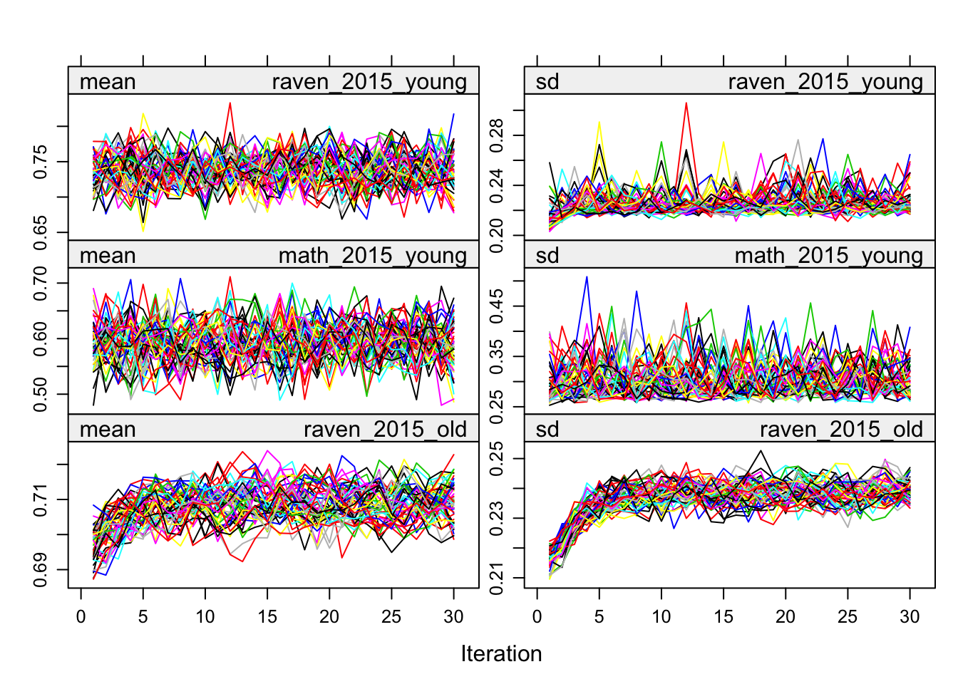
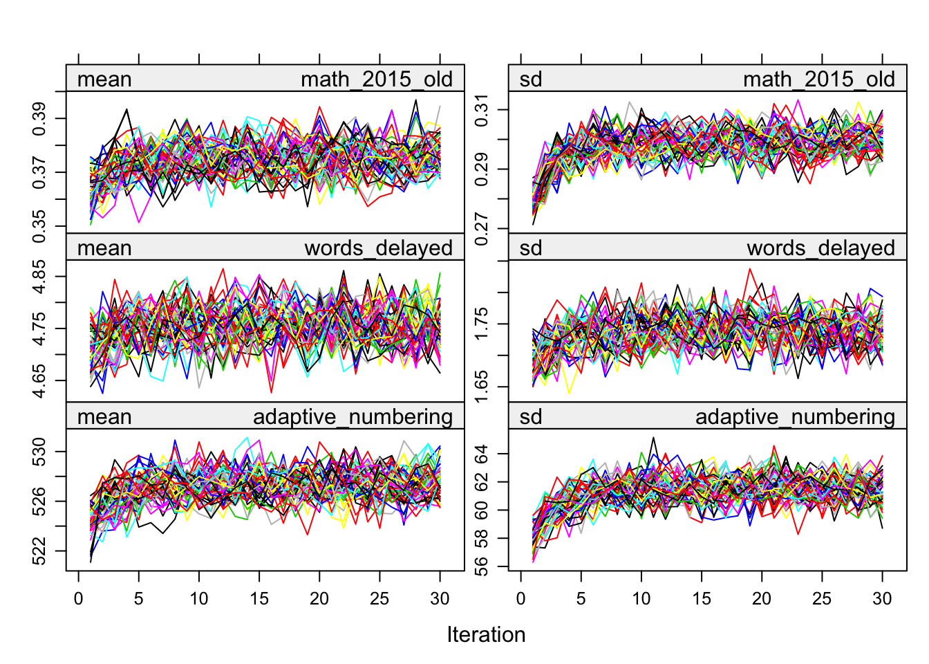
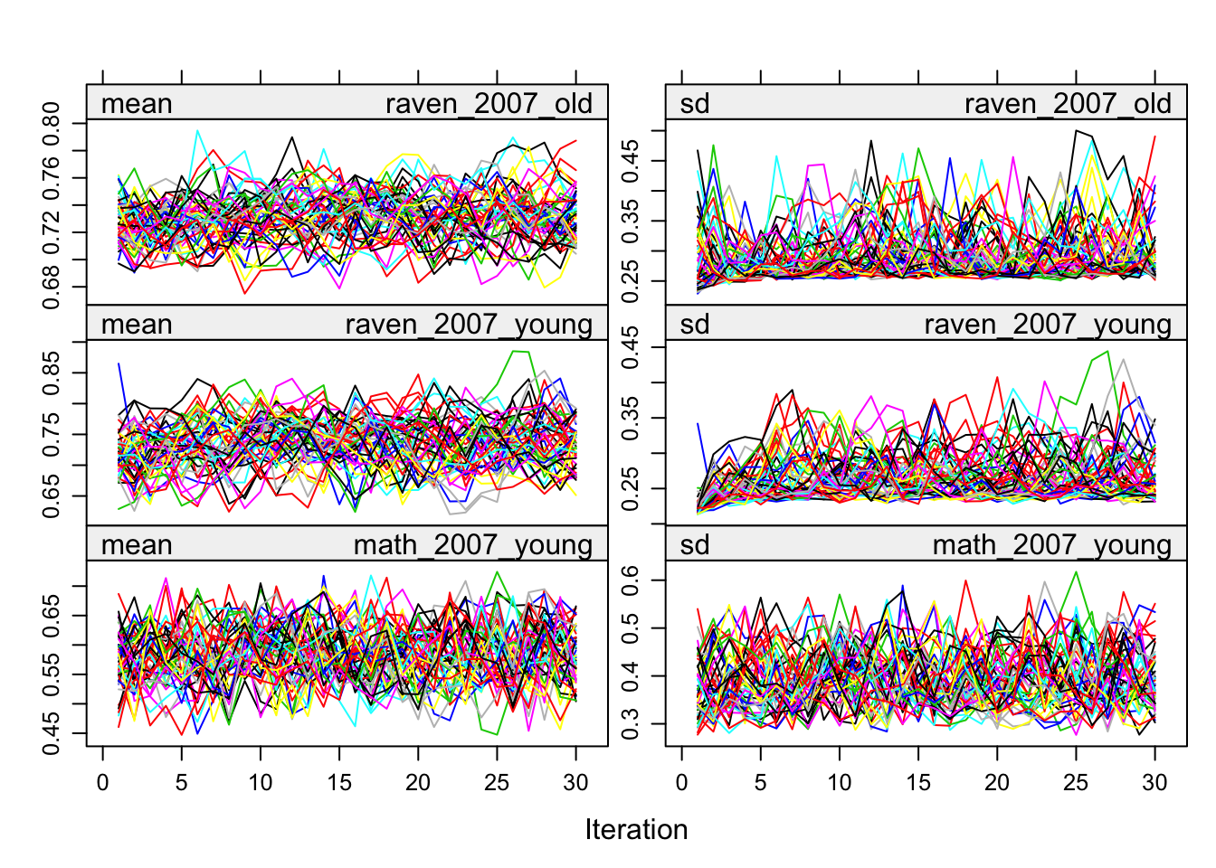
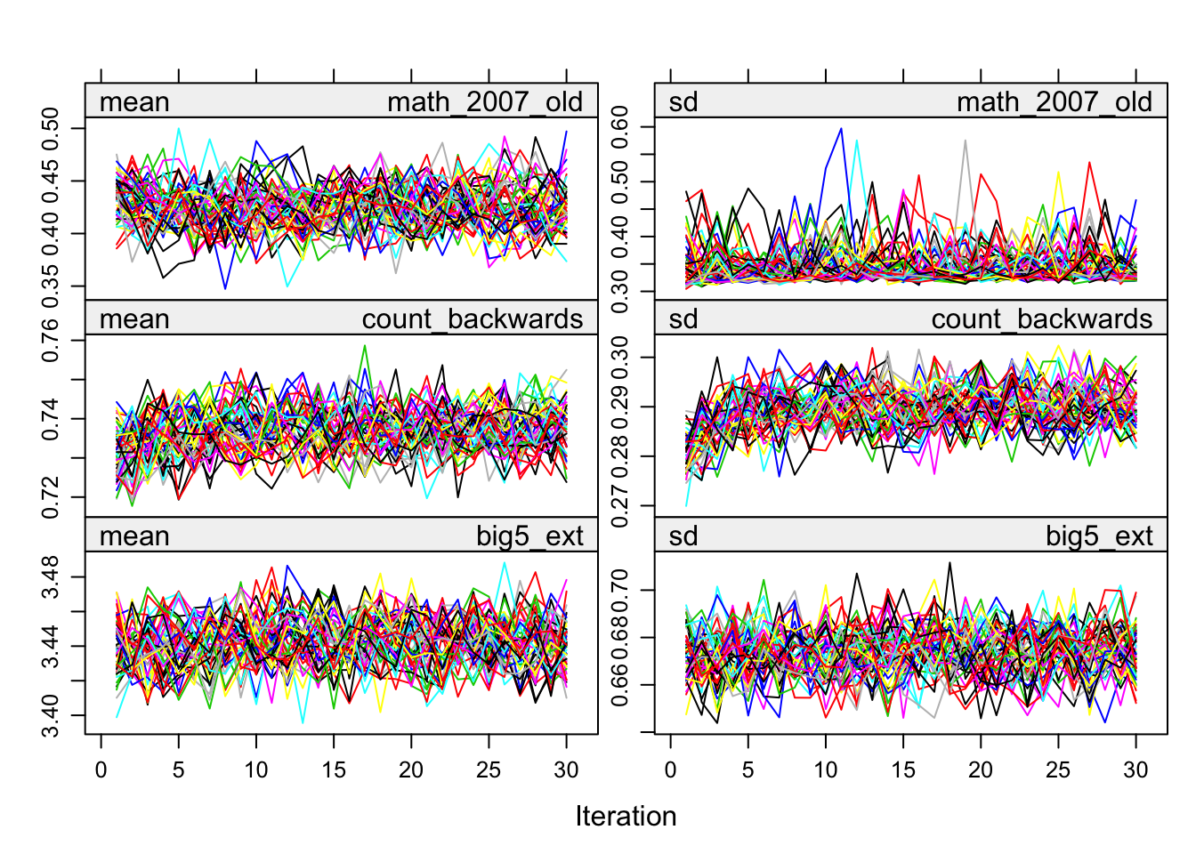
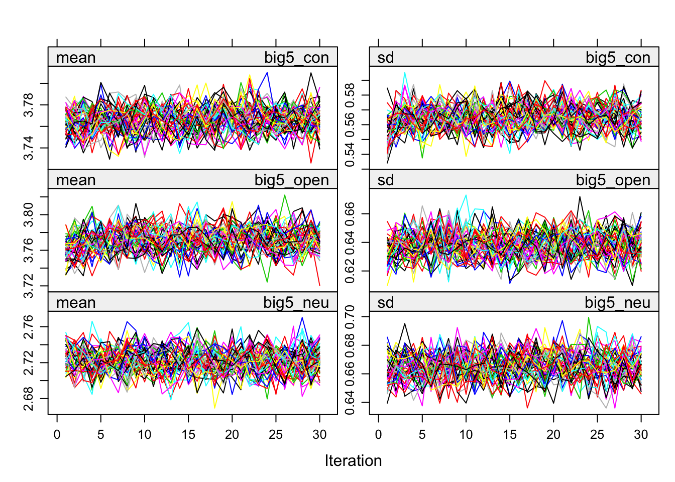
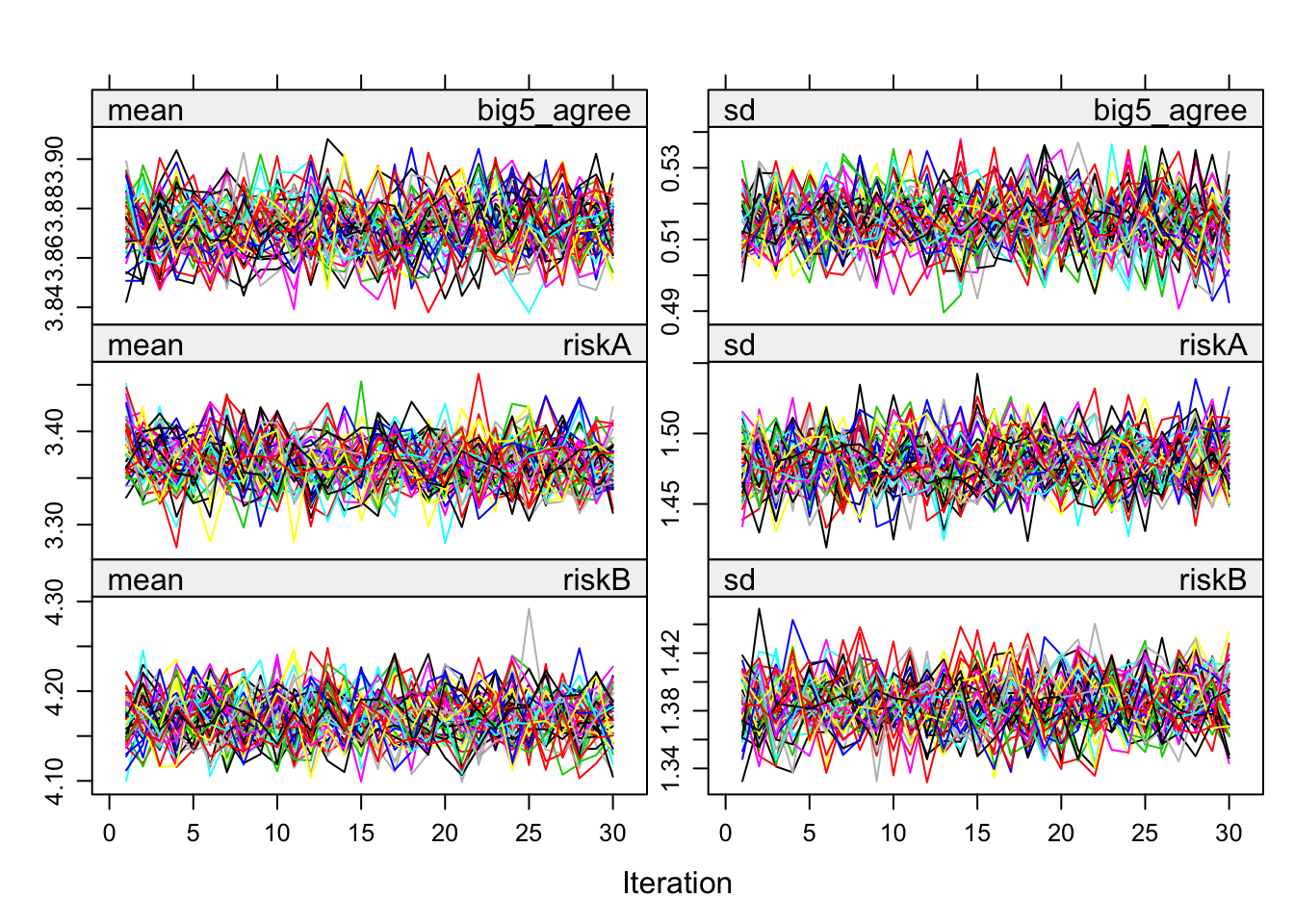
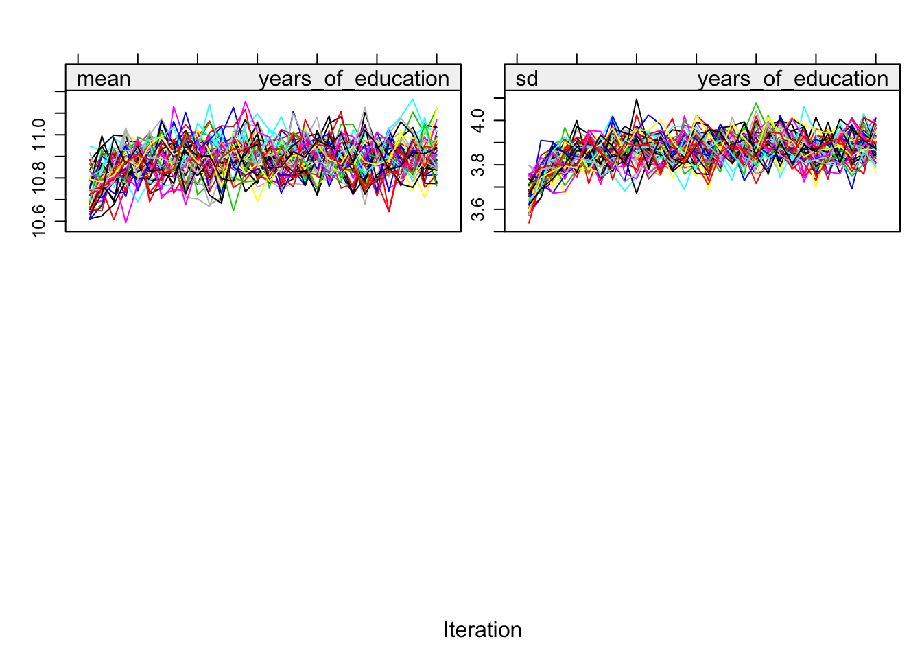
Iterations and convergence

plot(alldata_birthorder_i)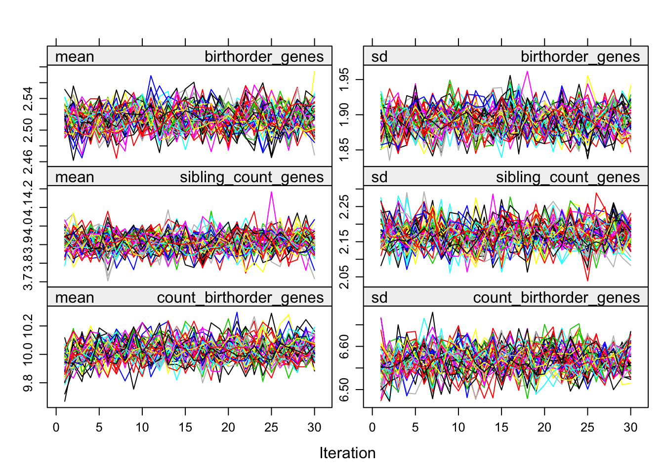

birthorder <- mids2mitml.list(alldata_birthorder_i)

Correlations, iterations and density

# correlations
correlations_original = corr_pipe(alldata_birthorder %>% select_if(is.numeric))
correlations_imputed = corr_pipe(alldata_birthorder_i_g_factor[[1]] %>% select_if(is.numeric))

correlations_original = correlations_original %>%
  mutate(v = paste0(Var1, Var2)) %>%
  rename(Var1_original = Var1, Var2_original= Var2, n_original = n, r_original = r, p_original = p)

correlations_imputed = correlations_imputed %>%
  mutate(v = paste0(Var1, Var2)) %>%
  rename(Var1_imputed = Var1, Var2_imputed = Var2, n_imputed = n, r_imputed = r, p_imputed = p)

correlations = full_join(correlations_original, correlations_imputed, by = "v")

cor.test(correlations$r_original, correlations$r_imputed)

Pearson’s product-moment correlation: correlations$r_original and correlations$r_imputed

Test statistic	df	P value	Alternative hypothesis	cor
64.09	700	4.117e-295 * * *	two.sided	0.9243

library(ggrepel)
sum(abs(correlations$r_original - correlations$r_imputed) > 0.5, na.rm = T)

## [1] 2

correlations <- correlations %>% 
  mutate(label = if_else(abs(r_original - r_imputed) > 0.4, 
                         paste(Var1_original, Var2_original),
                         NA_character_))
ggplot(correlations, aes(r_original, r_imputed)) +
  geom_point(alpha = 0.1) + 
  geom_text_repel(aes(label = label))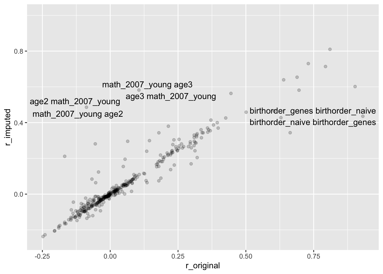

check densities of imputed/real

densityplot(alldata_birthorder_i, ~ birthorder_genes + sibling_count_genes)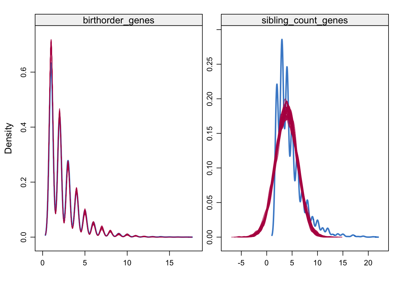

densityplot(alldata_birthorder_i, ~ raven_2015_young + math_2015_young + raven_2015_old + math_2015_old)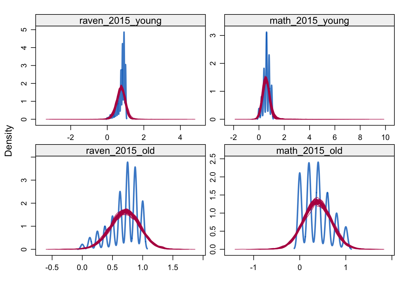

densityplot(alldata_birthorder_i, ~ words_delayed + adaptive_numbering + count_backwards)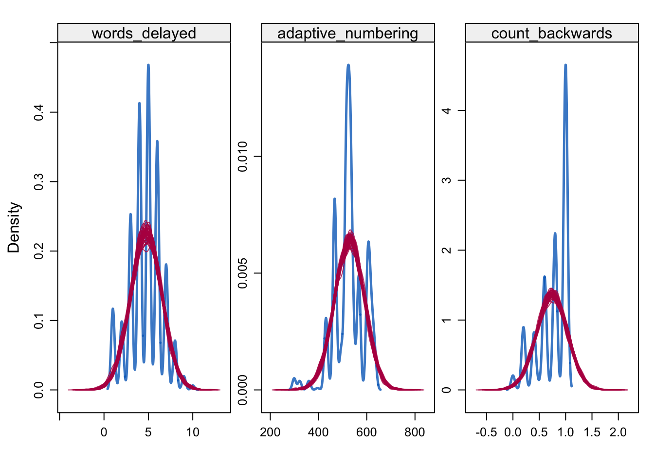

densityplot(alldata_birthorder_i, ~ raven_2007_old + raven_2007_young + math_2007_young + math_2007_old)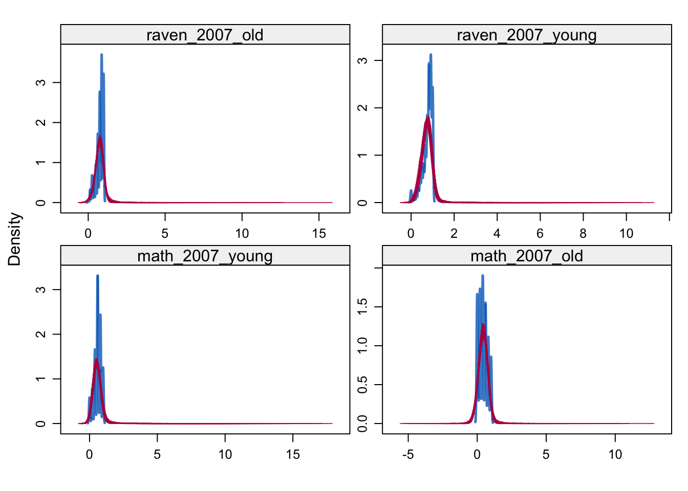

densityplot(alldata_birthorder_i, ~ big5_ext + big5_con + big5_open + big5_neu + big5_agree)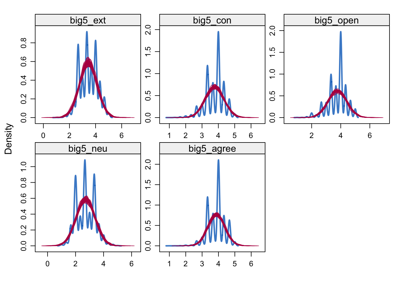

densityplot(alldata_birthorder_i, ~ riskA + riskB)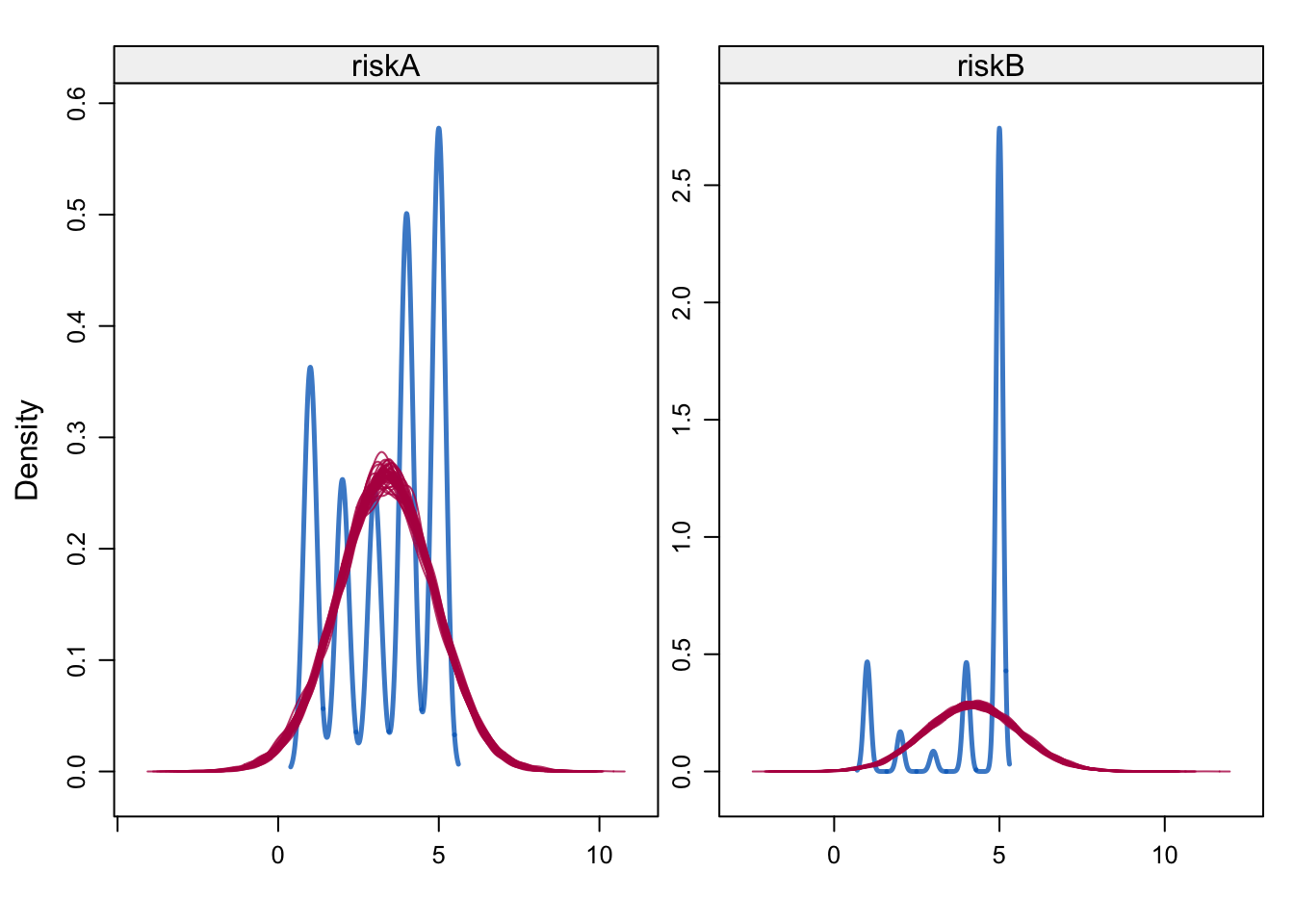

densityplot(alldata_birthorder_i, ~ years_of_education)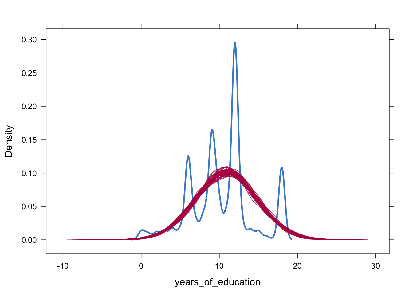

G-Factor

# Normal data - no misses
alldata_birthorder <- alldata_birthorder %>%
  mutate(pidlink = row_number())
no_miss = alldata_birthorder %>%
  filter(!is.na(raven_2015_old), !is.na(math_2015_old), !is.na(count_backwards),
         !is.na(words_delayed), !is.na(adaptive_numbering))
fa.parallel(no_miss %>% select(raven_2015_old, math_2015_old, count_backwards, words_delayed, adaptive_numbering) %>% data.frame())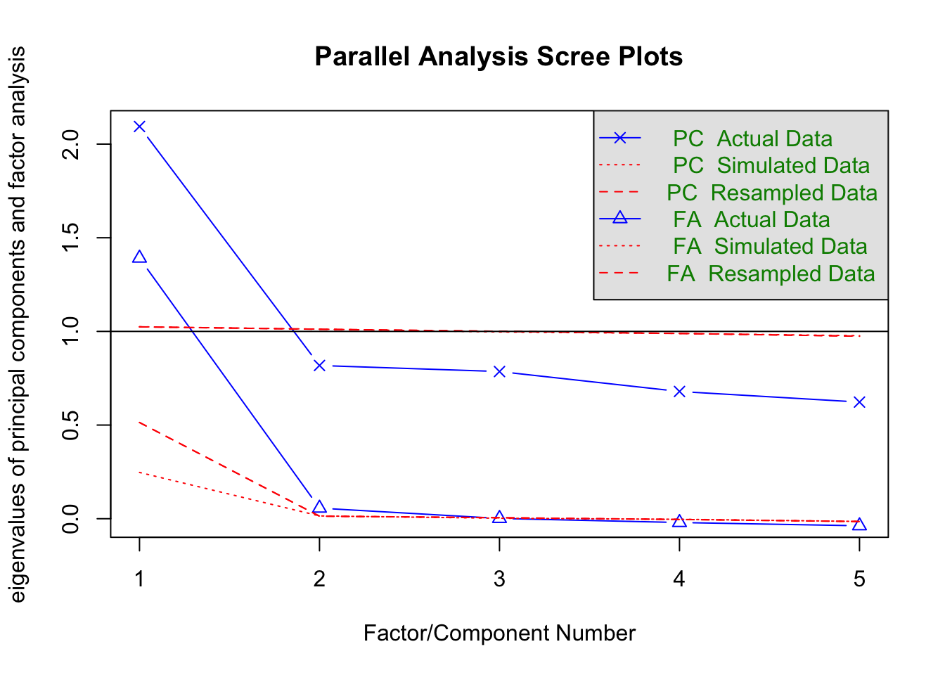

## Parallel analysis suggests that the number of factors =  2  and the number of components =  1

fa(no_miss %>% select(raven_2015_old, math_2015_old, count_backwards, words_delayed, adaptive_numbering) %>% data.frame(), nfactors = 1)

## Factor Analysis using method =  minres
## Call: fa(r = no_miss %>% select(raven_2015_old, math_2015_old, count_backwards, 
##     words_delayed, adaptive_numbering) %>% data.frame(), nfactors = 1)
## Standardized loadings (pattern matrix) based upon correlation matrix
##                     MR1   h2   u2 com
## raven_2015_old     0.60 0.36 0.64   1
## math_2015_old      0.51 0.26 0.74   1
## count_backwards    0.47 0.22 0.78   1
## words_delayed      0.41 0.17 0.83   1
## adaptive_numbering 0.61 0.38 0.62   1
## 
##                 MR1
## SS loadings    1.39
## Proportion Var 0.28
## 
## Mean item complexity =  1
## Test of the hypothesis that 1 factor is sufficient.
## 
## The degrees of freedom for the null model are  10  and the objective function was  0.56 with Chi Square of  7402
## The degrees of freedom for the model are 5  and the objective function was  0.01 
## 
## The root mean square of the residuals (RMSR) is  0.02 
## The df corrected root mean square of the residuals is  0.02 
## 
## The harmonic number of observations is  13151 with the empirical chi square  66.03  with prob <  6.8e-13 
## The total number of observations was  13151  with Likelihood Chi Square =  66.32  with prob <  6e-13 
## 
## Tucker Lewis Index of factoring reliability =  0.983
## RMSEA index =  0.031  and the 90 % confidence intervals are  0.024 0.037
## BIC =  18.9
## Fit based upon off diagonal values = 1
## Measures of factor score adequacy             
##                                                    MR1
## Correlation of (regression) scores with factors   0.82
## Multiple R square of scores with factors          0.67
## Minimum correlation of possible factor scores     0.34

om_results = omega(no_miss %>% select(raven_2015_old, math_2015_old, count_backwards, words_delayed, adaptive_numbering) %>% data.frame(), nfactors = 1, sl = F)

## Omega_h for 1 factor is not meaningful, just omega_t

om_results

## Omega 
## Call: omegah(m = m, nfactors = nfactors, fm = fm, key = key, flip = flip, 
##     digits = digits, title = title, sl = sl, labels = labels, 
##     plot = plot, n.obs = n.obs, rotate = rotate, Phi = Phi, option = option, 
##     covar = covar)
## Alpha:                 0.65 
## G.6:                   0.6 
## Omega Hierarchical:    0.65 
## Omega H asymptotic:    1 
## Omega Total            0.65 
## 
## Schmid Leiman Factor loadings greater than  0.2 
##                       g  F1*   h2   u2 p2
## raven_2015_old     0.60      0.36 0.64  1
## math_2015_old      0.51      0.26 0.74  1
## count_backwards    0.47      0.22 0.78  1
## words_delayed      0.41      0.17 0.83  1
## adaptive_numbering 0.61      0.38 0.62  1
## 
## With eigenvalues of:
##   g F1* 
## 1.4 0.0 
## 
## general/max  8354082811971781   max/min =   1
## mean percent general =  1    with sd =  0 and cv of  0 
## Explained Common Variance of the general factor =  1 
## 
## The degrees of freedom are 5  and the fit is  0.01 
## The number of observations was  13151  with Chi Square =  66.32  with prob <  6e-13
## The root mean square of the residuals is  0.02 
## The df corrected root mean square of the residuals is  0.02
## RMSEA index =  0.031  and the 10 % confidence intervals are  0.024 0.037
## BIC =  18.9
## 
## Compare this with the adequacy of just a general factor and no group factors
## The degrees of freedom for just the general factor are 5  and the fit is  0.01 
## The number of observations was  13151  with Chi Square =  66.32  with prob <  6e-13
## The root mean square of the residuals is  0.02 
## The df corrected root mean square of the residuals is  0.02 
## 
## RMSEA index =  0.031  and the 10 % confidence intervals are  0.024 0.037
## BIC =  18.9 
## 
## Measures of factor score adequacy             
##                                                  g F1*
## Correlation of scores with factors            0.82   0
## Multiple R square of scores with factors      0.67   0
## Minimum correlation of factor score estimates 0.34  -1
## 
##  Total, General and Subset omega for each subset
##                                                  g  F1*
## Omega total for total scores and subscales    0.65 0.65
## Omega general for total scores and subscales  0.65 0.65
## Omega group for total scores and subscales    0.00 0.00

omega.diagram(om_results)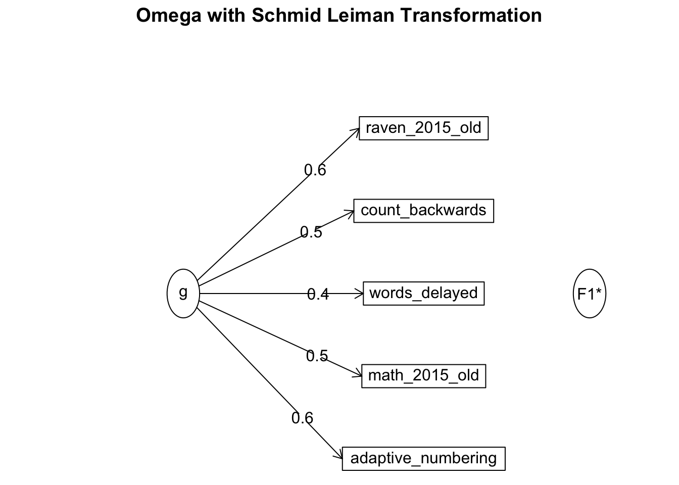

"g_factor_nomiss =~ raven_2015_old + math_2015_old + count_backwards +  words_delayed + adaptive_numbering" %>%
  cfa(data = no_miss, std.lv = T, std.ov = T) -> cfa_g
summary(cfa_g)

## lavaan 0.6-5 ended normally after 14 iterations
## 
##   Estimator                                         ML
##   Optimization method                           NLMINB
##   Number of free parameters                         10
##                                                       
##   Number of observations                         13151
##                                                       
## Model Test User Model:
##                                                       
##   Test statistic                                66.282
##   Degrees of freedom                                 5
##   P-value (Chi-square)                           0.000
## 
## Parameter Estimates:
## 
##   Information                                 Expected
##   Information saturated (h1) model          Structured
##   Standard errors                             Standard
## 
## Latent Variables:
##                      Estimate  Std.Err  z-value  P(>|z|)
##   g_factor_nomiss =~                                    
##     raven_2015_old      0.601    0.010   58.478    0.000
##     math_2015_old       0.512    0.010   49.908    0.000
##     count_backwrds      0.475    0.010   46.155    0.000
##     words_delayed       0.408    0.010   39.376    0.000
##     adaptiv_nmbrng      0.614    0.010   59.659    0.000
## 
## Variances:
##                    Estimate  Std.Err  z-value  P(>|z|)
##    .raven_2015_old    0.639    0.011   57.294    0.000
##    .math_2015_old     0.738    0.011   66.322    0.000
##    .count_backwrds    0.775    0.011   69.060    0.000
##    .words_delayed     0.834    0.011   72.907    0.000
##    .adaptiv_nmbrng    0.623    0.011   55.665    0.000
##     g_factor_nomss    1.000

## Explained variance:
x = inspect(cfa_g, "rsquare")
no_miss$g_factor_nomiss = predict(cfa_g)[,1]

no_miss = no_miss %>% select(pidlink, g_factor_nomiss)

alldata_birthorder = left_join(alldata_birthorder, no_miss, by = "pidlink")
qplot(alldata_birthorder$g_factor_nomiss)

## `stat_bin()` using `bins = 30`. Pick better value with `binwidth`.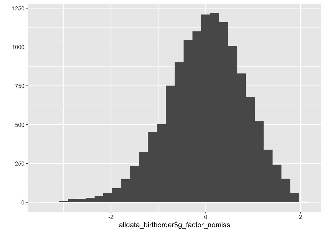

qplot(alldata_birthorder_i_g_factor[[1]]$g_factor_2015)

## `stat_bin()` using `bins = 30`. Pick better value with `binwidth`.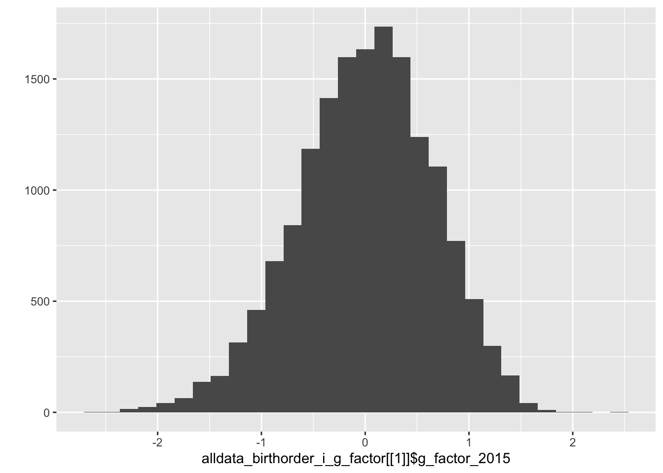

qplot(alldata_birthorder_i_g_factor[[1]]$g_factor_2007)

## `stat_bin()` using `bins = 30`. Pick better value with `binwidth`.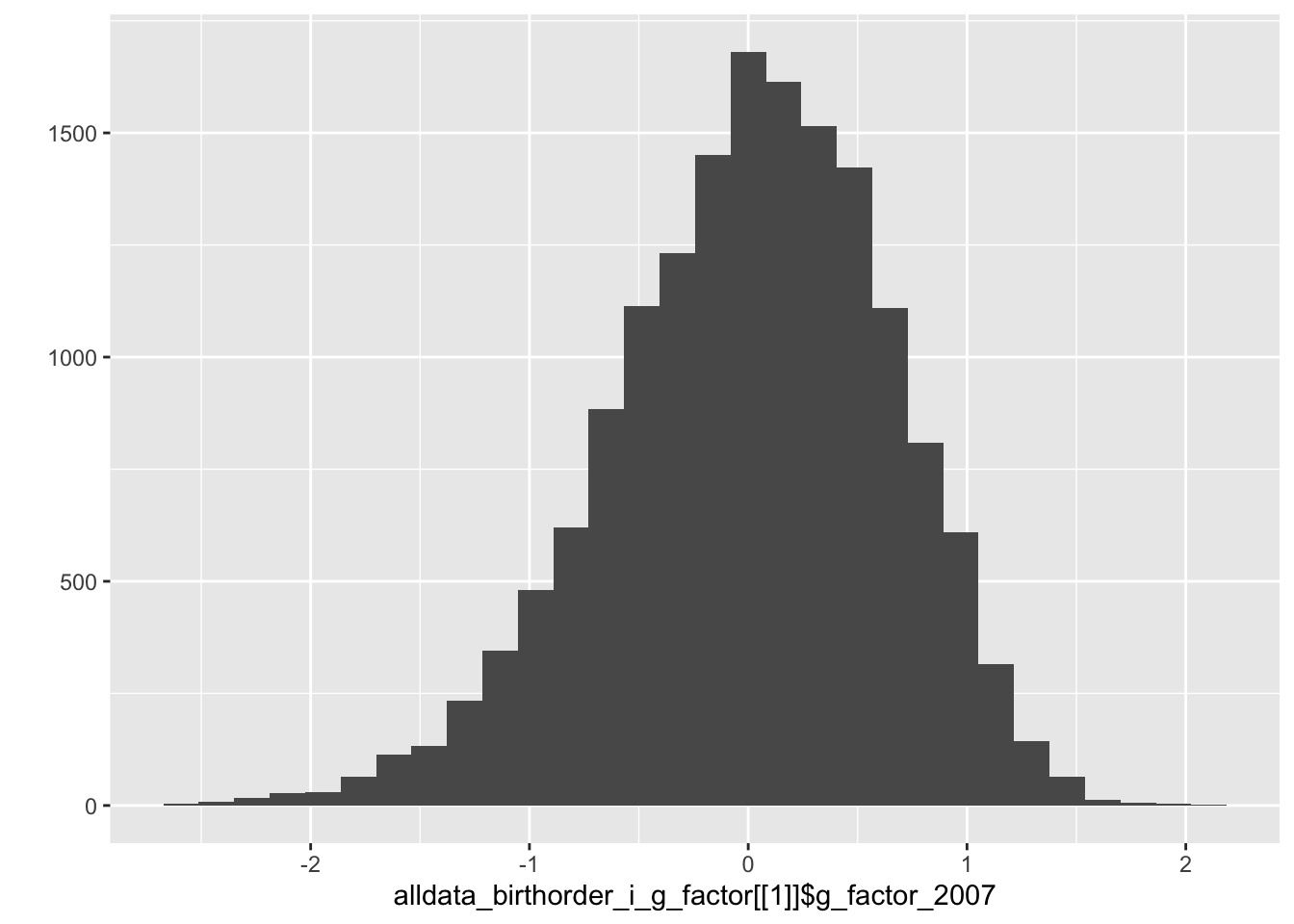

summary(lm(g_factor_nomiss ~ raven_2015_old, alldata_birthorder))

Estimate	Std. Error	t value	Pr(>|t|)
-1.795	0.01523	-117.8	0
2.569	0.02068	124.2	0

Fitting linear model: g_factor_nomiss ~ raven_2015_old

Observations	Residual Std. Error	\(R^2\)	Adjusted \(R^2\)
13151	0.5545	0.54	0.5399

summary(lm(g_factor_2015 ~ raven_2015_old, alldata_birthorder_i_g_factor[[1]]))

Estimate	Std. Error	t value	Pr(>|t|)
-3.129e-15	0.003715	-8.423e-13	1
0.4553	0.003715	122.6	0

Fitting linear model: g_factor_2015 ~ raven_2015_old

Observations	Residual Std. Error	\(R^2\)	Adjusted \(R^2\)
16063	0.4708	0.4833	0.4833

summary(lm(g_factor_nomiss ~ raven_2015_young, alldata_birthorder))

Estimate	Std. Error	t value	Pr(>|t|)
-1.459	0.03528	-41.35	9.881e-324
2.129	0.04343	49.02	0

Fitting linear model: g_factor_nomiss ~ raven_2015_young

Observations	Residual Std. Error	\(R^2\)	Adjusted \(R^2\)
5250	0.6195	0.3141	0.314

summary(lm(g_factor_2015 ~ raven_2015_young, alldata_birthorder_i_g_factor[[1]]))

Estimate	Std. Error	t value	Pr(>|t|)
-1.199e-15	0.004378	-2.739e-13	1
0.3479	0.004378	79.46	0

Fitting linear model: g_factor_2015 ~ raven_2015_young

Observations	Residual Std. Error	\(R^2\)	Adjusted \(R^2\)
16063	0.5549	0.2822	0.2821

alldata_birthorder %>% {cor.test(.$g_factor_nomiss, .$years_of_education)}

Pearson’s product-moment correlation: .$g_factor_nomiss and .$years_of_education

Test statistic	df	P value	Alternative hypothesis	cor
60.48	12922	0 * * *	two.sided	0.4697

alldata_birthorder_i_g_factor[[1]] %>% {cor.test(.$g_factor_2015, .$years_of_education)}

Pearson’s product-moment correlation: .$g_factor_2015 and .$years_of_education

Test statistic	df	P value	Alternative hypothesis	cor
70.52	16061	0 * * *	two.sided	0.4862

alldata_birthorder_i_g_factor[[1]] %>% {cor.test(.$g_factor_2007, .$years_of_education)}

Pearson’s product-moment correlation: .$g_factor_2007 and .$years_of_education

Test statistic	df	P value	Alternative hypothesis	cor
71.34	16061	0 * * *	two.sided	0.4906

alldata_birthorder_i_g_factor[[1]] %>% {cor.test(.$g_factor_2007, .$g_factor_2015)}

Pearson’s product-moment correlation: .$g_factor_2007 and .$g_factor_2015

Test statistic	df	P value	Alternative hypothesis	cor
209.2	16061	0 * * *	two.sided	0.8553