Codebook

source("0_helpers.R")
birthorder = readRDS("data/alldata_birthorder.rds")
knitr::opts_chunk$set(error = TRUE, warning = F, message = F)

Data

# For analyses we want to clean the dataset and get rid of all uninteresting data
birthorder = birthorder %>%
 mutate(money_spent_smoking_log = if_else(is.na(money_spent_smoking_log) & ever_smoked == 0, 0, money_spent_smoking_log),
         amount = if_else(is.na(amount) & ever_smoked == 0, 0, amount),
         amount_still_smokers = if_else(is.na(amount_still_smokers) &  still_smoking == 0, 0, amount_still_smokers),
         birthyear = lubridate::year(birthdate))

### Variables
birthorder = birthorder %>%
  mutate(
  attended_school = as.integer(attended_school),
  attended_school = ifelse(attended_school == 1, 0,
                           ifelse(attended_school == 2, 1, NA)))

### Birthorder and Sibling Count
birthorder = birthorder %>% 
  mutate(
# birthorder as factors with levels of 1, 2, 3, 4, 5, >5
    birthorder_naive_factor = as.character(birthorder_naive),
    birthorder_naive_factor = ifelse(birthorder_naive > 5, ">5",
                                            birthorder_naive_factor),
    birthorder_naive_factor = factor(birthorder_naive_factor, 
                                            levels = c("1","2","3","4","5",">5")),
    sibling_count_naive_factor = as.character(sibling_count_naive),
    sibling_count_naive_factor = ifelse(sibling_count_naive > 5, ">5",
                                               sibling_count_naive_factor),
    sibling_count_naive_factor = factor(sibling_count_naive_factor, 
                                               levels = c("2","3","4","5",">5")),

    birthorder_uterus_alive_factor = as.character(birthorder_uterus_alive),
    birthorder_uterus_alive_factor = ifelse(birthorder_uterus_alive > 5, ">5",
                                            birthorder_uterus_alive_factor),
    birthorder_uterus_alive_factor = factor(birthorder_uterus_alive_factor, 
                                            levels = c("1","2","3","4","5",">5")),
    sibling_count_uterus_alive_factor = as.character(sibling_count_uterus_alive),
    sibling_count_uterus_alive_factor = ifelse(sibling_count_uterus_alive > 5, ">5",
                                               sibling_count_uterus_alive_factor),
    sibling_count_uterus_alive_factor = factor(sibling_count_uterus_alive_factor, 
                                               levels = c("2","3","4","5",">5")),
    birthorder_uterus_preg_factor = as.character(birthorder_uterus_preg),
    birthorder_uterus_preg_factor = ifelse(birthorder_uterus_preg > 5, ">5",
                                           birthorder_uterus_preg_factor),
    birthorder_uterus_preg_factor = factor(birthorder_uterus_preg_factor,
                                           levels = c("1","2","3","4","5",">5")),
    sibling_count_uterus_preg_factor = as.character(sibling_count_uterus_preg),
    sibling_count_uterus_preg_factor = ifelse(sibling_count_uterus_preg > 5, ">5",
                                              sibling_count_uterus_preg_factor),
    sibling_count_uterus_preg_factor = factor(sibling_count_uterus_preg_factor, 
                                              levels = c("2","3","4","5",">5")),
    birthorder_genes_factor = as.character(birthorder_genes),
    birthorder_genes_factor = ifelse(birthorder_genes >5 , ">5", birthorder_genes_factor),
    birthorder_genes_factor = factor(birthorder_genes_factor, 
                                     levels = c("1","2","3","4","5",">5")),
    sibling_count_genes_factor = as.character(sibling_count_genes),
    sibling_count_genes_factor = ifelse(sibling_count_genes >5 , ">5",
                                        sibling_count_genes_factor),
    sibling_count_genes_factor = factor(sibling_count_genes_factor, 
                                        levels = c("2","3","4","5",">5")),
    # interaction birthorder * siblingcout for each birthorder
    count_birthorder_naive =
      factor(str_replace(as.character(interaction(birthorder_naive_factor,                                                              sibling_count_naive_factor)),
                        "\\.", "/"),
                                           levels =   c("1/2","2/2", "1/3",  "2/3",
                                                        "3/3", "1/4", "2/4", "3/4", "4/4",
                                                        "1/5", "2/5", "3/5", "4/5", "5/5",
                                                        "1/>5", "2/>5", "3/>5", "4/>5",
                                                        "5/>5", ">5/>5")),
    count_birthorder_uterus_alive =
      factor(str_replace(as.character(interaction(birthorder_uterus_alive_factor,                                                              sibling_count_uterus_alive_factor)),
                        "\\.", "/"),
                                           levels =   c("1/2","2/2", "1/3",  "2/3",
                                                        "3/3", "1/4", "2/4", "3/4", "4/4",
                                                        "1/5", "2/5", "3/5", "4/5", "5/5",
                                                        "1/>5", "2/>5", "3/>5", "4/>5",
                                                        "5/>5", ">5/>5")),
    count_birthorder_uterus_preg =
      factor(str_replace(as.character(interaction(birthorder_uterus_preg_factor,                                                              sibling_count_uterus_preg_factor)), 
                         "\\.", "/"),
                                           levels =   c("1/2","2/2", "1/3",  "2/3",
                                                        "3/3", "1/4", "2/4", "3/4", "4/4",
                                                        "1/5", "2/5", "3/5", "4/5", "5/5",
                                                        "1/>5", "2/>5", "3/>5", "4/>5",
                                                        "5/>5", ">5/>5")),
    count_birthorder_genes =
      factor(str_replace(as.character(interaction(birthorder_genes_factor,                                                              sibling_count_genes_factor)), "\\.", "/"),
                                           levels =   c("1/2","2/2", "1/3",  "2/3",
                                                        "3/3", "1/4", "2/4", "3/4", "4/4",
                                                        "1/5", "2/5", "3/5", "4/5", "5/5",
                                                        "1/>5", "2/>5", "3/>5", "4/>5",
                                                        "5/>5", ">5/>5")))

birthorder <- birthorder %>%
                     mutate(sibling_count = sibling_count_naive_factor,
                            birth_order_nonlinear = birthorder_naive_factor,
                            birth_order = birthorder_naive,
                            count_birth_order = count_birthorder_naive)

birthorder$mother_pidlink <- as.character(birthorder$mother_pidlink)
birthorder$pidlink <- as.character(birthorder$pidlink)
birthorder$father_pidlink <- as.character(birthorder$father_pidlink)
birthorder$marriage_id <- as.character(birthorder$marriage_id)
library(codebook)

var_label(birthorder$e1) <- "Is talkative"
var_label(birthorder$c1) <- "Does a thorough job"
var_label(birthorder$o1) <- "Is original, comes up with new ideas."
var_label(birthorder$e2r_reversed) <- "Is reserved."
var_label(birthorder$n1r_reversed) <- "Is relaxed, handles stress well."
var_label(birthorder$a1) <- "Has a forgiving nature."
var_label(birthorder$n2) <- "Worries a lot."
var_label(birthorder$o2) <- "Has an active imagination."
var_label(birthorder$c2r_reversed) <- "Tends to be lazy."
var_label(birthorder$o3) <- "Values artistic, aesthetic experiences."
var_label(birthorder$a2) <- "Is considerate and kind to almost everyone."
var_label(birthorder$c3) <- "Does things efficiently."
var_label(birthorder$e3) <- "Outgoing, sociable."
var_label(birthorder$a3r_reversed) <- "Is sometimes rude to others."
var_label(birthorder$n3) <- "Gets nervous easily."



add_likert_labels <- function(x) {
  val_labels(x) <- c("Disagree strongly" = 1, 
                  "Disagree a little" = 2, 
                  "Neither agree nor disagree" = 3,
                  "Agree a little" = 4,
                  "Agree strongly" = 5)
  x
}
birthorder <- birthorder %>% mutate_at(vars(e1, c1, o1, e2r, n1r, a1, n2, o2, c2r, o3, a2, c3, e3, a3r, n3), add_likert_labels)

##Extraversion
birthorder$e2r_reversed = codebook::reverse_labelled_values(birthorder$e2r)
extraversion = birthorder %>% select(e1, e2r_reversed, e3)
birthorder$big5_ext = aggregate_and_document_scale(extraversion)

##conscientiousness
birthorder$c2r_reversed = codebook::reverse_labelled_values(birthorder$c2r)
conscientiousness = birthorder %>% select(c1, c2r_reversed, c3)
birthorder$big5_con = aggregate_and_document_scale(conscientiousness)

##Openness
openness = birthorder %>% select(o1, o2, o3)
birthorder$big5_open = aggregate_and_document_scale(openness)

## Neuroticism
birthorder$n1r_reversed = codebook::reverse_labelled_values(birthorder$n1r)
neuroticism = birthorder %>% select(n1r_reversed, n2, n3)
birthorder$big5_neu = aggregate_and_document_scale(neuroticism)

##Agreeableness
birthorder$a3r_reversed = codebook::reverse_labelled_values(birthorder$a3r)
agreeableness= birthorder %>% select(a1, a2, a3r_reversed)
birthorder$big5_agree = aggregate_and_document_scale(agreeableness)

cb_table <- codebook_table(birthorder)
rio::export(cb_table, "2_codebook.xlsx")

metadata(birthorder)$name <- "Indonesian Family Life Study, merged subset"
metadata(birthorder)$description <- "Data from the IFLS, merged across waves, most outcomes taken from wave 5. Includes birth order, family structure, Big 5 Personality, intelligence tests, and risk lotteries"
metadata(birthorder)$identifier <- "https://www.rand.org/well-being/social-and-behavioral-policy/data/FLS/IFLS.html"
metadata(birthorder)$creator <- "RAND corporation"
metadata(birthorder)$citation <- "Strauss, J., Witoelar, F., & Sikoki, B. (2016). The Fifth Wave of the Indonesia Family Life Survey: Overview and Field Report. WR-1143/1-NIA/NICHD"
metadata(birthorder)$url <- "https://www.rand.org/well-being/social-and-behavioral-policy/data/FLS/IFLS.html"
metadata(birthorder)$datePublished <- "2016"
metadata(birthorder)$temporalCoverage <- "2014/2015" 
metadata(birthorder)$spatialCoverage <- "13 Indonesian provinces. The sample is representative of about 83% of the Indonesian population and contains over 30,000 individuals living in 13 of the 27 provinces in the country. See URL for more." 

codebook(birthorder, survey_repetition = "single", 
        detailed_variables = FALSE, detailed_scales = TRUE, missingness_report = FALSE,
        metadata_table = TRUE, metadata_json = TRUE, indent = "#")

knitr::asis_output(data_info)

Metadata

Description

if (exists("name", meta)) {
  glue::glue(
    "__Dataset name__: {name}",
    .envir = meta)
}

Dataset name: Indonesian Family Life Study, merged subset

cat(description)

Data from the IFLS, merged across waves, most outcomes taken from wave 5. Includes birth order, family structure, Big 5 Personality, intelligence tests, and risk lotteries

Metadata for search engines

• Temporal Coverage: 2014/2015
• Spatial Coverage: 13 Indonesian provinces. The sample is representative of about 83% of the Indonesian population and contains over 30,000 individuals living in 13 of the 27 provinces in the country. See URL for more.
• Citation: Strauss, J., Witoelar, F., & Sikoki, B. (2016). The Fifth Wave of the Indonesia Family Life Survey: Overview and Field Report. WR-1143/1-NIA/NICHD
• URL: https://www.rand.org/well-being/social-and-behavioral-policy/data/FLS/IFLS.html
• Identifier: https://www.rand.org/well-being/social-and-behavioral-policy/data/FLS/IFLS.html

• Date published: 2016

• Creator:RAND corporation

meta <- meta[setdiff(names(meta),
                     c("creator", "datePublished", "identifier",
                       "url", "citation", "spatialCoverage", 
                       "temporalCoverage", "description", "name"))]
pander::pander(meta)

• keywords: wave, mother_pidlink, chron_order_birth, lifebirths, multiple_birth, alive, birthdate, any_multiple_birth, marriage_id, birthorder_uterus_preg, sibling_count_uterus_preg, birthorder_uterus_alive, sibling_count_uterus_alive, birthorder_genes, sibling_count_genes, pidlink, father_pidlink, age, death_yr, death_month, sc05, province, sc01_14_14, sibling_count_naive_ind, any_multiple_birthdate, birthorder_naive, sibling_count_naive, age_2015_old, age_2015_young, raven_2015_young, math_2015_young, raven_2015_old, math_2015_old, words_immediate, words_delayed, words_remembered_avg, adaptive_numbering, age_2007_young, age_2007_old, raven_2007_old, raven_2007_young, math_2007_young, math_2007_old, count_backwards, g_factor_2015_old, g_factor_2015_young, g_factor_2007_old, g_factor_2007_young, e1, c1, o1, e2r, n1r, a1, n2, o2, c2r, o3, a2, c3, e3, a3r, n3, e2r_reversed, big5_ext, c2r_reversed, big5_con, big5_open, n1r_reversed, big5_neu, a3r_reversed, big5_agree, random_si, si01, si02, si03, si04, si05, si11, si12, si13, si14, si15, riskA, riskB, attended_school, highest_education, currently_attending_school, hours_in_class, years_of_education, Type_of_test_elementary, Indonesia_score_elementary, English_score_elementary, Math_score_elemenatry, Total_score_elemenatry, Type_of_test_Junior_High, Indonesia_score_Junior_High, English_score_Junior_High, Math_score_Junior_High, Total_score_Junior_High, Type_of_test_Senior_High, Indonesia_score_Senior_High, English_score_Senior_High, Math_score_Senior_High, Total_score_Senior_High, Total_score_highest, Total_score_highest_type, Math_score_highest, Math_score_highest_type, Elementary_worked, Junior_high_worked, Senior_high_worked, University_worked, total_worked, Elementary_missed, Junior_high_missed, Senior_high_missed, University_missed, total_missed, Category, Sector, Self_employed, ever_smoked, still_smoking, amount, age_first_smoke, amount_still_smokers, male, wage_last_month_log, wage_last_year_log, money_spent_smoking_log, birthyear, birthorder_naive_factor, sibling_count_naive_factor, birthorder_uterus_alive_factor, sibling_count_uterus_alive_factor, birthorder_uterus_preg_factor, sibling_count_uterus_preg_factor, birthorder_genes_factor, sibling_count_genes_factor, count_birthorder_naive, count_birthorder_uterus_alive, count_birthorder_uterus_preg, count_birthorder_genes, sibling_count, birth_order_nonlinear, birth_order and count_birth_order

knitr::asis_output(survey_overview)

Variables

if (detailed_variables || detailed_scales) {
  knitr::asis_output(paste0(scales_items, sep = "\n\n\n", collapse = "\n\n\n"))
}

Scale: big5_ext

Overview

Reliability: ω_ordinal [95% CI] = 0.59 [0.52;0.65].

Missing: 69795.

old_height <- knitr::opts_chunk$get("fig.height")
new_height <- length(scale_info$scale_item_names)
new_height <- ifelse(new_height > 20, 20, new_height)
new_height <- ifelse(new_height < 1, 1, new_height)
new_height <- ifelse(is.na(new_height) | is.nan(new_height), 
                     old_height, new_height)
knitr::opts_chunk$set(fig.height = new_height)

if (dplyr::n_distinct(na.omit(unlist(items))) < 12) {
  likert_plot <- likert_from_items(items)
  if (!is.null(likert_plot)) {
    graphics::plot(likert_plot)
  }
}

knitr::opts_chunk$set(fig.height = old_height)

wrap_at <- knitr::opts_chunk$get("fig.width") * 10

dist_plot <- plot_labelled(scale, scale_name, wrap_at)

choices <- attributes(items[[1]])$item$choices
breaks <- as.numeric(names(choices))
if (length(breaks)) {
  suppressMessages( # ignore message about overwriting x axis
  dist_plot <- dist_plot +
        ggplot2::scale_x_continuous("values", 
                                breaks = breaks, 
                                labels = stringr::str_wrap(unlist(choices), ceiling(wrap_at * 0.21))) +
      ggplot2::expand_limits(x = range(breaks)))
  
}

dist_plot

Reliability details

for (i in seq_along(reliabilities)) {
  rel <- reliabilities[[i]]
  cat(knitr::knit_print(rel, indent = paste0(indent, "####")))
}

Reliability Indices

coefs <- x$scaleReliability$output$dat %>% 
  tidyr::gather(index, estimate) %>% 
  dplyr::filter(index != "n.items", index != "n.observations") %>% 
  dplyr::mutate(index = stringr::str_to_title(
    stringr::str_replace_all(index,
      stringr::fixed("."), " ")))

cis <- coefs %>% 
  dplyr::filter(stringr::str_detect(index, " Ci ")) %>% 
  tidyr::separate(index, c("index", "hilo"), sep = " Ci ") %>% 
  tidyr::spread(hilo, estimate)
if (nrow(cis)) {
  cis <- cis %>% dplyr::rename(
    `Lower 95% CI` = .data$Lo, `Upper 95% CI` = .data$Hi
  )
}

coefs_with_cis <- coefs %>% 
  dplyr::filter(!stringr::str_detect(index, " Ci ")) %>% 
    dplyr::left_join(cis, by = "index") %>% 
    dplyr::mutate(index = dplyr::if_else(index == "Glb", "Greatest Lower Bound", .data$index)) %>% 
    dplyr::arrange(!stringr::str_detect(index, "Omega")) %>% 
    dplyr::select(Index = .data$index, Estimate = .data$estimate)


pander::pander(coefs_with_cis)

Index	Estimate
Omega	0.5702
Omega Psych Tot	0.2915
Omega Psych H	0.001267
Omega Ordinal	0.5862
Cronbach Alpha	0.3679
Greatest Lower Bound	0.4454
Alpha Ordinal	0.385

Positive correlations: 3 out of 3 (100%)

Scatter matrix

print(x$scatterMatrix$output$scatterMatrix)

x$scatterMatrix$output$scatterMatrix <- no_md()

Detailed output

print(x)

## 
## Information about this analysis:
## 
##                  Dataframe: res$dat
##                      Items: e1, e2r_reversed, e3
##               Observations: 31446
##      Positive correlations: 3 out of 3 (100%)
## 
## Estimates assuming interval level:
## 
##              Omega (total): 0.57
##       Omega (hierarchical): 0
##    Revelle's omega (total): 0.29
## Greatest Lower Bound (GLB): 0.45
##              Coefficient H: 0.91
##           Cronbach's alpha: 0.37
## Confidence intervals:
##              Omega (total): [0.5, 0.64]
##           Cronbach's alpha: [0.36, 0.38]
## 
## Estimates assuming ordinal level:
## 
##      Ordinal Omega (total): 0.59
##  Ordinal Omega (hierarch.): 0.59
##   Ordinal Cronbach's alpha: 0.38
## Confidence intervals:
##      Ordinal Omega (total): [0.52, 0.65]
##   Ordinal Cronbach's alpha: [0.37, 0.4]
## 
## Note: the normal point estimate and confidence interval for omega are based on the procedure suggested by Dunn, Baguley & Brunsden (2013) using the MBESS function ci.reliability, whereas the psych package point estimate was suggested in Revelle & Zinbarg (2008). See the help ('?scaleStructure') for more information.
## 
## Eigen values: 1.326, 0.966, 0.708
## Loadings:
##              PC1  
## e1           0.789
## e2r_reversed 0.718
## e3           0.433
## 
##                  PC1
## SS loadings    1.326
## Proportion Var 0.442
## 
##              vars     n mean   sd median trimmed  mad min max range  skew kurtosis   se
## e1              1 31446 3.15 1.14      3    3.09 1.48   1   5     4  0.02    -1.37 0.01
## e2r_reversed    2 31446 3.02 1.12      3    3.06 1.48   1   5     4 -0.16    -1.30 0.01
## e3              3 31446 4.16 0.67      4    4.22 0.00   1   5     4 -1.09     3.25 0.00

Summary statistics

for (i in seq_along(names(items))) {
  attributes(items[[i]]) = recursive_escape(attributes(items[[i]]))
}
escaped_table(codebook_table(items))

## 
## 
## name           label                 data_type        value_labels                                                                                                                   n_missing   complete_rate  min   median   max     mean       sd   n_value_labels  hist     
## -------------  --------------------  ---------------  ----------------------------------------------------------------------------------------------------------------------------  ----------  --------------  ----  -------  ----  ------  -------  ---------------  ---------
## e1             Is talkative          haven_labelled   1. Disagree strongly,<br>2. Disagree a little,<br>3. Neither agree nor disagree,<br>4. Agree a little,<br>5. Agree strongly        69795          0.3106  1     3        5      3.146   1.1437                5  ▁▇▁▂▁▇▁▂ 
## e2r_reversed   NA                    haven_labelled   5. Disagree strongly,<br>4. Disagree a little,<br>3. Neither agree nor disagree,<br>2. Agree a little,<br>1. Agree strongly        69795          0.3106  1     3        5      3.019   1.1246                5  ▂▆▁▂▁▇▁▁ 
## e3             Outgoing, sociable.   haven_labelled   1. Disagree strongly,<br>2. Disagree a little,<br>3. Neither agree nor disagree,<br>4. Agree a little,<br>5. Agree strongly        69795          0.3106  1     4        5      4.162   0.6687                5  ▁▁▁▁▁▇▁▃

Scale: big5_con

Overview

Reliability: ω_ordinal [95% CI] = 0.46 [0.45;0.47].

Missing: 69795.

old_height <- knitr::opts_chunk$get("fig.height")
new_height <- length(scale_info$scale_item_names)
new_height <- ifelse(new_height > 20, 20, new_height)
new_height <- ifelse(new_height < 1, 1, new_height)
new_height <- ifelse(is.na(new_height) | is.nan(new_height), 
                     old_height, new_height)
knitr::opts_chunk$set(fig.height = new_height)

if (dplyr::n_distinct(na.omit(unlist(items))) < 12) {
  likert_plot <- likert_from_items(items)
  if (!is.null(likert_plot)) {
    graphics::plot(likert_plot)
  }
}

knitr::opts_chunk$set(fig.height = old_height)

wrap_at <- knitr::opts_chunk$get("fig.width") * 10

dist_plot <- plot_labelled(scale, scale_name, wrap_at)

choices <- attributes(items[[1]])$item$choices
breaks <- as.numeric(names(choices))
if (length(breaks)) {
  suppressMessages( # ignore message about overwriting x axis
  dist_plot <- dist_plot +
        ggplot2::scale_x_continuous("values", 
                                breaks = breaks, 
                                labels = stringr::str_wrap(unlist(choices), ceiling(wrap_at * 0.21))) +
      ggplot2::expand_limits(x = range(breaks)))
  
}

dist_plot

Reliability details

for (i in seq_along(reliabilities)) {
  rel <- reliabilities[[i]]
  cat(knitr::knit_print(rel, indent = paste0(indent, "####")))
}

Reliability Indices

coefs <- x$scaleReliability$output$dat %>% 
  tidyr::gather(index, estimate) %>% 
  dplyr::filter(index != "n.items", index != "n.observations") %>% 
  dplyr::mutate(index = stringr::str_to_title(
    stringr::str_replace_all(index,
      stringr::fixed("."), " ")))

cis <- coefs %>% 
  dplyr::filter(stringr::str_detect(index, " Ci ")) %>% 
  tidyr::separate(index, c("index", "hilo"), sep = " Ci ") %>% 
  tidyr::spread(hilo, estimate)
if (nrow(cis)) {
  cis <- cis %>% dplyr::rename(
    `Lower 95% CI` = .data$Lo, `Upper 95% CI` = .data$Hi
  )
}

coefs_with_cis <- coefs %>% 
  dplyr::filter(!stringr::str_detect(index, " Ci ")) %>% 
    dplyr::left_join(cis, by = "index") %>% 
    dplyr::mutate(index = dplyr::if_else(index == "Glb", "Greatest Lower Bound", .data$index)) %>% 
    dplyr::arrange(!stringr::str_detect(index, "Omega")) %>% 
    dplyr::select(Index = .data$index, Estimate = .data$estimate)


pander::pander(coefs_with_cis)

Index	Estimate
Omega	0.3187
Omega Psych Tot	0.3566
Omega Psych H	0.0156
Omega Ordinal	0.459
Cronbach Alpha	0.2885
Greatest Lower Bound	0.3748
Alpha Ordinal	0.4095

Positive correlations: 3 out of 3 (100%)

Scatter matrix

print(x$scatterMatrix$output$scatterMatrix)

x$scatterMatrix$output$scatterMatrix <- no_md()

Detailed output

print(x)

## 
## Information about this analysis:
## 
##                  Dataframe: res$dat
##                      Items: c1, c2r_reversed, c3
##               Observations: 31446
##      Positive correlations: 3 out of 3 (100%)
## 
## Estimates assuming interval level:
## 
##              Omega (total): 0.32
##       Omega (hierarchical): 0.02
##    Revelle's omega (total): 0.36
## Greatest Lower Bound (GLB): 0.37
##              Coefficient H: 0.51
##           Cronbach's alpha: 0.29
## Confidence intervals:
##              Omega (total): [0.31, 0.33]
##           Cronbach's alpha: [0.28, 0.3]
## 
## Estimates assuming ordinal level:
## 
##      Ordinal Omega (total): 0.46
##  Ordinal Omega (hierarch.): 0.46
##   Ordinal Cronbach's alpha: 0.41
## Confidence intervals:
##      Ordinal Omega (total): [0.45, 0.47]
##   Ordinal Cronbach's alpha: [0.4, 0.42]
## 
## Note: the normal point estimate and confidence interval for omega are based on the procedure suggested by Dunn, Baguley & Brunsden (2013) using the MBESS function ci.reliability, whereas the psych package point estimate was suggested in Revelle & Zinbarg (2008). See the help ('?scaleStructure') for more information.
## 
## Eigen values: 1.272, 0.957, 0.771
## Loadings:
##              PC1  
## c1           0.757
## c2r_reversed 0.459
## c3           0.699
## 
##                  PC1
## SS loadings    1.272
## Proportion Var 0.424
## 
##              vars     n mean   sd median trimmed mad min max range  skew kurtosis   se
## c1              1 31446 4.11 0.71      4    4.19   0   1   5     4 -1.26     3.27 0.00
## c2r_reversed    2 31446 3.56 0.95      4    3.64   0   1   5     4 -1.00     0.08 0.01
## c3              3 31446 3.78 0.90      4    3.86   0   1   5     4 -1.06     0.79 0.01

Summary statistics

for (i in seq_along(names(items))) {
  attributes(items[[i]]) = recursive_escape(attributes(items[[i]]))
}
escaped_table(codebook_table(items))

## 
## 
## name           label                      data_type        value_labels                                                                                                                   n_missing   complete_rate  min   median   max     mean       sd   n_value_labels  hist     
## -------------  -------------------------  ---------------  ----------------------------------------------------------------------------------------------------------------------------  ----------  --------------  ----  -------  ----  ------  -------  ---------------  ---------
## c1             Does a thorough job        haven_labelled   1. Disagree strongly,<br>2. Disagree a little,<br>3. Neither agree nor disagree,<br>4. Agree a little,<br>5. Agree strongly        69795          0.3106  1     4        5      4.106   0.7131                5  ▁▁▁▁▁▇▁▃ 
## c2r_reversed   NA                         haven_labelled   5. Disagree strongly,<br>4. Disagree a little,<br>3. Neither agree nor disagree,<br>2. Agree a little,<br>1. Agree strongly        69795          0.3106  1     4        5      3.561   0.9535                5  ▁▂▁▁▁▇▁▁ 
## c3             Does things efficiently.   haven_labelled   1. Disagree strongly,<br>2. Disagree a little,<br>3. Neither agree nor disagree,<br>4. Agree a little,<br>5. Agree strongly        69795          0.3106  1     4        5      3.777   0.8988                5  ▁▂▁▁▁▇▁▂

Scale: big5_open

Overview

Reliability: ω_ordinal [95% CI] = 0.53 [0.52;0.54].

Missing: 69795.

old_height <- knitr::opts_chunk$get("fig.height")
new_height <- length(scale_info$scale_item_names)
new_height <- ifelse(new_height > 20, 20, new_height)
new_height <- ifelse(new_height < 1, 1, new_height)
new_height <- ifelse(is.na(new_height) | is.nan(new_height), 
                     old_height, new_height)
knitr::opts_chunk$set(fig.height = new_height)

if (dplyr::n_distinct(na.omit(unlist(items))) < 12) {
  likert_plot <- likert_from_items(items)
  if (!is.null(likert_plot)) {
    graphics::plot(likert_plot)
  }
}

knitr::opts_chunk$set(fig.height = old_height)

wrap_at <- knitr::opts_chunk$get("fig.width") * 10

dist_plot <- plot_labelled(scale, scale_name, wrap_at)

choices <- attributes(items[[1]])$item$choices
breaks <- as.numeric(names(choices))
if (length(breaks)) {
  suppressMessages( # ignore message about overwriting x axis
  dist_plot <- dist_plot +
        ggplot2::scale_x_continuous("values", 
                                breaks = breaks, 
                                labels = stringr::str_wrap(unlist(choices), ceiling(wrap_at * 0.21))) +
      ggplot2::expand_limits(x = range(breaks)))
  
}

dist_plot

Reliability details

for (i in seq_along(reliabilities)) {
  rel <- reliabilities[[i]]
  cat(knitr::knit_print(rel, indent = paste0(indent, "####")))
}

Reliability Indices

coefs <- x$scaleReliability$output$dat %>% 
  tidyr::gather(index, estimate) %>% 
  dplyr::filter(index != "n.items", index != "n.observations") %>% 
  dplyr::mutate(index = stringr::str_to_title(
    stringr::str_replace_all(index,
      stringr::fixed("."), " ")))

cis <- coefs %>% 
  dplyr::filter(stringr::str_detect(index, " Ci ")) %>% 
  tidyr::separate(index, c("index", "hilo"), sep = " Ci ") %>% 
  tidyr::spread(hilo, estimate)
if (nrow(cis)) {
  cis <- cis %>% dplyr::rename(
    `Lower 95% CI` = .data$Lo, `Upper 95% CI` = .data$Hi
  )
}

coefs_with_cis <- coefs %>% 
  dplyr::filter(!stringr::str_detect(index, " Ci ")) %>% 
    dplyr::left_join(cis, by = "index") %>% 
    dplyr::mutate(index = dplyr::if_else(index == "Glb", "Greatest Lower Bound", .data$index)) %>% 
    dplyr::arrange(!stringr::str_detect(index, "Omega")) %>% 
    dplyr::select(Index = .data$index, Estimate = .data$estimate)


pander::pander(coefs_with_cis)

Index	Estimate
Omega	0.4497
Omega Psych Tot	0.4581
Omega Psych H	0.4328
Omega Ordinal	0.5272
Cronbach Alpha	0.4453
Greatest Lower Bound	0.4627
Alpha Ordinal	0.5229

Positive correlations: 3 out of 3 (100%)

Scatter matrix

print(x$scatterMatrix$output$scatterMatrix)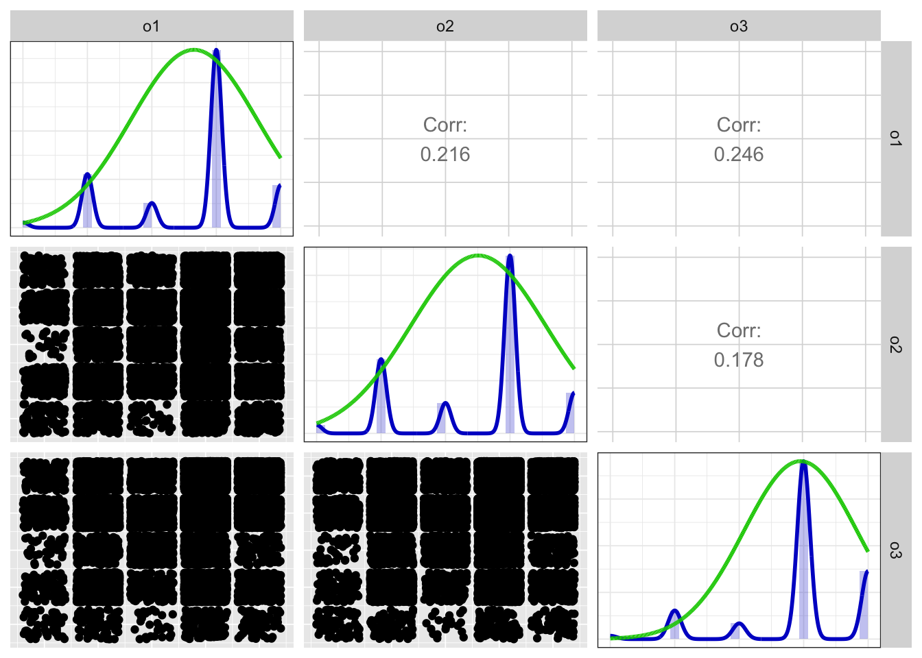

x$scatterMatrix$output$scatterMatrix <- no_md()

Detailed output

print(x)

## 
## Information about this analysis:
## 
##                  Dataframe: res$dat
##                      Items: o1, o2, o3
##               Observations: 31446
##      Positive correlations: 3 out of 3 (100%)
## 
## Estimates assuming interval level:
## 
##              Omega (total): 0.45
##       Omega (hierarchical): 0.43
##    Revelle's omega (total): 0.46
## Greatest Lower Bound (GLB): 0.46
##              Coefficient H: 0.46
##           Cronbach's alpha: 0.45
## Confidence intervals:
##              Omega (total): [0.44, 0.46]
##           Cronbach's alpha: [0.43, 0.46]
## 
## Estimates assuming ordinal level:
## 
##      Ordinal Omega (total): 0.53
##  Ordinal Omega (hierarch.): 0.53
##   Ordinal Cronbach's alpha: 0.52
## Confidence intervals:
##      Ordinal Omega (total): [0.52, 0.54]
##   Ordinal Cronbach's alpha: [0.51, 0.53]
## 
## Note: the normal point estimate and confidence interval for omega are based on the procedure suggested by Dunn, Baguley & Brunsden (2013) using the MBESS function ci.reliability, whereas the psych package point estimate was suggested in Revelle & Zinbarg (2008). See the help ('?scaleStructure') for more information.
## 
## Eigen values: 1.428, 0.826, 0.747
## Loadings:
##    PC1  
## o1 0.726
## o2 0.653
## o3 0.689
## 
##                  PC1
## SS loadings    1.428
## Proportion Var 0.476
## 
##    vars     n mean   sd median trimmed mad min max range  skew kurtosis   se
## o1    1 31446 3.65 0.98      4    3.71   0   1   5     4 -0.83    -0.13 0.01
## o2    2 31446 3.51 1.05      4    3.54   0   1   5     4 -0.62    -0.66 0.01
## o3    3 31446 3.95 0.88      4    4.08   0   1   5     4 -1.16     1.32 0.00

Summary statistics

for (i in seq_along(names(items))) {
  attributes(items[[i]]) = recursive_escape(attributes(items[[i]]))
}
escaped_table(codebook_table(items))

## 
## 
## name   label                                     data_type        value_labels                                                                                                                   n_missing   complete_rate  min   median   max     mean       sd   n_value_labels  hist     
## -----  ----------------------------------------  ---------------  ----------------------------------------------------------------------------------------------------------------------------  ----------  --------------  ----  -------  ----  ------  -------  ---------------  ---------
## o1     Is original, comes up with new ideas.     haven_labelled   1. Disagree strongly,<br>2. Disagree a little,<br>3. Neither agree nor disagree,<br>4. Agree a little,<br>5. Agree strongly        69795          0.3106  1     4        5      3.654   0.9819                5  ▁▂▁▁▁▇▁▂ 
## o2     Has an active imagination.                haven_labelled   1. Disagree strongly,<br>2. Disagree a little,<br>3. Neither agree nor disagree,<br>4. Agree a little,<br>5. Agree strongly        69795          0.3106  1     4        5      3.508   1.0456                5  ▁▃▁▂▁▇▁▂ 
## o3     Values artistic, aesthetic experiences.   haven_labelled   1. Disagree strongly,<br>2. Disagree a little,<br>3. Neither agree nor disagree,<br>4. Agree a little,<br>5. Agree strongly        69795          0.3106  1     4        5      3.950   0.8793                5  ▁▁▁▁▁▇▁▃

Scale: big5_neu

Overview

Reliability: Not computed.

Missing: 69795.

old_height <- knitr::opts_chunk$get("fig.height")
new_height <- length(scale_info$scale_item_names)
new_height <- ifelse(new_height > 20, 20, new_height)
new_height <- ifelse(new_height < 1, 1, new_height)
new_height <- ifelse(is.na(new_height) | is.nan(new_height), 
                     old_height, new_height)
knitr::opts_chunk$set(fig.height = new_height)

if (dplyr::n_distinct(na.omit(unlist(items))) < 12) {
  likert_plot <- likert_from_items(items)
  if (!is.null(likert_plot)) {
    graphics::plot(likert_plot)
  }
}

knitr::opts_chunk$set(fig.height = old_height)

wrap_at <- knitr::opts_chunk$get("fig.width") * 10

dist_plot <- plot_labelled(scale, scale_name, wrap_at)

choices <- attributes(items[[1]])$item$choices
breaks <- as.numeric(names(choices))
if (length(breaks)) {
  suppressMessages( # ignore message about overwriting x axis
  dist_plot <- dist_plot +
        ggplot2::scale_x_continuous("values", 
                                breaks = breaks, 
                                labels = stringr::str_wrap(unlist(choices), ceiling(wrap_at * 0.21))) +
      ggplot2::expand_limits(x = range(breaks)))
  
}

dist_plot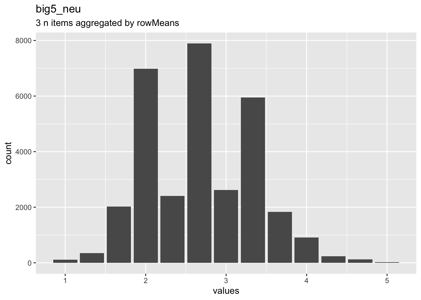

Reliability details

for (i in seq_along(reliabilities)) {
  rel <- reliabilities[[i]]
  cat(knitr::knit_print(rel, indent = paste0(indent, "####")))
}

Summary statistics

for (i in seq_along(names(items))) {
  attributes(items[[i]]) = recursive_escape(attributes(items[[i]]))
}
escaped_table(codebook_table(items))

## 
## 
## name           label                  data_type        value_labels                                                                                                                   n_missing   complete_rate  min   median   max     mean       sd   n_value_labels  hist     
## -------------  ---------------------  ---------------  ----------------------------------------------------------------------------------------------------------------------------  ----------  --------------  ----  -------  ----  ------  -------  ---------------  ---------
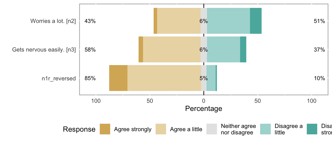
## n1r_reversed   NA                     haven_labelled   5. Disagree strongly,<br>4. Disagree a little,<br>3. Neither agree nor disagree,<br>2. Agree a little,<br>1. Agree strongly        69795          0.3106  1     2        5      2.087   0.8107                5  ▂▇▁▁▁▁▁▁ 
## n2             Worries a lot.         haven_labelled   1. Disagree strongly,<br>2. Disagree a little,<br>3. Neither agree nor disagree,<br>4. Agree a little,<br>5. Agree strongly        69795          0.3106  1     4        5      3.148   1.1541                5  ▁▇▁▁▁▇▁▂ 
## n3             Gets nervous easily.   haven_labelled   1. Disagree strongly,<br>2. Disagree a little,<br>3. Neither agree nor disagree,<br>4. Agree a little,<br>5. Agree strongly        69795          0.3106  1     2        5      2.806   1.0969                5  ▁▇▁▁▁▅▁▁

Scale: big5_agree

Overview

Reliability: ω_ordinal [95% CI] = 0.57 [0.55;0.59].

Missing: 69795.

old_height <- knitr::opts_chunk$get("fig.height")
new_height <- length(scale_info$scale_item_names)
new_height <- ifelse(new_height > 20, 20, new_height)
new_height <- ifelse(new_height < 1, 1, new_height)
new_height <- ifelse(is.na(new_height) | is.nan(new_height), 
                     old_height, new_height)
knitr::opts_chunk$set(fig.height = new_height)

if (dplyr::n_distinct(na.omit(unlist(items))) < 12) {
  likert_plot <- likert_from_items(items)
  if (!is.null(likert_plot)) {
    graphics::plot(likert_plot)
  }
}

knitr::opts_chunk$set(fig.height = old_height)

wrap_at <- knitr::opts_chunk$get("fig.width") * 10

dist_plot <- plot_labelled(scale, scale_name, wrap_at)

choices <- attributes(items[[1]])$item$choices
breaks <- as.numeric(names(choices))
if (length(breaks)) {
  suppressMessages( # ignore message about overwriting x axis
  dist_plot <- dist_plot +
        ggplot2::scale_x_continuous("values", 
                                breaks = breaks, 
                                labels = stringr::str_wrap(unlist(choices), ceiling(wrap_at * 0.21))) +
      ggplot2::expand_limits(x = range(breaks)))
  
}

dist_plot

Reliability details

for (i in seq_along(reliabilities)) {
  rel <- reliabilities[[i]]
  cat(knitr::knit_print(rel, indent = paste0(indent, "####")))
}

Reliability Indices

coefs <- x$scaleReliability$output$dat %>% 
  tidyr::gather(index, estimate) %>% 
  dplyr::filter(index != "n.items", index != "n.observations") %>% 
  dplyr::mutate(index = stringr::str_to_title(
    stringr::str_replace_all(index,
      stringr::fixed("."), " ")))

cis <- coefs %>% 
  dplyr::filter(stringr::str_detect(index, " Ci ")) %>% 
  tidyr::separate(index, c("index", "hilo"), sep = " Ci ") %>% 
  tidyr::spread(hilo, estimate)
if (nrow(cis)) {
  cis <- cis %>% dplyr::rename(
    `Lower 95% CI` = .data$Lo, `Upper 95% CI` = .data$Hi
  )
}

coefs_with_cis <- coefs %>% 
  dplyr::filter(!stringr::str_detect(index, " Ci ")) %>% 
    dplyr::left_join(cis, by = "index") %>% 
    dplyr::mutate(index = dplyr::if_else(index == "Glb", "Greatest Lower Bound", .data$index)) %>% 
    dplyr::arrange(!stringr::str_detect(index, "Omega")) %>% 
    dplyr::select(Index = .data$index, Estimate = .data$estimate)


pander::pander(coefs_with_cis)

Index	Estimate
Omega	0.3774
Omega Psych Tot	0.444
Omega Psych H	0.01546
Omega Ordinal	0.5685
Cronbach Alpha	0.2718
Greatest Lower Bound	0.4653
Alpha Ordinal	0.4498

Positive correlations: 3 out of 3 (100%)

Scatter matrix

print(x$scatterMatrix$output$scatterMatrix)

x$scatterMatrix$output$scatterMatrix <- no_md()

Detailed output

print(x)

## 
## Information about this analysis:
## 
##                  Dataframe: res$dat
##                      Items: a1, a2, a3r_reversed
##               Observations: 31446
##      Positive correlations: 3 out of 3 (100%)
## 
## Estimates assuming interval level:
## 
##              Omega (total): 0.38
##       Omega (hierarchical): 0.02
##    Revelle's omega (total): 0.44
## Greatest Lower Bound (GLB): 0.47
##              Coefficient H: 0.86
##           Cronbach's alpha: 0.27
## Confidence intervals:
##              Omega (total): [0.31, 0.44]
##           Cronbach's alpha: [0.26, 0.28]
## 
## Estimates assuming ordinal level:
## 
##      Ordinal Omega (total): 0.57
##  Ordinal Omega (hierarch.): 0.57
##   Ordinal Cronbach's alpha: 0.45
## Confidence intervals:
##      Ordinal Omega (total): [0.55, 0.59]
##   Ordinal Cronbach's alpha: [0.44, 0.46]
## 
## Note: the normal point estimate and confidence interval for omega are based on the procedure suggested by Dunn, Baguley & Brunsden (2013) using the MBESS function ci.reliability, whereas the psych package point estimate was suggested in Revelle & Zinbarg (2008). See the help ('?scaleStructure') for more information.
## 
## Eigen values: 1.396, 0.996, 0.608
## Loadings:
##              PC1  
## a1           0.832
## a2           0.829
## a3r_reversed 0.127
## 
##                  PC1
## SS loadings    1.396
## Proportion Var 0.465
## 
##              vars     n mean   sd median trimmed mad min max range  skew kurtosis   se
## a1              1 31446 4.17 0.67      4    4.23   0   1   5     4 -1.16     3.54 0.00
## a2              2 31446 4.12 0.66      4    4.18   0   1   5     4 -1.11     3.60 0.00
## a3r_reversed    3 31446 3.41 1.02      4    3.47   0   1   5     4 -0.71    -0.68 0.01

Summary statistics

for (i in seq_along(names(items))) {
  attributes(items[[i]]) = recursive_escape(attributes(items[[i]]))
}
escaped_table(codebook_table(items))

## 
## 
## name           label                                         data_type        value_labels                                                                                                                   n_missing   complete_rate  min   median   max     mean       sd   n_value_labels  hist     
## -------------  --------------------------------------------  ---------------  ----------------------------------------------------------------------------------------------------------------------------  ----------  --------------  ----  -------  ----  ------  -------  ---------------  ---------
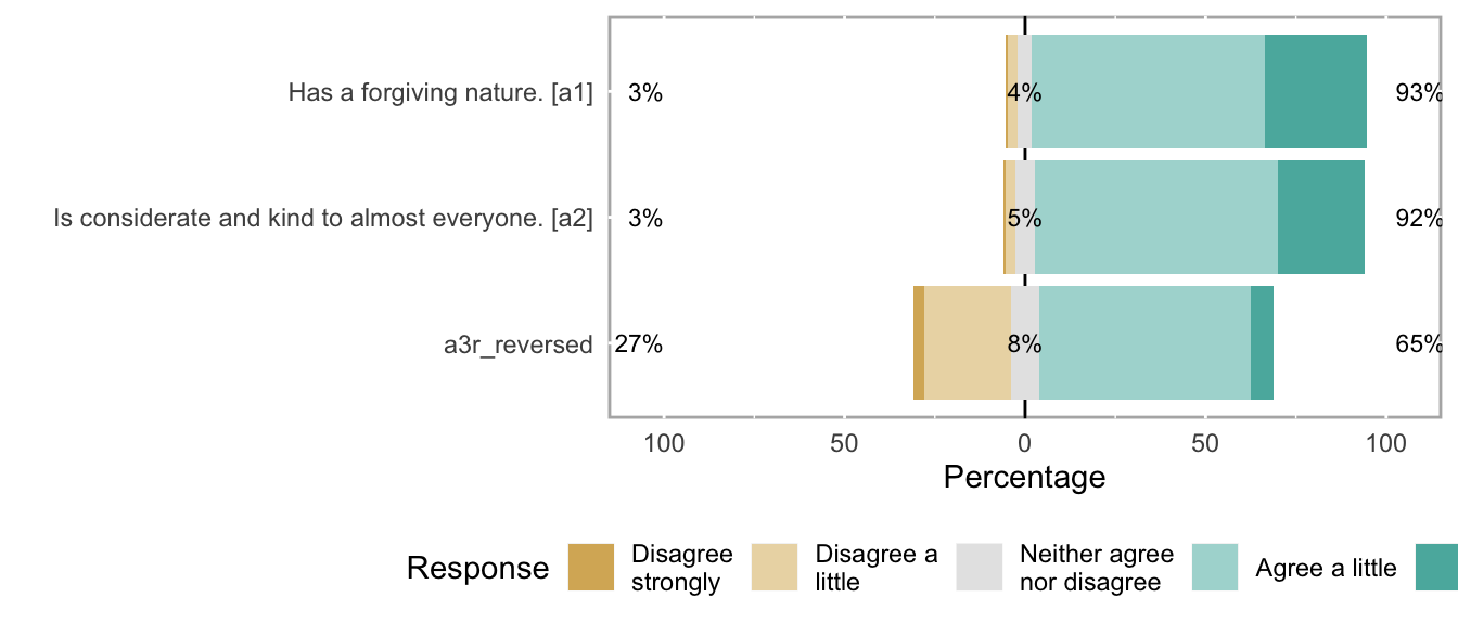
## a1             Has a forgiving nature.                       haven_labelled   1. Disagree strongly,<br>2. Disagree a little,<br>3. Neither agree nor disagree,<br>4. Agree a little,<br>5. Agree strongly        69795          0.3106  1     4        5      4.175   0.6696                5  ▁▁▁▁▁▇▁▃ 
## a2             Is considerate and kind to almost everyone.   haven_labelled   1. Disagree strongly,<br>2. Disagree a little,<br>3. Neither agree nor disagree,<br>4. Agree a little,<br>5. Agree strongly        69795          0.3106  1     4        5      4.119   0.6567                5  ▁▁▁▁▁▇▁▃ 
## a3r_reversed   NA                                            haven_labelled   5. Disagree strongly,<br>4. Disagree a little,<br>3. Neither agree nor disagree,<br>2. Agree a little,<br>1. Agree strongly        69795          0.3106  1     4        5      3.412   1.0235                5  ▁▃▁▁▁▇▁▁

missingness_report

items

Codebook table

export_table(metadata_table)

jsonld

JSON-LD metadata

The following JSON-LD can be found by search engines, if you share this codebook publicly on the web.

{
  "name": "Indonesian Family Life Study, merged subset",
  "description": "Data from the IFLS, merged across waves, most outcomes taken from wave 5. Includes birth order, family structure, Big 5 Personality, intelligence tests, and risk lotteries\n\n\n## Table of variables\nThis table contains variable names, labels, and number of missing values.\nSee the complete codebook for more.\n\n[truncated]\n\n### Note\nThis dataset was automatically described using the [codebook R package](https://rubenarslan.github.io/codebook/) (version 0.8.2).",
  "identifier": "https://www.rand.org/well-being/social-and-behavioral-policy/data/FLS/IFLS.html",
  "creator": "RAND corporation",
  "citation": "Strauss, J., Witoelar, F., & Sikoki, B. (2016). The Fifth Wave of the Indonesia Family Life Survey: Overview and Field Report. WR-1143/1-NIA/NICHD",
  "url": "https://www.rand.org/well-being/social-and-behavioral-policy/data/FLS/IFLS.html",
  "datePublished": "2016",
  "temporalCoverage": "2014/2015",
  "spatialCoverage": "13 Indonesian provinces. The sample is representative of about 83% of the Indonesian population and contains over 30,000 individuals living in 13 of the 27 provinces in the country. See URL for more.",
  "keywords": ["wave", "mother_pidlink", "chron_order_birth", "lifebirths", "multiple_birth", "alive", "birthdate", "any_multiple_birth", "marriage_id", "birthorder_uterus_preg", "sibling_count_uterus_preg", "birthorder_uterus_alive", "sibling_count_uterus_alive", "birthorder_genes", "sibling_count_genes", "pidlink", "father_pidlink", "age", "death_yr", "death_month", "sc05", "province", "sc01_14_14", "sibling_count_naive_ind", "any_multiple_birthdate", "birthorder_naive", "sibling_count_naive", "age_2015_old", "age_2015_young", "raven_2015_young", "math_2015_young", "raven_2015_old", "math_2015_old", "words_immediate", "words_delayed", "words_remembered_avg", "adaptive_numbering", "age_2007_young", "age_2007_old", "raven_2007_old", "raven_2007_young", "math_2007_young", "math_2007_old", "count_backwards", "g_factor_2015_old", "g_factor_2015_young", "g_factor_2007_old", "g_factor_2007_young", "e1", "c1", "o1", "e2r", "n1r", "a1", "n2", "o2", "c2r", "o3", "a2", "c3", "e3", "a3r", "n3", "e2r_reversed", "big5_ext", "c2r_reversed", "big5_con", "big5_open", "n1r_reversed", "big5_neu", "a3r_reversed", "big5_agree", "random_si", "si01", "si02", "si03", "si04", "si05", "si11", "si12", "si13", "si14", "si15", "riskA", "riskB", "attended_school", "highest_education", "currently_attending_school", "hours_in_class", "years_of_education", "Type_of_test_elementary", "Indonesia_score_elementary", "English_score_elementary", "Math_score_elemenatry", "Total_score_elemenatry", "Type_of_test_Junior_High", "Indonesia_score_Junior_High", "English_score_Junior_High", "Math_score_Junior_High", "Total_score_Junior_High", "Type_of_test_Senior_High", "Indonesia_score_Senior_High", "English_score_Senior_High", "Math_score_Senior_High", "Total_score_Senior_High", "Total_score_highest", "Total_score_highest_type", "Math_score_highest", "Math_score_highest_type", "Elementary_worked", "Junior_high_worked", "Senior_high_worked", "University_worked", "total_worked", "Elementary_missed", "Junior_high_missed", "Senior_high_missed", "University_missed", "total_missed", "Category", "Sector", "Self_employed", "ever_smoked", "still_smoking", "amount", "age_first_smoke", "amount_still_smokers", "male", "wage_last_month_log", "wage_last_year_log", "money_spent_smoking_log", "birthyear", "birthorder_naive_factor", "sibling_count_naive_factor", "birthorder_uterus_alive_factor", "sibling_count_uterus_alive_factor", "birthorder_uterus_preg_factor", "sibling_count_uterus_preg_factor", "birthorder_genes_factor", "sibling_count_genes_factor", "count_birthorder_naive", "count_birthorder_uterus_alive", "count_birthorder_uterus_preg", "count_birthorder_genes", "sibling_count", "birth_order_nonlinear", "birth_order", "count_birth_order"],
  "@context": "http://schema.org/",
  "@type": "Dataset",
  "variableMeasured": [
    {
      "name": "wave",
      "@type": "propertyValue"
    },
    {
      "name": "mother_pidlink",
      "@type": "propertyValue"
    },
    {
      "name": "chron_order_birth",
      "description": "Chronological order of pregnancy's outcome",
      "@type": "propertyValue"
    },
    {
      "name": "lifebirths",
      "value": "1. 2,\n2. 3,\n3. 4",
      "@type": "propertyValue"
    },
    {
      "name": "multiple_birth",
      "@type": "propertyValue"
    },
    {
      "name": "alive",
      "@type": "propertyValue"
    },
    {
      "name": "birthdate",
      "@type": "propertyValue"
    },
    {
      "name": "any_multiple_birth",
      "@type": "propertyValue"
    },
    {
      "name": "marriage_id",
      "@type": "propertyValue"
    },
    {
      "name": "birthorder_uterus_preg",
      "@type": "propertyValue"
    },
    {
      "name": "sibling_count_uterus_preg",
      "@type": "propertyValue"
    },
    {
      "name": "birthorder_uterus_alive",
      "@type": "propertyValue"
    },
    {
      "name": "sibling_count_uterus_alive",
      "@type": "propertyValue"
    },
    {
      "name": "birthorder_genes",
      "@type": "propertyValue"
    },
    {
      "name": "sibling_count_genes",
      "@type": "propertyValue"
    },
    {
      "name": "pidlink",
      "@type": "propertyValue"
    },
    {
      "name": "father_pidlink",
      "@type": "propertyValue"
    },
    {
      "name": "age",
      "description": "Age now",
      "@type": "propertyValue"
    },
    {
      "name": "death_yr",
      "@type": "propertyValue"
    },
    {
      "name": "death_month",
      "description": "Departure/entry into HH (Month)",
      "@type": "propertyValue"
    },
    {
      "name": "sc05",
      "description": "Urban/Rural",
      "value": "1. 1:Urban,\n2. 2:Rural",
      "maxValue": 2,
      "minValue": 1,
      "@type": "propertyValue"
    },
    {
      "name": "province",
      "@type": "propertyValue"
    },
    {
      "name": "sc01_14_14",
      "description": "2014 Province, 2014 BPS Code",
      "@type": "propertyValue"
    },
    {
      "name": "sibling_count_naive_ind",
      "@type": "propertyValue"
    },
    {
      "name": "any_multiple_birthdate",
      "@type": "propertyValue"
    },
    {
      "name": "birthorder_naive",
      "@type": "propertyValue"
    },
    {
      "name": "sibling_count_naive",
      "@type": "propertyValue"
    },
    {
      "name": "age_2015_old",
      "@type": "propertyValue"
    },
    {
      "name": "age_2015_young",
      "@type": "propertyValue"
    },
    {
      "name": "raven_2015_young",
      "@type": "propertyValue"
    },
    {
      "name": "math_2015_young",
      "@type": "propertyValue"
    },
    {
      "name": "raven_2015_old",
      "@type": "propertyValue"
    },
    {
      "name": "math_2015_old",
      "@type": "propertyValue"
    },
    {
      "name": "words_immediate",
      "description": "count of immediate recall words",
      "@type": "propertyValue"
    },
    {
      "name": "words_delayed",
      "description": "count of delayed recall words",
      "@type": "propertyValue"
    },
    {
      "name": "words_remembered_avg",
      "@type": "propertyValue"
    },
    {
      "name": "adaptive_numbering",
      "description": "W-score",
      "@type": "propertyValue"
    },
    {
      "name": "age_2007_young",
      "@type": "propertyValue"
    },
    {
      "name": "age_2007_old",
      "@type": "propertyValue"
    },
    {
      "name": "raven_2007_old",
      "@type": "propertyValue"
    },
    {
      "name": "raven_2007_young",
      "@type": "propertyValue"
    },
    {
      "name": "math_2007_young",
      "@type": "propertyValue"
    },
    {
      "name": "math_2007_old",
      "@type": "propertyValue"
    },
    {
      "name": "count_backwards",
      "@type": "propertyValue"
    },
    {
      "name": "g_factor_2015_old",
      "@type": "propertyValue"
    },
    {
      "name": "g_factor_2015_young",
      "@type": "propertyValue"
    },
    {
      "name": "g_factor_2007_old",
      "@type": "propertyValue"
    },
    {
      "name": "g_factor_2007_young",
      "@type": "propertyValue"
    },
    {
      "name": "e1",
      "description": "Is talkative",
      "value": "1. Disagree strongly,\n2. Disagree a little,\n3. Neither agree nor disagree,\n4. Agree a little,\n5. Agree strongly",
      "maxValue": 5,
      "minValue": 1,
      "@type": "propertyValue"
    },
    {
      "name": "c1",
      "description": "Does a thorough job",
      "value": "1. Disagree strongly,\n2. Disagree a little,\n3. Neither agree nor disagree,\n4. Agree a little,\n5. Agree strongly",
      "maxValue": 5,
      "minValue": 1,
      "@type": "propertyValue"
    },
    {
      "name": "o1",
      "description": "Is original, comes up with new ideas.",
      "value": "1. Disagree strongly,\n2. Disagree a little,\n3. Neither agree nor disagree,\n4. Agree a little,\n5. Agree strongly",
      "maxValue": 5,
      "minValue": 1,
      "@type": "propertyValue"
    },
    {
      "name": "e2r",
      "value": "1. Disagree strongly,\n2. Disagree a little,\n3. Neither agree nor disagree,\n4. Agree a little,\n5. Agree strongly",
      "maxValue": 5,
      "minValue": 1,
      "@type": "propertyValue"
    },
    {
      "name": "n1r",
      "value": "1. Disagree strongly,\n2. Disagree a little,\n3. Neither agree nor disagree,\n4. Agree a little,\n5. Agree strongly",
      "maxValue": 5,
      "minValue": 1,
      "@type": "propertyValue"
    },
    {
      "name": "a1",
      "description": "Has a forgiving nature.",
      "value": "1. Disagree strongly,\n2. Disagree a little,\n3. Neither agree nor disagree,\n4. Agree a little,\n5. Agree strongly",
      "maxValue": 5,
      "minValue": 1,
      "@type": "propertyValue"
    },
    {
      "name": "n2",
      "description": "Worries a lot.",
      "value": "1. Disagree strongly,\n2. Disagree a little,\n3. Neither agree nor disagree,\n4. Agree a little,\n5. Agree strongly",
      "maxValue": 5,
      "minValue": 1,
      "@type": "propertyValue"
    },
    {
      "name": "o2",
      "description": "Has an active imagination.",
      "value": "1. Disagree strongly,\n2. Disagree a little,\n3. Neither agree nor disagree,\n4. Agree a little,\n5. Agree strongly",
      "maxValue": 5,
      "minValue": 1,
      "@type": "propertyValue"
    },
    {
      "name": "c2r",
      "value": "1. Disagree strongly,\n2. Disagree a little,\n3. Neither agree nor disagree,\n4. Agree a little,\n5. Agree strongly",
      "maxValue": 5,
      "minValue": 1,
      "@type": "propertyValue"
    },
    {
      "name": "o3",
      "description": "Values artistic, aesthetic experiences.",
      "value": "1. Disagree strongly,\n2. Disagree a little,\n3. Neither agree nor disagree,\n4. Agree a little,\n5. Agree strongly",
      "maxValue": 5,
      "minValue": 1,
      "@type": "propertyValue"
    },
    {
      "name": "a2",
      "description": "Is considerate and kind to almost everyone.",
      "value": "1. Disagree strongly,\n2. Disagree a little,\n3. Neither agree nor disagree,\n4. Agree a little,\n5. Agree strongly",
      "maxValue": 5,
      "minValue": 1,
      "@type": "propertyValue"
    },
    {
      "name": "c3",
      "description": "Does things efficiently.",
      "value": "1. Disagree strongly,\n2. Disagree a little,\n3. Neither agree nor disagree,\n4. Agree a little,\n5. Agree strongly",
      "maxValue": 5,
      "minValue": 1,
      "@type": "propertyValue"
    },
    {
      "name": "e3",
      "description": "Outgoing, sociable.",
      "value": "1. Disagree strongly,\n2. Disagree a little,\n3. Neither agree nor disagree,\n4. Agree a little,\n5. Agree strongly",
      "maxValue": 5,
      "minValue": 1,
      "@type": "propertyValue"
    },
    {
      "name": "a3r",
      "value": "1. Disagree strongly,\n2. Disagree a little,\n3. Neither agree nor disagree,\n4. Agree a little,\n5. Agree strongly",
      "maxValue": 5,
      "minValue": 1,
      "@type": "propertyValue"
    },
    {
      "name": "n3",
      "description": "Gets nervous easily.",
      "value": "1. Disagree strongly,\n2. Disagree a little,\n3. Neither agree nor disagree,\n4. Agree a little,\n5. Agree strongly",
      "maxValue": 5,
      "minValue": 1,
      "@type": "propertyValue"
    },
    {
      "name": "e2r_reversed",
      "value": "5. Disagree strongly,\n4. Disagree a little,\n3. Neither agree nor disagree,\n2. Agree a little,\n1. Agree strongly",
      "maxValue": 5,
      "minValue": 1,
      "@type": "propertyValue"
    },
    {
      "name": "big5_ext",
      "description": "3 e items aggregated by rowMeans",
      "@type": "propertyValue"
    },
    {
      "name": "c2r_reversed",
      "value": "5. Disagree strongly,\n4. Disagree a little,\n3. Neither agree nor disagree,\n2. Agree a little,\n1. Agree strongly",
      "maxValue": 5,
      "minValue": 1,
      "@type": "propertyValue"
    },
    {
      "name": "big5_con",
      "description": "3 c items aggregated by rowMeans",
      "@type": "propertyValue"
    },
    {
      "name": "big5_open",
      "description": "3 o items aggregated by rowMeans",
      "@type": "propertyValue"
    },
    {
      "name": "n1r_reversed",
      "value": "5. Disagree strongly,\n4. Disagree a little,\n3. Neither agree nor disagree,\n2. Agree a little,\n1. Agree strongly",
      "maxValue": 5,
      "minValue": 1,
      "@type": "propertyValue"
    },
    {
      "name": "big5_neu",
      "description": "3 n items aggregated by rowMeans",
      "@type": "propertyValue"
    },
    {
      "name": "a3r_reversed",
      "value": "5. Disagree strongly,\n4. Disagree a little,\n3. Neither agree nor disagree,\n2. Agree a little,\n1. Agree strongly",
      "maxValue": 5,
      "minValue": 1,
      "@type": "propertyValue"
    },
    {
      "name": "big5_agree",
      "description": "3 a items aggregated by rowMeans",
      "@type": "propertyValue"
    },
    {
      "name": "random_si",
      "value": "1. 1,\n2. 2",
      "@type": "propertyValue"
    },
    {
      "name": "si01",
      "@type": "propertyValue"
    },
    {
      "name": "si02",
      "@type": "propertyValue"
    },
    {
      "name": "si03",
      "@type": "propertyValue"
    },
    {
      "name": "si04",
      "@type": "propertyValue"
    },
    {
      "name": "si05",
      "@type": "propertyValue"
    },
    {
      "name": "si11",
      "@type": "propertyValue"
    },
    {
      "name": "si12",
      "@type": "propertyValue"
    },
    {
      "name": "si13",
      "@type": "propertyValue"
    },
    {
      "name": "si14",
      "@type": "propertyValue"
    },
    {
      "name": "si15",
      "@type": "propertyValue"
    },
    {
      "name": "riskA",
      "@type": "propertyValue"
    },
    {
      "name": "riskB",
      "@type": "propertyValue"
    },
    {
      "name": "attended_school",
      "@type": "propertyValue"
    },
    {
      "name": "highest_education",
      "value": "1. Elementary,\n2. Junior High,\n3. Senior High,\n4. University",
      "@type": "propertyValue"
    },
    {
      "name": "currently_attending_school",
      "value": "1. no,\n2. yes",
      "@type": "propertyValue"
    },
    {
      "name": "hours_in_class",
      "@type": "propertyValue"
    },
    {
      "name": "years_of_education",
      "@type": "propertyValue"
    },
    {
      "name": "Type_of_test_elementary",
      "value": "1. EBTANAS,\n2. UAN/UN",
      "@type": "propertyValue"
    },
    {
      "name": "Indonesia_score_elementary",
      "@type": "propertyValue"
    },
    {
      "name": "English_score_elementary",
      "@type": "propertyValue"
    },
    {
      "name": "Math_score_elemenatry",
      "@type": "propertyValue"
    },
    {
      "name": "Total_score_elemenatry",
      "description": "Total EBTANAS/UAN/UN score",
      "@type": "propertyValue"
    },
    {
      "name": "Type_of_test_Junior_High",
      "value": "1. EBTANAS,\n2. UAN/UN",
      "@type": "propertyValue"
    },
    {
      "name": "Indonesia_score_Junior_High",
      "@type": "propertyValue"
    },
    {
      "name": "English_score_Junior_High",
      "@type": "propertyValue"
    },
    {
      "name": "Math_score_Junior_High",
      "@type": "propertyValue"
    },
    {
      "name": "Total_score_Junior_High",
      "description": "Total EBTANAS/UAN/UN score",
      "@type": "propertyValue"
    },
    {
      "name": "Type_of_test_Senior_High",
      "value": "1. EBTANAS,\n2. UAN/UN",
      "@type": "propertyValue"
    },
    {
      "name": "Indonesia_score_Senior_High",
      "@type": "propertyValue"
    },
    {
      "name": "English_score_Senior_High",
      "@type": "propertyValue"
    },
    {
      "name": "Math_score_Senior_High",
      "@type": "propertyValue"
    },
    {
      "name": "Total_score_Senior_High",
      "description": "Total EBTANAS/UAN/UN score",
      "@type": "propertyValue"
    },
    {
      "name": "Total_score_highest",
      "@type": "propertyValue"
    },
    {
      "name": "Total_score_highest_type",
      "value": "1. Elementary,\n2. Junior High,\n3. Senior High",
      "@type": "propertyValue"
    },
    {
      "name": "Math_score_highest",
      "@type": "propertyValue"
    },
    {
      "name": "Math_score_highest_type",
      "value": "1. Elementary,\n2. Junior High,\n3. Senior High",
      "@type": "propertyValue"
    },
    {
      "name": "Elementary_worked",
      "@type": "propertyValue"
    },
    {
      "name": "Junior_high_worked",
      "@type": "propertyValue"
    },
    {
      "name": "Senior_high_worked",
      "@type": "propertyValue"
    },
    {
      "name": "University_worked",
      "@type": "propertyValue"
    },
    {
      "name": "total_worked",
      "@type": "propertyValue"
    },
    {
      "name": "Elementary_missed",
      "@type": "propertyValue"
    },
    {
      "name": "Junior_high_missed",
      "@type": "propertyValue"
    },
    {
      "name": "Senior_high_missed",
      "@type": "propertyValue"
    },
    {
      "name": "University_missed",
      "@type": "propertyValue"
    },
    {
      "name": "total_missed",
      "@type": "propertyValue"
    },
    {
      "name": "Category",
      "value": "1. Casual worker in agriculture,\n2. Casual worker not in agriculture,\n3. Government worker,\n4. Private worker,\n5. Self-employed,\n6. Unpaid family worker",
      "@type": "propertyValue"
    },
    {
      "name": "Sector",
      "value": "1. Agriculture, forestry, fishing and hunting,\n2. Construction,\n3. Electricity, gas, water,\n4. Finance, insurance, real estate and business services,\n5. Manufacturing,\n6. Mining and quarrying,\n7. Social services,\n8. Transportation, storage and communications,\n9. Wholesale, retail, restaurants and hotels",
      "@type": "propertyValue"
    },
    {
      "name": "Self_employed",
      "@type": "propertyValue"
    },
    {
      "name": "ever_smoked",
      "@type": "propertyValue"
    },
    {
      "name": "still_smoking",
      "@type": "propertyValue"
    },
    {
      "name": "amount",
      "@type": "propertyValue"
    },
    {
      "name": "age_first_smoke",
      "description": "At what age did you start to smoke on a regular basis?",
      "@type": "propertyValue"
    },
    {
      "name": "amount_still_smokers",
      "@type": "propertyValue"
    },
    {
      "name": "male",
      "@type": "propertyValue"
    },
    {
      "name": "wage_last_month_log",
      "@type": "propertyValue"
    },
    {
      "name": "wage_last_year_log",
      "@type": "propertyValue"
    },
    {
      "name": "money_spent_smoking_log",
      "@type": "propertyValue"
    },
    {
      "name": "birthyear",
      "@type": "propertyValue"
    },
    {
      "name": "birthorder_naive_factor",
      "value": "1. 1,\n2. 2,\n3. 3,\n4. 4,\n5. 5,\n6. >5",
      "@type": "propertyValue"
    },
    {
      "name": "sibling_count_naive_factor",
      "value": "1. 2,\n2. 3,\n3. 4,\n4. 5,\n5. >5",
      "@type": "propertyValue"
    },
    {
      "name": "birthorder_uterus_alive_factor",
      "value": "1. 1,\n2. 2,\n3. 3,\n4. 4,\n5. 5,\n6. >5",
      "@type": "propertyValue"
    },
    {
      "name": "sibling_count_uterus_alive_factor",
      "value": "1. 2,\n2. 3,\n3. 4,\n4. 5,\n5. >5",
      "@type": "propertyValue"
    },
    {
      "name": "birthorder_uterus_preg_factor",
      "value": "1. 1,\n2. 2,\n3. 3,\n4. 4,\n5. 5,\n6. >5",
      "@type": "propertyValue"
    },
    {
      "name": "sibling_count_uterus_preg_factor",
      "value": "1. 2,\n2. 3,\n3. 4,\n4. 5,\n5. >5",
      "@type": "propertyValue"
    },
    {
      "name": "birthorder_genes_factor",
      "value": "1. 1,\n2. 2,\n3. 3,\n4. 4,\n5. 5,\n6. >5",
      "@type": "propertyValue"
    },
    {
      "name": "sibling_count_genes_factor",
      "value": "1. 2,\n2. 3,\n3. 4,\n4. 5,\n5. >5",
      "@type": "propertyValue"
    },
    {
      "name": "count_birthorder_naive",
      "value": "1. 1/2,\n2. 2/2,\n3. 1/3,\n4. 2/3,\n5. 3/3,\n6. 1/4,\n7. 2/4,\n8. 3/4,\n9. 4/4,\n10. 1/5,\n11. 2/5,\n12. 3/5,\n13. 4/5,\n14. 5/5,\n15. 1/>5,\n16. 2/>5,\n17. 3/>5,\n18. 4/>5,\n19. 5/>5,\n20. >5/>5",
      "@type": "propertyValue"
    },
    {
      "name": "count_birthorder_uterus_alive",
      "value": "1. 1/2,\n2. 2/2,\n3. 1/3,\n4. 2/3,\n5. 3/3,\n6. 1/4,\n7. 2/4,\n8. 3/4,\n9. 4/4,\n10. 1/5,\n11. 2/5,\n12. 3/5,\n13. 4/5,\n14. 5/5,\n15. 1/>5,\n16. 2/>5,\n17. 3/>5,\n18. 4/>5,\n19. 5/>5,\n20. >5/>5",
      "@type": "propertyValue"
    },
    {
      "name": "count_birthorder_uterus_preg",
      "value": "1. 1/2,\n2. 2/2,\n3. 1/3,\n4. 2/3,\n5. 3/3,\n6. 1/4,\n7. 2/4,\n8. 3/4,\n9. 4/4,\n10. 1/5,\n11. 2/5,\n12. 3/5,\n13. 4/5,\n14. 5/5,\n15. 1/>5,\n16. 2/>5,\n17. 3/>5,\n18. 4/>5,\n19. 5/>5,\n20. >5/>5",
      "@type": "propertyValue"
    },
    {
      "name": "count_birthorder_genes",
      "value": "1. 1/2,\n2. 2/2,\n3. 1/3,\n4. 2/3,\n5. 3/3,\n6. 1/4,\n7. 2/4,\n8. 3/4,\n9. 4/4,\n10. 1/5,\n11. 2/5,\n12. 3/5,\n13. 4/5,\n14. 5/5,\n15. 1/>5,\n16. 2/>5,\n17. 3/>5,\n18. 4/>5,\n19. 5/>5,\n20. >5/>5",
      "@type": "propertyValue"
    },
    {
      "name": "sibling_count",
      "value": "1. 2,\n2. 3,\n3. 4,\n4. 5,\n5. >5",
      "@type": "propertyValue"
    },
    {
      "name": "birth_order_nonlinear",
      "value": "1. 1,\n2. 2,\n3. 3,\n4. 4,\n5. 5,\n6. >5",
      "@type": "propertyValue"
    },
    {
      "name": "birth_order",
      "@type": "propertyValue"
    },
    {
      "name": "count_birth_order",
      "value": "1. 1/2,\n2. 2/2,\n3. 1/3,\n4. 2/3,\n5. 3/3,\n6. 1/4,\n7. 2/4,\n8. 3/4,\n9. 4/4,\n10. 1/5,\n11. 2/5,\n12. 3/5,\n13. 4/5,\n14. 5/5,\n15. 1/>5,\n16. 2/>5,\n17. 3/>5,\n18. 4/>5,\n19. 5/>5,\n20. >5/>5",
      "@type": "propertyValue"
    }
  ]
}`

Excel codebook table