Plots Effects of Contraception

Data

source("0_helpers.R")

library(extrafont)
theme_set(theme_tufte(base_size = 10, base_family='Arial'))

#plot specification for paper:
# apatheme=theme_bw()+
#   theme(panel.grid.major=element_blank(),
#         panel.grid.minor=element_blank(),
#         panel.border=element_blank(),
#         axis.line=element_line(),
#         text = element_text(size=20),
#         plot.title = element_text(size = 20))

load("data/cleaned_selected_wrangled.rdata")

Selection Model

Hormonal Contraception

Simple Model

m_selection_hc_simple = brm(contraception_hormonal ~
                              age + net_income + relationship_duration_factor,
                            data = data,
                            family = bernoulli("probit"),
                            file = "m_selection_hc_simple")

m_selection_hc_simple_plot = m_selection_hc_simple %>%
  spread_draws(b_age,
               b_net_incomeeuro_500_1000, b_net_incomeeuro_1000_2000, 
               b_net_incomeeuro_2000_3000, b_net_incomeeuro_gt_3000, b_net_incomedont_tell,
               b_relationship_duration_factorPartnered_upto12months,
               b_relationship_duration_factorPartnered_upto28months,
               b_relationship_duration_factorPartnered_upto52months,
               b_relationship_duration_factorPartnered_morethan52months) %>%
  pivot_longer(cols = c(b_age,
               b_net_incomeeuro_500_1000, b_net_incomeeuro_1000_2000, 
               b_net_incomeeuro_2000_3000, b_net_incomeeuro_gt_3000, b_net_incomedont_tell,
               b_relationship_duration_factorPartnered_upto12months,
               b_relationship_duration_factorPartnered_upto28months,
               b_relationship_duration_factorPartnered_upto52months,
               b_relationship_duration_factorPartnered_morethan52months),
               names_to = "condition",
               values_to = "r_condition") %>%
  mutate(condition_mean = r_condition,
         group = ifelse(condition %contains% "b_relationship_duration_factor",
                        "Relationship Duration",
                        ifelse(condition %contains% "b_net_income",
                               "Income",
                               NA)),
         condition = ifelse(condition == "b_age", "Age",
                ifelse(condition == "b_net_incomeeuro_500_1000", "500 \U2013 1,000 Euro monthly",
                ifelse(condition == "b_net_incomeeuro_1000_2000", "1,000 \U2013 2,000 Euro monthly",
                ifelse(condition == "b_net_incomeeuro_2000_3000", "2,000 \U2013 3,000 Euro monthly",
                ifelse(condition == "b_net_incomeeuro_gt_3000", ">3,000 Euro monthly",
                ifelse(condition == "b_net_incomedont_tell", "do not disclose",
                ifelse(condition == "b_relationship_duration_factorPartnered_upto12months",
                       "0 \U2013 12 months",
                ifelse(condition == "b_relationship_duration_factorPartnered_upto28months",
                       "13 \U2013 28 months",
                ifelse(condition == "b_relationship_duration_factorPartnered_upto52months",
                       "29 \U2013 52 months",
                ifelse(condition == "b_relationship_duration_factorPartnered_morethan52months",
                       ">52 months",
                       condition)))))))))),
         group = ifelse(is.na(group), condition, group),
         condition = factor(condition, levels = rev(c("Age",
                                        "500 \U2013 1,000 Euro monthly", "1,000 \U2013 2,000 Euro monthly",
                                        "2,000 \U2013 3,000 Euro monthly", ">3,000 Euro monthly", "do not disclose",
                                        "0 \U2013 12 months", "13 \U2013 28 months", "29 \U2013 52 months",
                                        ">52 months")))) %>%
  ggplot(aes(y = condition, x = condition_mean, color = group)) +
  stat_halfeye(.width = 0.9) +
  geom_vline(xintercept = 0, linetype = "dotted", size = 1) +
  apatheme +
  theme(legend.title = element_blank()) +
  labs(x = "Effect Size Estimates", y = "Predictors") +
  scale_x_continuous(limits = c(-1.2, 1.9),
                     breaks= c(-1.0, -0.5, 0, 0.5, 1.0, 1.5)) +
  scale_color_manual(values = c("#1B9E77", "#D95F02", "#7570B3")) +
  guides(color = guide_legend(override.aes = list(size = 10))) +
  ggtitle(expression(paste(bold("Simple Model ("),
                           bolditalic("n"),
                           bold(" = 1,179)")))) +
  theme(plot.title = element_text(hjust = -0.32))
          
m_selection_hc_simple_plot

Complex Model

m_selection_hc_complex = brm(contraception_hormonal ~
                              age + net_income + relationship_duration_factor +
                              education_years +
                              bfi_extra + bfi_neuro + bfi_agree + bfi_consc + bfi_open +
                              religiosity,
                            data = data,
                            family = bernoulli("probit"),
                            file = "m_selection_hc_complex")

m_selection_hc_complex_plot = m_selection_hc_complex %>%
  spread_draws(b_age,
               b_net_incomeeuro_500_1000, b_net_incomeeuro_1000_2000, 
               b_net_incomeeuro_2000_3000, b_net_incomeeuro_gt_3000, b_net_incomedont_tell,
               b_relationship_duration_factorPartnered_upto12months,
               b_relationship_duration_factorPartnered_upto28months,
               b_relationship_duration_factorPartnered_upto52months,
               b_relationship_duration_factorPartnered_morethan52months,
               b_education_years,
               b_bfi_extra, b_bfi_neuro, b_bfi_agree, b_bfi_consc, b_bfi_open, 
               b_religiosity) %>%
  pivot_longer(cols = c(b_age,
               b_net_incomeeuro_500_1000, b_net_incomeeuro_1000_2000, 
               b_net_incomeeuro_2000_3000, b_net_incomeeuro_gt_3000, b_net_incomedont_tell,
               b_relationship_duration_factorPartnered_upto12months,
               b_relationship_duration_factorPartnered_upto28months,
               b_relationship_duration_factorPartnered_upto52months,
               b_relationship_duration_factorPartnered_morethan52months,
               b_education_years,
               b_bfi_extra, b_bfi_neuro, b_bfi_agree, b_bfi_consc, b_bfi_open, 
               b_religiosity),
               names_to = "condition",
               values_to = "r_condition") %>%
  mutate(condition_mean = r_condition,
         group = ifelse(condition %contains% "b_relationship_duration_factor",
                        "Relationship Duration",
                        ifelse(condition %contains% "b_net_income",
                               "Income",
                               NA)),
         condition = ifelse(condition == "b_age", "Age",
                ifelse(condition == "b_net_incomeeuro_500_1000", "500 \U2013 1,000 Euro monthly",
                ifelse(condition == "b_net_incomeeuro_1000_2000", "1,000 \U2013 2,000 Euro monthly",
                ifelse(condition == "b_net_incomeeuro_2000_3000", "2,000 \U2013 3,000 Euro monthly",
                ifelse(condition == "b_net_incomeeuro_gt_3000", ">3,000 Euro monthly",
                ifelse(condition == "b_net_incomedont_tell", "do not disclose",
                ifelse(condition == "b_relationship_duration_factorPartnered_upto12months",
                       "0 \U2013 12 months",
                ifelse(condition == "b_relationship_duration_factorPartnered_upto28months",
                       "13 \U2013 28 months",
                ifelse(condition == "b_relationship_duration_factorPartnered_upto52months",
                       "29 \U2013 52 months",
                ifelse(condition == "b_relationship_duration_factorPartnered_morethan52months",
                       ">52 months",
                ifelse(condition == "b_education_years", "Years of Education",
                ifelse(condition == "b_bfi_extra", "Extraversion",
                ifelse(condition == "b_bfi_neuro", "Neuroticism",
                ifelse(condition == "b_bfi_agree", "Agreeableness",
                ifelse(condition == "b_bfi_consc", "Conscientiousness",
                ifelse(condition == "b_bfi_open", "Openness",
                ifelse(condition == "b_religiosity", "Religiosity",
                       condition))))))))))))))))),
         group = ifelse(is.na(group), condition, group),
         condition = factor(condition, levels = rev(c("Age",
                                        "500 \U2013 1,000 Euro monthly", "1,000 \U2013 2,000 Euro monthly",
                                        "2,000 \U2013 3,000 Euro monthly", ">3,000 Euro monthly", "do not disclose",
                                        "0 \U2013 12 months", "13 \U2013 28 months", "29 \U2013 52 months",
                                        ">52 months",
                                        "Years of Education",
                                        "Extraversion", "Neuroticism", "Agreeableness",
                                         "Conscientiousness","Openness","Religiosity"))),
         group = factor(group, levels = c("Age", "Income", "Relationship Duration",
                                          
                                          "Years of Education",
                                        "Extraversion", "Neuroticism", "Agreeableness",
                                         "Conscientiousness","Openness", "Religiosity"))) %>%
  ggplot(aes(y = condition, x = condition_mean, color = group)) +
  stat_halfeye(.width = 0.9) +
  geom_vline(xintercept = 0, linetype = "dotted", size = 1) +
  apatheme +
  theme(legend.title = element_blank()) +
  labs(x = "Effect Size Estimates", y = "Predictors") +
  scale_x_continuous(limits = c(-1.2, 1.9),
                     breaks = c(-1.0, -0.5, 0, 0.5, 1.0, 1.5)) +
  scale_color_manual(values = c("#1B9E77", "#D95F02", "#7570B3", "#E7298A", "#66A61E",
                                "#E6AB02", "#A6761D", "#0072B2", "#CC79A7", "#56B4E9")) +
  guides(color = guide_legend(override.aes = list(size = 10))) +
  ggtitle(expression(paste(bold("Complex Model ("),
                           bolditalic("n"),
                           bold(" = 1,179)")))) +
  theme(plot.title = element_text(hjust = -0.32))
                                 
m_selection_hc_complex_plot

Combine Plots

selection_hc =
  ggarrange(m_selection_hc_simple_plot + theme(legend.position = c(0.85,0.5),
                                              plot.margin = margin(1,0,0,0,"cm")),
          m_selection_hc_complex_plot + theme(legend.position = c(0.85,0.5),
                                              plot.margin = margin(1,0,0,0,"cm")),
          hjust = -0.1,
          ncol = 1, nrow = 2,
          align = "v")

selection_hc

jpeg('Effect size estimates for models with current contraceptive use as an outcome.jpg', 
     width = 900, height = 1000, quality = 100)
selection_hc
dev.off()

## png 
##   2

(In)congruent use of hormonal contraceptives

Simple Model

m_selection_congruent_simple_onceHC = brm(congruent_contraception ~
                              age + net_income + relationship_duration_factor,
                            data = data %>% filter(contraception_meeting_partner == "yes"),
                            family = bernoulli("probit"),
                            file = "m_selection_congruent_simple_onceHC")

m_selection_congruent_simple_oncenonHC = brm(congruent_contraception ~
                              age + net_income + relationship_duration_factor,
                            data = data %>% filter(contraception_meeting_partner == "no"),
                            family = bernoulli("probit"),
                            file = "m_selection_congruent_simple_oncenonHC")

m_selection_congruent_simple_onceHC_plot = m_selection_congruent_simple_onceHC %>%
  spread_draws(b_age,
               b_net_incomeeuro_500_1000, b_net_incomeeuro_1000_2000, 
               b_net_incomeeuro_2000_3000, b_net_incomeeuro_gt_3000, b_net_incomedont_tell,
               b_relationship_duration_factorPartnered_upto28months,
               b_relationship_duration_factorPartnered_upto52months,
               b_relationship_duration_factorPartnered_morethan52months) %>%
  pivot_longer(cols = c(b_age,
               b_net_incomeeuro_500_1000, b_net_incomeeuro_1000_2000, 
               b_net_incomeeuro_2000_3000, b_net_incomeeuro_gt_3000, b_net_incomedont_tell,
               b_relationship_duration_factorPartnered_upto28months,
               b_relationship_duration_factorPartnered_upto52months,
               b_relationship_duration_factorPartnered_morethan52months),
               names_to = "condition",
               values_to = "r_condition") %>%
  mutate(condition_mean = r_condition,
         group = ifelse(condition %contains% "b_relationship_duration_factor",
                        "Relationship Duration",
                        ifelse(condition %contains% "b_net_income",
                               "Income",
                               NA)),
         condition = ifelse(condition == "b_age", "Age",
                ifelse(condition == "b_net_incomeeuro_500_1000", "500 \U2013 1,000 Euro monthly",
                ifelse(condition == "b_net_incomeeuro_1000_2000", "1,000 \U2013 2,000 Euro monthly",
                ifelse(condition == "b_net_incomeeuro_2000_3000", "2,000 \U2013 3,000 Euro monthly",
                ifelse(condition == "b_net_incomeeuro_gt_3000", ">3,000 Euro monthly",
                ifelse(condition == "b_net_incomedont_tell", "do not disclose",
                ifelse(condition == "b_relationship_duration_factorPartnered_upto12months",
                       "0 \U2013 12 months",
                ifelse(condition == "b_relationship_duration_factorPartnered_upto28months",
                       "13 \U2013 28 months",
                ifelse(condition == "b_relationship_duration_factorPartnered_upto52months",
                       "29 \U2013 52 months",
                ifelse(condition == "b_relationship_duration_factorPartnered_morethan52months",
                       ">52 months",
                       condition)))))))))),
         group = ifelse(is.na(group), condition, group),
         condition = factor(condition, levels = rev(c("Age",
                                        "500 \U2013 1,000 Euro monthly", "1,000 \U2013 2,000 Euro monthly",
                                        "2,000 \U2013 3,000 Euro monthly", ">3,000 Euro monthly", "do not disclose",
                                        "13 \U2013 28 months", "29 \U2013 52 months",
                                        ">52 months")))) %>%
  ggplot(aes(y = condition, x = condition_mean, color = group)) +
  stat_halfeye(.width = .90) +
  geom_vline(xintercept = 0, linetype = "dotted", size = 1) +
  apatheme +
  theme(legend.title = element_blank()) +
  labs(x = "Effect Size Estimates", y = "Predictors") +
  scale_x_continuous(limits = c(-3, 3),
                     breaks= c(-3:3)) +
  scale_color_manual(values = c("#1B9E77", "#D95F02", "#7570B3")) +
  guides(color = guide_legend(override.aes = list(size = 5)))+
  ggtitle(expression(paste(bold("Simple Model Initially HC User ("),
                           bolditalic("n"),
                           bold(" = 390)")))) +
  theme(plot.title = element_text(hjust = -0.35))

m_selection_congruent_simple_onceHC_plot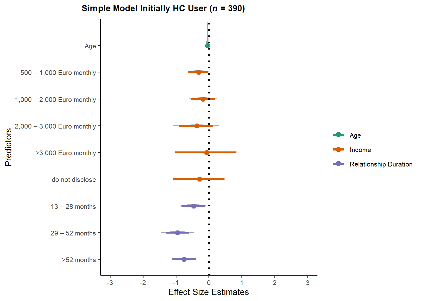

m_selection_congruent_simple_oncenonHC_plot = m_selection_congruent_simple_oncenonHC %>%
  spread_draws(b_age,
               b_net_incomeeuro_500_1000, b_net_incomeeuro_1000_2000, 
               b_net_incomeeuro_2000_3000, b_net_incomeeuro_gt_3000, b_net_incomedont_tell,
               b_relationship_duration_factorPartnered_upto28months,
               b_relationship_duration_factorPartnered_upto52months,
               b_relationship_duration_factorPartnered_morethan52months) %>%
  pivot_longer(cols = c(b_age,
               b_net_incomeeuro_500_1000, b_net_incomeeuro_1000_2000, 
               b_net_incomeeuro_2000_3000, b_net_incomeeuro_gt_3000, b_net_incomedont_tell,
               b_relationship_duration_factorPartnered_upto28months,
               b_relationship_duration_factorPartnered_upto52months,
               b_relationship_duration_factorPartnered_morethan52months),
               names_to = "condition",
               values_to = "r_condition") %>%
  mutate(condition_mean = r_condition,
         group = ifelse(condition %contains% "b_relationship_duration_factor",
                        "Relationship Duration",
                        ifelse(condition %contains% "b_net_income",
                               "Income",
                               NA)),
         condition = ifelse(condition == "b_age", "Age",
                ifelse(condition == "b_net_incomeeuro_500_1000", "500 \U2013 1,000 Euro monthly",
                ifelse(condition == "b_net_incomeeuro_1000_2000", "1,000 \U2013 2,000 Euro monthly",
                ifelse(condition == "b_net_incomeeuro_2000_3000", "2,000 \U2013 3,000 Euro monthly",
                ifelse(condition == "b_net_incomeeuro_gt_3000", ">3,000 Euro monthly",
                ifelse(condition == "b_net_incomedont_tell", "do not disclose",
                ifelse(condition == "b_relationship_duration_factorPartnered_upto12months",
                       "0 \U2013 12 months",
                ifelse(condition == "b_relationship_duration_factorPartnered_upto28months",
                       "13 \U2013 28 months",
                ifelse(condition == "b_relationship_duration_factorPartnered_upto52months",
                       "29 \U2013 52 months",
                ifelse(condition == "b_relationship_duration_factorPartnered_morethan52months",
                       ">52 months",
                       condition)))))))))),
         group = ifelse(is.na(group), condition, group),
         condition = factor(condition, levels = rev(c("Age",
                                        "500 \U2013 1,000 Euro monthly", "1,000 \U2013 2,000 Euro monthly",
                                        "2,000 \U2013 3,000 Euro monthly", ">3,000 Euro monthly", "do not disclose",
                                        "13 \U2013 28 months", "29 \U2013 52 months",
                                        ">52 months")))) %>%
  ggplot(aes(y = condition, x = condition_mean, color = group)) +
  stat_halfeye(.width = .90) +
  geom_vline(xintercept = 0, linetype = "dotted", size = 1) +
  apatheme +
  theme(legend.title = element_blank()) +
  labs(x = "Effect Size Estimates", y = "Predictors") +
  scale_x_continuous(limits = c(-3, 3),
                     breaks= c(-3:3)) +
  scale_color_manual(values = c("#1B9E77", "#D95F02", "#7570B3")) +
  guides(color = guide_legend(override.aes = list(size = 5))) +
  ggtitle(expression(paste(bold("Simple Model Initially Non-HC User ("),
                           bolditalic("n"),
                           bold(" = 384)")))) +
  theme(plot.title = element_text(hjust = -0.35))
m_selection_congruent_simple_oncenonHC_plot

Complex Model

m_selection_congruent_complex_onceHC = brm(congruent_contraception ~
                              age + net_income + relationship_duration_factor +
                              education_years +
                              bfi_extra + bfi_neuro + bfi_agree + bfi_consc + bfi_open +
                              religiosity,
                            data = data %>% filter(contraception_meeting_partner == "yes"),
                            family = bernoulli("probit"),
                            file = "m_selection_congruent_complex_onceHC")

m_selection_congruent_complex_oncenonHC = brm(congruent_contraception ~
                              age + net_income + relationship_duration_factor +
                              education_years +
                              bfi_extra + bfi_neuro + bfi_agree + bfi_consc + bfi_open +
                              religiosity,
                            data = data %>% filter(contraception_meeting_partner == "no"),
                            family = bernoulli("probit"),
                            file = "m_selection_congruent_complex_oncenonHC")

m_selection_congruent_complex_onceHC_plot = m_selection_congruent_complex_onceHC %>%
  spread_draws(b_age,
               b_net_incomeeuro_500_1000, b_net_incomeeuro_1000_2000, 
               b_net_incomeeuro_2000_3000, b_net_incomeeuro_gt_3000, b_net_incomedont_tell,
               b_relationship_duration_factorPartnered_upto28months,
               b_relationship_duration_factorPartnered_upto52months,
               b_relationship_duration_factorPartnered_morethan52months,
               b_education_years,
               b_bfi_extra, b_bfi_neuro, b_bfi_agree, b_bfi_consc, b_bfi_open, 
               b_religiosity) %>%
  pivot_longer(cols = c(b_age,
               b_net_incomeeuro_500_1000, b_net_incomeeuro_1000_2000, 
               b_net_incomeeuro_2000_3000, b_net_incomeeuro_gt_3000, b_net_incomedont_tell,
               b_relationship_duration_factorPartnered_upto28months,
               b_relationship_duration_factorPartnered_upto52months,
               b_relationship_duration_factorPartnered_morethan52months,
               b_education_years,
               b_bfi_extra, b_bfi_neuro, b_bfi_agree, b_bfi_consc, b_bfi_open, 
               b_religiosity),
               names_to = "condition",
               values_to = "r_condition") %>%
  mutate(condition_mean = r_condition,
         group = ifelse(condition %contains% "b_relationship_duration_factor",
                        "Relationship Duration",
                        ifelse(condition %contains% "b_net_income",
                               "Income",
                               NA)),
         condition = ifelse(condition == "b_age", "Age",
                ifelse(condition == "b_net_incomeeuro_500_1000", "500 \U2013 1,000 Euro monthly",
                ifelse(condition == "b_net_incomeeuro_1000_2000", "1,000 \U2013 2,000 Euro monthly",
                ifelse(condition == "b_net_incomeeuro_2000_3000", "2,000 \U2013 3,000 Euro monthly",
                ifelse(condition == "b_net_incomeeuro_gt_3000", ">3,000 Euro monthly",
                ifelse(condition == "b_net_incomedont_tell", "do not disclose",
                ifelse(condition == "b_relationship_duration_factorPartnered_upto12months",
                       "0 \U2013 12 months",
                ifelse(condition == "b_relationship_duration_factorPartnered_upto28months",
                       "13 \U2013 28 months",
                ifelse(condition == "b_relationship_duration_factorPartnered_upto52months",
                       "29 \U2013 52 months",
                ifelse(condition == "b_relationship_duration_factorPartnered_morethan52months",
                       ">52 months",
                ifelse(condition == "b_education_years", "Years of Education",
                ifelse(condition == "b_bfi_extra", "Extraversion",
                ifelse(condition == "b_bfi_neuro", "Neuroticism",
                ifelse(condition == "b_bfi_agree", "Agreeableness",
                ifelse(condition == "b_bfi_consc", "Conscientiousness",
                ifelse(condition == "b_bfi_open", "Openness",
                ifelse(condition == "b_religiosity", "Religiosity",
                       condition))))))))))))))))),
         group = ifelse(is.na(group), condition, group),
         condition = factor(condition, levels = rev(c("Age",
                                        "500 \U2013 1,000 Euro monthly", "1,000 \U2013 2,000 Euro monthly",
                                        "2,000 \U2013 3,000 Euro monthly", ">3,000 Euro monthly", "do not disclose",
                                        "13 \U2013 28 months", "29 \U2013 52 months",
                                        ">52 months",
                                        "Years of Education",
                                        "Extraversion", "Neuroticism", "Agreeableness",
                                         "Conscientiousness","Openness","Religiosity"))),
         group = factor(group, levels = c("Age", "Income", "Relationship Duration",
                                          
                                          "Years of Education",
                                          "Extraversion", "Neuroticism", "Agreeableness",
                                         "Conscientiousness","Openness","Religiosity"))) %>%
  ggplot(aes(y = condition, x = condition_mean, color = group)) +
  stat_halfeye(.width = .90) +
  geom_vline(xintercept = 0, linetype = "dotted", size = 1) +
  apatheme +
  theme(legend.title = element_blank()) +
  labs(x = "Effect Size Estimates", y = "Predictors") +
  scale_x_continuous(limits = c(-3, 3),
                     breaks = c(-3:3)) +
  scale_color_manual(values = c("#1B9E77", "#D95F02", "#7570B3", "#E7298A", "#66A61E",
                                "#E6AB02", "#A6761D", "#0072B2", "#CC79A7", "#56B4E9")) +
  guides(color = guide_legend(override.aes = list(size = 5)))+
  ggtitle(expression(paste(bold("Complex Model Initially HC User ("),
                           bolditalic("n"),
                           bold(" = 390)")))) +
  theme(plot.title = element_text(hjust = -0.35))
m_selection_congruent_complex_onceHC_plot

m_selection_congruent_complex_oncenonHC_plot = m_selection_congruent_complex_oncenonHC %>%
  spread_draws(b_age,
               b_net_incomeeuro_500_1000, b_net_incomeeuro_1000_2000, 
               b_net_incomeeuro_2000_3000, b_net_incomeeuro_gt_3000, b_net_incomedont_tell,
               b_relationship_duration_factorPartnered_upto28months,
               b_relationship_duration_factorPartnered_upto52months,
               b_relationship_duration_factorPartnered_morethan52months,
               b_education_years,
               b_bfi_extra, b_bfi_neuro, b_bfi_agree, b_bfi_consc, b_bfi_open, 
               b_religiosity) %>%
  pivot_longer(cols = c(b_age,
               b_net_incomeeuro_500_1000, b_net_incomeeuro_1000_2000, 
               b_net_incomeeuro_2000_3000, b_net_incomeeuro_gt_3000, b_net_incomedont_tell,
               b_relationship_duration_factorPartnered_upto28months,
               b_relationship_duration_factorPartnered_upto52months,
               b_relationship_duration_factorPartnered_morethan52months,
               b_education_years,
               b_bfi_extra, b_bfi_neuro, b_bfi_agree, b_bfi_consc, b_bfi_open, 
               b_religiosity),
               names_to = "condition",
               values_to = "r_condition") %>%
  mutate(condition_mean = r_condition,
         group = ifelse(condition %contains% "b_relationship_duration_factor",
                        "Relationship Duration",
                        ifelse(condition %contains% "b_net_income",
                               "Income",
                               NA)),
         condition = ifelse(condition == "b_age", "Age",
                ifelse(condition == "b_net_incomeeuro_500_1000", "500 \U2013 1,000 Euro monthly",
                ifelse(condition == "b_net_incomeeuro_1000_2000", "1,000 \U2013 2,000 Euro monthly",
                ifelse(condition == "b_net_incomeeuro_2000_3000", "2,000 \U2013 3,000 Euro monthly",
                ifelse(condition == "b_net_incomeeuro_gt_3000", ">3,000 Euro monthly",
                ifelse(condition == "b_net_incomedont_tell", "do not disclose",
                ifelse(condition == "b_relationship_duration_factorPartnered_upto12months",
                       "0 \U2013 12 months",
                ifelse(condition == "b_relationship_duration_factorPartnered_upto28months",
                       "13 \U2013 28 months",
                ifelse(condition == "b_relationship_duration_factorPartnered_upto52months",
                       "29 \U2013 52 months",
                ifelse(condition == "b_relationship_duration_factorPartnered_morethan52months",
                       ">52 months",
                ifelse(condition == "b_education_years", "Years of Education",
                ifelse(condition == "b_bfi_extra", "Extraversion",
                ifelse(condition == "b_bfi_neuro", "Neuroticism",
                ifelse(condition == "b_bfi_agree", "Agreeableness",
                ifelse(condition == "b_bfi_consc", "Conscientiousness",
                ifelse(condition == "b_bfi_open", "Openness",
                ifelse(condition == "b_religiosity", "Religiosity",
                       condition))))))))))))))))),
         group = ifelse(is.na(group), condition, group),
         condition = factor(condition, levels = rev(c("Age",
                                        "500 \U2013 1,000 Euro monthly", "1,000 \U2013 2,000 Euro monthly",
                                        "2,000 \U2013 3,000 Euro monthly", ">3,000 Euro monthly", "do not disclose",
                                        "13 \U2013 28 months", "29 \U2013 52 months",
                                        ">52 months",
                                        "Years of Education",
                                        "Extraversion", "Neuroticism", "Agreeableness",
                                         "Conscientiousness","Openness","Religiosity"))),
         group = factor(group, levels = c("Age", "Income", "Relationship Duration",
                                          
                                          "Years of Education",
                                          "Extraversion", "Neuroticism", "Agreeableness",
                                         "Conscientiousness","Openness","Religiosity"))) %>%
  ggplot(aes(y = condition, x = condition_mean, color = group)) +
  stat_halfeye(.width = .90) +
  geom_vline(xintercept = 0, linetype = "dotted", size = 1) +
  apatheme +
  theme(legend.title = element_blank()) +
  labs(x = "Effect Size Estimates", y = "Predictors") +
  scale_x_continuous(limits = c(-3, 3),
                     breaks = c(-3:3)) +
  scale_color_manual(values = c("#1B9E77", "#D95F02", "#7570B3", "#E7298A", "#66A61E",
                                "#E6AB02", "#A6761D", "#0072B2", "#CC79A7", "#56B4E9")) +
  guides(color = guide_legend(override.aes = list(size = 5)))+
  ggtitle(expression(paste(bold("Complex Model Initially Non-HC User ("),
                           bolditalic("n"),
                           bold(" = 384)")))) +
  theme(plot.title = element_text(hjust = -0.35))

m_selection_congruent_complex_oncenonHC_plot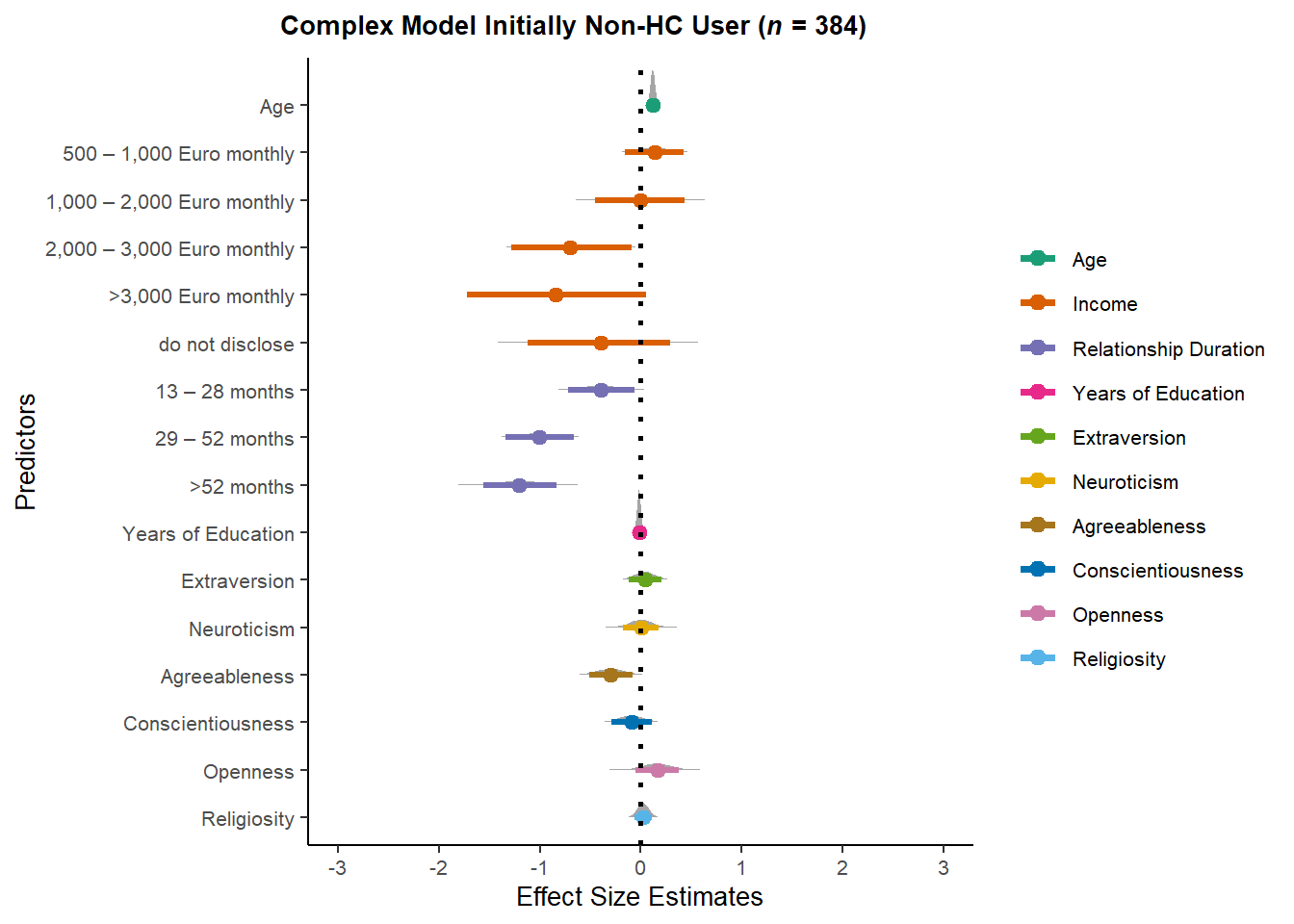

Combine Plots

selection_congruent =
  ggarrange(m_selection_congruent_simple_onceHC_plot +
              theme(legend.position = "none", plot.margin = margin(1,0,0,0,"cm")),
            m_selection_congruent_simple_oncenonHC_plot +
              theme(legend.position = c(0.85,0.5), plot.margin = margin(1,0,0,0,"cm")),
            m_selection_congruent_complex_onceHC_plot +
              theme(legend.position = "none", plot.margin = margin(1,0,0,0,"cm")),
            m_selection_congruent_complex_oncenonHC_plot  +
              theme(legend.position = c(0.85,0.5), plot.margin = margin(1,0,0,0,"cm")),
          hjust = -0.1, vjust = 1.1,
          ncol = 2, nrow = 2,
          align = "v")

selection_congruent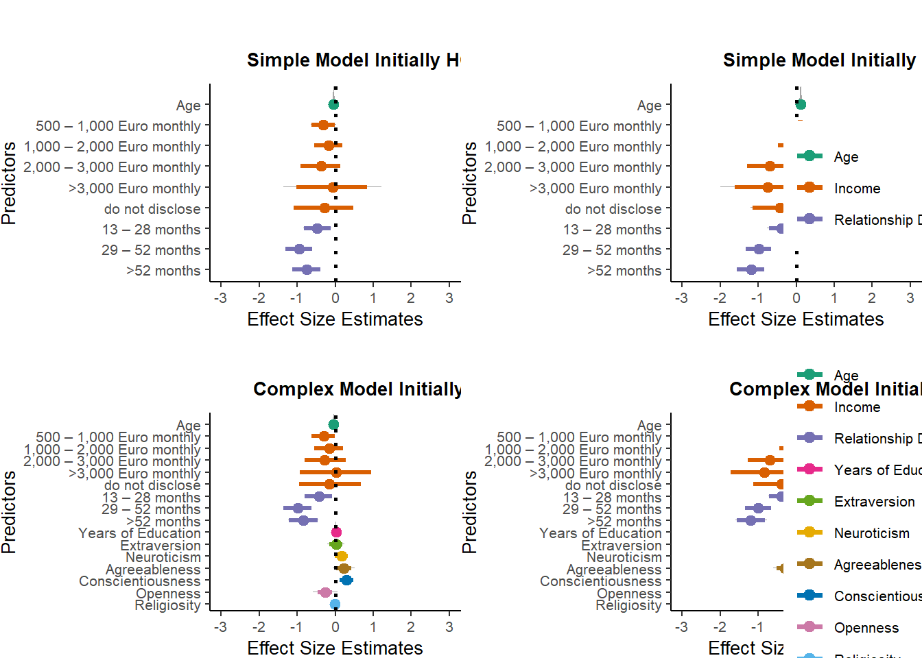

jpeg('Effect size estimates for models with congruency in contraceptive method as an outcome.jpg', 
     width = 1600, height = 720, quality = 100)
selection_congruent
dev.off()

## png 
##   2

Effects of Hormonal Contraceptives

Uncontrolled

Models

m_hc_atrr = brm(attractiveness_partner ~ contraception_hormonal,
                data = data, family = gaussian(),
                file = "m_hc_atrr")
m_hc_relsat = brm(relationship_satisfaction ~ contraception_hormonal,
                data = data, family = gaussian(),
                file = "m_hc_relsat")
m_hc_sexsat = brm(satisfaction_sexual_intercourse ~ contraception_hormonal,
                data = data, family = gaussian(),
                file = "m_hc_sexsat")
m_hc_libido = brm(diary_libido_mean ~ contraception_hormonal,
                data = data, family = gaussian(),
                file = "m_hc_libido")
m_hc_sexfreqpen = brm(diary_sex_active_sex_sum ~
                        offset(log(number_of_days)) +
                        contraception_hormonal,
                data = data, family = poisson(),
                file = "mrobust_hc_sexfreqpen")
m_hc_masfreq = brm(diary_masturbation_sum ~ offset(log(number_of_days)) +
                     contraception_hormonal,
                data = data, family = poisson(),
                file = "mrobust_hc_masfreq")

Forest Plot for Effect Sizes

models = rbind(
  m_hc_atrr %>%
    spread_draws(b_contraception_hormonalyes) %>%
    pivot_longer(cols = c(b_contraception_hormonalyes),
                 names_to = "condition",
                 values_to = "r_condition") %>%
    mutate(model = "Perceived Partner Attractiveness\nROPE = [-0.07, 0.07]",
           ROPE = 0.07),
  m_hc_relsat %>%
    spread_draws(b_contraception_hormonalyes) %>%
    pivot_longer(cols = c(b_contraception_hormonalyes),
                 names_to = "condition",
                 values_to = "r_condition") %>%
    mutate(model = "Relationship Satisfaction\nROPE = [-0.04, 0.04]",
           ROPE = 0.04),
  m_hc_sexsat %>%
    spread_draws(b_contraception_hormonalyes) %>%
    pivot_longer(cols = c(b_contraception_hormonalyes),
                 names_to = "condition",
                 values_to = "r_condition") %>%
    mutate(model = "Sexual Satisfaction\nROPE = [-0.11, 0.11]",
           ROPE = 0.11),
  m_hc_libido %>%
    spread_draws(b_contraception_hormonalyes) %>%
    pivot_longer(cols = c(b_contraception_hormonalyes),
                 names_to = "condition",
                 values_to = "r_condition") %>%
    mutate(model = "Libido\nROPE = [-0.06, 0.06]",
           ROPE = 0.06),
  m_hc_sexfreqpen %>%
    spread_draws(b_contraception_hormonalyes) %>%
    pivot_longer(cols = c(b_contraception_hormonalyes),
                 names_to = "condition",
                 values_to = "r_condition") %>%
    mutate(model = "Frequency of Vaginal Intercourse\nROPE = [-0.05, 0.05]",
           ROPE = 0.05),
  m_hc_masfreq %>%
    spread_draws(b_contraception_hormonalyes) %>%
    pivot_longer(cols = c(b_contraception_hormonalyes),
                 names_to = "condition",
                 values_to = "r_condition") %>%
    mutate(model = "Frequency of Masturbation\nROPE = [-0.05, 0.05]",
           ROPE = 0.05))

data1 = models %>%
  mutate(model = factor(model,
                   levels = c("Frequency of Masturbation\nROPE = [-0.05, 0.05]",
                              "Frequency of Vaginal Intercourse\nROPE = [-0.05, 0.05]",
                              "Libido\nROPE = [-0.06, 0.06]",
                              "Sexual Satisfaction\nROPE = [-0.11, 0.11]",
                              "Relationship Satisfaction\nROPE = [-0.04, 0.04]",
                              "Perceived Partner Attractiveness\nROPE = [-0.07, 0.07]")))
data2 = models %>%
  group_by(model, ROPE) %>%
  mutate(model = factor(model,
                        levels = c("Frequency of Masturbation\nROPE = [-0.05, 0.05]",
                                   "Frequency of Vaginal Intercourse\nROPE = [-0.05, 0.05]",
                                   "Libido\nROPE = [-0.06, 0.06]",
                                   "Sexual Satisfaction\nROPE = [-0.11, 0.11]",
                                   "Relationship Satisfaction\nROPE = [-0.04, 0.04]",
                                   "Perceived Partner Attractiveness\nROPE = [-0.07, 0.07]"))) %>%
  mean_qi(condition_mean = r_condition,
          .width = c(.90)) %>%
  mutate(text = ifelse(.width == .90,
                       str_c(round(condition_mean, 2),
                             " [",
                             round(.lower, 2),
                             "; ",
                             round(.upper, 2),
                             "]"), NA),
         sig = ifelse(.lower > ROPE | .upper < -ROPE, T, F))


hc_uncontrolled = ggplot() +
  stat_halfeye(data = data1,
               aes(y = model, x = r_condition,
                   color = "grey"),
               .width = .90) +
  geom_vline(xintercept = 0, linetype = "dotted") +
  geom_pointinterval(data = data2,
                     aes(y = model,
                         x = condition_mean,
                         xmin = .lower,
                         xmax = .upper,
                         color = sig)) +
  geom_point(data = data1, aes(y = model, x = ROPE), shape = "|", size = 10, color = "black") +
  geom_point(data = data1, aes(y = model, x = -ROPE), shape = "|", size = 10, color = "black") +
  geom_point(data = data1, aes(y = model, x = ROPE), shape = 58, size = 10, color = "white") +
  geom_point(data = data1, aes(y = model, x = -ROPE), shape = 58, size = 10, color = "white") +
  apatheme +
  scale_color_manual(data2, values = c("skyblue", "grey", "red")) +
  scale_x_continuous(breaks = c(-0.5, -0.4, -0.3, -0.2, -0.1, 0, 0.1, 0.2, 0.3, 0.4, 0.5),
                     limits = c(-0.5, 0.5)) +
  labs(x = "Effect Size Estimates of Hormonal Contraception", y = "Outcomes") +
  theme(legend.position = "none")
hc_uncontrolled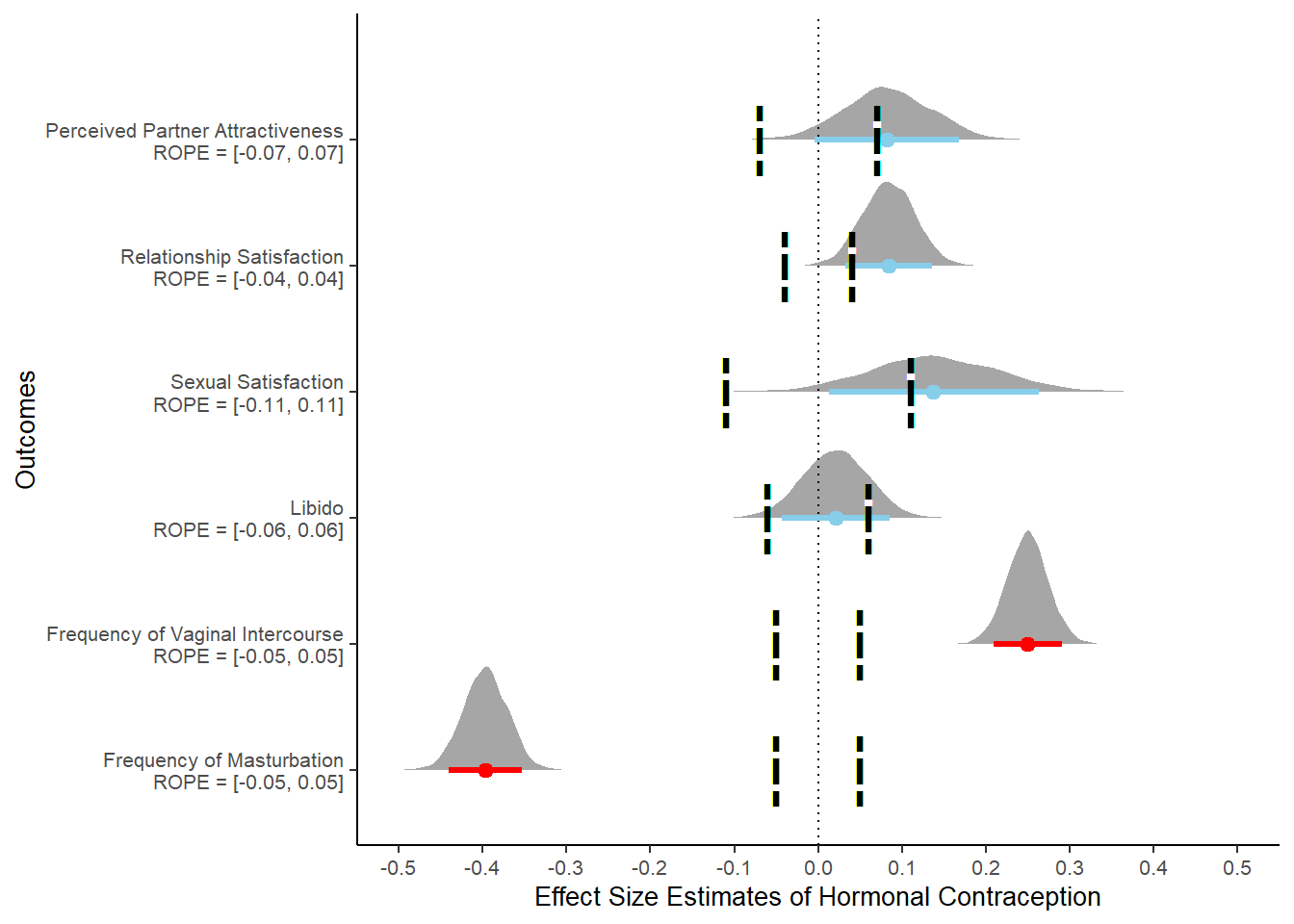

Controlled

Models

m_hc_atrr_controlled = brm(attractiveness_partner ~ contraception_hormonal +
                             age + net_income + relationship_duration_factor +
                              education_years +
                              bfi_extra + bfi_neuro + bfi_agree + bfi_consc + bfi_open +
                              religiosity,
                data = data, family = gaussian(),
                file = "m_hc_atrr_controlled")

m_hc_relsat_controlled = brm(relationship_satisfaction ~ contraception_hormonal +
                             age + net_income + relationship_duration_factor +
                              education_years +
                              bfi_extra + bfi_neuro + bfi_agree + bfi_consc + bfi_open +
                              religiosity,
                data = data, family = gaussian(),
                file = "m_hc_relsat_controlled")

m_hc_sexsat_controlled = brm(satisfaction_sexual_intercourse ~ contraception_hormonal +
                             age + net_income + relationship_duration_factor +
                              education_years +
                              bfi_extra + bfi_neuro + bfi_agree + bfi_consc + bfi_open +
                              religiosity,
                data = data, family = gaussian(),
                file = "m_hc_sexsat_controlled")

m_hc_libido_controlled = brm(diary_libido_mean ~ contraception_hormonal +
                             age + net_income + relationship_duration_factor +
                              education_years +
                              bfi_extra + bfi_neuro + bfi_agree + bfi_consc + bfi_open +
                              religiosity,
                data = data, family = gaussian(),
                file = "m_hc_libido_controlled")

m_hc_sexfreqpen_controlled = brm(diary_sex_active_sex_sum ~
                        offset(log(number_of_days)) +
                        contraception_hormonal +
                        age + net_income + relationship_duration_factor +
                              education_years +
                              bfi_extra + bfi_neuro + bfi_agree + bfi_consc + bfi_open +
                              religiosity,
                data = data, family = poisson(),
                file = "mrobust_hc_sexfreqpen_controlled")

m_hc_masfreq_controlled = brm(diary_masturbation_sum ~
                        offset(log(number_of_days)) +
                        contraception_hormonal +
                        age + net_income + relationship_duration_factor +
                              education_years +
                              bfi_extra + bfi_neuro + bfi_agree + bfi_consc + bfi_open +
                              religiosity,
                data = data, family = poisson(),
                file = "mrobust_hc_masfreq_controlled")

Forest Plot for Effect Sizes

models = rbind(
  m_hc_atrr_controlled %>%
    spread_draws(b_contraception_hormonalyes) %>%
    pivot_longer(cols = c(b_contraception_hormonalyes),
                 names_to = "condition",
                 values_to = "r_condition") %>%
    mutate(model = "Perceived Partner Attractiveness\nROPE = [-0.07, 0.07]",
           ROPE = 0.07),
  m_hc_relsat_controlled %>%
    spread_draws(b_contraception_hormonalyes) %>%
    pivot_longer(cols = c(b_contraception_hormonalyes),
                 names_to = "condition",
                 values_to = "r_condition") %>%
    mutate(model = "Relationship Satisfaction\nROPE = [-0.04, 0.04]",
           ROPE = 0.04),
  m_hc_sexsat_controlled %>%
    spread_draws(b_contraception_hormonalyes) %>%
    pivot_longer(cols = c(b_contraception_hormonalyes),
                 names_to = "condition",
                 values_to = "r_condition") %>%
    mutate(model = "Sexual Satisfaction\nROPE = [-0.11, 0.11]",
           ROPE = 0.11),
  m_hc_libido_controlled %>%
    spread_draws(b_contraception_hormonalyes) %>%
    pivot_longer(cols = c(b_contraception_hormonalyes),
                 names_to = "condition",
                 values_to = "r_condition") %>%
    mutate(model = "Libido\nROPE = [-0.06, 0.06]",
           ROPE = 0.06),
  m_hc_sexfreqpen_controlled %>%
    spread_draws(b_contraception_hormonalyes) %>%
    pivot_longer(cols = c(b_contraception_hormonalyes),
                 names_to = "condition",
                 values_to = "r_condition") %>%
    mutate(model = "Frequency of Vaginal Intercourse\nROPE = [-0.05, 0.05]",
           ROPE = 0.05),
  m_hc_masfreq_controlled %>%
    spread_draws(b_contraception_hormonalyes) %>%
    pivot_longer(cols = c(b_contraception_hormonalyes),
                 names_to = "condition",
                 values_to = "r_condition") %>%
    mutate(model = "Frequency of Masturbation\nROPE = [-0.05, 0.05]",
           ROPE = 0.05))

data1 = models %>%
  mutate(model = factor(model,
                   levels = c("Frequency of Masturbation\nROPE = [-0.05, 0.05]",
                              "Frequency of Vaginal Intercourse\nROPE = [-0.05, 0.05]",
                              "Libido\nROPE = [-0.06, 0.06]",
                              "Sexual Satisfaction\nROPE = [-0.11, 0.11]",
                              "Relationship Satisfaction\nROPE = [-0.04, 0.04]",
                              "Perceived Partner Attractiveness\nROPE = [-0.07, 0.07]")))
data2 = models %>%
  group_by(model, ROPE) %>%
  mutate(model = factor(model,
                        levels = c("Frequency of Masturbation\nROPE = [-0.05, 0.05]",
                                   "Frequency of Vaginal Intercourse\nROPE = [-0.05, 0.05]",
                                   "Libido\nROPE = [-0.06, 0.06]",
                                   "Sexual Satisfaction\nROPE = [-0.11, 0.11]",
                                   "Relationship Satisfaction\nROPE = [-0.04, 0.04]",
                                   "Perceived Partner Attractiveness\nROPE = [-0.07, 0.07]"))) %>%
  mean_qi(condition_mean = r_condition,
          .width = c(.90)) %>%
  mutate(text = ifelse(.width == .90,
                       str_c(round(condition_mean, 2),
                             " [",
                             round(.lower, 2),
                             "; ",
                             round(.upper, 2),
                             "]"), NA),
         sig = ifelse(.lower > ROPE | .upper < -ROPE, "declined",
                      ifelse(abs(.lower) < ROPE  & .upper > ROPE, "undecidable", "accepted")))


hc_controlled = ggplot() +
  stat_halfeye(data = data1,
               aes(y = model, x = r_condition,
                   color = "grey"),
               .width = .90) +
  geom_vline(xintercept = 0, linetype = "dotted") +
  geom_pointinterval(data = data2,
                     aes(y = model,
                         x = condition_mean,
                         xmin = .lower,
                         xmax = .upper,
                         color = sig)) +
  geom_point(data = data1, aes(y = model, x = ROPE), shape = "|", size = 10, color = "black") +
  geom_point(data = data1, aes(y = model, x = -ROPE), shape = "|", size = 10, color = "black") +
  geom_point(data = data1, aes(y = model, x = ROPE), shape = 58, size = 10, color = "white") +
  geom_point(data = data1, aes(y = model, x = -ROPE), shape = 58, size = 10, color = "white") +
  apatheme +
  theme(legend.position = "none") +
  scale_color_manual(values = c("red", "green", "skyblue", "grey")) +
  scale_x_continuous(breaks = c(-0.5, -0.4, -0.3, -0.2, -0.1, 0, 0.1, 0.2, 0.3, 0.4, 0.5),
                     limits = c(-0.5, 0.5)) +
  labs(x = "Effect Size Estimates of Hormonal Contraception", y = "Outcomes")  +
  theme(legend.position = "none")
hc_controlled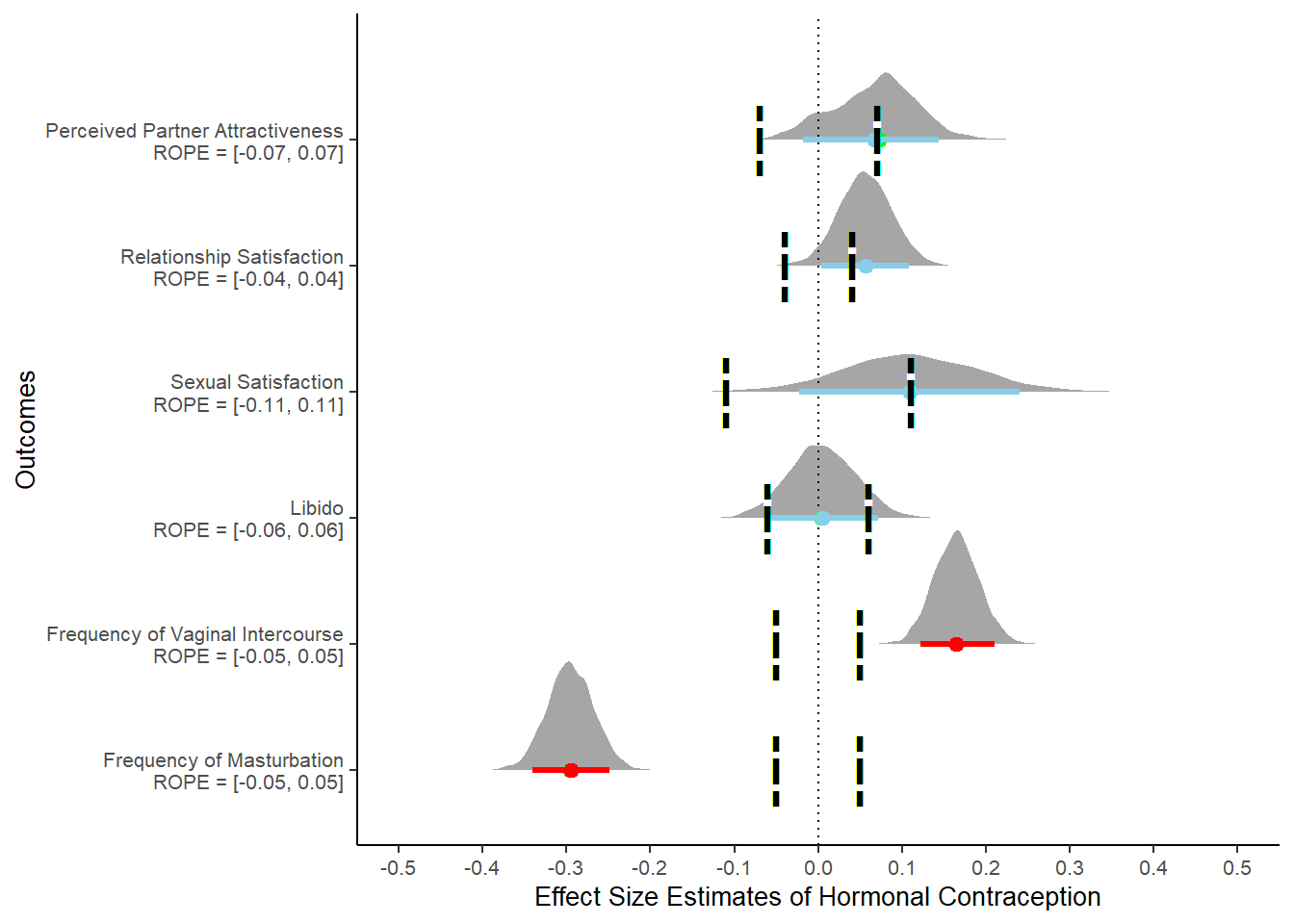

Combine Plots

hc_plots =
  ggarrange(hc_uncontrolled + theme(plot.margin = margin(1,0,0,0,"cm")),
            hc_controlled + theme(plot.margin = margin(3,0,0,0,"cm")),
          labels = c("Uncontrolled Model", "\nControlled Model"),
          font.label = list(size = 20, color = "black", face = "bold", family = "sans"),
          hjust = -0.1,
          ncol = 1, nrow = 2,
          align = "v")

hc_plots

jpeg('Effect size estimates for hormonal contraceptives on outcomes.jpg', 
     width = 800, height = 1000, quality = 100)
hc_plots
dev.off()

## png 
##   2

Effects of (in)congruent use of hormonal contraceptives

Plots

m_congruency_atrr = brm(attractiveness_partner ~
                          contraception_hormonal * congruent_contraception,
                data = data, family = gaussian(),
                file = "m_congruency_atrr")

m_congruency_atrr_ce = m_congruency_atrr %>% 
  conditional_effects(., effects = "contraception_hormonal:congruent_contraception",
                    prob = 0.90)

m_congruency_atrr_plot = 
  plot(m_congruency_atrr_ce, plot = FALSE)[[1]] +
  labs(x = "Current Contraceptive Method",
       y = "Perceived Partner Attractiveness") +
  scale_x_discrete(labels=c("Non-HC", "HC")) +
  scale_color_manual(name = "Congruent Contraceptive Method", labels = c("No", "Yes"),
                     values=c("#D95F02", "#1B9E77")) +
  scale_fill_manual(name = "Congruent Contraceptive Method", labels = c("No", "Yes"),
                    values=c("#D95F02", "#1B9E77")) +
  apatheme

m_congruency_atrr_plot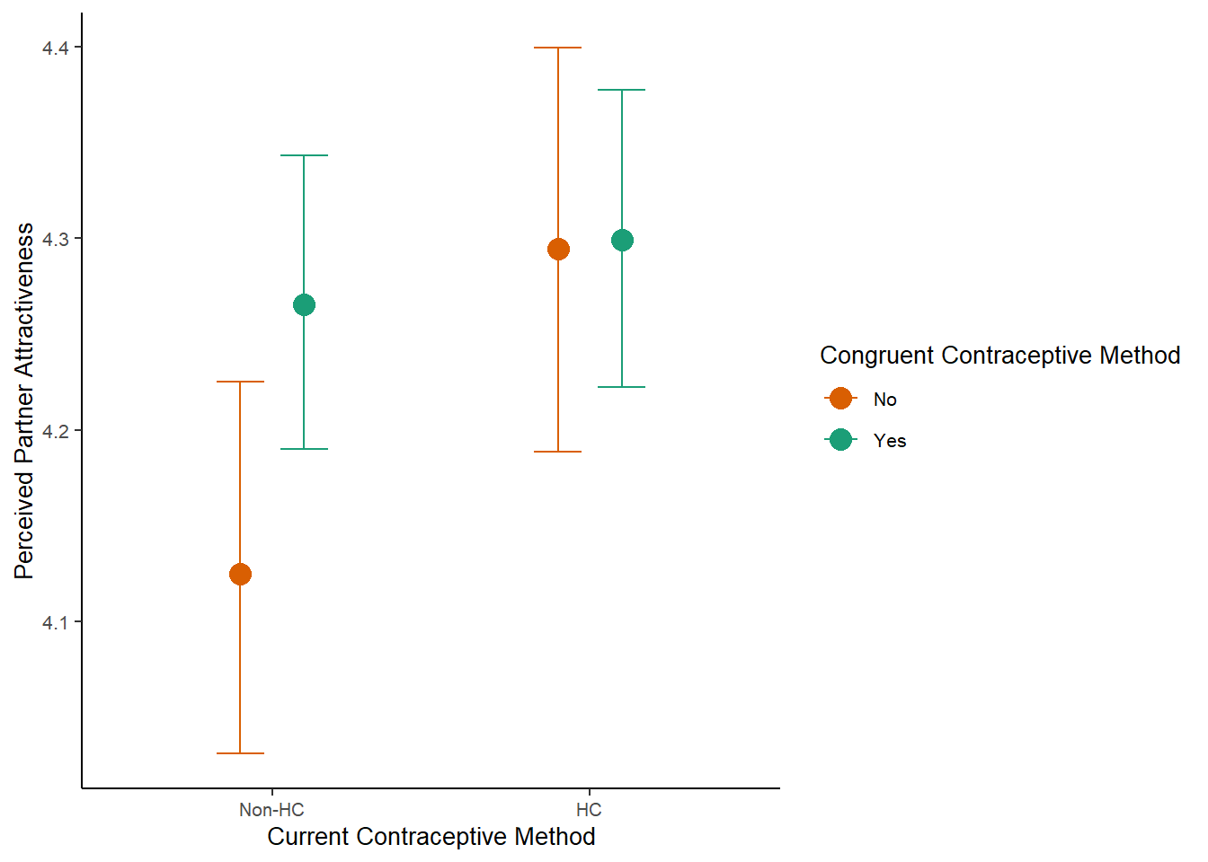

 m_congruency_relsat = brm(relationship_satisfaction ~
                          contraception_hormonal * congruent_contraception,
                data = data, family = gaussian(),
                file = "m_congruency_relsat")

m_congruency_relsat_ce = m_congruency_relsat %>% 
  conditional_effects(., effects = "contraception_hormonal:congruent_contraception",
                    prob = 0.90)

m_congruency_relsat_plot = 
  plot(m_congruency_relsat_ce, plot = FALSE)[[1]] +
  labs(x = "Current Contraceptive Method",
       y = "Relationship Satisfaction") +
  scale_x_discrete(labels=c("Non-HC", "HC")) +
  scale_color_manual(name = "Congruent Contraceptive Method", labels = c("No", "Yes"),
                     values=c("#D95F02", "#1B9E77")) +
  scale_fill_manual(name = "Congruent Contraceptive Method", labels = c("No", "Yes"),
                    values=c("#D95F02", "#1B9E77")) +
  apatheme

m_congruency_relsat_plot

m_congruency_sexsat = brm(satisfaction_sexual_intercourse ~
                          contraception_hormonal * congruent_contraception,
                data = data, family = gaussian(),
                file = "m_congruency_sexsat")


m_congruency_sexsat_ce = m_congruency_sexsat %>% 
  conditional_effects(., effects = "contraception_hormonal:congruent_contraception",
                    prob = 0.90)

m_congruency_sexsat_plot = 
  plot(m_congruency_sexsat_ce, plot = FALSE)[[1]] +
  labs(x = "Current Contraceptive Method",
       y = "Sexual Satisfaction") +
  scale_x_discrete(labels=c("Non-HC", "HC")) +
  scale_color_manual(name = "Congruent Contraceptive Method", labels = c("No", "Yes"),
                     values=c("#D95F02", "#1B9E77")) +
  scale_fill_manual(name = "Congruent Contraceptive Method", labels = c("No", "Yes"),
                    values=c("#D95F02", "#1B9E77")) +
  apatheme

m_congruency_sexsat_plot

m_congruency_libido = brm(diary_libido_mean ~
                          contraception_hormonal * congruent_contraception,
                data = data, family = gaussian(),
                file = "m_congruency_libido")

m_congruency_libido_ce = m_congruency_libido %>% 
  conditional_effects(., effects = "contraception_hormonal:congruent_contraception",
                    prob = 0.90)

m_congruency_libido_plot = 
  plot(m_congruency_libido_ce, plot = FALSE)[[1]] +
  labs(x = "Current Contraceptive Method",
       y = "Libido") +
  scale_x_discrete(labels=c("Non-HC", "HC")) +
  scale_color_manual(name = "Congruent Contraceptive Method", labels = c("No", "Yes"),
                     values=c("#D95F02", "#1B9E77")) +
  scale_fill_manual(name = "Congruent Contraceptive Method", labels = c("No", "Yes"),
                    values=c("#D95F02", "#1B9E77")) +
  apatheme

m_congruency_libido_plot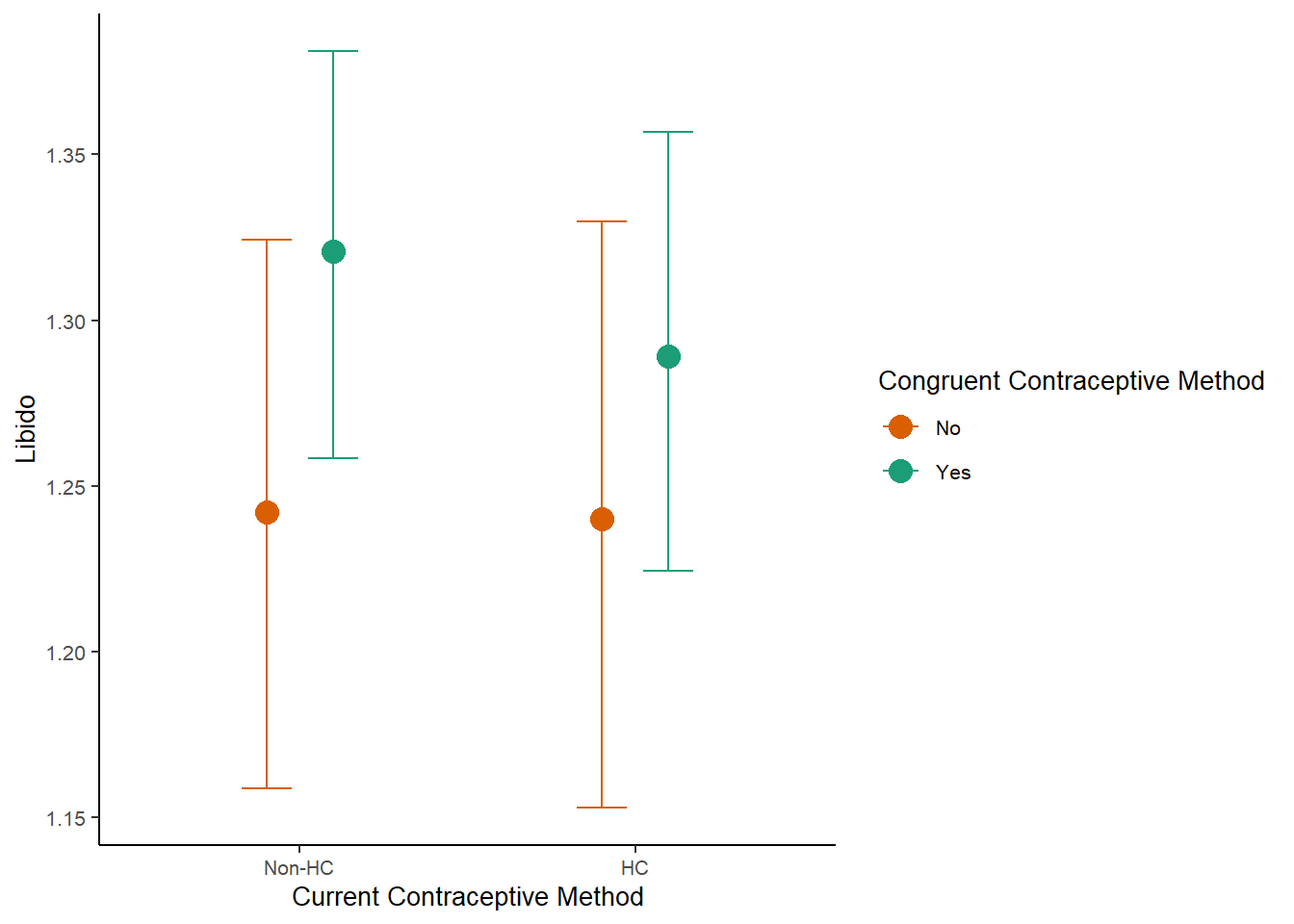

m_congruency_sexfreqpen = brm(diary_sex_active_sex_sum ~ offset(log(number_of_days)) +
                     contraception_hormonal * congruent_contraception,
                data = data, family = poisson(),
                file = "mrobust_congruency_sexfreqpen")


m_congruency_sexfreqpen_ce = m_congruency_sexfreqpen %>% 
  conditional_effects(., effects = "contraception_hormonal:congruent_contraception",
                    prob = 0.90,
                    conditions = data.frame(number_of_days = 1))

m_congruency_sexfreqpen_plot = 
  plot(m_congruency_sexfreqpen_ce, plot = FALSE)[[1]] +
  labs(x = "Current Contraceptive Method",
       y = "Frequency of Vaginal Intercourse\n(Probablity per Day)") +
  scale_x_discrete(labels=c("Non-HC", "HC")) +
  scale_color_manual(name = "Congruent Contraceptive Method", labels = c("No", "Yes"),
                     values=c("#D95F02", "#1B9E77")) +
  scale_fill_manual(name = "Congruent Contraceptive Method", labels = c("No", "Yes"),
                    values=c("#D95F02", "#1B9E77")) +
  apatheme 

m_congruency_sexfreqpen_plot

m_congruency_masfreq = brm(diary_masturbation_sum ~ offset(log(number_of_days)) +
                             contraception_hormonal * congruent_contraception,
                data = data, family = poisson(),
                file = "mrobust_congruency_masfreq")

m_congruency_masfreq_ce = m_congruency_masfreq %>% 
  conditional_effects(., effects = "contraception_hormonal:congruent_contraception",
                    prob = 0.90,
                    conditions = data.frame(number_of_days = 1))

m_congruency_masfreq_plot = 
  plot(m_congruency_masfreq_ce, plot = FALSE)[[1]] +
  labs(x = "Current Contraceptive Method",
       y = "Frequency of Masturbation\n(Probablity per Day)") +
  scale_x_discrete(labels=c("Non-HC", "HC")) +
  scale_color_manual(name = "Congruent Contraceptive Method", labels = c("No", "Yes"),
                     values=c("#D95F02", "#1B9E77")) +
  scale_fill_manual(name = "Congruent Contraceptive Method", labels = c("No", "Yes"),
                    values=c("#D95F02", "#1B9E77")) +
  apatheme

m_congruency_masfreq_plot

Combine Plots

congruency_uncontrolled =
  ggarrange(m_congruency_atrr_plot +
              rremove("xlab"),
            m_congruency_relsat_plot +
              rremove("xlab"),
            m_congruency_sexsat_plot +
              rremove("xlab"),
            m_congruency_libido_plot +
              rremove("xlab"),
            m_congruency_sexfreqpen_plot,
            m_congruency_masfreq_plot,
          common.legend = TRUE, legend = "bottom",
          ncol = 2, nrow = 3,
          align = "v")

congruency_uncontrolled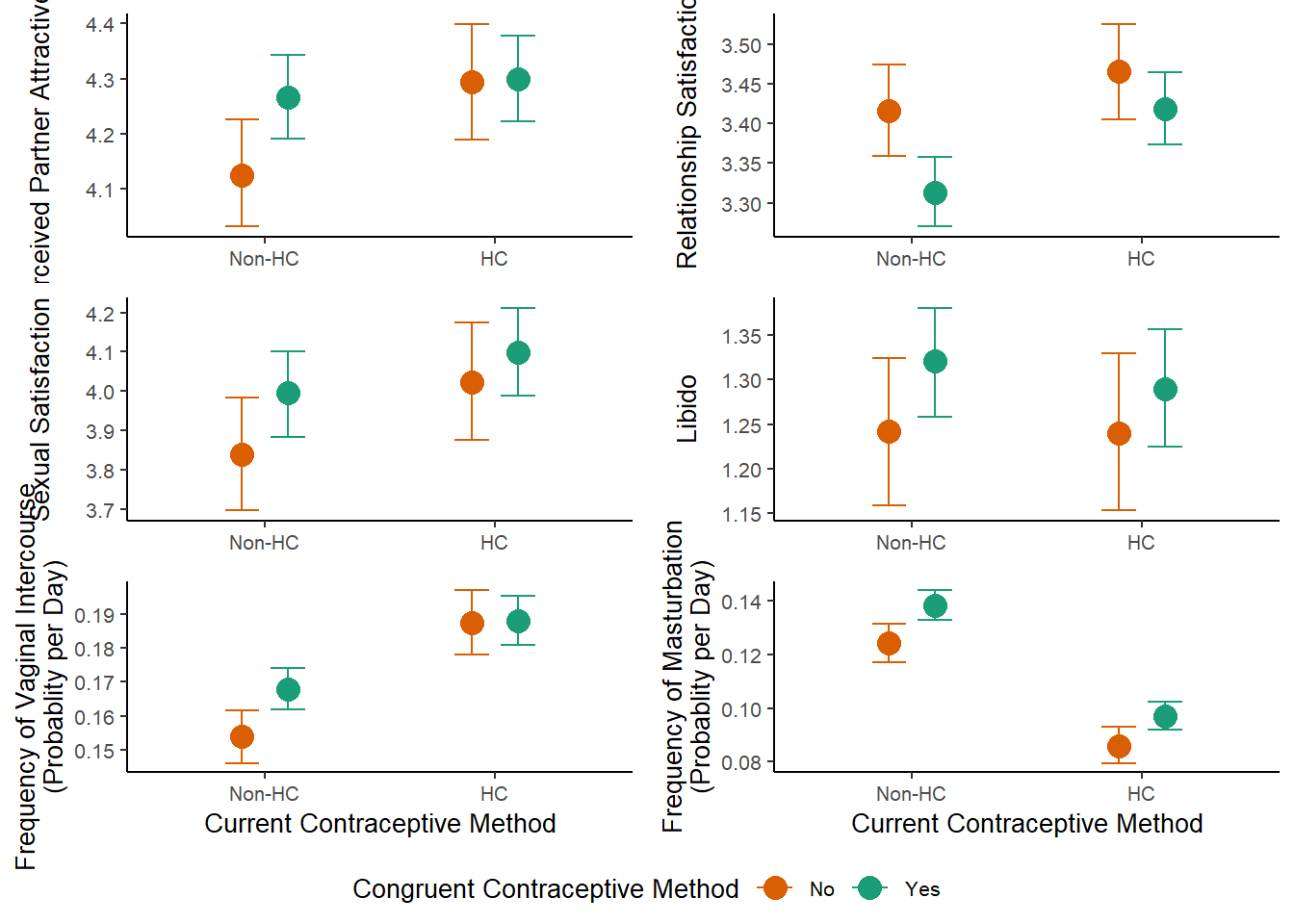

jpeg('Differences in current contraceptive method, congruent use of contraceptive method, and their interaction.jpg', 
     width = 800, height = 1000, quality = 100)
congruency_uncontrolled
dev.off()

## png 
##   2

Controlled effects of (in)congruent use of hormonal contraceptives

Plots

m_congruency_atrr_controlled = brm(attractiveness_partner ~
                          contraception_hormonal * congruent_contraception +
                             age + net_income + relationship_duration_factor +
                              education_years +
                              bfi_extra + bfi_neuro + bfi_agree + bfi_consc + bfi_open +
                              religiosity,
                data = data, family = gaussian(),
                file = "m_congruency_atrr_controlled")

m_congruency_atrr_controlled_ce = m_congruency_atrr_controlled %>% 
  conditional_effects(., effects = "contraception_hormonal:congruent_contraception",
                    prob = 0.90)

m_congruency_atrr_controlled_plot = 
  plot(m_congruency_atrr_controlled_ce, plot = FALSE)[[1]] +
  labs(x = "Current Contraceptive Method",
       y = "Perceived Partner Attractiveness") +
  scale_x_discrete(labels=c("Non-HC", "HC")) +
  scale_color_manual(name = "Congruent Contraceptive Method", labels = c("No", "Yes"),
                     values=c("#D95F02", "#1B9E77")) +
  scale_fill_manual(name = "Congruent Contraceptive Method", labels = c("No", "Yes"),
                    values=c("#D95F02", "#1B9E77")) +
  apatheme

m_congruency_atrr_controlled_plot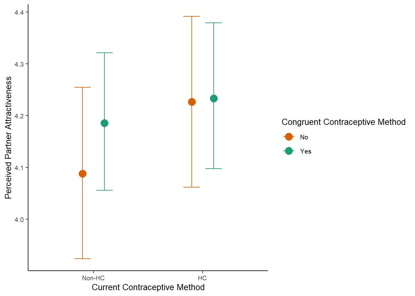

m_congruency_relsat_controlled = brm(relationship_satisfaction ~
                          contraception_hormonal * congruent_contraception +
                             age + net_income + relationship_duration_factor +
                              education_years +
                              bfi_extra + bfi_neuro + bfi_agree + bfi_consc + bfi_open +
                              religiosity,
                data = data, family = gaussian(),
                file = "m_congruency_relsat_controlled")

m_congruency_relsat_controlled_ce = m_congruency_relsat_controlled %>% 
  conditional_effects(., effects = "contraception_hormonal:congruent_contraception",
                    prob = 0.90)

m_congruency_relsat_controlled_plot = 
  plot(m_congruency_relsat_controlled_ce, plot = FALSE)[[1]] +
  labs(x = "Current Contraceptive Method",
       y = "Relationship Satisfaction") +
  scale_x_discrete(labels=c("Non-HC", "HC")) +
  scale_color_manual(name = "Congruent Contraceptive Method", labels = c("No", "Yes"),
                     values=c("#D95F02", "#1B9E77")) +
  scale_fill_manual(name = "Congruent Contraceptive Method", labels = c("No", "Yes"),
                    values=c("#D95F02", "#1B9E77")) +
  apatheme 

m_congruency_relsat_controlled_plot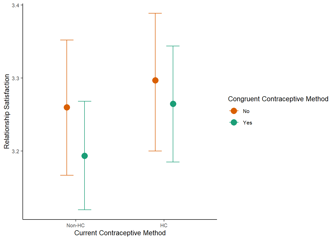

m_congruency_sexsat_controlled = brm(satisfaction_sexual_intercourse ~
                          contraception_hormonal * congruent_contraception +
                             age + net_income + relationship_duration_factor +
                              education_years +
                              bfi_extra + bfi_neuro + bfi_agree + bfi_consc + bfi_open +
                              religiosity,
                data = data, family = gaussian(),
                file = "m_congruency_sexsat_controlled")

m_congruency_sexsat_controlled_ce = m_congruency_sexsat_controlled %>% 
  conditional_effects(., effects = "contraception_hormonal:congruent_contraception",
                    prob = 0.90)

m_congruency_sexsat_controlled_plot = 
  plot(m_congruency_sexsat_controlled_ce, plot = FALSE)[[1]] +
  labs(x = "Current Contraceptive Method",
       y = "Sexual Satisfaction") +
  scale_x_discrete(labels=c("Non-HC", "HC")) +
  scale_color_manual(name = "Congruent Contraceptive Method", labels = c("No", "Yes"),
                     values=c("#D95F02", "#1B9E77")) +
  scale_fill_manual(name = "Congruent Contraceptive Method", labels = c("No", "Yes"),
                    values=c("#D95F02", "#1B9E77")) +
  apatheme 

m_congruency_sexsat_controlled_plot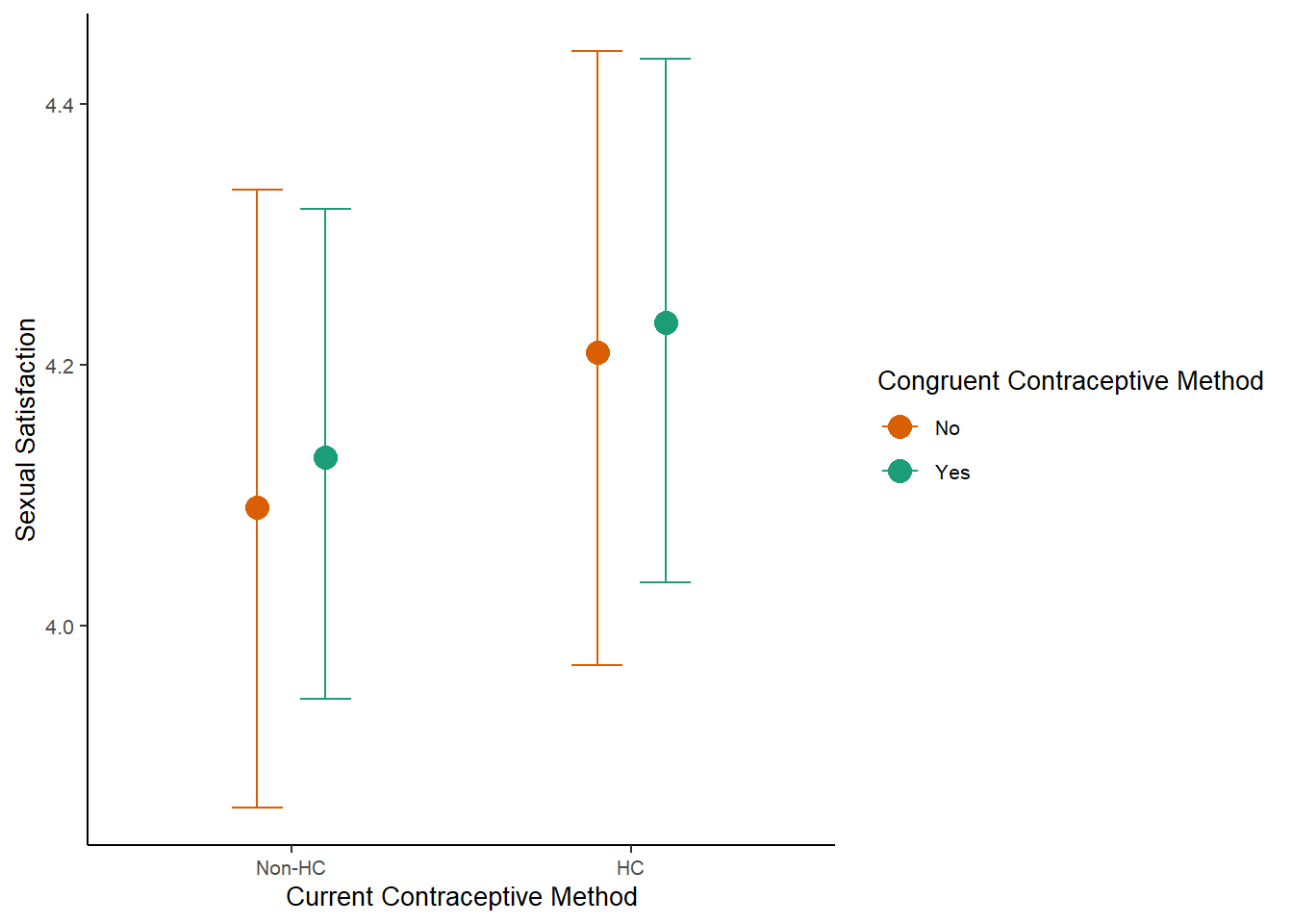

m_congruency_libido_controlled = brm(diary_libido_mean ~
                          contraception_hormonal * congruent_contraception +
                             age + net_income + relationship_duration_factor +
                              education_years +
                              bfi_extra + bfi_neuro + bfi_agree + bfi_consc + bfi_open +
                              religiosity,
                data = data, family = gaussian(),
                file = "m_congruency_libido_controlled")

m_congruency_libido_controlled_ce = m_congruency_libido_controlled %>% 
  conditional_effects(., effects = "contraception_hormonal:congruent_contraception",
                    prob = 0.90)

m_congruency_libido_controlled_plot = 
  plot(m_congruency_libido_controlled_ce, plot = FALSE)[[1]] +
  labs(x = "Current Contraceptive Method",
       y = "Libido") +
  scale_x_discrete(labels=c("Non-HC", "HC")) +
  scale_color_manual(name = "Congruent Contraceptive Method", labels = c("No", "Yes"),
                     values=c("#D95F02", "#1B9E77")) +
  scale_fill_manual(name = "Congruent Contraceptive Method", labels = c("No", "Yes"),
                    values=c("#D95F02", "#1B9E77")) +
  apatheme 

m_congruency_libido_controlled_plot

m_congruency_sexfreqpen_controlled = brm(diary_sex_active_sex_sum ~
                        offset(log(number_of_days)) +
                        contraception_hormonal * congruent_contraception +
                        age + net_income + relationship_duration_factor +
                              education_years +
                              bfi_extra + bfi_neuro + bfi_agree + bfi_consc + bfi_open +
                              religiosity,
                data = data, family = poisson(),
                file = "mrobust_congruency_sexfreqpen_controlled")

m_congruency_sexfreqpen_controlled_ce = m_congruency_sexfreqpen_controlled %>% 
  conditional_effects(., effects = "contraception_hormonal:congruent_contraception",
                    prob = 0.90,
                    conditions = data.frame(number_of_days = 1))

m_congruency_sexfreqpen_controlled_plot = 
  plot(m_congruency_sexfreqpen_controlled_ce, plot = FALSE)[[1]] +
  labs(x = "Current Contraceptive Method",
       y = "Frequency of Vaginal Intercourse\n(Probability per Day)") +
  scale_x_discrete(labels=c("Non-HC", "HC")) +
  scale_color_manual(name = "Congruent Contraceptive Method", labels = c("No", "Yes"),
                     values=c("#D95F02", "#1B9E77")) +
  scale_fill_manual(name = "Congruent Contraceptive Method", labels = c("No", "Yes"),
                    values=c("#D95F02", "#1B9E77")) +
  apatheme 

m_congruency_sexfreqpen_controlled_plot

m_congruency_masfreq_controlled = brm(diary_masturbation_sum ~
                        offset(log(number_of_days)) +
                        contraception_hormonal * congruent_contraception +
                        age + net_income + relationship_duration_factor +
                              education_years +
                              bfi_extra + bfi_neuro + bfi_agree + bfi_consc + bfi_open +
                              religiosity,
                data = data, family = poisson(),
                file = "mrobust_congruency_masfreq_controlled")

m_congruency_masfreq_controlled_ce = m_congruency_masfreq_controlled %>% 
  conditional_effects(., effects = "contraception_hormonal:congruent_contraception",
                    prob = 0.90,
                    conditions = data.frame(number_of_days = 1))

m_congruency_masfreq_controlled_plot = 
  plot(m_congruency_masfreq_controlled_ce, plot = FALSE)[[1]] +
  labs(x = "Current Contraceptive Method",
       y = "Frequency of Masturbation\n(Probability per Day)") +
  scale_x_discrete(labels=c("Non-HC", "HC")) +
  scale_color_manual(name = "Congruent Contraceptive Method", labels = c("No", "Yes"),
                     values=c("#D95F02", "#1B9E77")) +
  scale_fill_manual(name = "Congruent Contraceptive Method", labels = c("No", "Yes"),
                    values=c("#D95F02", "#1B9E77")) +
  apatheme 

m_congruency_masfreq_controlled_plot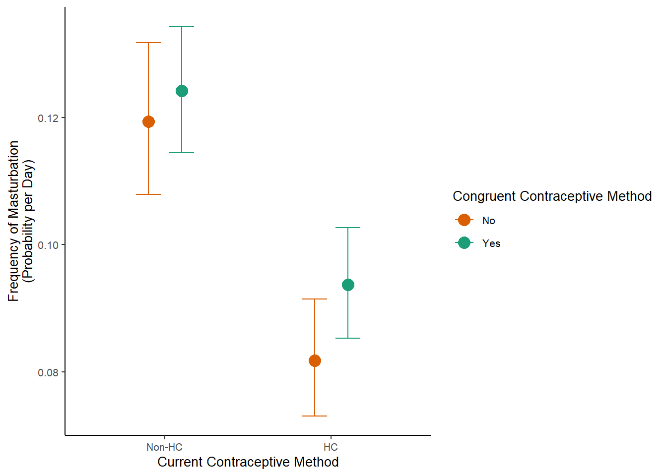

Combine Plots

congruency_controlled =
  ggarrange(m_congruency_atrr_controlled_plot + rremove("xlab"),
            m_congruency_relsat_controlled_plot + rremove("xlab"),
          m_congruency_sexsat_controlled_plot + rremove("xlab"),
          m_congruency_libido_controlled_plot + rremove("xlab"),
          m_congruency_sexfreqpen_controlled_plot,
          m_congruency_masfreq_controlled_plot,
          common.legend = TRUE, legend = "bottom",
          ncol = 2, nrow = 3,
          align = "v")

congruency_controlled

jpeg('Differences in current contraceptive method, congruent use of contraceptive method, and their interaction in controlled models.jpg', 
     width = 800, height = 1000, quality = 100)
congruency_controlled
dev.off()

## png 
##   2