Analyses Effects of Contraception
Effects of Hormonal Contraceptives
Attractiveness of Partner
Model
Summary
##  Family: gaussian
##   Links: mu = identity; sigma = identity
## Formula: attractiveness_partner ~ contraception_hormonal
##    Data: data (Number of observations: 774)
##   Draws: 4 chains, each with iter = 2000; warmup = 1000; thin = 1;
##          total post-warmup draws = 4000
##
## Population-Level Effects:
##                           Estimate Est.Error l-90% CI u-90% CI Rhat Bulk_ESS Tail_ESS
## Intercept                     4.21      0.04     4.15     4.27 1.00     3926     2990
## contraception_hormonalyes     0.08      0.05    -0.00     0.17 1.00     3780     2987
##
## Family Specific Parameters:
##       Estimate Est.Error l-90% CI u-90% CI Rhat Bulk_ESS Tail_ESS
## sigma     0.74      0.02     0.71     0.77 1.00     4114     2621
##
## Draws were sampled using sampling(NUTS). For each parameter, Bulk_ESS
## and Tail_ESS are effective sample size measures, and Rhat is the potential
## scale reduction factor on split chains (at convergence, Rhat = 1).
Comparison with ROPE
## Picking joint bandwidth of 0.00731## Warning: Removed 399 rows containing non-finite values (stat_density_ridges).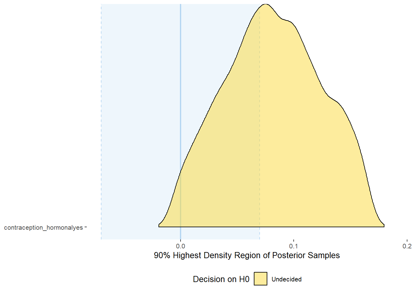
## # A tibble: 1 x 10
##   Parameter         CI ROPE_low ROPE_high ROPE_Percentage ROPE_Equivalence  HDI_low HDI_high Effects Component
##   <chr>          <dbl>    <dbl>     <dbl>           <dbl> <chr>               <dbl>    <dbl> <chr>   <chr>
## 1 b_contracepti~   0.9    -0.07      0.07           0.400 Undecided        -0.00626    0.166 fixed   conditio~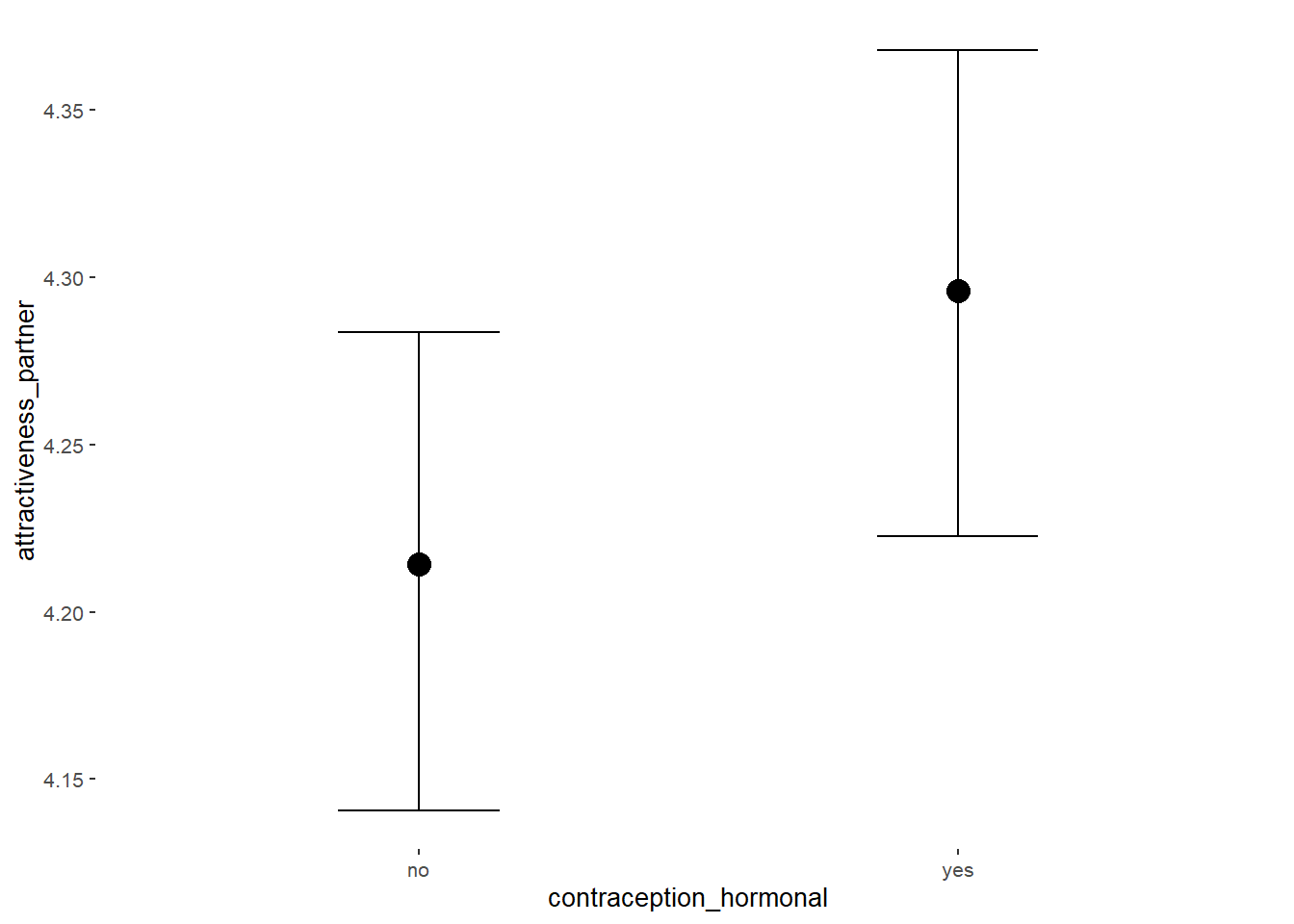
Forest Plot for Effect Sizes
m_hc_atrr %>%
  spread_draws(b_contraception_hormonalyes) %>%
  pivot_longer(cols = c(b_contraception_hormonalyes),
               names_to = "condition",
               values_to = "r_condition") %>%
  mutate(condition_mean = r_condition,
         group = ifelse(condition %contains% "b_contraception_hormonalyes",
                        "Contraception", NA),
         condition = ifelse(condition %contains% "b_contraception_hormonalyes",
                        "Hormonal Contraception", NA)) %>%
  ggplot(aes(y = condition,
             x = condition_mean,
             fill = stat(abs(x) < 0.07))) +
  stat_halfeye() +
  geom_vline(xintercept = c(-0.07, 0.07), linetype = "dotted") +
  apatheme +
  theme(legend.position = "none") +
  scale_fill_manual(values = c("gray80", "skyblue")) +
  labs(x = "Effect Size Estimates", y = "Predictors") +
  xlim (-0.6, 0.6)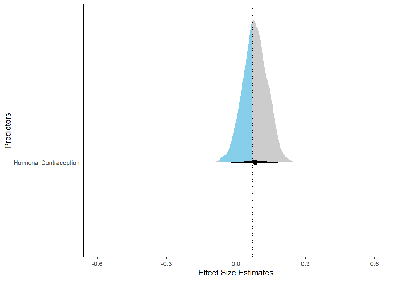
Relationship Satisfaction
Model
Summary
##  Family: gaussian
##   Links: mu = identity; sigma = identity
## Formula: relationship_satisfaction ~ contraception_hormonal
##    Data: data (Number of observations: 774)
##   Draws: 4 chains, each with iter = 2000; warmup = 1000; thin = 1;
##          total post-warmup draws = 4000
##
## Population-Level Effects:
##                           Estimate Est.Error l-90% CI u-90% CI Rhat Bulk_ESS Tail_ESS
## Intercept                     3.35      0.02     3.32     3.39 1.00     4070     2976
## contraception_hormonalyes     0.08      0.03     0.03     0.14 1.00     4119     2869
##
## Family Specific Parameters:
##       Estimate Est.Error l-90% CI u-90% CI Rhat Bulk_ESS Tail_ESS
## sigma     0.42      0.01     0.41     0.44 1.00     4602     2782
##
## Draws were sampled using sampling(NUTS). For each parameter, Bulk_ESS
## and Tail_ESS are effective sample size measures, and Rhat is the potential
## scale reduction factor on split chains (at convergence, Rhat = 1).
Comparison with ROPE
plot(equivalence_test(m_hc_relsat, range = c(-0.04, 0.04), ci = 0.90,
                      parameters = "contraception"))
## Picking joint bandwidth of 0.00438## Warning: Removed 399 rows containing non-finite values (stat_density_ridges).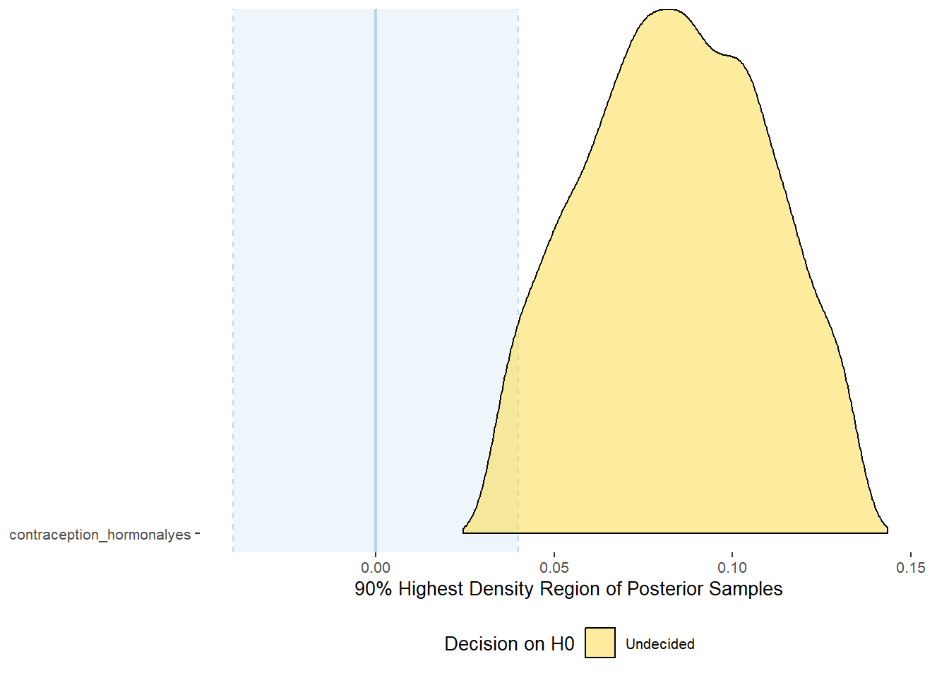
## # A tibble: 1 x 10
##   Parameter          CI ROPE_low ROPE_high ROPE_Percentage ROPE_Equivalence HDI_low HDI_high Effects Component
##   <chr>           <dbl>    <dbl>     <dbl>           <dbl> <chr>              <dbl>    <dbl> <chr>   <chr>
## 1 b_contraceptio~   0.9    -0.04      0.04          0.0361 Undecided         0.0325    0.135 fixed   conditio~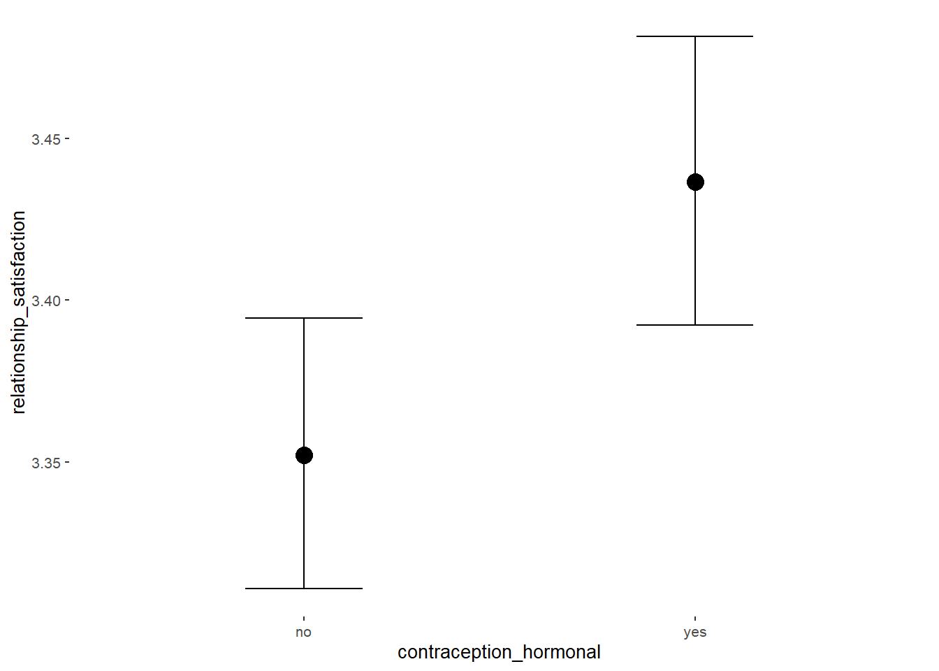
Forest Plot for Effect Sizes
m_hc_relsat %>%
  spread_draws(b_contraception_hormonalyes) %>%
  pivot_longer(cols = c(b_contraception_hormonalyes),
               names_to = "condition",
               values_to = "r_condition") %>%
  mutate(condition_mean = r_condition,
         group = ifelse(condition %contains% "b_contraception_hormonalyes",
                        "Contraception", NA),
         condition = ifelse(condition %contains% "b_contraception_hormonalyes",
                        "Hormonal Contraception", NA)) %>%
  ggplot(aes(y = condition,
             x = condition_mean,
             fill = stat(abs(x) < 0.04))) +
  stat_halfeye() +
  geom_vline(xintercept = c(-0.04, 0.04), linetype = "dotted") +
  apatheme +
  theme(legend.position = "none") +
  scale_fill_manual(values = c("gray80", "skyblue")) +
  labs(x = "Effect Size Estimates", y = "Predictors") +
  xlim (-0.6, 0.6)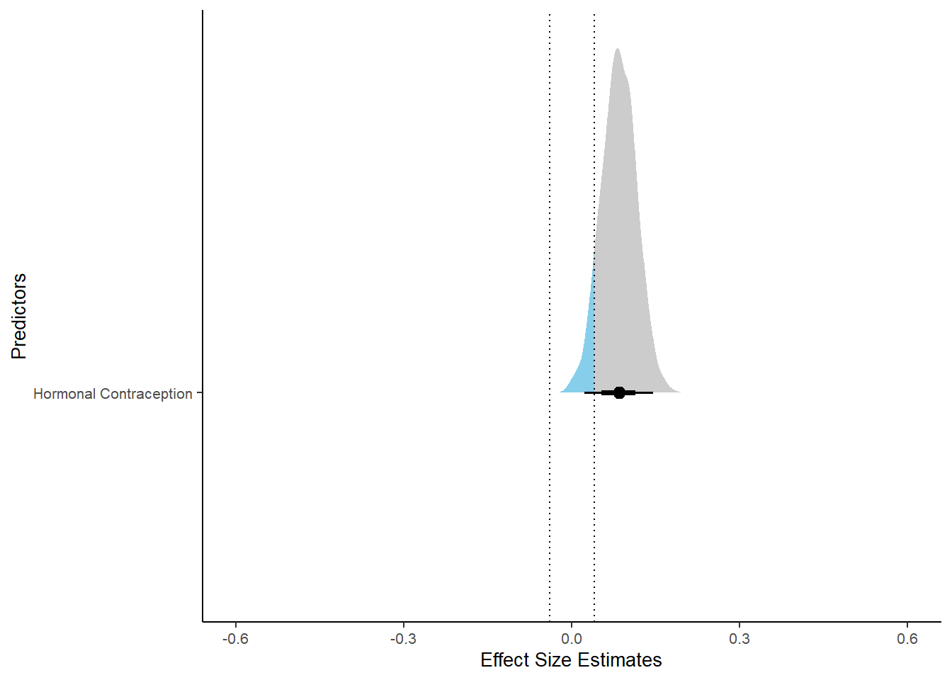
Sexual Satisfaction
Model
Summary
##  Family: gaussian
##   Links: mu = identity; sigma = identity
## Formula: satisfaction_sexual_intercourse ~ contraception_hormonal
##    Data: data (Number of observations: 774)
##   Draws: 4 chains, each with iter = 2000; warmup = 1000; thin = 1;
##          total post-warmup draws = 4000
##
## Population-Level Effects:
##                           Estimate Est.Error l-90% CI u-90% CI Rhat Bulk_ESS Tail_ESS
## Intercept                     3.94      0.05     3.84     4.03 1.00     4000     2867
## contraception_hormonalyes     0.14      0.08     0.01     0.26 1.00     4133     3129
##
## Family Specific Parameters:
##       Estimate Est.Error l-90% CI u-90% CI Rhat Bulk_ESS Tail_ESS
## sigma     1.05      0.03     1.01     1.10 1.00     4281     2820
##
## Draws were sampled using sampling(NUTS). For each parameter, Bulk_ESS
## and Tail_ESS are effective sample size measures, and Rhat is the potential
## scale reduction factor on split chains (at convergence, Rhat = 1).
Comparison with ROPE
plot(equivalence_test(m_hc_sexsat, range = c(-0.11, 0.11), ci = 0.90,
                      parameters = "contraception"))
## Picking joint bandwidth of 0.0106## Warning: Removed 399 rows containing non-finite values (stat_density_ridges).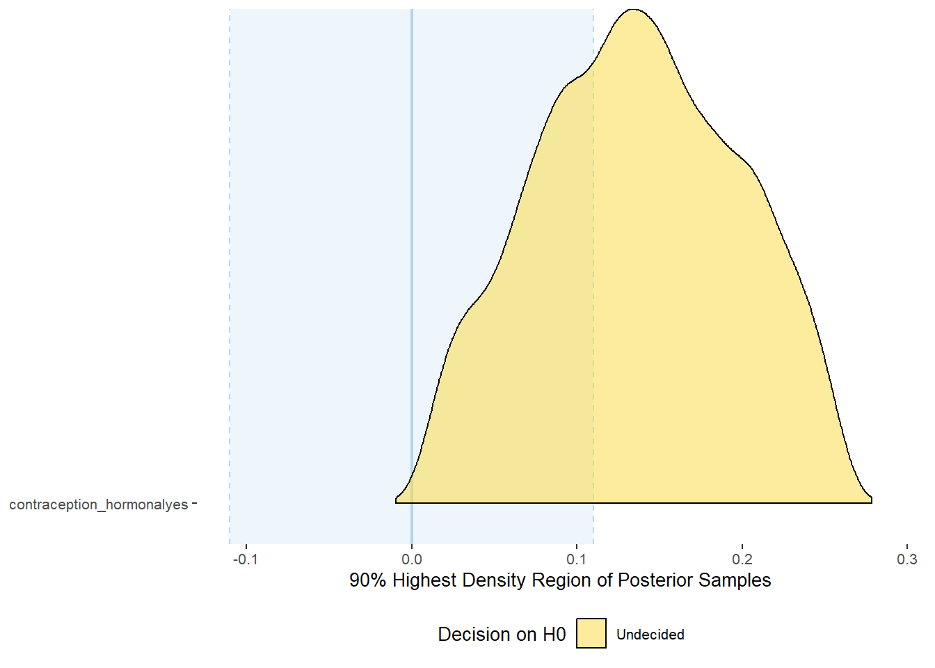
## # A tibble: 1 x 10
##   Parameter          CI ROPE_low ROPE_high ROPE_Percentage ROPE_Equivalence HDI_low HDI_high Effects Component
##   <chr>           <dbl>    <dbl>     <dbl>           <dbl> <chr>              <dbl>    <dbl> <chr>   <chr>
## 1 b_contraceptio~   0.9    -0.11      0.11           0.347 Undecided        0.00914    0.259 fixed   conditio~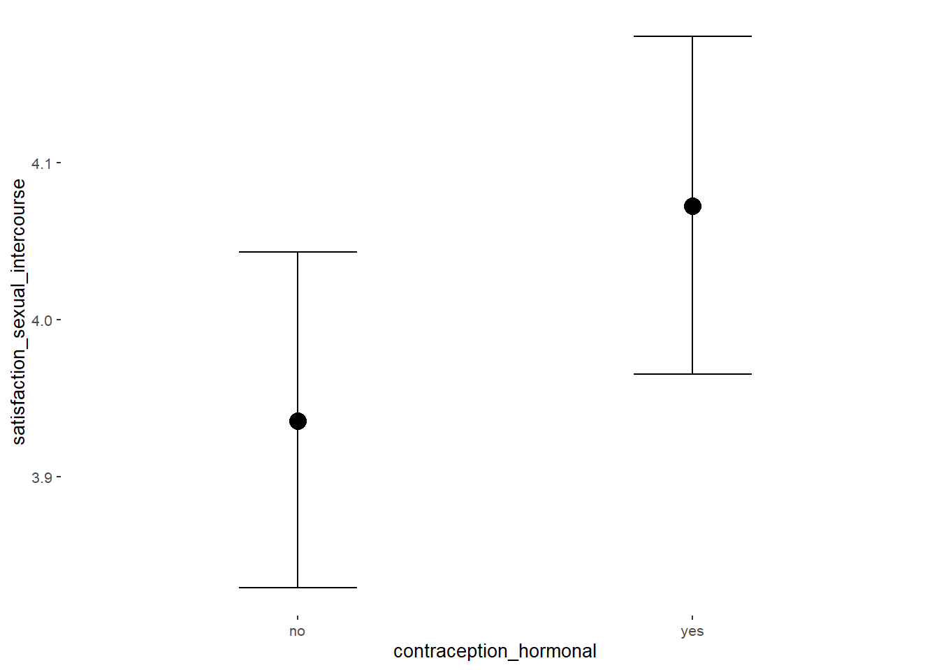
Forest Plot for Effect Sizes
m_hc_sexsat %>%
  spread_draws(b_contraception_hormonalyes) %>%
  pivot_longer(cols = c(b_contraception_hormonalyes),
               names_to = "condition",
               values_to = "r_condition") %>%
  mutate(condition_mean = r_condition,
         group = ifelse(condition %contains% "b_contraception_hormonalyes",
                        "Contraception", NA),
         condition = ifelse(condition %contains% "b_contraception_hormonalyes",
                        "Hormonal Contraception", NA)) %>%
  ggplot(aes(y = condition,
             x = condition_mean,
             fill = stat(abs(x) < 0.11))) +
  stat_halfeye() +
  geom_vline(xintercept = c(-0.11, 0.11), linetype = "dotted") +
  apatheme +
  theme(legend.position = "none") +
  scale_fill_manual(values = c("gray80", "skyblue")) +
  labs(x = "Effect Size Estimates", y = "Predictors") +
  xlim (-0.6, 0.6)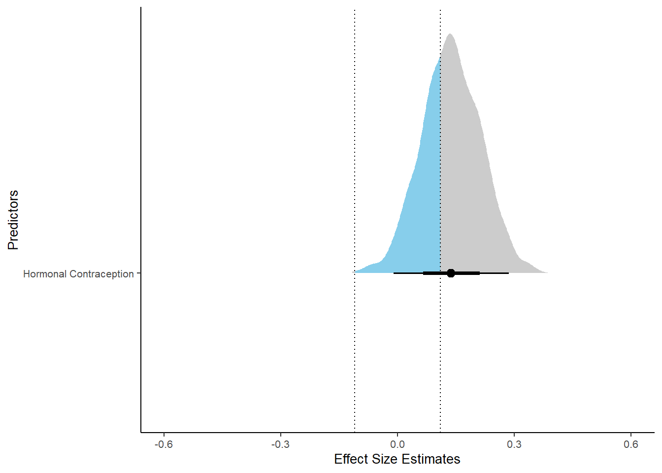
Libido
Model
Summary
## Family: gaussian
## Links: mu = identity; sigma = identity
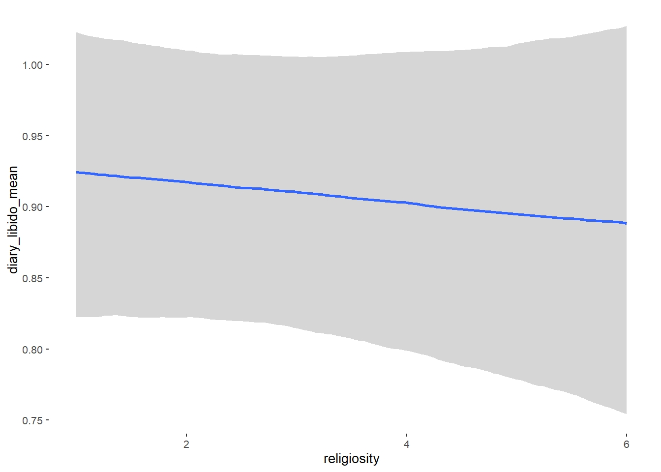
## Formula: diary_libido_mean ~ contraception_hormonal
## Data: data (Number of observations: 968)
## Draws: 4 chains, each with iter = 2000; warmup = 1000; thin = 1;
## total post-warmup draws = 4000
##
## Population-Level Effects:
## Estimate Est.Error l-90% CI u-90% CI Rhat Bulk_ESS Tail_ESS
## Intercept 1.18 0.02 1.14 1.22 1.00 4104 3097
## contraception_hormonalyes 0.02 0.04 -0.04 0.08 1.00 4305 2788
##
## Family Specific Parameters:
## Estimate Est.Error l-90% CI u-90% CI Rhat Bulk_ESS Tail_ESS
## sigma 0.59 0.01 0.57 0.61 1.00 3347 2731
##
## Draws were sampled using sampling(NUTS). For each parameter, Bulk_ESS
## and Tail_ESS are effective sample size measures, and Rhat is the potential
## scale reduction factor on split chains (at convergence, Rhat = 1).Comparison with ROPE
plot(equivalence_test(m_hc_libido, range = c(-0.06, 0.06), ci = 0.90,
                      parameters = "contraception"))
## Picking joint bandwidth of 0.00544## Warning: Removed 399 rows containing non-finite values (stat_density_ridges).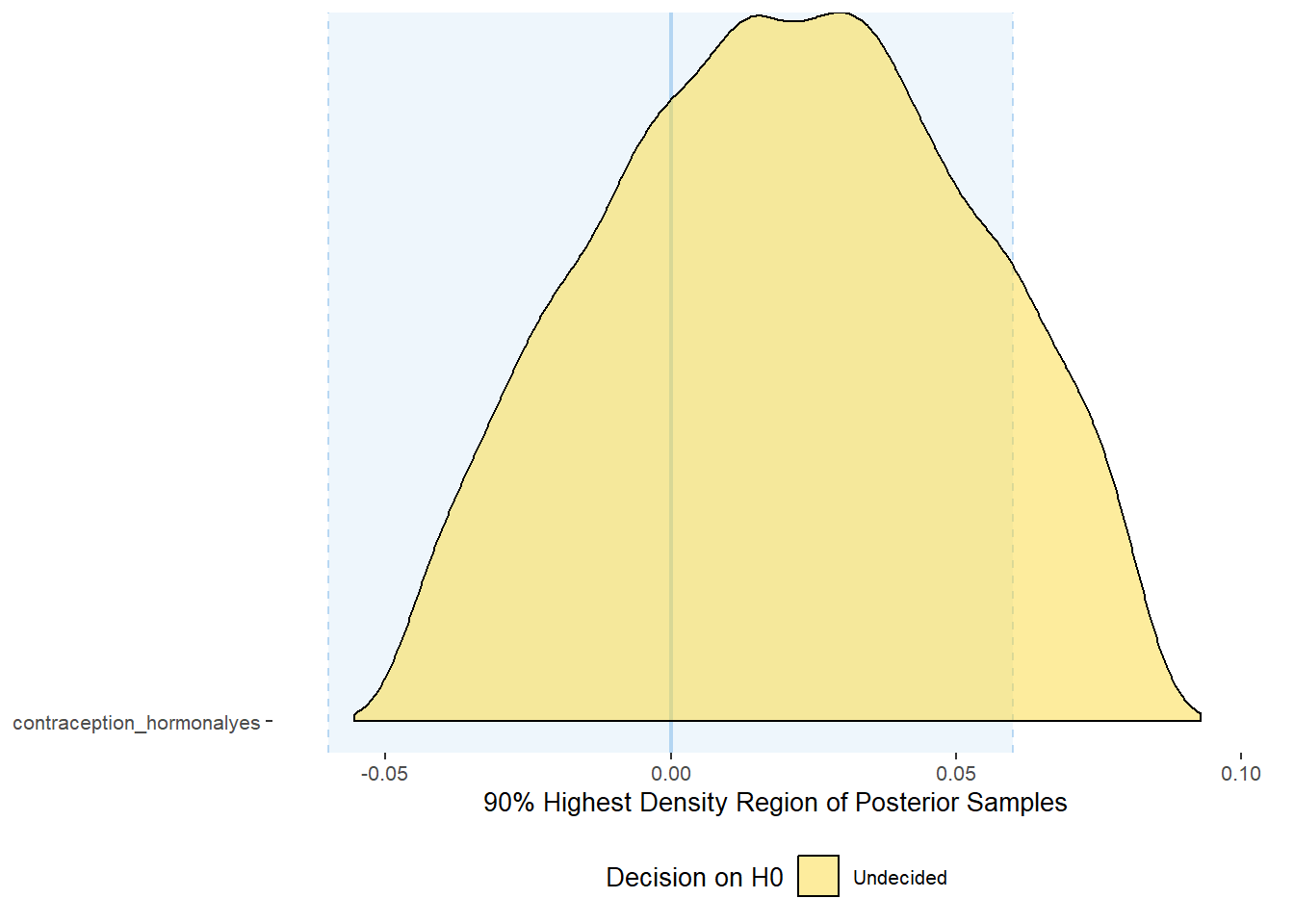
## # A tibble: 1 x 10
##   Parameter          CI ROPE_low ROPE_high ROPE_Percentage ROPE_Equivalence HDI_low HDI_high Effects Component
##   <chr>           <dbl>    <dbl>     <dbl>           <dbl> <chr>              <dbl>    <dbl> <chr>   <chr>
## 1 b_contraceptio~   0.9    -0.06      0.06           0.884 Undecided        -0.0455   0.0826 fixed   conditio~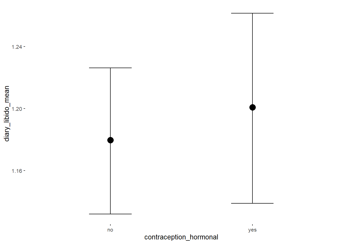
Forest Plot for Effect Sizes
m_hc_libido %>%
  spread_draws(b_contraception_hormonalyes) %>%
  pivot_longer(cols = c(b_contraception_hormonalyes),
               names_to = "condition",
               values_to = "r_condition") %>%
  mutate(condition_mean = r_condition,
         group = ifelse(condition %contains% "b_contraception_hormonalyes",
                        "Contraception", NA),
         condition = ifelse(condition %contains% "b_contraception_hormonalyes",
                        "Hormonal Contraception", NA)) %>%
  ggplot(aes(y = condition,
             x = condition_mean,
             fill = stat(abs(x) < 0.06))) +
  stat_halfeye() +
  geom_vline(xintercept = c(-0.06, 0.06), linetype = "dotted") +
  apatheme +
  theme(legend.position = "none") +
  scale_fill_manual(values = c("gray80", "skyblue")) +
  labs(x = "Effect Size Estimates", y = "Predictors") +
  xlim (-0.6, 0.6)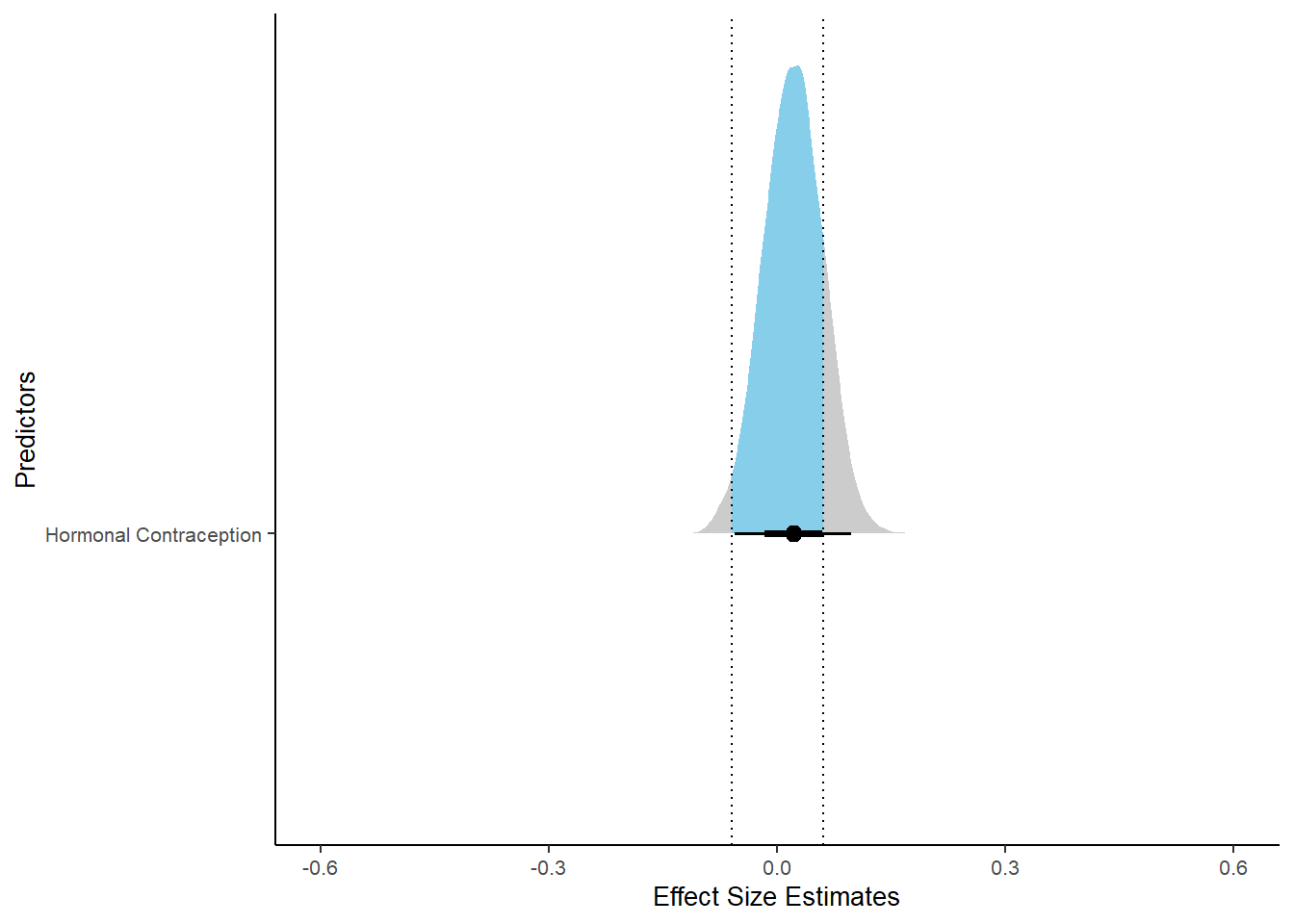
Sexual Frequency (Penetrative Intercourse)
Model
Summary
##  Family: poisson
##   Links: mu = log
## Formula: diary_sex_active_sex_sum ~ offset(log(number_of_days)) + contraception_hormonal
##    Data: data (Number of observations: 897)
##   Draws: 4 chains, each with iter = 2000; warmup = 1000; thin = 1;
##          total post-warmup draws = 4000
##
## Population-Level Effects:
##                           Estimate Est.Error l-90% CI u-90% CI Rhat Bulk_ESS Tail_ESS
## Intercept                    -2.09      0.02    -2.12    -2.06 1.00     3349     2343
## contraception_hormonalyes     0.25      0.03     0.21     0.29 1.00     3880     2592
##
## Draws were sampled using sampling(NUTS). For each parameter, Bulk_ESS
## and Tail_ESS are effective sample size measures, and Rhat is the potential
## scale reduction factor on split chains (at convergence, Rhat = 1).
Comparison with ROPE
plot(equivalence_test(m_hc_sexfreqpen, range = c(-0.05, 0.05)), ci = 0.90,
                      parameters = "contraception")
## Picking joint bandwidth of 0.00387## Warning: Removed 199 rows containing non-finite values (stat_density_ridges).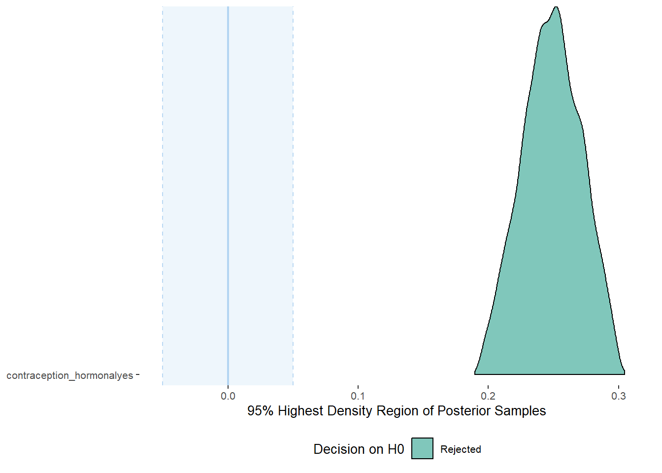
## # A tibble: 1 x 10
##   Parameter          CI ROPE_low ROPE_high ROPE_Percentage ROPE_Equivalence HDI_low HDI_high Effects Component
##   <chr>           <dbl>    <dbl>     <dbl>           <dbl> <chr>              <dbl>    <dbl> <chr>   <chr>
## 1 b_contraceptio~   0.9    -0.05      0.05               0 Rejected           0.205    0.290 fixed   conditio~
Plots
conditional_effects(m_hc_sexfreqpen,
                    effects = "contraception_hormonal",
                    conditions = data.frame(number_of_days = 1))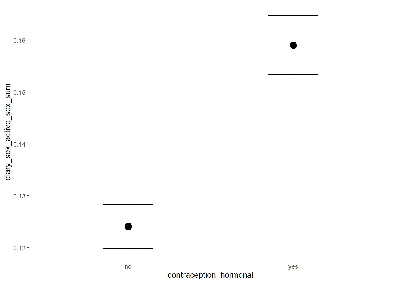
Forest Plot for Effect Sizes
m_hc_sexfreqpen %>%
  spread_draws(b_contraception_hormonalyes) %>%
  pivot_longer(cols = c(b_contraception_hormonalyes),
               names_to = "condition",
               values_to = "r_condition") %>%
  mutate(condition_mean = r_condition,
         group = ifelse(condition %contains% "b_contraception_hormonalyes",
                        "Contraception", NA),
         condition = ifelse(condition %contains% "b_contraception_hormonalyes",
                        "Hormonal Contraception", NA)) %>%
  ggplot(aes(y = condition,
             x = condition_mean,
             fill = stat(abs(x) < 0.05))) +
  stat_halfeye() +
  geom_vline(xintercept = c(-0.05, 0.05), linetype = "dotted") +
  apatheme +
  theme(legend.position = "none") +
  scale_fill_manual(values = c("gray80", "skyblue")) +
  labs(x = "Effect Size Estimates", y = "Predictors")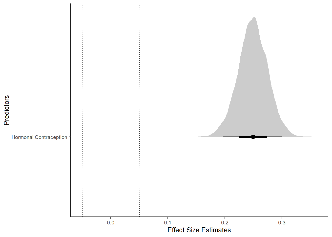
Masturbation Frequency
Model
Summary
##  Family: poisson
##   Links: mu = log
## Formula: diary_masturbation_sum ~ offset(log(number_of_days)) + contraception_hormonal
##    Data: data (Number of observations: 897)
##   Draws: 4 chains, each with iter = 2000; warmup = 1000; thin = 1;
##          total post-warmup draws = 4000
##
## Population-Level Effects:
##                           Estimate Est.Error l-90% CI u-90% CI Rhat Bulk_ESS Tail_ESS
## Intercept                    -1.88      0.02    -1.90    -1.85 1.00     4566     3063
## contraception_hormonalyes    -0.40      0.03    -0.44    -0.35 1.00     2847     2414
##
## Draws were sampled using sampling(NUTS). For each parameter, Bulk_ESS
## and Tail_ESS are effective sample size measures, and Rhat is the potential
## scale reduction factor on split chains (at convergence, Rhat = 1).
Comparison with ROPE
plot(equivalence_test(m_hc_masfreq, range = c(-0.05, 0.05), ci = 0.90,
                      parameters = "contraception"))
## Picking joint bandwidth of 0.00367## Warning: Removed 399 rows containing non-finite values (stat_density_ridges).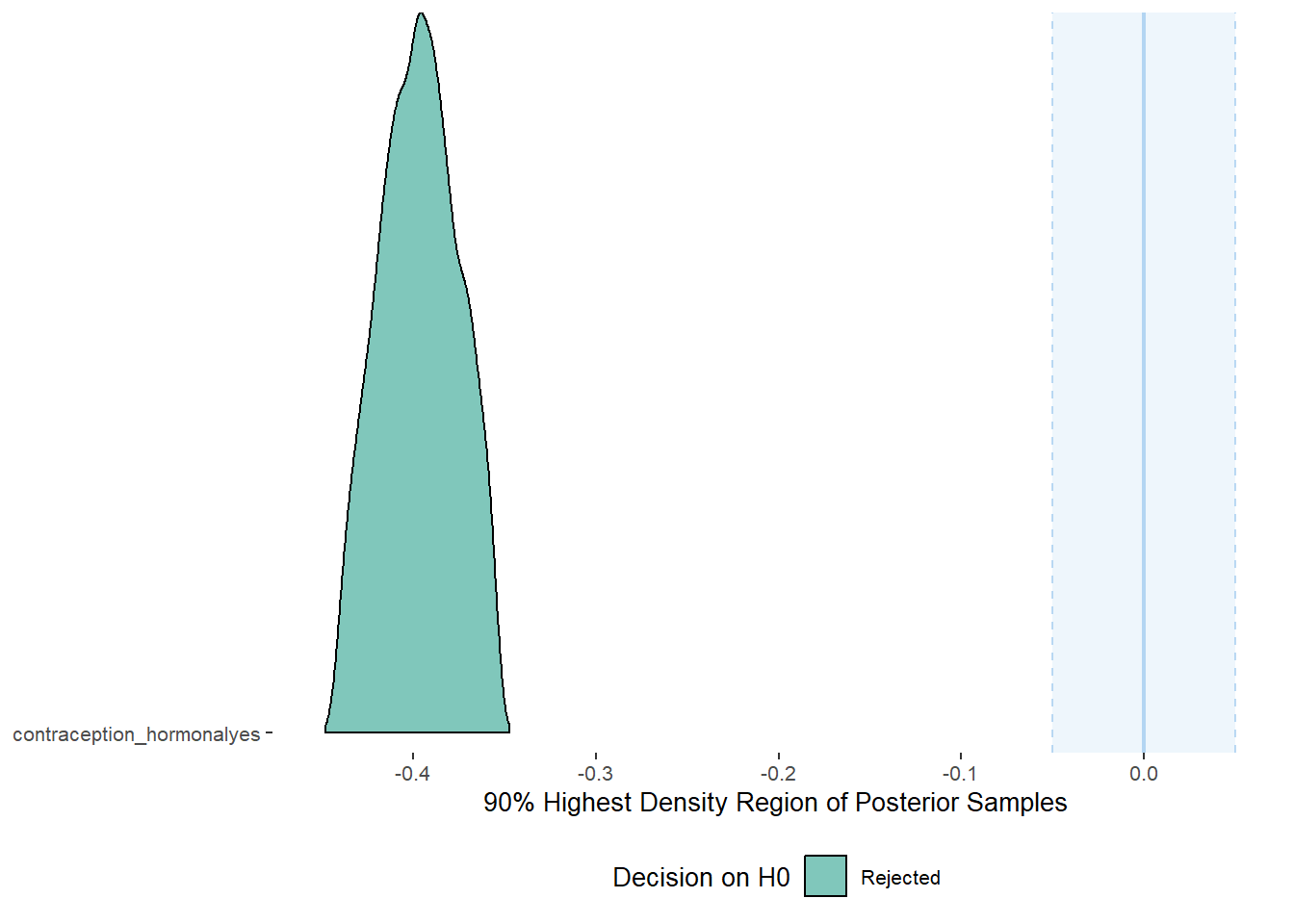
## # A tibble: 1 x 10
##   Parameter          CI ROPE_low ROPE_high ROPE_Percentage ROPE_Equivalence HDI_low HDI_high Effects Component
##   <chr>           <dbl>    <dbl>     <dbl>           <dbl> <chr>              <dbl>    <dbl> <chr>   <chr>
## 1 b_contraceptio~   0.9    -0.05      0.05               0 Rejected          -0.441   -0.354 fixed   conditio~
Plots
conditional_effects(m_hc_masfreq,
                    effects = "contraception_hormonal",
                    conditions = data.frame(number_of_days = 1))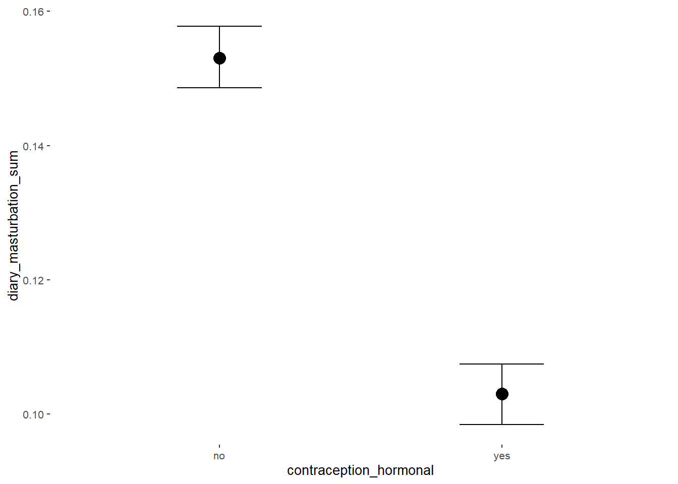
Forest Plot for Effect Sizes
m_hc_masfreq %>%
  spread_draws(b_contraception_hormonalyes) %>%
  pivot_longer(cols = c(b_contraception_hormonalyes),
               names_to = "condition",
               values_to = "r_condition") %>%
  mutate(condition_mean = r_condition,
         group = ifelse(condition %contains% "b_contraception_hormonalyes",
                        "Contraception", NA),
         condition = ifelse(condition %contains% "b_contraception_hormonalyes",
                        "Hormonal Contraception", NA)) %>%
  ggplot(aes(y = condition,
             x = condition_mean,
             fill = stat(abs(x) < 0.05))) +
  stat_halfeye() +
  geom_vline(xintercept = c(-0.05, 0.05), linetype = "dotted") +
  apatheme +
  theme(legend.position = "none") +
  scale_fill_manual(values = c("gray80", "skyblue")) +
  labs(x = "Effect Size Estimates", y = "Predictors")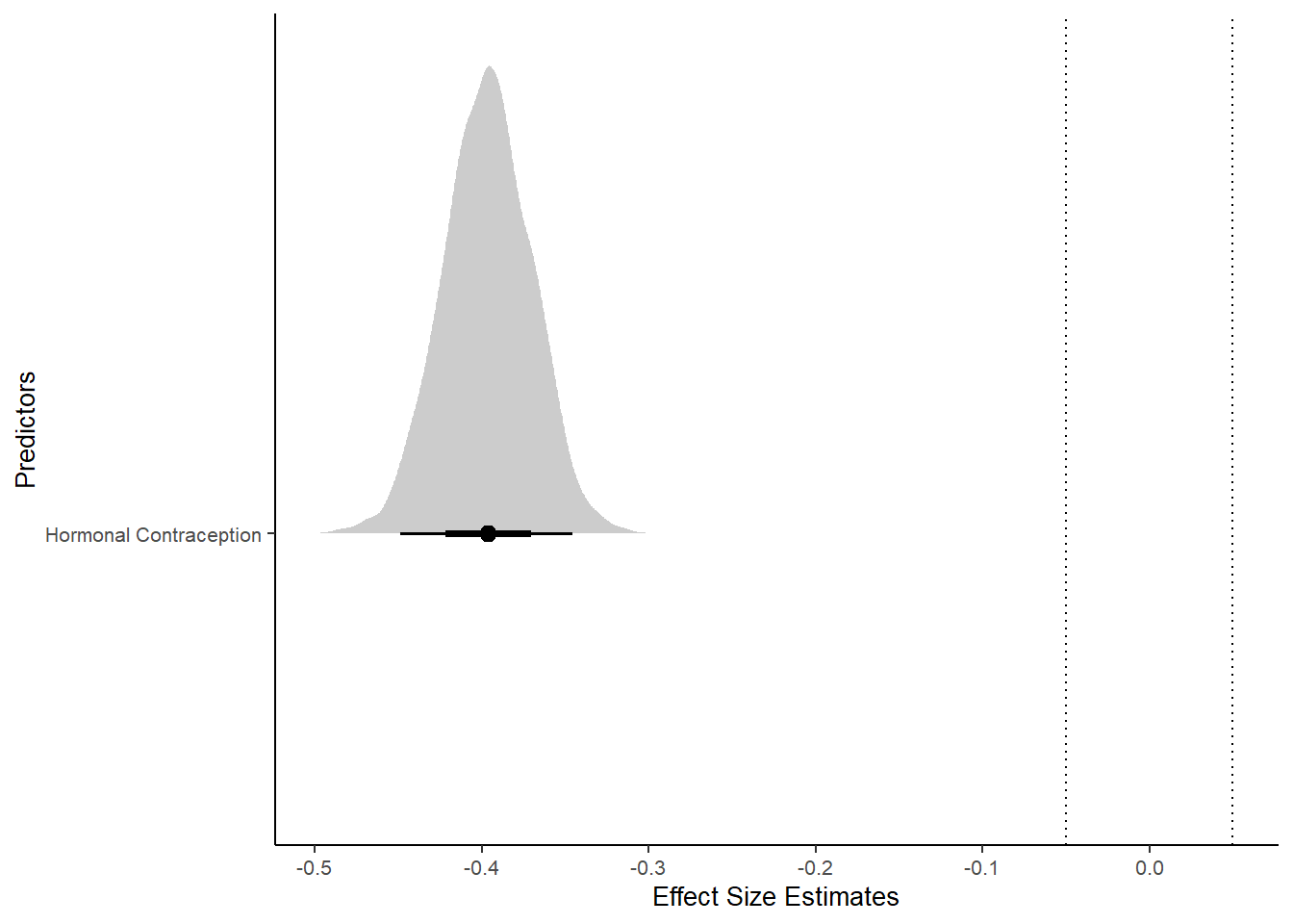
Controlled Models: Effects of Hormonal Contraceptives
Attractiveness of Partner
Model
m_hc_atrr_controlled = brm(attractiveness_partner ~ contraception_hormonal +
                             age + net_income + relationship_duration_factor +
                              education_years +
                              bfi_extra + bfi_neuro + bfi_agree + bfi_consc + bfi_open +
                              religiosity,
                data = data, family = gaussian(),
                file = "m_hc_atrr_controlled")
## Warning: Rows containing NAs were excluded from the model.## Compiling Stan program...## Start sampling##
## SAMPLING FOR MODEL 'e2eceadeaf05fc7906f2a27d8d9a066f' NOW (CHAIN 1).
## Chain 1:
## Chain 1: Gradient evaluation took 0 seconds
## Chain 1: 1000 transitions using 10 leapfrog steps per transition would take 0 seconds.
## Chain 1: Adjust your expectations accordingly!
## Chain 1:
## Chain 1:
## Chain 1: Iteration: 1 / 2000 [ 0%] (Warmup)
## Chain 1: Iteration: 200 / 2000 [ 10%] (Warmup)
## Chain 1: Iteration: 400 / 2000 [ 20%] (Warmup)
## Chain 1: Iteration: 600 / 2000 [ 30%] (Warmup)
## Chain 1: Iteration: 800 / 2000 [ 40%] (Warmup)
## Chain 1: Iteration: 1000 / 2000 [ 50%] (Warmup)
## Chain 1: Iteration: 1001 / 2000 [ 50%] (Sampling)
## Chain 1: Iteration: 1200 / 2000 [ 60%] (Sampling)
## Chain 1: Iteration: 1400 / 2000 [ 70%] (Sampling)
## Chain 1: Iteration: 1600 / 2000 [ 80%] (Sampling)
## Chain 1: Iteration: 1800 / 2000 [ 90%] (Sampling)
## Chain 1: Iteration: 2000 / 2000 [100%] (Sampling)
## Chain 1:
## Chain 1: Elapsed Time: 10.787 seconds (Warm-up)
## Chain 1: 12.406 seconds (Sampling)
## Chain 1: 23.193 seconds (Total)
## Chain 1:
##
## SAMPLING FOR MODEL 'e2eceadeaf05fc7906f2a27d8d9a066f' NOW (CHAIN 2).
## Chain 2:
## Chain 2: Gradient evaluation took 0 seconds
## Chain 2: 1000 transitions using 10 leapfrog steps per transition would take 0 seconds.
## Chain 2: Adjust your expectations accordingly!
## Chain 2:
## Chain 2:
## Chain 2: Iteration: 1 / 2000 [ 0%] (Warmup)
## Chain 2: Iteration: 200 / 2000 [ 10%] (Warmup)
## Chain 2: Iteration: 400 / 2000 [ 20%] (Warmup)
## Chain 2: Iteration: 600 / 2000 [ 30%] (Warmup)
## Chain 2: Iteration: 800 / 2000 [ 40%] (Warmup)
## Chain 2: Iteration: 1000 / 2000 [ 50%] (Warmup)
## Chain 2: Iteration: 1001 / 2000 [ 50%] (Sampling)
## Chain 2: Iteration: 1200 / 2000 [ 60%] (Sampling)
## Chain 2: Iteration: 1400 / 2000 [ 70%] (Sampling)
## Chain 2: Iteration: 1600 / 2000 [ 80%] (Sampling)
## Chain 2: Iteration: 1800 / 2000 [ 90%] (Sampling)
## Chain 2: Iteration: 2000 / 2000 [100%] (Sampling)
## Chain 2:
## Chain 2: Elapsed Time: 10.786 seconds (Warm-up)
## Chain 2: 12.547 seconds (Sampling)
## Chain 2: 23.333 seconds (Total)
## Chain 2:
##
## SAMPLING FOR MODEL 'e2eceadeaf05fc7906f2a27d8d9a066f' NOW (CHAIN 3).
## Chain 3:
## Chain 3: Gradient evaluation took 0 seconds
## Chain 3: 1000 transitions using 10 leapfrog steps per transition would take 0 seconds.
## Chain 3: Adjust your expectations accordingly!
## Chain 3:
## Chain 3:
## Chain 3: Iteration: 1 / 2000 [ 0%] (Warmup)
## Chain 3: Iteration: 200 / 2000 [ 10%] (Warmup)
## Chain 3: Iteration: 400 / 2000 [ 20%] (Warmup)
## Chain 3: Iteration: 600 / 2000 [ 30%] (Warmup)
## Chain 3: Iteration: 800 / 2000 [ 40%] (Warmup)
## Chain 3: Iteration: 1000 / 2000 [ 50%] (Warmup)
## Chain 3: Iteration: 1001 / 2000 [ 50%] (Sampling)
## Chain 3: Iteration: 1200 / 2000 [ 60%] (Sampling)
## Chain 3: Iteration: 1400 / 2000 [ 70%] (Sampling)
## Chain 3: Iteration: 1600 / 2000 [ 80%] (Sampling)
## Chain 3: Iteration: 1800 / 2000 [ 90%] (Sampling)
## Chain 3: Iteration: 2000 / 2000 [100%] (Sampling)
## Chain 3:
## Chain 3: Elapsed Time: 10.674 seconds (Warm-up)
## Chain 3: 12.357 seconds (Sampling)
## Chain 3: 23.031 seconds (Total)
## Chain 3:
##
## SAMPLING FOR MODEL 'e2eceadeaf05fc7906f2a27d8d9a066f' NOW (CHAIN 4).
## Chain 4:
## Chain 4: Gradient evaluation took 0 seconds
## Chain 4: 1000 transitions using 10 leapfrog steps per transition would take 0 seconds.
## Chain 4: Adjust your expectations accordingly!
## Chain 4:
## Chain 4:
## Chain 4: Iteration: 1 / 2000 [ 0%] (Warmup)
## Chain 4: Iteration: 200 / 2000 [ 10%] (Warmup)
## Chain 4: Iteration: 400 / 2000 [ 20%] (Warmup)
## Chain 4: Iteration: 600 / 2000 [ 30%] (Warmup)
## Chain 4: Iteration: 800 / 2000 [ 40%] (Warmup)
## Chain 4: Iteration: 1000 / 2000 [ 50%] (Warmup)
## Chain 4: Iteration: 1001 / 2000 [ 50%] (Sampling)
## Chain 4: Iteration: 1200 / 2000 [ 60%] (Sampling)
## Chain 4: Iteration: 1400 / 2000 [ 70%] (Sampling)
## Chain 4: Iteration: 1600 / 2000 [ 80%] (Sampling)
## Chain 4: Iteration: 1800 / 2000 [ 90%] (Sampling)
## Chain 4: Iteration: 2000 / 2000 [100%] (Sampling)
## Chain 4:
## Chain 4: Elapsed Time: 10.736 seconds (Warm-up)
## Chain 4: 12.141 seconds (Sampling)
## Chain 4: 22.877 seconds (Total)
## Chain 4:## Warning: There were 4000 transitions after warmup that exceeded the maximum treedepth. Increase max_treedepth above 10. See
## http://mc-stan.org/misc/warnings.html#maximum-treedepth-exceeded## Warning: Examine the pairs() plot to diagnose sampling problems## Warning: The largest R-hat is 3.51, indicating chains have not mixed.
## Running the chains for more iterations may help. See
## http://mc-stan.org/misc/warnings.html#r-hat## Warning: Bulk Effective Samples Size (ESS) is too low, indicating posterior means and medians may be unreliable.
## Running the chains for more iterations may help. See
## http://mc-stan.org/misc/warnings.html#bulk-ess## Warning: Tail Effective Samples Size (ESS) is too low, indicating posterior variances and tail quantiles may be unreliable.
## Running the chains for more iterations may help. See
## http://mc-stan.org/misc/warnings.html#tail-essSummary
## Warning: Parts of the model have not converged (some Rhats are > 1.05). Be careful when analysing the results!
## We recommend running more iterations and/or setting stronger priors.
## Family: gaussian
## Links: mu = identity; sigma = identity
## Formula: attractiveness_partner ~ contraception_hormonal + age + net_income + relationship_duration_factor + education_years + bfi_extra + bfi_neuro + bfi_agree + bfi_consc + bfi_open + religiosity
## Data: data (Number of observations: 774)
## Draws: 4 chains, each with iter = 2000; warmup = 1000; thin = 1;
## total post-warmup draws = 4000
##
## Population-Level Effects:
## Estimate Est.Error l-90% CI u-90% CI Rhat Bulk_ESS
## Intercept 302.50 600.94 -565.96 1209.77 3.51 4
## contraception_hormonalyes 0.07 0.05 -0.02 0.14 1.09 36
## age -0.00 0.01 -0.01 0.01 1.07 62
## net_incomeeuro_500_1000 0.04 0.05 -0.04 0.13 1.06 62
## net_incomeeuro_1000_2000 0.13 0.07 0.03 0.25 1.06 58
## net_incomeeuro_2000_3000 0.18 0.11 -0.01 0.34 1.05 51
## net_incomeeuro_gt_3000 0.21 0.20 -0.13 0.56 1.04 59
## net_incomedont_tell -0.01 0.16 -0.25 0.27 1.04 78
## relationship_duration_factorPartnered_upto12months -299.19 600.90 -1206.68 569.31 3.51 4
## relationship_duration_factorPartnered_upto28months -299.08 600.90 -1206.47 569.33 3.51 4
## relationship_duration_factorPartnered_upto52months -299.24 600.90 -1206.62 569.31 3.51 4
## relationship_duration_factorPartnered_morethan52months -299.34 600.89 -1206.73 569.15 3.51 4
## education_years 0.01 0.01 -0.00 0.02 1.05 59
## bfi_extra 0.05 0.03 -0.01 0.10 1.10 38
## bfi_neuro -0.00 0.04 -0.06 0.06 1.04 61
## bfi_agree 0.09 0.05 0.02 0.17 1.15 21
## bfi_consc 0.02 0.04 -0.05 0.09 1.09 40
## bfi_open 0.07 0.04 0.01 0.14 1.09 53
## religiosity -0.00 0.02 -0.03 0.03 1.03 52
## Tail_ESS
## Intercept NA
## contraception_hormonalyes NA
## age NA
## net_incomeeuro_500_1000 NA
## net_incomeeuro_1000_2000 NA
## net_incomeeuro_2000_3000 NA
## net_incomeeuro_gt_3000 NA
## net_incomedont_tell NA
## relationship_duration_factorPartnered_upto12months NA
## relationship_duration_factorPartnered_upto28months NA
## relationship_duration_factorPartnered_upto52months NA
## relationship_duration_factorPartnered_morethan52months NA
## education_years NA
## bfi_extra NA
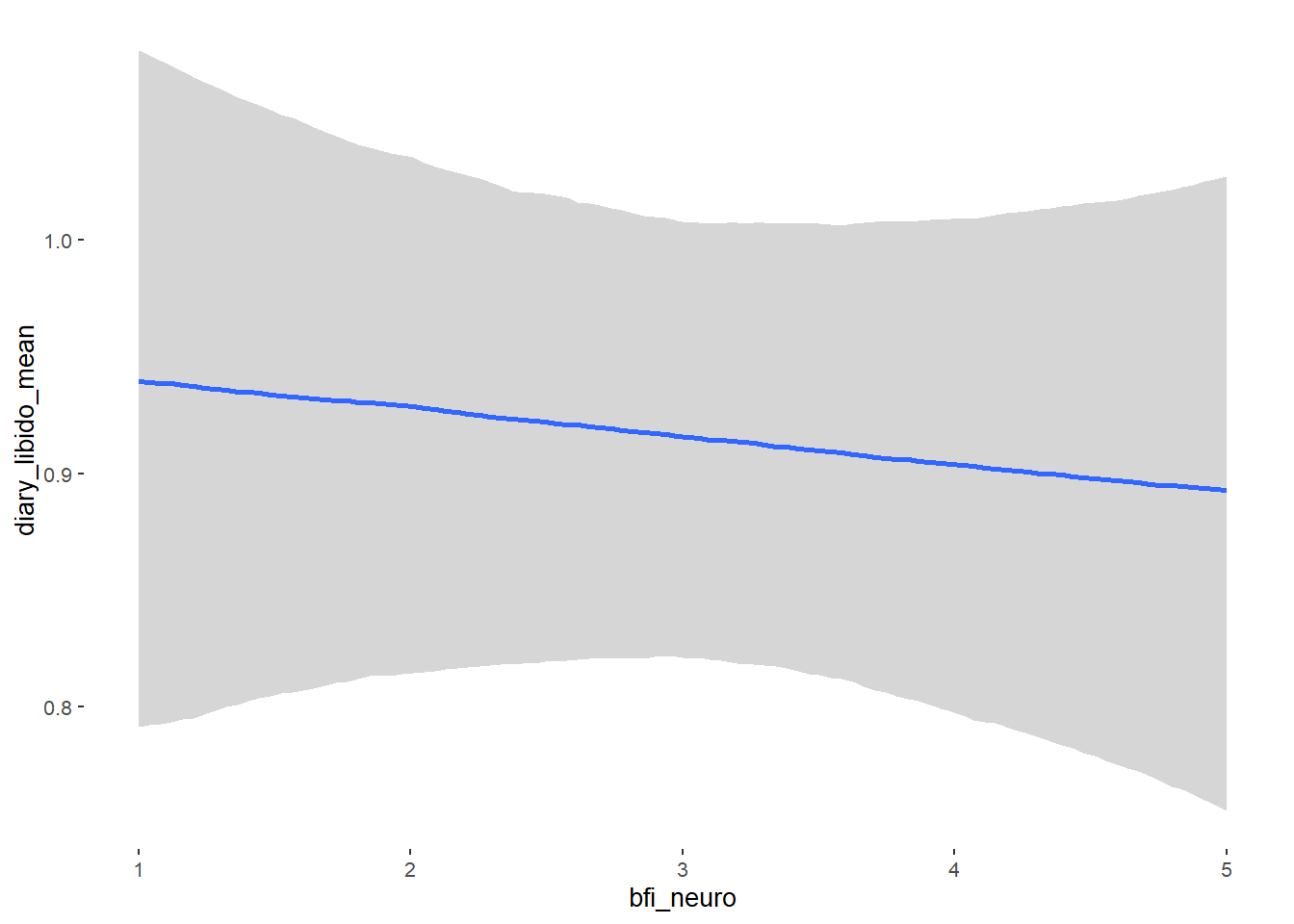
## bfi_neuro NA
## bfi_agree NA
## bfi_consc NA
## bfi_open NA
## religiosity NA
##
## Family Specific Parameters:
## Estimate Est.Error l-90% CI u-90% CI Rhat Bulk_ESS Tail_ESS
## sigma 0.73 0.02 0.69 0.76 1.22 15 NA
##
## Draws were sampled using sampling(NUTS). For each parameter, Bulk_ESS
## and Tail_ESS are effective sample size measures, and Rhat is the potential
## scale reduction factor on split chains (at convergence, Rhat = 1).Comparison with ROPE
plot(equivalence_test(m_hc_atrr_controlled, range = c(-0.07, 0.07), ci = 0.90,
                      parameters = "contraception"))
## Picking joint bandwidth of 0.00705## Warning: Removed 399 rows containing non-finite values (stat_density_ridges).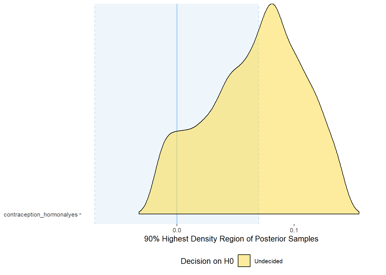
equivalence_test(m_hc_atrr_controlled, range = c(-0.07, 0.07), ci = 0.90,
                      parameters = "contraception")
## # A tibble: 1 x 10
## Parameter CI ROPE_low ROPE_high ROPE_Percentage ROPE_Equivalence HDI_low HDI_high Effects Component
## <chr> <dbl> <dbl> <dbl> <dbl> <chr> <dbl> <dbl> <chr> <chr>
## 1 b_contraceptio~ 0.9 -0.07 0.07 0.482 Undecided -0.0186 0.142 fixed conditio~
Forest Plot for Effect Sizes
m_hc_atrr_controlled %>%
spread_draws(b_contraception_hormonalyes,
b_age,
b_net_incomeeuro_500_1000, b_net_incomeeuro_1000_2000,
b_net_incomeeuro_2000_3000, b_net_incomeeuro_gt_3000, b_net_incomedont_tell,
b_relationship_duration_factorPartnered_upto28months,
b_relationship_duration_factorPartnered_upto52months,
b_relationship_duration_factorPartnered_morethan52months,
b_education_years,
b_bfi_extra, b_bfi_neuro, b_bfi_agree, b_bfi_consc, b_bfi_open,
b_religiosity) %>%
pivot_longer(cols = c(b_contraception_hormonalyes,
b_age,
b_net_incomeeuro_500_1000, b_net_incomeeuro_1000_2000,
b_net_incomeeuro_2000_3000, b_net_incomeeuro_gt_3000, b_net_incomedont_tell,
b_relationship_duration_factorPartnered_upto28months,
b_relationship_duration_factorPartnered_upto52months,
b_relationship_duration_factorPartnered_morethan52months,
b_education_years,
b_bfi_extra, b_bfi_neuro, b_bfi_agree, b_bfi_consc, b_bfi_open,
b_religiosity),
names_to = "condition",
values_to = "r_condition") %>%
mutate(condition_mean = r_condition,
group = ifelse(condition %contains% "b_relationship_duration_factor",
"Relationship Duration",
ifelse(condition %contains% "b_net_income",
"Income",
NA)),
group = ifelse(condition %contains% "b_contraception_hormonalyes",
"Contraception", group),
condition = ifelse(condition %contains% "b_contraception_hormonalyes",
"Hormonal Contraception", condition),
condition = ifelse(condition == "b_age", "Age",
ifelse(condition == "b_net_incomeeuro_500_1000", "500-1000 Euro",
ifelse(condition == "b_net_incomeeuro_1000_2000", "1000-2000 Euro",
ifelse(condition == "b_net_incomeeuro_2000_3000", "2000-3000 Euro",
ifelse(condition == "b_net_incomeeuro_gt_3000", ">3000 Euro",
ifelse(condition == "b_net_incomedont_tell", "do not tell",
ifelse(condition == "b_relationship_duration_factorPartnered_upto28months",
"13-28 months",
ifelse(condition == "b_relationship_duration_factorPartnered_upto52months",
"29-52 months",
ifelse(condition == "b_relationship_duration_factorPartnered_morethan52months",
">52 months",
ifelse(condition == "b_education_years", "Years of Education",
ifelse(condition == "b_bfi_extra", "Extraversion",
ifelse(condition == "b_bfi_neuro", "Neuroticism",
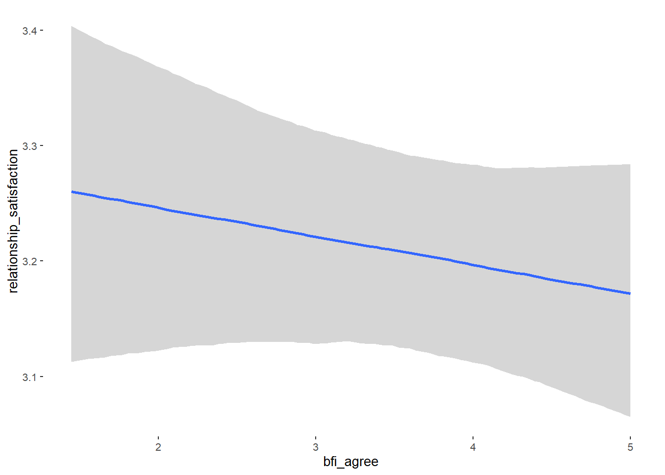
ifelse(condition == "b_bfi_agree", "Agreeableness",
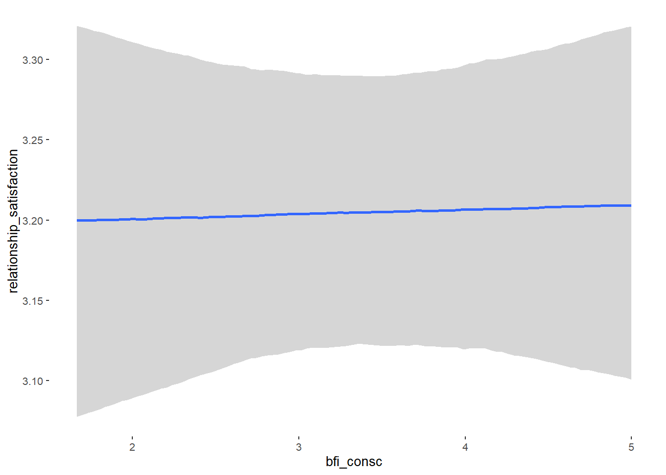
ifelse(condition == "b_bfi_consc", "Conscientiousness",
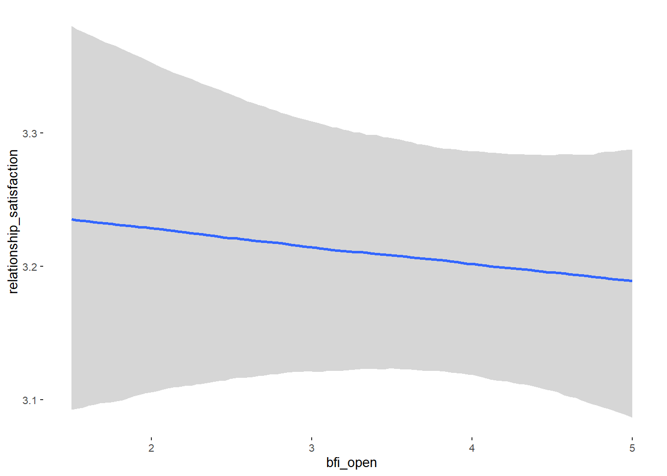
ifelse(condition == "b_bfi_open", "Openness",
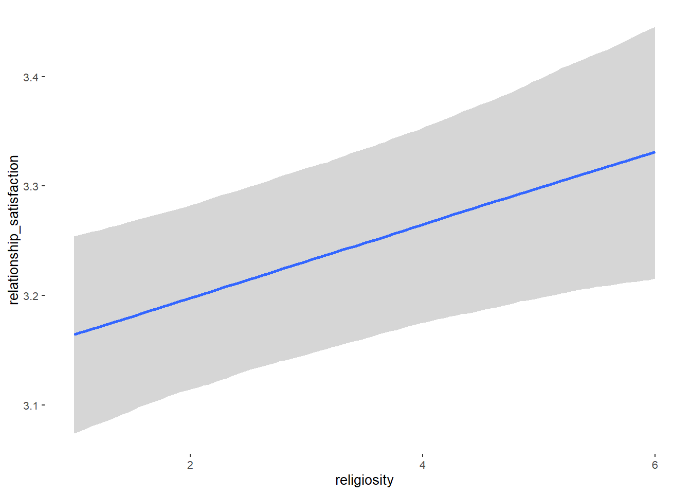
ifelse(condition == "b_religiosity", "Religiosity",
condition)))))))))))))))),
group = ifelse(is.na(group), condition, group),
condition = factor(condition, levels = rev(c("Hormonal Contraception", "Age",
"500-1000 Euro", "1000-2000 Euro",
"2000-3000 Euro", ">3000 Euro", "do not tell",
"13-28 months", "29-52 months",
">52 months",
"Years of Education",
"Extraversion", "Neuroticism", "Agreeableness",
"Conscientiousness","Openness","Religiosity"))),
group = factor(group, levels = c("Contraception", "Age", "Income",
"Relationship Duration","Years of Education",
"Extraversion", "Neuroticism", "Agreeableness",
"Conscientiousness","Openness","Religiosity"))) %>%
ggplot(aes(y = condition,
x = condition_mean,
fill = stat(abs(x) < 0.07))) +
stat_halfeye() +
geom_vline(xintercept = c(-0.07, 0.07), linetype = "dotted") +
apatheme +
theme(legend.position = "none") +
scale_fill_manual(values = c("gray80", "skyblue")) +
labs(x = "Effect Size Estimates", y = "Predictors")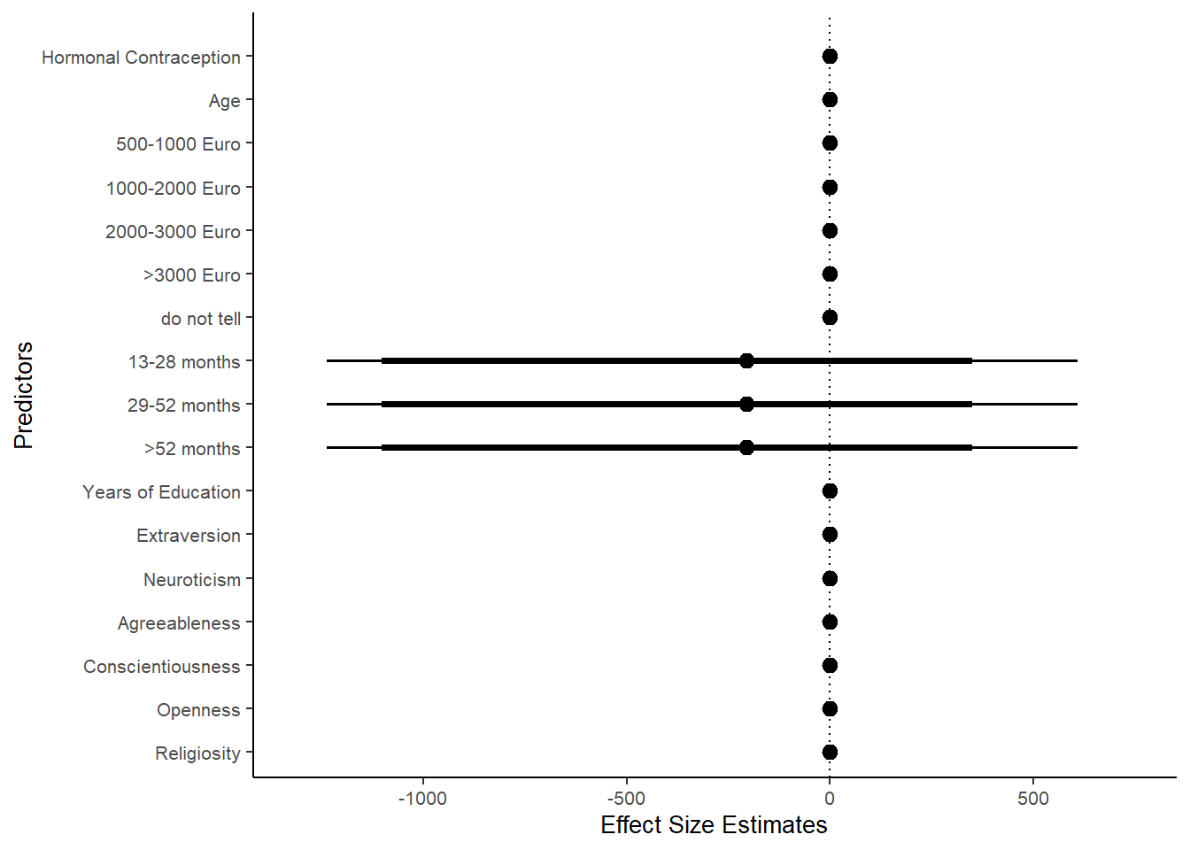
Relationship Satisfaction
Model
Summary
## Family: gaussian
## Links: mu = identity; sigma = identity
## Formula: relationship_satisfaction ~ contraception_hormonal + age + net_income + relationship_duration_factor + education_years + bfi_extra + bfi_neuro + bfi_agree + bfi_consc + bfi_open + religiosity
## Data: data (Number of observations: 774)
## Draws: 4 chains, each with iter = 2000; warmup = 1000; thin = 1;
## total post-warmup draws = 4000
##
## Population-Level Effects:
## Estimate Est.Error l-90% CI u-90% CI Rhat Bulk_ESS
## Intercept 3.29 0.22 2.92 3.64 1.00 4495
## contraception_hormonalyes 0.06 0.03 0.00 0.11 1.00 4877
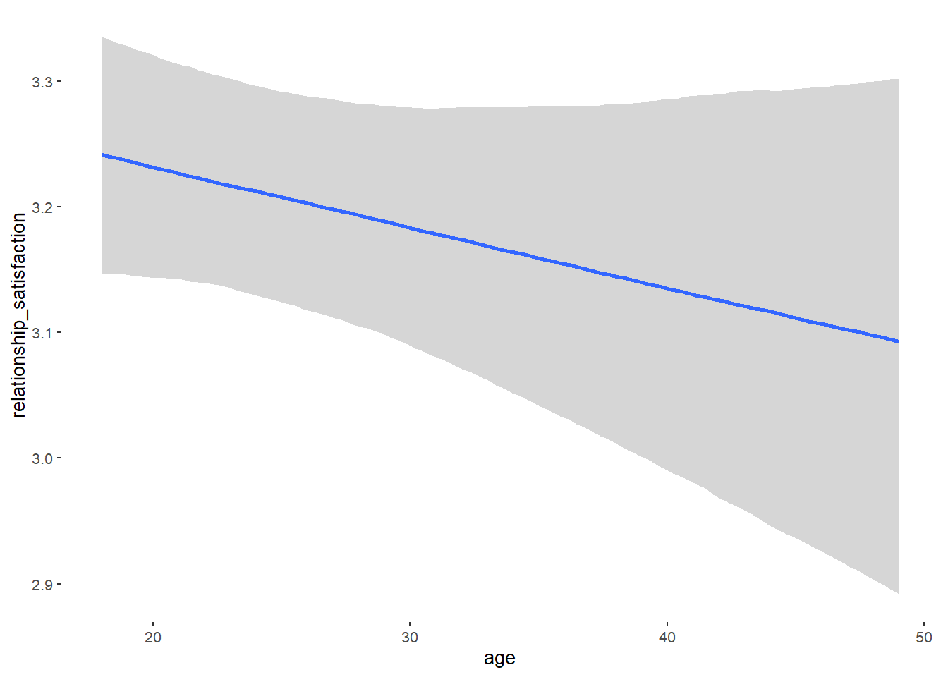
## age -0.00 0.00 -0.01 0.00 1.00 4011
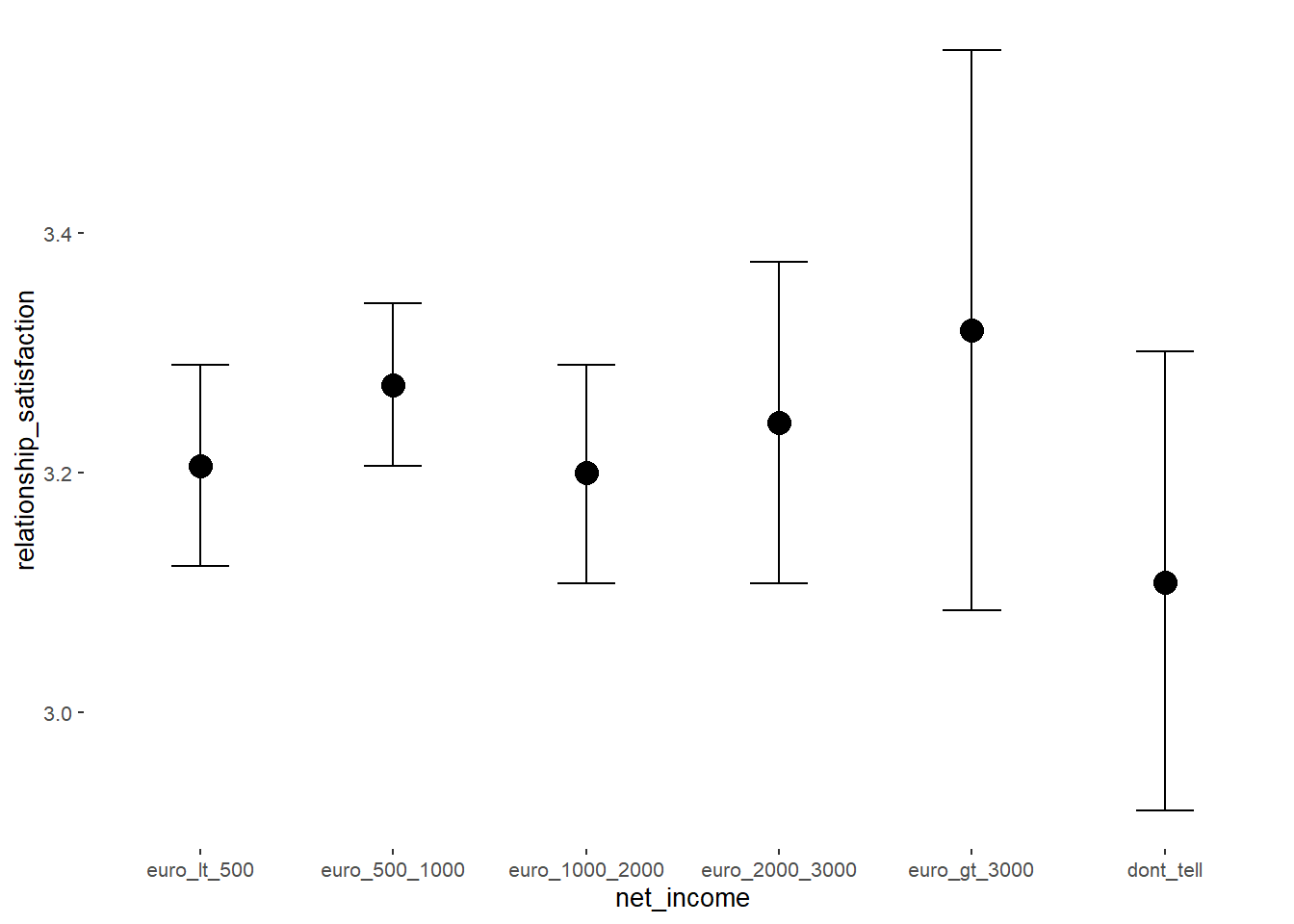
## net_incomeeuro_500_1000 0.07 0.04 0.01 0.13 1.00 3190
## net_incomeeuro_1000_2000 -0.01 0.05 -0.09 0.08 1.00 2692
## net_incomeeuro_2000_3000 0.04 0.07 -0.08 0.15 1.00 3233
## net_incomeeuro_gt_3000 0.11 0.12 -0.08 0.31 1.00 3668
## net_incomedont_tell -0.10 0.10 -0.26 0.07 1.00 4044
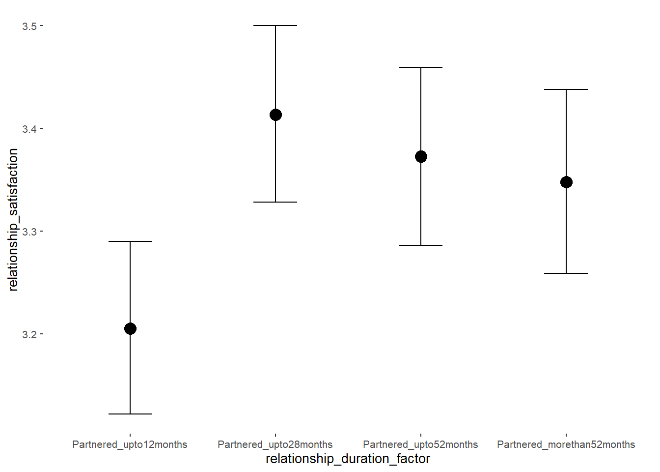
## relationship_duration_factorPartnered_upto28months 0.21 0.04 0.14 0.28 1.00 3251
## relationship_duration_factorPartnered_upto52months 0.17 0.04 0.10 0.24 1.00 3109
## relationship_duration_factorPartnered_morethan52months 0.14 0.04 0.07 0.21 1.00 3319
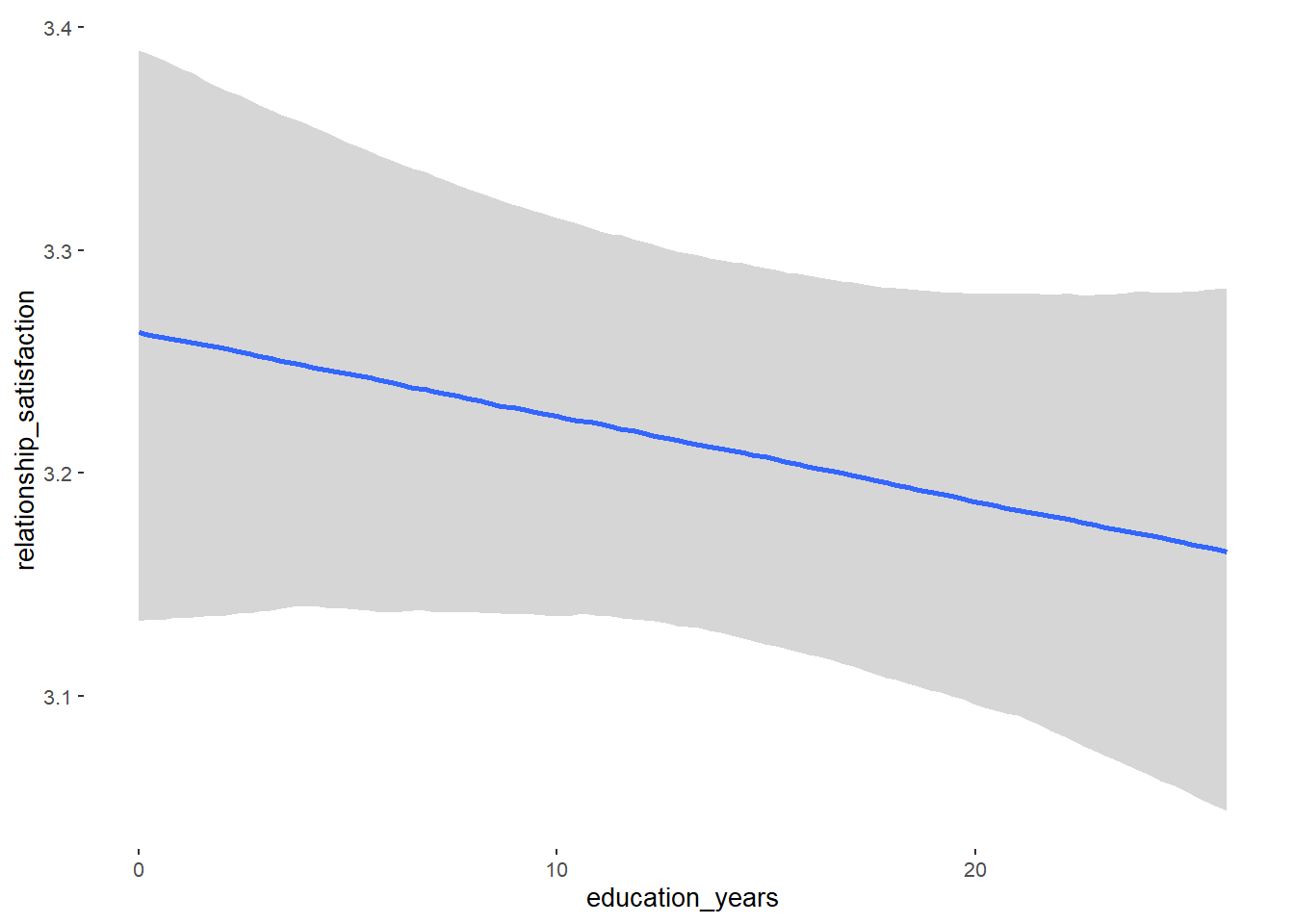
## education_years -0.00 0.00 -0.01 0.00 1.00 7198
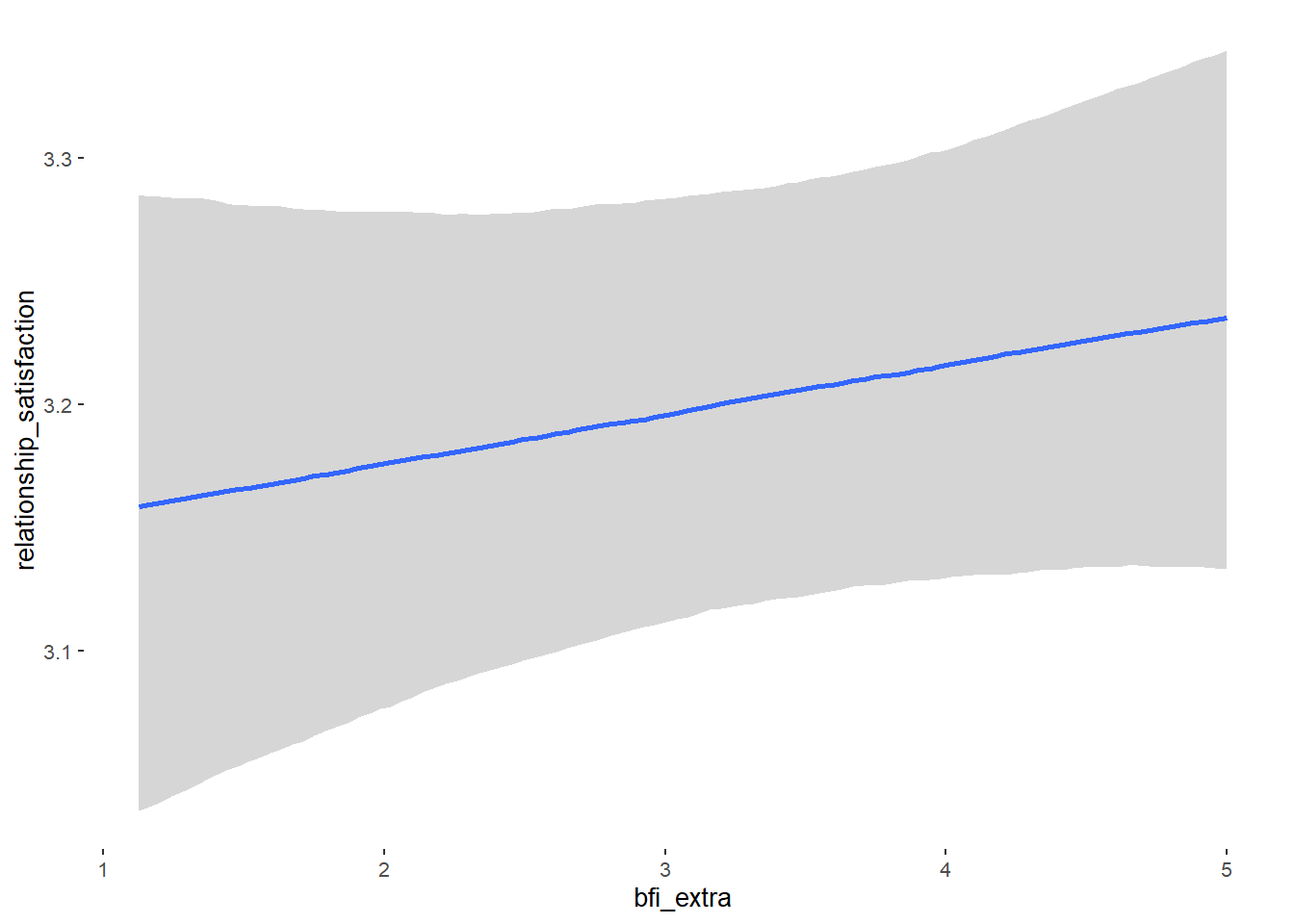
## bfi_extra 0.02 0.02 -0.01 0.05 1.00 4801
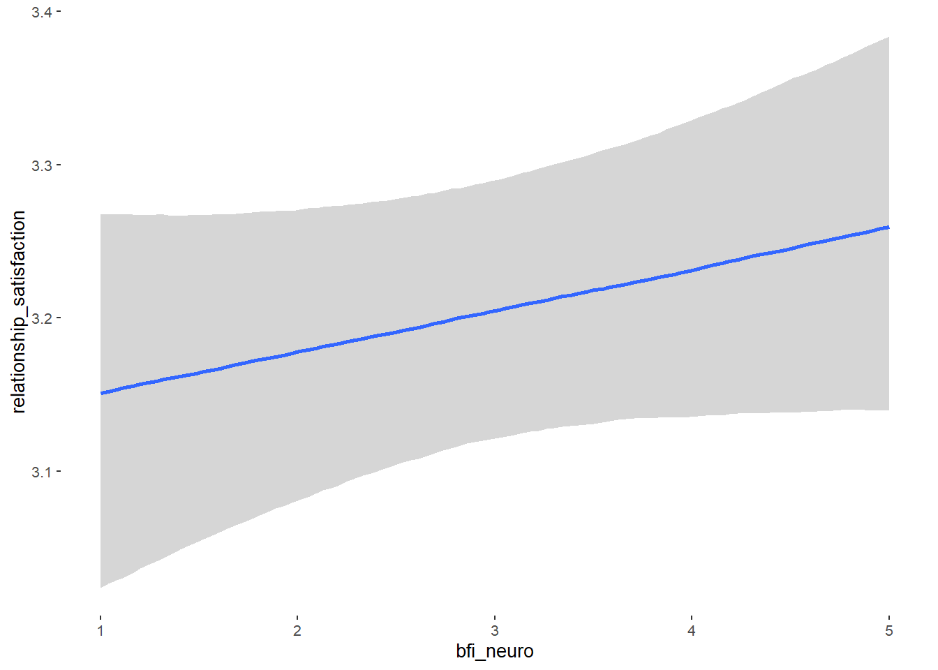
## bfi_neuro 0.03 0.02 -0.01 0.07 1.00 4013
## bfi_agree -0.02 0.03 -0.07 0.02 1.00 3944
## bfi_consc 0.00 0.02 -0.04 0.04 1.00 4361
## bfi_open -0.01 0.03 -0.06 0.03 1.00 4640
## religiosity 0.03 0.01 0.02 0.05 1.00 5147
## Tail_ESS
## Intercept 3130
## contraception_hormonalyes 3101
## age 3585
## net_incomeeuro_500_1000 3354
## net_incomeeuro_1000_2000 3107
## net_incomeeuro_2000_3000 3115
## net_incomeeuro_gt_3000 3275
## net_incomedont_tell 3320
## relationship_duration_factorPartnered_upto28months 3199
## relationship_duration_factorPartnered_upto52months 3115
## relationship_duration_factorPartnered_morethan52months 3246
## education_years 2915
## bfi_extra 3333
## bfi_neuro 2932
## bfi_agree 2854
## bfi_consc 2822
## bfi_open 3049
## religiosity 3279
##
## Family Specific Parameters:
## Estimate Est.Error l-90% CI u-90% CI Rhat Bulk_ESS Tail_ESS
## sigma 0.41 0.01 0.40 0.43 1.00 5262 3051
##
## Draws were sampled using sampling(NUTS). For each parameter, Bulk_ESS
## and Tail_ESS are effective sample size measures, and Rhat is the potential
## scale reduction factor on split chains (at convergence, Rhat = 1).Comparison with ROPE
plot(equivalence_test(m_hc_relsat_controlled, range = c(-0.04, 0.04), ci = 0.90,
                      parameters = "contraception"))
## Picking joint bandwidth of 0.00437## Warning: Removed 399 rows containing non-finite values (stat_density_ridges).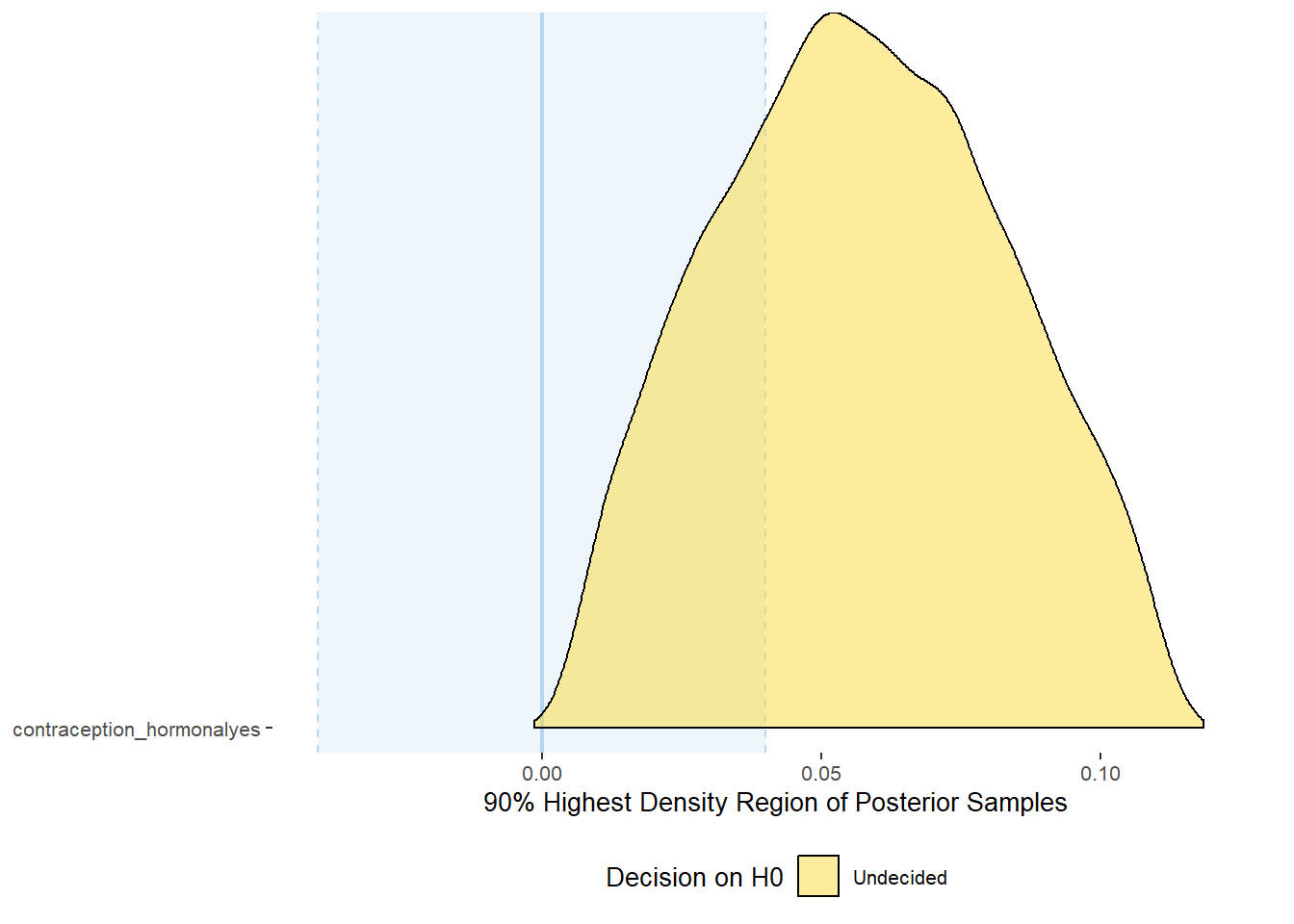
equivalence_test(m_hc_relsat_controlled, range = c(-0.04, 0.04), ci = 0.90,
                      parameters = "contraception")
## # A tibble: 1 x 10
## Parameter CI ROPE_low ROPE_high ROPE_Percentage ROPE_Equivalence HDI_low HDI_high Effects Component
## <chr> <dbl> <dbl> <dbl> <dbl> <chr> <dbl> <dbl> <chr> <chr>
## 1 b_contraceptio~ 0.9 -0.04 0.04 0.275 Undecided 0.00646 0.111 fixed conditio~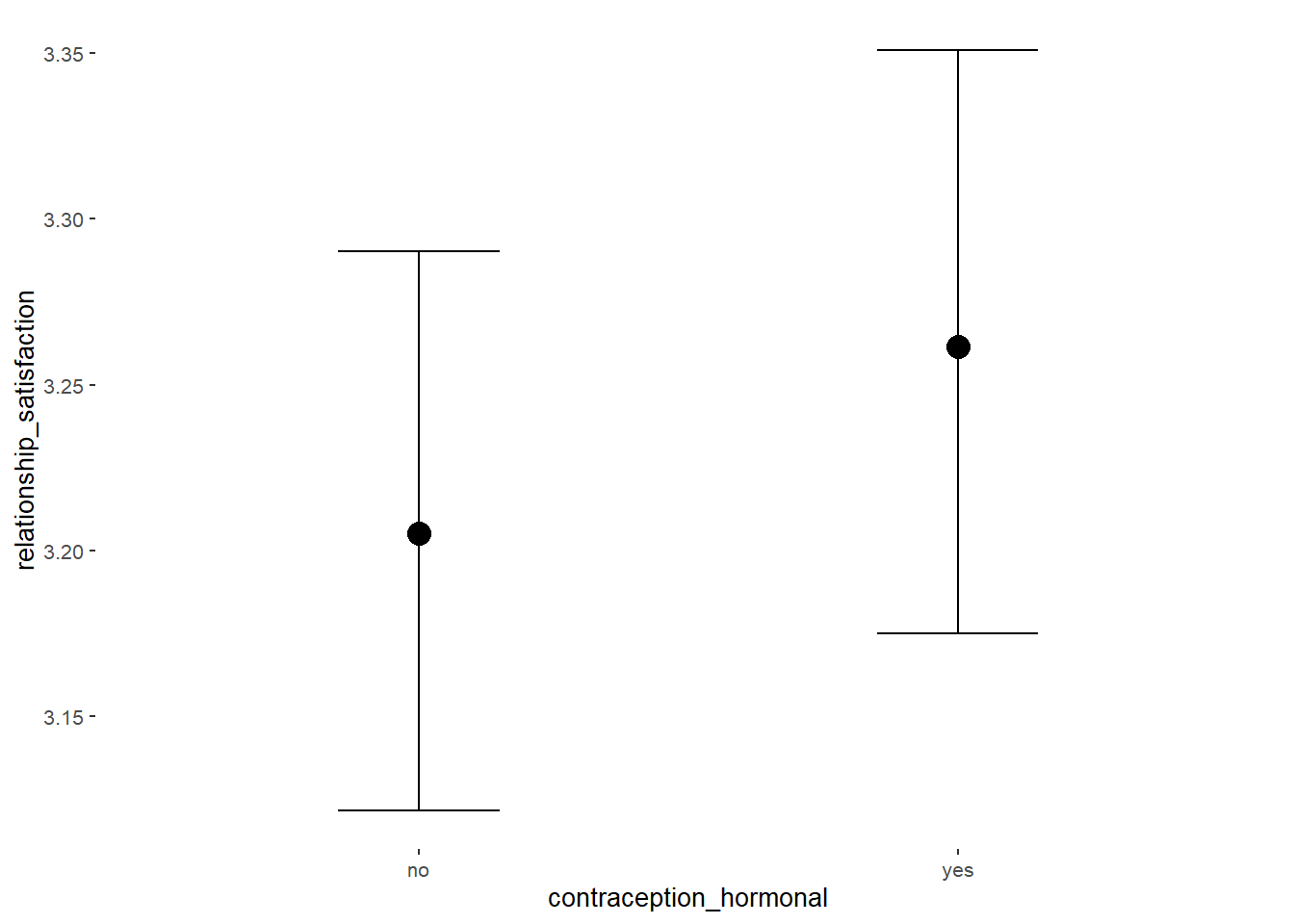
Forest Plot for Effect Sizes
m_hc_relsat_controlled %>%
  spread_draws(b_contraception_hormonalyes,
               b_age,
               b_net_incomeeuro_500_1000, b_net_incomeeuro_1000_2000,
               b_net_incomeeuro_2000_3000, b_net_incomeeuro_gt_3000, b_net_incomedont_tell,
               b_relationship_duration_factorPartnered_upto28months,
               b_relationship_duration_factorPartnered_upto52months,
               b_relationship_duration_factorPartnered_morethan52months,
               b_education_years,
               b_bfi_extra, b_bfi_neuro, b_bfi_agree, b_bfi_consc, b_bfi_open,
               b_religiosity) %>%
  pivot_longer(cols = c(b_contraception_hormonalyes,
                        b_age,
               b_net_incomeeuro_500_1000, b_net_incomeeuro_1000_2000,
               b_net_incomeeuro_2000_3000, b_net_incomeeuro_gt_3000, b_net_incomedont_tell,
               b_relationship_duration_factorPartnered_upto28months,
               b_relationship_duration_factorPartnered_upto52months,
               b_relationship_duration_factorPartnered_morethan52months,
               b_education_years,
               b_bfi_extra, b_bfi_neuro, b_bfi_agree, b_bfi_consc, b_bfi_open,
               b_religiosity),
               names_to = "condition",
               values_to = "r_condition") %>%
  mutate(condition_mean = r_condition,
         group = ifelse(condition %contains% "b_relationship_duration_factor",
                        "Relationship Duration",
                        ifelse(condition %contains% "b_net_income",
                               "Income",
                               NA)),
         group = ifelse(condition %contains% "b_contraception_hormonalyes",
                        "Contraception", group),
         condition = ifelse(condition %contains% "b_contraception_hormonalyes",
                        "Hormonal Contraception", condition),
         condition = ifelse(condition == "b_age", "Age",
                ifelse(condition == "b_net_incomeeuro_500_1000", "500-1000 Euro",
                ifelse(condition == "b_net_incomeeuro_1000_2000", "1000-2000 Euro",
                ifelse(condition == "b_net_incomeeuro_2000_3000", "2000-3000 Euro",
                ifelse(condition == "b_net_incomeeuro_gt_3000", ">3000 Euro",
                ifelse(condition == "b_net_incomedont_tell", "do not tell",
                ifelse(condition == "b_relationship_duration_factorPartnered_upto28months",
                       "13-28 months",
                ifelse(condition == "b_relationship_duration_factorPartnered_upto52months",
                       "29-52 months",
                ifelse(condition == "b_relationship_duration_factorPartnered_morethan52months",
                       ">52 months",
                ifelse(condition == "b_education_years", "Years of Education",
                ifelse(condition == "b_bfi_extra", "Extraversion",
                ifelse(condition == "b_bfi_neuro", "Neuroticism",
                ifelse(condition == "b_bfi_agree", "Agreeableness",
                ifelse(condition == "b_bfi_consc", "Conscientiousness",
                ifelse(condition == "b_bfi_open", "Openness",
                ifelse(condition == "b_religiosity", "Religiosity",
                       condition)))))))))))))))),
         group = ifelse(is.na(group), condition, group),
         condition = factor(condition, levels = rev(c("Hormonal Contraception", "Age",
                                        "500-1000 Euro", "1000-2000 Euro",
                                        "2000-3000 Euro", ">3000 Euro", "do not tell",
                                        "13-28 months", "29-52 months",
                                        ">52 months",
                                        "Years of Education",
                                        "Extraversion", "Neuroticism", "Agreeableness",
                                         "Conscientiousness","Openness","Religiosity"))),
         group = factor(group, levels = c("Contraception", "Age", "Income",
                                          "Relationship Duration","Years of Education",
                                          "Extraversion", "Neuroticism", "Agreeableness",
                                         "Conscientiousness","Openness","Religiosity"))) %>%
  ggplot(aes(y = condition,
             x = condition_mean,
             fill = stat(abs(x) < 0.04))) +
  stat_halfeye() +
  geom_vline(xintercept = c(-0.04, 0.04), linetype = "dotted") +
  apatheme +
  theme(legend.position = "none") +
  scale_fill_manual(values = c("gray80", "skyblue")) +
  labs(x = "Effect Size Estimates", y = "Predictors")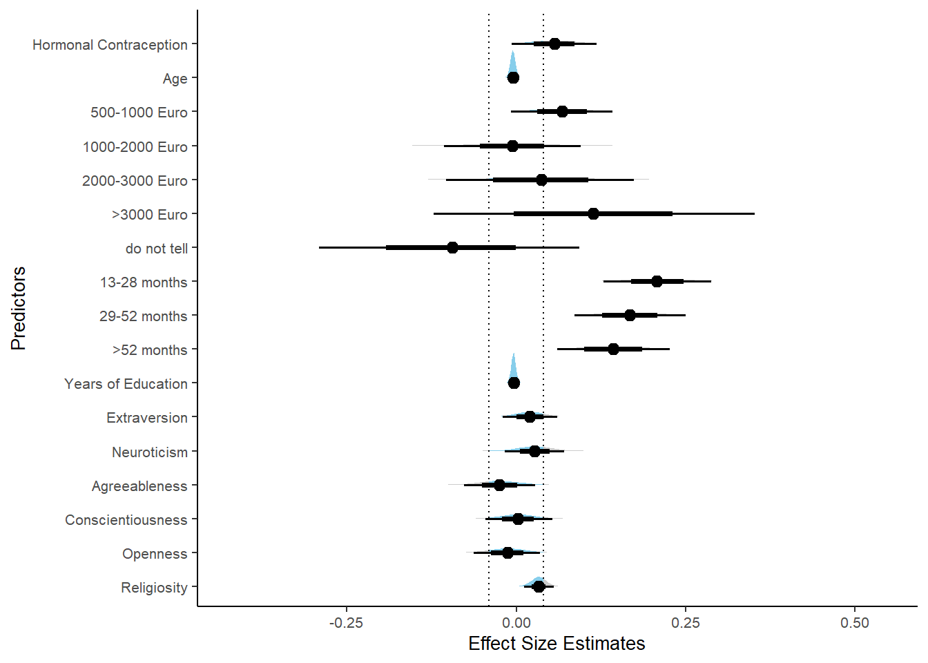
Sexual Satisfaction
Model
Summary
## Family: gaussian
## Links: mu = identity; sigma = identity
## Formula: satisfaction_sexual_intercourse ~ contraception_hormonal + age + net_income + relationship_duration_factor + education_years + bfi_extra + bfi_neuro + bfi_agree + bfi_consc + bfi_open + religiosity
## Data: data (Number of observations: 774)
## Draws: 4 chains, each with iter = 2000; warmup = 1000; thin = 1;
## total post-warmup draws = 4000
##
## Population-Level Effects:
## Estimate Est.Error l-90% CI u-90% CI Rhat Bulk_ESS
## Intercept 3.20 0.53 2.35 4.05 1.00 4370
## contraception_hormonalyes 0.11 0.08 -0.02 0.24 1.00 4602
## age 0.01 0.01 -0.01 0.02 1.00 3400
## net_incomeeuro_500_1000 0.03 0.10 -0.14 0.19 1.00 2752
## net_incomeeuro_1000_2000 -0.08 0.13 -0.29 0.13 1.00 2490
## net_incomeeuro_2000_3000 -0.08 0.17 -0.37 0.20 1.00 2779
## net_incomeeuro_gt_3000 -0.26 0.29 -0.73 0.22 1.00 4165
## net_incomedont_tell -0.04 0.25 -0.46 0.36 1.00 3354
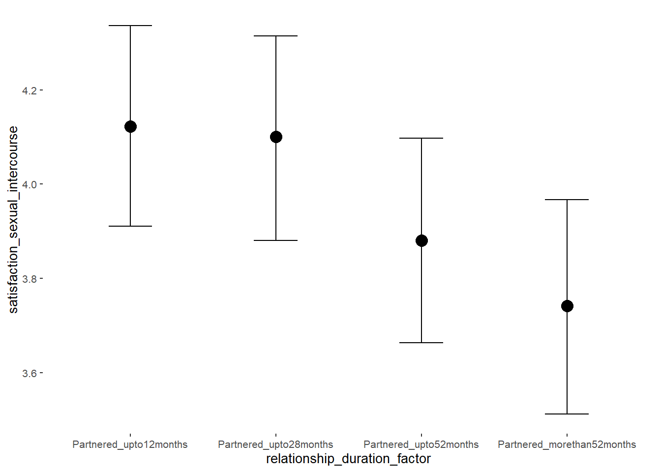
## relationship_duration_factorPartnered_upto28months -0.02 0.10 -0.19 0.15 1.00 3083
## relationship_duration_factorPartnered_upto52months -0.24 0.11 -0.42 -0.06 1.00 2824
## relationship_duration_factorPartnered_morethan52months -0.38 0.11 -0.57 -0.20 1.00 2557
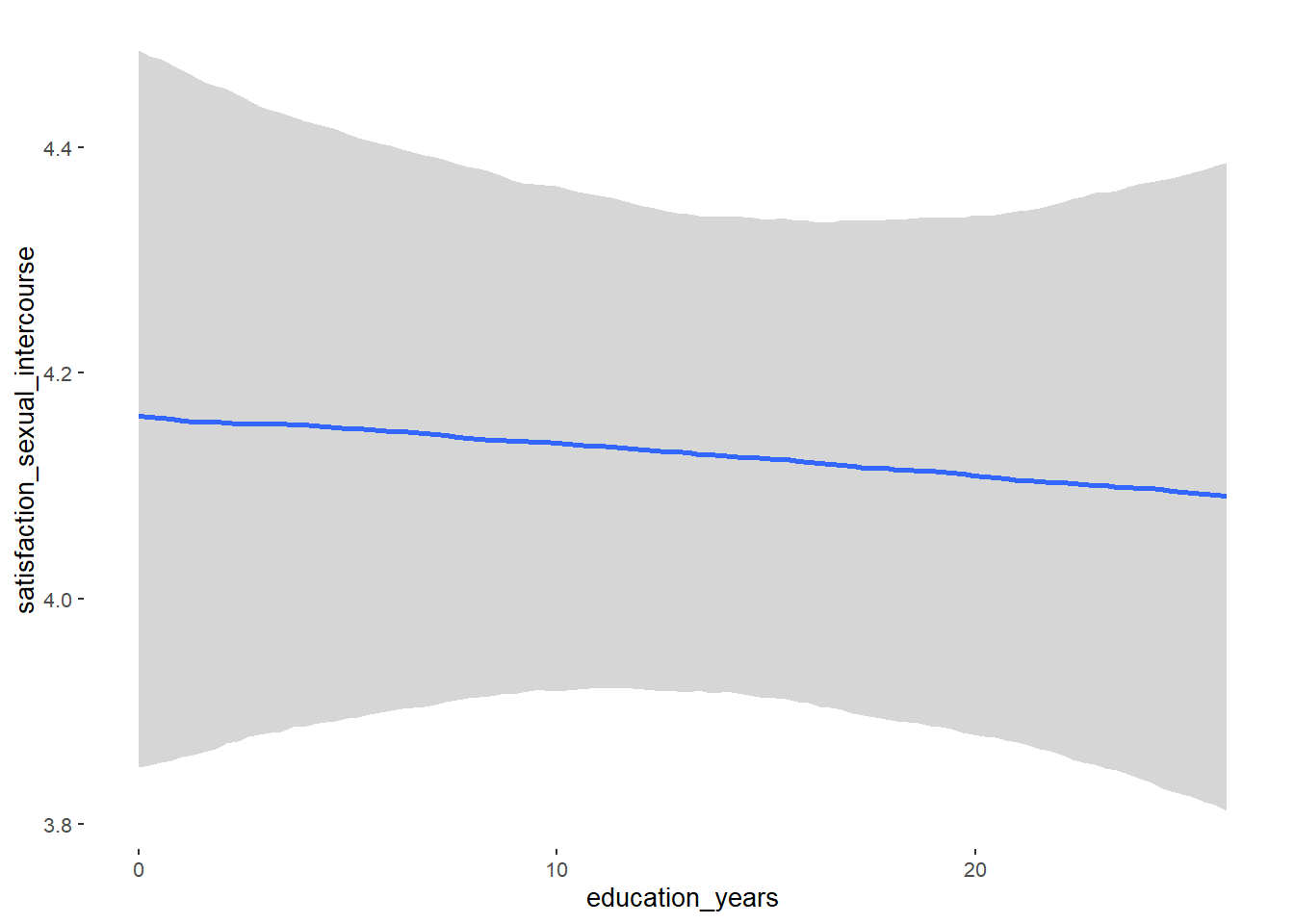
## education_years -0.00 0.01 -0.02 0.01 1.00 5674
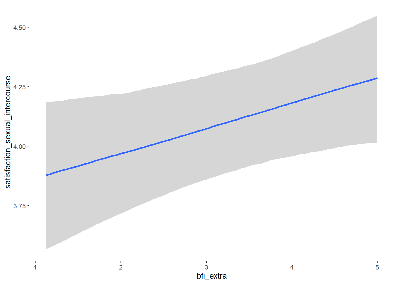
## bfi_extra 0.11 0.05 0.02 0.19 1.00 4252
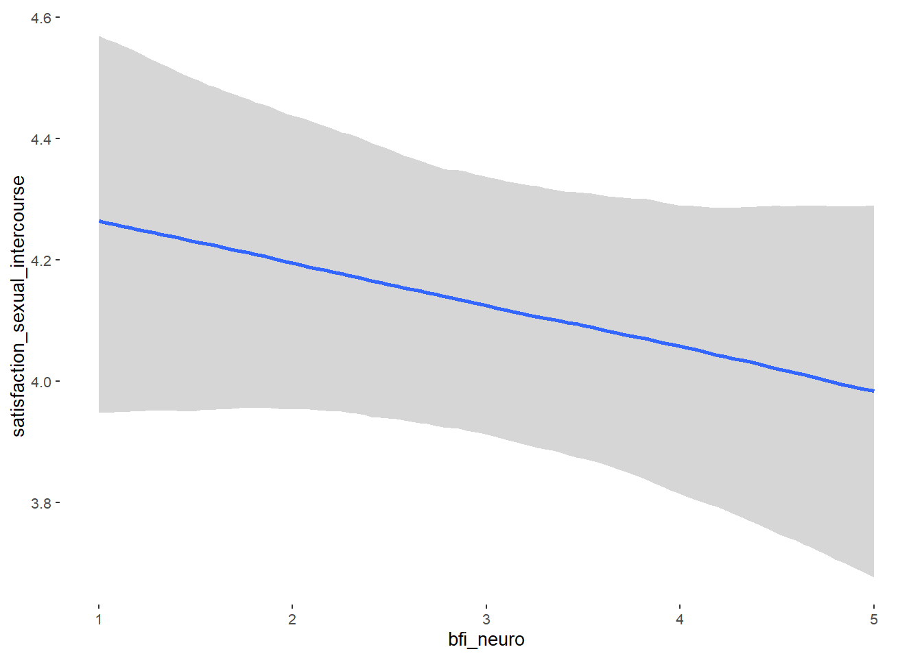
## bfi_neuro -0.07 0.06 -0.16 0.03 1.00 4347
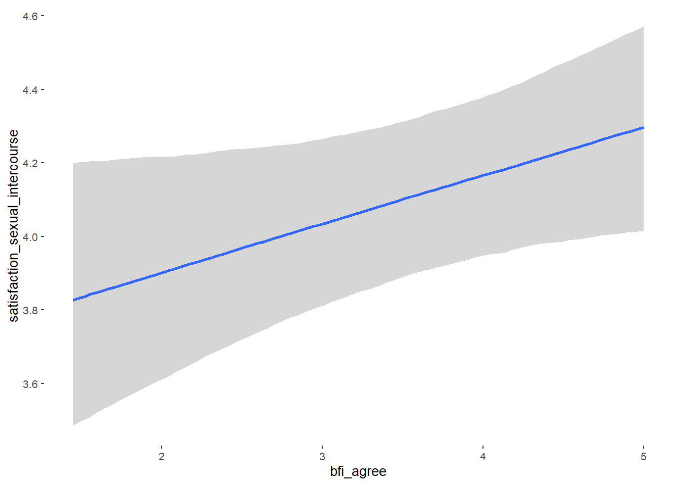
## bfi_agree 0.13 0.07 0.02 0.24 1.00 4543
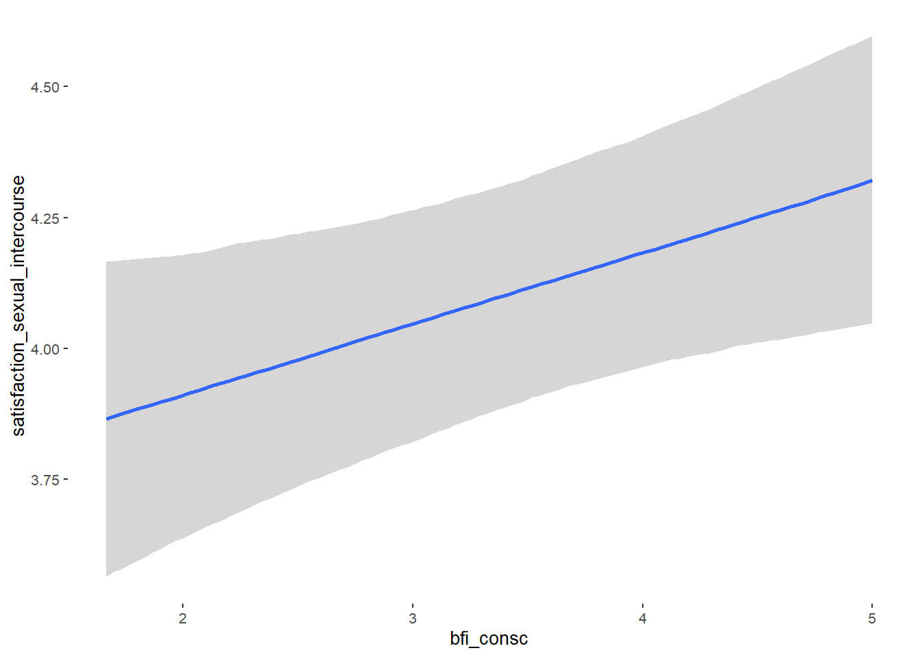
## bfi_consc 0.14 0.06 0.04 0.23 1.00 4518
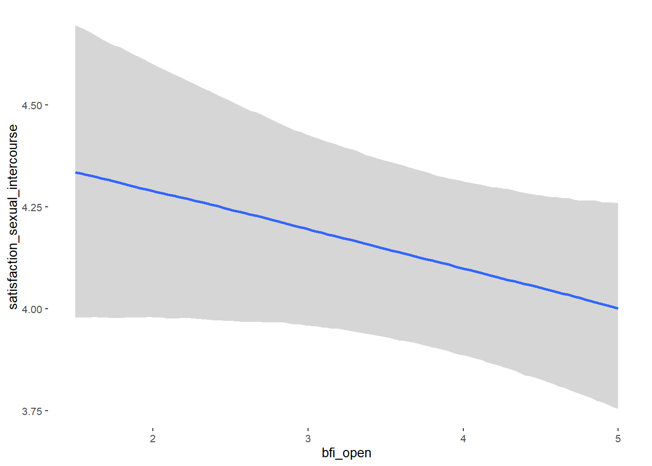
## bfi_open -0.10 0.06 -0.20 0.00 1.00 4654
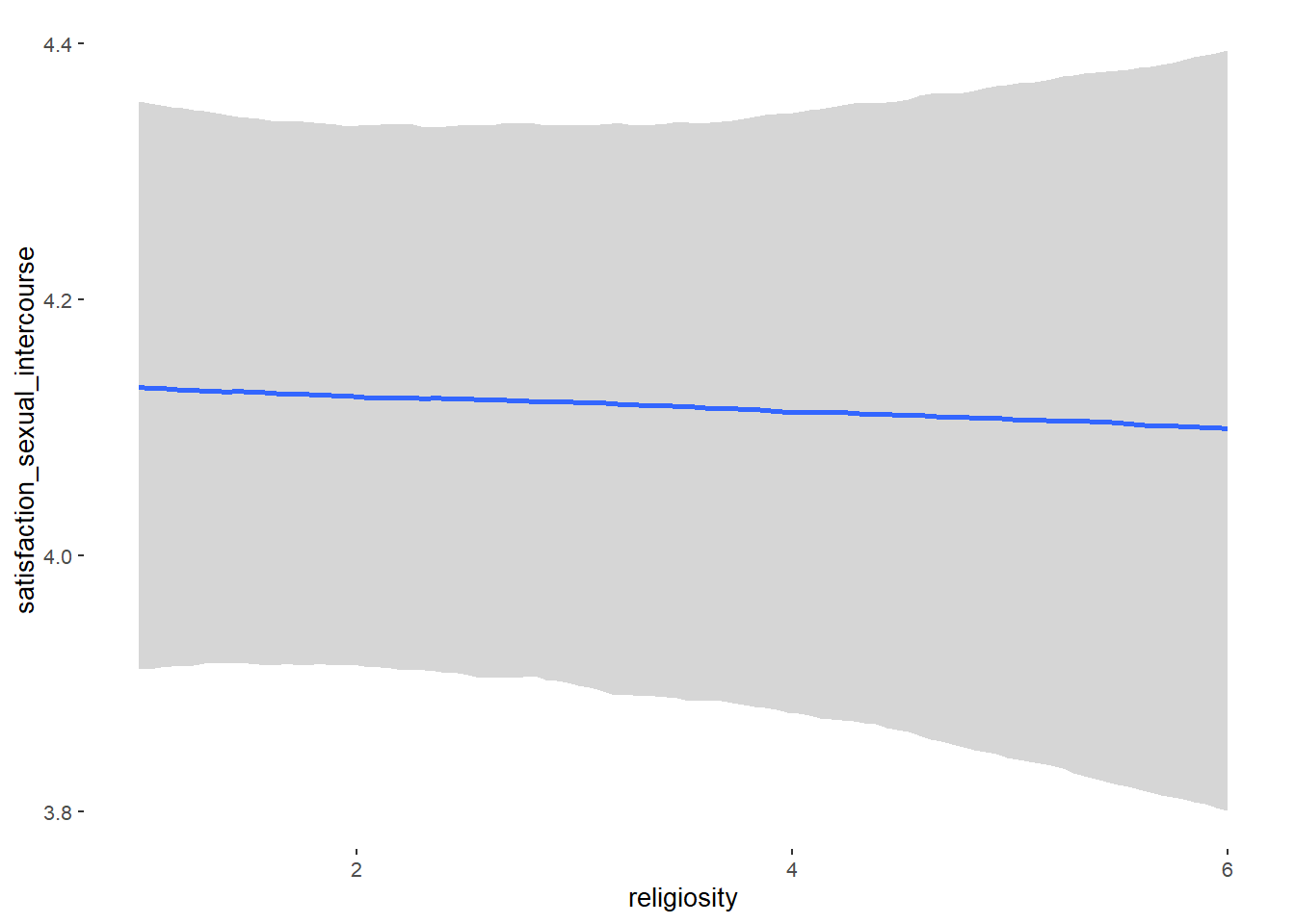
## religiosity -0.01 0.03 -0.05 0.04 1.00 5221
## Tail_ESS
## Intercept 3486
## contraception_hormonalyes 3157
## age 3264
## net_incomeeuro_500_1000 2829
## net_incomeeuro_1000_2000 2906
## net_incomeeuro_2000_3000 3014
## net_incomeeuro_gt_3000 3219
## net_incomedont_tell 3052
## relationship_duration_factorPartnered_upto28months 3211
## relationship_duration_factorPartnered_upto52months 3394
## relationship_duration_factorPartnered_morethan52months 2923
## education_years 2946
## bfi_extra 3350
## bfi_neuro 3131
## bfi_agree 3177
## bfi_consc 3165
## bfi_open 3259
## religiosity 3199
##
## Family Specific Parameters:
## Estimate Est.Error l-90% CI u-90% CI Rhat Bulk_ESS Tail_ESS
## sigma 1.03 0.03 0.99 1.07 1.00 5435 3222
##
## Draws were sampled using sampling(NUTS). For each parameter, Bulk_ESS
## and Tail_ESS are effective sample size measures, and Rhat is the potential
## scale reduction factor on split chains (at convergence, Rhat = 1).Comparison with ROPE
plot(equivalence_test(m_hc_sexsat_controlled, range = c(-0.11, 0.11), ci = 0.90,
                      parameters = "contraception"))
## Picking joint bandwidth of 0.0111## Warning: Removed 399 rows containing non-finite values (stat_density_ridges).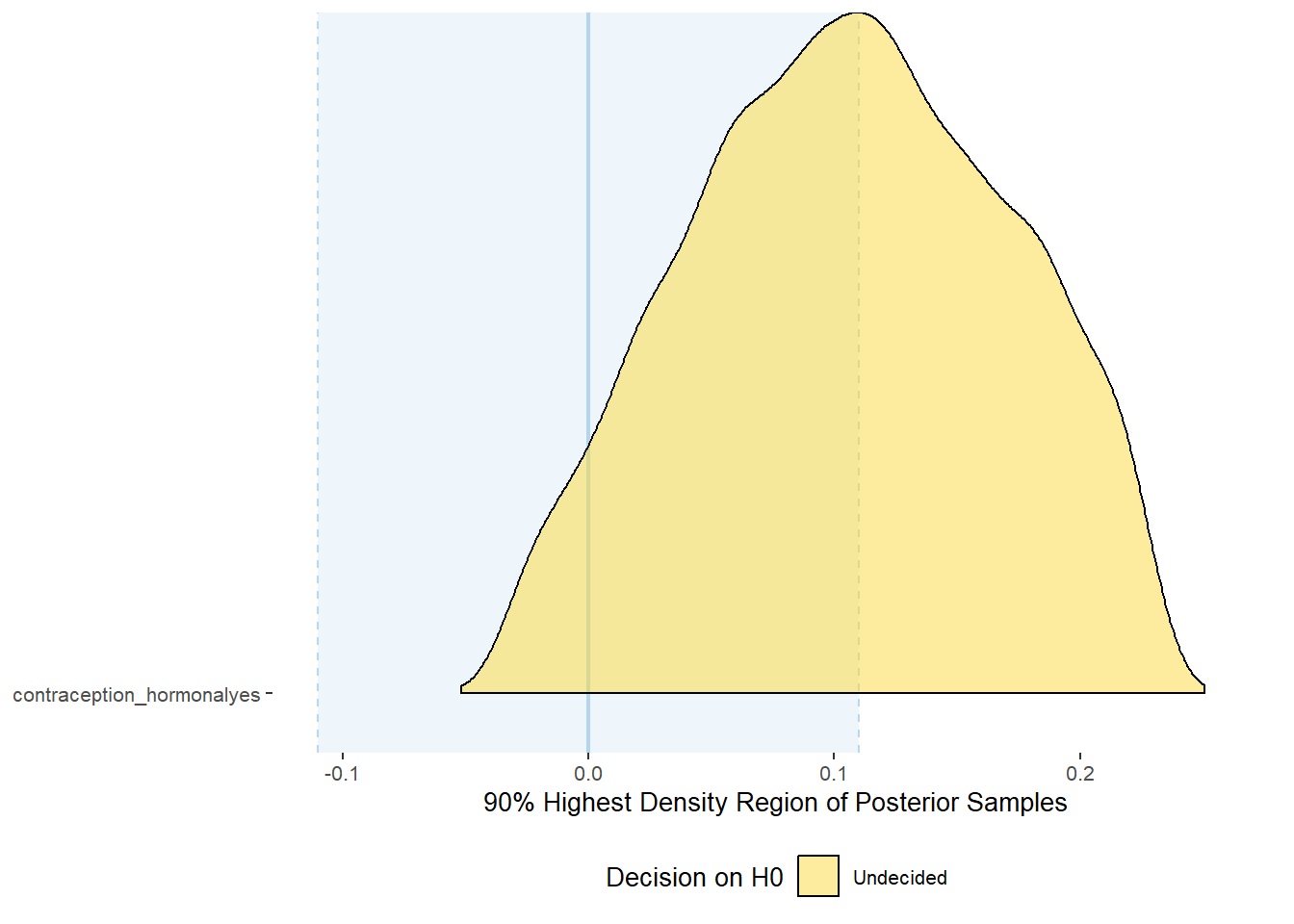
equivalence_test(m_hc_sexsat_controlled, range = c(-0.11, 0.11), ci = 0.90,
                      parameters = "contraception")
## # A tibble: 1 x 10
## Parameter CI ROPE_low ROPE_high ROPE_Percentage ROPE_Equivalence HDI_low HDI_high Effects Component
## <chr> <dbl> <dbl> <dbl> <dbl> <chr> <dbl> <dbl> <chr> <chr>
## 1 b_contraceptio~ 0.9 -0.11 0.11 0.518 Undecided -0.0319 0.230 fixed conditio~
Forest Plot for Effect Sizes
m_hc_sexsat_controlled %>%
  spread_draws(b_contraception_hormonalyes,
               b_age,
               b_net_incomeeuro_500_1000, b_net_incomeeuro_1000_2000,
               b_net_incomeeuro_2000_3000, b_net_incomeeuro_gt_3000, b_net_incomedont_tell,
               b_relationship_duration_factorPartnered_upto28months,
               b_relationship_duration_factorPartnered_upto52months,
               b_relationship_duration_factorPartnered_morethan52months,
               b_education_years,
               b_bfi_extra, b_bfi_neuro, b_bfi_agree, b_bfi_consc, b_bfi_open,
               b_religiosity) %>%
  pivot_longer(cols = c(b_contraception_hormonalyes,
                        b_age,
               b_net_incomeeuro_500_1000, b_net_incomeeuro_1000_2000,
               b_net_incomeeuro_2000_3000, b_net_incomeeuro_gt_3000, b_net_incomedont_tell,
               b_relationship_duration_factorPartnered_upto28months,
               b_relationship_duration_factorPartnered_upto52months,
               b_relationship_duration_factorPartnered_morethan52months,
               b_education_years,
               b_bfi_extra, b_bfi_neuro, b_bfi_agree, b_bfi_consc, b_bfi_open,
               b_religiosity),
               names_to = "condition",
               values_to = "r_condition") %>%
  mutate(condition_mean = r_condition,
         group = ifelse(condition %contains% "b_relationship_duration_factor",
                        "Relationship Duration",
                        ifelse(condition %contains% "b_net_income",
                               "Income",
                               NA)),
         group = ifelse(condition %contains% "b_contraception_hormonalyes",
                        "Contraception", group),
         condition = ifelse(condition %contains% "b_contraception_hormonalyes",
                        "Hormonal Contraception", condition),
         condition = ifelse(condition == "b_age", "Age",
                ifelse(condition == "b_net_incomeeuro_500_1000", "500-1000 Euro",
                ifelse(condition == "b_net_incomeeuro_1000_2000", "1000-2000 Euro",
                ifelse(condition == "b_net_incomeeuro_2000_3000", "2000-3000 Euro",
                ifelse(condition == "b_net_incomeeuro_gt_3000", ">3000 Euro",
                ifelse(condition == "b_net_incomedont_tell", "do not tell",
                ifelse(condition == "b_relationship_duration_factorPartnered_upto28months",
                       "13-28 months",
                ifelse(condition == "b_relationship_duration_factorPartnered_upto52months",
                       "29-52 months",
                ifelse(condition == "b_relationship_duration_factorPartnered_morethan52months",
                       ">52 months",
                ifelse(condition == "b_education_years", "Years of Education",
                ifelse(condition == "b_bfi_extra", "Extraversion",
                ifelse(condition == "b_bfi_neuro", "Neuroticism",
                ifelse(condition == "b_bfi_agree", "Agreeableness",
                ifelse(condition == "b_bfi_consc", "Conscientiousness",
                ifelse(condition == "b_bfi_open", "Openness",
                ifelse(condition == "b_religiosity", "Religiosity",
                       condition)))))))))))))))),
         group = ifelse(is.na(group), condition, group),
         condition = factor(condition, levels = rev(c("Hormonal Contraception", "Age",
                                        "500-1000 Euro", "1000-2000 Euro",
                                        "2000-3000 Euro", ">3000 Euro", "do not tell",
                                        "13-28 months", "29-52 months",
                                        ">52 months",
                                        "Years of Education",
                                        "Extraversion", "Neuroticism", "Agreeableness",
                                         "Conscientiousness","Openness","Religiosity"))),
         group = factor(group, levels = c("Contraception", "Age", "Income",
                                          "Relationship Duration","Years of Education",
                                          "Extraversion", "Neuroticism", "Agreeableness",
                                         "Conscientiousness","Openness","Religiosity"))) %>%
  ggplot(aes(y = condition,
             x = condition_mean,
             fill = stat(abs(x) < 0.11))) +
  stat_halfeye() +
  geom_vline(xintercept = c(-0.11, 0.11), linetype = "dotted") +
  apatheme +
  theme(legend.position = "none") +
  scale_fill_manual(values = c("gray80", "skyblue")) +
  labs(x = "Effect Size Estimates", y = "Predictors")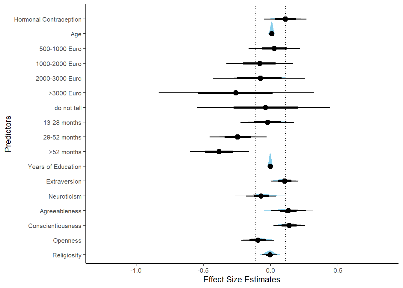
Libido
Model
Summary
## Family: gaussian
## Links: mu = identity; sigma = identity
## Formula: diary_libido_mean ~ contraception_hormonal + age + net_income + relationship_duration_factor + education_years + bfi_extra + bfi_neuro + bfi_agree + bfi_consc + bfi_open + religiosity
## Data: data (Number of observations: 968)
## Draws: 4 chains, each with iter = 2000; warmup = 1000; thin = 1;
## total post-warmup draws = 4000
##
## Population-Level Effects:
## Estimate Est.Error l-90% CI u-90% CI Rhat Bulk_ESS
## Intercept 0.27 0.26 -0.15 0.70 1.00 4585
## contraception_hormonalyes 0.00 0.04 -0.06 0.07 1.00 4109
## age 0.00 0.00 -0.00 0.01 1.00 3543
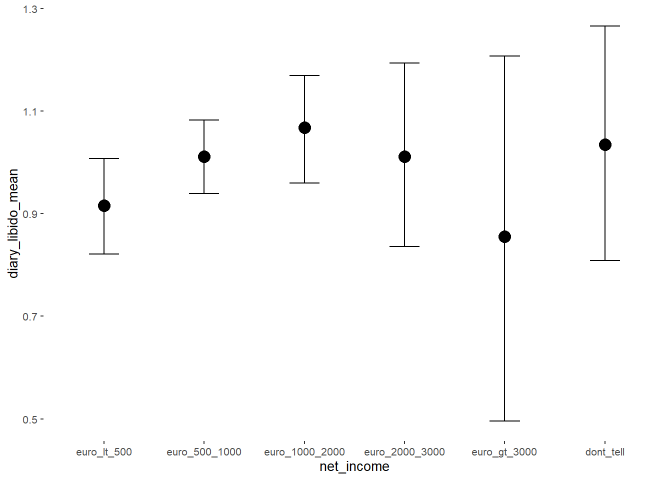
## net_incomeeuro_500_1000 0.10 0.05 0.02 0.17 1.00 2903
## net_incomeeuro_1000_2000 0.15 0.06 0.04 0.26 1.00 2443
## net_incomeeuro_2000_3000 0.10 0.10 -0.06 0.26 1.00 3429
## net_incomeeuro_gt_3000 -0.06 0.18 -0.35 0.24 1.00 4216
## net_incomedont_tell 0.12 0.12 -0.08 0.33 1.00 3409
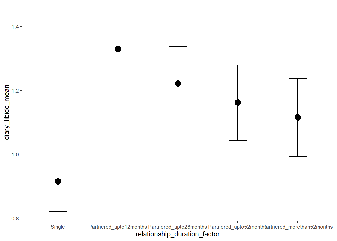
## relationship_duration_factorPartnered_upto12months 0.41 0.05 0.32 0.50 1.00 3379
## relationship_duration_factorPartnered_upto28months 0.31 0.05 0.22 0.39 1.00 3316
## relationship_duration_factorPartnered_upto52months 0.25 0.06 0.15 0.34 1.00 3128
## relationship_duration_factorPartnered_morethan52months 0.20 0.06 0.10 0.30 1.00 3302
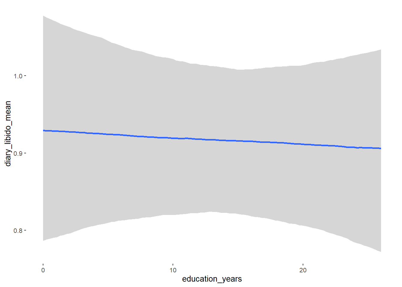
## education_years -0.00 0.00 -0.01 0.01 1.00 6409
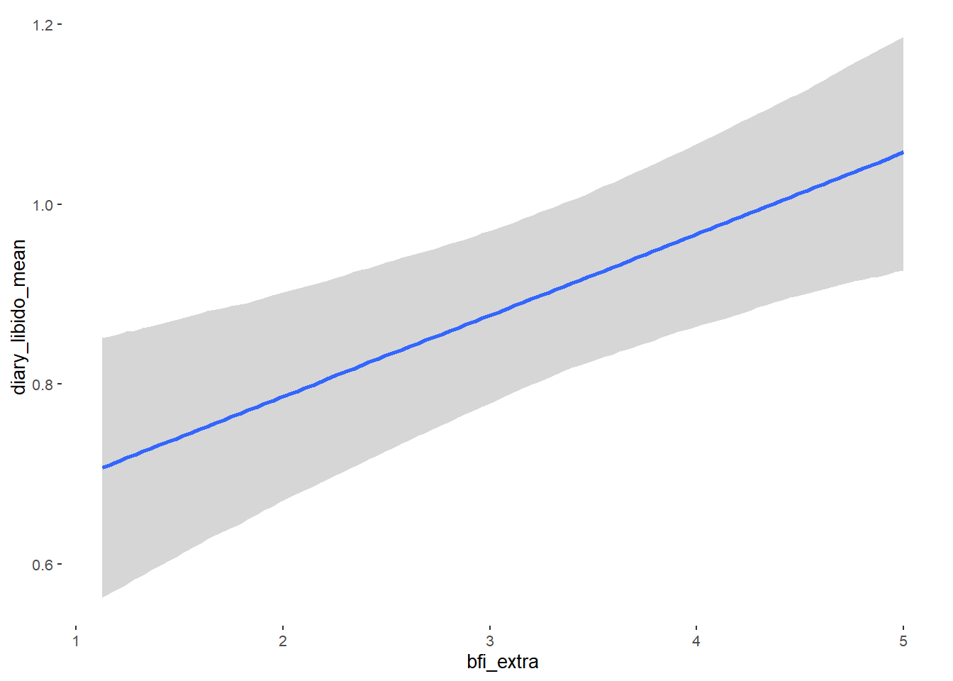
## bfi_extra 0.09 0.03 0.05 0.13 1.00 4187
## bfi_neuro -0.01 0.03 -0.06 0.03 1.00 4280
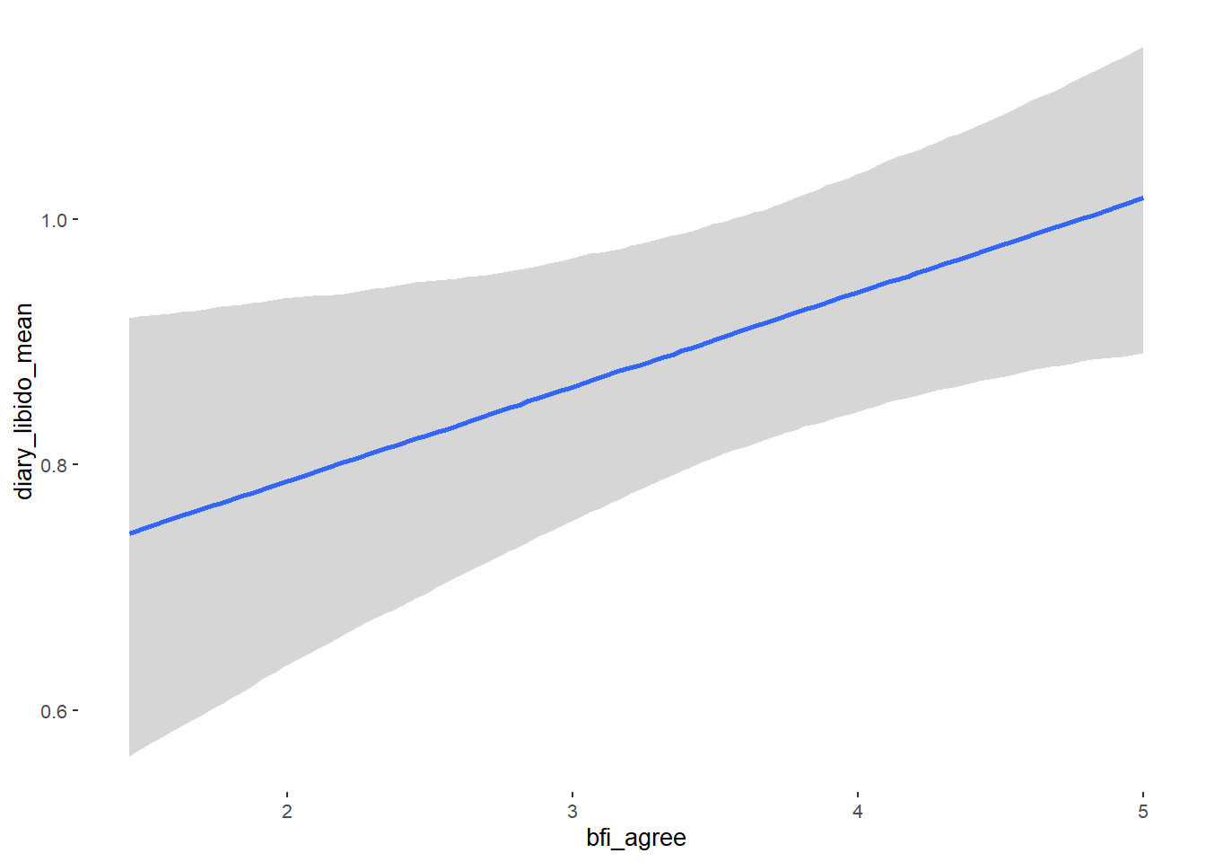
## bfi_agree 0.08 0.03 0.02 0.13 1.00 4350
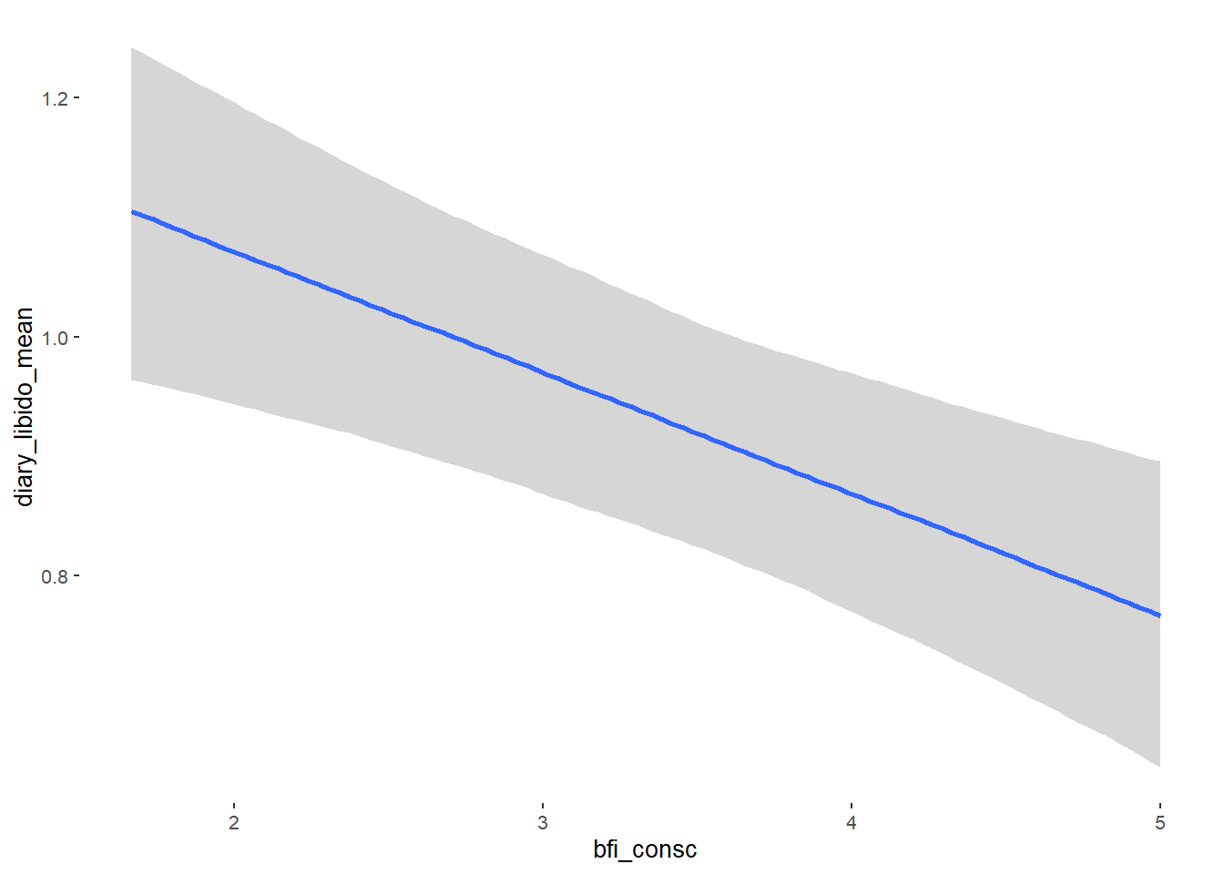
## bfi_consc -0.10 0.03 -0.15 -0.05 1.00 4833
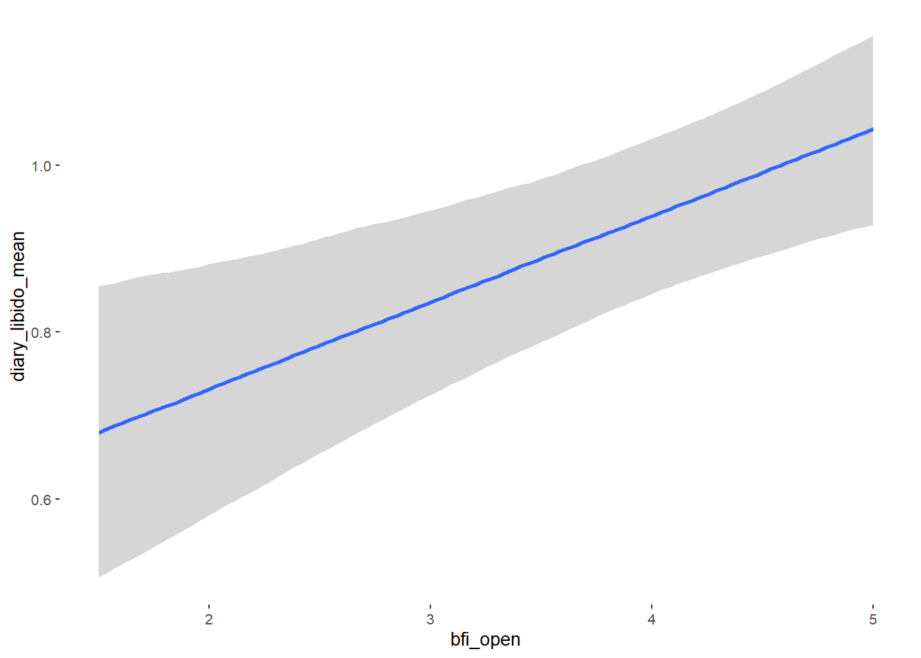
## bfi_open 0.10 0.03 0.05 0.15 1.00 3759
## religiosity -0.01 0.01 -0.03 0.02 1.00 5616
## Tail_ESS
## Intercept 3321
## contraception_hormonalyes 3244
## age 3209
## net_incomeeuro_500_1000 3187
## net_incomeeuro_1000_2000 3087
## net_incomeeuro_2000_3000 2672
## net_incomeeuro_gt_3000 2636
## net_incomedont_tell 3193
## relationship_duration_factorPartnered_upto12months 3115
## relationship_duration_factorPartnered_upto28months 3018
## relationship_duration_factorPartnered_upto52months 2549
## relationship_duration_factorPartnered_morethan52months 2786
## education_years 3125
## bfi_extra 3272
## bfi_neuro 3392
## bfi_agree 3264
## bfi_consc 3278
## bfi_open 2798
## religiosity 2937
##
## Family Specific Parameters:
## Estimate Est.Error l-90% CI u-90% CI Rhat Bulk_ESS Tail_ESS
## sigma 0.56 0.01 0.54 0.58 1.00 5416 3078
##
## Draws were sampled using sampling(NUTS). For each parameter, Bulk_ESS
## and Tail_ESS are effective sample size measures, and Rhat is the potential
## scale reduction factor on split chains (at convergence, Rhat = 1).Comparison with ROPE
plot(equivalence_test(m_hc_libido_controlled, range = c(-0.06, 0.06), ci = 0.90,
                      parameters = "contraception"))
## Picking joint bandwidth of 0.00559## Warning: Removed 399 rows containing non-finite values (stat_density_ridges).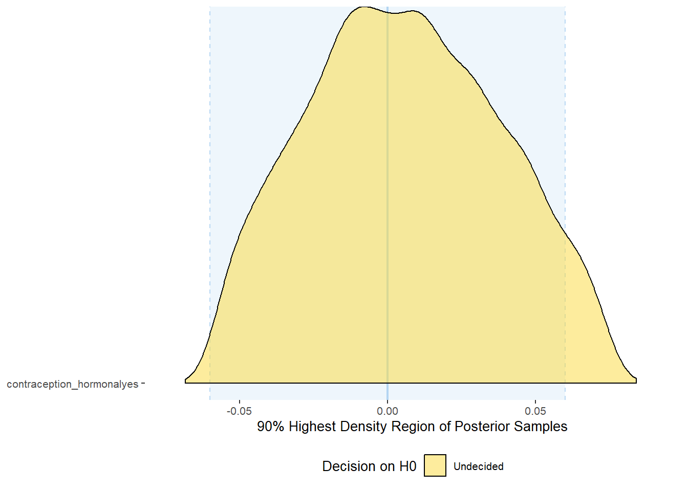
equivalence_test(m_hc_libido_controlled, range = c(-0.06, 0.06), ci = 0.90,
                      parameters = "contraception")
## # A tibble: 1 x 10
## Parameter CI ROPE_low ROPE_high ROPE_Percentage ROPE_Equivalence HDI_low HDI_high Effects Component
## <chr> <dbl> <dbl> <dbl> <dbl> <chr> <dbl> <dbl> <chr> <chr>
## 1 b_contraceptio~ 0.9 -0.06 0.06 0.949 Undecided -0.0570 0.0741 fixed conditio~
Forest Plot for Effect Sizes
m_hc_libido_controlled %>%
  spread_draws(b_contraception_hormonalyes,
               b_age,
               b_net_incomeeuro_500_1000, b_net_incomeeuro_1000_2000,
               b_net_incomeeuro_2000_3000, b_net_incomeeuro_gt_3000, b_net_incomedont_tell,
               b_relationship_duration_factorPartnered_upto28months,
               b_relationship_duration_factorPartnered_upto52months,
               b_relationship_duration_factorPartnered_morethan52months,
               b_education_years,
               b_bfi_extra, b_bfi_neuro, b_bfi_agree, b_bfi_consc, b_bfi_open,
               b_religiosity) %>%
  pivot_longer(cols = c(b_contraception_hormonalyes,
                        b_age,
               b_net_incomeeuro_500_1000, b_net_incomeeuro_1000_2000,
               b_net_incomeeuro_2000_3000, b_net_incomeeuro_gt_3000, b_net_incomedont_tell,
               b_relationship_duration_factorPartnered_upto28months,
               b_relationship_duration_factorPartnered_upto52months,
               b_relationship_duration_factorPartnered_morethan52months,
               b_education_years,
               b_bfi_extra, b_bfi_neuro, b_bfi_agree, b_bfi_consc, b_bfi_open,
               b_religiosity),
               names_to = "condition",
               values_to = "r_condition") %>%
  mutate(condition_mean = r_condition,
         group = ifelse(condition %contains% "b_relationship_duration_factor",
                        "Relationship Duration",
                        ifelse(condition %contains% "b_net_income",
                               "Income",
                               NA)),
         group = ifelse(condition %contains% "b_contraception_hormonalyes",
                        "Contraception", group),
         condition = ifelse(condition %contains% "b_contraception_hormonalyes",
                        "Hormonal Contraception", condition),
         condition = ifelse(condition == "b_age", "Age",
                ifelse(condition == "b_net_incomeeuro_500_1000", "500-1000 Euro",
                ifelse(condition == "b_net_incomeeuro_1000_2000", "1000-2000 Euro",
                ifelse(condition == "b_net_incomeeuro_2000_3000", "2000-3000 Euro",
                ifelse(condition == "b_net_incomeeuro_gt_3000", ">3000 Euro",
                ifelse(condition == "b_net_incomedont_tell", "do not tell",
                ifelse(condition == "b_relationship_duration_factorPartnered_upto28months",
                       "13-28 months",
                ifelse(condition == "b_relationship_duration_factorPartnered_upto52months",
                       "29-52 months",
                ifelse(condition == "b_relationship_duration_factorPartnered_morethan52months",
                       ">52 months",
                ifelse(condition == "b_education_years", "Years of Education",
                ifelse(condition == "b_bfi_extra", "Extraversion",
                ifelse(condition == "b_bfi_neuro", "Neuroticism",
                ifelse(condition == "b_bfi_agree", "Agreeableness",
                ifelse(condition == "b_bfi_consc", "Conscientiousness",
                ifelse(condition == "b_bfi_open", "Openness",
                ifelse(condition == "b_religiosity", "Religiosity",
                       condition)))))))))))))))),
         group = ifelse(is.na(group), condition, group),
         condition = factor(condition, levels = rev(c("Hormonal Contraception", "Age",
                                        "500-1000 Euro", "1000-2000 Euro",
                                        "2000-3000 Euro", ">3000 Euro", "do not tell",
                                        "13-28 months", "29-52 months",
                                        ">52 months",
                                        "Years of Education",
                                        "Extraversion", "Neuroticism", "Agreeableness",
                                         "Conscientiousness","Openness","Religiosity"))),
         group = factor(group, levels = c("Contraception", "Age", "Income",
                                          "Relationship Duration","Years of Education",
                                          "Extraversion", "Neuroticism", "Agreeableness",
                                         "Conscientiousness","Openness","Religiosity"))) %>%
  ggplot(aes(y = condition,
             x = condition_mean,
             fill = stat(abs(x) < 0.06))) +
  stat_halfeye() +
  geom_vline(xintercept = c(-0.06, 0.06), linetype = "dotted") +
  apatheme +
  theme(legend.position = "none") +
  scale_fill_manual(values = c("gray80", "skyblue")) +
  labs(x = "Effect Size Estimates", y = "Predictors")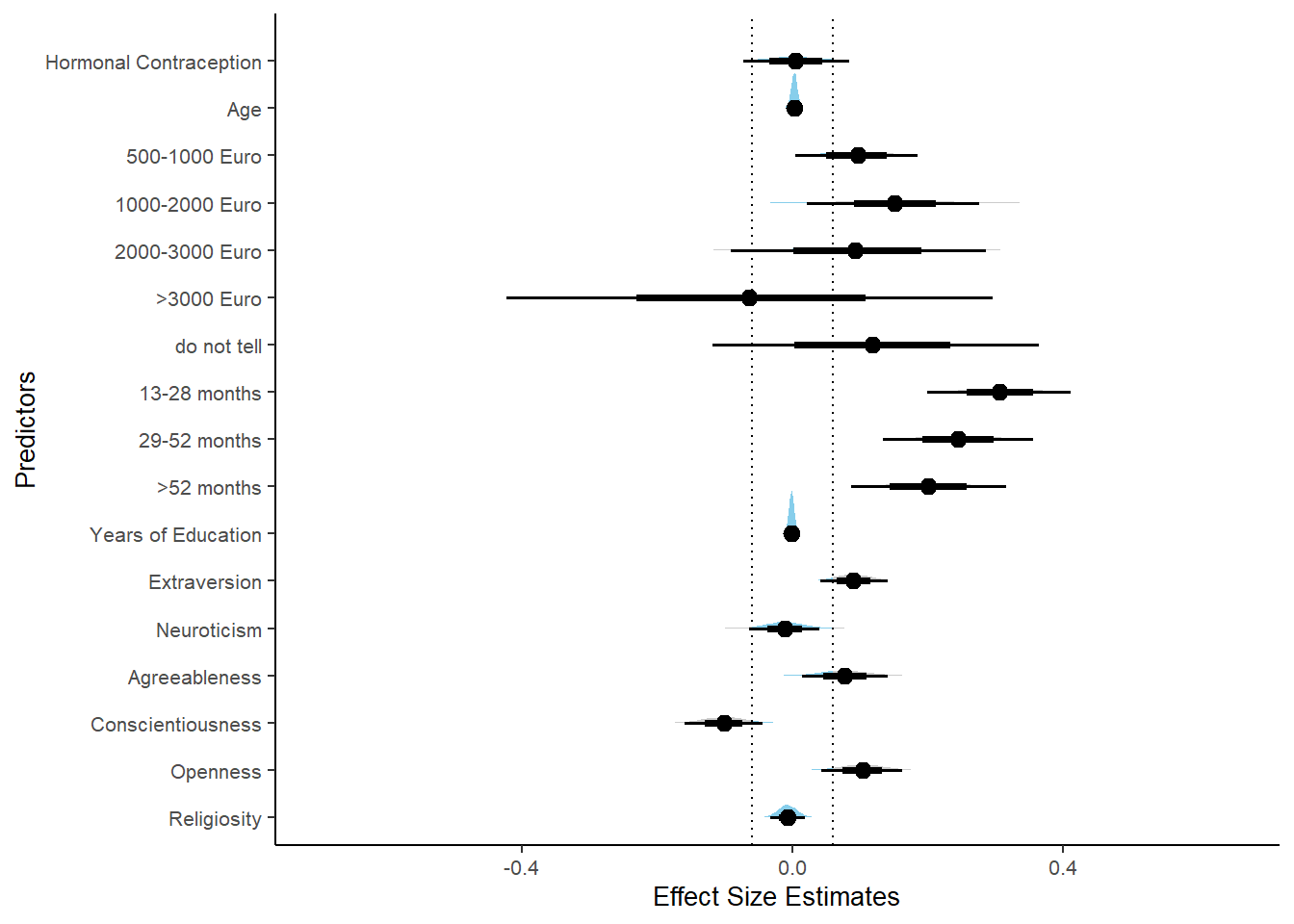
Sexual Frequency (Penetrative Intercourse)
Model
m_hc_sexfreqpen_controlled = brm(diary_sex_active_sex_sum ~
                        offset(log(number_of_days)) +
                        contraception_hormonal +
                        age + net_income + relationship_duration_factor +
                              education_years +
                              bfi_extra + bfi_neuro + bfi_agree + bfi_consc + bfi_open +
                              religiosity,
                data = data, family = poisson(),
                file = "m_hc_sexfreqpen_controlled")
Summary
##  Family: poisson
##   Links: mu = log
## Formula: diary_sex_active_sex_sum ~ offset(log(number_of_days)) + contraception_hormonal + age + net_income + relationship_duration_factor + education_years + bfi_extra + bfi_neuro + bfi_agree + bfi_consc + bfi_open + religiosity
##    Data: data (Number of observations: 897)
##   Draws: 4 chains, each with iter = 2000; warmup = 1000; thin = 1;
##          total post-warmup draws = 4000
##
## Population-Level Effects:
##                                                        Estimate Est.Error l-90% CI u-90% CI Rhat Bulk_ESS
## Intercept                                                 -3.35      0.18    -3.64    -3.06 1.00     4112
## contraception_hormonalyes                                  0.16      0.03     0.12     0.21 1.00     4523
## age                                                       -0.00      0.00    -0.01     0.01 1.00     3788
## net_incomeeuro_500_1000                                    0.16      0.03     0.11     0.21 1.00     2897
## net_incomeeuro_1000_2000                                   0.20      0.04     0.12     0.27 1.00     2694
## net_incomeeuro_2000_3000                                   0.38      0.06     0.28     0.47 1.00     2844
## net_incomeeuro_gt_3000                                     0.05      0.12    -0.14     0.24 1.00     3458
## net_incomedont_tell                                        0.45      0.07     0.32     0.56 1.00     3002
## relationship_duration_factorPartnered_upto12months         1.34      0.04     1.27     1.41 1.00     2312
## relationship_duration_factorPartnered_upto28months         1.22      0.04     1.15     1.29 1.00     2162
## relationship_duration_factorPartnered_upto52months         0.96      0.05     0.88     1.04 1.00     2430
## relationship_duration_factorPartnered_morethan52months     0.92      0.05     0.84     1.00 1.00     2440
## education_years                                           -0.01      0.00    -0.01    -0.01 1.00     6844
## bfi_extra                                                  0.01      0.02    -0.02     0.04 1.00     4316
## bfi_neuro                                                 -0.00      0.02    -0.03     0.03 1.00     3095
## bfi_agree                                                  0.09      0.02     0.06     0.13 1.00     4297
## bfi_consc                                                 -0.02      0.02    -0.05     0.02 1.00     3935
## bfi_open                                                   0.03      0.02    -0.00     0.06 1.00     3992
## religiosity                                               -0.01      0.01    -0.03     0.00 1.00     4416
##                                                        Tail_ESS
## Intercept                                                  3113
## contraception_hormonalyes                                  2707
## age                                                        3007
## net_incomeeuro_500_1000                                    3055
## net_incomeeuro_1000_2000                                   2973
## net_incomeeuro_2000_3000                                   2933
## net_incomeeuro_gt_3000                                     3126
## net_incomedont_tell                                        3336
## relationship_duration_factorPartnered_upto12months         2836
## relationship_duration_factorPartnered_upto28months         2620
## relationship_duration_factorPartnered_upto52months         2665
## relationship_duration_factorPartnered_morethan52months     2728
## education_years                                            3286
## bfi_extra                                                  2890
## bfi_neuro                                                  3132
## bfi_agree                                                  2658
## bfi_consc                                                  2976
## bfi_open                                                   3136
## religiosity                                                2969
##
## Draws were sampled using sampling(NUTS). For each parameter, Bulk_ESS
## and Tail_ESS are effective sample size measures, and Rhat is the potential
## scale reduction factor on split chains (at convergence, Rhat = 1).
Comparison with ROPE
plot(equivalence_test(m_hc_sexfreqpen_controlled, range = c(-0.05, 0.05), ci = 0.90,
                      parameters = "contraception"))
## Picking joint bandwidth of 0.00371## Warning: Removed 399 rows containing non-finite values (stat_density_ridges).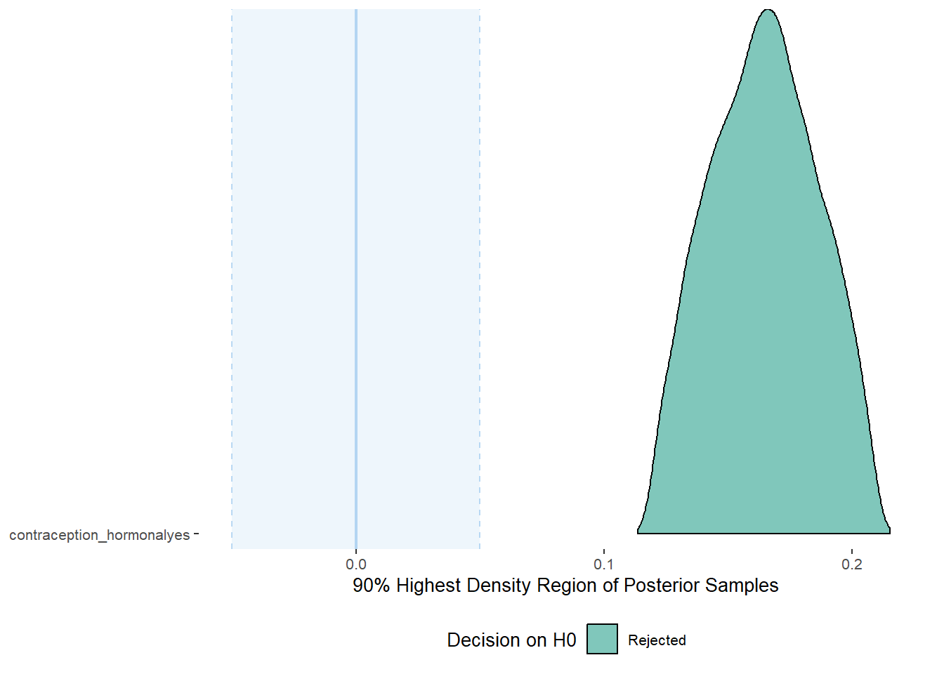
equivalence_test(m_hc_sexfreqpen_controlled, range = c(-0.05, 0.05), ci = 0.90,
                      parameters = "contraception")
## # A tibble: 1 x 10
## Parameter CI ROPE_low ROPE_high ROPE_Percentage ROPE_Equivalence HDI_low HDI_high Effects Component
## <chr> <dbl> <dbl> <dbl> <dbl> <chr> <dbl> <dbl> <chr> <chr>
## 1 b_contraceptio~ 0.9 -0.05 0.05 0 Rejected 0.120 0.209 fixed conditio~Plots
conditional_effects(m_hc_sexfreqpen_controlled,
                    effects = "contraception_hormonal",
                    conditions = data.frame(number_of_days = 1))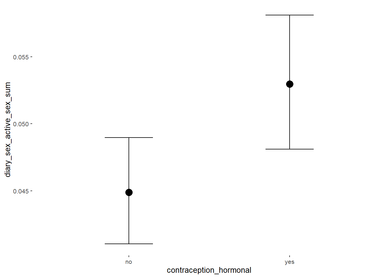
Forest Plot for Effect Sizes
m_hc_sexfreqpen_controlled %>%
  spread_draws(b_contraception_hormonalyes,
               b_age,
               b_net_incomeeuro_500_1000, b_net_incomeeuro_1000_2000,
               b_net_incomeeuro_2000_3000, b_net_incomeeuro_gt_3000, b_net_incomedont_tell,
               b_relationship_duration_factorPartnered_upto28months,
               b_relationship_duration_factorPartnered_upto52months,
               b_relationship_duration_factorPartnered_morethan52months,
               b_education_years,
               b_bfi_extra, b_bfi_neuro, b_bfi_agree, b_bfi_consc, b_bfi_open,
               b_religiosity) %>%
  pivot_longer(cols = c(b_contraception_hormonalyes,
                        b_age,
               b_net_incomeeuro_500_1000, b_net_incomeeuro_1000_2000,
               b_net_incomeeuro_2000_3000, b_net_incomeeuro_gt_3000, b_net_incomedont_tell,
               b_relationship_duration_factorPartnered_upto28months,
               b_relationship_duration_factorPartnered_upto52months,
               b_relationship_duration_factorPartnered_morethan52months,
               b_education_years,
               b_bfi_extra, b_bfi_neuro, b_bfi_agree, b_bfi_consc, b_bfi_open,
               b_religiosity),
               names_to = "condition",
               values_to = "r_condition") %>%
  mutate(condition_mean = r_condition,
         group = ifelse(condition %contains% "b_relationship_duration_factor",
                        "Relationship Duration",
                        ifelse(condition %contains% "b_net_income",
                               "Income",
                               NA)),
         group = ifelse(condition %contains% "b_contraception_hormonalyes",
                        "Contraception", group),
         condition = ifelse(condition %contains% "b_contraception_hormonalyes",
                        "Hormonal Contraception", condition),
         condition = ifelse(condition == "b_age", "Age",
                ifelse(condition == "b_net_incomeeuro_500_1000", "500-1000 Euro",
                ifelse(condition == "b_net_incomeeuro_1000_2000", "1000-2000 Euro",
                ifelse(condition == "b_net_incomeeuro_2000_3000", "2000-3000 Euro",
                ifelse(condition == "b_net_incomeeuro_gt_3000", ">3000 Euro",
                ifelse(condition == "b_net_incomedont_tell", "do not tell",
                ifelse(condition == "b_relationship_duration_factorPartnered_upto28months",
                       "13-28 months",
                ifelse(condition == "b_relationship_duration_factorPartnered_upto52months",
                       "29-52 months",
                ifelse(condition == "b_relationship_duration_factorPartnered_morethan52months",
                       ">52 months",
                ifelse(condition == "b_education_years", "Years of Education",
                ifelse(condition == "b_bfi_extra", "Extraversion",
                ifelse(condition == "b_bfi_neuro", "Neuroticism",
                ifelse(condition == "b_bfi_agree", "Agreeableness",
                ifelse(condition == "b_bfi_consc", "Conscientiousness",
                ifelse(condition == "b_bfi_open", "Openness",
                ifelse(condition == "b_religiosity", "Religiosity",
                       condition)))))))))))))))),
         group = ifelse(is.na(group), condition, group),
         condition = factor(condition, levels = rev(c("Hormonal Contraception", "Age",
                                        "500-1000 Euro", "1000-2000 Euro",
                                        "2000-3000 Euro", ">3000 Euro", "do not tell",
                                        "13-28 months", "29-52 months",
                                        ">52 months",
                                        "Years of Education",
                                        "Extraversion", "Neuroticism", "Agreeableness",
                                         "Conscientiousness","Openness","Religiosity"))),
         group = factor(group, levels = c("Contraception", "Age", "Income",
                                          "Relationship Duration","Years of Education",
                                          "Extraversion", "Neuroticism", "Agreeableness",
                                         "Conscientiousness","Openness","Religiosity"))) %>%
  ggplot(aes(y = condition,
             x = condition_mean,
             fill = stat(abs(x) < 0.05))) +
  stat_halfeye() +
  geom_vline(xintercept = c(-0.05, 0.05), linetype = "dotted") +
  apatheme +
  theme(legend.position = "none") +
  scale_fill_manual(values = c("gray80", "skyblue")) +
  labs(x = "Effect Size Estimates", y = "Predictors")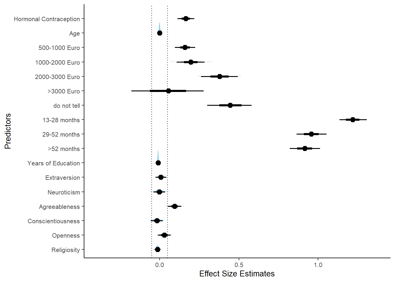
Masturabation Frequency
Model
m_hc_masfreq_controlled = brm(diary_masturbation_sum ~
                        offset(log(number_of_days)) +
                        contraception_hormonal +
                        age + net_income + relationship_duration_factor +
                              education_years +
                              bfi_extra + bfi_neuro + bfi_agree + bfi_consc + bfi_open +
                              religiosity,
                data = data, family = poisson(),
                file = "m_hc_masfreq_controlled")
Summary
##  Family: poisson
##   Links: mu = log
## Formula: diary_masturbation_sum ~ offset(log(number_of_days)) + contraception_hormonal + age + net_income + relationship_duration_factor + education_years + bfi_extra + bfi_neuro + bfi_agree + bfi_consc + bfi_open + religiosity
##    Data: data (Number of observations: 897)
##   Draws: 4 chains, each with iter = 2000; warmup = 1000; thin = 1;
##          total post-warmup draws = 4000
##
## Population-Level Effects:
##                                                        Estimate Est.Error l-90% CI u-90% CI Rhat Bulk_ESS
## Intercept                                                 -1.67      0.19    -1.97    -1.36 1.00     3446
## contraception_hormonalyes                                 -0.30      0.03    -0.34    -0.25 1.00     4457
## age                                                       -0.00      0.00    -0.01     0.00 1.00     4539
## net_incomeeuro_500_1000                                    0.18      0.03     0.13     0.24 1.00     3225
## net_incomeeuro_1000_2000                                   0.21      0.05     0.14     0.29 1.00     3055
## net_incomeeuro_2000_3000                                   0.05      0.07    -0.07     0.16 1.00     3731
## net_incomeeuro_gt_3000                                    -0.18      0.14    -0.42     0.05 1.00     4737
## net_incomedont_tell                                       -0.22      0.10    -0.39    -0.05 1.00     4168
## relationship_duration_factorPartnered_upto12months        -0.20      0.04    -0.26    -0.14 1.00     3456
## relationship_duration_factorPartnered_upto28months        -0.23      0.04    -0.30    -0.17 1.00     3757
## relationship_duration_factorPartnered_upto52months        -0.30      0.04    -0.36    -0.23 1.00     2965
## relationship_duration_factorPartnered_morethan52months    -0.44      0.04    -0.51    -0.36 1.00     3239
## education_years                                            0.00      0.00    -0.00     0.01 1.00     6532
## bfi_extra                                                 -0.01      0.02    -0.04     0.02 1.00     3812
## bfi_neuro                                                 -0.01      0.02    -0.04     0.02 1.00     3190
## bfi_agree                                                  0.00      0.02    -0.03     0.04 1.00     3875
## bfi_consc                                                 -0.21      0.02    -0.24    -0.17 1.00     4267
## bfi_open                                                   0.20      0.02     0.17     0.24 1.00     4291
## religiosity                                               -0.06      0.01    -0.07    -0.04 1.00     4998
##                                                        Tail_ESS
## Intercept                                                  2984
## contraception_hormonalyes                                  3346
## age                                                        3623
## net_incomeeuro_500_1000                                    3116
## net_incomeeuro_1000_2000                                   3063
## net_incomeeuro_2000_3000                                   3058
## net_incomeeuro_gt_3000                                     3281
## net_incomedont_tell                                        2963
## relationship_duration_factorPartnered_upto12months         2802
## relationship_duration_factorPartnered_upto28months         3112
## relationship_duration_factorPartnered_upto52months         2478
## relationship_duration_factorPartnered_morethan52months     3304
## education_years                                            3193
## bfi_extra                                                  3226
## bfi_neuro                                                  2866
## bfi_agree                                                  2797
## bfi_consc                                                  3059
## bfi_open                                                   2873
## religiosity                                                3165
##
## Draws were sampled using sampling(NUTS). For each parameter, Bulk_ESS
## and Tail_ESS are effective sample size measures, and Rhat is the potential
## scale reduction factor on split chains (at convergence, Rhat = 1).
Comparison with ROPE
plot(equivalence_test(m_hc_masfreq_controlled, range = c(-0.05, 0.05), ci = 0.90,
                      parameters = "contraception"))
## Picking joint bandwidth of 0.00384## Warning: Removed 399 rows containing non-finite values (stat_density_ridges).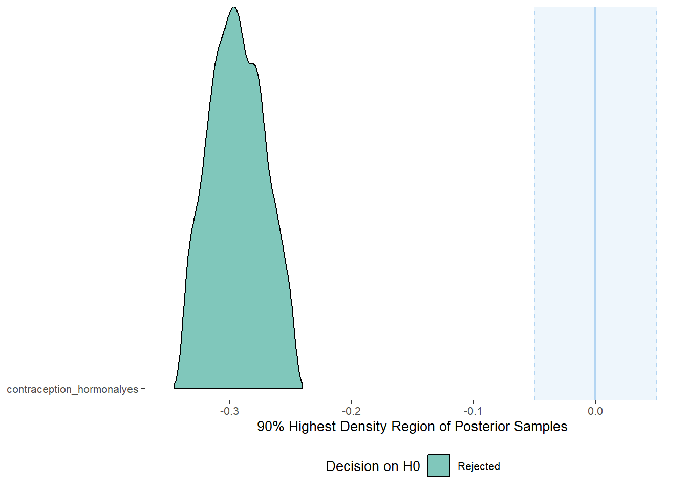
equivalence_test(m_hc_masfreq_controlled, range = c(-0.05, 0.05), ci = 0.90,
                      parameters = "contraception")
## # A tibble: 1 x 10
## Parameter CI ROPE_low ROPE_high ROPE_Percentage ROPE_Equivalence HDI_low HDI_high Effects Component
## <chr> <dbl> <dbl> <dbl> <dbl> <chr> <dbl> <dbl> <chr> <chr>
## 1 b_contraceptio~ 0.9 -0.05 0.05 0 Rejected -0.338 -0.248 fixed conditio~Plots
conditional_effects(m_hc_masfreq_controlled,
                    effects = "contraception_hormonal",
                    conditions = data.frame(number_of_days = 1))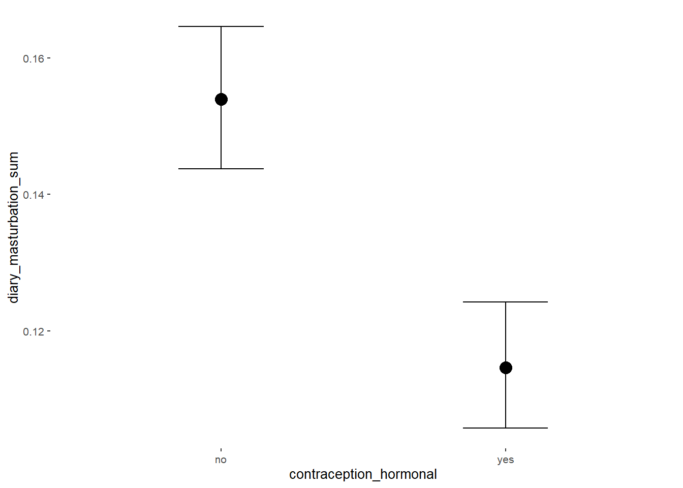
Forest Plot for Effect Sizes
m_hc_masfreq_controlled %>%
  spread_draws(b_contraception_hormonalyes,
               b_age,
               b_net_incomeeuro_500_1000, b_net_incomeeuro_1000_2000,
               b_net_incomeeuro_2000_3000, b_net_incomeeuro_gt_3000, b_net_incomedont_tell,
               b_relationship_duration_factorPartnered_upto28months,
               b_relationship_duration_factorPartnered_upto52months,
               b_relationship_duration_factorPartnered_morethan52months,
               b_education_years,
               b_bfi_extra, b_bfi_neuro, b_bfi_agree, b_bfi_consc, b_bfi_open,
               b_religiosity) %>%
  pivot_longer(cols = c(b_contraception_hormonalyes,
                        b_age,
               b_net_incomeeuro_500_1000, b_net_incomeeuro_1000_2000,
               b_net_incomeeuro_2000_3000, b_net_incomeeuro_gt_3000, b_net_incomedont_tell,
               b_relationship_duration_factorPartnered_upto28months,
               b_relationship_duration_factorPartnered_upto52months,
               b_relationship_duration_factorPartnered_morethan52months,
               b_education_years,
               b_bfi_extra, b_bfi_neuro, b_bfi_agree, b_bfi_consc, b_bfi_open,
               b_religiosity),
               names_to = "condition",
               values_to = "r_condition") %>%
  mutate(condition_mean = r_condition,
         group = ifelse(condition %contains% "b_relationship_duration_factor",
                        "Relationship Duration",
                        ifelse(condition %contains% "b_net_income",
                               "Income",
                               NA)),
         group = ifelse(condition %contains% "b_contraception_hormonalyes",
                        "Contraception", group),
         condition = ifelse(condition %contains% "b_contraception_hormonalyes",
                        "Hormonal Contraception", condition),
         condition = ifelse(condition == "b_age", "Age",
                ifelse(condition == "b_net_incomeeuro_500_1000", "500-1000 Euro",
                ifelse(condition == "b_net_incomeeuro_1000_2000", "1000-2000 Euro",
                ifelse(condition == "b_net_incomeeuro_2000_3000", "2000-3000 Euro",
                ifelse(condition == "b_net_incomeeuro_gt_3000", ">3000 Euro",
                ifelse(condition == "b_net_incomedont_tell", "do not tell",
                ifelse(condition == "b_relationship_duration_factorPartnered_upto28months",
                       "13-28 months",
                ifelse(condition == "b_relationship_duration_factorPartnered_upto52months",
                       "29-52 months",
                ifelse(condition == "b_relationship_duration_factorPartnered_morethan52months",
                       ">52 months",
                ifelse(condition == "b_education_years", "Years of Education",
                ifelse(condition == "b_bfi_extra", "Extraversion",
                ifelse(condition == "b_bfi_neuro", "Neuroticism",
                ifelse(condition == "b_bfi_agree", "Agreeableness",
                ifelse(condition == "b_bfi_consc", "Conscientiousness",
                ifelse(condition == "b_bfi_open", "Openness",
                ifelse(condition == "b_religiosity", "Religiosity",
                       condition)))))))))))))))),
         group = ifelse(is.na(group), condition, group),
         condition = factor(condition, levels = rev(c("Hormonal Contraception", "Age",
                                        "500-1000 Euro", "1000-2000 Euro",
                                        "2000-3000 Euro", ">3000 Euro", "do not tell",
                                        "13-28 months", "29-52 months",
                                        ">52 months",
                                        "Years of Education",
                                        "Extraversion", "Neuroticism", "Agreeableness",
                                         "Conscientiousness","Openness","Religiosity"))),
         group = factor(group, levels = c("Contraception", "Age", "Income",
                                          "Relationship Duration","Years of Education",
                                          "Extraversion", "Neuroticism", "Agreeableness",
                                         "Conscientiousness","Openness","Religiosity"))) %>%
  ggplot(aes(y = condition,
             x = condition_mean,
             fill = stat(abs(x) < 0.05))) +
  stat_halfeye() +
  geom_vline(xintercept = c(-0.05, 0.05), linetype = "dotted") +
  apatheme +
  theme(legend.position = "none") +
  scale_fill_manual(values = c("gray80", "skyblue")) +
  labs(x = "Effect Size Estimates", y = "Predictors")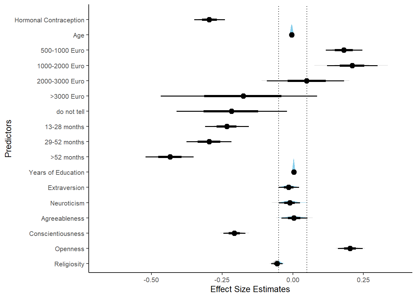
Effects of (In)Congruenct HC Use
Attractiveness of Partner
Model
Summary
##  Family: gaussian
##   Links: mu = identity; sigma = identity
## Formula: attractiveness_partner ~ contraception_hormonal * congruent_contraception
##    Data: data (Number of observations: 774)
##   Draws: 4 chains, each with iter = 2000; warmup = 1000; thin = 1;
##          total post-warmup draws = 4000
##
## Population-Level Effects:
##                                                    Estimate Est.Error l-90% CI u-90% CI Rhat Bulk_ESS
## Intercept                                              4.13      0.06     4.03     4.23 1.00     2377
## contraception_hormonalyes                              0.17      0.09     0.02     0.31 1.00     1982
## congruent_contraception1                               0.14      0.08     0.01     0.27 1.00     2228
## contraception_hormonalyes:congruent_contraception1    -0.13      0.11    -0.31     0.04 1.00     1877
##                                                    Tail_ESS
## Intercept                                              2715
## contraception_hormonalyes                              2296
## congruent_contraception1                               2605
## contraception_hormonalyes:congruent_contraception1     2380
##
## Family Specific Parameters:
##       Estimate Est.Error l-90% CI u-90% CI Rhat Bulk_ESS Tail_ESS
## sigma     0.74      0.02     0.71     0.77 1.00     2990     2773
##
## Draws were sampled using sampling(NUTS). For each parameter, Bulk_ESS
## and Tail_ESS are effective sample size measures, and Rhat is the potential
## scale reduction factor on split chains (at convergence, Rhat = 1).
Comparison with ROPE
plot(equivalence_test(m_congruency_atrr, range = c(-0.07, 0.07), ci = 0.90,
                      parameters = "contraception"))
## Possible multicollinearity between b_contraception_hormonalyes:congruent_contraception1 and b_contraception_hormonalyes (r = 0.79). This might lead to inappropriate results. See 'Details' in '?equivalence_test'.## Picking joint bandwidth of 0.0125## Warning: Removed 1197 rows containing non-finite values (stat_density_ridges).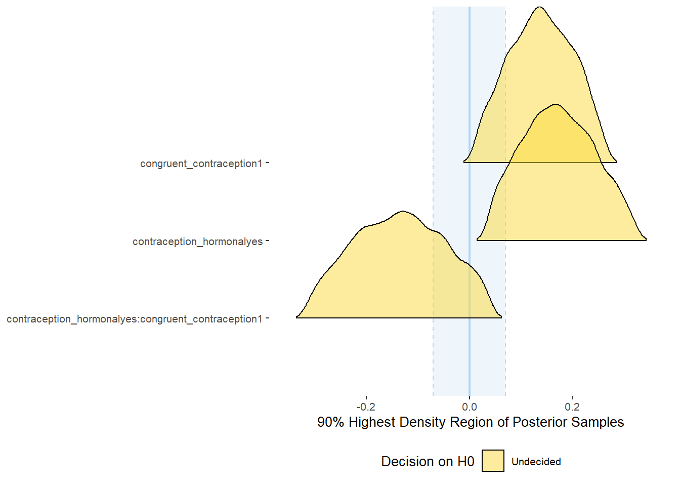
equivalence_test(m_congruency_atrr, range = c(-0.07, 0.07), ci = 0.90,
                      parameters = "contraception")
## Possible multicollinearity between b_contraception_hormonalyes:congruent_contraception1 and b_contraception_hormonalyes (r = 0.79). This might lead to inappropriate results. See 'Details' in '?equivalence_test'.## # A tibble: 3 x 10
## Parameter CI ROPE_low ROPE_high ROPE_Percentage ROPE_Equivalence HDI_low HDI_high Effects Component
## <chr> <dbl> <dbl> <dbl> <dbl> <chr> <dbl> <dbl> <chr> <chr>
## 1 b_contraceptio~ 0.9 -0.07 0.07 0.0711 Undecided 0.0377 0.322 fixed conditio~
## 2 b_congruent_co~ 0.9 -0.07 0.07 0.150 Undecided 0.0128 0.263 fixed conditio~
## 3 b_contraceptio~ 0.9 -0.07 0.07 0.256 Undecided -0.315 0.0417 fixed conditio~
Forest Plot for Effect Sizes
m_congruency_atrr %>%
  spread_draws(b_contraception_hormonalyes, b_congruent_contraception1,
               `b_contraception_hormonalyes:congruent_contraception1`) %>%
  pivot_longer(cols = c(b_contraception_hormonalyes, b_congruent_contraception1,
               `b_contraception_hormonalyes:congruent_contraception1`),
               names_to = "condition",
               values_to = "r_condition") %>%
  mutate(condition_mean = r_condition,
         group = ifelse(condition %contains% "ontraception",
                        "Contraception", NA),
         condition = ifelse(condition == "b_contraception_hormonalyes",
                        "Hormonal Contraception",
                     ifelse(condition == "b_congruent_contraception1",
                            "Congruent Contraception",
                     ifelse(condition == "b_contraception_hormonalyes:congruent_contraception1",
                            "Interaction Hormonal Contracpetion and Congruent Contraception",
                            condition))),
         condition = factor(condition, levels = rev(c("Hormonal Contraception",
                                            "Congruent Contraception",
                                            "Interaction Hormonal Contracpetion and Congruent Contraception")))) %>%
  ggplot(aes(y = condition,
             x = condition_mean,
             fill = stat(abs(x) < 0.07))) +
  stat_halfeye() +
  geom_vline(xintercept = c(-0.07, 0.07), linetype = "dotted") +
  apatheme +
  theme(legend.position = "none") +
  scale_fill_manual(values = c("gray80", "skyblue")) +
  labs(x = "Effect Size Estimates", y = "Predictors") +
  xlim (-0.6, 0.6)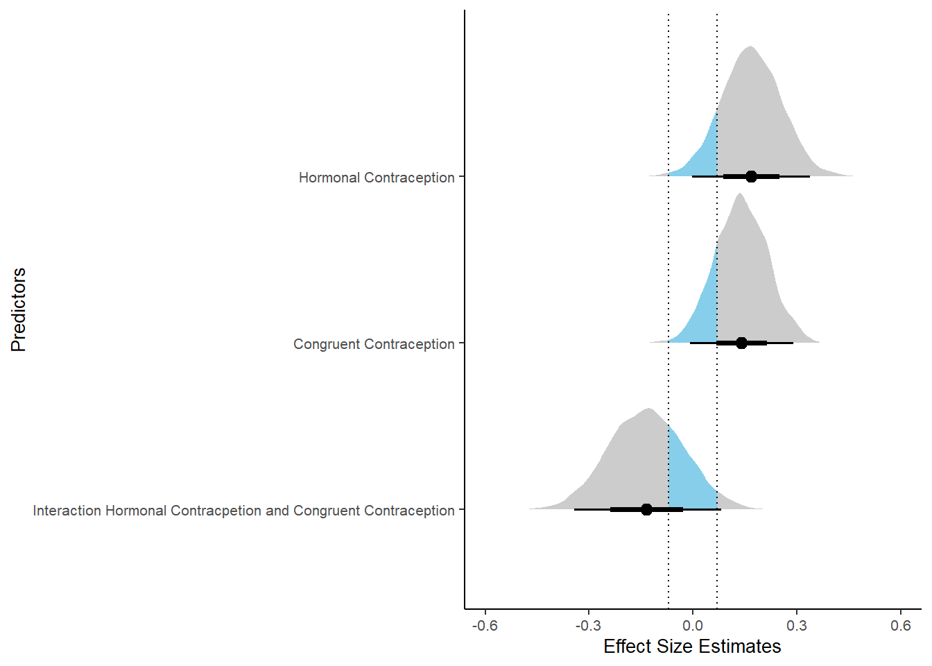
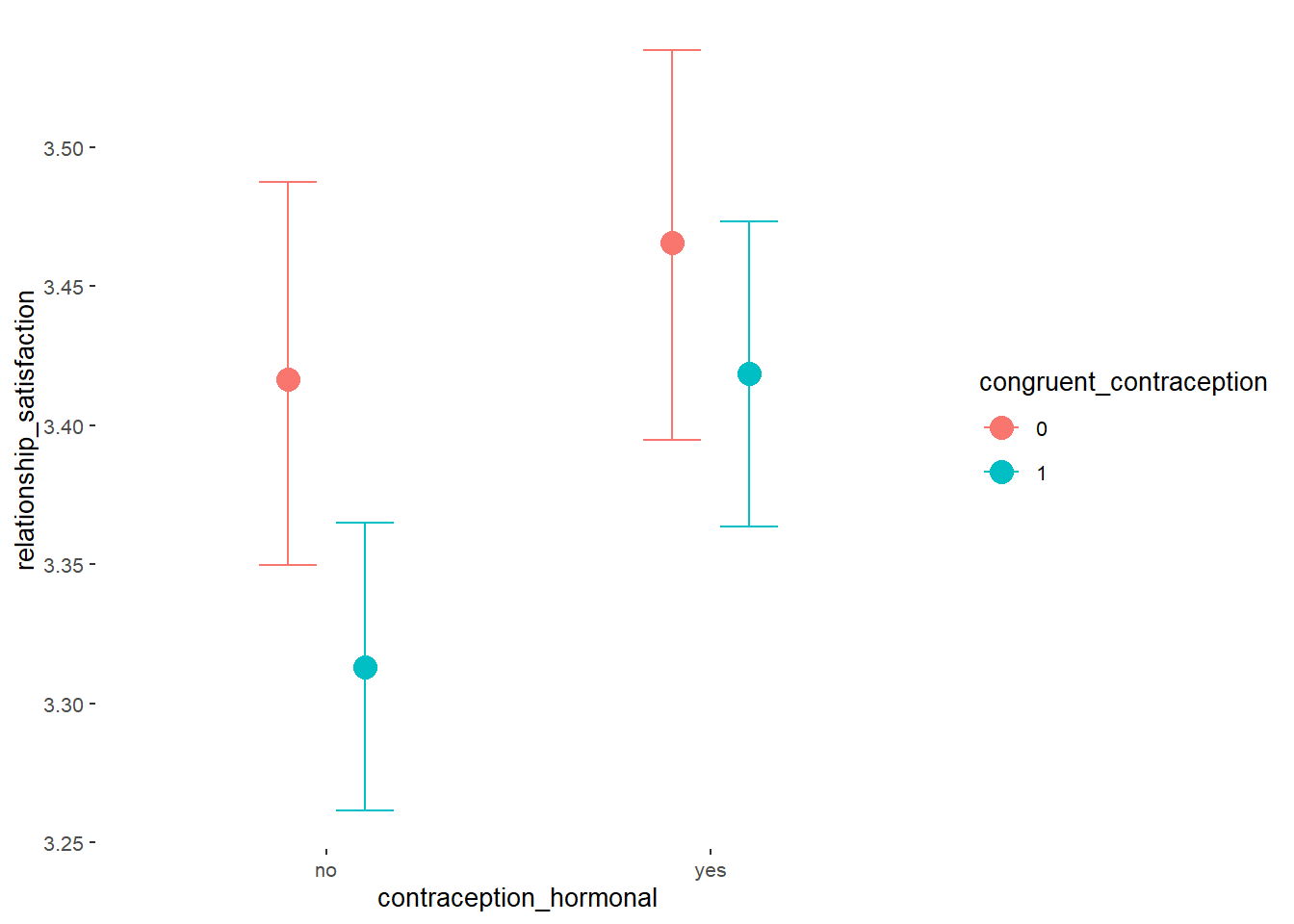
Relationship Satisfaction
Model
Summary
##  Family: gaussian
##   Links: mu = identity; sigma = identity
## Formula: relationship_satisfaction ~ contraception_hormonal * congruent_contraception
##    Data: data (Number of observations: 774)
##   Draws: 4 chains, each with iter = 2000; warmup = 1000; thin = 1;
##          total post-warmup draws = 4000
##
## Population-Level Effects:
##                                                    Estimate Est.Error l-90% CI u-90% CI Rhat Bulk_ESS
## Intercept                                              3.42      0.04     3.36     3.47 1.00     2107
## contraception_hormonalyes                              0.05      0.05    -0.03     0.13 1.00     1811
## congruent_contraception1                              -0.10      0.04    -0.18    -0.03 1.00     1922
## contraception_hormonalyes:congruent_contraception1     0.06      0.06    -0.05     0.16 1.00     1720
##                                                    Tail_ESS
## Intercept                                              2335
## contraception_hormonalyes                              2605
## congruent_contraception1                               2314
## contraception_hormonalyes:congruent_contraception1     2381
##
## Family Specific Parameters:
##       Estimate Est.Error l-90% CI u-90% CI Rhat Bulk_ESS Tail_ESS
## sigma     0.42      0.01     0.41     0.44 1.01     3232     2151
##
## Draws were sampled using sampling(NUTS). For each parameter, Bulk_ESS
## and Tail_ESS are effective sample size measures, and Rhat is the potential
## scale reduction factor on split chains (at convergence, Rhat = 1).
Comparison with ROPE
plot(equivalence_test(m_congruency_relsat, range = c(-0.04, 0.04), ci = 0.90,
                      parameters = "contraception"))
## Possible multicollinearity between b_contraception_hormonalyes:congruent_contraception1 and b_contraception_hormonalyes (r = 0.79), b_contraception_hormonalyes:congruent_contraception1 and b_congruent_contraception1 (r = 0.71). This might lead to inappropriate results. See 'Details' in '?equivalence_test'.## Picking joint bandwidth of 0.00737## Warning: Removed 1197 rows containing non-finite values (stat_density_ridges).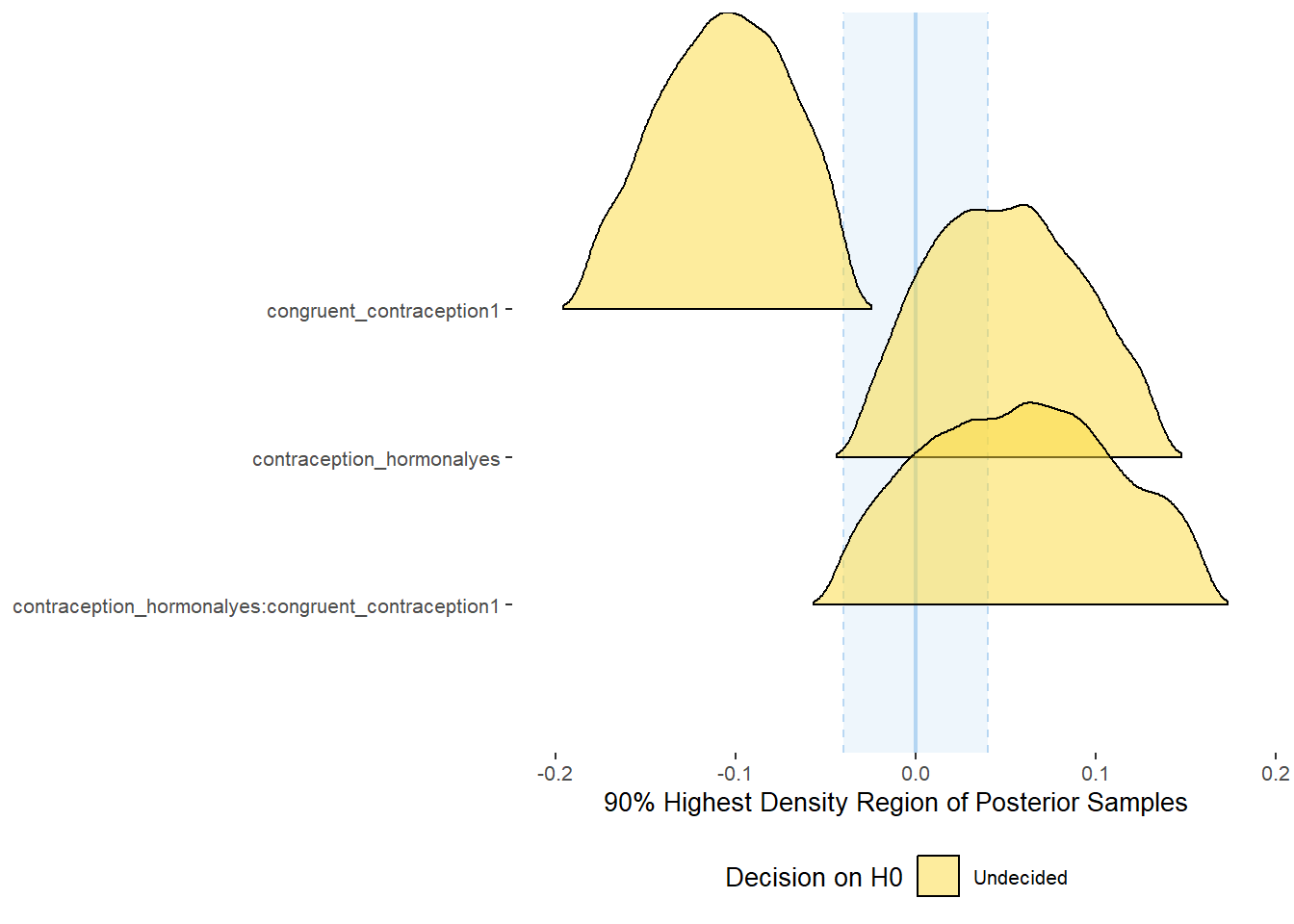
equivalence_test(m_congruency_relsat, range = c(-0.04, 0.04), ci = 0.90,
                      parameters = "contraception")
## Possible multicollinearity between b_contraception_hormonalyes:congruent_contraception1 and b_contraception_hormonalyes (r = 0.79), b_contraception_hormonalyes:congruent_contraception1 and b_congruent_contraception1 (r = 0.71). This might lead to inappropriate results. See 'Details' in '?equivalence_test'.## # A tibble: 3 x 10
## Parameter CI ROPE_low ROPE_high ROPE_Percentage ROPE_Equivalence HDI_low HDI_high Effects Component
## <chr> <dbl> <dbl> <dbl> <dbl> <chr> <dbl> <dbl> <chr> <chr>
## 1 b_contraceptio~ 0.9 -0.04 0.04 0.425 Undecided -0.0300 0.135 fixed conditio~
## 2 b_congruent_co~ 0.9 -0.04 0.04 0.00555 Undecided -0.183 -0.0386 fixed conditio~
## 3 b_contraceptio~ 0.9 -0.04 0.04 0.377 Undecided -0.0439 0.161 fixed conditio~
Forest Plot for Effect Sizes
m_congruency_relsat %>%
  spread_draws(b_contraception_hormonalyes, b_congruent_contraception1,
               `b_contraception_hormonalyes:congruent_contraception1`) %>%
  pivot_longer(cols = c(b_contraception_hormonalyes, b_congruent_contraception1,
               `b_contraception_hormonalyes:congruent_contraception1`),
               names_to = "condition",
               values_to = "r_condition") %>%
  mutate(condition_mean = r_condition,
         group = ifelse(condition %contains% "ontraception",
                        "Contraception", NA),
         condition = ifelse(condition == "b_contraception_hormonalyes",
                        "Hormonal Contraception",
                     ifelse(condition == "b_congruent_contraception1",
                            "Congruent Contraception",
                     ifelse(condition == "b_contraception_hormonalyes:congruent_contraception1",
                            "Interaction Hormonal Contracpetion and Congruent Contraception",
                            condition))),
         condition = factor(condition, levels = rev(c("Hormonal Contraception",
                                            "Congruent Contraception",
                                            "Interaction Hormonal Contracpetion and Congruent Contraception")))) %>%
  ggplot(aes(y = condition,
             x = condition_mean,
             fill = stat(abs(x) < 0.04))) +
  stat_halfeye() +
  geom_vline(xintercept = c(-0.04, 0.04), linetype = "dotted") +
  apatheme +
  theme(legend.position = "none") +
  scale_fill_manual(values = c("gray80", "skyblue")) +
  labs(x = "Effect Size Estimates", y = "Predictors") +
  xlim (-0.6, 0.6)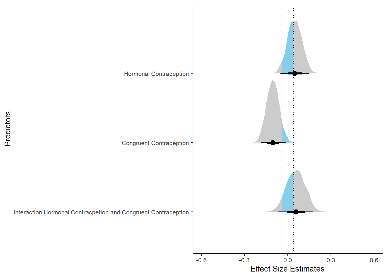
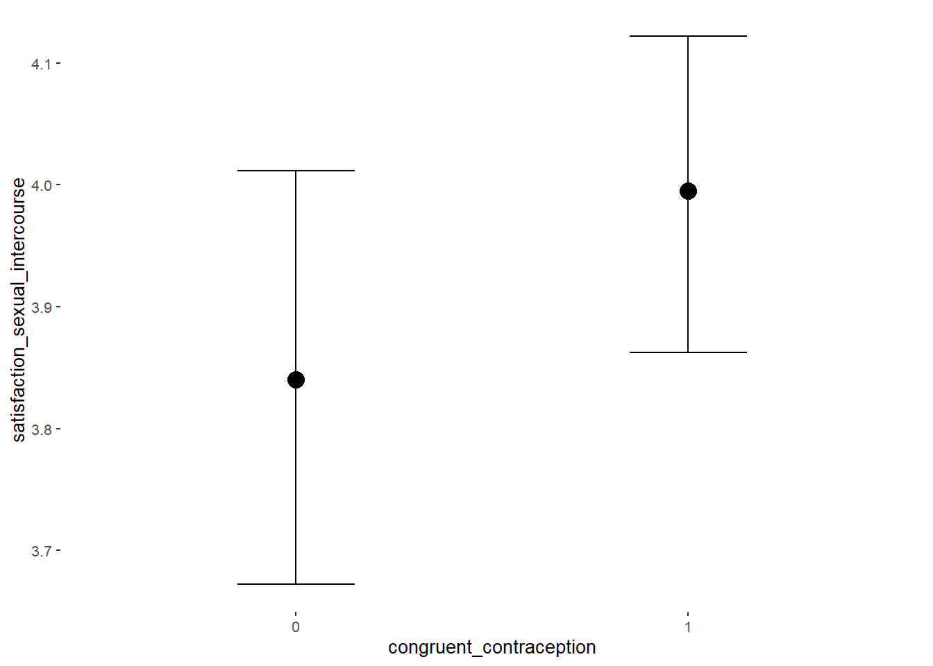
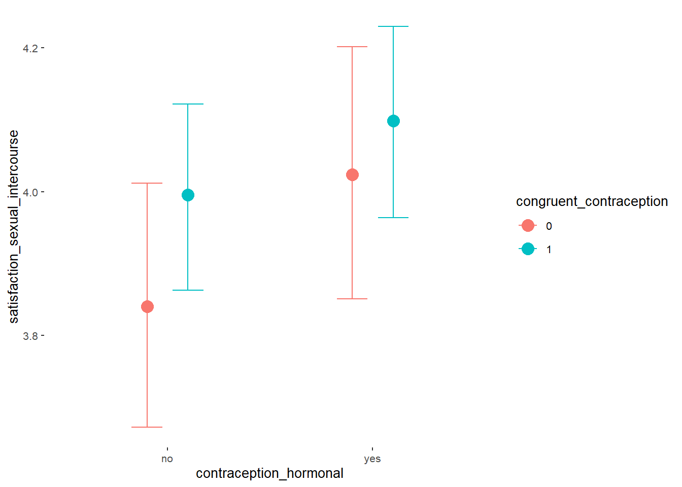
Sexual Satisfaction
Model
Summary
##  Family: gaussian
##   Links: mu = identity; sigma = identity
## Formula: satisfaction_sexual_intercourse ~ contraception_hormonal * congruent_contraception
##    Data: data (Number of observations: 774)
##   Draws: 4 chains, each with iter = 2000; warmup = 1000; thin = 1;
##          total post-warmup draws = 4000
##
## Population-Level Effects:
##                                                    Estimate Est.Error l-90% CI u-90% CI Rhat Bulk_ESS
## Intercept                                              3.84      0.09     3.70     3.98 1.00     1861
## contraception_hormonalyes                              0.18      0.12    -0.02     0.39 1.00     1693
## congruent_contraception1                               0.15      0.11    -0.03     0.33 1.00     1958
## contraception_hormonalyes:congruent_contraception1    -0.08      0.16    -0.33     0.19 1.00     1602
##                                                    Tail_ESS
## Intercept                                              2624
## contraception_hormonalyes                              2227
## congruent_contraception1                               2102
## contraception_hormonalyes:congruent_contraception1     2198
##
## Family Specific Parameters:
##       Estimate Est.Error l-90% CI u-90% CI Rhat Bulk_ESS Tail_ESS
## sigma     1.05      0.03     1.01     1.10 1.00     3579     2812
##
## Draws were sampled using sampling(NUTS). For each parameter, Bulk_ESS
## and Tail_ESS are effective sample size measures, and Rhat is the potential
## scale reduction factor on split chains (at convergence, Rhat = 1).
Comparison with ROPE
plot(equivalence_test(m_congruency_sexsat, range = c(-0.11, 0.11), ci = 0.90,
                      parameters = "contraception"))
## Possible multicollinearity between b_contraception_hormonalyes:congruent_contraception1 and b_contraception_hormonalyes (r = 0.8), b_contraception_hormonalyes:congruent_contraception1 and b_congruent_contraception1 (r = 0.7). This might lead to inappropriate results. See 'Details' in '?equivalence_test'.## Picking joint bandwidth of 0.018## Warning: Removed 1197 rows containing non-finite values (stat_density_ridges).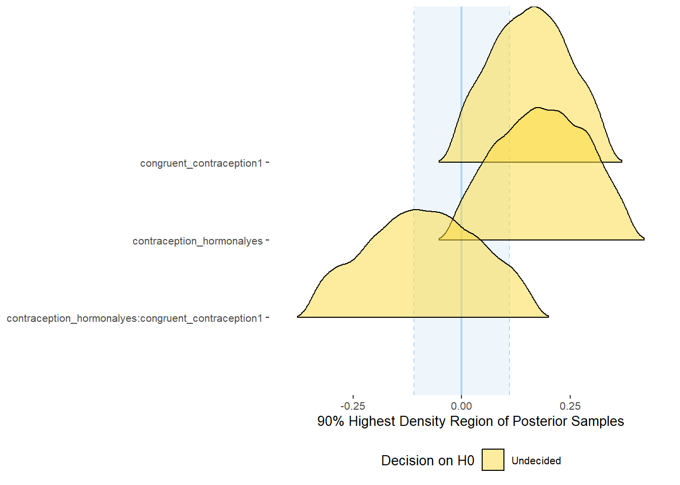
equivalence_test(m_congruency_sexsat, range = c(-0.11, 0.11), ci = 0.90,
                      parameters = "contraception")
## Possible multicollinearity between b_contraception_hormonalyes:congruent_contraception1 and b_contraception_hormonalyes (r = 0.8), b_contraception_hormonalyes:congruent_contraception1 and b_congruent_contraception1 (r = 0.7). This might lead to inappropriate results. See 'Details' in '?equivalence_test'.## # A tibble: 3 x 10
## Parameter CI ROPE_low ROPE_high ROPE_Percentage ROPE_Equivalence HDI_low HDI_high Effects Component
## <chr> <dbl> <dbl> <dbl> <dbl> <chr> <dbl> <dbl> <chr> <chr>
## 1 b_contraceptio~ 0.9 -0.11 0.11 0.249 Undecided -0.0184 0.390 fixed conditio~
## 2 b_congruent_co~ 0.9 -0.11 0.11 0.313 Undecided -0.0187 0.335 fixed conditio~
## 3 b_contraceptio~ 0.9 -0.11 0.11 0.500 Undecided -0.347 0.171 fixed conditio~
Forest Plot for Effect Sizes
m_congruency_sexsat %>%
  spread_draws(b_contraception_hormonalyes, b_congruent_contraception1,
               `b_contraception_hormonalyes:congruent_contraception1`) %>%
  pivot_longer(cols = c(b_contraception_hormonalyes, b_congruent_contraception1,
               `b_contraception_hormonalyes:congruent_contraception1`),
               names_to = "condition",
               values_to = "r_condition") %>%
  mutate(condition_mean = r_condition,
         group = ifelse(condition %contains% "ontraception",
                        "Contraception", NA),
         condition = ifelse(condition == "b_contraception_hormonalyes",
                        "Hormonal Contraception",
                     ifelse(condition == "b_congruent_contraception1",
                            "Congruent Contraception",
                     ifelse(condition == "b_contraception_hormonalyes:congruent_contraception1",
                            "Interaction Hormonal Contracpetion and Congruent Contraception",
                            condition))),
         condition = factor(condition, levels = rev(c("Hormonal Contraception",
                                            "Congruent Contraception",
                                            "Interaction Hormonal Contracpetion and Congruent Contraception")))) %>%
  ggplot(aes(y = condition,
             x = condition_mean,
             fill = stat(abs(x) < 0.11))) +
  stat_halfeye() +
  geom_vline(xintercept = c(-0.11, 0.11), linetype = "dotted") +
  apatheme +
  theme(legend.position = "none") +
  scale_fill_manual(values = c("gray80", "skyblue")) +
  labs(x = "Effect Size Estimates", y = "Predictors") +
  xlim (-0.6, 0.6)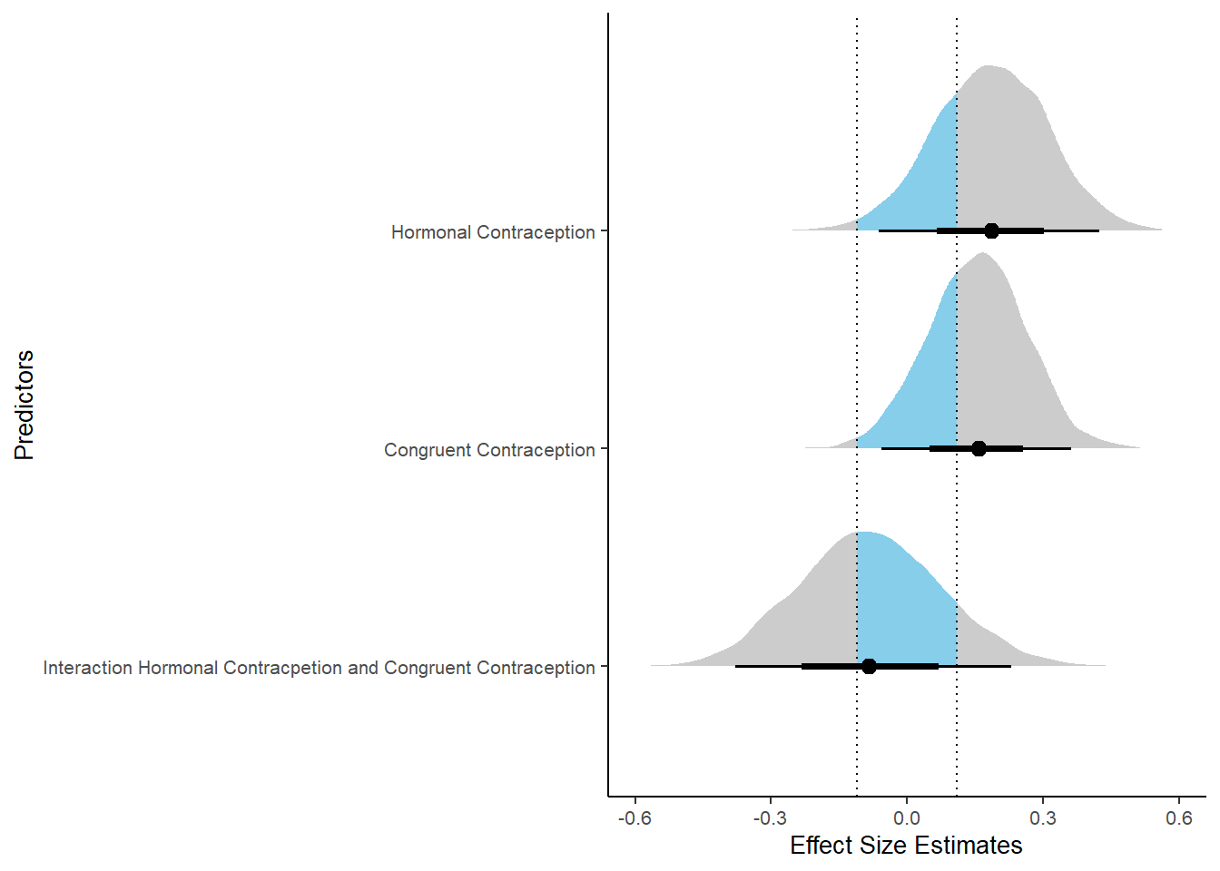
Libido
Model
Summary
##  Family: gaussian
##   Links: mu = identity; sigma = identity
## Formula: diary_libido_mean ~ contraception_hormonal * congruent_contraception
##    Data: data (Number of observations: 632)
##   Draws: 4 chains, each with iter = 2000; warmup = 1000; thin = 1;
##          total post-warmup draws = 4000
##
## Population-Level Effects:
##                                                    Estimate Est.Error l-90% CI u-90% CI Rhat Bulk_ESS
## Intercept                                              1.24      0.05     1.16     1.32 1.00     2486
## contraception_hormonalyes                             -0.00      0.07    -0.12     0.12 1.00     2076
## congruent_contraception1                               0.08      0.06    -0.02     0.18 1.00     2440
## contraception_hormonalyes:congruent_contraception1    -0.03      0.09    -0.18     0.12 1.00     2006
##                                                    Tail_ESS
## Intercept                                              2557
## contraception_hormonalyes                              2537
## congruent_contraception1                               2560
## contraception_hormonalyes:congruent_contraception1     2333
##
## Family Specific Parameters:
##       Estimate Est.Error l-90% CI u-90% CI Rhat Bulk_ESS Tail_ESS
## sigma     0.55      0.02     0.52     0.57 1.00     2952     2594
##
## Draws were sampled using sampling(NUTS). For each parameter, Bulk_ESS
## and Tail_ESS are effective sample size measures, and Rhat is the potential
## scale reduction factor on split chains (at convergence, Rhat = 1).
Comparison with ROPE
plot(equivalence_test(m_congruency_libido, range = c(-0.06, 0.06), ci = 0.90,
                      parameters = "contraception"))
## Possible multicollinearity between b_contraception_hormonalyes:congruent_contraception1 and b_contraception_hormonalyes (r = 0.81). This might lead to inappropriate results. See 'Details' in '?equivalence_test'.## Picking joint bandwidth of 0.0104## Warning: Removed 1197 rows containing non-finite values (stat_density_ridges).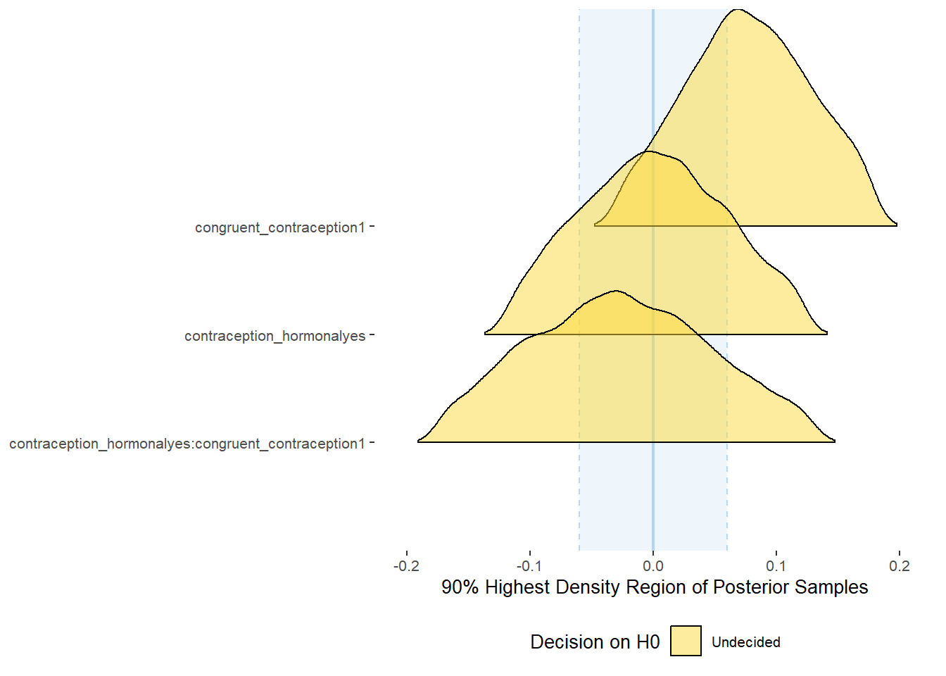
equivalence_test(m_congruency_libido, range = c(-0.06, 0.06), ci = 0.90,
                      parameters = "contraception")
## Possible multicollinearity between b_contraception_hormonalyes:congruent_contraception1 and b_contraception_hormonalyes (r = 0.81). This might lead to inappropriate results. See 'Details' in '?equivalence_test'.## # A tibble: 3 x 10
## Parameter CI ROPE_low ROPE_high ROPE_Percentage ROPE_Equivalence HDI_low HDI_high Effects Component
## <chr> <dbl> <dbl> <dbl> <dbl> <chr> <dbl> <dbl> <chr> <chr>
## 1 b_contraceptio~ 0.9 -0.06 0.06 0.658 Undecided -0.119 0.122 fixed conditio~
## 2 b_congruent_co~ 0.9 -0.06 0.06 0.373 Undecided -0.0286 0.178 fixed conditio~
## 3 b_contraceptio~ 0.9 -0.06 0.06 0.534 Undecided -0.174 0.131 fixed conditio~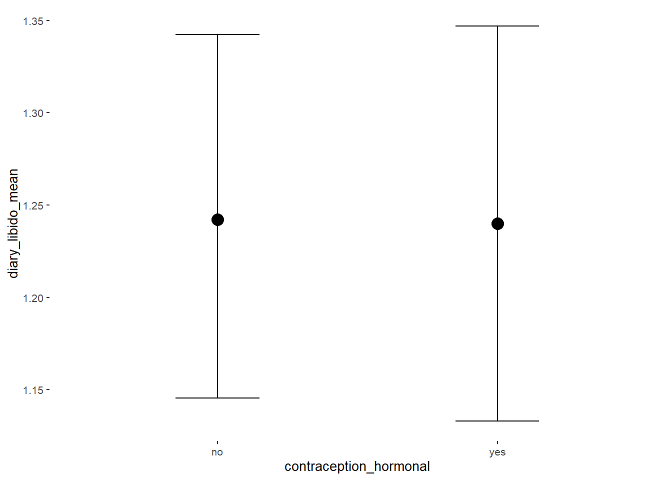
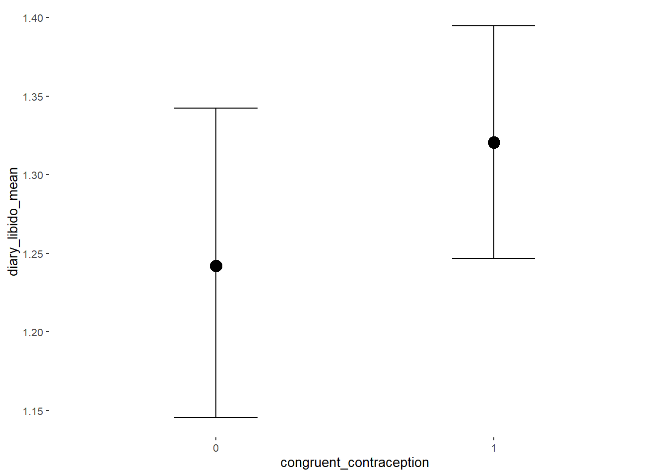
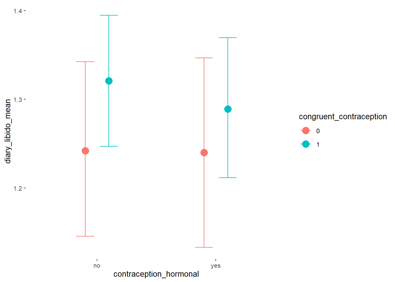
Forest Plot for Effect Sizes
m_congruency_libido %>%
  spread_draws(b_contraception_hormonalyes, b_congruent_contraception1,
               `b_contraception_hormonalyes:congruent_contraception1`) %>%
  pivot_longer(cols = c(b_contraception_hormonalyes, b_congruent_contraception1,
               `b_contraception_hormonalyes:congruent_contraception1`),
               names_to = "condition",
               values_to = "r_condition") %>%
  mutate(condition_mean = r_condition,
         group = ifelse(condition %contains% "ontraception",
                        "Contraception", NA),
         condition = ifelse(condition == "b_contraception_hormonalyes",
                        "Hormonal Contraception",
                     ifelse(condition == "b_congruent_contraception1",
                            "Congruent Contraception",
                     ifelse(condition == "b_contraception_hormonalyes:congruent_contraception1",
                            "Interaction Hormonal Contracpetion and Congruent Contraception",
                            condition))),
         condition = factor(condition, levels = rev(c("Hormonal Contraception",
                                            "Congruent Contraception",
                                            "Interaction Hormonal Contracpetion and Congruent Contraception")))) %>%
  ggplot(aes(y = condition,
             x = condition_mean,
             fill = stat(abs(x) < 0.06))) +
  stat_halfeye() +
  geom_vline(xintercept = c(-0.06, 0.06), linetype = "dotted") +
  apatheme +
  theme(legend.position = "none") +
  scale_fill_manual(values = c("gray80", "skyblue")) +
  labs(x = "Effect Size Estimates", y = "Predictors") +
  xlim (-0.6, 0.6)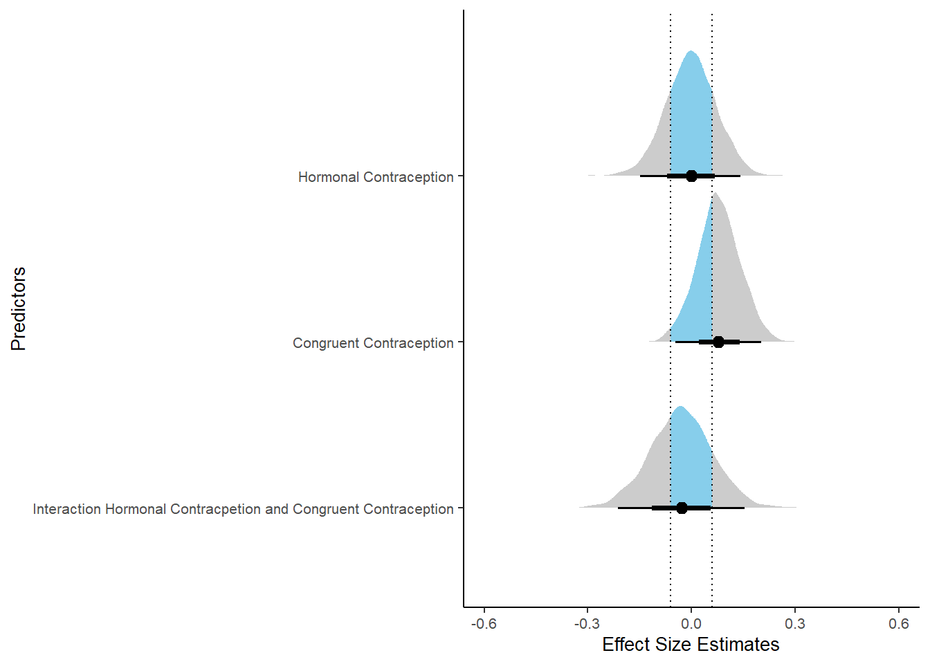
Sexual Frequency (Penetrative Intercourse)
Model
m_congruency_sexfreqpen = brm(diary_sex_active_sex_sum ~ offset(log(number_of_days)) +
                     contraception_hormonal * congruent_contraception,
                data = data, family = poisson(),
                file = "m_congruency_sexfreqpen")
## Warning: Rows containing NAs were excluded from the model.## Compiling Stan program...## Start sampling##
## SAMPLING FOR MODEL 'c63cc6f90adde557ca52c07be9ae7367' NOW (CHAIN 1).
## Chain 1:
## Chain 1: Gradient evaluation took 0 seconds
## Chain 1: 1000 transitions using 10 leapfrog steps per transition would take 0 seconds.
## Chain 1: Adjust your expectations accordingly!
## Chain 1:
## Chain 1:
## Chain 1: Iteration: 1 / 2000 [ 0%] (Warmup)
## Chain 1: Iteration: 200 / 2000 [ 10%] (Warmup)
## Chain 1: Iteration: 400 / 2000 [ 20%] (Warmup)
## Chain 1: Iteration: 600 / 2000 [ 30%] (Warmup)
## Chain 1: Iteration: 800 / 2000 [ 40%] (Warmup)
## Chain 1: Iteration: 1000 / 2000 [ 50%] (Warmup)
## Chain 1: Iteration: 1001 / 2000 [ 50%] (Sampling)
## Chain 1: Iteration: 1200 / 2000 [ 60%] (Sampling)
## Chain 1: Iteration: 1400 / 2000 [ 70%] (Sampling)
## Chain 1: Iteration: 1600 / 2000 [ 80%] (Sampling)
## Chain 1: Iteration: 1800 / 2000 [ 90%] (Sampling)
## Chain 1: Iteration: 2000 / 2000 [100%] (Sampling)
## Chain 1:
## Chain 1: Elapsed Time: 0.933 seconds (Warm-up)
## Chain 1: 0.911 seconds (Sampling)
## Chain 1: 1.844 seconds (Total)
## Chain 1:
##
## SAMPLING FOR MODEL 'c63cc6f90adde557ca52c07be9ae7367' NOW (CHAIN 2).
## Chain 2:
## Chain 2: Gradient evaluation took 0 seconds
## Chain 2: 1000 transitions using 10 leapfrog steps per transition would take 0 seconds.
## Chain 2: Adjust your expectations accordingly!
## Chain 2:
## Chain 2:
## Chain 2: Iteration: 1 / 2000 [ 0%] (Warmup)
## Chain 2: Iteration: 200 / 2000 [ 10%] (Warmup)
## Chain 2: Iteration: 400 / 2000 [ 20%] (Warmup)
## Chain 2: Iteration: 600 / 2000 [ 30%] (Warmup)
## Chain 2: Iteration: 800 / 2000 [ 40%] (Warmup)
## Chain 2: Iteration: 1000 / 2000 [ 50%] (Warmup)
## Chain 2: Iteration: 1001 / 2000 [ 50%] (Sampling)
## Chain 2: Iteration: 1200 / 2000 [ 60%] (Sampling)
## Chain 2: Iteration: 1400 / 2000 [ 70%] (Sampling)
## Chain 2: Iteration: 1600 / 2000 [ 80%] (Sampling)
## Chain 2: Iteration: 1800 / 2000 [ 90%] (Sampling)
## Chain 2: Iteration: 2000 / 2000 [100%] (Sampling)
## Chain 2:
## Chain 2: Elapsed Time: 0.912 seconds (Warm-up)
## Chain 2: 0.94 seconds (Sampling)
## Chain 2: 1.852 seconds (Total)
## Chain 2:
##
## SAMPLING FOR MODEL 'c63cc6f90adde557ca52c07be9ae7367' NOW (CHAIN 3).
## Chain 3:
## Chain 3: Gradient evaluation took 0 seconds
## Chain 3: 1000 transitions using 10 leapfrog steps per transition would take 0 seconds.
## Chain 3: Adjust your expectations accordingly!
## Chain 3:
## Chain 3:
## Chain 3: Iteration: 1 / 2000 [ 0%] (Warmup)
## Chain 3: Iteration: 200 / 2000 [ 10%] (Warmup)
## Chain 3: Iteration: 400 / 2000 [ 20%] (Warmup)
## Chain 3: Iteration: 600 / 2000 [ 30%] (Warmup)
## Chain 3: Iteration: 800 / 2000 [ 40%] (Warmup)
## Chain 3: Iteration: 1000 / 2000 [ 50%] (Warmup)
## Chain 3: Iteration: 1001 / 2000 [ 50%] (Sampling)
## Chain 3: Iteration: 1200 / 2000 [ 60%] (Sampling)
## Chain 3: Iteration: 1400 / 2000 [ 70%] (Sampling)
## Chain 3: Iteration: 1600 / 2000 [ 80%] (Sampling)
## Chain 3: Iteration: 1800 / 2000 [ 90%] (Sampling)
## Chain 3: Iteration: 2000 / 2000 [100%] (Sampling)
## Chain 3:
## Chain 3: Elapsed Time: 0.99 seconds (Warm-up)
## Chain 3: 1.03 seconds (Sampling)
## Chain 3: 2.02 seconds (Total)
## Chain 3:
##
## SAMPLING FOR MODEL 'c63cc6f90adde557ca52c07be9ae7367' NOW (CHAIN 4).
## Chain 4:
## Chain 4: Gradient evaluation took 0 seconds
## Chain 4: 1000 transitions using 10 leapfrog steps per transition would take 0 seconds.
## Chain 4: Adjust your expectations accordingly!
## Chain 4:
## Chain 4:
## Chain 4: Iteration: 1 / 2000 [ 0%] (Warmup)
## Chain 4: Iteration: 200 / 2000 [ 10%] (Warmup)
## Chain 4: Iteration: 400 / 2000 [ 20%] (Warmup)
## Chain 4: Iteration: 600 / 2000 [ 30%] (Warmup)
## Chain 4: Iteration: 800 / 2000 [ 40%] (Warmup)
## Chain 4: Iteration: 1000 / 2000 [ 50%] (Warmup)
## Chain 4: Iteration: 1001 / 2000 [ 50%] (Sampling)
## Chain 4: Iteration: 1200 / 2000 [ 60%] (Sampling)
## Chain 4: Iteration: 1400 / 2000 [ 70%] (Sampling)
## Chain 4: Iteration: 1600 / 2000 [ 80%] (Sampling)
## Chain 4: Iteration: 1800 / 2000 [ 90%] (Sampling)
## Chain 4: Iteration: 2000 / 2000 [100%] (Sampling)
## Chain 4:
## Chain 4: Elapsed Time: 0.91 seconds (Warm-up)
## Chain 4: 0.96 seconds (Sampling)
## Chain 4: 1.87 seconds (Total)
## Chain 4:Summary
##  Family: poisson
##   Links: mu = log
## Formula: diary_sex_active_sex_sum ~ offset(log(number_of_days)) + contraception_hormonal * congruent_contraception
##    Data: data (Number of observations: 622)
##   Draws: 4 chains, each with iter = 2000; warmup = 1000; thin = 1;
##          total post-warmup draws = 4000
##
## Population-Level Effects:
##                                                    Estimate Est.Error l-90% CI u-90% CI Rhat Bulk_ESS
## Intercept                                             -1.87      0.03    -1.93    -1.82 1.00     1883
## contraception_hormonalyes                              0.20      0.05     0.12     0.27 1.00     1682
## congruent_contraception1                               0.09      0.04     0.02     0.15 1.00     1774
## contraception_hormonalyes:congruent_contraception1    -0.09      0.06    -0.18     0.01 1.00     1535
##                                                    Tail_ESS
## Intercept                                              2465
## contraception_hormonalyes                              2151
## congruent_contraception1                               2486
## contraception_hormonalyes:congruent_contraception1     1891
##
## Draws were sampled using sampling(NUTS). For each parameter, Bulk_ESS
## and Tail_ESS are effective sample size measures, and Rhat is the potential
## scale reduction factor on split chains (at convergence, Rhat = 1).
Comparison with ROPE
plot(equivalence_test(m_congruency_sexfreqpen, range = c(-0.05, 0.05), ci = 0.90,
                      parameters = "contraception"))
## Possible multicollinearity between b_contraception_hormonalyes:congruent_contraception1 and b_contraception_hormonalyes (r = 0.81), b_contraception_hormonalyes:congruent_contraception1 and b_congruent_contraception1 (r = 0.71). This might lead to inappropriate results. See 'Details' in '?equivalence_test'.## Picking joint bandwidth of 0.00654## Warning: Removed 1197 rows containing non-finite values (stat_density_ridges).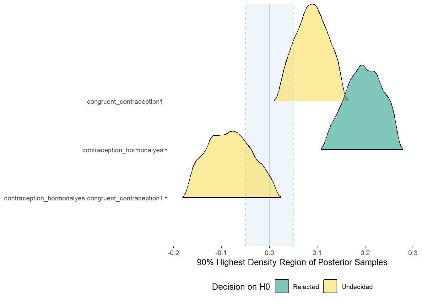
equivalence_test(m_congruency_sexfreqpen, range = c(-0.05, 0.05), ci = 0.90,
                      parameters = "contraception")
## Possible multicollinearity between b_contraception_hormonalyes:congruent_contraception1 and b_contraception_hormonalyes (r = 0.81), b_contraception_hormonalyes:congruent_contraception1 and b_congruent_contraception1 (r = 0.71). This might lead to inappropriate results. See 'Details' in '?equivalence_test'.## # A tibble: 3 x 10
## Parameter CI ROPE_low ROPE_high ROPE_Percentage ROPE_Equivalence HDI_low HDI_high Effects Component
## <chr> <dbl> <dbl> <dbl> <dbl> <chr> <dbl> <dbl> <chr> <chr>
## 1 b_contraceptio~ 0.9 -0.05 0.05 0 Rejected 0.119 0.266 fixed conditio~
## 2 b_congruent_co~ 0.9 -0.05 0.05 0.134 Undecided 0.0225 0.152 fixed conditio~
## 3 b_contraceptio~ 0.9 -0.05 0.05 0.253 Undecided -0.170 0.0126 fixed conditio~Plots
conditional_effects(m_congruency_sexfreqpen,
                    effects = "contraception_hormonal:congruent_contraception",
                    conditions = data.frame(number_of_days = 1))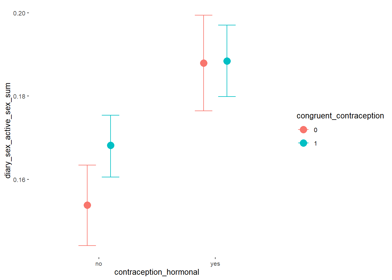
Forest Plot for Effect Sizes
m_congruency_sexfreqpen %>%
  spread_draws(b_contraception_hormonalyes, b_congruent_contraception1,
               `b_contraception_hormonalyes:congruent_contraception1`) %>%
  pivot_longer(cols = c(b_contraception_hormonalyes, b_congruent_contraception1,
               `b_contraception_hormonalyes:congruent_contraception1`),
               names_to = "condition",
               values_to = "r_condition") %>%
  mutate(condition_mean = r_condition,
         group = ifelse(condition %contains% "ontraception",
                        "Contraception", NA),
         condition = ifelse(condition == "b_contraception_hormonalyes",
                        "Hormonal Contraception",
                     ifelse(condition == "b_congruent_contraception1",
                            "Congruent Contraception",
                     ifelse(condition == "b_contraception_hormonalyes:congruent_contraception1",
                            "Interaction Hormonal Contracpetion and Congruent Contraception",
                            condition))),
         condition = factor(condition, levels = rev(c("Hormonal Contraception",
                                            "Congruent Contraception",
                                            "Interaction Hormonal Contracpetion and Congruent Contraception")))) %>%
  ggplot(aes(y = condition,
             x = condition_mean,
             fill = stat(abs(x) < 0.05))) +
  stat_halfeye() +
  geom_vline(xintercept = c(-0.05, 0.051), linetype = "dotted") +
  apatheme +
  theme(legend.position = "none") +
  scale_fill_manual(values = c("gray80", "skyblue")) +
  labs(x = "Effect Size Estimates", y = "Predictors")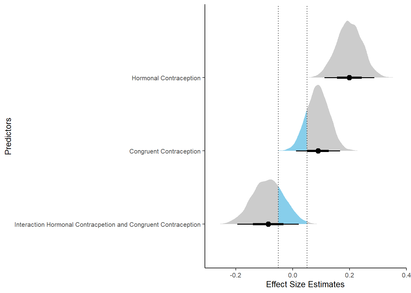
Masturbation Frequency
Model
Summary
##  Family: poisson
##   Links: mu = log
## Formula: diary_masturbation_sum ~ offset(log(number_of_days)) + contraception_hormonal * congruent_contraception
##    Data: data (Number of observations: 622)
##   Draws: 4 chains, each with iter = 2000; warmup = 1000; thin = 1;
##          total post-warmup draws = 4000
##
## Population-Level Effects:
##                                                    Estimate Est.Error l-90% CI u-90% CI Rhat Bulk_ESS
## Intercept                                             -2.09      0.04    -2.15    -2.03 1.00     2289
## contraception_hormonalyes                             -0.37      0.06    -0.46    -0.27 1.00     1814
## congruent_contraception1                               0.11      0.04     0.04     0.18 1.00     2096
## contraception_hormonalyes:congruent_contraception1     0.01      0.07    -0.10     0.13 1.00     1727
##                                                    Tail_ESS
## Intercept                                              2730
## contraception_hormonalyes                              2328
## congruent_contraception1                               2512
## contraception_hormonalyes:congruent_contraception1     2162
##
## Draws were sampled using sampling(NUTS). For each parameter, Bulk_ESS
## and Tail_ESS are effective sample size measures, and Rhat is the potential
## scale reduction factor on split chains (at convergence, Rhat = 1).
Comparison with ROPE
plot(equivalence_test(m_congruency_masfreq, range = c(-0.05, 0.05), ci = 0.90,
                      parameters = "contraception"))
## Possible multicollinearity between b_contraception_hormonalyes:congruent_contraception1 and b_contraception_hormonalyes (r = 0.82). This might lead to inappropriate results. See 'Details' in '?equivalence_test'.## Picking joint bandwidth of 0.00789## Warning: Removed 1197 rows containing non-finite values (stat_density_ridges).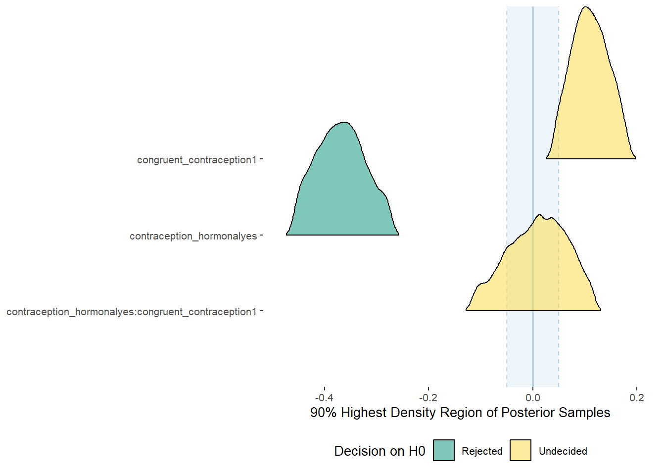
equivalence_test(m_congruency_masfreq, range = c(-0.05, 0.05), ci = 0.90,
                      parameters = "contraception")
## Possible multicollinearity between b_contraception_hormonalyes:congruent_contraception1 and b_contraception_hormonalyes (r = 0.82). This might lead to inappropriate results. See 'Details' in '?equivalence_test'.## # A tibble: 3 x 10
## Parameter CI ROPE_low ROPE_high ROPE_Percentage ROPE_Equivalence HDI_low HDI_high Effects Component
## <chr> <dbl> <dbl> <dbl> <dbl> <chr> <dbl> <dbl> <chr> <chr>
## 1 b_contraceptio~ 0.9 -0.05 0.05 0 Rejected -0.460 -0.271 fixed conditio~
## 2 b_congruent_co~ 0.9 -0.05 0.05 0.0339 Undecided 0.0416 0.183 fixed conditio~
## 3 b_contraceptio~ 0.9 -0.05 0.05 0.571 Undecided -0.117 0.118 fixed conditio~Plots
conditional_effects(m_congruency_masfreq,
                    effects = "contraception_hormonal:congruent_contraception",
                    conditions = data.frame(number_of_days = 1))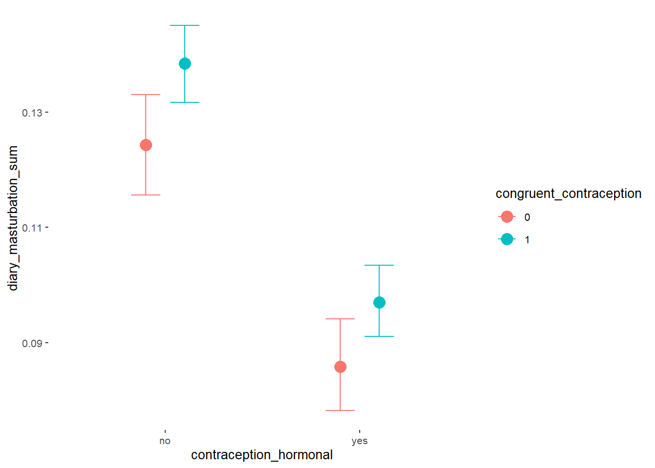
Forest Plot for Effect Sizes
m_congruency_masfreq %>%
spread_draws(b_contraception_hormonalyes, b_congruent_contraception1,
               `b_contraception_hormonalyes:congruent_contraception1`) %>%
  pivot_longer(cols = c(b_contraception_hormonalyes, b_congruent_contraception1,
               `b_contraception_hormonalyes:congruent_contraception1`),
               names_to = "condition",
               values_to = "r_condition") %>%
  mutate(condition_mean = r_condition,
         group = ifelse(condition %contains% "ontraception",
                        "Contraception", NA),
         condition = ifelse(condition == "b_contraception_hormonalyes",
                        "Hormonal Contraception",
                     ifelse(condition == "b_congruent_contraception1",
                            "Congruent Contraception",
                     ifelse(condition == "b_contraception_hormonalyes:congruent_contraception1",
                            "Interaction Hormonal Contracpetion and Congruent Contraception",
                            condition))),
         condition = factor(condition, levels = rev(c("Hormonal Contraception",
                                            "Congruent Contraception",
                                            "Interaction Hormonal Contracpetion and Congruent Contraception")))) %>%
  ggplot(aes(y = condition,
             x = condition_mean,
             fill = stat(abs(x) < 0.05))) +
  stat_halfeye() +
  geom_vline(xintercept = c(-0.05, 0.05), linetype = "dotted") +
  apatheme +
  theme(legend.position = "none") +
  scale_fill_manual(values = c("gray80", "skyblue")) +
  labs(x = "Effect Size Estimates", y = "Predictors")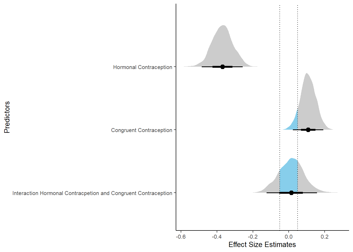
Controlled Models: Effects of (In)Congruenct HC Use
Attractiveness of Partner
Model
m_congruency_atrr_controlled = brm(attractiveness_partner ~
                          contraception_hormonal * congruent_contraception +
                             age + net_income + relationship_duration_factor +
                              education_years +
                              bfi_extra + bfi_neuro + bfi_agree + bfi_consc + bfi_open +
                              religiosity,
                data = data, family = gaussian(),
                file = "m_congruency_atrr_controlled")
Summary
##  Family: gaussian
##   Links: mu = identity; sigma = identity
## Formula: attractiveness_partner ~ contraception_hormonal * congruent_contraception + age + net_income + relationship_duration_factor + education_years + bfi_extra + bfi_neuro + bfi_agree + bfi_consc + bfi_open + religiosity
##    Data: data (Number of observations: 774)
##   Draws: 4 chains, each with iter = 2000; warmup = 1000; thin = 1;
##          total post-warmup draws = 4000
##
## Population-Level Effects:
##                                                        Estimate Est.Error l-90% CI u-90% CI Rhat Bulk_ESS
## Intercept                                                  3.21      0.37     2.59     3.80 1.00     4841
## contraception_hormonalyes                                  0.14      0.09    -0.01     0.29 1.00     3434
## congruent_contraception1                                   0.10      0.08    -0.03     0.23 1.00     3261
## age                                                       -0.00      0.01    -0.01     0.01 1.00     4709
## net_incomeeuro_500_1000                                    0.05      0.07    -0.07     0.16 1.00     3857
## net_incomeeuro_1000_2000                                   0.15      0.09     0.01     0.30 1.00     3699
## net_incomeeuro_2000_3000                                   0.19      0.12    -0.02     0.39 1.00     3928
## net_incomeeuro_gt_3000                                     0.18      0.21    -0.17     0.53 1.00     4157
## net_incomedont_tell                                       -0.00      0.18    -0.30     0.29 1.00     4275
## relationship_duration_factorPartnered_upto28months         0.12      0.08    -0.01     0.24 1.00     3956
## relationship_duration_factorPartnered_upto52months        -0.02      0.08    -0.15     0.11 1.00     3820
## relationship_duration_factorPartnered_morethan52months    -0.12      0.08    -0.26     0.02 1.00     3703
## education_years                                            0.01      0.01    -0.00     0.02 1.00     5536
## bfi_extra                                                  0.05      0.04    -0.01     0.11 1.00     4881
## bfi_neuro                                                  0.00      0.04    -0.06     0.07 1.00     4395
## bfi_agree                                                  0.10      0.05     0.03     0.18 1.00     4441
## bfi_consc                                                  0.03      0.04    -0.04     0.10 1.00     5647
## bfi_open                                                   0.06      0.05    -0.01     0.14 1.00     5430
## religiosity                                               -0.00      0.02    -0.03     0.03 1.00     4886
## contraception_hormonalyes:congruent_contraception1        -0.09      0.11    -0.28     0.09 1.00     3107
##                                                        Tail_ESS
## Intercept                                                  3175
## contraception_hormonalyes                                  2849
## congruent_contraception1                                   3133
## age                                                        3701
## net_incomeeuro_500_1000                                    3299
## net_incomeeuro_1000_2000                                   2937
## net_incomeeuro_2000_3000                                   3154
## net_incomeeuro_gt_3000                                     3170
## net_incomedont_tell                                        2884
## relationship_duration_factorPartnered_upto28months         3040
## relationship_duration_factorPartnered_upto52months         3060
## relationship_duration_factorPartnered_morethan52months     3061
## education_years                                            3286
## bfi_extra                                                  2971
## bfi_neuro                                                  3347
## bfi_agree                                                  3322
## bfi_consc                                                  3084
## bfi_open                                                   2807
## religiosity                                                3121
## contraception_hormonalyes:congruent_contraception1         2994
##
## Family Specific Parameters:
##       Estimate Est.Error l-90% CI u-90% CI Rhat Bulk_ESS Tail_ESS
## sigma     0.73      0.02     0.70     0.76 1.00     5358     2588
##
## Draws were sampled using sampling(NUTS). For each parameter, Bulk_ESS
## and Tail_ESS are effective sample size measures, and Rhat is the potential
## scale reduction factor on split chains (at convergence, Rhat = 1).
Comparison with ROPE
plot(equivalence_test(m_congruency_atrr_controlled, range = c(-0.07, 0.07), ci = 0.90,
                      parameters = "contraception"))
## Possible multicollinearity between b_contraception_hormonalyes:congruent_contraception1 and b_contraception_hormonalyes (r = 0.79), b_contraception_hormonalyes:congruent_contraception1 and b_congruent_contraception1 (r = 0.7). This might lead to inappropriate results. See 'Details' in '?equivalence_test'.## Picking joint bandwidth of 0.0132## Warning: Removed 1197 rows containing non-finite values (stat_density_ridges).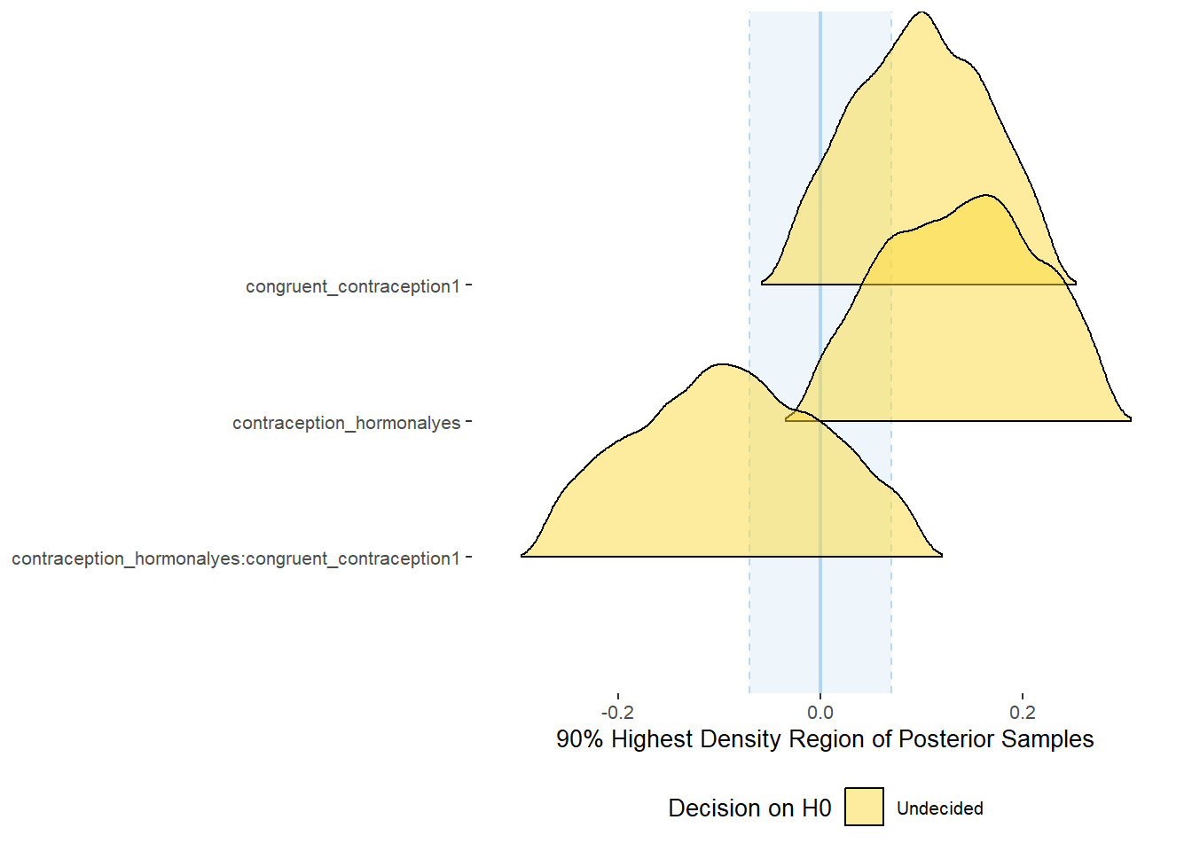
equivalence_test(m_congruency_atrr_controlled, range = c(-0.07, 0.07), ci = 0.90,
                      parameters = "contraception")
## Possible multicollinearity between b_contraception_hormonalyes:congruent_contraception1 and b_contraception_hormonalyes (r = 0.79), b_contraception_hormonalyes:congruent_contraception1 and b_congruent_contraception1 (r = 0.7). This might lead to inappropriate results. See 'Details' in '?equivalence_test'.## # A tibble: 3 x 10
## Parameter CI ROPE_low ROPE_high ROPE_Percentage ROPE_Equivalence HDI_low HDI_high Effects Component
## <chr> <dbl> <dbl> <dbl> <dbl> <chr> <dbl> <dbl> <chr> <chr>
## 1 b_contraceptio~ 0.9 -0.07 0.07 0.200 Undecided -0.0107 0.284 fixed conditio~
## 2 b_congruent_co~ 0.9 -0.07 0.07 0.340 Undecided -0.0350 0.228 fixed conditio~
## 3 b_contraceptio~ 0.9 -0.07 0.07 0.383 Undecided -0.274 0.0992 fixed conditio~
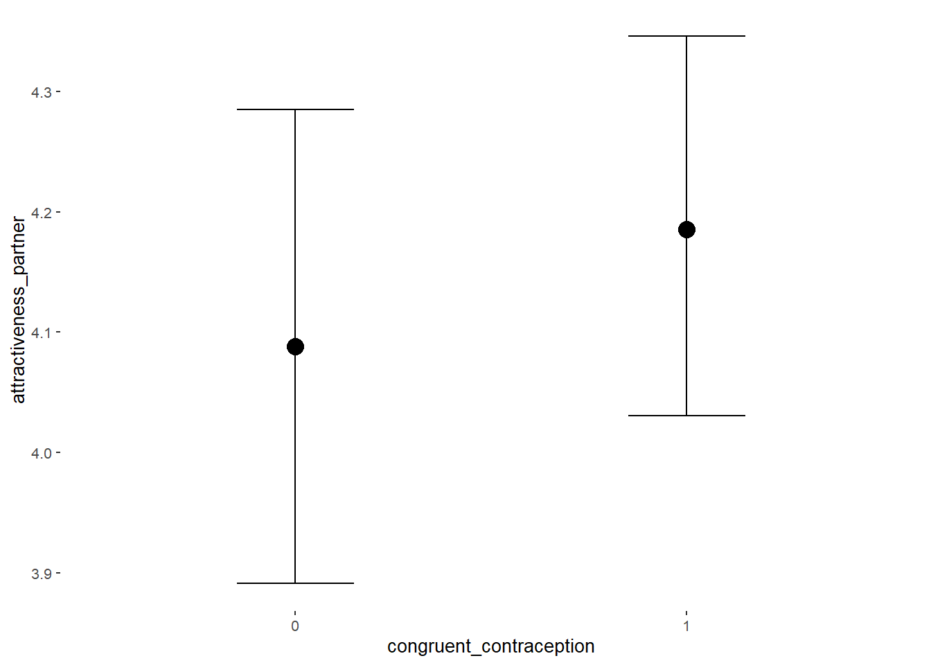
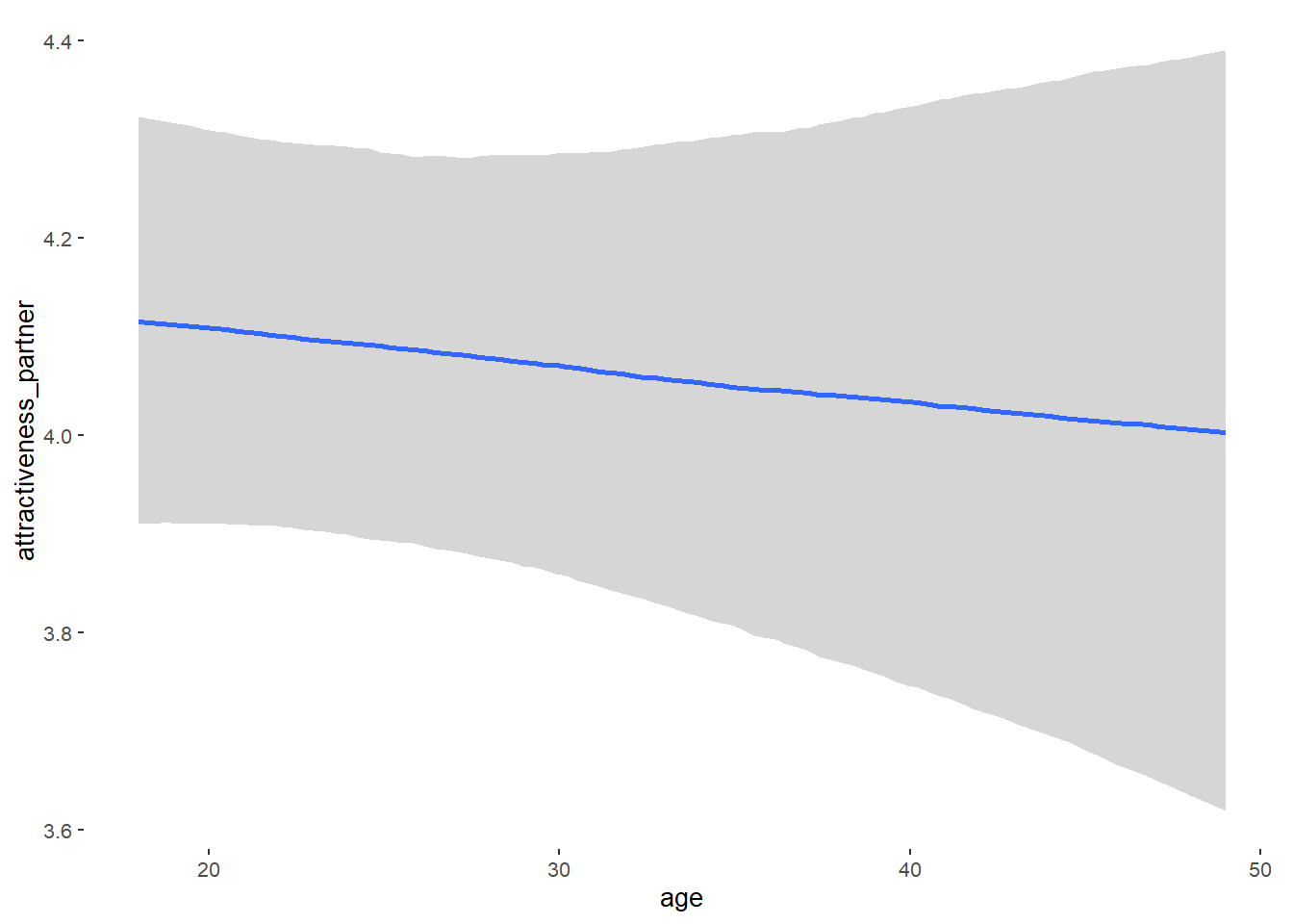
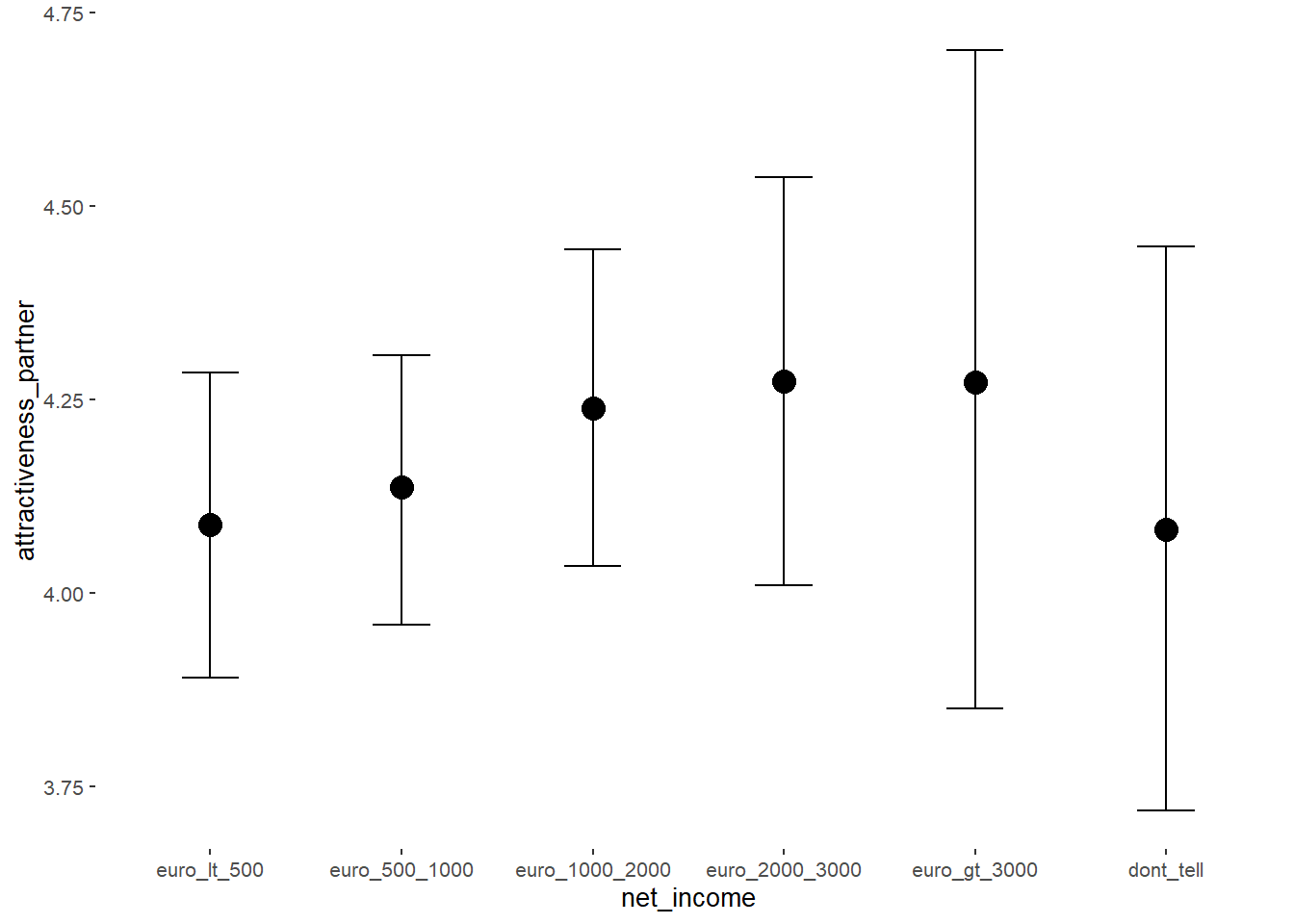
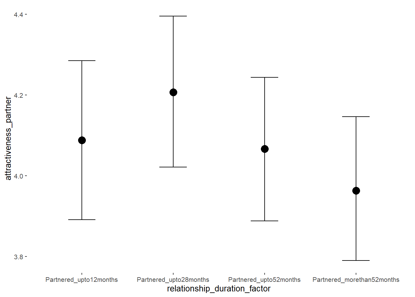
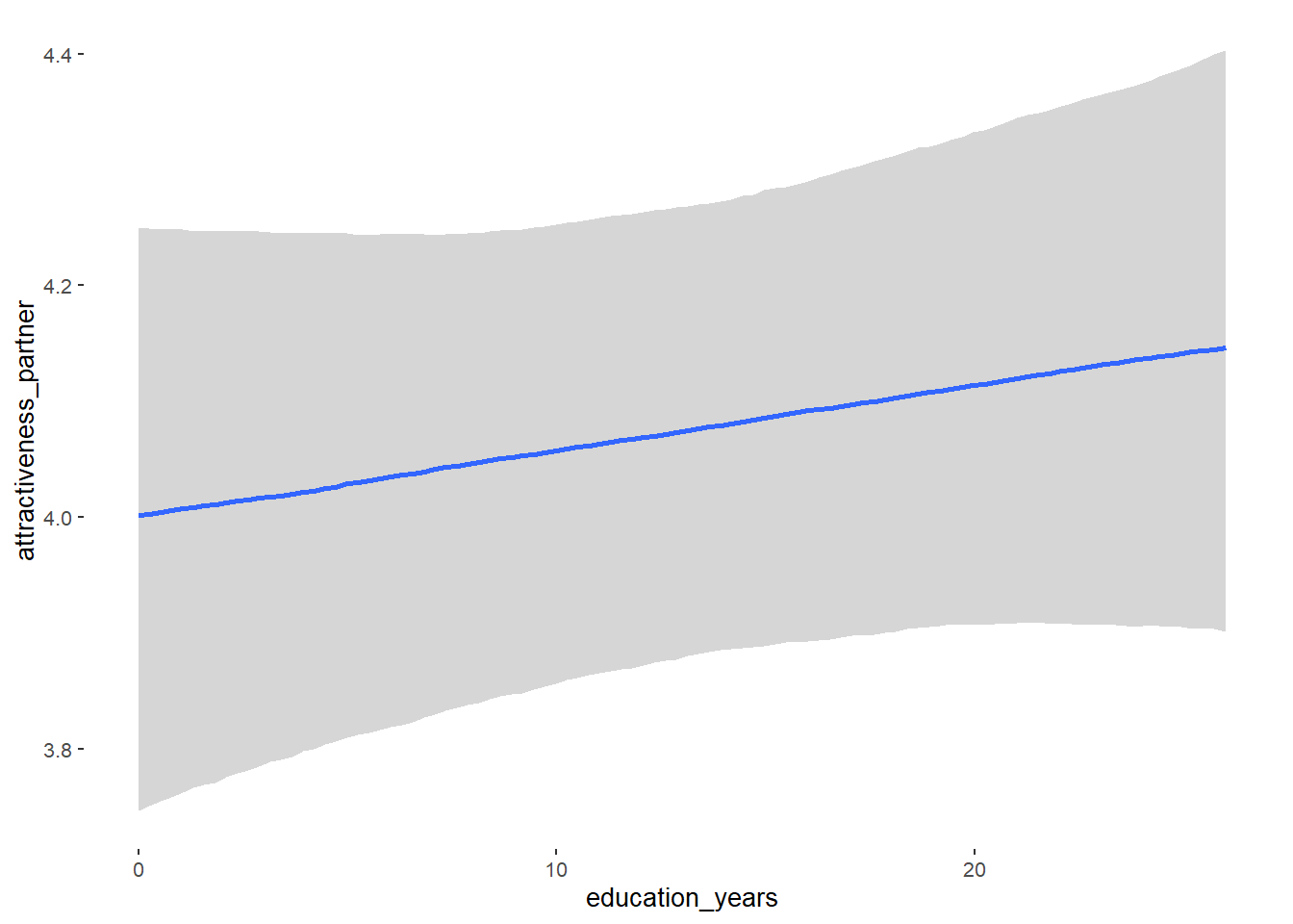
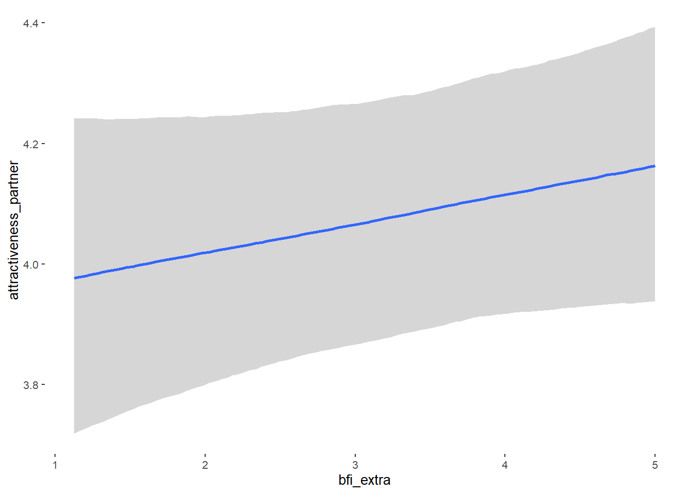
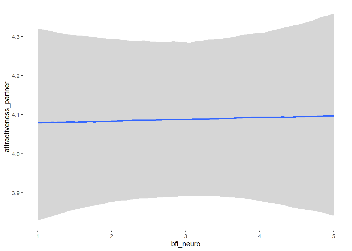
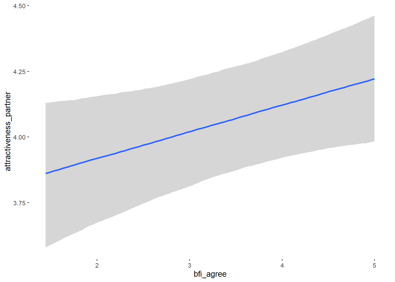
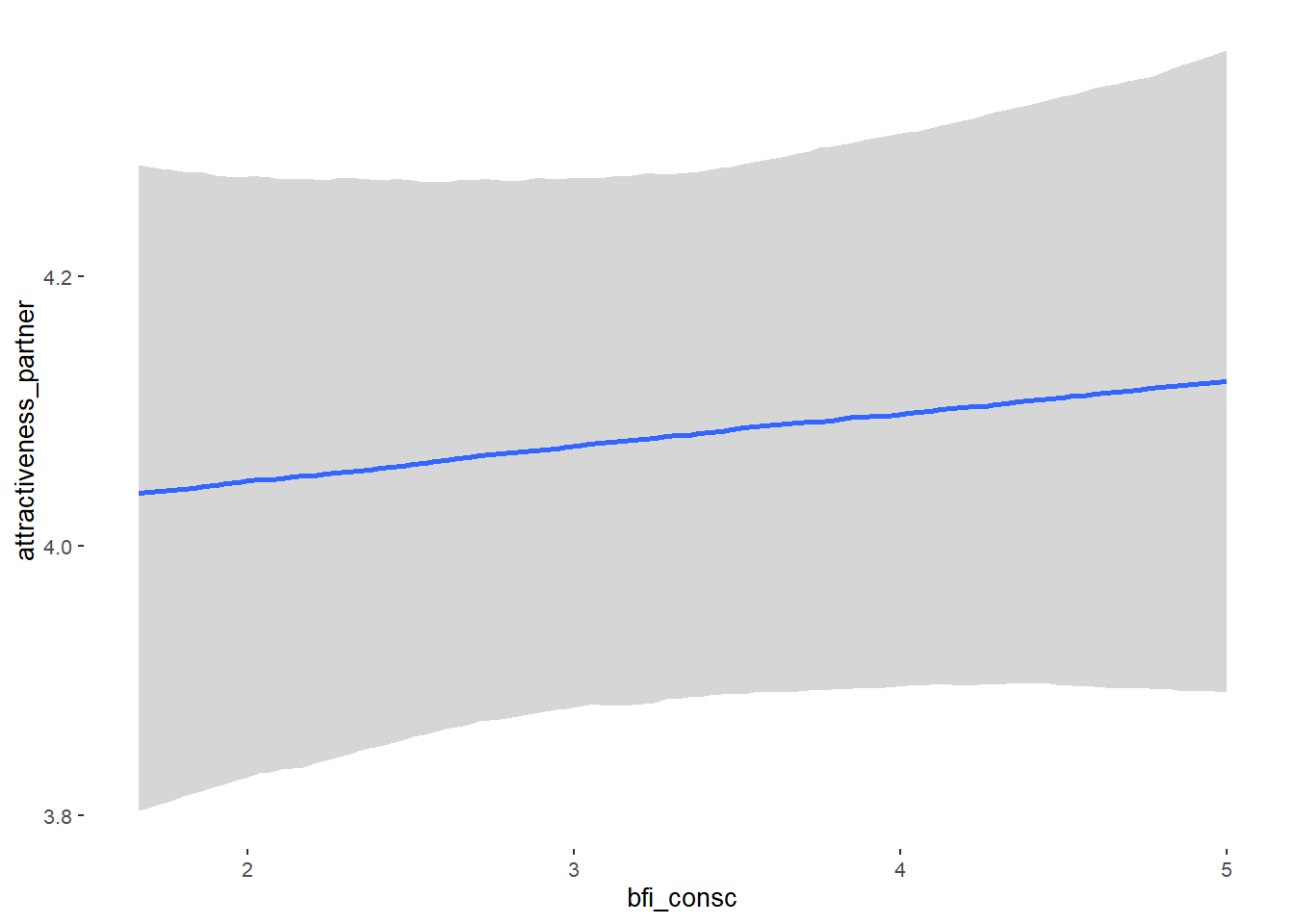
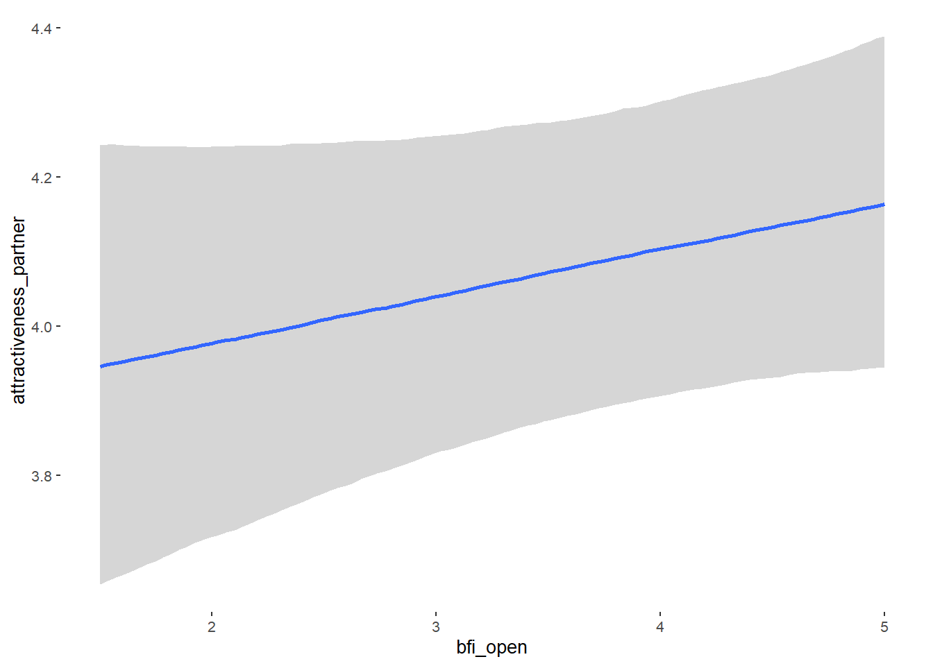
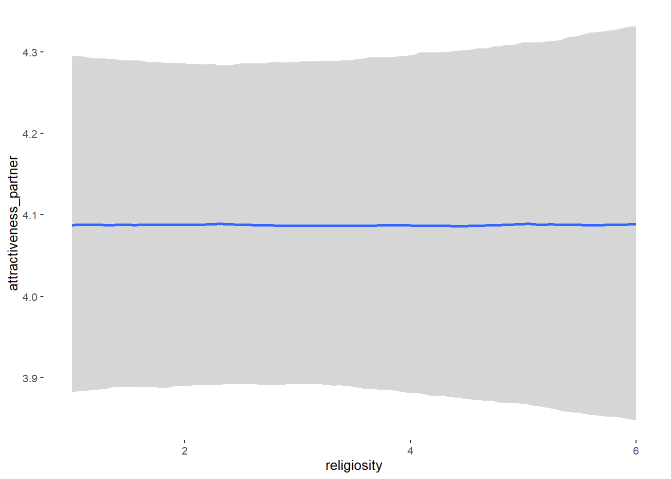
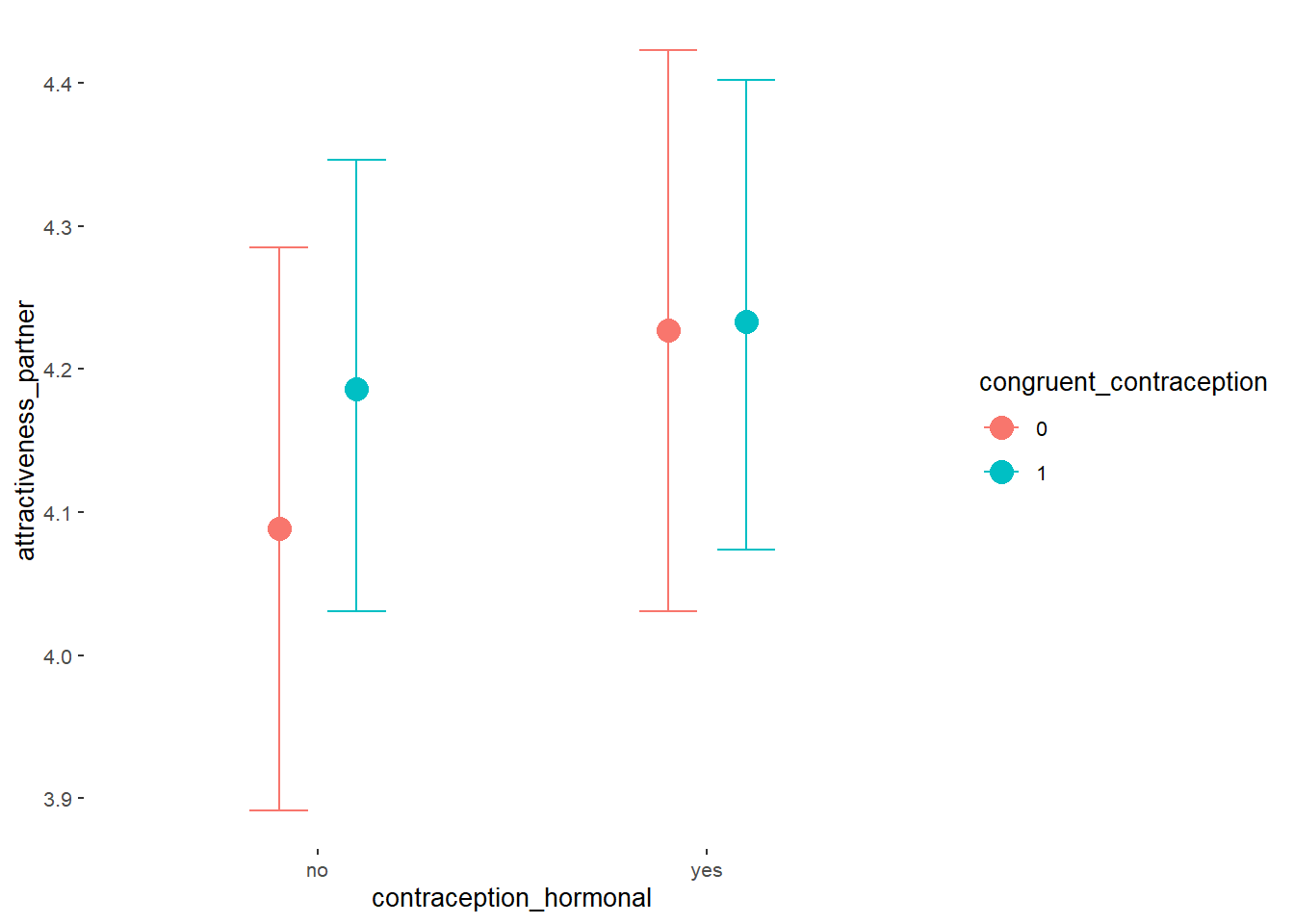
Forest Plot for Effect Sizes
m_congruency_atrr_controlled %>%
  spread_draws(b_contraception_hormonalyes, b_congruent_contraception1,
               `b_contraception_hormonalyes:congruent_contraception1`,
               b_age,
               b_net_incomeeuro_500_1000, b_net_incomeeuro_1000_2000,
               b_net_incomeeuro_2000_3000, b_net_incomeeuro_gt_3000, b_net_incomedont_tell,
               b_relationship_duration_factorPartnered_upto28months,
               b_relationship_duration_factorPartnered_upto52months,
               b_relationship_duration_factorPartnered_morethan52months,
               b_education_years,
               b_bfi_extra, b_bfi_neuro, b_bfi_agree, b_bfi_consc, b_bfi_open,
               b_religiosity) %>%
  pivot_longer(cols = c(b_contraception_hormonalyes, b_congruent_contraception1,
               `b_contraception_hormonalyes:congruent_contraception1`,
                        b_age,
               b_net_incomeeuro_500_1000, b_net_incomeeuro_1000_2000,
               b_net_incomeeuro_2000_3000, b_net_incomeeuro_gt_3000, b_net_incomedont_tell,
               b_relationship_duration_factorPartnered_upto28months,
               b_relationship_duration_factorPartnered_upto52months,
               b_relationship_duration_factorPartnered_morethan52months,
               b_education_years,
               b_bfi_extra, b_bfi_neuro, b_bfi_agree, b_bfi_consc, b_bfi_open,
               b_religiosity),
               names_to = "condition",
               values_to = "r_condition") %>%
  mutate(condition_mean = r_condition,
         group = ifelse(condition %contains% "b_relationship_duration_factor",
                        "Relationship Duration",
                        ifelse(condition %contains% "b_net_income",
                               "Income",
                               NA)),
         group = ifelse(condition %contains% "ontraception",
                        "Contraception", group),
         condition = ifelse(condition == "b_contraception_hormonalyes",
                        "Hormonal Contraception",
                     ifelse(condition == "b_congruent_contraception1",
                            "Congruent Contraception",
                     ifelse(condition == "b_contraception_hormonalyes:congruent_contraception1",
                            "Interaction Hormonal Contracpetion and Congruent Contraception",
                            condition))),
         condition = ifelse(condition == "b_age", "Age",
                ifelse(condition == "b_net_incomeeuro_500_1000", "500-1000 Euro",
                ifelse(condition == "b_net_incomeeuro_1000_2000", "1000-2000 Euro",
                ifelse(condition == "b_net_incomeeuro_2000_3000", "2000-3000 Euro",
                ifelse(condition == "b_net_incomeeuro_gt_3000", ">3000 Euro",
                ifelse(condition == "b_net_incomedont_tell", "do not tell",
                ifelse(condition == "b_relationship_duration_factorPartnered_upto28months",
                       "13-28 months",
                ifelse(condition == "b_relationship_duration_factorPartnered_upto52months",
                       "29-52 months",
                ifelse(condition == "b_relationship_duration_factorPartnered_morethan52months",
                       ">52 months",
                ifelse(condition == "b_education_years", "Years of Education",
                ifelse(condition == "b_bfi_extra", "Extraversion",
                ifelse(condition == "b_bfi_neuro", "Neuroticism",
                ifelse(condition == "b_bfi_agree", "Agreeableness",
                ifelse(condition == "b_bfi_consc", "Conscientiousness",
                ifelse(condition == "b_bfi_open", "Openness",
                ifelse(condition == "b_religiosity", "Religiosity",
                       condition)))))))))))))))),
         group = ifelse(is.na(group), condition, group),
         condition = factor(condition, levels = rev(c("Hormonal Contraception",
                                        "Congruent Contraception",
                                        "Interaction Hormonal Contracpetion and Congruent Contraception",
                                        "Age",
                                        "500-1000 Euro", "1000-2000 Euro",
                                        "2000-3000 Euro", ">3000 Euro", "do not tell",
                                        "13-28 months", "29-52 months",
                                        ">52 months",
                                        "Years of Education",
                                        "Extraversion", "Neuroticism", "Agreeableness",
                                         "Conscientiousness","Openness","Religiosity"))),
         group = factor(group, levels = c("Contraception", "Age", "Income",
                                          "Relationship Duration","Years of Education",
                                          "Extraversion", "Neuroticism", "Agreeableness",
                                         "Conscientiousness","Openness","Religiosity"))) %>%
  ggplot(aes(y = condition,
             x = condition_mean,
             fill = stat(abs(x) < 0.07))) +
  stat_halfeye() +
  geom_vline(xintercept = c(-0.07, 0.07), linetype = "dotted") +
  apatheme +
  theme(legend.position = "none") +
  scale_fill_manual(values = c("gray80", "skyblue")) +
  labs(x = "Effect Size Estimates", y = "Predictors")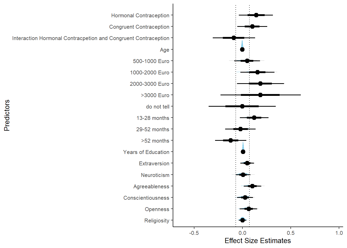
Relationship Satisfaction
Model
m_congruency_relsat_controlled = brm(relationship_satisfaction ~
                          contraception_hormonal * congruent_contraception +
                             age + net_income + relationship_duration_factor +
                              education_years +
                              bfi_extra + bfi_neuro + bfi_agree + bfi_consc + bfi_open +
                              religiosity,
                data = data, family = gaussian(),
                file = "m_congruency_relsat_controlled")
Summary
##  Family: gaussian
##   Links: mu = identity; sigma = identity
## Formula: relationship_satisfaction ~ contraception_hormonal * congruent_contraception + age + net_income + relationship_duration_factor + education_years + bfi_extra + bfi_neuro + bfi_agree + bfi_consc + bfi_open + religiosity
##    Data: data (Number of observations: 774)
##   Draws: 4 chains, each with iter = 2000; warmup = 1000; thin = 1;
##          total post-warmup draws = 4000
##
## Population-Level Effects:
##                                                        Estimate Est.Error l-90% CI u-90% CI Rhat Bulk_ESS
## Intercept                                                  3.31      0.22     2.96     3.68 1.00     5170
## contraception_hormonalyes                                  0.04      0.05    -0.05     0.12 1.00     3344
## congruent_contraception1                                  -0.07      0.04    -0.14     0.01 1.00     3427
## age                                                       -0.00      0.00    -0.01     0.00 1.00     4658
## net_incomeeuro_500_1000                                    0.07      0.04     0.00     0.13 1.00     3823
## net_incomeeuro_1000_2000                                  -0.01      0.05    -0.09     0.07 1.00     3900
## net_incomeeuro_2000_3000                                   0.03      0.07    -0.09     0.14 1.00     3449
## net_incomeeuro_gt_3000                                     0.11      0.12    -0.08     0.30 1.00     4589
## net_incomedont_tell                                       -0.10      0.10    -0.27     0.07 1.00     4754
## relationship_duration_factorPartnered_upto28months         0.20      0.04     0.13     0.27 1.00     3757
## relationship_duration_factorPartnered_upto52months         0.15      0.05     0.08     0.22 1.00     3520
## relationship_duration_factorPartnered_morethan52months     0.13      0.05     0.05     0.20 1.00     3825
## education_years                                           -0.00      0.00    -0.01     0.00 1.00     5870
## bfi_extra                                                  0.02      0.02    -0.01     0.05 1.00     4186
## bfi_neuro                                                  0.03      0.02    -0.01     0.07 1.00     4381
## bfi_agree                                                 -0.02      0.03    -0.07     0.02 1.00     4860
## bfi_consc                                                  0.01      0.02    -0.04     0.05 1.00     5180
## bfi_open                                                  -0.01      0.03    -0.06     0.03 1.00     5037
## religiosity                                                0.03      0.01     0.01     0.05 1.00     4740
## contraception_hormonalyes:congruent_contraception1         0.03      0.06    -0.07     0.14 1.00     2955
##                                                        Tail_ESS
## Intercept                                                  3333
## contraception_hormonalyes                                  2833
## congruent_contraception1                                   2906
## age                                                        3556
## net_incomeeuro_500_1000                                    3101
## net_incomeeuro_1000_2000                                   3363
## net_incomeeuro_2000_3000                                   3233
## net_incomeeuro_gt_3000                                     3302
## net_incomedont_tell                                        3396
## relationship_duration_factorPartnered_upto28months         2670
## relationship_duration_factorPartnered_upto52months         3015
## relationship_duration_factorPartnered_morethan52months     3290
## education_years                                            3045
## bfi_extra                                                  2997
## bfi_neuro                                                  3294
## bfi_agree                                                  3249
## bfi_consc                                                  3217
## bfi_open                                                   3099
## religiosity                                                2961
## contraception_hormonalyes:congruent_contraception1         2483
##
## Family Specific Parameters:
##       Estimate Est.Error l-90% CI u-90% CI Rhat Bulk_ESS Tail_ESS
## sigma     0.41      0.01     0.40     0.43 1.00     4750     3091
##
## Draws were sampled using sampling(NUTS). For each parameter, Bulk_ESS
## and Tail_ESS are effective sample size measures, and Rhat is the potential
## scale reduction factor on split chains (at convergence, Rhat = 1).
Comparison with ROPE
plot(equivalence_test(m_congruency_relsat_controlled, range = c(-0.04, 0.04), ci = 0.90,
                      parameters = "contraception"))
## Possible multicollinearity between b_contraception_hormonalyes:congruent_contraception1 and b_contraception_hormonalyes (r = 0.77). This might lead to inappropriate results. See 'Details' in '?equivalence_test'.## Picking joint bandwidth of 0.0073## Warning: Removed 1197 rows containing non-finite values (stat_density_ridges).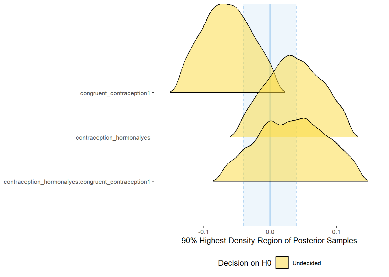
equivalence_test(m_congruency_relsat_controlled, range = c(-0.04, 0.04), ci = 0.90,
                      parameters = "contraception")
## Possible multicollinearity between b_contraception_hormonalyes:congruent_contraception1 and b_contraception_hormonalyes (r = 0.77). This might lead to inappropriate results. See 'Details' in '?equivalence_test'.## # A tibble: 3 x 10
## Parameter CI ROPE_low ROPE_high ROPE_Percentage ROPE_Equivalence HDI_low HDI_high Effects Component
## <chr> <dbl> <dbl> <dbl> <dbl> <chr> <dbl> <dbl> <chr> <chr>
## 1 b_contraceptio~ 0.9 -0.04 0.04 0.520 Undecided -0.0470 0.119 fixed conditio~
## 2 b_congruent_co~ 0.9 -0.04 0.04 0.260 Undecided -0.137 0.00916 fixed conditio~
## 3 b_contraceptio~ 0.9 -0.04 0.04 0.459 Undecided -0.0731 0.136 fixed conditio~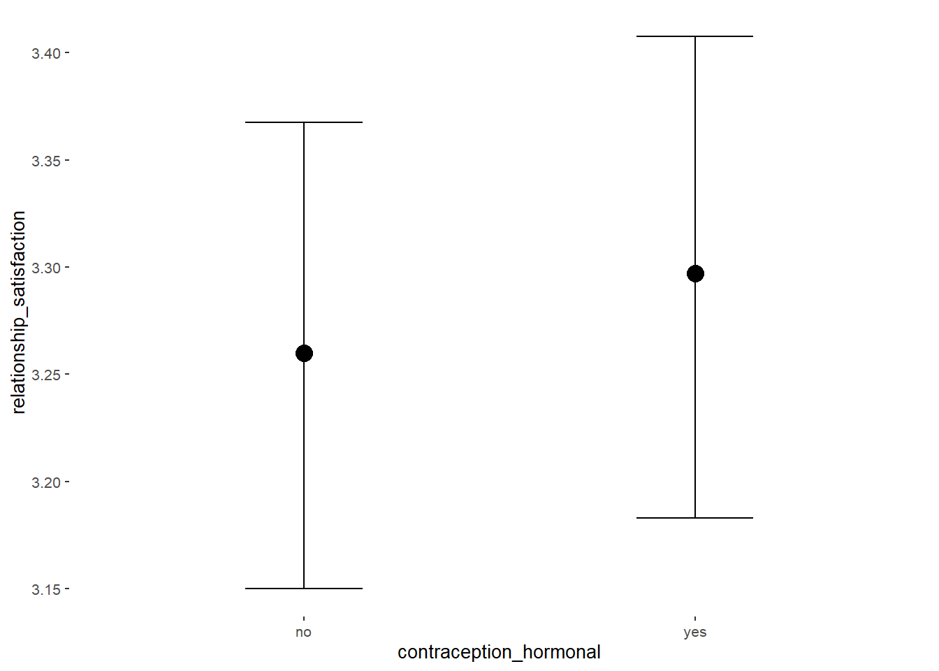
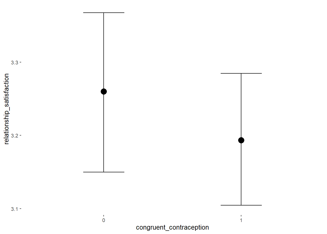
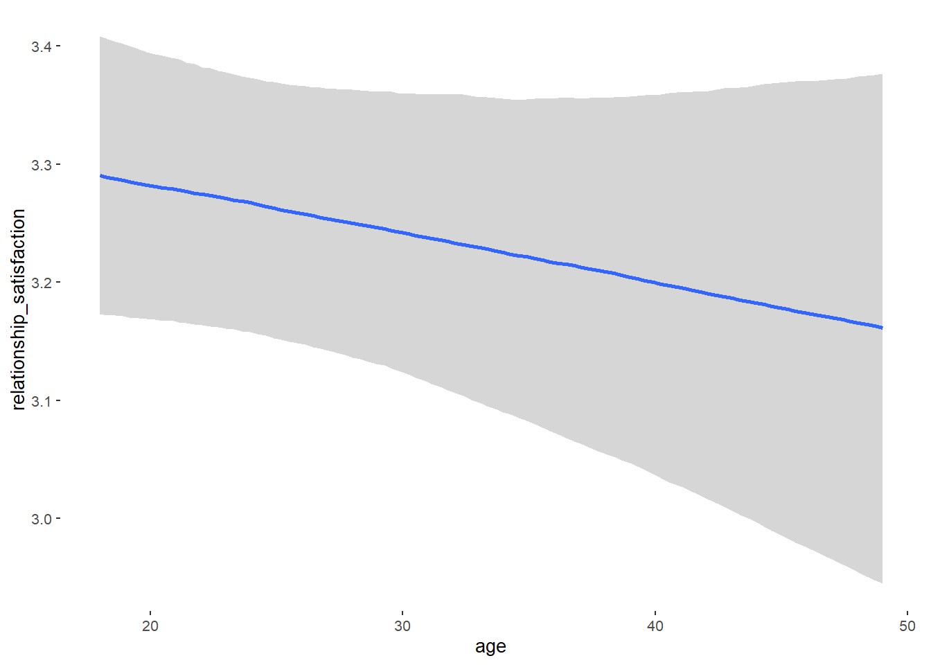
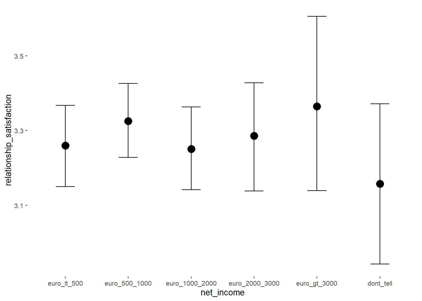
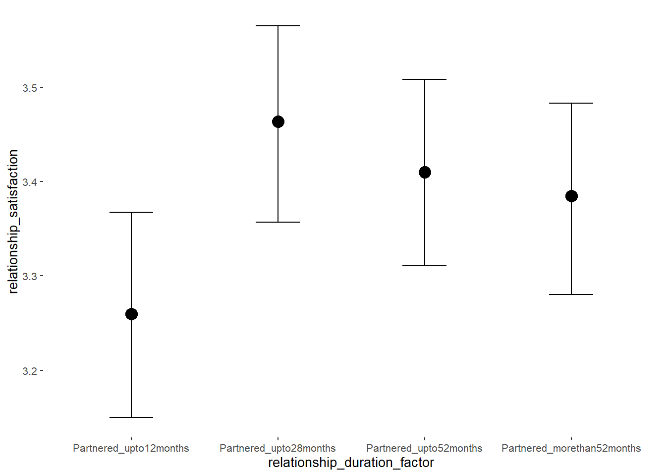
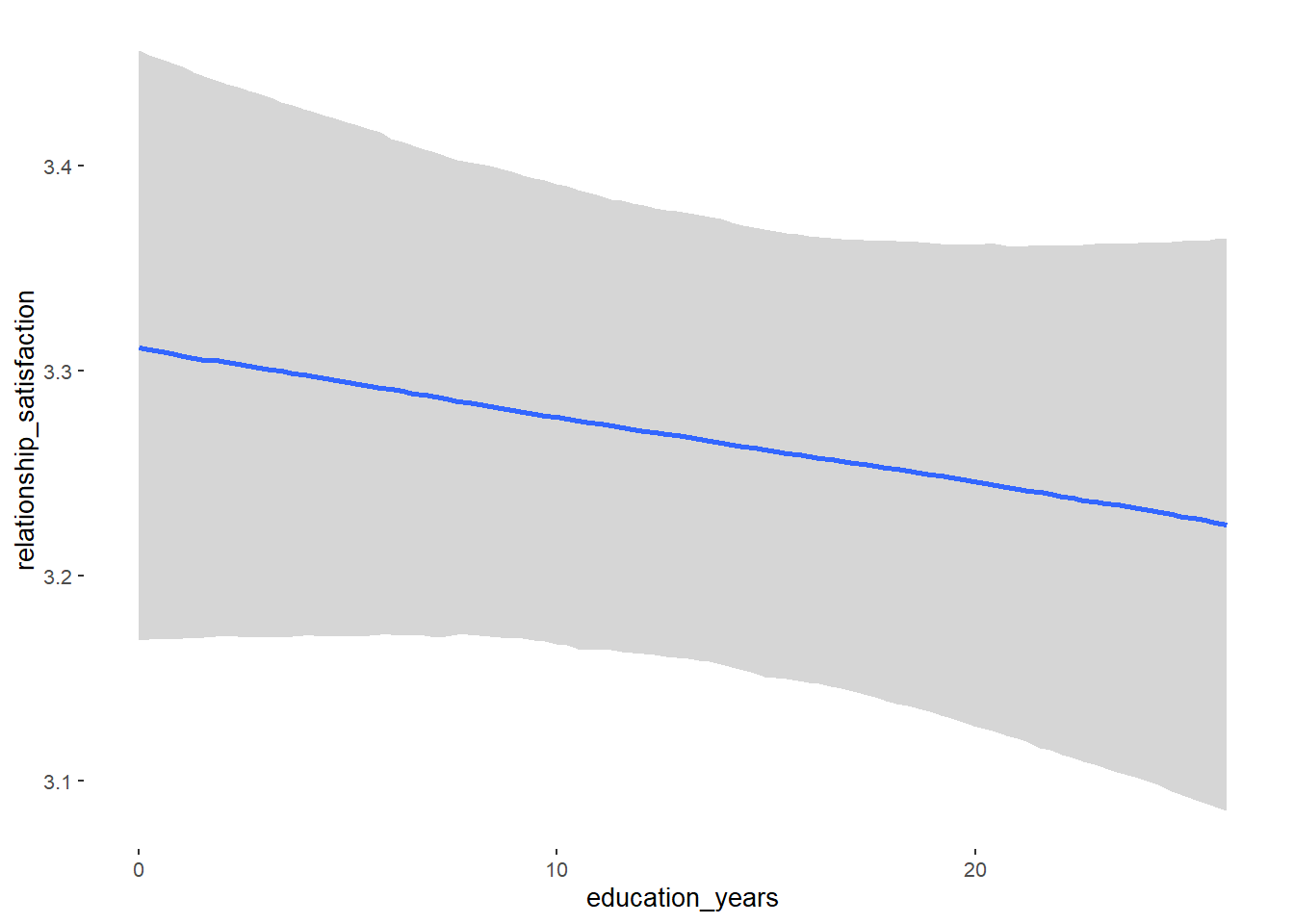
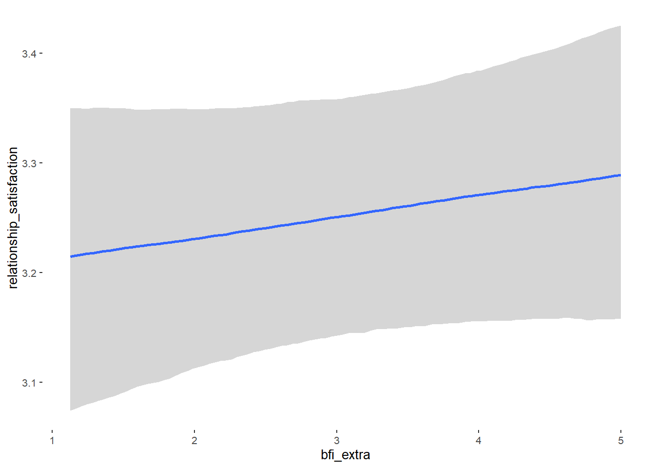
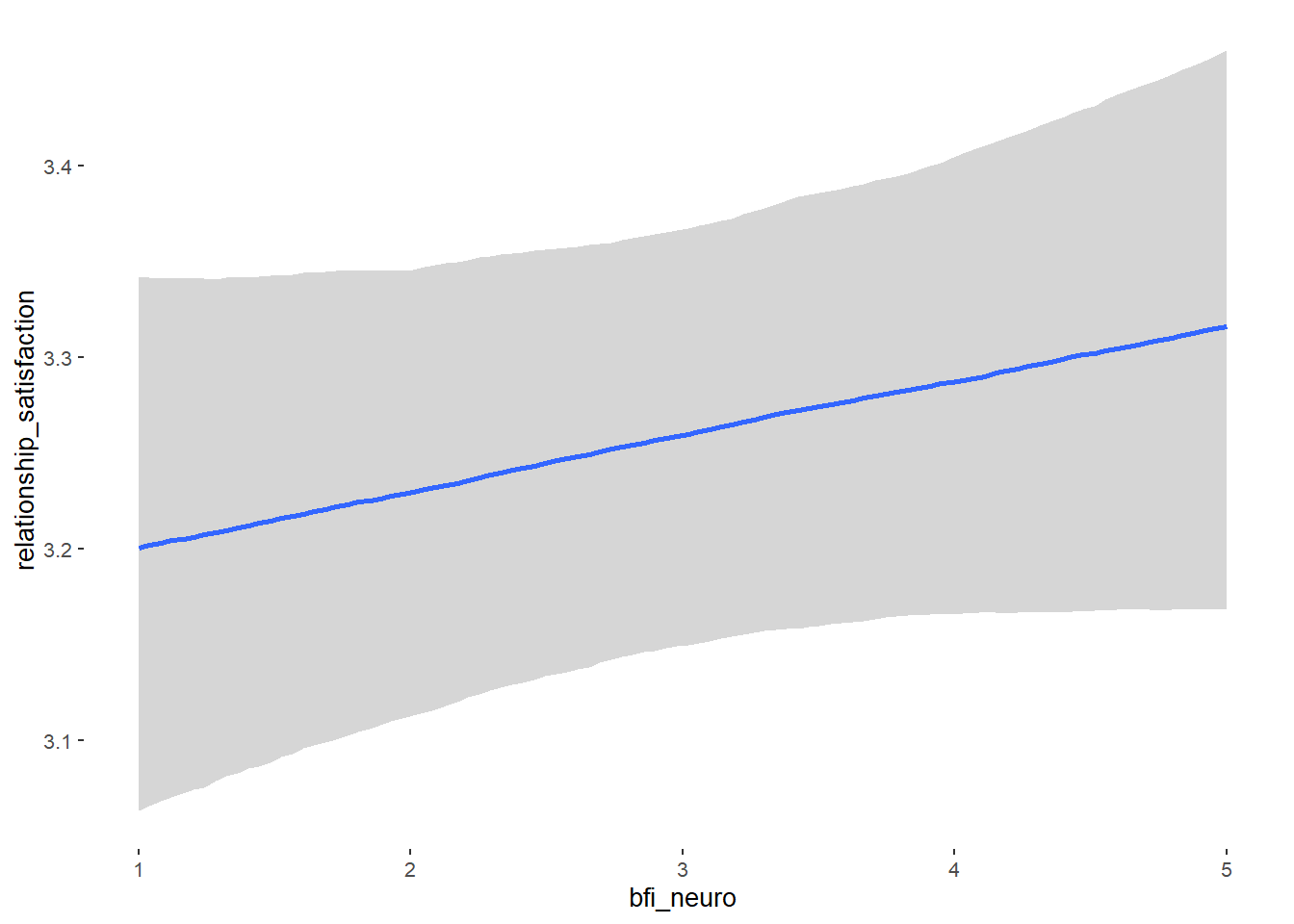
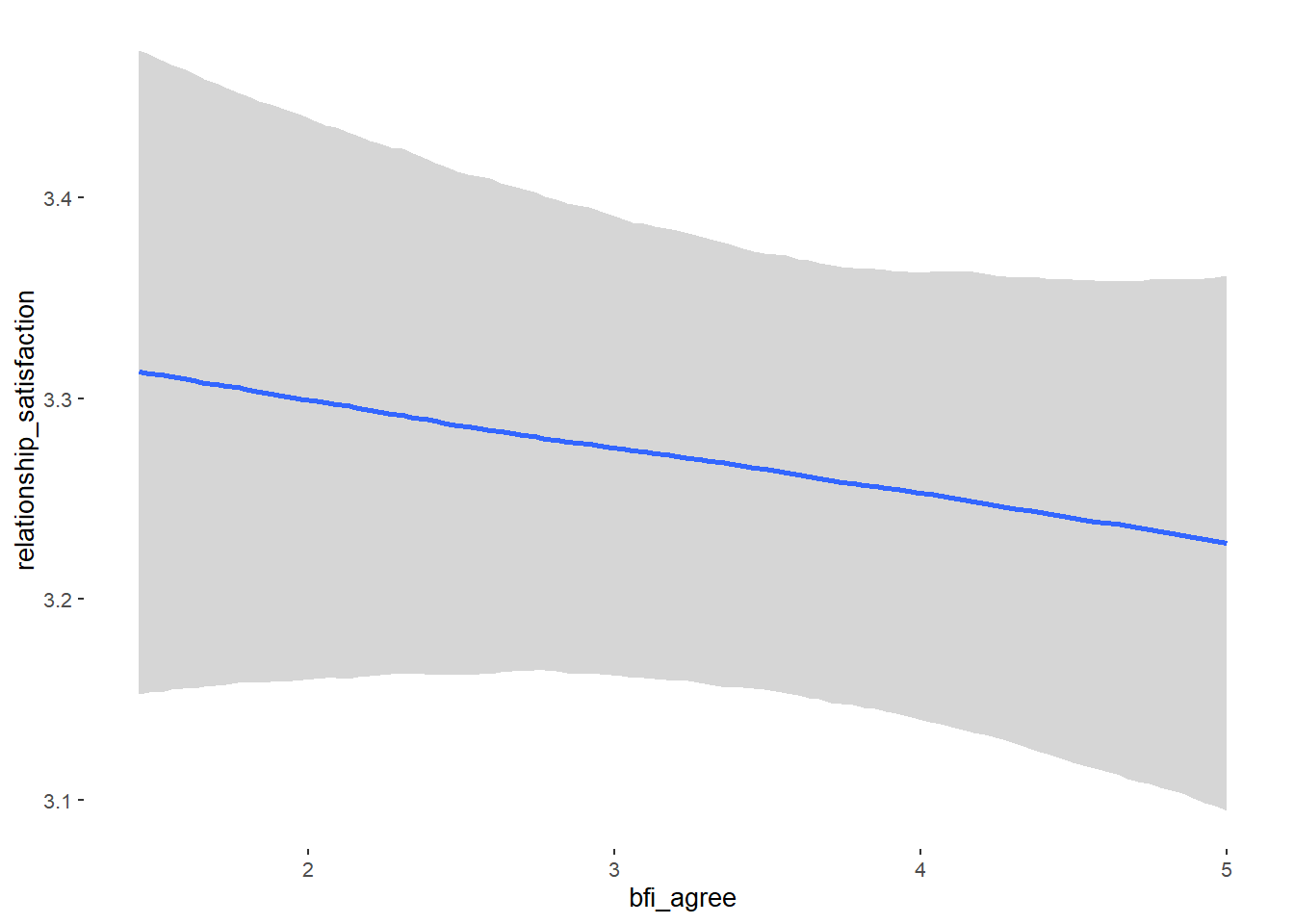
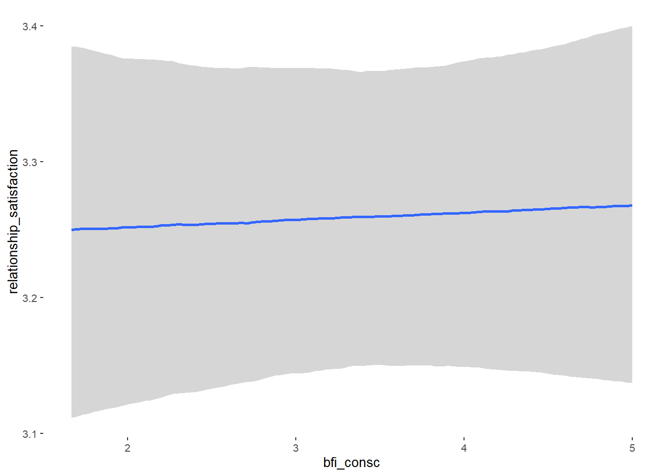
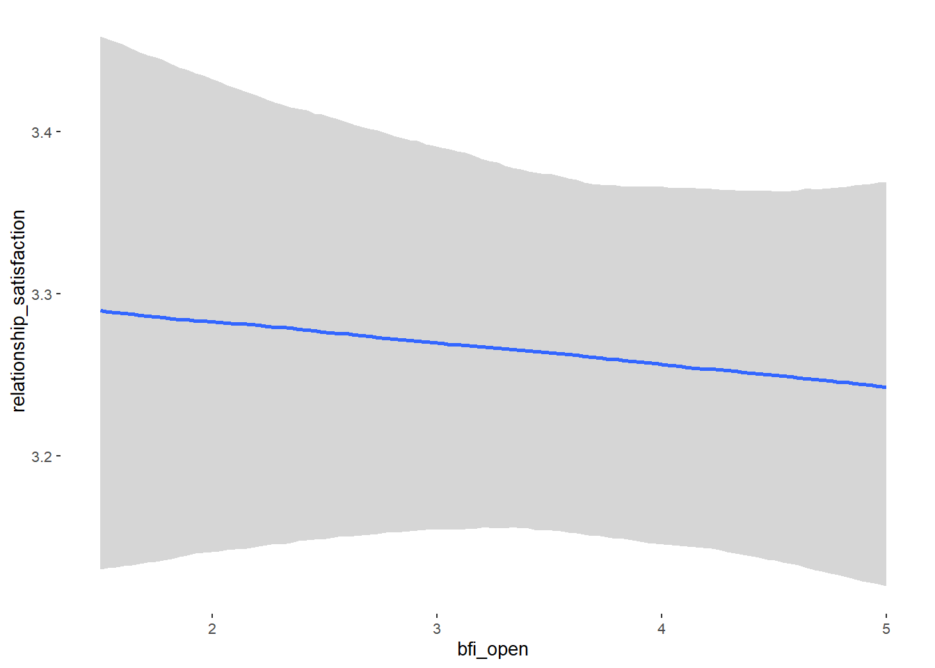
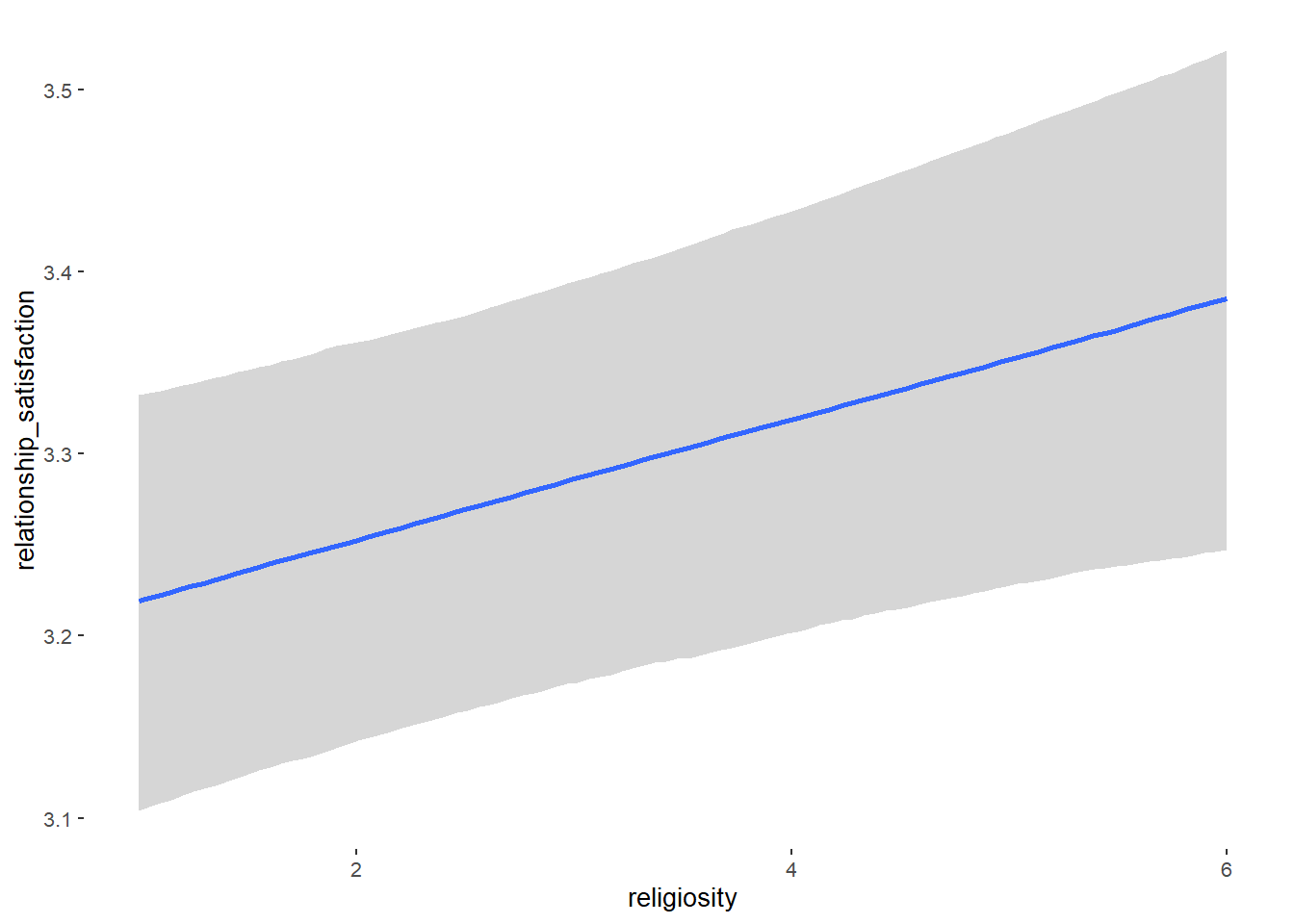
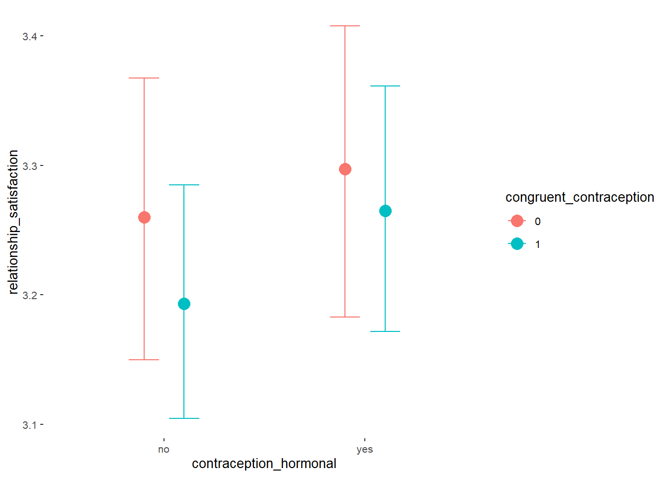
Forest Plot for Effect Sizes
m_congruency_relsat_controlled %>%

  spread_draws(b_contraception_hormonalyes, b_congruent_contraception1,
               `b_contraception_hormonalyes:congruent_contraception1`,
               b_age,
               b_net_incomeeuro_500_1000, b_net_incomeeuro_1000_2000,
               b_net_incomeeuro_2000_3000, b_net_incomeeuro_gt_3000, b_net_incomedont_tell,
               b_relationship_duration_factorPartnered_upto28months,
               b_relationship_duration_factorPartnered_upto52months,
               b_relationship_duration_factorPartnered_morethan52months,
               b_education_years,
               b_bfi_extra, b_bfi_neuro, b_bfi_agree, b_bfi_consc, b_bfi_open,
               b_religiosity) %>%
  pivot_longer(cols = c(b_contraception_hormonalyes, b_congruent_contraception1,
               `b_contraception_hormonalyes:congruent_contraception1`,
                        b_age,
               b_net_incomeeuro_500_1000, b_net_incomeeuro_1000_2000,
               b_net_incomeeuro_2000_3000, b_net_incomeeuro_gt_3000, b_net_incomedont_tell,
               b_relationship_duration_factorPartnered_upto28months,
               b_relationship_duration_factorPartnered_upto52months,
               b_relationship_duration_factorPartnered_morethan52months,
               b_education_years,
               b_bfi_extra, b_bfi_neuro, b_bfi_agree, b_bfi_consc, b_bfi_open,
               b_religiosity),
               names_to = "condition",
               values_to = "r_condition") %>%
  mutate(condition_mean = r_condition,
         group = ifelse(condition %contains% "b_relationship_duration_factor",
                        "Relationship Duration",
                        ifelse(condition %contains% "b_net_income",
                               "Income",
                               NA)),
         group = ifelse(condition %contains% "ontraception",
                        "Contraception", group),
         condition = ifelse(condition == "b_contraception_hormonalyes",
                        "Hormonal Contraception",
                     ifelse(condition == "b_congruent_contraception1",
                            "Congruent Contraception",
                     ifelse(condition == "b_contraception_hormonalyes:congruent_contraception1",
                            "Interaction Hormonal Contracpetion and Congruent Contraception",
                            condition))),
         condition = ifelse(condition == "b_age", "Age",
                ifelse(condition == "b_net_incomeeuro_500_1000", "500-1000 Euro",
                ifelse(condition == "b_net_incomeeuro_1000_2000", "1000-2000 Euro",
                ifelse(condition == "b_net_incomeeuro_2000_3000", "2000-3000 Euro",
                ifelse(condition == "b_net_incomeeuro_gt_3000", ">3000 Euro",
                ifelse(condition == "b_net_incomedont_tell", "do not tell",
                ifelse(condition == "b_relationship_duration_factorPartnered_upto28months",
                       "13-28 months",
                ifelse(condition == "b_relationship_duration_factorPartnered_upto52months",
                       "29-52 months",
                ifelse(condition == "b_relationship_duration_factorPartnered_morethan52months",
                       ">52 months",
                ifelse(condition == "b_education_years", "Years of Education",
                ifelse(condition == "b_bfi_extra", "Extraversion",
                ifelse(condition == "b_bfi_neuro", "Neuroticism",
                ifelse(condition == "b_bfi_agree", "Agreeableness",
                ifelse(condition == "b_bfi_consc", "Conscientiousness",
                ifelse(condition == "b_bfi_open", "Openness",
                ifelse(condition == "b_religiosity", "Religiosity",
                       condition)))))))))))))))),
         group = ifelse(is.na(group), condition, group),
         condition = factor(condition, levels = rev(c("Hormonal Contraception",
                                        "Congruent Contraception",
                                        "Interaction Hormonal Contracpetion and Congruent Contraception",
                                        "Age",
                                        "500-1000 Euro", "1000-2000 Euro",
                                        "2000-3000 Euro", ">3000 Euro", "do not tell",
                                        "13-28 months", "29-52 months",
                                        ">52 months",
                                        "Years of Education",
                                        "Extraversion", "Neuroticism", "Agreeableness",
                                         "Conscientiousness","Openness","Religiosity"))),
         group = factor(group, levels = c("Contraception", "Age", "Income",
                                          "Relationship Duration","Years of Education",
                                          "Extraversion", "Neuroticism", "Agreeableness",
                                         "Conscientiousness","Openness","Religiosity"))) %>%
  ggplot(aes(y = condition,
             x = condition_mean,
             fill = stat(abs(x) < 0.04))) +
  stat_halfeye() +
  geom_vline(xintercept = c(-0.04, 0.04), linetype = "dotted") +
  apatheme +
  theme(legend.position = "none") +
  scale_fill_manual(values = c("gray80", "skyblue")) +
  labs(x = "Effect Size Estimates", y = "Predictors")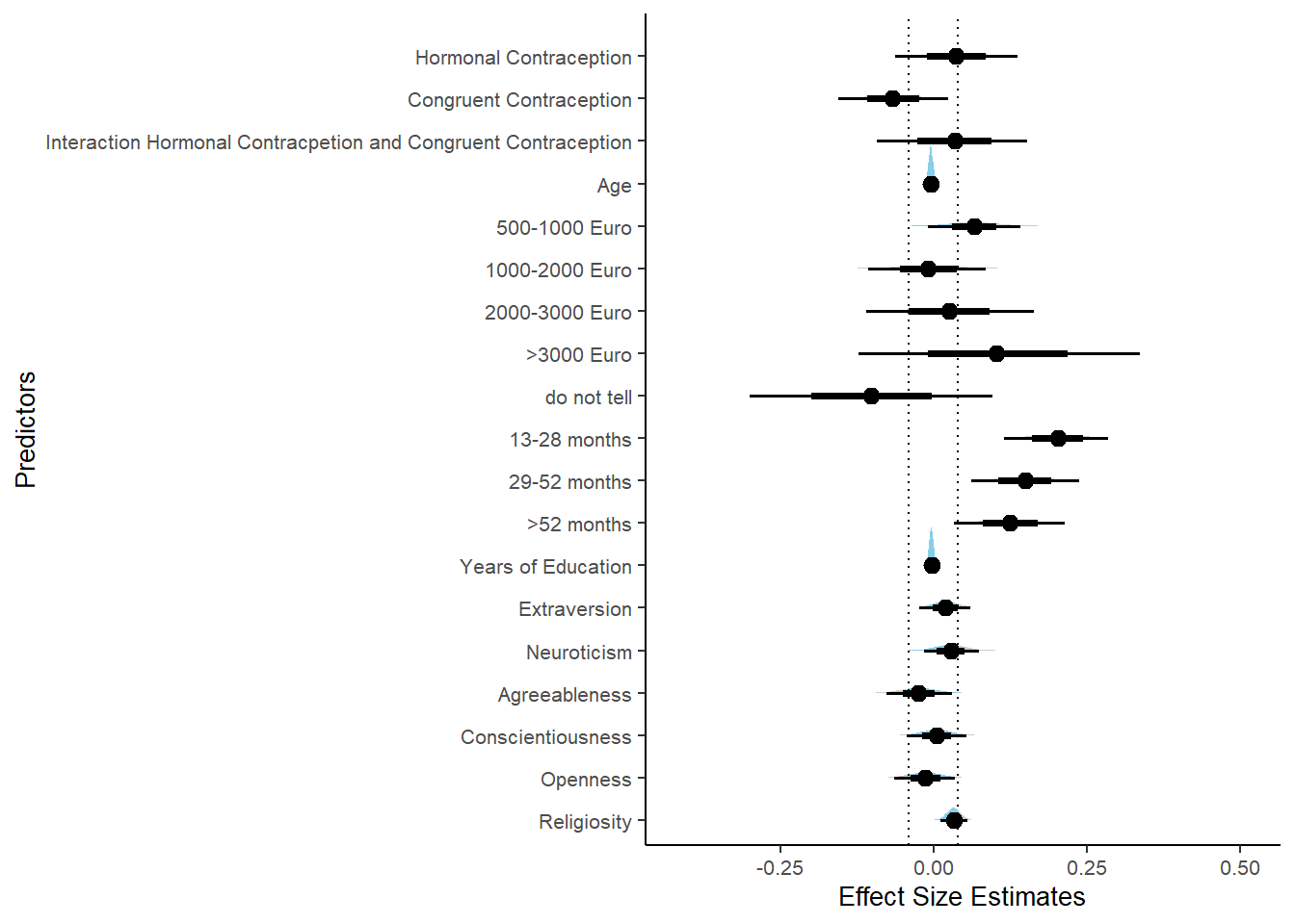
Sexual Satisfaction
Model
m_congruency_sexsat_controlled = brm(satisfaction_sexual_intercourse ~
                          contraception_hormonal * congruent_contraception +
                             age + net_income + relationship_duration_factor +
                              education_years +
                              bfi_extra + bfi_neuro + bfi_agree + bfi_consc + bfi_open +
                              religiosity,
                data = data, family = gaussian(),
                file = "m_congruency_sexsat_controlled")
Summary
##  Family: gaussian
##   Links: mu = identity; sigma = identity
## Formula: satisfaction_sexual_intercourse ~ contraception_hormonal * congruent_contraception + age + net_income + relationship_duration_factor + education_years + bfi_extra + bfi_neuro + bfi_agree + bfi_consc + bfi_open + religiosity
##    Data: data (Number of observations: 774)
##   Draws: 4 chains, each with iter = 2000; warmup = 1000; thin = 1;
##          total post-warmup draws = 4000
##
## Population-Level Effects:
##                                                        Estimate Est.Error l-90% CI u-90% CI Rhat Bulk_ESS
## Intercept                                                  3.18      0.55     2.28     4.07 1.00     4935
## contraception_hormonalyes                                  0.12      0.13    -0.10     0.33 1.00     3289
## congruent_contraception1                                   0.04      0.12    -0.15     0.23 1.00     3444
## age                                                        0.01      0.01    -0.01     0.02 1.00     4130
## net_incomeeuro_500_1000                                    0.03      0.10    -0.13     0.18 1.00     3957
## net_incomeeuro_1000_2000                                  -0.08      0.13    -0.29     0.13 1.00     3414
## net_incomeeuro_2000_3000                                  -0.08      0.18    -0.37     0.21 1.00     4057
## net_incomeeuro_gt_3000                                    -0.26      0.30    -0.75     0.24 1.00     4579
## net_incomedont_tell                                       -0.04      0.25    -0.46     0.36 1.00     4603
## relationship_duration_factorPartnered_upto28months        -0.02      0.11    -0.19     0.16 1.00     4262
## relationship_duration_factorPartnered_upto52months        -0.23      0.11    -0.42    -0.05 1.00     4104
## relationship_duration_factorPartnered_morethan52months    -0.37      0.12    -0.56    -0.18 1.00     4017
## education_years                                           -0.00      0.01    -0.02     0.01 1.00     5468
## bfi_extra                                                  0.11      0.05     0.02     0.19 1.00     5191
## bfi_neuro                                                 -0.07      0.06    -0.17     0.02 1.00     4528
## bfi_agree                                                  0.13      0.07     0.03     0.24 1.00     5064
## bfi_consc                                                  0.14      0.06     0.04     0.23 1.00     5904
## bfi_open                                                  -0.10      0.06    -0.20     0.01 1.00     5260
## religiosity                                               -0.01      0.03    -0.05     0.04 1.00     5701
## contraception_hormonalyes:congruent_contraception1        -0.01      0.17    -0.28     0.26 1.00     3163
##                                                        Tail_ESS
## Intercept                                                  2946
## contraception_hormonalyes                                  2883
## congruent_contraception1                                   3135
## age                                                        2864
## net_incomeeuro_500_1000                                    3187
## net_incomeeuro_1000_2000                                   2932
## net_incomeeuro_2000_3000                                   2994
## net_incomeeuro_gt_3000                                     3080
## net_incomedont_tell                                        2890
## relationship_duration_factorPartnered_upto28months         3210
## relationship_duration_factorPartnered_upto52months         2756
## relationship_duration_factorPartnered_morethan52months     2881
## education_years                                            2948
## bfi_extra                                                  3176
## bfi_neuro                                                  3091
## bfi_agree                                                  2730
## bfi_consc                                                  2967
## bfi_open                                                   3048
## religiosity                                                3140
## contraception_hormonalyes:congruent_contraception1         3035
##
## Family Specific Parameters:
##       Estimate Est.Error l-90% CI u-90% CI Rhat Bulk_ESS Tail_ESS
## sigma     1.03      0.03     0.99     1.08 1.00     4869     3374
##
## Draws were sampled using sampling(NUTS). For each parameter, Bulk_ESS
## and Tail_ESS are effective sample size measures, and Rhat is the potential
## scale reduction factor on split chains (at convergence, Rhat = 1).
Comparison with ROPE
plot(equivalence_test(m_congruency_sexsat_controlled, range = c(-0.11, 0.11), ci = 0.90,
                      parameters = "contraception"))
## Possible multicollinearity between b_contraception_hormonalyes:congruent_contraception1 and b_contraception_hormonalyes (r = 0.78), b_contraception_hormonalyes:congruent_contraception1 and b_congruent_contraception1 (r = 0.72). This might lead to inappropriate results. See 'Details' in '?equivalence_test'.## Picking joint bandwidth of 0.0189## Warning: Removed 1197 rows containing non-finite values (stat_density_ridges).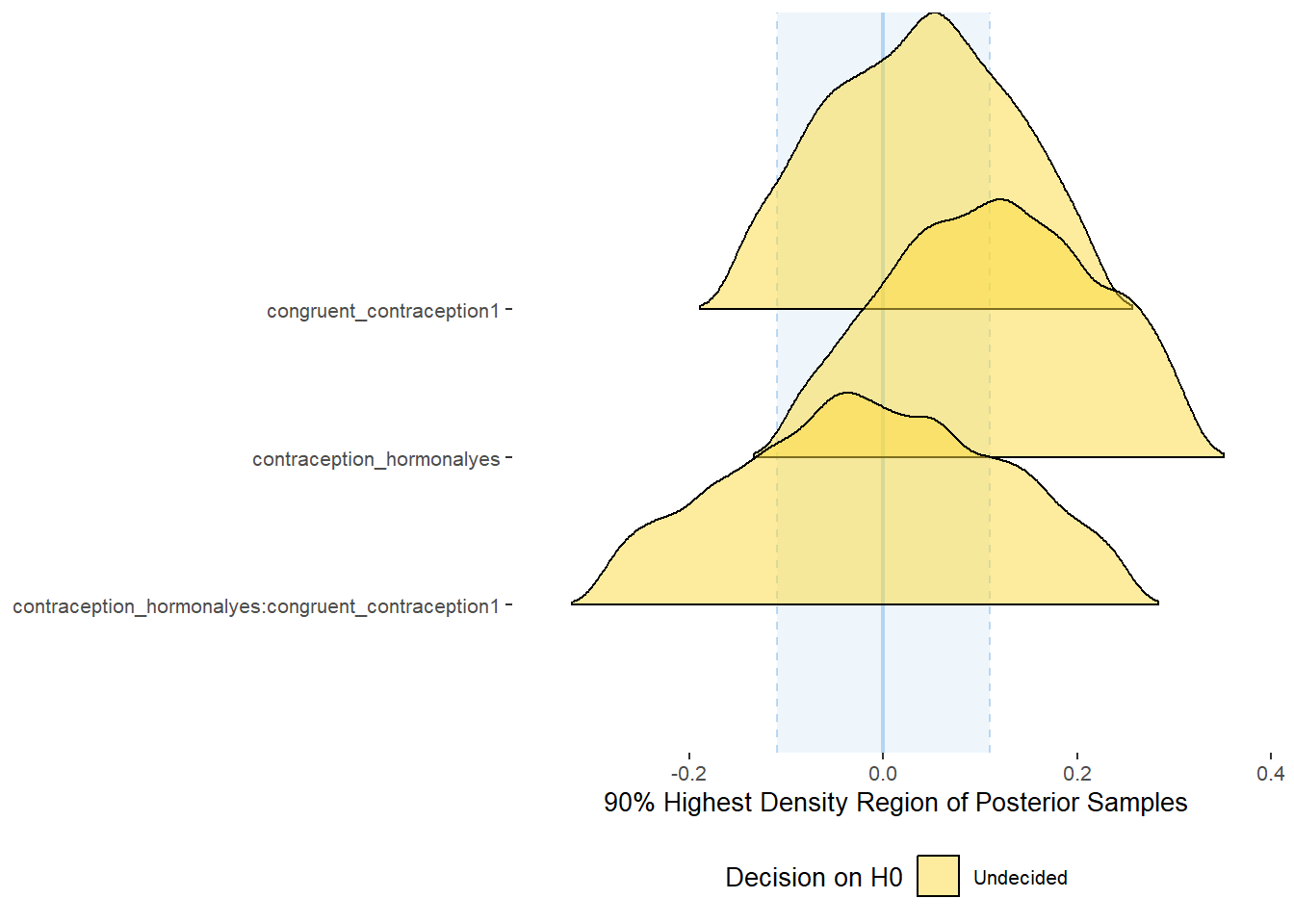
equivalence_test(m_congruency_sexsat_controlled, range = c(-0.11, 0.11), ci = 0.90,
                      parameters = "contraception")
## Possible multicollinearity between b_contraception_hormonalyes:congruent_contraception1 and b_contraception_hormonalyes (r = 0.78), b_contraception_hormonalyes:congruent_contraception1 and b_congruent_contraception1 (r = 0.72). This might lead to inappropriate results. See 'Details' in '?equivalence_test'.## # A tibble: 3 x 10
## Parameter CI ROPE_low ROPE_high ROPE_Percentage ROPE_Equivalence HDI_low HDI_high Effects Component
## <chr> <dbl> <dbl> <dbl> <dbl> <chr> <dbl> <dbl> <chr> <chr>
## 1 b_contraceptio~ 0.9 -0.11 0.11 0.490 Undecided -0.102 0.317 fixed conditio~
## 2 b_congruent_co~ 0.9 -0.11 0.11 0.705 Undecided -0.155 0.222 fixed conditio~
## 3 b_contraceptio~ 0.9 -0.11 0.11 0.547 Undecided -0.290 0.253 fixed conditio~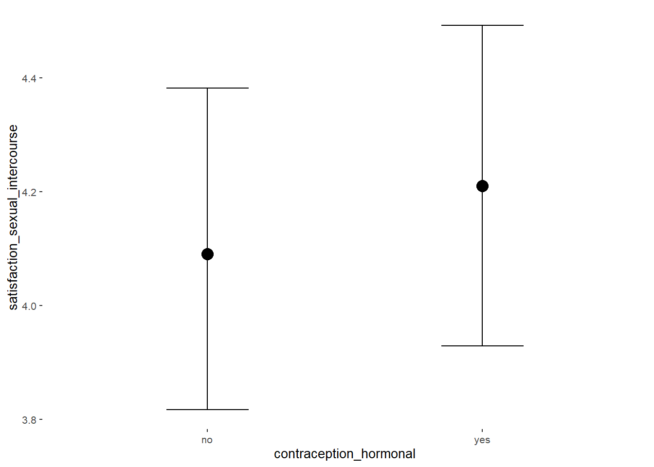
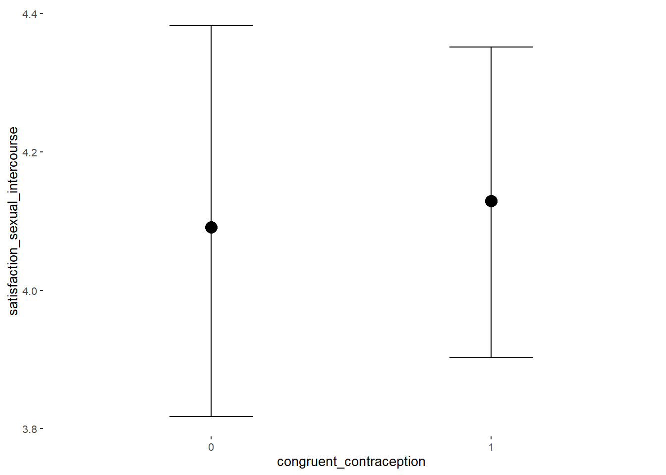
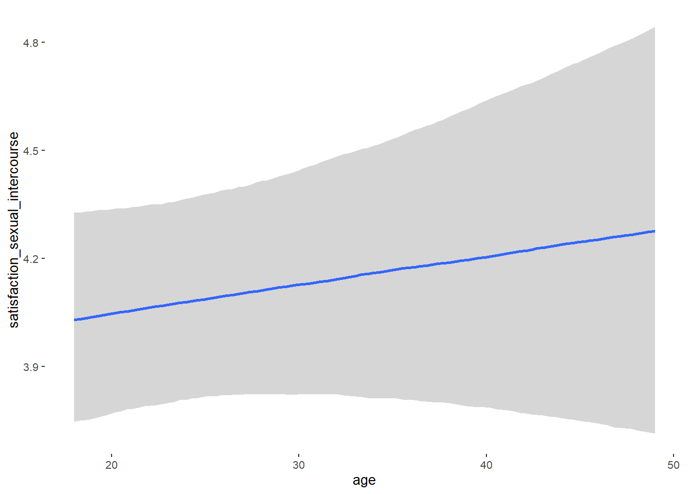
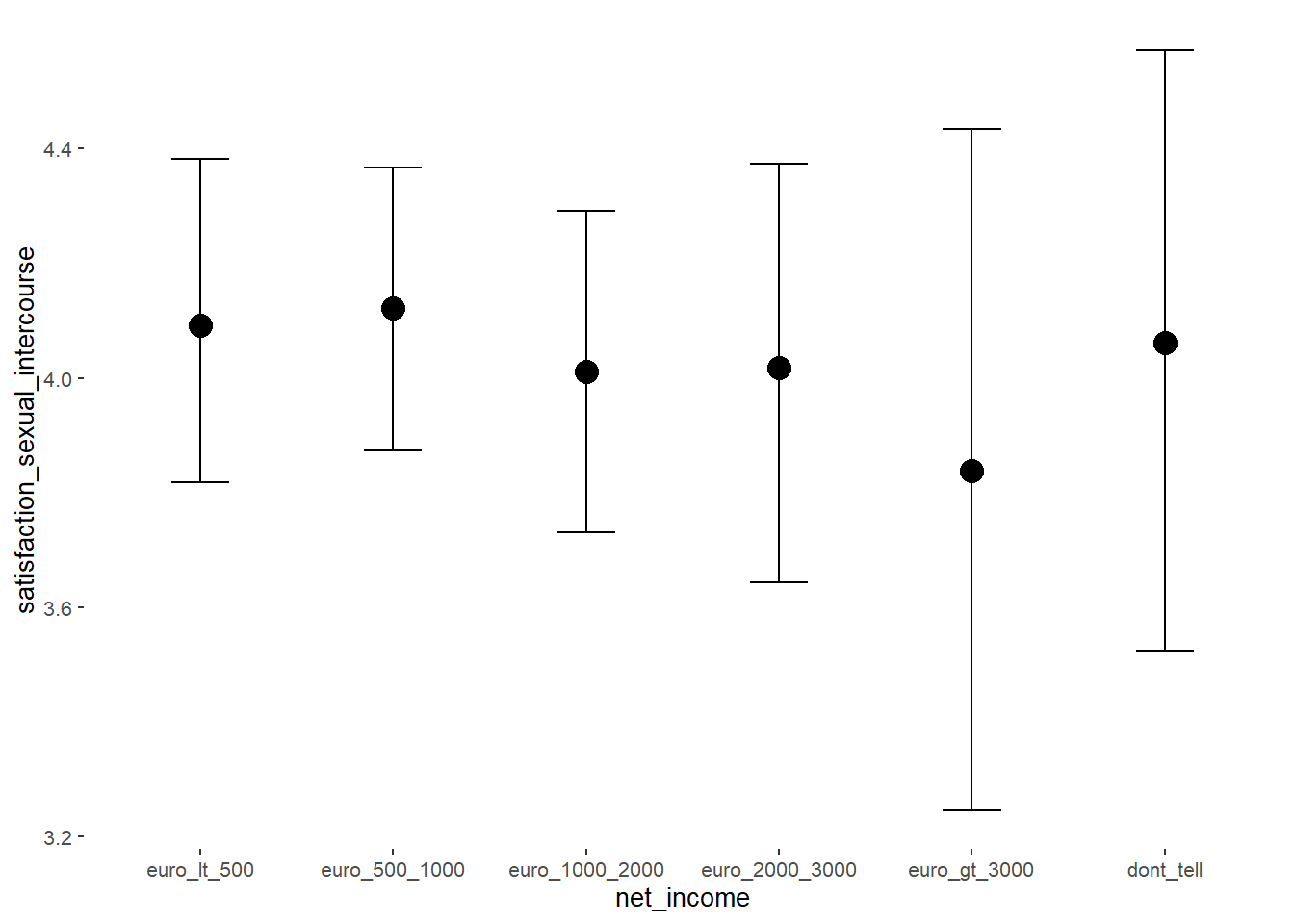
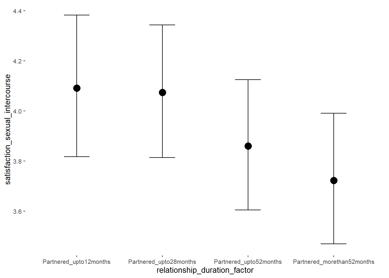
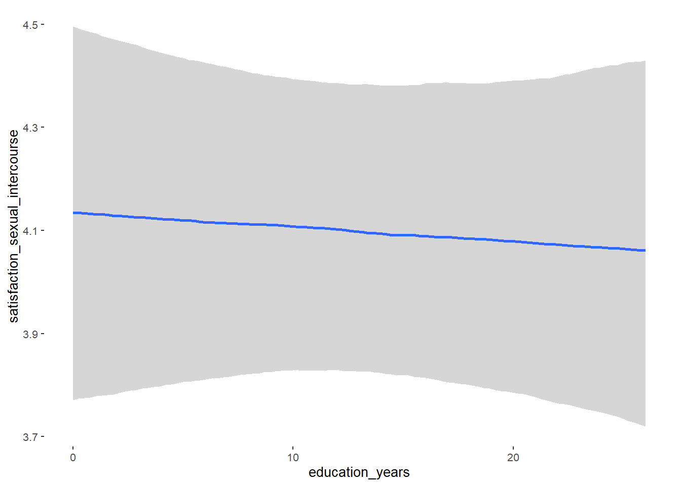
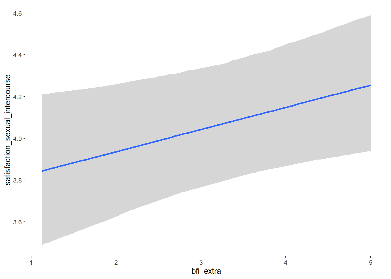
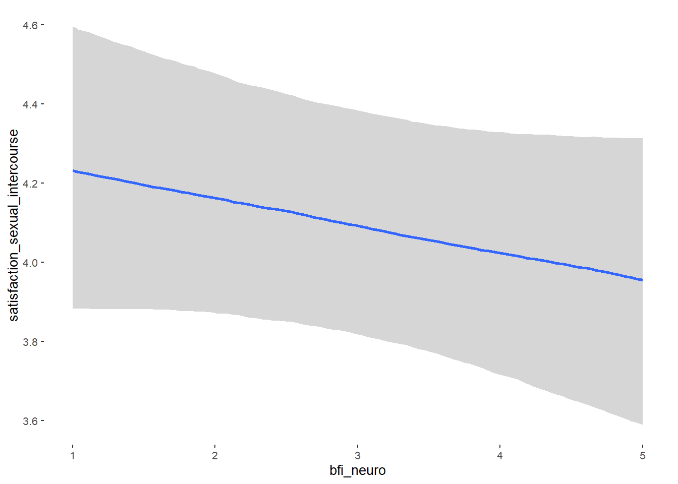
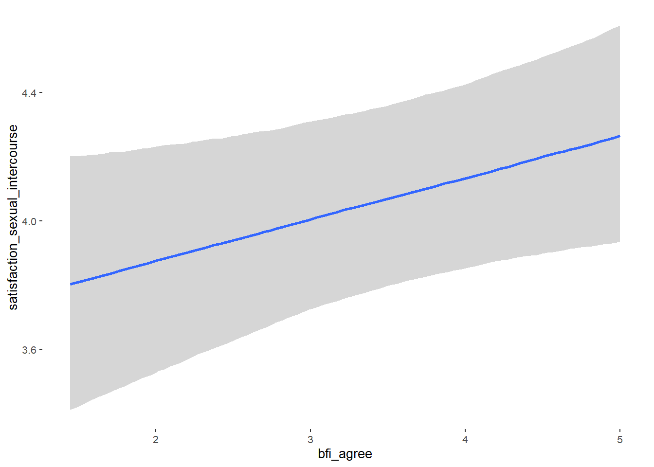
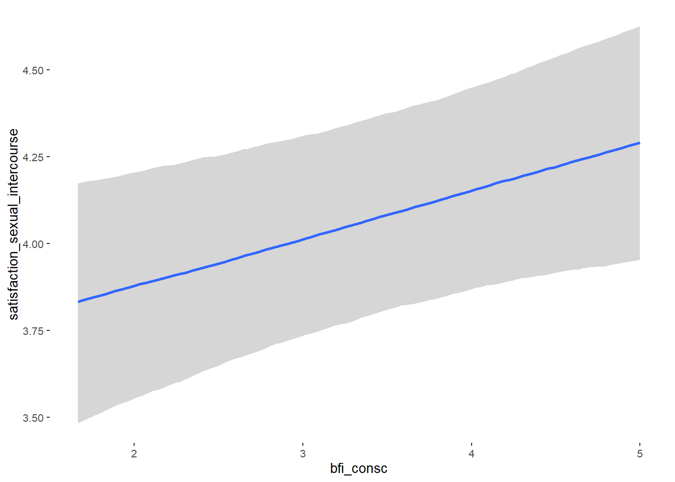
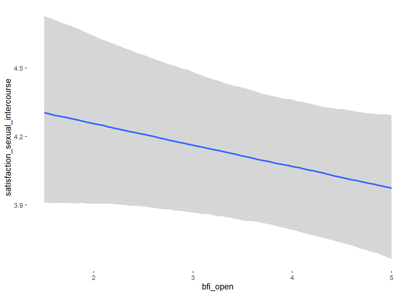
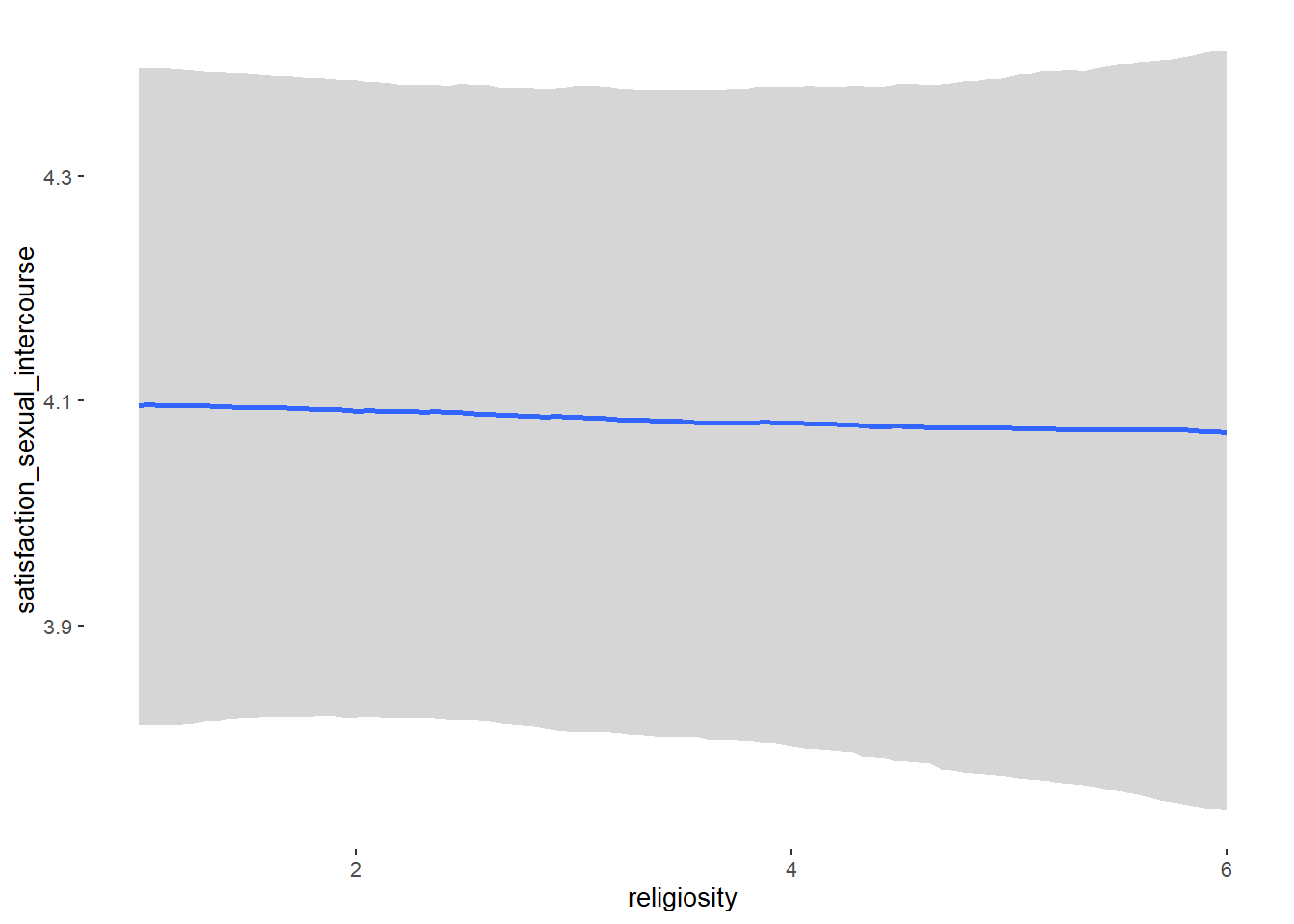
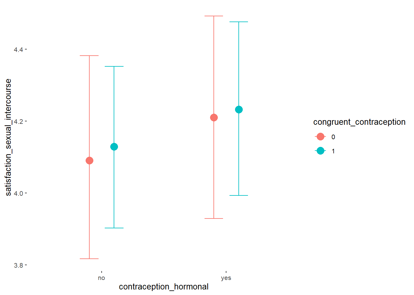
Forest Plot for Effect Sizes
m_congruency_sexsat_controlled %>%

  spread_draws(b_contraception_hormonalyes, b_congruent_contraception1,
               `b_contraception_hormonalyes:congruent_contraception1`,
               b_age,
               b_net_incomeeuro_500_1000, b_net_incomeeuro_1000_2000,
               b_net_incomeeuro_2000_3000, b_net_incomeeuro_gt_3000, b_net_incomedont_tell,
               b_relationship_duration_factorPartnered_upto28months,
               b_relationship_duration_factorPartnered_upto52months,
               b_relationship_duration_factorPartnered_morethan52months,
               b_education_years,
               b_bfi_extra, b_bfi_neuro, b_bfi_agree, b_bfi_consc, b_bfi_open,
               b_religiosity) %>%
  pivot_longer(cols = c(b_contraception_hormonalyes, b_congruent_contraception1,
               `b_contraception_hormonalyes:congruent_contraception1`,
                        b_age,
               b_net_incomeeuro_500_1000, b_net_incomeeuro_1000_2000,
               b_net_incomeeuro_2000_3000, b_net_incomeeuro_gt_3000, b_net_incomedont_tell,
               b_relationship_duration_factorPartnered_upto28months,
               b_relationship_duration_factorPartnered_upto52months,
               b_relationship_duration_factorPartnered_morethan52months,
               b_education_years,
               b_bfi_extra, b_bfi_neuro, b_bfi_agree, b_bfi_consc, b_bfi_open,
               b_religiosity),
               names_to = "condition",
               values_to = "r_condition") %>%
  mutate(condition_mean = r_condition,
         group = ifelse(condition %contains% "b_relationship_duration_factor",
                        "Relationship Duration",
                        ifelse(condition %contains% "b_net_income",
                               "Income",
                               NA)),
         group = ifelse(condition %contains% "ontraception",
                        "Contraception", group),
         condition = ifelse(condition == "b_contraception_hormonalyes",
                        "Hormonal Contraception",
                     ifelse(condition == "b_congruent_contraception1",
                            "Congruent Contraception",
                     ifelse(condition == "b_contraception_hormonalyes:congruent_contraception1",
                            "Interaction Hormonal Contracpetion and Congruent Contraception",
                            condition))),
         condition = ifelse(condition == "b_age", "Age",
                ifelse(condition == "b_net_incomeeuro_500_1000", "500-1000 Euro",
                ifelse(condition == "b_net_incomeeuro_1000_2000", "1000-2000 Euro",
                ifelse(condition == "b_net_incomeeuro_2000_3000", "2000-3000 Euro",
                ifelse(condition == "b_net_incomeeuro_gt_3000", ">3000 Euro",
                ifelse(condition == "b_net_incomedont_tell", "do not tell",
                ifelse(condition == "b_relationship_duration_factorPartnered_upto28months",
                       "13-28 months",
                ifelse(condition == "b_relationship_duration_factorPartnered_upto52months",
                       "29-52 months",
                ifelse(condition == "b_relationship_duration_factorPartnered_morethan52months",
                       ">52 months",
                ifelse(condition == "b_education_years", "Years of Education",
                ifelse(condition == "b_bfi_extra", "Extraversion",
                ifelse(condition == "b_bfi_neuro", "Neuroticism",
                ifelse(condition == "b_bfi_agree", "Agreeableness",
                ifelse(condition == "b_bfi_consc", "Conscientiousness",
                ifelse(condition == "b_bfi_open", "Openness",
                ifelse(condition == "b_religiosity", "Religiosity",
                       condition)))))))))))))))),
         group = ifelse(is.na(group), condition, group),
         condition = factor(condition, levels = rev(c("Hormonal Contraception",
                                        "Congruent Contraception",
                                        "Interaction Hormonal Contracpetion and Congruent Contraception",
                                        "Age",
                                        "500-1000 Euro", "1000-2000 Euro",
                                        "2000-3000 Euro", ">3000 Euro", "do not tell",
                                        "13-28 months", "29-52 months",
                                        ">52 months",
                                        "Years of Education",
                                        "Extraversion", "Neuroticism", "Agreeableness",
                                         "Conscientiousness","Openness","Religiosity"))),
         group = factor(group, levels = c("Contraception", "Age", "Income",
                                          "Relationship Duration","Years of Education",
                                          "Extraversion", "Neuroticism", "Agreeableness",
                                         "Conscientiousness","Openness","Religiosity"))) %>%
  ggplot(aes(y = condition,
             x = condition_mean,
             fill = stat(abs(x) < 0.11))) +
  stat_halfeye() +
  geom_vline(xintercept = c(-0.11, 0.11), linetype = "dotted") +
  apatheme +
  theme(legend.position = "none") +
  scale_fill_manual(values = c("gray80", "skyblue")) +
  labs(x = "Effect Size Estimates", y = "Predictors")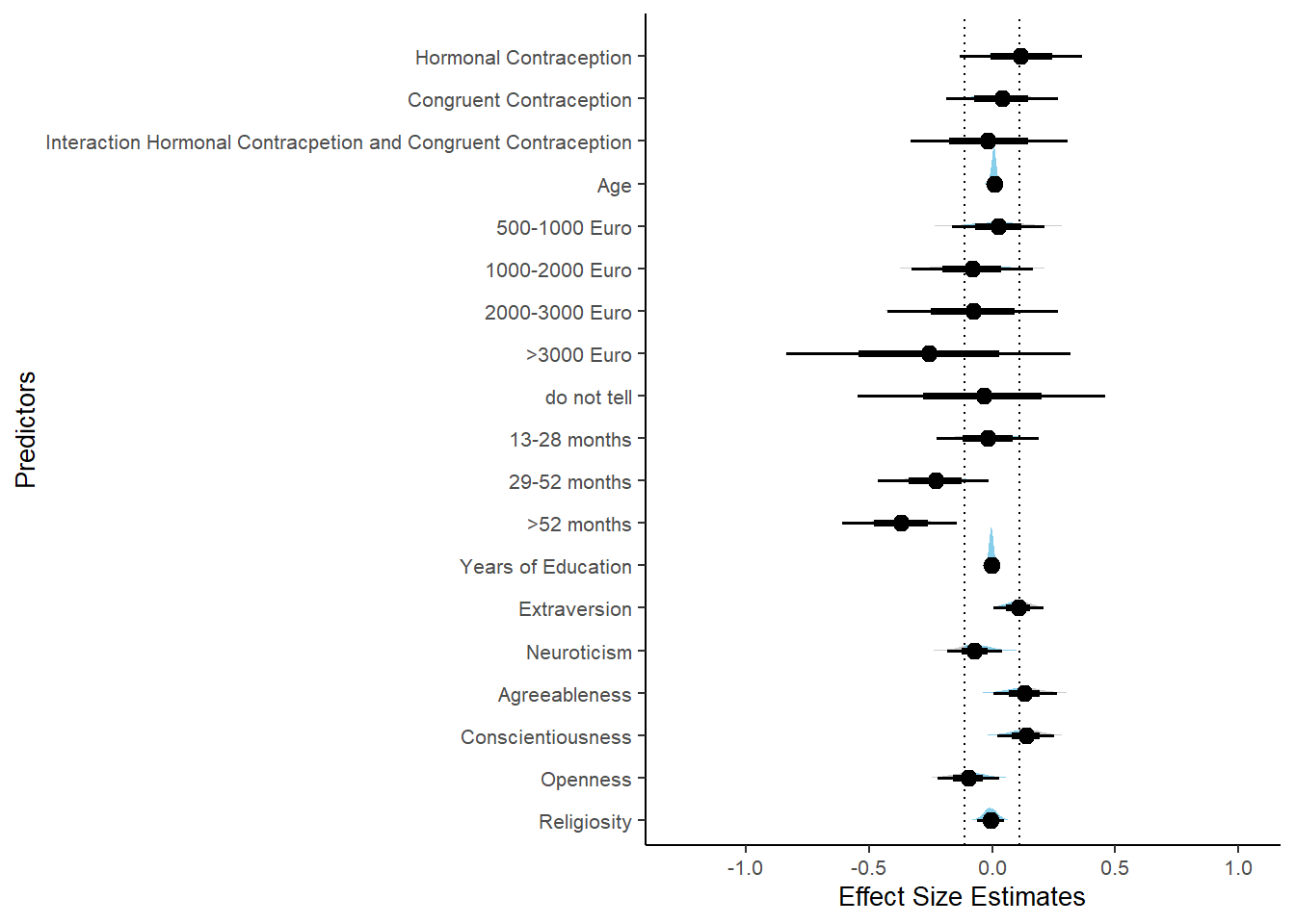
Libido
Model
m_congruency_libido_controlled = brm(diary_libido_mean ~
                          contraception_hormonal * congruent_contraception +
                             age + net_income + relationship_duration_factor +
                              education_years +
                              bfi_extra + bfi_neuro + bfi_agree + bfi_consc + bfi_open +
                              religiosity,
                data = data, family = gaussian(),
                file = "m_congruency_libido_controlled")
Summary
##  Family: gaussian
##   Links: mu = identity; sigma = identity
## Formula: diary_libido_mean ~ contraception_hormonal * congruent_contraception + age + net_income + relationship_duration_factor + education_years + bfi_extra + bfi_neuro + bfi_agree + bfi_consc + bfi_open + religiosity
##    Data: data (Number of observations: 632)
##   Draws: 4 chains, each with iter = 2000; warmup = 1000; thin = 1;
##          total post-warmup draws = 4000
##
## Population-Level Effects:
##                                                        Estimate Est.Error l-90% CI u-90% CI Rhat Bulk_ESS
## Intercept                                                  1.07      0.31     0.57     1.60 1.00     5382
## contraception_hormonalyes                                 -0.02      0.07    -0.14     0.11 1.00     3571
## congruent_contraception1                                   0.02      0.06    -0.09     0.12 1.00     3601
## age                                                       -0.00      0.01    -0.01     0.00 1.00     4007
## net_incomeeuro_500_1000                                    0.12      0.05     0.03     0.21 1.00     3657
## net_incomeeuro_1000_2000                                   0.14      0.07     0.02     0.27 1.00     3164
## net_incomeeuro_2000_3000                                   0.14      0.10    -0.04     0.30 1.00     3487
## net_incomeeuro_gt_3000                                     0.02      0.18    -0.29     0.32 1.00     4150
## net_incomedont_tell                                        0.27      0.14     0.03     0.50 1.00     4255
## relationship_duration_factorPartnered_upto28months        -0.11      0.06    -0.21    -0.02 1.00     3842
## relationship_duration_factorPartnered_upto52months        -0.15      0.07    -0.26    -0.04 1.00     3830
## relationship_duration_factorPartnered_morethan52months    -0.18      0.07    -0.29    -0.06 1.00     3838
## education_years                                           -0.00      0.00    -0.01     0.01 1.00     5899
## bfi_extra                                                  0.06      0.03     0.01     0.11 1.00     4656
## bfi_neuro                                                 -0.03      0.03    -0.08     0.03 1.00     4337
## bfi_agree                                                  0.07      0.04     0.01     0.13 1.00     4542
## bfi_consc                                                 -0.09      0.03    -0.15    -0.04 1.00     5385
## bfi_open                                                   0.09      0.04     0.03     0.15 1.00     5544
## religiosity                                               -0.00      0.02    -0.03     0.02 1.00     5039
## contraception_hormonalyes:congruent_contraception1         0.04      0.09    -0.11     0.19 1.00     3167
##                                                        Tail_ESS
## Intercept                                                  3690
## contraception_hormonalyes                                  2734
## congruent_contraception1                                   3274
## age                                                        3216
## net_incomeeuro_500_1000                                    3272
## net_incomeeuro_1000_2000                                   2914
## net_incomeeuro_2000_3000                                   2962
## net_incomeeuro_gt_3000                                     2800
## net_incomedont_tell                                        2891
## relationship_duration_factorPartnered_upto28months         3163
## relationship_duration_factorPartnered_upto52months         3268
## relationship_duration_factorPartnered_morethan52months     3337
## education_years                                            3177
## bfi_extra                                                  3376
## bfi_neuro                                                  3014
## bfi_agree                                                  3185
## bfi_consc                                                  3310
## bfi_open                                                   3153
## religiosity                                                3107
## contraception_hormonalyes:congruent_contraception1         2743
##
## Family Specific Parameters:
##       Estimate Est.Error l-90% CI u-90% CI Rhat Bulk_ESS Tail_ESS
## sigma     0.53      0.02     0.51     0.56 1.00     4580     2911
##
## Draws were sampled using sampling(NUTS). For each parameter, Bulk_ESS
## and Tail_ESS are effective sample size measures, and Rhat is the potential
## scale reduction factor on split chains (at convergence, Rhat = 1).
Comparison with ROPE
plot(equivalence_test(m_congruency_libido_controlled, range = c(-0.06, 0.06), ci = 0.90,
                      parameters = "contraception"))
## Possible multicollinearity between b_contraception_hormonalyes:congruent_contraception1 and b_contraception_hormonalyes (r = 0.79). This might lead to inappropriate results. See 'Details' in '?equivalence_test'.## Picking joint bandwidth of 0.0105## Warning: Removed 1197 rows containing non-finite values (stat_density_ridges).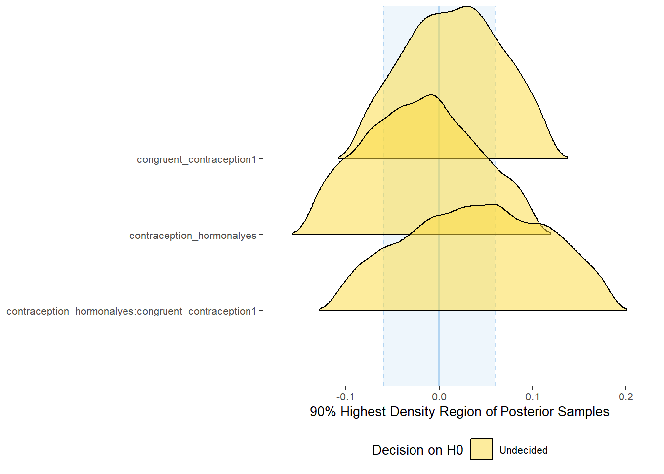
equivalence_test(m_congruency_libido_controlled, range = c(-0.06, 0.06), ci = 0.90,
                      parameters = "contraception")
## Possible multicollinearity between b_contraception_hormonalyes:congruent_contraception1 and b_contraception_hormonalyes (r = 0.79). This might lead to inappropriate results. See 'Details' in '?equivalence_test'.## # A tibble: 3 x 10
## Parameter CI ROPE_low ROPE_high ROPE_Percentage ROPE_Equivalence HDI_low HDI_high Effects Component
## <chr> <dbl> <dbl> <dbl> <dbl> <chr> <dbl> <dbl> <chr> <chr>
## 1 b_contraceptio~ 0.9 -0.06 0.06 0.629 Undecided -0.138 0.102 fixed conditio~
## 2 b_congruent_co~ 0.9 -0.06 0.06 0.715 Undecided -0.0899 0.117 fixed conditio~
## 3 b_contraceptio~ 0.9 -0.06 0.06 0.490 Undecided -0.111 0.183 fixed conditio~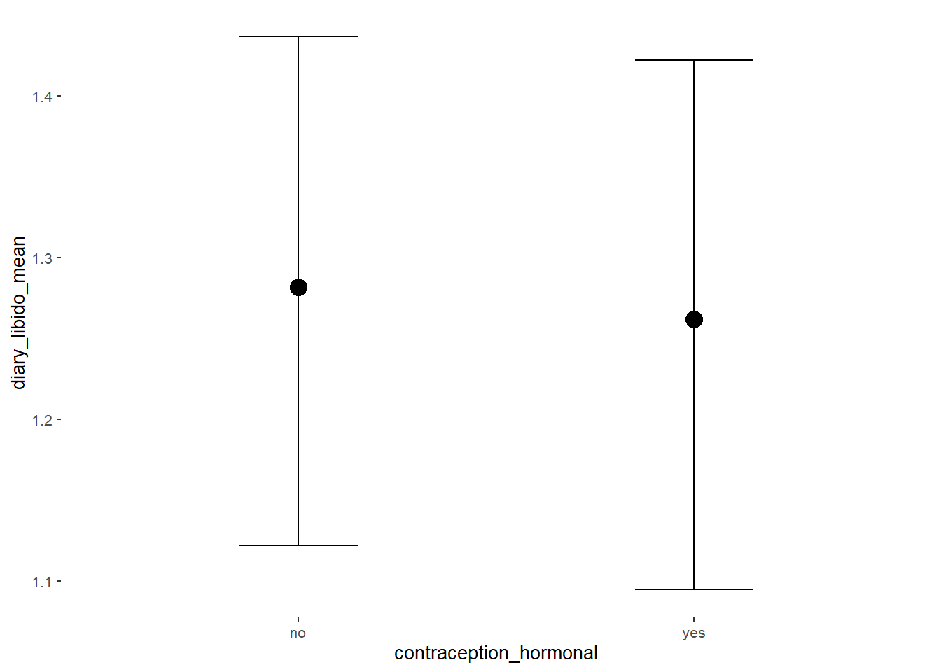
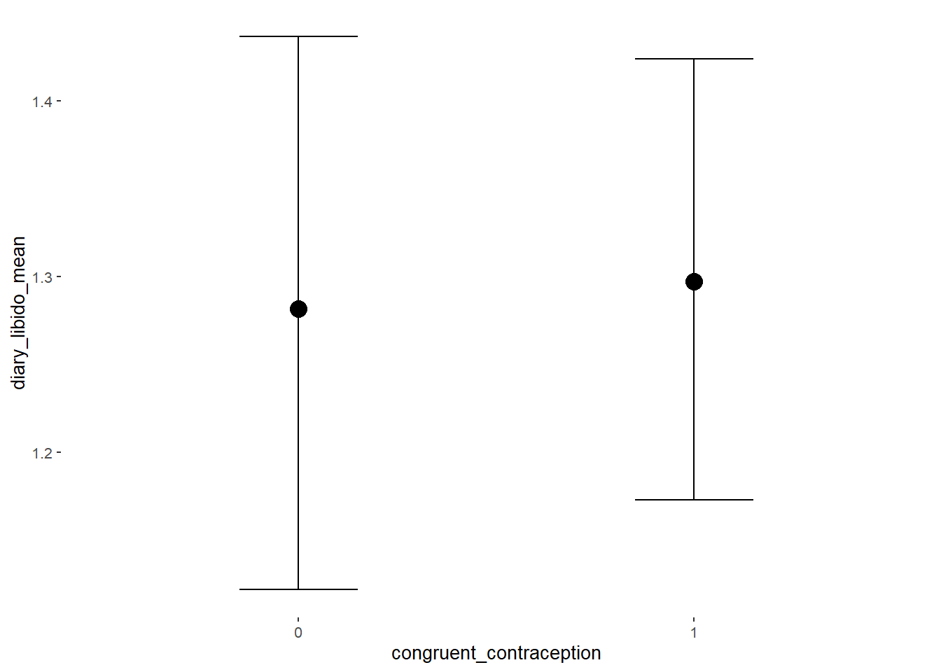
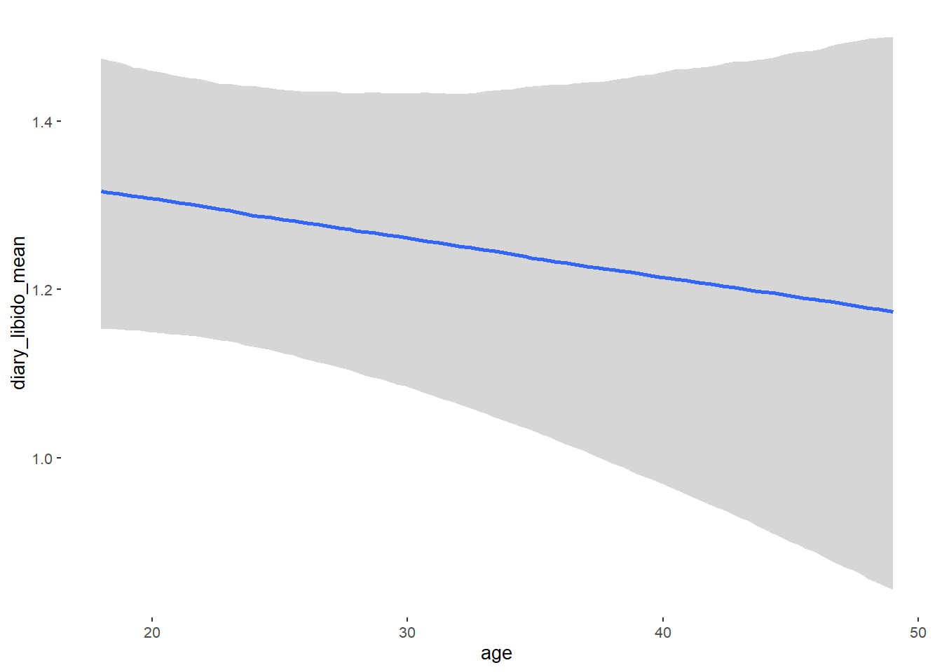
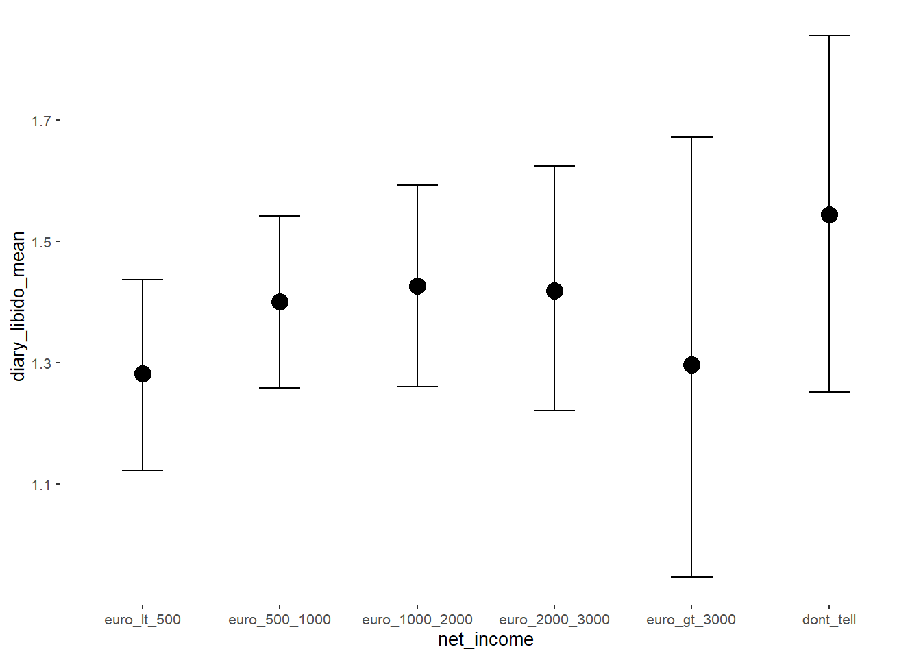
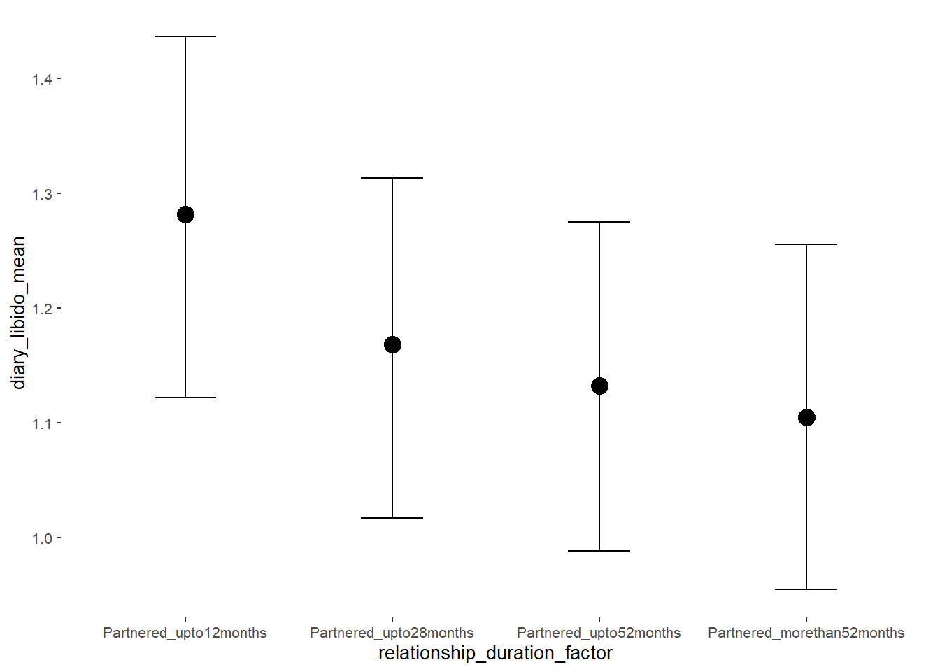
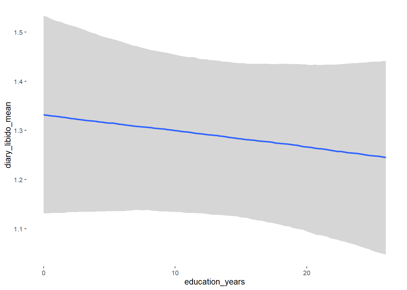
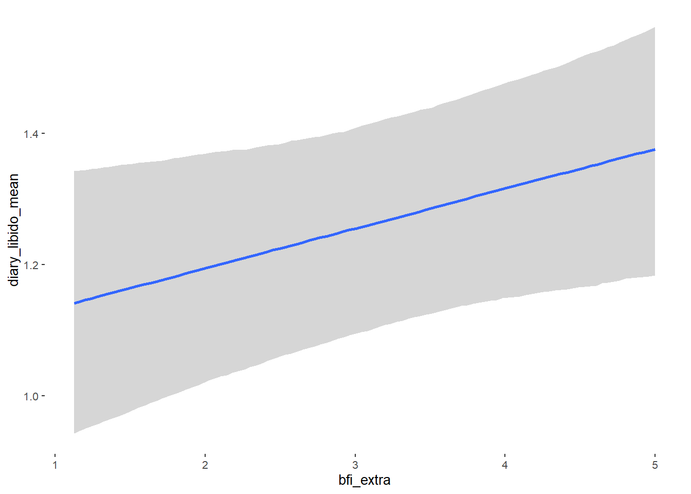
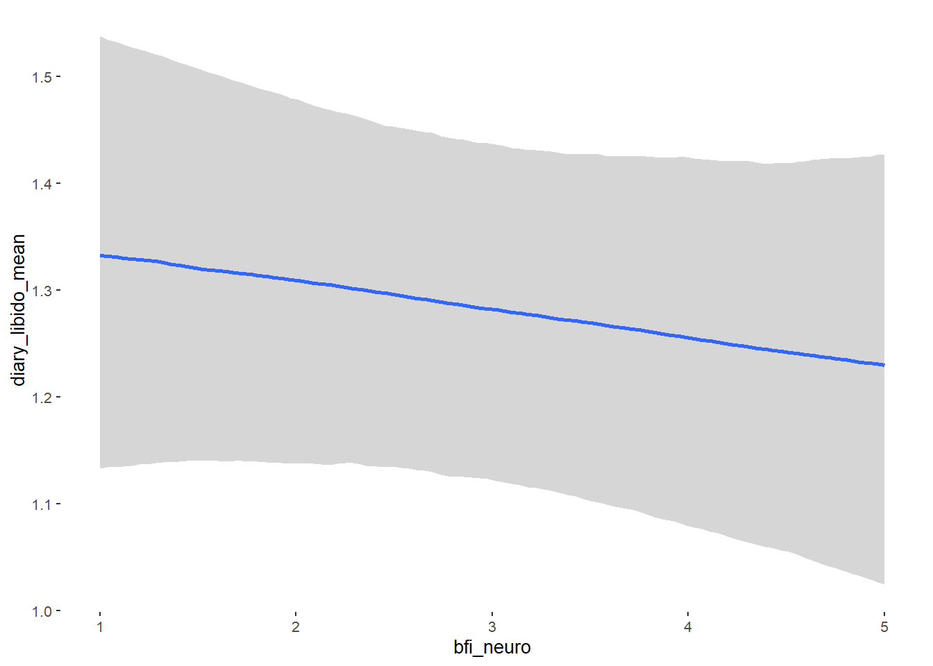
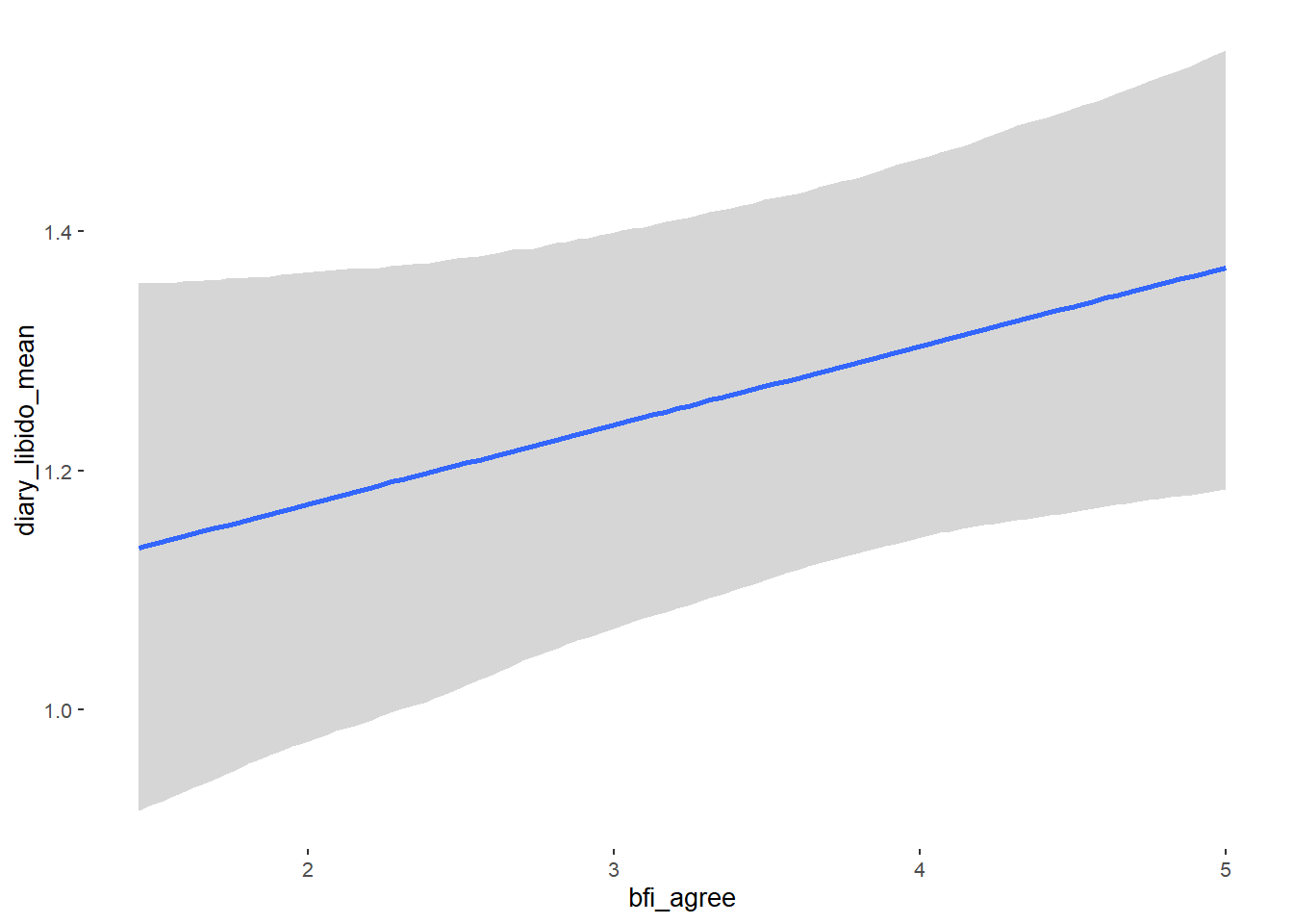
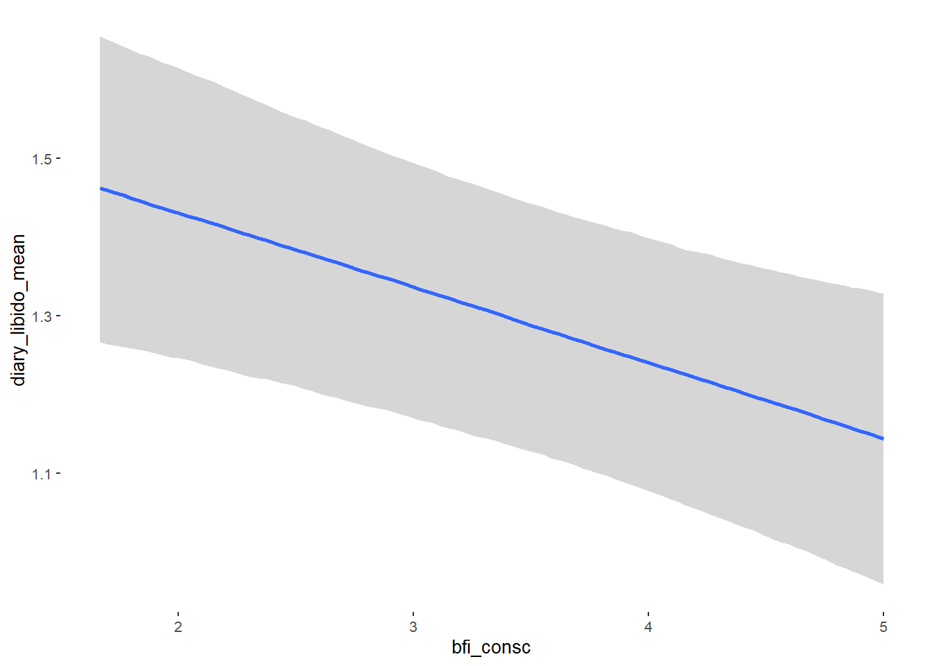
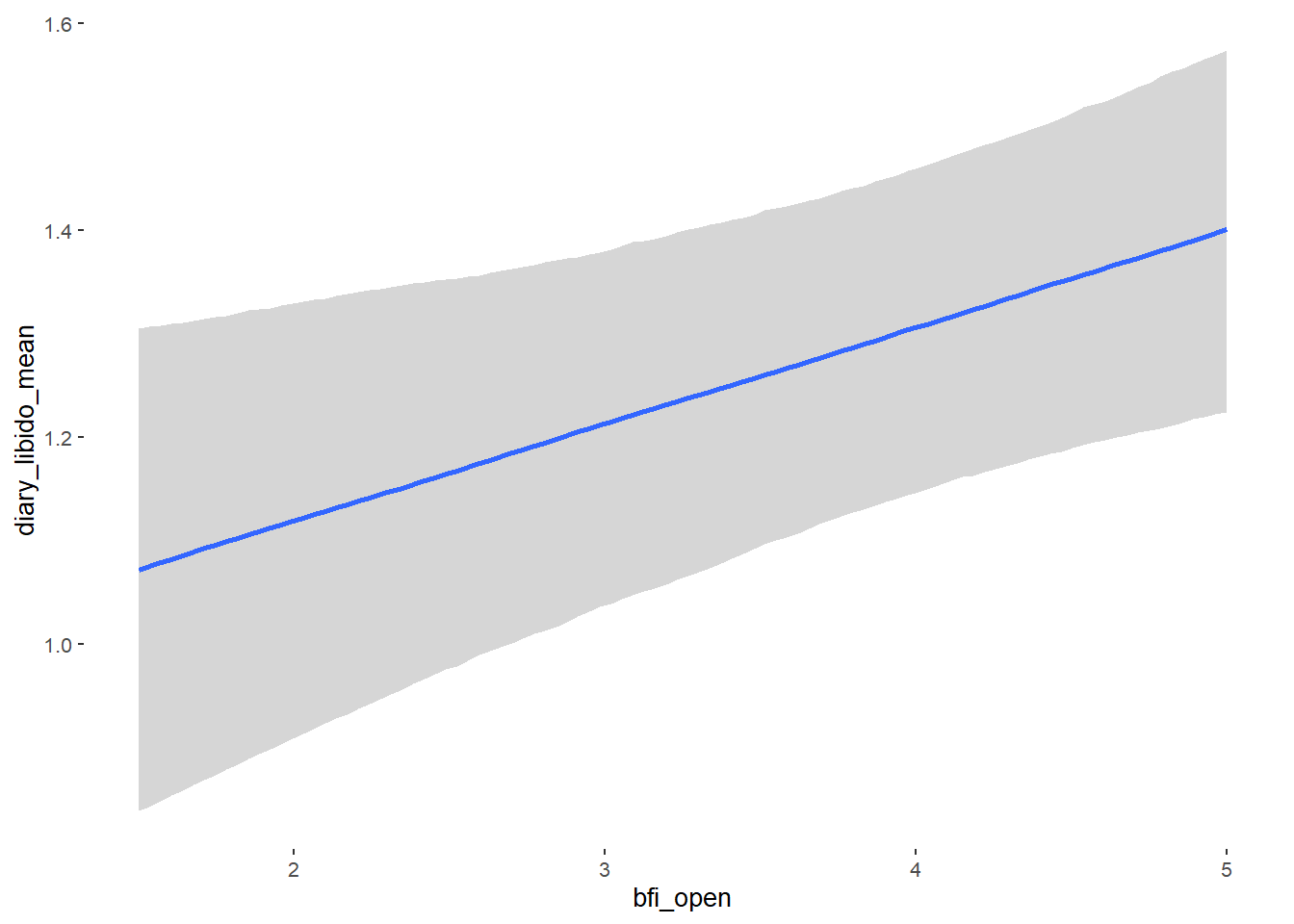
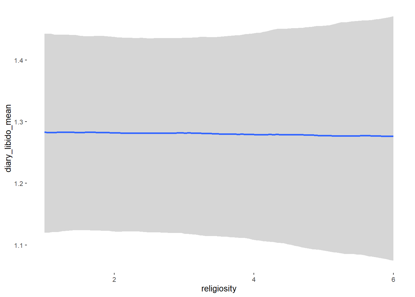
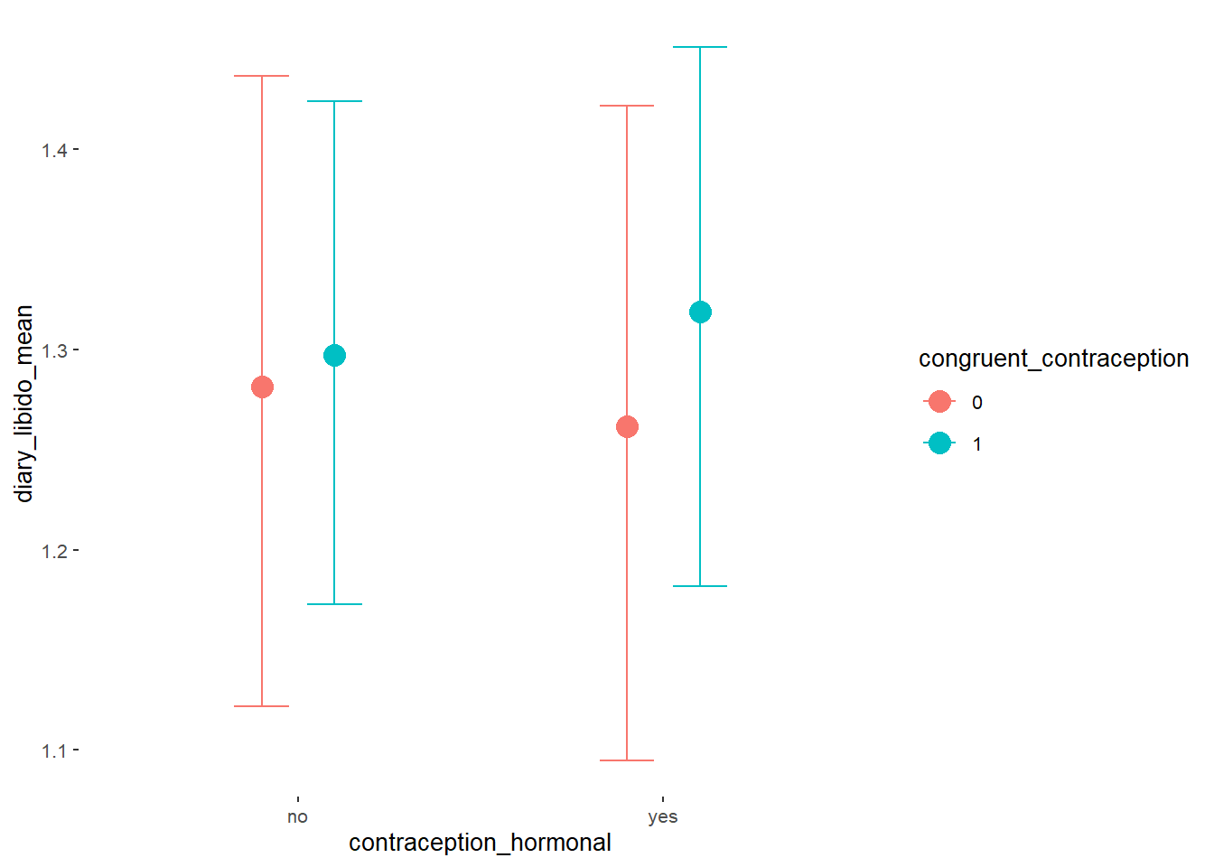
Forest Plot for Effect Sizes
m_congruency_libido_controlled %>%

  spread_draws(b_contraception_hormonalyes, b_congruent_contraception1,
               `b_contraception_hormonalyes:congruent_contraception1`,
               b_age,
               b_net_incomeeuro_500_1000, b_net_incomeeuro_1000_2000,
               b_net_incomeeuro_2000_3000, b_net_incomeeuro_gt_3000, b_net_incomedont_tell,
               b_relationship_duration_factorPartnered_upto28months,
               b_relationship_duration_factorPartnered_upto52months,
               b_relationship_duration_factorPartnered_morethan52months,
               b_education_years,
               b_bfi_extra, b_bfi_neuro, b_bfi_agree, b_bfi_consc, b_bfi_open,
               b_religiosity) %>%
  pivot_longer(cols = c(b_contraception_hormonalyes, b_congruent_contraception1,
               `b_contraception_hormonalyes:congruent_contraception1`,
                        b_age,
               b_net_incomeeuro_500_1000, b_net_incomeeuro_1000_2000,
               b_net_incomeeuro_2000_3000, b_net_incomeeuro_gt_3000, b_net_incomedont_tell,
               b_relationship_duration_factorPartnered_upto28months,
               b_relationship_duration_factorPartnered_upto52months,
               b_relationship_duration_factorPartnered_morethan52months,
               b_education_years,
               b_bfi_extra, b_bfi_neuro, b_bfi_agree, b_bfi_consc, b_bfi_open,
               b_religiosity),
               names_to = "condition",
               values_to = "r_condition") %>%
  mutate(condition_mean = r_condition,
         group = ifelse(condition %contains% "b_relationship_duration_factor",
                        "Relationship Duration",
                        ifelse(condition %contains% "b_net_income",
                               "Income",
                               NA)),
         group = ifelse(condition %contains% "ontraception",
                        "Contraception", group),
         condition = ifelse(condition == "b_contraception_hormonalyes",
                        "Hormonal Contraception",
                     ifelse(condition == "b_congruent_contraception1",
                            "Congruent Contraception",
                     ifelse(condition == "b_contraception_hormonalyes:congruent_contraception1",
                            "Interaction Hormonal Contracpetion and Congruent Contraception",
                            condition))),
         condition = ifelse(condition == "b_age", "Age",
                ifelse(condition == "b_net_incomeeuro_500_1000", "500-1000 Euro",
                ifelse(condition == "b_net_incomeeuro_1000_2000", "1000-2000 Euro",
                ifelse(condition == "b_net_incomeeuro_2000_3000", "2000-3000 Euro",
                ifelse(condition == "b_net_incomeeuro_gt_3000", ">3000 Euro",
                ifelse(condition == "b_net_incomedont_tell", "do not tell",
                ifelse(condition == "b_relationship_duration_factorPartnered_upto28months",
                       "13-28 months",
                ifelse(condition == "b_relationship_duration_factorPartnered_upto52months",
                       "29-52 months",
                ifelse(condition == "b_relationship_duration_factorPartnered_morethan52months",
                       ">52 months",
                ifelse(condition == "b_education_years", "Years of Education",
                ifelse(condition == "b_bfi_extra", "Extraversion",
                ifelse(condition == "b_bfi_neuro", "Neuroticism",
                ifelse(condition == "b_bfi_agree", "Agreeableness",
                ifelse(condition == "b_bfi_consc", "Conscientiousness",
                ifelse(condition == "b_bfi_open", "Openness",
                ifelse(condition == "b_religiosity", "Religiosity",
                       condition)))))))))))))))),
         group = ifelse(is.na(group), condition, group),
         condition = factor(condition, levels = rev(c("Hormonal Contraception",
                                        "Congruent Contraception",
                                        "Interaction Hormonal Contracpetion and Congruent Contraception",
                                        "Age",
                                        "500-1000 Euro", "1000-2000 Euro",
                                        "2000-3000 Euro", ">3000 Euro", "do not tell",
                                        "13-28 months", "29-52 months",
                                        ">52 months",
                                        "Years of Education",
                                        "Extraversion", "Neuroticism", "Agreeableness",
                                         "Conscientiousness","Openness","Religiosity"))),
         group = factor(group, levels = c("Contraception", "Age", "Income",
                                          "Relationship Duration","Years of Education",
                                          "Extraversion", "Neuroticism", "Agreeableness",
                                         "Conscientiousness","Openness","Religiosity"))) %>%
  ggplot(aes(y = condition,
             x = condition_mean,
             fill = stat(abs(x) < 0.06))) +
  stat_halfeye() +
  geom_vline(xintercept = c(-0.06, 0.06), linetype = "dotted") +
  apatheme +
  theme(legend.position = "none") +
  scale_fill_manual(values = c("gray80", "skyblue")) +
  labs(x = "Effect Size Estimates", y = "Predictors")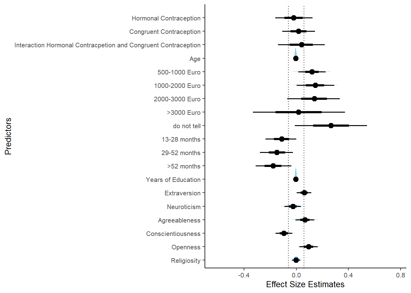
Sexual Frequency (Penetrative Intercourse)
Model
m_congruency_sexfreqpen_controlled = brm(diary_sex_active_sex_sum ~
                        offset(log(number_of_days)) +
                        contraception_hormonal * congruent_contraception +
                        age + net_income + relationship_duration_factor +
                              education_years +
                              bfi_extra + bfi_neuro + bfi_agree + bfi_consc + bfi_open +
                              religiosity,
                data = data, family = poisson(),
                file = "m_congruency_sexfreqpen_controlled")
## Warning: Rows containing NAs were excluded from the model.## Compiling Stan program...## recompiling to avoid crashing R session## Start sampling##
## SAMPLING FOR MODEL 'c63cc6f90adde557ca52c07be9ae7367' NOW (CHAIN 1).
## Chain 1:
## Chain 1: Gradient evaluation took 0 seconds
## Chain 1: 1000 transitions using 10 leapfrog steps per transition would take 0 seconds.
## Chain 1: Adjust your expectations accordingly!
## Chain 1:
## Chain 1:
## Chain 1: Iteration: 1 / 2000 [ 0%] (Warmup)
## Chain 1: Iteration: 200 / 2000 [ 10%] (Warmup)
## Chain 1: Iteration: 400 / 2000 [ 20%] (Warmup)
## Chain 1: Iteration: 600 / 2000 [ 30%] (Warmup)
## Chain 1: Iteration: 800 / 2000 [ 40%] (Warmup)
## Chain 1: Iteration: 1000 / 2000 [ 50%] (Warmup)
## Chain 1: Iteration: 1001 / 2000 [ 50%] (Sampling)
## Chain 1: Iteration: 1200 / 2000 [ 60%] (Sampling)
## Chain 1: Iteration: 1400 / 2000 [ 70%] (Sampling)
## Chain 1: Iteration: 1600 / 2000 [ 80%] (Sampling)
## Chain 1: Iteration: 1800 / 2000 [ 90%] (Sampling)
## Chain 1: Iteration: 2000 / 2000 [100%] (Sampling)
## Chain 1:
## Chain 1: Elapsed Time: 91.036 seconds (Warm-up)
## Chain 1: 115.326 seconds (Sampling)
## Chain 1: 206.362 seconds (Total)
## Chain 1:
##
## SAMPLING FOR MODEL 'c63cc6f90adde557ca52c07be9ae7367' NOW (CHAIN 2).
## Chain 2:
## Chain 2: Gradient evaluation took 0 seconds
## Chain 2: 1000 transitions using 10 leapfrog steps per transition would take 0 seconds.
## Chain 2: Adjust your expectations accordingly!
## Chain 2:
## Chain 2:
## Chain 2: Iteration: 1 / 2000 [ 0%] (Warmup)
## Chain 2: Iteration: 200 / 2000 [ 10%] (Warmup)
## Chain 2: Iteration: 400 / 2000 [ 20%] (Warmup)
## Chain 2: Iteration: 600 / 2000 [ 30%] (Warmup)
## Chain 2: Iteration: 800 / 2000 [ 40%] (Warmup)
## Chain 2: Iteration: 1000 / 2000 [ 50%] (Warmup)
## Chain 2: Iteration: 1001 / 2000 [ 50%] (Sampling)
## Chain 2: Iteration: 1200 / 2000 [ 60%] (Sampling)
## Chain 2: Iteration: 1400 / 2000 [ 70%] (Sampling)
## Chain 2: Iteration: 1600 / 2000 [ 80%] (Sampling)
## Chain 2: Iteration: 1800 / 2000 [ 90%] (Sampling)
## Chain 2: Iteration: 2000 / 2000 [100%] (Sampling)
## Chain 2:
## Chain 2: Elapsed Time: 96.757 seconds (Warm-up)
## Chain 2: 114.862 seconds (Sampling)
## Chain 2: 211.619 seconds (Total)
## Chain 2:
##
## SAMPLING FOR MODEL 'c63cc6f90adde557ca52c07be9ae7367' NOW (CHAIN 3).
## Chain 3:
## Chain 3: Gradient evaluation took 0 seconds
## Chain 3: 1000 transitions using 10 leapfrog steps per transition would take 0 seconds.
## Chain 3: Adjust your expectations accordingly!
## Chain 3:
## Chain 3:
## Chain 3: Iteration: 1 / 2000 [ 0%] (Warmup)
## Chain 3: Iteration: 200 / 2000 [ 10%] (Warmup)
## Chain 3: Iteration: 400 / 2000 [ 20%] (Warmup)
## Chain 3: Iteration: 600 / 2000 [ 30%] (Warmup)
## Chain 3: Iteration: 800 / 2000 [ 40%] (Warmup)
## Chain 3: Iteration: 1000 / 2000 [ 50%] (Warmup)
## Chain 3: Iteration: 1001 / 2000 [ 50%] (Sampling)
## Chain 3: Iteration: 1200 / 2000 [ 60%] (Sampling)
## Chain 3: Iteration: 1400 / 2000 [ 70%] (Sampling)
## Chain 3: Iteration: 1600 / 2000 [ 80%] (Sampling)
## Chain 3: Iteration: 1800 / 2000 [ 90%] (Sampling)
## Chain 3: Iteration: 2000 / 2000 [100%] (Sampling)
## Chain 3:
## Chain 3: Elapsed Time: 94.349 seconds (Warm-up)
## Chain 3: 115.023 seconds (Sampling)
## Chain 3: 209.372 seconds (Total)
## Chain 3:
##
## SAMPLING FOR MODEL 'c63cc6f90adde557ca52c07be9ae7367' NOW (CHAIN 4).
## Chain 4:
## Chain 4: Gradient evaluation took 0 seconds
## Chain 4: 1000 transitions using 10 leapfrog steps per transition would take 0 seconds.
## Chain 4: Adjust your expectations accordingly!
## Chain 4:
## Chain 4:
## Chain 4: Iteration: 1 / 2000 [ 0%] (Warmup)
## Chain 4: Iteration: 200 / 2000 [ 10%] (Warmup)
## Chain 4: Iteration: 400 / 2000 [ 20%] (Warmup)
## Chain 4: Iteration: 600 / 2000 [ 30%] (Warmup)
## Chain 4: Iteration: 800 / 2000 [ 40%] (Warmup)
## Chain 4: Iteration: 1000 / 2000 [ 50%] (Warmup)
## Chain 4: Iteration: 1001 / 2000 [ 50%] (Sampling)
## Chain 4: Iteration: 1200 / 2000 [ 60%] (Sampling)
## Chain 4: Iteration: 1400 / 2000 [ 70%] (Sampling)
## Chain 4: Iteration: 1600 / 2000 [ 80%] (Sampling)
## Chain 4: Iteration: 1800 / 2000 [ 90%] (Sampling)
## Chain 4: Iteration: 2000 / 2000 [100%] (Sampling)
## Chain 4:
## Chain 4: Elapsed Time: 94.231 seconds (Warm-up)
## Chain 4: 114.17 seconds (Sampling)
## Chain 4: 208.401 seconds (Total)
## Chain 4:## Warning: There were 4000 transitions after warmup that exceeded the maximum treedepth. Increase max_treedepth above 10. See
## http://mc-stan.org/misc/warnings.html#maximum-treedepth-exceeded## Warning: Examine the pairs() plot to diagnose sampling problems## Warning: The largest R-hat is 2.87, indicating chains have not mixed.
## Running the chains for more iterations may help. See
## http://mc-stan.org/misc/warnings.html#r-hat## Warning: Bulk Effective Samples Size (ESS) is too low, indicating posterior means and medians may be unreliable.
## Running the chains for more iterations may help. See
## http://mc-stan.org/misc/warnings.html#bulk-ess## Warning: Tail Effective Samples Size (ESS) is too low, indicating posterior variances and tail quantiles may be unreliable.
## Running the chains for more iterations may help. See
## http://mc-stan.org/misc/warnings.html#tail-essSummary
## Warning: Parts of the model have not converged (some Rhats are > 1.05). Be careful when analysing the results!
## We recommend running more iterations and/or setting stronger priors.
## Family: poisson
## Links: mu = log
## Formula: diary_sex_active_sex_sum ~ offset(log(number_of_days)) + contraception_hormonal * congruent_contraception + age + net_income + relationship_duration_factor + education_years + bfi_extra + bfi_neuro + bfi_agree + bfi_consc + bfi_open + religiosity
## Data: data (Number of observations: 622)
## Draws: 4 chains, each with iter = 2000; warmup = 1000; thin = 1;
## total post-warmup draws = 4000
##
## Population-Level Effects:
## Estimate Est.Error l-90% CI u-90% CI Rhat Bulk_ESS
## Intercept 40.61 230.38 -280.16 358.71 2.87 5
## contraception_hormonalyes 0.14 0.05 0.06 0.22 1.14 39
## congruent_contraception1 -0.05 0.04 -0.11 0.01 1.08 40
## age -0.00 0.00 -0.01 0.00 1.06 52
## net_incomeeuro_500_1000 0.14 0.03 0.08 0.20 1.11 34
## net_incomeeuro_1000_2000 0.17 0.05 0.09 0.24 1.08 39
## net_incomeeuro_2000_3000 0.37 0.06 0.26 0.47 1.07 34
## net_incomeeuro_gt_3000 0.04 0.11 -0.16 0.19 1.14 29
## net_incomedont_tell 0.37 0.09 0.24 0.51 1.13 22
## relationship_duration_factorPartnered_upto12months -42.29 230.37 -360.31 278.53 2.87 5
## relationship_duration_factorPartnered_upto28months -42.42 230.37 -360.42 278.38 2.87 5
## relationship_duration_factorPartnered_upto52months -42.68 230.37 -360.71 278.12 2.87 5
## relationship_duration_factorPartnered_morethan52months -42.70 230.37 -360.69 278.13 2.87 5
## education_years -0.01 0.00 -0.01 -0.01 1.02 106
## bfi_extra -0.02 0.02 -0.05 0.01 1.14 26
## bfi_neuro -0.02 0.02 -0.05 0.01 1.19 19
## bfi_agree 0.09 0.02 0.06 0.13 1.05 47
## bfi_consc -0.03 0.02 -0.07 -0.00 1.24 14
## bfi_open 0.03 0.02 -0.00 0.07 1.08 40
## religiosity -0.01 0.01 -0.02 0.01 1.06 52
## contraception_hormonalyes:congruent_contraception1 0.05 0.06 -0.05 0.13 1.12 36
## Tail_ESS
## Intercept NA
## contraception_hormonalyes NA
## congruent_contraception1 NA
## age NA
## net_incomeeuro_500_1000 NA
## net_incomeeuro_1000_2000 NA
## net_incomeeuro_2000_3000 NA
## net_incomeeuro_gt_3000 NA
## net_incomedont_tell NA
## relationship_duration_factorPartnered_upto12months NA
## relationship_duration_factorPartnered_upto28months NA
## relationship_duration_factorPartnered_upto52months NA
## relationship_duration_factorPartnered_morethan52months NA
## education_years NA
## bfi_extra NA
## bfi_neuro NA
## bfi_agree NA
## bfi_consc NA
## bfi_open NA
## religiosity NA
## contraception_hormonalyes:congruent_contraception1 NA
##
## Draws were sampled using sampling(NUTS). For each parameter, Bulk_ESS
## and Tail_ESS are effective sample size measures, and Rhat is the potential
## scale reduction factor on split chains (at convergence, Rhat = 1).Comparison with ROPE
plot(equivalence_test(m_congruency_sexfreqpen_controlled, range = c(-0.05, 0.05),
                      ci = 0.90,
                      parameters = "contraception"))
## Possible multicollinearity between b_contraception_hormonalyes:congruent_contraception1 and b_contraception_hormonalyes (r = 0.79), b_contraception_hormonalyes:congruent_contraception1 and b_congruent_contraception1 (r = 0.73). This might lead to inappropriate results. See 'Details' in '?equivalence_test'.## Picking joint bandwidth of 0.00659## Warning: Removed 1197 rows containing non-finite values (stat_density_ridges).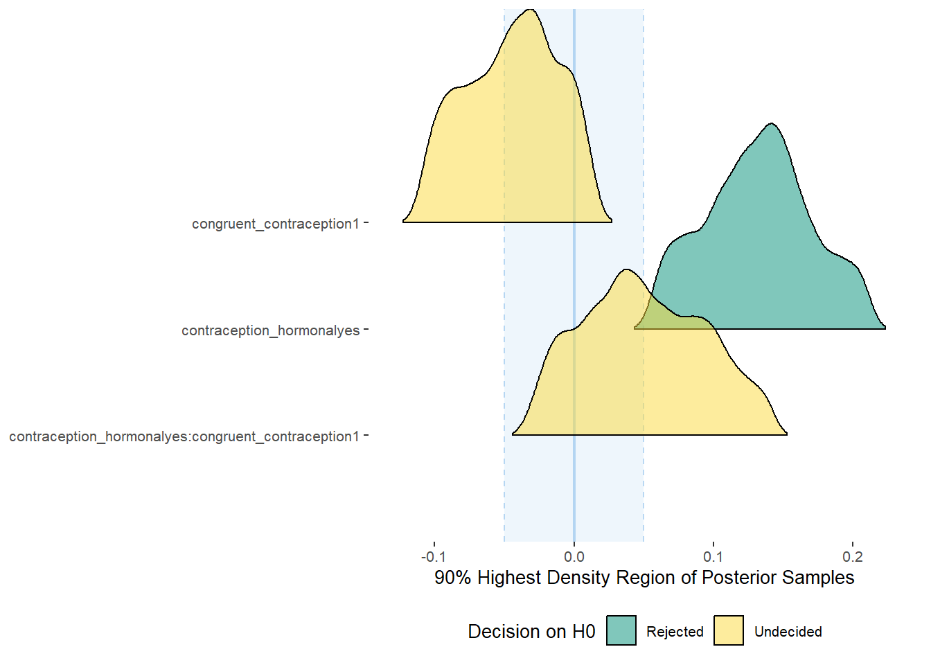
equivalence_test(m_congruency_sexfreqpen_controlled, range = c(-0.05, 0.05), ci = 0.90,
                      parameters = "contraception")
## Possible multicollinearity between b_contraception_hormonalyes:congruent_contraception1 and b_contraception_hormonalyes (r = 0.79), b_contraception_hormonalyes:congruent_contraception1 and b_congruent_contraception1 (r = 0.73). This might lead to inappropriate results. See 'Details' in '?equivalence_test'.## # A tibble: 3 x 10
## Parameter CI ROPE_low ROPE_high ROPE_Percentage ROPE_Equivalence HDI_low HDI_high Effects Component
## <chr> <dbl> <dbl> <dbl> <dbl> <chr> <dbl> <dbl> <chr> <chr>
## 1 b_contraceptio~ 0.9 -0.05 0.05 0 Rejected 0.0556 0.211 fixed conditio~
## 2 b_congruent_co~ 0.9 -0.05 0.05 0.581 Undecided -0.110 0.0144 fixed conditio~
## 3 b_contraceptio~ 0.9 -0.05 0.05 0.524 Undecided -0.0349 0.142 fixed conditio~Plots
conditional_effects(m_congruency_sexfreqpen_controlled,
                    effects = "contraception_hormonal:congruent_contraception",
                    conditions = data.frame(number_of_days = 1))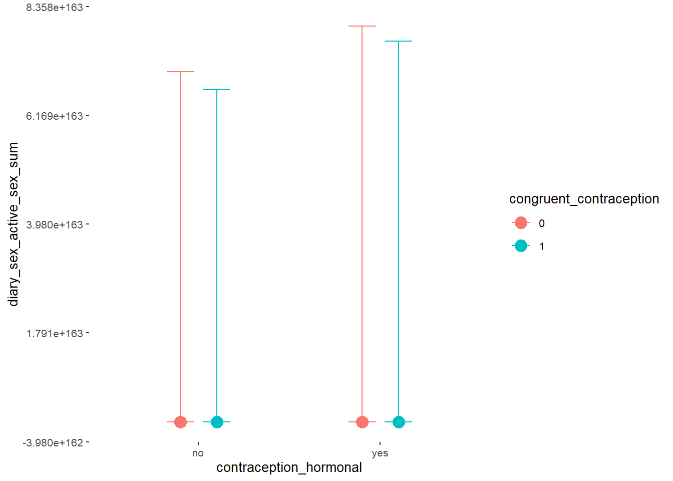
Forest Plot for Effect Sizes
m_congruency_sexfreqpen_controlled %>%

  spread_draws(b_contraception_hormonalyes, b_congruent_contraception1,
               `b_contraception_hormonalyes:congruent_contraception1`,
               b_age,
               b_net_incomeeuro_500_1000, b_net_incomeeuro_1000_2000,
               b_net_incomeeuro_2000_3000, b_net_incomeeuro_gt_3000, b_net_incomedont_tell,
               b_relationship_duration_factorPartnered_upto28months,
               b_relationship_duration_factorPartnered_upto52months,
               b_relationship_duration_factorPartnered_morethan52months,
               b_education_years,
               b_bfi_extra, b_bfi_neuro, b_bfi_agree, b_bfi_consc, b_bfi_open,
               b_religiosity) %>%
  pivot_longer(cols = c(b_contraception_hormonalyes, b_congruent_contraception1,
               `b_contraception_hormonalyes:congruent_contraception1`,
                        b_age,
               b_net_incomeeuro_500_1000, b_net_incomeeuro_1000_2000,
               b_net_incomeeuro_2000_3000, b_net_incomeeuro_gt_3000, b_net_incomedont_tell,
               b_relationship_duration_factorPartnered_upto28months,
               b_relationship_duration_factorPartnered_upto52months,
               b_relationship_duration_factorPartnered_morethan52months,
               b_education_years,
               b_bfi_extra, b_bfi_neuro, b_bfi_agree, b_bfi_consc, b_bfi_open,
               b_religiosity),
               names_to = "condition",
               values_to = "r_condition") %>%
  mutate(condition_mean = r_condition,
         group = ifelse(condition %contains% "b_relationship_duration_factor",
                        "Relationship Duration",
                        ifelse(condition %contains% "b_net_income",
                               "Income",
                               NA)),
         group = ifelse(condition %contains% "ontraception",
                        "Contraception", group),
         condition = ifelse(condition == "b_contraception_hormonalyes",
                        "Hormonal Contraception",
                     ifelse(condition == "b_congruent_contraception1",
                            "Congruent Contraception",
                     ifelse(condition == "b_contraception_hormonalyes:congruent_contraception1",
                            "Interaction Hormonal Contracpetion and Congruent Contraception",
                            condition))),
         condition = ifelse(condition == "b_age", "Age",
                ifelse(condition == "b_net_incomeeuro_500_1000", "500-1000 Euro",
                ifelse(condition == "b_net_incomeeuro_1000_2000", "1000-2000 Euro",
                ifelse(condition == "b_net_incomeeuro_2000_3000", "2000-3000 Euro",
                ifelse(condition == "b_net_incomeeuro_gt_3000", ">3000 Euro",
                ifelse(condition == "b_net_incomedont_tell", "do not tell",
                ifelse(condition == "b_relationship_duration_factorPartnered_upto28months",
                       "13-28 months",
                ifelse(condition == "b_relationship_duration_factorPartnered_upto52months",
                       "29-52 months",
                ifelse(condition == "b_relationship_duration_factorPartnered_morethan52months",
                       ">52 months",
                ifelse(condition == "b_education_years", "Years of Education",
                ifelse(condition == "b_bfi_extra", "Extraversion",
                ifelse(condition == "b_bfi_neuro", "Neuroticism",
                ifelse(condition == "b_bfi_agree", "Agreeableness",
                ifelse(condition == "b_bfi_consc", "Conscientiousness",
                ifelse(condition == "b_bfi_open", "Openness",
                ifelse(condition == "b_religiosity", "Religiosity",
                       condition)))))))))))))))),
         group = ifelse(is.na(group), condition, group),
         condition = factor(condition, levels = rev(c("Hormonal Contraception",
                                        "Congruent Contraception",
                                        "Interaction Hormonal Contracpetion and Congruent Contraception",
                                        "Age",
                                        "500-1000 Euro", "1000-2000 Euro",
                                        "2000-3000 Euro", ">3000 Euro", "do not tell",
                                        "13-28 months", "29-52 months",
                                        ">52 months",
                                        "Years of Education",
                                        "Extraversion", "Neuroticism", "Agreeableness",
                                         "Conscientiousness","Openness","Religiosity"))),
         group = factor(group, levels = c("Contraception", "Age", "Income",
                                          "Relationship Duration","Years of Education",
                                          "Extraversion", "Neuroticism", "Agreeableness",
                                         "Conscientiousness","Openness","Religiosity"))) %>%
  ggplot(aes(y = condition,
             x = condition_mean,
             fill = stat(abs(x) < 0.05))) +
  stat_halfeye() +
  geom_vline(xintercept = c(-0.05, 0.05), linetype = "dotted") +
  apatheme +
  theme(legend.position = "none") +
  scale_fill_manual(values = c("gray80", "skyblue")) +
  labs(x = "Effect Size Estimates", y = "Predictors")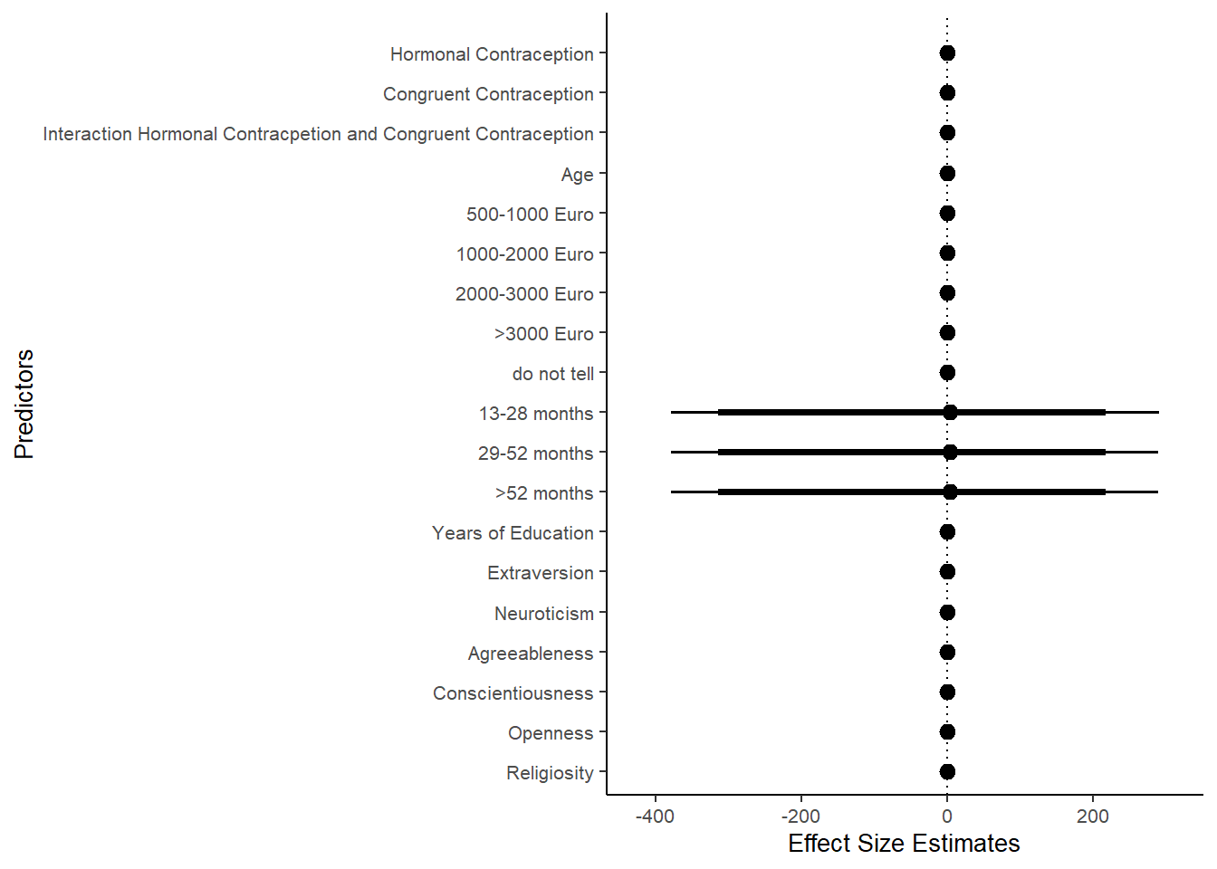
Masturbation Frequency
Model
m_congruency_masfreq_controlled = brm(diary_masturbation_sum ~
                        offset(log(number_of_days)) +
                        contraception_hormonal * congruent_contraception +
                        age + net_income + relationship_duration_factor +
                              education_years +
                              bfi_extra + bfi_neuro + bfi_agree + bfi_consc + bfi_open +
                              religiosity,
                data = data, family = poisson(),
                file = "m_congruency_masfreq_controlled")
Summary
##  Family: poisson
##   Links: mu = log
## Formula: diary_masturbation_sum ~ offset(log(number_of_days)) + contraception_hormonal * congruent_contraception + age + net_income + relationship_duration_factor + education_years + bfi_extra + bfi_neuro + bfi_agree + bfi_consc + bfi_open + religiosity
##    Data: data (Number of observations: 622)
##   Draws: 4 chains, each with iter = 2000; warmup = 1000; thin = 1;
##          total post-warmup draws = 4000
##
## Population-Level Effects:
##                                                        Estimate Est.Error l-90% CI u-90% CI Rhat Bulk_ESS
## Intercept                                                 -1.74      0.23    -2.12    -1.36 1.00     4718
## contraception_hormonalyes                                 -0.38      0.06    -0.47    -0.28 1.00     3090
## congruent_contraception1                                   0.04      0.05    -0.04     0.12 1.00     3121
## age                                                       -0.01      0.00    -0.02    -0.00 1.00     4213
## net_incomeeuro_500_1000                                    0.18      0.04     0.11     0.25 1.00     3789
## net_incomeeuro_1000_2000                                   0.21      0.06     0.12     0.31 1.00     3356
## net_incomeeuro_2000_3000                                   0.07      0.08    -0.07     0.20 1.00     3447
## net_incomeeuro_gt_3000                                    -0.13      0.15    -0.37     0.11 1.00     4879
## net_incomedont_tell                                       -0.18      0.12    -0.37     0.01 1.00     4786
## relationship_duration_factorPartnered_upto28months        -0.03      0.04    -0.11     0.04 1.00     3792
## relationship_duration_factorPartnered_upto52months        -0.07      0.05    -0.15     0.01 1.00     3586
## relationship_duration_factorPartnered_morethan52months    -0.20      0.05    -0.28    -0.12 1.00     3790
## education_years                                            0.00      0.00    -0.00     0.01 1.00     5824
## bfi_extra                                                 -0.02      0.02    -0.06     0.02 1.00     4565
## bfi_neuro                                                  0.00      0.02    -0.04     0.04 1.00     4670
## bfi_agree                                                  0.01      0.03    -0.04     0.06 1.00     4377
## bfi_consc                                                 -0.22      0.03    -0.26    -0.18 1.00     5098
## bfi_open                                                   0.20      0.03     0.15     0.25 1.00     5236
## religiosity                                               -0.06      0.01    -0.08    -0.04 1.00     4483
## contraception_hormonalyes:congruent_contraception1         0.10      0.07    -0.02     0.22 1.00     2862
##                                                        Tail_ESS
## Intercept                                                  3203
## contraception_hormonalyes                                  2694
## congruent_contraception1                                   2405
## age                                                        3421
## net_incomeeuro_500_1000                                    3027
## net_incomeeuro_1000_2000                                   2833
## net_incomeeuro_2000_3000                                   3065
## net_incomeeuro_gt_3000                                     3343
## net_incomedont_tell                                        3204
## relationship_duration_factorPartnered_upto28months         3010
## relationship_duration_factorPartnered_upto52months         3355
## relationship_duration_factorPartnered_morethan52months     3275
## education_years                                            3022
## bfi_extra                                                  2643
## bfi_neuro                                                  2568
## bfi_agree                                                  3140
## bfi_consc                                                  3185
## bfi_open                                                   3192
## religiosity                                                3143
## contraception_hormonalyes:congruent_contraception1         2727
##
## Draws were sampled using sampling(NUTS). For each parameter, Bulk_ESS
## and Tail_ESS are effective sample size measures, and Rhat is the potential
## scale reduction factor on split chains (at convergence, Rhat = 1).
Comparison with ROPE
plot(equivalence_test(m_congruency_masfreq_controlled, range = c(-0.05, 0.05), ci = 0.90,
                      parameters = "contraception"))
## Possible multicollinearity between b_contraception_hormonalyes:congruent_contraception1 and b_contraception_hormonalyes (r = 0.8). This might lead to inappropriate results. See 'Details' in '?equivalence_test'.## Picking joint bandwidth of 0.00819## Warning: Removed 1197 rows containing non-finite values (stat_density_ridges).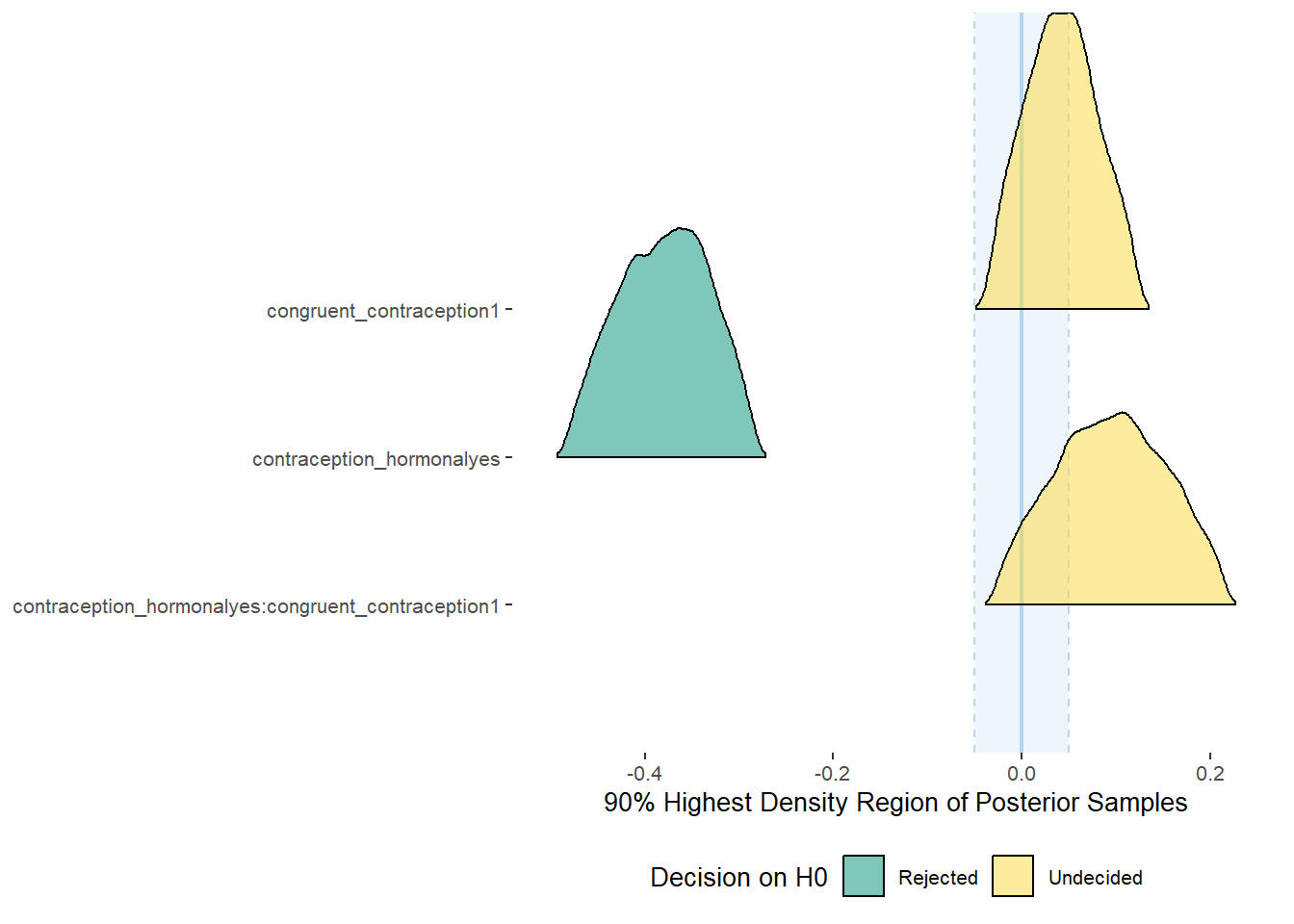
equivalence_test(m_congruency_masfreq_controlled, range = c(-0.05, 0.05), ci = 0.90,
                      parameters = "contraception")
## Possible multicollinearity between b_contraception_hormonalyes:congruent_contraception1 and b_contraception_hormonalyes (r = 0.8). This might lead to inappropriate results. See 'Details' in '?equivalence_test'.## # A tibble: 3 x 10
## Parameter CI ROPE_low ROPE_high ROPE_Percentage ROPE_Equivalence HDI_low HDI_high Effects Component
## <chr> <dbl> <dbl> <dbl> <dbl> <chr> <dbl> <dbl> <chr> <chr>
## 1 b_contraceptio~ 0.9 -0.05 0.05 0 Rejected -0.479 -0.286 fixed conditio~
## 2 b_congruent_co~ 0.9 -0.05 0.05 0.573 Undecided -0.0332 0.121 fixed conditio~
## 3 b_contraceptio~ 0.9 -0.05 0.05 0.244 Undecided -0.0244 0.213 fixed conditio~Plots
conditional_effects(m_congruency_masfreq_controlled,
                    effects = "contraception_hormonal:congruent_contraception",
                    conditions = data.frame(number_of_days = 1))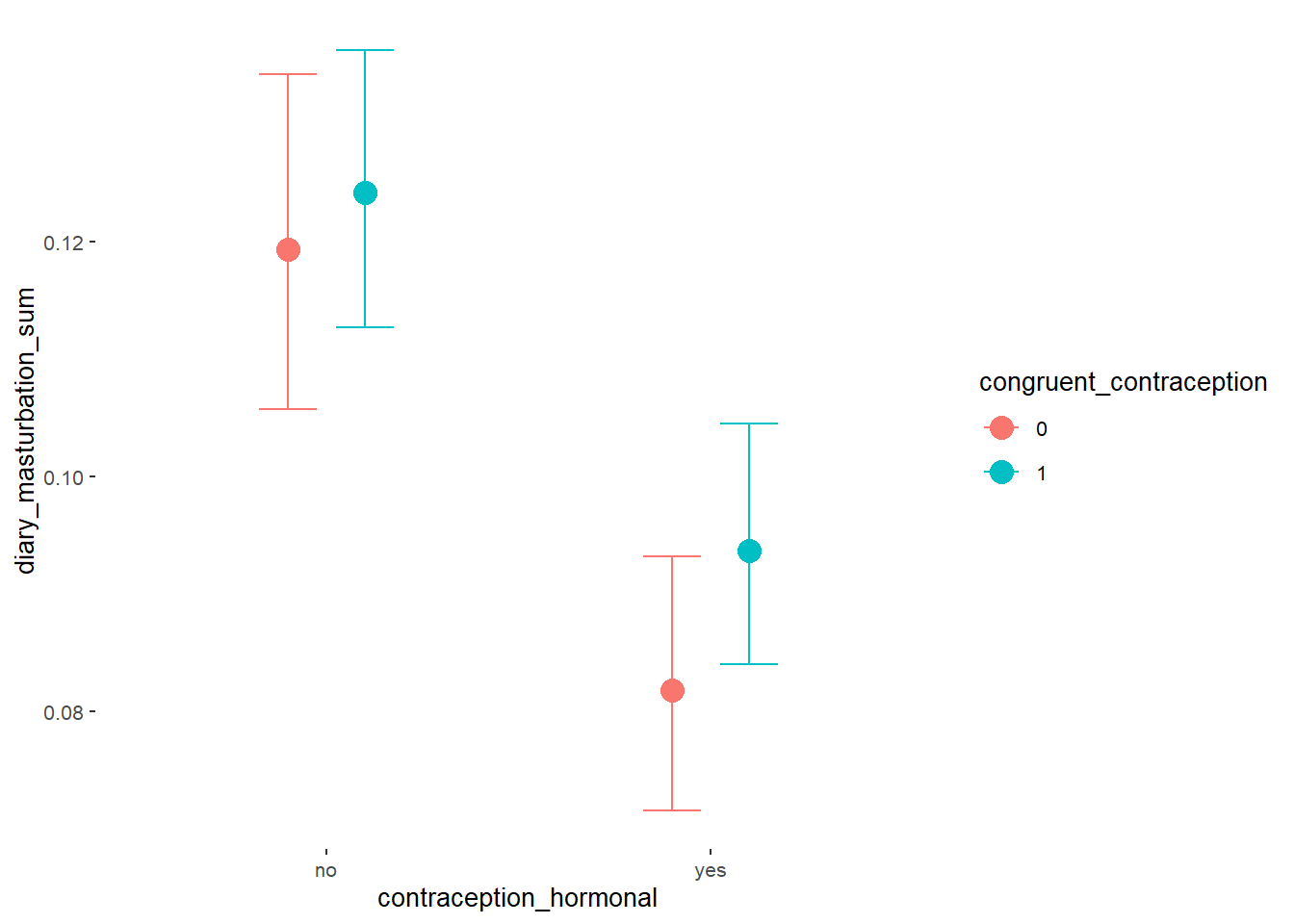
Forest Plot for Effect Sizes
m_congruency_masfreq_controlled %>%

  spread_draws(b_contraception_hormonalyes, b_congruent_contraception1,
               `b_contraception_hormonalyes:congruent_contraception1`,
               b_age,
               b_net_incomeeuro_500_1000, b_net_incomeeuro_1000_2000,
               b_net_incomeeuro_2000_3000, b_net_incomeeuro_gt_3000, b_net_incomedont_tell,
               b_relationship_duration_factorPartnered_upto28months,
               b_relationship_duration_factorPartnered_upto52months,
               b_relationship_duration_factorPartnered_morethan52months,
               b_education_years,
               b_bfi_extra, b_bfi_neuro, b_bfi_agree, b_bfi_consc, b_bfi_open,
               b_religiosity) %>%
  pivot_longer(cols = c(b_contraception_hormonalyes, b_congruent_contraception1,
               `b_contraception_hormonalyes:congruent_contraception1`,
                        b_age,
               b_net_incomeeuro_500_1000, b_net_incomeeuro_1000_2000,
               b_net_incomeeuro_2000_3000, b_net_incomeeuro_gt_3000, b_net_incomedont_tell,
               b_relationship_duration_factorPartnered_upto28months,
               b_relationship_duration_factorPartnered_upto52months,
               b_relationship_duration_factorPartnered_morethan52months,
               b_education_years,
               b_bfi_extra, b_bfi_neuro, b_bfi_agree, b_bfi_consc, b_bfi_open,
               b_religiosity),
               names_to = "condition",
               values_to = "r_condition") %>%
  mutate(condition_mean = r_condition,
         group = ifelse(condition %contains% "b_relationship_duration_factor",
                        "Relationship Duration",
                        ifelse(condition %contains% "b_net_income",
                               "Income",
                               NA)),
         group = ifelse(condition %contains% "ontraception",
                        "Contraception", group),
         condition = ifelse(condition == "b_contraception_hormonalyes",
                        "Hormonal Contraception",
                     ifelse(condition == "b_congruent_contraception1",
                            "Congruent Contraception",
                     ifelse(condition == "b_contraception_hormonalyes:congruent_contraception1",
                            "Interaction Hormonal Contracpetion and Congruent Contraception",
                            condition))),
         condition = ifelse(condition == "b_age", "Age",
                ifelse(condition == "b_net_incomeeuro_500_1000", "500-1000 Euro",
                ifelse(condition == "b_net_incomeeuro_1000_2000", "1000-2000 Euro",
                ifelse(condition == "b_net_incomeeuro_2000_3000", "2000-3000 Euro",
                ifelse(condition == "b_net_incomeeuro_gt_3000", ">3000 Euro",
                ifelse(condition == "b_net_incomedont_tell", "do not tell",
                ifelse(condition == "b_relationship_duration_factorPartnered_upto28months",
                       "13-28 months",
                ifelse(condition == "b_relationship_duration_factorPartnered_upto52months",
                       "29-52 months",
                ifelse(condition == "b_relationship_duration_factorPartnered_morethan52months",
                       ">52 months",
                ifelse(condition == "b_education_years", "Years of Education",
                ifelse(condition == "b_bfi_extra", "Extraversion",
                ifelse(condition == "b_bfi_neuro", "Neuroticism",
                ifelse(condition == "b_bfi_agree", "Agreeableness",
                ifelse(condition == "b_bfi_consc", "Conscientiousness",
                ifelse(condition == "b_bfi_open", "Openness",
                ifelse(condition == "b_religiosity", "Religiosity",
                       condition)))))))))))))))),
         group = ifelse(is.na(group), condition, group),
         condition = factor(condition, levels = rev(c("Hormonal Contraception",
                                        "Congruent Contraception",
                                        "Interaction Hormonal Contracpetion and Congruent Contraception",
                                        "Age",
                                        "500-1000 Euro", "1000-2000 Euro",
                                        "2000-3000 Euro", ">3000 Euro", "do not tell",
                                        "13-28 months", "29-52 months",
                                        ">52 months",
                                        "Years of Education",
                                        "Extraversion", "Neuroticism", "Agreeableness",
                                         "Conscientiousness","Openness","Religiosity"))),
         group = factor(group, levels = c("Contraception", "Age", "Income",
                                          "Relationship Duration","Years of Education",
                                          "Extraversion", "Neuroticism", "Agreeableness",
                                         "Conscientiousness","Openness","Religiosity"))) %>%
  ggplot(aes(y = condition,
             x = condition_mean,
             fill = stat(abs(x) < 0.05))) +
  stat_halfeye() +
  geom_vline(xintercept = c(-0.05, 0.05), linetype = "dotted") +
  apatheme +
  theme(legend.position = "none") +
  scale_fill_manual(values = c("gray80", "skyblue")) +
  labs(x = "Effect Size Estimates", y = "Predictors")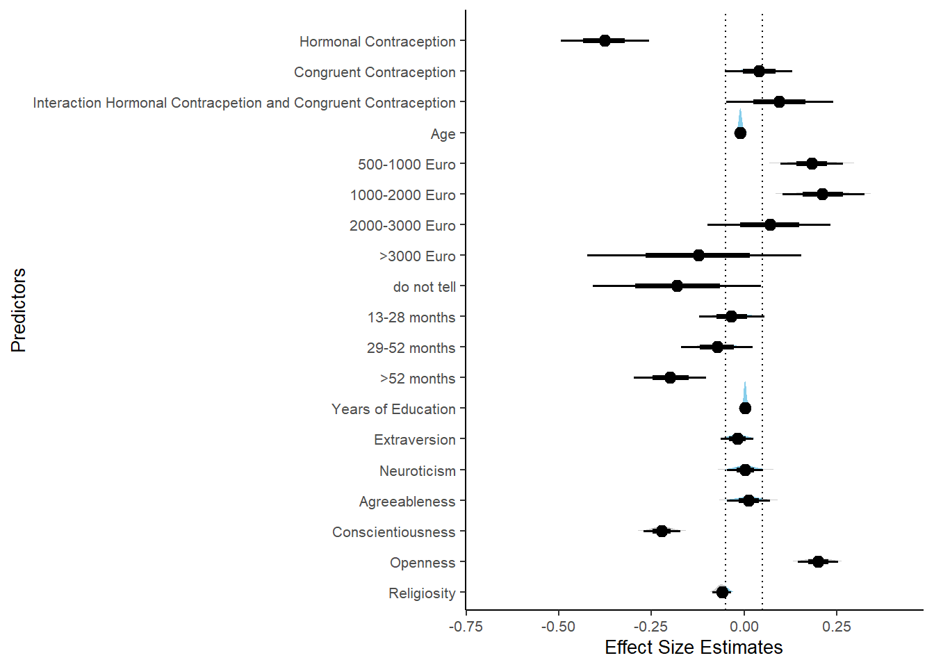
Model Comparison
Attractiveness of partner
LooIC first model: 1726.1
LooIC second model: 1726.72
Model Comparisons: The difference between models is -0.31 compared to a standard error of 1.86
## Output of model 'm_hc_atrr':
##
## Computed from 4000 by 774 log-likelihood matrix
##
##          Estimate   SE
## elpd_loo   -863.0 23.1
## p_loo         3.3  0.4
## looic      1726.1 46.2
## ------
## Monte Carlo SE of elpd_loo is 0.0.
##
## All Pareto k estimates are good (k < 0.5).
## See help('pareto-k-diagnostic') for details.
##
## Output of model 'm_congruency_atrr':
##
## Computed from 4000 by 774 log-likelihood matrix
##
##          Estimate   SE
## elpd_loo   -863.4 23.2
## p_loo         5.3  0.5
## looic      1726.7 46.5
## ------
## Monte Carlo SE of elpd_loo is 0.0.
##
## All Pareto k estimates are good (k < 0.5).
## See help('pareto-k-diagnostic') for details.
##
## Model comparisons:
##                   elpd_diff se_diff
## m_hc_atrr          0.0       0.0
## m_congruency_atrr -0.3       1.9
Relationship satisfaction
LooIC first model: 872.85
LooIC second model: 870.03
Model Comparisons: The difference between models is -1.41 compared to a standard error of 2.66
## Output of model 'm_hc_relsat':
##
## Computed from 4000 by 774 log-likelihood matrix
##
##          Estimate   SE
## elpd_loo   -436.4 26.6
## p_loo         3.9  0.5
## looic       872.9 53.2
## ------
## Monte Carlo SE of elpd_loo is 0.0.
##
## All Pareto k estimates are good (k < 0.5).
## See help('pareto-k-diagnostic') for details.
##
## Output of model 'm_congruency_relsat':
##
## Computed from 4000 by 774 log-likelihood matrix
##
##          Estimate   SE
## elpd_loo   -435.0 26.3
## p_loo         5.8  0.6
## looic       870.0 52.5
## ------
## Monte Carlo SE of elpd_loo is 0.0.
##
## All Pareto k estimates are good (k < 0.5).
## See help('pareto-k-diagnostic') for details.
##
## Model comparisons:
##                     elpd_diff se_diff
## m_congruency_relsat  0.0       0.0
## m_hc_relsat         -1.4       2.7
Sexual Satisfaction
m_hc_sexsat$data$satisfaction_sexual_intercourse =
  as.numeric(m_hc_sexsat$data$satisfaction_sexual_intercourse)
m_congruency_sexsat$data$satisfaction_sexual_intercourse =
  as.numeric(m_congruency_sexsat$data$satisfaction_sexual_intercourse)

compare_models = loo(m_hc_sexsat, m_congruency_sexsat)
LooIC first model: 2276.46
LooIC second model: 2277.93
Model Comparisons: The difference between models is -0.74 compared to a standard error of 1.61
## Output of model 'm_hc_sexsat':
##
## Computed from 4000 by 774 log-likelihood matrix
##
##          Estimate   SE
## elpd_loo  -1138.2 21.0
## p_loo         3.2  0.3
## looic      2276.5 42.0
## ------
## Monte Carlo SE of elpd_loo is 0.0.
##
## All Pareto k estimates are good (k < 0.5).
## See help('pareto-k-diagnostic') for details.
##
## Output of model 'm_congruency_sexsat':
##
## Computed from 4000 by 774 log-likelihood matrix
##
##          Estimate   SE
## elpd_loo  -1139.0 21.0
## p_loo         5.1  0.4
## looic      2277.9 42.1
## ------
## Monte Carlo SE of elpd_loo is 0.0.
##
## All Pareto k estimates are good (k < 0.5).
## See help('pareto-k-diagnostic') for details.
##
## Model comparisons:
##                     elpd_diff se_diff
## m_hc_sexsat          0.0       0.0
## m_congruency_sexsat -0.7       1.6
LS0tDQp0aXRsZTogIkFuYWx5c2VzIEVmZmVjdHMgb2YgQ29udHJhY2VwdGlvbiINCm91dHB1dDoNCiAgaHRtbF9kb2N1bWVudDoNCiAgICB0b2M6IHRydWUNCiAgICB0b2NfZGVwdGg6IDQNCiAgICB0b2NfZmxvYXQ6IHRydWUNCiAgICBjb2RlX2ZvbGRpbmc6ICdoaWRlJw0KICAgIHNlbGZfY29udGFpbmVkOiBmYWxzZQ0KZWRpdG9yX29wdGlvbnM6IA0KICBjaHVua19vdXRwdXRfdHlwZTogY29uc29sZQ0KLS0tDQogIA0KICANCiMjIERhdGEgDQpgYGB7ciByZXN1bHRzPSdoaWRlJyxtZXNzYWdlPUYsd2FybmluZz1GfQ0Kc291cmNlKCIwX2hlbHBlcnMuUiIpDQoNCmxvYWQoImRhdGEvY2xlYW5lZF9zZWxlY3RlZF93cmFuZ2xlZC5yZGF0YSIpDQpgYGANCg0KDQojIyBFZmZlY3RzIG9mIEhvcm1vbmFsIENvbnRyYWNlcHRpdmVzIHsudGFic2V0fQ0KIyMjIEF0dHJhY3RpdmVuZXNzIG9mIFBhcnRuZXIgey50YWJzZXR9DQojIyMjIE1vZGVsDQpgYGB7cn0NCm1faGNfYXRyciA9IGJybShhdHRyYWN0aXZlbmVzc19wYXJ0bmVyIH4gY29udHJhY2VwdGlvbl9ob3Jtb25hbCwNCiAgICAgICAgICAgICAgICBkYXRhID0gZGF0YSwgZmFtaWx5ID0gZ2F1c3NpYW4oKSwNCiAgICAgICAgICAgICAgICBmaWxlID0gIm1faGNfYXRyciIpDQpgYGANCg0KIyMjIyBTdW1tYXJ5DQpgYGB7cn0NCnN1bW1hcnkobV9oY19hdHJyLCBpbnRlcnZhbHMgPSBULCBwcm9iID0gMC45MCkNCmBgYA0KDQojIyMjIENvbXBhcmlzb24gd2l0aCBST1BFDQpgYGB7cn0NCnBsb3QoZXF1aXZhbGVuY2VfdGVzdChtX2hjX2F0cnIsIHJhbmdlID0gYygtMC4wNywgMC4wNyksIGNpID0gMC45MCwNCiAgICAgICAgICAgICAgICAgICAgICBwYXJhbWV0ZXJzID0gImNvbnRyYWNlcHRpb24iKSkNCmVxdWl2YWxlbmNlX3Rlc3QobV9oY19hdHJyLCByYW5nZSA9IGMoLTAuMDcsIDAuMDcpLCBjaSA9IDAuOTAsDQogICAgICAgICAgICAgICAgICAgICAgcGFyYW1ldGVycyA9ICJjb250cmFjZXB0aW9uIikNCmBgYA0KDQojIyMjIFBsb3RzDQpgYGB7ciB3YXJuaW5nID0gRkFMU0V9DQpjb25kaXRpb25hbF9lZmZlY3RzKG1faGNfYXRyciwgYXNrID0gRkFMU0UpDQpgYGANCg0KIyMjIyBGb3Jlc3QgUGxvdCBmb3IgRWZmZWN0IFNpemVzIHsuYWN0aXZlfQ0KYGBge3J9DQptX2hjX2F0cnIgJT4lDQogIHNwcmVhZF9kcmF3cyhiX2NvbnRyYWNlcHRpb25faG9ybW9uYWx5ZXMpICU+JQ0KICBwaXZvdF9sb25nZXIoY29scyA9IGMoYl9jb250cmFjZXB0aW9uX2hvcm1vbmFseWVzKSwNCiAgICAgICAgICAgICAgIG5hbWVzX3RvID0gImNvbmRpdGlvbiIsDQogICAgICAgICAgICAgICB2YWx1ZXNfdG8gPSAicl9jb25kaXRpb24iKSAlPiUNCiAgbXV0YXRlKGNvbmRpdGlvbl9tZWFuID0gcl9jb25kaXRpb24sDQogICAgICAgICBncm91cCA9IGlmZWxzZShjb25kaXRpb24gJWNvbnRhaW5zJSAiYl9jb250cmFjZXB0aW9uX2hvcm1vbmFseWVzIiwNCiAgICAgICAgICAgICAgICAgICAgICAgICJDb250cmFjZXB0aW9uIiwgTkEpLA0KICAgICAgICAgY29uZGl0aW9uID0gaWZlbHNlKGNvbmRpdGlvbiAlY29udGFpbnMlICJiX2NvbnRyYWNlcHRpb25faG9ybW9uYWx5ZXMiLA0KICAgICAgICAgICAgICAgICAgICAgICAgIkhvcm1vbmFsIENvbnRyYWNlcHRpb24iLCBOQSkpICU+JQ0KICBnZ3Bsb3QoYWVzKHkgPSBjb25kaXRpb24sDQogICAgICAgICAgICAgeCA9IGNvbmRpdGlvbl9tZWFuLA0KICAgICAgICAgICAgIGZpbGwgPSBzdGF0KGFicyh4KSA8IDAuMDcpKSkgKw0KICBzdGF0X2hhbGZleWUoKSArDQogIGdlb21fdmxpbmUoeGludGVyY2VwdCA9IGMoLTAuMDcsIDAuMDcpLCBsaW5ldHlwZSA9ICJkb3R0ZWQiKSArDQogIGFwYXRoZW1lICsNCiAgdGhlbWUobGVnZW5kLnBvc2l0aW9uID0gIm5vbmUiKSArDQogIHNjYWxlX2ZpbGxfbWFudWFsKHZhbHVlcyA9IGMoImdyYXk4MCIsICJza3libHVlIikpICsNCiAgbGFicyh4ID0gIkVmZmVjdCBTaXplIEVzdGltYXRlcyIsIHkgPSAiUHJlZGljdG9ycyIpICsNCiAgeGxpbSAoLTAuNiwgMC42KQ0KYGBgDQoNCiMjIyBSZWxhdGlvbnNoaXAgU2F0aXNmYWN0aW9uIHsudGFic2V0fQ0KIyMjIyBNb2RlbA0KYGBge3J9DQptX2hjX3JlbHNhdCA9IGJybShyZWxhdGlvbnNoaXBfc2F0aXNmYWN0aW9uIH4gY29udHJhY2VwdGlvbl9ob3Jtb25hbCwNCiAgICAgICAgICAgICAgICBkYXRhID0gZGF0YSwgZmFtaWx5ID0gZ2F1c3NpYW4oKSwNCiAgICAgICAgICAgICAgICBmaWxlID0gIm1faGNfcmVsc2F0IikNCmBgYA0KDQojIyMjIFN1bW1hcnkNCmBgYHtyfQ0Kc3VtbWFyeShtX2hjX3JlbHNhdCwgaW50ZXJ2YWxzID0gVCwgcHJvYiA9IDAuOTApDQpgYGANCg0KIyMjIyBDb21wYXJpc29uIHdpdGggUk9QRQ0KYGBge3J9DQpwbG90KGVxdWl2YWxlbmNlX3Rlc3QobV9oY19yZWxzYXQsIHJhbmdlID0gYygtMC4wNCwgMC4wNCksIGNpID0gMC45MCwNCiAgICAgICAgICAgICAgICAgICAgICBwYXJhbWV0ZXJzID0gImNvbnRyYWNlcHRpb24iKSkNCmVxdWl2YWxlbmNlX3Rlc3QobV9oY19yZWxzYXQsIHJhbmdlID0gYygtMC4wNCwgMC4wNCksIGNpID0gMC45MCwNCiAgICAgICAgICAgICAgICAgICAgICBwYXJhbWV0ZXJzID0gImNvbnRyYWNlcHRpb24iKQ0KYGBgDQoNCiMjIyMgUGxvdHMNCmBgYHtyIHdhcm5pbmcgPSBGQUxTRX0NCmNvbmRpdGlvbmFsX2VmZmVjdHMobV9oY19yZWxzYXQsIGFzayA9IEZBTFNFKQ0KYGBgDQoNCiMjIyMgRm9yZXN0IFBsb3QgZm9yIEVmZmVjdCBTaXplcyB7LmFjdGl2ZX0NCmBgYHtyfQ0KbV9oY19yZWxzYXQgJT4lDQogIHNwcmVhZF9kcmF3cyhiX2NvbnRyYWNlcHRpb25faG9ybW9uYWx5ZXMpICU+JQ0KICBwaXZvdF9sb25nZXIoY29scyA9IGMoYl9jb250cmFjZXB0aW9uX2hvcm1vbmFseWVzKSwNCiAgICAgICAgICAgICAgIG5hbWVzX3RvID0gImNvbmRpdGlvbiIsDQogICAgICAgICAgICAgICB2YWx1ZXNfdG8gPSAicl9jb25kaXRpb24iKSAlPiUNCiAgbXV0YXRlKGNvbmRpdGlvbl9tZWFuID0gcl9jb25kaXRpb24sDQogICAgICAgICBncm91cCA9IGlmZWxzZShjb25kaXRpb24gJWNvbnRhaW5zJSAiYl9jb250cmFjZXB0aW9uX2hvcm1vbmFseWVzIiwNCiAgICAgICAgICAgICAgICAgICAgICAgICJDb250cmFjZXB0aW9uIiwgTkEpLA0KICAgICAgICAgY29uZGl0aW9uID0gaWZlbHNlKGNvbmRpdGlvbiAlY29udGFpbnMlICJiX2NvbnRyYWNlcHRpb25faG9ybW9uYWx5ZXMiLA0KICAgICAgICAgICAgICAgICAgICAgICAgIkhvcm1vbmFsIENvbnRyYWNlcHRpb24iLCBOQSkpICU+JQ0KICBnZ3Bsb3QoYWVzKHkgPSBjb25kaXRpb24sDQogICAgICAgICAgICAgeCA9IGNvbmRpdGlvbl9tZWFuLA0KICAgICAgICAgICAgIGZpbGwgPSBzdGF0KGFicyh4KSA8IDAuMDQpKSkgKw0KICBzdGF0X2hhbGZleWUoKSArDQogIGdlb21fdmxpbmUoeGludGVyY2VwdCA9IGMoLTAuMDQsIDAuMDQpLCBsaW5ldHlwZSA9ICJkb3R0ZWQiKSArDQogIGFwYXRoZW1lICsNCiAgdGhlbWUobGVnZW5kLnBvc2l0aW9uID0gIm5vbmUiKSArDQogIHNjYWxlX2ZpbGxfbWFudWFsKHZhbHVlcyA9IGMoImdyYXk4MCIsICJza3libHVlIikpICsNCiAgbGFicyh4ID0gIkVmZmVjdCBTaXplIEVzdGltYXRlcyIsIHkgPSAiUHJlZGljdG9ycyIpICsNCiAgeGxpbSAoLTAuNiwgMC42KQ0KYGBgDQoNCg0KIyMjIFNleHVhbCBTYXRpc2ZhY3Rpb24gey50YWJzZXR9DQojIyMjIE1vZGVsDQpgYGB7cn0NCm1faGNfc2V4c2F0ID0gYnJtKHNhdGlzZmFjdGlvbl9zZXh1YWxfaW50ZXJjb3Vyc2UgfiBjb250cmFjZXB0aW9uX2hvcm1vbmFsLA0KICAgICAgICAgICAgICAgIGRhdGEgPSBkYXRhLCBmYW1pbHkgPSBnYXVzc2lhbigpLA0KICAgICAgICAgICAgICAgIGZpbGUgPSAibV9oY19zZXhzYXQiKQ0KYGBgDQoNCiMjIyMgU3VtbWFyeQ0KYGBge3J9DQpzdW1tYXJ5KG1faGNfc2V4c2F0LCBpbnRlcnZhbHMgPSBULCBwcm9iID0gMC45MCkNCmBgYA0KDQojIyMjIENvbXBhcmlzb24gd2l0aCBST1BFDQpgYGB7cn0NCnBsb3QoZXF1aXZhbGVuY2VfdGVzdChtX2hjX3NleHNhdCwgcmFuZ2UgPSBjKC0wLjExLCAwLjExKSwgY2kgPSAwLjkwLA0KICAgICAgICAgICAgICAgICAgICAgIHBhcmFtZXRlcnMgPSAiY29udHJhY2VwdGlvbiIpKQ0KZXF1aXZhbGVuY2VfdGVzdChtX2hjX3NleHNhdCwgcmFuZ2UgPSBjKC0wLjExLCAwLjExKSwgY2kgPSAwLjkwLA0KICAgICAgICAgICAgICAgICAgICAgIHBhcmFtZXRlcnMgPSAiY29udHJhY2VwdGlvbiIpDQpgYGANCg0KIyMjIyBQbG90cw0KYGBge3Igd2FybmluZyA9IEZBTFNFfQ0KY29uZGl0aW9uYWxfZWZmZWN0cyhtX2hjX3NleHNhdCwgYXNrID0gRkFMU0UpDQpgYGANCg0KIyMjIyBGb3Jlc3QgUGxvdCBmb3IgRWZmZWN0IFNpemVzIHsuYWN0aXZlfQ0KYGBge3J9DQptX2hjX3NleHNhdCAlPiUNCiAgc3ByZWFkX2RyYXdzKGJfY29udHJhY2VwdGlvbl9ob3Jtb25hbHllcykgJT4lDQogIHBpdm90X2xvbmdlcihjb2xzID0gYyhiX2NvbnRyYWNlcHRpb25faG9ybW9uYWx5ZXMpLA0KICAgICAgICAgICAgICAgbmFtZXNfdG8gPSAiY29uZGl0aW9uIiwNCiAgICAgICAgICAgICAgIHZhbHVlc190byA9ICJyX2NvbmRpdGlvbiIpICU+JQ0KICBtdXRhdGUoY29uZGl0aW9uX21lYW4gPSByX2NvbmRpdGlvbiwNCiAgICAgICAgIGdyb3VwID0gaWZlbHNlKGNvbmRpdGlvbiAlY29udGFpbnMlICJiX2NvbnRyYWNlcHRpb25faG9ybW9uYWx5ZXMiLA0KICAgICAgICAgICAgICAgICAgICAgICAgIkNvbnRyYWNlcHRpb24iLCBOQSksDQogICAgICAgICBjb25kaXRpb24gPSBpZmVsc2UoY29uZGl0aW9uICVjb250YWlucyUgImJfY29udHJhY2VwdGlvbl9ob3Jtb25hbHllcyIsDQogICAgICAgICAgICAgICAgICAgICAgICAiSG9ybW9uYWwgQ29udHJhY2VwdGlvbiIsIE5BKSkgJT4lDQogIGdncGxvdChhZXMoeSA9IGNvbmRpdGlvbiwNCiAgICAgICAgICAgICB4ID0gY29uZGl0aW9uX21lYW4sDQogICAgICAgICAgICAgZmlsbCA9IHN0YXQoYWJzKHgpIDwgMC4xMSkpKSArDQogIHN0YXRfaGFsZmV5ZSgpICsNCiAgZ2VvbV92bGluZSh4aW50ZXJjZXB0ID0gYygtMC4xMSwgMC4xMSksIGxpbmV0eXBlID0gImRvdHRlZCIpICsNCiAgYXBhdGhlbWUgKw0KICB0aGVtZShsZWdlbmQucG9zaXRpb24gPSAibm9uZSIpICsNCiAgc2NhbGVfZmlsbF9tYW51YWwodmFsdWVzID0gYygiZ3JheTgwIiwgInNreWJsdWUiKSkgKw0KICBsYWJzKHggPSAiRWZmZWN0IFNpemUgRXN0aW1hdGVzIiwgeSA9ICJQcmVkaWN0b3JzIikgKw0KICB4bGltICgtMC42LCAwLjYpDQpgYGANCg0KIyMjIExpYmlkbyB7LnRhYnNldH0NCg0KIyMjIyBNb2RlbA0KYGBge3J9DQptX2hjX2xpYmlkbyA9IGJybShkaWFyeV9saWJpZG9fbWVhbiB+IGNvbnRyYWNlcHRpb25faG9ybW9uYWwsDQogICAgICAgICAgICAgICAgZGF0YSA9IGRhdGEsIGZhbWlseSA9IGdhdXNzaWFuKCksDQogICAgICAgICAgICAgICAgZmlsZSA9ICJtX2hjX2xpYmlkbyIpDQpgYGANCg0KIyMjIyBTdW1tYXJ5DQpgYGB7cn0NCnN1bW1hcnkobV9oY19saWJpZG8sIGludGVydmFscyA9IFQsIHByb2IgPSAwLjkwKQ0KYGBgDQoNCiMjIyMgQ29tcGFyaXNvbiB3aXRoIFJPUEUNCmBgYHtyfQ0KcGxvdChlcXVpdmFsZW5jZV90ZXN0KG1faGNfbGliaWRvLCByYW5nZSA9IGMoLTAuMDYsIDAuMDYpLCBjaSA9IDAuOTAsDQogICAgICAgICAgICAgICAgICAgICAgcGFyYW1ldGVycyA9ICJjb250cmFjZXB0aW9uIikpDQplcXVpdmFsZW5jZV90ZXN0KG1faGNfbGliaWRvLCByYW5nZSA9IGMoLTAuMDYsIDAuMDYpLCBjaSA9IDAuOTAsDQogICAgICAgICAgICAgICAgICAgICAgcGFyYW1ldGVycyA9ICJjb250cmFjZXB0aW9uIikNCmBgYA0KDQojIyMjIFBsb3RzDQpgYGB7ciB3YXJuaW5nID0gRkFMU0V9DQpjb25kaXRpb25hbF9lZmZlY3RzKG1faGNfbGliaWRvLCBhc2sgPSBGQUxTRSkNCmBgYA0KDQojIyMjIEZvcmVzdCBQbG90IGZvciBFZmZlY3QgU2l6ZXMgey5hY3RpdmV9DQpgYGB7cn0NCm1faGNfbGliaWRvICU+JQ0KICBzcHJlYWRfZHJhd3MoYl9jb250cmFjZXB0aW9uX2hvcm1vbmFseWVzKSAlPiUNCiAgcGl2b3RfbG9uZ2VyKGNvbHMgPSBjKGJfY29udHJhY2VwdGlvbl9ob3Jtb25hbHllcyksDQogICAgICAgICAgICAgICBuYW1lc190byA9ICJjb25kaXRpb24iLA0KICAgICAgICAgICAgICAgdmFsdWVzX3RvID0gInJfY29uZGl0aW9uIikgJT4lDQogIG11dGF0ZShjb25kaXRpb25fbWVhbiA9IHJfY29uZGl0aW9uLA0KICAgICAgICAgZ3JvdXAgPSBpZmVsc2UoY29uZGl0aW9uICVjb250YWlucyUgImJfY29udHJhY2VwdGlvbl9ob3Jtb25hbHllcyIsDQogICAgICAgICAgICAgICAgICAgICAgICAiQ29udHJhY2VwdGlvbiIsIE5BKSwNCiAgICAgICAgIGNvbmRpdGlvbiA9IGlmZWxzZShjb25kaXRpb24gJWNvbnRhaW5zJSAiYl9jb250cmFjZXB0aW9uX2hvcm1vbmFseWVzIiwNCiAgICAgICAgICAgICAgICAgICAgICAgICJIb3Jtb25hbCBDb250cmFjZXB0aW9uIiwgTkEpKSAlPiUNCiAgZ2dwbG90KGFlcyh5ID0gY29uZGl0aW9uLA0KICAgICAgICAgICAgIHggPSBjb25kaXRpb25fbWVhbiwNCiAgICAgICAgICAgICBmaWxsID0gc3RhdChhYnMoeCkgPCAwLjA2KSkpICsNCiAgc3RhdF9oYWxmZXllKCkgKw0KICBnZW9tX3ZsaW5lKHhpbnRlcmNlcHQgPSBjKC0wLjA2LCAwLjA2KSwgbGluZXR5cGUgPSAiZG90dGVkIikgKw0KICBhcGF0aGVtZSArDQogIHRoZW1lKGxlZ2VuZC5wb3NpdGlvbiA9ICJub25lIikgKw0KICBzY2FsZV9maWxsX21hbnVhbCh2YWx1ZXMgPSBjKCJncmF5ODAiLCAic2t5Ymx1ZSIpKSArDQogIGxhYnMoeCA9ICJFZmZlY3QgU2l6ZSBFc3RpbWF0ZXMiLCB5ID0gIlByZWRpY3RvcnMiKSArDQogIHhsaW0gKC0wLjYsIDAuNikNCmBgYA0KDQoNCiMjIyBTZXh1YWwgRnJlcXVlbmN5IChQZW5ldHJhdGl2ZSBJbnRlcmNvdXJzZSkgey50YWJzZXR9DQojIyMjIE1vZGVsDQpgYGB7cn0NCm1faGNfc2V4ZnJlcXBlbiA9IGJybShkaWFyeV9zZXhfYWN0aXZlX3NleF9zdW0gfg0KICAgICAgICAgICAgICAgICAgICAgICAgb2Zmc2V0KGxvZyhudW1iZXJfb2ZfZGF5cykpICsNCiAgICAgICAgICAgICAgICAgICAgICAgIGNvbnRyYWNlcHRpb25faG9ybW9uYWwsDQogICAgICAgICAgICAgICAgZGF0YSA9IGRhdGEsIGZhbWlseSA9IHBvaXNzb24oKSwNCiAgICAgICAgICAgICAgICBmaWxlID0gIm1faGNfc2V4ZnJlcXBlbiIpDQpgYGANCg0KIyMjIyBTdW1tYXJ5DQpgYGB7cn0NCnN1bW1hcnkobV9oY19zZXhmcmVxcGVuLCBpbnRlcnZhbHMgPSBULCBwcm9iID0gMC45MCkNCmBgYA0KDQojIyMjIENvbXBhcmlzb24gd2l0aCBST1BFDQpgYGB7cn0NCnBsb3QoZXF1aXZhbGVuY2VfdGVzdChtX2hjX3NleGZyZXFwZW4sIHJhbmdlID0gYygtMC4wNSwgMC4wNSkpLCBjaSA9IDAuOTAsDQogICAgICAgICAgICAgICAgICAgICAgcGFyYW1ldGVycyA9ICJjb250cmFjZXB0aW9uIikNCmVxdWl2YWxlbmNlX3Rlc3QobV9oY19zZXhmcmVxcGVuLCByYW5nZSA9IGMoLTAuMDUsIDAuMDUpLCBjaSA9IDAuOTAsDQogICAgICAgICAgICAgICAgICAgICAgcGFyYW1ldGVycyA9ICJjb250cmFjZXB0aW9uIikNCmBgYA0KDQojIyMjIFBsb3RzDQpgYGB7ciB3YXJuaW5nID0gRkFMU0V9DQpjb25kaXRpb25hbF9lZmZlY3RzKG1faGNfc2V4ZnJlcXBlbiwNCiAgICAgICAgICAgICAgICAgICAgZWZmZWN0cyA9ICJjb250cmFjZXB0aW9uX2hvcm1vbmFsIiwNCiAgICAgICAgICAgICAgICAgICAgY29uZGl0aW9ucyA9IGRhdGEuZnJhbWUobnVtYmVyX29mX2RheXMgPSAxKSkNCmBgYA0KDQojIyMjIEZvcmVzdCBQbG90IGZvciBFZmZlY3QgU2l6ZXMgey5hY3RpdmV9DQpgYGB7cn0NCm1faGNfc2V4ZnJlcXBlbiAlPiUNCiAgc3ByZWFkX2RyYXdzKGJfY29udHJhY2VwdGlvbl9ob3Jtb25hbHllcykgJT4lDQogIHBpdm90X2xvbmdlcihjb2xzID0gYyhiX2NvbnRyYWNlcHRpb25faG9ybW9uYWx5ZXMpLA0KICAgICAgICAgICAgICAgbmFtZXNfdG8gPSAiY29uZGl0aW9uIiwNCiAgICAgICAgICAgICAgIHZhbHVlc190byA9ICJyX2NvbmRpdGlvbiIpICU+JQ0KICBtdXRhdGUoY29uZGl0aW9uX21lYW4gPSByX2NvbmRpdGlvbiwNCiAgICAgICAgIGdyb3VwID0gaWZlbHNlKGNvbmRpdGlvbiAlY29udGFpbnMlICJiX2NvbnRyYWNlcHRpb25faG9ybW9uYWx5ZXMiLA0KICAgICAgICAgICAgICAgICAgICAgICAgIkNvbnRyYWNlcHRpb24iLCBOQSksDQogICAgICAgICBjb25kaXRpb24gPSBpZmVsc2UoY29uZGl0aW9uICVjb250YWlucyUgImJfY29udHJhY2VwdGlvbl9ob3Jtb25hbHllcyIsDQogICAgICAgICAgICAgICAgICAgICAgICAiSG9ybW9uYWwgQ29udHJhY2VwdGlvbiIsIE5BKSkgJT4lDQogIGdncGxvdChhZXMoeSA9IGNvbmRpdGlvbiwNCiAgICAgICAgICAgICB4ID0gY29uZGl0aW9uX21lYW4sDQogICAgICAgICAgICAgZmlsbCA9IHN0YXQoYWJzKHgpIDwgMC4wNSkpKSArDQogIHN0YXRfaGFsZmV5ZSgpICsNCiAgZ2VvbV92bGluZSh4aW50ZXJjZXB0ID0gYygtMC4wNSwgMC4wNSksIGxpbmV0eXBlID0gImRvdHRlZCIpICsNCiAgYXBhdGhlbWUgKw0KICB0aGVtZShsZWdlbmQucG9zaXRpb24gPSAibm9uZSIpICsNCiAgc2NhbGVfZmlsbF9tYW51YWwodmFsdWVzID0gYygiZ3JheTgwIiwgInNreWJsdWUiKSkgKw0KICBsYWJzKHggPSAiRWZmZWN0IFNpemUgRXN0aW1hdGVzIiwgeSA9ICJQcmVkaWN0b3JzIikNCmBgYA0KDQojIyMgTWFzdHVyYmF0aW9uIEZyZXF1ZW5jeSB7LnRhYnNldH0NCiMjIyMgTW9kZWwNCmBgYHtyfQ0KbV9oY19tYXNmcmVxID0gYnJtKGRpYXJ5X21hc3R1cmJhdGlvbl9zdW0gfiBvZmZzZXQobG9nKG51bWJlcl9vZl9kYXlzKSkgKw0KICAgICAgICAgICAgICAgICAgICAgY29udHJhY2VwdGlvbl9ob3Jtb25hbCwNCiAgICAgICAgICAgICAgICBkYXRhID0gZGF0YSwgZmFtaWx5ID0gcG9pc3NvbigpLA0KICAgICAgICAgICAgICAgIGZpbGUgPSAibV9oY19tYXNmcmVxIikNCmBgYA0KDQojIyMjIFN1bW1hcnkNCmBgYHtyfQ0Kc3VtbWFyeShtX2hjX21hc2ZyZXEsIGludGVydmFscyA9IFQsIHByb2IgPSAwLjkwKQ0KYGBgDQoNCiMjIyMgQ29tcGFyaXNvbiB3aXRoIFJPUEUNCmBgYHtyfQ0KcGxvdChlcXVpdmFsZW5jZV90ZXN0KG1faGNfbWFzZnJlcSwgcmFuZ2UgPSBjKC0wLjA1LCAwLjA1KSwgY2kgPSAwLjkwLA0KICAgICAgICAgICAgICAgICAgICAgIHBhcmFtZXRlcnMgPSAiY29udHJhY2VwdGlvbiIpKQ0KZXF1aXZhbGVuY2VfdGVzdChtX2hjX21hc2ZyZXEsIHJhbmdlID0gYygtMC4wNSwgMC4wNSksIGNpID0gMC45MCwNCiAgICAgICAgICAgICAgICAgICAgICBwYXJhbWV0ZXJzID0gImNvbnRyYWNlcHRpb24iKQ0KYGBgDQoNCiMjIyMgUGxvdHMNCmBgYHtyIHdhcm5pbmcgPSBGQUxTRX0NCmNvbmRpdGlvbmFsX2VmZmVjdHMobV9oY19tYXNmcmVxLA0KICAgICAgICAgICAgICAgICAgICBlZmZlY3RzID0gImNvbnRyYWNlcHRpb25faG9ybW9uYWwiLA0KICAgICAgICAgICAgICAgICAgICBjb25kaXRpb25zID0gZGF0YS5mcmFtZShudW1iZXJfb2ZfZGF5cyA9IDEpKQ0KYGBgDQoNCiMjIyMgRm9yZXN0IFBsb3QgZm9yIEVmZmVjdCBTaXplcyB7LmFjdGl2ZX0NCmBgYHtyfQ0KbV9oY19tYXNmcmVxICU+JQ0KICBzcHJlYWRfZHJhd3MoYl9jb250cmFjZXB0aW9uX2hvcm1vbmFseWVzKSAlPiUNCiAgcGl2b3RfbG9uZ2VyKGNvbHMgPSBjKGJfY29udHJhY2VwdGlvbl9ob3Jtb25hbHllcyksDQogICAgICAgICAgICAgICBuYW1lc190byA9ICJjb25kaXRpb24iLA0KICAgICAgICAgICAgICAgdmFsdWVzX3RvID0gInJfY29uZGl0aW9uIikgJT4lDQogIG11dGF0ZShjb25kaXRpb25fbWVhbiA9IHJfY29uZGl0aW9uLA0KICAgICAgICAgZ3JvdXAgPSBpZmVsc2UoY29uZGl0aW9uICVjb250YWlucyUgImJfY29udHJhY2VwdGlvbl9ob3Jtb25hbHllcyIsDQogICAgICAgICAgICAgICAgICAgICAgICAiQ29udHJhY2VwdGlvbiIsIE5BKSwNCiAgICAgICAgIGNvbmRpdGlvbiA9IGlmZWxzZShjb25kaXRpb24gJWNvbnRhaW5zJSAiYl9jb250cmFjZXB0aW9uX2hvcm1vbmFseWVzIiwNCiAgICAgICAgICAgICAgICAgICAgICAgICJIb3Jtb25hbCBDb250cmFjZXB0aW9uIiwgTkEpKSAlPiUNCiAgZ2dwbG90KGFlcyh5ID0gY29uZGl0aW9uLA0KICAgICAgICAgICAgIHggPSBjb25kaXRpb25fbWVhbiwNCiAgICAgICAgICAgICBmaWxsID0gc3RhdChhYnMoeCkgPCAwLjA1KSkpICsNCiAgc3RhdF9oYWxmZXllKCkgKw0KICBnZW9tX3ZsaW5lKHhpbnRlcmNlcHQgPSBjKC0wLjA1LCAwLjA1KSwgbGluZXR5cGUgPSAiZG90dGVkIikgKw0KICBhcGF0aGVtZSArDQogIHRoZW1lKGxlZ2VuZC5wb3NpdGlvbiA9ICJub25lIikgKw0KICBzY2FsZV9maWxsX21hbnVhbCh2YWx1ZXMgPSBjKCJncmF5ODAiLCAic2t5Ymx1ZSIpKSArDQogIGxhYnMoeCA9ICJFZmZlY3QgU2l6ZSBFc3RpbWF0ZXMiLCB5ID0gIlByZWRpY3RvcnMiKQ0KYGBgDQoNCiMjIENvbnRyb2xsZWQgTW9kZWxzOiBFZmZlY3RzIG9mIEhvcm1vbmFsIENvbnRyYWNlcHRpdmVzIHsudGFic2V0fQ0KIyMjIEF0dHJhY3RpdmVuZXNzIG9mIFBhcnRuZXIgey50YWJzZXR9DQojIyMjIE1vZGVsDQpgYGB7cn0NCm1faGNfYXRycl9jb250cm9sbGVkID0gYnJtKGF0dHJhY3RpdmVuZXNzX3BhcnRuZXIgfiBjb250cmFjZXB0aW9uX2hvcm1vbmFsICsNCiAgICAgICAgICAgICAgICAgICAgICAgICAgICAgYWdlICsgbmV0X2luY29tZSArIHJlbGF0aW9uc2hpcF9kdXJhdGlvbl9mYWN0b3IgKw0KICAgICAgICAgICAgICAgICAgICAgICAgICAgICAgZWR1Y2F0aW9uX3llYXJzICsNCiAgICAgICAgICAgICAgICAgICAgICAgICAgICAgIGJmaV9leHRyYSArIGJmaV9uZXVybyArIGJmaV9hZ3JlZSArIGJmaV9jb25zYyArIGJmaV9vcGVuICsNCiAgICAgICAgICAgICAgICAgICAgICAgICAgICAgIHJlbGlnaW9zaXR5LA0KICAgICAgICAgICAgICAgIGRhdGEgPSBkYXRhLCBmYW1pbHkgPSBnYXVzc2lhbigpLA0KICAgICAgICAgICAgICAgIGZpbGUgPSAibV9oY19hdHJyX2NvbnRyb2xsZWQiKQ0KYGBgDQoNCiMjIyMgU3VtbWFyeQ0KYGBge3J9DQpzdW1tYXJ5KG1faGNfYXRycl9jb250cm9sbGVkLCBpbnRlcnZhbHMgPSBULCBwcm9iID0gMC45MCkNCmBgYA0KDQojIyMjIENvbXBhcmlzb24gd2l0aCBST1BFDQpgYGB7cn0NCnBsb3QoZXF1aXZhbGVuY2VfdGVzdChtX2hjX2F0cnJfY29udHJvbGxlZCwgcmFuZ2UgPSBjKC0wLjA3LCAwLjA3KSwgY2kgPSAwLjkwLA0KICAgICAgICAgICAgICAgICAgICAgIHBhcmFtZXRlcnMgPSAiY29udHJhY2VwdGlvbiIpKQ0KZXF1aXZhbGVuY2VfdGVzdChtX2hjX2F0cnJfY29udHJvbGxlZCwgcmFuZ2UgPSBjKC0wLjA3LCAwLjA3KSwgY2kgPSAwLjkwLA0KICAgICAgICAgICAgICAgICAgICAgIHBhcmFtZXRlcnMgPSAiY29udHJhY2VwdGlvbiIpDQpgYGANCg0KIyMjIyBQbG90cw0KYGBge3Igd2FybmluZyA9IEZBTFNFfQ0KY29uZGl0aW9uYWxfZWZmZWN0cyhtX2hjX2F0cnIsIGFzayA9IEZBTFNFKQ0KYGBgDQoNCiMjIyMgRm9yZXN0IFBsb3QgZm9yIEVmZmVjdCBTaXplcyB7LmFjdGl2ZX0NCmBgYHtyfQ0KbV9oY19hdHJyX2NvbnRyb2xsZWQgJT4lDQogIHNwcmVhZF9kcmF3cyhiX2NvbnRyYWNlcHRpb25faG9ybW9uYWx5ZXMsDQogICAgICAgICAgICAgICBiX2FnZSwNCiAgICAgICAgICAgICAgIGJfbmV0X2luY29tZWV1cm9fNTAwXzEwMDAsIGJfbmV0X2luY29tZWV1cm9fMTAwMF8yMDAwLCANCiAgICAgICAgICAgICAgIGJfbmV0X2luY29tZWV1cm9fMjAwMF8zMDAwLCBiX25ldF9pbmNvbWVldXJvX2d0XzMwMDAsIGJfbmV0X2luY29tZWRvbnRfdGVsbCwNCiAgICAgICAgICAgICAgIGJfcmVsYXRpb25zaGlwX2R1cmF0aW9uX2ZhY3RvclBhcnRuZXJlZF91cHRvMjhtb250aHMsDQogICAgICAgICAgICAgICBiX3JlbGF0aW9uc2hpcF9kdXJhdGlvbl9mYWN0b3JQYXJ0bmVyZWRfdXB0bzUybW9udGhzLA0KICAgICAgICAgICAgICAgYl9yZWxhdGlvbnNoaXBfZHVyYXRpb25fZmFjdG9yUGFydG5lcmVkX21vcmV0aGFuNTJtb250aHMsDQogICAgICAgICAgICAgICBiX2VkdWNhdGlvbl95ZWFycywNCiAgICAgICAgICAgICAgIGJfYmZpX2V4dHJhLCBiX2JmaV9uZXVybywgYl9iZmlfYWdyZWUsIGJfYmZpX2NvbnNjLCBiX2JmaV9vcGVuLCANCiAgICAgICAgICAgICAgIGJfcmVsaWdpb3NpdHkpICU+JQ0KICBwaXZvdF9sb25nZXIoY29scyA9IGMoYl9jb250cmFjZXB0aW9uX2hvcm1vbmFseWVzLA0KICAgICAgICAgICAgICAgICAgICAgICAgYl9hZ2UsDQogICAgICAgICAgICAgICBiX25ldF9pbmNvbWVldXJvXzUwMF8xMDAwLCBiX25ldF9pbmNvbWVldXJvXzEwMDBfMjAwMCwgDQogICAgICAgICAgICAgICBiX25ldF9pbmNvbWVldXJvXzIwMDBfMzAwMCwgYl9uZXRfaW5jb21lZXVyb19ndF8zMDAwLCBiX25ldF9pbmNvbWVkb250X3RlbGwsDQogICAgICAgICAgICAgICBiX3JlbGF0aW9uc2hpcF9kdXJhdGlvbl9mYWN0b3JQYXJ0bmVyZWRfdXB0bzI4bW9udGhzLA0KICAgICAgICAgICAgICAgYl9yZWxhdGlvbnNoaXBfZHVyYXRpb25fZmFjdG9yUGFydG5lcmVkX3VwdG81Mm1vbnRocywNCiAgICAgICAgICAgICAgIGJfcmVsYXRpb25zaGlwX2R1cmF0aW9uX2ZhY3RvclBhcnRuZXJlZF9tb3JldGhhbjUybW9udGhzLA0KICAgICAgICAgICAgICAgYl9lZHVjYXRpb25feWVhcnMsDQogICAgICAgICAgICAgICBiX2JmaV9leHRyYSwgYl9iZmlfbmV1cm8sIGJfYmZpX2FncmVlLCBiX2JmaV9jb25zYywgYl9iZmlfb3BlbiwgDQogICAgICAgICAgICAgICBiX3JlbGlnaW9zaXR5KSwNCiAgICAgICAgICAgICAgIG5hbWVzX3RvID0gImNvbmRpdGlvbiIsDQogICAgICAgICAgICAgICB2YWx1ZXNfdG8gPSAicl9jb25kaXRpb24iKSAlPiUNCiAgbXV0YXRlKGNvbmRpdGlvbl9tZWFuID0gcl9jb25kaXRpb24sDQogICAgICAgICBncm91cCA9IGlmZWxzZShjb25kaXRpb24gJWNvbnRhaW5zJSAiYl9yZWxhdGlvbnNoaXBfZHVyYXRpb25fZmFjdG9yIiwNCiAgICAgICAgICAgICAgICAgICAgICAgICJSZWxhdGlvbnNoaXAgRHVyYXRpb24iLA0KICAgICAgICAgICAgICAgICAgICAgICAgaWZlbHNlKGNvbmRpdGlvbiAlY29udGFpbnMlICJiX25ldF9pbmNvbWUiLA0KICAgICAgICAgICAgICAgICAgICAgICAgICAgICAgICJJbmNvbWUiLA0KICAgICAgICAgICAgICAgICAgICAgICAgICAgICAgIE5BKSksDQogICAgICAgICBncm91cCA9IGlmZWxzZShjb25kaXRpb24gJWNvbnRhaW5zJSAiYl9jb250cmFjZXB0aW9uX2hvcm1vbmFseWVzIiwNCiAgICAgICAgICAgICAgICAgICAgICAgICJDb250cmFjZXB0aW9uIiwgZ3JvdXApLA0KICAgICAgICAgY29uZGl0aW9uID0gaWZlbHNlKGNvbmRpdGlvbiAlY29udGFpbnMlICJiX2NvbnRyYWNlcHRpb25faG9ybW9uYWx5ZXMiLA0KICAgICAgICAgICAgICAgICAgICAgICAgIkhvcm1vbmFsIENvbnRyYWNlcHRpb24iLCBjb25kaXRpb24pLA0KICAgICAgICAgY29uZGl0aW9uID0gaWZlbHNlKGNvbmRpdGlvbiA9PSAiYl9hZ2UiLCAiQWdlIiwNCiAgICAgICAgICAgICAgICBpZmVsc2UoY29uZGl0aW9uID09ICJiX25ldF9pbmNvbWVldXJvXzUwMF8xMDAwIiwgIjUwMC0xMDAwIEV1cm8iLA0KICAgICAgICAgICAgICAgIGlmZWxzZShjb25kaXRpb24gPT0gImJfbmV0X2luY29tZWV1cm9fMTAwMF8yMDAwIiwgIjEwMDAtMjAwMCBFdXJvIiwNCiAgICAgICAgICAgICAgICBpZmVsc2UoY29uZGl0aW9uID09ICJiX25ldF9pbmNvbWVldXJvXzIwMDBfMzAwMCIsICIyMDAwLTMwMDAgRXVybyIsDQogICAgICAgICAgICAgICAgaWZlbHNlKGNvbmRpdGlvbiA9PSAiYl9uZXRfaW5jb21lZXVyb19ndF8zMDAwIiwgIj4zMDAwIEV1cm8iLA0KICAgICAgICAgICAgICAgIGlmZWxzZShjb25kaXRpb24gPT0gImJfbmV0X2luY29tZWRvbnRfdGVsbCIsICJkbyBub3QgdGVsbCIsDQogICAgICAgICAgICAgICAgaWZlbHNlKGNvbmRpdGlvbiA9PSAiYl9yZWxhdGlvbnNoaXBfZHVyYXRpb25fZmFjdG9yUGFydG5lcmVkX3VwdG8yOG1vbnRocyIsDQogICAgICAgICAgICAgICAgICAgICAgICIxMy0yOCBtb250aHMiLA0KICAgICAgICAgICAgICAgIGlmZWxzZShjb25kaXRpb24gPT0gImJfcmVsYXRpb25zaGlwX2R1cmF0aW9uX2ZhY3RvclBhcnRuZXJlZF91cHRvNTJtb250aHMiLA0KICAgICAgICAgICAgICAgICAgICAgICAiMjktNTIgbW9udGhzIiwNCiAgICAgICAgICAgICAgICBpZmVsc2UoY29uZGl0aW9uID09ICJiX3JlbGF0aW9uc2hpcF9kdXJhdGlvbl9mYWN0b3JQYXJ0bmVyZWRfbW9yZXRoYW41Mm1vbnRocyIsDQogICAgICAgICAgICAgICAgICAgICAgICI+NTIgbW9udGhzIiwNCiAgICAgICAgICAgICAgICBpZmVsc2UoY29uZGl0aW9uID09ICJiX2VkdWNhdGlvbl95ZWFycyIsICJZZWFycyBvZiBFZHVjYXRpb24iLA0KICAgICAgICAgICAgICAgIGlmZWxzZShjb25kaXRpb24gPT0gImJfYmZpX2V4dHJhIiwgIkV4dHJhdmVyc2lvbiIsDQogICAgICAgICAgICAgICAgaWZlbHNlKGNvbmRpdGlvbiA9PSAiYl9iZmlfbmV1cm8iLCAiTmV1cm90aWNpc20iLA0KICAgICAgICAgICAgICAgIGlmZWxzZShjb25kaXRpb24gPT0gImJfYmZpX2FncmVlIiwgIkFncmVlYWJsZW5lc3MiLA0KICAgICAgICAgICAgICAgIGlmZWxzZShjb25kaXRpb24gPT0gImJfYmZpX2NvbnNjIiwgIkNvbnNjaWVudGlvdXNuZXNzIiwNCiAgICAgICAgICAgICAgICBpZmVsc2UoY29uZGl0aW9uID09ICJiX2JmaV9vcGVuIiwgIk9wZW5uZXNzIiwNCiAgICAgICAgICAgICAgICBpZmVsc2UoY29uZGl0aW9uID09ICJiX3JlbGlnaW9zaXR5IiwgIlJlbGlnaW9zaXR5IiwNCiAgICAgICAgICAgICAgICAgICAgICAgY29uZGl0aW9uKSkpKSkpKSkpKSkpKSkpKSwNCiAgICAgICAgIGdyb3VwID0gaWZlbHNlKGlzLm5hKGdyb3VwKSwgY29uZGl0aW9uLCBncm91cCksDQogICAgICAgICBjb25kaXRpb24gPSBmYWN0b3IoY29uZGl0aW9uLCBsZXZlbHMgPSByZXYoYygiSG9ybW9uYWwgQ29udHJhY2VwdGlvbiIsICJBZ2UiLA0KICAgICAgICAgICAgICAgICAgICAgICAgICAgICAgICAgICAgICAgICI1MDAtMTAwMCBFdXJvIiwgIjEwMDAtMjAwMCBFdXJvIiwNCiAgICAgICAgICAgICAgICAgICAgICAgICAgICAgICAgICAgICAgICAiMjAwMC0zMDAwIEV1cm8iLCAiPjMwMDAgRXVybyIsICJkbyBub3QgdGVsbCIsDQogICAgICAgICAgICAgICAgICAgICAgICAgICAgICAgICAgICAgICAgIjEzLTI4IG1vbnRocyIsICIyOS01MiBtb250aHMiLA0KICAgICAgICAgICAgICAgICAgICAgICAgICAgICAgICAgICAgICAgICI+NTIgbW9udGhzIiwNCiAgICAgICAgICAgICAgICAgICAgICAgICAgICAgICAgICAgICAgICAiWWVhcnMgb2YgRWR1Y2F0aW9uIiwNCiAgICAgICAgICAgICAgICAgICAgICAgICAgICAgICAgICAgICAgICAiRXh0cmF2ZXJzaW9uIiwgIk5ldXJvdGljaXNtIiwgIkFncmVlYWJsZW5lc3MiLA0KICAgICAgICAgICAgICAgICAgICAgICAgICAgICAgICAgICAgICAgICAiQ29uc2NpZW50aW91c25lc3MiLCJPcGVubmVzcyIsIlJlbGlnaW9zaXR5IikpKSwNCiAgICAgICAgIGdyb3VwID0gZmFjdG9yKGdyb3VwLCBsZXZlbHMgPSBjKCJDb250cmFjZXB0aW9uIiwgIkFnZSIsICJJbmNvbWUiLA0KICAgICAgICAgICAgICAgICAgICAgICAgICAgICAgICAgICAgICAgICAgIlJlbGF0aW9uc2hpcCBEdXJhdGlvbiIsIlllYXJzIG9mIEVkdWNhdGlvbiIsDQogICAgICAgICAgICAgICAgICAgICAgICAgICAgICAgICAgICAgICAgICAiRXh0cmF2ZXJzaW9uIiwgIk5ldXJvdGljaXNtIiwgIkFncmVlYWJsZW5lc3MiLA0KICAgICAgICAgICAgICAgICAgICAgICAgICAgICAgICAgICAgICAgICAiQ29uc2NpZW50aW91c25lc3MiLCJPcGVubmVzcyIsIlJlbGlnaW9zaXR5IikpKSAlPiUNCiAgZ2dwbG90KGFlcyh5ID0gY29uZGl0aW9uLA0KICAgICAgICAgICAgIHggPSBjb25kaXRpb25fbWVhbiwNCiAgICAgICAgICAgICBmaWxsID0gc3RhdChhYnMoeCkgPCAwLjA3KSkpICsNCiAgc3RhdF9oYWxmZXllKCkgKw0KICBnZW9tX3ZsaW5lKHhpbnRlcmNlcHQgPSBjKC0wLjA3LCAwLjA3KSwgbGluZXR5cGUgPSAiZG90dGVkIikgKw0KICBhcGF0aGVtZSArDQogIHRoZW1lKGxlZ2VuZC5wb3NpdGlvbiA9ICJub25lIikgKw0KICBzY2FsZV9maWxsX21hbnVhbCh2YWx1ZXMgPSBjKCJncmF5ODAiLCAic2t5Ymx1ZSIpKSArDQogIGxhYnMoeCA9ICJFZmZlY3QgU2l6ZSBFc3RpbWF0ZXMiLCB5ID0gIlByZWRpY3RvcnMiKQ0KYGBgDQoNCiMjIyBSZWxhdGlvbnNoaXAgU2F0aXNmYWN0aW9uIHsudGFic2V0fQ0KIyMjIyBNb2RlbA0KYGBge3J9DQptX2hjX3JlbHNhdF9jb250cm9sbGVkID0gYnJtKHJlbGF0aW9uc2hpcF9zYXRpc2ZhY3Rpb24gfiBjb250cmFjZXB0aW9uX2hvcm1vbmFsICsNCiAgICAgICAgICAgICAgICAgICAgICAgICAgICAgYWdlICsgbmV0X2luY29tZSArIHJlbGF0aW9uc2hpcF9kdXJhdGlvbl9mYWN0b3IgKw0KICAgICAgICAgICAgICAgICAgICAgICAgICAgICAgZWR1Y2F0aW9uX3llYXJzICsNCiAgICAgICAgICAgICAgICAgICAgICAgICAgICAgIGJmaV9leHRyYSArIGJmaV9uZXVybyArIGJmaV9hZ3JlZSArIGJmaV9jb25zYyArIGJmaV9vcGVuICsNCiAgICAgICAgICAgICAgICAgICAgICAgICAgICAgIHJlbGlnaW9zaXR5LA0KICAgICAgICAgICAgICAgIGRhdGEgPSBkYXRhLCBmYW1pbHkgPSBnYXVzc2lhbigpLA0KICAgICAgICAgICAgICAgIGZpbGUgPSAibV9oY19yZWxzYXRfY29udHJvbGxlZCIpDQpgYGANCg0KIyMjIyBTdW1tYXJ5DQpgYGB7cn0NCnN1bW1hcnkobV9oY19yZWxzYXRfY29udHJvbGxlZCwgaW50ZXJ2YWxzID0gVCwgcHJvYiA9IDAuOTApDQpgYGANCg0KIyMjIyBDb21wYXJpc29uIHdpdGggUk9QRQ0KYGBge3J9DQpwbG90KGVxdWl2YWxlbmNlX3Rlc3QobV9oY19yZWxzYXRfY29udHJvbGxlZCwgcmFuZ2UgPSBjKC0wLjA0LCAwLjA0KSwgY2kgPSAwLjkwLA0KICAgICAgICAgICAgICAgICAgICAgIHBhcmFtZXRlcnMgPSAiY29udHJhY2VwdGlvbiIpKQ0KDQplcXVpdmFsZW5jZV90ZXN0KG1faGNfcmVsc2F0X2NvbnRyb2xsZWQsIHJhbmdlID0gYygtMC4wNCwgMC4wNCksIGNpID0gMC45MCwNCiAgICAgICAgICAgICAgICAgICAgICBwYXJhbWV0ZXJzID0gImNvbnRyYWNlcHRpb24iKQ0KYGBgDQoNCiMjIyMgUGxvdHMNCmBgYHtyIHdhcm5pbmcgPSBGQUxTRX0NCmNvbmRpdGlvbmFsX2VmZmVjdHMobV9oY19yZWxzYXRfY29udHJvbGxlZCwgYXNrID0gRkFMU0UpDQpgYGANCg0KIyMjIyBGb3Jlc3QgUGxvdCBmb3IgRWZmZWN0IFNpemVzIHsuYWN0aXZlfQ0KYGBge3J9DQptX2hjX3JlbHNhdF9jb250cm9sbGVkICU+JQ0KICBzcHJlYWRfZHJhd3MoYl9jb250cmFjZXB0aW9uX2hvcm1vbmFseWVzLA0KICAgICAgICAgICAgICAgYl9hZ2UsDQogICAgICAgICAgICAgICBiX25ldF9pbmNvbWVldXJvXzUwMF8xMDAwLCBiX25ldF9pbmNvbWVldXJvXzEwMDBfMjAwMCwgDQogICAgICAgICAgICAgICBiX25ldF9pbmNvbWVldXJvXzIwMDBfMzAwMCwgYl9uZXRfaW5jb21lZXVyb19ndF8zMDAwLCBiX25ldF9pbmNvbWVkb250X3RlbGwsDQogICAgICAgICAgICAgICBiX3JlbGF0aW9uc2hpcF9kdXJhdGlvbl9mYWN0b3JQYXJ0bmVyZWRfdXB0bzI4bW9udGhzLA0KICAgICAgICAgICAgICAgYl9yZWxhdGlvbnNoaXBfZHVyYXRpb25fZmFjdG9yUGFydG5lcmVkX3VwdG81Mm1vbnRocywNCiAgICAgICAgICAgICAgIGJfcmVsYXRpb25zaGlwX2R1cmF0aW9uX2ZhY3RvclBhcnRuZXJlZF9tb3JldGhhbjUybW9udGhzLA0KICAgICAgICAgICAgICAgYl9lZHVjYXRpb25feWVhcnMsDQogICAgICAgICAgICAgICBiX2JmaV9leHRyYSwgYl9iZmlfbmV1cm8sIGJfYmZpX2FncmVlLCBiX2JmaV9jb25zYywgYl9iZmlfb3BlbiwgDQogICAgICAgICAgICAgICBiX3JlbGlnaW9zaXR5KSAlPiUNCiAgcGl2b3RfbG9uZ2VyKGNvbHMgPSBjKGJfY29udHJhY2VwdGlvbl9ob3Jtb25hbHllcywNCiAgICAgICAgICAgICAgICAgICAgICAgIGJfYWdlLA0KICAgICAgICAgICAgICAgYl9uZXRfaW5jb21lZXVyb181MDBfMTAwMCwgYl9uZXRfaW5jb21lZXVyb18xMDAwXzIwMDAsIA0KICAgICAgICAgICAgICAgYl9uZXRfaW5jb21lZXVyb18yMDAwXzMwMDAsIGJfbmV0X2luY29tZWV1cm9fZ3RfMzAwMCwgYl9uZXRfaW5jb21lZG9udF90ZWxsLA0KICAgICAgICAgICAgICAgYl9yZWxhdGlvbnNoaXBfZHVyYXRpb25fZmFjdG9yUGFydG5lcmVkX3VwdG8yOG1vbnRocywNCiAgICAgICAgICAgICAgIGJfcmVsYXRpb25zaGlwX2R1cmF0aW9uX2ZhY3RvclBhcnRuZXJlZF91cHRvNTJtb250aHMsDQogICAgICAgICAgICAgICBiX3JlbGF0aW9uc2hpcF9kdXJhdGlvbl9mYWN0b3JQYXJ0bmVyZWRfbW9yZXRoYW41Mm1vbnRocywNCiAgICAgICAgICAgICAgIGJfZWR1Y2F0aW9uX3llYXJzLA0KICAgICAgICAgICAgICAgYl9iZmlfZXh0cmEsIGJfYmZpX25ldXJvLCBiX2JmaV9hZ3JlZSwgYl9iZmlfY29uc2MsIGJfYmZpX29wZW4sIA0KICAgICAgICAgICAgICAgYl9yZWxpZ2lvc2l0eSksDQogICAgICAgICAgICAgICBuYW1lc190byA9ICJjb25kaXRpb24iLA0KICAgICAgICAgICAgICAgdmFsdWVzX3RvID0gInJfY29uZGl0aW9uIikgJT4lDQogIG11dGF0ZShjb25kaXRpb25fbWVhbiA9IHJfY29uZGl0aW9uLA0KICAgICAgICAgZ3JvdXAgPSBpZmVsc2UoY29uZGl0aW9uICVjb250YWlucyUgImJfcmVsYXRpb25zaGlwX2R1cmF0aW9uX2ZhY3RvciIsDQogICAgICAgICAgICAgICAgICAgICAgICAiUmVsYXRpb25zaGlwIER1cmF0aW9uIiwNCiAgICAgICAgICAgICAgICAgICAgICAgIGlmZWxzZShjb25kaXRpb24gJWNvbnRhaW5zJSAiYl9uZXRfaW5jb21lIiwNCiAgICAgICAgICAgICAgICAgICAgICAgICAgICAgICAiSW5jb21lIiwNCiAgICAgICAgICAgICAgICAgICAgICAgICAgICAgICBOQSkpLA0KICAgICAgICAgZ3JvdXAgPSBpZmVsc2UoY29uZGl0aW9uICVjb250YWlucyUgImJfY29udHJhY2VwdGlvbl9ob3Jtb25hbHllcyIsDQogICAgICAgICAgICAgICAgICAgICAgICAiQ29udHJhY2VwdGlvbiIsIGdyb3VwKSwNCiAgICAgICAgIGNvbmRpdGlvbiA9IGlmZWxzZShjb25kaXRpb24gJWNvbnRhaW5zJSAiYl9jb250cmFjZXB0aW9uX2hvcm1vbmFseWVzIiwNCiAgICAgICAgICAgICAgICAgICAgICAgICJIb3Jtb25hbCBDb250cmFjZXB0aW9uIiwgY29uZGl0aW9uKSwNCiAgICAgICAgIGNvbmRpdGlvbiA9IGlmZWxzZShjb25kaXRpb24gPT0gImJfYWdlIiwgIkFnZSIsDQogICAgICAgICAgICAgICAgaWZlbHNlKGNvbmRpdGlvbiA9PSAiYl9uZXRfaW5jb21lZXVyb181MDBfMTAwMCIsICI1MDAtMTAwMCBFdXJvIiwNCiAgICAgICAgICAgICAgICBpZmVsc2UoY29uZGl0aW9uID09ICJiX25ldF9pbmNvbWVldXJvXzEwMDBfMjAwMCIsICIxMDAwLTIwMDAgRXVybyIsDQogICAgICAgICAgICAgICAgaWZlbHNlKGNvbmRpdGlvbiA9PSAiYl9uZXRfaW5jb21lZXVyb18yMDAwXzMwMDAiLCAiMjAwMC0zMDAwIEV1cm8iLA0KICAgICAgICAgICAgICAgIGlmZWxzZShjb25kaXRpb24gPT0gImJfbmV0X2luY29tZWV1cm9fZ3RfMzAwMCIsICI+MzAwMCBFdXJvIiwNCiAgICAgICAgICAgICAgICBpZmVsc2UoY29uZGl0aW9uID09ICJiX25ldF9pbmNvbWVkb250X3RlbGwiLCAiZG8gbm90IHRlbGwiLA0KICAgICAgICAgICAgICAgIGlmZWxzZShjb25kaXRpb24gPT0gImJfcmVsYXRpb25zaGlwX2R1cmF0aW9uX2ZhY3RvclBhcnRuZXJlZF91cHRvMjhtb250aHMiLA0KICAgICAgICAgICAgICAgICAgICAgICAiMTMtMjggbW9udGhzIiwNCiAgICAgICAgICAgICAgICBpZmVsc2UoY29uZGl0aW9uID09ICJiX3JlbGF0aW9uc2hpcF9kdXJhdGlvbl9mYWN0b3JQYXJ0bmVyZWRfdXB0bzUybW9udGhzIiwNCiAgICAgICAgICAgICAgICAgICAgICAgIjI5LTUyIG1vbnRocyIsDQogICAgICAgICAgICAgICAgaWZlbHNlKGNvbmRpdGlvbiA9PSAiYl9yZWxhdGlvbnNoaXBfZHVyYXRpb25fZmFjdG9yUGFydG5lcmVkX21vcmV0aGFuNTJtb250aHMiLA0KICAgICAgICAgICAgICAgICAgICAgICAiPjUyIG1vbnRocyIsDQogICAgICAgICAgICAgICAgaWZlbHNlKGNvbmRpdGlvbiA9PSAiYl9lZHVjYXRpb25feWVhcnMiLCAiWWVhcnMgb2YgRWR1Y2F0aW9uIiwNCiAgICAgICAgICAgICAgICBpZmVsc2UoY29uZGl0aW9uID09ICJiX2JmaV9leHRyYSIsICJFeHRyYXZlcnNpb24iLA0KICAgICAgICAgICAgICAgIGlmZWxzZShjb25kaXRpb24gPT0gImJfYmZpX25ldXJvIiwgIk5ldXJvdGljaXNtIiwNCiAgICAgICAgICAgICAgICBpZmVsc2UoY29uZGl0aW9uID09ICJiX2JmaV9hZ3JlZSIsICJBZ3JlZWFibGVuZXNzIiwNCiAgICAgICAgICAgICAgICBpZmVsc2UoY29uZGl0aW9uID09ICJiX2JmaV9jb25zYyIsICJDb25zY2llbnRpb3VzbmVzcyIsDQogICAgICAgICAgICAgICAgaWZlbHNlKGNvbmRpdGlvbiA9PSAiYl9iZmlfb3BlbiIsICJPcGVubmVzcyIsDQogICAgICAgICAgICAgICAgaWZlbHNlKGNvbmRpdGlvbiA9PSAiYl9yZWxpZ2lvc2l0eSIsICJSZWxpZ2lvc2l0eSIsDQogICAgICAgICAgICAgICAgICAgICAgIGNvbmRpdGlvbikpKSkpKSkpKSkpKSkpKSksDQogICAgICAgICBncm91cCA9IGlmZWxzZShpcy5uYShncm91cCksIGNvbmRpdGlvbiwgZ3JvdXApLA0KICAgICAgICAgY29uZGl0aW9uID0gZmFjdG9yKGNvbmRpdGlvbiwgbGV2ZWxzID0gcmV2KGMoIkhvcm1vbmFsIENvbnRyYWNlcHRpb24iLCAiQWdlIiwNCiAgICAgICAgICAgICAgICAgICAgICAgICAgICAgICAgICAgICAgICAiNTAwLTEwMDAgRXVybyIsICIxMDAwLTIwMDAgRXVybyIsDQogICAgICAgICAgICAgICAgICAgICAgICAgICAgICAgICAgICAgICAgIjIwMDAtMzAwMCBFdXJvIiwgIj4zMDAwIEV1cm8iLCAiZG8gbm90IHRlbGwiLA0KICAgICAgICAgICAgICAgICAgICAgICAgICAgICAgICAgICAgICAgICIxMy0yOCBtb250aHMiLCAiMjktNTIgbW9udGhzIiwNCiAgICAgICAgICAgICAgICAgICAgICAgICAgICAgICAgICAgICAgICAiPjUyIG1vbnRocyIsDQogICAgICAgICAgICAgICAgICAgICAgICAgICAgICAgICAgICAgICAgIlllYXJzIG9mIEVkdWNhdGlvbiIsDQogICAgICAgICAgICAgICAgICAgICAgICAgICAgICAgICAgICAgICAgIkV4dHJhdmVyc2lvbiIsICJOZXVyb3RpY2lzbSIsICJBZ3JlZWFibGVuZXNzIiwNCiAgICAgICAgICAgICAgICAgICAgICAgICAgICAgICAgICAgICAgICAgIkNvbnNjaWVudGlvdXNuZXNzIiwiT3Blbm5lc3MiLCJSZWxpZ2lvc2l0eSIpKSksDQogICAgICAgICBncm91cCA9IGZhY3Rvcihncm91cCwgbGV2ZWxzID0gYygiQ29udHJhY2VwdGlvbiIsICJBZ2UiLCAiSW5jb21lIiwNCiAgICAgICAgICAgICAgICAgICAgICAgICAgICAgICAgICAgICAgICAgICJSZWxhdGlvbnNoaXAgRHVyYXRpb24iLCJZZWFycyBvZiBFZHVjYXRpb24iLA0KICAgICAgICAgICAgICAgICAgICAgICAgICAgICAgICAgICAgICAgICAgIkV4dHJhdmVyc2lvbiIsICJOZXVyb3RpY2lzbSIsICJBZ3JlZWFibGVuZXNzIiwNCiAgICAgICAgICAgICAgICAgICAgICAgICAgICAgICAgICAgICAgICAgIkNvbnNjaWVudGlvdXNuZXNzIiwiT3Blbm5lc3MiLCJSZWxpZ2lvc2l0eSIpKSkgJT4lDQogIGdncGxvdChhZXMoeSA9IGNvbmRpdGlvbiwNCiAgICAgICAgICAgICB4ID0gY29uZGl0aW9uX21lYW4sDQogICAgICAgICAgICAgZmlsbCA9IHN0YXQoYWJzKHgpIDwgMC4wNCkpKSArDQogIHN0YXRfaGFsZmV5ZSgpICsNCiAgZ2VvbV92bGluZSh4aW50ZXJjZXB0ID0gYygtMC4wNCwgMC4wNCksIGxpbmV0eXBlID0gImRvdHRlZCIpICsNCiAgYXBhdGhlbWUgKw0KICB0aGVtZShsZWdlbmQucG9zaXRpb24gPSAibm9uZSIpICsNCiAgc2NhbGVfZmlsbF9tYW51YWwodmFsdWVzID0gYygiZ3JheTgwIiwgInNreWJsdWUiKSkgKw0KICBsYWJzKHggPSAiRWZmZWN0IFNpemUgRXN0aW1hdGVzIiwgeSA9ICJQcmVkaWN0b3JzIikNCmBgYA0KDQoNCiMjIyBTZXh1YWwgU2F0aXNmYWN0aW9uIHsudGFic2V0fQ0KIyMjIyBNb2RlbA0KYGBge3J9DQptX2hjX3NleHNhdF9jb250cm9sbGVkID0gYnJtKHNhdGlzZmFjdGlvbl9zZXh1YWxfaW50ZXJjb3Vyc2UgfiBjb250cmFjZXB0aW9uX2hvcm1vbmFsICsNCiAgICAgICAgICAgICAgICAgICAgICAgICAgICAgYWdlICsgbmV0X2luY29tZSArIHJlbGF0aW9uc2hpcF9kdXJhdGlvbl9mYWN0b3IgKw0KICAgICAgICAgICAgICAgICAgICAgICAgICAgICAgZWR1Y2F0aW9uX3llYXJzICsNCiAgICAgICAgICAgICAgICAgICAgICAgICAgICAgIGJmaV9leHRyYSArIGJmaV9uZXVybyArIGJmaV9hZ3JlZSArIGJmaV9jb25zYyArIGJmaV9vcGVuICsNCiAgICAgICAgICAgICAgICAgICAgICAgICAgICAgIHJlbGlnaW9zaXR5LA0KICAgICAgICAgICAgICAgIGRhdGEgPSBkYXRhLCBmYW1pbHkgPSBnYXVzc2lhbigpLA0KICAgICAgICAgICAgICAgIGZpbGUgPSAibV9oY19zZXhzYXRfY29udHJvbGxlZCIpDQpgYGANCg0KIyMjIyBTdW1tYXJ5DQpgYGB7cn0NCnN1bW1hcnkobV9oY19zZXhzYXRfY29udHJvbGxlZCwgaW50ZXJ2YWxzID0gVCwgcHJvYiA9IDAuOTApDQpgYGANCg0KIyMjIyBDb21wYXJpc29uIHdpdGggUk9QRQ0KYGBge3J9DQpwbG90KGVxdWl2YWxlbmNlX3Rlc3QobV9oY19zZXhzYXRfY29udHJvbGxlZCwgcmFuZ2UgPSBjKC0wLjExLCAwLjExKSwgY2kgPSAwLjkwLA0KICAgICAgICAgICAgICAgICAgICAgIHBhcmFtZXRlcnMgPSAiY29udHJhY2VwdGlvbiIpKQ0KZXF1aXZhbGVuY2VfdGVzdChtX2hjX3NleHNhdF9jb250cm9sbGVkLCByYW5nZSA9IGMoLTAuMTEsIDAuMTEpLCBjaSA9IDAuOTAsDQogICAgICAgICAgICAgICAgICAgICAgcGFyYW1ldGVycyA9ICJjb250cmFjZXB0aW9uIikNCmBgYA0KDQojIyMjIFBsb3RzDQpgYGB7ciB3YXJuaW5nID0gRkFMU0V9DQpjb25kaXRpb25hbF9lZmZlY3RzKG1faGNfc2V4c2F0X2NvbnRyb2xsZWQsIGFzayA9IEZBTFNFKQ0KYGBgDQoNCiMjIyMgRm9yZXN0IFBsb3QgZm9yIEVmZmVjdCBTaXplcyB7LmFjdGl2ZX0NCmBgYHtyfQ0KbV9oY19zZXhzYXRfY29udHJvbGxlZCAlPiUNCiAgc3ByZWFkX2RyYXdzKGJfY29udHJhY2VwdGlvbl9ob3Jtb25hbHllcywNCiAgICAgICAgICAgICAgIGJfYWdlLA0KICAgICAgICAgICAgICAgYl9uZXRfaW5jb21lZXVyb181MDBfMTAwMCwgYl9uZXRfaW5jb21lZXVyb18xMDAwXzIwMDAsIA0KICAgICAgICAgICAgICAgYl9uZXRfaW5jb21lZXVyb18yMDAwXzMwMDAsIGJfbmV0X2luY29tZWV1cm9fZ3RfMzAwMCwgYl9uZXRfaW5jb21lZG9udF90ZWxsLA0KICAgICAgICAgICAgICAgYl9yZWxhdGlvbnNoaXBfZHVyYXRpb25fZmFjdG9yUGFydG5lcmVkX3VwdG8yOG1vbnRocywNCiAgICAgICAgICAgICAgIGJfcmVsYXRpb25zaGlwX2R1cmF0aW9uX2ZhY3RvclBhcnRuZXJlZF91cHRvNTJtb250aHMsDQogICAgICAgICAgICAgICBiX3JlbGF0aW9uc2hpcF9kdXJhdGlvbl9mYWN0b3JQYXJ0bmVyZWRfbW9yZXRoYW41Mm1vbnRocywNCiAgICAgICAgICAgICAgIGJfZWR1Y2F0aW9uX3llYXJzLA0KICAgICAgICAgICAgICAgYl9iZmlfZXh0cmEsIGJfYmZpX25ldXJvLCBiX2JmaV9hZ3JlZSwgYl9iZmlfY29uc2MsIGJfYmZpX29wZW4sIA0KICAgICAgICAgICAgICAgYl9yZWxpZ2lvc2l0eSkgJT4lDQogIHBpdm90X2xvbmdlcihjb2xzID0gYyhiX2NvbnRyYWNlcHRpb25faG9ybW9uYWx5ZXMsDQogICAgICAgICAgICAgICAgICAgICAgICBiX2FnZSwNCiAgICAgICAgICAgICAgIGJfbmV0X2luY29tZWV1cm9fNTAwXzEwMDAsIGJfbmV0X2luY29tZWV1cm9fMTAwMF8yMDAwLCANCiAgICAgICAgICAgICAgIGJfbmV0X2luY29tZWV1cm9fMjAwMF8zMDAwLCBiX25ldF9pbmNvbWVldXJvX2d0XzMwMDAsIGJfbmV0X2luY29tZWRvbnRfdGVsbCwNCiAgICAgICAgICAgICAgIGJfcmVsYXRpb25zaGlwX2R1cmF0aW9uX2ZhY3RvclBhcnRuZXJlZF91cHRvMjhtb250aHMsDQogICAgICAgICAgICAgICBiX3JlbGF0aW9uc2hpcF9kdXJhdGlvbl9mYWN0b3JQYXJ0bmVyZWRfdXB0bzUybW9udGhzLA0KICAgICAgICAgICAgICAgYl9yZWxhdGlvbnNoaXBfZHVyYXRpb25fZmFjdG9yUGFydG5lcmVkX21vcmV0aGFuNTJtb250aHMsDQogICAgICAgICAgICAgICBiX2VkdWNhdGlvbl95ZWFycywNCiAgICAgICAgICAgICAgIGJfYmZpX2V4dHJhLCBiX2JmaV9uZXVybywgYl9iZmlfYWdyZWUsIGJfYmZpX2NvbnNjLCBiX2JmaV9vcGVuLCANCiAgICAgICAgICAgICAgIGJfcmVsaWdpb3NpdHkpLA0KICAgICAgICAgICAgICAgbmFtZXNfdG8gPSAiY29uZGl0aW9uIiwNCiAgICAgICAgICAgICAgIHZhbHVlc190byA9ICJyX2NvbmRpdGlvbiIpICU+JQ0KICBtdXRhdGUoY29uZGl0aW9uX21lYW4gPSByX2NvbmRpdGlvbiwNCiAgICAgICAgIGdyb3VwID0gaWZlbHNlKGNvbmRpdGlvbiAlY29udGFpbnMlICJiX3JlbGF0aW9uc2hpcF9kdXJhdGlvbl9mYWN0b3IiLA0KICAgICAgICAgICAgICAgICAgICAgICAgIlJlbGF0aW9uc2hpcCBEdXJhdGlvbiIsDQogICAgICAgICAgICAgICAgICAgICAgICBpZmVsc2UoY29uZGl0aW9uICVjb250YWlucyUgImJfbmV0X2luY29tZSIsDQogICAgICAgICAgICAgICAgICAgICAgICAgICAgICAgIkluY29tZSIsDQogICAgICAgICAgICAgICAgICAgICAgICAgICAgICAgTkEpKSwNCiAgICAgICAgIGdyb3VwID0gaWZlbHNlKGNvbmRpdGlvbiAlY29udGFpbnMlICJiX2NvbnRyYWNlcHRpb25faG9ybW9uYWx5ZXMiLA0KICAgICAgICAgICAgICAgICAgICAgICAgIkNvbnRyYWNlcHRpb24iLCBncm91cCksDQogICAgICAgICBjb25kaXRpb24gPSBpZmVsc2UoY29uZGl0aW9uICVjb250YWlucyUgImJfY29udHJhY2VwdGlvbl9ob3Jtb25hbHllcyIsDQogICAgICAgICAgICAgICAgICAgICAgICAiSG9ybW9uYWwgQ29udHJhY2VwdGlvbiIsIGNvbmRpdGlvbiksDQogICAgICAgICBjb25kaXRpb24gPSBpZmVsc2UoY29uZGl0aW9uID09ICJiX2FnZSIsICJBZ2UiLA0KICAgICAgICAgICAgICAgIGlmZWxzZShjb25kaXRpb24gPT0gImJfbmV0X2luY29tZWV1cm9fNTAwXzEwMDAiLCAiNTAwLTEwMDAgRXVybyIsDQogICAgICAgICAgICAgICAgaWZlbHNlKGNvbmRpdGlvbiA9PSAiYl9uZXRfaW5jb21lZXVyb18xMDAwXzIwMDAiLCAiMTAwMC0yMDAwIEV1cm8iLA0KICAgICAgICAgICAgICAgIGlmZWxzZShjb25kaXRpb24gPT0gImJfbmV0X2luY29tZWV1cm9fMjAwMF8zMDAwIiwgIjIwMDAtMzAwMCBFdXJvIiwNCiAgICAgICAgICAgICAgICBpZmVsc2UoY29uZGl0aW9uID09ICJiX25ldF9pbmNvbWVldXJvX2d0XzMwMDAiLCAiPjMwMDAgRXVybyIsDQogICAgICAgICAgICAgICAgaWZlbHNlKGNvbmRpdGlvbiA9PSAiYl9uZXRfaW5jb21lZG9udF90ZWxsIiwgImRvIG5vdCB0ZWxsIiwNCiAgICAgICAgICAgICAgICBpZmVsc2UoY29uZGl0aW9uID09ICJiX3JlbGF0aW9uc2hpcF9kdXJhdGlvbl9mYWN0b3JQYXJ0bmVyZWRfdXB0bzI4bW9udGhzIiwNCiAgICAgICAgICAgICAgICAgICAgICAgIjEzLTI4IG1vbnRocyIsDQogICAgICAgICAgICAgICAgaWZlbHNlKGNvbmRpdGlvbiA9PSAiYl9yZWxhdGlvbnNoaXBfZHVyYXRpb25fZmFjdG9yUGFydG5lcmVkX3VwdG81Mm1vbnRocyIsDQogICAgICAgICAgICAgICAgICAgICAgICIyOS01MiBtb250aHMiLA0KICAgICAgICAgICAgICAgIGlmZWxzZShjb25kaXRpb24gPT0gImJfcmVsYXRpb25zaGlwX2R1cmF0aW9uX2ZhY3RvclBhcnRuZXJlZF9tb3JldGhhbjUybW9udGhzIiwNCiAgICAgICAgICAgICAgICAgICAgICAgIj41MiBtb250aHMiLA0KICAgICAgICAgICAgICAgIGlmZWxzZShjb25kaXRpb24gPT0gImJfZWR1Y2F0aW9uX3llYXJzIiwgIlllYXJzIG9mIEVkdWNhdGlvbiIsDQogICAgICAgICAgICAgICAgaWZlbHNlKGNvbmRpdGlvbiA9PSAiYl9iZmlfZXh0cmEiLCAiRXh0cmF2ZXJzaW9uIiwNCiAgICAgICAgICAgICAgICBpZmVsc2UoY29uZGl0aW9uID09ICJiX2JmaV9uZXVybyIsICJOZXVyb3RpY2lzbSIsDQogICAgICAgICAgICAgICAgaWZlbHNlKGNvbmRpdGlvbiA9PSAiYl9iZmlfYWdyZWUiLCAiQWdyZWVhYmxlbmVzcyIsDQogICAgICAgICAgICAgICAgaWZlbHNlKGNvbmRpdGlvbiA9PSAiYl9iZmlfY29uc2MiLCAiQ29uc2NpZW50aW91c25lc3MiLA0KICAgICAgICAgICAgICAgIGlmZWxzZShjb25kaXRpb24gPT0gImJfYmZpX29wZW4iLCAiT3Blbm5lc3MiLA0KICAgICAgICAgICAgICAgIGlmZWxzZShjb25kaXRpb24gPT0gImJfcmVsaWdpb3NpdHkiLCAiUmVsaWdpb3NpdHkiLA0KICAgICAgICAgICAgICAgICAgICAgICBjb25kaXRpb24pKSkpKSkpKSkpKSkpKSkpLA0KICAgICAgICAgZ3JvdXAgPSBpZmVsc2UoaXMubmEoZ3JvdXApLCBjb25kaXRpb24sIGdyb3VwKSwNCiAgICAgICAgIGNvbmRpdGlvbiA9IGZhY3Rvcihjb25kaXRpb24sIGxldmVscyA9IHJldihjKCJIb3Jtb25hbCBDb250cmFjZXB0aW9uIiwgIkFnZSIsDQogICAgICAgICAgICAgICAgICAgICAgICAgICAgICAgICAgICAgICAgIjUwMC0xMDAwIEV1cm8iLCAiMTAwMC0yMDAwIEV1cm8iLA0KICAgICAgICAgICAgICAgICAgICAgICAgICAgICAgICAgICAgICAgICIyMDAwLTMwMDAgRXVybyIsICI+MzAwMCBFdXJvIiwgImRvIG5vdCB0ZWxsIiwNCiAgICAgICAgICAgICAgICAgICAgICAgICAgICAgICAgICAgICAgICAiMTMtMjggbW9udGhzIiwgIjI5LTUyIG1vbnRocyIsDQogICAgICAgICAgICAgICAgICAgICAgICAgICAgICAgICAgICAgICAgIj41MiBtb250aHMiLA0KICAgICAgICAgICAgICAgICAgICAgICAgICAgICAgICAgICAgICAgICJZZWFycyBvZiBFZHVjYXRpb24iLA0KICAgICAgICAgICAgICAgICAgICAgICAgICAgICAgICAgICAgICAgICJFeHRyYXZlcnNpb24iLCAiTmV1cm90aWNpc20iLCAiQWdyZWVhYmxlbmVzcyIsDQogICAgICAgICAgICAgICAgICAgICAgICAgICAgICAgICAgICAgICAgICJDb25zY2llbnRpb3VzbmVzcyIsIk9wZW5uZXNzIiwiUmVsaWdpb3NpdHkiKSkpLA0KICAgICAgICAgZ3JvdXAgPSBmYWN0b3IoZ3JvdXAsIGxldmVscyA9IGMoIkNvbnRyYWNlcHRpb24iLCAiQWdlIiwgIkluY29tZSIsDQogICAgICAgICAgICAgICAgICAgICAgICAgICAgICAgICAgICAgICAgICAiUmVsYXRpb25zaGlwIER1cmF0aW9uIiwiWWVhcnMgb2YgRWR1Y2F0aW9uIiwNCiAgICAgICAgICAgICAgICAgICAgICAgICAgICAgICAgICAgICAgICAgICJFeHRyYXZlcnNpb24iLCAiTmV1cm90aWNpc20iLCAiQWdyZWVhYmxlbmVzcyIsDQogICAgICAgICAgICAgICAgICAgICAgICAgICAgICAgICAgICAgICAgICJDb25zY2llbnRpb3VzbmVzcyIsIk9wZW5uZXNzIiwiUmVsaWdpb3NpdHkiKSkpICU+JQ0KICBnZ3Bsb3QoYWVzKHkgPSBjb25kaXRpb24sDQogICAgICAgICAgICAgeCA9IGNvbmRpdGlvbl9tZWFuLA0KICAgICAgICAgICAgIGZpbGwgPSBzdGF0KGFicyh4KSA8IDAuMTEpKSkgKw0KICBzdGF0X2hhbGZleWUoKSArDQogIGdlb21fdmxpbmUoeGludGVyY2VwdCA9IGMoLTAuMTEsIDAuMTEpLCBsaW5ldHlwZSA9ICJkb3R0ZWQiKSArDQogIGFwYXRoZW1lICsNCiAgdGhlbWUobGVnZW5kLnBvc2l0aW9uID0gIm5vbmUiKSArDQogIHNjYWxlX2ZpbGxfbWFudWFsKHZhbHVlcyA9IGMoImdyYXk4MCIsICJza3libHVlIikpICsNCiAgbGFicyh4ID0gIkVmZmVjdCBTaXplIEVzdGltYXRlcyIsIHkgPSAiUHJlZGljdG9ycyIpDQpgYGANCg0KIyMjIExpYmlkbyB7LnRhYnNldH0NCg0KIyMjIyBNb2RlbA0KYGBge3J9DQptX2hjX2xpYmlkb19jb250cm9sbGVkID0gYnJtKGRpYXJ5X2xpYmlkb19tZWFuIH4gY29udHJhY2VwdGlvbl9ob3Jtb25hbCArDQogICAgICAgICAgICAgICAgICAgICAgICAgICAgIGFnZSArIG5ldF9pbmNvbWUgKyByZWxhdGlvbnNoaXBfZHVyYXRpb25fZmFjdG9yICsNCiAgICAgICAgICAgICAgICAgICAgICAgICAgICAgIGVkdWNhdGlvbl95ZWFycyArDQogICAgICAgICAgICAgICAgICAgICAgICAgICAgICBiZmlfZXh0cmEgKyBiZmlfbmV1cm8gKyBiZmlfYWdyZWUgKyBiZmlfY29uc2MgKyBiZmlfb3BlbiArDQogICAgICAgICAgICAgICAgICAgICAgICAgICAgICByZWxpZ2lvc2l0eSwNCiAgICAgICAgICAgICAgICBkYXRhID0gZGF0YSwgZmFtaWx5ID0gZ2F1c3NpYW4oKSwNCiAgICAgICAgICAgICAgICBmaWxlID0gIm1faGNfbGliaWRvX2NvbnRyb2xsZWQiKQ0KYGBgDQoNCiMjIyMgU3VtbWFyeQ0KYGBge3J9DQpzdW1tYXJ5KG1faGNfbGliaWRvX2NvbnRyb2xsZWQsIGludGVydmFscyA9IFQsIHByb2IgPSAwLjkwKQ0KYGBgDQoNCiMjIyMgQ29tcGFyaXNvbiB3aXRoIFJPUEUNCmBgYHtyfQ0KcGxvdChlcXVpdmFsZW5jZV90ZXN0KG1faGNfbGliaWRvX2NvbnRyb2xsZWQsIHJhbmdlID0gYygtMC4wNiwgMC4wNiksIGNpID0gMC45MCwNCiAgICAgICAgICAgICAgICAgICAgICBwYXJhbWV0ZXJzID0gImNvbnRyYWNlcHRpb24iKSkNCmVxdWl2YWxlbmNlX3Rlc3QobV9oY19saWJpZG9fY29udHJvbGxlZCwgcmFuZ2UgPSBjKC0wLjA2LCAwLjA2KSwgY2kgPSAwLjkwLA0KICAgICAgICAgICAgICAgICAgICAgIHBhcmFtZXRlcnMgPSAiY29udHJhY2VwdGlvbiIpDQpgYGANCg0KIyMjIyBQbG90cw0KYGBge3Igd2FybmluZyA9IEZBTFNFfQ0KY29uZGl0aW9uYWxfZWZmZWN0cyhtX2hjX2xpYmlkb19jb250cm9sbGVkLCBhc2sgPSBGQUxTRSkNCmBgYA0KDQojIyMjIEZvcmVzdCBQbG90IGZvciBFZmZlY3QgU2l6ZXMgey5hY3RpdmV9DQpgYGB7cn0NCm1faGNfbGliaWRvX2NvbnRyb2xsZWQgJT4lDQogIHNwcmVhZF9kcmF3cyhiX2NvbnRyYWNlcHRpb25faG9ybW9uYWx5ZXMsDQogICAgICAgICAgICAgICBiX2FnZSwNCiAgICAgICAgICAgICAgIGJfbmV0X2luY29tZWV1cm9fNTAwXzEwMDAsIGJfbmV0X2luY29tZWV1cm9fMTAwMF8yMDAwLCANCiAgICAgICAgICAgICAgIGJfbmV0X2luY29tZWV1cm9fMjAwMF8zMDAwLCBiX25ldF9pbmNvbWVldXJvX2d0XzMwMDAsIGJfbmV0X2luY29tZWRvbnRfdGVsbCwNCiAgICAgICAgICAgICAgIGJfcmVsYXRpb25zaGlwX2R1cmF0aW9uX2ZhY3RvclBhcnRuZXJlZF91cHRvMjhtb250aHMsDQogICAgICAgICAgICAgICBiX3JlbGF0aW9uc2hpcF9kdXJhdGlvbl9mYWN0b3JQYXJ0bmVyZWRfdXB0bzUybW9udGhzLA0KICAgICAgICAgICAgICAgYl9yZWxhdGlvbnNoaXBfZHVyYXRpb25fZmFjdG9yUGFydG5lcmVkX21vcmV0aGFuNTJtb250aHMsDQogICAgICAgICAgICAgICBiX2VkdWNhdGlvbl95ZWFycywNCiAgICAgICAgICAgICAgIGJfYmZpX2V4dHJhLCBiX2JmaV9uZXVybywgYl9iZmlfYWdyZWUsIGJfYmZpX2NvbnNjLCBiX2JmaV9vcGVuLCANCiAgICAgICAgICAgICAgIGJfcmVsaWdpb3NpdHkpICU+JQ0KICBwaXZvdF9sb25nZXIoY29scyA9IGMoYl9jb250cmFjZXB0aW9uX2hvcm1vbmFseWVzLA0KICAgICAgICAgICAgICAgICAgICAgICAgYl9hZ2UsDQogICAgICAgICAgICAgICBiX25ldF9pbmNvbWVldXJvXzUwMF8xMDAwLCBiX25ldF9pbmNvbWVldXJvXzEwMDBfMjAwMCwgDQogICAgICAgICAgICAgICBiX25ldF9pbmNvbWVldXJvXzIwMDBfMzAwMCwgYl9uZXRfaW5jb21lZXVyb19ndF8zMDAwLCBiX25ldF9pbmNvbWVkb250X3RlbGwsDQogICAgICAgICAgICAgICBiX3JlbGF0aW9uc2hpcF9kdXJhdGlvbl9mYWN0b3JQYXJ0bmVyZWRfdXB0bzI4bW9udGhzLA0KICAgICAgICAgICAgICAgYl9yZWxhdGlvbnNoaXBfZHVyYXRpb25fZmFjdG9yUGFydG5lcmVkX3VwdG81Mm1vbnRocywNCiAgICAgICAgICAgICAgIGJfcmVsYXRpb25zaGlwX2R1cmF0aW9uX2ZhY3RvclBhcnRuZXJlZF9tb3JldGhhbjUybW9udGhzLA0KICAgICAgICAgICAgICAgYl9lZHVjYXRpb25feWVhcnMsDQogICAgICAgICAgICAgICBiX2JmaV9leHRyYSwgYl9iZmlfbmV1cm8sIGJfYmZpX2FncmVlLCBiX2JmaV9jb25zYywgYl9iZmlfb3BlbiwgDQogICAgICAgICAgICAgICBiX3JlbGlnaW9zaXR5KSwNCiAgICAgICAgICAgICAgIG5hbWVzX3RvID0gImNvbmRpdGlvbiIsDQogICAgICAgICAgICAgICB2YWx1ZXNfdG8gPSAicl9jb25kaXRpb24iKSAlPiUNCiAgbXV0YXRlKGNvbmRpdGlvbl9tZWFuID0gcl9jb25kaXRpb24sDQogICAgICAgICBncm91cCA9IGlmZWxzZShjb25kaXRpb24gJWNvbnRhaW5zJSAiYl9yZWxhdGlvbnNoaXBfZHVyYXRpb25fZmFjdG9yIiwNCiAgICAgICAgICAgICAgICAgICAgICAgICJSZWxhdGlvbnNoaXAgRHVyYXRpb24iLA0KICAgICAgICAgICAgICAgICAgICAgICAgaWZlbHNlKGNvbmRpdGlvbiAlY29udGFpbnMlICJiX25ldF9pbmNvbWUiLA0KICAgICAgICAgICAgICAgICAgICAgICAgICAgICAgICJJbmNvbWUiLA0KICAgICAgICAgICAgICAgICAgICAgICAgICAgICAgIE5BKSksDQogICAgICAgICBncm91cCA9IGlmZWxzZShjb25kaXRpb24gJWNvbnRhaW5zJSAiYl9jb250cmFjZXB0aW9uX2hvcm1vbmFseWVzIiwNCiAgICAgICAgICAgICAgICAgICAgICAgICJDb250cmFjZXB0aW9uIiwgZ3JvdXApLA0KICAgICAgICAgY29uZGl0aW9uID0gaWZlbHNlKGNvbmRpdGlvbiAlY29udGFpbnMlICJiX2NvbnRyYWNlcHRpb25faG9ybW9uYWx5ZXMiLA0KICAgICAgICAgICAgICAgICAgICAgICAgIkhvcm1vbmFsIENvbnRyYWNlcHRpb24iLCBjb25kaXRpb24pLA0KICAgICAgICAgY29uZGl0aW9uID0gaWZlbHNlKGNvbmRpdGlvbiA9PSAiYl9hZ2UiLCAiQWdlIiwNCiAgICAgICAgICAgICAgICBpZmVsc2UoY29uZGl0aW9uID09ICJiX25ldF9pbmNvbWVldXJvXzUwMF8xMDAwIiwgIjUwMC0xMDAwIEV1cm8iLA0KICAgICAgICAgICAgICAgIGlmZWxzZShjb25kaXRpb24gPT0gImJfbmV0X2luY29tZWV1cm9fMTAwMF8yMDAwIiwgIjEwMDAtMjAwMCBFdXJvIiwNCiAgICAgICAgICAgICAgICBpZmVsc2UoY29uZGl0aW9uID09ICJiX25ldF9pbmNvbWVldXJvXzIwMDBfMzAwMCIsICIyMDAwLTMwMDAgRXVybyIsDQogICAgICAgICAgICAgICAgaWZlbHNlKGNvbmRpdGlvbiA9PSAiYl9uZXRfaW5jb21lZXVyb19ndF8zMDAwIiwgIj4zMDAwIEV1cm8iLA0KICAgICAgICAgICAgICAgIGlmZWxzZShjb25kaXRpb24gPT0gImJfbmV0X2luY29tZWRvbnRfdGVsbCIsICJkbyBub3QgdGVsbCIsDQogICAgICAgICAgICAgICAgaWZlbHNlKGNvbmRpdGlvbiA9PSAiYl9yZWxhdGlvbnNoaXBfZHVyYXRpb25fZmFjdG9yUGFydG5lcmVkX3VwdG8yOG1vbnRocyIsDQogICAgICAgICAgICAgICAgICAgICAgICIxMy0yOCBtb250aHMiLA0KICAgICAgICAgICAgICAgIGlmZWxzZShjb25kaXRpb24gPT0gImJfcmVsYXRpb25zaGlwX2R1cmF0aW9uX2ZhY3RvclBhcnRuZXJlZF91cHRvNTJtb250aHMiLA0KICAgICAgICAgICAgICAgICAgICAgICAiMjktNTIgbW9udGhzIiwNCiAgICAgICAgICAgICAgICBpZmVsc2UoY29uZGl0aW9uID09ICJiX3JlbGF0aW9uc2hpcF9kdXJhdGlvbl9mYWN0b3JQYXJ0bmVyZWRfbW9yZXRoYW41Mm1vbnRocyIsDQogICAgICAgICAgICAgICAgICAgICAgICI+NTIgbW9udGhzIiwNCiAgICAgICAgICAgICAgICBpZmVsc2UoY29uZGl0aW9uID09ICJiX2VkdWNhdGlvbl95ZWFycyIsICJZZWFycyBvZiBFZHVjYXRpb24iLA0KICAgICAgICAgICAgICAgIGlmZWxzZShjb25kaXRpb24gPT0gImJfYmZpX2V4dHJhIiwgIkV4dHJhdmVyc2lvbiIsDQogICAgICAgICAgICAgICAgaWZlbHNlKGNvbmRpdGlvbiA9PSAiYl9iZmlfbmV1cm8iLCAiTmV1cm90aWNpc20iLA0KICAgICAgICAgICAgICAgIGlmZWxzZShjb25kaXRpb24gPT0gImJfYmZpX2FncmVlIiwgIkFncmVlYWJsZW5lc3MiLA0KICAgICAgICAgICAgICAgIGlmZWxzZShjb25kaXRpb24gPT0gImJfYmZpX2NvbnNjIiwgIkNvbnNjaWVudGlvdXNuZXNzIiwNCiAgICAgICAgICAgICAgICBpZmVsc2UoY29uZGl0aW9uID09ICJiX2JmaV9vcGVuIiwgIk9wZW5uZXNzIiwNCiAgICAgICAgICAgICAgICBpZmVsc2UoY29uZGl0aW9uID09ICJiX3JlbGlnaW9zaXR5IiwgIlJlbGlnaW9zaXR5IiwNCiAgICAgICAgICAgICAgICAgICAgICAgY29uZGl0aW9uKSkpKSkpKSkpKSkpKSkpKSwNCiAgICAgICAgIGdyb3VwID0gaWZlbHNlKGlzLm5hKGdyb3VwKSwgY29uZGl0aW9uLCBncm91cCksDQogICAgICAgICBjb25kaXRpb24gPSBmYWN0b3IoY29uZGl0aW9uLCBsZXZlbHMgPSByZXYoYygiSG9ybW9uYWwgQ29udHJhY2VwdGlvbiIsICJBZ2UiLA0KICAgICAgICAgICAgICAgICAgICAgICAgICAgICAgICAgICAgICAgICI1MDAtMTAwMCBFdXJvIiwgIjEwMDAtMjAwMCBFdXJvIiwNCiAgICAgICAgICAgICAgICAgICAgICAgICAgICAgICAgICAgICAgICAiMjAwMC0zMDAwIEV1cm8iLCAiPjMwMDAgRXVybyIsICJkbyBub3QgdGVsbCIsDQogICAgICAgICAgICAgICAgICAgICAgICAgICAgICAgICAgICAgICAgIjEzLTI4IG1vbnRocyIsICIyOS01MiBtb250aHMiLA0KICAgICAgICAgICAgICAgICAgICAgICAgICAgICAgICAgICAgICAgICI+NTIgbW9udGhzIiwNCiAgICAgICAgICAgICAgICAgICAgICAgICAgICAgICAgICAgICAgICAiWWVhcnMgb2YgRWR1Y2F0aW9uIiwNCiAgICAgICAgICAgICAgICAgICAgICAgICAgICAgICAgICAgICAgICAiRXh0cmF2ZXJzaW9uIiwgIk5ldXJvdGljaXNtIiwgIkFncmVlYWJsZW5lc3MiLA0KICAgICAgICAgICAgICAgICAgICAgICAgICAgICAgICAgICAgICAgICAiQ29uc2NpZW50aW91c25lc3MiLCJPcGVubmVzcyIsIlJlbGlnaW9zaXR5IikpKSwNCiAgICAgICAgIGdyb3VwID0gZmFjdG9yKGdyb3VwLCBsZXZlbHMgPSBjKCJDb250cmFjZXB0aW9uIiwgIkFnZSIsICJJbmNvbWUiLA0KICAgICAgICAgICAgICAgICAgICAgICAgICAgICAgICAgICAgICAgICAgIlJlbGF0aW9uc2hpcCBEdXJhdGlvbiIsIlllYXJzIG9mIEVkdWNhdGlvbiIsDQogICAgICAgICAgICAgICAgICAgICAgICAgICAgICAgICAgICAgICAgICAiRXh0cmF2ZXJzaW9uIiwgIk5ldXJvdGljaXNtIiwgIkFncmVlYWJsZW5lc3MiLA0KICAgICAgICAgICAgICAgICAgICAgICAgICAgICAgICAgICAgICAgICAiQ29uc2NpZW50aW91c25lc3MiLCJPcGVubmVzcyIsIlJlbGlnaW9zaXR5IikpKSAlPiUNCiAgZ2dwbG90KGFlcyh5ID0gY29uZGl0aW9uLA0KICAgICAgICAgICAgIHggPSBjb25kaXRpb25fbWVhbiwNCiAgICAgICAgICAgICBmaWxsID0gc3RhdChhYnMoeCkgPCAwLjA2KSkpICsNCiAgc3RhdF9oYWxmZXllKCkgKw0KICBnZW9tX3ZsaW5lKHhpbnRlcmNlcHQgPSBjKC0wLjA2LCAwLjA2KSwgbGluZXR5cGUgPSAiZG90dGVkIikgKw0KICBhcGF0aGVtZSArDQogIHRoZW1lKGxlZ2VuZC5wb3NpdGlvbiA9ICJub25lIikgKw0KICBzY2FsZV9maWxsX21hbnVhbCh2YWx1ZXMgPSBjKCJncmF5ODAiLCAic2t5Ymx1ZSIpKSArDQogIGxhYnMoeCA9ICJFZmZlY3QgU2l6ZSBFc3RpbWF0ZXMiLCB5ID0gIlByZWRpY3RvcnMiKQ0KYGBgDQoNCiMjIyBTZXh1YWwgRnJlcXVlbmN5IChQZW5ldHJhdGl2ZSBJbnRlcmNvdXJzZSkgey50YWJzZXR9DQojIyMjIE1vZGVsDQpgYGB7cn0NCm1faGNfc2V4ZnJlcXBlbl9jb250cm9sbGVkID0gYnJtKGRpYXJ5X3NleF9hY3RpdmVfc2V4X3N1bSB+DQogICAgICAgICAgICAgICAgICAgICAgICBvZmZzZXQobG9nKG51bWJlcl9vZl9kYXlzKSkgKw0KICAgICAgICAgICAgICAgICAgICAgICAgY29udHJhY2VwdGlvbl9ob3Jtb25hbCArDQogICAgICAgICAgICAgICAgICAgICAgICBhZ2UgKyBuZXRfaW5jb21lICsgcmVsYXRpb25zaGlwX2R1cmF0aW9uX2ZhY3RvciArDQogICAgICAgICAgICAgICAgICAgICAgICAgICAgICBlZHVjYXRpb25feWVhcnMgKw0KICAgICAgICAgICAgICAgICAgICAgICAgICAgICAgYmZpX2V4dHJhICsgYmZpX25ldXJvICsgYmZpX2FncmVlICsgYmZpX2NvbnNjICsgYmZpX29wZW4gKw0KICAgICAgICAgICAgICAgICAgICAgICAgICAgICAgcmVsaWdpb3NpdHksDQogICAgICAgICAgICAgICAgZGF0YSA9IGRhdGEsIGZhbWlseSA9IHBvaXNzb24oKSwNCiAgICAgICAgICAgICAgICBmaWxlID0gIm1faGNfc2V4ZnJlcXBlbl9jb250cm9sbGVkIikNCmBgYA0KDQojIyMjIFN1bW1hcnkNCmBgYHtyfQ0Kc3VtbWFyeShtX2hjX3NleGZyZXFwZW5fY29udHJvbGxlZCwgaW50ZXJ2YWxzID0gVCwgcHJvYiA9IDAuOTApDQpgYGANCg0KIyMjIyBDb21wYXJpc29uIHdpdGggUk9QRQ0KYGBge3J9DQpwbG90KGVxdWl2YWxlbmNlX3Rlc3QobV9oY19zZXhmcmVxcGVuX2NvbnRyb2xsZWQsIHJhbmdlID0gYygtMC4wNSwgMC4wNSksIGNpID0gMC45MCwNCiAgICAgICAgICAgICAgICAgICAgICBwYXJhbWV0ZXJzID0gImNvbnRyYWNlcHRpb24iKSkNCmVxdWl2YWxlbmNlX3Rlc3QobV9oY19zZXhmcmVxcGVuX2NvbnRyb2xsZWQsIHJhbmdlID0gYygtMC4wNSwgMC4wNSksIGNpID0gMC45MCwNCiAgICAgICAgICAgICAgICAgICAgICBwYXJhbWV0ZXJzID0gImNvbnRyYWNlcHRpb24iKQ0KYGBgDQoNCiMjIyMgUGxvdHMNCmBgYHtyIHdhcm5pbmcgPSBGQUxTRX0NCmNvbmRpdGlvbmFsX2VmZmVjdHMobV9oY19zZXhmcmVxcGVuX2NvbnRyb2xsZWQsDQogICAgICAgICAgICAgICAgICAgIGVmZmVjdHMgPSAiY29udHJhY2VwdGlvbl9ob3Jtb25hbCIsDQogICAgICAgICAgICAgICAgICAgIGNvbmRpdGlvbnMgPSBkYXRhLmZyYW1lKG51bWJlcl9vZl9kYXlzID0gMSkpDQpgYGANCg0KIyMjIyBGb3Jlc3QgUGxvdCBmb3IgRWZmZWN0IFNpemVzIHsuYWN0aXZlfQ0KYGBge3J9DQptX2hjX3NleGZyZXFwZW5fY29udHJvbGxlZCAlPiUNCiAgc3ByZWFkX2RyYXdzKGJfY29udHJhY2VwdGlvbl9ob3Jtb25hbHllcywNCiAgICAgICAgICAgICAgIGJfYWdlLA0KICAgICAgICAgICAgICAgYl9uZXRfaW5jb21lZXVyb181MDBfMTAwMCwgYl9uZXRfaW5jb21lZXVyb18xMDAwXzIwMDAsIA0KICAgICAgICAgICAgICAgYl9uZXRfaW5jb21lZXVyb18yMDAwXzMwMDAsIGJfbmV0X2luY29tZWV1cm9fZ3RfMzAwMCwgYl9uZXRfaW5jb21lZG9udF90ZWxsLA0KICAgICAgICAgICAgICAgYl9yZWxhdGlvbnNoaXBfZHVyYXRpb25fZmFjdG9yUGFydG5lcmVkX3VwdG8yOG1vbnRocywNCiAgICAgICAgICAgICAgIGJfcmVsYXRpb25zaGlwX2R1cmF0aW9uX2ZhY3RvclBhcnRuZXJlZF91cHRvNTJtb250aHMsDQogICAgICAgICAgICAgICBiX3JlbGF0aW9uc2hpcF9kdXJhdGlvbl9mYWN0b3JQYXJ0bmVyZWRfbW9yZXRoYW41Mm1vbnRocywNCiAgICAgICAgICAgICAgIGJfZWR1Y2F0aW9uX3llYXJzLA0KICAgICAgICAgICAgICAgYl9iZmlfZXh0cmEsIGJfYmZpX25ldXJvLCBiX2JmaV9hZ3JlZSwgYl9iZmlfY29uc2MsIGJfYmZpX29wZW4sIA0KICAgICAgICAgICAgICAgYl9yZWxpZ2lvc2l0eSkgJT4lDQogIHBpdm90X2xvbmdlcihjb2xzID0gYyhiX2NvbnRyYWNlcHRpb25faG9ybW9uYWx5ZXMsDQogICAgICAgICAgICAgICAgICAgICAgICBiX2FnZSwNCiAgICAgICAgICAgICAgIGJfbmV0X2luY29tZWV1cm9fNTAwXzEwMDAsIGJfbmV0X2luY29tZWV1cm9fMTAwMF8yMDAwLCANCiAgICAgICAgICAgICAgIGJfbmV0X2luY29tZWV1cm9fMjAwMF8zMDAwLCBiX25ldF9pbmNvbWVldXJvX2d0XzMwMDAsIGJfbmV0X2luY29tZWRvbnRfdGVsbCwNCiAgICAgICAgICAgICAgIGJfcmVsYXRpb25zaGlwX2R1cmF0aW9uX2ZhY3RvclBhcnRuZXJlZF91cHRvMjhtb250aHMsDQogICAgICAgICAgICAgICBiX3JlbGF0aW9uc2hpcF9kdXJhdGlvbl9mYWN0b3JQYXJ0bmVyZWRfdXB0bzUybW9udGhzLA0KICAgICAgICAgICAgICAgYl9yZWxhdGlvbnNoaXBfZHVyYXRpb25fZmFjdG9yUGFydG5lcmVkX21vcmV0aGFuNTJtb250aHMsDQogICAgICAgICAgICAgICBiX2VkdWNhdGlvbl95ZWFycywNCiAgICAgICAgICAgICAgIGJfYmZpX2V4dHJhLCBiX2JmaV9uZXVybywgYl9iZmlfYWdyZWUsIGJfYmZpX2NvbnNjLCBiX2JmaV9vcGVuLCANCiAgICAgICAgICAgICAgIGJfcmVsaWdpb3NpdHkpLA0KICAgICAgICAgICAgICAgbmFtZXNfdG8gPSAiY29uZGl0aW9uIiwNCiAgICAgICAgICAgICAgIHZhbHVlc190byA9ICJyX2NvbmRpdGlvbiIpICU+JQ0KICBtdXRhdGUoY29uZGl0aW9uX21lYW4gPSByX2NvbmRpdGlvbiwNCiAgICAgICAgIGdyb3VwID0gaWZlbHNlKGNvbmRpdGlvbiAlY29udGFpbnMlICJiX3JlbGF0aW9uc2hpcF9kdXJhdGlvbl9mYWN0b3IiLA0KICAgICAgICAgICAgICAgICAgICAgICAgIlJlbGF0aW9uc2hpcCBEdXJhdGlvbiIsDQogICAgICAgICAgICAgICAgICAgICAgICBpZmVsc2UoY29uZGl0aW9uICVjb250YWlucyUgImJfbmV0X2luY29tZSIsDQogICAgICAgICAgICAgICAgICAgICAgICAgICAgICAgIkluY29tZSIsDQogICAgICAgICAgICAgICAgICAgICAgICAgICAgICAgTkEpKSwNCiAgICAgICAgIGdyb3VwID0gaWZlbHNlKGNvbmRpdGlvbiAlY29udGFpbnMlICJiX2NvbnRyYWNlcHRpb25faG9ybW9uYWx5ZXMiLA0KICAgICAgICAgICAgICAgICAgICAgICAgIkNvbnRyYWNlcHRpb24iLCBncm91cCksDQogICAgICAgICBjb25kaXRpb24gPSBpZmVsc2UoY29uZGl0aW9uICVjb250YWlucyUgImJfY29udHJhY2VwdGlvbl9ob3Jtb25hbHllcyIsDQogICAgICAgICAgICAgICAgICAgICAgICAiSG9ybW9uYWwgQ29udHJhY2VwdGlvbiIsIGNvbmRpdGlvbiksDQogICAgICAgICBjb25kaXRpb24gPSBpZmVsc2UoY29uZGl0aW9uID09ICJiX2FnZSIsICJBZ2UiLA0KICAgICAgICAgICAgICAgIGlmZWxzZShjb25kaXRpb24gPT0gImJfbmV0X2luY29tZWV1cm9fNTAwXzEwMDAiLCAiNTAwLTEwMDAgRXVybyIsDQogICAgICAgICAgICAgICAgaWZlbHNlKGNvbmRpdGlvbiA9PSAiYl9uZXRfaW5jb21lZXVyb18xMDAwXzIwMDAiLCAiMTAwMC0yMDAwIEV1cm8iLA0KICAgICAgICAgICAgICAgIGlmZWxzZShjb25kaXRpb24gPT0gImJfbmV0X2luY29tZWV1cm9fMjAwMF8zMDAwIiwgIjIwMDAtMzAwMCBFdXJvIiwNCiAgICAgICAgICAgICAgICBpZmVsc2UoY29uZGl0aW9uID09ICJiX25ldF9pbmNvbWVldXJvX2d0XzMwMDAiLCAiPjMwMDAgRXVybyIsDQogICAgICAgICAgICAgICAgaWZlbHNlKGNvbmRpdGlvbiA9PSAiYl9uZXRfaW5jb21lZG9udF90ZWxsIiwgImRvIG5vdCB0ZWxsIiwNCiAgICAgICAgICAgICAgICBpZmVsc2UoY29uZGl0aW9uID09ICJiX3JlbGF0aW9uc2hpcF9kdXJhdGlvbl9mYWN0b3JQYXJ0bmVyZWRfdXB0bzI4bW9udGhzIiwNCiAgICAgICAgICAgICAgICAgICAgICAgIjEzLTI4IG1vbnRocyIsDQogICAgICAgICAgICAgICAgaWZlbHNlKGNvbmRpdGlvbiA9PSAiYl9yZWxhdGlvbnNoaXBfZHVyYXRpb25fZmFjdG9yUGFydG5lcmVkX3VwdG81Mm1vbnRocyIsDQogICAgICAgICAgICAgICAgICAgICAgICIyOS01MiBtb250aHMiLA0KICAgICAgICAgICAgICAgIGlmZWxzZShjb25kaXRpb24gPT0gImJfcmVsYXRpb25zaGlwX2R1cmF0aW9uX2ZhY3RvclBhcnRuZXJlZF9tb3JldGhhbjUybW9udGhzIiwNCiAgICAgICAgICAgICAgICAgICAgICAgIj41MiBtb250aHMiLA0KICAgICAgICAgICAgICAgIGlmZWxzZShjb25kaXRpb24gPT0gImJfZWR1Y2F0aW9uX3llYXJzIiwgIlllYXJzIG9mIEVkdWNhdGlvbiIsDQogICAgICAgICAgICAgICAgaWZlbHNlKGNvbmRpdGlvbiA9PSAiYl9iZmlfZXh0cmEiLCAiRXh0cmF2ZXJzaW9uIiwNCiAgICAgICAgICAgICAgICBpZmVsc2UoY29uZGl0aW9uID09ICJiX2JmaV9uZXVybyIsICJOZXVyb3RpY2lzbSIsDQogICAgICAgICAgICAgICAgaWZlbHNlKGNvbmRpdGlvbiA9PSAiYl9iZmlfYWdyZWUiLCAiQWdyZWVhYmxlbmVzcyIsDQogICAgICAgICAgICAgICAgaWZlbHNlKGNvbmRpdGlvbiA9PSAiYl9iZmlfY29uc2MiLCAiQ29uc2NpZW50aW91c25lc3MiLA0KICAgICAgICAgICAgICAgIGlmZWxzZShjb25kaXRpb24gPT0gImJfYmZpX29wZW4iLCAiT3Blbm5lc3MiLA0KICAgICAgICAgICAgICAgIGlmZWxzZShjb25kaXRpb24gPT0gImJfcmVsaWdpb3NpdHkiLCAiUmVsaWdpb3NpdHkiLA0KICAgICAgICAgICAgICAgICAgICAgICBjb25kaXRpb24pKSkpKSkpKSkpKSkpKSkpLA0KICAgICAgICAgZ3JvdXAgPSBpZmVsc2UoaXMubmEoZ3JvdXApLCBjb25kaXRpb24sIGdyb3VwKSwNCiAgICAgICAgIGNvbmRpdGlvbiA9IGZhY3Rvcihjb25kaXRpb24sIGxldmVscyA9IHJldihjKCJIb3Jtb25hbCBDb250cmFjZXB0aW9uIiwgIkFnZSIsDQogICAgICAgICAgICAgICAgICAgICAgICAgICAgICAgICAgICAgICAgIjUwMC0xMDAwIEV1cm8iLCAiMTAwMC0yMDAwIEV1cm8iLA0KICAgICAgICAgICAgICAgICAgICAgICAgICAgICAgICAgICAgICAgICIyMDAwLTMwMDAgRXVybyIsICI+MzAwMCBFdXJvIiwgImRvIG5vdCB0ZWxsIiwNCiAgICAgICAgICAgICAgICAgICAgICAgICAgICAgICAgICAgICAgICAiMTMtMjggbW9udGhzIiwgIjI5LTUyIG1vbnRocyIsDQogICAgICAgICAgICAgICAgICAgICAgICAgICAgICAgICAgICAgICAgIj41MiBtb250aHMiLA0KICAgICAgICAgICAgICAgICAgICAgICAgICAgICAgICAgICAgICAgICJZZWFycyBvZiBFZHVjYXRpb24iLA0KICAgICAgICAgICAgICAgICAgICAgICAgICAgICAgICAgICAgICAgICJFeHRyYXZlcnNpb24iLCAiTmV1cm90aWNpc20iLCAiQWdyZWVhYmxlbmVzcyIsDQogICAgICAgICAgICAgICAgICAgICAgICAgICAgICAgICAgICAgICAgICJDb25zY2llbnRpb3VzbmVzcyIsIk9wZW5uZXNzIiwiUmVsaWdpb3NpdHkiKSkpLA0KICAgICAgICAgZ3JvdXAgPSBmYWN0b3IoZ3JvdXAsIGxldmVscyA9IGMoIkNvbnRyYWNlcHRpb24iLCAiQWdlIiwgIkluY29tZSIsDQogICAgICAgICAgICAgICAgICAgICAgICAgICAgICAgICAgICAgICAgICAiUmVsYXRpb25zaGlwIER1cmF0aW9uIiwiWWVhcnMgb2YgRWR1Y2F0aW9uIiwNCiAgICAgICAgICAgICAgICAgICAgICAgICAgICAgICAgICAgICAgICAgICJFeHRyYXZlcnNpb24iLCAiTmV1cm90aWNpc20iLCAiQWdyZWVhYmxlbmVzcyIsDQogICAgICAgICAgICAgICAgICAgICAgICAgICAgICAgICAgICAgICAgICJDb25zY2llbnRpb3VzbmVzcyIsIk9wZW5uZXNzIiwiUmVsaWdpb3NpdHkiKSkpICU+JQ0KICBnZ3Bsb3QoYWVzKHkgPSBjb25kaXRpb24sDQogICAgICAgICAgICAgeCA9IGNvbmRpdGlvbl9tZWFuLA0KICAgICAgICAgICAgIGZpbGwgPSBzdGF0KGFicyh4KSA8IDAuMDUpKSkgKw0KICBzdGF0X2hhbGZleWUoKSArDQogIGdlb21fdmxpbmUoeGludGVyY2VwdCA9IGMoLTAuMDUsIDAuMDUpLCBsaW5ldHlwZSA9ICJkb3R0ZWQiKSArDQogIGFwYXRoZW1lICsNCiAgdGhlbWUobGVnZW5kLnBvc2l0aW9uID0gIm5vbmUiKSArDQogIHNjYWxlX2ZpbGxfbWFudWFsKHZhbHVlcyA9IGMoImdyYXk4MCIsICJza3libHVlIikpICsNCiAgbGFicyh4ID0gIkVmZmVjdCBTaXplIEVzdGltYXRlcyIsIHkgPSAiUHJlZGljdG9ycyIpDQpgYGANCg0KIyMjIE1hc3R1cmFiYXRpb24gRnJlcXVlbmN5IHsudGFic2V0fQ0KIyMjIyBNb2RlbA0KYGBge3J9DQptX2hjX21hc2ZyZXFfY29udHJvbGxlZCA9IGJybShkaWFyeV9tYXN0dXJiYXRpb25fc3VtIH4NCiAgICAgICAgICAgICAgICAgICAgICAgIG9mZnNldChsb2cobnVtYmVyX29mX2RheXMpKSArDQogICAgICAgICAgICAgICAgICAgICAgICBjb250cmFjZXB0aW9uX2hvcm1vbmFsICsNCiAgICAgICAgICAgICAgICAgICAgICAgIGFnZSArIG5ldF9pbmNvbWUgKyByZWxhdGlvbnNoaXBfZHVyYXRpb25fZmFjdG9yICsNCiAgICAgICAgICAgICAgICAgICAgICAgICAgICAgIGVkdWNhdGlvbl95ZWFycyArDQogICAgICAgICAgICAgICAgICAgICAgICAgICAgICBiZmlfZXh0cmEgKyBiZmlfbmV1cm8gKyBiZmlfYWdyZWUgKyBiZmlfY29uc2MgKyBiZmlfb3BlbiArDQogICAgICAgICAgICAgICAgICAgICAgICAgICAgICByZWxpZ2lvc2l0eSwNCiAgICAgICAgICAgICAgICBkYXRhID0gZGF0YSwgZmFtaWx5ID0gcG9pc3NvbigpLA0KICAgICAgICAgICAgICAgIGZpbGUgPSAibV9oY19tYXNmcmVxX2NvbnRyb2xsZWQiKQ0KYGBgDQoNCiMjIyMgU3VtbWFyeQ0KYGBge3J9DQpzdW1tYXJ5KG1faGNfbWFzZnJlcV9jb250cm9sbGVkLCBpbnRlcnZhbHMgPSBULCBwcm9iID0gMC45MCkNCmBgYA0KDQojIyMjIENvbXBhcmlzb24gd2l0aCBST1BFDQpgYGB7cn0NCnBsb3QoZXF1aXZhbGVuY2VfdGVzdChtX2hjX21hc2ZyZXFfY29udHJvbGxlZCwgcmFuZ2UgPSBjKC0wLjA1LCAwLjA1KSwgY2kgPSAwLjkwLA0KICAgICAgICAgICAgICAgICAgICAgIHBhcmFtZXRlcnMgPSAiY29udHJhY2VwdGlvbiIpKQ0KZXF1aXZhbGVuY2VfdGVzdChtX2hjX21hc2ZyZXFfY29udHJvbGxlZCwgcmFuZ2UgPSBjKC0wLjA1LCAwLjA1KSwgY2kgPSAwLjkwLA0KICAgICAgICAgICAgICAgICAgICAgIHBhcmFtZXRlcnMgPSAiY29udHJhY2VwdGlvbiIpDQpgYGANCg0KIyMjIyBQbG90cw0KYGBge3Igd2FybmluZyA9IEZBTFNFfQ0KY29uZGl0aW9uYWxfZWZmZWN0cyhtX2hjX21hc2ZyZXFfY29udHJvbGxlZCwNCiAgICAgICAgICAgICAgICAgICAgZWZmZWN0cyA9ICJjb250cmFjZXB0aW9uX2hvcm1vbmFsIiwNCiAgICAgICAgICAgICAgICAgICAgY29uZGl0aW9ucyA9IGRhdGEuZnJhbWUobnVtYmVyX29mX2RheXMgPSAxKSkNCmBgYA0KDQojIyMjIEZvcmVzdCBQbG90IGZvciBFZmZlY3QgU2l6ZXMgey5hY3RpdmV9DQpgYGB7cn0NCm1faGNfbWFzZnJlcV9jb250cm9sbGVkICU+JQ0KICBzcHJlYWRfZHJhd3MoYl9jb250cmFjZXB0aW9uX2hvcm1vbmFseWVzLA0KICAgICAgICAgICAgICAgYl9hZ2UsDQogICAgICAgICAgICAgICBiX25ldF9pbmNvbWVldXJvXzUwMF8xMDAwLCBiX25ldF9pbmNvbWVldXJvXzEwMDBfMjAwMCwgDQogICAgICAgICAgICAgICBiX25ldF9pbmNvbWVldXJvXzIwMDBfMzAwMCwgYl9uZXRfaW5jb21lZXVyb19ndF8zMDAwLCBiX25ldF9pbmNvbWVkb250X3RlbGwsDQogICAgICAgICAgICAgICBiX3JlbGF0aW9uc2hpcF9kdXJhdGlvbl9mYWN0b3JQYXJ0bmVyZWRfdXB0bzI4bW9udGhzLA0KICAgICAgICAgICAgICAgYl9yZWxhdGlvbnNoaXBfZHVyYXRpb25fZmFjdG9yUGFydG5lcmVkX3VwdG81Mm1vbnRocywNCiAgICAgICAgICAgICAgIGJfcmVsYXRpb25zaGlwX2R1cmF0aW9uX2ZhY3RvclBhcnRuZXJlZF9tb3JldGhhbjUybW9udGhzLA0KICAgICAgICAgICAgICAgYl9lZHVjYXRpb25feWVhcnMsDQogICAgICAgICAgICAgICBiX2JmaV9leHRyYSwgYl9iZmlfbmV1cm8sIGJfYmZpX2FncmVlLCBiX2JmaV9jb25zYywgYl9iZmlfb3BlbiwgDQogICAgICAgICAgICAgICBiX3JlbGlnaW9zaXR5KSAlPiUNCiAgcGl2b3RfbG9uZ2VyKGNvbHMgPSBjKGJfY29udHJhY2VwdGlvbl9ob3Jtb25hbHllcywNCiAgICAgICAgICAgICAgICAgICAgICAgIGJfYWdlLA0KICAgICAgICAgICAgICAgYl9uZXRfaW5jb21lZXVyb181MDBfMTAwMCwgYl9uZXRfaW5jb21lZXVyb18xMDAwXzIwMDAsIA0KICAgICAgICAgICAgICAgYl9uZXRfaW5jb21lZXVyb18yMDAwXzMwMDAsIGJfbmV0X2luY29tZWV1cm9fZ3RfMzAwMCwgYl9uZXRfaW5jb21lZG9udF90ZWxsLA0KICAgICAgICAgICAgICAgYl9yZWxhdGlvbnNoaXBfZHVyYXRpb25fZmFjdG9yUGFydG5lcmVkX3VwdG8yOG1vbnRocywNCiAgICAgICAgICAgICAgIGJfcmVsYXRpb25zaGlwX2R1cmF0aW9uX2ZhY3RvclBhcnRuZXJlZF91cHRvNTJtb250aHMsDQogICAgICAgICAgICAgICBiX3JlbGF0aW9uc2hpcF9kdXJhdGlvbl9mYWN0b3JQYXJ0bmVyZWRfbW9yZXRoYW41Mm1vbnRocywNCiAgICAgICAgICAgICAgIGJfZWR1Y2F0aW9uX3llYXJzLA0KICAgICAgICAgICAgICAgYl9iZmlfZXh0cmEsIGJfYmZpX25ldXJvLCBiX2JmaV9hZ3JlZSwgYl9iZmlfY29uc2MsIGJfYmZpX29wZW4sIA0KICAgICAgICAgICAgICAgYl9yZWxpZ2lvc2l0eSksDQogICAgICAgICAgICAgICBuYW1lc190byA9ICJjb25kaXRpb24iLA0KICAgICAgICAgICAgICAgdmFsdWVzX3RvID0gInJfY29uZGl0aW9uIikgJT4lDQogIG11dGF0ZShjb25kaXRpb25fbWVhbiA9IHJfY29uZGl0aW9uLA0KICAgICAgICAgZ3JvdXAgPSBpZmVsc2UoY29uZGl0aW9uICVjb250YWlucyUgImJfcmVsYXRpb25zaGlwX2R1cmF0aW9uX2ZhY3RvciIsDQogICAgICAgICAgICAgICAgICAgICAgICAiUmVsYXRpb25zaGlwIER1cmF0aW9uIiwNCiAgICAgICAgICAgICAgICAgICAgICAgIGlmZWxzZShjb25kaXRpb24gJWNvbnRhaW5zJSAiYl9uZXRfaW5jb21lIiwNCiAgICAgICAgICAgICAgICAgICAgICAgICAgICAgICAiSW5jb21lIiwNCiAgICAgICAgICAgICAgICAgICAgICAgICAgICAgICBOQSkpLA0KICAgICAgICAgZ3JvdXAgPSBpZmVsc2UoY29uZGl0aW9uICVjb250YWlucyUgImJfY29udHJhY2VwdGlvbl9ob3Jtb25hbHllcyIsDQogICAgICAgICAgICAgICAgICAgICAgICAiQ29udHJhY2VwdGlvbiIsIGdyb3VwKSwNCiAgICAgICAgIGNvbmRpdGlvbiA9IGlmZWxzZShjb25kaXRpb24gJWNvbnRhaW5zJSAiYl9jb250cmFjZXB0aW9uX2hvcm1vbmFseWVzIiwNCiAgICAgICAgICAgICAgICAgICAgICAgICJIb3Jtb25hbCBDb250cmFjZXB0aW9uIiwgY29uZGl0aW9uKSwNCiAgICAgICAgIGNvbmRpdGlvbiA9IGlmZWxzZShjb25kaXRpb24gPT0gImJfYWdlIiwgIkFnZSIsDQogICAgICAgICAgICAgICAgaWZlbHNlKGNvbmRpdGlvbiA9PSAiYl9uZXRfaW5jb21lZXVyb181MDBfMTAwMCIsICI1MDAtMTAwMCBFdXJvIiwNCiAgICAgICAgICAgICAgICBpZmVsc2UoY29uZGl0aW9uID09ICJiX25ldF9pbmNvbWVldXJvXzEwMDBfMjAwMCIsICIxMDAwLTIwMDAgRXVybyIsDQogICAgICAgICAgICAgICAgaWZlbHNlKGNvbmRpdGlvbiA9PSAiYl9uZXRfaW5jb21lZXVyb18yMDAwXzMwMDAiLCAiMjAwMC0zMDAwIEV1cm8iLA0KICAgICAgICAgICAgICAgIGlmZWxzZShjb25kaXRpb24gPT0gImJfbmV0X2luY29tZWV1cm9fZ3RfMzAwMCIsICI+MzAwMCBFdXJvIiwNCiAgICAgICAgICAgICAgICBpZmVsc2UoY29uZGl0aW9uID09ICJiX25ldF9pbmNvbWVkb250X3RlbGwiLCAiZG8gbm90IHRlbGwiLA0KICAgICAgICAgICAgICAgIGlmZWxzZShjb25kaXRpb24gPT0gImJfcmVsYXRpb25zaGlwX2R1cmF0aW9uX2ZhY3RvclBhcnRuZXJlZF91cHRvMjhtb250aHMiLA0KICAgICAgICAgICAgICAgICAgICAgICAiMTMtMjggbW9udGhzIiwNCiAgICAgICAgICAgICAgICBpZmVsc2UoY29uZGl0aW9uID09ICJiX3JlbGF0aW9uc2hpcF9kdXJhdGlvbl9mYWN0b3JQYXJ0bmVyZWRfdXB0bzUybW9udGhzIiwNCiAgICAgICAgICAgICAgICAgICAgICAgIjI5LTUyIG1vbnRocyIsDQogICAgICAgICAgICAgICAgaWZlbHNlKGNvbmRpdGlvbiA9PSAiYl9yZWxhdGlvbnNoaXBfZHVyYXRpb25fZmFjdG9yUGFydG5lcmVkX21vcmV0aGFuNTJtb250aHMiLA0KICAgICAgICAgICAgICAgICAgICAgICAiPjUyIG1vbnRocyIsDQogICAgICAgICAgICAgICAgaWZlbHNlKGNvbmRpdGlvbiA9PSAiYl9lZHVjYXRpb25feWVhcnMiLCAiWWVhcnMgb2YgRWR1Y2F0aW9uIiwNCiAgICAgICAgICAgICAgICBpZmVsc2UoY29uZGl0aW9uID09ICJiX2JmaV9leHRyYSIsICJFeHRyYXZlcnNpb24iLA0KICAgICAgICAgICAgICAgIGlmZWxzZShjb25kaXRpb24gPT0gImJfYmZpX25ldXJvIiwgIk5ldXJvdGljaXNtIiwNCiAgICAgICAgICAgICAgICBpZmVsc2UoY29uZGl0aW9uID09ICJiX2JmaV9hZ3JlZSIsICJBZ3JlZWFibGVuZXNzIiwNCiAgICAgICAgICAgICAgICBpZmVsc2UoY29uZGl0aW9uID09ICJiX2JmaV9jb25zYyIsICJDb25zY2llbnRpb3VzbmVzcyIsDQogICAgICAgICAgICAgICAgaWZlbHNlKGNvbmRpdGlvbiA9PSAiYl9iZmlfb3BlbiIsICJPcGVubmVzcyIsDQogICAgICAgICAgICAgICAgaWZlbHNlKGNvbmRpdGlvbiA9PSAiYl9yZWxpZ2lvc2l0eSIsICJSZWxpZ2lvc2l0eSIsDQogICAgICAgICAgICAgICAgICAgICAgIGNvbmRpdGlvbikpKSkpKSkpKSkpKSkpKSksDQogICAgICAgICBncm91cCA9IGlmZWxzZShpcy5uYShncm91cCksIGNvbmRpdGlvbiwgZ3JvdXApLA0KICAgICAgICAgY29uZGl0aW9uID0gZmFjdG9yKGNvbmRpdGlvbiwgbGV2ZWxzID0gcmV2KGMoIkhvcm1vbmFsIENvbnRyYWNlcHRpb24iLCAiQWdlIiwNCiAgICAgICAgICAgICAgICAgICAgICAgICAgICAgICAgICAgICAgICAiNTAwLTEwMDAgRXVybyIsICIxMDAwLTIwMDAgRXVybyIsDQogICAgICAgICAgICAgICAgICAgICAgICAgICAgICAgICAgICAgICAgIjIwMDAtMzAwMCBFdXJvIiwgIj4zMDAwIEV1cm8iLCAiZG8gbm90IHRlbGwiLA0KICAgICAgICAgICAgICAgICAgICAgICAgICAgICAgICAgICAgICAgICIxMy0yOCBtb250aHMiLCAiMjktNTIgbW9udGhzIiwNCiAgICAgICAgICAgICAgICAgICAgICAgICAgICAgICAgICAgICAgICAiPjUyIG1vbnRocyIsDQogICAgICAgICAgICAgICAgICAgICAgICAgICAgICAgICAgICAgICAgIlllYXJzIG9mIEVkdWNhdGlvbiIsDQogICAgICAgICAgICAgICAgICAgICAgICAgICAgICAgICAgICAgICAgIkV4dHJhdmVyc2lvbiIsICJOZXVyb3RpY2lzbSIsICJBZ3JlZWFibGVuZXNzIiwNCiAgICAgICAgICAgICAgICAgICAgICAgICAgICAgICAgICAgICAgICAgIkNvbnNjaWVudGlvdXNuZXNzIiwiT3Blbm5lc3MiLCJSZWxpZ2lvc2l0eSIpKSksDQogICAgICAgICBncm91cCA9IGZhY3Rvcihncm91cCwgbGV2ZWxzID0gYygiQ29udHJhY2VwdGlvbiIsICJBZ2UiLCAiSW5jb21lIiwNCiAgICAgICAgICAgICAgICAgICAgICAgICAgICAgICAgICAgICAgICAgICJSZWxhdGlvbnNoaXAgRHVyYXRpb24iLCJZZWFycyBvZiBFZHVjYXRpb24iLA0KICAgICAgICAgICAgICAgICAgICAgICAgICAgICAgICAgICAgICAgICAgIkV4dHJhdmVyc2lvbiIsICJOZXVyb3RpY2lzbSIsICJBZ3JlZWFibGVuZXNzIiwNCiAgICAgICAgICAgICAgICAgICAgICAgICAgICAgICAgICAgICAgICAgIkNvbnNjaWVudGlvdXNuZXNzIiwiT3Blbm5lc3MiLCJSZWxpZ2lvc2l0eSIpKSkgJT4lDQogIGdncGxvdChhZXMoeSA9IGNvbmRpdGlvbiwNCiAgICAgICAgICAgICB4ID0gY29uZGl0aW9uX21lYW4sDQogICAgICAgICAgICAgZmlsbCA9IHN0YXQoYWJzKHgpIDwgMC4wNSkpKSArDQogIHN0YXRfaGFsZmV5ZSgpICsNCiAgZ2VvbV92bGluZSh4aW50ZXJjZXB0ID0gYygtMC4wNSwgMC4wNSksIGxpbmV0eXBlID0gImRvdHRlZCIpICsNCiAgYXBhdGhlbWUgKw0KICB0aGVtZShsZWdlbmQucG9zaXRpb24gPSAibm9uZSIpICsNCiAgc2NhbGVfZmlsbF9tYW51YWwodmFsdWVzID0gYygiZ3JheTgwIiwgInNreWJsdWUiKSkgKw0KICBsYWJzKHggPSAiRWZmZWN0IFNpemUgRXN0aW1hdGVzIiwgeSA9ICJQcmVkaWN0b3JzIikNCmBgYA0KDQojIyBFZmZlY3RzIG9mIChJbilDb25ncnVlbmN0IEhDIFVzZSB7LnRhYnNldH0NCiMjIyBBdHRyYWN0aXZlbmVzcyBvZiBQYXJ0bmVyICB7LnRhYnNldH0NCiMjIyMgTW9kZWwNCmBgYHtyfQ0KbV9jb25ncnVlbmN5X2F0cnIgPSBicm0oYXR0cmFjdGl2ZW5lc3NfcGFydG5lciB+DQogICAgICAgICAgICAgICAgICAgICAgICAgIGNvbnRyYWNlcHRpb25faG9ybW9uYWwgKiBjb25ncnVlbnRfY29udHJhY2VwdGlvbiwNCiAgICAgICAgICAgICAgICBkYXRhID0gZGF0YSwgZmFtaWx5ID0gZ2F1c3NpYW4oKSwNCiAgICAgICAgICAgICAgICBmaWxlID0gIm1fY29uZ3J1ZW5jeV9hdHJyIikNCmBgYA0KDQojIyMjIFN1bW1hcnkNCmBgYHtyfQ0Kc3VtbWFyeShtX2NvbmdydWVuY3lfYXRyciwgaW50ZXJ2YWxzID0gVCwgcHJvYiA9IDAuOTApDQpgYGANCg0KIyMjIyBDb21wYXJpc29uIHdpdGggUk9QRQ0KYGBge3J9DQpwbG90KGVxdWl2YWxlbmNlX3Rlc3QobV9jb25ncnVlbmN5X2F0cnIsIHJhbmdlID0gYygtMC4wNywgMC4wNyksIGNpID0gMC45MCwNCiAgICAgICAgICAgICAgICAgICAgICBwYXJhbWV0ZXJzID0gImNvbnRyYWNlcHRpb24iKSkNCmVxdWl2YWxlbmNlX3Rlc3QobV9jb25ncnVlbmN5X2F0cnIsIHJhbmdlID0gYygtMC4wNywgMC4wNyksIGNpID0gMC45MCwNCiAgICAgICAgICAgICAgICAgICAgICBwYXJhbWV0ZXJzID0gImNvbnRyYWNlcHRpb24iKQ0KYGBgDQoNCiMjIyMgUGxvdHMNCmBgYHtyIHdhcm5pbmcgPSBGQUxTRX0NCmNvbmRpdGlvbmFsX2VmZmVjdHMobV9jb25ncnVlbmN5X2F0cnIsIGFzayA9IEZBTFNFKQ0KYGBgDQoNCiMjIyMgRm9yZXN0IFBsb3QgZm9yIEVmZmVjdCBTaXplcyB7LmFjdGl2ZX0NCmBgYHtyfQ0KbV9jb25ncnVlbmN5X2F0cnIgJT4lDQogIHNwcmVhZF9kcmF3cyhiX2NvbnRyYWNlcHRpb25faG9ybW9uYWx5ZXMsIGJfY29uZ3J1ZW50X2NvbnRyYWNlcHRpb24xLA0KICAgICAgICAgICAgICAgYGJfY29udHJhY2VwdGlvbl9ob3Jtb25hbHllczpjb25ncnVlbnRfY29udHJhY2VwdGlvbjFgKSAlPiUNCiAgcGl2b3RfbG9uZ2VyKGNvbHMgPSBjKGJfY29udHJhY2VwdGlvbl9ob3Jtb25hbHllcywgYl9jb25ncnVlbnRfY29udHJhY2VwdGlvbjEsDQogICAgICAgICAgICAgICBgYl9jb250cmFjZXB0aW9uX2hvcm1vbmFseWVzOmNvbmdydWVudF9jb250cmFjZXB0aW9uMWApLA0KICAgICAgICAgICAgICAgbmFtZXNfdG8gPSAiY29uZGl0aW9uIiwNCiAgICAgICAgICAgICAgIHZhbHVlc190byA9ICJyX2NvbmRpdGlvbiIpICU+JQ0KICBtdXRhdGUoY29uZGl0aW9uX21lYW4gPSByX2NvbmRpdGlvbiwNCiAgICAgICAgIGdyb3VwID0gaWZlbHNlKGNvbmRpdGlvbiAlY29udGFpbnMlICJvbnRyYWNlcHRpb24iLA0KICAgICAgICAgICAgICAgICAgICAgICAgIkNvbnRyYWNlcHRpb24iLCBOQSksDQogICAgICAgICBjb25kaXRpb24gPSBpZmVsc2UoY29uZGl0aW9uID09ICJiX2NvbnRyYWNlcHRpb25faG9ybW9uYWx5ZXMiLA0KICAgICAgICAgICAgICAgICAgICAgICAgIkhvcm1vbmFsIENvbnRyYWNlcHRpb24iLA0KICAgICAgICAgICAgICAgICAgICAgaWZlbHNlKGNvbmRpdGlvbiA9PSAiYl9jb25ncnVlbnRfY29udHJhY2VwdGlvbjEiLA0KICAgICAgICAgICAgICAgICAgICAgICAgICAgICJDb25ncnVlbnQgQ29udHJhY2VwdGlvbiIsDQogICAgICAgICAgICAgICAgICAgICBpZmVsc2UoY29uZGl0aW9uID09ICJiX2NvbnRyYWNlcHRpb25faG9ybW9uYWx5ZXM6Y29uZ3J1ZW50X2NvbnRyYWNlcHRpb24xIiwNCiAgICAgICAgICAgICAgICAgICAgICAgICAgICAiSW50ZXJhY3Rpb24gSG9ybW9uYWwgQ29udHJhY3BldGlvbiBhbmQgQ29uZ3J1ZW50IENvbnRyYWNlcHRpb24iLA0KICAgICAgICAgICAgICAgICAgICAgICAgICAgIGNvbmRpdGlvbikpKSwNCiAgICAgICAgIGNvbmRpdGlvbiA9IGZhY3Rvcihjb25kaXRpb24sIGxldmVscyA9IHJldihjKCJIb3Jtb25hbCBDb250cmFjZXB0aW9uIiwNCiAgICAgICAgICAgICAgICAgICAgICAgICAgICAgICAgICAgICAgICAgICAgIkNvbmdydWVudCBDb250cmFjZXB0aW9uIiwNCiAgICAgICAgICAgICAgICAgICAgICAgICAgICAgICAgICAgICAgICAgICAgIkludGVyYWN0aW9uIEhvcm1vbmFsIENvbnRyYWNwZXRpb24gYW5kIENvbmdydWVudCBDb250cmFjZXB0aW9uIikpKSkgJT4lDQogIGdncGxvdChhZXMoeSA9IGNvbmRpdGlvbiwNCiAgICAgICAgICAgICB4ID0gY29uZGl0aW9uX21lYW4sDQogICAgICAgICAgICAgZmlsbCA9IHN0YXQoYWJzKHgpIDwgMC4wNykpKSArDQogIHN0YXRfaGFsZmV5ZSgpICsNCiAgZ2VvbV92bGluZSh4aW50ZXJjZXB0ID0gYygtMC4wNywgMC4wNyksIGxpbmV0eXBlID0gImRvdHRlZCIpICsNCiAgYXBhdGhlbWUgKw0KICB0aGVtZShsZWdlbmQucG9zaXRpb24gPSAibm9uZSIpICsNCiAgc2NhbGVfZmlsbF9tYW51YWwodmFsdWVzID0gYygiZ3JheTgwIiwgInNreWJsdWUiKSkgKw0KICBsYWJzKHggPSAiRWZmZWN0IFNpemUgRXN0aW1hdGVzIiwgeSA9ICJQcmVkaWN0b3JzIikgKw0KICB4bGltICgtMC42LCAwLjYpDQoNCg0KICANCmBgYA0KDQojIyMgUmVsYXRpb25zaGlwIFNhdGlzZmFjdGlvbiB7LnRhYnNldH0NCiMjIyMgTW9kZWwNCmBgYHtyfQ0KbV9jb25ncnVlbmN5X3JlbHNhdCA9IGJybShyZWxhdGlvbnNoaXBfc2F0aXNmYWN0aW9uIH4NCiAgICAgICAgICAgICAgICAgICAgICAgICAgY29udHJhY2VwdGlvbl9ob3Jtb25hbCAqIGNvbmdydWVudF9jb250cmFjZXB0aW9uLA0KICAgICAgICAgICAgICAgIGRhdGEgPSBkYXRhLCBmYW1pbHkgPSBnYXVzc2lhbigpLA0KICAgICAgICAgICAgICAgIGZpbGUgPSAibV9jb25ncnVlbmN5X3JlbHNhdCIpDQpgYGANCg0KIyMjIyBTdW1tYXJ5DQpgYGB7cn0NCnN1bW1hcnkobV9jb25ncnVlbmN5X3JlbHNhdCwgaW50ZXJ2YWxzID0gVCwgcHJvYiA9IDAuOTApDQpgYGANCg0KIyMjIyBDb21wYXJpc29uIHdpdGggUk9QRQ0KYGBge3J9DQpwbG90KGVxdWl2YWxlbmNlX3Rlc3QobV9jb25ncnVlbmN5X3JlbHNhdCwgcmFuZ2UgPSBjKC0wLjA0LCAwLjA0KSwgY2kgPSAwLjkwLA0KICAgICAgICAgICAgICAgICAgICAgIHBhcmFtZXRlcnMgPSAiY29udHJhY2VwdGlvbiIpKQ0KZXF1aXZhbGVuY2VfdGVzdChtX2NvbmdydWVuY3lfcmVsc2F0LCByYW5nZSA9IGMoLTAuMDQsIDAuMDQpLCBjaSA9IDAuOTAsDQogICAgICAgICAgICAgICAgICAgICAgcGFyYW1ldGVycyA9ICJjb250cmFjZXB0aW9uIikNCmBgYA0KDQojIyMjIFBsb3RzDQpgYGB7ciB3YXJuaW5nID0gRkFMU0V9DQpjb25kaXRpb25hbF9lZmZlY3RzKG1fY29uZ3J1ZW5jeV9yZWxzYXQsIGFzayA9IEZBTFNFKQ0KYGBgDQoNCiMjIyMgRm9yZXN0IFBsb3QgZm9yIEVmZmVjdCBTaXplcyB7LmFjdGl2ZX0NCmBgYHtyfQ0KbV9jb25ncnVlbmN5X3JlbHNhdCAlPiUNCiAgc3ByZWFkX2RyYXdzKGJfY29udHJhY2VwdGlvbl9ob3Jtb25hbHllcywgYl9jb25ncnVlbnRfY29udHJhY2VwdGlvbjEsDQogICAgICAgICAgICAgICBgYl9jb250cmFjZXB0aW9uX2hvcm1vbmFseWVzOmNvbmdydWVudF9jb250cmFjZXB0aW9uMWApICU+JQ0KICBwaXZvdF9sb25nZXIoY29scyA9IGMoYl9jb250cmFjZXB0aW9uX2hvcm1vbmFseWVzLCBiX2NvbmdydWVudF9jb250cmFjZXB0aW9uMSwNCiAgICAgICAgICAgICAgIGBiX2NvbnRyYWNlcHRpb25faG9ybW9uYWx5ZXM6Y29uZ3J1ZW50X2NvbnRyYWNlcHRpb24xYCksDQogICAgICAgICAgICAgICBuYW1lc190byA9ICJjb25kaXRpb24iLA0KICAgICAgICAgICAgICAgdmFsdWVzX3RvID0gInJfY29uZGl0aW9uIikgJT4lDQogIG11dGF0ZShjb25kaXRpb25fbWVhbiA9IHJfY29uZGl0aW9uLA0KICAgICAgICAgZ3JvdXAgPSBpZmVsc2UoY29uZGl0aW9uICVjb250YWlucyUgIm9udHJhY2VwdGlvbiIsDQogICAgICAgICAgICAgICAgICAgICAgICAiQ29udHJhY2VwdGlvbiIsIE5BKSwNCiAgICAgICAgIGNvbmRpdGlvbiA9IGlmZWxzZShjb25kaXRpb24gPT0gImJfY29udHJhY2VwdGlvbl9ob3Jtb25hbHllcyIsDQogICAgICAgICAgICAgICAgICAgICAgICAiSG9ybW9uYWwgQ29udHJhY2VwdGlvbiIsDQogICAgICAgICAgICAgICAgICAgICBpZmVsc2UoY29uZGl0aW9uID09ICJiX2NvbmdydWVudF9jb250cmFjZXB0aW9uMSIsDQogICAgICAgICAgICAgICAgICAgICAgICAgICAgIkNvbmdydWVudCBDb250cmFjZXB0aW9uIiwNCiAgICAgICAgICAgICAgICAgICAgIGlmZWxzZShjb25kaXRpb24gPT0gImJfY29udHJhY2VwdGlvbl9ob3Jtb25hbHllczpjb25ncnVlbnRfY29udHJhY2VwdGlvbjEiLA0KICAgICAgICAgICAgICAgICAgICAgICAgICAgICJJbnRlcmFjdGlvbiBIb3Jtb25hbCBDb250cmFjcGV0aW9uIGFuZCBDb25ncnVlbnQgQ29udHJhY2VwdGlvbiIsDQogICAgICAgICAgICAgICAgICAgICAgICAgICAgY29uZGl0aW9uKSkpLA0KICAgICAgICAgY29uZGl0aW9uID0gZmFjdG9yKGNvbmRpdGlvbiwgbGV2ZWxzID0gcmV2KGMoIkhvcm1vbmFsIENvbnRyYWNlcHRpb24iLA0KICAgICAgICAgICAgICAgICAgICAgICAgICAgICAgICAgICAgICAgICAgICAiQ29uZ3J1ZW50IENvbnRyYWNlcHRpb24iLA0KICAgICAgICAgICAgICAgICAgICAgICAgICAgICAgICAgICAgICAgICAgICAiSW50ZXJhY3Rpb24gSG9ybW9uYWwgQ29udHJhY3BldGlvbiBhbmQgQ29uZ3J1ZW50IENvbnRyYWNlcHRpb24iKSkpKSAlPiUNCiAgZ2dwbG90KGFlcyh5ID0gY29uZGl0aW9uLA0KICAgICAgICAgICAgIHggPSBjb25kaXRpb25fbWVhbiwNCiAgICAgICAgICAgICBmaWxsID0gc3RhdChhYnMoeCkgPCAwLjA0KSkpICsNCiAgc3RhdF9oYWxmZXllKCkgKw0KICBnZW9tX3ZsaW5lKHhpbnRlcmNlcHQgPSBjKC0wLjA0LCAwLjA0KSwgbGluZXR5cGUgPSAiZG90dGVkIikgKw0KICBhcGF0aGVtZSArDQogIHRoZW1lKGxlZ2VuZC5wb3NpdGlvbiA9ICJub25lIikgKw0KICBzY2FsZV9maWxsX21hbnVhbCh2YWx1ZXMgPSBjKCJncmF5ODAiLCAic2t5Ymx1ZSIpKSArDQogIGxhYnMoeCA9ICJFZmZlY3QgU2l6ZSBFc3RpbWF0ZXMiLCB5ID0gIlByZWRpY3RvcnMiKSArDQogIHhsaW0gKC0wLjYsIDAuNikNCg0KYGBgDQoNCiMjIyBTZXh1YWwgU2F0aXNmYWN0aW9uIHsudGFic2V0fQ0KIyMjIyBNb2RlbA0KYGBge3J9DQptX2NvbmdydWVuY3lfc2V4c2F0ID0gYnJtKHNhdGlzZmFjdGlvbl9zZXh1YWxfaW50ZXJjb3Vyc2Ugfg0KICAgICAgICAgICAgICAgICAgICAgICAgICBjb250cmFjZXB0aW9uX2hvcm1vbmFsICogY29uZ3J1ZW50X2NvbnRyYWNlcHRpb24sDQogICAgICAgICAgICAgICAgZGF0YSA9IGRhdGEsIGZhbWlseSA9IGdhdXNzaWFuKCksDQogICAgICAgICAgICAgICAgZmlsZSA9ICJtX2NvbmdydWVuY3lfc2V4c2F0IikNCmBgYA0KDQojIyMjIFN1bW1hcnkNCmBgYHtyfQ0Kc3VtbWFyeShtX2NvbmdydWVuY3lfc2V4c2F0LCBpbnRlcnZhbHMgPSBULCBwcm9iID0gMC45MCkNCmBgYA0KDQojIyMjIENvbXBhcmlzb24gd2l0aCBST1BFDQpgYGB7cn0NCnBsb3QoZXF1aXZhbGVuY2VfdGVzdChtX2NvbmdydWVuY3lfc2V4c2F0LCByYW5nZSA9IGMoLTAuMTEsIDAuMTEpLCBjaSA9IDAuOTAsDQogICAgICAgICAgICAgICAgICAgICAgcGFyYW1ldGVycyA9ICJjb250cmFjZXB0aW9uIikpDQplcXVpdmFsZW5jZV90ZXN0KG1fY29uZ3J1ZW5jeV9zZXhzYXQsIHJhbmdlID0gYygtMC4xMSwgMC4xMSksIGNpID0gMC45MCwNCiAgICAgICAgICAgICAgICAgICAgICBwYXJhbWV0ZXJzID0gImNvbnRyYWNlcHRpb24iKQ0KYGBgDQoNCiMjIyMgUGxvdHMNCmBgYHtyIHdhcm5pbmcgPSBGQUxTRX0NCmNvbmRpdGlvbmFsX2VmZmVjdHMobV9jb25ncnVlbmN5X3NleHNhdCwgYXNrID0gRkFMU0UpDQpgYGANCg0KIyMjIyBGb3Jlc3QgUGxvdCBmb3IgRWZmZWN0IFNpemVzIHsuYWN0aXZlfQ0KYGBge3J9DQptX2NvbmdydWVuY3lfc2V4c2F0ICU+JQ0KICBzcHJlYWRfZHJhd3MoYl9jb250cmFjZXB0aW9uX2hvcm1vbmFseWVzLCBiX2NvbmdydWVudF9jb250cmFjZXB0aW9uMSwNCiAgICAgICAgICAgICAgIGBiX2NvbnRyYWNlcHRpb25faG9ybW9uYWx5ZXM6Y29uZ3J1ZW50X2NvbnRyYWNlcHRpb24xYCkgJT4lDQogIHBpdm90X2xvbmdlcihjb2xzID0gYyhiX2NvbnRyYWNlcHRpb25faG9ybW9uYWx5ZXMsIGJfY29uZ3J1ZW50X2NvbnRyYWNlcHRpb24xLA0KICAgICAgICAgICAgICAgYGJfY29udHJhY2VwdGlvbl9ob3Jtb25hbHllczpjb25ncnVlbnRfY29udHJhY2VwdGlvbjFgKSwNCiAgICAgICAgICAgICAgIG5hbWVzX3RvID0gImNvbmRpdGlvbiIsDQogICAgICAgICAgICAgICB2YWx1ZXNfdG8gPSAicl9jb25kaXRpb24iKSAlPiUNCiAgbXV0YXRlKGNvbmRpdGlvbl9tZWFuID0gcl9jb25kaXRpb24sDQogICAgICAgICBncm91cCA9IGlmZWxzZShjb25kaXRpb24gJWNvbnRhaW5zJSAib250cmFjZXB0aW9uIiwNCiAgICAgICAgICAgICAgICAgICAgICAgICJDb250cmFjZXB0aW9uIiwgTkEpLA0KICAgICAgICAgY29uZGl0aW9uID0gaWZlbHNlKGNvbmRpdGlvbiA9PSAiYl9jb250cmFjZXB0aW9uX2hvcm1vbmFseWVzIiwNCiAgICAgICAgICAgICAgICAgICAgICAgICJIb3Jtb25hbCBDb250cmFjZXB0aW9uIiwNCiAgICAgICAgICAgICAgICAgICAgIGlmZWxzZShjb25kaXRpb24gPT0gImJfY29uZ3J1ZW50X2NvbnRyYWNlcHRpb24xIiwNCiAgICAgICAgICAgICAgICAgICAgICAgICAgICAiQ29uZ3J1ZW50IENvbnRyYWNlcHRpb24iLA0KICAgICAgICAgICAgICAgICAgICAgaWZlbHNlKGNvbmRpdGlvbiA9PSAiYl9jb250cmFjZXB0aW9uX2hvcm1vbmFseWVzOmNvbmdydWVudF9jb250cmFjZXB0aW9uMSIsDQogICAgICAgICAgICAgICAgICAgICAgICAgICAgIkludGVyYWN0aW9uIEhvcm1vbmFsIENvbnRyYWNwZXRpb24gYW5kIENvbmdydWVudCBDb250cmFjZXB0aW9uIiwNCiAgICAgICAgICAgICAgICAgICAgICAgICAgICBjb25kaXRpb24pKSksDQogICAgICAgICBjb25kaXRpb24gPSBmYWN0b3IoY29uZGl0aW9uLCBsZXZlbHMgPSByZXYoYygiSG9ybW9uYWwgQ29udHJhY2VwdGlvbiIsDQogICAgICAgICAgICAgICAgICAgICAgICAgICAgICAgICAgICAgICAgICAgICJDb25ncnVlbnQgQ29udHJhY2VwdGlvbiIsDQogICAgICAgICAgICAgICAgICAgICAgICAgICAgICAgICAgICAgICAgICAgICJJbnRlcmFjdGlvbiBIb3Jtb25hbCBDb250cmFjcGV0aW9uIGFuZCBDb25ncnVlbnQgQ29udHJhY2VwdGlvbiIpKSkpICU+JQ0KICBnZ3Bsb3QoYWVzKHkgPSBjb25kaXRpb24sDQogICAgICAgICAgICAgeCA9IGNvbmRpdGlvbl9tZWFuLA0KICAgICAgICAgICAgIGZpbGwgPSBzdGF0KGFicyh4KSA8IDAuMTEpKSkgKw0KICBzdGF0X2hhbGZleWUoKSArDQogIGdlb21fdmxpbmUoeGludGVyY2VwdCA9IGMoLTAuMTEsIDAuMTEpLCBsaW5ldHlwZSA9ICJkb3R0ZWQiKSArDQogIGFwYXRoZW1lICsNCiAgdGhlbWUobGVnZW5kLnBvc2l0aW9uID0gIm5vbmUiKSArDQogIHNjYWxlX2ZpbGxfbWFudWFsKHZhbHVlcyA9IGMoImdyYXk4MCIsICJza3libHVlIikpICsNCiAgbGFicyh4ID0gIkVmZmVjdCBTaXplIEVzdGltYXRlcyIsIHkgPSAiUHJlZGljdG9ycyIpICsNCiAgeGxpbSAoLTAuNiwgMC42KQ0KYGBgDQoNCiMjIyBMaWJpZG8gey50YWJzZXR9DQojIyMjIE1vZGVsDQpgYGB7cn0NCm1fY29uZ3J1ZW5jeV9saWJpZG8gPSBicm0oZGlhcnlfbGliaWRvX21lYW4gfg0KICAgICAgICAgICAgICAgICAgICAgICAgICBjb250cmFjZXB0aW9uX2hvcm1vbmFsICogY29uZ3J1ZW50X2NvbnRyYWNlcHRpb24sDQogICAgICAgICAgICAgICAgZGF0YSA9IGRhdGEsIGZhbWlseSA9IGdhdXNzaWFuKCksDQogICAgICAgICAgICAgICAgZmlsZSA9ICJtX2NvbmdydWVuY3lfbGliaWRvIikNCg0KYGBgDQoNCiMjIyMgU3VtbWFyeQ0KYGBge3J9DQpzdW1tYXJ5KG1fY29uZ3J1ZW5jeV9saWJpZG8sIGludGVydmFscyA9IFQsIHByb2IgPSAwLjkwKQ0KYGBgDQoNCiMjIyMgQ29tcGFyaXNvbiB3aXRoIFJPUEUNCmBgYHtyfQ0KcGxvdChlcXVpdmFsZW5jZV90ZXN0KG1fY29uZ3J1ZW5jeV9saWJpZG8sIHJhbmdlID0gYygtMC4wNiwgMC4wNiksIGNpID0gMC45MCwNCiAgICAgICAgICAgICAgICAgICAgICBwYXJhbWV0ZXJzID0gImNvbnRyYWNlcHRpb24iKSkNCmVxdWl2YWxlbmNlX3Rlc3QobV9jb25ncnVlbmN5X2xpYmlkbywgcmFuZ2UgPSBjKC0wLjA2LCAwLjA2KSwgY2kgPSAwLjkwLA0KICAgICAgICAgICAgICAgICAgICAgIHBhcmFtZXRlcnMgPSAiY29udHJhY2VwdGlvbiIpDQpgYGANCg0KIyMjIyBQbG90cw0KYGBge3Igd2FybmluZyA9IEZBTFNFfQ0KY29uZGl0aW9uYWxfZWZmZWN0cyhtX2NvbmdydWVuY3lfbGliaWRvLCBhc2sgPSBGQUxTRSkNCmBgYA0KDQojIyMjIEZvcmVzdCBQbG90IGZvciBFZmZlY3QgU2l6ZXMgey5hY3RpdmV9DQpgYGB7cn0NCm1fY29uZ3J1ZW5jeV9saWJpZG8gJT4lDQogIHNwcmVhZF9kcmF3cyhiX2NvbnRyYWNlcHRpb25faG9ybW9uYWx5ZXMsIGJfY29uZ3J1ZW50X2NvbnRyYWNlcHRpb24xLA0KICAgICAgICAgICAgICAgYGJfY29udHJhY2VwdGlvbl9ob3Jtb25hbHllczpjb25ncnVlbnRfY29udHJhY2VwdGlvbjFgKSAlPiUNCiAgcGl2b3RfbG9uZ2VyKGNvbHMgPSBjKGJfY29udHJhY2VwdGlvbl9ob3Jtb25hbHllcywgYl9jb25ncnVlbnRfY29udHJhY2VwdGlvbjEsDQogICAgICAgICAgICAgICBgYl9jb250cmFjZXB0aW9uX2hvcm1vbmFseWVzOmNvbmdydWVudF9jb250cmFjZXB0aW9uMWApLA0KICAgICAgICAgICAgICAgbmFtZXNfdG8gPSAiY29uZGl0aW9uIiwNCiAgICAgICAgICAgICAgIHZhbHVlc190byA9ICJyX2NvbmRpdGlvbiIpICU+JQ0KICBtdXRhdGUoY29uZGl0aW9uX21lYW4gPSByX2NvbmRpdGlvbiwNCiAgICAgICAgIGdyb3VwID0gaWZlbHNlKGNvbmRpdGlvbiAlY29udGFpbnMlICJvbnRyYWNlcHRpb24iLA0KICAgICAgICAgICAgICAgICAgICAgICAgIkNvbnRyYWNlcHRpb24iLCBOQSksDQogICAgICAgICBjb25kaXRpb24gPSBpZmVsc2UoY29uZGl0aW9uID09ICJiX2NvbnRyYWNlcHRpb25faG9ybW9uYWx5ZXMiLA0KICAgICAgICAgICAgICAgICAgICAgICAgIkhvcm1vbmFsIENvbnRyYWNlcHRpb24iLA0KICAgICAgICAgICAgICAgICAgICAgaWZlbHNlKGNvbmRpdGlvbiA9PSAiYl9jb25ncnVlbnRfY29udHJhY2VwdGlvbjEiLA0KICAgICAgICAgICAgICAgICAgICAgICAgICAgICJDb25ncnVlbnQgQ29udHJhY2VwdGlvbiIsDQogICAgICAgICAgICAgICAgICAgICBpZmVsc2UoY29uZGl0aW9uID09ICJiX2NvbnRyYWNlcHRpb25faG9ybW9uYWx5ZXM6Y29uZ3J1ZW50X2NvbnRyYWNlcHRpb24xIiwNCiAgICAgICAgICAgICAgICAgICAgICAgICAgICAiSW50ZXJhY3Rpb24gSG9ybW9uYWwgQ29udHJhY3BldGlvbiBhbmQgQ29uZ3J1ZW50IENvbnRyYWNlcHRpb24iLA0KICAgICAgICAgICAgICAgICAgICAgICAgICAgIGNvbmRpdGlvbikpKSwNCiAgICAgICAgIGNvbmRpdGlvbiA9IGZhY3Rvcihjb25kaXRpb24sIGxldmVscyA9IHJldihjKCJIb3Jtb25hbCBDb250cmFjZXB0aW9uIiwNCiAgICAgICAgICAgICAgICAgICAgICAgICAgICAgICAgICAgICAgICAgICAgIkNvbmdydWVudCBDb250cmFjZXB0aW9uIiwNCiAgICAgICAgICAgICAgICAgICAgICAgICAgICAgICAgICAgICAgICAgICAgIkludGVyYWN0aW9uIEhvcm1vbmFsIENvbnRyYWNwZXRpb24gYW5kIENvbmdydWVudCBDb250cmFjZXB0aW9uIikpKSkgJT4lDQogIGdncGxvdChhZXMoeSA9IGNvbmRpdGlvbiwNCiAgICAgICAgICAgICB4ID0gY29uZGl0aW9uX21lYW4sDQogICAgICAgICAgICAgZmlsbCA9IHN0YXQoYWJzKHgpIDwgMC4wNikpKSArDQogIHN0YXRfaGFsZmV5ZSgpICsNCiAgZ2VvbV92bGluZSh4aW50ZXJjZXB0ID0gYygtMC4wNiwgMC4wNiksIGxpbmV0eXBlID0gImRvdHRlZCIpICsNCiAgYXBhdGhlbWUgKw0KICB0aGVtZShsZWdlbmQucG9zaXRpb24gPSAibm9uZSIpICsNCiAgc2NhbGVfZmlsbF9tYW51YWwodmFsdWVzID0gYygiZ3JheTgwIiwgInNreWJsdWUiKSkgKw0KICBsYWJzKHggPSAiRWZmZWN0IFNpemUgRXN0aW1hdGVzIiwgeSA9ICJQcmVkaWN0b3JzIikgKw0KICB4bGltICgtMC42LCAwLjYpDQpgYGANCg0KDQojIyMgU2V4dWFsIEZyZXF1ZW5jeSAoUGVuZXRyYXRpdmUgSW50ZXJjb3Vyc2UpIHsudGFic2V0fQ0KIyMjIyBNb2RlbA0KYGBge3J9DQptX2NvbmdydWVuY3lfc2V4ZnJlcXBlbiA9IGJybShkaWFyeV9zZXhfYWN0aXZlX3NleF9zdW0gfiBvZmZzZXQobG9nKG51bWJlcl9vZl9kYXlzKSkgKw0KICAgICAgICAgICAgICAgICAgICAgY29udHJhY2VwdGlvbl9ob3Jtb25hbCAqIGNvbmdydWVudF9jb250cmFjZXB0aW9uLA0KICAgICAgICAgICAgICAgIGRhdGEgPSBkYXRhLCBmYW1pbHkgPSBwb2lzc29uKCksDQogICAgICAgICAgICAgICAgZmlsZSA9ICJtX2NvbmdydWVuY3lfc2V4ZnJlcXBlbiIpDQpgYGANCg0KIyMjIyBTdW1tYXJ5DQpgYGB7cn0NCnN1bW1hcnkobV9jb25ncnVlbmN5X3NleGZyZXFwZW4sIGludGVydmFscyA9IFQsIHByb2IgPSAwLjkwKQ0KYGBgDQoNCiMjIyMgQ29tcGFyaXNvbiB3aXRoIFJPUEUNCmBgYHtyfQ0KcGxvdChlcXVpdmFsZW5jZV90ZXN0KG1fY29uZ3J1ZW5jeV9zZXhmcmVxcGVuLCByYW5nZSA9IGMoLTAuMDUsIDAuMDUpLCBjaSA9IDAuOTAsDQogICAgICAgICAgICAgICAgICAgICAgcGFyYW1ldGVycyA9ICJjb250cmFjZXB0aW9uIikpDQplcXVpdmFsZW5jZV90ZXN0KG1fY29uZ3J1ZW5jeV9zZXhmcmVxcGVuLCByYW5nZSA9IGMoLTAuMDUsIDAuMDUpLCBjaSA9IDAuOTAsDQogICAgICAgICAgICAgICAgICAgICAgcGFyYW1ldGVycyA9ICJjb250cmFjZXB0aW9uIikNCmBgYA0KDQojIyMjIFBsb3RzDQpgYGB7ciB3YXJuaW5nID0gRkFMU0V9DQpjb25kaXRpb25hbF9lZmZlY3RzKG1fY29uZ3J1ZW5jeV9zZXhmcmVxcGVuLA0KICAgICAgICAgICAgICAgICAgICBlZmZlY3RzID0gImNvbnRyYWNlcHRpb25faG9ybW9uYWw6Y29uZ3J1ZW50X2NvbnRyYWNlcHRpb24iLA0KICAgICAgICAgICAgICAgICAgICBjb25kaXRpb25zID0gZGF0YS5mcmFtZShudW1iZXJfb2ZfZGF5cyA9IDEpKQ0KYGBgDQoNCiMjIyMgRm9yZXN0IFBsb3QgZm9yIEVmZmVjdCBTaXplcyB7LmFjdGl2ZX0NCmBgYHtyfQ0KbV9jb25ncnVlbmN5X3NleGZyZXFwZW4gJT4lDQogIHNwcmVhZF9kcmF3cyhiX2NvbnRyYWNlcHRpb25faG9ybW9uYWx5ZXMsIGJfY29uZ3J1ZW50X2NvbnRyYWNlcHRpb24xLA0KICAgICAgICAgICAgICAgYGJfY29udHJhY2VwdGlvbl9ob3Jtb25hbHllczpjb25ncnVlbnRfY29udHJhY2VwdGlvbjFgKSAlPiUNCiAgcGl2b3RfbG9uZ2VyKGNvbHMgPSBjKGJfY29udHJhY2VwdGlvbl9ob3Jtb25hbHllcywgYl9jb25ncnVlbnRfY29udHJhY2VwdGlvbjEsDQogICAgICAgICAgICAgICBgYl9jb250cmFjZXB0aW9uX2hvcm1vbmFseWVzOmNvbmdydWVudF9jb250cmFjZXB0aW9uMWApLA0KICAgICAgICAgICAgICAgbmFtZXNfdG8gPSAiY29uZGl0aW9uIiwNCiAgICAgICAgICAgICAgIHZhbHVlc190byA9ICJyX2NvbmRpdGlvbiIpICU+JQ0KICBtdXRhdGUoY29uZGl0aW9uX21lYW4gPSByX2NvbmRpdGlvbiwNCiAgICAgICAgIGdyb3VwID0gaWZlbHNlKGNvbmRpdGlvbiAlY29udGFpbnMlICJvbnRyYWNlcHRpb24iLA0KICAgICAgICAgICAgICAgICAgICAgICAgIkNvbnRyYWNlcHRpb24iLCBOQSksDQogICAgICAgICBjb25kaXRpb24gPSBpZmVsc2UoY29uZGl0aW9uID09ICJiX2NvbnRyYWNlcHRpb25faG9ybW9uYWx5ZXMiLA0KICAgICAgICAgICAgICAgICAgICAgICAgIkhvcm1vbmFsIENvbnRyYWNlcHRpb24iLA0KICAgICAgICAgICAgICAgICAgICAgaWZlbHNlKGNvbmRpdGlvbiA9PSAiYl9jb25ncnVlbnRfY29udHJhY2VwdGlvbjEiLA0KICAgICAgICAgICAgICAgICAgICAgICAgICAgICJDb25ncnVlbnQgQ29udHJhY2VwdGlvbiIsDQogICAgICAgICAgICAgICAgICAgICBpZmVsc2UoY29uZGl0aW9uID09ICJiX2NvbnRyYWNlcHRpb25faG9ybW9uYWx5ZXM6Y29uZ3J1ZW50X2NvbnRyYWNlcHRpb24xIiwNCiAgICAgICAgICAgICAgICAgICAgICAgICAgICAiSW50ZXJhY3Rpb24gSG9ybW9uYWwgQ29udHJhY3BldGlvbiBhbmQgQ29uZ3J1ZW50IENvbnRyYWNlcHRpb24iLA0KICAgICAgICAgICAgICAgICAgICAgICAgICAgIGNvbmRpdGlvbikpKSwNCiAgICAgICAgIGNvbmRpdGlvbiA9IGZhY3Rvcihjb25kaXRpb24sIGxldmVscyA9IHJldihjKCJIb3Jtb25hbCBDb250cmFjZXB0aW9uIiwNCiAgICAgICAgICAgICAgICAgICAgICAgICAgICAgICAgICAgICAgICAgICAgIkNvbmdydWVudCBDb250cmFjZXB0aW9uIiwNCiAgICAgICAgICAgICAgICAgICAgICAgICAgICAgICAgICAgICAgICAgICAgIkludGVyYWN0aW9uIEhvcm1vbmFsIENvbnRyYWNwZXRpb24gYW5kIENvbmdydWVudCBDb250cmFjZXB0aW9uIikpKSkgJT4lDQogIGdncGxvdChhZXMoeSA9IGNvbmRpdGlvbiwNCiAgICAgICAgICAgICB4ID0gY29uZGl0aW9uX21lYW4sDQogICAgICAgICAgICAgZmlsbCA9IHN0YXQoYWJzKHgpIDwgMC4wNSkpKSArDQogIHN0YXRfaGFsZmV5ZSgpICsNCiAgZ2VvbV92bGluZSh4aW50ZXJjZXB0ID0gYygtMC4wNSwgMC4wNTEpLCBsaW5ldHlwZSA9ICJkb3R0ZWQiKSArDQogIGFwYXRoZW1lICsNCiAgdGhlbWUobGVnZW5kLnBvc2l0aW9uID0gIm5vbmUiKSArDQogIHNjYWxlX2ZpbGxfbWFudWFsKHZhbHVlcyA9IGMoImdyYXk4MCIsICJza3libHVlIikpICsNCiAgbGFicyh4ID0gIkVmZmVjdCBTaXplIEVzdGltYXRlcyIsIHkgPSAiUHJlZGljdG9ycyIpDQpgYGANCg0KIyMjIE1hc3R1cmJhdGlvbiBGcmVxdWVuY3kgey50YWJzZXR9DQojIyMjIE1vZGVsDQpgYGB7cn0NCm1fY29uZ3J1ZW5jeV9tYXNmcmVxID0gYnJtKGRpYXJ5X21hc3R1cmJhdGlvbl9zdW0gfiBvZmZzZXQobG9nKG51bWJlcl9vZl9kYXlzKSkgKw0KICAgICAgICAgICAgICAgICAgICAgICAgICAgICBjb250cmFjZXB0aW9uX2hvcm1vbmFsICogY29uZ3J1ZW50X2NvbnRyYWNlcHRpb24sDQogICAgICAgICAgICAgICAgZGF0YSA9IGRhdGEsIGZhbWlseSA9IHBvaXNzb24oKSwNCiAgICAgICAgICAgICAgICBmaWxlID0gIm1fY29uZ3J1ZW5jeV9tYXNmcmVxIikNCmBgYA0KDQojIyMjIFN1bW1hcnkNCmBgYHtyfQ0Kc3VtbWFyeShtX2NvbmdydWVuY3lfbWFzZnJlcSwgaW50ZXJ2YWxzID0gVCwgcHJvYiA9IDAuOTApDQpgYGANCg0KIyMjIyBDb21wYXJpc29uIHdpdGggUk9QRQ0KYGBge3J9DQpwbG90KGVxdWl2YWxlbmNlX3Rlc3QobV9jb25ncnVlbmN5X21hc2ZyZXEsIHJhbmdlID0gYygtMC4wNSwgMC4wNSksIGNpID0gMC45MCwNCiAgICAgICAgICAgICAgICAgICAgICBwYXJhbWV0ZXJzID0gImNvbnRyYWNlcHRpb24iKSkNCmVxdWl2YWxlbmNlX3Rlc3QobV9jb25ncnVlbmN5X21hc2ZyZXEsIHJhbmdlID0gYygtMC4wNSwgMC4wNSksIGNpID0gMC45MCwNCiAgICAgICAgICAgICAgICAgICAgICBwYXJhbWV0ZXJzID0gImNvbnRyYWNlcHRpb24iKQ0KYGBgDQoNCiMjIyMgUGxvdHMNCmBgYHtyIHdhcm5pbmcgPSBGQUxTRX0NCmNvbmRpdGlvbmFsX2VmZmVjdHMobV9jb25ncnVlbmN5X21hc2ZyZXEsDQogICAgICAgICAgICAgICAgICAgIGVmZmVjdHMgPSAiY29udHJhY2VwdGlvbl9ob3Jtb25hbDpjb25ncnVlbnRfY29udHJhY2VwdGlvbiIsDQogICAgICAgICAgICAgICAgICAgIGNvbmRpdGlvbnMgPSBkYXRhLmZyYW1lKG51bWJlcl9vZl9kYXlzID0gMSkpDQpgYGANCg0KIyMjIyBGb3Jlc3QgUGxvdCBmb3IgRWZmZWN0IFNpemVzIHsuYWN0aXZlfQ0KYGBge3J9DQptX2NvbmdydWVuY3lfbWFzZnJlcSAlPiUNCnNwcmVhZF9kcmF3cyhiX2NvbnRyYWNlcHRpb25faG9ybW9uYWx5ZXMsIGJfY29uZ3J1ZW50X2NvbnRyYWNlcHRpb24xLA0KICAgICAgICAgICAgICAgYGJfY29udHJhY2VwdGlvbl9ob3Jtb25hbHllczpjb25ncnVlbnRfY29udHJhY2VwdGlvbjFgKSAlPiUNCiAgcGl2b3RfbG9uZ2VyKGNvbHMgPSBjKGJfY29udHJhY2VwdGlvbl9ob3Jtb25hbHllcywgYl9jb25ncnVlbnRfY29udHJhY2VwdGlvbjEsDQogICAgICAgICAgICAgICBgYl9jb250cmFjZXB0aW9uX2hvcm1vbmFseWVzOmNvbmdydWVudF9jb250cmFjZXB0aW9uMWApLA0KICAgICAgICAgICAgICAgbmFtZXNfdG8gPSAiY29uZGl0aW9uIiwNCiAgICAgICAgICAgICAgIHZhbHVlc190byA9ICJyX2NvbmRpdGlvbiIpICU+JQ0KICBtdXRhdGUoY29uZGl0aW9uX21lYW4gPSByX2NvbmRpdGlvbiwNCiAgICAgICAgIGdyb3VwID0gaWZlbHNlKGNvbmRpdGlvbiAlY29udGFpbnMlICJvbnRyYWNlcHRpb24iLA0KICAgICAgICAgICAgICAgICAgICAgICAgIkNvbnRyYWNlcHRpb24iLCBOQSksDQogICAgICAgICBjb25kaXRpb24gPSBpZmVsc2UoY29uZGl0aW9uID09ICJiX2NvbnRyYWNlcHRpb25faG9ybW9uYWx5ZXMiLA0KICAgICAgICAgICAgICAgICAgICAgICAgIkhvcm1vbmFsIENvbnRyYWNlcHRpb24iLA0KICAgICAgICAgICAgICAgICAgICAgaWZlbHNlKGNvbmRpdGlvbiA9PSAiYl9jb25ncnVlbnRfY29udHJhY2VwdGlvbjEiLA0KICAgICAgICAgICAgICAgICAgICAgICAgICAgICJDb25ncnVlbnQgQ29udHJhY2VwdGlvbiIsDQogICAgICAgICAgICAgICAgICAgICBpZmVsc2UoY29uZGl0aW9uID09ICJiX2NvbnRyYWNlcHRpb25faG9ybW9uYWx5ZXM6Y29uZ3J1ZW50X2NvbnRyYWNlcHRpb24xIiwNCiAgICAgICAgICAgICAgICAgICAgICAgICAgICAiSW50ZXJhY3Rpb24gSG9ybW9uYWwgQ29udHJhY3BldGlvbiBhbmQgQ29uZ3J1ZW50IENvbnRyYWNlcHRpb24iLA0KICAgICAgICAgICAgICAgICAgICAgICAgICAgIGNvbmRpdGlvbikpKSwNCiAgICAgICAgIGNvbmRpdGlvbiA9IGZhY3Rvcihjb25kaXRpb24sIGxldmVscyA9IHJldihjKCJIb3Jtb25hbCBDb250cmFjZXB0aW9uIiwNCiAgICAgICAgICAgICAgICAgICAgICAgICAgICAgICAgICAgICAgICAgICAgIkNvbmdydWVudCBDb250cmFjZXB0aW9uIiwNCiAgICAgICAgICAgICAgICAgICAgICAgICAgICAgICAgICAgICAgICAgICAgIkludGVyYWN0aW9uIEhvcm1vbmFsIENvbnRyYWNwZXRpb24gYW5kIENvbmdydWVudCBDb250cmFjZXB0aW9uIikpKSkgJT4lDQogIGdncGxvdChhZXMoeSA9IGNvbmRpdGlvbiwNCiAgICAgICAgICAgICB4ID0gY29uZGl0aW9uX21lYW4sDQogICAgICAgICAgICAgZmlsbCA9IHN0YXQoYWJzKHgpIDwgMC4wNSkpKSArDQogIHN0YXRfaGFsZmV5ZSgpICsNCiAgZ2VvbV92bGluZSh4aW50ZXJjZXB0ID0gYygtMC4wNSwgMC4wNSksIGxpbmV0eXBlID0gImRvdHRlZCIpICsNCiAgYXBhdGhlbWUgKw0KICB0aGVtZShsZWdlbmQucG9zaXRpb24gPSAibm9uZSIpICsNCiAgc2NhbGVfZmlsbF9tYW51YWwodmFsdWVzID0gYygiZ3JheTgwIiwgInNreWJsdWUiKSkgKw0KICBsYWJzKHggPSAiRWZmZWN0IFNpemUgRXN0aW1hdGVzIiwgeSA9ICJQcmVkaWN0b3JzIikNCmBgYA0KDQoNCg0KIyMgQ29udHJvbGxlZCBNb2RlbHM6IEVmZmVjdHMgb2YgKEluKUNvbmdydWVuY3QgSEMgVXNlIHsudGFic2V0fQ0KIyMjIEF0dHJhY3RpdmVuZXNzIG9mIFBhcnRuZXIgIHsudGFic2V0fQ0KIyMjIyBNb2RlbA0KYGBge3J9DQptX2NvbmdydWVuY3lfYXRycl9jb250cm9sbGVkID0gYnJtKGF0dHJhY3RpdmVuZXNzX3BhcnRuZXIgfg0KICAgICAgICAgICAgICAgICAgICAgICAgICBjb250cmFjZXB0aW9uX2hvcm1vbmFsICogY29uZ3J1ZW50X2NvbnRyYWNlcHRpb24gKw0KICAgICAgICAgICAgICAgICAgICAgICAgICAgICBhZ2UgKyBuZXRfaW5jb21lICsgcmVsYXRpb25zaGlwX2R1cmF0aW9uX2ZhY3RvciArDQogICAgICAgICAgICAgICAgICAgICAgICAgICAgICBlZHVjYXRpb25feWVhcnMgKw0KICAgICAgICAgICAgICAgICAgICAgICAgICAgICAgYmZpX2V4dHJhICsgYmZpX25ldXJvICsgYmZpX2FncmVlICsgYmZpX2NvbnNjICsgYmZpX29wZW4gKw0KICAgICAgICAgICAgICAgICAgICAgICAgICAgICAgcmVsaWdpb3NpdHksDQogICAgICAgICAgICAgICAgZGF0YSA9IGRhdGEsIGZhbWlseSA9IGdhdXNzaWFuKCksDQogICAgICAgICAgICAgICAgZmlsZSA9ICJtX2NvbmdydWVuY3lfYXRycl9jb250cm9sbGVkIikNCmBgYA0KDQojIyMjIFN1bW1hcnkNCmBgYHtyfQ0Kc3VtbWFyeShtX2NvbmdydWVuY3lfYXRycl9jb250cm9sbGVkLCBpbnRlcnZhbHMgPSBULCBwcm9iID0gMC45MCkNCmBgYA0KDQojIyMjIENvbXBhcmlzb24gd2l0aCBST1BFDQpgYGB7cn0NCnBsb3QoZXF1aXZhbGVuY2VfdGVzdChtX2NvbmdydWVuY3lfYXRycl9jb250cm9sbGVkLCByYW5nZSA9IGMoLTAuMDcsIDAuMDcpLCBjaSA9IDAuOTAsDQogICAgICAgICAgICAgICAgICAgICAgcGFyYW1ldGVycyA9ICJjb250cmFjZXB0aW9uIikpDQplcXVpdmFsZW5jZV90ZXN0KG1fY29uZ3J1ZW5jeV9hdHJyX2NvbnRyb2xsZWQsIHJhbmdlID0gYygtMC4wNywgMC4wNyksIGNpID0gMC45MCwNCiAgICAgICAgICAgICAgICAgICAgICBwYXJhbWV0ZXJzID0gImNvbnRyYWNlcHRpb24iKQ0KYGBgDQoNCiMjIyMgUGxvdHMNCmBgYHtyIHdhcm5pbmcgPSBGQUxTRX0NCmNvbmRpdGlvbmFsX2VmZmVjdHMobV9jb25ncnVlbmN5X2F0cnJfY29udHJvbGxlZCwgYXNrID0gRkFMU0UpDQpgYGANCg0KIyMjIyBGb3Jlc3QgUGxvdCBmb3IgRWZmZWN0IFNpemVzIHsuYWN0aXZlfQ0KYGBge3J9DQptX2NvbmdydWVuY3lfYXRycl9jb250cm9sbGVkICU+JQ0KICBzcHJlYWRfZHJhd3MoYl9jb250cmFjZXB0aW9uX2hvcm1vbmFseWVzLCBiX2NvbmdydWVudF9jb250cmFjZXB0aW9uMSwNCiAgICAgICAgICAgICAgIGBiX2NvbnRyYWNlcHRpb25faG9ybW9uYWx5ZXM6Y29uZ3J1ZW50X2NvbnRyYWNlcHRpb24xYCwNCiAgICAgICAgICAgICAgIGJfYWdlLA0KICAgICAgICAgICAgICAgYl9uZXRfaW5jb21lZXVyb181MDBfMTAwMCwgYl9uZXRfaW5jb21lZXVyb18xMDAwXzIwMDAsIA0KICAgICAgICAgICAgICAgYl9uZXRfaW5jb21lZXVyb18yMDAwXzMwMDAsIGJfbmV0X2luY29tZWV1cm9fZ3RfMzAwMCwgYl9uZXRfaW5jb21lZG9udF90ZWxsLA0KICAgICAgICAgICAgICAgYl9yZWxhdGlvbnNoaXBfZHVyYXRpb25fZmFjdG9yUGFydG5lcmVkX3VwdG8yOG1vbnRocywNCiAgICAgICAgICAgICAgIGJfcmVsYXRpb25zaGlwX2R1cmF0aW9uX2ZhY3RvclBhcnRuZXJlZF91cHRvNTJtb250aHMsDQogICAgICAgICAgICAgICBiX3JlbGF0aW9uc2hpcF9kdXJhdGlvbl9mYWN0b3JQYXJ0bmVyZWRfbW9yZXRoYW41Mm1vbnRocywNCiAgICAgICAgICAgICAgIGJfZWR1Y2F0aW9uX3llYXJzLA0KICAgICAgICAgICAgICAgYl9iZmlfZXh0cmEsIGJfYmZpX25ldXJvLCBiX2JmaV9hZ3JlZSwgYl9iZmlfY29uc2MsIGJfYmZpX29wZW4sIA0KICAgICAgICAgICAgICAgYl9yZWxpZ2lvc2l0eSkgJT4lDQogIHBpdm90X2xvbmdlcihjb2xzID0gYyhiX2NvbnRyYWNlcHRpb25faG9ybW9uYWx5ZXMsIGJfY29uZ3J1ZW50X2NvbnRyYWNlcHRpb24xLA0KICAgICAgICAgICAgICAgYGJfY29udHJhY2VwdGlvbl9ob3Jtb25hbHllczpjb25ncnVlbnRfY29udHJhY2VwdGlvbjFgLA0KICAgICAgICAgICAgICAgICAgICAgICAgYl9hZ2UsDQogICAgICAgICAgICAgICBiX25ldF9pbmNvbWVldXJvXzUwMF8xMDAwLCBiX25ldF9pbmNvbWVldXJvXzEwMDBfMjAwMCwgDQogICAgICAgICAgICAgICBiX25ldF9pbmNvbWVldXJvXzIwMDBfMzAwMCwgYl9uZXRfaW5jb21lZXVyb19ndF8zMDAwLCBiX25ldF9pbmNvbWVkb250X3RlbGwsDQogICAgICAgICAgICAgICBiX3JlbGF0aW9uc2hpcF9kdXJhdGlvbl9mYWN0b3JQYXJ0bmVyZWRfdXB0bzI4bW9udGhzLA0KICAgICAgICAgICAgICAgYl9yZWxhdGlvbnNoaXBfZHVyYXRpb25fZmFjdG9yUGFydG5lcmVkX3VwdG81Mm1vbnRocywNCiAgICAgICAgICAgICAgIGJfcmVsYXRpb25zaGlwX2R1cmF0aW9uX2ZhY3RvclBhcnRuZXJlZF9tb3JldGhhbjUybW9udGhzLA0KICAgICAgICAgICAgICAgYl9lZHVjYXRpb25feWVhcnMsDQogICAgICAgICAgICAgICBiX2JmaV9leHRyYSwgYl9iZmlfbmV1cm8sIGJfYmZpX2FncmVlLCBiX2JmaV9jb25zYywgYl9iZmlfb3BlbiwgDQogICAgICAgICAgICAgICBiX3JlbGlnaW9zaXR5KSwNCiAgICAgICAgICAgICAgIG5hbWVzX3RvID0gImNvbmRpdGlvbiIsDQogICAgICAgICAgICAgICB2YWx1ZXNfdG8gPSAicl9jb25kaXRpb24iKSAlPiUNCiAgbXV0YXRlKGNvbmRpdGlvbl9tZWFuID0gcl9jb25kaXRpb24sDQogICAgICAgICBncm91cCA9IGlmZWxzZShjb25kaXRpb24gJWNvbnRhaW5zJSAiYl9yZWxhdGlvbnNoaXBfZHVyYXRpb25fZmFjdG9yIiwNCiAgICAgICAgICAgICAgICAgICAgICAgICJSZWxhdGlvbnNoaXAgRHVyYXRpb24iLA0KICAgICAgICAgICAgICAgICAgICAgICAgaWZlbHNlKGNvbmRpdGlvbiAlY29udGFpbnMlICJiX25ldF9pbmNvbWUiLA0KICAgICAgICAgICAgICAgICAgICAgICAgICAgICAgICJJbmNvbWUiLA0KICAgICAgICAgICAgICAgICAgICAgICAgICAgICAgIE5BKSksDQogICAgICAgICBncm91cCA9IGlmZWxzZShjb25kaXRpb24gJWNvbnRhaW5zJSAib250cmFjZXB0aW9uIiwNCiAgICAgICAgICAgICAgICAgICAgICAgICJDb250cmFjZXB0aW9uIiwgZ3JvdXApLA0KICAgICAgICAgY29uZGl0aW9uID0gaWZlbHNlKGNvbmRpdGlvbiA9PSAiYl9jb250cmFjZXB0aW9uX2hvcm1vbmFseWVzIiwNCiAgICAgICAgICAgICAgICAgICAgICAgICJIb3Jtb25hbCBDb250cmFjZXB0aW9uIiwNCiAgICAgICAgICAgICAgICAgICAgIGlmZWxzZShjb25kaXRpb24gPT0gImJfY29uZ3J1ZW50X2NvbnRyYWNlcHRpb24xIiwNCiAgICAgICAgICAgICAgICAgICAgICAgICAgICAiQ29uZ3J1ZW50IENvbnRyYWNlcHRpb24iLA0KICAgICAgICAgICAgICAgICAgICAgaWZlbHNlKGNvbmRpdGlvbiA9PSAiYl9jb250cmFjZXB0aW9uX2hvcm1vbmFseWVzOmNvbmdydWVudF9jb250cmFjZXB0aW9uMSIsDQogICAgICAgICAgICAgICAgICAgICAgICAgICAgIkludGVyYWN0aW9uIEhvcm1vbmFsIENvbnRyYWNwZXRpb24gYW5kIENvbmdydWVudCBDb250cmFjZXB0aW9uIiwNCiAgICAgICAgICAgICAgICAgICAgICAgICAgICBjb25kaXRpb24pKSksDQogICAgICAgICBjb25kaXRpb24gPSBpZmVsc2UoY29uZGl0aW9uID09ICJiX2FnZSIsICJBZ2UiLA0KICAgICAgICAgICAgICAgIGlmZWxzZShjb25kaXRpb24gPT0gImJfbmV0X2luY29tZWV1cm9fNTAwXzEwMDAiLCAiNTAwLTEwMDAgRXVybyIsDQogICAgICAgICAgICAgICAgaWZlbHNlKGNvbmRpdGlvbiA9PSAiYl9uZXRfaW5jb21lZXVyb18xMDAwXzIwMDAiLCAiMTAwMC0yMDAwIEV1cm8iLA0KICAgICAgICAgICAgICAgIGlmZWxzZShjb25kaXRpb24gPT0gImJfbmV0X2luY29tZWV1cm9fMjAwMF8zMDAwIiwgIjIwMDAtMzAwMCBFdXJvIiwNCiAgICAgICAgICAgICAgICBpZmVsc2UoY29uZGl0aW9uID09ICJiX25ldF9pbmNvbWVldXJvX2d0XzMwMDAiLCAiPjMwMDAgRXVybyIsDQogICAgICAgICAgICAgICAgaWZlbHNlKGNvbmRpdGlvbiA9PSAiYl9uZXRfaW5jb21lZG9udF90ZWxsIiwgImRvIG5vdCB0ZWxsIiwNCiAgICAgICAgICAgICAgICBpZmVsc2UoY29uZGl0aW9uID09ICJiX3JlbGF0aW9uc2hpcF9kdXJhdGlvbl9mYWN0b3JQYXJ0bmVyZWRfdXB0bzI4bW9udGhzIiwNCiAgICAgICAgICAgICAgICAgICAgICAgIjEzLTI4IG1vbnRocyIsDQogICAgICAgICAgICAgICAgaWZlbHNlKGNvbmRpdGlvbiA9PSAiYl9yZWxhdGlvbnNoaXBfZHVyYXRpb25fZmFjdG9yUGFydG5lcmVkX3VwdG81Mm1vbnRocyIsDQogICAgICAgICAgICAgICAgICAgICAgICIyOS01MiBtb250aHMiLA0KICAgICAgICAgICAgICAgIGlmZWxzZShjb25kaXRpb24gPT0gImJfcmVsYXRpb25zaGlwX2R1cmF0aW9uX2ZhY3RvclBhcnRuZXJlZF9tb3JldGhhbjUybW9udGhzIiwNCiAgICAgICAgICAgICAgICAgICAgICAgIj41MiBtb250aHMiLA0KICAgICAgICAgICAgICAgIGlmZWxzZShjb25kaXRpb24gPT0gImJfZWR1Y2F0aW9uX3llYXJzIiwgIlllYXJzIG9mIEVkdWNhdGlvbiIsDQogICAgICAgICAgICAgICAgaWZlbHNlKGNvbmRpdGlvbiA9PSAiYl9iZmlfZXh0cmEiLCAiRXh0cmF2ZXJzaW9uIiwNCiAgICAgICAgICAgICAgICBpZmVsc2UoY29uZGl0aW9uID09ICJiX2JmaV9uZXVybyIsICJOZXVyb3RpY2lzbSIsDQogICAgICAgICAgICAgICAgaWZlbHNlKGNvbmRpdGlvbiA9PSAiYl9iZmlfYWdyZWUiLCAiQWdyZWVhYmxlbmVzcyIsDQogICAgICAgICAgICAgICAgaWZlbHNlKGNvbmRpdGlvbiA9PSAiYl9iZmlfY29uc2MiLCAiQ29uc2NpZW50aW91c25lc3MiLA0KICAgICAgICAgICAgICAgIGlmZWxzZShjb25kaXRpb24gPT0gImJfYmZpX29wZW4iLCAiT3Blbm5lc3MiLA0KICAgICAgICAgICAgICAgIGlmZWxzZShjb25kaXRpb24gPT0gImJfcmVsaWdpb3NpdHkiLCAiUmVsaWdpb3NpdHkiLA0KICAgICAgICAgICAgICAgICAgICAgICBjb25kaXRpb24pKSkpKSkpKSkpKSkpKSkpLA0KICAgICAgICAgZ3JvdXAgPSBpZmVsc2UoaXMubmEoZ3JvdXApLCBjb25kaXRpb24sIGdyb3VwKSwNCiAgICAgICAgIGNvbmRpdGlvbiA9IGZhY3Rvcihjb25kaXRpb24sIGxldmVscyA9IHJldihjKCJIb3Jtb25hbCBDb250cmFjZXB0aW9uIiwNCiAgICAgICAgICAgICAgICAgICAgICAgICAgICAgICAgICAgICAgICAiQ29uZ3J1ZW50IENvbnRyYWNlcHRpb24iLA0KICAgICAgICAgICAgICAgICAgICAgICAgICAgICAgICAgICAgICAgICJJbnRlcmFjdGlvbiBIb3Jtb25hbCBDb250cmFjcGV0aW9uIGFuZCBDb25ncnVlbnQgQ29udHJhY2VwdGlvbiIsDQogICAgICAgICAgICAgICAgICAgICAgICAgICAgICAgICAgICAgICAgIkFnZSIsDQogICAgICAgICAgICAgICAgICAgICAgICAgICAgICAgICAgICAgICAgIjUwMC0xMDAwIEV1cm8iLCAiMTAwMC0yMDAwIEV1cm8iLA0KICAgICAgICAgICAgICAgICAgICAgICAgICAgICAgICAgICAgICAgICIyMDAwLTMwMDAgRXVybyIsICI+MzAwMCBFdXJvIiwgImRvIG5vdCB0ZWxsIiwNCiAgICAgICAgICAgICAgICAgICAgICAgICAgICAgICAgICAgICAgICAiMTMtMjggbW9udGhzIiwgIjI5LTUyIG1vbnRocyIsDQogICAgICAgICAgICAgICAgICAgICAgICAgICAgICAgICAgICAgICAgIj41MiBtb250aHMiLA0KICAgICAgICAgICAgICAgICAgICAgICAgICAgICAgICAgICAgICAgICJZZWFycyBvZiBFZHVjYXRpb24iLA0KICAgICAgICAgICAgICAgICAgICAgICAgICAgICAgICAgICAgICAgICJFeHRyYXZlcnNpb24iLCAiTmV1cm90aWNpc20iLCAiQWdyZWVhYmxlbmVzcyIsDQogICAgICAgICAgICAgICAgICAgICAgICAgICAgICAgICAgICAgICAgICJDb25zY2llbnRpb3VzbmVzcyIsIk9wZW5uZXNzIiwiUmVsaWdpb3NpdHkiKSkpLA0KICAgICAgICAgZ3JvdXAgPSBmYWN0b3IoZ3JvdXAsIGxldmVscyA9IGMoIkNvbnRyYWNlcHRpb24iLCAiQWdlIiwgIkluY29tZSIsDQogICAgICAgICAgICAgICAgICAgICAgICAgICAgICAgICAgICAgICAgICAiUmVsYXRpb25zaGlwIER1cmF0aW9uIiwiWWVhcnMgb2YgRWR1Y2F0aW9uIiwNCiAgICAgICAgICAgICAgICAgICAgICAgICAgICAgICAgICAgICAgICAgICJFeHRyYXZlcnNpb24iLCAiTmV1cm90aWNpc20iLCAiQWdyZWVhYmxlbmVzcyIsDQogICAgICAgICAgICAgICAgICAgICAgICAgICAgICAgICAgICAgICAgICJDb25zY2llbnRpb3VzbmVzcyIsIk9wZW5uZXNzIiwiUmVsaWdpb3NpdHkiKSkpICU+JQ0KICBnZ3Bsb3QoYWVzKHkgPSBjb25kaXRpb24sDQogICAgICAgICAgICAgeCA9IGNvbmRpdGlvbl9tZWFuLA0KICAgICAgICAgICAgIGZpbGwgPSBzdGF0KGFicyh4KSA8IDAuMDcpKSkgKw0KICBzdGF0X2hhbGZleWUoKSArDQogIGdlb21fdmxpbmUoeGludGVyY2VwdCA9IGMoLTAuMDcsIDAuMDcpLCBsaW5ldHlwZSA9ICJkb3R0ZWQiKSArDQogIGFwYXRoZW1lICsNCiAgdGhlbWUobGVnZW5kLnBvc2l0aW9uID0gIm5vbmUiKSArDQogIHNjYWxlX2ZpbGxfbWFudWFsKHZhbHVlcyA9IGMoImdyYXk4MCIsICJza3libHVlIikpICsNCiAgbGFicyh4ID0gIkVmZmVjdCBTaXplIEVzdGltYXRlcyIsIHkgPSAiUHJlZGljdG9ycyIpDQpgYGANCg0KIyMjIFJlbGF0aW9uc2hpcCBTYXRpc2ZhY3Rpb24gey50YWJzZXR9DQojIyMjIE1vZGVsDQpgYGB7cn0NCm1fY29uZ3J1ZW5jeV9yZWxzYXRfY29udHJvbGxlZCA9IGJybShyZWxhdGlvbnNoaXBfc2F0aXNmYWN0aW9uIH4NCiAgICAgICAgICAgICAgICAgICAgICAgICAgY29udHJhY2VwdGlvbl9ob3Jtb25hbCAqIGNvbmdydWVudF9jb250cmFjZXB0aW9uICsNCiAgICAgICAgICAgICAgICAgICAgICAgICAgICAgYWdlICsgbmV0X2luY29tZSArIHJlbGF0aW9uc2hpcF9kdXJhdGlvbl9mYWN0b3IgKw0KICAgICAgICAgICAgICAgICAgICAgICAgICAgICAgZWR1Y2F0aW9uX3llYXJzICsNCiAgICAgICAgICAgICAgICAgICAgICAgICAgICAgIGJmaV9leHRyYSArIGJmaV9uZXVybyArIGJmaV9hZ3JlZSArIGJmaV9jb25zYyArIGJmaV9vcGVuICsNCiAgICAgICAgICAgICAgICAgICAgICAgICAgICAgIHJlbGlnaW9zaXR5LA0KICAgICAgICAgICAgICAgIGRhdGEgPSBkYXRhLCBmYW1pbHkgPSBnYXVzc2lhbigpLA0KICAgICAgICAgICAgICAgIGZpbGUgPSAibV9jb25ncnVlbmN5X3JlbHNhdF9jb250cm9sbGVkIikNCmBgYA0KDQojIyMjIFN1bW1hcnkNCmBgYHtyfQ0Kc3VtbWFyeShtX2NvbmdydWVuY3lfcmVsc2F0X2NvbnRyb2xsZWQsIGludGVydmFscyA9IFQsIHByb2IgPSAwLjkwKQ0KYGBgDQoNCiMjIyMgQ29tcGFyaXNvbiB3aXRoIFJPUEUNCmBgYHtyfQ0KcGxvdChlcXVpdmFsZW5jZV90ZXN0KG1fY29uZ3J1ZW5jeV9yZWxzYXRfY29udHJvbGxlZCwgcmFuZ2UgPSBjKC0wLjA0LCAwLjA0KSwgY2kgPSAwLjkwLA0KICAgICAgICAgICAgICAgICAgICAgIHBhcmFtZXRlcnMgPSAiY29udHJhY2VwdGlvbiIpKQ0KZXF1aXZhbGVuY2VfdGVzdChtX2NvbmdydWVuY3lfcmVsc2F0X2NvbnRyb2xsZWQsIHJhbmdlID0gYygtMC4wNCwgMC4wNCksIGNpID0gMC45MCwNCiAgICAgICAgICAgICAgICAgICAgICBwYXJhbWV0ZXJzID0gImNvbnRyYWNlcHRpb24iKQ0KYGBgDQoNCiMjIyMgUGxvdHMNCmBgYHtyIHdhcm5pbmcgPSBGQUxTRX0NCmNvbmRpdGlvbmFsX2VmZmVjdHMobV9jb25ncnVlbmN5X3JlbHNhdF9jb250cm9sbGVkLCBhc2sgPSBGQUxTRSkNCmBgYA0KDQojIyMjIEZvcmVzdCBQbG90IGZvciBFZmZlY3QgU2l6ZXMgey5hY3RpdmV9DQpgYGB7cn0NCm1fY29uZ3J1ZW5jeV9yZWxzYXRfY29udHJvbGxlZCAlPiUNCiAgDQogIHNwcmVhZF9kcmF3cyhiX2NvbnRyYWNlcHRpb25faG9ybW9uYWx5ZXMsIGJfY29uZ3J1ZW50X2NvbnRyYWNlcHRpb24xLA0KICAgICAgICAgICAgICAgYGJfY29udHJhY2VwdGlvbl9ob3Jtb25hbHllczpjb25ncnVlbnRfY29udHJhY2VwdGlvbjFgLA0KICAgICAgICAgICAgICAgYl9hZ2UsDQogICAgICAgICAgICAgICBiX25ldF9pbmNvbWVldXJvXzUwMF8xMDAwLCBiX25ldF9pbmNvbWVldXJvXzEwMDBfMjAwMCwgDQogICAgICAgICAgICAgICBiX25ldF9pbmNvbWVldXJvXzIwMDBfMzAwMCwgYl9uZXRfaW5jb21lZXVyb19ndF8zMDAwLCBiX25ldF9pbmNvbWVkb250X3RlbGwsDQogICAgICAgICAgICAgICBiX3JlbGF0aW9uc2hpcF9kdXJhdGlvbl9mYWN0b3JQYXJ0bmVyZWRfdXB0bzI4bW9udGhzLA0KICAgICAgICAgICAgICAgYl9yZWxhdGlvbnNoaXBfZHVyYXRpb25fZmFjdG9yUGFydG5lcmVkX3VwdG81Mm1vbnRocywNCiAgICAgICAgICAgICAgIGJfcmVsYXRpb25zaGlwX2R1cmF0aW9uX2ZhY3RvclBhcnRuZXJlZF9tb3JldGhhbjUybW9udGhzLA0KICAgICAgICAgICAgICAgYl9lZHVjYXRpb25feWVhcnMsDQogICAgICAgICAgICAgICBiX2JmaV9leHRyYSwgYl9iZmlfbmV1cm8sIGJfYmZpX2FncmVlLCBiX2JmaV9jb25zYywgYl9iZmlfb3BlbiwgDQogICAgICAgICAgICAgICBiX3JlbGlnaW9zaXR5KSAlPiUNCiAgcGl2b3RfbG9uZ2VyKGNvbHMgPSBjKGJfY29udHJhY2VwdGlvbl9ob3Jtb25hbHllcywgYl9jb25ncnVlbnRfY29udHJhY2VwdGlvbjEsDQogICAgICAgICAgICAgICBgYl9jb250cmFjZXB0aW9uX2hvcm1vbmFseWVzOmNvbmdydWVudF9jb250cmFjZXB0aW9uMWAsDQogICAgICAgICAgICAgICAgICAgICAgICBiX2FnZSwNCiAgICAgICAgICAgICAgIGJfbmV0X2luY29tZWV1cm9fNTAwXzEwMDAsIGJfbmV0X2luY29tZWV1cm9fMTAwMF8yMDAwLCANCiAgICAgICAgICAgICAgIGJfbmV0X2luY29tZWV1cm9fMjAwMF8zMDAwLCBiX25ldF9pbmNvbWVldXJvX2d0XzMwMDAsIGJfbmV0X2luY29tZWRvbnRfdGVsbCwNCiAgICAgICAgICAgICAgIGJfcmVsYXRpb25zaGlwX2R1cmF0aW9uX2ZhY3RvclBhcnRuZXJlZF91cHRvMjhtb250aHMsDQogICAgICAgICAgICAgICBiX3JlbGF0aW9uc2hpcF9kdXJhdGlvbl9mYWN0b3JQYXJ0bmVyZWRfdXB0bzUybW9udGhzLA0KICAgICAgICAgICAgICAgYl9yZWxhdGlvbnNoaXBfZHVyYXRpb25fZmFjdG9yUGFydG5lcmVkX21vcmV0aGFuNTJtb250aHMsDQogICAgICAgICAgICAgICBiX2VkdWNhdGlvbl95ZWFycywNCiAgICAgICAgICAgICAgIGJfYmZpX2V4dHJhLCBiX2JmaV9uZXVybywgYl9iZmlfYWdyZWUsIGJfYmZpX2NvbnNjLCBiX2JmaV9vcGVuLCANCiAgICAgICAgICAgICAgIGJfcmVsaWdpb3NpdHkpLA0KICAgICAgICAgICAgICAgbmFtZXNfdG8gPSAiY29uZGl0aW9uIiwNCiAgICAgICAgICAgICAgIHZhbHVlc190byA9ICJyX2NvbmRpdGlvbiIpICU+JQ0KICBtdXRhdGUoY29uZGl0aW9uX21lYW4gPSByX2NvbmRpdGlvbiwNCiAgICAgICAgIGdyb3VwID0gaWZlbHNlKGNvbmRpdGlvbiAlY29udGFpbnMlICJiX3JlbGF0aW9uc2hpcF9kdXJhdGlvbl9mYWN0b3IiLA0KICAgICAgICAgICAgICAgICAgICAgICAgIlJlbGF0aW9uc2hpcCBEdXJhdGlvbiIsDQogICAgICAgICAgICAgICAgICAgICAgICBpZmVsc2UoY29uZGl0aW9uICVjb250YWlucyUgImJfbmV0X2luY29tZSIsDQogICAgICAgICAgICAgICAgICAgICAgICAgICAgICAgIkluY29tZSIsDQogICAgICAgICAgICAgICAgICAgICAgICAgICAgICAgTkEpKSwNCiAgICAgICAgIGdyb3VwID0gaWZlbHNlKGNvbmRpdGlvbiAlY29udGFpbnMlICJvbnRyYWNlcHRpb24iLA0KICAgICAgICAgICAgICAgICAgICAgICAgIkNvbnRyYWNlcHRpb24iLCBncm91cCksDQogICAgICAgICBjb25kaXRpb24gPSBpZmVsc2UoY29uZGl0aW9uID09ICJiX2NvbnRyYWNlcHRpb25faG9ybW9uYWx5ZXMiLA0KICAgICAgICAgICAgICAgICAgICAgICAgIkhvcm1vbmFsIENvbnRyYWNlcHRpb24iLA0KICAgICAgICAgICAgICAgICAgICAgaWZlbHNlKGNvbmRpdGlvbiA9PSAiYl9jb25ncnVlbnRfY29udHJhY2VwdGlvbjEiLA0KICAgICAgICAgICAgICAgICAgICAgICAgICAgICJDb25ncnVlbnQgQ29udHJhY2VwdGlvbiIsDQogICAgICAgICAgICAgICAgICAgICBpZmVsc2UoY29uZGl0aW9uID09ICJiX2NvbnRyYWNlcHRpb25faG9ybW9uYWx5ZXM6Y29uZ3J1ZW50X2NvbnRyYWNlcHRpb24xIiwNCiAgICAgICAgICAgICAgICAgICAgICAgICAgICAiSW50ZXJhY3Rpb24gSG9ybW9uYWwgQ29udHJhY3BldGlvbiBhbmQgQ29uZ3J1ZW50IENvbnRyYWNlcHRpb24iLA0KICAgICAgICAgICAgICAgICAgICAgICAgICAgIGNvbmRpdGlvbikpKSwNCiAgICAgICAgIGNvbmRpdGlvbiA9IGlmZWxzZShjb25kaXRpb24gPT0gImJfYWdlIiwgIkFnZSIsDQogICAgICAgICAgICAgICAgaWZlbHNlKGNvbmRpdGlvbiA9PSAiYl9uZXRfaW5jb21lZXVyb181MDBfMTAwMCIsICI1MDAtMTAwMCBFdXJvIiwNCiAgICAgICAgICAgICAgICBpZmVsc2UoY29uZGl0aW9uID09ICJiX25ldF9pbmNvbWVldXJvXzEwMDBfMjAwMCIsICIxMDAwLTIwMDAgRXVybyIsDQogICAgICAgICAgICAgICAgaWZlbHNlKGNvbmRpdGlvbiA9PSAiYl9uZXRfaW5jb21lZXVyb18yMDAwXzMwMDAiLCAiMjAwMC0zMDAwIEV1cm8iLA0KICAgICAgICAgICAgICAgIGlmZWxzZShjb25kaXRpb24gPT0gImJfbmV0X2luY29tZWV1cm9fZ3RfMzAwMCIsICI+MzAwMCBFdXJvIiwNCiAgICAgICAgICAgICAgICBpZmVsc2UoY29uZGl0aW9uID09ICJiX25ldF9pbmNvbWVkb250X3RlbGwiLCAiZG8gbm90IHRlbGwiLA0KICAgICAgICAgICAgICAgIGlmZWxzZShjb25kaXRpb24gPT0gImJfcmVsYXRpb25zaGlwX2R1cmF0aW9uX2ZhY3RvclBhcnRuZXJlZF91cHRvMjhtb250aHMiLA0KICAgICAgICAgICAgICAgICAgICAgICAiMTMtMjggbW9udGhzIiwNCiAgICAgICAgICAgICAgICBpZmVsc2UoY29uZGl0aW9uID09ICJiX3JlbGF0aW9uc2hpcF9kdXJhdGlvbl9mYWN0b3JQYXJ0bmVyZWRfdXB0bzUybW9udGhzIiwNCiAgICAgICAgICAgICAgICAgICAgICAgIjI5LTUyIG1vbnRocyIsDQogICAgICAgICAgICAgICAgaWZlbHNlKGNvbmRpdGlvbiA9PSAiYl9yZWxhdGlvbnNoaXBfZHVyYXRpb25fZmFjdG9yUGFydG5lcmVkX21vcmV0aGFuNTJtb250aHMiLA0KICAgICAgICAgICAgICAgICAgICAgICAiPjUyIG1vbnRocyIsDQogICAgICAgICAgICAgICAgaWZlbHNlKGNvbmRpdGlvbiA9PSAiYl9lZHVjYXRpb25feWVhcnMiLCAiWWVhcnMgb2YgRWR1Y2F0aW9uIiwNCiAgICAgICAgICAgICAgICBpZmVsc2UoY29uZGl0aW9uID09ICJiX2JmaV9leHRyYSIsICJFeHRyYXZlcnNpb24iLA0KICAgICAgICAgICAgICAgIGlmZWxzZShjb25kaXRpb24gPT0gImJfYmZpX25ldXJvIiwgIk5ldXJvdGljaXNtIiwNCiAgICAgICAgICAgICAgICBpZmVsc2UoY29uZGl0aW9uID09ICJiX2JmaV9hZ3JlZSIsICJBZ3JlZWFibGVuZXNzIiwNCiAgICAgICAgICAgICAgICBpZmVsc2UoY29uZGl0aW9uID09ICJiX2JmaV9jb25zYyIsICJDb25zY2llbnRpb3VzbmVzcyIsDQogICAgICAgICAgICAgICAgaWZlbHNlKGNvbmRpdGlvbiA9PSAiYl9iZmlfb3BlbiIsICJPcGVubmVzcyIsDQogICAgICAgICAgICAgICAgaWZlbHNlKGNvbmRpdGlvbiA9PSAiYl9yZWxpZ2lvc2l0eSIsICJSZWxpZ2lvc2l0eSIsDQogICAgICAgICAgICAgICAgICAgICAgIGNvbmRpdGlvbikpKSkpKSkpKSkpKSkpKSksDQogICAgICAgICBncm91cCA9IGlmZWxzZShpcy5uYShncm91cCksIGNvbmRpdGlvbiwgZ3JvdXApLA0KICAgICAgICAgY29uZGl0aW9uID0gZmFjdG9yKGNvbmRpdGlvbiwgbGV2ZWxzID0gcmV2KGMoIkhvcm1vbmFsIENvbnRyYWNlcHRpb24iLA0KICAgICAgICAgICAgICAgICAgICAgICAgICAgICAgICAgICAgICAgICJDb25ncnVlbnQgQ29udHJhY2VwdGlvbiIsDQogICAgICAgICAgICAgICAgICAgICAgICAgICAgICAgICAgICAgICAgIkludGVyYWN0aW9uIEhvcm1vbmFsIENvbnRyYWNwZXRpb24gYW5kIENvbmdydWVudCBDb250cmFjZXB0aW9uIiwNCiAgICAgICAgICAgICAgICAgICAgICAgICAgICAgICAgICAgICAgICAiQWdlIiwNCiAgICAgICAgICAgICAgICAgICAgICAgICAgICAgICAgICAgICAgICAiNTAwLTEwMDAgRXVybyIsICIxMDAwLTIwMDAgRXVybyIsDQogICAgICAgICAgICAgICAgICAgICAgICAgICAgICAgICAgICAgICAgIjIwMDAtMzAwMCBFdXJvIiwgIj4zMDAwIEV1cm8iLCAiZG8gbm90IHRlbGwiLA0KICAgICAgICAgICAgICAgICAgICAgICAgICAgICAgICAgICAgICAgICIxMy0yOCBtb250aHMiLCAiMjktNTIgbW9udGhzIiwNCiAgICAgICAgICAgICAgICAgICAgICAgICAgICAgICAgICAgICAgICAiPjUyIG1vbnRocyIsDQogICAgICAgICAgICAgICAgICAgICAgICAgICAgICAgICAgICAgICAgIlllYXJzIG9mIEVkdWNhdGlvbiIsDQogICAgICAgICAgICAgICAgICAgICAgICAgICAgICAgICAgICAgICAgIkV4dHJhdmVyc2lvbiIsICJOZXVyb3RpY2lzbSIsICJBZ3JlZWFibGVuZXNzIiwNCiAgICAgICAgICAgICAgICAgICAgICAgICAgICAgICAgICAgICAgICAgIkNvbnNjaWVudGlvdXNuZXNzIiwiT3Blbm5lc3MiLCJSZWxpZ2lvc2l0eSIpKSksDQogICAgICAgICBncm91cCA9IGZhY3Rvcihncm91cCwgbGV2ZWxzID0gYygiQ29udHJhY2VwdGlvbiIsICJBZ2UiLCAiSW5jb21lIiwNCiAgICAgICAgICAgICAgICAgICAgICAgICAgICAgICAgICAgICAgICAgICJSZWxhdGlvbnNoaXAgRHVyYXRpb24iLCJZZWFycyBvZiBFZHVjYXRpb24iLA0KICAgICAgICAgICAgICAgICAgICAgICAgICAgICAgICAgICAgICAgICAgIkV4dHJhdmVyc2lvbiIsICJOZXVyb3RpY2lzbSIsICJBZ3JlZWFibGVuZXNzIiwNCiAgICAgICAgICAgICAgICAgICAgICAgICAgICAgICAgICAgICAgICAgIkNvbnNjaWVudGlvdXNuZXNzIiwiT3Blbm5lc3MiLCJSZWxpZ2lvc2l0eSIpKSkgJT4lDQogIGdncGxvdChhZXMoeSA9IGNvbmRpdGlvbiwNCiAgICAgICAgICAgICB4ID0gY29uZGl0aW9uX21lYW4sDQogICAgICAgICAgICAgZmlsbCA9IHN0YXQoYWJzKHgpIDwgMC4wNCkpKSArDQogIHN0YXRfaGFsZmV5ZSgpICsNCiAgZ2VvbV92bGluZSh4aW50ZXJjZXB0ID0gYygtMC4wNCwgMC4wNCksIGxpbmV0eXBlID0gImRvdHRlZCIpICsNCiAgYXBhdGhlbWUgKw0KICB0aGVtZShsZWdlbmQucG9zaXRpb24gPSAibm9uZSIpICsNCiAgc2NhbGVfZmlsbF9tYW51YWwodmFsdWVzID0gYygiZ3JheTgwIiwgInNreWJsdWUiKSkgKw0KICBsYWJzKHggPSAiRWZmZWN0IFNpemUgRXN0aW1hdGVzIiwgeSA9ICJQcmVkaWN0b3JzIikNCmBgYA0KDQojIyMgU2V4dWFsIFNhdGlzZmFjdGlvbiB7LnRhYnNldH0NCiMjIyMgTW9kZWwNCmBgYHtyfQ0KbV9jb25ncnVlbmN5X3NleHNhdF9jb250cm9sbGVkID0gYnJtKHNhdGlzZmFjdGlvbl9zZXh1YWxfaW50ZXJjb3Vyc2Ugfg0KICAgICAgICAgICAgICAgICAgICAgICAgICBjb250cmFjZXB0aW9uX2hvcm1vbmFsICogY29uZ3J1ZW50X2NvbnRyYWNlcHRpb24gKw0KICAgICAgICAgICAgICAgICAgICAgICAgICAgICBhZ2UgKyBuZXRfaW5jb21lICsgcmVsYXRpb25zaGlwX2R1cmF0aW9uX2ZhY3RvciArDQogICAgICAgICAgICAgICAgICAgICAgICAgICAgICBlZHVjYXRpb25feWVhcnMgKw0KICAgICAgICAgICAgICAgICAgICAgICAgICAgICAgYmZpX2V4dHJhICsgYmZpX25ldXJvICsgYmZpX2FncmVlICsgYmZpX2NvbnNjICsgYmZpX29wZW4gKw0KICAgICAgICAgICAgICAgICAgICAgICAgICAgICAgcmVsaWdpb3NpdHksDQogICAgICAgICAgICAgICAgZGF0YSA9IGRhdGEsIGZhbWlseSA9IGdhdXNzaWFuKCksDQogICAgICAgICAgICAgICAgZmlsZSA9ICJtX2NvbmdydWVuY3lfc2V4c2F0X2NvbnRyb2xsZWQiKQ0KYGBgDQoNCiMjIyMgU3VtbWFyeQ0KYGBge3J9DQpzdW1tYXJ5KG1fY29uZ3J1ZW5jeV9zZXhzYXRfY29udHJvbGxlZCwgaW50ZXJ2YWxzID0gVCwgcHJvYiA9IDAuOTApDQpgYGANCg0KIyMjIyBDb21wYXJpc29uIHdpdGggUk9QRQ0KYGBge3J9DQpwbG90KGVxdWl2YWxlbmNlX3Rlc3QobV9jb25ncnVlbmN5X3NleHNhdF9jb250cm9sbGVkLCByYW5nZSA9IGMoLTAuMTEsIDAuMTEpLCBjaSA9IDAuOTAsDQogICAgICAgICAgICAgICAgICAgICAgcGFyYW1ldGVycyA9ICJjb250cmFjZXB0aW9uIikpDQplcXVpdmFsZW5jZV90ZXN0KG1fY29uZ3J1ZW5jeV9zZXhzYXRfY29udHJvbGxlZCwgcmFuZ2UgPSBjKC0wLjExLCAwLjExKSwgY2kgPSAwLjkwLA0KICAgICAgICAgICAgICAgICAgICAgIHBhcmFtZXRlcnMgPSAiY29udHJhY2VwdGlvbiIpDQpgYGANCg0KIyMjIyBQbG90cw0KYGBge3Igd2FybmluZyA9IEZBTFNFfQ0KY29uZGl0aW9uYWxfZWZmZWN0cyhtX2NvbmdydWVuY3lfc2V4c2F0X2NvbnRyb2xsZWQsIGFzayA9IEZBTFNFKQ0KYGBgDQoNCiMjIyMgRm9yZXN0IFBsb3QgZm9yIEVmZmVjdCBTaXplcyB7LmFjdGl2ZX0NCmBgYHtyfQ0KbV9jb25ncnVlbmN5X3NleHNhdF9jb250cm9sbGVkICU+JQ0KICANCiAgc3ByZWFkX2RyYXdzKGJfY29udHJhY2VwdGlvbl9ob3Jtb25hbHllcywgYl9jb25ncnVlbnRfY29udHJhY2VwdGlvbjEsDQogICAgICAgICAgICAgICBgYl9jb250cmFjZXB0aW9uX2hvcm1vbmFseWVzOmNvbmdydWVudF9jb250cmFjZXB0aW9uMWAsDQogICAgICAgICAgICAgICBiX2FnZSwNCiAgICAgICAgICAgICAgIGJfbmV0X2luY29tZWV1cm9fNTAwXzEwMDAsIGJfbmV0X2luY29tZWV1cm9fMTAwMF8yMDAwLCANCiAgICAgICAgICAgICAgIGJfbmV0X2luY29tZWV1cm9fMjAwMF8zMDAwLCBiX25ldF9pbmNvbWVldXJvX2d0XzMwMDAsIGJfbmV0X2luY29tZWRvbnRfdGVsbCwNCiAgICAgICAgICAgICAgIGJfcmVsYXRpb25zaGlwX2R1cmF0aW9uX2ZhY3RvclBhcnRuZXJlZF91cHRvMjhtb250aHMsDQogICAgICAgICAgICAgICBiX3JlbGF0aW9uc2hpcF9kdXJhdGlvbl9mYWN0b3JQYXJ0bmVyZWRfdXB0bzUybW9udGhzLA0KICAgICAgICAgICAgICAgYl9yZWxhdGlvbnNoaXBfZHVyYXRpb25fZmFjdG9yUGFydG5lcmVkX21vcmV0aGFuNTJtb250aHMsDQogICAgICAgICAgICAgICBiX2VkdWNhdGlvbl95ZWFycywNCiAgICAgICAgICAgICAgIGJfYmZpX2V4dHJhLCBiX2JmaV9uZXVybywgYl9iZmlfYWdyZWUsIGJfYmZpX2NvbnNjLCBiX2JmaV9vcGVuLCANCiAgICAgICAgICAgICAgIGJfcmVsaWdpb3NpdHkpICU+JQ0KICBwaXZvdF9sb25nZXIoY29scyA9IGMoYl9jb250cmFjZXB0aW9uX2hvcm1vbmFseWVzLCBiX2NvbmdydWVudF9jb250cmFjZXB0aW9uMSwNCiAgICAgICAgICAgICAgIGBiX2NvbnRyYWNlcHRpb25faG9ybW9uYWx5ZXM6Y29uZ3J1ZW50X2NvbnRyYWNlcHRpb24xYCwNCiAgICAgICAgICAgICAgICAgICAgICAgIGJfYWdlLA0KICAgICAgICAgICAgICAgYl9uZXRfaW5jb21lZXVyb181MDBfMTAwMCwgYl9uZXRfaW5jb21lZXVyb18xMDAwXzIwMDAsIA0KICAgICAgICAgICAgICAgYl9uZXRfaW5jb21lZXVyb18yMDAwXzMwMDAsIGJfbmV0X2luY29tZWV1cm9fZ3RfMzAwMCwgYl9uZXRfaW5jb21lZG9udF90ZWxsLA0KICAgICAgICAgICAgICAgYl9yZWxhdGlvbnNoaXBfZHVyYXRpb25fZmFjdG9yUGFydG5lcmVkX3VwdG8yOG1vbnRocywNCiAgICAgICAgICAgICAgIGJfcmVsYXRpb25zaGlwX2R1cmF0aW9uX2ZhY3RvclBhcnRuZXJlZF91cHRvNTJtb250aHMsDQogICAgICAgICAgICAgICBiX3JlbGF0aW9uc2hpcF9kdXJhdGlvbl9mYWN0b3JQYXJ0bmVyZWRfbW9yZXRoYW41Mm1vbnRocywNCiAgICAgICAgICAgICAgIGJfZWR1Y2F0aW9uX3llYXJzLA0KICAgICAgICAgICAgICAgYl9iZmlfZXh0cmEsIGJfYmZpX25ldXJvLCBiX2JmaV9hZ3JlZSwgYl9iZmlfY29uc2MsIGJfYmZpX29wZW4sIA0KICAgICAgICAgICAgICAgYl9yZWxpZ2lvc2l0eSksDQogICAgICAgICAgICAgICBuYW1lc190byA9ICJjb25kaXRpb24iLA0KICAgICAgICAgICAgICAgdmFsdWVzX3RvID0gInJfY29uZGl0aW9uIikgJT4lDQogIG11dGF0ZShjb25kaXRpb25fbWVhbiA9IHJfY29uZGl0aW9uLA0KICAgICAgICAgZ3JvdXAgPSBpZmVsc2UoY29uZGl0aW9uICVjb250YWlucyUgImJfcmVsYXRpb25zaGlwX2R1cmF0aW9uX2ZhY3RvciIsDQogICAgICAgICAgICAgICAgICAgICAgICAiUmVsYXRpb25zaGlwIER1cmF0aW9uIiwNCiAgICAgICAgICAgICAgICAgICAgICAgIGlmZWxzZShjb25kaXRpb24gJWNvbnRhaW5zJSAiYl9uZXRfaW5jb21lIiwNCiAgICAgICAgICAgICAgICAgICAgICAgICAgICAgICAiSW5jb21lIiwNCiAgICAgICAgICAgICAgICAgICAgICAgICAgICAgICBOQSkpLA0KICAgICAgICAgZ3JvdXAgPSBpZmVsc2UoY29uZGl0aW9uICVjb250YWlucyUgIm9udHJhY2VwdGlvbiIsDQogICAgICAgICAgICAgICAgICAgICAgICAiQ29udHJhY2VwdGlvbiIsIGdyb3VwKSwNCiAgICAgICAgIGNvbmRpdGlvbiA9IGlmZWxzZShjb25kaXRpb24gPT0gImJfY29udHJhY2VwdGlvbl9ob3Jtb25hbHllcyIsDQogICAgICAgICAgICAgICAgICAgICAgICAiSG9ybW9uYWwgQ29udHJhY2VwdGlvbiIsDQogICAgICAgICAgICAgICAgICAgICBpZmVsc2UoY29uZGl0aW9uID09ICJiX2NvbmdydWVudF9jb250cmFjZXB0aW9uMSIsDQogICAgICAgICAgICAgICAgICAgICAgICAgICAgIkNvbmdydWVudCBDb250cmFjZXB0aW9uIiwNCiAgICAgICAgICAgICAgICAgICAgIGlmZWxzZShjb25kaXRpb24gPT0gImJfY29udHJhY2VwdGlvbl9ob3Jtb25hbHllczpjb25ncnVlbnRfY29udHJhY2VwdGlvbjEiLA0KICAgICAgICAgICAgICAgICAgICAgICAgICAgICJJbnRlcmFjdGlvbiBIb3Jtb25hbCBDb250cmFjcGV0aW9uIGFuZCBDb25ncnVlbnQgQ29udHJhY2VwdGlvbiIsDQogICAgICAgICAgICAgICAgICAgICAgICAgICAgY29uZGl0aW9uKSkpLA0KICAgICAgICAgY29uZGl0aW9uID0gaWZlbHNlKGNvbmRpdGlvbiA9PSAiYl9hZ2UiLCAiQWdlIiwNCiAgICAgICAgICAgICAgICBpZmVsc2UoY29uZGl0aW9uID09ICJiX25ldF9pbmNvbWVldXJvXzUwMF8xMDAwIiwgIjUwMC0xMDAwIEV1cm8iLA0KICAgICAgICAgICAgICAgIGlmZWxzZShjb25kaXRpb24gPT0gImJfbmV0X2luY29tZWV1cm9fMTAwMF8yMDAwIiwgIjEwMDAtMjAwMCBFdXJvIiwNCiAgICAgICAgICAgICAgICBpZmVsc2UoY29uZGl0aW9uID09ICJiX25ldF9pbmNvbWVldXJvXzIwMDBfMzAwMCIsICIyMDAwLTMwMDAgRXVybyIsDQogICAgICAgICAgICAgICAgaWZlbHNlKGNvbmRpdGlvbiA9PSAiYl9uZXRfaW5jb21lZXVyb19ndF8zMDAwIiwgIj4zMDAwIEV1cm8iLA0KICAgICAgICAgICAgICAgIGlmZWxzZShjb25kaXRpb24gPT0gImJfbmV0X2luY29tZWRvbnRfdGVsbCIsICJkbyBub3QgdGVsbCIsDQogICAgICAgICAgICAgICAgaWZlbHNlKGNvbmRpdGlvbiA9PSAiYl9yZWxhdGlvbnNoaXBfZHVyYXRpb25fZmFjdG9yUGFydG5lcmVkX3VwdG8yOG1vbnRocyIsDQogICAgICAgICAgICAgICAgICAgICAgICIxMy0yOCBtb250aHMiLA0KICAgICAgICAgICAgICAgIGlmZWxzZShjb25kaXRpb24gPT0gImJfcmVsYXRpb25zaGlwX2R1cmF0aW9uX2ZhY3RvclBhcnRuZXJlZF91cHRvNTJtb250aHMiLA0KICAgICAgICAgICAgICAgICAgICAgICAiMjktNTIgbW9udGhzIiwNCiAgICAgICAgICAgICAgICBpZmVsc2UoY29uZGl0aW9uID09ICJiX3JlbGF0aW9uc2hpcF9kdXJhdGlvbl9mYWN0b3JQYXJ0bmVyZWRfbW9yZXRoYW41Mm1vbnRocyIsDQogICAgICAgICAgICAgICAgICAgICAgICI+NTIgbW9udGhzIiwNCiAgICAgICAgICAgICAgICBpZmVsc2UoY29uZGl0aW9uID09ICJiX2VkdWNhdGlvbl95ZWFycyIsICJZZWFycyBvZiBFZHVjYXRpb24iLA0KICAgICAgICAgICAgICAgIGlmZWxzZShjb25kaXRpb24gPT0gImJfYmZpX2V4dHJhIiwgIkV4dHJhdmVyc2lvbiIsDQogICAgICAgICAgICAgICAgaWZlbHNlKGNvbmRpdGlvbiA9PSAiYl9iZmlfbmV1cm8iLCAiTmV1cm90aWNpc20iLA0KICAgICAgICAgICAgICAgIGlmZWxzZShjb25kaXRpb24gPT0gImJfYmZpX2FncmVlIiwgIkFncmVlYWJsZW5lc3MiLA0KICAgICAgICAgICAgICAgIGlmZWxzZShjb25kaXRpb24gPT0gImJfYmZpX2NvbnNjIiwgIkNvbnNjaWVudGlvdXNuZXNzIiwNCiAgICAgICAgICAgICAgICBpZmVsc2UoY29uZGl0aW9uID09ICJiX2JmaV9vcGVuIiwgIk9wZW5uZXNzIiwNCiAgICAgICAgICAgICAgICBpZmVsc2UoY29uZGl0aW9uID09ICJiX3JlbGlnaW9zaXR5IiwgIlJlbGlnaW9zaXR5IiwNCiAgICAgICAgICAgICAgICAgICAgICAgY29uZGl0aW9uKSkpKSkpKSkpKSkpKSkpKSwNCiAgICAgICAgIGdyb3VwID0gaWZlbHNlKGlzLm5hKGdyb3VwKSwgY29uZGl0aW9uLCBncm91cCksDQogICAgICAgICBjb25kaXRpb24gPSBmYWN0b3IoY29uZGl0aW9uLCBsZXZlbHMgPSByZXYoYygiSG9ybW9uYWwgQ29udHJhY2VwdGlvbiIsDQogICAgICAgICAgICAgICAgICAgICAgICAgICAgICAgICAgICAgICAgIkNvbmdydWVudCBDb250cmFjZXB0aW9uIiwNCiAgICAgICAgICAgICAgICAgICAgICAgICAgICAgICAgICAgICAgICAiSW50ZXJhY3Rpb24gSG9ybW9uYWwgQ29udHJhY3BldGlvbiBhbmQgQ29uZ3J1ZW50IENvbnRyYWNlcHRpb24iLA0KICAgICAgICAgICAgICAgICAgICAgICAgICAgICAgICAgICAgICAgICJBZ2UiLA0KICAgICAgICAgICAgICAgICAgICAgICAgICAgICAgICAgICAgICAgICI1MDAtMTAwMCBFdXJvIiwgIjEwMDAtMjAwMCBFdXJvIiwNCiAgICAgICAgICAgICAgICAgICAgICAgICAgICAgICAgICAgICAgICAiMjAwMC0zMDAwIEV1cm8iLCAiPjMwMDAgRXVybyIsICJkbyBub3QgdGVsbCIsDQogICAgICAgICAgICAgICAgICAgICAgICAgICAgICAgICAgICAgICAgIjEzLTI4IG1vbnRocyIsICIyOS01MiBtb250aHMiLA0KICAgICAgICAgICAgICAgICAgICAgICAgICAgICAgICAgICAgICAgICI+NTIgbW9udGhzIiwNCiAgICAgICAgICAgICAgICAgICAgICAgICAgICAgICAgICAgICAgICAiWWVhcnMgb2YgRWR1Y2F0aW9uIiwNCiAgICAgICAgICAgICAgICAgICAgICAgICAgICAgICAgICAgICAgICAiRXh0cmF2ZXJzaW9uIiwgIk5ldXJvdGljaXNtIiwgIkFncmVlYWJsZW5lc3MiLA0KICAgICAgICAgICAgICAgICAgICAgICAgICAgICAgICAgICAgICAgICAiQ29uc2NpZW50aW91c25lc3MiLCJPcGVubmVzcyIsIlJlbGlnaW9zaXR5IikpKSwNCiAgICAgICAgIGdyb3VwID0gZmFjdG9yKGdyb3VwLCBsZXZlbHMgPSBjKCJDb250cmFjZXB0aW9uIiwgIkFnZSIsICJJbmNvbWUiLA0KICAgICAgICAgICAgICAgICAgICAgICAgICAgICAgICAgICAgICAgICAgIlJlbGF0aW9uc2hpcCBEdXJhdGlvbiIsIlllYXJzIG9mIEVkdWNhdGlvbiIsDQogICAgICAgICAgICAgICAgICAgICAgICAgICAgICAgICAgICAgICAgICAiRXh0cmF2ZXJzaW9uIiwgIk5ldXJvdGljaXNtIiwgIkFncmVlYWJsZW5lc3MiLA0KICAgICAgICAgICAgICAgICAgICAgICAgICAgICAgICAgICAgICAgICAiQ29uc2NpZW50aW91c25lc3MiLCJPcGVubmVzcyIsIlJlbGlnaW9zaXR5IikpKSAlPiUNCiAgZ2dwbG90KGFlcyh5ID0gY29uZGl0aW9uLA0KICAgICAgICAgICAgIHggPSBjb25kaXRpb25fbWVhbiwNCiAgICAgICAgICAgICBmaWxsID0gc3RhdChhYnMoeCkgPCAwLjExKSkpICsNCiAgc3RhdF9oYWxmZXllKCkgKw0KICBnZW9tX3ZsaW5lKHhpbnRlcmNlcHQgPSBjKC0wLjExLCAwLjExKSwgbGluZXR5cGUgPSAiZG90dGVkIikgKw0KICBhcGF0aGVtZSArDQogIHRoZW1lKGxlZ2VuZC5wb3NpdGlvbiA9ICJub25lIikgKw0KICBzY2FsZV9maWxsX21hbnVhbCh2YWx1ZXMgPSBjKCJncmF5ODAiLCAic2t5Ymx1ZSIpKSArDQogIGxhYnMoeCA9ICJFZmZlY3QgU2l6ZSBFc3RpbWF0ZXMiLCB5ID0gIlByZWRpY3RvcnMiKQ0KYGBgDQoNCiMjIyBMaWJpZG8gey50YWJzZXR9DQojIyMjIE1vZGVsDQpgYGB7cn0NCm1fY29uZ3J1ZW5jeV9saWJpZG9fY29udHJvbGxlZCA9IGJybShkaWFyeV9saWJpZG9fbWVhbiB+DQogICAgICAgICAgICAgICAgICAgICAgICAgIGNvbnRyYWNlcHRpb25faG9ybW9uYWwgKiBjb25ncnVlbnRfY29udHJhY2VwdGlvbiArDQogICAgICAgICAgICAgICAgICAgICAgICAgICAgIGFnZSArIG5ldF9pbmNvbWUgKyByZWxhdGlvbnNoaXBfZHVyYXRpb25fZmFjdG9yICsNCiAgICAgICAgICAgICAgICAgICAgICAgICAgICAgIGVkdWNhdGlvbl95ZWFycyArDQogICAgICAgICAgICAgICAgICAgICAgICAgICAgICBiZmlfZXh0cmEgKyBiZmlfbmV1cm8gKyBiZmlfYWdyZWUgKyBiZmlfY29uc2MgKyBiZmlfb3BlbiArDQogICAgICAgICAgICAgICAgICAgICAgICAgICAgICByZWxpZ2lvc2l0eSwNCiAgICAgICAgICAgICAgICBkYXRhID0gZGF0YSwgZmFtaWx5ID0gZ2F1c3NpYW4oKSwNCiAgICAgICAgICAgICAgICBmaWxlID0gIm1fY29uZ3J1ZW5jeV9saWJpZG9fY29udHJvbGxlZCIpDQoNCmBgYA0KDQojIyMjIFN1bW1hcnkNCmBgYHtyfQ0Kc3VtbWFyeShtX2NvbmdydWVuY3lfbGliaWRvX2NvbnRyb2xsZWQsIGludGVydmFscyA9IFQsIHByb2IgPSAwLjkwKQ0KYGBgDQoNCiMjIyMgQ29tcGFyaXNvbiB3aXRoIFJPUEUNCmBgYHtyfQ0KcGxvdChlcXVpdmFsZW5jZV90ZXN0KG1fY29uZ3J1ZW5jeV9saWJpZG9fY29udHJvbGxlZCwgcmFuZ2UgPSBjKC0wLjA2LCAwLjA2KSwgY2kgPSAwLjkwLA0KICAgICAgICAgICAgICAgICAgICAgIHBhcmFtZXRlcnMgPSAiY29udHJhY2VwdGlvbiIpKQ0KZXF1aXZhbGVuY2VfdGVzdChtX2NvbmdydWVuY3lfbGliaWRvX2NvbnRyb2xsZWQsIHJhbmdlID0gYygtMC4wNiwgMC4wNiksIGNpID0gMC45MCwNCiAgICAgICAgICAgICAgICAgICAgICBwYXJhbWV0ZXJzID0gImNvbnRyYWNlcHRpb24iKQ0KYGBgDQoNCiMjIyMgUGxvdHMNCmBgYHtyIHdhcm5pbmcgPSBGQUxTRX0NCmNvbmRpdGlvbmFsX2VmZmVjdHMobV9jb25ncnVlbmN5X2xpYmlkb19jb250cm9sbGVkLCBhc2sgPSBGQUxTRSkNCmBgYA0KDQojIyMjIEZvcmVzdCBQbG90IGZvciBFZmZlY3QgU2l6ZXMgey5hY3RpdmV9DQpgYGB7cn0NCm1fY29uZ3J1ZW5jeV9saWJpZG9fY29udHJvbGxlZCAlPiUNCiAgDQogIHNwcmVhZF9kcmF3cyhiX2NvbnRyYWNlcHRpb25faG9ybW9uYWx5ZXMsIGJfY29uZ3J1ZW50X2NvbnRyYWNlcHRpb24xLA0KICAgICAgICAgICAgICAgYGJfY29udHJhY2VwdGlvbl9ob3Jtb25hbHllczpjb25ncnVlbnRfY29udHJhY2VwdGlvbjFgLA0KICAgICAgICAgICAgICAgYl9hZ2UsDQogICAgICAgICAgICAgICBiX25ldF9pbmNvbWVldXJvXzUwMF8xMDAwLCBiX25ldF9pbmNvbWVldXJvXzEwMDBfMjAwMCwgDQogICAgICAgICAgICAgICBiX25ldF9pbmNvbWVldXJvXzIwMDBfMzAwMCwgYl9uZXRfaW5jb21lZXVyb19ndF8zMDAwLCBiX25ldF9pbmNvbWVkb250X3RlbGwsDQogICAgICAgICAgICAgICBiX3JlbGF0aW9uc2hpcF9kdXJhdGlvbl9mYWN0b3JQYXJ0bmVyZWRfdXB0bzI4bW9udGhzLA0KICAgICAgICAgICAgICAgYl9yZWxhdGlvbnNoaXBfZHVyYXRpb25fZmFjdG9yUGFydG5lcmVkX3VwdG81Mm1vbnRocywNCiAgICAgICAgICAgICAgIGJfcmVsYXRpb25zaGlwX2R1cmF0aW9uX2ZhY3RvclBhcnRuZXJlZF9tb3JldGhhbjUybW9udGhzLA0KICAgICAgICAgICAgICAgYl9lZHVjYXRpb25feWVhcnMsDQogICAgICAgICAgICAgICBiX2JmaV9leHRyYSwgYl9iZmlfbmV1cm8sIGJfYmZpX2FncmVlLCBiX2JmaV9jb25zYywgYl9iZmlfb3BlbiwgDQogICAgICAgICAgICAgICBiX3JlbGlnaW9zaXR5KSAlPiUNCiAgcGl2b3RfbG9uZ2VyKGNvbHMgPSBjKGJfY29udHJhY2VwdGlvbl9ob3Jtb25hbHllcywgYl9jb25ncnVlbnRfY29udHJhY2VwdGlvbjEsDQogICAgICAgICAgICAgICBgYl9jb250cmFjZXB0aW9uX2hvcm1vbmFseWVzOmNvbmdydWVudF9jb250cmFjZXB0aW9uMWAsDQogICAgICAgICAgICAgICAgICAgICAgICBiX2FnZSwNCiAgICAgICAgICAgICAgIGJfbmV0X2luY29tZWV1cm9fNTAwXzEwMDAsIGJfbmV0X2luY29tZWV1cm9fMTAwMF8yMDAwLCANCiAgICAgICAgICAgICAgIGJfbmV0X2luY29tZWV1cm9fMjAwMF8zMDAwLCBiX25ldF9pbmNvbWVldXJvX2d0XzMwMDAsIGJfbmV0X2luY29tZWRvbnRfdGVsbCwNCiAgICAgICAgICAgICAgIGJfcmVsYXRpb25zaGlwX2R1cmF0aW9uX2ZhY3RvclBhcnRuZXJlZF91cHRvMjhtb250aHMsDQogICAgICAgICAgICAgICBiX3JlbGF0aW9uc2hpcF9kdXJhdGlvbl9mYWN0b3JQYXJ0bmVyZWRfdXB0bzUybW9udGhzLA0KICAgICAgICAgICAgICAgYl9yZWxhdGlvbnNoaXBfZHVyYXRpb25fZmFjdG9yUGFydG5lcmVkX21vcmV0aGFuNTJtb250aHMsDQogICAgICAgICAgICAgICBiX2VkdWNhdGlvbl95ZWFycywNCiAgICAgICAgICAgICAgIGJfYmZpX2V4dHJhLCBiX2JmaV9uZXVybywgYl9iZmlfYWdyZWUsIGJfYmZpX2NvbnNjLCBiX2JmaV9vcGVuLCANCiAgICAgICAgICAgICAgIGJfcmVsaWdpb3NpdHkpLA0KICAgICAgICAgICAgICAgbmFtZXNfdG8gPSAiY29uZGl0aW9uIiwNCiAgICAgICAgICAgICAgIHZhbHVlc190byA9ICJyX2NvbmRpdGlvbiIpICU+JQ0KICBtdXRhdGUoY29uZGl0aW9uX21lYW4gPSByX2NvbmRpdGlvbiwNCiAgICAgICAgIGdyb3VwID0gaWZlbHNlKGNvbmRpdGlvbiAlY29udGFpbnMlICJiX3JlbGF0aW9uc2hpcF9kdXJhdGlvbl9mYWN0b3IiLA0KICAgICAgICAgICAgICAgICAgICAgICAgIlJlbGF0aW9uc2hpcCBEdXJhdGlvbiIsDQogICAgICAgICAgICAgICAgICAgICAgICBpZmVsc2UoY29uZGl0aW9uICVjb250YWlucyUgImJfbmV0X2luY29tZSIsDQogICAgICAgICAgICAgICAgICAgICAgICAgICAgICAgIkluY29tZSIsDQogICAgICAgICAgICAgICAgICAgICAgICAgICAgICAgTkEpKSwNCiAgICAgICAgIGdyb3VwID0gaWZlbHNlKGNvbmRpdGlvbiAlY29udGFpbnMlICJvbnRyYWNlcHRpb24iLA0KICAgICAgICAgICAgICAgICAgICAgICAgIkNvbnRyYWNlcHRpb24iLCBncm91cCksDQogICAgICAgICBjb25kaXRpb24gPSBpZmVsc2UoY29uZGl0aW9uID09ICJiX2NvbnRyYWNlcHRpb25faG9ybW9uYWx5ZXMiLA0KICAgICAgICAgICAgICAgICAgICAgICAgIkhvcm1vbmFsIENvbnRyYWNlcHRpb24iLA0KICAgICAgICAgICAgICAgICAgICAgaWZlbHNlKGNvbmRpdGlvbiA9PSAiYl9jb25ncnVlbnRfY29udHJhY2VwdGlvbjEiLA0KICAgICAgICAgICAgICAgICAgICAgICAgICAgICJDb25ncnVlbnQgQ29udHJhY2VwdGlvbiIsDQogICAgICAgICAgICAgICAgICAgICBpZmVsc2UoY29uZGl0aW9uID09ICJiX2NvbnRyYWNlcHRpb25faG9ybW9uYWx5ZXM6Y29uZ3J1ZW50X2NvbnRyYWNlcHRpb24xIiwNCiAgICAgICAgICAgICAgICAgICAgICAgICAgICAiSW50ZXJhY3Rpb24gSG9ybW9uYWwgQ29udHJhY3BldGlvbiBhbmQgQ29uZ3J1ZW50IENvbnRyYWNlcHRpb24iLA0KICAgICAgICAgICAgICAgICAgICAgICAgICAgIGNvbmRpdGlvbikpKSwNCiAgICAgICAgIGNvbmRpdGlvbiA9IGlmZWxzZShjb25kaXRpb24gPT0gImJfYWdlIiwgIkFnZSIsDQogICAgICAgICAgICAgICAgaWZlbHNlKGNvbmRpdGlvbiA9PSAiYl9uZXRfaW5jb21lZXVyb181MDBfMTAwMCIsICI1MDAtMTAwMCBFdXJvIiwNCiAgICAgICAgICAgICAgICBpZmVsc2UoY29uZGl0aW9uID09ICJiX25ldF9pbmNvbWVldXJvXzEwMDBfMjAwMCIsICIxMDAwLTIwMDAgRXVybyIsDQogICAgICAgICAgICAgICAgaWZlbHNlKGNvbmRpdGlvbiA9PSAiYl9uZXRfaW5jb21lZXVyb18yMDAwXzMwMDAiLCAiMjAwMC0zMDAwIEV1cm8iLA0KICAgICAgICAgICAgICAgIGlmZWxzZShjb25kaXRpb24gPT0gImJfbmV0X2luY29tZWV1cm9fZ3RfMzAwMCIsICI+MzAwMCBFdXJvIiwNCiAgICAgICAgICAgICAgICBpZmVsc2UoY29uZGl0aW9uID09ICJiX25ldF9pbmNvbWVkb250X3RlbGwiLCAiZG8gbm90IHRlbGwiLA0KICAgICAgICAgICAgICAgIGlmZWxzZShjb25kaXRpb24gPT0gImJfcmVsYXRpb25zaGlwX2R1cmF0aW9uX2ZhY3RvclBhcnRuZXJlZF91cHRvMjhtb250aHMiLA0KICAgICAgICAgICAgICAgICAgICAgICAiMTMtMjggbW9udGhzIiwNCiAgICAgICAgICAgICAgICBpZmVsc2UoY29uZGl0aW9uID09ICJiX3JlbGF0aW9uc2hpcF9kdXJhdGlvbl9mYWN0b3JQYXJ0bmVyZWRfdXB0bzUybW9udGhzIiwNCiAgICAgICAgICAgICAgICAgICAgICAgIjI5LTUyIG1vbnRocyIsDQogICAgICAgICAgICAgICAgaWZlbHNlKGNvbmRpdGlvbiA9PSAiYl9yZWxhdGlvbnNoaXBfZHVyYXRpb25fZmFjdG9yUGFydG5lcmVkX21vcmV0aGFuNTJtb250aHMiLA0KICAgICAgICAgICAgICAgICAgICAgICAiPjUyIG1vbnRocyIsDQogICAgICAgICAgICAgICAgaWZlbHNlKGNvbmRpdGlvbiA9PSAiYl9lZHVjYXRpb25feWVhcnMiLCAiWWVhcnMgb2YgRWR1Y2F0aW9uIiwNCiAgICAgICAgICAgICAgICBpZmVsc2UoY29uZGl0aW9uID09ICJiX2JmaV9leHRyYSIsICJFeHRyYXZlcnNpb24iLA0KICAgICAgICAgICAgICAgIGlmZWxzZShjb25kaXRpb24gPT0gImJfYmZpX25ldXJvIiwgIk5ldXJvdGljaXNtIiwNCiAgICAgICAgICAgICAgICBpZmVsc2UoY29uZGl0aW9uID09ICJiX2JmaV9hZ3JlZSIsICJBZ3JlZWFibGVuZXNzIiwNCiAgICAgICAgICAgICAgICBpZmVsc2UoY29uZGl0aW9uID09ICJiX2JmaV9jb25zYyIsICJDb25zY2llbnRpb3VzbmVzcyIsDQogICAgICAgICAgICAgICAgaWZlbHNlKGNvbmRpdGlvbiA9PSAiYl9iZmlfb3BlbiIsICJPcGVubmVzcyIsDQogICAgICAgICAgICAgICAgaWZlbHNlKGNvbmRpdGlvbiA9PSAiYl9yZWxpZ2lvc2l0eSIsICJSZWxpZ2lvc2l0eSIsDQogICAgICAgICAgICAgICAgICAgICAgIGNvbmRpdGlvbikpKSkpKSkpKSkpKSkpKSksDQogICAgICAgICBncm91cCA9IGlmZWxzZShpcy5uYShncm91cCksIGNvbmRpdGlvbiwgZ3JvdXApLA0KICAgICAgICAgY29uZGl0aW9uID0gZmFjdG9yKGNvbmRpdGlvbiwgbGV2ZWxzID0gcmV2KGMoIkhvcm1vbmFsIENvbnRyYWNlcHRpb24iLA0KICAgICAgICAgICAgICAgICAgICAgICAgICAgICAgICAgICAgICAgICJDb25ncnVlbnQgQ29udHJhY2VwdGlvbiIsDQogICAgICAgICAgICAgICAgICAgICAgICAgICAgICAgICAgICAgICAgIkludGVyYWN0aW9uIEhvcm1vbmFsIENvbnRyYWNwZXRpb24gYW5kIENvbmdydWVudCBDb250cmFjZXB0aW9uIiwNCiAgICAgICAgICAgICAgICAgICAgICAgICAgICAgICAgICAgICAgICAiQWdlIiwNCiAgICAgICAgICAgICAgICAgICAgICAgICAgICAgICAgICAgICAgICAiNTAwLTEwMDAgRXVybyIsICIxMDAwLTIwMDAgRXVybyIsDQogICAgICAgICAgICAgICAgICAgICAgICAgICAgICAgICAgICAgICAgIjIwMDAtMzAwMCBFdXJvIiwgIj4zMDAwIEV1cm8iLCAiZG8gbm90IHRlbGwiLA0KICAgICAgICAgICAgICAgICAgICAgICAgICAgICAgICAgICAgICAgICIxMy0yOCBtb250aHMiLCAiMjktNTIgbW9udGhzIiwNCiAgICAgICAgICAgICAgICAgICAgICAgICAgICAgICAgICAgICAgICAiPjUyIG1vbnRocyIsDQogICAgICAgICAgICAgICAgICAgICAgICAgICAgICAgICAgICAgICAgIlllYXJzIG9mIEVkdWNhdGlvbiIsDQogICAgICAgICAgICAgICAgICAgICAgICAgICAgICAgICAgICAgICAgIkV4dHJhdmVyc2lvbiIsICJOZXVyb3RpY2lzbSIsICJBZ3JlZWFibGVuZXNzIiwNCiAgICAgICAgICAgICAgICAgICAgICAgICAgICAgICAgICAgICAgICAgIkNvbnNjaWVudGlvdXNuZXNzIiwiT3Blbm5lc3MiLCJSZWxpZ2lvc2l0eSIpKSksDQogICAgICAgICBncm91cCA9IGZhY3Rvcihncm91cCwgbGV2ZWxzID0gYygiQ29udHJhY2VwdGlvbiIsICJBZ2UiLCAiSW5jb21lIiwNCiAgICAgICAgICAgICAgICAgICAgICAgICAgICAgICAgICAgICAgICAgICJSZWxhdGlvbnNoaXAgRHVyYXRpb24iLCJZZWFycyBvZiBFZHVjYXRpb24iLA0KICAgICAgICAgICAgICAgICAgICAgICAgICAgICAgICAgICAgICAgICAgIkV4dHJhdmVyc2lvbiIsICJOZXVyb3RpY2lzbSIsICJBZ3JlZWFibGVuZXNzIiwNCiAgICAgICAgICAgICAgICAgICAgICAgICAgICAgICAgICAgICAgICAgIkNvbnNjaWVudGlvdXNuZXNzIiwiT3Blbm5lc3MiLCJSZWxpZ2lvc2l0eSIpKSkgJT4lDQogIGdncGxvdChhZXMoeSA9IGNvbmRpdGlvbiwNCiAgICAgICAgICAgICB4ID0gY29uZGl0aW9uX21lYW4sDQogICAgICAgICAgICAgZmlsbCA9IHN0YXQoYWJzKHgpIDwgMC4wNikpKSArDQogIHN0YXRfaGFsZmV5ZSgpICsNCiAgZ2VvbV92bGluZSh4aW50ZXJjZXB0ID0gYygtMC4wNiwgMC4wNiksIGxpbmV0eXBlID0gImRvdHRlZCIpICsNCiAgYXBhdGhlbWUgKw0KICB0aGVtZShsZWdlbmQucG9zaXRpb24gPSAibm9uZSIpICsNCiAgc2NhbGVfZmlsbF9tYW51YWwodmFsdWVzID0gYygiZ3JheTgwIiwgInNreWJsdWUiKSkgKw0KICBsYWJzKHggPSAiRWZmZWN0IFNpemUgRXN0aW1hdGVzIiwgeSA9ICJQcmVkaWN0b3JzIikNCmBgYA0KDQoNCiMjIyBTZXh1YWwgRnJlcXVlbmN5IChQZW5ldHJhdGl2ZSBJbnRlcmNvdXJzZSkgey50YWJzZXR9DQojIyMjIE1vZGVsDQpgYGB7cn0NCm1fY29uZ3J1ZW5jeV9zZXhmcmVxcGVuX2NvbnRyb2xsZWQgPSBicm0oZGlhcnlfc2V4X2FjdGl2ZV9zZXhfc3VtIH4NCiAgICAgICAgICAgICAgICAgICAgICAgIG9mZnNldChsb2cobnVtYmVyX29mX2RheXMpKSArDQogICAgICAgICAgICAgICAgICAgICAgICBjb250cmFjZXB0aW9uX2hvcm1vbmFsICogY29uZ3J1ZW50X2NvbnRyYWNlcHRpb24gKw0KICAgICAgICAgICAgICAgICAgICAgICAgYWdlICsgbmV0X2luY29tZSArIHJlbGF0aW9uc2hpcF9kdXJhdGlvbl9mYWN0b3IgKw0KICAgICAgICAgICAgICAgICAgICAgICAgICAgICAgZWR1Y2F0aW9uX3llYXJzICsNCiAgICAgICAgICAgICAgICAgICAgICAgICAgICAgIGJmaV9leHRyYSArIGJmaV9uZXVybyArIGJmaV9hZ3JlZSArIGJmaV9jb25zYyArIGJmaV9vcGVuICsNCiAgICAgICAgICAgICAgICAgICAgICAgICAgICAgIHJlbGlnaW9zaXR5LA0KICAgICAgICAgICAgICAgIGRhdGEgPSBkYXRhLCBmYW1pbHkgPSBwb2lzc29uKCksDQogICAgICAgICAgICAgICAgZmlsZSA9ICJtX2NvbmdydWVuY3lfc2V4ZnJlcXBlbl9jb250cm9sbGVkIikNCmBgYA0KDQojIyMjIFN1bW1hcnkNCmBgYHtyfQ0Kc3VtbWFyeShtX2NvbmdydWVuY3lfc2V4ZnJlcXBlbl9jb250cm9sbGVkLCBpbnRlcnZhbHMgPSBULCBwcm9iID0gMC45MCkNCmBgYA0KDQojIyMjIENvbXBhcmlzb24gd2l0aCBST1BFDQpgYGB7cn0NCnBsb3QoZXF1aXZhbGVuY2VfdGVzdChtX2NvbmdydWVuY3lfc2V4ZnJlcXBlbl9jb250cm9sbGVkLCByYW5nZSA9IGMoLTAuMDUsIDAuMDUpLA0KICAgICAgICAgICAgICAgICAgICAgIGNpID0gMC45MCwNCiAgICAgICAgICAgICAgICAgICAgICBwYXJhbWV0ZXJzID0gImNvbnRyYWNlcHRpb24iKSkNCmVxdWl2YWxlbmNlX3Rlc3QobV9jb25ncnVlbmN5X3NleGZyZXFwZW5fY29udHJvbGxlZCwgcmFuZ2UgPSBjKC0wLjA1LCAwLjA1KSwgY2kgPSAwLjkwLA0KICAgICAgICAgICAgICAgICAgICAgIHBhcmFtZXRlcnMgPSAiY29udHJhY2VwdGlvbiIpDQpgYGANCg0KIyMjIyBQbG90cw0KYGBge3Igd2FybmluZyA9IEZBTFNFfQ0KY29uZGl0aW9uYWxfZWZmZWN0cyhtX2NvbmdydWVuY3lfc2V4ZnJlcXBlbl9jb250cm9sbGVkLA0KICAgICAgICAgICAgICAgICAgICBlZmZlY3RzID0gImNvbnRyYWNlcHRpb25faG9ybW9uYWw6Y29uZ3J1ZW50X2NvbnRyYWNlcHRpb24iLA0KICAgICAgICAgICAgICAgICAgICBjb25kaXRpb25zID0gZGF0YS5mcmFtZShudW1iZXJfb2ZfZGF5cyA9IDEpKQ0KYGBgDQoNCiMjIyMgRm9yZXN0IFBsb3QgZm9yIEVmZmVjdCBTaXplcyB7LmFjdGl2ZX0NCmBgYHtyfQ0KbV9jb25ncnVlbmN5X3NleGZyZXFwZW5fY29udHJvbGxlZCAlPiUNCg0KICBzcHJlYWRfZHJhd3MoYl9jb250cmFjZXB0aW9uX2hvcm1vbmFseWVzLCBiX2NvbmdydWVudF9jb250cmFjZXB0aW9uMSwNCiAgICAgICAgICAgICAgIGBiX2NvbnRyYWNlcHRpb25faG9ybW9uYWx5ZXM6Y29uZ3J1ZW50X2NvbnRyYWNlcHRpb24xYCwNCiAgICAgICAgICAgICAgIGJfYWdlLA0KICAgICAgICAgICAgICAgYl9uZXRfaW5jb21lZXVyb181MDBfMTAwMCwgYl9uZXRfaW5jb21lZXVyb18xMDAwXzIwMDAsIA0KICAgICAgICAgICAgICAgYl9uZXRfaW5jb21lZXVyb18yMDAwXzMwMDAsIGJfbmV0X2luY29tZWV1cm9fZ3RfMzAwMCwgYl9uZXRfaW5jb21lZG9udF90ZWxsLA0KICAgICAgICAgICAgICAgYl9yZWxhdGlvbnNoaXBfZHVyYXRpb25fZmFjdG9yUGFydG5lcmVkX3VwdG8yOG1vbnRocywNCiAgICAgICAgICAgICAgIGJfcmVsYXRpb25zaGlwX2R1cmF0aW9uX2ZhY3RvclBhcnRuZXJlZF91cHRvNTJtb250aHMsDQogICAgICAgICAgICAgICBiX3JlbGF0aW9uc2hpcF9kdXJhdGlvbl9mYWN0b3JQYXJ0bmVyZWRfbW9yZXRoYW41Mm1vbnRocywNCiAgICAgICAgICAgICAgIGJfZWR1Y2F0aW9uX3llYXJzLA0KICAgICAgICAgICAgICAgYl9iZmlfZXh0cmEsIGJfYmZpX25ldXJvLCBiX2JmaV9hZ3JlZSwgYl9iZmlfY29uc2MsIGJfYmZpX29wZW4sIA0KICAgICAgICAgICAgICAgYl9yZWxpZ2lvc2l0eSkgJT4lDQogIHBpdm90X2xvbmdlcihjb2xzID0gYyhiX2NvbnRyYWNlcHRpb25faG9ybW9uYWx5ZXMsIGJfY29uZ3J1ZW50X2NvbnRyYWNlcHRpb24xLA0KICAgICAgICAgICAgICAgYGJfY29udHJhY2VwdGlvbl9ob3Jtb25hbHllczpjb25ncnVlbnRfY29udHJhY2VwdGlvbjFgLA0KICAgICAgICAgICAgICAgICAgICAgICAgYl9hZ2UsDQogICAgICAgICAgICAgICBiX25ldF9pbmNvbWVldXJvXzUwMF8xMDAwLCBiX25ldF9pbmNvbWVldXJvXzEwMDBfMjAwMCwgDQogICAgICAgICAgICAgICBiX25ldF9pbmNvbWVldXJvXzIwMDBfMzAwMCwgYl9uZXRfaW5jb21lZXVyb19ndF8zMDAwLCBiX25ldF9pbmNvbWVkb250X3RlbGwsDQogICAgICAgICAgICAgICBiX3JlbGF0aW9uc2hpcF9kdXJhdGlvbl9mYWN0b3JQYXJ0bmVyZWRfdXB0bzI4bW9udGhzLA0KICAgICAgICAgICAgICAgYl9yZWxhdGlvbnNoaXBfZHVyYXRpb25fZmFjdG9yUGFydG5lcmVkX3VwdG81Mm1vbnRocywNCiAgICAgICAgICAgICAgIGJfcmVsYXRpb25zaGlwX2R1cmF0aW9uX2ZhY3RvclBhcnRuZXJlZF9tb3JldGhhbjUybW9udGhzLA0KICAgICAgICAgICAgICAgYl9lZHVjYXRpb25feWVhcnMsDQogICAgICAgICAgICAgICBiX2JmaV9leHRyYSwgYl9iZmlfbmV1cm8sIGJfYmZpX2FncmVlLCBiX2JmaV9jb25zYywgYl9iZmlfb3BlbiwgDQogICAgICAgICAgICAgICBiX3JlbGlnaW9zaXR5KSwNCiAgICAgICAgICAgICAgIG5hbWVzX3RvID0gImNvbmRpdGlvbiIsDQogICAgICAgICAgICAgICB2YWx1ZXNfdG8gPSAicl9jb25kaXRpb24iKSAlPiUNCiAgbXV0YXRlKGNvbmRpdGlvbl9tZWFuID0gcl9jb25kaXRpb24sDQogICAgICAgICBncm91cCA9IGlmZWxzZShjb25kaXRpb24gJWNvbnRhaW5zJSAiYl9yZWxhdGlvbnNoaXBfZHVyYXRpb25fZmFjdG9yIiwNCiAgICAgICAgICAgICAgICAgICAgICAgICJSZWxhdGlvbnNoaXAgRHVyYXRpb24iLA0KICAgICAgICAgICAgICAgICAgICAgICAgaWZlbHNlKGNvbmRpdGlvbiAlY29udGFpbnMlICJiX25ldF9pbmNvbWUiLA0KICAgICAgICAgICAgICAgICAgICAgICAgICAgICAgICJJbmNvbWUiLA0KICAgICAgICAgICAgICAgICAgICAgICAgICAgICAgIE5BKSksDQogICAgICAgICBncm91cCA9IGlmZWxzZShjb25kaXRpb24gJWNvbnRhaW5zJSAib250cmFjZXB0aW9uIiwNCiAgICAgICAgICAgICAgICAgICAgICAgICJDb250cmFjZXB0aW9uIiwgZ3JvdXApLA0KICAgICAgICAgY29uZGl0aW9uID0gaWZlbHNlKGNvbmRpdGlvbiA9PSAiYl9jb250cmFjZXB0aW9uX2hvcm1vbmFseWVzIiwNCiAgICAgICAgICAgICAgICAgICAgICAgICJIb3Jtb25hbCBDb250cmFjZXB0aW9uIiwNCiAgICAgICAgICAgICAgICAgICAgIGlmZWxzZShjb25kaXRpb24gPT0gImJfY29uZ3J1ZW50X2NvbnRyYWNlcHRpb24xIiwNCiAgICAgICAgICAgICAgICAgICAgICAgICAgICAiQ29uZ3J1ZW50IENvbnRyYWNlcHRpb24iLA0KICAgICAgICAgICAgICAgICAgICAgaWZlbHNlKGNvbmRpdGlvbiA9PSAiYl9jb250cmFjZXB0aW9uX2hvcm1vbmFseWVzOmNvbmdydWVudF9jb250cmFjZXB0aW9uMSIsDQogICAgICAgICAgICAgICAgICAgICAgICAgICAgIkludGVyYWN0aW9uIEhvcm1vbmFsIENvbnRyYWNwZXRpb24gYW5kIENvbmdydWVudCBDb250cmFjZXB0aW9uIiwNCiAgICAgICAgICAgICAgICAgICAgICAgICAgICBjb25kaXRpb24pKSksDQogICAgICAgICBjb25kaXRpb24gPSBpZmVsc2UoY29uZGl0aW9uID09ICJiX2FnZSIsICJBZ2UiLA0KICAgICAgICAgICAgICAgIGlmZWxzZShjb25kaXRpb24gPT0gImJfbmV0X2luY29tZWV1cm9fNTAwXzEwMDAiLCAiNTAwLTEwMDAgRXVybyIsDQogICAgICAgICAgICAgICAgaWZlbHNlKGNvbmRpdGlvbiA9PSAiYl9uZXRfaW5jb21lZXVyb18xMDAwXzIwMDAiLCAiMTAwMC0yMDAwIEV1cm8iLA0KICAgICAgICAgICAgICAgIGlmZWxzZShjb25kaXRpb24gPT0gImJfbmV0X2luY29tZWV1cm9fMjAwMF8zMDAwIiwgIjIwMDAtMzAwMCBFdXJvIiwNCiAgICAgICAgICAgICAgICBpZmVsc2UoY29uZGl0aW9uID09ICJiX25ldF9pbmNvbWVldXJvX2d0XzMwMDAiLCAiPjMwMDAgRXVybyIsDQogICAgICAgICAgICAgICAgaWZlbHNlKGNvbmRpdGlvbiA9PSAiYl9uZXRfaW5jb21lZG9udF90ZWxsIiwgImRvIG5vdCB0ZWxsIiwNCiAgICAgICAgICAgICAgICBpZmVsc2UoY29uZGl0aW9uID09ICJiX3JlbGF0aW9uc2hpcF9kdXJhdGlvbl9mYWN0b3JQYXJ0bmVyZWRfdXB0bzI4bW9udGhzIiwNCiAgICAgICAgICAgICAgICAgICAgICAgIjEzLTI4IG1vbnRocyIsDQogICAgICAgICAgICAgICAgaWZlbHNlKGNvbmRpdGlvbiA9PSAiYl9yZWxhdGlvbnNoaXBfZHVyYXRpb25fZmFjdG9yUGFydG5lcmVkX3VwdG81Mm1vbnRocyIsDQogICAgICAgICAgICAgICAgICAgICAgICIyOS01MiBtb250aHMiLA0KICAgICAgICAgICAgICAgIGlmZWxzZShjb25kaXRpb24gPT0gImJfcmVsYXRpb25zaGlwX2R1cmF0aW9uX2ZhY3RvclBhcnRuZXJlZF9tb3JldGhhbjUybW9udGhzIiwNCiAgICAgICAgICAgICAgICAgICAgICAgIj41MiBtb250aHMiLA0KICAgICAgICAgICAgICAgIGlmZWxzZShjb25kaXRpb24gPT0gImJfZWR1Y2F0aW9uX3llYXJzIiwgIlllYXJzIG9mIEVkdWNhdGlvbiIsDQogICAgICAgICAgICAgICAgaWZlbHNlKGNvbmRpdGlvbiA9PSAiYl9iZmlfZXh0cmEiLCAiRXh0cmF2ZXJzaW9uIiwNCiAgICAgICAgICAgICAgICBpZmVsc2UoY29uZGl0aW9uID09ICJiX2JmaV9uZXVybyIsICJOZXVyb3RpY2lzbSIsDQogICAgICAgICAgICAgICAgaWZlbHNlKGNvbmRpdGlvbiA9PSAiYl9iZmlfYWdyZWUiLCAiQWdyZWVhYmxlbmVzcyIsDQogICAgICAgICAgICAgICAgaWZlbHNlKGNvbmRpdGlvbiA9PSAiYl9iZmlfY29uc2MiLCAiQ29uc2NpZW50aW91c25lc3MiLA0KICAgICAgICAgICAgICAgIGlmZWxzZShjb25kaXRpb24gPT0gImJfYmZpX29wZW4iLCAiT3Blbm5lc3MiLA0KICAgICAgICAgICAgICAgIGlmZWxzZShjb25kaXRpb24gPT0gImJfcmVsaWdpb3NpdHkiLCAiUmVsaWdpb3NpdHkiLA0KICAgICAgICAgICAgICAgICAgICAgICBjb25kaXRpb24pKSkpKSkpKSkpKSkpKSkpLA0KICAgICAgICAgZ3JvdXAgPSBpZmVsc2UoaXMubmEoZ3JvdXApLCBjb25kaXRpb24sIGdyb3VwKSwNCiAgICAgICAgIGNvbmRpdGlvbiA9IGZhY3Rvcihjb25kaXRpb24sIGxldmVscyA9IHJldihjKCJIb3Jtb25hbCBDb250cmFjZXB0aW9uIiwNCiAgICAgICAgICAgICAgICAgICAgICAgICAgICAgICAgICAgICAgICAiQ29uZ3J1ZW50IENvbnRyYWNlcHRpb24iLA0KICAgICAgICAgICAgICAgICAgICAgICAgICAgICAgICAgICAgICAgICJJbnRlcmFjdGlvbiBIb3Jtb25hbCBDb250cmFjcGV0aW9uIGFuZCBDb25ncnVlbnQgQ29udHJhY2VwdGlvbiIsDQogICAgICAgICAgICAgICAgICAgICAgICAgICAgICAgICAgICAgICAgIkFnZSIsDQogICAgICAgICAgICAgICAgICAgICAgICAgICAgICAgICAgICAgICAgIjUwMC0xMDAwIEV1cm8iLCAiMTAwMC0yMDAwIEV1cm8iLA0KICAgICAgICAgICAgICAgICAgICAgICAgICAgICAgICAgICAgICAgICIyMDAwLTMwMDAgRXVybyIsICI+MzAwMCBFdXJvIiwgImRvIG5vdCB0ZWxsIiwNCiAgICAgICAgICAgICAgICAgICAgICAgICAgICAgICAgICAgICAgICAiMTMtMjggbW9udGhzIiwgIjI5LTUyIG1vbnRocyIsDQogICAgICAgICAgICAgICAgICAgICAgICAgICAgICAgICAgICAgICAgIj41MiBtb250aHMiLA0KICAgICAgICAgICAgICAgICAgICAgICAgICAgICAgICAgICAgICAgICJZZWFycyBvZiBFZHVjYXRpb24iLA0KICAgICAgICAgICAgICAgICAgICAgICAgICAgICAgICAgICAgICAgICJFeHRyYXZlcnNpb24iLCAiTmV1cm90aWNpc20iLCAiQWdyZWVhYmxlbmVzcyIsDQogICAgICAgICAgICAgICAgICAgICAgICAgICAgICAgICAgICAgICAgICJDb25zY2llbnRpb3VzbmVzcyIsIk9wZW5uZXNzIiwiUmVsaWdpb3NpdHkiKSkpLA0KICAgICAgICAgZ3JvdXAgPSBmYWN0b3IoZ3JvdXAsIGxldmVscyA9IGMoIkNvbnRyYWNlcHRpb24iLCAiQWdlIiwgIkluY29tZSIsDQogICAgICAgICAgICAgICAgICAgICAgICAgICAgICAgICAgICAgICAgICAiUmVsYXRpb25zaGlwIER1cmF0aW9uIiwiWWVhcnMgb2YgRWR1Y2F0aW9uIiwNCiAgICAgICAgICAgICAgICAgICAgICAgICAgICAgICAgICAgICAgICAgICJFeHRyYXZlcnNpb24iLCAiTmV1cm90aWNpc20iLCAiQWdyZWVhYmxlbmVzcyIsDQogICAgICAgICAgICAgICAgICAgICAgICAgICAgICAgICAgICAgICAgICJDb25zY2llbnRpb3VzbmVzcyIsIk9wZW5uZXNzIiwiUmVsaWdpb3NpdHkiKSkpICU+JQ0KICBnZ3Bsb3QoYWVzKHkgPSBjb25kaXRpb24sDQogICAgICAgICAgICAgeCA9IGNvbmRpdGlvbl9tZWFuLA0KICAgICAgICAgICAgIGZpbGwgPSBzdGF0KGFicyh4KSA8IDAuMDUpKSkgKw0KICBzdGF0X2hhbGZleWUoKSArDQogIGdlb21fdmxpbmUoeGludGVyY2VwdCA9IGMoLTAuMDUsIDAuMDUpLCBsaW5ldHlwZSA9ICJkb3R0ZWQiKSArDQogIGFwYXRoZW1lICsNCiAgdGhlbWUobGVnZW5kLnBvc2l0aW9uID0gIm5vbmUiKSArDQogIHNjYWxlX2ZpbGxfbWFudWFsKHZhbHVlcyA9IGMoImdyYXk4MCIsICJza3libHVlIikpICsNCiAgbGFicyh4ID0gIkVmZmVjdCBTaXplIEVzdGltYXRlcyIsIHkgPSAiUHJlZGljdG9ycyIpDQpgYGANCg0KIyMjIE1hc3R1cmJhdGlvbiBGcmVxdWVuY3kgey50YWJzZXR9DQojIyMjIE1vZGVsDQpgYGB7cn0NCm1fY29uZ3J1ZW5jeV9tYXNmcmVxX2NvbnRyb2xsZWQgPSBicm0oZGlhcnlfbWFzdHVyYmF0aW9uX3N1bSB+DQogICAgICAgICAgICAgICAgICAgICAgICBvZmZzZXQobG9nKG51bWJlcl9vZl9kYXlzKSkgKw0KICAgICAgICAgICAgICAgICAgICAgICAgY29udHJhY2VwdGlvbl9ob3Jtb25hbCAqIGNvbmdydWVudF9jb250cmFjZXB0aW9uICsNCiAgICAgICAgICAgICAgICAgICAgICAgIGFnZSArIG5ldF9pbmNvbWUgKyByZWxhdGlvbnNoaXBfZHVyYXRpb25fZmFjdG9yICsNCiAgICAgICAgICAgICAgICAgICAgICAgICAgICAgIGVkdWNhdGlvbl95ZWFycyArDQogICAgICAgICAgICAgICAgICAgICAgICAgICAgICBiZmlfZXh0cmEgKyBiZmlfbmV1cm8gKyBiZmlfYWdyZWUgKyBiZmlfY29uc2MgKyBiZmlfb3BlbiArDQogICAgICAgICAgICAgICAgICAgICAgICAgICAgICByZWxpZ2lvc2l0eSwNCiAgICAgICAgICAgICAgICBkYXRhID0gZGF0YSwgZmFtaWx5ID0gcG9pc3NvbigpLA0KICAgICAgICAgICAgICAgIGZpbGUgPSAibV9jb25ncnVlbmN5X21hc2ZyZXFfY29udHJvbGxlZCIpDQpgYGANCg0KIyMjIyBTdW1tYXJ5DQpgYGB7cn0NCnN1bW1hcnkobV9jb25ncnVlbmN5X21hc2ZyZXFfY29udHJvbGxlZCwgaW50ZXJ2YWxzID0gVCwgcHJvYiA9IDAuOTApDQpgYGANCg0KIyMjIyBDb21wYXJpc29uIHdpdGggUk9QRQ0KYGBge3J9DQpwbG90KGVxdWl2YWxlbmNlX3Rlc3QobV9jb25ncnVlbmN5X21hc2ZyZXFfY29udHJvbGxlZCwgcmFuZ2UgPSBjKC0wLjA1LCAwLjA1KSwgY2kgPSAwLjkwLA0KICAgICAgICAgICAgICAgICAgICAgIHBhcmFtZXRlcnMgPSAiY29udHJhY2VwdGlvbiIpKQ0KZXF1aXZhbGVuY2VfdGVzdChtX2NvbmdydWVuY3lfbWFzZnJlcV9jb250cm9sbGVkLCByYW5nZSA9IGMoLTAuMDUsIDAuMDUpLCBjaSA9IDAuOTAsDQogICAgICAgICAgICAgICAgICAgICAgcGFyYW1ldGVycyA9ICJjb250cmFjZXB0aW9uIikNCmBgYA0KDQojIyMjIFBsb3RzDQpgYGB7ciB3YXJuaW5nID0gRkFMU0V9DQpjb25kaXRpb25hbF9lZmZlY3RzKG1fY29uZ3J1ZW5jeV9tYXNmcmVxX2NvbnRyb2xsZWQsDQogICAgICAgICAgICAgICAgICAgIGVmZmVjdHMgPSAiY29udHJhY2VwdGlvbl9ob3Jtb25hbDpjb25ncnVlbnRfY29udHJhY2VwdGlvbiIsDQogICAgICAgICAgICAgICAgICAgIGNvbmRpdGlvbnMgPSBkYXRhLmZyYW1lKG51bWJlcl9vZl9kYXlzID0gMSkpDQpgYGANCg0KIyMjIyBGb3Jlc3QgUGxvdCBmb3IgRWZmZWN0IFNpemVzIHsuYWN0aXZlfQ0KYGBge3J9DQptX2NvbmdydWVuY3lfbWFzZnJlcV9jb250cm9sbGVkICU+JQ0KDQogIHNwcmVhZF9kcmF3cyhiX2NvbnRyYWNlcHRpb25faG9ybW9uYWx5ZXMsIGJfY29uZ3J1ZW50X2NvbnRyYWNlcHRpb24xLA0KICAgICAgICAgICAgICAgYGJfY29udHJhY2VwdGlvbl9ob3Jtb25hbHllczpjb25ncnVlbnRfY29udHJhY2VwdGlvbjFgLA0KICAgICAgICAgICAgICAgYl9hZ2UsDQogICAgICAgICAgICAgICBiX25ldF9pbmNvbWVldXJvXzUwMF8xMDAwLCBiX25ldF9pbmNvbWVldXJvXzEwMDBfMjAwMCwgDQogICAgICAgICAgICAgICBiX25ldF9pbmNvbWVldXJvXzIwMDBfMzAwMCwgYl9uZXRfaW5jb21lZXVyb19ndF8zMDAwLCBiX25ldF9pbmNvbWVkb250X3RlbGwsDQogICAgICAgICAgICAgICBiX3JlbGF0aW9uc2hpcF9kdXJhdGlvbl9mYWN0b3JQYXJ0bmVyZWRfdXB0bzI4bW9udGhzLA0KICAgICAgICAgICAgICAgYl9yZWxhdGlvbnNoaXBfZHVyYXRpb25fZmFjdG9yUGFydG5lcmVkX3VwdG81Mm1vbnRocywNCiAgICAgICAgICAgICAgIGJfcmVsYXRpb25zaGlwX2R1cmF0aW9uX2ZhY3RvclBhcnRuZXJlZF9tb3JldGhhbjUybW9udGhzLA0KICAgICAgICAgICAgICAgYl9lZHVjYXRpb25feWVhcnMsDQogICAgICAgICAgICAgICBiX2JmaV9leHRyYSwgYl9iZmlfbmV1cm8sIGJfYmZpX2FncmVlLCBiX2JmaV9jb25zYywgYl9iZmlfb3BlbiwgDQogICAgICAgICAgICAgICBiX3JlbGlnaW9zaXR5KSAlPiUNCiAgcGl2b3RfbG9uZ2VyKGNvbHMgPSBjKGJfY29udHJhY2VwdGlvbl9ob3Jtb25hbHllcywgYl9jb25ncnVlbnRfY29udHJhY2VwdGlvbjEsDQogICAgICAgICAgICAgICBgYl9jb250cmFjZXB0aW9uX2hvcm1vbmFseWVzOmNvbmdydWVudF9jb250cmFjZXB0aW9uMWAsDQogICAgICAgICAgICAgICAgICAgICAgICBiX2FnZSwNCiAgICAgICAgICAgICAgIGJfbmV0X2luY29tZWV1cm9fNTAwXzEwMDAsIGJfbmV0X2luY29tZWV1cm9fMTAwMF8yMDAwLCANCiAgICAgICAgICAgICAgIGJfbmV0X2luY29tZWV1cm9fMjAwMF8zMDAwLCBiX25ldF9pbmNvbWVldXJvX2d0XzMwMDAsIGJfbmV0X2luY29tZWRvbnRfdGVsbCwNCiAgICAgICAgICAgICAgIGJfcmVsYXRpb25zaGlwX2R1cmF0aW9uX2ZhY3RvclBhcnRuZXJlZF91cHRvMjhtb250aHMsDQogICAgICAgICAgICAgICBiX3JlbGF0aW9uc2hpcF9kdXJhdGlvbl9mYWN0b3JQYXJ0bmVyZWRfdXB0bzUybW9udGhzLA0KICAgICAgICAgICAgICAgYl9yZWxhdGlvbnNoaXBfZHVyYXRpb25fZmFjdG9yUGFydG5lcmVkX21vcmV0aGFuNTJtb250aHMsDQogICAgICAgICAgICAgICBiX2VkdWNhdGlvbl95ZWFycywNCiAgICAgICAgICAgICAgIGJfYmZpX2V4dHJhLCBiX2JmaV9uZXVybywgYl9iZmlfYWdyZWUsIGJfYmZpX2NvbnNjLCBiX2JmaV9vcGVuLCANCiAgICAgICAgICAgICAgIGJfcmVsaWdpb3NpdHkpLA0KICAgICAgICAgICAgICAgbmFtZXNfdG8gPSAiY29uZGl0aW9uIiwNCiAgICAgICAgICAgICAgIHZhbHVlc190byA9ICJyX2NvbmRpdGlvbiIpICU+JQ0KICBtdXRhdGUoY29uZGl0aW9uX21lYW4gPSByX2NvbmRpdGlvbiwNCiAgICAgICAgIGdyb3VwID0gaWZlbHNlKGNvbmRpdGlvbiAlY29udGFpbnMlICJiX3JlbGF0aW9uc2hpcF9kdXJhdGlvbl9mYWN0b3IiLA0KICAgICAgICAgICAgICAgICAgICAgICAgIlJlbGF0aW9uc2hpcCBEdXJhdGlvbiIsDQogICAgICAgICAgICAgICAgICAgICAgICBpZmVsc2UoY29uZGl0aW9uICVjb250YWlucyUgImJfbmV0X2luY29tZSIsDQogICAgICAgICAgICAgICAgICAgICAgICAgICAgICAgIkluY29tZSIsDQogICAgICAgICAgICAgICAgICAgICAgICAgICAgICAgTkEpKSwNCiAgICAgICAgIGdyb3VwID0gaWZlbHNlKGNvbmRpdGlvbiAlY29udGFpbnMlICJvbnRyYWNlcHRpb24iLA0KICAgICAgICAgICAgICAgICAgICAgICAgIkNvbnRyYWNlcHRpb24iLCBncm91cCksDQogICAgICAgICBjb25kaXRpb24gPSBpZmVsc2UoY29uZGl0aW9uID09ICJiX2NvbnRyYWNlcHRpb25faG9ybW9uYWx5ZXMiLA0KICAgICAgICAgICAgICAgICAgICAgICAgIkhvcm1vbmFsIENvbnRyYWNlcHRpb24iLA0KICAgICAgICAgICAgICAgICAgICAgaWZlbHNlKGNvbmRpdGlvbiA9PSAiYl9jb25ncnVlbnRfY29udHJhY2VwdGlvbjEiLA0KICAgICAgICAgICAgICAgICAgICAgICAgICAgICJDb25ncnVlbnQgQ29udHJhY2VwdGlvbiIsDQogICAgICAgICAgICAgICAgICAgICBpZmVsc2UoY29uZGl0aW9uID09ICJiX2NvbnRyYWNlcHRpb25faG9ybW9uYWx5ZXM6Y29uZ3J1ZW50X2NvbnRyYWNlcHRpb24xIiwNCiAgICAgICAgICAgICAgICAgICAgICAgICAgICAiSW50ZXJhY3Rpb24gSG9ybW9uYWwgQ29udHJhY3BldGlvbiBhbmQgQ29uZ3J1ZW50IENvbnRyYWNlcHRpb24iLA0KICAgICAgICAgICAgICAgICAgICAgICAgICAgIGNvbmRpdGlvbikpKSwNCiAgICAgICAgIGNvbmRpdGlvbiA9IGlmZWxzZShjb25kaXRpb24gPT0gImJfYWdlIiwgIkFnZSIsDQogICAgICAgICAgICAgICAgaWZlbHNlKGNvbmRpdGlvbiA9PSAiYl9uZXRfaW5jb21lZXVyb181MDBfMTAwMCIsICI1MDAtMTAwMCBFdXJvIiwNCiAgICAgICAgICAgICAgICBpZmVsc2UoY29uZGl0aW9uID09ICJiX25ldF9pbmNvbWVldXJvXzEwMDBfMjAwMCIsICIxMDAwLTIwMDAgRXVybyIsDQogICAgICAgICAgICAgICAgaWZlbHNlKGNvbmRpdGlvbiA9PSAiYl9uZXRfaW5jb21lZXVyb18yMDAwXzMwMDAiLCAiMjAwMC0zMDAwIEV1cm8iLA0KICAgICAgICAgICAgICAgIGlmZWxzZShjb25kaXRpb24gPT0gImJfbmV0X2luY29tZWV1cm9fZ3RfMzAwMCIsICI+MzAwMCBFdXJvIiwNCiAgICAgICAgICAgICAgICBpZmVsc2UoY29uZGl0aW9uID09ICJiX25ldF9pbmNvbWVkb250X3RlbGwiLCAiZG8gbm90IHRlbGwiLA0KICAgICAgICAgICAgICAgIGlmZWxzZShjb25kaXRpb24gPT0gImJfcmVsYXRpb25zaGlwX2R1cmF0aW9uX2ZhY3RvclBhcnRuZXJlZF91cHRvMjhtb250aHMiLA0KICAgICAgICAgICAgICAgICAgICAgICAiMTMtMjggbW9udGhzIiwNCiAgICAgICAgICAgICAgICBpZmVsc2UoY29uZGl0aW9uID09ICJiX3JlbGF0aW9uc2hpcF9kdXJhdGlvbl9mYWN0b3JQYXJ0bmVyZWRfdXB0bzUybW9udGhzIiwNCiAgICAgICAgICAgICAgICAgICAgICAgIjI5LTUyIG1vbnRocyIsDQogICAgICAgICAgICAgICAgaWZlbHNlKGNvbmRpdGlvbiA9PSAiYl9yZWxhdGlvbnNoaXBfZHVyYXRpb25fZmFjdG9yUGFydG5lcmVkX21vcmV0aGFuNTJtb250aHMiLA0KICAgICAgICAgICAgICAgICAgICAgICAiPjUyIG1vbnRocyIsDQogICAgICAgICAgICAgICAgaWZlbHNlKGNvbmRpdGlvbiA9PSAiYl9lZHVjYXRpb25feWVhcnMiLCAiWWVhcnMgb2YgRWR1Y2F0aW9uIiwNCiAgICAgICAgICAgICAgICBpZmVsc2UoY29uZGl0aW9uID09ICJiX2JmaV9leHRyYSIsICJFeHRyYXZlcnNpb24iLA0KICAgICAgICAgICAgICAgIGlmZWxzZShjb25kaXRpb24gPT0gImJfYmZpX25ldXJvIiwgIk5ldXJvdGljaXNtIiwNCiAgICAgICAgICAgICAgICBpZmVsc2UoY29uZGl0aW9uID09ICJiX2JmaV9hZ3JlZSIsICJBZ3JlZWFibGVuZXNzIiwNCiAgICAgICAgICAgICAgICBpZmVsc2UoY29uZGl0aW9uID09ICJiX2JmaV9jb25zYyIsICJDb25zY2llbnRpb3VzbmVzcyIsDQogICAgICAgICAgICAgICAgaWZlbHNlKGNvbmRpdGlvbiA9PSAiYl9iZmlfb3BlbiIsICJPcGVubmVzcyIsDQogICAgICAgICAgICAgICAgaWZlbHNlKGNvbmRpdGlvbiA9PSAiYl9yZWxpZ2lvc2l0eSIsICJSZWxpZ2lvc2l0eSIsDQogICAgICAgICAgICAgICAgICAgICAgIGNvbmRpdGlvbikpKSkpKSkpKSkpKSkpKSksDQogICAgICAgICBncm91cCA9IGlmZWxzZShpcy5uYShncm91cCksIGNvbmRpdGlvbiwgZ3JvdXApLA0KICAgICAgICAgY29uZGl0aW9uID0gZmFjdG9yKGNvbmRpdGlvbiwgbGV2ZWxzID0gcmV2KGMoIkhvcm1vbmFsIENvbnRyYWNlcHRpb24iLA0KICAgICAgICAgICAgICAgICAgICAgICAgICAgICAgICAgICAgICAgICJDb25ncnVlbnQgQ29udHJhY2VwdGlvbiIsDQogICAgICAgICAgICAgICAgICAgICAgICAgICAgICAgICAgICAgICAgIkludGVyYWN0aW9uIEhvcm1vbmFsIENvbnRyYWNwZXRpb24gYW5kIENvbmdydWVudCBDb250cmFjZXB0aW9uIiwNCiAgICAgICAgICAgICAgICAgICAgICAgICAgICAgICAgICAgICAgICAiQWdlIiwNCiAgICAgICAgICAgICAgICAgICAgICAgICAgICAgICAgICAgICAgICAiNTAwLTEwMDAgRXVybyIsICIxMDAwLTIwMDAgRXVybyIsDQogICAgICAgICAgICAgICAgICAgICAgICAgICAgICAgICAgICAgICAgIjIwMDAtMzAwMCBFdXJvIiwgIj4zMDAwIEV1cm8iLCAiZG8gbm90IHRlbGwiLA0KICAgICAgICAgICAgICAgICAgICAgICAgICAgICAgICAgICAgICAgICIxMy0yOCBtb250aHMiLCAiMjktNTIgbW9udGhzIiwNCiAgICAgICAgICAgICAgICAgICAgICAgICAgICAgICAgICAgICAgICAiPjUyIG1vbnRocyIsDQogICAgICAgICAgICAgICAgICAgICAgICAgICAgICAgICAgICAgICAgIlllYXJzIG9mIEVkdWNhdGlvbiIsDQogICAgICAgICAgICAgICAgICAgICAgICAgICAgICAgICAgICAgICAgIkV4dHJhdmVyc2lvbiIsICJOZXVyb3RpY2lzbSIsICJBZ3JlZWFibGVuZXNzIiwNCiAgICAgICAgICAgICAgICAgICAgICAgICAgICAgICAgICAgICAgICAgIkNvbnNjaWVudGlvdXNuZXNzIiwiT3Blbm5lc3MiLCJSZWxpZ2lvc2l0eSIpKSksDQogICAgICAgICBncm91cCA9IGZhY3Rvcihncm91cCwgbGV2ZWxzID0gYygiQ29udHJhY2VwdGlvbiIsICJBZ2UiLCAiSW5jb21lIiwNCiAgICAgICAgICAgICAgICAgICAgICAgICAgICAgICAgICAgICAgICAgICJSZWxhdGlvbnNoaXAgRHVyYXRpb24iLCJZZWFycyBvZiBFZHVjYXRpb24iLA0KICAgICAgICAgICAgICAgICAgICAgICAgICAgICAgICAgICAgICAgICAgIkV4dHJhdmVyc2lvbiIsICJOZXVyb3RpY2lzbSIsICJBZ3JlZWFibGVuZXNzIiwNCiAgICAgICAgICAgICAgICAgICAgICAgICAgICAgICAgICAgICAgICAgIkNvbnNjaWVudGlvdXNuZXNzIiwiT3Blbm5lc3MiLCJSZWxpZ2lvc2l0eSIpKSkgJT4lDQogIGdncGxvdChhZXMoeSA9IGNvbmRpdGlvbiwNCiAgICAgICAgICAgICB4ID0gY29uZGl0aW9uX21lYW4sDQogICAgICAgICAgICAgZmlsbCA9IHN0YXQoYWJzKHgpIDwgMC4wNSkpKSArDQogIHN0YXRfaGFsZmV5ZSgpICsNCiAgZ2VvbV92bGluZSh4aW50ZXJjZXB0ID0gYygtMC4wNSwgMC4wNSksIGxpbmV0eXBlID0gImRvdHRlZCIpICsNCiAgYXBhdGhlbWUgKw0KICB0aGVtZShsZWdlbmQucG9zaXRpb24gPSAibm9uZSIpICsNCiAgc2NhbGVfZmlsbF9tYW51YWwodmFsdWVzID0gYygiZ3JheTgwIiwgInNreWJsdWUiKSkgKw0KICBsYWJzKHggPSAiRWZmZWN0IFNpemUgRXN0aW1hdGVzIiwgeSA9ICJQcmVkaWN0b3JzIikNCmBgYA0KDQojIyMgTW9kZWwgQ29tcGFyaXNvbg0KIyMjIyBBdHRyYWN0aXZlbmVzcyBvZiBwYXJ0bmVyDQpgYGB7cn0NCmNvbXBhcmVfbW9kZWxzID0gbG9vKG1faGNfYXRyciwgbV9jb25ncnVlbmN5X2F0cnIpDQpgYGANCkxvb0lDIGZpcnN0IG1vZGVsOiBgciByb3VuZChjb21wYXJlX21vZGVscyRsb29zJG1faGNfYXRyciRlc3RpbWF0ZXNbMywxXSwgMilgDQoNCkxvb0lDIHNlY29uZCBtb2RlbDogYHIgcm91bmQoY29tcGFyZV9tb2RlbHMkbG9vcyRtX2NvbmdydWVuY3lfYXRyciRlc3RpbWF0ZXNbMywxXSwgMilgDQoNCk1vZGVsIENvbXBhcmlzb25zOiBUaGUgZGlmZmVyZW5jZSBiZXR3ZWVuIG1vZGVscyBpcyBgciByb3VuZChjb21wYXJlX21vZGVscyRkaWZmc1syLDFdLCAyKWAgY29tcGFyZWQgdG8gYSBzdGFuZGFyZCBlcnJvciBvZiBgciByb3VuZChjb21wYXJlX21vZGVscyRkaWZmc1syLDJdLCAyKWANCmBgYHtyfQ0KY29tcGFyZV9tb2RlbHMNCmBgYA0KDQojIyMjIFJlbGF0aW9uc2hpcCBzYXRpc2ZhY3Rpb24NCmBgYHtyfQ0KY29tcGFyZV9tb2RlbHMgPSBsb28obV9oY19yZWxzYXQsIG1fY29uZ3J1ZW5jeV9yZWxzYXQpDQpgYGANCkxvb0lDIGZpcnN0IG1vZGVsOiBgciByb3VuZChjb21wYXJlX21vZGVscyRsb29zJG1faGNfcmVsc2F0JGVzdGltYXRlc1szLDFdLCAyKWANCg0KTG9vSUMgc2Vjb25kIG1vZGVsOiBgciByb3VuZChjb21wYXJlX21vZGVscyRsb29zJG1fY29uZ3J1ZW5jeV9yZWxzYXQkZXN0aW1hdGVzWzMsMV0sIDIpYA0KDQpNb2RlbCBDb21wYXJpc29uczogVGhlIGRpZmZlcmVuY2UgYmV0d2VlbiBtb2RlbHMgaXMgYHIgcm91bmQoY29tcGFyZV9tb2RlbHMkZGlmZnNbMiwxXSwgMilgIGNvbXBhcmVkIHRvIGEgc3RhbmRhcmQgZXJyb3Igb2YgYHIgcm91bmQoY29tcGFyZV9tb2RlbHMkZGlmZnNbMiwyXSwgMilgDQpgYGB7cn0NCmNvbXBhcmVfbW9kZWxzDQpgYGANCg0KIyMjIyBTZXh1YWwgU2F0aXNmYWN0aW9uDQpgYGB7cn0NCm1faGNfc2V4c2F0JGRhdGEkc2F0aXNmYWN0aW9uX3NleHVhbF9pbnRlcmNvdXJzZSA9DQogIGFzLm51bWVyaWMobV9oY19zZXhzYXQkZGF0YSRzYXRpc2ZhY3Rpb25fc2V4dWFsX2ludGVyY291cnNlKQ0KbV9jb25ncnVlbmN5X3NleHNhdCRkYXRhJHNhdGlzZmFjdGlvbl9zZXh1YWxfaW50ZXJjb3Vyc2UgPQ0KICBhcy5udW1lcmljKG1fY29uZ3J1ZW5jeV9zZXhzYXQkZGF0YSRzYXRpc2ZhY3Rpb25fc2V4dWFsX2ludGVyY291cnNlKQ0KDQpjb21wYXJlX21vZGVscyA9IGxvbyhtX2hjX3NleHNhdCwgbV9jb25ncnVlbmN5X3NleHNhdCkNCmBgYA0KTG9vSUMgZmlyc3QgbW9kZWw6IGByIHJvdW5kKGNvbXBhcmVfbW9kZWxzJGxvb3MkbV9oY19zZXhzYXQkZXN0aW1hdGVzWzMsMV0sIDIpYA0KDQpMb29JQyBzZWNvbmQgbW9kZWw6IGByIHJvdW5kKGNvbXBhcmVfbW9kZWxzJGxvb3MkbV9jb25ncnVlbmN5X3NleHNhdCRlc3RpbWF0ZXNbMywxXSwgMilgDQoNCk1vZGVsIENvbXBhcmlzb25zOiBUaGUgZGlmZmVyZW5jZSBiZXR3ZWVuIG1vZGVscyBpcyBgciByb3VuZChjb21wYXJlX21vZGVscyRkaWZmc1syLDFdLCAyKWAgY29tcGFyZWQgdG8gYSBzdGFuZGFyZCBlcnJvciBvZiBgciByb3VuZChjb21wYXJlX21vZGVscyRkaWZmc1syLDJdLCAyKWANCmBgYHtyfQ0KY29tcGFyZV9tb2RlbHMNCmBgYA0KDQoNCg==