Sensitivity Analysis
Preparations
Change factors to numerics, handcode interaction
data = data %>%
  mutate(contraception_hormonal_numeric = ifelse(contraception_hormonal == "yes",
                                                 1,
                                                 ifelse(contraception_hormonal == "no",
                                                        0, NA)),
         congruent_contraception_numeric = ifelse(congruent_contraception == "0",
                                                  0,
                                                  ifelse(congruent_contraception == "1",
                                                         1, NA)),
         hc_con_interaction = ifelse(is.na(congruent_contraception), NA,
                                     ifelse(contraception_hormonal == "yes" &
                                              congruent_contraception == "1", 1, 0)))
Covariates
covariates = list("age",
                   "net_incomeeuro_500_1000", "net_incomeeuro_1000_2000",
                   "net_incomeeuro_2000_3000", "net_incomeeuro_gt_3000",
                    "net_incomedont_tell",
                   "relationship_duration_factorPartnered_upto28months",
                   "relationship_duration_factorPartnered_upto52months",
                   "relationship_duration_factorPartnered_morethan52months",
                   "education_years", "bfi_extra", "bfi_neuro", "bfi_agree",
                   "bfi_consc", "bfi_open", "religiosity")
names(covariates) = c("age",
                   "net_incomeeuro_500_1000", "net_incomeeuro_1000_2000",
                   "net_incomeeuro_2000_3000", "net_incomeeuro_gt_3000",
                    "net_incomedont_tell",
                   "relationship_duration_factorPartnered_upto28months",
                   "relationship_duration_factorPartnered_upto52months",
                   "relationship_duration_factorPartnered_morethan52months",
                   "education_years", "bfi_extra", "bfi_neuro", "bfi_agree",
                   "bfi_consc", "bfi_open", "religiosity")
Effects of Hormonal Contraception
Attractiveness of Partner
Uncontrolled Model
Model
m_hc_atrr = lm(attractiveness_partner ~ contraception_hormonal_numeric,
               data = data)
summary(m_hc_atrr)
##
## Call:
## lm(formula = attractiveness_partner ~ contraception_hormonal_numeric,
## data = data)
##
## Residuals:
## Min 1Q Median 3Q Max
## -3.296 -0.296 0.204 0.704 0.787
##
## Coefficients:
## Estimate Std. Error t value Pr(>|t|)
## (Intercept) 4.2132 0.0367 114.65 <2e-16 ***
## contraception_hormonal_numeric 0.0830 0.0529 1.57 0.12
## ---
## Signif. codes: 0 '***' 0.001 '**' 0.01 '*' 0.05 '.' 0.1 ' ' 1
##
## Residual standard error: 0.736 on 772 degrees of freedom
## (405 Beobachtungen als fehlend gelöscht)
## Multiple R-squared: 0.00318, Adjusted R-squared: 0.00189
## F-statistic: 2.46 on 1 and 772 DF, p-value: 0.117## # A tibble: 2 x 5
## term estimate std.error statistic p.value
## <chr> <dbl> <dbl> <dbl> <dbl>
## 1 (Intercept) 4.21 0.0367 115. 0
## 2 contraception_hormonal_numeric 0.0830 0.0529 1.57 0.117Sensitivity Analyses
m_hc_atrr_sensitivity <- sensemakr(model = m_hc_atrr, #model
                                treatment = "contraception_hormonal_numeric", #predictor
                                kd = 1:3, #these arguments parameterize how many times
                                          #stronger the confounder is related to the
                                          #treatment
                                ky = 1:3, #these arguments parameterize how many times
                                          #stronger the confounder is related to the outcome
                                q = 1, #fraction of the effect estimate that would have to be
                                       #explained away to be problematic. Setting q = 1,
                                       #means that a reduction of 100% of the current effect
                                       #estimate, that is, a true effect of zero, would be
                                       #deemed problematic.
                                alpha = 0.05,
                                reduce = TRUE #confounder reduce absolute effect size
                                )


m_hc_atrr_sensitivity
## Sensitivity Analysis to Unobserved Confounding
##
## Model Formula: attractiveness_partner ~ contraception_hormonal_numeric
##
## Null hypothesis: q = 1 and reduce = TRUE
##
## Unadjusted Estimates of ' contraception_hormonal_numeric ':
## Coef. estimate: 0.083
## Standard Error: 0.053
## t-value: 1.569
##
## Sensitivity Statistics:
## Partial R2 of treatment with outcome: 0.003
## Robustness Value, q = 1 : 0.055
## Robustness Value, q = 1 alpha = 0.05 : 0
##
## For more information, check summary.## Sensitivity Analysis to Unobserved Confounding
##
## Model Formula: attractiveness_partner ~ contraception_hormonal_numeric
##
## Null hypothesis: q = 1 and reduce = TRUE
## -- This means we are considering biases that reduce the absolute value of the current estimate.
## -- The null hypothesis deemed problematic is H0:tau = 0
##
## Unadjusted Estimates of 'contraception_hormonal_numeric':
## Coef. estimate: 0.083
## Standard Error: 0.053
## t-value (H0:tau = 0): 1.569
##
## Sensitivity Statistics:
## Partial R2 of treatment with outcome: 0.003
## Robustness Value, q = 1: 0.055
## Robustness Value, q = 1, alpha = 0.05: 0
##
## Verbal interpretation of sensitivity statistics:
##
## -- Partial R2 of the treatment with the outcome: an extreme confounder (orthogonal to the covariates) that explains 100% of the residual variance of the outcome, would need to explain at least 0.3% of the residual variance of the treatment to fully account for the observed estimated effect.
##
## -- Robustness Value, q = 1: unobserved confounders (orthogonal to the covariates) that explain more than 5.5% of the residual variance of both the treatment and the outcome are strong enough to bring the point estimate to 0 (a bias of 100% of the original estimate). Conversely, unobserved confounders that do not explain more than 5.5% of the residual variance of both the treatment and the outcome are not strong enough to bring the point estimate to 0.
##
## -- Robustness Value, q = 1, alpha = 0.05: unobserved confounders (orthogonal to the covariates) that explain more than 0% of the residual variance of both the treatment and the outcome are strong enough to bring the estimate to a range where it is no longer 'statistically different' from 0 (a bias of 100% of the original estimate), at the significance level of alpha = 0.05. Conversely, unobserved confounders that do not explain more than 0% of the residual variance of both the treatment and the outcome are not strong enough to bring the estimate to a range where it is no longer 'statistically different' from 0, at the significance level of alpha = 0.05.Controlled Model
Model
m_hc_atrr = lm(attractiveness_partner ~ contraception_hormonal_numeric +
                             age + net_income + relationship_duration_factor +
                              education_years +
                              bfi_extra + bfi_neuro + bfi_agree + bfi_consc + bfi_open +
                              religiosity,
               data = data)
summary(m_hc_atrr)
##
## Call:
## lm(formula = attractiveness_partner ~ contraception_hormonal_numeric +
## age + net_income + relationship_duration_factor + education_years +
## bfi_extra + bfi_neuro + bfi_agree + bfi_consc + bfi_open +
## religiosity, data = data)
##
## Residuals:
## Min 1Q Median 3Q Max
## -3.001 -0.390 0.152 0.608 1.076
##
## Coefficients:
## Estimate Std. Error t value Pr(>|t|)
## (Intercept) 3.230793 0.382712 8.44 <2e-16 ***
## contraception_hormonal_numeric 0.085535 0.055530 1.54 0.124
## age -0.003255 0.006598 -0.49 0.622
## net_incomeeuro_500_1000 0.047299 0.067752 0.70 0.485
## net_incomeeuro_1000_2000 0.150495 0.088211 1.71 0.088 .
## net_incomeeuro_2000_3000 0.177743 0.125546 1.42 0.157
## net_incomeeuro_gt_3000 0.178530 0.212798 0.84 0.402
## net_incomedont_tell 0.003175 0.174573 0.02 0.985
## relationship_duration_factorPartnered_upto28months 0.107247 0.073937 1.45 0.147
## relationship_duration_factorPartnered_upto52months -0.049002 0.075640 -0.65 0.517
## relationship_duration_factorPartnered_morethan52months -0.152280 0.078484 -1.94 0.053 .
## education_years 0.006509 0.006159 1.06 0.291
## bfi_extra 0.048360 0.036583 1.32 0.187
## bfi_neuro 0.008948 0.039889 0.22 0.823
## bfi_agree 0.105454 0.046487 2.27 0.024 *
## bfi_consc 0.027645 0.041849 0.66 0.509
## bfi_open 0.063504 0.044366 1.43 0.153
## religiosity 0.000352 0.019670 0.02 0.986
## ---
## Signif. codes: 0 '***' 0.001 '**' 0.01 '*' 0.05 '.' 0.1 ' ' 1
##
## Residual standard error: 0.729 on 756 degrees of freedom
## (405 Beobachtungen als fehlend gelöscht)
## Multiple R-squared: 0.0417, Adjusted R-squared: 0.0201
## F-statistic: 1.93 on 17 and 756 DF, p-value: 0.0131## # A tibble: 18 x 5
## term estimate std.error statistic p.value
## <chr> <dbl> <dbl> <dbl> <dbl>
## 1 (Intercept) 3.23 0.383 8.44 1.59e-16
## 2 contraception_hormonal_numeric 0.0855 0.0555 1.54 1.24e- 1
## 3 age -0.00325 0.00660 -0.493 6.22e- 1
## 4 net_incomeeuro_500_1000 0.0473 0.0678 0.698 4.85e- 1
## 5 net_incomeeuro_1000_2000 0.150 0.0882 1.71 8.84e- 2
## 6 net_incomeeuro_2000_3000 0.178 0.126 1.42 1.57e- 1
## 7 net_incomeeuro_gt_3000 0.179 0.213 0.839 4.02e- 1
## 8 net_incomedont_tell 0.00317 0.175 0.0182 9.85e- 1
## 9 relationship_duration_factorPartnered_upto28months 0.107 0.0739 1.45 1.47e- 1
## 10 relationship_duration_factorPartnered_upto52months -0.0490 0.0756 -0.648 5.17e- 1
## 11 relationship_duration_factorPartnered_morethan52months -0.152 0.0785 -1.94 5.27e- 2
## 12 education_years 0.00651 0.00616 1.06 2.91e- 1
## 13 bfi_extra 0.0484 0.0366 1.32 1.87e- 1
## 14 bfi_neuro 0.00895 0.0399 0.224 8.23e- 1
## 15 bfi_agree 0.105 0.0465 2.27 2.36e- 2
## 16 bfi_consc 0.0276 0.0418 0.661 5.09e- 1
## 17 bfi_open 0.0635 0.0444 1.43 1.53e- 1
## 18 religiosity 0.000352 0.0197 0.0179 9.86e- 1Sensitivity Analyses
m_hc_atrr_sensitivity <- sensemakr(model = m_hc_atrr, #model
                                treatment = "contraception_hormonal_numeric", #predictor
                                benchmark_covariates = covariates, #covariates that will be
                                                                   #used to bound the
                                                                   #plausible strength of the
                                                                   #unobserved confounders
                                kd = 1:3, #these arguments parameterize how many times
                                          #stronger the confounder is related to the
                                          #treatment
                                ky = 1:3, #these arguments parameterize how many times
                                          #stronger the confounder is related to the outcome
                                q = 1, #fraction of the effect estimate that would have to be
                                       #explained away to be problematic. Setting q = 1,
                                       #means that a reduction of 100% of the current effect
                                       #estimate, that is, a true effect of zero, would be
                                       #deemed problematic.
                                alpha = 0.05,
                                reduce = TRUE #confounder reduce absolute effect size
                                )


m_hc_atrr_sensitivity
## Sensitivity Analysis to Unobserved Confounding
##
## Model Formula: attractiveness_partner ~ contraception_hormonal_numeric + age +
## net_income + relationship_duration_factor + education_years +
## bfi_extra + bfi_neuro + bfi_agree + bfi_consc + bfi_open +
## religiosity
##
## Null hypothesis: q = 1 and reduce = TRUE
##
## Unadjusted Estimates of ' contraception_hormonal_numeric ':
## Coef. estimate: 0.086
## Standard Error: 0.056
## t-value: 1.54
##
## Sensitivity Statistics:
## Partial R2 of treatment with outcome: 0.003
## Robustness Value, q = 1 : 0.054
## Robustness Value, q = 1 alpha = 0.05 : 0
##
## For more information, check summary.## Sensitivity Analysis to Unobserved Confounding
##
## Model Formula: attractiveness_partner ~ contraception_hormonal_numeric + age +
## net_income + relationship_duration_factor + education_years +
## bfi_extra + bfi_neuro + bfi_agree + bfi_consc + bfi_open +
## religiosity
##
## Null hypothesis: q = 1 and reduce = TRUE
## -- This means we are considering biases that reduce the absolute value of the current estimate.
## -- The null hypothesis deemed problematic is H0:tau = 0
##
## Unadjusted Estimates of 'contraception_hormonal_numeric':
## Coef. estimate: 0.086
## Standard Error: 0.056
## t-value (H0:tau = 0): 1.54
##
## Sensitivity Statistics:
## Partial R2 of treatment with outcome: 0.003
## Robustness Value, q = 1: 0.054
## Robustness Value, q = 1, alpha = 0.05: 0
##
## Verbal interpretation of sensitivity statistics:
##
## -- Partial R2 of the treatment with the outcome: an extreme confounder (orthogonal to the covariates) that explains 100% of the residual variance of the outcome, would need to explain at least 0.3% of the residual variance of the treatment to fully account for the observed estimated effect.
##
## -- Robustness Value, q = 1: unobserved confounders (orthogonal to the covariates) that explain more than 5.4% of the residual variance of both the treatment and the outcome are strong enough to bring the point estimate to 0 (a bias of 100% of the original estimate). Conversely, unobserved confounders that do not explain more than 5.4% of the residual variance of both the treatment and the outcome are not strong enough to bring the point estimate to 0.
##
## -- Robustness Value, q = 1, alpha = 0.05: unobserved confounders (orthogonal to the covariates) that explain more than 0% of the residual variance of both the treatment and the outcome are strong enough to bring the estimate to a range where it is no longer 'statistically different' from 0 (a bias of 100% of the original estimate), at the significance level of alpha = 0.05. Conversely, unobserved confounders that do not explain more than 0% of the residual variance of both the treatment and the outcome are not strong enough to bring the estimate to a range where it is no longer 'statistically different' from 0, at the significance level of alpha = 0.05.
##
## Bounds on omitted variable bias:
##
## --The table below shows the maximum strength of unobserved confounders with association with the treatment and the outcome bounded by a multiple of the observed explanatory power of the chosen benchmark covariate(s).
##
## Bound Label R2dz.x R2yz.dx Treatment
## 1x age 0.031 0.000 contraception_hormonal_numeric
## 2x age 0.062 0.001 contraception_hormonal_numeric
## 3x age 0.093 0.001 contraception_hormonal_numeric
## 1x net_incomeeuro_500_1000 0.002 0.001 contraception_hormonal_numeric
## 2x net_incomeeuro_500_1000 0.003 0.001 contraception_hormonal_numeric
## 3x net_incomeeuro_500_1000 0.005 0.002 contraception_hormonal_numeric
## 1x net_incomeeuro_1000_2000 0.001 0.004 contraception_hormonal_numeric
## 2x net_incomeeuro_1000_2000 0.001 0.008 contraception_hormonal_numeric
## 3x net_incomeeuro_1000_2000 0.002 0.012 contraception_hormonal_numeric
## 1x net_incomeeuro_2000_3000 0.000 0.003 contraception_hormonal_numeric
## 2x net_incomeeuro_2000_3000 0.000 0.005 contraception_hormonal_numeric
## 3x net_incomeeuro_2000_3000 0.000 0.008 contraception_hormonal_numeric
## 1x net_incomeeuro_gt_3000 0.001 0.001 contraception_hormonal_numeric
## 2x net_incomeeuro_gt_3000 0.002 0.002 contraception_hormonal_numeric
## 3x net_incomeeuro_gt_3000 0.003 0.003 contraception_hormonal_numeric
## 1x net_incomedont_tell 0.000 0.000 contraception_hormonal_numeric
## 2x net_incomedont_tell 0.000 0.000 contraception_hormonal_numeric
## 3x net_incomedont_tell 0.000 0.000 contraception_hormonal_numeric
## 1x relationship_duration_factorPartnered_upto28months 0.020 0.003 contraception_hormonal_numeric
## 2x relationship_duration_factorPartnered_upto28months 0.039 0.006 contraception_hormonal_numeric
## 3x relationship_duration_factorPartnered_upto28months 0.059 0.009 contraception_hormonal_numeric
## 1x relationship_duration_factorPartnered_upto52months 0.017 0.001 contraception_hormonal_numeric
## 2x relationship_duration_factorPartnered_upto52months 0.035 0.001 contraception_hormonal_numeric
## 3x relationship_duration_factorPartnered_upto52months 0.052 0.002 contraception_hormonal_numeric
## 1x relationship_duration_factorPartnered_morethan52months 0.029 0.005 contraception_hormonal_numeric
## 2x relationship_duration_factorPartnered_morethan52months 0.057 0.011 contraception_hormonal_numeric
## 3x relationship_duration_factorPartnered_morethan52months 0.086 0.016 contraception_hormonal_numeric
## 1x education_years 0.001 0.001 contraception_hormonal_numeric
## 2x education_years 0.002 0.003 contraception_hormonal_numeric
## 3x education_years 0.004 0.004 contraception_hormonal_numeric
## 1x bfi_extra 0.001 0.002 contraception_hormonal_numeric
## 2x bfi_extra 0.002 0.005 contraception_hormonal_numeric
## 3x bfi_extra 0.003 0.007 contraception_hormonal_numeric
## 1x bfi_neuro 0.001 0.000 contraception_hormonal_numeric
## 2x bfi_neuro 0.003 0.000 contraception_hormonal_numeric
## 3x bfi_neuro 0.004 0.000 contraception_hormonal_numeric
## 1x bfi_agree 0.001 0.007 contraception_hormonal_numeric
## 2x bfi_agree 0.001 0.014 contraception_hormonal_numeric
## 3x bfi_agree 0.002 0.020 contraception_hormonal_numeric
## 1x bfi_consc 0.009 0.001 contraception_hormonal_numeric
## 2x bfi_consc 0.018 0.001 contraception_hormonal_numeric
## 3x bfi_consc 0.026 0.002 contraception_hormonal_numeric
## 1x bfi_open 0.006 0.003 contraception_hormonal_numeric
## 2x bfi_open 0.012 0.005 contraception_hormonal_numeric
## 3x bfi_open 0.018 0.008 contraception_hormonal_numeric
## 1x religiosity 0.001 0.000 contraception_hormonal_numeric
## 2x religiosity 0.003 0.000 contraception_hormonal_numeric
## 3x religiosity 0.004 0.000 contraception_hormonal_numeric
## Adjusted Estimate Adjusted Se Adjusted T Adjusted Lower CI Adjusted Upper CI
## 0.080 0.056 1.426 -0.030 0.191
## 0.075 0.057 1.312 -0.037 0.188
## 0.070 0.058 1.197 -0.045 0.184
## 0.084 0.056 1.509 -0.025 0.193
## 0.082 0.056 1.479 -0.027 0.191
## 0.081 0.056 1.449 -0.029 0.190
## 0.083 0.055 1.500 -0.026 0.192
## 0.081 0.055 1.460 -0.028 0.190
## 0.079 0.055 1.420 -0.030 0.187
## 0.085 0.055 1.528 -0.024 0.194
## 0.084 0.055 1.516 -0.025 0.193
## 0.083 0.055 1.505 -0.025 0.192
## 0.084 0.056 1.515 -0.025 0.193
## 0.083 0.056 1.490 -0.026 0.192
## 0.081 0.056 1.465 -0.028 0.190
## 0.086 0.056 1.539 -0.024 0.195
## 0.086 0.056 1.539 -0.024 0.195
## 0.086 0.056 1.539 -0.024 0.195
## 0.074 0.056 1.318 -0.036 0.184
## 0.062 0.057 1.096 -0.049 0.173
## 0.050 0.057 0.873 -0.062 0.162
## 0.081 0.056 1.439 -0.029 0.191
## 0.076 0.057 1.339 -0.035 0.187
## 0.071 0.057 1.239 -0.041 0.183
## 0.067 0.056 1.183 -0.044 0.177
## 0.047 0.057 0.823 -0.065 0.159
## 0.027 0.058 0.461 -0.087 0.140
## 0.083 0.056 1.503 -0.026 0.193
## 0.081 0.056 1.466 -0.028 0.191
## 0.079 0.056 1.430 -0.030 0.188
## 0.083 0.056 1.496 -0.026 0.192
## 0.081 0.055 1.453 -0.028 0.190
## 0.078 0.055 1.410 -0.031 0.187
## 0.085 0.056 1.530 -0.024 0.194
## 0.085 0.056 1.520 -0.025 0.194
## 0.084 0.056 1.511 -0.025 0.193
## 0.082 0.055 1.485 -0.026 0.191
## 0.079 0.055 1.430 -0.029 0.187
## 0.076 0.055 1.376 -0.032 0.184
## 0.082 0.056 1.470 -0.027 0.192
## 0.079 0.056 1.401 -0.031 0.189
## 0.075 0.056 1.332 -0.035 0.185
## 0.079 0.056 1.424 -0.030 0.189
## 0.073 0.056 1.308 -0.037 0.182
## 0.067 0.056 1.192 -0.043 0.176
## 0.085 0.056 1.538 -0.024 0.195
## 0.085 0.056 1.536 -0.024 0.195
## 0.085 0.056 1.534 -0.024 0.195Relationship Satisfaction
Uncontrolled Model
Model
m_hc_relsat = lm(relationship_satisfaction ~ contraception_hormonal_numeric,
               data = data)
summary(m_hc_relsat)
##
## Call:
## lm(formula = relationship_satisfaction ~ contraception_hormonal_numeric,
## data = data)
##
## Residuals:
## Min 1Q Median 3Q Max
## -1.9526 -0.2151 0.0474 0.2474 1.2474
##
## Coefficients:
## Estimate Std. Error t value Pr(>|t|)
## (Intercept) 3.3526 0.0212 158.39 <2e-16 ***
## contraception_hormonal_numeric 0.0833 0.0305 2.73 0.0064 **
## ---
## Signif. codes: 0 '***' 0.001 '**' 0.01 '*' 0.05 '.' 0.1 ' ' 1
##
## Residual standard error: 0.424 on 772 degrees of freedom
## (405 Beobachtungen als fehlend gelöscht)
## Multiple R-squared: 0.00958, Adjusted R-squared: 0.00829
## F-statistic: 7.46 on 1 and 772 DF, p-value: 0.00644## # A tibble: 2 x 5
## term estimate std.error statistic p.value
## <chr> <dbl> <dbl> <dbl> <dbl>
## 1 (Intercept) 3.35 0.0212 158. 0
## 2 contraception_hormonal_numeric 0.0833 0.0305 2.73 0.00644Sensitivity Analyses
m_hc_relsat_sensitivity <- sensemakr(model = m_hc_relsat, #model
                                treatment = "contraception_hormonal_numeric", #predictor
                                kd = 1:3, #these arguments parameterize how many times
                                          #stronger the confounder is related to the
                                          #treatment
                                ky = 1:3, #these arguments parameterize how many times
                                          #stronger the confounder is related to the outcome
                                q = 1, #fraction of the effect estimate that would have to be
                                       #explained away to be problematic. Setting q = 1,
                                       #means that a reduction of 100% of the current effect
                                       #estimate, that is, a true effect of zero, would be
                                       #deemed problematic.
                                alpha = 0.05,
                                reduce = TRUE #confounder reduce absolute effect size
                                )


m_hc_relsat_sensitivity
## Sensitivity Analysis to Unobserved Confounding
##
## Model Formula: relationship_satisfaction ~ contraception_hormonal_numeric
##
## Null hypothesis: q = 1 and reduce = TRUE
##
## Unadjusted Estimates of ' contraception_hormonal_numeric ':
## Coef. estimate: 0.083
## Standard Error: 0.03
## t-value: 2.732
##
## Sensitivity Statistics:
## Partial R2 of treatment with outcome: 0.01
## Robustness Value, q = 1 : 0.094
## Robustness Value, q = 1 alpha = 0.05 : 0.027
##
## For more information, check summary.## Sensitivity Analysis to Unobserved Confounding
##
## Model Formula: relationship_satisfaction ~ contraception_hormonal_numeric
##
## Null hypothesis: q = 1 and reduce = TRUE
## -- This means we are considering biases that reduce the absolute value of the current estimate.
## -- The null hypothesis deemed problematic is H0:tau = 0
##
## Unadjusted Estimates of 'contraception_hormonal_numeric':
## Coef. estimate: 0.083
## Standard Error: 0.03
## t-value (H0:tau = 0): 2.732
##
## Sensitivity Statistics:
## Partial R2 of treatment with outcome: 0.01
## Robustness Value, q = 1: 0.094
## Robustness Value, q = 1, alpha = 0.05: 0.027
##
## Verbal interpretation of sensitivity statistics:
##
## -- Partial R2 of the treatment with the outcome: an extreme confounder (orthogonal to the covariates) that explains 100% of the residual variance of the outcome, would need to explain at least 1% of the residual variance of the treatment to fully account for the observed estimated effect.
##
## -- Robustness Value, q = 1: unobserved confounders (orthogonal to the covariates) that explain more than 9.4% of the residual variance of both the treatment and the outcome are strong enough to bring the point estimate to 0 (a bias of 100% of the original estimate). Conversely, unobserved confounders that do not explain more than 9.4% of the residual variance of both the treatment and the outcome are not strong enough to bring the point estimate to 0.
##
## -- Robustness Value, q = 1, alpha = 0.05: unobserved confounders (orthogonal to the covariates) that explain more than 2.7% of the residual variance of both the treatment and the outcome are strong enough to bring the estimate to a range where it is no longer 'statistically different' from 0 (a bias of 100% of the original estimate), at the significance level of alpha = 0.05. Conversely, unobserved confounders that do not explain more than 2.7% of the residual variance of both the treatment and the outcome are not strong enough to bring the estimate to a range where it is no longer 'statistically different' from 0, at the significance level of alpha = 0.05.Controlled Model
Model
m_hc_relsat = lm(relationship_satisfaction ~ contraception_hormonal_numeric +
                             age + net_income + relationship_duration_factor +
                              education_years +
                              bfi_extra + bfi_neuro + bfi_agree + bfi_consc + bfi_open +
                              religiosity,
               data = data)
summary(m_hc_relsat)
##
## Call:
## lm(formula = relationship_satisfaction ~ contraception_hormonal_numeric +
## age + net_income + relationship_duration_factor + education_years +
## bfi_extra + bfi_neuro + bfi_agree + bfi_consc + bfi_open +
## religiosity, data = data)
##
## Residuals:
## Min 1Q Median 3Q Max
## -1.9975 -0.2066 0.0394 0.2456 1.1488
##
## Coefficients:
## Estimate Std. Error t value Pr(>|t|)
## (Intercept) 3.28759 0.21711 15.14 < 2e-16 ***
## contraception_hormonal_numeric 0.05672 0.03150 1.80 0.07215 .
## age -0.00476 0.00374 -1.27 0.20368
## net_incomeeuro_500_1000 0.06812 0.03844 1.77 0.07674 .
## net_incomeeuro_1000_2000 -0.00643 0.05004 -0.13 0.89776
## net_incomeeuro_2000_3000 0.03643 0.07122 0.51 0.60912
## net_incomeeuro_gt_3000 0.11321 0.12072 0.94 0.34863
## net_incomedont_tell -0.09669 0.09903 -0.98 0.32922
## relationship_duration_factorPartnered_upto28months 0.20833 0.04194 4.97 0.00000084 ***
## relationship_duration_factorPartnered_upto52months 0.16717 0.04291 3.90 0.00011 ***
## relationship_duration_factorPartnered_morethan52months 0.14376 0.04452 3.23 0.00130 **
## education_years -0.00379 0.00349 -1.09 0.27801
## bfi_extra 0.01982 0.02075 0.96 0.33980
## bfi_neuro 0.02707 0.02263 1.20 0.23191
## bfi_agree -0.02418 0.02637 -0.92 0.35949
## bfi_consc 0.00315 0.02374 0.13 0.89458
## bfi_open -0.01315 0.02517 -0.52 0.60151
## religiosity 0.03338 0.01116 2.99 0.00287 **
## ---
## Signif. codes: 0 '***' 0.001 '**' 0.01 '*' 0.05 '.' 0.1 ' ' 1
##
## Residual standard error: 0.414 on 756 degrees of freedom
## (405 Beobachtungen als fehlend gelöscht)
## Multiple R-squared: 0.0764, Adjusted R-squared: 0.0556
## F-statistic: 3.68 on 17 and 756 DF, p-value: 0.00000081## # A tibble: 18 x 5
## term estimate std.error statistic p.value
## <chr> <dbl> <dbl> <dbl> <dbl>
## 1 (Intercept) 3.29 0.217 15.1 1.95e-45
## 2 contraception_hormonal_numeric 0.0567 0.0315 1.80 7.22e- 2
## 3 age -0.00476 0.00374 -1.27 2.04e- 1
## 4 net_incomeeuro_500_1000 0.0681 0.0384 1.77 7.67e- 2
## 5 net_incomeeuro_1000_2000 -0.00643 0.0500 -0.129 8.98e- 1
## 6 net_incomeeuro_2000_3000 0.0364 0.0712 0.512 6.09e- 1
## 7 net_incomeeuro_gt_3000 0.113 0.121 0.938 3.49e- 1
## 8 net_incomedont_tell -0.0967 0.0990 -0.976 3.29e- 1
## 9 relationship_duration_factorPartnered_upto28months 0.208 0.0419 4.97 8.42e- 7
## 10 relationship_duration_factorPartnered_upto52months 0.167 0.0429 3.90 1.07e- 4
## 11 relationship_duration_factorPartnered_morethan52months 0.144 0.0445 3.23 1.30e- 3
## 12 education_years -0.00379 0.00349 -1.09 2.78e- 1
## 13 bfi_extra 0.0198 0.0208 0.955 3.40e- 1
## 14 bfi_neuro 0.0271 0.0226 1.20 2.32e- 1
## 15 bfi_agree -0.0242 0.0264 -0.917 3.59e- 1
## 16 bfi_consc 0.00315 0.0237 0.133 8.95e- 1
## 17 bfi_open -0.0131 0.0252 -0.522 6.02e- 1
## 18 religiosity 0.0334 0.0112 2.99 2.87e- 3Sensitivity Analyses
m_hc_relsat_sensitivity <- sensemakr(model = m_hc_relsat, #model
                                treatment = "contraception_hormonal_numeric", #predictor
                                benchmark_covariates = covariates, #covariates that will be
                                                                   #used to bound the
                                                                   #plausible strength of the
                                                                   #unobserved confounders
                                kd = 1:3, #these arguments parameterize how many times
                                          #stronger the confounder is related to the
                                          #treatment
                                ky = 1:3, #these arguments parameterize how many times
                                          #stronger the confounder is related to the outcome
                                q = 1, #fraction of the effect estimate that would have to be
                                       #explained away to be problematic. Setting q = 1,
                                       #means that a reduction of 100% of the current effect
                                       #estimate, that is, a true effect of zero, would be
                                       #deemed problematic.
                                alpha = 0.05,
                                reduce = TRUE #confounder reduce absolute effect size
                                )


m_hc_relsat_sensitivity
## Sensitivity Analysis to Unobserved Confounding
##
## Model Formula: relationship_satisfaction ~ contraception_hormonal_numeric +
## age + net_income + relationship_duration_factor + education_years +
## bfi_extra + bfi_neuro + bfi_agree + bfi_consc + bfi_open +
## religiosity
##
## Null hypothesis: q = 1 and reduce = TRUE
##
## Unadjusted Estimates of ' contraception_hormonal_numeric ':
## Coef. estimate: 0.057
## Standard Error: 0.032
## t-value: 1.801
##
## Sensitivity Statistics:
## Partial R2 of treatment with outcome: 0.004
## Robustness Value, q = 1 : 0.063
## Robustness Value, q = 1 alpha = 0.05 : 0
##
## For more information, check summary.## Sensitivity Analysis to Unobserved Confounding
##
## Model Formula: relationship_satisfaction ~ contraception_hormonal_numeric +
## age + net_income + relationship_duration_factor + education_years +
## bfi_extra + bfi_neuro + bfi_agree + bfi_consc + bfi_open +
## religiosity
##
## Null hypothesis: q = 1 and reduce = TRUE
## -- This means we are considering biases that reduce the absolute value of the current estimate.
## -- The null hypothesis deemed problematic is H0:tau = 0
##
## Unadjusted Estimates of 'contraception_hormonal_numeric':
## Coef. estimate: 0.057
## Standard Error: 0.032
## t-value (H0:tau = 0): 1.801
##
## Sensitivity Statistics:
## Partial R2 of treatment with outcome: 0.004
## Robustness Value, q = 1: 0.063
## Robustness Value, q = 1, alpha = 0.05: 0
##
## Verbal interpretation of sensitivity statistics:
##
## -- Partial R2 of the treatment with the outcome: an extreme confounder (orthogonal to the covariates) that explains 100% of the residual variance of the outcome, would need to explain at least 0.4% of the residual variance of the treatment to fully account for the observed estimated effect.
##
## -- Robustness Value, q = 1: unobserved confounders (orthogonal to the covariates) that explain more than 6.3% of the residual variance of both the treatment and the outcome are strong enough to bring the point estimate to 0 (a bias of 100% of the original estimate). Conversely, unobserved confounders that do not explain more than 6.3% of the residual variance of both the treatment and the outcome are not strong enough to bring the point estimate to 0.
##
## -- Robustness Value, q = 1, alpha = 0.05: unobserved confounders (orthogonal to the covariates) that explain more than 0% of the residual variance of both the treatment and the outcome are strong enough to bring the estimate to a range where it is no longer 'statistically different' from 0 (a bias of 100% of the original estimate), at the significance level of alpha = 0.05. Conversely, unobserved confounders that do not explain more than 0% of the residual variance of both the treatment and the outcome are not strong enough to bring the estimate to a range where it is no longer 'statistically different' from 0, at the significance level of alpha = 0.05.
##
## Bounds on omitted variable bias:
##
## --The table below shows the maximum strength of unobserved confounders with association with the treatment and the outcome bounded by a multiple of the observed explanatory power of the chosen benchmark covariate(s).
##
## Bound Label R2dz.x R2yz.dx Treatment
## 1x age 0.031 0.002 contraception_hormonal_numeric
## 2x age 0.062 0.005 contraception_hormonal_numeric
## 3x age 0.093 0.007 contraception_hormonal_numeric
## 1x net_incomeeuro_500_1000 0.002 0.004 contraception_hormonal_numeric
## 2x net_incomeeuro_500_1000 0.003 0.008 contraception_hormonal_numeric
## 3x net_incomeeuro_500_1000 0.005 0.013 contraception_hormonal_numeric
## 1x net_incomeeuro_1000_2000 0.001 0.000 contraception_hormonal_numeric
## 2x net_incomeeuro_1000_2000 0.001 0.000 contraception_hormonal_numeric
## 3x net_incomeeuro_1000_2000 0.002 0.000 contraception_hormonal_numeric
## 1x net_incomeeuro_2000_3000 0.000 0.000 contraception_hormonal_numeric
## 2x net_incomeeuro_2000_3000 0.000 0.001 contraception_hormonal_numeric
## 3x net_incomeeuro_2000_3000 0.000 0.001 contraception_hormonal_numeric
## 1x net_incomeeuro_gt_3000 0.001 0.001 contraception_hormonal_numeric
## 2x net_incomeeuro_gt_3000 0.002 0.002 contraception_hormonal_numeric
## 3x net_incomeeuro_gt_3000 0.003 0.003 contraception_hormonal_numeric
## 1x net_incomedont_tell 0.000 0.001 contraception_hormonal_numeric
## 2x net_incomedont_tell 0.000 0.003 contraception_hormonal_numeric
## 3x net_incomedont_tell 0.000 0.004 contraception_hormonal_numeric
## 1x relationship_duration_factorPartnered_upto28months 0.020 0.034 contraception_hormonal_numeric
## 2x relationship_duration_factorPartnered_upto28months 0.039 0.068 contraception_hormonal_numeric
## 3x relationship_duration_factorPartnered_upto28months 0.059 0.102 contraception_hormonal_numeric
## 1x relationship_duration_factorPartnered_upto52months 0.017 0.021 contraception_hormonal_numeric
## 2x relationship_duration_factorPartnered_upto52months 0.035 0.042 contraception_hormonal_numeric
## 3x relationship_duration_factorPartnered_upto52months 0.052 0.062 contraception_hormonal_numeric
## 1x relationship_duration_factorPartnered_morethan52months 0.029 0.015 contraception_hormonal_numeric
## 2x relationship_duration_factorPartnered_morethan52months 0.057 0.029 contraception_hormonal_numeric
## 3x relationship_duration_factorPartnered_morethan52months 0.086 0.044 contraception_hormonal_numeric
## 1x education_years 0.001 0.002 contraception_hormonal_numeric
## 2x education_years 0.002 0.003 contraception_hormonal_numeric
## 3x education_years 0.004 0.005 contraception_hormonal_numeric
## 1x bfi_extra 0.001 0.001 contraception_hormonal_numeric
## 2x bfi_extra 0.002 0.002 contraception_hormonal_numeric
## 3x bfi_extra 0.003 0.004 contraception_hormonal_numeric
## 1x bfi_neuro 0.001 0.002 contraception_hormonal_numeric
## 2x bfi_neuro 0.003 0.004 contraception_hormonal_numeric
## 3x bfi_neuro 0.004 0.006 contraception_hormonal_numeric
## 1x bfi_agree 0.001 0.001 contraception_hormonal_numeric
## 2x bfi_agree 0.001 0.002 contraception_hormonal_numeric
## 3x bfi_agree 0.002 0.003 contraception_hormonal_numeric
## 1x bfi_consc 0.009 0.000 contraception_hormonal_numeric
## 2x bfi_consc 0.018 0.000 contraception_hormonal_numeric
## 3x bfi_consc 0.026 0.000 contraception_hormonal_numeric
## 1x bfi_open 0.006 0.000 contraception_hormonal_numeric
## 2x bfi_open 0.012 0.001 contraception_hormonal_numeric
## 3x bfi_open 0.018 0.001 contraception_hormonal_numeric
## 1x religiosity 0.001 0.012 contraception_hormonal_numeric
## 2x religiosity 0.003 0.024 contraception_hormonal_numeric
## 3x religiosity 0.004 0.036 contraception_hormonal_numeric
## Adjusted Estimate Adjusted Se Adjusted T Adjusted Lower CI Adjusted Upper CI
## 0.049 0.032 1.542 -0.013 0.112
## 0.042 0.032 1.283 -0.022 0.105
## 0.034 0.033 1.022 -0.031 0.098
## 0.054 0.031 1.728 -0.007 0.116
## 0.052 0.031 1.656 -0.010 0.114
## 0.050 0.031 1.583 -0.012 0.111
## 0.057 0.032 1.796 -0.005 0.119
## 0.057 0.032 1.792 -0.005 0.118
## 0.056 0.032 1.788 -0.006 0.118
## 0.057 0.032 1.795 -0.005 0.118
## 0.056 0.032 1.790 -0.005 0.118
## 0.056 0.032 1.786 -0.006 0.118
## 0.056 0.032 1.772 -0.006 0.118
## 0.055 0.032 1.745 -0.007 0.117
## 0.054 0.032 1.717 -0.008 0.116
## 0.057 0.032 1.799 -0.005 0.119
## 0.057 0.031 1.799 -0.005 0.118
## 0.057 0.031 1.799 -0.005 0.118
## 0.034 0.031 1.089 -0.027 0.096
## 0.011 0.031 0.353 -0.050 0.072
## -0.013 0.031 -0.411 -0.073 0.048
## 0.040 0.031 1.274 -0.022 0.102
## 0.023 0.031 0.738 -0.038 0.085
## 0.006 0.031 0.189 -0.056 0.067
## 0.039 0.032 1.221 -0.024 0.101
## 0.020 0.032 0.632 -0.043 0.083
## 0.001 0.032 0.033 -0.062 0.064
## 0.056 0.032 1.762 -0.006 0.117
## 0.054 0.032 1.725 -0.008 0.116
## 0.053 0.032 1.687 -0.009 0.115
## 0.056 0.032 1.768 -0.006 0.118
## 0.055 0.032 1.736 -0.007 0.117
## 0.054 0.032 1.705 -0.008 0.116
## 0.055 0.032 1.755 -0.007 0.117
## 0.054 0.032 1.709 -0.008 0.116
## 0.052 0.032 1.664 -0.009 0.114
## 0.056 0.032 1.776 -0.006 0.118
## 0.055 0.032 1.753 -0.007 0.117
## 0.054 0.032 1.729 -0.007 0.116
## 0.056 0.032 1.779 -0.006 0.118
## 0.056 0.032 1.758 -0.007 0.118
## 0.056 0.032 1.738 -0.007 0.118
## 0.055 0.032 1.753 -0.007 0.117
## 0.054 0.032 1.707 -0.008 0.116
## 0.053 0.032 1.660 -0.010 0.115
## 0.053 0.031 1.697 -0.008 0.115
## 0.050 0.031 1.594 -0.012 0.111
## 0.046 0.031 1.489 -0.015 0.107Sexual Satisfaction
Uncontrolled Model
Model
m_hc_sexsat = lm(satisfaction_sexual_intercourse ~ contraception_hormonal_numeric +
                             age + net_income + relationship_duration_factor +
                              education_years +
                              bfi_extra + bfi_neuro + bfi_agree + bfi_consc + bfi_open +
                              religiosity,
               data = data)
summary(m_hc_sexsat)
##
## Call:
## lm(formula = satisfaction_sexual_intercourse ~ contraception_hormonal_numeric +
## age + net_income + relationship_duration_factor + education_years +
## bfi_extra + bfi_neuro + bfi_agree + bfi_consc + bfi_open +
## religiosity, data = data)
##
## Residuals:
## Min 1Q Median 3Q Max
## -3.361 -0.681 0.136 0.828 1.597
##
## Coefficients:
## Estimate Std. Error t value Pr(>|t|)
## (Intercept) 3.19848 0.53989 5.92 0.0000000048 ***
## contraception_hormonal_numeric 0.10866 0.07834 1.39 0.16581
## age 0.00848 0.00931 0.91 0.36263
## net_incomeeuro_500_1000 0.02510 0.09558 0.26 0.79289
## net_incomeeuro_1000_2000 -0.08359 0.12444 -0.67 0.50197
## net_incomeeuro_2000_3000 -0.08271 0.17711 -0.47 0.64065
## net_incomeeuro_gt_3000 -0.26625 0.30019 -0.89 0.37541
## net_incomedont_tell -0.04163 0.24627 -0.17 0.86580
## relationship_duration_factorPartnered_upto28months -0.02352 0.10430 -0.23 0.82168
## relationship_duration_factorPartnered_upto52months -0.24421 0.10670 -2.29 0.02237 *
## relationship_duration_factorPartnered_morethan52months -0.38314 0.11072 -3.46 0.00057 ***
## education_years -0.00270 0.00869 -0.31 0.75632
## bfi_extra 0.10580 0.05161 2.05 0.04070 *
## bfi_neuro -0.06937 0.05627 -1.23 0.21806
## bfi_agree 0.13132 0.06558 2.00 0.04559 *
## bfi_consc 0.13715 0.05904 2.32 0.02043 *
## bfi_open -0.09629 0.06259 -1.54 0.12435
## religiosity -0.00579 0.02775 -0.21 0.83484
## ---
## Signif. codes: 0 '***' 0.001 '**' 0.01 '*' 0.05 '.' 0.1 ' ' 1
##
## Residual standard error: 1.03 on 756 degrees of freedom
## (405 Beobachtungen als fehlend gelöscht)
## Multiple R-squared: 0.0646, Adjusted R-squared: 0.0435
## F-statistic: 3.07 on 17 and 756 DF, p-value: 0.0000299## # A tibble: 18 x 5
## term estimate std.error statistic p.value
## <chr> <dbl> <dbl> <dbl> <dbl>
## 1 (Intercept) 3.20 0.540 5.92 0.00000000476
## 2 contraception_hormonal_numeric 0.109 0.0783 1.39 0.166
## 3 age 0.00848 0.00931 0.911 0.363
## 4 net_incomeeuro_500_1000 0.0251 0.0956 0.263 0.793
## 5 net_incomeeuro_1000_2000 -0.0836 0.124 -0.672 0.502
## 6 net_incomeeuro_2000_3000 -0.0827 0.177 -0.467 0.641
## 7 net_incomeeuro_gt_3000 -0.266 0.300 -0.887 0.375
## 8 net_incomedont_tell -0.0416 0.246 -0.169 0.866
## 9 relationship_duration_factorPartnered_upto28months -0.0235 0.104 -0.225 0.822
## 10 relationship_duration_factorPartnered_upto52months -0.244 0.107 -2.29 0.0224
## 11 relationship_duration_factorPartnered_morethan52months -0.383 0.111 -3.46 0.000569
## 12 education_years -0.00270 0.00869 -0.310 0.756
## 13 bfi_extra 0.106 0.0516 2.05 0.0407
## 14 bfi_neuro -0.0694 0.0563 -1.23 0.218
## 15 bfi_agree 0.131 0.0656 2.00 0.0456
## 16 bfi_consc 0.137 0.0590 2.32 0.0204
## 17 bfi_open -0.0963 0.0626 -1.54 0.124
## 18 religiosity -0.00579 0.0277 -0.209 0.835Sensitivity Analyses
m_hc_sexsat_sensitivity <- sensemakr(model = m_hc_sexsat, #model
                                treatment = "contraception_hormonal_numeric", #predictor
                                kd = 1:3, #these arguments parameterize how many times
                                          #stronger the confounder is related to the
                                          #treatment
                                ky = 1:3, #these arguments parameterize how many times
                                          #stronger the confounder is related to the outcome
                                q = 1, #fraction of the effect estimate that would have to be
                                       #explained away to be problematic. Setting q = 1,
                                       #means that a reduction of 100% of the current effect
                                       #estimate, that is, a true effect of zero, would be
                                       #deemed problematic.
                                alpha = 0.05,
                                reduce = TRUE #confounder reduce absolute effect size
                                )


m_hc_sexsat_sensitivity
## Sensitivity Analysis to Unobserved Confounding
##
## Model Formula: satisfaction_sexual_intercourse ~ contraception_hormonal_numeric +
## age + net_income + relationship_duration_factor + education_years +
## bfi_extra + bfi_neuro + bfi_agree + bfi_consc + bfi_open +
## religiosity
##
## Null hypothesis: q = 1 and reduce = TRUE
##
## Unadjusted Estimates of ' contraception_hormonal_numeric ':
## Coef. estimate: 0.109
## Standard Error: 0.078
## t-value: 1.387
##
## Sensitivity Statistics:
## Partial R2 of treatment with outcome: 0.003
## Robustness Value, q = 1 : 0.049
## Robustness Value, q = 1 alpha = 0.05 : 0
##
## For more information, check summary.## Sensitivity Analysis to Unobserved Confounding
##
## Model Formula: satisfaction_sexual_intercourse ~ contraception_hormonal_numeric +
## age + net_income + relationship_duration_factor + education_years +
## bfi_extra + bfi_neuro + bfi_agree + bfi_consc + bfi_open +
## religiosity
##
## Null hypothesis: q = 1 and reduce = TRUE
## -- This means we are considering biases that reduce the absolute value of the current estimate.
## -- The null hypothesis deemed problematic is H0:tau = 0
##
## Unadjusted Estimates of 'contraception_hormonal_numeric':
## Coef. estimate: 0.109
## Standard Error: 0.078
## t-value (H0:tau = 0): 1.387
##
## Sensitivity Statistics:
## Partial R2 of treatment with outcome: 0.003
## Robustness Value, q = 1: 0.049
## Robustness Value, q = 1, alpha = 0.05: 0
##
## Verbal interpretation of sensitivity statistics:
##
## -- Partial R2 of the treatment with the outcome: an extreme confounder (orthogonal to the covariates) that explains 100% of the residual variance of the outcome, would need to explain at least 0.3% of the residual variance of the treatment to fully account for the observed estimated effect.
##
## -- Robustness Value, q = 1: unobserved confounders (orthogonal to the covariates) that explain more than 4.9% of the residual variance of both the treatment and the outcome are strong enough to bring the point estimate to 0 (a bias of 100% of the original estimate). Conversely, unobserved confounders that do not explain more than 4.9% of the residual variance of both the treatment and the outcome are not strong enough to bring the point estimate to 0.
##
## -- Robustness Value, q = 1, alpha = 0.05: unobserved confounders (orthogonal to the covariates) that explain more than 0% of the residual variance of both the treatment and the outcome are strong enough to bring the estimate to a range where it is no longer 'statistically different' from 0 (a bias of 100% of the original estimate), at the significance level of alpha = 0.05. Conversely, unobserved confounders that do not explain more than 0% of the residual variance of both the treatment and the outcome are not strong enough to bring the estimate to a range where it is no longer 'statistically different' from 0, at the significance level of alpha = 0.05.Controlled Model
Model
m_hc_sexsat = lm(satisfaction_sexual_intercourse ~ contraception_hormonal_numeric +
                             age + net_income + relationship_duration_factor +
                              education_years +
                              bfi_extra + bfi_neuro + bfi_agree + bfi_consc + bfi_open +
                              religiosity,
               data = data)
summary(m_hc_sexsat)
##
## Call:
## lm(formula = satisfaction_sexual_intercourse ~ contraception_hormonal_numeric +
## age + net_income + relationship_duration_factor + education_years +
## bfi_extra + bfi_neuro + bfi_agree + bfi_consc + bfi_open +
## religiosity, data = data)
##
## Residuals:
## Min 1Q Median 3Q Max
## -3.361 -0.681 0.136 0.828 1.597
##
## Coefficients:
## Estimate Std. Error t value Pr(>|t|)
## (Intercept) 3.19848 0.53989 5.92 0.0000000048 ***
## contraception_hormonal_numeric 0.10866 0.07834 1.39 0.16581
## age 0.00848 0.00931 0.91 0.36263
## net_incomeeuro_500_1000 0.02510 0.09558 0.26 0.79289
## net_incomeeuro_1000_2000 -0.08359 0.12444 -0.67 0.50197
## net_incomeeuro_2000_3000 -0.08271 0.17711 -0.47 0.64065
## net_incomeeuro_gt_3000 -0.26625 0.30019 -0.89 0.37541
## net_incomedont_tell -0.04163 0.24627 -0.17 0.86580
## relationship_duration_factorPartnered_upto28months -0.02352 0.10430 -0.23 0.82168
## relationship_duration_factorPartnered_upto52months -0.24421 0.10670 -2.29 0.02237 *
## relationship_duration_factorPartnered_morethan52months -0.38314 0.11072 -3.46 0.00057 ***
## education_years -0.00270 0.00869 -0.31 0.75632
## bfi_extra 0.10580 0.05161 2.05 0.04070 *
## bfi_neuro -0.06937 0.05627 -1.23 0.21806
## bfi_agree 0.13132 0.06558 2.00 0.04559 *
## bfi_consc 0.13715 0.05904 2.32 0.02043 *
## bfi_open -0.09629 0.06259 -1.54 0.12435
## religiosity -0.00579 0.02775 -0.21 0.83484
## ---
## Signif. codes: 0 '***' 0.001 '**' 0.01 '*' 0.05 '.' 0.1 ' ' 1
##
## Residual standard error: 1.03 on 756 degrees of freedom
## (405 Beobachtungen als fehlend gelöscht)
## Multiple R-squared: 0.0646, Adjusted R-squared: 0.0435
## F-statistic: 3.07 on 17 and 756 DF, p-value: 0.0000299## # A tibble: 18 x 5
## term estimate std.error statistic p.value
## <chr> <dbl> <dbl> <dbl> <dbl>
## 1 (Intercept) 3.20 0.540 5.92 0.00000000476
## 2 contraception_hormonal_numeric 0.109 0.0783 1.39 0.166
## 3 age 0.00848 0.00931 0.911 0.363
## 4 net_incomeeuro_500_1000 0.0251 0.0956 0.263 0.793
## 5 net_incomeeuro_1000_2000 -0.0836 0.124 -0.672 0.502
## 6 net_incomeeuro_2000_3000 -0.0827 0.177 -0.467 0.641
## 7 net_incomeeuro_gt_3000 -0.266 0.300 -0.887 0.375
## 8 net_incomedont_tell -0.0416 0.246 -0.169 0.866
## 9 relationship_duration_factorPartnered_upto28months -0.0235 0.104 -0.225 0.822
## 10 relationship_duration_factorPartnered_upto52months -0.244 0.107 -2.29 0.0224
## 11 relationship_duration_factorPartnered_morethan52months -0.383 0.111 -3.46 0.000569
## 12 education_years -0.00270 0.00869 -0.310 0.756
## 13 bfi_extra 0.106 0.0516 2.05 0.0407
## 14 bfi_neuro -0.0694 0.0563 -1.23 0.218
## 15 bfi_agree 0.131 0.0656 2.00 0.0456
## 16 bfi_consc 0.137 0.0590 2.32 0.0204
## 17 bfi_open -0.0963 0.0626 -1.54 0.124
## 18 religiosity -0.00579 0.0277 -0.209 0.835Sensitivity Analyses
m_hc_sexsat_sensitivity <- sensemakr(model = m_hc_sexsat, #model
                                treatment = "contraception_hormonal_numeric", #predictor
                                benchmark_covariates = covariates, #covariates that will be
                                                                   #used to bound the
                                                                   #plausible strength of the
                                                                   #unobserved confounders
                                kd = 1:3, #these arguments parameterize how many times
                                          #stronger the confounder is related to the
                                          #treatment
                                ky = 1:3, #these arguments parameterize how many times
                                          #stronger the confounder is related to the outcome
                                q = 1, #fraction of the effect estimate that would have to be
                                       #explained away to be problematic. Setting q = 1,
                                       #means that a reduction of 100% of the current effect
                                       #estimate, that is, a true effect of zero, would be
                                       #deemed problematic.
                                alpha = 0.05,
                                reduce = TRUE #confounder reduce absolute effect size
                                )


m_hc_sexsat_sensitivity
## Sensitivity Analysis to Unobserved Confounding
##
## Model Formula: satisfaction_sexual_intercourse ~ contraception_hormonal_numeric +
## age + net_income + relationship_duration_factor + education_years +
## bfi_extra + bfi_neuro + bfi_agree + bfi_consc + bfi_open +
## religiosity
##
## Null hypothesis: q = 1 and reduce = TRUE
##
## Unadjusted Estimates of ' contraception_hormonal_numeric ':
## Coef. estimate: 0.109
## Standard Error: 0.078
## t-value: 1.387
##
## Sensitivity Statistics:
## Partial R2 of treatment with outcome: 0.003
## Robustness Value, q = 1 : 0.049
## Robustness Value, q = 1 alpha = 0.05 : 0
##
## For more information, check summary.## Sensitivity Analysis to Unobserved Confounding
##
## Model Formula: satisfaction_sexual_intercourse ~ contraception_hormonal_numeric +
## age + net_income + relationship_duration_factor + education_years +
## bfi_extra + bfi_neuro + bfi_agree + bfi_consc + bfi_open +
## religiosity
##
## Null hypothesis: q = 1 and reduce = TRUE
## -- This means we are considering biases that reduce the absolute value of the current estimate.
## -- The null hypothesis deemed problematic is H0:tau = 0
##
## Unadjusted Estimates of 'contraception_hormonal_numeric':
## Coef. estimate: 0.109
## Standard Error: 0.078
## t-value (H0:tau = 0): 1.387
##
## Sensitivity Statistics:
## Partial R2 of treatment with outcome: 0.003
## Robustness Value, q = 1: 0.049
## Robustness Value, q = 1, alpha = 0.05: 0
##
## Verbal interpretation of sensitivity statistics:
##
## -- Partial R2 of the treatment with the outcome: an extreme confounder (orthogonal to the covariates) that explains 100% of the residual variance of the outcome, would need to explain at least 0.3% of the residual variance of the treatment to fully account for the observed estimated effect.
##
## -- Robustness Value, q = 1: unobserved confounders (orthogonal to the covariates) that explain more than 4.9% of the residual variance of both the treatment and the outcome are strong enough to bring the point estimate to 0 (a bias of 100% of the original estimate). Conversely, unobserved confounders that do not explain more than 4.9% of the residual variance of both the treatment and the outcome are not strong enough to bring the point estimate to 0.
##
## -- Robustness Value, q = 1, alpha = 0.05: unobserved confounders (orthogonal to the covariates) that explain more than 0% of the residual variance of both the treatment and the outcome are strong enough to bring the estimate to a range where it is no longer 'statistically different' from 0 (a bias of 100% of the original estimate), at the significance level of alpha = 0.05. Conversely, unobserved confounders that do not explain more than 0% of the residual variance of both the treatment and the outcome are not strong enough to bring the estimate to a range where it is no longer 'statistically different' from 0, at the significance level of alpha = 0.05.
##
## Bounds on omitted variable bias:
##
## --The table below shows the maximum strength of unobserved confounders with association with the treatment and the outcome bounded by a multiple of the observed explanatory power of the chosen benchmark covariate(s).
##
## Bound Label R2dz.x R2yz.dx Treatment
## 1x age 0.031 0.001 contraception_hormonal_numeric
## 2x age 0.062 0.002 contraception_hormonal_numeric
## 3x age 0.093 0.004 contraception_hormonal_numeric
## 1x net_incomeeuro_500_1000 0.002 0.000 contraception_hormonal_numeric
## 2x net_incomeeuro_500_1000 0.003 0.000 contraception_hormonal_numeric
## 3x net_incomeeuro_500_1000 0.005 0.000 contraception_hormonal_numeric
## 1x net_incomeeuro_1000_2000 0.001 0.001 contraception_hormonal_numeric
## 2x net_incomeeuro_1000_2000 0.001 0.001 contraception_hormonal_numeric
## 3x net_incomeeuro_1000_2000 0.002 0.002 contraception_hormonal_numeric
## 1x net_incomeeuro_2000_3000 0.000 0.000 contraception_hormonal_numeric
## 2x net_incomeeuro_2000_3000 0.000 0.001 contraception_hormonal_numeric
## 3x net_incomeeuro_2000_3000 0.000 0.001 contraception_hormonal_numeric
## 1x net_incomeeuro_gt_3000 0.001 0.001 contraception_hormonal_numeric
## 2x net_incomeeuro_gt_3000 0.002 0.002 contraception_hormonal_numeric
## 3x net_incomeeuro_gt_3000 0.003 0.003 contraception_hormonal_numeric
## 1x net_incomedont_tell 0.000 0.000 contraception_hormonal_numeric
## 2x net_incomedont_tell 0.000 0.000 contraception_hormonal_numeric
## 3x net_incomedont_tell 0.000 0.000 contraception_hormonal_numeric
## 1x relationship_duration_factorPartnered_upto28months 0.020 0.000 contraception_hormonal_numeric
## 2x relationship_duration_factorPartnered_upto28months 0.039 0.000 contraception_hormonal_numeric
## 3x relationship_duration_factorPartnered_upto28months 0.059 0.000 contraception_hormonal_numeric
## 1x relationship_duration_factorPartnered_upto52months 0.017 0.007 contraception_hormonal_numeric
## 2x relationship_duration_factorPartnered_upto52months 0.035 0.014 contraception_hormonal_numeric
## 3x relationship_duration_factorPartnered_upto52months 0.052 0.022 contraception_hormonal_numeric
## 1x relationship_duration_factorPartnered_morethan52months 0.029 0.017 contraception_hormonal_numeric
## 2x relationship_duration_factorPartnered_morethan52months 0.057 0.034 contraception_hormonal_numeric
## 3x relationship_duration_factorPartnered_morethan52months 0.086 0.050 contraception_hormonal_numeric
## 1x education_years 0.001 0.000 contraception_hormonal_numeric
## 2x education_years 0.002 0.000 contraception_hormonal_numeric
## 3x education_years 0.004 0.000 contraception_hormonal_numeric
## 1x bfi_extra 0.001 0.006 contraception_hormonal_numeric
## 2x bfi_extra 0.002 0.011 contraception_hormonal_numeric
## 3x bfi_extra 0.003 0.017 contraception_hormonal_numeric
## 1x bfi_neuro 0.001 0.002 contraception_hormonal_numeric
## 2x bfi_neuro 0.003 0.004 contraception_hormonal_numeric
## 3x bfi_neuro 0.004 0.006 contraception_hormonal_numeric
## 1x bfi_agree 0.001 0.005 contraception_hormonal_numeric
## 2x bfi_agree 0.001 0.011 contraception_hormonal_numeric
## 3x bfi_agree 0.002 0.016 contraception_hormonal_numeric
## 1x bfi_consc 0.009 0.007 contraception_hormonal_numeric
## 2x bfi_consc 0.018 0.015 contraception_hormonal_numeric
## 3x bfi_consc 0.026 0.022 contraception_hormonal_numeric
## 1x bfi_open 0.006 0.003 contraception_hormonal_numeric
## 2x bfi_open 0.012 0.006 contraception_hormonal_numeric
## 3x bfi_open 0.018 0.010 contraception_hormonal_numeric
## 1x religiosity 0.001 0.000 contraception_hormonal_numeric
## 2x religiosity 0.003 0.000 contraception_hormonal_numeric
## 3x religiosity 0.004 0.000 contraception_hormonal_numeric
## Adjusted Estimate Adjusted Se Adjusted T Adjusted Lower CI Adjusted Upper CI
## 0.095 0.080 1.200 -0.061 0.252
## 0.082 0.081 1.012 -0.077 0.241
## 0.068 0.082 0.824 -0.094 0.229
## 0.108 0.078 1.374 -0.046 0.262
## 0.107 0.079 1.362 -0.047 0.261
## 0.106 0.079 1.350 -0.048 0.260
## 0.107 0.078 1.370 -0.047 0.261
## 0.106 0.078 1.353 -0.048 0.260
## 0.105 0.078 1.337 -0.049 0.259
## 0.108 0.078 1.382 -0.046 0.262
## 0.108 0.078 1.378 -0.046 0.262
## 0.108 0.078 1.373 -0.046 0.261
## 0.107 0.078 1.360 -0.047 0.260
## 0.105 0.078 1.334 -0.049 0.258
## 0.103 0.078 1.308 -0.051 0.256
## 0.109 0.078 1.386 -0.045 0.263
## 0.109 0.078 1.386 -0.045 0.263
## 0.109 0.078 1.386 -0.045 0.262
## 0.106 0.079 1.340 -0.049 0.262
## 0.103 0.080 1.294 -0.054 0.261
## 0.101 0.081 1.248 -0.058 0.259
## 0.084 0.079 1.071 -0.070 0.239
## 0.060 0.079 0.753 -0.096 0.215
## 0.034 0.080 0.433 -0.122 0.191
## 0.061 0.079 0.771 -0.094 0.216
## 0.011 0.079 0.143 -0.144 0.167
## -0.040 0.080 -0.497 -0.197 0.117
## 0.108 0.078 1.375 -0.046 0.262
## 0.107 0.078 1.363 -0.047 0.261
## 0.106 0.079 1.352 -0.048 0.260
## 0.103 0.078 1.321 -0.050 0.257
## 0.098 0.078 1.256 -0.055 0.251
## 0.093 0.078 1.190 -0.060 0.245
## 0.105 0.078 1.340 -0.049 0.259
## 0.101 0.078 1.293 -0.052 0.255
## 0.098 0.078 1.247 -0.056 0.251
## 0.105 0.078 1.337 -0.049 0.258
## 0.101 0.078 1.288 -0.053 0.254
## 0.096 0.078 1.239 -0.056 0.249
## 0.091 0.078 1.164 -0.063 0.245
## 0.074 0.079 0.941 -0.080 0.228
## 0.056 0.079 0.715 -0.098 0.210
## 0.099 0.079 1.263 -0.055 0.253
## 0.090 0.079 1.139 -0.065 0.244
## 0.080 0.079 1.015 -0.075 0.235
## 0.108 0.078 1.378 -0.046 0.262
## 0.107 0.078 1.369 -0.047 0.262
## 0.107 0.079 1.360 -0.047 0.261Libido
Uncontrolled Model
Model
m_hc_libido = lm(diary_libido_mean ~ contraception_hormonal_numeric,
               data = data)
qplot(residuals(m_hc_libido))
## `stat_bin()` using `bins = 30`. Pick better value with `binwidth`.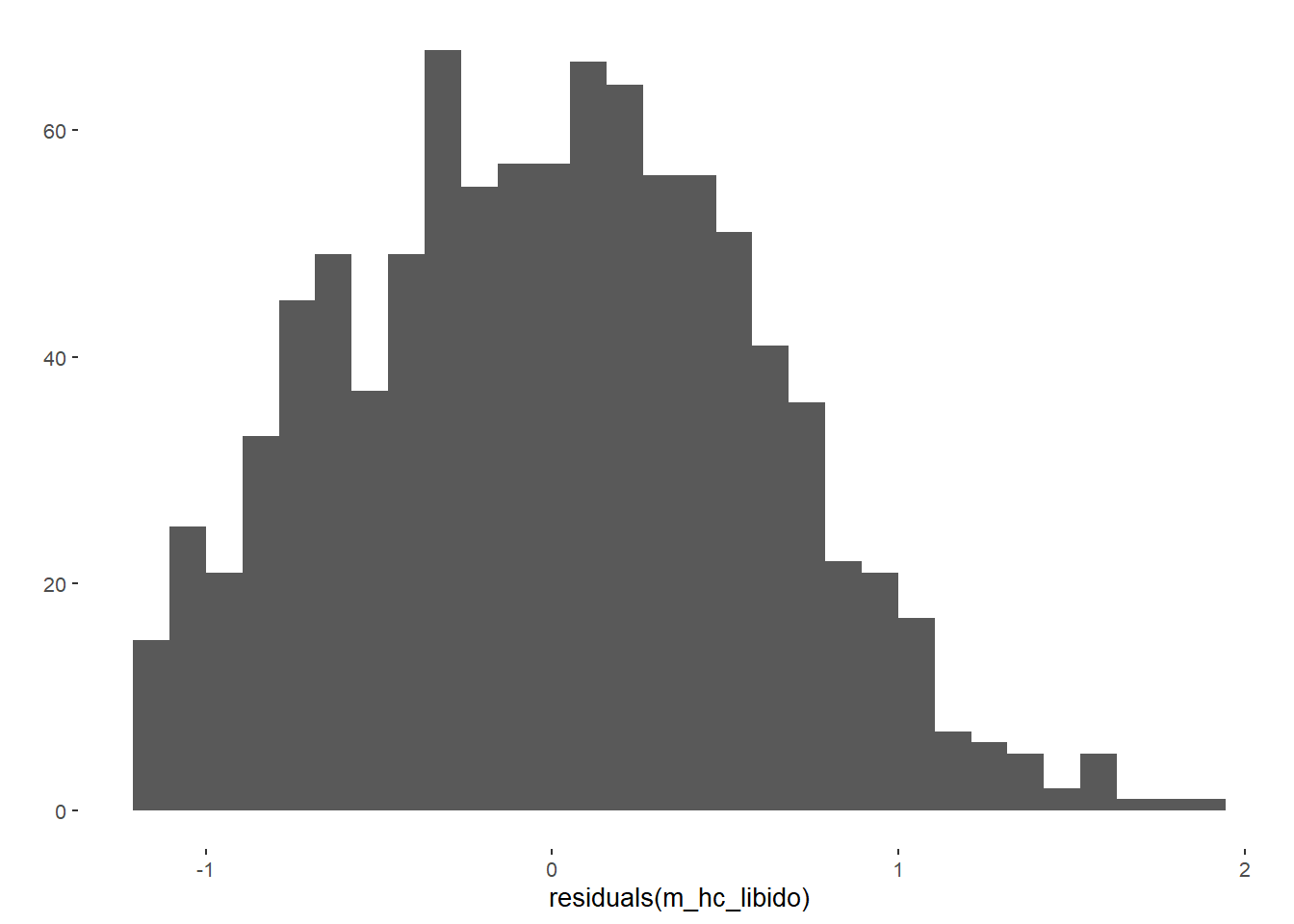
##
## Call:
## lm(formula = diary_libido_mean ~ contraception_hormonal_numeric,
##     data = data)
##
## Residuals:
##     Min      1Q  Median      3Q     Max
## -1.1999 -0.4392  0.0156  0.4217  1.8504
##
## Coefficients:
##                                Estimate Std. Error t value Pr(>|t|)
## (Intercept)                      1.1794     0.0244   48.43   <2e-16 ***
## contraception_hormonal_numeric   0.0205     0.0389    0.53      0.6
## ---
## Signif. codes:  0 '***' 0.001 '**' 0.01 '*' 0.05 '.' 0.1 ' ' 1
##
## Residual standard error: 0.591 on 966 degrees of freedom
##   (211 Beobachtungen als fehlend gelöscht)
## Multiple R-squared:  0.000286,   Adjusted R-squared:  -0.000749
## F-statistic: 0.276 on 1 and 966 DF, p-value: 0.599## # A tibble: 2 x 5
## term estimate std.error statistic p.value
## <chr> <dbl> <dbl> <dbl> <dbl>
## 1 (Intercept) 1.18 0.0244 48.4 1.21e-260
## 2 contraception_hormonal_numeric 0.0205 0.0389 0.526 5.99e- 1Sensitivity Analyses
m_hc_libido_sensitivity <- sensemakr(model = m_hc_libido, #model
                                treatment = "contraception_hormonal_numeric", #predictor
                                kd = 1:3, #these arguments parameterize how many times
                                          #stronger the confounder is related to the
                                          #treatment
                                ky = 1:3, #these arguments parameterize how many times
                                          #stronger the confounder is related to the outcome
                                q = 1, #fraction of the effect estimate that would have to be
                                       #explained away to be problematic. Setting q = 1,
                                       #means that a reduction of 100% of the current effect
                                       #estimate, that is, a true effect of zero, would be
                                       #deemed problematic.
                                alpha = 0.05,
                                reduce = TRUE #confounder reduce absolute effect size
                                )


m_hc_libido_sensitivity
## Sensitivity Analysis to Unobserved Confounding
##
## Model Formula: diary_libido_mean ~ contraception_hormonal_numeric
##
## Null hypothesis: q = 1 and reduce = TRUE
##
## Unadjusted Estimates of ' contraception_hormonal_numeric ':
## Coef. estimate: 0.02
## Standard Error: 0.039
## t-value: 0.526
##
## Sensitivity Statistics:
## Partial R2 of treatment with outcome: 0
## Robustness Value, q = 1 : 0.017
## Robustness Value, q = 1 alpha = 0.05 : 0
##
## For more information, check summary.## Sensitivity Analysis to Unobserved Confounding
##
## Model Formula: diary_libido_mean ~ contraception_hormonal_numeric
##
## Null hypothesis: q = 1 and reduce = TRUE
## -- This means we are considering biases that reduce the absolute value of the current estimate.
## -- The null hypothesis deemed problematic is H0:tau = 0
##
## Unadjusted Estimates of 'contraception_hormonal_numeric':
## Coef. estimate: 0.02
## Standard Error: 0.039
## t-value (H0:tau = 0): 0.526
##
## Sensitivity Statistics:
## Partial R2 of treatment with outcome: 0
## Robustness Value, q = 1: 0.017
## Robustness Value, q = 1, alpha = 0.05: 0
##
## Verbal interpretation of sensitivity statistics:
##
## -- Partial R2 of the treatment with the outcome: an extreme confounder (orthogonal to the covariates) that explains 100% of the residual variance of the outcome, would need to explain at least 0% of the residual variance of the treatment to fully account for the observed estimated effect.
##
## -- Robustness Value, q = 1: unobserved confounders (orthogonal to the covariates) that explain more than 1.7% of the residual variance of both the treatment and the outcome are strong enough to bring the point estimate to 0 (a bias of 100% of the original estimate). Conversely, unobserved confounders that do not explain more than 1.7% of the residual variance of both the treatment and the outcome are not strong enough to bring the point estimate to 0.
##
## -- Robustness Value, q = 1, alpha = 0.05: unobserved confounders (orthogonal to the covariates) that explain more than 0% of the residual variance of both the treatment and the outcome are strong enough to bring the estimate to a range where it is no longer 'statistically different' from 0 (a bias of 100% of the original estimate), at the significance level of alpha = 0.05. Conversely, unobserved confounders that do not explain more than 0% of the residual variance of both the treatment and the outcome are not strong enough to bring the estimate to a range where it is no longer 'statistically different' from 0, at the significance level of alpha = 0.05.Controlled Model
Model
m_hc_libido = lm(diary_libido_mean ~ contraception_hormonal_numeric +
                             age + net_income + relationship_duration_factor +
                              education_years +
                              bfi_extra + bfi_neuro + bfi_agree + bfi_consc + bfi_open +
                              religiosity,
               data = data)
summary(m_hc_libido)
##
## Call:
## lm(formula = diary_libido_mean ~ contraception_hormonal_numeric +
## age + net_income + relationship_duration_factor + education_years +
## bfi_extra + bfi_neuro + bfi_agree + bfi_consc + bfi_open +
## religiosity, data = data)
##
## Residuals:
## Min 1Q Median 3Q Max
## -1.2072 -0.4202 -0.0133 0.3861 2.1384
##
## Coefficients:
## Estimate Std. Error t value Pr(>|t|)
## (Intercept) 0.271018 0.260670 1.04 0.29875
## contraception_hormonal_numeric 0.006205 0.038723 0.16 0.87272
## age 0.003096 0.004850 0.64 0.52337
## net_incomeeuro_500_1000 0.097052 0.045213 2.15 0.03208 *
## net_incomeeuro_1000_2000 0.153580 0.063690 2.41 0.01608 *
## net_incomeeuro_2000_3000 0.099957 0.095511 1.05 0.29558
## net_incomeeuro_gt_3000 -0.057436 0.180229 -0.32 0.75004
## net_incomedont_tell 0.120695 0.122063 0.99 0.32302
## relationship_duration_factorPartnered_upto12months 0.411599 0.055502 7.42 2.7e-13 ***
## relationship_duration_factorPartnered_upto28months 0.305031 0.053421 5.71 1.5e-08 ***
## relationship_duration_factorPartnered_upto52months 0.245220 0.056750 4.32 1.7e-05 ***
## relationship_duration_factorPartnered_morethan52months 0.198792 0.059196 3.36 0.00082 ***
## education_years -0.000922 0.004072 -0.23 0.82100
## bfi_extra 0.089915 0.025736 3.49 0.00050 ***
## bfi_neuro -0.011547 0.027086 -0.43 0.66997
## bfi_agree 0.077788 0.033009 2.36 0.01864 *
## bfi_consc -0.101387 0.029166 -3.48 0.00053 ***
## bfi_open 0.104155 0.030626 3.40 0.00070 ***
## religiosity -0.007040 0.013734 -0.51 0.60836
## ---
## Signif. codes: 0 '***' 0.001 '**' 0.01 '*' 0.05 '.' 0.1 ' ' 1
##
## Residual standard error: 0.56 on 949 degrees of freedom
## (211 Beobachtungen als fehlend gelöscht)
## Multiple R-squared: 0.12, Adjusted R-squared: 0.103
## F-statistic: 7.16 on 18 and 949 DF, p-value: <2e-16## # A tibble: 19 x 5
## term estimate std.error statistic p.value
## <chr> <dbl> <dbl> <dbl> <dbl>
## 1 (Intercept) 0.271 0.261 1.04 2.99e- 1
## 2 contraception_hormonal_numeric 0.00621 0.0387 0.160 8.73e- 1
## 3 age 0.00310 0.00485 0.638 5.23e- 1
## 4 net_incomeeuro_500_1000 0.0971 0.0452 2.15 3.21e- 2
## 5 net_incomeeuro_1000_2000 0.154 0.0637 2.41 1.61e- 2
## 6 net_incomeeuro_2000_3000 0.100 0.0955 1.05 2.96e- 1
## 7 net_incomeeuro_gt_3000 -0.0574 0.180 -0.319 7.50e- 1
## 8 net_incomedont_tell 0.121 0.122 0.989 3.23e- 1
## 9 relationship_duration_factorPartnered_upto12months 0.412 0.0555 7.42 2.67e-13
## 10 relationship_duration_factorPartnered_upto28months 0.305 0.0534 5.71 1.51e- 8
## 11 relationship_duration_factorPartnered_upto52months 0.245 0.0567 4.32 1.72e- 5
## 12 relationship_duration_factorPartnered_morethan52months 0.199 0.0592 3.36 8.16e- 4
## 13 education_years -0.000922 0.00407 -0.226 8.21e- 1
## 14 bfi_extra 0.0899 0.0257 3.49 4.98e- 4
## 15 bfi_neuro -0.0115 0.0271 -0.426 6.70e- 1
## 16 bfi_agree 0.0778 0.0330 2.36 1.86e- 2
## 17 bfi_consc -0.101 0.0292 -3.48 5.32e- 4
## 18 bfi_open 0.104 0.0306 3.40 7.00e- 4
## 19 religiosity -0.00704 0.0137 -0.513 6.08e- 1Sensitivity Analyses
m_hc_libido_sensitivity <- sensemakr(model = m_hc_libido, #model
                                treatment = "contraception_hormonal_numeric", #predictor
                                benchmark_covariates = covariates, #covariates that will be
                                                                   #used to bound the
                                                                   #plausible strength of the
                                                                   #unobserved confounders
                                kd = 1:3, #these arguments parameterize how many times
                                          #stronger the confounder is related to the
                                          #treatment
                                ky = 1:3, #these arguments parameterize how many times
                                          #stronger the confounder is related to the outcome
                                q = 1, #fraction of the effect estimate that would have to be
                                       #explained away to be problematic. Setting q = 1,
                                       #means that a reduction of 100% of the current effect
                                       #estimate, that is, a true effect of zero, would be
                                       #deemed problematic.
                                alpha = 0.05,
                                reduce = TRUE #confounder reduce absolute effect size
                                )


m_hc_libido_sensitivity
## Sensitivity Analysis to Unobserved Confounding
##
## Model Formula: diary_libido_mean ~ contraception_hormonal_numeric + age + net_income +
## relationship_duration_factor + education_years + bfi_extra +
## bfi_neuro + bfi_agree + bfi_consc + bfi_open + religiosity
##
## Null hypothesis: q = 1 and reduce = TRUE
##
## Unadjusted Estimates of ' contraception_hormonal_numeric ':
## Coef. estimate: 0.006
## Standard Error: 0.039
## t-value: 0.16
##
## Sensitivity Statistics:
## Partial R2 of treatment with outcome: 0
## Robustness Value, q = 1 : 0.005
## Robustness Value, q = 1 alpha = 0.05 : 0
##
## For more information, check summary.## Sensitivity Analysis to Unobserved Confounding
##
## Model Formula: diary_libido_mean ~ contraception_hormonal_numeric + age + net_income +
## relationship_duration_factor + education_years + bfi_extra +
## bfi_neuro + bfi_agree + bfi_consc + bfi_open + religiosity
##
## Null hypothesis: q = 1 and reduce = TRUE
## -- This means we are considering biases that reduce the absolute value of the current estimate.
## -- The null hypothesis deemed problematic is H0:tau = 0
##
## Unadjusted Estimates of 'contraception_hormonal_numeric':
## Coef. estimate: 0.006
## Standard Error: 0.039
## t-value (H0:tau = 0): 0.16
##
## Sensitivity Statistics:
## Partial R2 of treatment with outcome: 0
## Robustness Value, q = 1: 0.005
## Robustness Value, q = 1, alpha = 0.05: 0
##
## Verbal interpretation of sensitivity statistics:
##
## -- Partial R2 of the treatment with the outcome: an extreme confounder (orthogonal to the covariates) that explains 100% of the residual variance of the outcome, would need to explain at least 0% of the residual variance of the treatment to fully account for the observed estimated effect.
##
## -- Robustness Value, q = 1: unobserved confounders (orthogonal to the covariates) that explain more than 0.5% of the residual variance of both the treatment and the outcome are strong enough to bring the point estimate to 0 (a bias of 100% of the original estimate). Conversely, unobserved confounders that do not explain more than 0.5% of the residual variance of both the treatment and the outcome are not strong enough to bring the point estimate to 0.
##
## -- Robustness Value, q = 1, alpha = 0.05: unobserved confounders (orthogonal to the covariates) that explain more than 0% of the residual variance of both the treatment and the outcome are strong enough to bring the estimate to a range where it is no longer 'statistically different' from 0 (a bias of 100% of the original estimate), at the significance level of alpha = 0.05. Conversely, unobserved confounders that do not explain more than 0% of the residual variance of both the treatment and the outcome are not strong enough to bring the estimate to a range where it is no longer 'statistically different' from 0, at the significance level of alpha = 0.05.
##
## Bounds on omitted variable bias:
##
## --The table below shows the maximum strength of unobserved confounders with association with the treatment and the outcome bounded by a multiple of the observed explanatory power of the chosen benchmark covariate(s).
##
## Bound Label R2dz.x R2yz.dx Treatment
## 1x age 0.031 0.000 contraception_hormonal_numeric
## 2x age 0.062 0.001 contraception_hormonal_numeric
## 3x age 0.093 0.001 contraception_hormonal_numeric
## 1x net_incomeeuro_500_1000 0.002 0.005 contraception_hormonal_numeric
## 2x net_incomeeuro_500_1000 0.003 0.010 contraception_hormonal_numeric
## 3x net_incomeeuro_500_1000 0.005 0.015 contraception_hormonal_numeric
## 1x net_incomeeuro_1000_2000 0.001 0.006 contraception_hormonal_numeric
## 2x net_incomeeuro_1000_2000 0.001 0.012 contraception_hormonal_numeric
## 3x net_incomeeuro_1000_2000 0.002 0.018 contraception_hormonal_numeric
## 1x net_incomeeuro_2000_3000 0.000 0.001 contraception_hormonal_numeric
## 2x net_incomeeuro_2000_3000 0.000 0.002 contraception_hormonal_numeric
## 3x net_incomeeuro_2000_3000 0.000 0.003 contraception_hormonal_numeric
## 1x net_incomeeuro_gt_3000 0.001 0.000 contraception_hormonal_numeric
## 2x net_incomeeuro_gt_3000 0.002 0.000 contraception_hormonal_numeric
## 3x net_incomeeuro_gt_3000 0.003 0.000 contraception_hormonal_numeric
## 1x net_incomedont_tell 0.000 0.001 contraception_hormonal_numeric
## 2x net_incomedont_tell 0.000 0.002 contraception_hormonal_numeric
## 3x net_incomedont_tell 0.000 0.003 contraception_hormonal_numeric
## 1x relationship_duration_factorPartnered_upto28months 0.020 0.036 contraception_hormonal_numeric
## 2x relationship_duration_factorPartnered_upto28months 0.039 0.072 contraception_hormonal_numeric
## 3x relationship_duration_factorPartnered_upto28months 0.059 0.107 contraception_hormonal_numeric
## 1x relationship_duration_factorPartnered_upto52months 0.017 0.020 contraception_hormonal_numeric
## 2x relationship_duration_factorPartnered_upto52months 0.035 0.041 contraception_hormonal_numeric
## 3x relationship_duration_factorPartnered_upto52months 0.052 0.061 contraception_hormonal_numeric
## 1x relationship_duration_factorPartnered_morethan52months 0.029 0.013 contraception_hormonal_numeric
## 2x relationship_duration_factorPartnered_morethan52months 0.057 0.025 contraception_hormonal_numeric
## 3x relationship_duration_factorPartnered_morethan52months 0.086 0.038 contraception_hormonal_numeric
## 1x education_years 0.001 0.000 contraception_hormonal_numeric
## 2x education_years 0.002 0.000 contraception_hormonal_numeric
## 3x education_years 0.004 0.000 contraception_hormonal_numeric
## 1x bfi_extra 0.001 0.013 contraception_hormonal_numeric
## 2x bfi_extra 0.002 0.026 contraception_hormonal_numeric
## 3x bfi_extra 0.003 0.039 contraception_hormonal_numeric
## 1x bfi_neuro 0.001 0.000 contraception_hormonal_numeric
## 2x bfi_neuro 0.003 0.000 contraception_hormonal_numeric
## 3x bfi_neuro 0.004 0.001 contraception_hormonal_numeric
## 1x bfi_agree 0.001 0.006 contraception_hormonal_numeric
## 2x bfi_agree 0.001 0.012 contraception_hormonal_numeric
## 3x bfi_agree 0.002 0.018 contraception_hormonal_numeric
## 1x bfi_consc 0.009 0.013 contraception_hormonal_numeric
## 2x bfi_consc 0.018 0.026 contraception_hormonal_numeric
## 3x bfi_consc 0.026 0.039 contraception_hormonal_numeric
## 1x bfi_open 0.006 0.012 contraception_hormonal_numeric
## 2x bfi_open 0.012 0.025 contraception_hormonal_numeric
## 3x bfi_open 0.018 0.037 contraception_hormonal_numeric
## 1x religiosity 0.001 0.000 contraception_hormonal_numeric
## 2x religiosity 0.003 0.001 contraception_hormonal_numeric
## 3x religiosity 0.004 0.001 contraception_hormonal_numeric
## Adjusted Estimate Adjusted Se Adjusted T Adjusted Lower CI Adjusted Upper CI
## 0.002 0.039 0.042 -0.076 0.079
## -0.003 0.040 -0.077 -0.082 0.075
## -0.008 0.041 -0.196 -0.088 0.072
## 0.003 0.039 0.071 -0.073 0.079
## -0.001 0.039 -0.019 -0.077 0.075
## -0.004 0.039 -0.109 -0.080 0.071
## 0.004 0.039 0.101 -0.072 0.080
## 0.002 0.039 0.042 -0.074 0.077
## -0.001 0.038 -0.018 -0.076 0.075
## 0.006 0.039 0.150 -0.070 0.082
## 0.005 0.039 0.140 -0.071 0.081
## 0.005 0.039 0.131 -0.071 0.081
## 0.006 0.039 0.151 -0.070 0.082
## 0.005 0.039 0.141 -0.071 0.082
## 0.005 0.039 0.132 -0.071 0.081
## 0.006 0.039 0.159 -0.070 0.082
## 0.006 0.039 0.158 -0.070 0.082
## 0.006 0.039 0.157 -0.070 0.082
## -0.026 0.038 -0.671 -0.101 0.050
## -0.058 0.038 -1.535 -0.133 0.016
## -0.092 0.038 -2.433 -0.166 -0.018
## -0.016 0.039 -0.425 -0.092 0.059
## -0.040 0.039 -1.024 -0.115 0.036
## -0.063 0.039 -1.635 -0.139 0.013
## -0.017 0.039 -0.429 -0.093 0.060
## -0.040 0.039 -1.027 -0.118 0.037
## -0.065 0.040 -1.634 -0.143 0.013
## 0.006 0.039 0.152 -0.070 0.082
## 0.006 0.039 0.144 -0.071 0.082
## 0.005 0.039 0.136 -0.071 0.081
## 0.002 0.039 0.044 -0.074 0.077
## -0.003 0.038 -0.073 -0.078 0.072
## -0.007 0.038 -0.192 -0.082 0.067
## 0.006 0.039 0.144 -0.071 0.082
## 0.005 0.039 0.128 -0.071 0.081
## 0.004 0.039 0.111 -0.072 0.080
## 0.004 0.039 0.099 -0.072 0.080
## 0.001 0.039 0.038 -0.074 0.077
## -0.001 0.038 -0.023 -0.076 0.075
## -0.007 0.039 -0.171 -0.082 0.069
## -0.020 0.039 -0.507 -0.095 0.056
## -0.033 0.038 -0.847 -0.108 0.043
## -0.004 0.039 -0.109 -0.080 0.072
## -0.015 0.038 -0.381 -0.090 0.061
## -0.025 0.038 -0.656 -0.100 0.050
## 0.005 0.039 0.141 -0.071 0.082
## 0.005 0.039 0.122 -0.071 0.081
## 0.004 0.039 0.103 -0.072 0.080Sexual Frequency
Uncontrolled Model
Model
m_hc_sexfreqpen = lm(diary_sex_active_sex_mean ~ contraception_hormonal_numeric,
               data = data)
qplot(residuals(m_hc_sexfreqpen))
## `stat_bin()` using `bins = 30`. Pick better value with `binwidth`.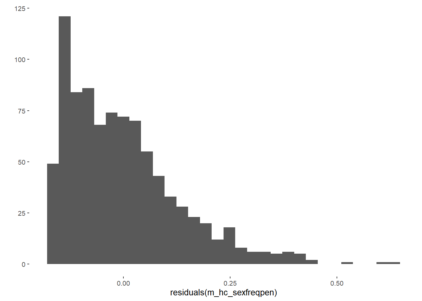
##
## Call:
## lm(formula = diary_sex_active_sex_mean ~ contraception_hormonal_numeric,
##     data = data)
##
## Residuals:
##     Min      1Q  Median      3Q     Max
## -0.1612 -0.1057 -0.0291  0.0650  0.6388
##
## Coefficients:
##                                Estimate Std. Error t value Pr(>|t|)
## (Intercept)                     0.12618    0.00575   21.94  < 2e-16 ***
## contraception_hormonal_numeric  0.03503    0.00885    3.96 0.000081 ***
## ---
## Signif. codes:  0 '***' 0.001 '**' 0.01 '*' 0.05 '.' 0.1 ' ' 1
##
## Residual standard error: 0.131 on 895 degrees of freedom
##   (282 Beobachtungen als fehlend gelöscht)
## Multiple R-squared:  0.0172, Adjusted R-squared:  0.0161
## F-statistic: 15.7 on 1 and 895 DF, p-value: 0.0000815## # A tibble: 2 x 7
## term estimate std.error statistic p.value conf.low conf.high
## <chr> <dbl> <dbl> <dbl> <dbl> <dbl> <dbl>
## 1 (Intercept) 0.126 0.00575 21.9 1.07e-85 0.115 0.137
## 2 contraception_hormonal_numeric 0.0350 0.00885 3.96 8.15e- 5 0.0177 0.0524Sensitivity Analyses
m_hc_sexfreqpen_sensitivity <- sensemakr(model = m_hc_sexfreqpen,
                                         treatment = "contraception_hormonal_numeric",
                                        kd = 1:3, #these arguments parameterize how many times
                                          #stronger the confounder is related to the
                                          #treatment
                                ky = 1:3, #these arguments parameterize how many times
                                          #stronger the confounder is related to the outcome
                                q = 1, #fraction of the effect estimate that would have to be
                                       #explained away to be problematic. Setting q = 1,
                                       #means that a reduction of 100% of the current effect
                                       #estimate, that is, a true effect of zero, would be
                                       #deemed problematic.
                                alpha = 0.05,
                                reduce = TRUE #confounder reduce absolute effect size
                                )


m_hc_sexfreqpen_sensitivity
## Sensitivity Analysis to Unobserved Confounding
##
## Model Formula: diary_sex_active_sex_mean ~ contraception_hormonal_numeric
##
## Null hypothesis: q = 1 and reduce = TRUE
##
## Unadjusted Estimates of ' contraception_hormonal_numeric ':
## Coef. estimate: 0.035
## Standard Error: 0.009
## t-value: 3.958
##
## Sensitivity Statistics:
## Partial R2 of treatment with outcome: 0.017
## Robustness Value, q = 1 : 0.124
## Robustness Value, q = 1 alpha = 0.05 : 0.064
##
## For more information, check summary.## Sensitivity Analysis to Unobserved Confounding
##
## Model Formula: diary_sex_active_sex_mean ~ contraception_hormonal_numeric
##
## Null hypothesis: q = 1 and reduce = TRUE
## -- This means we are considering biases that reduce the absolute value of the current estimate.
## -- The null hypothesis deemed problematic is H0:tau = 0
##
## Unadjusted Estimates of 'contraception_hormonal_numeric':
## Coef. estimate: 0.035
## Standard Error: 0.009
## t-value (H0:tau = 0): 3.958
##
## Sensitivity Statistics:
## Partial R2 of treatment with outcome: 0.017
## Robustness Value, q = 1: 0.124
## Robustness Value, q = 1, alpha = 0.05: 0.064
##
## Verbal interpretation of sensitivity statistics:
##
## -- Partial R2 of the treatment with the outcome: an extreme confounder (orthogonal to the covariates) that explains 100% of the residual variance of the outcome, would need to explain at least 1.7% of the residual variance of the treatment to fully account for the observed estimated effect.
##
## -- Robustness Value, q = 1: unobserved confounders (orthogonal to the covariates) that explain more than 12.4% of the residual variance of both the treatment and the outcome are strong enough to bring the point estimate to 0 (a bias of 100% of the original estimate). Conversely, unobserved confounders that do not explain more than 12.4% of the residual variance of both the treatment and the outcome are not strong enough to bring the point estimate to 0.
##
## -- Robustness Value, q = 1, alpha = 0.05: unobserved confounders (orthogonal to the covariates) that explain more than 6.4% of the residual variance of both the treatment and the outcome are strong enough to bring the estimate to a range where it is no longer 'statistically different' from 0 (a bias of 100% of the original estimate), at the significance level of alpha = 0.05. Conversely, unobserved confounders that do not explain more than 6.4% of the residual variance of both the treatment and the outcome are not strong enough to bring the estimate to a range where it is no longer 'statistically different' from 0, at the significance level of alpha = 0.05.Controlled Model
Model
m_hc_sexfreqpen = lm(diary_sex_active_sex_mean ~ contraception_hormonal_numeric +
                       age + net_income + relationship_duration_factor +
                              education_years +
                              bfi_extra + bfi_neuro + bfi_agree + bfi_consc + bfi_open +
                              religiosity,
               data = data)
qplot(residuals(m_hc_sexfreqpen))
## `stat_bin()` using `bins = 30`. Pick better value with `binwidth`.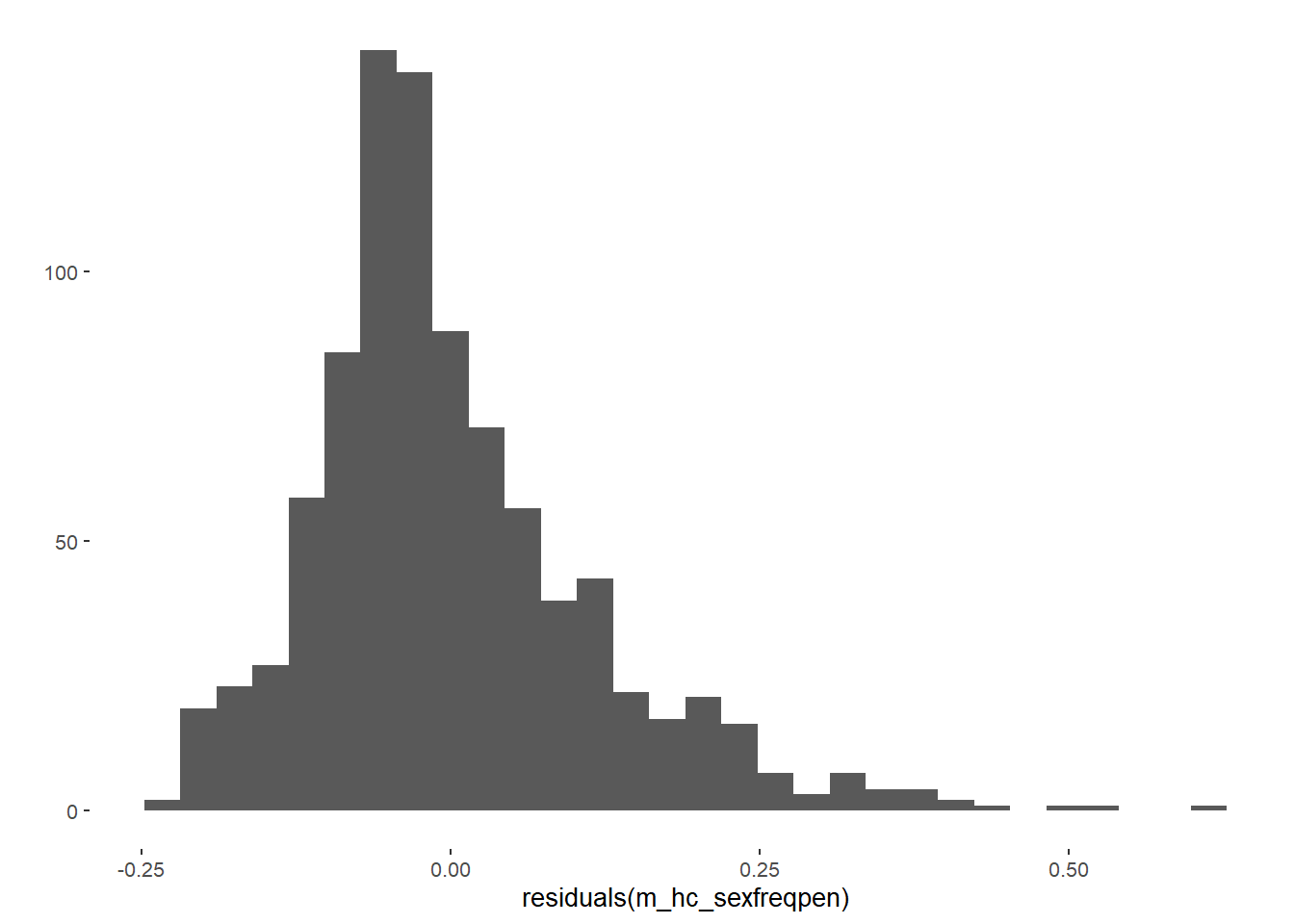
##
## Call:
## lm(formula = diary_sex_active_sex_mean ~ contraception_hormonal_numeric +
##     age + net_income + relationship_duration_factor + education_years +
##     bfi_extra + bfi_neuro + bfi_agree + bfi_consc + bfi_open +
##     religiosity, data = data)
##
## Residuals:
##     Min      1Q  Median      3Q     Max
## -0.2392 -0.0693 -0.0232  0.0530  0.6080
##
## Coefficients:
##                                                          Estimate Std. Error t value Pr(>|t|)
## (Intercept)                                            -0.0143402  0.0565191   -0.25   0.7998
## contraception_hormonal_numeric                          0.0242979  0.0082664    2.94   0.0034 **
## age                                                    -0.0000572  0.0010467   -0.05   0.9564
## net_incomeeuro_500_1000                                 0.0237180  0.0099392    2.39   0.0172 *
## net_incomeeuro_1000_2000                                0.0223460  0.0135506    1.65   0.0995 .
## net_incomeeuro_2000_3000                                0.0588764  0.0201520    2.92   0.0036 **
## net_incomeeuro_gt_3000                                  0.0029770  0.0376972    0.08   0.9371
## net_incomedont_tell                                     0.0718555  0.0271855    2.64   0.0084 **
## relationship_duration_factorPartnered_upto12months      0.1588406  0.0121142   13.11  < 2e-16 ***
## relationship_duration_factorPartnered_upto28months      0.1331838  0.0115110   11.57  < 2e-16 ***
## relationship_duration_factorPartnered_upto52months      0.0897725  0.0122027    7.36  4.3e-13 ***
## relationship_duration_factorPartnered_morethan52months  0.0889894  0.0125708    7.08  3.0e-12 ***
## education_years                                        -0.0012984  0.0008718   -1.49   0.1368
## bfi_extra                                               0.0015351  0.0055612    0.28   0.7826
## bfi_neuro                                               0.0010647  0.0058529    0.18   0.8557
## bfi_agree                                               0.0142641  0.0070948    2.01   0.0447 *
## bfi_consc                                              -0.0024751  0.0062501   -0.40   0.6922
## bfi_open                                                0.0047781  0.0065563    0.73   0.4663
## religiosity                                            -0.0029345  0.0030271   -0.97   0.3326
## ---
## Signif. codes:  0 '***' 0.001 '**' 0.01 '*' 0.05 '.' 0.1 ' ' 1
##
## Residual standard error: 0.117 on 878 degrees of freedom
##   (282 Beobachtungen als fehlend gelöscht)
## Multiple R-squared:  0.236,  Adjusted R-squared:  0.22
## F-statistic: 15.1 on 18 and 878 DF, p-value: <2e-16## # A tibble: 19 x 7
## term estimate std.error statistic p.value conf.low conf.high
## <chr> <dbl> <dbl> <dbl> <dbl> <dbl> <dbl>
## 1 (Intercept) -1.43e-2 0.0565 -0.254 8.00e- 1 -1.25e-1 0.0966
## 2 contraception_hormonal_numeric 2.43e-2 0.00827 2.94 3.38e- 3 8.07e-3 0.0405
## 3 age -5.72e-5 0.00105 -0.0547 9.56e- 1 -2.11e-3 0.00200
## 4 net_incomeeuro_500_1000 2.37e-2 0.00994 2.39 1.72e- 2 4.21e-3 0.0432
## 5 net_incomeeuro_1000_2000 2.23e-2 0.0136 1.65 9.95e- 2 -4.25e-3 0.0489
## 6 net_incomeeuro_2000_3000 5.89e-2 0.0202 2.92 3.57e- 3 1.93e-2 0.0984
## 7 net_incomeeuro_gt_3000 2.98e-3 0.0377 0.0790 9.37e- 1 -7.10e-2 0.0770
## 8 net_incomedont_tell 7.19e-2 0.0272 2.64 8.36e- 3 1.85e-2 0.125
## 9 relationship_duration_factorPartnered_upto12months 1.59e-1 0.0121 13.1 5.33e-36 1.35e-1 0.183
## 10 relationship_duration_factorPartnered_upto28months 1.33e-1 0.0115 11.6 6.47e-29 1.11e-1 0.156
## 11 relationship_duration_factorPartnered_upto52months 8.98e-2 0.0122 7.36 4.32e-13 6.58e-2 0.114
## 12 relationship_duration_factorPartnered_morethan52months 8.90e-2 0.0126 7.08 2.97e-12 6.43e-2 0.114
## 13 education_years -1.30e-3 0.000872 -1.49 1.37e- 1 -3.01e-3 0.000413
## 14 bfi_extra 1.54e-3 0.00556 0.276 7.83e- 1 -9.38e-3 0.0124
## 15 bfi_neuro 1.06e-3 0.00585 0.182 8.56e- 1 -1.04e-2 0.0126
## 16 bfi_agree 1.43e-2 0.00709 2.01 4.47e- 2 3.39e-4 0.0282
## 17 bfi_consc -2.48e-3 0.00625 -0.396 6.92e- 1 -1.47e-2 0.00979
## 18 bfi_open 4.78e-3 0.00656 0.729 4.66e- 1 -8.09e-3 0.0176
## 19 religiosity -2.93e-3 0.00303 -0.969 3.33e- 1 -8.88e-3 0.00301Sensitivity Analyses
m_hc_sexfreqpen_sensitivity <- sensemakr(model = m_hc_sexfreqpen,
                                         treatment = "contraception_hormonal_numeric",
                                         benchmark_covariates = covariates, #covariates that will be
                                                                   #used to bound the
                                                                   #plausible strength of the
                                                                   #unobserved confounders
                                kd = 1:3, #these arguments parameterize how many times
                                          #stronger the confounder is related to the
                                          #treatment
                                ky = 1:3, #these arguments parameterize how many times
                                          #stronger the confounder is related to the outcome
                                q = 1, #fraction of the effect estimate that would have to be
                                       #explained away to be problematic. Setting q = 1,
                                       #means that a reduction of 100% of the current effect
                                       #estimate, that is, a true effect of zero, would be
                                       #deemed problematic.
                                alpha = 0.05,
                                reduce = TRUE #confounder reduce absolute effect size
                                )


m_hc_sexfreqpen_sensitivity
## Sensitivity Analysis to Unobserved Confounding
##
## Model Formula: diary_sex_active_sex_mean ~ contraception_hormonal_numeric +
## age + net_income + relationship_duration_factor + education_years +
## bfi_extra + bfi_neuro + bfi_agree + bfi_consc + bfi_open +
## religiosity
##
## Null hypothesis: q = 1 and reduce = TRUE
##
## Unadjusted Estimates of ' contraception_hormonal_numeric ':
## Coef. estimate: 0.024
## Standard Error: 0.008
## t-value: 2.939
##
## Sensitivity Statistics:
## Partial R2 of treatment with outcome: 0.01
## Robustness Value, q = 1 : 0.094
## Robustness Value, q = 1 alpha = 0.05 : 0.032
##
## For more information, check summary.## Sensitivity Analysis to Unobserved Confounding
##
## Model Formula: diary_sex_active_sex_mean ~ contraception_hormonal_numeric +
## age + net_income + relationship_duration_factor + education_years +
## bfi_extra + bfi_neuro + bfi_agree + bfi_consc + bfi_open +
## religiosity
##
## Null hypothesis: q = 1 and reduce = TRUE
## -- This means we are considering biases that reduce the absolute value of the current estimate.
## -- The null hypothesis deemed problematic is H0:tau = 0
##
## Unadjusted Estimates of 'contraception_hormonal_numeric':
## Coef. estimate: 0.024
## Standard Error: 0.008
## t-value (H0:tau = 0): 2.939
##
## Sensitivity Statistics:
## Partial R2 of treatment with outcome: 0.01
## Robustness Value, q = 1: 0.094
## Robustness Value, q = 1, alpha = 0.05: 0.032
##
## Verbal interpretation of sensitivity statistics:
##
## -- Partial R2 of the treatment with the outcome: an extreme confounder (orthogonal to the covariates) that explains 100% of the residual variance of the outcome, would need to explain at least 1% of the residual variance of the treatment to fully account for the observed estimated effect.
##
## -- Robustness Value, q = 1: unobserved confounders (orthogonal to the covariates) that explain more than 9.4% of the residual variance of both the treatment and the outcome are strong enough to bring the point estimate to 0 (a bias of 100% of the original estimate). Conversely, unobserved confounders that do not explain more than 9.4% of the residual variance of both the treatment and the outcome are not strong enough to bring the point estimate to 0.
##
## -- Robustness Value, q = 1, alpha = 0.05: unobserved confounders (orthogonal to the covariates) that explain more than 3.2% of the residual variance of both the treatment and the outcome are strong enough to bring the estimate to a range where it is no longer 'statistically different' from 0 (a bias of 100% of the original estimate), at the significance level of alpha = 0.05. Conversely, unobserved confounders that do not explain more than 3.2% of the residual variance of both the treatment and the outcome are not strong enough to bring the estimate to a range where it is no longer 'statistically different' from 0, at the significance level of alpha = 0.05.
##
## Bounds on omitted variable bias:
##
## --The table below shows the maximum strength of unobserved confounders with association with the treatment and the outcome bounded by a multiple of the observed explanatory power of the chosen benchmark covariate(s).
##
## Bound Label R2dz.x R2yz.dx Treatment
## 1x age 0.031 0.000 contraception_hormonal_numeric
## 2x age 0.062 0.000 contraception_hormonal_numeric
## 3x age 0.093 0.000 contraception_hormonal_numeric
## 1x net_incomeeuro_500_1000 0.002 0.007 contraception_hormonal_numeric
## 2x net_incomeeuro_500_1000 0.003 0.013 contraception_hormonal_numeric
## 3x net_incomeeuro_500_1000 0.005 0.020 contraception_hormonal_numeric
## 1x net_incomeeuro_1000_2000 0.001 0.003 contraception_hormonal_numeric
## 2x net_incomeeuro_1000_2000 0.001 0.006 contraception_hormonal_numeric
## 3x net_incomeeuro_1000_2000 0.002 0.009 contraception_hormonal_numeric
## 1x net_incomeeuro_2000_3000 0.000 0.010 contraception_hormonal_numeric
## 2x net_incomeeuro_2000_3000 0.000 0.019 contraception_hormonal_numeric
## 3x net_incomeeuro_2000_3000 0.000 0.029 contraception_hormonal_numeric
## 1x net_incomeeuro_gt_3000 0.001 0.000 contraception_hormonal_numeric
## 2x net_incomeeuro_gt_3000 0.002 0.000 contraception_hormonal_numeric
## 3x net_incomeeuro_gt_3000 0.003 0.000 contraception_hormonal_numeric
## 1x net_incomedont_tell 0.000 0.008 contraception_hormonal_numeric
## 2x net_incomedont_tell 0.000 0.016 contraception_hormonal_numeric
## 3x net_incomedont_tell 0.000 0.024 contraception_hormonal_numeric
## 1x relationship_duration_factorPartnered_upto28months 0.020 0.159 contraception_hormonal_numeric
## 2x relationship_duration_factorPartnered_upto28months 0.039 0.317 contraception_hormonal_numeric
## 3x relationship_duration_factorPartnered_upto28months 0.059 0.477 contraception_hormonal_numeric
## 1x relationship_duration_factorPartnered_upto52months 0.017 0.064 contraception_hormonal_numeric
## 2x relationship_duration_factorPartnered_upto52months 0.035 0.128 contraception_hormonal_numeric
## 3x relationship_duration_factorPartnered_upto52months 0.052 0.192 contraception_hormonal_numeric
## 1x relationship_duration_factorPartnered_morethan52months 0.029 0.060 contraception_hormonal_numeric
## 2x relationship_duration_factorPartnered_morethan52months 0.057 0.121 contraception_hormonal_numeric
## 3x relationship_duration_factorPartnered_morethan52months 0.086 0.182 contraception_hormonal_numeric
## 1x education_years 0.001 0.003 contraception_hormonal_numeric
## 2x education_years 0.002 0.005 contraception_hormonal_numeric
## 3x education_years 0.004 0.008 contraception_hormonal_numeric
## 1x bfi_extra 0.001 0.000 contraception_hormonal_numeric
## 2x bfi_extra 0.002 0.000 contraception_hormonal_numeric
## 3x bfi_extra 0.003 0.000 contraception_hormonal_numeric
## 1x bfi_neuro 0.001 0.000 contraception_hormonal_numeric
## 2x bfi_neuro 0.003 0.000 contraception_hormonal_numeric
## 3x bfi_neuro 0.004 0.000 contraception_hormonal_numeric
## 1x bfi_agree 0.001 0.005 contraception_hormonal_numeric
## 2x bfi_agree 0.001 0.009 contraception_hormonal_numeric
## 3x bfi_agree 0.002 0.014 contraception_hormonal_numeric
## 1x bfi_consc 0.009 0.000 contraception_hormonal_numeric
## 2x bfi_consc 0.018 0.000 contraception_hormonal_numeric
## 3x bfi_consc 0.026 0.001 contraception_hormonal_numeric
## 1x bfi_open 0.006 0.001 contraception_hormonal_numeric
## 2x bfi_open 0.012 0.001 contraception_hormonal_numeric
## 3x bfi_open 0.018 0.002 contraception_hormonal_numeric
## 1x religiosity 0.001 0.001 contraception_hormonal_numeric
## 2x religiosity 0.003 0.002 contraception_hormonal_numeric
## 3x religiosity 0.004 0.003 contraception_hormonal_numeric
## Adjusted Estimate Adjusted Se Adjusted T Adjusted Lower CI Adjusted Upper CI
## 0.024 0.008 2.882 0.008 0.041
## 0.024 0.009 2.825 0.007 0.041
## 0.024 0.009 2.768 0.007 0.041
## 0.023 0.008 2.845 0.007 0.040
## 0.023 0.008 2.752 0.006 0.039
## 0.022 0.008 2.658 0.006 0.038
## 0.024 0.008 2.901 0.008 0.040
## 0.024 0.008 2.864 0.007 0.040
## 0.023 0.008 2.826 0.007 0.039
## 0.024 0.008 2.924 0.008 0.040
## 0.024 0.008 2.910 0.008 0.040
## 0.024 0.008 2.896 0.008 0.040
## 0.024 0.008 2.934 0.008 0.041
## 0.024 0.008 2.931 0.008 0.041
## 0.024 0.008 2.927 0.008 0.040
## 0.024 0.008 2.946 0.008 0.040
## 0.024 0.008 2.955 0.008 0.040
## 0.024 0.008 2.964 0.008 0.040
## 0.010 0.008 1.365 -0.005 0.026
## -0.004 0.007 -0.526 -0.017 0.010
## -0.018 0.006 -2.935 -0.030 -0.006
## 0.016 0.008 1.989 0.000 0.032
## 0.008 0.008 0.976 -0.008 0.023
## -0.001 0.008 -0.115 -0.016 0.014
## 0.014 0.008 1.716 -0.002 0.030
## 0.003 0.008 0.412 -0.012 0.019
## -0.008 0.008 -0.988 -0.023 0.008
## 0.024 0.008 2.888 0.008 0.040
## 0.023 0.008 2.838 0.007 0.040
## 0.023 0.008 2.788 0.007 0.039
## 0.024 0.008 2.927 0.008 0.040
## 0.024 0.008 2.916 0.008 0.040
## 0.024 0.008 2.906 0.008 0.040
## 0.024 0.008 2.929 0.008 0.040
## 0.024 0.008 2.920 0.008 0.040
## 0.024 0.008 2.911 0.008 0.040
## 0.024 0.008 2.891 0.008 0.040
## 0.023 0.008 2.845 0.007 0.040
## 0.023 0.008 2.798 0.007 0.039
## 0.024 0.008 2.887 0.008 0.040
## 0.024 0.008 2.837 0.007 0.040
## 0.023 0.008 2.787 0.007 0.040
## 0.024 0.008 2.872 0.008 0.040
## 0.023 0.008 2.807 0.007 0.040
## 0.023 0.008 2.741 0.006 0.039
## 0.024 0.008 2.901 0.008 0.040
## 0.024 0.008 2.865 0.007 0.040
## 0.023 0.008 2.828 0.007 0.040Masturbation Frequency
Uncontrolled Model
Model
m_hc_masfreqpen = lm(diary_masturbation_mean ~ contraception_hormonal_numeric,
                     data = data)
qplot(residuals(m_hc_masfreqpen))
## `stat_bin()` using `bins = 30`. Pick better value with `binwidth`.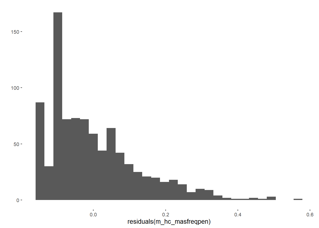
##
## Call:
## lm(formula = diary_masturbation_mean ~ contraception_hormonal_numeric,
##     data = data)
##
## Residuals:
##     Min      1Q  Median      3Q     Max
## -0.1530 -0.1022 -0.0318  0.0657  0.5613
##
## Coefficients:
##                                Estimate Std. Error t value   Pr(>|t|)
## (Intercept)                     0.15302    0.00557   27.49    < 2e-16 ***
## contraception_hormonal_numeric -0.04400    0.00857   -5.14 0.00000034 ***
## ---
## Signif. codes:  0 '***' 0.001 '**' 0.01 '*' 0.05 '.' 0.1 ' ' 1
##
## Residual standard error: 0.127 on 895 degrees of freedom
##   (282 Beobachtungen als fehlend gelöscht)
## Multiple R-squared:  0.0286, Adjusted R-squared:  0.0276
## F-statistic: 26.4 on 1 and 895 DF, p-value: 0.000000343## # A tibble: 2 x 7
## term estimate std.error statistic p.value conf.low conf.high
## <chr> <dbl> <dbl> <dbl> <dbl> <dbl> <dbl>
## 1 (Intercept) 0.153 0.00557 27.5 4.55e-121 0.142 0.164
## 2 contraception_hormonal_numeric -0.0440 0.00857 -5.14 3.43e- 7 -0.0608 -0.0272Sensitivity Analyses
m_hc_masfreqpen_sensitivity <- sensemakr(model = m_hc_masfreqpen,
                                         treatment = "contraception_hormonal_numeric",
                                         kd = 1:3, #these arguments parameterize how many times
                                         #stronger the confounder is related to the
                                         #treatment
                                         ky = 1:3, #these arguments parameterize how many times
                                         #stronger the confounder is related to the outcome
                                         q = 1, #fraction of the effect estimate that would have to be
                                         #explained away to be problematic. Setting q = 1,
                                         #means that a reduction of 100% of the current effect
                                         #estimate, that is, a true effect of zero, would be
                                         #deemed problematic.
                                         alpha = 0.05,
                                         reduce = TRUE #confounder reduce absolute effect size
)


m_hc_masfreqpen_sensitivity
## Sensitivity Analysis to Unobserved Confounding
##
## Model Formula: diary_masturbation_mean ~ contraception_hormonal_numeric
##
## Null hypothesis: q = 1 and reduce = TRUE
##
## Unadjusted Estimates of ' contraception_hormonal_numeric ':
## Coef. estimate: -0.044
## Standard Error: 0.009
## t-value: -5.137
##
## Sensitivity Statistics:
## Partial R2 of treatment with outcome: 0.029
## Robustness Value, q = 1 : 0.158
## Robustness Value, q = 1 alpha = 0.05 : 0.101
##
## For more information, check summary.## Sensitivity Analysis to Unobserved Confounding
##
## Model Formula: diary_masturbation_mean ~ contraception_hormonal_numeric
##
## Null hypothesis: q = 1 and reduce = TRUE
## -- This means we are considering biases that reduce the absolute value of the current estimate.
## -- The null hypothesis deemed problematic is H0:tau = 0
##
## Unadjusted Estimates of 'contraception_hormonal_numeric':
## Coef. estimate: -0.044
## Standard Error: 0.009
## t-value (H0:tau = 0): -5.137
##
## Sensitivity Statistics:
## Partial R2 of treatment with outcome: 0.029
## Robustness Value, q = 1: 0.158
## Robustness Value, q = 1, alpha = 0.05: 0.101
##
## Verbal interpretation of sensitivity statistics:
##
## -- Partial R2 of the treatment with the outcome: an extreme confounder (orthogonal to the covariates) that explains 100% of the residual variance of the outcome, would need to explain at least 2.9% of the residual variance of the treatment to fully account for the observed estimated effect.
##
## -- Robustness Value, q = 1: unobserved confounders (orthogonal to the covariates) that explain more than 15.8% of the residual variance of both the treatment and the outcome are strong enough to bring the point estimate to 0 (a bias of 100% of the original estimate). Conversely, unobserved confounders that do not explain more than 15.8% of the residual variance of both the treatment and the outcome are not strong enough to bring the point estimate to 0.
##
## -- Robustness Value, q = 1, alpha = 0.05: unobserved confounders (orthogonal to the covariates) that explain more than 10.1% of the residual variance of both the treatment and the outcome are strong enough to bring the estimate to a range where it is no longer 'statistically different' from 0 (a bias of 100% of the original estimate), at the significance level of alpha = 0.05. Conversely, unobserved confounders that do not explain more than 10.1% of the residual variance of both the treatment and the outcome are not strong enough to bring the estimate to a range where it is no longer 'statistically different' from 0, at the significance level of alpha = 0.05.Controlled Model
Model
m_hc_masfreqpen = lm(diary_masturbation_mean ~ contraception_hormonal_numeric +
                       age + net_income + relationship_duration_factor +
                       education_years +
                       bfi_extra + bfi_neuro + bfi_agree + bfi_consc + bfi_open +
                       religiosity,
                     data = data)
qplot(residuals(m_hc_masfreqpen))
## `stat_bin()` using `bins = 30`. Pick better value with `binwidth`.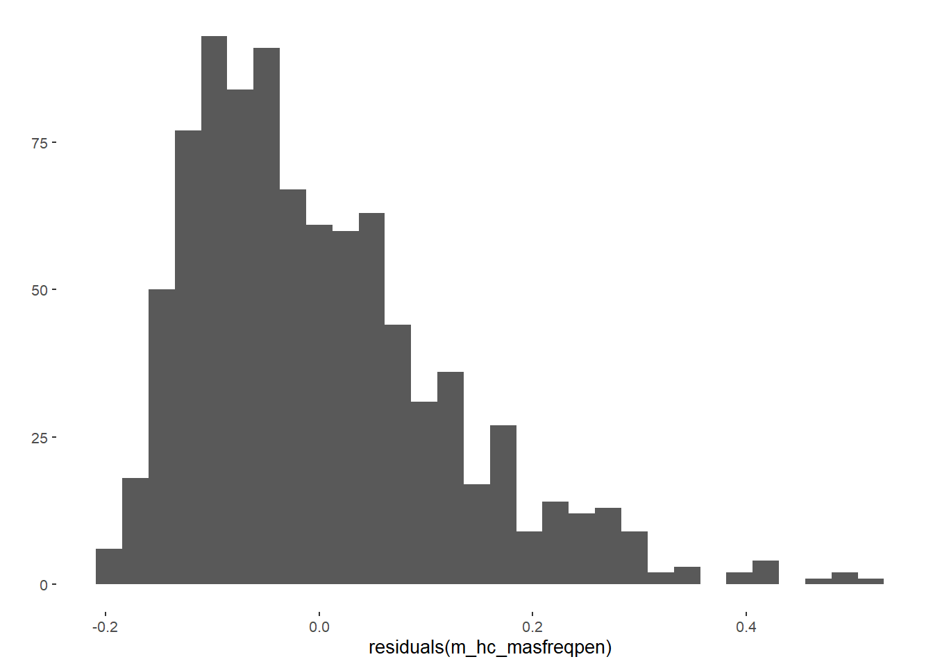
##
## Call:
## lm(formula = diary_masturbation_mean ~ contraception_hormonal_numeric +
##     age + net_income + relationship_duration_factor + education_years +
##     bfi_extra + bfi_neuro + bfi_agree + bfi_consc + bfi_open +
##     religiosity, data = data)
##
## Residuals:
##     Min      1Q  Median      3Q     Max
## -0.2071 -0.0913 -0.0243  0.0626  0.5066
##
## Coefficients:
##                                                         Estimate Std. Error t value Pr(>|t|)
## (Intercept)                                             0.157828   0.059203    2.67  0.00782 **
## contraception_hormonal_numeric                         -0.030214   0.008659   -3.49  0.00051 ***
## age                                                    -0.000254   0.001096   -0.23  0.81656
## net_incomeeuro_500_1000                                 0.021950   0.010411    2.11  0.03529 *
## net_incomeeuro_1000_2000                                0.024486   0.014194    1.73  0.08486 .
## net_incomeeuro_2000_3000                                0.004093   0.021109    0.19  0.84630
## net_incomeeuro_gt_3000                                 -0.026282   0.039487   -0.67  0.50585
## net_incomedont_tell                                    -0.025931   0.028476   -0.91  0.36275
## relationship_duration_factorPartnered_upto12months     -0.038676   0.012689   -3.05  0.00237 **
## relationship_duration_factorPartnered_upto28months     -0.036645   0.012058   -3.04  0.00244 **
## relationship_duration_factorPartnered_upto52months     -0.041856   0.012782   -3.27  0.00110 **
## relationship_duration_factorPartnered_morethan52months -0.054834   0.013168   -4.16 0.000034 ***
## education_years                                         0.000374   0.000913    0.41  0.68237
## bfi_extra                                              -0.001884   0.005825   -0.32  0.74650
## bfi_neuro                                              -0.001935   0.006131   -0.32  0.75233
## bfi_agree                                               0.000556   0.007432    0.07  0.94037
## bfi_consc                                              -0.023943   0.006547   -3.66  0.00027 ***
## bfi_open                                                0.030427   0.006868    4.43 0.000011 ***
## religiosity                                            -0.006685   0.003171   -2.11  0.03529 *
## ---
## Signif. codes:  0 '***' 0.001 '**' 0.01 '*' 0.05 '.' 0.1 ' ' 1
##
## Residual standard error: 0.122 on 878 degrees of freedom
##   (282 Beobachtungen als fehlend gelöscht)
## Multiple R-squared:  0.116,  Adjusted R-squared:  0.0977
## F-statistic: 6.39 on 18 and 878 DF, p-value: 4.79e-15## # A tibble: 19 x 7
## term estimate std.error statistic p.value conf.low conf.high
## <chr> <dbl> <dbl> <dbl> <dbl> <dbl> <dbl>
## 1 (Intercept) 1.58e-1 0.0592 2.67 7.82e-3 0.0416 0.274
## 2 contraception_hormonal_numeric -3.02e-2 0.00866 -3.49 5.08e-4 -0.0472 -0.0132
## 3 age -2.54e-4 0.00110 -0.232 8.17e-1 -0.00241 0.00190
## 4 net_incomeeuro_500_1000 2.19e-2 0.0104 2.11 3.53e-2 0.00152 0.0424
## 5 net_incomeeuro_1000_2000 2.45e-2 0.0142 1.73 8.49e-2 -0.00337 0.0523
## 6 net_incomeeuro_2000_3000 4.09e-3 0.0211 0.194 8.46e-1 -0.0373 0.0455
## 7 net_incomeeuro_gt_3000 -2.63e-2 0.0395 -0.666 5.06e-1 -0.104 0.0512
## 8 net_incomedont_tell -2.59e-2 0.0285 -0.911 3.63e-1 -0.0818 0.0300
## 9 relationship_duration_factorPartnered_upto12months -3.87e-2 0.0127 -3.05 2.37e-3 -0.0636 -0.0138
## 10 relationship_duration_factorPartnered_upto28months -3.66e-2 0.0121 -3.04 2.44e-3 -0.0603 -0.0130
## 11 relationship_duration_factorPartnered_upto52months -4.19e-2 0.0128 -3.27 1.10e-3 -0.0669 -0.0168
## 12 relationship_duration_factorPartnered_morethan52months -5.48e-2 0.0132 -4.16 3.43e-5 -0.0807 -0.0290
## 13 education_years 3.74e-4 0.000913 0.409 6.82e-1 -0.00142 0.00217
## 14 bfi_extra -1.88e-3 0.00583 -0.323 7.47e-1 -0.0133 0.00955
## 15 bfi_neuro -1.94e-3 0.00613 -0.316 7.52e-1 -0.0140 0.0101
## 16 bfi_agree 5.56e-4 0.00743 0.0748 9.40e-1 -0.0140 0.0151
## 17 bfi_consc -2.39e-2 0.00655 -3.66 2.70e-4 -0.0368 -0.0111
## 18 bfi_open 3.04e-2 0.00687 4.43 1.06e-5 0.0169 0.0439
## 19 religiosity -6.68e-3 0.00317 -2.11 3.53e-2 -0.0129 -0.000462Sensitivity Analyses
m_hc_masfreqpen_sensitivity <- sensemakr(model = m_hc_masfreqpen,
                                         treatment = "contraception_hormonal_numeric",
                                         benchmark_covariates = covariates, #covariates that will be
                                         #used to bound the
                                         #plausible strength of the
                                         #unobserved confounders
                                         kd = 1:3, #these arguments parameterize how many times
                                         #stronger the confounder is related to the
                                         #treatment
                                         ky = 1:3, #these arguments parameterize how many times
                                         #stronger the confounder is related to the outcome
                                         q = 1, #fraction of the effect estimate that would have to be
                                         #explained away to be problematic. Setting q = 1,
                                         #means that a reduction of 100% of the current effect
                                         #estimate, that is, a true effect of zero, would be
                                         #deemed problematic.
                                         alpha = 0.05,
                                         reduce = TRUE #confounder reduce absolute effect size
)


m_hc_masfreqpen_sensitivity
## Sensitivity Analysis to Unobserved Confounding
##
## Model Formula: diary_masturbation_mean ~ contraception_hormonal_numeric + age +
## net_income + relationship_duration_factor + education_years +
## bfi_extra + bfi_neuro + bfi_agree + bfi_consc + bfi_open +
## religiosity
##
## Null hypothesis: q = 1 and reduce = TRUE
##
## Unadjusted Estimates of ' contraception_hormonal_numeric ':
## Coef. estimate: -0.03
## Standard Error: 0.009
## t-value: -3.489
##
## Sensitivity Statistics:
## Partial R2 of treatment with outcome: 0.014
## Robustness Value, q = 1 : 0.111
## Robustness Value, q = 1 alpha = 0.05 : 0.05
##
## For more information, check summary.## Sensitivity Analysis to Unobserved Confounding
##
## Model Formula: diary_masturbation_mean ~ contraception_hormonal_numeric + age +
## net_income + relationship_duration_factor + education_years +
## bfi_extra + bfi_neuro + bfi_agree + bfi_consc + bfi_open +
## religiosity
##
## Null hypothesis: q = 1 and reduce = TRUE
## -- This means we are considering biases that reduce the absolute value of the current estimate.
## -- The null hypothesis deemed problematic is H0:tau = 0
##
## Unadjusted Estimates of 'contraception_hormonal_numeric':
## Coef. estimate: -0.03
## Standard Error: 0.009
## t-value (H0:tau = 0): -3.489
##
## Sensitivity Statistics:
## Partial R2 of treatment with outcome: 0.014
## Robustness Value, q = 1: 0.111
## Robustness Value, q = 1, alpha = 0.05: 0.05
##
## Verbal interpretation of sensitivity statistics:
##
## -- Partial R2 of the treatment with the outcome: an extreme confounder (orthogonal to the covariates) that explains 100% of the residual variance of the outcome, would need to explain at least 1.4% of the residual variance of the treatment to fully account for the observed estimated effect.
##
## -- Robustness Value, q = 1: unobserved confounders (orthogonal to the covariates) that explain more than 11.1% of the residual variance of both the treatment and the outcome are strong enough to bring the point estimate to 0 (a bias of 100% of the original estimate). Conversely, unobserved confounders that do not explain more than 11.1% of the residual variance of both the treatment and the outcome are not strong enough to bring the point estimate to 0.
##
## -- Robustness Value, q = 1, alpha = 0.05: unobserved confounders (orthogonal to the covariates) that explain more than 5% of the residual variance of both the treatment and the outcome are strong enough to bring the estimate to a range where it is no longer 'statistically different' from 0 (a bias of 100% of the original estimate), at the significance level of alpha = 0.05. Conversely, unobserved confounders that do not explain more than 5% of the residual variance of both the treatment and the outcome are not strong enough to bring the estimate to a range where it is no longer 'statistically different' from 0, at the significance level of alpha = 0.05.
##
## Bounds on omitted variable bias:
##
## --The table below shows the maximum strength of unobserved confounders with association with the treatment and the outcome bounded by a multiple of the observed explanatory power of the chosen benchmark covariate(s).
##
## Bound Label R2dz.x R2yz.dx Treatment
## 1x age 0.031 0.000 contraception_hormonal_numeric
## 2x age 0.062 0.000 contraception_hormonal_numeric
## 3x age 0.093 0.000 contraception_hormonal_numeric
## 1x net_incomeeuro_500_1000 0.002 0.005 contraception_hormonal_numeric
## 2x net_incomeeuro_500_1000 0.003 0.010 contraception_hormonal_numeric
## 3x net_incomeeuro_500_1000 0.005 0.015 contraception_hormonal_numeric
## 1x net_incomeeuro_1000_2000 0.001 0.003 contraception_hormonal_numeric
## 2x net_incomeeuro_1000_2000 0.001 0.007 contraception_hormonal_numeric
## 3x net_incomeeuro_1000_2000 0.002 0.010 contraception_hormonal_numeric
## 1x net_incomeeuro_2000_3000 0.000 0.000 contraception_hormonal_numeric
## 2x net_incomeeuro_2000_3000 0.000 0.000 contraception_hormonal_numeric
## 3x net_incomeeuro_2000_3000 0.000 0.000 contraception_hormonal_numeric
## 1x net_incomeeuro_gt_3000 0.001 0.001 contraception_hormonal_numeric
## 2x net_incomeeuro_gt_3000 0.002 0.001 contraception_hormonal_numeric
## 3x net_incomeeuro_gt_3000 0.003 0.002 contraception_hormonal_numeric
## 1x net_incomedont_tell 0.000 0.001 contraception_hormonal_numeric
## 2x net_incomedont_tell 0.000 0.002 contraception_hormonal_numeric
## 3x net_incomedont_tell 0.000 0.003 contraception_hormonal_numeric
## 1x relationship_duration_factorPartnered_upto28months 0.020 0.011 contraception_hormonal_numeric
## 2x relationship_duration_factorPartnered_upto28months 0.039 0.022 contraception_hormonal_numeric
## 3x relationship_duration_factorPartnered_upto28months 0.059 0.033 contraception_hormonal_numeric
## 1x relationship_duration_factorPartnered_upto52months 0.017 0.013 contraception_hormonal_numeric
## 2x relationship_duration_factorPartnered_upto52months 0.035 0.025 contraception_hormonal_numeric
## 3x relationship_duration_factorPartnered_upto52months 0.052 0.038 contraception_hormonal_numeric
## 1x relationship_duration_factorPartnered_morethan52months 0.029 0.021 contraception_hormonal_numeric
## 2x relationship_duration_factorPartnered_morethan52months 0.057 0.042 contraception_hormonal_numeric
## 3x relationship_duration_factorPartnered_morethan52months 0.086 0.063 contraception_hormonal_numeric
## 1x education_years 0.001 0.000 contraception_hormonal_numeric
## 2x education_years 0.002 0.000 contraception_hormonal_numeric
## 3x education_years 0.004 0.001 contraception_hormonal_numeric
## 1x bfi_extra 0.001 0.000 contraception_hormonal_numeric
## 2x bfi_extra 0.002 0.000 contraception_hormonal_numeric
## 3x bfi_extra 0.003 0.000 contraception_hormonal_numeric
## 1x bfi_neuro 0.001 0.000 contraception_hormonal_numeric
## 2x bfi_neuro 0.003 0.000 contraception_hormonal_numeric
## 3x bfi_neuro 0.004 0.000 contraception_hormonal_numeric
## 1x bfi_agree 0.001 0.000 contraception_hormonal_numeric
## 2x bfi_agree 0.001 0.000 contraception_hormonal_numeric
## 3x bfi_agree 0.002 0.000 contraception_hormonal_numeric
## 1x bfi_consc 0.009 0.016 contraception_hormonal_numeric
## 2x bfi_consc 0.018 0.031 contraception_hormonal_numeric
## 3x bfi_consc 0.026 0.047 contraception_hormonal_numeric
## 1x bfi_open 0.006 0.023 contraception_hormonal_numeric
## 2x bfi_open 0.012 0.045 contraception_hormonal_numeric
## 3x bfi_open 0.018 0.068 contraception_hormonal_numeric
## 1x religiosity 0.001 0.005 contraception_hormonal_numeric
## 2x religiosity 0.003 0.010 contraception_hormonal_numeric
## 3x religiosity 0.004 0.015 contraception_hormonal_numeric
## Adjusted Estimate Adjusted Se Adjusted T Adjusted Lower CI Adjusted Upper CI
## -0.030 0.009 -3.391 -0.047 -0.013
## -0.029 0.009 -3.293 -0.047 -0.012
## -0.029 0.009 -3.194 -0.047 -0.011
## -0.029 0.009 -3.405 -0.046 -0.012
## -0.029 0.009 -3.323 -0.046 -0.012
## -0.028 0.009 -3.239 -0.045 -0.011
## -0.030 0.009 -3.450 -0.047 -0.013
## -0.029 0.009 -3.412 -0.046 -0.013
## -0.029 0.009 -3.374 -0.046 -0.012
## -0.030 0.009 -3.485 -0.047 -0.013
## -0.030 0.009 -3.483 -0.047 -0.013
## -0.030 0.009 -3.482 -0.047 -0.013
## -0.030 0.009 -3.467 -0.047 -0.013
## -0.030 0.009 -3.447 -0.047 -0.013
## -0.030 0.009 -3.427 -0.047 -0.013
## -0.030 0.009 -3.488 -0.047 -0.013
## -0.030 0.009 -3.489 -0.047 -0.013
## -0.030 0.009 -3.489 -0.047 -0.013
## -0.026 0.009 -3.034 -0.043 -0.009
## -0.023 0.009 -2.576 -0.040 -0.005
## -0.019 0.009 -2.111 -0.036 -0.001
## -0.026 0.009 -3.037 -0.043 -0.009
## -0.022 0.009 -2.580 -0.040 -0.005
## -0.018 0.009 -2.117 -0.036 -0.001
## -0.024 0.009 -2.741 -0.041 -0.007
## -0.017 0.009 -1.977 -0.034 0.000
## -0.010 0.009 -1.195 -0.028 0.007
## -0.030 0.009 -3.471 -0.047 -0.013
## -0.030 0.009 -3.455 -0.047 -0.013
## -0.030 0.009 -3.440 -0.047 -0.013
## -0.030 0.009 -3.475 -0.047 -0.013
## -0.030 0.009 -3.462 -0.047 -0.013
## -0.030 0.009 -3.450 -0.047 -0.013
## -0.030 0.009 -3.473 -0.047 -0.013
## -0.030 0.009 -3.459 -0.047 -0.013
## -0.030 0.009 -3.445 -0.047 -0.013
## -0.030 0.009 -3.484 -0.047 -0.013
## -0.030 0.009 -3.481 -0.047 -0.013
## -0.030 0.009 -3.478 -0.047 -0.013
## -0.027 0.009 -3.150 -0.044 -0.010
## -0.024 0.009 -2.807 -0.041 -0.007
## -0.021 0.009 -2.459 -0.038 -0.004
## -0.027 0.009 -3.164 -0.044 -0.010
## -0.024 0.009 -2.834 -0.041 -0.007
## -0.021 0.008 -2.496 -0.038 -0.005
## -0.030 0.009 -3.415 -0.047 -0.013
## -0.029 0.009 -3.343 -0.046 -0.012
## -0.028 0.009 -3.270 -0.045 -0.011HC, Congruent use of HC, and their interaction
Attractiveness of Partner
Uncontrolled Model
Model
m_con_atrr = lm(attractiveness_partner ~ contraception_hormonal_numeric +
                 congruent_contraception_numeric + hc_con_interaction,
               data = data)
summary(m_con_atrr)
##
## Call:
## lm(formula = attractiveness_partner ~ contraception_hormonal_numeric +
## congruent_contraception_numeric + hc_con_interaction, data = data)
##
## Residuals:
## Min 1Q Median 3Q Max
## -3.298 -0.298 0.202 0.702 0.873
##
## Coefficients:
## Estimate Std. Error t value Pr(>|t|)
## (Intercept) 4.1267 0.0600 68.74 <2e-16 ***
## contraception_hormonal_numeric 0.1666 0.0876 1.90 0.058 .
## congruent_contraception_numeric 0.1383 0.0759 1.82 0.069 .
## hc_con_interaction -0.1336 0.1099 -1.22 0.224
## ---
## Signif. codes: 0 '***' 0.001 '**' 0.01 '*' 0.05 '.' 0.1 ' ' 1
##
## Residual standard error: 0.735 on 770 degrees of freedom
## (405 Beobachtungen als fehlend gelöscht)
## Multiple R-squared: 0.00746, Adjusted R-squared: 0.00359
## F-statistic: 1.93 on 3 and 770 DF, p-value: 0.123## # A tibble: 4 x 5
## term estimate std.error statistic p.value
## <chr> <dbl> <dbl> <dbl> <dbl>
## 1 (Intercept) 4.13 0.0600 68.7 0
## 2 contraception_hormonal_numeric 0.167 0.0876 1.90 0.0575
## 3 congruent_contraception_numeric 0.138 0.0759 1.82 0.0688
## 4 hc_con_interaction -0.134 0.110 -1.22 0.224Sensitivity Analyses
HC
m_con_atrr_sensitivity_hc <- sensemakr(model = m_con_atrr, #model
                                treatment = "contraception_hormonal_numeric", #predictor
                                kd = 1:3, #these arguments parameterize how many times
                                          #stronger the confounder is related to the
                                          #treatment
                                ky = 1:3, #these arguments parameterize how many times
                                          #stronger the confounder is related to the outcome
                                q = 1, #fraction of the effect estimate that would have to be
                                       #explained away to be problematic. Setting q = 1,
                                       #means that a reduction of 100% of the current effect
                                       #estimate, that is, a true effect of zero, would be
                                       #deemed problematic.
                                alpha = 0.05,
                                reduce = TRUE #confounder reduce absolute effect size
                                )


m_con_atrr_sensitivity_hc
## Sensitivity Analysis to Unobserved Confounding
##
## Model Formula: attractiveness_partner ~ contraception_hormonal_numeric + congruent_contraception_numeric +
## hc_con_interaction
##
## Null hypothesis: q = 1 and reduce = TRUE
##
## Unadjusted Estimates of ' contraception_hormonal_numeric ':
## Coef. estimate: 0.167
## Standard Error: 0.088
## t-value: 1.902
##
## Sensitivity Statistics:
## Partial R2 of treatment with outcome: 0.005
## Robustness Value, q = 1 : 0.066
## Robustness Value, q = 1 alpha = 0.05 : 0
##
## For more information, check summary.## Sensitivity Analysis to Unobserved Confounding
##
## Model Formula: attractiveness_partner ~ contraception_hormonal_numeric + congruent_contraception_numeric +
## hc_con_interaction
##
## Null hypothesis: q = 1 and reduce = TRUE
## -- This means we are considering biases that reduce the absolute value of the current estimate.
## -- The null hypothesis deemed problematic is H0:tau = 0
##
## Unadjusted Estimates of 'contraception_hormonal_numeric':
## Coef. estimate: 0.167
## Standard Error: 0.088
## t-value (H0:tau = 0): 1.902
##
## Sensitivity Statistics:
## Partial R2 of treatment with outcome: 0.005
## Robustness Value, q = 1: 0.066
## Robustness Value, q = 1, alpha = 0.05: 0
##
## Verbal interpretation of sensitivity statistics:
##
## -- Partial R2 of the treatment with the outcome: an extreme confounder (orthogonal to the covariates) that explains 100% of the residual variance of the outcome, would need to explain at least 0.5% of the residual variance of the treatment to fully account for the observed estimated effect.
##
## -- Robustness Value, q = 1: unobserved confounders (orthogonal to the covariates) that explain more than 6.6% of the residual variance of both the treatment and the outcome are strong enough to bring the point estimate to 0 (a bias of 100% of the original estimate). Conversely, unobserved confounders that do not explain more than 6.6% of the residual variance of both the treatment and the outcome are not strong enough to bring the point estimate to 0.
##
## -- Robustness Value, q = 1, alpha = 0.05: unobserved confounders (orthogonal to the covariates) that explain more than 0% of the residual variance of both the treatment and the outcome are strong enough to bring the estimate to a range where it is no longer 'statistically different' from 0 (a bias of 100% of the original estimate), at the significance level of alpha = 0.05. Conversely, unobserved confounders that do not explain more than 0% of the residual variance of both the treatment and the outcome are not strong enough to bring the estimate to a range where it is no longer 'statistically different' from 0, at the significance level of alpha = 0.05.Congruency
m_con_atrr_sensitivity_con <- sensemakr(model = m_con_atrr, #model
                                treatment = "congruent_contraception_numeric", #predictor
                                kd = 1:3, #these arguments parameterize how many times
                                          #stronger the confounder is related to the
                                          #treatment
                                ky = 1:3, #these arguments parameterize how many times
                                          #stronger the confounder is related to the outcome
                                q = 1, #fraction of the effect estimate that would have to be
                                       #explained away to be problematic. Setting q = 1,
                                       #means that a reduction of 100% of the current effect
                                       #estimate, that is, a true effect of zero, would be
                                       #deemed problematic.
                                alpha = 0.05,
                                reduce = TRUE #confounder reduce absolute effect size
                                )


m_con_atrr_sensitivity_con
## Sensitivity Analysis to Unobserved Confounding
##
## Model Formula: attractiveness_partner ~ contraception_hormonal_numeric + congruent_contraception_numeric +
## hc_con_interaction
##
## Null hypothesis: q = 1 and reduce = TRUE
##
## Unadjusted Estimates of ' congruent_contraception_numeric ':
## Coef. estimate: 0.138
## Standard Error: 0.076
## t-value: 1.822
##
## Sensitivity Statistics:
## Partial R2 of treatment with outcome: 0.004
## Robustness Value, q = 1 : 0.064
## Robustness Value, q = 1 alpha = 0.05 : 0
##
## For more information, check summary.## Sensitivity Analysis to Unobserved Confounding
##
## Model Formula: attractiveness_partner ~ contraception_hormonal_numeric + congruent_contraception_numeric +
## hc_con_interaction
##
## Null hypothesis: q = 1 and reduce = TRUE
## -- This means we are considering biases that reduce the absolute value of the current estimate.
## -- The null hypothesis deemed problematic is H0:tau = 0
##
## Unadjusted Estimates of 'congruent_contraception_numeric':
## Coef. estimate: 0.138
## Standard Error: 0.076
## t-value (H0:tau = 0): 1.822
##
## Sensitivity Statistics:
## Partial R2 of treatment with outcome: 0.004
## Robustness Value, q = 1: 0.064
## Robustness Value, q = 1, alpha = 0.05: 0
##
## Verbal interpretation of sensitivity statistics:
##
## -- Partial R2 of the treatment with the outcome: an extreme confounder (orthogonal to the covariates) that explains 100% of the residual variance of the outcome, would need to explain at least 0.4% of the residual variance of the treatment to fully account for the observed estimated effect.
##
## -- Robustness Value, q = 1: unobserved confounders (orthogonal to the covariates) that explain more than 6.4% of the residual variance of both the treatment and the outcome are strong enough to bring the point estimate to 0 (a bias of 100% of the original estimate). Conversely, unobserved confounders that do not explain more than 6.4% of the residual variance of both the treatment and the outcome are not strong enough to bring the point estimate to 0.
##
## -- Robustness Value, q = 1, alpha = 0.05: unobserved confounders (orthogonal to the covariates) that explain more than 0% of the residual variance of both the treatment and the outcome are strong enough to bring the estimate to a range where it is no longer 'statistically different' from 0 (a bias of 100% of the original estimate), at the significance level of alpha = 0.05. Conversely, unobserved confounders that do not explain more than 0% of the residual variance of both the treatment and the outcome are not strong enough to bring the estimate to a range where it is no longer 'statistically different' from 0, at the significance level of alpha = 0.05.Interaction
m_con_atrr_sensitivity_interaction <- sensemakr(model = m_con_atrr, #model
                                treatment = "hc_con_interaction", #predictor
                                kd = 1:3, #these arguments parameterize how many times
                                          #stronger the confounder is related to the
                                          #treatment
                                ky = 1:3, #these arguments parameterize how many times
                                          #stronger the confounder is related to the outcome
                                q = 1, #fraction of the effect estimate that would have to be
                                       #explained away to be problematic. Setting q = 1,
                                       #means that a reduction of 100% of the current effect
                                       #estimate, that is, a true effect of zero, would be
                                       #deemed problematic.
                                alpha = 0.05,
                                reduce = TRUE #confounder reduce absolute effect size
                                )


m_con_atrr_sensitivity_interaction
## Sensitivity Analysis to Unobserved Confounding
##
## Model Formula: attractiveness_partner ~ contraception_hormonal_numeric + congruent_contraception_numeric +
## hc_con_interaction
##
## Null hypothesis: q = 1 and reduce = TRUE
##
## Unadjusted Estimates of ' hc_con_interaction ':
## Coef. estimate: -0.134
## Standard Error: 0.11
## t-value: -1.216
##
## Sensitivity Statistics:
## Partial R2 of treatment with outcome: 0.002
## Robustness Value, q = 1 : 0.043
## Robustness Value, q = 1 alpha = 0.05 : 0
##
## For more information, check summary.## Sensitivity Analysis to Unobserved Confounding
##
## Model Formula: attractiveness_partner ~ contraception_hormonal_numeric + congruent_contraception_numeric +
## hc_con_interaction
##
## Null hypothesis: q = 1 and reduce = TRUE
## -- This means we are considering biases that reduce the absolute value of the current estimate.
## -- The null hypothesis deemed problematic is H0:tau = 0
##
## Unadjusted Estimates of 'hc_con_interaction':
## Coef. estimate: -0.134
## Standard Error: 0.11
## t-value (H0:tau = 0): -1.216
##
## Sensitivity Statistics:
## Partial R2 of treatment with outcome: 0.002
## Robustness Value, q = 1: 0.043
## Robustness Value, q = 1, alpha = 0.05: 0
##
## Verbal interpretation of sensitivity statistics:
##
## -- Partial R2 of the treatment with the outcome: an extreme confounder (orthogonal to the covariates) that explains 100% of the residual variance of the outcome, would need to explain at least 0.2% of the residual variance of the treatment to fully account for the observed estimated effect.
##
## -- Robustness Value, q = 1: unobserved confounders (orthogonal to the covariates) that explain more than 4.3% of the residual variance of both the treatment and the outcome are strong enough to bring the point estimate to 0 (a bias of 100% of the original estimate). Conversely, unobserved confounders that do not explain more than 4.3% of the residual variance of both the treatment and the outcome are not strong enough to bring the point estimate to 0.
##
## -- Robustness Value, q = 1, alpha = 0.05: unobserved confounders (orthogonal to the covariates) that explain more than 0% of the residual variance of both the treatment and the outcome are strong enough to bring the estimate to a range where it is no longer 'statistically different' from 0 (a bias of 100% of the original estimate), at the significance level of alpha = 0.05. Conversely, unobserved confounders that do not explain more than 0% of the residual variance of both the treatment and the outcome are not strong enough to bring the estimate to a range where it is no longer 'statistically different' from 0, at the significance level of alpha = 0.05.Controlled Model
Model
m_con_atrr = lm(attractiveness_partner ~ contraception_hormonal_numeric +
                 congruent_contraception_numeric + hc_con_interaction +
                             age + net_income + relationship_duration_factor +
                              education_years +
                              bfi_extra + bfi_neuro + bfi_agree + bfi_consc + bfi_open +
                              religiosity,
               data = data)
summary(m_con_atrr)
##
## Call:
## lm(formula = attractiveness_partner ~ contraception_hormonal_numeric +
## congruent_contraception_numeric + hc_con_interaction + age +
## net_income + relationship_duration_factor + education_years +
## bfi_extra + bfi_neuro + bfi_agree + bfi_consc + bfi_open +
## religiosity, data = data)
##
## Residuals:
## Min 1Q Median 3Q Max
## -3.012 -0.392 0.147 0.603 1.104
##
## Coefficients:
## Estimate Std. Error t value Pr(>|t|)
## (Intercept) 3.200560 0.383748 8.34 3.5e-16 ***
## contraception_hormonal_numeric 0.138237 0.089828 1.54 0.124
## congruent_contraception_numeric 0.097183 0.079781 1.22 0.224
## hc_con_interaction -0.087675 0.112265 -0.78 0.435
## age -0.003748 0.006631 -0.57 0.572
## net_incomeeuro_500_1000 0.049355 0.067796 0.73 0.467
## net_incomeeuro_1000_2000 0.154913 0.088343 1.75 0.080 .
## net_incomeeuro_2000_3000 0.189483 0.126047 1.50 0.133
## net_incomeeuro_gt_3000 0.187510 0.213146 0.88 0.379
## net_incomedont_tell 0.003038 0.174892 0.02 0.986
## relationship_duration_factorPartnered_upto28months 0.118796 0.074566 1.59 0.112
## relationship_duration_factorPartnered_upto52months -0.024511 0.078591 -0.31 0.755
## relationship_duration_factorPartnered_morethan52months -0.124521 0.081856 -1.52 0.129
## education_years 0.005730 0.006209 0.92 0.356
## bfi_extra 0.048421 0.036601 1.32 0.186
## bfi_neuro 0.006396 0.039957 0.16 0.873
## bfi_agree 0.103445 0.046656 2.22 0.027 *
## bfi_consc 0.026613 0.041961 0.63 0.526
## bfi_open 0.062535 0.044491 1.41 0.160
## religiosity -0.000272 0.019743 -0.01 0.989
## ---
## Signif. codes: 0 '***' 0.001 '**' 0.01 '*' 0.05 '.' 0.1 ' ' 1
##
## Residual standard error: 0.729 on 754 degrees of freedom
## (405 Beobachtungen als fehlend gelöscht)
## Multiple R-squared: 0.0436, Adjusted R-squared: 0.0195
## F-statistic: 1.81 on 19 and 754 DF, p-value: 0.0186## # A tibble: 20 x 5
## term estimate std.error statistic p.value
## <chr> <dbl> <dbl> <dbl> <dbl>
## 1 (Intercept) 3.20 0.384 8.34 3.51e-16
## 2 contraception_hormonal_numeric 0.138 0.0898 1.54 1.24e- 1
## 3 congruent_contraception_numeric 0.0972 0.0798 1.22 2.24e- 1
## 4 hc_con_interaction -0.0877 0.112 -0.781 4.35e- 1
## 5 age -0.00375 0.00663 -0.565 5.72e- 1
## 6 net_incomeeuro_500_1000 0.0494 0.0678 0.728 4.67e- 1
## 7 net_incomeeuro_1000_2000 0.155 0.0883 1.75 7.99e- 2
## 8 net_incomeeuro_2000_3000 0.189 0.126 1.50 1.33e- 1
## 9 net_incomeeuro_gt_3000 0.188 0.213 0.880 3.79e- 1
## 10 net_incomedont_tell 0.00304 0.175 0.0174 9.86e- 1
## 11 relationship_duration_factorPartnered_upto28months 0.119 0.0746 1.59 1.12e- 1
## 12 relationship_duration_factorPartnered_upto52months -0.0245 0.0786 -0.312 7.55e- 1
## 13 relationship_duration_factorPartnered_morethan52months -0.125 0.0819 -1.52 1.29e- 1
## 14 education_years 0.00573 0.00621 0.923 3.56e- 1
## 15 bfi_extra 0.0484 0.0366 1.32 1.86e- 1
## 16 bfi_neuro 0.00640 0.0400 0.160 8.73e- 1
## 17 bfi_agree 0.103 0.0467 2.22 2.69e- 2
## 18 bfi_consc 0.0266 0.0420 0.634 5.26e- 1
## 19 bfi_open 0.0625 0.0445 1.41 1.60e- 1
## 20 religiosity -0.000272 0.0197 -0.0138 9.89e- 1Sensitivity Analyses
HC
m_con_atrr_sensitivity_hc <- sensemakr(model = m_con_atrr, #model
                                treatment = "contraception_hormonal_numeric", #predictor
                                benchmark_covariates = covariates, #covariates that will be
                                                                   #used to bound the
                                                                   #plausible strength of the
                                                                   #unobserved confounders
                                kd = 1:3, #these arguments parameterize how many times
                                          #stronger the confounder is related to the
                                          #treatment
                                ky = 1:3, #these arguments parameterize how many times
                                          #stronger the confounder is related to the outcome
                                q = 1, #fraction of the effect estimate that would have to be
                                       #explained away to be problematic. Setting q = 1,
                                       #means that a reduction of 100% of the current effect
                                       #estimate, that is, a true effect of zero, would be
                                       #deemed problematic.
                                alpha = 0.05,
                                reduce = TRUE #confounder reduce absolute effect size
                                )


m_con_atrr_sensitivity_hc
## Sensitivity Analysis to Unobserved Confounding
##
## Model Formula: attractiveness_partner ~ contraception_hormonal_numeric + congruent_contraception_numeric +
## hc_con_interaction + age + net_income + relationship_duration_factor +
## education_years + bfi_extra + bfi_neuro + bfi_agree + bfi_consc +
## bfi_open + religiosity
##
## Null hypothesis: q = 1 and reduce = TRUE
##
## Unadjusted Estimates of ' contraception_hormonal_numeric ':
## Coef. estimate: 0.138
## Standard Error: 0.09
## t-value: 1.539
##
## Sensitivity Statistics:
## Partial R2 of treatment with outcome: 0.003
## Robustness Value, q = 1 : 0.054
## Robustness Value, q = 1 alpha = 0.05 : 0
##
## For more information, check summary.## Sensitivity Analysis to Unobserved Confounding
##
## Model Formula: attractiveness_partner ~ contraception_hormonal_numeric + congruent_contraception_numeric +
## hc_con_interaction + age + net_income + relationship_duration_factor +
## education_years + bfi_extra + bfi_neuro + bfi_agree + bfi_consc +
## bfi_open + religiosity
##
## Null hypothesis: q = 1 and reduce = TRUE
## -- This means we are considering biases that reduce the absolute value of the current estimate.
## -- The null hypothesis deemed problematic is H0:tau = 0
##
## Unadjusted Estimates of 'contraception_hormonal_numeric':
## Coef. estimate: 0.138
## Standard Error: 0.09
## t-value (H0:tau = 0): 1.539
##
## Sensitivity Statistics:
## Partial R2 of treatment with outcome: 0.003
## Robustness Value, q = 1: 0.054
## Robustness Value, q = 1, alpha = 0.05: 0
##
## Verbal interpretation of sensitivity statistics:
##
## -- Partial R2 of the treatment with the outcome: an extreme confounder (orthogonal to the covariates) that explains 100% of the residual variance of the outcome, would need to explain at least 0.3% of the residual variance of the treatment to fully account for the observed estimated effect.
##
## -- Robustness Value, q = 1: unobserved confounders (orthogonal to the covariates) that explain more than 5.4% of the residual variance of both the treatment and the outcome are strong enough to bring the point estimate to 0 (a bias of 100% of the original estimate). Conversely, unobserved confounders that do not explain more than 5.4% of the residual variance of both the treatment and the outcome are not strong enough to bring the point estimate to 0.
##
## -- Robustness Value, q = 1, alpha = 0.05: unobserved confounders (orthogonal to the covariates) that explain more than 0% of the residual variance of both the treatment and the outcome are strong enough to bring the estimate to a range where it is no longer 'statistically different' from 0 (a bias of 100% of the original estimate), at the significance level of alpha = 0.05. Conversely, unobserved confounders that do not explain more than 0% of the residual variance of both the treatment and the outcome are not strong enough to bring the estimate to a range where it is no longer 'statistically different' from 0, at the significance level of alpha = 0.05.
##
## Bounds on omitted variable bias:
##
## --The table below shows the maximum strength of unobserved confounders with association with the treatment and the outcome bounded by a multiple of the observed explanatory power of the chosen benchmark covariate(s).
##
## Bound Label R2dz.x R2yz.dx Treatment
## 1x age 0.025 0.000 contraception_hormonal_numeric
## 2x age 0.050 0.001 contraception_hormonal_numeric
## 3x age 0.076 0.001 contraception_hormonal_numeric
## 1x net_incomeeuro_500_1000 0.002 0.001 contraception_hormonal_numeric
## 2x net_incomeeuro_500_1000 0.003 0.001 contraception_hormonal_numeric
## 3x net_incomeeuro_500_1000 0.005 0.002 contraception_hormonal_numeric
## 1x net_incomeeuro_1000_2000 0.001 0.004 contraception_hormonal_numeric
## 2x net_incomeeuro_1000_2000 0.003 0.008 contraception_hormonal_numeric
## 3x net_incomeeuro_1000_2000 0.004 0.012 contraception_hormonal_numeric
## 1x net_incomeeuro_2000_3000 0.000 0.003 contraception_hormonal_numeric
## 2x net_incomeeuro_2000_3000 0.000 0.006 contraception_hormonal_numeric
## 3x net_incomeeuro_2000_3000 0.000 0.009 contraception_hormonal_numeric
## 1x net_incomeeuro_gt_3000 0.001 0.001 contraception_hormonal_numeric
## 2x net_incomeeuro_gt_3000 0.001 0.002 contraception_hormonal_numeric
## 3x net_incomeeuro_gt_3000 0.002 0.003 contraception_hormonal_numeric
## 1x net_incomedont_tell 0.001 0.000 contraception_hormonal_numeric
## 2x net_incomedont_tell 0.003 0.000 contraception_hormonal_numeric
## 3x net_incomedont_tell 0.004 0.000 contraception_hormonal_numeric
## 1x relationship_duration_factorPartnered_upto28months 0.001 0.003 contraception_hormonal_numeric
## 2x relationship_duration_factorPartnered_upto28months 0.002 0.007 contraception_hormonal_numeric
## 3x relationship_duration_factorPartnered_upto28months 0.003 0.010 contraception_hormonal_numeric
## 1x relationship_duration_factorPartnered_upto52months 0.002 0.000 contraception_hormonal_numeric
## 2x relationship_duration_factorPartnered_upto52months 0.003 0.000 contraception_hormonal_numeric
## 3x relationship_duration_factorPartnered_upto52months 0.005 0.000 contraception_hormonal_numeric
## 1x relationship_duration_factorPartnered_morethan52months 0.001 0.003 contraception_hormonal_numeric
## 2x relationship_duration_factorPartnered_morethan52months 0.003 0.006 contraception_hormonal_numeric
## 3x relationship_duration_factorPartnered_morethan52months 0.004 0.009 contraception_hormonal_numeric
## 1x education_years 0.011 0.001 contraception_hormonal_numeric
## 2x education_years 0.021 0.002 contraception_hormonal_numeric
## 3x education_years 0.032 0.003 contraception_hormonal_numeric
## 1x bfi_extra 0.000 0.002 contraception_hormonal_numeric
## 2x bfi_extra 0.000 0.005 contraception_hormonal_numeric
## 3x bfi_extra 0.000 0.007 contraception_hormonal_numeric
## 1x bfi_neuro 0.002 0.000 contraception_hormonal_numeric
## 2x bfi_neuro 0.004 0.000 contraception_hormonal_numeric
## 3x bfi_neuro 0.006 0.000 contraception_hormonal_numeric
## 1x bfi_agree 0.010 0.007 contraception_hormonal_numeric
## 2x bfi_agree 0.020 0.013 contraception_hormonal_numeric
## 3x bfi_agree 0.030 0.020 contraception_hormonal_numeric
## 1x bfi_consc 0.002 0.001 contraception_hormonal_numeric
## 2x bfi_consc 0.003 0.001 contraception_hormonal_numeric
## 3x bfi_consc 0.005 0.002 contraception_hormonal_numeric
## 1x bfi_open 0.001 0.003 contraception_hormonal_numeric
## 2x bfi_open 0.001 0.005 contraception_hormonal_numeric
## 3x bfi_open 0.002 0.008 contraception_hormonal_numeric
## 1x religiosity 0.002 0.000 contraception_hormonal_numeric
## 2x religiosity 0.005 0.000 contraception_hormonal_numeric
## 3x religiosity 0.007 0.000 contraception_hormonal_numeric
## Adjusted Estimate Adjusted Se Adjusted T Adjusted Lower CI Adjusted Upper CI
## 0.130 0.091 1.427 -0.049 0.309
## 0.121 0.092 1.315 -0.060 0.302
## 0.112 0.093 1.203 -0.071 0.296
## 0.136 0.090 1.509 -0.041 0.312
## 0.133 0.090 1.480 -0.043 0.310
## 0.131 0.090 1.451 -0.046 0.307
## 0.132 0.090 1.472 -0.044 0.308
## 0.126 0.090 1.406 -0.050 0.302
## 0.120 0.090 1.340 -0.056 0.296
## 0.138 0.090 1.538 -0.038 0.314
## 0.138 0.090 1.537 -0.038 0.314
## 0.138 0.089 1.537 -0.038 0.313
## 0.136 0.090 1.515 -0.040 0.313
## 0.134 0.090 1.491 -0.042 0.310
## 0.132 0.090 1.468 -0.044 0.308
## 0.138 0.090 1.536 -0.038 0.315
## 0.138 0.090 1.535 -0.039 0.315
## 0.138 0.090 1.533 -0.039 0.315
## 0.134 0.090 1.489 -0.043 0.310
## 0.129 0.090 1.440 -0.047 0.305
## 0.125 0.090 1.391 -0.051 0.300
## 0.137 0.090 1.524 -0.039 0.314
## 0.136 0.090 1.511 -0.041 0.313
## 0.135 0.090 1.497 -0.042 0.312
## 0.133 0.090 1.480 -0.043 0.309
## 0.128 0.090 1.423 -0.048 0.304
## 0.122 0.090 1.365 -0.054 0.298
## 0.130 0.090 1.435 -0.048 0.307
## 0.121 0.091 1.331 -0.057 0.299
## 0.112 0.091 1.228 -0.067 0.291
## 0.138 0.090 1.534 -0.039 0.314
## 0.137 0.090 1.530 -0.039 0.313
## 0.137 0.090 1.526 -0.039 0.313
## 0.138 0.090 1.529 -0.039 0.314
## 0.137 0.090 1.520 -0.040 0.314
## 0.136 0.090 1.512 -0.041 0.313
## 0.118 0.090 1.310 -0.059 0.295
## 0.097 0.090 1.081 -0.080 0.275
## 0.077 0.090 0.849 -0.101 0.254
## 0.136 0.090 1.510 -0.041 0.312
## 0.133 0.090 1.483 -0.043 0.310
## 0.131 0.090 1.455 -0.046 0.308
## 0.135 0.090 1.503 -0.041 0.311
## 0.132 0.090 1.467 -0.044 0.308
## 0.128 0.090 1.432 -0.048 0.304
## 0.138 0.090 1.535 -0.039 0.315
## 0.138 0.090 1.533 -0.039 0.315
## 0.138 0.090 1.530 -0.039 0.315Congruency
m_con_atrr_sensitivity_con <- sensemakr(model = m_con_atrr, #model
                                treatment = "congruent_contraception_numeric", #predictor
                                benchmark_covariates = covariates, #covariates that will be
                                                                   #used to bound the
                                                                   #plausible strength of the
                                                                   #unobserved confounders
                                kd = 1:3, #these arguments parameterize how many times
                                          #stronger the confounder is related to the
                                          #treatment
                                ky = 1:3, #these arguments parameterize how many times
                                          #stronger the confounder is related to the outcome
                                q = 1, #fraction of the effect estimate that would have to be
                                       #explained away to be problematic. Setting q = 1,
                                       #means that a reduction of 100% of the current effect
                                       #estimate, that is, a true effect of zero, would be
                                       #deemed problematic.
                                alpha = 0.05,
                                reduce = TRUE #confounder reduce absolute effect size
                                )


m_con_atrr_sensitivity_con
## Sensitivity Analysis to Unobserved Confounding
##
## Model Formula: attractiveness_partner ~ contraception_hormonal_numeric + congruent_contraception_numeric +
## hc_con_interaction + age + net_income + relationship_duration_factor +
## education_years + bfi_extra + bfi_neuro + bfi_agree + bfi_consc +
## bfi_open + religiosity
##
## Null hypothesis: q = 1 and reduce = TRUE
##
## Unadjusted Estimates of ' congruent_contraception_numeric ':
## Coef. estimate: 0.097
## Standard Error: 0.08
## t-value: 1.218
##
## Sensitivity Statistics:
## Partial R2 of treatment with outcome: 0.002
## Robustness Value, q = 1 : 0.043
## Robustness Value, q = 1 alpha = 0.05 : 0
##
## For more information, check summary.## Sensitivity Analysis to Unobserved Confounding
##
## Model Formula: attractiveness_partner ~ contraception_hormonal_numeric + congruent_contraception_numeric +
## hc_con_interaction + age + net_income + relationship_duration_factor +
## education_years + bfi_extra + bfi_neuro + bfi_agree + bfi_consc +
## bfi_open + religiosity
##
## Null hypothesis: q = 1 and reduce = TRUE
## -- This means we are considering biases that reduce the absolute value of the current estimate.
## -- The null hypothesis deemed problematic is H0:tau = 0
##
## Unadjusted Estimates of 'congruent_contraception_numeric':
## Coef. estimate: 0.097
## Standard Error: 0.08
## t-value (H0:tau = 0): 1.218
##
## Sensitivity Statistics:
## Partial R2 of treatment with outcome: 0.002
## Robustness Value, q = 1: 0.043
## Robustness Value, q = 1, alpha = 0.05: 0
##
## Verbal interpretation of sensitivity statistics:
##
## -- Partial R2 of the treatment with the outcome: an extreme confounder (orthogonal to the covariates) that explains 100% of the residual variance of the outcome, would need to explain at least 0.2% of the residual variance of the treatment to fully account for the observed estimated effect.
##
## -- Robustness Value, q = 1: unobserved confounders (orthogonal to the covariates) that explain more than 4.3% of the residual variance of both the treatment and the outcome are strong enough to bring the point estimate to 0 (a bias of 100% of the original estimate). Conversely, unobserved confounders that do not explain more than 4.3% of the residual variance of both the treatment and the outcome are not strong enough to bring the point estimate to 0.
##
## -- Robustness Value, q = 1, alpha = 0.05: unobserved confounders (orthogonal to the covariates) that explain more than 0% of the residual variance of both the treatment and the outcome are strong enough to bring the estimate to a range where it is no longer 'statistically different' from 0 (a bias of 100% of the original estimate), at the significance level of alpha = 0.05. Conversely, unobserved confounders that do not explain more than 0% of the residual variance of both the treatment and the outcome are not strong enough to bring the estimate to a range where it is no longer 'statistically different' from 0, at the significance level of alpha = 0.05.
##
## Bounds on omitted variable bias:
##
## --The table below shows the maximum strength of unobserved confounders with association with the treatment and the outcome bounded by a multiple of the observed explanatory power of the chosen benchmark covariate(s).
##
## Bound Label R2dz.x R2yz.dx Treatment
## 1x age 0.003 0.000 congruent_contraception_numeric
## 2x age 0.006 0.001 congruent_contraception_numeric
## 3x age 0.009 0.001 congruent_contraception_numeric
## 1x net_incomeeuro_500_1000 0.001 0.001 congruent_contraception_numeric
## 2x net_incomeeuro_500_1000 0.001 0.001 congruent_contraception_numeric
## 3x net_incomeeuro_500_1000 0.002 0.002 congruent_contraception_numeric
## 1x net_incomeeuro_1000_2000 0.002 0.004 congruent_contraception_numeric
## 2x net_incomeeuro_1000_2000 0.004 0.008 congruent_contraception_numeric
## 3x net_incomeeuro_1000_2000 0.005 0.012 congruent_contraception_numeric
## 1x net_incomeeuro_2000_3000 0.005 0.003 congruent_contraception_numeric
## 2x net_incomeeuro_2000_3000 0.011 0.006 congruent_contraception_numeric
## 3x net_incomeeuro_2000_3000 0.016 0.009 congruent_contraception_numeric
## 1x net_incomeeuro_gt_3000 0.001 0.001 congruent_contraception_numeric
## 2x net_incomeeuro_gt_3000 0.002 0.002 congruent_contraception_numeric
## 3x net_incomeeuro_gt_3000 0.003 0.003 congruent_contraception_numeric
## 1x net_incomedont_tell 0.000 0.000 congruent_contraception_numeric
## 2x net_incomedont_tell 0.000 0.000 congruent_contraception_numeric
## 3x net_incomedont_tell 0.000 0.000 congruent_contraception_numeric
## 1x relationship_duration_factorPartnered_upto28months 0.016 0.003 congruent_contraception_numeric
## 2x relationship_duration_factorPartnered_upto28months 0.032 0.007 congruent_contraception_numeric
## 3x relationship_duration_factorPartnered_upto28months 0.048 0.010 congruent_contraception_numeric
## 1x relationship_duration_factorPartnered_upto52months 0.065 0.000 congruent_contraception_numeric
## 2x relationship_duration_factorPartnered_upto52months 0.131 0.000 congruent_contraception_numeric
## 3x relationship_duration_factorPartnered_upto52months 0.196 0.000 congruent_contraception_numeric
## 1x relationship_duration_factorPartnered_morethan52months 0.080 0.004 congruent_contraception_numeric
## 2x relationship_duration_factorPartnered_morethan52months 0.161 0.007 congruent_contraception_numeric
## 3x relationship_duration_factorPartnered_morethan52months 0.241 0.011 congruent_contraception_numeric
## 1x education_years 0.012 0.001 congruent_contraception_numeric
## 2x education_years 0.023 0.002 congruent_contraception_numeric
## 3x education_years 0.035 0.003 congruent_contraception_numeric
## 1x bfi_extra 0.000 0.002 congruent_contraception_numeric
## 2x bfi_extra 0.000 0.005 congruent_contraception_numeric
## 3x bfi_extra 0.000 0.007 congruent_contraception_numeric
## 1x bfi_neuro 0.003 0.000 congruent_contraception_numeric
## 2x bfi_neuro 0.005 0.000 congruent_contraception_numeric
## 3x bfi_neuro 0.008 0.000 congruent_contraception_numeric
## 1x bfi_agree 0.002 0.007 congruent_contraception_numeric
## 2x bfi_agree 0.003 0.013 congruent_contraception_numeric
## 3x bfi_agree 0.005 0.020 congruent_contraception_numeric
## 1x bfi_consc 0.000 0.001 congruent_contraception_numeric
## 2x bfi_consc 0.000 0.001 congruent_contraception_numeric
## 3x bfi_consc 0.001 0.002 congruent_contraception_numeric
## 1x bfi_open 0.001 0.003 congruent_contraception_numeric
## 2x bfi_open 0.001 0.005 congruent_contraception_numeric
## 3x bfi_open 0.002 0.008 congruent_contraception_numeric
## 1x religiosity 0.001 0.000 congruent_contraception_numeric
## 2x religiosity 0.002 0.000 congruent_contraception_numeric
## 3x religiosity 0.003 0.000 congruent_contraception_numeric
## Adjusted Estimate Adjusted Se Adjusted T Adjusted Lower CI Adjusted Upper CI
## 0.095 0.080 1.184 -0.062 0.252
## 0.092 0.080 1.151 -0.065 0.249
## 0.090 0.080 1.118 -0.068 0.247
## 0.096 0.080 1.200 -0.061 0.252
## 0.094 0.080 1.182 -0.062 0.251
## 0.093 0.080 1.164 -0.064 0.250
## 0.091 0.080 1.143 -0.065 0.248
## 0.085 0.080 1.069 -0.071 0.242
## 0.079 0.080 0.995 -0.077 0.235
## 0.088 0.080 1.105 -0.069 0.245
## 0.079 0.080 0.992 -0.078 0.236
## 0.070 0.080 0.879 -0.087 0.228
## 0.095 0.080 1.189 -0.062 0.252
## 0.093 0.080 1.162 -0.064 0.249
## 0.091 0.080 1.134 -0.066 0.247
## 0.097 0.080 1.217 -0.060 0.254
## 0.097 0.080 1.217 -0.060 0.254
## 0.097 0.080 1.217 -0.060 0.254
## 0.081 0.080 1.004 -0.077 0.238
## 0.064 0.081 0.789 -0.095 0.223
## 0.047 0.081 0.574 -0.113 0.207
## 0.090 0.083 1.092 -0.072 0.252
## 0.083 0.086 0.964 -0.086 0.251
## 0.074 0.089 0.834 -0.101 0.249
## 0.058 0.083 0.701 -0.105 0.221
## 0.015 0.087 0.175 -0.155 0.186
## -0.033 0.091 -0.365 -0.212 0.146
## 0.089 0.080 1.110 -0.068 0.247
## 0.081 0.081 1.002 -0.078 0.239
## 0.073 0.081 0.894 -0.087 0.232
## 0.097 0.080 1.215 -0.060 0.253
## 0.097 0.080 1.213 -0.060 0.253
## 0.096 0.080 1.211 -0.060 0.253
## 0.097 0.080 1.207 -0.060 0.253
## 0.096 0.080 1.197 -0.061 0.253
## 0.095 0.080 1.187 -0.062 0.253
## 0.090 0.080 1.130 -0.066 0.246
## 0.083 0.079 1.042 -0.073 0.239
## 0.076 0.079 0.953 -0.080 0.231
## 0.096 0.080 1.208 -0.060 0.253
## 0.096 0.080 1.198 -0.061 0.252
## 0.095 0.080 1.189 -0.062 0.252
## 0.095 0.080 1.186 -0.062 0.251
## 0.092 0.080 1.156 -0.064 0.248
## 0.089 0.080 1.125 -0.067 0.246
## 0.097 0.080 1.216 -0.060 0.254
## 0.097 0.080 1.215 -0.060 0.254
## 0.097 0.080 1.214 -0.060 0.254Interaction
m_con_atrr_sensitivity_interaction <- sensemakr(model = m_con_atrr, #model
                                treatment = "hc_con_interaction", #predictor
                                benchmark_covariates = covariates, #covariates that will be
                                                                   #used to bound the
                                                                   #plausible strength of the
                                                                   #unobserved confounders
                                kd = 1:3, #these arguments parameterize how many times
                                          #stronger the confounder is related to the
                                          #treatment
                                ky = 1:3, #these arguments parameterize how many times
                                          #stronger the confounder is related to the outcome
                                q = 1, #fraction of the effect estimate that would have to be
                                       #explained away to be problematic. Setting q = 1,
                                       #means that a reduction of 100% of the current effect
                                       #estimate, that is, a true effect of zero, would be
                                       #deemed problematic.
                                alpha = 0.05,
                                reduce = TRUE #confounder reduce absolute effect size
                                )


m_con_atrr_sensitivity_interaction
## Sensitivity Analysis to Unobserved Confounding
##
## Model Formula: attractiveness_partner ~ contraception_hormonal_numeric + congruent_contraception_numeric +
## hc_con_interaction + age + net_income + relationship_duration_factor +
## education_years + bfi_extra + bfi_neuro + bfi_agree + bfi_consc +
## bfi_open + religiosity
##
## Null hypothesis: q = 1 and reduce = TRUE
##
## Unadjusted Estimates of ' hc_con_interaction ':
## Coef. estimate: -0.088
## Standard Error: 0.112
## t-value: -0.781
##
## Sensitivity Statistics:
## Partial R2 of treatment with outcome: 0.001
## Robustness Value, q = 1 : 0.028
## Robustness Value, q = 1 alpha = 0.05 : 0
##
## For more information, check summary.## Sensitivity Analysis to Unobserved Confounding
##
## Model Formula: attractiveness_partner ~ contraception_hormonal_numeric + congruent_contraception_numeric +
## hc_con_interaction + age + net_income + relationship_duration_factor +
## education_years + bfi_extra + bfi_neuro + bfi_agree + bfi_consc +
## bfi_open + religiosity
##
## Null hypothesis: q = 1 and reduce = TRUE
## -- This means we are considering biases that reduce the absolute value of the current estimate.
## -- The null hypothesis deemed problematic is H0:tau = 0
##
## Unadjusted Estimates of 'hc_con_interaction':
## Coef. estimate: -0.088
## Standard Error: 0.112
## t-value (H0:tau = 0): -0.781
##
## Sensitivity Statistics:
## Partial R2 of treatment with outcome: 0.001
## Robustness Value, q = 1: 0.028
## Robustness Value, q = 1, alpha = 0.05: 0
##
## Verbal interpretation of sensitivity statistics:
##
## -- Partial R2 of the treatment with the outcome: an extreme confounder (orthogonal to the covariates) that explains 100% of the residual variance of the outcome, would need to explain at least 0.1% of the residual variance of the treatment to fully account for the observed estimated effect.
##
## -- Robustness Value, q = 1: unobserved confounders (orthogonal to the covariates) that explain more than 2.8% of the residual variance of both the treatment and the outcome are strong enough to bring the point estimate to 0 (a bias of 100% of the original estimate). Conversely, unobserved confounders that do not explain more than 2.8% of the residual variance of both the treatment and the outcome are not strong enough to bring the point estimate to 0.
##
## -- Robustness Value, q = 1, alpha = 0.05: unobserved confounders (orthogonal to the covariates) that explain more than 0% of the residual variance of both the treatment and the outcome are strong enough to bring the estimate to a range where it is no longer 'statistically different' from 0 (a bias of 100% of the original estimate), at the significance level of alpha = 0.05. Conversely, unobserved confounders that do not explain more than 0% of the residual variance of both the treatment and the outcome are not strong enough to bring the estimate to a range where it is no longer 'statistically different' from 0, at the significance level of alpha = 0.05.
##
## Bounds on omitted variable bias:
##
## --The table below shows the maximum strength of unobserved confounders with association with the treatment and the outcome bounded by a multiple of the observed explanatory power of the chosen benchmark covariate(s).
##
## Bound Label R2dz.x R2yz.dx Treatment
## 1x age 0.000 0.000 hc_con_interaction
## 2x age 0.001 0.001 hc_con_interaction
## 3x age 0.001 0.001 hc_con_interaction
## 1x net_incomeeuro_500_1000 0.000 0.001 hc_con_interaction
## 2x net_incomeeuro_500_1000 0.000 0.001 hc_con_interaction
## 3x net_incomeeuro_500_1000 0.001 0.002 hc_con_interaction
## 1x net_incomeeuro_1000_2000 0.002 0.004 hc_con_interaction
## 2x net_incomeeuro_1000_2000 0.004 0.008 hc_con_interaction
## 3x net_incomeeuro_1000_2000 0.006 0.012 hc_con_interaction
## 1x net_incomeeuro_2000_3000 0.000 0.003 hc_con_interaction
## 2x net_incomeeuro_2000_3000 0.001 0.006 hc_con_interaction
## 3x net_incomeeuro_2000_3000 0.001 0.009 hc_con_interaction
## 1x net_incomeeuro_gt_3000 0.000 0.001 hc_con_interaction
## 2x net_incomeeuro_gt_3000 0.000 0.002 hc_con_interaction
## 3x net_incomeeuro_gt_3000 0.000 0.003 hc_con_interaction
## 1x net_incomedont_tell 0.002 0.000 hc_con_interaction
## 2x net_incomedont_tell 0.004 0.000 hc_con_interaction
## 3x net_incomedont_tell 0.005 0.000 hc_con_interaction
## 1x relationship_duration_factorPartnered_upto28months 0.006 0.003 hc_con_interaction
## 2x relationship_duration_factorPartnered_upto28months 0.012 0.007 hc_con_interaction
## 3x relationship_duration_factorPartnered_upto28months 0.017 0.010 hc_con_interaction
## 1x relationship_duration_factorPartnered_upto52months 0.009 0.000 hc_con_interaction
## 2x relationship_duration_factorPartnered_upto52months 0.018 0.000 hc_con_interaction
## 3x relationship_duration_factorPartnered_upto52months 0.027 0.000 hc_con_interaction
## 1x relationship_duration_factorPartnered_morethan52months 0.019 0.003 hc_con_interaction
## 2x relationship_duration_factorPartnered_morethan52months 0.037 0.006 hc_con_interaction
## 3x relationship_duration_factorPartnered_morethan52months 0.056 0.010 hc_con_interaction
## 1x education_years 0.015 0.001 hc_con_interaction
## 2x education_years 0.029 0.002 hc_con_interaction
## 3x education_years 0.044 0.003 hc_con_interaction
## 1x bfi_extra 0.000 0.002 hc_con_interaction
## 2x bfi_extra 0.000 0.005 hc_con_interaction
## 3x bfi_extra 0.001 0.007 hc_con_interaction
## 1x bfi_neuro 0.001 0.000 hc_con_interaction
## 2x bfi_neuro 0.002 0.000 hc_con_interaction
## 3x bfi_neuro 0.004 0.000 hc_con_interaction
## 1x bfi_agree 0.006 0.007 hc_con_interaction
## 2x bfi_agree 0.012 0.013 hc_con_interaction
## 3x bfi_agree 0.019 0.020 hc_con_interaction
## 1x bfi_consc 0.001 0.001 hc_con_interaction
## 2x bfi_consc 0.003 0.001 hc_con_interaction
## 3x bfi_consc 0.004 0.002 hc_con_interaction
## 1x bfi_open 0.004 0.003 hc_con_interaction
## 2x bfi_open 0.008 0.005 hc_con_interaction
## 3x bfi_open 0.012 0.008 hc_con_interaction
## 1x religiosity 0.006 0.000 hc_con_interaction
## 2x religiosity 0.012 0.000 hc_con_interaction
## 3x religiosity 0.018 0.000 hc_con_interaction
## Adjusted Estimate Adjusted Se Adjusted T Adjusted Lower CI Adjusted Upper CI
## -0.087 0.112 -0.770 -0.307 0.134
## -0.085 0.112 -0.760 -0.306 0.135
## -0.084 0.112 -0.750 -0.305 0.136
## -0.087 0.112 -0.771 -0.307 0.134
## -0.086 0.112 -0.762 -0.306 0.135
## -0.084 0.112 -0.752 -0.305 0.136
## -0.079 0.112 -0.701 -0.299 0.142
## -0.070 0.112 -0.621 -0.290 0.150
## -0.061 0.112 -0.541 -0.280 0.159
## -0.084 0.112 -0.752 -0.305 0.136
## -0.081 0.112 -0.724 -0.301 0.139
## -0.078 0.112 -0.695 -0.297 0.142
## -0.087 0.112 -0.775 -0.307 0.133
## -0.086 0.112 -0.769 -0.307 0.134
## -0.086 0.112 -0.764 -0.306 0.135
## -0.088 0.112 -0.779 -0.308 0.133
## -0.088 0.113 -0.778 -0.308 0.133
## -0.087 0.113 -0.776 -0.309 0.134
## -0.074 0.112 -0.657 -0.295 0.147
## -0.060 0.113 -0.534 -0.281 0.161
## -0.046 0.113 -0.409 -0.268 0.175
## -0.084 0.113 -0.747 -0.306 0.137
## -0.081 0.113 -0.714 -0.303 0.142
## -0.077 0.114 -0.680 -0.301 0.146
## -0.064 0.113 -0.562 -0.286 0.159
## -0.039 0.114 -0.343 -0.263 0.185
## -0.014 0.115 -0.123 -0.240 0.212
## -0.075 0.113 -0.662 -0.297 0.147
## -0.062 0.114 -0.543 -0.285 0.162
## -0.049 0.115 -0.424 -0.274 0.177
## -0.086 0.112 -0.762 -0.306 0.135
## -0.083 0.112 -0.744 -0.303 0.137
## -0.081 0.112 -0.726 -0.301 0.139
## -0.087 0.112 -0.774 -0.308 0.134
## -0.086 0.112 -0.768 -0.307 0.134
## -0.086 0.113 -0.762 -0.307 0.135
## -0.068 0.112 -0.604 -0.288 0.153
## -0.048 0.112 -0.427 -0.268 0.173
## -0.028 0.112 -0.248 -0.248 0.193
## -0.085 0.112 -0.756 -0.306 0.136
## -0.082 0.112 -0.732 -0.303 0.138
## -0.080 0.112 -0.708 -0.300 0.141
## -0.078 0.112 -0.690 -0.298 0.143
## -0.067 0.112 -0.599 -0.288 0.153
## -0.057 0.113 -0.509 -0.278 0.164
## -0.088 0.113 -0.777 -0.309 0.134
## -0.087 0.113 -0.774 -0.309 0.134
## -0.087 0.113 -0.770 -0.310 0.135Relationship Satisfaction
Uncntrolled Model
Model
m_con_relsat = lm(relationship_satisfaction ~ contraception_hormonal_numeric +
                 congruent_contraception_numeric + hc_con_interaction,
               data = data)
summary(m_con_relsat)
##
## Call:
## lm(formula = relationship_satisfaction ~ contraception_hormonal_numeric +
## congruent_contraception_numeric + hc_con_interaction, data = data)
##
## Residuals:
## Min 1Q Median 3Q Max
## -1.9139 -0.2187 -0.0173 0.2861 1.1827
##
## Coefficients:
## Estimate Std. Error t value Pr(>|t|)
## (Intercept) 3.4173 0.0345 99.04 <2e-16 ***
## contraception_hormonal_numeric 0.0488 0.0503 0.97 0.332
## congruent_contraception_numeric -0.1034 0.0436 -2.37 0.018 *
## hc_con_interaction 0.0564 0.0632 0.89 0.372
## ---
## Signif. codes: 0 '***' 0.001 '**' 0.01 '*' 0.05 '.' 0.1 ' ' 1
##
## Residual standard error: 0.423 on 770 degrees of freedom
## (405 Beobachtungen als fehlend gelöscht)
## Multiple R-squared: 0.0181, Adjusted R-squared: 0.0143
## F-statistic: 4.73 on 3 and 770 DF, p-value: 0.00281## # A tibble: 4 x 5
## term estimate std.error statistic p.value
## <chr> <dbl> <dbl> <dbl> <dbl>
## 1 (Intercept) 3.42 0.0345 99.0 0
## 2 contraception_hormonal_numeric 0.0488 0.0503 0.970 0.332
## 3 congruent_contraception_numeric -0.103 0.0436 -2.37 0.0180
## 4 hc_con_interaction 0.0564 0.0632 0.893 0.372Sensitivity Analyses
HC
m_con_relsat_sensitivity_hc <- sensemakr(model = m_con_relsat, #model
                                treatment = "contraception_hormonal_numeric", #predictor
                                kd = 1:3, #these arguments parameterize how many times
                                          #stronger the confounder is related to the
                                          #treatment
                                ky = 1:3, #these arguments parameterize how many times
                                          #stronger the confounder is related to the outcome
                                q = 1, #fraction of the effect estimate that would have to be
                                       #explained away to be problematic. Setting q = 1,
                                       #means that a reduction of 100% of the current effect
                                       #estimate, that is, a true effect of zero, would be
                                       #deemed problematic.
                                alpha = 0.05,
                                reduce = TRUE #confounder reduce absolute effect size
                                )


m_con_relsat_sensitivity_hc
## Sensitivity Analysis to Unobserved Confounding
##
## Model Formula: relationship_satisfaction ~ contraception_hormonal_numeric +
## congruent_contraception_numeric + hc_con_interaction
##
## Null hypothesis: q = 1 and reduce = TRUE
##
## Unadjusted Estimates of ' contraception_hormonal_numeric ':
## Coef. estimate: 0.049
## Standard Error: 0.05
## t-value: 0.97
##
## Sensitivity Statistics:
## Partial R2 of treatment with outcome: 0.001
## Robustness Value, q = 1 : 0.034
## Robustness Value, q = 1 alpha = 0.05 : 0
##
## For more information, check summary.## Sensitivity Analysis to Unobserved Confounding
##
## Model Formula: relationship_satisfaction ~ contraception_hormonal_numeric +
## congruent_contraception_numeric + hc_con_interaction
##
## Null hypothesis: q = 1 and reduce = TRUE
## -- This means we are considering biases that reduce the absolute value of the current estimate.
## -- The null hypothesis deemed problematic is H0:tau = 0
##
## Unadjusted Estimates of 'contraception_hormonal_numeric':
## Coef. estimate: 0.049
## Standard Error: 0.05
## t-value (H0:tau = 0): 0.97
##
## Sensitivity Statistics:
## Partial R2 of treatment with outcome: 0.001
## Robustness Value, q = 1: 0.034
## Robustness Value, q = 1, alpha = 0.05: 0
##
## Verbal interpretation of sensitivity statistics:
##
## -- Partial R2 of the treatment with the outcome: an extreme confounder (orthogonal to the covariates) that explains 100% of the residual variance of the outcome, would need to explain at least 0.1% of the residual variance of the treatment to fully account for the observed estimated effect.
##
## -- Robustness Value, q = 1: unobserved confounders (orthogonal to the covariates) that explain more than 3.4% of the residual variance of both the treatment and the outcome are strong enough to bring the point estimate to 0 (a bias of 100% of the original estimate). Conversely, unobserved confounders that do not explain more than 3.4% of the residual variance of both the treatment and the outcome are not strong enough to bring the point estimate to 0.
##
## -- Robustness Value, q = 1, alpha = 0.05: unobserved confounders (orthogonal to the covariates) that explain more than 0% of the residual variance of both the treatment and the outcome are strong enough to bring the estimate to a range where it is no longer 'statistically different' from 0 (a bias of 100% of the original estimate), at the significance level of alpha = 0.05. Conversely, unobserved confounders that do not explain more than 0% of the residual variance of both the treatment and the outcome are not strong enough to bring the estimate to a range where it is no longer 'statistically different' from 0, at the significance level of alpha = 0.05.Congruency
m_con_relsat_sensitivity_con <- sensemakr(model = m_con_relsat, #model
                                treatment = "congruent_contraception_numeric", #predictor
                                kd = 1:3, #these arguments parameterize how many times
                                          #stronger the confounder is related to the
                                          #treatment
                                ky = 1:3, #these arguments parameterize how many times
                                          #stronger the confounder is related to the outcome
                                q = 1, #fraction of the effect estimate that would have to be
                                       #explained away to be problematic. Setting q = 1,
                                       #means that a reduction of 100% of the current effect
                                       #estimate, that is, a true effect of zero, would be
                                       #deemed problematic.
                                alpha = 0.05,
                                reduce = TRUE #confounder reduce absolute effect size
                                )


m_con_relsat_sensitivity_con
## Sensitivity Analysis to Unobserved Confounding
##
## Model Formula: relationship_satisfaction ~ contraception_hormonal_numeric +
## congruent_contraception_numeric + hc_con_interaction
##
## Null hypothesis: q = 1 and reduce = TRUE
##
## Unadjusted Estimates of ' congruent_contraception_numeric ':
## Coef. estimate: -0.103
## Standard Error: 0.044
## t-value: -2.371
##
## Sensitivity Statistics:
## Partial R2 of treatment with outcome: 0.007
## Robustness Value, q = 1 : 0.082
## Robustness Value, q = 1 alpha = 0.05 : 0.015
##
## For more information, check summary.## Sensitivity Analysis to Unobserved Confounding
##
## Model Formula: relationship_satisfaction ~ contraception_hormonal_numeric +
## congruent_contraception_numeric + hc_con_interaction
##
## Null hypothesis: q = 1 and reduce = TRUE
## -- This means we are considering biases that reduce the absolute value of the current estimate.
## -- The null hypothesis deemed problematic is H0:tau = 0
##
## Unadjusted Estimates of 'congruent_contraception_numeric':
## Coef. estimate: -0.103
## Standard Error: 0.044
## t-value (H0:tau = 0): -2.371
##
## Sensitivity Statistics:
## Partial R2 of treatment with outcome: 0.007
## Robustness Value, q = 1: 0.082
## Robustness Value, q = 1, alpha = 0.05: 0.015
##
## Verbal interpretation of sensitivity statistics:
##
## -- Partial R2 of the treatment with the outcome: an extreme confounder (orthogonal to the covariates) that explains 100% of the residual variance of the outcome, would need to explain at least 0.7% of the residual variance of the treatment to fully account for the observed estimated effect.
##
## -- Robustness Value, q = 1: unobserved confounders (orthogonal to the covariates) that explain more than 8.2% of the residual variance of both the treatment and the outcome are strong enough to bring the point estimate to 0 (a bias of 100% of the original estimate). Conversely, unobserved confounders that do not explain more than 8.2% of the residual variance of both the treatment and the outcome are not strong enough to bring the point estimate to 0.
##
## -- Robustness Value, q = 1, alpha = 0.05: unobserved confounders (orthogonal to the covariates) that explain more than 1.5% of the residual variance of both the treatment and the outcome are strong enough to bring the estimate to a range where it is no longer 'statistically different' from 0 (a bias of 100% of the original estimate), at the significance level of alpha = 0.05. Conversely, unobserved confounders that do not explain more than 1.5% of the residual variance of both the treatment and the outcome are not strong enough to bring the estimate to a range where it is no longer 'statistically different' from 0, at the significance level of alpha = 0.05.Interaction
m_con_relsat_sensitivity_interaction <- sensemakr(model = m_con_relsat, #model
                                treatment = "hc_con_interaction", #predictor
                                kd = 1:3, #these arguments parameterize how many times
                                          #stronger the confounder is related to the
                                          #treatment
                                ky = 1:3, #these arguments parameterize how many times
                                          #stronger the confounder is related to the outcome
                                q = 1, #fraction of the effect estimate that would have to be
                                       #explained away to be problematic. Setting q = 1,
                                       #means that a reduction of 100% of the current effect
                                       #estimate, that is, a true effect of zero, would be
                                       #deemed problematic.
                                alpha = 0.05,
                                reduce = TRUE #confounder reduce absolute effect size
                                )


m_con_relsat_sensitivity_interaction
## Sensitivity Analysis to Unobserved Confounding
##
## Model Formula: relationship_satisfaction ~ contraception_hormonal_numeric +
## congruent_contraception_numeric + hc_con_interaction
##
## Null hypothesis: q = 1 and reduce = TRUE
##
## Unadjusted Estimates of ' hc_con_interaction ':
## Coef. estimate: 0.056
## Standard Error: 0.063
## t-value: 0.893
##
## Sensitivity Statistics:
## Partial R2 of treatment with outcome: 0.001
## Robustness Value, q = 1 : 0.032
## Robustness Value, q = 1 alpha = 0.05 : 0
##
## For more information, check summary.## Sensitivity Analysis to Unobserved Confounding
##
## Model Formula: relationship_satisfaction ~ contraception_hormonal_numeric +
## congruent_contraception_numeric + hc_con_interaction
##
## Null hypothesis: q = 1 and reduce = TRUE
## -- This means we are considering biases that reduce the absolute value of the current estimate.
## -- The null hypothesis deemed problematic is H0:tau = 0
##
## Unadjusted Estimates of 'hc_con_interaction':
## Coef. estimate: 0.056
## Standard Error: 0.063
## t-value (H0:tau = 0): 0.893
##
## Sensitivity Statistics:
## Partial R2 of treatment with outcome: 0.001
## Robustness Value, q = 1: 0.032
## Robustness Value, q = 1, alpha = 0.05: 0
##
## Verbal interpretation of sensitivity statistics:
##
## -- Partial R2 of the treatment with the outcome: an extreme confounder (orthogonal to the covariates) that explains 100% of the residual variance of the outcome, would need to explain at least 0.1% of the residual variance of the treatment to fully account for the observed estimated effect.
##
## -- Robustness Value, q = 1: unobserved confounders (orthogonal to the covariates) that explain more than 3.2% of the residual variance of both the treatment and the outcome are strong enough to bring the point estimate to 0 (a bias of 100% of the original estimate). Conversely, unobserved confounders that do not explain more than 3.2% of the residual variance of both the treatment and the outcome are not strong enough to bring the point estimate to 0.
##
## -- Robustness Value, q = 1, alpha = 0.05: unobserved confounders (orthogonal to the covariates) that explain more than 0% of the residual variance of both the treatment and the outcome are strong enough to bring the estimate to a range where it is no longer 'statistically different' from 0 (a bias of 100% of the original estimate), at the significance level of alpha = 0.05. Conversely, unobserved confounders that do not explain more than 0% of the residual variance of both the treatment and the outcome are not strong enough to bring the estimate to a range where it is no longer 'statistically different' from 0, at the significance level of alpha = 0.05.Controlled Model
Model
m_con_relsat = lm(relationship_satisfaction ~ contraception_hormonal_numeric +
                 congruent_contraception_numeric + hc_con_interaction +
                             age + net_income + relationship_duration_factor +
                              education_years +
                              bfi_extra + bfi_neuro + bfi_agree + bfi_consc + bfi_open +
                              religiosity,
               data = data)
summary(m_con_relsat)
##
## Call:
## lm(formula = relationship_satisfaction ~ contraception_hormonal_numeric +
## congruent_contraception_numeric + hc_con_interaction + age +
## net_income + relationship_duration_factor + education_years +
## bfi_extra + bfi_neuro + bfi_agree + bfi_consc + bfi_open +
## religiosity, data = data)
##
## Residuals:
## Min 1Q Median 3Q Max
## -1.9713 -0.2078 0.0383 0.2417 1.1161
##
## Coefficients:
## Estimate Std. Error t value Pr(>|t|)
## (Intercept) 3.31186 0.21753 15.22 < 2e-16 ***
## contraception_hormonal_numeric 0.03653 0.05092 0.72 0.47331
## congruent_contraception_numeric -0.06715 0.04523 -1.48 0.13801
## hc_con_interaction 0.03563 0.06364 0.56 0.57572
## age -0.00426 0.00376 -1.13 0.25739
## net_incomeeuro_500_1000 0.06659 0.03843 1.73 0.08355 .
## net_incomeeuro_1000_2000 -0.00888 0.05008 -0.18 0.85930
## net_incomeeuro_2000_3000 0.02662 0.07145 0.37 0.70956
## net_incomeeuro_gt_3000 0.10439 0.12083 0.86 0.38790
## net_incomedont_tell -0.09953 0.09914 -1.00 0.31573
## relationship_duration_factorPartnered_upto28months 0.19998 0.04227 4.73 0.0000027 ***
## relationship_duration_factorPartnered_upto52months 0.14762 0.04455 3.31 0.00097 ***
## relationship_duration_factorPartnered_morethan52months 0.12268 0.04640 2.64 0.00837 **
## education_years -0.00338 0.00352 -0.96 0.33785
## bfi_extra 0.01998 0.02075 0.96 0.33593
## bfi_neuro 0.02886 0.02265 1.27 0.20294
## bfi_agree -0.02380 0.02645 -0.90 0.36840
## bfi_consc 0.00472 0.02379 0.20 0.84265
## bfi_open -0.01339 0.02522 -0.53 0.59560
## religiosity 0.03335 0.01119 2.98 0.00298 **
## ---
## Signif. codes: 0 '***' 0.001 '**' 0.01 '*' 0.05 '.' 0.1 ' ' 1
##
## Residual standard error: 0.413 on 754 degrees of freedom
## (405 Beobachtungen als fehlend gelöscht)
## Multiple R-squared: 0.0796, Adjusted R-squared: 0.0564
## F-statistic: 3.43 on 19 and 754 DF, p-value: 0.00000117## # A tibble: 20 x 5
## term estimate std.error statistic p.value
## <chr> <dbl> <dbl> <dbl> <dbl>
## 1 (Intercept) 3.31 0.218 15.2 7.74e-46
## 2 contraception_hormonal_numeric 0.0365 0.0509 0.717 4.73e- 1
## 3 congruent_contraception_numeric -0.0672 0.0452 -1.48 1.38e- 1
## 4 hc_con_interaction 0.0356 0.0636 0.560 5.76e- 1
## 5 age -0.00426 0.00376 -1.13 2.57e- 1
## 6 net_incomeeuro_500_1000 0.0666 0.0384 1.73 8.36e- 2
## 7 net_incomeeuro_1000_2000 -0.00888 0.0501 -0.177 8.59e- 1
## 8 net_incomeeuro_2000_3000 0.0266 0.0715 0.373 7.10e- 1
## 9 net_incomeeuro_gt_3000 0.104 0.121 0.864 3.88e- 1
## 10 net_incomedont_tell -0.0995 0.0991 -1.00 3.16e- 1
## 11 relationship_duration_factorPartnered_upto28months 0.200 0.0423 4.73 2.67e- 6
## 12 relationship_duration_factorPartnered_upto52months 0.148 0.0446 3.31 9.65e- 4
## 13 relationship_duration_factorPartnered_morethan52months 0.123 0.0464 2.64 8.37e- 3
## 14 education_years -0.00338 0.00352 -0.959 3.38e- 1
## 15 bfi_extra 0.0200 0.0207 0.963 3.36e- 1
## 16 bfi_neuro 0.0289 0.0227 1.27 2.03e- 1
## 17 bfi_agree -0.0238 0.0264 -0.900 3.68e- 1
## 18 bfi_consc 0.00472 0.0238 0.199 8.43e- 1
## 19 bfi_open -0.0134 0.0252 -0.531 5.96e- 1
## 20 religiosity 0.0333 0.0112 2.98 2.98e- 3Sensitivity Analyses
HC
m_con_relsat_sensitivity_hc <- sensemakr(model = m_con_relsat, #model
                                treatment = "contraception_hormonal_numeric", #predictor
                                benchmark_covariates = covariates, #covariates that will be
                                                                   #used to bound the
                                                                   #plausible strength of the
                                                                   #unobserved confounders
                                kd = 1:3, #these arguments parameterize how many times
                                          #stronger the confounder is related to the
                                          #treatment
                                ky = 1:3, #these arguments parameterize how many times
                                          #stronger the confounder is related to the outcome
                                q = 1, #fraction of the effect estimate that would have to be
                                       #explained away to be problematic. Setting q = 1,
                                       #means that a reduction of 100% of the current effect
                                       #estimate, that is, a true effect of zero, would be
                                       #deemed problematic.
                                alpha = 0.05,
                                reduce = TRUE #confounder reduce absolute effect size
                                )


m_con_relsat_sensitivity_hc
## Sensitivity Analysis to Unobserved Confounding
##
## Model Formula: relationship_satisfaction ~ contraception_hormonal_numeric +
## congruent_contraception_numeric + hc_con_interaction + age +
## net_income + relationship_duration_factor + education_years +
## bfi_extra + bfi_neuro + bfi_agree + bfi_consc + bfi_open +
## religiosity
##
## Null hypothesis: q = 1 and reduce = TRUE
##
## Unadjusted Estimates of ' contraception_hormonal_numeric ':
## Coef. estimate: 0.037
## Standard Error: 0.051
## t-value: 0.717
##
## Sensitivity Statistics:
## Partial R2 of treatment with outcome: 0.001
## Robustness Value, q = 1 : 0.026
## Robustness Value, q = 1 alpha = 0.05 : 0
##
## For more information, check summary.## Sensitivity Analysis to Unobserved Confounding
##
## Model Formula: relationship_satisfaction ~ contraception_hormonal_numeric +
## congruent_contraception_numeric + hc_con_interaction + age +
## net_income + relationship_duration_factor + education_years +
## bfi_extra + bfi_neuro + bfi_agree + bfi_consc + bfi_open +
## religiosity
##
## Null hypothesis: q = 1 and reduce = TRUE
## -- This means we are considering biases that reduce the absolute value of the current estimate.
## -- The null hypothesis deemed problematic is H0:tau = 0
##
## Unadjusted Estimates of 'contraception_hormonal_numeric':
## Coef. estimate: 0.037
## Standard Error: 0.051
## t-value (H0:tau = 0): 0.717
##
## Sensitivity Statistics:
## Partial R2 of treatment with outcome: 0.001
## Robustness Value, q = 1: 0.026
## Robustness Value, q = 1, alpha = 0.05: 0
##
## Verbal interpretation of sensitivity statistics:
##
## -- Partial R2 of the treatment with the outcome: an extreme confounder (orthogonal to the covariates) that explains 100% of the residual variance of the outcome, would need to explain at least 0.1% of the residual variance of the treatment to fully account for the observed estimated effect.
##
## -- Robustness Value, q = 1: unobserved confounders (orthogonal to the covariates) that explain more than 2.6% of the residual variance of both the treatment and the outcome are strong enough to bring the point estimate to 0 (a bias of 100% of the original estimate). Conversely, unobserved confounders that do not explain more than 2.6% of the residual variance of both the treatment and the outcome are not strong enough to bring the point estimate to 0.
##
## -- Robustness Value, q = 1, alpha = 0.05: unobserved confounders (orthogonal to the covariates) that explain more than 0% of the residual variance of both the treatment and the outcome are strong enough to bring the estimate to a range where it is no longer 'statistically different' from 0 (a bias of 100% of the original estimate), at the significance level of alpha = 0.05. Conversely, unobserved confounders that do not explain more than 0% of the residual variance of both the treatment and the outcome are not strong enough to bring the estimate to a range where it is no longer 'statistically different' from 0, at the significance level of alpha = 0.05.
##
## Bounds on omitted variable bias:
##
## --The table below shows the maximum strength of unobserved confounders with association with the treatment and the outcome bounded by a multiple of the observed explanatory power of the chosen benchmark covariate(s).
##
## Bound Label R2dz.x R2yz.dx Treatment
## 1x age 0.025 0.002 contraception_hormonal_numeric
## 2x age 0.050 0.004 contraception_hormonal_numeric
## 3x age 0.076 0.005 contraception_hormonal_numeric
## 1x net_incomeeuro_500_1000 0.002 0.004 contraception_hormonal_numeric
## 2x net_incomeeuro_500_1000 0.003 0.008 contraception_hormonal_numeric
## 3x net_incomeeuro_500_1000 0.005 0.012 contraception_hormonal_numeric
## 1x net_incomeeuro_1000_2000 0.001 0.000 contraception_hormonal_numeric
## 2x net_incomeeuro_1000_2000 0.003 0.000 contraception_hormonal_numeric
## 3x net_incomeeuro_1000_2000 0.004 0.000 contraception_hormonal_numeric
## 1x net_incomeeuro_2000_3000 0.000 0.000 contraception_hormonal_numeric
## 2x net_incomeeuro_2000_3000 0.000 0.000 contraception_hormonal_numeric
## 3x net_incomeeuro_2000_3000 0.000 0.001 contraception_hormonal_numeric
## 1x net_incomeeuro_gt_3000 0.001 0.001 contraception_hormonal_numeric
## 2x net_incomeeuro_gt_3000 0.001 0.002 contraception_hormonal_numeric
## 3x net_incomeeuro_gt_3000 0.002 0.003 contraception_hormonal_numeric
## 1x net_incomedont_tell 0.001 0.001 contraception_hormonal_numeric
## 2x net_incomedont_tell 0.003 0.003 contraception_hormonal_numeric
## 3x net_incomedont_tell 0.004 0.004 contraception_hormonal_numeric
## 1x relationship_duration_factorPartnered_upto28months 0.001 0.030 contraception_hormonal_numeric
## 2x relationship_duration_factorPartnered_upto28months 0.002 0.059 contraception_hormonal_numeric
## 3x relationship_duration_factorPartnered_upto28months 0.003 0.089 contraception_hormonal_numeric
## 1x relationship_duration_factorPartnered_upto52months 0.002 0.015 contraception_hormonal_numeric
## 2x relationship_duration_factorPartnered_upto52months 0.003 0.029 contraception_hormonal_numeric
## 3x relationship_duration_factorPartnered_upto52months 0.005 0.044 contraception_hormonal_numeric
## 1x relationship_duration_factorPartnered_morethan52months 0.001 0.009 contraception_hormonal_numeric
## 2x relationship_duration_factorPartnered_morethan52months 0.003 0.019 contraception_hormonal_numeric
## 3x relationship_duration_factorPartnered_morethan52months 0.004 0.028 contraception_hormonal_numeric
## 1x education_years 0.011 0.001 contraception_hormonal_numeric
## 2x education_years 0.021 0.002 contraception_hormonal_numeric
## 3x education_years 0.032 0.004 contraception_hormonal_numeric
## 1x bfi_extra 0.000 0.001 contraception_hormonal_numeric
## 2x bfi_extra 0.000 0.002 contraception_hormonal_numeric
## 3x bfi_extra 0.000 0.004 contraception_hormonal_numeric
## 1x bfi_neuro 0.002 0.002 contraception_hormonal_numeric
## 2x bfi_neuro 0.004 0.004 contraception_hormonal_numeric
## 3x bfi_neuro 0.006 0.006 contraception_hormonal_numeric
## 1x bfi_agree 0.010 0.001 contraception_hormonal_numeric
## 2x bfi_agree 0.020 0.002 contraception_hormonal_numeric
## 3x bfi_agree 0.030 0.003 contraception_hormonal_numeric
## 1x bfi_consc 0.002 0.000 contraception_hormonal_numeric
## 2x bfi_consc 0.003 0.000 contraception_hormonal_numeric
## 3x bfi_consc 0.005 0.000 contraception_hormonal_numeric
## 1x bfi_open 0.001 0.000 contraception_hormonal_numeric
## 2x bfi_open 0.001 0.001 contraception_hormonal_numeric
## 3x bfi_open 0.002 0.001 contraception_hormonal_numeric
## 1x religiosity 0.002 0.012 contraception_hormonal_numeric
## 2x religiosity 0.005 0.024 contraception_hormonal_numeric
## 3x religiosity 0.007 0.036 contraception_hormonal_numeric
## Adjusted Estimate Adjusted Se Adjusted T Adjusted Lower CI Adjusted Upper CI
## 0.027 0.052 0.524 -0.074 0.128
## 0.017 0.052 0.330 -0.085 0.120
## 0.007 0.053 0.135 -0.097 0.111
## 0.033 0.051 0.650 -0.067 0.133
## 0.030 0.051 0.583 -0.070 0.129
## 0.026 0.051 0.516 -0.073 0.126
## 0.036 0.051 0.710 -0.064 0.136
## 0.036 0.051 0.702 -0.064 0.136
## 0.035 0.051 0.695 -0.065 0.136
## 0.037 0.051 0.716 -0.064 0.137
## 0.036 0.051 0.716 -0.064 0.136
## 0.036 0.051 0.715 -0.064 0.136
## 0.035 0.051 0.694 -0.065 0.135
## 0.034 0.051 0.671 -0.066 0.134
## 0.033 0.051 0.648 -0.067 0.133
## 0.035 0.051 0.680 -0.065 0.135
## 0.033 0.051 0.644 -0.067 0.133
## 0.031 0.051 0.607 -0.069 0.131
## 0.029 0.050 0.575 -0.070 0.127
## 0.021 0.049 0.429 -0.076 0.118
## 0.014 0.049 0.278 -0.082 0.109
## 0.030 0.051 0.589 -0.070 0.129
## 0.023 0.050 0.459 -0.076 0.122
## 0.016 0.050 0.328 -0.082 0.114
## 0.031 0.051 0.618 -0.068 0.131
## 0.026 0.051 0.517 -0.073 0.125
## 0.021 0.050 0.416 -0.078 0.120
## 0.031 0.051 0.614 -0.069 0.132
## 0.026 0.051 0.511 -0.075 0.127
## 0.021 0.052 0.408 -0.080 0.123
## 0.036 0.051 0.713 -0.064 0.136
## 0.036 0.051 0.709 -0.064 0.136
## 0.036 0.051 0.706 -0.064 0.136
## 0.034 0.051 0.660 -0.066 0.134
## 0.031 0.051 0.602 -0.069 0.131
## 0.028 0.051 0.544 -0.072 0.128
## 0.032 0.051 0.623 -0.069 0.132
## 0.027 0.051 0.528 -0.074 0.128
## 0.022 0.052 0.433 -0.079 0.124
## 0.036 0.051 0.708 -0.064 0.136
## 0.036 0.051 0.699 -0.065 0.136
## 0.035 0.051 0.690 -0.065 0.136
## 0.036 0.051 0.703 -0.064 0.136
## 0.035 0.051 0.689 -0.065 0.135
## 0.034 0.051 0.675 -0.066 0.134
## 0.029 0.051 0.570 -0.071 0.128
## 0.021 0.050 0.422 -0.078 0.120
## 0.014 0.050 0.272 -0.085 0.112Congruency
m_con_relsat_sensitivity_con <- sensemakr(model = m_con_relsat, #model
                                treatment = "congruent_contraception_numeric", #predictor
                                benchmark_covariates = covariates, #covariates that will be
                                                                   #used to bound the
                                                                   #plausible strength of the
                                                                   #unobserved confounders
                                kd = 1:3, #these arguments parameterize how many times
                                          #stronger the confounder is related to the
                                          #treatment
                                ky = 1:3, #these arguments parameterize how many times
                                          #stronger the confounder is related to the outcome
                                q = 1, #fraction of the effect estimate that would have to be
                                       #explained away to be problematic. Setting q = 1,
                                       #means that a reduction of 100% of the current effect
                                       #estimate, that is, a true effect of zero, would be
                                       #deemed problematic.
                                alpha = 0.05,
                                reduce = TRUE #confounder reduce absolute effect size
                                )


m_con_relsat_sensitivity_con
## Sensitivity Analysis to Unobserved Confounding
##
## Model Formula: relationship_satisfaction ~ contraception_hormonal_numeric +
## congruent_contraception_numeric + hc_con_interaction + age +
## net_income + relationship_duration_factor + education_years +
## bfi_extra + bfi_neuro + bfi_agree + bfi_consc + bfi_open +
## religiosity
##
## Null hypothesis: q = 1 and reduce = TRUE
##
## Unadjusted Estimates of ' congruent_contraception_numeric ':
## Coef. estimate: -0.067
## Standard Error: 0.045
## t-value: -1.485
##
## Sensitivity Statistics:
## Partial R2 of treatment with outcome: 0.003
## Robustness Value, q = 1 : 0.053
## Robustness Value, q = 1 alpha = 0.05 : 0
##
## For more information, check summary.## Sensitivity Analysis to Unobserved Confounding
##
## Model Formula: relationship_satisfaction ~ contraception_hormonal_numeric +
## congruent_contraception_numeric + hc_con_interaction + age +
## net_income + relationship_duration_factor + education_years +
## bfi_extra + bfi_neuro + bfi_agree + bfi_consc + bfi_open +
## religiosity
##
## Null hypothesis: q = 1 and reduce = TRUE
## -- This means we are considering biases that reduce the absolute value of the current estimate.
## -- The null hypothesis deemed problematic is H0:tau = 0
##
## Unadjusted Estimates of 'congruent_contraception_numeric':
## Coef. estimate: -0.067
## Standard Error: 0.045
## t-value (H0:tau = 0): -1.485
##
## Sensitivity Statistics:
## Partial R2 of treatment with outcome: 0.003
## Robustness Value, q = 1: 0.053
## Robustness Value, q = 1, alpha = 0.05: 0
##
## Verbal interpretation of sensitivity statistics:
##
## -- Partial R2 of the treatment with the outcome: an extreme confounder (orthogonal to the covariates) that explains 100% of the residual variance of the outcome, would need to explain at least 0.3% of the residual variance of the treatment to fully account for the observed estimated effect.
##
## -- Robustness Value, q = 1: unobserved confounders (orthogonal to the covariates) that explain more than 5.3% of the residual variance of both the treatment and the outcome are strong enough to bring the point estimate to 0 (a bias of 100% of the original estimate). Conversely, unobserved confounders that do not explain more than 5.3% of the residual variance of both the treatment and the outcome are not strong enough to bring the point estimate to 0.
##
## -- Robustness Value, q = 1, alpha = 0.05: unobserved confounders (orthogonal to the covariates) that explain more than 0% of the residual variance of both the treatment and the outcome are strong enough to bring the estimate to a range where it is no longer 'statistically different' from 0 (a bias of 100% of the original estimate), at the significance level of alpha = 0.05. Conversely, unobserved confounders that do not explain more than 0% of the residual variance of both the treatment and the outcome are not strong enough to bring the estimate to a range where it is no longer 'statistically different' from 0, at the significance level of alpha = 0.05.
##
## Bounds on omitted variable bias:
##
## --The table below shows the maximum strength of unobserved confounders with association with the treatment and the outcome bounded by a multiple of the observed explanatory power of the chosen benchmark covariate(s).
##
## Bound Label R2dz.x R2yz.dx Treatment
## 1x age 0.003 0.002 congruent_contraception_numeric
## 2x age 0.006 0.003 congruent_contraception_numeric
## 3x age 0.009 0.005 congruent_contraception_numeric
## 1x net_incomeeuro_500_1000 0.001 0.004 congruent_contraception_numeric
## 2x net_incomeeuro_500_1000 0.001 0.008 congruent_contraception_numeric
## 3x net_incomeeuro_500_1000 0.002 0.012 congruent_contraception_numeric
## 1x net_incomeeuro_1000_2000 0.002 0.000 congruent_contraception_numeric
## 2x net_incomeeuro_1000_2000 0.004 0.000 congruent_contraception_numeric
## 3x net_incomeeuro_1000_2000 0.005 0.000 congruent_contraception_numeric
## 1x net_incomeeuro_2000_3000 0.005 0.000 congruent_contraception_numeric
## 2x net_incomeeuro_2000_3000 0.011 0.000 congruent_contraception_numeric
## 3x net_incomeeuro_2000_3000 0.016 0.001 congruent_contraception_numeric
## 1x net_incomeeuro_gt_3000 0.001 0.001 congruent_contraception_numeric
## 2x net_incomeeuro_gt_3000 0.002 0.002 congruent_contraception_numeric
## 3x net_incomeeuro_gt_3000 0.003 0.003 congruent_contraception_numeric
## 1x net_incomedont_tell 0.000 0.001 congruent_contraception_numeric
## 2x net_incomedont_tell 0.000 0.003 congruent_contraception_numeric
## 3x net_incomedont_tell 0.000 0.004 congruent_contraception_numeric
## 1x relationship_duration_factorPartnered_upto28months 0.016 0.031 congruent_contraception_numeric
## 2x relationship_duration_factorPartnered_upto28months 0.032 0.061 congruent_contraception_numeric
## 3x relationship_duration_factorPartnered_upto28months 0.048 0.092 congruent_contraception_numeric
## 1x relationship_duration_factorPartnered_upto52months 0.065 0.017 congruent_contraception_numeric
## 2x relationship_duration_factorPartnered_upto52months 0.131 0.034 congruent_contraception_numeric
## 3x relationship_duration_factorPartnered_upto52months 0.196 0.051 congruent_contraception_numeric
## 1x relationship_duration_factorPartnered_morethan52months 0.080 0.011 congruent_contraception_numeric
## 2x relationship_duration_factorPartnered_morethan52months 0.161 0.022 congruent_contraception_numeric
## 3x relationship_duration_factorPartnered_morethan52months 0.241 0.034 congruent_contraception_numeric
## 1x education_years 0.012 0.001 congruent_contraception_numeric
## 2x education_years 0.023 0.002 congruent_contraception_numeric
## 3x education_years 0.035 0.004 congruent_contraception_numeric
## 1x bfi_extra 0.000 0.001 congruent_contraception_numeric
## 2x bfi_extra 0.000 0.002 congruent_contraception_numeric
## 3x bfi_extra 0.000 0.004 congruent_contraception_numeric
## 1x bfi_neuro 0.003 0.002 congruent_contraception_numeric
## 2x bfi_neuro 0.005 0.004 congruent_contraception_numeric
## 3x bfi_neuro 0.008 0.006 congruent_contraception_numeric
## 1x bfi_agree 0.002 0.001 congruent_contraception_numeric
## 2x bfi_agree 0.003 0.002 congruent_contraception_numeric
## 3x bfi_agree 0.005 0.003 congruent_contraception_numeric
## 1x bfi_consc 0.000 0.000 congruent_contraception_numeric
## 2x bfi_consc 0.000 0.000 congruent_contraception_numeric
## 3x bfi_consc 0.001 0.000 congruent_contraception_numeric
## 1x bfi_open 0.001 0.000 congruent_contraception_numeric
## 2x bfi_open 0.001 0.001 congruent_contraception_numeric
## 3x bfi_open 0.002 0.001 congruent_contraception_numeric
## 1x religiosity 0.001 0.012 congruent_contraception_numeric
## 2x religiosity 0.002 0.024 congruent_contraception_numeric
## 3x religiosity 0.003 0.035 congruent_contraception_numeric
## Adjusted Estimate Adjusted Se Adjusted T Adjusted Lower CI Adjusted Upper CI
## -0.064 0.045 -1.420 -0.153 0.025
## -0.061 0.045 -1.356 -0.150 0.028
## -0.059 0.045 -1.292 -0.148 0.030
## -0.065 0.045 -1.444 -0.154 0.023
## -0.063 0.045 -1.404 -0.152 0.025
## -0.061 0.045 -1.363 -0.150 0.027
## -0.067 0.045 -1.475 -0.156 0.022
## -0.066 0.045 -1.466 -0.155 0.023
## -0.066 0.045 -1.457 -0.155 0.023
## -0.066 0.045 -1.452 -0.155 0.023
## -0.065 0.045 -1.421 -0.154 0.025
## -0.063 0.046 -1.390 -0.153 0.026
## -0.066 0.045 -1.456 -0.155 0.023
## -0.065 0.045 -1.429 -0.154 0.024
## -0.063 0.045 -1.402 -0.152 0.025
## -0.067 0.045 -1.480 -0.156 0.022
## -0.067 0.045 -1.476 -0.155 0.022
## -0.067 0.045 -1.473 -0.155 0.022
## -0.039 0.045 -0.875 -0.128 0.049
## -0.011 0.045 -0.247 -0.099 0.076
## 0.018 0.044 0.403 -0.069 0.105
## -0.025 0.046 -0.535 -0.116 0.066
## 0.021 0.048 0.441 -0.073 0.115
## 0.071 0.049 1.446 -0.025 0.168
## -0.029 0.047 -0.614 -0.121 0.063
## 0.014 0.049 0.279 -0.082 0.110
## 0.061 0.051 1.201 -0.039 0.162
## -0.062 0.045 -1.371 -0.152 0.027
## -0.058 0.046 -1.258 -0.147 0.032
## -0.053 0.046 -1.145 -0.143 0.038
## -0.067 0.045 -1.482 -0.156 0.022
## -0.067 0.045 -1.481 -0.156 0.022
## -0.067 0.045 -1.479 -0.155 0.022
## -0.064 0.045 -1.416 -0.153 0.025
## -0.061 0.045 -1.349 -0.150 0.028
## -0.058 0.045 -1.281 -0.147 0.031
## -0.065 0.045 -1.447 -0.154 0.023
## -0.064 0.045 -1.410 -0.153 0.025
## -0.062 0.045 -1.373 -0.151 0.027
## -0.067 0.045 -1.481 -0.156 0.022
## -0.067 0.045 -1.478 -0.156 0.022
## -0.067 0.045 -1.474 -0.156 0.022
## -0.067 0.045 -1.472 -0.155 0.022
## -0.066 0.045 -1.459 -0.155 0.023
## -0.066 0.045 -1.447 -0.154 0.023
## -0.063 0.045 -1.397 -0.151 0.025
## -0.059 0.045 -1.309 -0.146 0.029
## -0.054 0.045 -1.220 -0.142 0.033Interaction
m_con_relsat_sensitivity_interaction <- sensemakr(model = m_con_relsat, #model
                                treatment = "hc_con_interaction", #predictor
                                benchmark_covariates = covariates, #covariates that will be
                                                                   #used to bound the
                                                                   #plausible strength of the
                                                                   #unobserved confounders
                                kd = 1:3, #these arguments parameterize how many times
                                          #stronger the confounder is related to the
                                          #treatment
                                ky = 1:3, #these arguments parameterize how many times
                                          #stronger the confounder is related to the outcome
                                q = 1, #fraction of the effect estimate that would have to be
                                       #explained away to be problematic. Setting q = 1,
                                       #means that a reduction of 100% of the current effect
                                       #estimate, that is, a true effect of zero, would be
                                       #deemed problematic.
                                alpha = 0.05,
                                reduce = TRUE #confounder reduce absolute effect size
                                )


m_con_relsat_sensitivity_interaction
## Sensitivity Analysis to Unobserved Confounding
##
## Model Formula: relationship_satisfaction ~ contraception_hormonal_numeric +
## congruent_contraception_numeric + hc_con_interaction + age +
## net_income + relationship_duration_factor + education_years +
## bfi_extra + bfi_neuro + bfi_agree + bfi_consc + bfi_open +
## religiosity
##
## Null hypothesis: q = 1 and reduce = TRUE
##
## Unadjusted Estimates of ' hc_con_interaction ':
## Coef. estimate: 0.036
## Standard Error: 0.064
## t-value: 0.56
##
## Sensitivity Statistics:
## Partial R2 of treatment with outcome: 0
## Robustness Value, q = 1 : 0.02
## Robustness Value, q = 1 alpha = 0.05 : 0
##
## For more information, check summary.## Sensitivity Analysis to Unobserved Confounding
##
## Model Formula: relationship_satisfaction ~ contraception_hormonal_numeric +
## congruent_contraception_numeric + hc_con_interaction + age +
## net_income + relationship_duration_factor + education_years +
## bfi_extra + bfi_neuro + bfi_agree + bfi_consc + bfi_open +
## religiosity
##
## Null hypothesis: q = 1 and reduce = TRUE
## -- This means we are considering biases that reduce the absolute value of the current estimate.
## -- The null hypothesis deemed problematic is H0:tau = 0
##
## Unadjusted Estimates of 'hc_con_interaction':
## Coef. estimate: 0.036
## Standard Error: 0.064
## t-value (H0:tau = 0): 0.56
##
## Sensitivity Statistics:
## Partial R2 of treatment with outcome: 0
## Robustness Value, q = 1: 0.02
## Robustness Value, q = 1, alpha = 0.05: 0
##
## Verbal interpretation of sensitivity statistics:
##
## -- Partial R2 of the treatment with the outcome: an extreme confounder (orthogonal to the covariates) that explains 100% of the residual variance of the outcome, would need to explain at least 0% of the residual variance of the treatment to fully account for the observed estimated effect.
##
## -- Robustness Value, q = 1: unobserved confounders (orthogonal to the covariates) that explain more than 2% of the residual variance of both the treatment and the outcome are strong enough to bring the point estimate to 0 (a bias of 100% of the original estimate). Conversely, unobserved confounders that do not explain more than 2% of the residual variance of both the treatment and the outcome are not strong enough to bring the point estimate to 0.
##
## -- Robustness Value, q = 1, alpha = 0.05: unobserved confounders (orthogonal to the covariates) that explain more than 0% of the residual variance of both the treatment and the outcome are strong enough to bring the estimate to a range where it is no longer 'statistically different' from 0 (a bias of 100% of the original estimate), at the significance level of alpha = 0.05. Conversely, unobserved confounders that do not explain more than 0% of the residual variance of both the treatment and the outcome are not strong enough to bring the estimate to a range where it is no longer 'statistically different' from 0, at the significance level of alpha = 0.05.
##
## Bounds on omitted variable bias:
##
## --The table below shows the maximum strength of unobserved confounders with association with the treatment and the outcome bounded by a multiple of the observed explanatory power of the chosen benchmark covariate(s).
##
## Bound Label R2dz.x R2yz.dx Treatment
## 1x age 0.000 0.002 hc_con_interaction
## 2x age 0.001 0.003 hc_con_interaction
## 3x age 0.001 0.005 hc_con_interaction
## 1x net_incomeeuro_500_1000 0.000 0.004 hc_con_interaction
## 2x net_incomeeuro_500_1000 0.000 0.008 hc_con_interaction
## 3x net_incomeeuro_500_1000 0.001 0.012 hc_con_interaction
## 1x net_incomeeuro_1000_2000 0.002 0.000 hc_con_interaction
## 2x net_incomeeuro_1000_2000 0.004 0.000 hc_con_interaction
## 3x net_incomeeuro_1000_2000 0.006 0.000 hc_con_interaction
## 1x net_incomeeuro_2000_3000 0.000 0.000 hc_con_interaction
## 2x net_incomeeuro_2000_3000 0.001 0.000 hc_con_interaction
## 3x net_incomeeuro_2000_3000 0.001 0.001 hc_con_interaction
## 1x net_incomeeuro_gt_3000 0.000 0.001 hc_con_interaction
## 2x net_incomeeuro_gt_3000 0.000 0.002 hc_con_interaction
## 3x net_incomeeuro_gt_3000 0.000 0.003 hc_con_interaction
## 1x net_incomedont_tell 0.002 0.001 hc_con_interaction
## 2x net_incomedont_tell 0.004 0.003 hc_con_interaction
## 3x net_incomedont_tell 0.005 0.004 hc_con_interaction
## 1x relationship_duration_factorPartnered_upto28months 0.006 0.030 hc_con_interaction
## 2x relationship_duration_factorPartnered_upto28months 0.012 0.060 hc_con_interaction
## 3x relationship_duration_factorPartnered_upto28months 0.017 0.090 hc_con_interaction
## 1x relationship_duration_factorPartnered_upto52months 0.009 0.015 hc_con_interaction
## 2x relationship_duration_factorPartnered_upto52months 0.018 0.030 hc_con_interaction
## 3x relationship_duration_factorPartnered_upto52months 0.027 0.044 hc_con_interaction
## 1x relationship_duration_factorPartnered_morethan52months 0.019 0.010 hc_con_interaction
## 2x relationship_duration_factorPartnered_morethan52months 0.037 0.019 hc_con_interaction
## 3x relationship_duration_factorPartnered_morethan52months 0.056 0.029 hc_con_interaction
## 1x education_years 0.015 0.001 hc_con_interaction
## 2x education_years 0.029 0.003 hc_con_interaction
## 3x education_years 0.044 0.004 hc_con_interaction
## 1x bfi_extra 0.000 0.001 hc_con_interaction
## 2x bfi_extra 0.000 0.002 hc_con_interaction
## 3x bfi_extra 0.001 0.004 hc_con_interaction
## 1x bfi_neuro 0.001 0.002 hc_con_interaction
## 2x bfi_neuro 0.002 0.004 hc_con_interaction
## 3x bfi_neuro 0.004 0.006 hc_con_interaction
## 1x bfi_agree 0.006 0.001 hc_con_interaction
## 2x bfi_agree 0.012 0.002 hc_con_interaction
## 3x bfi_agree 0.019 0.003 hc_con_interaction
## 1x bfi_consc 0.001 0.000 hc_con_interaction
## 2x bfi_consc 0.003 0.000 hc_con_interaction
## 3x bfi_consc 0.004 0.000 hc_con_interaction
## 1x bfi_open 0.004 0.000 hc_con_interaction
## 2x bfi_open 0.008 0.001 hc_con_interaction
## 3x bfi_open 0.012 0.001 hc_con_interaction
## 1x religiosity 0.006 0.012 hc_con_interaction
## 2x religiosity 0.012 0.024 hc_con_interaction
## 3x religiosity 0.018 0.036 hc_con_interaction
## Adjusted Estimate Adjusted Se Adjusted T Adjusted Lower CI Adjusted Upper CI
## 0.034 0.064 0.539 -0.091 0.159
## 0.033 0.064 0.519 -0.092 0.158
## 0.032 0.064 0.499 -0.093 0.156
## 0.034 0.064 0.538 -0.091 0.159
## 0.033 0.063 0.516 -0.092 0.157
## 0.031 0.063 0.493 -0.093 0.156
## 0.035 0.064 0.551 -0.090 0.160
## 0.035 0.064 0.542 -0.091 0.160
## 0.034 0.064 0.533 -0.091 0.159
## 0.035 0.064 0.552 -0.090 0.160
## 0.035 0.064 0.545 -0.090 0.160
## 0.034 0.064 0.538 -0.091 0.159
## 0.035 0.064 0.554 -0.090 0.160
## 0.035 0.064 0.549 -0.090 0.160
## 0.035 0.064 0.543 -0.090 0.159
## 0.033 0.064 0.517 -0.092 0.158
## 0.030 0.064 0.474 -0.095 0.155
## 0.027 0.064 0.431 -0.098 0.153
## 0.012 0.063 0.198 -0.111 0.136
## -0.011 0.062 -0.174 -0.133 0.111
## -0.034 0.061 -0.559 -0.155 0.086
## 0.015 0.063 0.242 -0.109 0.140
## -0.005 0.063 -0.081 -0.129 0.119
## -0.026 0.063 -0.408 -0.150 0.098
## 0.012 0.064 0.187 -0.114 0.138
## -0.012 0.064 -0.189 -0.138 0.114
## -0.037 0.065 -0.569 -0.164 0.090
## 0.028 0.064 0.438 -0.098 0.154
## 0.020 0.065 0.316 -0.106 0.147
## 0.013 0.065 0.194 -0.115 0.140
## 0.035 0.064 0.546 -0.090 0.160
## 0.034 0.064 0.532 -0.091 0.159
## 0.033 0.064 0.519 -0.092 0.158
## 0.033 0.064 0.515 -0.092 0.158
## 0.030 0.064 0.471 -0.095 0.155
## 0.027 0.064 0.427 -0.098 0.152
## 0.031 0.064 0.487 -0.094 0.156
## 0.026 0.064 0.414 -0.099 0.152
## 0.022 0.064 0.341 -0.104 0.148
## 0.035 0.064 0.552 -0.090 0.160
## 0.035 0.064 0.544 -0.090 0.160
## 0.034 0.064 0.536 -0.091 0.159
## 0.033 0.064 0.525 -0.092 0.159
## 0.031 0.064 0.490 -0.094 0.157
## 0.029 0.064 0.455 -0.097 0.155
## 0.021 0.063 0.330 -0.104 0.146
## 0.006 0.063 0.098 -0.118 0.130
## -0.009 0.063 -0.138 -0.133 0.115Sexual Satisfaction
Uncontrolled Model
Model
m_con_sexsat = lm(satisfaction_sexual_intercourse ~ contraception_hormonal_numeric +
                 congruent_contraception_numeric + hc_con_interaction,
               data = data)
summary(m_con_sexsat)
##
## Call:
## lm(formula = satisfaction_sexual_intercourse ~ contraception_hormonal_numeric +
## congruent_contraception_numeric + hc_con_interaction, data = data)
##
## Residuals:
## Min 1Q Median 3Q Max
## -3.100 -0.840 0.008 0.977 1.160
##
## Coefficients:
## Estimate Std. Error t value Pr(>|t|)
## (Intercept) 3.8400 0.0857 44.80 <2e-16 ***
## contraception_hormonal_numeric 0.1826 0.1250 1.46 0.14
## congruent_contraception_numeric 0.1520 0.1083 1.40 0.16
## hc_con_interaction -0.0746 0.1569 -0.48 0.63
## ---
## Signif. codes: 0 '***' 0.001 '**' 0.01 '*' 0.05 '.' 0.1 ' ' 1
##
## Residual standard error: 1.05 on 770 degrees of freedom
## (405 Beobachtungen als fehlend gelöscht)
## Multiple R-squared: 0.00739, Adjusted R-squared: 0.00353
## F-statistic: 1.91 on 3 and 770 DF, p-value: 0.126## # A tibble: 4 x 5
## term estimate std.error statistic p.value
## <chr> <dbl> <dbl> <dbl> <dbl>
## 1 (Intercept) 3.84 0.0857 44.8 1.16e-216
## 2 contraception_hormonal_numeric 0.183 0.125 1.46 1.45e- 1
## 3 congruent_contraception_numeric 0.152 0.108 1.40 1.61e- 1
## 4 hc_con_interaction -0.0746 0.157 -0.475 6.35e- 1Sensitivity Analyses
HC
m_con_sexsat_sensitivity_hc <- sensemakr(model = m_con_sexsat, #model
                                treatment = "contraception_hormonal_numeric", #predictor
                                kd = 1:3, #these arguments parameterize how many times
                                          #stronger the confounder is related to the
                                          #treatment
                                ky = 1:3, #these arguments parameterize how many times
                                          #stronger the confounder is related to the outcome
                                q = 1, #fraction of the effect estimate that would have to be
                                       #explained away to be problematic. Setting q = 1,
                                       #means that a reduction of 100% of the current effect
                                       #estimate, that is, a true effect of zero, would be
                                       #deemed problematic.
                                alpha = 0.05,
                                reduce = TRUE #confounder reduce absolute effect size
                                )


m_con_sexsat_sensitivity_hc
## Sensitivity Analysis to Unobserved Confounding
##
## Model Formula: satisfaction_sexual_intercourse ~ contraception_hormonal_numeric +
## congruent_contraception_numeric + hc_con_interaction
##
## Null hypothesis: q = 1 and reduce = TRUE
##
## Unadjusted Estimates of ' contraception_hormonal_numeric ':
## Coef. estimate: 0.183
## Standard Error: 0.125
## t-value: 1.46
##
## Sensitivity Statistics:
## Partial R2 of treatment with outcome: 0.003
## Robustness Value, q = 1 : 0.051
## Robustness Value, q = 1 alpha = 0.05 : 0
##
## For more information, check summary.## Sensitivity Analysis to Unobserved Confounding
##
## Model Formula: satisfaction_sexual_intercourse ~ contraception_hormonal_numeric +
## congruent_contraception_numeric + hc_con_interaction
##
## Null hypothesis: q = 1 and reduce = TRUE
## -- This means we are considering biases that reduce the absolute value of the current estimate.
## -- The null hypothesis deemed problematic is H0:tau = 0
##
## Unadjusted Estimates of 'contraception_hormonal_numeric':
## Coef. estimate: 0.183
## Standard Error: 0.125
## t-value (H0:tau = 0): 1.46
##
## Sensitivity Statistics:
## Partial R2 of treatment with outcome: 0.003
## Robustness Value, q = 1: 0.051
## Robustness Value, q = 1, alpha = 0.05: 0
##
## Verbal interpretation of sensitivity statistics:
##
## -- Partial R2 of the treatment with the outcome: an extreme confounder (orthogonal to the covariates) that explains 100% of the residual variance of the outcome, would need to explain at least 0.3% of the residual variance of the treatment to fully account for the observed estimated effect.
##
## -- Robustness Value, q = 1: unobserved confounders (orthogonal to the covariates) that explain more than 5.1% of the residual variance of both the treatment and the outcome are strong enough to bring the point estimate to 0 (a bias of 100% of the original estimate). Conversely, unobserved confounders that do not explain more than 5.1% of the residual variance of both the treatment and the outcome are not strong enough to bring the point estimate to 0.
##
## -- Robustness Value, q = 1, alpha = 0.05: unobserved confounders (orthogonal to the covariates) that explain more than 0% of the residual variance of both the treatment and the outcome are strong enough to bring the estimate to a range where it is no longer 'statistically different' from 0 (a bias of 100% of the original estimate), at the significance level of alpha = 0.05. Conversely, unobserved confounders that do not explain more than 0% of the residual variance of both the treatment and the outcome are not strong enough to bring the estimate to a range where it is no longer 'statistically different' from 0, at the significance level of alpha = 0.05.Congruency
m_con_sexsat_sensitivity_con <- sensemakr(model = m_con_sexsat, #model
                                treatment = "congruent_contraception_numeric", #predictor
                                kd = 1:3, #these arguments parameterize how many times
                                          #stronger the confounder is related to the
                                          #treatment
                                ky = 1:3, #these arguments parameterize how many times
                                          #stronger the confounder is related to the outcome
                                q = 1, #fraction of the effect estimate that would have to be
                                       #explained away to be problematic. Setting q = 1,
                                       #means that a reduction of 100% of the current effect
                                       #estimate, that is, a true effect of zero, would be
                                       #deemed problematic.
                                alpha = 0.05,
                                reduce = TRUE #confounder reduce absolute effect size
                                )


m_con_sexsat_sensitivity_con
## Sensitivity Analysis to Unobserved Confounding
##
## Model Formula: satisfaction_sexual_intercourse ~ contraception_hormonal_numeric +
## congruent_contraception_numeric + hc_con_interaction
##
## Null hypothesis: q = 1 and reduce = TRUE
##
## Unadjusted Estimates of ' congruent_contraception_numeric ':
## Coef. estimate: 0.152
## Standard Error: 0.108
## t-value: 1.403
##
## Sensitivity Statistics:
## Partial R2 of treatment with outcome: 0.003
## Robustness Value, q = 1 : 0.049
## Robustness Value, q = 1 alpha = 0.05 : 0
##
## For more information, check summary.## Sensitivity Analysis to Unobserved Confounding
##
## Model Formula: satisfaction_sexual_intercourse ~ contraception_hormonal_numeric +
## congruent_contraception_numeric + hc_con_interaction
##
## Null hypothesis: q = 1 and reduce = TRUE
## -- This means we are considering biases that reduce the absolute value of the current estimate.
## -- The null hypothesis deemed problematic is H0:tau = 0
##
## Unadjusted Estimates of 'congruent_contraception_numeric':
## Coef. estimate: 0.152
## Standard Error: 0.108
## t-value (H0:tau = 0): 1.403
##
## Sensitivity Statistics:
## Partial R2 of treatment with outcome: 0.003
## Robustness Value, q = 1: 0.049
## Robustness Value, q = 1, alpha = 0.05: 0
##
## Verbal interpretation of sensitivity statistics:
##
## -- Partial R2 of the treatment with the outcome: an extreme confounder (orthogonal to the covariates) that explains 100% of the residual variance of the outcome, would need to explain at least 0.3% of the residual variance of the treatment to fully account for the observed estimated effect.
##
## -- Robustness Value, q = 1: unobserved confounders (orthogonal to the covariates) that explain more than 4.9% of the residual variance of both the treatment and the outcome are strong enough to bring the point estimate to 0 (a bias of 100% of the original estimate). Conversely, unobserved confounders that do not explain more than 4.9% of the residual variance of both the treatment and the outcome are not strong enough to bring the point estimate to 0.
##
## -- Robustness Value, q = 1, alpha = 0.05: unobserved confounders (orthogonal to the covariates) that explain more than 0% of the residual variance of both the treatment and the outcome are strong enough to bring the estimate to a range where it is no longer 'statistically different' from 0 (a bias of 100% of the original estimate), at the significance level of alpha = 0.05. Conversely, unobserved confounders that do not explain more than 0% of the residual variance of both the treatment and the outcome are not strong enough to bring the estimate to a range where it is no longer 'statistically different' from 0, at the significance level of alpha = 0.05.Interaction
m_con_sexsat_sensitivity_interaction <- sensemakr(model = m_con_sexsat, #model
                                treatment = "hc_con_interaction", #predictor
                                kd = 1:3, #these arguments parameterize how many times
                                          #stronger the confounder is related to the
                                          #treatment
                                ky = 1:3, #these arguments parameterize how many times
                                          #stronger the confounder is related to the outcome
                                q = 1, #fraction of the effect estimate that would have to be
                                       #explained away to be problematic. Setting q = 1,
                                       #means that a reduction of 100% of the current effect
                                       #estimate, that is, a true effect of zero, would be
                                       #deemed problematic.
                                alpha = 0.05,
                                reduce = TRUE #confounder reduce absolute effect size
                                )


m_con_sexsat_sensitivity_interaction
## Sensitivity Analysis to Unobserved Confounding
##
## Model Formula: satisfaction_sexual_intercourse ~ contraception_hormonal_numeric +
## congruent_contraception_numeric + hc_con_interaction
##
## Null hypothesis: q = 1 and reduce = TRUE
##
## Unadjusted Estimates of ' hc_con_interaction ':
## Coef. estimate: -0.075
## Standard Error: 0.157
## t-value: -0.475
##
## Sensitivity Statistics:
## Partial R2 of treatment with outcome: 0
## Robustness Value, q = 1 : 0.017
## Robustness Value, q = 1 alpha = 0.05 : 0
##
## For more information, check summary.## Sensitivity Analysis to Unobserved Confounding
##
## Model Formula: satisfaction_sexual_intercourse ~ contraception_hormonal_numeric +
## congruent_contraception_numeric + hc_con_interaction
##
## Null hypothesis: q = 1 and reduce = TRUE
## -- This means we are considering biases that reduce the absolute value of the current estimate.
## -- The null hypothesis deemed problematic is H0:tau = 0
##
## Unadjusted Estimates of 'hc_con_interaction':
## Coef. estimate: -0.075
## Standard Error: 0.157
## t-value (H0:tau = 0): -0.475
##
## Sensitivity Statistics:
## Partial R2 of treatment with outcome: 0
## Robustness Value, q = 1: 0.017
## Robustness Value, q = 1, alpha = 0.05: 0
##
## Verbal interpretation of sensitivity statistics:
##
## -- Partial R2 of the treatment with the outcome: an extreme confounder (orthogonal to the covariates) that explains 100% of the residual variance of the outcome, would need to explain at least 0% of the residual variance of the treatment to fully account for the observed estimated effect.
##
## -- Robustness Value, q = 1: unobserved confounders (orthogonal to the covariates) that explain more than 1.7% of the residual variance of both the treatment and the outcome are strong enough to bring the point estimate to 0 (a bias of 100% of the original estimate). Conversely, unobserved confounders that do not explain more than 1.7% of the residual variance of both the treatment and the outcome are not strong enough to bring the point estimate to 0.
##
## -- Robustness Value, q = 1, alpha = 0.05: unobserved confounders (orthogonal to the covariates) that explain more than 0% of the residual variance of both the treatment and the outcome are strong enough to bring the estimate to a range where it is no longer 'statistically different' from 0 (a bias of 100% of the original estimate), at the significance level of alpha = 0.05. Conversely, unobserved confounders that do not explain more than 0% of the residual variance of both the treatment and the outcome are not strong enough to bring the estimate to a range where it is no longer 'statistically different' from 0, at the significance level of alpha = 0.05.Controlled Model
Model
m_con_sexsat = lm(satisfaction_sexual_intercourse ~ contraception_hormonal_numeric +
                 congruent_contraception_numeric + hc_con_interaction +
                             age + net_income + relationship_duration_factor +
                              education_years +
                              bfi_extra + bfi_neuro + bfi_agree + bfi_consc + bfi_open +
                              religiosity,
               data = data)
summary(m_con_sexsat)
##
## Call:
## lm(formula = satisfaction_sexual_intercourse ~ contraception_hormonal_numeric +
## congruent_contraception_numeric + hc_con_interaction + age +
## net_income + relationship_duration_factor + education_years +
## bfi_extra + bfi_neuro + bfi_agree + bfi_consc + bfi_open +
## religiosity, data = data)
##
## Residuals:
## Min 1Q Median 3Q Max
## -3.370 -0.679 0.141 0.825 1.607
##
## Coefficients:
## Estimate Std. Error t value Pr(>|t|)
## (Intercept) 3.18400 0.54183 5.88 0.0000000063 ***
## contraception_hormonal_numeric 0.11548 0.12683 0.91 0.3629
## congruent_contraception_numeric 0.03750 0.11265 0.33 0.7393
## hc_con_interaction -0.01303 0.15851 -0.08 0.9345
## age 0.00815 0.00936 0.87 0.3841
## net_incomeeuro_500_1000 0.02599 0.09572 0.27 0.7861
## net_incomeeuro_1000_2000 -0.08239 0.12473 -0.66 0.5091
## net_incomeeuro_2000_3000 -0.07676 0.17797 -0.43 0.6664
## net_incomeeuro_gt_3000 -0.26059 0.30095 -0.87 0.3868
## net_incomedont_tell -0.03924 0.24694 -0.16 0.8738
## relationship_duration_factorPartnered_upto28months -0.01875 0.10528 -0.18 0.8587
## relationship_duration_factorPartnered_upto52months -0.23257 0.11097 -2.10 0.0364 *
## relationship_duration_factorPartnered_morethan52months -0.37084 0.11558 -3.21 0.0014 **
## education_years -0.00290 0.00877 -0.33 0.7412
## bfi_extra 0.10566 0.05168 2.04 0.0412 *
## bfi_neuro -0.07037 0.05642 -1.25 0.2126
## bfi_agree 0.13139 0.06588 1.99 0.0465 *
## bfi_consc 0.13604 0.05925 2.30 0.0219 *
## bfi_open -0.09590 0.06282 -1.53 0.1273
## religiosity -0.00564 0.02788 -0.20 0.8396
## ---
## Signif. codes: 0 '***' 0.001 '**' 0.01 '*' 0.05 '.' 0.1 ' ' 1
##
## Residual standard error: 1.03 on 754 degrees of freedom
## (405 Beobachtungen als fehlend gelöscht)
## Multiple R-squared: 0.0648, Adjusted R-squared: 0.0412
## F-statistic: 2.75 on 19 and 754 DF, p-value: 0.0000917## # A tibble: 20 x 5
## term estimate std.error statistic p.value
## <chr> <dbl> <dbl> <dbl> <dbl>
## 1 (Intercept) 3.18 0.542 5.88 0.00000000629
## 2 contraception_hormonal_numeric 0.115 0.127 0.910 0.363
## 3 congruent_contraception_numeric 0.0375 0.113 0.333 0.739
## 4 hc_con_interaction -0.0130 0.159 -0.0822 0.934
## 5 age 0.00815 0.00936 0.871 0.384
## 6 net_incomeeuro_500_1000 0.0260 0.0957 0.271 0.786
## 7 net_incomeeuro_1000_2000 -0.0824 0.125 -0.660 0.509
## 8 net_incomeeuro_2000_3000 -0.0768 0.178 -0.431 0.666
## 9 net_incomeeuro_gt_3000 -0.261 0.301 -0.866 0.387
## 10 net_incomedont_tell -0.0392 0.247 -0.159 0.874
## 11 relationship_duration_factorPartnered_upto28months -0.0188 0.105 -0.178 0.859
## 12 relationship_duration_factorPartnered_upto52months -0.233 0.111 -2.10 0.0364
## 13 relationship_duration_factorPartnered_morethan52months -0.371 0.116 -3.21 0.00139
## 14 education_years -0.00290 0.00877 -0.330 0.741
## 15 bfi_extra 0.106 0.0517 2.04 0.0412
## 16 bfi_neuro -0.0704 0.0564 -1.25 0.213
## 17 bfi_agree 0.131 0.0659 1.99 0.0465
## 18 bfi_consc 0.136 0.0592 2.30 0.0219
## 19 bfi_open -0.0959 0.0628 -1.53 0.127
## 20 religiosity -0.00564 0.0279 -0.202 0.840Sensitivity Analyses
HC
m_con_sexsat_sensitivity_hc <- sensemakr(model = m_con_sexsat, #model
                                treatment = "contraception_hormonal_numeric", #predictor
                                benchmark_covariates = covariates, #covariates that will be
                                                                   #used to bound the
                                                                   #plausible strength of the
                                                                   #unobserved confounders
                                kd = 1:3, #these arguments parameterize how many times
                                          #stronger the confounder is related to the
                                          #treatment
                                ky = 1:3, #these arguments parameterize how many times
                                          #stronger the confounder is related to the outcome
                                q = 1, #fraction of the effect estimate that would have to be
                                       #explained away to be problematic. Setting q = 1,
                                       #means that a reduction of 100% of the current effect
                                       #estimate, that is, a true effect of zero, would be
                                       #deemed problematic.
                                alpha = 0.05,
                                reduce = TRUE #confounder reduce absolute effect size
                                )


m_con_sexsat_sensitivity_hc
## Sensitivity Analysis to Unobserved Confounding
##
## Model Formula: satisfaction_sexual_intercourse ~ contraception_hormonal_numeric +
## congruent_contraception_numeric + hc_con_interaction + age +
## net_income + relationship_duration_factor + education_years +
## bfi_extra + bfi_neuro + bfi_agree + bfi_consc + bfi_open +
## religiosity
##
## Null hypothesis: q = 1 and reduce = TRUE
##
## Unadjusted Estimates of ' contraception_hormonal_numeric ':
## Coef. estimate: 0.115
## Standard Error: 0.127
## t-value: 0.91
##
## Sensitivity Statistics:
## Partial R2 of treatment with outcome: 0.001
## Robustness Value, q = 1 : 0.033
## Robustness Value, q = 1 alpha = 0.05 : 0
##
## For more information, check summary.## Sensitivity Analysis to Unobserved Confounding
##
## Model Formula: satisfaction_sexual_intercourse ~ contraception_hormonal_numeric +
## congruent_contraception_numeric + hc_con_interaction + age +
## net_income + relationship_duration_factor + education_years +
## bfi_extra + bfi_neuro + bfi_agree + bfi_consc + bfi_open +
## religiosity
##
## Null hypothesis: q = 1 and reduce = TRUE
## -- This means we are considering biases that reduce the absolute value of the current estimate.
## -- The null hypothesis deemed problematic is H0:tau = 0
##
## Unadjusted Estimates of 'contraception_hormonal_numeric':
## Coef. estimate: 0.115
## Standard Error: 0.127
## t-value (H0:tau = 0): 0.91
##
## Sensitivity Statistics:
## Partial R2 of treatment with outcome: 0.001
## Robustness Value, q = 1: 0.033
## Robustness Value, q = 1, alpha = 0.05: 0
##
## Verbal interpretation of sensitivity statistics:
##
## -- Partial R2 of the treatment with the outcome: an extreme confounder (orthogonal to the covariates) that explains 100% of the residual variance of the outcome, would need to explain at least 0.1% of the residual variance of the treatment to fully account for the observed estimated effect.
##
## -- Robustness Value, q = 1: unobserved confounders (orthogonal to the covariates) that explain more than 3.3% of the residual variance of both the treatment and the outcome are strong enough to bring the point estimate to 0 (a bias of 100% of the original estimate). Conversely, unobserved confounders that do not explain more than 3.3% of the residual variance of both the treatment and the outcome are not strong enough to bring the point estimate to 0.
##
## -- Robustness Value, q = 1, alpha = 0.05: unobserved confounders (orthogonal to the covariates) that explain more than 0% of the residual variance of both the treatment and the outcome are strong enough to bring the estimate to a range where it is no longer 'statistically different' from 0 (a bias of 100% of the original estimate), at the significance level of alpha = 0.05. Conversely, unobserved confounders that do not explain more than 0% of the residual variance of both the treatment and the outcome are not strong enough to bring the estimate to a range where it is no longer 'statistically different' from 0, at the significance level of alpha = 0.05.
##
## Bounds on omitted variable bias:
##
## --The table below shows the maximum strength of unobserved confounders with association with the treatment and the outcome bounded by a multiple of the observed explanatory power of the chosen benchmark covariate(s).
##
## Bound Label R2dz.x R2yz.dx Treatment
## 1x age 0.025 0.001 contraception_hormonal_numeric
## 2x age 0.050 0.002 contraception_hormonal_numeric
## 3x age 0.076 0.003 contraception_hormonal_numeric
## 1x net_incomeeuro_500_1000 0.002 0.000 contraception_hormonal_numeric
## 2x net_incomeeuro_500_1000 0.003 0.000 contraception_hormonal_numeric
## 3x net_incomeeuro_500_1000 0.005 0.000 contraception_hormonal_numeric
## 1x net_incomeeuro_1000_2000 0.001 0.001 contraception_hormonal_numeric
## 2x net_incomeeuro_1000_2000 0.003 0.001 contraception_hormonal_numeric
## 3x net_incomeeuro_1000_2000 0.004 0.002 contraception_hormonal_numeric
## 1x net_incomeeuro_2000_3000 0.000 0.000 contraception_hormonal_numeric
## 2x net_incomeeuro_2000_3000 0.000 0.000 contraception_hormonal_numeric
## 3x net_incomeeuro_2000_3000 0.000 0.001 contraception_hormonal_numeric
## 1x net_incomeeuro_gt_3000 0.001 0.001 contraception_hormonal_numeric
## 2x net_incomeeuro_gt_3000 0.001 0.002 contraception_hormonal_numeric
## 3x net_incomeeuro_gt_3000 0.002 0.003 contraception_hormonal_numeric
## 1x net_incomedont_tell 0.001 0.000 contraception_hormonal_numeric
## 2x net_incomedont_tell 0.003 0.000 contraception_hormonal_numeric
## 3x net_incomedont_tell 0.004 0.000 contraception_hormonal_numeric
## 1x relationship_duration_factorPartnered_upto28months 0.001 0.000 contraception_hormonal_numeric
## 2x relationship_duration_factorPartnered_upto28months 0.002 0.000 contraception_hormonal_numeric
## 3x relationship_duration_factorPartnered_upto28months 0.003 0.000 contraception_hormonal_numeric
## 1x relationship_duration_factorPartnered_upto52months 0.002 0.006 contraception_hormonal_numeric
## 2x relationship_duration_factorPartnered_upto52months 0.003 0.012 contraception_hormonal_numeric
## 3x relationship_duration_factorPartnered_upto52months 0.005 0.018 contraception_hormonal_numeric
## 1x relationship_duration_factorPartnered_morethan52months 0.001 0.014 contraception_hormonal_numeric
## 2x relationship_duration_factorPartnered_morethan52months 0.003 0.027 contraception_hormonal_numeric
## 3x relationship_duration_factorPartnered_morethan52months 0.004 0.041 contraception_hormonal_numeric
## 1x education_years 0.011 0.000 contraception_hormonal_numeric
## 2x education_years 0.021 0.000 contraception_hormonal_numeric
## 3x education_years 0.032 0.000 contraception_hormonal_numeric
## 1x bfi_extra 0.000 0.006 contraception_hormonal_numeric
## 2x bfi_extra 0.000 0.011 contraception_hormonal_numeric
## 3x bfi_extra 0.000 0.017 contraception_hormonal_numeric
## 1x bfi_neuro 0.002 0.002 contraception_hormonal_numeric
## 2x bfi_neuro 0.004 0.004 contraception_hormonal_numeric
## 3x bfi_neuro 0.006 0.006 contraception_hormonal_numeric
## 1x bfi_agree 0.010 0.005 contraception_hormonal_numeric
## 2x bfi_agree 0.020 0.011 contraception_hormonal_numeric
## 3x bfi_agree 0.030 0.016 contraception_hormonal_numeric
## 1x bfi_consc 0.002 0.007 contraception_hormonal_numeric
## 2x bfi_consc 0.003 0.014 contraception_hormonal_numeric
## 3x bfi_consc 0.005 0.021 contraception_hormonal_numeric
## 1x bfi_open 0.001 0.003 contraception_hormonal_numeric
## 2x bfi_open 0.001 0.006 contraception_hormonal_numeric
## 3x bfi_open 0.002 0.009 contraception_hormonal_numeric
## 1x religiosity 0.002 0.000 contraception_hormonal_numeric
## 2x religiosity 0.005 0.000 contraception_hormonal_numeric
## 3x religiosity 0.007 0.000 contraception_hormonal_numeric
## Adjusted Estimate Adjusted Se Adjusted T Adjusted Lower CI Adjusted Upper CI
## 0.097 0.128 0.757 -0.155 0.349
## 0.079 0.130 0.603 -0.177 0.334
## 0.059 0.132 0.449 -0.200 0.318
## 0.114 0.127 0.899 -0.135 0.363
## 0.113 0.127 0.887 -0.137 0.362
## 0.111 0.127 0.876 -0.138 0.361
## 0.112 0.127 0.884 -0.137 0.362
## 0.109 0.127 0.858 -0.140 0.358
## 0.106 0.127 0.832 -0.144 0.355
## 0.115 0.127 0.909 -0.134 0.364
## 0.115 0.127 0.909 -0.134 0.364
## 0.115 0.127 0.908 -0.134 0.364
## 0.113 0.127 0.887 -0.137 0.362
## 0.110 0.127 0.864 -0.139 0.359
## 0.107 0.127 0.841 -0.142 0.356
## 0.115 0.127 0.903 -0.135 0.364
## 0.114 0.127 0.897 -0.135 0.363
## 0.113 0.127 0.891 -0.136 0.363
## 0.115 0.127 0.904 -0.135 0.364
## 0.114 0.127 0.898 -0.135 0.363
## 0.113 0.127 0.892 -0.136 0.363
## 0.105 0.127 0.828 -0.144 0.354
## 0.094 0.126 0.746 -0.154 0.342
## 0.084 0.126 0.664 -0.164 0.331
## 0.100 0.126 0.791 -0.148 0.347
## 0.084 0.125 0.671 -0.162 0.330
## 0.068 0.125 0.548 -0.176 0.313
## 0.111 0.128 0.871 -0.139 0.362
## 0.107 0.128 0.832 -0.145 0.358
## 0.102 0.129 0.793 -0.151 0.355
## 0.114 0.127 0.903 -0.134 0.363
## 0.113 0.126 0.897 -0.135 0.361
## 0.112 0.126 0.890 -0.135 0.359
## 0.108 0.127 0.854 -0.141 0.357
## 0.101 0.127 0.797 -0.148 0.350
## 0.094 0.127 0.741 -0.155 0.343
## 0.090 0.127 0.705 -0.160 0.339
## 0.064 0.128 0.499 -0.187 0.314
## 0.037 0.128 0.292 -0.214 0.288
## 0.103 0.127 0.816 -0.145 0.352
## 0.091 0.126 0.721 -0.157 0.339
## 0.079 0.126 0.626 -0.168 0.326
## 0.110 0.127 0.871 -0.138 0.359
## 0.105 0.127 0.832 -0.143 0.354
## 0.100 0.126 0.793 -0.148 0.349
## 0.114 0.127 0.899 -0.135 0.364
## 0.113 0.127 0.887 -0.137 0.363
## 0.112 0.127 0.876 -0.138 0.362Congruency
m_con_sexsat_sensitivity_con <- sensemakr(model = m_con_sexsat, #model
                                treatment = "congruent_contraception_numeric", #predictor
                                benchmark_covariates = covariates, #covariates that will be
                                                                   #used to bound the
                                                                   #plausible strength of the
                                                                   #unobserved confounders
                                kd = 1:3, #these arguments parameterize how many times
                                          #stronger the confounder is related to the
                                          #treatment
                                ky = 1:3, #these arguments parameterize how many times
                                          #stronger the confounder is related to the outcome
                                q = 1, #fraction of the effect estimate that would have to be
                                       #explained away to be problematic. Setting q = 1,
                                       #means that a reduction of 100% of the current effect
                                       #estimate, that is, a true effect of zero, would be
                                       #deemed problematic.
                                alpha = 0.05,
                                reduce = TRUE #confounder reduce absolute effect size
                                )


m_con_sexsat_sensitivity_con
## Sensitivity Analysis to Unobserved Confounding
##
## Model Formula: satisfaction_sexual_intercourse ~ contraception_hormonal_numeric +
## congruent_contraception_numeric + hc_con_interaction + age +
## net_income + relationship_duration_factor + education_years +
## bfi_extra + bfi_neuro + bfi_agree + bfi_consc + bfi_open +
## religiosity
##
## Null hypothesis: q = 1 and reduce = TRUE
##
## Unadjusted Estimates of ' congruent_contraception_numeric ':
## Coef. estimate: 0.038
## Standard Error: 0.113
## t-value: 0.333
##
## Sensitivity Statistics:
## Partial R2 of treatment with outcome: 0
## Robustness Value, q = 1 : 0.012
## Robustness Value, q = 1 alpha = 0.05 : 0
##
## For more information, check summary.## Sensitivity Analysis to Unobserved Confounding
##
## Model Formula: satisfaction_sexual_intercourse ~ contraception_hormonal_numeric +
## congruent_contraception_numeric + hc_con_interaction + age +
## net_income + relationship_duration_factor + education_years +
## bfi_extra + bfi_neuro + bfi_agree + bfi_consc + bfi_open +
## religiosity
##
## Null hypothesis: q = 1 and reduce = TRUE
## -- This means we are considering biases that reduce the absolute value of the current estimate.
## -- The null hypothesis deemed problematic is H0:tau = 0
##
## Unadjusted Estimates of 'congruent_contraception_numeric':
## Coef. estimate: 0.038
## Standard Error: 0.113
## t-value (H0:tau = 0): 0.333
##
## Sensitivity Statistics:
## Partial R2 of treatment with outcome: 0
## Robustness Value, q = 1: 0.012
## Robustness Value, q = 1, alpha = 0.05: 0
##
## Verbal interpretation of sensitivity statistics:
##
## -- Partial R2 of the treatment with the outcome: an extreme confounder (orthogonal to the covariates) that explains 100% of the residual variance of the outcome, would need to explain at least 0% of the residual variance of the treatment to fully account for the observed estimated effect.
##
## -- Robustness Value, q = 1: unobserved confounders (orthogonal to the covariates) that explain more than 1.2% of the residual variance of both the treatment and the outcome are strong enough to bring the point estimate to 0 (a bias of 100% of the original estimate). Conversely, unobserved confounders that do not explain more than 1.2% of the residual variance of both the treatment and the outcome are not strong enough to bring the point estimate to 0.
##
## -- Robustness Value, q = 1, alpha = 0.05: unobserved confounders (orthogonal to the covariates) that explain more than 0% of the residual variance of both the treatment and the outcome are strong enough to bring the estimate to a range where it is no longer 'statistically different' from 0 (a bias of 100% of the original estimate), at the significance level of alpha = 0.05. Conversely, unobserved confounders that do not explain more than 0% of the residual variance of both the treatment and the outcome are not strong enough to bring the estimate to a range where it is no longer 'statistically different' from 0, at the significance level of alpha = 0.05.
##
## Bounds on omitted variable bias:
##
## --The table below shows the maximum strength of unobserved confounders with association with the treatment and the outcome bounded by a multiple of the observed explanatory power of the chosen benchmark covariate(s).
##
## Bound Label R2dz.x R2yz.dx Treatment
## 1x age 0.003 0.001 congruent_contraception_numeric
## 2x age 0.006 0.002 congruent_contraception_numeric
## 3x age 0.009 0.003 congruent_contraception_numeric
## 1x net_incomeeuro_500_1000 0.001 0.000 congruent_contraception_numeric
## 2x net_incomeeuro_500_1000 0.001 0.000 congruent_contraception_numeric
## 3x net_incomeeuro_500_1000 0.002 0.000 congruent_contraception_numeric
## 1x net_incomeeuro_1000_2000 0.002 0.001 congruent_contraception_numeric
## 2x net_incomeeuro_1000_2000 0.004 0.001 congruent_contraception_numeric
## 3x net_incomeeuro_1000_2000 0.005 0.002 congruent_contraception_numeric
## 1x net_incomeeuro_2000_3000 0.005 0.000 congruent_contraception_numeric
## 2x net_incomeeuro_2000_3000 0.011 0.000 congruent_contraception_numeric
## 3x net_incomeeuro_2000_3000 0.016 0.001 congruent_contraception_numeric
## 1x net_incomeeuro_gt_3000 0.001 0.001 congruent_contraception_numeric
## 2x net_incomeeuro_gt_3000 0.002 0.002 congruent_contraception_numeric
## 3x net_incomeeuro_gt_3000 0.003 0.003 congruent_contraception_numeric
## 1x net_incomedont_tell 0.000 0.000 congruent_contraception_numeric
## 2x net_incomedont_tell 0.000 0.000 congruent_contraception_numeric
## 3x net_incomedont_tell 0.000 0.000 congruent_contraception_numeric
## 1x relationship_duration_factorPartnered_upto28months 0.016 0.000 congruent_contraception_numeric
## 2x relationship_duration_factorPartnered_upto28months 0.032 0.000 congruent_contraception_numeric
## 3x relationship_duration_factorPartnered_upto28months 0.048 0.000 congruent_contraception_numeric
## 1x relationship_duration_factorPartnered_upto52months 0.065 0.007 congruent_contraception_numeric
## 2x relationship_duration_factorPartnered_upto52months 0.131 0.013 congruent_contraception_numeric
## 3x relationship_duration_factorPartnered_upto52months 0.196 0.020 congruent_contraception_numeric
## 1x relationship_duration_factorPartnered_morethan52months 0.080 0.016 congruent_contraception_numeric
## 2x relationship_duration_factorPartnered_morethan52months 0.161 0.033 congruent_contraception_numeric
## 3x relationship_duration_factorPartnered_morethan52months 0.241 0.050 congruent_contraception_numeric
## 1x education_years 0.012 0.000 congruent_contraception_numeric
## 2x education_years 0.023 0.000 congruent_contraception_numeric
## 3x education_years 0.035 0.000 congruent_contraception_numeric
## 1x bfi_extra 0.000 0.006 congruent_contraception_numeric
## 2x bfi_extra 0.000 0.011 congruent_contraception_numeric
## 3x bfi_extra 0.000 0.017 congruent_contraception_numeric
## 1x bfi_neuro 0.003 0.002 congruent_contraception_numeric
## 2x bfi_neuro 0.005 0.004 congruent_contraception_numeric
## 3x bfi_neuro 0.008 0.006 congruent_contraception_numeric
## 1x bfi_agree 0.002 0.005 congruent_contraception_numeric
## 2x bfi_agree 0.003 0.011 congruent_contraception_numeric
## 3x bfi_agree 0.005 0.016 congruent_contraception_numeric
## 1x bfi_consc 0.000 0.007 congruent_contraception_numeric
## 2x bfi_consc 0.000 0.014 congruent_contraception_numeric
## 3x bfi_consc 0.001 0.021 congruent_contraception_numeric
## 1x bfi_open 0.001 0.003 congruent_contraception_numeric
## 2x bfi_open 0.001 0.006 congruent_contraception_numeric
## 3x bfi_open 0.002 0.009 congruent_contraception_numeric
## 1x religiosity 0.001 0.000 congruent_contraception_numeric
## 2x religiosity 0.002 0.000 congruent_contraception_numeric
## 3x religiosity 0.003 0.000 congruent_contraception_numeric
## Adjusted Estimate Adjusted Se Adjusted T Adjusted Lower CI Adjusted Upper CI
## 0.032 0.113 0.284 -0.189 0.254
## 0.027 0.113 0.235 -0.195 0.248
## 0.021 0.113 0.186 -0.201 0.243
## 0.037 0.113 0.326 -0.185 0.258
## 0.036 0.113 0.319 -0.185 0.257
## 0.035 0.113 0.312 -0.186 0.257
## 0.034 0.113 0.304 -0.187 0.256
## 0.031 0.113 0.276 -0.190 0.253
## 0.028 0.113 0.247 -0.194 0.250
## 0.034 0.113 0.300 -0.188 0.256
## 0.030 0.113 0.267 -0.192 0.253
## 0.027 0.114 0.235 -0.196 0.250
## 0.034 0.113 0.305 -0.187 0.256
## 0.031 0.113 0.278 -0.190 0.253
## 0.028 0.113 0.250 -0.193 0.250
## 0.037 0.113 0.332 -0.184 0.259
## 0.037 0.113 0.331 -0.184 0.259
## 0.037 0.113 0.330 -0.184 0.259
## 0.035 0.114 0.307 -0.188 0.258
## 0.032 0.115 0.281 -0.193 0.257
## 0.030 0.116 0.256 -0.197 0.256
## -0.029 0.116 -0.251 -0.257 0.199
## -0.101 0.120 -0.845 -0.337 0.134
## -0.180 0.124 -1.449 -0.425 0.064
## -0.078 0.117 -0.672 -0.307 0.151
## -0.207 0.121 -1.708 -0.444 0.031
## -0.351 0.126 -2.782 -0.599 -0.103
## 0.033 0.113 0.295 -0.189 0.256
## 0.029 0.114 0.256 -0.195 0.253
## 0.025 0.115 0.218 -0.200 0.250
## 0.037 0.112 0.328 -0.184 0.258
## 0.036 0.112 0.324 -0.184 0.256
## 0.036 0.112 0.319 -0.184 0.255
## 0.030 0.113 0.267 -0.191 0.251
## 0.023 0.113 0.201 -0.199 0.244
## 0.015 0.113 0.135 -0.206 0.237
## 0.028 0.113 0.252 -0.193 0.249
## 0.019 0.112 0.171 -0.201 0.240
## 0.010 0.112 0.089 -0.210 0.230
## 0.034 0.112 0.299 -0.187 0.254
## 0.030 0.112 0.265 -0.190 0.249
## 0.026 0.112 0.230 -0.193 0.245
## 0.034 0.113 0.298 -0.187 0.255
## 0.030 0.112 0.264 -0.191 0.250
## 0.026 0.112 0.229 -0.195 0.246
## 0.037 0.113 0.326 -0.185 0.258
## 0.036 0.113 0.320 -0.185 0.258
## 0.035 0.113 0.313 -0.186 0.257Interaction
m_con_sexsat_sensitivity_interaction <- sensemakr(model = m_con_sexsat, #model
                                treatment = "hc_con_interaction", #predictor
                                benchmark_covariates = covariates, #covariates that will be
                                                                   #used to bound the
                                                                   #plausible strength of the
                                                                   #unobserved confounders
                                kd = 1:3, #these arguments parameterize how many times
                                          #stronger the confounder is related to the
                                          #treatment
                                ky = 1:3, #these arguments parameterize how many times
                                          #stronger the confounder is related to the outcome
                                q = 1, #fraction of the effect estimate that would have to be
                                       #explained away to be problematic. Setting q = 1,
                                       #means that a reduction of 100% of the current effect
                                       #estimate, that is, a true effect of zero, would be
                                       #deemed problematic.
                                alpha = 0.05,
                                reduce = TRUE #confounder reduce absolute effect size
                                )


m_con_sexsat_sensitivity_interaction
## Sensitivity Analysis to Unobserved Confounding
##
## Model Formula: satisfaction_sexual_intercourse ~ contraception_hormonal_numeric +
## congruent_contraception_numeric + hc_con_interaction + age +
## net_income + relationship_duration_factor + education_years +
## bfi_extra + bfi_neuro + bfi_agree + bfi_consc + bfi_open +
## religiosity
##
## Null hypothesis: q = 1 and reduce = TRUE
##
## Unadjusted Estimates of ' hc_con_interaction ':
## Coef. estimate: -0.013
## Standard Error: 0.159
## t-value: -0.082
##
## Sensitivity Statistics:
## Partial R2 of treatment with outcome: 0
## Robustness Value, q = 1 : 0.003
## Robustness Value, q = 1 alpha = 0.05 : 0
##
## For more information, check summary.## Sensitivity Analysis to Unobserved Confounding
##
## Model Formula: satisfaction_sexual_intercourse ~ contraception_hormonal_numeric +
## congruent_contraception_numeric + hc_con_interaction + age +
## net_income + relationship_duration_factor + education_years +
## bfi_extra + bfi_neuro + bfi_agree + bfi_consc + bfi_open +
## religiosity
##
## Null hypothesis: q = 1 and reduce = TRUE
## -- This means we are considering biases that reduce the absolute value of the current estimate.
## -- The null hypothesis deemed problematic is H0:tau = 0
##
## Unadjusted Estimates of 'hc_con_interaction':
## Coef. estimate: -0.013
## Standard Error: 0.159
## t-value (H0:tau = 0): -0.082
##
## Sensitivity Statistics:
## Partial R2 of treatment with outcome: 0
## Robustness Value, q = 1: 0.003
## Robustness Value, q = 1, alpha = 0.05: 0
##
## Verbal interpretation of sensitivity statistics:
##
## -- Partial R2 of the treatment with the outcome: an extreme confounder (orthogonal to the covariates) that explains 100% of the residual variance of the outcome, would need to explain at least 0% of the residual variance of the treatment to fully account for the observed estimated effect.
##
## -- Robustness Value, q = 1: unobserved confounders (orthogonal to the covariates) that explain more than 0.3% of the residual variance of both the treatment and the outcome are strong enough to bring the point estimate to 0 (a bias of 100% of the original estimate). Conversely, unobserved confounders that do not explain more than 0.3% of the residual variance of both the treatment and the outcome are not strong enough to bring the point estimate to 0.
##
## -- Robustness Value, q = 1, alpha = 0.05: unobserved confounders (orthogonal to the covariates) that explain more than 0% of the residual variance of both the treatment and the outcome are strong enough to bring the estimate to a range where it is no longer 'statistically different' from 0 (a bias of 100% of the original estimate), at the significance level of alpha = 0.05. Conversely, unobserved confounders that do not explain more than 0% of the residual variance of both the treatment and the outcome are not strong enough to bring the estimate to a range where it is no longer 'statistically different' from 0, at the significance level of alpha = 0.05.
##
## Bounds on omitted variable bias:
##
## --The table below shows the maximum strength of unobserved confounders with association with the treatment and the outcome bounded by a multiple of the observed explanatory power of the chosen benchmark covariate(s).
##
## Bound Label R2dz.x R2yz.dx Treatment
## 1x age 0.000 0.001 hc_con_interaction
## 2x age 0.001 0.002 hc_con_interaction
## 3x age 0.001 0.003 hc_con_interaction
## 1x net_incomeeuro_500_1000 0.000 0.000 hc_con_interaction
## 2x net_incomeeuro_500_1000 0.000 0.000 hc_con_interaction
## 3x net_incomeeuro_500_1000 0.001 0.000 hc_con_interaction
## 1x net_incomeeuro_1000_2000 0.002 0.001 hc_con_interaction
## 2x net_incomeeuro_1000_2000 0.004 0.001 hc_con_interaction
## 3x net_incomeeuro_1000_2000 0.006 0.002 hc_con_interaction
## 1x net_incomeeuro_2000_3000 0.000 0.000 hc_con_interaction
## 2x net_incomeeuro_2000_3000 0.001 0.000 hc_con_interaction
## 3x net_incomeeuro_2000_3000 0.001 0.001 hc_con_interaction
## 1x net_incomeeuro_gt_3000 0.000 0.001 hc_con_interaction
## 2x net_incomeeuro_gt_3000 0.000 0.002 hc_con_interaction
## 3x net_incomeeuro_gt_3000 0.000 0.003 hc_con_interaction
## 1x net_incomedont_tell 0.002 0.000 hc_con_interaction
## 2x net_incomedont_tell 0.004 0.000 hc_con_interaction
## 3x net_incomedont_tell 0.005 0.000 hc_con_interaction
## 1x relationship_duration_factorPartnered_upto28months 0.006 0.000 hc_con_interaction
## 2x relationship_duration_factorPartnered_upto28months 0.012 0.000 hc_con_interaction
## 3x relationship_duration_factorPartnered_upto28months 0.017 0.000 hc_con_interaction
## 1x relationship_duration_factorPartnered_upto52months 0.009 0.006 hc_con_interaction
## 2x relationship_duration_factorPartnered_upto52months 0.018 0.012 hc_con_interaction
## 3x relationship_duration_factorPartnered_upto52months 0.027 0.018 hc_con_interaction
## 1x relationship_duration_factorPartnered_morethan52months 0.019 0.014 hc_con_interaction
## 2x relationship_duration_factorPartnered_morethan52months 0.037 0.028 hc_con_interaction
## 3x relationship_duration_factorPartnered_morethan52months 0.056 0.043 hc_con_interaction
## 1x education_years 0.015 0.000 hc_con_interaction
## 2x education_years 0.029 0.000 hc_con_interaction
## 3x education_years 0.044 0.000 hc_con_interaction
## 1x bfi_extra 0.000 0.006 hc_con_interaction
## 2x bfi_extra 0.000 0.011 hc_con_interaction
## 3x bfi_extra 0.001 0.017 hc_con_interaction
## 1x bfi_neuro 0.001 0.002 hc_con_interaction
## 2x bfi_neuro 0.002 0.004 hc_con_interaction
## 3x bfi_neuro 0.004 0.006 hc_con_interaction
## 1x bfi_agree 0.006 0.005 hc_con_interaction
## 2x bfi_agree 0.012 0.011 hc_con_interaction
## 3x bfi_agree 0.019 0.016 hc_con_interaction
## 1x bfi_consc 0.001 0.007 hc_con_interaction
## 2x bfi_consc 0.003 0.014 hc_con_interaction
## 3x bfi_consc 0.004 0.021 hc_con_interaction
## 1x bfi_open 0.004 0.003 hc_con_interaction
## 2x bfi_open 0.008 0.006 hc_con_interaction
## 3x bfi_open 0.012 0.009 hc_con_interaction
## 1x religiosity 0.006 0.000 hc_con_interaction
## 2x religiosity 0.012 0.000 hc_con_interaction
## 3x religiosity 0.018 0.000 hc_con_interaction
## Adjusted Estimate Adjusted Se Adjusted T Adjusted Lower CI Adjusted Upper CI
## -0.011 0.159 -0.067 -0.322 0.301
## -0.008 0.159 -0.051 -0.319 0.303
## -0.006 0.158 -0.035 -0.317 0.305
## -0.012 0.159 -0.079 -0.324 0.299
## -0.012 0.159 -0.075 -0.323 0.300
## -0.011 0.159 -0.071 -0.323 0.300
## -0.008 0.159 -0.052 -0.320 0.303
## -0.003 0.159 -0.022 -0.315 0.308
## 0.001 0.159 0.009 -0.311 0.313
## -0.012 0.159 -0.074 -0.323 0.300
## -0.010 0.159 -0.065 -0.322 0.301
## -0.009 0.159 -0.057 -0.320 0.302
## -0.012 0.159 -0.076 -0.323 0.299
## -0.011 0.158 -0.071 -0.322 0.300
## -0.010 0.158 -0.065 -0.321 0.301
## -0.012 0.159 -0.075 -0.324 0.300
## -0.011 0.159 -0.069 -0.323 0.301
## -0.010 0.159 -0.062 -0.322 0.302
## -0.011 0.159 -0.068 -0.323 0.301
## -0.009 0.160 -0.054 -0.322 0.305
## -0.006 0.160 -0.041 -0.321 0.308
## 0.019 0.159 0.119 -0.293 0.331
## 0.051 0.159 0.321 -0.261 0.363
## 0.084 0.159 0.525 -0.229 0.397
## 0.058 0.159 0.368 -0.254 0.371
## 0.131 0.159 0.824 -0.181 0.444
## 0.206 0.160 1.288 -0.108 0.519
## -0.007 0.160 -0.041 -0.320 0.307
## 0.000 0.161 0.000 -0.316 0.316
## 0.007 0.162 0.041 -0.312 0.325
## -0.008 0.158 -0.053 -0.319 0.302
## -0.004 0.158 -0.024 -0.313 0.306
## 0.001 0.157 0.006 -0.308 0.310
## -0.006 0.159 -0.039 -0.317 0.305
## 0.001 0.158 0.005 -0.310 0.312
## 0.008 0.158 0.048 -0.303 0.319
## 0.012 0.159 0.077 -0.299 0.324
## 0.037 0.159 0.236 -0.274 0.349
## 0.063 0.159 0.397 -0.249 0.375
## 0.001 0.158 0.004 -0.310 0.311
## 0.014 0.158 0.090 -0.295 0.324
## 0.028 0.157 0.177 -0.281 0.337
## 0.002 0.159 0.015 -0.309 0.314
## 0.018 0.159 0.113 -0.294 0.330
## 0.034 0.159 0.212 -0.278 0.345
## -0.011 0.159 -0.066 -0.323 0.302
## -0.008 0.160 -0.050 -0.321 0.305
## -0.006 0.160 -0.035 -0.320 0.309Libido
Uncontrolled Model
Model
m_con_libido = lm(diary_libido_mean ~ contraception_hormonal_numeric +
                 congruent_contraception_numeric + hc_con_interaction,
               data = data)
summary(m_con_libido)
##
## Call:
## lm(formula = diary_libido_mean ~ contraception_hormonal_numeric +
## congruent_contraception_numeric + hc_con_interaction, data = data)
##
## Residuals:
## Min 1Q Median 3Q Max
## -1.2430 -0.4093 -0.0088 0.3881 1.4772
##
## Coefficients:
## Estimate Std. Error t value Pr(>|t|)
## (Intercept) 1.24297 0.04867 25.54 <2e-16 ***
## contraception_hormonal_numeric -0.00339 0.07258 -0.05 0.96
## congruent_contraception_numeric 0.07736 0.06125 1.26 0.21
## hc_con_interaction -0.02817 0.09081 -0.31 0.76
## ---
## Signif. codes: 0 '***' 0.001 '**' 0.01 '*' 0.05 '.' 0.1 ' ' 1
##
## Residual standard error: 0.546 on 628 degrees of freedom
## (547 Beobachtungen als fehlend gelöscht)
## Multiple R-squared: 0.00374, Adjusted R-squared: -0.00102
## F-statistic: 0.785 on 3 and 628 DF, p-value: 0.502## # A tibble: 4 x 5
## term estimate std.error statistic p.value
## <chr> <dbl> <dbl> <dbl> <dbl>
## 1 (Intercept) 1.24 0.0487 25.5 3.41e-99
## 2 contraception_hormonal_numeric -0.00339 0.0726 -0.0467 9.63e- 1
## 3 congruent_contraception_numeric 0.0774 0.0612 1.26 2.07e- 1
## 4 hc_con_interaction -0.0282 0.0908 -0.310 7.56e- 1Sensitivity Analyses
HC
m_con_libido_sensitivity_hc <- sensemakr(model = m_con_libido, #model
                                treatment = "contraception_hormonal_numeric", #predictor
                                kd = 1:3, #these arguments parameterize how many times
                                          #stronger the confounder is related to the
                                          #treatment
                                ky = 1:3, #these arguments parameterize how many times
                                          #stronger the confounder is related to the outcome
                                q = 1, #fraction of the effect estimate that would have to be
                                       #explained away to be problematic. Setting q = 1,
                                       #means that a reduction of 100% of the current effect
                                       #estimate, that is, a true effect of zero, would be
                                       #deemed problematic.
                                alpha = 0.05,
                                reduce = TRUE #confounder reduce absolute effect size
                                )


m_con_libido_sensitivity_hc
## Sensitivity Analysis to Unobserved Confounding
##
## Model Formula: diary_libido_mean ~ contraception_hormonal_numeric + congruent_contraception_numeric +
## hc_con_interaction
##
## Null hypothesis: q = 1 and reduce = TRUE
##
## Unadjusted Estimates of ' contraception_hormonal_numeric ':
## Coef. estimate: -0.003
## Standard Error: 0.073
## t-value: -0.047
##
## Sensitivity Statistics:
## Partial R2 of treatment with outcome: 0
## Robustness Value, q = 1 : 0.002
## Robustness Value, q = 1 alpha = 0.05 : 0
##
## For more information, check summary.## Sensitivity Analysis to Unobserved Confounding
##
## Model Formula: diary_libido_mean ~ contraception_hormonal_numeric + congruent_contraception_numeric +
## hc_con_interaction
##
## Null hypothesis: q = 1 and reduce = TRUE
## -- This means we are considering biases that reduce the absolute value of the current estimate.
## -- The null hypothesis deemed problematic is H0:tau = 0
##
## Unadjusted Estimates of 'contraception_hormonal_numeric':
## Coef. estimate: -0.003
## Standard Error: 0.073
## t-value (H0:tau = 0): -0.047
##
## Sensitivity Statistics:
## Partial R2 of treatment with outcome: 0
## Robustness Value, q = 1: 0.002
## Robustness Value, q = 1, alpha = 0.05: 0
##
## Verbal interpretation of sensitivity statistics:
##
## -- Partial R2 of the treatment with the outcome: an extreme confounder (orthogonal to the covariates) that explains 100% of the residual variance of the outcome, would need to explain at least 0% of the residual variance of the treatment to fully account for the observed estimated effect.
##
## -- Robustness Value, q = 1: unobserved confounders (orthogonal to the covariates) that explain more than 0.2% of the residual variance of both the treatment and the outcome are strong enough to bring the point estimate to 0 (a bias of 100% of the original estimate). Conversely, unobserved confounders that do not explain more than 0.2% of the residual variance of both the treatment and the outcome are not strong enough to bring the point estimate to 0.
##
## -- Robustness Value, q = 1, alpha = 0.05: unobserved confounders (orthogonal to the covariates) that explain more than 0% of the residual variance of both the treatment and the outcome are strong enough to bring the estimate to a range where it is no longer 'statistically different' from 0 (a bias of 100% of the original estimate), at the significance level of alpha = 0.05. Conversely, unobserved confounders that do not explain more than 0% of the residual variance of both the treatment and the outcome are not strong enough to bring the estimate to a range where it is no longer 'statistically different' from 0, at the significance level of alpha = 0.05.Congruency
m_con_libido_sensitivity_con <- sensemakr(model = m_con_libido, #model
                                treatment = "congruent_contraception_numeric", #predictor
                                kd = 1:3, #these arguments parameterize how many times
                                          #stronger the confounder is related to the
                                          #treatment
                                ky = 1:3, #these arguments parameterize how many times
                                          #stronger the confounder is related to the outcome
                                q = 1, #fraction of the effect estimate that would have to be
                                       #explained away to be problematic. Setting q = 1,
                                       #means that a reduction of 100% of the current effect
                                       #estimate, that is, a true effect of zero, would be
                                       #deemed problematic.
                                alpha = 0.05,
                                reduce = TRUE #confounder reduce absolute effect size
                                )


m_con_libido_sensitivity_con
## Sensitivity Analysis to Unobserved Confounding
##
## Model Formula: diary_libido_mean ~ contraception_hormonal_numeric + congruent_contraception_numeric +
## hc_con_interaction
##
## Null hypothesis: q = 1 and reduce = TRUE
##
## Unadjusted Estimates of ' congruent_contraception_numeric ':
## Coef. estimate: 0.077
## Standard Error: 0.061
## t-value: 1.263
##
## Sensitivity Statistics:
## Partial R2 of treatment with outcome: 0.003
## Robustness Value, q = 1 : 0.049
## Robustness Value, q = 1 alpha = 0.05 : 0
##
## For more information, check summary.## Sensitivity Analysis to Unobserved Confounding
##
## Model Formula: diary_libido_mean ~ contraception_hormonal_numeric + congruent_contraception_numeric +
## hc_con_interaction
##
## Null hypothesis: q = 1 and reduce = TRUE
## -- This means we are considering biases that reduce the absolute value of the current estimate.
## -- The null hypothesis deemed problematic is H0:tau = 0
##
## Unadjusted Estimates of 'congruent_contraception_numeric':
## Coef. estimate: 0.077
## Standard Error: 0.061
## t-value (H0:tau = 0): 1.263
##
## Sensitivity Statistics:
## Partial R2 of treatment with outcome: 0.003
## Robustness Value, q = 1: 0.049
## Robustness Value, q = 1, alpha = 0.05: 0
##
## Verbal interpretation of sensitivity statistics:
##
## -- Partial R2 of the treatment with the outcome: an extreme confounder (orthogonal to the covariates) that explains 100% of the residual variance of the outcome, would need to explain at least 0.3% of the residual variance of the treatment to fully account for the observed estimated effect.
##
## -- Robustness Value, q = 1: unobserved confounders (orthogonal to the covariates) that explain more than 4.9% of the residual variance of both the treatment and the outcome are strong enough to bring the point estimate to 0 (a bias of 100% of the original estimate). Conversely, unobserved confounders that do not explain more than 4.9% of the residual variance of both the treatment and the outcome are not strong enough to bring the point estimate to 0.
##
## -- Robustness Value, q = 1, alpha = 0.05: unobserved confounders (orthogonal to the covariates) that explain more than 0% of the residual variance of both the treatment and the outcome are strong enough to bring the estimate to a range where it is no longer 'statistically different' from 0 (a bias of 100% of the original estimate), at the significance level of alpha = 0.05. Conversely, unobserved confounders that do not explain more than 0% of the residual variance of both the treatment and the outcome are not strong enough to bring the estimate to a range where it is no longer 'statistically different' from 0, at the significance level of alpha = 0.05.Interaction
m_con_libido_sensitivity_interaction <- sensemakr(model = m_con_libido, #model
                                treatment = "hc_con_interaction", #predictor
                                kd = 1:3, #these arguments parameterize how many times
                                          #stronger the confounder is related to the
                                          #treatment
                                ky = 1:3, #these arguments parameterize how many times
                                          #stronger the confounder is related to the outcome
                                q = 1, #fraction of the effect estimate that would have to be
                                       #explained away to be problematic. Setting q = 1,
                                       #means that a reduction of 100% of the current effect
                                       #estimate, that is, a true effect of zero, would be
                                       #deemed problematic.
                                alpha = 0.05,
                                reduce = TRUE #confounder reduce absolute effect size
                                )


m_con_libido_sensitivity_interaction
## Sensitivity Analysis to Unobserved Confounding
##
## Model Formula: diary_libido_mean ~ contraception_hormonal_numeric + congruent_contraception_numeric +
## hc_con_interaction
##
## Null hypothesis: q = 1 and reduce = TRUE
##
## Unadjusted Estimates of ' hc_con_interaction ':
## Coef. estimate: -0.028
## Standard Error: 0.091
## t-value: -0.31
##
## Sensitivity Statistics:
## Partial R2 of treatment with outcome: 0
## Robustness Value, q = 1 : 0.012
## Robustness Value, q = 1 alpha = 0.05 : 0
##
## For more information, check summary.## Sensitivity Analysis to Unobserved Confounding
##
## Model Formula: diary_libido_mean ~ contraception_hormonal_numeric + congruent_contraception_numeric +
## hc_con_interaction
##
## Null hypothesis: q = 1 and reduce = TRUE
## -- This means we are considering biases that reduce the absolute value of the current estimate.
## -- The null hypothesis deemed problematic is H0:tau = 0
##
## Unadjusted Estimates of 'hc_con_interaction':
## Coef. estimate: -0.028
## Standard Error: 0.091
## t-value (H0:tau = 0): -0.31
##
## Sensitivity Statistics:
## Partial R2 of treatment with outcome: 0
## Robustness Value, q = 1: 0.012
## Robustness Value, q = 1, alpha = 0.05: 0
##
## Verbal interpretation of sensitivity statistics:
##
## -- Partial R2 of the treatment with the outcome: an extreme confounder (orthogonal to the covariates) that explains 100% of the residual variance of the outcome, would need to explain at least 0% of the residual variance of the treatment to fully account for the observed estimated effect.
##
## -- Robustness Value, q = 1: unobserved confounders (orthogonal to the covariates) that explain more than 1.2% of the residual variance of both the treatment and the outcome are strong enough to bring the point estimate to 0 (a bias of 100% of the original estimate). Conversely, unobserved confounders that do not explain more than 1.2% of the residual variance of both the treatment and the outcome are not strong enough to bring the point estimate to 0.
##
## -- Robustness Value, q = 1, alpha = 0.05: unobserved confounders (orthogonal to the covariates) that explain more than 0% of the residual variance of both the treatment and the outcome are strong enough to bring the estimate to a range where it is no longer 'statistically different' from 0 (a bias of 100% of the original estimate), at the significance level of alpha = 0.05. Conversely, unobserved confounders that do not explain more than 0% of the residual variance of both the treatment and the outcome are not strong enough to bring the estimate to a range where it is no longer 'statistically different' from 0, at the significance level of alpha = 0.05.Controlled Model
Model
m_con_libido = lm(diary_libido_mean ~ contraception_hormonal_numeric +
                 congruent_contraception_numeric + hc_con_interaction +
                             age + net_income + relationship_duration_factor +
                              education_years +
                              bfi_extra + bfi_neuro + bfi_agree + bfi_consc + bfi_open +
                              religiosity,
               data = data)
summary(m_con_libido)
##
## Call:
## lm(formula = diary_libido_mean ~ contraception_hormonal_numeric +
## congruent_contraception_numeric + hc_con_interaction + age +
## net_income + relationship_duration_factor + education_years +
## bfi_extra + bfi_neuro + bfi_agree + bfi_consc + bfi_open +
## religiosity, data = data)
##
## Residuals:
## Min 1Q Median 3Q Max
## -1.1402 -0.3818 0.0086 0.3744 1.5913
##
## Coefficients:
## Estimate Std. Error t value Pr(>|t|)
## (Intercept) 1.069240 0.304307 3.51 0.00047 ***
## contraception_hormonal_numeric -0.021764 0.073021 -0.30 0.76576
## congruent_contraception_numeric 0.015482 0.063196 0.24 0.80655
## hc_con_interaction 0.043497 0.091318 0.48 0.63401
## age -0.004571 0.005469 -0.84 0.40359
## net_incomeeuro_500_1000 0.119510 0.054453 2.19 0.02856 *
## net_incomeeuro_1000_2000 0.143377 0.072752 1.97 0.04920 *
## net_incomeeuro_2000_3000 0.137192 0.102125 1.34 0.17965
## net_incomeeuro_gt_3000 0.019561 0.175672 0.11 0.91138
## net_incomedont_tell 0.265816 0.139929 1.90 0.05795 .
## relationship_duration_factorPartnered_upto28months -0.112183 0.060541 -1.85 0.06436 .
## relationship_duration_factorPartnered_upto52months -0.149702 0.065214 -2.30 0.02204 *
## relationship_duration_factorPartnered_morethan52months -0.177856 0.067599 -2.63 0.00873 **
## education_years -0.003164 0.004933 -0.64 0.52152
## bfi_extra 0.060589 0.029762 2.04 0.04220 *
## bfi_neuro -0.026743 0.032219 -0.83 0.40683
## bfi_agree 0.066144 0.037299 1.77 0.07667 .
## bfi_consc -0.095640 0.033468 -2.86 0.00441 **
## bfi_open 0.093785 0.036084 2.60 0.00957 **
## religiosity -0.000931 0.016078 -0.06 0.95384
## ---
## Signif. codes: 0 '***' 0.001 '**' 0.01 '*' 0.05 '.' 0.1 ' ' 1
##
## Residual standard error: 0.533 on 612 degrees of freedom
## (547 Beobachtungen als fehlend gelöscht)
## Multiple R-squared: 0.0767, Adjusted R-squared: 0.0481
## F-statistic: 2.68 on 19 and 612 DF, p-value: 0.000154## # A tibble: 20 x 5
## term estimate std.error statistic p.value
## <chr> <dbl> <dbl> <dbl> <dbl>
## 1 (Intercept) 1.07 0.304 3.51 0.000475
## 2 contraception_hormonal_numeric -0.0218 0.0730 -0.298 0.766
## 3 congruent_contraception_numeric 0.0155 0.0632 0.245 0.807
## 4 hc_con_interaction 0.0435 0.0913 0.476 0.634
## 5 age -0.00457 0.00547 -0.836 0.404
## 6 net_incomeeuro_500_1000 0.120 0.0545 2.19 0.0286
## 7 net_incomeeuro_1000_2000 0.143 0.0728 1.97 0.0492
## 8 net_incomeeuro_2000_3000 0.137 0.102 1.34 0.180
## 9 net_incomeeuro_gt_3000 0.0196 0.176 0.111 0.911
## 10 net_incomedont_tell 0.266 0.140 1.90 0.0579
## 11 relationship_duration_factorPartnered_upto28months -0.112 0.0605 -1.85 0.0644
## 12 relationship_duration_factorPartnered_upto52months -0.150 0.0652 -2.30 0.0220
## 13 relationship_duration_factorPartnered_morethan52months -0.178 0.0676 -2.63 0.00873
## 14 education_years -0.00316 0.00493 -0.641 0.522
## 15 bfi_extra 0.0606 0.0298 2.04 0.0422
## 16 bfi_neuro -0.0267 0.0322 -0.830 0.407
## 17 bfi_agree 0.0661 0.0373 1.77 0.0767
## 18 bfi_consc -0.0956 0.0335 -2.86 0.00441
## 19 bfi_open 0.0938 0.0361 2.60 0.00957
## 20 religiosity -0.000931 0.0161 -0.0579 0.954Sensitivity Analyses
HC
m_con_libido_sensitivity_hc <- sensemakr(model = m_con_libido, #model
                                treatment = "contraception_hormonal_numeric", #predictor
                                benchmark_covariates = covariates, #covariates that will be
                                                                   #used to bound the
                                                                   #plausible strength of the
                                                                   #unobserved confounders
                                kd = 1:3, #these arguments parameterize how many times
                                          #stronger the confounder is related to the
                                          #treatment
                                ky = 1:3, #these arguments parameterize how many times
                                          #stronger the confounder is related to the outcome
                                q = 1, #fraction of the effect estimate that would have to be
                                       #explained away to be problematic. Setting q = 1,
                                       #means that a reduction of 100% of the current effect
                                       #estimate, that is, a true effect of zero, would be
                                       #deemed problematic.
                                alpha = 0.05,
                                reduce = TRUE #confounder reduce absolute effect size
                                )


m_con_libido_sensitivity_hc
## Sensitivity Analysis to Unobserved Confounding
##
## Model Formula: diary_libido_mean ~ contraception_hormonal_numeric + congruent_contraception_numeric +
## hc_con_interaction + age + net_income + relationship_duration_factor +
## education_years + bfi_extra + bfi_neuro + bfi_agree + bfi_consc +
## bfi_open + religiosity
##
## Null hypothesis: q = 1 and reduce = TRUE
##
## Unadjusted Estimates of ' contraception_hormonal_numeric ':
## Coef. estimate: -0.022
## Standard Error: 0.073
## t-value: -0.298
##
## Sensitivity Statistics:
## Partial R2 of treatment with outcome: 0
## Robustness Value, q = 1 : 0.012
## Robustness Value, q = 1 alpha = 0.05 : 0
##
## For more information, check summary.## Sensitivity Analysis to Unobserved Confounding
##
## Model Formula: diary_libido_mean ~ contraception_hormonal_numeric + congruent_contraception_numeric +
## hc_con_interaction + age + net_income + relationship_duration_factor +
## education_years + bfi_extra + bfi_neuro + bfi_agree + bfi_consc +
## bfi_open + religiosity
##
## Null hypothesis: q = 1 and reduce = TRUE
## -- This means we are considering biases that reduce the absolute value of the current estimate.
## -- The null hypothesis deemed problematic is H0:tau = 0
##
## Unadjusted Estimates of 'contraception_hormonal_numeric':
## Coef. estimate: -0.022
## Standard Error: 0.073
## t-value (H0:tau = 0): -0.298
##
## Sensitivity Statistics:
## Partial R2 of treatment with outcome: 0
## Robustness Value, q = 1: 0.012
## Robustness Value, q = 1, alpha = 0.05: 0
##
## Verbal interpretation of sensitivity statistics:
##
## -- Partial R2 of the treatment with the outcome: an extreme confounder (orthogonal to the covariates) that explains 100% of the residual variance of the outcome, would need to explain at least 0% of the residual variance of the treatment to fully account for the observed estimated effect.
##
## -- Robustness Value, q = 1: unobserved confounders (orthogonal to the covariates) that explain more than 1.2% of the residual variance of both the treatment and the outcome are strong enough to bring the point estimate to 0 (a bias of 100% of the original estimate). Conversely, unobserved confounders that do not explain more than 1.2% of the residual variance of both the treatment and the outcome are not strong enough to bring the point estimate to 0.
##
## -- Robustness Value, q = 1, alpha = 0.05: unobserved confounders (orthogonal to the covariates) that explain more than 0% of the residual variance of both the treatment and the outcome are strong enough to bring the estimate to a range where it is no longer 'statistically different' from 0 (a bias of 100% of the original estimate), at the significance level of alpha = 0.05. Conversely, unobserved confounders that do not explain more than 0% of the residual variance of both the treatment and the outcome are not strong enough to bring the estimate to a range where it is no longer 'statistically different' from 0, at the significance level of alpha = 0.05.
##
## Bounds on omitted variable bias:
##
## --The table below shows the maximum strength of unobserved confounders with association with the treatment and the outcome bounded by a multiple of the observed explanatory power of the chosen benchmark covariate(s).
##
## Bound Label R2dz.x R2yz.dx Treatment
## 1x age 0.025 0.001 contraception_hormonal_numeric
## 2x age 0.050 0.002 contraception_hormonal_numeric
## 3x age 0.076 0.004 contraception_hormonal_numeric
## 1x net_incomeeuro_500_1000 0.002 0.008 contraception_hormonal_numeric
## 2x net_incomeeuro_500_1000 0.003 0.016 contraception_hormonal_numeric
## 3x net_incomeeuro_500_1000 0.005 0.024 contraception_hormonal_numeric
## 1x net_incomeeuro_1000_2000 0.001 0.006 contraception_hormonal_numeric
## 2x net_incomeeuro_1000_2000 0.003 0.013 contraception_hormonal_numeric
## 3x net_incomeeuro_1000_2000 0.004 0.019 contraception_hormonal_numeric
## 1x net_incomeeuro_2000_3000 0.000 0.003 contraception_hormonal_numeric
## 2x net_incomeeuro_2000_3000 0.000 0.006 contraception_hormonal_numeric
## 3x net_incomeeuro_2000_3000 0.000 0.009 contraception_hormonal_numeric
## 1x net_incomeeuro_gt_3000 0.001 0.000 contraception_hormonal_numeric
## 2x net_incomeeuro_gt_3000 0.001 0.000 contraception_hormonal_numeric
## 3x net_incomeeuro_gt_3000 0.002 0.000 contraception_hormonal_numeric
## 1x net_incomedont_tell 0.001 0.006 contraception_hormonal_numeric
## 2x net_incomedont_tell 0.003 0.012 contraception_hormonal_numeric
## 3x net_incomedont_tell 0.004 0.018 contraception_hormonal_numeric
## 1x relationship_duration_factorPartnered_upto28months 0.001 0.006 contraception_hormonal_numeric
## 2x relationship_duration_factorPartnered_upto28months 0.002 0.011 contraception_hormonal_numeric
## 3x relationship_duration_factorPartnered_upto28months 0.003 0.017 contraception_hormonal_numeric
## 1x relationship_duration_factorPartnered_upto52months 0.002 0.009 contraception_hormonal_numeric
## 2x relationship_duration_factorPartnered_upto52months 0.003 0.017 contraception_hormonal_numeric
## 3x relationship_duration_factorPartnered_upto52months 0.005 0.026 contraception_hormonal_numeric
## 1x relationship_duration_factorPartnered_morethan52months 0.001 0.011 contraception_hormonal_numeric
## 2x relationship_duration_factorPartnered_morethan52months 0.003 0.023 contraception_hormonal_numeric
## 3x relationship_duration_factorPartnered_morethan52months 0.004 0.034 contraception_hormonal_numeric
## 1x education_years 0.011 0.001 contraception_hormonal_numeric
## 2x education_years 0.021 0.001 contraception_hormonal_numeric
## 3x education_years 0.032 0.002 contraception_hormonal_numeric
## 1x bfi_extra 0.000 0.007 contraception_hormonal_numeric
## 2x bfi_extra 0.000 0.014 contraception_hormonal_numeric
## 3x bfi_extra 0.000 0.020 contraception_hormonal_numeric
## 1x bfi_neuro 0.002 0.001 contraception_hormonal_numeric
## 2x bfi_neuro 0.004 0.002 contraception_hormonal_numeric
## 3x bfi_neuro 0.006 0.003 contraception_hormonal_numeric
## 1x bfi_agree 0.010 0.005 contraception_hormonal_numeric
## 2x bfi_agree 0.020 0.010 contraception_hormonal_numeric
## 3x bfi_agree 0.030 0.016 contraception_hormonal_numeric
## 1x bfi_consc 0.002 0.013 contraception_hormonal_numeric
## 2x bfi_consc 0.003 0.027 contraception_hormonal_numeric
## 3x bfi_consc 0.005 0.040 contraception_hormonal_numeric
## 1x bfi_open 0.001 0.011 contraception_hormonal_numeric
## 2x bfi_open 0.001 0.022 contraception_hormonal_numeric
## 3x bfi_open 0.002 0.033 contraception_hormonal_numeric
## 1x religiosity 0.002 0.000 contraception_hormonal_numeric
## 2x religiosity 0.005 0.000 contraception_hormonal_numeric
## 3x religiosity 0.007 0.000 contraception_hormonal_numeric
## Adjusted Estimate Adjusted Se Adjusted T Adjusted Lower CI Adjusted Upper CI
## -0.012 0.074 -0.158 -0.157 0.134
## -0.001 0.075 -0.018 -0.148 0.146
## 0.009 0.076 0.123 -0.140 0.158
## -0.016 0.073 -0.213 -0.159 0.128
## -0.009 0.073 -0.128 -0.152 0.133
## -0.003 0.072 -0.041 -0.145 0.139
## -0.016 0.073 -0.222 -0.159 0.127
## -0.011 0.073 -0.146 -0.153 0.132
## -0.005 0.073 -0.070 -0.148 0.137
## -0.022 0.073 -0.296 -0.165 0.122
## -0.021 0.073 -0.294 -0.165 0.122
## -0.021 0.073 -0.292 -0.164 0.122
## -0.022 0.073 -0.295 -0.165 0.122
## -0.021 0.073 -0.292 -0.165 0.122
## -0.021 0.073 -0.289 -0.165 0.123
## -0.017 0.073 -0.229 -0.160 0.127
## -0.012 0.073 -0.160 -0.154 0.131
## -0.007 0.073 -0.090 -0.149 0.136
## -0.017 0.073 -0.240 -0.161 0.126
## -0.013 0.073 -0.181 -0.156 0.130
## -0.009 0.073 -0.122 -0.151 0.134
## -0.015 0.073 -0.207 -0.158 0.128
## -0.008 0.073 -0.116 -0.151 0.134
## -0.002 0.072 -0.024 -0.144 0.140
## -0.014 0.073 -0.197 -0.157 0.128
## -0.007 0.072 -0.096 -0.149 0.135
## 0.000 0.072 0.007 -0.141 0.142
## -0.017 0.073 -0.230 -0.161 0.127
## -0.012 0.074 -0.162 -0.157 0.133
## -0.007 0.074 -0.093 -0.153 0.139
## -0.021 0.073 -0.290 -0.164 0.122
## -0.020 0.073 -0.282 -0.163 0.122
## -0.020 0.072 -0.274 -0.162 0.122
## -0.019 0.073 -0.260 -0.163 0.125
## -0.016 0.073 -0.223 -0.160 0.127
## -0.014 0.073 -0.185 -0.157 0.130
## -0.009 0.073 -0.117 -0.152 0.135
## 0.005 0.073 0.065 -0.139 0.149
## 0.018 0.074 0.247 -0.126 0.163
## -0.013 0.073 -0.179 -0.156 0.130
## -0.004 0.072 -0.059 -0.146 0.138
## 0.004 0.072 0.063 -0.136 0.145
## -0.017 0.073 -0.231 -0.160 0.126
## -0.012 0.072 -0.164 -0.154 0.130
## -0.007 0.072 -0.096 -0.148 0.134
## -0.022 0.073 -0.295 -0.165 0.122
## -0.021 0.073 -0.291 -0.165 0.123
## -0.021 0.073 -0.288 -0.165 0.123Congruency
m_con_libido_sensitivity_con <- sensemakr(model = m_con_libido, #model
                                treatment = "congruent_contraception_numeric", #predictor
                                benchmark_covariates = covariates, #covariates that will be
                                                                   #used to bound the
                                                                   #plausible strength of the
                                                                   #unobserved confounders
                                kd = 1:3, #these arguments parameterize how many times
                                          #stronger the confounder is related to the
                                          #treatment
                                ky = 1:3, #these arguments parameterize how many times
                                          #stronger the confounder is related to the outcome
                                q = 1, #fraction of the effect estimate that would have to be
                                       #explained away to be problematic. Setting q = 1,
                                       #means that a reduction of 100% of the current effect
                                       #estimate, that is, a true effect of zero, would be
                                       #deemed problematic.
                                alpha = 0.05,
                                reduce = TRUE #confounder reduce absolute effect size
                                )


m_con_libido_sensitivity_con
## Sensitivity Analysis to Unobserved Confounding
##
## Model Formula: diary_libido_mean ~ contraception_hormonal_numeric + congruent_contraception_numeric +
## hc_con_interaction + age + net_income + relationship_duration_factor +
## education_years + bfi_extra + bfi_neuro + bfi_agree + bfi_consc +
## bfi_open + religiosity
##
## Null hypothesis: q = 1 and reduce = TRUE
##
## Unadjusted Estimates of ' congruent_contraception_numeric ':
## Coef. estimate: 0.015
## Standard Error: 0.063
## t-value: 0.245
##
## Sensitivity Statistics:
## Partial R2 of treatment with outcome: 0
## Robustness Value, q = 1 : 0.01
## Robustness Value, q = 1 alpha = 0.05 : 0
##
## For more information, check summary.## Sensitivity Analysis to Unobserved Confounding
##
## Model Formula: diary_libido_mean ~ contraception_hormonal_numeric + congruent_contraception_numeric +
## hc_con_interaction + age + net_income + relationship_duration_factor +
## education_years + bfi_extra + bfi_neuro + bfi_agree + bfi_consc +
## bfi_open + religiosity
##
## Null hypothesis: q = 1 and reduce = TRUE
## -- This means we are considering biases that reduce the absolute value of the current estimate.
## -- The null hypothesis deemed problematic is H0:tau = 0
##
## Unadjusted Estimates of 'congruent_contraception_numeric':
## Coef. estimate: 0.015
## Standard Error: 0.063
## t-value (H0:tau = 0): 0.245
##
## Sensitivity Statistics:
## Partial R2 of treatment with outcome: 0
## Robustness Value, q = 1: 0.01
## Robustness Value, q = 1, alpha = 0.05: 0
##
## Verbal interpretation of sensitivity statistics:
##
## -- Partial R2 of the treatment with the outcome: an extreme confounder (orthogonal to the covariates) that explains 100% of the residual variance of the outcome, would need to explain at least 0% of the residual variance of the treatment to fully account for the observed estimated effect.
##
## -- Robustness Value, q = 1: unobserved confounders (orthogonal to the covariates) that explain more than 1% of the residual variance of both the treatment and the outcome are strong enough to bring the point estimate to 0 (a bias of 100% of the original estimate). Conversely, unobserved confounders that do not explain more than 1% of the residual variance of both the treatment and the outcome are not strong enough to bring the point estimate to 0.
##
## -- Robustness Value, q = 1, alpha = 0.05: unobserved confounders (orthogonal to the covariates) that explain more than 0% of the residual variance of both the treatment and the outcome are strong enough to bring the estimate to a range where it is no longer 'statistically different' from 0 (a bias of 100% of the original estimate), at the significance level of alpha = 0.05. Conversely, unobserved confounders that do not explain more than 0% of the residual variance of both the treatment and the outcome are not strong enough to bring the estimate to a range where it is no longer 'statistically different' from 0, at the significance level of alpha = 0.05.
##
## Bounds on omitted variable bias:
##
## --The table below shows the maximum strength of unobserved confounders with association with the treatment and the outcome bounded by a multiple of the observed explanatory power of the chosen benchmark covariate(s).
##
## Bound Label R2dz.x R2yz.dx Treatment
## 1x age 0.003 0.001 congruent_contraception_numeric
## 2x age 0.006 0.002 congruent_contraception_numeric
## 3x age 0.009 0.003 congruent_contraception_numeric
## 1x net_incomeeuro_500_1000 0.001 0.008 congruent_contraception_numeric
## 2x net_incomeeuro_500_1000 0.001 0.016 congruent_contraception_numeric
## 3x net_incomeeuro_500_1000 0.002 0.024 congruent_contraception_numeric
## 1x net_incomeeuro_1000_2000 0.002 0.006 congruent_contraception_numeric
## 2x net_incomeeuro_1000_2000 0.004 0.013 congruent_contraception_numeric
## 3x net_incomeeuro_1000_2000 0.005 0.019 congruent_contraception_numeric
## 1x net_incomeeuro_2000_3000 0.005 0.003 congruent_contraception_numeric
## 2x net_incomeeuro_2000_3000 0.011 0.006 congruent_contraception_numeric
## 3x net_incomeeuro_2000_3000 0.016 0.009 congruent_contraception_numeric
## 1x net_incomeeuro_gt_3000 0.001 0.000 congruent_contraception_numeric
## 2x net_incomeeuro_gt_3000 0.002 0.000 congruent_contraception_numeric
## 3x net_incomeeuro_gt_3000 0.003 0.000 congruent_contraception_numeric
## 1x net_incomedont_tell 0.000 0.006 congruent_contraception_numeric
## 2x net_incomedont_tell 0.000 0.012 congruent_contraception_numeric
## 3x net_incomedont_tell 0.000 0.018 congruent_contraception_numeric
## 1x relationship_duration_factorPartnered_upto28months 0.016 0.006 congruent_contraception_numeric
## 2x relationship_duration_factorPartnered_upto28months 0.032 0.012 congruent_contraception_numeric
## 3x relationship_duration_factorPartnered_upto28months 0.048 0.017 congruent_contraception_numeric
## 1x relationship_duration_factorPartnered_upto52months 0.065 0.010 congruent_contraception_numeric
## 2x relationship_duration_factorPartnered_upto52months 0.131 0.020 congruent_contraception_numeric
## 3x relationship_duration_factorPartnered_upto52months 0.196 0.030 congruent_contraception_numeric
## 1x relationship_duration_factorPartnered_morethan52months 0.080 0.013 congruent_contraception_numeric
## 2x relationship_duration_factorPartnered_morethan52months 0.161 0.027 congruent_contraception_numeric
## 3x relationship_duration_factorPartnered_morethan52months 0.241 0.041 congruent_contraception_numeric
## 1x education_years 0.012 0.001 congruent_contraception_numeric
## 2x education_years 0.023 0.001 congruent_contraception_numeric
## 3x education_years 0.035 0.002 congruent_contraception_numeric
## 1x bfi_extra 0.000 0.007 congruent_contraception_numeric
## 2x bfi_extra 0.000 0.014 congruent_contraception_numeric
## 3x bfi_extra 0.000 0.020 congruent_contraception_numeric
## 1x bfi_neuro 0.003 0.001 congruent_contraception_numeric
## 2x bfi_neuro 0.005 0.002 congruent_contraception_numeric
## 3x bfi_neuro 0.008 0.003 congruent_contraception_numeric
## 1x bfi_agree 0.002 0.005 congruent_contraception_numeric
## 2x bfi_agree 0.003 0.010 congruent_contraception_numeric
## 3x bfi_agree 0.005 0.015 congruent_contraception_numeric
## 1x bfi_consc 0.000 0.013 congruent_contraception_numeric
## 2x bfi_consc 0.000 0.027 congruent_contraception_numeric
## 3x bfi_consc 0.001 0.040 congruent_contraception_numeric
## 1x bfi_open 0.001 0.011 congruent_contraception_numeric
## 2x bfi_open 0.001 0.022 congruent_contraception_numeric
## 3x bfi_open 0.002 0.033 congruent_contraception_numeric
## 1x religiosity 0.001 0.000 congruent_contraception_numeric
## 2x religiosity 0.002 0.000 congruent_contraception_numeric
## 3x religiosity 0.003 0.000 congruent_contraception_numeric
## Adjusted Estimate Adjusted Se Adjusted T Adjusted Lower CI Adjusted Upper CI
## 0.013 0.063 0.198 -0.112 0.137
## 0.010 0.063 0.151 -0.115 0.134
## 0.007 0.063 0.105 -0.118 0.131
## 0.012 0.063 0.192 -0.112 0.136
## 0.009 0.063 0.138 -0.115 0.132
## 0.005 0.063 0.084 -0.118 0.128
## 0.010 0.063 0.161 -0.114 0.134
## 0.005 0.063 0.076 -0.119 0.128
## -0.001 0.063 -0.009 -0.124 0.123
## 0.009 0.063 0.145 -0.115 0.134
## 0.003 0.063 0.045 -0.122 0.127
## -0.003 0.063 -0.055 -0.128 0.121
## 0.015 0.063 0.241 -0.109 0.140
## 0.015 0.063 0.237 -0.109 0.139
## 0.015 0.063 0.234 -0.110 0.139
## 0.015 0.063 0.237 -0.109 0.139
## 0.014 0.063 0.228 -0.109 0.138
## 0.014 0.063 0.220 -0.109 0.137
## 0.000 0.064 0.004 -0.125 0.125
## -0.015 0.064 -0.239 -0.141 0.110
## -0.031 0.064 -0.483 -0.157 0.095
## -0.025 0.065 -0.392 -0.153 0.102
## -0.070 0.067 -1.041 -0.202 0.062
## -0.118 0.069 -1.704 -0.255 0.018
## -0.038 0.066 -0.577 -0.166 0.091
## -0.097 0.068 -1.422 -0.231 0.037
## -0.163 0.071 -2.296 -0.303 -0.024
## 0.011 0.064 0.173 -0.114 0.136
## 0.006 0.064 0.102 -0.119 0.132
## 0.002 0.064 0.030 -0.124 0.128
## 0.015 0.063 0.240 -0.109 0.139
## 0.015 0.063 0.236 -0.109 0.138
## 0.014 0.063 0.231 -0.108 0.137
## 0.013 0.063 0.201 -0.112 0.137
## 0.010 0.063 0.157 -0.114 0.134
## 0.007 0.063 0.113 -0.117 0.132
## 0.011 0.063 0.173 -0.113 0.135
## 0.006 0.063 0.101 -0.117 0.130
## 0.002 0.063 0.028 -0.122 0.125
## 0.013 0.063 0.203 -0.111 0.136
## 0.010 0.062 0.160 -0.113 0.133
## 0.007 0.062 0.116 -0.115 0.129
## 0.012 0.063 0.186 -0.112 0.135
## 0.008 0.063 0.128 -0.115 0.131
## 0.004 0.062 0.068 -0.118 0.126
## 0.015 0.063 0.243 -0.109 0.140
## 0.015 0.063 0.241 -0.109 0.140
## 0.015 0.063 0.239 -0.109 0.140Interaction
m_con_libido_sensitivity_interaction <- sensemakr(model = m_con_libido, #model
                                treatment = "hc_con_interaction", #predictor
                                benchmark_covariates = covariates, #covariates that will be
                                                                   #used to bound the
                                                                   #plausible strength of the
                                                                   #unobserved confounders
                                kd = 1:3, #these arguments parameterize how many times
                                          #stronger the confounder is related to the
                                          #treatment
                                ky = 1:3, #these arguments parameterize how many times
                                          #stronger the confounder is related to the outcome
                                q = 1, #fraction of the effect estimate that would have to be
                                       #explained away to be problematic. Setting q = 1,
                                       #means that a reduction of 100% of the current effect
                                       #estimate, that is, a true effect of zero, would be
                                       #deemed problematic.
                                alpha = 0.05,
                                reduce = TRUE #confounder reduce absolute effect size
                                )


m_con_libido_sensitivity_interaction
## Sensitivity Analysis to Unobserved Confounding
##
## Model Formula: diary_libido_mean ~ contraception_hormonal_numeric + congruent_contraception_numeric +
## hc_con_interaction + age + net_income + relationship_duration_factor +
## education_years + bfi_extra + bfi_neuro + bfi_agree + bfi_consc +
## bfi_open + religiosity
##
## Null hypothesis: q = 1 and reduce = TRUE
##
## Unadjusted Estimates of ' hc_con_interaction ':
## Coef. estimate: 0.043
## Standard Error: 0.091
## t-value: 0.476
##
## Sensitivity Statistics:
## Partial R2 of treatment with outcome: 0
## Robustness Value, q = 1 : 0.019
## Robustness Value, q = 1 alpha = 0.05 : 0
##
## For more information, check summary.## Sensitivity Analysis to Unobserved Confounding
##
## Model Formula: diary_libido_mean ~ contraception_hormonal_numeric + congruent_contraception_numeric +
## hc_con_interaction + age + net_income + relationship_duration_factor +
## education_years + bfi_extra + bfi_neuro + bfi_agree + bfi_consc +
## bfi_open + religiosity
##
## Null hypothesis: q = 1 and reduce = TRUE
## -- This means we are considering biases that reduce the absolute value of the current estimate.
## -- The null hypothesis deemed problematic is H0:tau = 0
##
## Unadjusted Estimates of 'hc_con_interaction':
## Coef. estimate: 0.043
## Standard Error: 0.091
## t-value (H0:tau = 0): 0.476
##
## Sensitivity Statistics:
## Partial R2 of treatment with outcome: 0
## Robustness Value, q = 1: 0.019
## Robustness Value, q = 1, alpha = 0.05: 0
##
## Verbal interpretation of sensitivity statistics:
##
## -- Partial R2 of the treatment with the outcome: an extreme confounder (orthogonal to the covariates) that explains 100% of the residual variance of the outcome, would need to explain at least 0% of the residual variance of the treatment to fully account for the observed estimated effect.
##
## -- Robustness Value, q = 1: unobserved confounders (orthogonal to the covariates) that explain more than 1.9% of the residual variance of both the treatment and the outcome are strong enough to bring the point estimate to 0 (a bias of 100% of the original estimate). Conversely, unobserved confounders that do not explain more than 1.9% of the residual variance of both the treatment and the outcome are not strong enough to bring the point estimate to 0.
##
## -- Robustness Value, q = 1, alpha = 0.05: unobserved confounders (orthogonal to the covariates) that explain more than 0% of the residual variance of both the treatment and the outcome are strong enough to bring the estimate to a range where it is no longer 'statistically different' from 0 (a bias of 100% of the original estimate), at the significance level of alpha = 0.05. Conversely, unobserved confounders that do not explain more than 0% of the residual variance of both the treatment and the outcome are not strong enough to bring the estimate to a range where it is no longer 'statistically different' from 0, at the significance level of alpha = 0.05.
##
## Bounds on omitted variable bias:
##
## --The table below shows the maximum strength of unobserved confounders with association with the treatment and the outcome bounded by a multiple of the observed explanatory power of the chosen benchmark covariate(s).
##
## Bound Label R2dz.x R2yz.dx Treatment
## 1x age 0.000 0.001 hc_con_interaction
## 2x age 0.001 0.002 hc_con_interaction
## 3x age 0.001 0.003 hc_con_interaction
## 1x net_incomeeuro_500_1000 0.000 0.008 hc_con_interaction
## 2x net_incomeeuro_500_1000 0.000 0.016 hc_con_interaction
## 3x net_incomeeuro_500_1000 0.001 0.024 hc_con_interaction
## 1x net_incomeeuro_1000_2000 0.002 0.006 hc_con_interaction
## 2x net_incomeeuro_1000_2000 0.004 0.013 hc_con_interaction
## 3x net_incomeeuro_1000_2000 0.006 0.019 hc_con_interaction
## 1x net_incomeeuro_2000_3000 0.000 0.003 hc_con_interaction
## 2x net_incomeeuro_2000_3000 0.001 0.006 hc_con_interaction
## 3x net_incomeeuro_2000_3000 0.001 0.009 hc_con_interaction
## 1x net_incomeeuro_gt_3000 0.000 0.000 hc_con_interaction
## 2x net_incomeeuro_gt_3000 0.000 0.000 hc_con_interaction
## 3x net_incomeeuro_gt_3000 0.000 0.000 hc_con_interaction
## 1x net_incomedont_tell 0.002 0.006 hc_con_interaction
## 2x net_incomedont_tell 0.004 0.012 hc_con_interaction
## 3x net_incomedont_tell 0.005 0.018 hc_con_interaction
## 1x relationship_duration_factorPartnered_upto28months 0.006 0.006 hc_con_interaction
## 2x relationship_duration_factorPartnered_upto28months 0.012 0.011 hc_con_interaction
## 3x relationship_duration_factorPartnered_upto28months 0.017 0.017 hc_con_interaction
## 1x relationship_duration_factorPartnered_upto52months 0.009 0.009 hc_con_interaction
## 2x relationship_duration_factorPartnered_upto52months 0.018 0.018 hc_con_interaction
## 3x relationship_duration_factorPartnered_upto52months 0.027 0.026 hc_con_interaction
## 1x relationship_duration_factorPartnered_morethan52months 0.019 0.012 hc_con_interaction
## 2x relationship_duration_factorPartnered_morethan52months 0.037 0.024 hc_con_interaction
## 3x relationship_duration_factorPartnered_morethan52months 0.056 0.035 hc_con_interaction
## 1x education_years 0.015 0.001 hc_con_interaction
## 2x education_years 0.029 0.001 hc_con_interaction
## 3x education_years 0.044 0.002 hc_con_interaction
## 1x bfi_extra 0.000 0.007 hc_con_interaction
## 2x bfi_extra 0.000 0.014 hc_con_interaction
## 3x bfi_extra 0.001 0.020 hc_con_interaction
## 1x bfi_neuro 0.001 0.001 hc_con_interaction
## 2x bfi_neuro 0.002 0.002 hc_con_interaction
## 3x bfi_neuro 0.004 0.003 hc_con_interaction
## 1x bfi_agree 0.006 0.005 hc_con_interaction
## 2x bfi_agree 0.012 0.010 hc_con_interaction
## 3x bfi_agree 0.019 0.016 hc_con_interaction
## 1x bfi_consc 0.001 0.013 hc_con_interaction
## 2x bfi_consc 0.003 0.027 hc_con_interaction
## 3x bfi_consc 0.004 0.040 hc_con_interaction
## 1x bfi_open 0.004 0.011 hc_con_interaction
## 2x bfi_open 0.008 0.022 hc_con_interaction
## 3x bfi_open 0.012 0.033 hc_con_interaction
## 1x religiosity 0.006 0.000 hc_con_interaction
## 2x religiosity 0.012 0.000 hc_con_interaction
## 3x religiosity 0.018 0.000 hc_con_interaction
## Adjusted Estimate Adjusted Se Adjusted T Adjusted Lower CI Adjusted Upper CI
## 0.042 0.091 0.461 -0.137 0.222
## 0.041 0.091 0.446 -0.139 0.220
## 0.039 0.091 0.431 -0.140 0.219
## 0.041 0.091 0.449 -0.138 0.220
## 0.038 0.091 0.421 -0.140 0.216
## 0.036 0.090 0.393 -0.142 0.213
## 0.035 0.091 0.387 -0.144 0.214
## 0.027 0.091 0.297 -0.152 0.206
## 0.019 0.091 0.206 -0.160 0.197
## 0.041 0.091 0.450 -0.138 0.220
## 0.039 0.091 0.425 -0.140 0.218
## 0.036 0.091 0.399 -0.142 0.215
## 0.043 0.091 0.475 -0.136 0.223
## 0.043 0.091 0.474 -0.136 0.223
## 0.043 0.091 0.474 -0.136 0.223
## 0.036 0.091 0.396 -0.143 0.215
## 0.029 0.091 0.316 -0.150 0.207
## 0.021 0.091 0.235 -0.157 0.200
## 0.030 0.091 0.334 -0.149 0.210
## 0.017 0.091 0.190 -0.162 0.197
## 0.004 0.091 0.046 -0.175 0.184
## 0.023 0.091 0.255 -0.156 0.203
## 0.003 0.091 0.033 -0.177 0.183
## -0.018 0.091 -0.192 -0.197 0.162
## 0.010 0.092 0.106 -0.170 0.190
## -0.025 0.092 -0.269 -0.205 0.156
## -0.060 0.092 -0.648 -0.241 0.122
## 0.036 0.092 0.394 -0.144 0.217
## 0.029 0.093 0.312 -0.153 0.211
## 0.021 0.093 0.229 -0.162 0.205
## 0.041 0.091 0.448 -0.138 0.220
## 0.038 0.091 0.420 -0.140 0.216
## 0.035 0.090 0.392 -0.142 0.213
## 0.041 0.091 0.447 -0.139 0.220
## 0.038 0.091 0.418 -0.141 0.218
## 0.036 0.091 0.389 -0.144 0.215
## 0.031 0.091 0.335 -0.149 0.210
## 0.018 0.091 0.193 -0.162 0.197
## 0.005 0.092 0.050 -0.175 0.184
## 0.034 0.091 0.371 -0.145 0.212
## 0.024 0.090 0.265 -0.153 0.201
## 0.014 0.090 0.158 -0.162 0.190
## 0.028 0.091 0.311 -0.151 0.207
## 0.013 0.091 0.144 -0.165 0.191
## -0.002 0.090 -0.025 -0.180 0.175
## 0.043 0.092 0.470 -0.137 0.223
## 0.043 0.092 0.464 -0.138 0.223
## 0.042 0.092 0.458 -0.139 0.223Sexual Frequency
Uncontrolled Model
Model
m_hc_sexfreqpen = lm(diary_sex_active_sex_mean ~ contraception_hormonal_numeric + congruent_contraception_numeric +
                         hc_con_interaction,
               data = data)
qplot(residuals(m_hc_sexfreqpen))
## `stat_bin()` using `bins = 30`. Pick better value with `binwidth`.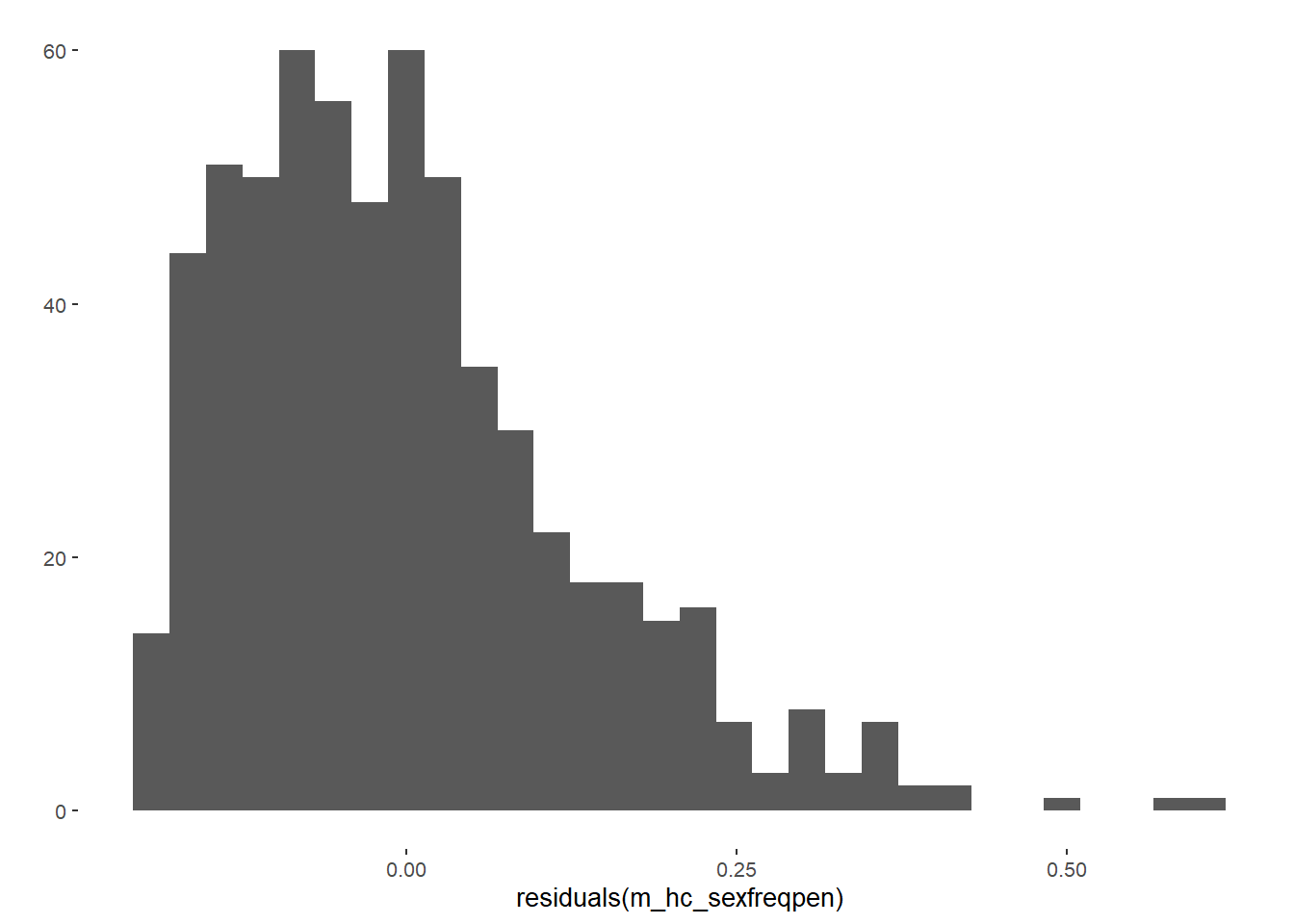
##
## Call:
## lm(formula = diary_sex_active_sex_mean ~ contraception_hormonal_numeric +
##     congruent_contraception_numeric + hc_con_interaction, data = data)
##
## Residuals:
##     Min      1Q  Median      3Q     Max
## -0.1971 -0.0982 -0.0240  0.0676  0.6029
##
## Coefficients:
##                                 Estimate Std. Error t value Pr(>|t|)
## (Intercept)                       0.1547     0.0118   13.07   <2e-16 ***
## contraception_hormonal_numeric    0.0279     0.0176    1.59     0.11
## congruent_contraception_numeric   0.0164     0.0150    1.09     0.27
## hc_con_interaction               -0.0019     0.0221   -0.09     0.93
## ---
## Signif. codes:  0 '***' 0.001 '**' 0.01 '*' 0.05 '.' 0.1 ' ' 1
##
## Residual standard error: 0.132 on 618 degrees of freedom
##   (557 Beobachtungen als fehlend gelöscht)
## Multiple R-squared:  0.0135, Adjusted R-squared:  0.00871
## F-statistic: 2.82 on 3 and 618 DF, p-value: 0.0383## # A tibble: 4 x 7
## term estimate std.error statistic p.value conf.low conf.high
## <chr> <dbl> <dbl> <dbl> <dbl> <dbl> <dbl>
## 1 (Intercept) 0.155 0.0118 13.1 1.23e-34 0.131 0.178
## 2 contraception_hormonal_numeric 0.0279 0.0176 1.59 1.13e- 1 -0.00666 0.0625
## 3 congruent_contraception_numeric 0.0164 0.0150 1.09 2.75e- 1 -0.0131 0.0458
## 4 hc_con_interaction -0.00190 0.0221 -0.0860 9.31e- 1 -0.0453 0.0415Sensitivity Analyses
HC
m_hc_sexfreqpen_sensitivity_hc <- sensemakr(model = m_hc_sexfreqpen,
                                         treatment = "contraception_hormonal_numeric",
                                        kd = 1:3, #these arguments parameterize how many times
                                          #stronger the confounder is related to the
                                          #treatment
                                ky = 1:3, #these arguments parameterize how many times
                                          #stronger the confounder is related to the outcome
                                q = 1, #fraction of the effect estimate that would have to be
                                       #explained away to be problematic. Setting q = 1,
                                       #means that a reduction of 100% of the current effect
                                       #estimate, that is, a true effect of zero, would be
                                       #deemed problematic.
                                alpha = 0.05,
                                reduce = TRUE #confounder reduce absolute effect size
                                )


m_hc_sexfreqpen_sensitivity_hc
## Sensitivity Analysis to Unobserved Confounding
##
## Model Formula: diary_sex_active_sex_mean ~ contraception_hormonal_numeric +
## congruent_contraception_numeric + hc_con_interaction
##
## Null hypothesis: q = 1 and reduce = TRUE
##
## Unadjusted Estimates of ' contraception_hormonal_numeric ':
## Coef. estimate: 0.028
## Standard Error: 0.018
## t-value: 1.586
##
## Sensitivity Statistics:
## Partial R2 of treatment with outcome: 0.004
## Robustness Value, q = 1 : 0.062
## Robustness Value, q = 1 alpha = 0.05 : 0
##
## For more information, check summary.## Sensitivity Analysis to Unobserved Confounding
##
## Model Formula: diary_sex_active_sex_mean ~ contraception_hormonal_numeric +
## congruent_contraception_numeric + hc_con_interaction
##
## Null hypothesis: q = 1 and reduce = TRUE
## -- This means we are considering biases that reduce the absolute value of the current estimate.
## -- The null hypothesis deemed problematic is H0:tau = 0
##
## Unadjusted Estimates of 'contraception_hormonal_numeric':
## Coef. estimate: 0.028
## Standard Error: 0.018
## t-value (H0:tau = 0): 1.586
##
## Sensitivity Statistics:
## Partial R2 of treatment with outcome: 0.004
## Robustness Value, q = 1: 0.062
## Robustness Value, q = 1, alpha = 0.05: 0
##
## Verbal interpretation of sensitivity statistics:
##
## -- Partial R2 of the treatment with the outcome: an extreme confounder (orthogonal to the covariates) that explains 100% of the residual variance of the outcome, would need to explain at least 0.4% of the residual variance of the treatment to fully account for the observed estimated effect.
##
## -- Robustness Value, q = 1: unobserved confounders (orthogonal to the covariates) that explain more than 6.2% of the residual variance of both the treatment and the outcome are strong enough to bring the point estimate to 0 (a bias of 100% of the original estimate). Conversely, unobserved confounders that do not explain more than 6.2% of the residual variance of both the treatment and the outcome are not strong enough to bring the point estimate to 0.
##
## -- Robustness Value, q = 1, alpha = 0.05: unobserved confounders (orthogonal to the covariates) that explain more than 0% of the residual variance of both the treatment and the outcome are strong enough to bring the estimate to a range where it is no longer 'statistically different' from 0 (a bias of 100% of the original estimate), at the significance level of alpha = 0.05. Conversely, unobserved confounders that do not explain more than 0% of the residual variance of both the treatment and the outcome are not strong enough to bring the estimate to a range where it is no longer 'statistically different' from 0, at the significance level of alpha = 0.05.Congruency
m_hc_sexfreqpen_sensitivity_con <- sensemakr(model = m_hc_sexfreqpen,
                                         treatment = "congruent_contraception_numeric",
                                        kd = 1:3, #these arguments parameterize how many times
                                          #stronger the confounder is related to the
                                          #treatment
                                ky = 1:3, #these arguments parameterize how many times
                                          #stronger the confounder is related to the outcome
                                q = 1, #fraction of the effect estimate that would have to be
                                       #explained away to be problematic. Setting q = 1,
                                       #means that a reduction of 100% of the current effect
                                       #estimate, that is, a true effect of zero, would be
                                       #deemed problematic.
                                alpha = 0.05,
                                reduce = TRUE #confounder reduce absolute effect size
                                )


m_hc_sexfreqpen_sensitivity_con
## Sensitivity Analysis to Unobserved Confounding
##
## Model Formula: diary_sex_active_sex_mean ~ contraception_hormonal_numeric +
## congruent_contraception_numeric + hc_con_interaction
##
## Null hypothesis: q = 1 and reduce = TRUE
##
## Unadjusted Estimates of ' congruent_contraception_numeric ':
## Coef. estimate: 0.016
## Standard Error: 0.015
## t-value: 1.093
##
## Sensitivity Statistics:
## Partial R2 of treatment with outcome: 0.002
## Robustness Value, q = 1 : 0.043
## Robustness Value, q = 1 alpha = 0.05 : 0
##
## For more information, check summary.## Sensitivity Analysis to Unobserved Confounding
##
## Model Formula: diary_sex_active_sex_mean ~ contraception_hormonal_numeric +
## congruent_contraception_numeric + hc_con_interaction
##
## Null hypothesis: q = 1 and reduce = TRUE
## -- This means we are considering biases that reduce the absolute value of the current estimate.
## -- The null hypothesis deemed problematic is H0:tau = 0
##
## Unadjusted Estimates of 'congruent_contraception_numeric':
## Coef. estimate: 0.016
## Standard Error: 0.015
## t-value (H0:tau = 0): 1.093
##
## Sensitivity Statistics:
## Partial R2 of treatment with outcome: 0.002
## Robustness Value, q = 1: 0.043
## Robustness Value, q = 1, alpha = 0.05: 0
##
## Verbal interpretation of sensitivity statistics:
##
## -- Partial R2 of the treatment with the outcome: an extreme confounder (orthogonal to the covariates) that explains 100% of the residual variance of the outcome, would need to explain at least 0.2% of the residual variance of the treatment to fully account for the observed estimated effect.
##
## -- Robustness Value, q = 1: unobserved confounders (orthogonal to the covariates) that explain more than 4.3% of the residual variance of both the treatment and the outcome are strong enough to bring the point estimate to 0 (a bias of 100% of the original estimate). Conversely, unobserved confounders that do not explain more than 4.3% of the residual variance of both the treatment and the outcome are not strong enough to bring the point estimate to 0.
##
## -- Robustness Value, q = 1, alpha = 0.05: unobserved confounders (orthogonal to the covariates) that explain more than 0% of the residual variance of both the treatment and the outcome are strong enough to bring the estimate to a range where it is no longer 'statistically different' from 0 (a bias of 100% of the original estimate), at the significance level of alpha = 0.05. Conversely, unobserved confounders that do not explain more than 0% of the residual variance of both the treatment and the outcome are not strong enough to bring the estimate to a range where it is no longer 'statistically different' from 0, at the significance level of alpha = 0.05.Interaction
m_hc_sexfreqpen_sensitivity_interaction <- sensemakr(model = m_hc_sexfreqpen,
                                         treatment = "hc_con_interaction",
                                        kd = 1:3, #these arguments parameterize how many times
                                          #stronger the confounder is related to the
                                          #treatment
                                ky = 1:3, #these arguments parameterize how many times
                                          #stronger the confounder is related to the outcome
                                q = 1, #fraction of the effect estimate that would have to be
                                       #explained away to be problematic. Setting q = 1,
                                       #means that a reduction of 100% of the current effect
                                       #estimate, that is, a true effect of zero, would be
                                       #deemed problematic.
                                alpha = 0.05,
                                reduce = TRUE #confounder reduce absolute effect size
                                )


m_hc_sexfreqpen_sensitivity_interaction
## Sensitivity Analysis to Unobserved Confounding
##
## Model Formula: diary_sex_active_sex_mean ~ contraception_hormonal_numeric +
## congruent_contraception_numeric + hc_con_interaction
##
## Null hypothesis: q = 1 and reduce = TRUE
##
## Unadjusted Estimates of ' hc_con_interaction ':
## Coef. estimate: -0.002
## Standard Error: 0.022
## t-value: -0.086
##
## Sensitivity Statistics:
## Partial R2 of treatment with outcome: 0
## Robustness Value, q = 1 : 0.003
## Robustness Value, q = 1 alpha = 0.05 : 0
##
## For more information, check summary.## Sensitivity Analysis to Unobserved Confounding
##
## Model Formula: diary_sex_active_sex_mean ~ contraception_hormonal_numeric +
## congruent_contraception_numeric + hc_con_interaction
##
## Null hypothesis: q = 1 and reduce = TRUE
## -- This means we are considering biases that reduce the absolute value of the current estimate.
## -- The null hypothesis deemed problematic is H0:tau = 0
##
## Unadjusted Estimates of 'hc_con_interaction':
## Coef. estimate: -0.002
## Standard Error: 0.022
## t-value (H0:tau = 0): -0.086
##
## Sensitivity Statistics:
## Partial R2 of treatment with outcome: 0
## Robustness Value, q = 1: 0.003
## Robustness Value, q = 1, alpha = 0.05: 0
##
## Verbal interpretation of sensitivity statistics:
##
## -- Partial R2 of the treatment with the outcome: an extreme confounder (orthogonal to the covariates) that explains 100% of the residual variance of the outcome, would need to explain at least 0% of the residual variance of the treatment to fully account for the observed estimated effect.
##
## -- Robustness Value, q = 1: unobserved confounders (orthogonal to the covariates) that explain more than 0.3% of the residual variance of both the treatment and the outcome are strong enough to bring the point estimate to 0 (a bias of 100% of the original estimate). Conversely, unobserved confounders that do not explain more than 0.3% of the residual variance of both the treatment and the outcome are not strong enough to bring the point estimate to 0.
##
## -- Robustness Value, q = 1, alpha = 0.05: unobserved confounders (orthogonal to the covariates) that explain more than 0% of the residual variance of both the treatment and the outcome are strong enough to bring the estimate to a range where it is no longer 'statistically different' from 0 (a bias of 100% of the original estimate), at the significance level of alpha = 0.05. Conversely, unobserved confounders that do not explain more than 0% of the residual variance of both the treatment and the outcome are not strong enough to bring the estimate to a range where it is no longer 'statistically different' from 0, at the significance level of alpha = 0.05.Controlled Model
Model
m_hc_sexfreqpen = lm(diary_sex_active_sex_mean ~ contraception_hormonal_numeric + congruent_contraception_numeric +
                         hc_con_interaction +
                       age + net_income + relationship_duration_factor +
                              education_years +
                              bfi_extra + bfi_neuro + bfi_agree + bfi_consc + bfi_open +
                              religiosity,
               data = data)
qplot(residuals(m_hc_sexfreqpen))
## `stat_bin()` using `bins = 30`. Pick better value with `binwidth`.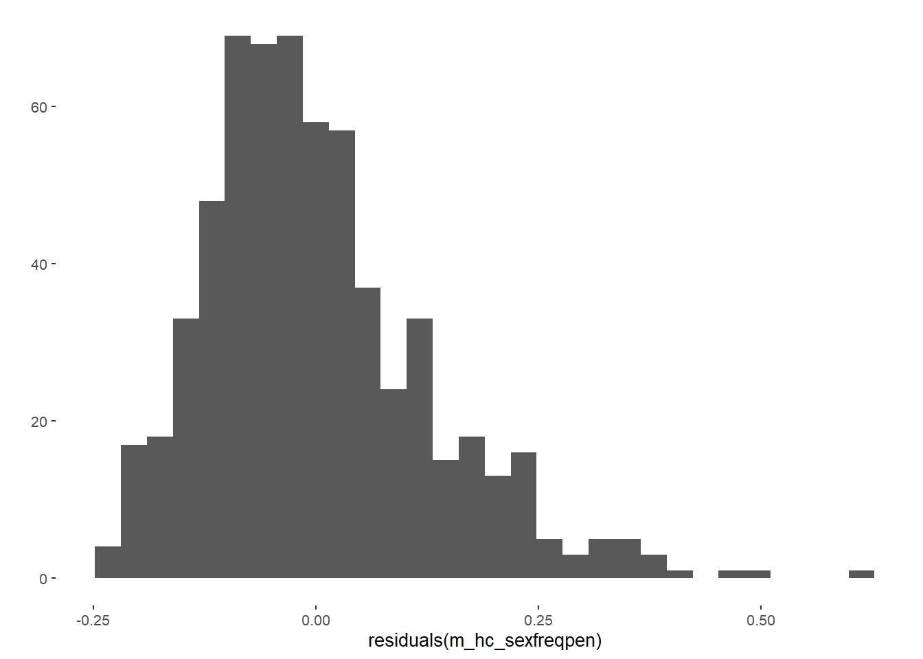
##
## Call:
## lm(formula = diary_sex_active_sex_mean ~ contraception_hormonal_numeric +
##     congruent_contraception_numeric + hc_con_interaction + age +
##     net_income + relationship_duration_factor + education_years +
##     bfi_extra + bfi_neuro + bfi_agree + bfi_consc + bfi_open +
##     religiosity, data = data)
##
## Residuals:
##     Min      1Q  Median      3Q     Max
## -0.2427 -0.0888 -0.0199  0.0636  0.6035
##
## Coefficients:
##                                                         Estimate Std. Error t value Pr(>|t|)
## (Intercept)                                             0.170500   0.073915    2.31   0.0214 *
## contraception_hormonal_numeric                          0.019092   0.017698    1.08   0.2811
## congruent_contraception_numeric                        -0.004746   0.015439   -0.31   0.7587
## hc_con_interaction                                      0.016155   0.022164    0.73   0.4664
## age                                                    -0.000856   0.001336   -0.64   0.5220
## net_incomeeuro_500_1000                                 0.027918   0.013333    2.09   0.0367 *
## net_incomeeuro_1000_2000                                0.024491   0.017657    1.39   0.1659
## net_incomeeuro_2000_3000                                0.065465   0.024764    2.64   0.0084 **
## net_incomeeuro_gt_3000                                  0.013700   0.042519    0.32   0.7474
## net_incomedont_tell                                     0.075390   0.033877    2.23   0.0264 *
## relationship_duration_factorPartnered_upto28months     -0.026559   0.014830   -1.79   0.0738 .
## relationship_duration_factorPartnered_upto52months     -0.067117   0.015998   -4.20 0.000031 ***
## relationship_duration_factorPartnered_morethan52months -0.066856   0.016464   -4.06 0.000055 ***
## education_years                                        -0.001859   0.001203   -1.55   0.1226
## bfi_extra                                              -0.000444   0.007280   -0.06   0.9514
## bfi_neuro                                              -0.000709   0.007851   -0.09   0.9281
## bfi_agree                                               0.016880   0.009055    1.86   0.0628 .
## bfi_consc                                              -0.005022   0.008152   -0.62   0.5381
## bfi_open                                                0.007581   0.008753    0.87   0.3868
## religiosity                                            -0.002599   0.003925   -0.66   0.5081
## ---
## Signif. codes:  0 '***' 0.001 '**' 0.01 '*' 0.05 '.' 0.1 ' ' 1
##
## Residual standard error: 0.129 on 602 degrees of freedom
##   (557 Beobachtungen als fehlend gelöscht)
## Multiple R-squared:  0.0905, Adjusted R-squared:  0.0618
## F-statistic: 3.15 on 19 and 602 DF, p-value: 0.00000819## # A tibble: 20 x 7
## term estimate std.error statistic p.value conf.low conf.high
## <chr> <dbl> <dbl> <dbl> <dbl> <dbl> <dbl>
## 1 (Intercept) 1.70e-1 0.0739 2.31 2.14e-2 2.53e-2 0.316
## 2 contraception_hormonal_numeric 1.91e-2 0.0177 1.08 2.81e-1 -1.57e-2 0.0538
## 3 congruent_contraception_numeric -4.75e-3 0.0154 -0.307 7.59e-1 -3.51e-2 0.0256
## 4 hc_con_interaction 1.62e-2 0.0222 0.729 4.66e-1 -2.74e-2 0.0597
## 5 age -8.56e-4 0.00134 -0.641 5.22e-1 -3.48e-3 0.00177
## 6 net_incomeeuro_500_1000 2.79e-2 0.0133 2.09 3.67e-2 1.73e-3 0.0541
## 7 net_incomeeuro_1000_2000 2.45e-2 0.0177 1.39 1.66e-1 -1.02e-2 0.0592
## 8 net_incomeeuro_2000_3000 6.55e-2 0.0248 2.64 8.42e-3 1.68e-2 0.114
## 9 net_incomeeuro_gt_3000 1.37e-2 0.0425 0.322 7.47e-1 -6.98e-2 0.0972
## 10 net_incomedont_tell 7.54e-2 0.0339 2.23 2.64e-2 8.86e-3 0.142
## 11 relationship_duration_factorPartnered_upto28months -2.66e-2 0.0148 -1.79 7.38e-2 -5.57e-2 0.00257
## 12 relationship_duration_factorPartnered_upto52months -6.71e-2 0.0160 -4.20 3.13e-5 -9.85e-2 -0.0357
## 13 relationship_duration_factorPartnered_morethan52months -6.69e-2 0.0165 -4.06 5.54e-5 -9.92e-2 -0.0345
## 14 education_years -1.86e-3 0.00120 -1.55 1.23e-1 -4.22e-3 0.000502
## 15 bfi_extra -4.44e-4 0.00728 -0.0609 9.51e-1 -1.47e-2 0.0139
## 16 bfi_neuro -7.09e-4 0.00785 -0.0903 9.28e-1 -1.61e-2 0.0147
## 17 bfi_agree 1.69e-2 0.00905 1.86 6.28e-2 -9.03e-4 0.0347
## 18 bfi_consc -5.02e-3 0.00815 -0.616 5.38e-1 -2.10e-2 0.0110
## 19 bfi_open 7.58e-3 0.00875 0.866 3.87e-1 -9.61e-3 0.0248
## 20 religiosity -2.60e-3 0.00393 -0.662 5.08e-1 -1.03e-2 0.00511Sensitivity Analyses
HC
m_hc_sexfreqpen_sensitivity_hc <- sensemakr(model = m_hc_sexfreqpen,
                                         treatment = "contraception_hormonal_numeric",
                                         benchmark_covariates = covariates, #covariates that will be
                                                                   #used to bound the
                                                                   #plausible strength of the
                                                                   #unobserved confounders
                                kd = 1:3, #these arguments parameterize how many times
                                          #stronger the confounder is related to the
                                          #treatment
                                ky = 1:3, #these arguments parameterize how many times
                                          #stronger the confounder is related to the outcome
                                q = 1, #fraction of the effect estimate that would have to be
                                       #explained away to be problematic. Setting q = 1,
                                       #means that a reduction of 100% of the current effect
                                       #estimate, that is, a true effect of zero, would be
                                       #deemed problematic.
                                alpha = 0.05,
                                reduce = TRUE #confounder reduce absolute effect size
                                )


m_hc_sexfreqpen_sensitivity_hc
## Sensitivity Analysis to Unobserved Confounding
##
## Model Formula: diary_sex_active_sex_mean ~ contraception_hormonal_numeric +
## congruent_contraception_numeric + hc_con_interaction + age +
## net_income + relationship_duration_factor + education_years +
## bfi_extra + bfi_neuro + bfi_agree + bfi_consc + bfi_open +
## religiosity
##
## Null hypothesis: q = 1 and reduce = TRUE
##
## Unadjusted Estimates of ' contraception_hormonal_numeric ':
## Coef. estimate: 0.019
## Standard Error: 0.018
## t-value: 1.079
##
## Sensitivity Statistics:
## Partial R2 of treatment with outcome: 0.002
## Robustness Value, q = 1 : 0.043
## Robustness Value, q = 1 alpha = 0.05 : 0
##
## For more information, check summary.## Sensitivity Analysis to Unobserved Confounding
##
## Model Formula: diary_sex_active_sex_mean ~ contraception_hormonal_numeric +
## congruent_contraception_numeric + hc_con_interaction + age +
## net_income + relationship_duration_factor + education_years +
## bfi_extra + bfi_neuro + bfi_agree + bfi_consc + bfi_open +
## religiosity
##
## Null hypothesis: q = 1 and reduce = TRUE
## -- This means we are considering biases that reduce the absolute value of the current estimate.
## -- The null hypothesis deemed problematic is H0:tau = 0
##
## Unadjusted Estimates of 'contraception_hormonal_numeric':
## Coef. estimate: 0.019
## Standard Error: 0.018
## t-value (H0:tau = 0): 1.079
##
## Sensitivity Statistics:
## Partial R2 of treatment with outcome: 0.002
## Robustness Value, q = 1: 0.043
## Robustness Value, q = 1, alpha = 0.05: 0
##
## Verbal interpretation of sensitivity statistics:
##
## -- Partial R2 of the treatment with the outcome: an extreme confounder (orthogonal to the covariates) that explains 100% of the residual variance of the outcome, would need to explain at least 0.2% of the residual variance of the treatment to fully account for the observed estimated effect.
##
## -- Robustness Value, q = 1: unobserved confounders (orthogonal to the covariates) that explain more than 4.3% of the residual variance of both the treatment and the outcome are strong enough to bring the point estimate to 0 (a bias of 100% of the original estimate). Conversely, unobserved confounders that do not explain more than 4.3% of the residual variance of both the treatment and the outcome are not strong enough to bring the point estimate to 0.
##
## -- Robustness Value, q = 1, alpha = 0.05: unobserved confounders (orthogonal to the covariates) that explain more than 0% of the residual variance of both the treatment and the outcome are strong enough to bring the estimate to a range where it is no longer 'statistically different' from 0 (a bias of 100% of the original estimate), at the significance level of alpha = 0.05. Conversely, unobserved confounders that do not explain more than 0% of the residual variance of both the treatment and the outcome are not strong enough to bring the estimate to a range where it is no longer 'statistically different' from 0, at the significance level of alpha = 0.05.
##
## Bounds on omitted variable bias:
##
## --The table below shows the maximum strength of unobserved confounders with association with the treatment and the outcome bounded by a multiple of the observed explanatory power of the chosen benchmark covariate(s).
##
## Bound Label R2dz.x R2yz.dx Treatment
## 1x age 0.025 0.001 contraception_hormonal_numeric
## 2x age 0.050 0.001 contraception_hormonal_numeric
## 3x age 0.076 0.002 contraception_hormonal_numeric
## 1x net_incomeeuro_500_1000 0.002 0.007 contraception_hormonal_numeric
## 2x net_incomeeuro_500_1000 0.003 0.015 contraception_hormonal_numeric
## 3x net_incomeeuro_500_1000 0.005 0.022 contraception_hormonal_numeric
## 1x net_incomeeuro_1000_2000 0.001 0.003 contraception_hormonal_numeric
## 2x net_incomeeuro_1000_2000 0.003 0.006 contraception_hormonal_numeric
## 3x net_incomeeuro_1000_2000 0.004 0.010 contraception_hormonal_numeric
## 1x net_incomeeuro_2000_3000 0.000 0.012 contraception_hormonal_numeric
## 2x net_incomeeuro_2000_3000 0.000 0.023 contraception_hormonal_numeric
## 3x net_incomeeuro_2000_3000 0.000 0.035 contraception_hormonal_numeric
## 1x net_incomeeuro_gt_3000 0.001 0.000 contraception_hormonal_numeric
## 2x net_incomeeuro_gt_3000 0.001 0.000 contraception_hormonal_numeric
## 3x net_incomeeuro_gt_3000 0.002 0.001 contraception_hormonal_numeric
## 1x net_incomedont_tell 0.001 0.008 contraception_hormonal_numeric
## 2x net_incomedont_tell 0.003 0.016 contraception_hormonal_numeric
## 3x net_incomedont_tell 0.004 0.025 contraception_hormonal_numeric
## 1x relationship_duration_factorPartnered_upto28months 0.001 0.005 contraception_hormonal_numeric
## 2x relationship_duration_factorPartnered_upto28months 0.002 0.011 contraception_hormonal_numeric
## 3x relationship_duration_factorPartnered_upto28months 0.003 0.016 contraception_hormonal_numeric
## 1x relationship_duration_factorPartnered_upto52months 0.002 0.029 contraception_hormonal_numeric
## 2x relationship_duration_factorPartnered_upto52months 0.003 0.059 contraception_hormonal_numeric
## 3x relationship_duration_factorPartnered_upto52months 0.005 0.088 contraception_hormonal_numeric
## 1x relationship_duration_factorPartnered_morethan52months 0.001 0.027 contraception_hormonal_numeric
## 2x relationship_duration_factorPartnered_morethan52months 0.003 0.055 contraception_hormonal_numeric
## 3x relationship_duration_factorPartnered_morethan52months 0.004 0.082 contraception_hormonal_numeric
## 1x education_years 0.011 0.004 contraception_hormonal_numeric
## 2x education_years 0.021 0.008 contraception_hormonal_numeric
## 3x education_years 0.032 0.012 contraception_hormonal_numeric
## 1x bfi_extra 0.000 0.000 contraception_hormonal_numeric
## 2x bfi_extra 0.000 0.000 contraception_hormonal_numeric
## 3x bfi_extra 0.000 0.000 contraception_hormonal_numeric
## 1x bfi_neuro 0.002 0.000 contraception_hormonal_numeric
## 2x bfi_neuro 0.004 0.000 contraception_hormonal_numeric
## 3x bfi_neuro 0.006 0.000 contraception_hormonal_numeric
## 1x bfi_agree 0.010 0.006 contraception_hormonal_numeric
## 2x bfi_agree 0.020 0.012 contraception_hormonal_numeric
## 3x bfi_agree 0.030 0.018 contraception_hormonal_numeric
## 1x bfi_consc 0.002 0.001 contraception_hormonal_numeric
## 2x bfi_consc 0.003 0.001 contraception_hormonal_numeric
## 3x bfi_consc 0.005 0.002 contraception_hormonal_numeric
## 1x bfi_open 0.001 0.001 contraception_hormonal_numeric
## 2x bfi_open 0.001 0.002 contraception_hormonal_numeric
## 3x bfi_open 0.002 0.004 contraception_hormonal_numeric
## 1x religiosity 0.002 0.001 contraception_hormonal_numeric
## 2x religiosity 0.005 0.001 contraception_hormonal_numeric
## 3x religiosity 0.007 0.002 contraception_hormonal_numeric
## Adjusted Estimate Adjusted Se Adjusted T Adjusted Lower CI Adjusted Upper CI
## 0.017 0.018 0.960 -0.018 0.052
## 0.015 0.018 0.842 -0.020 0.051
## 0.013 0.018 0.724 -0.023 0.049
## 0.018 0.018 0.999 -0.017 0.052
## 0.016 0.018 0.920 -0.018 0.051
## 0.015 0.018 0.840 -0.020 0.049
## 0.018 0.018 1.025 -0.017 0.053
## 0.017 0.018 0.972 -0.018 0.052
## 0.016 0.018 0.919 -0.018 0.051
## 0.019 0.018 1.079 -0.016 0.054
## 0.019 0.018 1.081 -0.015 0.053
## 0.019 0.017 1.083 -0.015 0.053
## 0.019 0.018 1.069 -0.016 0.054
## 0.019 0.018 1.060 -0.016 0.054
## 0.019 0.018 1.051 -0.016 0.053
## 0.018 0.018 1.000 -0.017 0.052
## 0.016 0.018 0.921 -0.018 0.051
## 0.015 0.018 0.842 -0.020 0.049
## 0.018 0.018 1.023 -0.017 0.053
## 0.017 0.018 0.968 -0.018 0.052
## 0.016 0.018 0.913 -0.018 0.051
## 0.016 0.017 0.924 -0.018 0.050
## 0.013 0.017 0.766 -0.021 0.047
## 0.010 0.017 0.602 -0.023 0.044
## 0.016 0.017 0.934 -0.018 0.051
## 0.014 0.017 0.785 -0.020 0.047
## 0.011 0.017 0.633 -0.023 0.044
## 0.016 0.018 0.914 -0.019 0.051
## 0.013 0.018 0.749 -0.022 0.048
## 0.010 0.018 0.583 -0.025 0.046
## 0.019 0.018 1.078 -0.016 0.054
## 0.019 0.018 1.077 -0.016 0.054
## 0.019 0.018 1.077 -0.016 0.054
## 0.019 0.018 1.073 -0.016 0.054
## 0.019 0.018 1.068 -0.016 0.054
## 0.019 0.018 1.062 -0.016 0.054
## 0.016 0.018 0.886 -0.019 0.051
## 0.012 0.018 0.694 -0.023 0.047
## 0.009 0.018 0.500 -0.026 0.044
## 0.019 0.018 1.052 -0.016 0.053
## 0.018 0.018 1.025 -0.017 0.053
## 0.018 0.018 0.999 -0.017 0.053
## 0.019 0.018 1.056 -0.016 0.053
## 0.018 0.018 1.033 -0.016 0.053
## 0.018 0.018 1.011 -0.017 0.053
## 0.019 0.018 1.044 -0.016 0.053
## 0.018 0.018 1.010 -0.017 0.053
## 0.017 0.018 0.975 -0.018 0.052Congreuncy
m_hc_sexfreqpen_sensitivity_con <- sensemakr(model = m_hc_sexfreqpen,
                                         treatment = "congruent_contraception_numeric",
                                         benchmark_covariates = covariates, #covariates that will be
                                                                   #used to bound the
                                                                   #plausible strength of the
                                                                   #unobserved confounders
                                kd = 1:3, #these arguments parameterize how many times
                                          #stronger the confounder is related to the
                                          #treatment
                                ky = 1:3, #these arguments parameterize how many times
                                          #stronger the confounder is related to the outcome
                                q = 1, #fraction of the effect estimate that would have to be
                                       #explained away to be problematic. Setting q = 1,
                                       #means that a reduction of 100% of the current effect
                                       #estimate, that is, a true effect of zero, would be
                                       #deemed problematic.
                                alpha = 0.05,
                                reduce = TRUE #confounder reduce absolute effect size
                                )


m_hc_sexfreqpen_sensitivity_con
## Sensitivity Analysis to Unobserved Confounding
##
## Model Formula: diary_sex_active_sex_mean ~ contraception_hormonal_numeric +
## congruent_contraception_numeric + hc_con_interaction + age +
## net_income + relationship_duration_factor + education_years +
## bfi_extra + bfi_neuro + bfi_agree + bfi_consc + bfi_open +
## religiosity
##
## Null hypothesis: q = 1 and reduce = TRUE
##
## Unadjusted Estimates of ' congruent_contraception_numeric ':
## Coef. estimate: -0.005
## Standard Error: 0.015
## t-value: -0.307
##
## Sensitivity Statistics:
## Partial R2 of treatment with outcome: 0
## Robustness Value, q = 1 : 0.012
## Robustness Value, q = 1 alpha = 0.05 : 0
##
## For more information, check summary.## Sensitivity Analysis to Unobserved Confounding
##
## Model Formula: diary_sex_active_sex_mean ~ contraception_hormonal_numeric +
## congruent_contraception_numeric + hc_con_interaction + age +
## net_income + relationship_duration_factor + education_years +
## bfi_extra + bfi_neuro + bfi_agree + bfi_consc + bfi_open +
## religiosity
##
## Null hypothesis: q = 1 and reduce = TRUE
## -- This means we are considering biases that reduce the absolute value of the current estimate.
## -- The null hypothesis deemed problematic is H0:tau = 0
##
## Unadjusted Estimates of 'congruent_contraception_numeric':
## Coef. estimate: -0.005
## Standard Error: 0.015
## t-value (H0:tau = 0): -0.307
##
## Sensitivity Statistics:
## Partial R2 of treatment with outcome: 0
## Robustness Value, q = 1: 0.012
## Robustness Value, q = 1, alpha = 0.05: 0
##
## Verbal interpretation of sensitivity statistics:
##
## -- Partial R2 of the treatment with the outcome: an extreme confounder (orthogonal to the covariates) that explains 100% of the residual variance of the outcome, would need to explain at least 0% of the residual variance of the treatment to fully account for the observed estimated effect.
##
## -- Robustness Value, q = 1: unobserved confounders (orthogonal to the covariates) that explain more than 1.2% of the residual variance of both the treatment and the outcome are strong enough to bring the point estimate to 0 (a bias of 100% of the original estimate). Conversely, unobserved confounders that do not explain more than 1.2% of the residual variance of both the treatment and the outcome are not strong enough to bring the point estimate to 0.
##
## -- Robustness Value, q = 1, alpha = 0.05: unobserved confounders (orthogonal to the covariates) that explain more than 0% of the residual variance of both the treatment and the outcome are strong enough to bring the estimate to a range where it is no longer 'statistically different' from 0 (a bias of 100% of the original estimate), at the significance level of alpha = 0.05. Conversely, unobserved confounders that do not explain more than 0% of the residual variance of both the treatment and the outcome are not strong enough to bring the estimate to a range where it is no longer 'statistically different' from 0, at the significance level of alpha = 0.05.
##
## Bounds on omitted variable bias:
##
## --The table below shows the maximum strength of unobserved confounders with association with the treatment and the outcome bounded by a multiple of the observed explanatory power of the chosen benchmark covariate(s).
##
## Bound Label R2dz.x R2yz.dx Treatment
## 1x age 0.003 0.001 congruent_contraception_numeric
## 2x age 0.006 0.001 congruent_contraception_numeric
## 3x age 0.009 0.002 congruent_contraception_numeric
## 1x net_incomeeuro_500_1000 0.001 0.007 congruent_contraception_numeric
## 2x net_incomeeuro_500_1000 0.001 0.015 congruent_contraception_numeric
## 3x net_incomeeuro_500_1000 0.002 0.022 congruent_contraception_numeric
## 1x net_incomeeuro_1000_2000 0.002 0.003 congruent_contraception_numeric
## 2x net_incomeeuro_1000_2000 0.004 0.006 congruent_contraception_numeric
## 3x net_incomeeuro_1000_2000 0.005 0.010 congruent_contraception_numeric
## 1x net_incomeeuro_2000_3000 0.005 0.012 congruent_contraception_numeric
## 2x net_incomeeuro_2000_3000 0.011 0.023 congruent_contraception_numeric
## 3x net_incomeeuro_2000_3000 0.016 0.035 congruent_contraception_numeric
## 1x net_incomeeuro_gt_3000 0.001 0.000 congruent_contraception_numeric
## 2x net_incomeeuro_gt_3000 0.002 0.000 congruent_contraception_numeric
## 3x net_incomeeuro_gt_3000 0.003 0.001 congruent_contraception_numeric
## 1x net_incomedont_tell 0.000 0.008 congruent_contraception_numeric
## 2x net_incomedont_tell 0.000 0.016 congruent_contraception_numeric
## 3x net_incomedont_tell 0.000 0.025 congruent_contraception_numeric
## 1x relationship_duration_factorPartnered_upto28months 0.016 0.006 congruent_contraception_numeric
## 2x relationship_duration_factorPartnered_upto28months 0.032 0.011 congruent_contraception_numeric
## 3x relationship_duration_factorPartnered_upto28months 0.048 0.017 congruent_contraception_numeric
## 1x relationship_duration_factorPartnered_upto52months 0.065 0.033 congruent_contraception_numeric
## 2x relationship_duration_factorPartnered_upto52months 0.131 0.067 congruent_contraception_numeric
## 3x relationship_duration_factorPartnered_upto52months 0.196 0.102 congruent_contraception_numeric
## 1x relationship_duration_factorPartnered_morethan52months 0.080 0.032 congruent_contraception_numeric
## 2x relationship_duration_factorPartnered_morethan52months 0.161 0.065 congruent_contraception_numeric
## 3x relationship_duration_factorPartnered_morethan52months 0.241 0.100 congruent_contraception_numeric
## 1x education_years 0.012 0.004 congruent_contraception_numeric
## 2x education_years 0.023 0.008 congruent_contraception_numeric
## 3x education_years 0.035 0.012 congruent_contraception_numeric
## 1x bfi_extra 0.000 0.000 congruent_contraception_numeric
## 2x bfi_extra 0.000 0.000 congruent_contraception_numeric
## 3x bfi_extra 0.000 0.000 congruent_contraception_numeric
## 1x bfi_neuro 0.003 0.000 congruent_contraception_numeric
## 2x bfi_neuro 0.005 0.000 congruent_contraception_numeric
## 3x bfi_neuro 0.008 0.000 congruent_contraception_numeric
## 1x bfi_agree 0.002 0.006 congruent_contraception_numeric
## 2x bfi_agree 0.003 0.012 congruent_contraception_numeric
## 3x bfi_agree 0.005 0.017 congruent_contraception_numeric
## 1x bfi_consc 0.000 0.001 congruent_contraception_numeric
## 2x bfi_consc 0.000 0.001 congruent_contraception_numeric
## 3x bfi_consc 0.001 0.002 congruent_contraception_numeric
## 1x bfi_open 0.001 0.001 congruent_contraception_numeric
## 2x bfi_open 0.001 0.002 congruent_contraception_numeric
## 3x bfi_open 0.002 0.004 congruent_contraception_numeric
## 1x religiosity 0.001 0.001 congruent_contraception_numeric
## 2x religiosity 0.002 0.001 congruent_contraception_numeric
## 3x religiosity 0.003 0.002 congruent_contraception_numeric
## Adjusted Estimate Adjusted Se Adjusted T Adjusted Lower CI Adjusted Upper CI
## -0.004 0.015 -0.271 -0.035 0.026
## -0.004 0.015 -0.235 -0.034 0.027
## -0.003 0.016 -0.199 -0.034 0.027
## -0.004 0.015 -0.257 -0.034 0.026
## -0.003 0.015 -0.206 -0.033 0.027
## -0.002 0.015 -0.155 -0.032 0.028
## -0.004 0.015 -0.248 -0.034 0.026
## -0.003 0.015 -0.188 -0.033 0.027
## -0.002 0.015 -0.129 -0.032 0.028
## -0.002 0.015 -0.112 -0.032 0.029
## 0.001 0.015 0.085 -0.029 0.031
## 0.004 0.015 0.285 -0.026 0.034
## -0.005 0.015 -0.297 -0.035 0.026
## -0.004 0.015 -0.286 -0.035 0.026
## -0.004 0.015 -0.276 -0.035 0.026
## -0.005 0.015 -0.298 -0.035 0.026
## -0.004 0.015 -0.289 -0.035 0.026
## -0.004 0.015 -0.279 -0.034 0.026
## -0.001 0.016 -0.074 -0.032 0.029
## 0.003 0.016 0.161 -0.028 0.033
## 0.006 0.016 0.397 -0.025 0.037
## 0.014 0.016 0.862 -0.017 0.044
## 0.033 0.016 2.085 0.002 0.065
## 0.055 0.016 3.369 0.023 0.087
## 0.015 0.016 0.968 -0.016 0.046
## 0.038 0.016 2.307 0.006 0.070
## 0.063 0.017 3.721 0.030 0.096
## -0.002 0.016 -0.136 -0.033 0.028
## 0.001 0.016 0.035 -0.030 0.031
## 0.003 0.016 0.208 -0.027 0.034
## -0.005 0.015 -0.307 -0.035 0.026
## -0.005 0.015 -0.307 -0.035 0.026
## -0.005 0.015 -0.307 -0.035 0.026
## -0.005 0.015 -0.302 -0.035 0.026
## -0.005 0.015 -0.297 -0.035 0.026
## -0.005 0.016 -0.292 -0.035 0.026
## -0.004 0.015 -0.232 -0.034 0.027
## -0.002 0.015 -0.156 -0.033 0.028
## -0.001 0.015 -0.080 -0.031 0.029
## -0.005 0.015 -0.298 -0.035 0.026
## -0.004 0.015 -0.288 -0.035 0.026
## -0.004 0.015 -0.279 -0.035 0.026
## -0.004 0.015 -0.287 -0.035 0.026
## -0.004 0.015 -0.268 -0.034 0.026
## -0.004 0.015 -0.248 -0.034 0.026
## -0.004 0.015 -0.286 -0.035 0.026
## -0.004 0.015 -0.265 -0.034 0.026
## -0.004 0.015 -0.244 -0.034 0.027Interaction
m_hc_sexfreqpen_sensitivity_interaction <- sensemakr(model = m_hc_sexfreqpen,
                                         treatment = "hc_con_interaction",
                                         benchmark_covariates = covariates, #covariates that will be
                                                                   #used to bound the
                                                                   #plausible strength of the
                                                                   #unobserved confounders
                                kd = 1:3, #these arguments parameterize how many times
                                          #stronger the confounder is related to the
                                          #treatment
                                ky = 1:3, #these arguments parameterize how many times
                                          #stronger the confounder is related to the outcome
                                q = 1, #fraction of the effect estimate that would have to be
                                       #explained away to be problematic. Setting q = 1,
                                       #means that a reduction of 100% of the current effect
                                       #estimate, that is, a true effect of zero, would be
                                       #deemed problematic.
                                alpha = 0.05,
                                reduce = TRUE #confounder reduce absolute effect size
                                )


m_hc_sexfreqpen_sensitivity_interaction
## Sensitivity Analysis to Unobserved Confounding
##
## Model Formula: diary_sex_active_sex_mean ~ contraception_hormonal_numeric +
## congruent_contraception_numeric + hc_con_interaction + age +
## net_income + relationship_duration_factor + education_years +
## bfi_extra + bfi_neuro + bfi_agree + bfi_consc + bfi_open +
## religiosity
##
## Null hypothesis: q = 1 and reduce = TRUE
##
## Unadjusted Estimates of ' hc_con_interaction ':
## Coef. estimate: 0.016
## Standard Error: 0.022
## t-value: 0.729
##
## Sensitivity Statistics:
## Partial R2 of treatment with outcome: 0.001
## Robustness Value, q = 1 : 0.029
## Robustness Value, q = 1 alpha = 0.05 : 0
##
## For more information, check summary.## Sensitivity Analysis to Unobserved Confounding
##
## Model Formula: diary_sex_active_sex_mean ~ contraception_hormonal_numeric +
## congruent_contraception_numeric + hc_con_interaction + age +
## net_income + relationship_duration_factor + education_years +
## bfi_extra + bfi_neuro + bfi_agree + bfi_consc + bfi_open +
## religiosity
##
## Null hypothesis: q = 1 and reduce = TRUE
## -- This means we are considering biases that reduce the absolute value of the current estimate.
## -- The null hypothesis deemed problematic is H0:tau = 0
##
## Unadjusted Estimates of 'hc_con_interaction':
## Coef. estimate: 0.016
## Standard Error: 0.022
## t-value (H0:tau = 0): 0.729
##
## Sensitivity Statistics:
## Partial R2 of treatment with outcome: 0.001
## Robustness Value, q = 1: 0.029
## Robustness Value, q = 1, alpha = 0.05: 0
##
## Verbal interpretation of sensitivity statistics:
##
## -- Partial R2 of the treatment with the outcome: an extreme confounder (orthogonal to the covariates) that explains 100% of the residual variance of the outcome, would need to explain at least 0.1% of the residual variance of the treatment to fully account for the observed estimated effect.
##
## -- Robustness Value, q = 1: unobserved confounders (orthogonal to the covariates) that explain more than 2.9% of the residual variance of both the treatment and the outcome are strong enough to bring the point estimate to 0 (a bias of 100% of the original estimate). Conversely, unobserved confounders that do not explain more than 2.9% of the residual variance of both the treatment and the outcome are not strong enough to bring the point estimate to 0.
##
## -- Robustness Value, q = 1, alpha = 0.05: unobserved confounders (orthogonal to the covariates) that explain more than 0% of the residual variance of both the treatment and the outcome are strong enough to bring the estimate to a range where it is no longer 'statistically different' from 0 (a bias of 100% of the original estimate), at the significance level of alpha = 0.05. Conversely, unobserved confounders that do not explain more than 0% of the residual variance of both the treatment and the outcome are not strong enough to bring the estimate to a range where it is no longer 'statistically different' from 0, at the significance level of alpha = 0.05.
##
## Bounds on omitted variable bias:
##
## --The table below shows the maximum strength of unobserved confounders with association with the treatment and the outcome bounded by a multiple of the observed explanatory power of the chosen benchmark covariate(s).
##
## Bound Label R2dz.x R2yz.dx Treatment
## 1x age 0.000 0.001 hc_con_interaction
## 2x age 0.001 0.001 hc_con_interaction
## 3x age 0.001 0.002 hc_con_interaction
## 1x net_incomeeuro_500_1000 0.000 0.007 hc_con_interaction
## 2x net_incomeeuro_500_1000 0.000 0.015 hc_con_interaction
## 3x net_incomeeuro_500_1000 0.001 0.022 hc_con_interaction
## 1x net_incomeeuro_1000_2000 0.002 0.003 hc_con_interaction
## 2x net_incomeeuro_1000_2000 0.004 0.006 hc_con_interaction
## 3x net_incomeeuro_1000_2000 0.006 0.010 hc_con_interaction
## 1x net_incomeeuro_2000_3000 0.000 0.012 hc_con_interaction
## 2x net_incomeeuro_2000_3000 0.001 0.023 hc_con_interaction
## 3x net_incomeeuro_2000_3000 0.001 0.035 hc_con_interaction
## 1x net_incomeeuro_gt_3000 0.000 0.000 hc_con_interaction
## 2x net_incomeeuro_gt_3000 0.000 0.000 hc_con_interaction
## 3x net_incomeeuro_gt_3000 0.000 0.001 hc_con_interaction
## 1x net_incomedont_tell 0.002 0.008 hc_con_interaction
## 2x net_incomedont_tell 0.004 0.017 hc_con_interaction
## 3x net_incomedont_tell 0.005 0.025 hc_con_interaction
## 1x relationship_duration_factorPartnered_upto28months 0.006 0.005 hc_con_interaction
## 2x relationship_duration_factorPartnered_upto28months 0.012 0.011 hc_con_interaction
## 3x relationship_duration_factorPartnered_upto28months 0.017 0.016 hc_con_interaction
## 1x relationship_duration_factorPartnered_upto52months 0.009 0.030 hc_con_interaction
## 2x relationship_duration_factorPartnered_upto52months 0.018 0.060 hc_con_interaction
## 3x relationship_duration_factorPartnered_upto52months 0.027 0.089 hc_con_interaction
## 1x relationship_duration_factorPartnered_morethan52months 0.019 0.028 hc_con_interaction
## 2x relationship_duration_factorPartnered_morethan52months 0.037 0.057 hc_con_interaction
## 3x relationship_duration_factorPartnered_morethan52months 0.056 0.085 hc_con_interaction
## 1x education_years 0.015 0.004 hc_con_interaction
## 2x education_years 0.029 0.008 hc_con_interaction
## 3x education_years 0.044 0.012 hc_con_interaction
## 1x bfi_extra 0.000 0.000 hc_con_interaction
## 2x bfi_extra 0.000 0.000 hc_con_interaction
## 3x bfi_extra 0.001 0.000 hc_con_interaction
## 1x bfi_neuro 0.001 0.000 hc_con_interaction
## 2x bfi_neuro 0.002 0.000 hc_con_interaction
## 3x bfi_neuro 0.004 0.000 hc_con_interaction
## 1x bfi_agree 0.006 0.006 hc_con_interaction
## 2x bfi_agree 0.012 0.012 hc_con_interaction
## 3x bfi_agree 0.019 0.018 hc_con_interaction
## 1x bfi_consc 0.001 0.001 hc_con_interaction
## 2x bfi_consc 0.003 0.001 hc_con_interaction
## 3x bfi_consc 0.004 0.002 hc_con_interaction
## 1x bfi_open 0.004 0.001 hc_con_interaction
## 2x bfi_open 0.008 0.003 hc_con_interaction
## 3x bfi_open 0.012 0.004 hc_con_interaction
## 1x religiosity 0.006 0.001 hc_con_interaction
## 2x religiosity 0.012 0.001 hc_con_interaction
## 3x religiosity 0.018 0.002 hc_con_interaction
## Adjusted Estimate Adjusted Se Adjusted T Adjusted Lower CI Adjusted Upper CI
## 0.016 0.022 0.717 -0.028 0.059
## 0.016 0.022 0.705 -0.028 0.059
## 0.015 0.022 0.694 -0.028 0.059
## 0.016 0.022 0.703 -0.028 0.059
## 0.015 0.022 0.678 -0.028 0.058
## 0.014 0.022 0.652 -0.029 0.057
## 0.015 0.022 0.665 -0.029 0.058
## 0.013 0.022 0.602 -0.030 0.057
## 0.012 0.022 0.538 -0.032 0.055
## 0.015 0.022 0.681 -0.028 0.058
## 0.014 0.022 0.632 -0.029 0.057
## 0.013 0.022 0.583 -0.030 0.056
## 0.016 0.022 0.726 -0.027 0.060
## 0.016 0.022 0.724 -0.027 0.060
## 0.016 0.022 0.722 -0.028 0.060
## 0.014 0.022 0.636 -0.029 0.057
## 0.012 0.022 0.543 -0.031 0.055
## 0.010 0.022 0.449 -0.033 0.053
## 0.013 0.022 0.591 -0.030 0.057
## 0.010 0.022 0.452 -0.034 0.054
## 0.007 0.022 0.313 -0.037 0.051
## 0.007 0.022 0.329 -0.036 0.050
## -0.002 0.022 -0.083 -0.044 0.041
## -0.011 0.021 -0.509 -0.053 0.031
## 0.004 0.022 0.159 -0.040 0.047
## -0.009 0.022 -0.428 -0.053 0.034
## -0.023 0.022 -1.033 -0.065 0.020
## 0.012 0.022 0.534 -0.032 0.056
## 0.008 0.022 0.339 -0.036 0.052
## 0.003 0.023 0.144 -0.041 0.048
## 0.016 0.022 0.727 -0.027 0.060
## 0.016 0.022 0.726 -0.027 0.060
## 0.016 0.022 0.725 -0.027 0.060
## 0.016 0.022 0.725 -0.028 0.060
## 0.016 0.022 0.721 -0.028 0.060
## 0.016 0.022 0.718 -0.028 0.060
## 0.013 0.022 0.580 -0.031 0.056
## 0.010 0.022 0.430 -0.034 0.053
## 0.006 0.022 0.280 -0.037 0.050
## 0.016 0.022 0.705 -0.028 0.059
## 0.015 0.022 0.682 -0.028 0.059
## 0.015 0.022 0.658 -0.029 0.058
## 0.015 0.022 0.672 -0.029 0.059
## 0.014 0.022 0.616 -0.030 0.057
## 0.012 0.022 0.559 -0.031 0.056
## 0.015 0.022 0.675 -0.029 0.059
## 0.014 0.022 0.622 -0.030 0.058
## 0.013 0.022 0.569 -0.031 0.057Masturbation Frequency
Uncontrolled Model
Model
m_hc_masfreq = lm(diary_masturbation_mean ~ contraception_hormonal_numeric + congruent_contraception_numeric +
                       hc_con_interaction,
                     data = data)
qplot(residuals(m_hc_masfreq))
## `stat_bin()` using `bins = 30`. Pick better value with `binwidth`.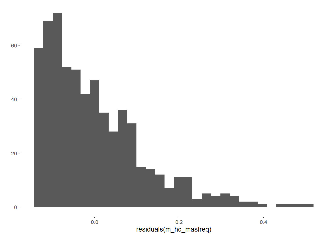
##
## Call:
## lm(formula = diary_masturbation_mean ~ contraception_hormonal_numeric +
##     congruent_contraception_numeric + hc_con_interaction, data = data)
##
## Residuals:
##     Min      1Q  Median      3Q     Max
## -0.1375 -0.0875 -0.0281  0.0601  0.5025
##
## Coefficients:
##                                 Estimate Std. Error t value Pr(>|t|)
## (Intercept)                      0.13038    0.01047   12.45   <2e-16 ***
## contraception_hormonal_numeric  -0.04286    0.01558   -2.75   0.0061 **
## congruent_contraception_numeric  0.00708    0.01326    0.53   0.5935
## hc_con_interaction               0.00691    0.01955    0.35   0.7239
## ---
## Signif. codes:  0 '***' 0.001 '**' 0.01 '*' 0.05 '.' 0.1 ' ' 1
##
## Residual standard error: 0.117 on 618 degrees of freedom
##   (557 Beobachtungen als fehlend gelöscht)
## Multiple R-squared:  0.0279, Adjusted R-squared:  0.0232
## F-statistic: 5.92 on 3 and 618 DF, p-value: 0.000552## # A tibble: 4 x 7
## term estimate std.error statistic p.value conf.low conf.high
## <chr> <dbl> <dbl> <dbl> <dbl> <dbl> <dbl>
## 1 (Intercept) 0.130 0.0105 12.4 6.62e-32 0.110 0.151
## 2 contraception_hormonal_numeric -0.0429 0.0156 -2.75 6.12e- 3 -0.0735 -0.0123
## 3 congruent_contraception_numeric 0.00708 0.0133 0.534 5.93e- 1 -0.0190 0.0331
## 4 hc_con_interaction 0.00691 0.0196 0.353 7.24e- 1 -0.0315 0.0453Sensitivity Analyses
HC
m_hc_masfreq_sensitivity_hc <- sensemakr(model = m_hc_masfreq,
                                            treatment = "contraception_hormonal_numeric",
                                            kd = 1:3, #these arguments parameterize how many times
                                            #stronger the confounder is related to the
                                            #treatment
                                            ky = 1:3, #these arguments parameterize how many times
                                            #stronger the confounder is related to the outcome
                                            q = 1, #fraction of the effect estimate that would have to be
                                            #explained away to be problematic. Setting q = 1,
                                            #means that a reduction of 100% of the current effect
                                            #estimate, that is, a true effect of zero, would be
                                            #deemed problematic.
                                            alpha = 0.05,
                                            reduce = TRUE #confounder reduce absolute effect size
)


m_hc_masfreq_sensitivity_hc
## Sensitivity Analysis to Unobserved Confounding
##
## Model Formula: diary_masturbation_mean ~ contraception_hormonal_numeric + congruent_contraception_numeric +
## hc_con_interaction
##
## Null hypothesis: q = 1 and reduce = TRUE
##
## Unadjusted Estimates of ' contraception_hormonal_numeric ':
## Coef. estimate: -0.043
## Standard Error: 0.016
## t-value: -2.751
##
## Sensitivity Statistics:
## Partial R2 of treatment with outcome: 0.012
## Robustness Value, q = 1 : 0.105
## Robustness Value, q = 1 alpha = 0.05 : 0.031
##
## For more information, check summary.## Sensitivity Analysis to Unobserved Confounding
##
## Model Formula: diary_masturbation_mean ~ contraception_hormonal_numeric + congruent_contraception_numeric +
## hc_con_interaction
##
## Null hypothesis: q = 1 and reduce = TRUE
## -- This means we are considering biases that reduce the absolute value of the current estimate.
## -- The null hypothesis deemed problematic is H0:tau = 0
##
## Unadjusted Estimates of 'contraception_hormonal_numeric':
## Coef. estimate: -0.043
## Standard Error: 0.016
## t-value (H0:tau = 0): -2.751
##
## Sensitivity Statistics:
## Partial R2 of treatment with outcome: 0.012
## Robustness Value, q = 1: 0.105
## Robustness Value, q = 1, alpha = 0.05: 0.031
##
## Verbal interpretation of sensitivity statistics:
##
## -- Partial R2 of the treatment with the outcome: an extreme confounder (orthogonal to the covariates) that explains 100% of the residual variance of the outcome, would need to explain at least 1.2% of the residual variance of the treatment to fully account for the observed estimated effect.
##
## -- Robustness Value, q = 1: unobserved confounders (orthogonal to the covariates) that explain more than 10.5% of the residual variance of both the treatment and the outcome are strong enough to bring the point estimate to 0 (a bias of 100% of the original estimate). Conversely, unobserved confounders that do not explain more than 10.5% of the residual variance of both the treatment and the outcome are not strong enough to bring the point estimate to 0.
##
## -- Robustness Value, q = 1, alpha = 0.05: unobserved confounders (orthogonal to the covariates) that explain more than 3.1% of the residual variance of both the treatment and the outcome are strong enough to bring the estimate to a range where it is no longer 'statistically different' from 0 (a bias of 100% of the original estimate), at the significance level of alpha = 0.05. Conversely, unobserved confounders that do not explain more than 3.1% of the residual variance of both the treatment and the outcome are not strong enough to bring the estimate to a range where it is no longer 'statistically different' from 0, at the significance level of alpha = 0.05.Congruency
m_hc_masfreq_sensitivity_con <- sensemakr(model = m_hc_masfreq,
treatment = "congruent_contraception_numeric",
kd = 1:3, #these arguments parameterize how many times
#stronger the confounder is related to the
#treatment
ky = 1:3, #these arguments parameterize how many times
#stronger the confounder is related to the outcome
q = 1, #fraction of the effect estimate that would have to be
#explained away to be problematic. Setting q = 1,
#means that a reduction of 100% of the current effect
#estimate, that is, a true effect of zero, would be
#deemed problematic.
alpha = 0.05,
reduce = TRUE #confounder reduce absolute effect size
)
m_hc_masfreq_sensitivity_con## Sensitivity Analysis to Unobserved Confounding
##
## Model Formula: diary_masturbation_mean ~ contraception_hormonal_numeric + congruent_contraception_numeric +
## hc_con_interaction
##
## Null hypothesis: q = 1 and reduce = TRUE
##
## Unadjusted Estimates of ' congruent_contraception_numeric ':
## Coef. estimate: 0.007
## Standard Error: 0.013
## t-value: 0.534
##
## Sensitivity Statistics:
## Partial R2 of treatment with outcome: 0
## Robustness Value, q = 1 : 0.021
## Robustness Value, q = 1 alpha = 0.05 : 0
##
## For more information, check summary.## Sensitivity Analysis to Unobserved Confounding
##
## Model Formula: diary_masturbation_mean ~ contraception_hormonal_numeric + congruent_contraception_numeric +
## hc_con_interaction
##
## Null hypothesis: q = 1 and reduce = TRUE
## -- This means we are considering biases that reduce the absolute value of the current estimate.
## -- The null hypothesis deemed problematic is H0:tau = 0
##
## Unadjusted Estimates of 'congruent_contraception_numeric':
## Coef. estimate: 0.007
## Standard Error: 0.013
## t-value (H0:tau = 0): 0.534
##
## Sensitivity Statistics:
## Partial R2 of treatment with outcome: 0
## Robustness Value, q = 1: 0.021
## Robustness Value, q = 1, alpha = 0.05: 0
##
## Verbal interpretation of sensitivity statistics:
##
## -- Partial R2 of the treatment with the outcome: an extreme confounder (orthogonal to the covariates) that explains 100% of the residual variance of the outcome, would need to explain at least 0% of the residual variance of the treatment to fully account for the observed estimated effect.
##
## -- Robustness Value, q = 1: unobserved confounders (orthogonal to the covariates) that explain more than 2.1% of the residual variance of both the treatment and the outcome are strong enough to bring the point estimate to 0 (a bias of 100% of the original estimate). Conversely, unobserved confounders that do not explain more than 2.1% of the residual variance of both the treatment and the outcome are not strong enough to bring the point estimate to 0.
##
## -- Robustness Value, q = 1, alpha = 0.05: unobserved confounders (orthogonal to the covariates) that explain more than 0% of the residual variance of both the treatment and the outcome are strong enough to bring the estimate to a range where it is no longer 'statistically different' from 0 (a bias of 100% of the original estimate), at the significance level of alpha = 0.05. Conversely, unobserved confounders that do not explain more than 0% of the residual variance of both the treatment and the outcome are not strong enough to bring the estimate to a range where it is no longer 'statistically different' from 0, at the significance level of alpha = 0.05.Interaction
m_hc_masfreq_sensitivity_interaction <- sensemakr(model = m_hc_masfreq,
treatment = "hc_con_interaction",
kd = 1:3, #these arguments parameterize how many times
#stronger the confounder is related to the
#treatment
ky = 1:3, #these arguments parameterize how many times
#stronger the confounder is related to the outcome
q = 1, #fraction of the effect estimate that would have to be
#explained away to be problematic. Setting q = 1,
#means that a reduction of 100% of the current effect
#estimate, that is, a true effect of zero, would be
#deemed problematic.
alpha = 0.05,
reduce = TRUE #confounder reduce absolute effect size
)
m_hc_masfreq_sensitivity_interaction## Sensitivity Analysis to Unobserved Confounding
##
## Model Formula: diary_masturbation_mean ~ contraception_hormonal_numeric + congruent_contraception_numeric +
## hc_con_interaction
##
## Null hypothesis: q = 1 and reduce = TRUE
##
## Unadjusted Estimates of ' hc_con_interaction ':
## Coef. estimate: 0.007
## Standard Error: 0.02
## t-value: 0.353
##
## Sensitivity Statistics:
## Partial R2 of treatment with outcome: 0
## Robustness Value, q = 1 : 0.014
## Robustness Value, q = 1 alpha = 0.05 : 0
##
## For more information, check summary.## Sensitivity Analysis to Unobserved Confounding
##
## Model Formula: diary_masturbation_mean ~ contraception_hormonal_numeric + congruent_contraception_numeric +
## hc_con_interaction
##
## Null hypothesis: q = 1 and reduce = TRUE
## -- This means we are considering biases that reduce the absolute value of the current estimate.
## -- The null hypothesis deemed problematic is H0:tau = 0
##
## Unadjusted Estimates of 'hc_con_interaction':
## Coef. estimate: 0.007
## Standard Error: 0.02
## t-value (H0:tau = 0): 0.353
##
## Sensitivity Statistics:
## Partial R2 of treatment with outcome: 0
## Robustness Value, q = 1: 0.014
## Robustness Value, q = 1, alpha = 0.05: 0
##
## Verbal interpretation of sensitivity statistics:
##
## -- Partial R2 of the treatment with the outcome: an extreme confounder (orthogonal to the covariates) that explains 100% of the residual variance of the outcome, would need to explain at least 0% of the residual variance of the treatment to fully account for the observed estimated effect.
##
## -- Robustness Value, q = 1: unobserved confounders (orthogonal to the covariates) that explain more than 1.4% of the residual variance of both the treatment and the outcome are strong enough to bring the point estimate to 0 (a bias of 100% of the original estimate). Conversely, unobserved confounders that do not explain more than 1.4% of the residual variance of both the treatment and the outcome are not strong enough to bring the point estimate to 0.
##
## -- Robustness Value, q = 1, alpha = 0.05: unobserved confounders (orthogonal to the covariates) that explain more than 0% of the residual variance of both the treatment and the outcome are strong enough to bring the estimate to a range where it is no longer 'statistically different' from 0 (a bias of 100% of the original estimate), at the significance level of alpha = 0.05. Conversely, unobserved confounders that do not explain more than 0% of the residual variance of both the treatment and the outcome are not strong enough to bring the estimate to a range where it is no longer 'statistically different' from 0, at the significance level of alpha = 0.05.Controlled Model
Model
m_hc_masfreq = lm(diary_masturbation_mean ~ contraception_hormonal_numeric + congruent_contraception_numeric +
hc_con_interaction +
age + net_income + relationship_duration_factor +
education_years +
bfi_extra + bfi_neuro + bfi_agree + bfi_consc + bfi_open +
religiosity,
data = data)
qplot(residuals(m_hc_masfreq))## `stat_bin()` using `bins = 30`. Pick better value with `binwidth`.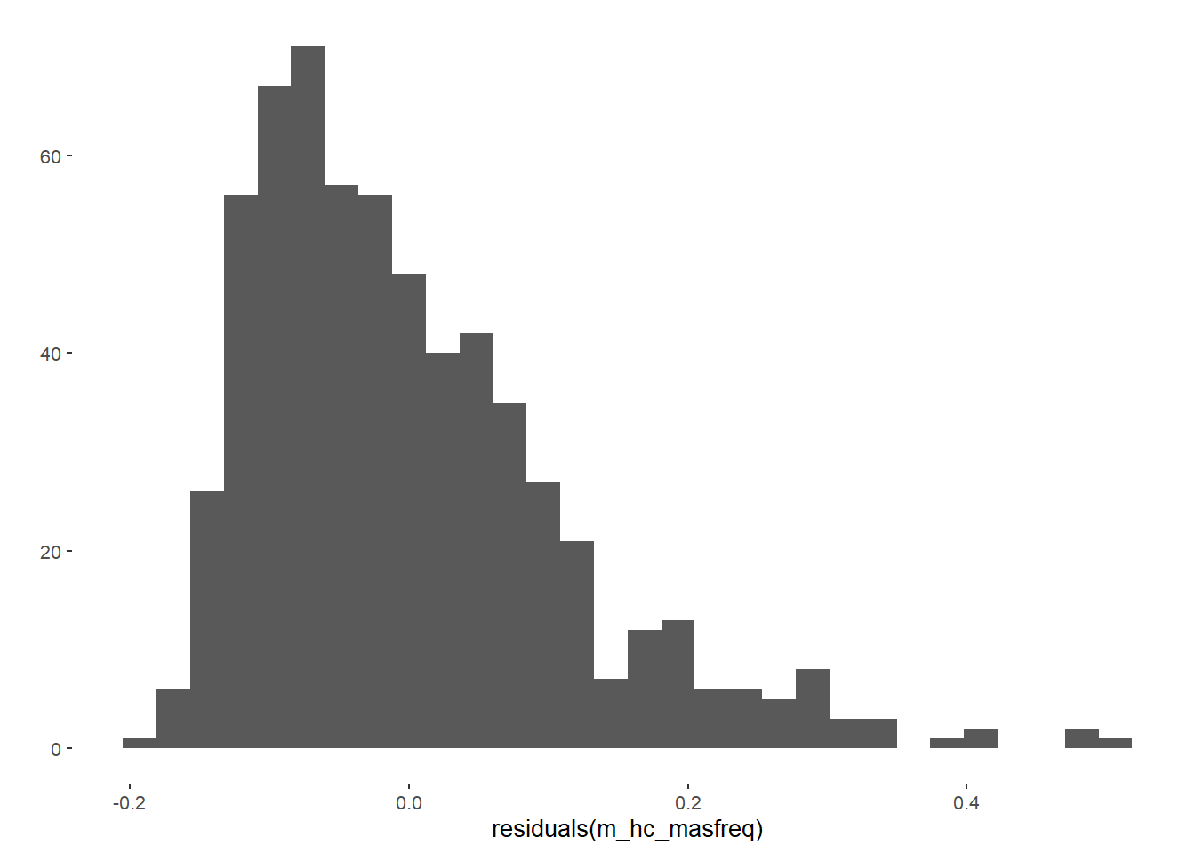
##
## Call:
## lm(formula = diary_masturbation_mean ~ contraception_hormonal_numeric +
## congruent_contraception_numeric + hc_con_interaction + age +
## net_income + relationship_duration_factor + education_years +
## bfi_extra + bfi_neuro + bfi_agree + bfi_consc + bfi_open +
## religiosity, data = data)
##
## Residuals:
## Min 1Q Median 3Q Max
## -0.1950 -0.0847 -0.0263 0.0588 0.5046
##
## Coefficients:
## Estimate Std. Error t value Pr(>|t|)
## (Intercept) 0.131373 0.066043 1.99 0.04713 *
## contraception_hormonal_numeric -0.042567 0.015813 -2.69 0.00730 **
## congruent_contraception_numeric 0.001109 0.013794 0.08 0.93595
## hc_con_interaction 0.014578 0.019803 0.74 0.46193
## age -0.001032 0.001194 -0.86 0.38765
## net_incomeeuro_500_1000 0.017120 0.011913 1.44 0.15122
## net_incomeeuro_1000_2000 0.023694 0.015777 1.50 0.13366
## net_incomeeuro_2000_3000 0.003051 0.022127 0.14 0.89038
## net_incomeeuro_gt_3000 -0.022556 0.037991 -0.59 0.55292
## net_incomedont_tell -0.023805 0.030269 -0.79 0.43192
## relationship_duration_factorPartnered_upto28months 0.001243 0.013251 0.09 0.92531
## relationship_duration_factorPartnered_upto52months -0.003394 0.014294 -0.24 0.81239
## relationship_duration_factorPartnered_morethan52months -0.014246 0.014711 -0.97 0.33323
## education_years 0.000601 0.001074 0.56 0.57616
## bfi_extra -0.002781 0.006505 -0.43 0.66913
## bfi_neuro 0.002272 0.007015 0.32 0.74613
## bfi_agree 0.002357 0.008091 0.29 0.77091
## bfi_consc -0.023510 0.007284 -3.23 0.00132 **
## bfi_open 0.027017 0.007821 3.45 0.00059 ***
## religiosity -0.005825 0.003507 -1.66 0.09727 .
## ---
## Signif. codes: 0 '***' 0.001 '**' 0.01 '*' 0.05 '.' 0.1 ' ' 1
##
## Residual standard error: 0.115 on 602 degrees of freedom
## (557 Beobachtungen als fehlend gelöscht)
## Multiple R-squared: 0.0859, Adjusted R-squared: 0.057
## F-statistic: 2.98 on 19 and 602 DF, p-value: 0.000025## # A tibble: 20 x 7
## term estimate std.error statistic p.value conf.low conf.high
## <chr> <dbl> <dbl> <dbl> <dbl> <dbl> <dbl>
## 1 (Intercept) 1.31e-1 0.0660 1.99 4.71e-2 0.00167 0.261
## 2 contraception_hormonal_numeric -4.26e-2 0.0158 -2.69 7.30e-3 -0.0736 -0.0115
## 3 congruent_contraception_numeric 1.11e-3 0.0138 0.0804 9.36e-1 -0.0260 0.0282
## 4 hc_con_interaction 1.46e-2 0.0198 0.736 4.62e-1 -0.0243 0.0535
## 5 age -1.03e-3 0.00119 -0.865 3.88e-1 -0.00338 0.00131
## 6 net_incomeeuro_500_1000 1.71e-2 0.0119 1.44 1.51e-1 -0.00628 0.0405
## 7 net_incomeeuro_1000_2000 2.37e-2 0.0158 1.50 1.34e-1 -0.00729 0.0547
## 8 net_incomeeuro_2000_3000 3.05e-3 0.0221 0.138 8.90e-1 -0.0404 0.0465
## 9 net_incomeeuro_gt_3000 -2.26e-2 0.0380 -0.594 5.53e-1 -0.0972 0.0521
## 10 net_incomedont_tell -2.38e-2 0.0303 -0.786 4.32e-1 -0.0833 0.0356
## 11 relationship_duration_factorPartnered_upto28months 1.24e-3 0.0133 0.0938 9.25e-1 -0.0248 0.0273
## 12 relationship_duration_factorPartnered_upto52months -3.39e-3 0.0143 -0.237 8.12e-1 -0.0315 0.0247
## 13 relationship_duration_factorPartnered_morethan52months -1.42e-2 0.0147 -0.968 3.33e-1 -0.0431 0.0146
## 14 education_years 6.01e-4 0.00107 0.559 5.76e-1 -0.00151 0.00271
## 15 bfi_extra -2.78e-3 0.00650 -0.428 6.69e-1 -0.0156 0.00999
## 16 bfi_neuro 2.27e-3 0.00701 0.324 7.46e-1 -0.0115 0.0160
## 17 bfi_agree 2.36e-3 0.00809 0.291 7.71e-1 -0.0135 0.0182
## 18 bfi_consc -2.35e-2 0.00728 -3.23 1.32e-3 -0.0378 -0.00920
## 19 bfi_open 2.70e-2 0.00782 3.45 5.90e-4 0.0117 0.0424
## 20 religiosity -5.83e-3 0.00351 -1.66 9.73e-2 -0.0127 0.00106Sensitivity Analyses
HC
m_hc_masfreq_sensitivity_hc <- sensemakr(model = m_hc_masfreq,
treatment = "contraception_hormonal_numeric",
benchmark_covariates = covariates, #covariates that will be
#used to bound the
#plausible strength of the
#unobserved confounders
kd = 1:3, #these arguments parameterize how many times
#stronger the confounder is related to the
#treatment
ky = 1:3, #these arguments parameterize how many times
#stronger the confounder is related to the outcome
q = 1, #fraction of the effect estimate that would have to be
#explained away to be problematic. Setting q = 1,
#means that a reduction of 100% of the current effect
#estimate, that is, a true effect of zero, would be
#deemed problematic.
alpha = 0.05,
reduce = TRUE #confounder reduce absolute effect size
)
m_hc_masfreq_sensitivity_hc## Sensitivity Analysis to Unobserved Confounding
##
## Model Formula: diary_masturbation_mean ~ contraception_hormonal_numeric + congruent_contraception_numeric +
## hc_con_interaction + age + net_income + relationship_duration_factor +
## education_years + bfi_extra + bfi_neuro + bfi_agree + bfi_consc +
## bfi_open + religiosity
##
## Null hypothesis: q = 1 and reduce = TRUE
##
## Unadjusted Estimates of ' contraception_hormonal_numeric ':
## Coef. estimate: -0.043
## Standard Error: 0.016
## t-value: -2.692
##
## Sensitivity Statistics:
## Partial R2 of treatment with outcome: 0.012
## Robustness Value, q = 1 : 0.104
## Robustness Value, q = 1 alpha = 0.05 : 0.029
##
## For more information, check summary.## Sensitivity Analysis to Unobserved Confounding
##
## Model Formula: diary_masturbation_mean ~ contraception_hormonal_numeric + congruent_contraception_numeric +
## hc_con_interaction + age + net_income + relationship_duration_factor +
## education_years + bfi_extra + bfi_neuro + bfi_agree + bfi_consc +
## bfi_open + religiosity
##
## Null hypothesis: q = 1 and reduce = TRUE
## -- This means we are considering biases that reduce the absolute value of the current estimate.
## -- The null hypothesis deemed problematic is H0:tau = 0
##
## Unadjusted Estimates of 'contraception_hormonal_numeric':
## Coef. estimate: -0.043
## Standard Error: 0.016
## t-value (H0:tau = 0): -2.692
##
## Sensitivity Statistics:
## Partial R2 of treatment with outcome: 0.012
## Robustness Value, q = 1: 0.104
## Robustness Value, q = 1, alpha = 0.05: 0.029
##
## Verbal interpretation of sensitivity statistics:
##
## -- Partial R2 of the treatment with the outcome: an extreme confounder (orthogonal to the covariates) that explains 100% of the residual variance of the outcome, would need to explain at least 1.2% of the residual variance of the treatment to fully account for the observed estimated effect.
##
## -- Robustness Value, q = 1: unobserved confounders (orthogonal to the covariates) that explain more than 10.4% of the residual variance of both the treatment and the outcome are strong enough to bring the point estimate to 0 (a bias of 100% of the original estimate). Conversely, unobserved confounders that do not explain more than 10.4% of the residual variance of both the treatment and the outcome are not strong enough to bring the point estimate to 0.
##
## -- Robustness Value, q = 1, alpha = 0.05: unobserved confounders (orthogonal to the covariates) that explain more than 2.9% of the residual variance of both the treatment and the outcome are strong enough to bring the estimate to a range where it is no longer 'statistically different' from 0 (a bias of 100% of the original estimate), at the significance level of alpha = 0.05. Conversely, unobserved confounders that do not explain more than 2.9% of the residual variance of both the treatment and the outcome are not strong enough to bring the estimate to a range where it is no longer 'statistically different' from 0, at the significance level of alpha = 0.05.
##
## Bounds on omitted variable bias:
##
## --The table below shows the maximum strength of unobserved confounders with association with the treatment and the outcome bounded by a multiple of the observed explanatory power of the chosen benchmark covariate(s).
##
## Bound Label R2dz.x R2yz.dx Treatment
## 1x age 0.025 0.001 contraception_hormonal_numeric
## 2x age 0.050 0.003 contraception_hormonal_numeric
## 3x age 0.076 0.004 contraception_hormonal_numeric
## 1x net_incomeeuro_500_1000 0.002 0.003 contraception_hormonal_numeric
## 2x net_incomeeuro_500_1000 0.003 0.007 contraception_hormonal_numeric
## 3x net_incomeeuro_500_1000 0.005 0.010 contraception_hormonal_numeric
## 1x net_incomeeuro_1000_2000 0.001 0.004 contraception_hormonal_numeric
## 2x net_incomeeuro_1000_2000 0.003 0.008 contraception_hormonal_numeric
## 3x net_incomeeuro_1000_2000 0.004 0.011 contraception_hormonal_numeric
## 1x net_incomeeuro_2000_3000 0.000 0.000 contraception_hormonal_numeric
## 2x net_incomeeuro_2000_3000 0.000 0.000 contraception_hormonal_numeric
## 3x net_incomeeuro_2000_3000 0.000 0.000 contraception_hormonal_numeric
## 1x net_incomeeuro_gt_3000 0.001 0.001 contraception_hormonal_numeric
## 2x net_incomeeuro_gt_3000 0.001 0.001 contraception_hormonal_numeric
## 3x net_incomeeuro_gt_3000 0.002 0.002 contraception_hormonal_numeric
## 1x net_incomedont_tell 0.001 0.001 contraception_hormonal_numeric
## 2x net_incomedont_tell 0.003 0.002 contraception_hormonal_numeric
## 3x net_incomedont_tell 0.004 0.003 contraception_hormonal_numeric
## 1x relationship_duration_factorPartnered_upto28months 0.001 0.000 contraception_hormonal_numeric
## 2x relationship_duration_factorPartnered_upto28months 0.002 0.000 contraception_hormonal_numeric
## 3x relationship_duration_factorPartnered_upto28months 0.003 0.000 contraception_hormonal_numeric
## 1x relationship_duration_factorPartnered_upto52months 0.002 0.000 contraception_hormonal_numeric
## 2x relationship_duration_factorPartnered_upto52months 0.003 0.000 contraception_hormonal_numeric
## 3x relationship_duration_factorPartnered_upto52months 0.005 0.000 contraception_hormonal_numeric
## 1x relationship_duration_factorPartnered_morethan52months 0.001 0.002 contraception_hormonal_numeric
## 2x relationship_duration_factorPartnered_morethan52months 0.003 0.003 contraception_hormonal_numeric
## 3x relationship_duration_factorPartnered_morethan52months 0.004 0.005 contraception_hormonal_numeric
## 1x education_years 0.011 0.001 contraception_hormonal_numeric
## 2x education_years 0.021 0.001 contraception_hormonal_numeric
## 3x education_years 0.032 0.002 contraception_hormonal_numeric
## 1x bfi_extra 0.000 0.000 contraception_hormonal_numeric
## 2x bfi_extra 0.000 0.001 contraception_hormonal_numeric
## 3x bfi_extra 0.000 0.001 contraception_hormonal_numeric
## 1x bfi_neuro 0.002 0.000 contraception_hormonal_numeric
## 2x bfi_neuro 0.004 0.000 contraception_hormonal_numeric
## 3x bfi_neuro 0.006 0.001 contraception_hormonal_numeric
## 1x bfi_agree 0.010 0.000 contraception_hormonal_numeric
## 2x bfi_agree 0.020 0.000 contraception_hormonal_numeric
## 3x bfi_agree 0.030 0.000 contraception_hormonal_numeric
## 1x bfi_consc 0.002 0.017 contraception_hormonal_numeric
## 2x bfi_consc 0.003 0.035 contraception_hormonal_numeric
## 3x bfi_consc 0.005 0.052 contraception_hormonal_numeric
## 1x bfi_open 0.001 0.020 contraception_hormonal_numeric
## 2x bfi_open 0.001 0.040 contraception_hormonal_numeric
## 3x bfi_open 0.002 0.060 contraception_hormonal_numeric
## 1x religiosity 0.002 0.005 contraception_hormonal_numeric
## 2x religiosity 0.005 0.009 contraception_hormonal_numeric
## 3x religiosity 0.007 0.014 contraception_hormonal_numeric
## Adjusted Estimate Adjusted Se Adjusted T Adjusted Lower CI Adjusted Upper CI
## -0.040 0.016 -2.516 -0.072 -0.009
## -0.038 0.016 -2.342 -0.070 -0.006
## -0.036 0.016 -2.167 -0.068 -0.003
## -0.042 0.016 -2.636 -0.073 -0.011
## -0.041 0.016 -2.583 -0.072 -0.010
## -0.040 0.016 -2.529 -0.071 -0.009
## -0.042 0.016 -2.635 -0.073 -0.011
## -0.041 0.016 -2.580 -0.072 -0.010
## -0.040 0.016 -2.524 -0.071 -0.009
## -0.043 0.016 -2.689 -0.074 -0.011
## -0.043 0.016 -2.689 -0.074 -0.011
## -0.043 0.016 -2.689 -0.074 -0.011
## -0.042 0.016 -2.674 -0.073 -0.011
## -0.042 0.016 -2.658 -0.073 -0.011
## -0.042 0.016 -2.642 -0.073 -0.011
## -0.042 0.016 -2.661 -0.073 -0.011
## -0.042 0.016 -2.631 -0.073 -0.011
## -0.041 0.016 -2.602 -0.072 -0.010
## -0.043 0.016 -2.685 -0.074 -0.011
## -0.042 0.016 -2.681 -0.074 -0.011
## -0.042 0.016 -2.677 -0.074 -0.011
## -0.042 0.016 -2.678 -0.074 -0.011
## -0.042 0.016 -2.667 -0.073 -0.011
## -0.042 0.016 -2.655 -0.073 -0.011
## -0.042 0.016 -2.652 -0.073 -0.011
## -0.041 0.016 -2.615 -0.072 -0.010
## -0.041 0.016 -2.578 -0.072 -0.010
## -0.042 0.016 -2.618 -0.073 -0.010
## -0.041 0.016 -2.546 -0.072 -0.009
## -0.040 0.016 -2.475 -0.071 -0.008
## -0.043 0.016 -2.688 -0.074 -0.011
## -0.043 0.016 -2.687 -0.074 -0.011
## -0.042 0.016 -2.685 -0.074 -0.011
## -0.042 0.016 -2.673 -0.073 -0.011
## -0.042 0.016 -2.655 -0.073 -0.011
## -0.042 0.016 -2.638 -0.073 -0.011
## -0.042 0.016 -2.647 -0.073 -0.011
## -0.042 0.016 -2.604 -0.073 -0.010
## -0.041 0.016 -2.561 -0.073 -0.010
## -0.040 0.016 -2.575 -0.071 -0.010
## -0.038 0.016 -2.458 -0.069 -0.008
## -0.036 0.015 -2.340 -0.066 -0.006
## -0.041 0.016 -2.625 -0.072 -0.010
## -0.040 0.016 -2.559 -0.070 -0.009
## -0.038 0.015 -2.492 -0.068 -0.008
## -0.041 0.016 -2.609 -0.072 -0.010
## -0.040 0.016 -2.528 -0.071 -0.009
## -0.039 0.016 -2.447 -0.070 -0.008Congreuncy
m_hc_masfreq_sensitivity_con <- sensemakr(model = m_hc_masfreq,
treatment = "congruent_contraception_numeric",
benchmark_covariates = covariates, #covariates that will be
#used to bound the
#plausible strength of the
#unobserved confounders
kd = 1:3, #these arguments parameterize how many times
#stronger the confounder is related to the
#treatment
ky = 1:3, #these arguments parameterize how many times
#stronger the confounder is related to the outcome
q = 1, #fraction of the effect estimate that would have to be
#explained away to be problematic. Setting q = 1,
#means that a reduction of 100% of the current effect
#estimate, that is, a true effect of zero, would be
#deemed problematic.
alpha = 0.05,
reduce = TRUE #confounder reduce absolute effect size
)
m_hc_masfreq_sensitivity_con## Sensitivity Analysis to Unobserved Confounding
##
## Model Formula: diary_masturbation_mean ~ contraception_hormonal_numeric + congruent_contraception_numeric +
## hc_con_interaction + age + net_income + relationship_duration_factor +
## education_years + bfi_extra + bfi_neuro + bfi_agree + bfi_consc +
## bfi_open + religiosity
##
## Null hypothesis: q = 1 and reduce = TRUE
##
## Unadjusted Estimates of ' congruent_contraception_numeric ':
## Coef. estimate: 0.001
## Standard Error: 0.014
## t-value: 0.08
##
## Sensitivity Statistics:
## Partial R2 of treatment with outcome: 0
## Robustness Value, q = 1 : 0.003
## Robustness Value, q = 1 alpha = 0.05 : 0
##
## For more information, check summary.## Sensitivity Analysis to Unobserved Confounding
##
## Model Formula: diary_masturbation_mean ~ contraception_hormonal_numeric + congruent_contraception_numeric +
## hc_con_interaction + age + net_income + relationship_duration_factor +
## education_years + bfi_extra + bfi_neuro + bfi_agree + bfi_consc +
## bfi_open + religiosity
##
## Null hypothesis: q = 1 and reduce = TRUE
## -- This means we are considering biases that reduce the absolute value of the current estimate.
## -- The null hypothesis deemed problematic is H0:tau = 0
##
## Unadjusted Estimates of 'congruent_contraception_numeric':
## Coef. estimate: 0.001
## Standard Error: 0.014
## t-value (H0:tau = 0): 0.08
##
## Sensitivity Statistics:
## Partial R2 of treatment with outcome: 0
## Robustness Value, q = 1: 0.003
## Robustness Value, q = 1, alpha = 0.05: 0
##
## Verbal interpretation of sensitivity statistics:
##
## -- Partial R2 of the treatment with the outcome: an extreme confounder (orthogonal to the covariates) that explains 100% of the residual variance of the outcome, would need to explain at least 0% of the residual variance of the treatment to fully account for the observed estimated effect.
##
## -- Robustness Value, q = 1: unobserved confounders (orthogonal to the covariates) that explain more than 0.3% of the residual variance of both the treatment and the outcome are strong enough to bring the point estimate to 0 (a bias of 100% of the original estimate). Conversely, unobserved confounders that do not explain more than 0.3% of the residual variance of both the treatment and the outcome are not strong enough to bring the point estimate to 0.
##
## -- Robustness Value, q = 1, alpha = 0.05: unobserved confounders (orthogonal to the covariates) that explain more than 0% of the residual variance of both the treatment and the outcome are strong enough to bring the estimate to a range where it is no longer 'statistically different' from 0 (a bias of 100% of the original estimate), at the significance level of alpha = 0.05. Conversely, unobserved confounders that do not explain more than 0% of the residual variance of both the treatment and the outcome are not strong enough to bring the estimate to a range where it is no longer 'statistically different' from 0, at the significance level of alpha = 0.05.
##
## Bounds on omitted variable bias:
##
## --The table below shows the maximum strength of unobserved confounders with association with the treatment and the outcome bounded by a multiple of the observed explanatory power of the chosen benchmark covariate(s).
##
## Bound Label R2dz.x R2yz.dx Treatment
## 1x age 0.003 0.001 congruent_contraception_numeric
## 2x age 0.006 0.002 congruent_contraception_numeric
## 3x age 0.009 0.004 congruent_contraception_numeric
## 1x net_incomeeuro_500_1000 0.001 0.003 congruent_contraception_numeric
## 2x net_incomeeuro_500_1000 0.001 0.007 congruent_contraception_numeric
## 3x net_incomeeuro_500_1000 0.002 0.010 congruent_contraception_numeric
## 1x net_incomeeuro_1000_2000 0.002 0.004 congruent_contraception_numeric
## 2x net_incomeeuro_1000_2000 0.004 0.008 congruent_contraception_numeric
## 3x net_incomeeuro_1000_2000 0.005 0.011 congruent_contraception_numeric
## 1x net_incomeeuro_2000_3000 0.005 0.000 congruent_contraception_numeric
## 2x net_incomeeuro_2000_3000 0.011 0.000 congruent_contraception_numeric
## 3x net_incomeeuro_2000_3000 0.016 0.000 congruent_contraception_numeric
## 1x net_incomeeuro_gt_3000 0.001 0.001 congruent_contraception_numeric
## 2x net_incomeeuro_gt_3000 0.002 0.001 congruent_contraception_numeric
## 3x net_incomeeuro_gt_3000 0.003 0.002 congruent_contraception_numeric
## 1x net_incomedont_tell 0.000 0.001 congruent_contraception_numeric
## 2x net_incomedont_tell 0.000 0.002 congruent_contraception_numeric
## 3x net_incomedont_tell 0.000 0.003 congruent_contraception_numeric
## 1x relationship_duration_factorPartnered_upto28months 0.016 0.000 congruent_contraception_numeric
## 2x relationship_duration_factorPartnered_upto28months 0.032 0.000 congruent_contraception_numeric
## 3x relationship_duration_factorPartnered_upto28months 0.048 0.000 congruent_contraception_numeric
## 1x relationship_duration_factorPartnered_upto52months 0.065 0.000 congruent_contraception_numeric
## 2x relationship_duration_factorPartnered_upto52months 0.131 0.000 congruent_contraception_numeric
## 3x relationship_duration_factorPartnered_upto52months 0.196 0.000 congruent_contraception_numeric
## 1x relationship_duration_factorPartnered_morethan52months 0.080 0.002 congruent_contraception_numeric
## 2x relationship_duration_factorPartnered_morethan52months 0.161 0.004 congruent_contraception_numeric
## 3x relationship_duration_factorPartnered_morethan52months 0.241 0.006 congruent_contraception_numeric
## 1x education_years 0.012 0.001 congruent_contraception_numeric
## 2x education_years 0.023 0.001 congruent_contraception_numeric
## 3x education_years 0.035 0.002 congruent_contraception_numeric
## 1x bfi_extra 0.000 0.000 congruent_contraception_numeric
## 2x bfi_extra 0.000 0.001 congruent_contraception_numeric
## 3x bfi_extra 0.000 0.001 congruent_contraception_numeric
## 1x bfi_neuro 0.003 0.000 congruent_contraception_numeric
## 2x bfi_neuro 0.005 0.000 congruent_contraception_numeric
## 3x bfi_neuro 0.008 0.001 congruent_contraception_numeric
## 1x bfi_agree 0.002 0.000 congruent_contraception_numeric
## 2x bfi_agree 0.003 0.000 congruent_contraception_numeric
## 3x bfi_agree 0.005 0.000 congruent_contraception_numeric
## 1x bfi_consc 0.000 0.017 congruent_contraception_numeric
## 2x bfi_consc 0.000 0.035 congruent_contraception_numeric
## 3x bfi_consc 0.001 0.052 congruent_contraception_numeric
## 1x bfi_open 0.001 0.020 congruent_contraception_numeric
## 2x bfi_open 0.001 0.040 congruent_contraception_numeric
## 3x bfi_open 0.002 0.060 congruent_contraception_numeric
## 1x religiosity 0.001 0.005 congruent_contraception_numeric
## 2x religiosity 0.002 0.009 congruent_contraception_numeric
## 3x religiosity 0.003 0.014 congruent_contraception_numeric
## Adjusted Estimate Adjusted Se Adjusted T Adjusted Lower CI Adjusted Upper CI
## 0.000 0.014 0.032 -0.027 0.028
## 0.000 0.014 -0.016 -0.027 0.027
## -0.001 0.014 -0.064 -0.028 0.026
## 0.001 0.014 0.045 -0.026 0.028
## 0.000 0.014 0.010 -0.027 0.027
## 0.000 0.014 -0.026 -0.027 0.027
## 0.000 0.014 0.016 -0.027 0.027
## -0.001 0.014 -0.049 -0.028 0.026
## -0.002 0.014 -0.113 -0.029 0.025
## 0.001 0.014 0.070 -0.026 0.028
## 0.001 0.014 0.060 -0.026 0.028
## 0.001 0.014 0.049 -0.027 0.028
## 0.001 0.014 0.062 -0.026 0.028
## 0.001 0.014 0.043 -0.027 0.028
## 0.000 0.014 0.024 -0.027 0.027
## 0.001 0.014 0.077 -0.026 0.028
## 0.001 0.014 0.073 -0.026 0.028
## 0.001 0.014 0.069 -0.026 0.028
## 0.001 0.014 0.068 -0.026 0.028
## 0.001 0.014 0.055 -0.027 0.028
## 0.001 0.014 0.042 -0.027 0.028
## 0.000 0.014 0.013 -0.028 0.028
## -0.001 0.015 -0.055 -0.030 0.028
## -0.002 0.015 -0.124 -0.032 0.028
## -0.003 0.014 -0.221 -0.031 0.025
## -0.008 0.015 -0.526 -0.037 0.022
## -0.013 0.016 -0.838 -0.044 0.018
## 0.000 0.014 0.019 -0.027 0.028
## -0.001 0.014 -0.043 -0.028 0.027
## -0.001 0.014 -0.105 -0.029 0.026
## 0.001 0.014 0.079 -0.026 0.028
## 0.001 0.014 0.078 -0.026 0.028
## 0.001 0.014 0.077 -0.026 0.028
## 0.001 0.014 0.063 -0.026 0.028
## 0.001 0.014 0.046 -0.027 0.028
## 0.000 0.014 0.029 -0.027 0.028
## 0.001 0.014 0.068 -0.026 0.028
## 0.001 0.014 0.057 -0.026 0.028
## 0.001 0.014 0.045 -0.027 0.028
## 0.000 0.014 0.031 -0.026 0.027
## 0.000 0.014 -0.018 -0.027 0.026
## -0.001 0.013 -0.069 -0.027 0.025
## 0.000 0.014 0.002 -0.027 0.027
## -0.001 0.014 -0.079 -0.028 0.026
## -0.002 0.013 -0.161 -0.028 0.024
## 0.000 0.014 0.028 -0.027 0.027
## 0.000 0.014 -0.025 -0.027 0.027
## -0.001 0.014 -0.078 -0.028 0.026Interaction
m_hc_masfreq_sensitivity_interaction <- sensemakr(model = m_hc_masfreq,
treatment = "hc_con_interaction",
benchmark_covariates = covariates, #covariates that will be
#used to bound the
#plausible strength of the
#unobserved confounders
kd = 1:3, #these arguments parameterize how many times
#stronger the confounder is related to the
#treatment
ky = 1:3, #these arguments parameterize how many times
#stronger the confounder is related to the outcome
q = 1, #fraction of the effect estimate that would have to be
#explained away to be problematic. Setting q = 1,
#means that a reduction of 100% of the current effect
#estimate, that is, a true effect of zero, would be
#deemed problematic.
alpha = 0.05,
reduce = TRUE #confounder reduce absolute effect size
)
m_hc_masfreq_sensitivity_interaction## Sensitivity Analysis to Unobserved Confounding
##
## Model Formula: diary_masturbation_mean ~ contraception_hormonal_numeric + congruent_contraception_numeric +
## hc_con_interaction + age + net_income + relationship_duration_factor +
## education_years + bfi_extra + bfi_neuro + bfi_agree + bfi_consc +
## bfi_open + religiosity
##
## Null hypothesis: q = 1 and reduce = TRUE
##
## Unadjusted Estimates of ' hc_con_interaction ':
## Coef. estimate: 0.015
## Standard Error: 0.02
## t-value: 0.736
##
## Sensitivity Statistics:
## Partial R2 of treatment with outcome: 0.001
## Robustness Value, q = 1 : 0.03
## Robustness Value, q = 1 alpha = 0.05 : 0
##
## For more information, check summary.## Sensitivity Analysis to Unobserved Confounding
##
## Model Formula: diary_masturbation_mean ~ contraception_hormonal_numeric + congruent_contraception_numeric +
## hc_con_interaction + age + net_income + relationship_duration_factor +
## education_years + bfi_extra + bfi_neuro + bfi_agree + bfi_consc +
## bfi_open + religiosity
##
## Null hypothesis: q = 1 and reduce = TRUE
## -- This means we are considering biases that reduce the absolute value of the current estimate.
## -- The null hypothesis deemed problematic is H0:tau = 0
##
## Unadjusted Estimates of 'hc_con_interaction':
## Coef. estimate: 0.015
## Standard Error: 0.02
## t-value (H0:tau = 0): 0.736
##
## Sensitivity Statistics:
## Partial R2 of treatment with outcome: 0.001
## Robustness Value, q = 1: 0.03
## Robustness Value, q = 1, alpha = 0.05: 0
##
## Verbal interpretation of sensitivity statistics:
##
## -- Partial R2 of the treatment with the outcome: an extreme confounder (orthogonal to the covariates) that explains 100% of the residual variance of the outcome, would need to explain at least 0.1% of the residual variance of the treatment to fully account for the observed estimated effect.
##
## -- Robustness Value, q = 1: unobserved confounders (orthogonal to the covariates) that explain more than 3% of the residual variance of both the treatment and the outcome are strong enough to bring the point estimate to 0 (a bias of 100% of the original estimate). Conversely, unobserved confounders that do not explain more than 3% of the residual variance of both the treatment and the outcome are not strong enough to bring the point estimate to 0.
##
## -- Robustness Value, q = 1, alpha = 0.05: unobserved confounders (orthogonal to the covariates) that explain more than 0% of the residual variance of both the treatment and the outcome are strong enough to bring the estimate to a range where it is no longer 'statistically different' from 0 (a bias of 100% of the original estimate), at the significance level of alpha = 0.05. Conversely, unobserved confounders that do not explain more than 0% of the residual variance of both the treatment and the outcome are not strong enough to bring the estimate to a range where it is no longer 'statistically different' from 0, at the significance level of alpha = 0.05.
##
## Bounds on omitted variable bias:
##
## --The table below shows the maximum strength of unobserved confounders with association with the treatment and the outcome bounded by a multiple of the observed explanatory power of the chosen benchmark covariate(s).
##
## Bound Label R2dz.x R2yz.dx Treatment
## 1x age 0.000 0.001 hc_con_interaction
## 2x age 0.001 0.002 hc_con_interaction
## 3x age 0.001 0.004 hc_con_interaction
## 1x net_incomeeuro_500_1000 0.000 0.003 hc_con_interaction
## 2x net_incomeeuro_500_1000 0.000 0.007 hc_con_interaction
## 3x net_incomeeuro_500_1000 0.001 0.010 hc_con_interaction
## 1x net_incomeeuro_1000_2000 0.002 0.004 hc_con_interaction
## 2x net_incomeeuro_1000_2000 0.004 0.008 hc_con_interaction
## 3x net_incomeeuro_1000_2000 0.006 0.011 hc_con_interaction
## 1x net_incomeeuro_2000_3000 0.000 0.000 hc_con_interaction
## 2x net_incomeeuro_2000_3000 0.001 0.000 hc_con_interaction
## 3x net_incomeeuro_2000_3000 0.001 0.000 hc_con_interaction
## 1x net_incomeeuro_gt_3000 0.000 0.001 hc_con_interaction
## 2x net_incomeeuro_gt_3000 0.000 0.001 hc_con_interaction
## 3x net_incomeeuro_gt_3000 0.000 0.002 hc_con_interaction
## 1x net_incomedont_tell 0.002 0.001 hc_con_interaction
## 2x net_incomedont_tell 0.004 0.002 hc_con_interaction
## 3x net_incomedont_tell 0.005 0.003 hc_con_interaction
## 1x relationship_duration_factorPartnered_upto28months 0.006 0.000 hc_con_interaction
## 2x relationship_duration_factorPartnered_upto28months 0.012 0.000 hc_con_interaction
## 3x relationship_duration_factorPartnered_upto28months 0.017 0.000 hc_con_interaction
## 1x relationship_duration_factorPartnered_upto52months 0.009 0.000 hc_con_interaction
## 2x relationship_duration_factorPartnered_upto52months 0.018 0.000 hc_con_interaction
## 3x relationship_duration_factorPartnered_upto52months 0.027 0.000 hc_con_interaction
## 1x relationship_duration_factorPartnered_morethan52months 0.019 0.002 hc_con_interaction
## 2x relationship_duration_factorPartnered_morethan52months 0.037 0.003 hc_con_interaction
## 3x relationship_duration_factorPartnered_morethan52months 0.056 0.005 hc_con_interaction
## 1x education_years 0.015 0.001 hc_con_interaction
## 2x education_years 0.029 0.001 hc_con_interaction
## 3x education_years 0.044 0.002 hc_con_interaction
## 1x bfi_extra 0.000 0.000 hc_con_interaction
## 2x bfi_extra 0.000 0.001 hc_con_interaction
## 3x bfi_extra 0.001 0.001 hc_con_interaction
## 1x bfi_neuro 0.001 0.000 hc_con_interaction
## 2x bfi_neuro 0.002 0.000 hc_con_interaction
## 3x bfi_neuro 0.004 0.001 hc_con_interaction
## 1x bfi_agree 0.006 0.000 hc_con_interaction
## 2x bfi_agree 0.012 0.000 hc_con_interaction
## 3x bfi_agree 0.019 0.000 hc_con_interaction
## 1x bfi_consc 0.001 0.017 hc_con_interaction
## 2x bfi_consc 0.003 0.035 hc_con_interaction
## 3x bfi_consc 0.004 0.052 hc_con_interaction
## 1x bfi_open 0.004 0.020 hc_con_interaction
## 2x bfi_open 0.008 0.040 hc_con_interaction
## 3x bfi_open 0.012 0.060 hc_con_interaction
## 1x religiosity 0.006 0.005 hc_con_interaction
## 2x religiosity 0.012 0.009 hc_con_interaction
## 3x religiosity 0.018 0.014 hc_con_interaction
## Adjusted Estimate Adjusted Se Adjusted T Adjusted Lower CI Adjusted Upper CI
## 0.014 0.020 0.720 -0.025 0.053
## 0.014 0.020 0.705 -0.025 0.053
## 0.014 0.020 0.690 -0.025 0.053
## 0.014 0.020 0.718 -0.025 0.053
## 0.014 0.020 0.700 -0.025 0.053
## 0.013 0.020 0.682 -0.025 0.052
## 0.013 0.020 0.667 -0.026 0.052
## 0.012 0.020 0.599 -0.027 0.051
## 0.010 0.020 0.530 -0.028 0.049
## 0.015 0.020 0.733 -0.024 0.053
## 0.014 0.020 0.730 -0.024 0.053
## 0.014 0.020 0.727 -0.025 0.053
## 0.014 0.020 0.732 -0.024 0.053
## 0.014 0.020 0.728 -0.024 0.053
## 0.014 0.020 0.724 -0.025 0.053
## 0.014 0.020 0.702 -0.025 0.053
## 0.013 0.020 0.668 -0.026 0.052
## 0.013 0.020 0.634 -0.026 0.052
## 0.014 0.020 0.726 -0.025 0.053
## 0.014 0.020 0.717 -0.025 0.053
## 0.014 0.020 0.708 -0.025 0.053
## 0.014 0.020 0.710 -0.025 0.053
## 0.014 0.020 0.684 -0.026 0.053
## 0.013 0.020 0.658 -0.026 0.053
## 0.012 0.020 0.594 -0.027 0.051
## 0.009 0.020 0.453 -0.030 0.049
## 0.006 0.020 0.311 -0.034 0.046
## 0.013 0.020 0.662 -0.026 0.052
## 0.012 0.020 0.588 -0.028 0.051
## 0.010 0.020 0.514 -0.029 0.050
## 0.014 0.020 0.729 -0.024 0.053
## 0.014 0.020 0.723 -0.025 0.053
## 0.014 0.020 0.717 -0.025 0.053
## 0.014 0.020 0.724 -0.025 0.053
## 0.014 0.020 0.712 -0.025 0.053
## 0.014 0.020 0.701 -0.025 0.053
## 0.014 0.020 0.710 -0.025 0.053
## 0.014 0.020 0.685 -0.026 0.053
## 0.013 0.020 0.659 -0.026 0.052
## 0.012 0.020 0.620 -0.026 0.051
## 0.010 0.020 0.502 -0.029 0.048
## 0.007 0.019 0.383 -0.031 0.045
## 0.010 0.020 0.519 -0.028 0.049
## 0.006 0.019 0.298 -0.032 0.044
## 0.001 0.019 0.072 -0.037 0.039
## 0.012 0.020 0.607 -0.027 0.051
## 0.009 0.020 0.477 -0.030 0.048
## 0.007 0.020 0.347 -0.032 0.046LS0tDQp0aXRsZTogIlNlbnNpdGl2aXR5IEFuYWx5c2lzIg0Kb3V0cHV0Og0KICBodG1sX2RvY3VtZW50Og0KICAgIHRvYzogdHJ1ZQ0KICAgIHRvY19kZXB0aDogNA0KICAgIHRvY19mbG9hdDogdHJ1ZQ0KICAgIGNvZGVfZm9sZGluZzogJ2hpZGUnDQogICAgc2VsZl9jb250YWluZWQ6IGZhbHNlDQotLS0NCiAgDQogIA0KIyMgRGF0YSANCmBgYHtyIHJlc3VsdHM9J2hpZGUnLG1lc3NhZ2U9Rix3YXJuaW5nPUZ9DQpzb3VyY2UoIjBfaGVscGVycy5SIikNCg0KbG9hZCgiZGF0YS9jbGVhbmVkX3NlbGVjdGVkX3dyYW5nbGVkLnJkYXRhIikNCmBgYA0KDQojIyBQcmVwYXJhdGlvbnMgey50YWJzZXR9DQojIyMgQ2hhbmdlIGZhY3RvcnMgdG8gbnVtZXJpY3MsIGhhbmRjb2RlIGludGVyYWN0aW9uDQpgYGB7cn0NCmRhdGEgPSBkYXRhICU+JQ0KICBtdXRhdGUoY29udHJhY2VwdGlvbl9ob3Jtb25hbF9udW1lcmljID0gaWZlbHNlKGNvbnRyYWNlcHRpb25faG9ybW9uYWwgPT0gInllcyIsDQogICAgICAgICAgICAgICAgICAgICAgICAgICAgICAgICAgICAgICAgICAgICAgICAgMSwNCiAgICAgICAgICAgICAgICAgICAgICAgICAgICAgICAgICAgICAgICAgICAgICAgICBpZmVsc2UoY29udHJhY2VwdGlvbl9ob3Jtb25hbCA9PSAibm8iLA0KICAgICAgICAgICAgICAgICAgICAgICAgICAgICAgICAgICAgICAgICAgICAgICAgICAgICAgICAwLCBOQSkpLA0KICAgICAgICAgY29uZ3J1ZW50X2NvbnRyYWNlcHRpb25fbnVtZXJpYyA9IGlmZWxzZShjb25ncnVlbnRfY29udHJhY2VwdGlvbiA9PSAiMCIsDQogICAgICAgICAgICAgICAgICAgICAgICAgICAgICAgICAgICAgICAgICAgICAgICAgIDAsDQogICAgICAgICAgICAgICAgICAgICAgICAgICAgICAgICAgICAgICAgICAgICAgICAgIGlmZWxzZShjb25ncnVlbnRfY29udHJhY2VwdGlvbiA9PSAiMSIsDQogICAgICAgICAgICAgICAgICAgICAgICAgICAgICAgICAgICAgICAgICAgICAgICAgICAgICAgICAxLCBOQSkpLA0KICAgICAgICAgaGNfY29uX2ludGVyYWN0aW9uID0gaWZlbHNlKGlzLm5hKGNvbmdydWVudF9jb250cmFjZXB0aW9uKSwgTkEsDQogICAgICAgICAgICAgICAgICAgICAgICAgICAgICAgICAgICAgaWZlbHNlKGNvbnRyYWNlcHRpb25faG9ybW9uYWwgPT0gInllcyIgJg0KICAgICAgICAgICAgICAgICAgICAgICAgICAgICAgICAgICAgICAgICAgICAgIGNvbmdydWVudF9jb250cmFjZXB0aW9uID09ICIxIiwgMSwgMCkpKQ0KYGBgDQoNCiMjIyBDb3ZhcmlhdGVzDQpgYGB7cn0NCmNvdmFyaWF0ZXMgPSBsaXN0KCJhZ2UiLA0KICAgICAgICAgICAgICAgICAgICJuZXRfaW5jb21lZXVyb181MDBfMTAwMCIsICJuZXRfaW5jb21lZXVyb18xMDAwXzIwMDAiLA0KICAgICAgICAgICAgICAgICAgICJuZXRfaW5jb21lZXVyb18yMDAwXzMwMDAiLCAibmV0X2luY29tZWV1cm9fZ3RfMzAwMCIsDQogICAgICAgICAgICAgICAgICAgICJuZXRfaW5jb21lZG9udF90ZWxsIiwNCiAgICAgICAgICAgICAgICAgICAicmVsYXRpb25zaGlwX2R1cmF0aW9uX2ZhY3RvclBhcnRuZXJlZF91cHRvMjhtb250aHMiLA0KICAgICAgICAgICAgICAgICAgICJyZWxhdGlvbnNoaXBfZHVyYXRpb25fZmFjdG9yUGFydG5lcmVkX3VwdG81Mm1vbnRocyIsDQogICAgICAgICAgICAgICAgICAgInJlbGF0aW9uc2hpcF9kdXJhdGlvbl9mYWN0b3JQYXJ0bmVyZWRfbW9yZXRoYW41Mm1vbnRocyIsDQogICAgICAgICAgICAgICAgICAgImVkdWNhdGlvbl95ZWFycyIsICJiZmlfZXh0cmEiLCAiYmZpX25ldXJvIiwgImJmaV9hZ3JlZSIsDQogICAgICAgICAgICAgICAgICAgImJmaV9jb25zYyIsICJiZmlfb3BlbiIsICJyZWxpZ2lvc2l0eSIpDQpuYW1lcyhjb3ZhcmlhdGVzKSA9IGMoImFnZSIsDQogICAgICAgICAgICAgICAgICAgIm5ldF9pbmNvbWVldXJvXzUwMF8xMDAwIiwgIm5ldF9pbmNvbWVldXJvXzEwMDBfMjAwMCIsDQogICAgICAgICAgICAgICAgICAgIm5ldF9pbmNvbWVldXJvXzIwMDBfMzAwMCIsICJuZXRfaW5jb21lZXVyb19ndF8zMDAwIiwNCiAgICAgICAgICAgICAgICAgICAgIm5ldF9pbmNvbWVkb250X3RlbGwiLA0KICAgICAgICAgICAgICAgICAgICJyZWxhdGlvbnNoaXBfZHVyYXRpb25fZmFjdG9yUGFydG5lcmVkX3VwdG8yOG1vbnRocyIsDQogICAgICAgICAgICAgICAgICAgInJlbGF0aW9uc2hpcF9kdXJhdGlvbl9mYWN0b3JQYXJ0bmVyZWRfdXB0bzUybW9udGhzIiwNCiAgICAgICAgICAgICAgICAgICAicmVsYXRpb25zaGlwX2R1cmF0aW9uX2ZhY3RvclBhcnRuZXJlZF9tb3JldGhhbjUybW9udGhzIiwNCiAgICAgICAgICAgICAgICAgICAiZWR1Y2F0aW9uX3llYXJzIiwgImJmaV9leHRyYSIsICJiZmlfbmV1cm8iLCAiYmZpX2FncmVlIiwNCiAgICAgICAgICAgICAgICAgICAiYmZpX2NvbnNjIiwgImJmaV9vcGVuIiwgInJlbGlnaW9zaXR5IikNCmBgYA0KDQojIyBFZmZlY3RzIG9mIEhvcm1vbmFsIENvbnRyYWNlcHRpb24gIHsudGFic2V0fQ0KIyMjIEF0dHJhY3RpdmVuZXNzIG9mIFBhcnRuZXIgey50YWJzZXR9DQojIyMjIFVuY29udHJvbGxlZCBNb2RlbCB7LnRhYnNldH0NCiMjIyMjIE1vZGVsDQpgYGB7cn0NCm1faGNfYXRyciA9IGxtKGF0dHJhY3RpdmVuZXNzX3BhcnRuZXIgfiBjb250cmFjZXB0aW9uX2hvcm1vbmFsX251bWVyaWMsDQogICAgICAgICAgICAgICBkYXRhID0gZGF0YSkNCnN1bW1hcnkobV9oY19hdHJyKQ0KdGlkeShtX2hjX2F0cnIpDQpgYGANCg0KIyMjIyMgU2Vuc2l0aXZpdHkgQW5hbHlzZXMNCmBgYHtyfQ0KbV9oY19hdHJyX3NlbnNpdGl2aXR5IDwtIHNlbnNlbWFrcihtb2RlbCA9IG1faGNfYXRyciwgI21vZGVsDQogICAgICAgICAgICAgICAgICAgICAgICAgICAgICAgIHRyZWF0bWVudCA9ICJjb250cmFjZXB0aW9uX2hvcm1vbmFsX251bWVyaWMiLCAjcHJlZGljdG9yDQogICAgICAgICAgICAgICAgICAgICAgICAgICAgICAgIGtkID0gMTozLCAjdGhlc2UgYXJndW1lbnRzIHBhcmFtZXRlcml6ZSBob3cgbWFueSB0aW1lcw0KICAgICAgICAgICAgICAgICAgICAgICAgICAgICAgICAgICAgICAgICAgI3N0cm9uZ2VyIHRoZSBjb25mb3VuZGVyIGlzIHJlbGF0ZWQgdG8gdGhlDQogICAgICAgICAgICAgICAgICAgICAgICAgICAgICAgICAgICAgICAgICAjdHJlYXRtZW50DQogICAgICAgICAgICAgICAgICAgICAgICAgICAgICAgIGt5ID0gMTozLCAjdGhlc2UgYXJndW1lbnRzIHBhcmFtZXRlcml6ZSBob3cgbWFueSB0aW1lcw0KICAgICAgICAgICAgICAgICAgICAgICAgICAgICAgICAgICAgICAgICAgI3N0cm9uZ2VyIHRoZSBjb25mb3VuZGVyIGlzIHJlbGF0ZWQgdG8gdGhlIG91dGNvbWUgDQogICAgICAgICAgICAgICAgICAgICAgICAgICAgICAgIHEgPSAxLCAjZnJhY3Rpb24gb2YgdGhlIGVmZmVjdCBlc3RpbWF0ZSB0aGF0IHdvdWxkIGhhdmUgdG8gYmUNCiAgICAgICAgICAgICAgICAgICAgICAgICAgICAgICAgICAgICAgICNleHBsYWluZWQgYXdheSB0byBiZSBwcm9ibGVtYXRpYy4gU2V0dGluZyBxID0gMSwNCiAgICAgICAgICAgICAgICAgICAgICAgICAgICAgICAgICAgICAgICNtZWFucyB0aGF0IGEgcmVkdWN0aW9uIG9mIDEwMCUgb2YgdGhlIGN1cnJlbnQgZWZmZWN0DQogICAgICAgICAgICAgICAgICAgICAgICAgICAgICAgICAgICAgICAjZXN0aW1hdGUsIHRoYXQgaXMsIGEgdHJ1ZSBlZmZlY3Qgb2YgemVybywgd291bGQgYmUNCiAgICAgICAgICAgICAgICAgICAgICAgICAgICAgICAgICAgICAgICNkZWVtZWQgcHJvYmxlbWF0aWMuDQogICAgICAgICAgICAgICAgICAgICAgICAgICAgICAgIGFscGhhID0gMC4wNSwgDQogICAgICAgICAgICAgICAgICAgICAgICAgICAgICAgIHJlZHVjZSA9IFRSVUUgI2NvbmZvdW5kZXIgcmVkdWNlIGFic29sdXRlIGVmZmVjdCBzaXplDQogICAgICAgICAgICAgICAgICAgICAgICAgICAgICAgICkNCg0KDQptX2hjX2F0cnJfc2Vuc2l0aXZpdHkNCnN1bW1hcnkobV9oY19hdHJyX3NlbnNpdGl2aXR5KQ0KYGBgDQoNCiMjIyMgQ29udHJvbGxlZCBNb2RlbCB7LnRhYnNldH0NCiMjIyMjIE1vZGVsDQpgYGB7cn0NCm1faGNfYXRyciA9IGxtKGF0dHJhY3RpdmVuZXNzX3BhcnRuZXIgfiBjb250cmFjZXB0aW9uX2hvcm1vbmFsX251bWVyaWMgKw0KICAgICAgICAgICAgICAgICAgICAgICAgICAgICBhZ2UgKyBuZXRfaW5jb21lICsgcmVsYXRpb25zaGlwX2R1cmF0aW9uX2ZhY3RvciArDQogICAgICAgICAgICAgICAgICAgICAgICAgICAgICBlZHVjYXRpb25feWVhcnMgKw0KICAgICAgICAgICAgICAgICAgICAgICAgICAgICAgYmZpX2V4dHJhICsgYmZpX25ldXJvICsgYmZpX2FncmVlICsgYmZpX2NvbnNjICsgYmZpX29wZW4gKw0KICAgICAgICAgICAgICAgICAgICAgICAgICAgICAgcmVsaWdpb3NpdHksDQogICAgICAgICAgICAgICBkYXRhID0gZGF0YSkNCnN1bW1hcnkobV9oY19hdHJyKQ0KdGlkeShtX2hjX2F0cnIpDQpgYGANCg0KIyMjIyMgU2Vuc2l0aXZpdHkgQW5hbHlzZXMNCmBgYHtyfQ0KbV9oY19hdHJyX3NlbnNpdGl2aXR5IDwtIHNlbnNlbWFrcihtb2RlbCA9IG1faGNfYXRyciwgI21vZGVsDQogICAgICAgICAgICAgICAgICAgICAgICAgICAgICAgIHRyZWF0bWVudCA9ICJjb250cmFjZXB0aW9uX2hvcm1vbmFsX251bWVyaWMiLCAjcHJlZGljdG9yDQogICAgICAgICAgICAgICAgICAgICAgICAgICAgICAgIGJlbmNobWFya19jb3ZhcmlhdGVzID0gY292YXJpYXRlcywgI2NvdmFyaWF0ZXMgdGhhdCB3aWxsIGJlDQogICAgICAgICAgICAgICAgICAgICAgICAgICAgICAgICAgICAgICAgICAgICAgICAgICAgICAgICAgICAgICAgICAgI3VzZWQgdG8gYm91bmQgdGhlDQogICAgICAgICAgICAgICAgICAgICAgICAgICAgICAgICAgICAgICAgICAgICAgICAgICAgICAgICAgICAgICAgICAgI3BsYXVzaWJsZSBzdHJlbmd0aCBvZiB0aGUNCiAgICAgICAgICAgICAgICAgICAgICAgICAgICAgICAgICAgICAgICAgICAgICAgICAgICAgICAgICAgICAgICAgICAjdW5vYnNlcnZlZCBjb25mb3VuZGVycw0KICAgICAgICAgICAgICAgICAgICAgICAgICAgICAgICBrZCA9IDE6MywgI3RoZXNlIGFyZ3VtZW50cyBwYXJhbWV0ZXJpemUgaG93IG1hbnkgdGltZXMNCiAgICAgICAgICAgICAgICAgICAgICAgICAgICAgICAgICAgICAgICAgICNzdHJvbmdlciB0aGUgY29uZm91bmRlciBpcyByZWxhdGVkIHRvIHRoZQ0KICAgICAgICAgICAgICAgICAgICAgICAgICAgICAgICAgICAgICAgICAgI3RyZWF0bWVudA0KICAgICAgICAgICAgICAgICAgICAgICAgICAgICAgICBreSA9IDE6MywgI3RoZXNlIGFyZ3VtZW50cyBwYXJhbWV0ZXJpemUgaG93IG1hbnkgdGltZXMNCiAgICAgICAgICAgICAgICAgICAgICAgICAgICAgICAgICAgICAgICAgICNzdHJvbmdlciB0aGUgY29uZm91bmRlciBpcyByZWxhdGVkIHRvIHRoZSBvdXRjb21lIA0KICAgICAgICAgICAgICAgICAgICAgICAgICAgICAgICBxID0gMSwgI2ZyYWN0aW9uIG9mIHRoZSBlZmZlY3QgZXN0aW1hdGUgdGhhdCB3b3VsZCBoYXZlIHRvIGJlDQogICAgICAgICAgICAgICAgICAgICAgICAgICAgICAgICAgICAgICAjZXhwbGFpbmVkIGF3YXkgdG8gYmUgcHJvYmxlbWF0aWMuIFNldHRpbmcgcSA9IDEsDQogICAgICAgICAgICAgICAgICAgICAgICAgICAgICAgICAgICAgICAjbWVhbnMgdGhhdCBhIHJlZHVjdGlvbiBvZiAxMDAlIG9mIHRoZSBjdXJyZW50IGVmZmVjdA0KICAgICAgICAgICAgICAgICAgICAgICAgICAgICAgICAgICAgICAgI2VzdGltYXRlLCB0aGF0IGlzLCBhIHRydWUgZWZmZWN0IG9mIHplcm8sIHdvdWxkIGJlDQogICAgICAgICAgICAgICAgICAgICAgICAgICAgICAgICAgICAgICAjZGVlbWVkIHByb2JsZW1hdGljLg0KICAgICAgICAgICAgICAgICAgICAgICAgICAgICAgICBhbHBoYSA9IDAuMDUsIA0KICAgICAgICAgICAgICAgICAgICAgICAgICAgICAgICByZWR1Y2UgPSBUUlVFICNjb25mb3VuZGVyIHJlZHVjZSBhYnNvbHV0ZSBlZmZlY3Qgc2l6ZQ0KICAgICAgICAgICAgICAgICAgICAgICAgICAgICAgICApDQoNCg0KbV9oY19hdHJyX3NlbnNpdGl2aXR5DQpzdW1tYXJ5KG1faGNfYXRycl9zZW5zaXRpdml0eSkNCmBgYA0KDQojIyMgUmVsYXRpb25zaGlwIFNhdGlzZmFjdGlvbiB7LnRhYnNldH0NCiMjIyMgVW5jb250cm9sbGVkIE1vZGVsIHsudGFic2V0fQ0KIyMjIyMgTW9kZWwNCmBgYHtyfQ0KbV9oY19yZWxzYXQgPSBsbShyZWxhdGlvbnNoaXBfc2F0aXNmYWN0aW9uIH4gY29udHJhY2VwdGlvbl9ob3Jtb25hbF9udW1lcmljLA0KICAgICAgICAgICAgICAgZGF0YSA9IGRhdGEpDQpzdW1tYXJ5KG1faGNfcmVsc2F0KQ0KdGlkeShtX2hjX3JlbHNhdCkNCmBgYA0KDQojIyMjIyBTZW5zaXRpdml0eSBBbmFseXNlcw0KYGBge3J9DQptX2hjX3JlbHNhdF9zZW5zaXRpdml0eSA8LSBzZW5zZW1ha3IobW9kZWwgPSBtX2hjX3JlbHNhdCwgI21vZGVsDQogICAgICAgICAgICAgICAgICAgICAgICAgICAgICAgIHRyZWF0bWVudCA9ICJjb250cmFjZXB0aW9uX2hvcm1vbmFsX251bWVyaWMiLCAjcHJlZGljdG9yDQogICAgICAgICAgICAgICAgICAgICAgICAgICAgICAgIGtkID0gMTozLCAjdGhlc2UgYXJndW1lbnRzIHBhcmFtZXRlcml6ZSBob3cgbWFueSB0aW1lcw0KICAgICAgICAgICAgICAgICAgICAgICAgICAgICAgICAgICAgICAgICAgI3N0cm9uZ2VyIHRoZSBjb25mb3VuZGVyIGlzIHJlbGF0ZWQgdG8gdGhlDQogICAgICAgICAgICAgICAgICAgICAgICAgICAgICAgICAgICAgICAgICAjdHJlYXRtZW50DQogICAgICAgICAgICAgICAgICAgICAgICAgICAgICAgIGt5ID0gMTozLCAjdGhlc2UgYXJndW1lbnRzIHBhcmFtZXRlcml6ZSBob3cgbWFueSB0aW1lcw0KICAgICAgICAgICAgICAgICAgICAgICAgICAgICAgICAgICAgICAgICAgI3N0cm9uZ2VyIHRoZSBjb25mb3VuZGVyIGlzIHJlbGF0ZWQgdG8gdGhlIG91dGNvbWUgDQogICAgICAgICAgICAgICAgICAgICAgICAgICAgICAgIHEgPSAxLCAjZnJhY3Rpb24gb2YgdGhlIGVmZmVjdCBlc3RpbWF0ZSB0aGF0IHdvdWxkIGhhdmUgdG8gYmUNCiAgICAgICAgICAgICAgICAgICAgICAgICAgICAgICAgICAgICAgICNleHBsYWluZWQgYXdheSB0byBiZSBwcm9ibGVtYXRpYy4gU2V0dGluZyBxID0gMSwNCiAgICAgICAgICAgICAgICAgICAgICAgICAgICAgICAgICAgICAgICNtZWFucyB0aGF0IGEgcmVkdWN0aW9uIG9mIDEwMCUgb2YgdGhlIGN1cnJlbnQgZWZmZWN0DQogICAgICAgICAgICAgICAgICAgICAgICAgICAgICAgICAgICAgICAjZXN0aW1hdGUsIHRoYXQgaXMsIGEgdHJ1ZSBlZmZlY3Qgb2YgemVybywgd291bGQgYmUNCiAgICAgICAgICAgICAgICAgICAgICAgICAgICAgICAgICAgICAgICNkZWVtZWQgcHJvYmxlbWF0aWMuDQogICAgICAgICAgICAgICAgICAgICAgICAgICAgICAgIGFscGhhID0gMC4wNSwgDQogICAgICAgICAgICAgICAgICAgICAgICAgICAgICAgIHJlZHVjZSA9IFRSVUUgI2NvbmZvdW5kZXIgcmVkdWNlIGFic29sdXRlIGVmZmVjdCBzaXplDQogICAgICAgICAgICAgICAgICAgICAgICAgICAgICAgICkNCg0KDQptX2hjX3JlbHNhdF9zZW5zaXRpdml0eQ0Kc3VtbWFyeShtX2hjX3JlbHNhdF9zZW5zaXRpdml0eSkNCmBgYA0KDQojIyMjIENvbnRyb2xsZWQgTW9kZWwgey50YWJzZXR9DQojIyMjIyBNb2RlbA0KYGBge3J9DQptX2hjX3JlbHNhdCA9IGxtKHJlbGF0aW9uc2hpcF9zYXRpc2ZhY3Rpb24gfiBjb250cmFjZXB0aW9uX2hvcm1vbmFsX251bWVyaWMgKw0KICAgICAgICAgICAgICAgICAgICAgICAgICAgICBhZ2UgKyBuZXRfaW5jb21lICsgcmVsYXRpb25zaGlwX2R1cmF0aW9uX2ZhY3RvciArDQogICAgICAgICAgICAgICAgICAgICAgICAgICAgICBlZHVjYXRpb25feWVhcnMgKw0KICAgICAgICAgICAgICAgICAgICAgICAgICAgICAgYmZpX2V4dHJhICsgYmZpX25ldXJvICsgYmZpX2FncmVlICsgYmZpX2NvbnNjICsgYmZpX29wZW4gKw0KICAgICAgICAgICAgICAgICAgICAgICAgICAgICAgcmVsaWdpb3NpdHksDQogICAgICAgICAgICAgICBkYXRhID0gZGF0YSkNCnN1bW1hcnkobV9oY19yZWxzYXQpDQp0aWR5KG1faGNfcmVsc2F0KQ0KYGBgDQoNCiMjIyMjIFNlbnNpdGl2aXR5IEFuYWx5c2VzDQpgYGB7cn0NCm1faGNfcmVsc2F0X3NlbnNpdGl2aXR5IDwtIHNlbnNlbWFrcihtb2RlbCA9IG1faGNfcmVsc2F0LCAjbW9kZWwNCiAgICAgICAgICAgICAgICAgICAgICAgICAgICAgICAgdHJlYXRtZW50ID0gImNvbnRyYWNlcHRpb25faG9ybW9uYWxfbnVtZXJpYyIsICNwcmVkaWN0b3INCiAgICAgICAgICAgICAgICAgICAgICAgICAgICAgICAgYmVuY2htYXJrX2NvdmFyaWF0ZXMgPSBjb3ZhcmlhdGVzLCAjY292YXJpYXRlcyB0aGF0IHdpbGwgYmUNCiAgICAgICAgICAgICAgICAgICAgICAgICAgICAgICAgICAgICAgICAgICAgICAgICAgICAgICAgICAgICAgICAgICAjdXNlZCB0byBib3VuZCB0aGUNCiAgICAgICAgICAgICAgICAgICAgICAgICAgICAgICAgICAgICAgICAgICAgICAgICAgICAgICAgICAgICAgICAgICAjcGxhdXNpYmxlIHN0cmVuZ3RoIG9mIHRoZQ0KICAgICAgICAgICAgICAgICAgICAgICAgICAgICAgICAgICAgICAgICAgICAgICAgICAgICAgICAgICAgICAgICAgICN1bm9ic2VydmVkIGNvbmZvdW5kZXJzDQogICAgICAgICAgICAgICAgICAgICAgICAgICAgICAgIGtkID0gMTozLCAjdGhlc2UgYXJndW1lbnRzIHBhcmFtZXRlcml6ZSBob3cgbWFueSB0aW1lcw0KICAgICAgICAgICAgICAgICAgICAgICAgICAgICAgICAgICAgICAgICAgI3N0cm9uZ2VyIHRoZSBjb25mb3VuZGVyIGlzIHJlbGF0ZWQgdG8gdGhlDQogICAgICAgICAgICAgICAgICAgICAgICAgICAgICAgICAgICAgICAgICAjdHJlYXRtZW50DQogICAgICAgICAgICAgICAgICAgICAgICAgICAgICAgIGt5ID0gMTozLCAjdGhlc2UgYXJndW1lbnRzIHBhcmFtZXRlcml6ZSBob3cgbWFueSB0aW1lcw0KICAgICAgICAgICAgICAgICAgICAgICAgICAgICAgICAgICAgICAgICAgI3N0cm9uZ2VyIHRoZSBjb25mb3VuZGVyIGlzIHJlbGF0ZWQgdG8gdGhlIG91dGNvbWUgDQogICAgICAgICAgICAgICAgICAgICAgICAgICAgICAgIHEgPSAxLCAjZnJhY3Rpb24gb2YgdGhlIGVmZmVjdCBlc3RpbWF0ZSB0aGF0IHdvdWxkIGhhdmUgdG8gYmUNCiAgICAgICAgICAgICAgICAgICAgICAgICAgICAgICAgICAgICAgICNleHBsYWluZWQgYXdheSB0byBiZSBwcm9ibGVtYXRpYy4gU2V0dGluZyBxID0gMSwNCiAgICAgICAgICAgICAgICAgICAgICAgICAgICAgICAgICAgICAgICNtZWFucyB0aGF0IGEgcmVkdWN0aW9uIG9mIDEwMCUgb2YgdGhlIGN1cnJlbnQgZWZmZWN0DQogICAgICAgICAgICAgICAgICAgICAgICAgICAgICAgICAgICAgICAjZXN0aW1hdGUsIHRoYXQgaXMsIGEgdHJ1ZSBlZmZlY3Qgb2YgemVybywgd291bGQgYmUNCiAgICAgICAgICAgICAgICAgICAgICAgICAgICAgICAgICAgICAgICNkZWVtZWQgcHJvYmxlbWF0aWMuDQogICAgICAgICAgICAgICAgICAgICAgICAgICAgICAgIGFscGhhID0gMC4wNSwgDQogICAgICAgICAgICAgICAgICAgICAgICAgICAgICAgIHJlZHVjZSA9IFRSVUUgI2NvbmZvdW5kZXIgcmVkdWNlIGFic29sdXRlIGVmZmVjdCBzaXplDQogICAgICAgICAgICAgICAgICAgICAgICAgICAgICAgICkNCg0KDQptX2hjX3JlbHNhdF9zZW5zaXRpdml0eQ0Kc3VtbWFyeShtX2hjX3JlbHNhdF9zZW5zaXRpdml0eSkNCmBgYA0KDQojIyMgU2V4dWFsIFNhdGlzZmFjdGlvbiB7LnRhYnNldH0NCiMjIyMgVW5jb250cm9sbGVkIE1vZGVsIHsudGFic2V0fQ0KIyMjIyMgTW9kZWwNCmBgYHtyfQ0KbV9oY19zZXhzYXQgPSBsbShzYXRpc2ZhY3Rpb25fc2V4dWFsX2ludGVyY291cnNlIH4gY29udHJhY2VwdGlvbl9ob3Jtb25hbF9udW1lcmljICsNCiAgICAgICAgICAgICAgICAgICAgICAgICAgICAgYWdlICsgbmV0X2luY29tZSArIHJlbGF0aW9uc2hpcF9kdXJhdGlvbl9mYWN0b3IgKw0KICAgICAgICAgICAgICAgICAgICAgICAgICAgICAgZWR1Y2F0aW9uX3llYXJzICsNCiAgICAgICAgICAgICAgICAgICAgICAgICAgICAgIGJmaV9leHRyYSArIGJmaV9uZXVybyArIGJmaV9hZ3JlZSArIGJmaV9jb25zYyArIGJmaV9vcGVuICsNCiAgICAgICAgICAgICAgICAgICAgICAgICAgICAgIHJlbGlnaW9zaXR5LA0KICAgICAgICAgICAgICAgZGF0YSA9IGRhdGEpDQpzdW1tYXJ5KG1faGNfc2V4c2F0KQ0KdGlkeShtX2hjX3NleHNhdCkNCmBgYA0KDQojIyMjIyBTZW5zaXRpdml0eSBBbmFseXNlcw0KYGBge3J9DQptX2hjX3NleHNhdF9zZW5zaXRpdml0eSA8LSBzZW5zZW1ha3IobW9kZWwgPSBtX2hjX3NleHNhdCwgI21vZGVsDQogICAgICAgICAgICAgICAgICAgICAgICAgICAgICAgIHRyZWF0bWVudCA9ICJjb250cmFjZXB0aW9uX2hvcm1vbmFsX251bWVyaWMiLCAjcHJlZGljdG9yDQogICAgICAgICAgICAgICAgICAgICAgICAgICAgICAgIGtkID0gMTozLCAjdGhlc2UgYXJndW1lbnRzIHBhcmFtZXRlcml6ZSBob3cgbWFueSB0aW1lcw0KICAgICAgICAgICAgICAgICAgICAgICAgICAgICAgICAgICAgICAgICAgI3N0cm9uZ2VyIHRoZSBjb25mb3VuZGVyIGlzIHJlbGF0ZWQgdG8gdGhlDQogICAgICAgICAgICAgICAgICAgICAgICAgICAgICAgICAgICAgICAgICAjdHJlYXRtZW50DQogICAgICAgICAgICAgICAgICAgICAgICAgICAgICAgIGt5ID0gMTozLCAjdGhlc2UgYXJndW1lbnRzIHBhcmFtZXRlcml6ZSBob3cgbWFueSB0aW1lcw0KICAgICAgICAgICAgICAgICAgICAgICAgICAgICAgICAgICAgICAgICAgI3N0cm9uZ2VyIHRoZSBjb25mb3VuZGVyIGlzIHJlbGF0ZWQgdG8gdGhlIG91dGNvbWUgDQogICAgICAgICAgICAgICAgICAgICAgICAgICAgICAgIHEgPSAxLCAjZnJhY3Rpb24gb2YgdGhlIGVmZmVjdCBlc3RpbWF0ZSB0aGF0IHdvdWxkIGhhdmUgdG8gYmUNCiAgICAgICAgICAgICAgICAgICAgICAgICAgICAgICAgICAgICAgICNleHBsYWluZWQgYXdheSB0byBiZSBwcm9ibGVtYXRpYy4gU2V0dGluZyBxID0gMSwNCiAgICAgICAgICAgICAgICAgICAgICAgICAgICAgICAgICAgICAgICNtZWFucyB0aGF0IGEgcmVkdWN0aW9uIG9mIDEwMCUgb2YgdGhlIGN1cnJlbnQgZWZmZWN0DQogICAgICAgICAgICAgICAgICAgICAgICAgICAgICAgICAgICAgICAjZXN0aW1hdGUsIHRoYXQgaXMsIGEgdHJ1ZSBlZmZlY3Qgb2YgemVybywgd291bGQgYmUNCiAgICAgICAgICAgICAgICAgICAgICAgICAgICAgICAgICAgICAgICNkZWVtZWQgcHJvYmxlbWF0aWMuDQogICAgICAgICAgICAgICAgICAgICAgICAgICAgICAgIGFscGhhID0gMC4wNSwgDQogICAgICAgICAgICAgICAgICAgICAgICAgICAgICAgIHJlZHVjZSA9IFRSVUUgI2NvbmZvdW5kZXIgcmVkdWNlIGFic29sdXRlIGVmZmVjdCBzaXplDQogICAgICAgICAgICAgICAgICAgICAgICAgICAgICAgICkNCg0KDQptX2hjX3NleHNhdF9zZW5zaXRpdml0eQ0Kc3VtbWFyeShtX2hjX3NleHNhdF9zZW5zaXRpdml0eSkNCmBgYA0KDQojIyMjIENvbnRyb2xsZWQgTW9kZWwgey50YWJzZXR9DQojIyMjIyBNb2RlbA0KYGBge3J9DQptX2hjX3NleHNhdCA9IGxtKHNhdGlzZmFjdGlvbl9zZXh1YWxfaW50ZXJjb3Vyc2UgfiBjb250cmFjZXB0aW9uX2hvcm1vbmFsX251bWVyaWMgKw0KICAgICAgICAgICAgICAgICAgICAgICAgICAgICBhZ2UgKyBuZXRfaW5jb21lICsgcmVsYXRpb25zaGlwX2R1cmF0aW9uX2ZhY3RvciArDQogICAgICAgICAgICAgICAgICAgICAgICAgICAgICBlZHVjYXRpb25feWVhcnMgKw0KICAgICAgICAgICAgICAgICAgICAgICAgICAgICAgYmZpX2V4dHJhICsgYmZpX25ldXJvICsgYmZpX2FncmVlICsgYmZpX2NvbnNjICsgYmZpX29wZW4gKw0KICAgICAgICAgICAgICAgICAgICAgICAgICAgICAgcmVsaWdpb3NpdHksDQogICAgICAgICAgICAgICBkYXRhID0gZGF0YSkNCnN1bW1hcnkobV9oY19zZXhzYXQpDQp0aWR5KG1faGNfc2V4c2F0KQ0KYGBgDQoNCiMjIyMjIFNlbnNpdGl2aXR5IEFuYWx5c2VzDQpgYGB7cn0NCm1faGNfc2V4c2F0X3NlbnNpdGl2aXR5IDwtIHNlbnNlbWFrcihtb2RlbCA9IG1faGNfc2V4c2F0LCAjbW9kZWwNCiAgICAgICAgICAgICAgICAgICAgICAgICAgICAgICAgdHJlYXRtZW50ID0gImNvbnRyYWNlcHRpb25faG9ybW9uYWxfbnVtZXJpYyIsICNwcmVkaWN0b3INCiAgICAgICAgICAgICAgICAgICAgICAgICAgICAgICAgYmVuY2htYXJrX2NvdmFyaWF0ZXMgPSBjb3ZhcmlhdGVzLCAjY292YXJpYXRlcyB0aGF0IHdpbGwgYmUNCiAgICAgICAgICAgICAgICAgICAgICAgICAgICAgICAgICAgICAgICAgICAgICAgICAgICAgICAgICAgICAgICAgICAjdXNlZCB0byBib3VuZCB0aGUNCiAgICAgICAgICAgICAgICAgICAgICAgICAgICAgICAgICAgICAgICAgICAgICAgICAgICAgICAgICAgICAgICAgICAjcGxhdXNpYmxlIHN0cmVuZ3RoIG9mIHRoZQ0KICAgICAgICAgICAgICAgICAgICAgICAgICAgICAgICAgICAgICAgICAgICAgICAgICAgICAgICAgICAgICAgICAgICN1bm9ic2VydmVkIGNvbmZvdW5kZXJzDQogICAgICAgICAgICAgICAgICAgICAgICAgICAgICAgIGtkID0gMTozLCAjdGhlc2UgYXJndW1lbnRzIHBhcmFtZXRlcml6ZSBob3cgbWFueSB0aW1lcw0KICAgICAgICAgICAgICAgICAgICAgICAgICAgICAgICAgICAgICAgICAgI3N0cm9uZ2VyIHRoZSBjb25mb3VuZGVyIGlzIHJlbGF0ZWQgdG8gdGhlDQogICAgICAgICAgICAgICAgICAgICAgICAgICAgICAgICAgICAgICAgICAjdHJlYXRtZW50DQogICAgICAgICAgICAgICAgICAgICAgICAgICAgICAgIGt5ID0gMTozLCAjdGhlc2UgYXJndW1lbnRzIHBhcmFtZXRlcml6ZSBob3cgbWFueSB0aW1lcw0KICAgICAgICAgICAgICAgICAgICAgICAgICAgICAgICAgICAgICAgICAgI3N0cm9uZ2VyIHRoZSBjb25mb3VuZGVyIGlzIHJlbGF0ZWQgdG8gdGhlIG91dGNvbWUgDQogICAgICAgICAgICAgICAgICAgICAgICAgICAgICAgIHEgPSAxLCAjZnJhY3Rpb24gb2YgdGhlIGVmZmVjdCBlc3RpbWF0ZSB0aGF0IHdvdWxkIGhhdmUgdG8gYmUNCiAgICAgICAgICAgICAgICAgICAgICAgICAgICAgICAgICAgICAgICNleHBsYWluZWQgYXdheSB0byBiZSBwcm9ibGVtYXRpYy4gU2V0dGluZyBxID0gMSwNCiAgICAgICAgICAgICAgICAgICAgICAgICAgICAgICAgICAgICAgICNtZWFucyB0aGF0IGEgcmVkdWN0aW9uIG9mIDEwMCUgb2YgdGhlIGN1cnJlbnQgZWZmZWN0DQogICAgICAgICAgICAgICAgICAgICAgICAgICAgICAgICAgICAgICAjZXN0aW1hdGUsIHRoYXQgaXMsIGEgdHJ1ZSBlZmZlY3Qgb2YgemVybywgd291bGQgYmUNCiAgICAgICAgICAgICAgICAgICAgICAgICAgICAgICAgICAgICAgICNkZWVtZWQgcHJvYmxlbWF0aWMuDQogICAgICAgICAgICAgICAgICAgICAgICAgICAgICAgIGFscGhhID0gMC4wNSwgDQogICAgICAgICAgICAgICAgICAgICAgICAgICAgICAgIHJlZHVjZSA9IFRSVUUgI2NvbmZvdW5kZXIgcmVkdWNlIGFic29sdXRlIGVmZmVjdCBzaXplDQogICAgICAgICAgICAgICAgICAgICAgICAgICAgICAgICkNCg0KDQptX2hjX3NleHNhdF9zZW5zaXRpdml0eQ0Kc3VtbWFyeShtX2hjX3NleHNhdF9zZW5zaXRpdml0eSkNCmBgYA0KDQojIyMgTGliaWRvIHsudGFic2V0fQ0KIyMjIyBVbmNvbnRyb2xsZWQgTW9kZWwgey50YWJzZXR9DQojIyMjIyBNb2RlbA0KYGBge3J9DQptX2hjX2xpYmlkbyA9IGxtKGRpYXJ5X2xpYmlkb19tZWFuIH4gY29udHJhY2VwdGlvbl9ob3Jtb25hbF9udW1lcmljLA0KICAgICAgICAgICAgICAgZGF0YSA9IGRhdGEpDQpxcGxvdChyZXNpZHVhbHMobV9oY19saWJpZG8pKQ0Kc3VtbWFyeShtX2hjX2xpYmlkbykNCnRpZHkobV9oY19saWJpZG8pDQpgYGANCg0KIyMjIyMgU2Vuc2l0aXZpdHkgQW5hbHlzZXMNCmBgYHtyfQ0KbV9oY19saWJpZG9fc2Vuc2l0aXZpdHkgPC0gc2Vuc2VtYWtyKG1vZGVsID0gbV9oY19saWJpZG8sICNtb2RlbA0KICAgICAgICAgICAgICAgICAgICAgICAgICAgICAgICB0cmVhdG1lbnQgPSAiY29udHJhY2VwdGlvbl9ob3Jtb25hbF9udW1lcmljIiwgI3ByZWRpY3Rvcg0KICAgICAgICAgICAgICAgICAgICAgICAgICAgICAgICBrZCA9IDE6MywgI3RoZXNlIGFyZ3VtZW50cyBwYXJhbWV0ZXJpemUgaG93IG1hbnkgdGltZXMNCiAgICAgICAgICAgICAgICAgICAgICAgICAgICAgICAgICAgICAgICAgICNzdHJvbmdlciB0aGUgY29uZm91bmRlciBpcyByZWxhdGVkIHRvIHRoZQ0KICAgICAgICAgICAgICAgICAgICAgICAgICAgICAgICAgICAgICAgICAgI3RyZWF0bWVudA0KICAgICAgICAgICAgICAgICAgICAgICAgICAgICAgICBreSA9IDE6MywgI3RoZXNlIGFyZ3VtZW50cyBwYXJhbWV0ZXJpemUgaG93IG1hbnkgdGltZXMNCiAgICAgICAgICAgICAgICAgICAgICAgICAgICAgICAgICAgICAgICAgICNzdHJvbmdlciB0aGUgY29uZm91bmRlciBpcyByZWxhdGVkIHRvIHRoZSBvdXRjb21lIA0KICAgICAgICAgICAgICAgICAgICAgICAgICAgICAgICBxID0gMSwgI2ZyYWN0aW9uIG9mIHRoZSBlZmZlY3QgZXN0aW1hdGUgdGhhdCB3b3VsZCBoYXZlIHRvIGJlDQogICAgICAgICAgICAgICAgICAgICAgICAgICAgICAgICAgICAgICAjZXhwbGFpbmVkIGF3YXkgdG8gYmUgcHJvYmxlbWF0aWMuIFNldHRpbmcgcSA9IDEsDQogICAgICAgICAgICAgICAgICAgICAgICAgICAgICAgICAgICAgICAjbWVhbnMgdGhhdCBhIHJlZHVjdGlvbiBvZiAxMDAlIG9mIHRoZSBjdXJyZW50IGVmZmVjdA0KICAgICAgICAgICAgICAgICAgICAgICAgICAgICAgICAgICAgICAgI2VzdGltYXRlLCB0aGF0IGlzLCBhIHRydWUgZWZmZWN0IG9mIHplcm8sIHdvdWxkIGJlDQogICAgICAgICAgICAgICAgICAgICAgICAgICAgICAgICAgICAgICAjZGVlbWVkIHByb2JsZW1hdGljLg0KICAgICAgICAgICAgICAgICAgICAgICAgICAgICAgICBhbHBoYSA9IDAuMDUsIA0KICAgICAgICAgICAgICAgICAgICAgICAgICAgICAgICByZWR1Y2UgPSBUUlVFICNjb25mb3VuZGVyIHJlZHVjZSBhYnNvbHV0ZSBlZmZlY3Qgc2l6ZQ0KICAgICAgICAgICAgICAgICAgICAgICAgICAgICAgICApDQoNCg0KbV9oY19saWJpZG9fc2Vuc2l0aXZpdHkNCnN1bW1hcnkobV9oY19saWJpZG9fc2Vuc2l0aXZpdHkpDQpgYGANCg0KIyMjIyBDb250cm9sbGVkIE1vZGVsIHsudGFic2V0fQ0KIyMjIyMgTW9kZWwNCmBgYHtyfQ0KbV9oY19saWJpZG8gPSBsbShkaWFyeV9saWJpZG9fbWVhbiB+IGNvbnRyYWNlcHRpb25faG9ybW9uYWxfbnVtZXJpYyArDQogICAgICAgICAgICAgICAgICAgICAgICAgICAgIGFnZSArIG5ldF9pbmNvbWUgKyByZWxhdGlvbnNoaXBfZHVyYXRpb25fZmFjdG9yICsNCiAgICAgICAgICAgICAgICAgICAgICAgICAgICAgIGVkdWNhdGlvbl95ZWFycyArDQogICAgICAgICAgICAgICAgICAgICAgICAgICAgICBiZmlfZXh0cmEgKyBiZmlfbmV1cm8gKyBiZmlfYWdyZWUgKyBiZmlfY29uc2MgKyBiZmlfb3BlbiArDQogICAgICAgICAgICAgICAgICAgICAgICAgICAgICByZWxpZ2lvc2l0eSwNCiAgICAgICAgICAgICAgIGRhdGEgPSBkYXRhKQ0Kc3VtbWFyeShtX2hjX2xpYmlkbykNCnRpZHkobV9oY19saWJpZG8pDQpgYGANCg0KIyMjIyMgU2Vuc2l0aXZpdHkgQW5hbHlzZXMNCmBgYHtyfQ0KbV9oY19saWJpZG9fc2Vuc2l0aXZpdHkgPC0gc2Vuc2VtYWtyKG1vZGVsID0gbV9oY19saWJpZG8sICNtb2RlbA0KICAgICAgICAgICAgICAgICAgICAgICAgICAgICAgICB0cmVhdG1lbnQgPSAiY29udHJhY2VwdGlvbl9ob3Jtb25hbF9udW1lcmljIiwgI3ByZWRpY3Rvcg0KICAgICAgICAgICAgICAgICAgICAgICAgICAgICAgICBiZW5jaG1hcmtfY292YXJpYXRlcyA9IGNvdmFyaWF0ZXMsICNjb3ZhcmlhdGVzIHRoYXQgd2lsbCBiZQ0KICAgICAgICAgICAgICAgICAgICAgICAgICAgICAgICAgICAgICAgICAgICAgICAgICAgICAgICAgICAgICAgICAgICN1c2VkIHRvIGJvdW5kIHRoZQ0KICAgICAgICAgICAgICAgICAgICAgICAgICAgICAgICAgICAgICAgICAgICAgICAgICAgICAgICAgICAgICAgICAgICNwbGF1c2libGUgc3RyZW5ndGggb2YgdGhlDQogICAgICAgICAgICAgICAgICAgICAgICAgICAgICAgICAgICAgICAgICAgICAgICAgICAgICAgICAgICAgICAgICAgI3Vub2JzZXJ2ZWQgY29uZm91bmRlcnMNCiAgICAgICAgICAgICAgICAgICAgICAgICAgICAgICAga2QgPSAxOjMsICN0aGVzZSBhcmd1bWVudHMgcGFyYW1ldGVyaXplIGhvdyBtYW55IHRpbWVzDQogICAgICAgICAgICAgICAgICAgICAgICAgICAgICAgICAgICAgICAgICAjc3Ryb25nZXIgdGhlIGNvbmZvdW5kZXIgaXMgcmVsYXRlZCB0byB0aGUNCiAgICAgICAgICAgICAgICAgICAgICAgICAgICAgICAgICAgICAgICAgICN0cmVhdG1lbnQNCiAgICAgICAgICAgICAgICAgICAgICAgICAgICAgICAga3kgPSAxOjMsICN0aGVzZSBhcmd1bWVudHMgcGFyYW1ldGVyaXplIGhvdyBtYW55IHRpbWVzDQogICAgICAgICAgICAgICAgICAgICAgICAgICAgICAgICAgICAgICAgICAjc3Ryb25nZXIgdGhlIGNvbmZvdW5kZXIgaXMgcmVsYXRlZCB0byB0aGUgb3V0Y29tZSANCiAgICAgICAgICAgICAgICAgICAgICAgICAgICAgICAgcSA9IDEsICNmcmFjdGlvbiBvZiB0aGUgZWZmZWN0IGVzdGltYXRlIHRoYXQgd291bGQgaGF2ZSB0byBiZQ0KICAgICAgICAgICAgICAgICAgICAgICAgICAgICAgICAgICAgICAgI2V4cGxhaW5lZCBhd2F5IHRvIGJlIHByb2JsZW1hdGljLiBTZXR0aW5nIHEgPSAxLA0KICAgICAgICAgICAgICAgICAgICAgICAgICAgICAgICAgICAgICAgI21lYW5zIHRoYXQgYSByZWR1Y3Rpb24gb2YgMTAwJSBvZiB0aGUgY3VycmVudCBlZmZlY3QNCiAgICAgICAgICAgICAgICAgICAgICAgICAgICAgICAgICAgICAgICNlc3RpbWF0ZSwgdGhhdCBpcywgYSB0cnVlIGVmZmVjdCBvZiB6ZXJvLCB3b3VsZCBiZQ0KICAgICAgICAgICAgICAgICAgICAgICAgICAgICAgICAgICAgICAgI2RlZW1lZCBwcm9ibGVtYXRpYy4NCiAgICAgICAgICAgICAgICAgICAgICAgICAgICAgICAgYWxwaGEgPSAwLjA1LCANCiAgICAgICAgICAgICAgICAgICAgICAgICAgICAgICAgcmVkdWNlID0gVFJVRSAjY29uZm91bmRlciByZWR1Y2UgYWJzb2x1dGUgZWZmZWN0IHNpemUNCiAgICAgICAgICAgICAgICAgICAgICAgICAgICAgICAgKQ0KDQoNCm1faGNfbGliaWRvX3NlbnNpdGl2aXR5DQpzdW1tYXJ5KG1faGNfbGliaWRvX3NlbnNpdGl2aXR5KQ0KYGBgDQoNCg0KIyMjIFNleHVhbCBGcmVxdWVuY3l7LnRhYnNldH0NCiMjIyMgVW5jb250cm9sbGVkIE1vZGVsIHsudGFic2V0fQ0KIyMjIyMgTW9kZWwNCmBgYHtyfQ0KbV9oY19zZXhmcmVxcGVuID0gbG0oZGlhcnlfc2V4X2FjdGl2ZV9zZXhfbWVhbiB+IGNvbnRyYWNlcHRpb25faG9ybW9uYWxfbnVtZXJpYywNCiAgICAgICAgICAgICAgIGRhdGEgPSBkYXRhKQ0KcXBsb3QocmVzaWR1YWxzKG1faGNfc2V4ZnJlcXBlbikpDQpzdW1tYXJ5KG1faGNfc2V4ZnJlcXBlbikNCnRpZHkobV9oY19zZXhmcmVxcGVuLCBjb25mLmludCA9IFQpDQpgYGANCg0KIyMjIyMgU2Vuc2l0aXZpdHkgQW5hbHlzZXMNCmBgYHtyfQ0KbV9oY19zZXhmcmVxcGVuX3NlbnNpdGl2aXR5IDwtIHNlbnNlbWFrcihtb2RlbCA9IG1faGNfc2V4ZnJlcXBlbiwNCiAgICAgICAgICAgICAgICAgICAgICAgICAgICAgICAgICAgICAgICAgdHJlYXRtZW50ID0gImNvbnRyYWNlcHRpb25faG9ybW9uYWxfbnVtZXJpYyIsDQogICAgICAgICAgICAgICAgICAgICAgICAgICAgICAgICAgICAgICAga2QgPSAxOjMsICN0aGVzZSBhcmd1bWVudHMgcGFyYW1ldGVyaXplIGhvdyBtYW55IHRpbWVzDQogICAgICAgICAgICAgICAgICAgICAgICAgICAgICAgICAgICAgICAgICAjc3Ryb25nZXIgdGhlIGNvbmZvdW5kZXIgaXMgcmVsYXRlZCB0byB0aGUNCiAgICAgICAgICAgICAgICAgICAgICAgICAgICAgICAgICAgICAgICAgICN0cmVhdG1lbnQNCiAgICAgICAgICAgICAgICAgICAgICAgICAgICAgICAga3kgPSAxOjMsICN0aGVzZSBhcmd1bWVudHMgcGFyYW1ldGVyaXplIGhvdyBtYW55IHRpbWVzDQogICAgICAgICAgICAgICAgICAgICAgICAgICAgICAgICAgICAgICAgICAjc3Ryb25nZXIgdGhlIGNvbmZvdW5kZXIgaXMgcmVsYXRlZCB0byB0aGUgb3V0Y29tZQ0KICAgICAgICAgICAgICAgICAgICAgICAgICAgICAgICBxID0gMSwgI2ZyYWN0aW9uIG9mIHRoZSBlZmZlY3QgZXN0aW1hdGUgdGhhdCB3b3VsZCBoYXZlIHRvIGJlDQogICAgICAgICAgICAgICAgICAgICAgICAgICAgICAgICAgICAgICAjZXhwbGFpbmVkIGF3YXkgdG8gYmUgcHJvYmxlbWF0aWMuIFNldHRpbmcgcSA9IDEsDQogICAgICAgICAgICAgICAgICAgICAgICAgICAgICAgICAgICAgICAjbWVhbnMgdGhhdCBhIHJlZHVjdGlvbiBvZiAxMDAlIG9mIHRoZSBjdXJyZW50IGVmZmVjdA0KICAgICAgICAgICAgICAgICAgICAgICAgICAgICAgICAgICAgICAgI2VzdGltYXRlLCB0aGF0IGlzLCBhIHRydWUgZWZmZWN0IG9mIHplcm8sIHdvdWxkIGJlDQogICAgICAgICAgICAgICAgICAgICAgICAgICAgICAgICAgICAgICAjZGVlbWVkIHByb2JsZW1hdGljLg0KICAgICAgICAgICAgICAgICAgICAgICAgICAgICAgICBhbHBoYSA9IDAuMDUsDQogICAgICAgICAgICAgICAgICAgICAgICAgICAgICAgIHJlZHVjZSA9IFRSVUUgI2NvbmZvdW5kZXIgcmVkdWNlIGFic29sdXRlIGVmZmVjdCBzaXplDQogICAgICAgICAgICAgICAgICAgICAgICAgICAgICAgICkNCg0KDQptX2hjX3NleGZyZXFwZW5fc2Vuc2l0aXZpdHkNCnN1bW1hcnkobV9oY19zZXhmcmVxcGVuX3NlbnNpdGl2aXR5KQ0KYGBgDQoNCg0KDQojIyMjIENvbnRyb2xsZWQgTW9kZWwgey50YWJzZXR9DQojIyMjIyBNb2RlbA0KYGBge3J9DQptX2hjX3NleGZyZXFwZW4gPSBsbShkaWFyeV9zZXhfYWN0aXZlX3NleF9tZWFuIH4gY29udHJhY2VwdGlvbl9ob3Jtb25hbF9udW1lcmljICsNCiAgICAgICAgICAgICAgICAgICAgICAgYWdlICsgbmV0X2luY29tZSArIHJlbGF0aW9uc2hpcF9kdXJhdGlvbl9mYWN0b3IgKw0KICAgICAgICAgICAgICAgICAgICAgICAgICAgICAgZWR1Y2F0aW9uX3llYXJzICsNCiAgICAgICAgICAgICAgICAgICAgICAgICAgICAgIGJmaV9leHRyYSArIGJmaV9uZXVybyArIGJmaV9hZ3JlZSArIGJmaV9jb25zYyArIGJmaV9vcGVuICsNCiAgICAgICAgICAgICAgICAgICAgICAgICAgICAgIHJlbGlnaW9zaXR5LA0KICAgICAgICAgICAgICAgZGF0YSA9IGRhdGEpDQpxcGxvdChyZXNpZHVhbHMobV9oY19zZXhmcmVxcGVuKSkNCnN1bW1hcnkobV9oY19zZXhmcmVxcGVuKQ0KdGlkeShtX2hjX3NleGZyZXFwZW4sIGNvbmYuaW50ID0gVCkNCmBgYA0KDQojIyMjIyBTZW5zaXRpdml0eSBBbmFseXNlcw0KYGBge3J9DQptX2hjX3NleGZyZXFwZW5fc2Vuc2l0aXZpdHkgPC0gc2Vuc2VtYWtyKG1vZGVsID0gbV9oY19zZXhmcmVxcGVuLA0KICAgICAgICAgICAgICAgICAgICAgICAgICAgICAgICAgICAgICAgICB0cmVhdG1lbnQgPSAiY29udHJhY2VwdGlvbl9ob3Jtb25hbF9udW1lcmljIiwNCiAgICAgICAgICAgICAgICAgICAgICAgICAgICAgICAgICAgICAgICAgYmVuY2htYXJrX2NvdmFyaWF0ZXMgPSBjb3ZhcmlhdGVzLCAjY292YXJpYXRlcyB0aGF0IHdpbGwgYmUNCiAgICAgICAgICAgICAgICAgICAgICAgICAgICAgICAgICAgICAgICAgICAgICAgICAgICAgICAgICAgICAgICAgICAjdXNlZCB0byBib3VuZCB0aGUNCiAgICAgICAgICAgICAgICAgICAgICAgICAgICAgICAgICAgICAgICAgICAgICAgICAgICAgICAgICAgICAgICAgICAjcGxhdXNpYmxlIHN0cmVuZ3RoIG9mIHRoZQ0KICAgICAgICAgICAgICAgICAgICAgICAgICAgICAgICAgICAgICAgICAgICAgICAgICAgICAgICAgICAgICAgICAgICN1bm9ic2VydmVkIGNvbmZvdW5kZXJzDQogICAgICAgICAgICAgICAgICAgICAgICAgICAgICAgIGtkID0gMTozLCAjdGhlc2UgYXJndW1lbnRzIHBhcmFtZXRlcml6ZSBob3cgbWFueSB0aW1lcw0KICAgICAgICAgICAgICAgICAgICAgICAgICAgICAgICAgICAgICAgICAgI3N0cm9uZ2VyIHRoZSBjb25mb3VuZGVyIGlzIHJlbGF0ZWQgdG8gdGhlDQogICAgICAgICAgICAgICAgICAgICAgICAgICAgICAgICAgICAgICAgICAjdHJlYXRtZW50DQogICAgICAgICAgICAgICAgICAgICAgICAgICAgICAgIGt5ID0gMTozLCAjdGhlc2UgYXJndW1lbnRzIHBhcmFtZXRlcml6ZSBob3cgbWFueSB0aW1lcw0KICAgICAgICAgICAgICAgICAgICAgICAgICAgICAgICAgICAgICAgICAgI3N0cm9uZ2VyIHRoZSBjb25mb3VuZGVyIGlzIHJlbGF0ZWQgdG8gdGhlIG91dGNvbWUNCiAgICAgICAgICAgICAgICAgICAgICAgICAgICAgICAgcSA9IDEsICNmcmFjdGlvbiBvZiB0aGUgZWZmZWN0IGVzdGltYXRlIHRoYXQgd291bGQgaGF2ZSB0byBiZQ0KICAgICAgICAgICAgICAgICAgICAgICAgICAgICAgICAgICAgICAgI2V4cGxhaW5lZCBhd2F5IHRvIGJlIHByb2JsZW1hdGljLiBTZXR0aW5nIHEgPSAxLA0KICAgICAgICAgICAgICAgICAgICAgICAgICAgICAgICAgICAgICAgI21lYW5zIHRoYXQgYSByZWR1Y3Rpb24gb2YgMTAwJSBvZiB0aGUgY3VycmVudCBlZmZlY3QNCiAgICAgICAgICAgICAgICAgICAgICAgICAgICAgICAgICAgICAgICNlc3RpbWF0ZSwgdGhhdCBpcywgYSB0cnVlIGVmZmVjdCBvZiB6ZXJvLCB3b3VsZCBiZQ0KICAgICAgICAgICAgICAgICAgICAgICAgICAgICAgICAgICAgICAgI2RlZW1lZCBwcm9ibGVtYXRpYy4NCiAgICAgICAgICAgICAgICAgICAgICAgICAgICAgICAgYWxwaGEgPSAwLjA1LA0KICAgICAgICAgICAgICAgICAgICAgICAgICAgICAgICByZWR1Y2UgPSBUUlVFICNjb25mb3VuZGVyIHJlZHVjZSBhYnNvbHV0ZSBlZmZlY3Qgc2l6ZQ0KICAgICAgICAgICAgICAgICAgICAgICAgICAgICAgICApDQoNCg0KbV9oY19zZXhmcmVxcGVuX3NlbnNpdGl2aXR5DQpzdW1tYXJ5KG1faGNfc2V4ZnJlcXBlbl9zZW5zaXRpdml0eSkNCmBgYA0KDQoNCiMjIyBNYXN0dXJiYXRpb24gRnJlcXVlbmN5ey50YWJzZXR9DQojIyMjIFVuY29udHJvbGxlZCBNb2RlbCB7LnRhYnNldH0NCiMjIyMjIE1vZGVsDQpgYGB7cn0NCm1faGNfbWFzZnJlcXBlbiA9IGxtKGRpYXJ5X21hc3R1cmJhdGlvbl9tZWFuIH4gY29udHJhY2VwdGlvbl9ob3Jtb25hbF9udW1lcmljLA0KICAgICAgICAgICAgICAgICAgICAgZGF0YSA9IGRhdGEpDQpxcGxvdChyZXNpZHVhbHMobV9oY19tYXNmcmVxcGVuKSkNCnN1bW1hcnkobV9oY19tYXNmcmVxcGVuKQ0KdGlkeShtX2hjX21hc2ZyZXFwZW4sIGNvbmYuaW50ID0gVCkNCmBgYA0KDQojIyMjIyBTZW5zaXRpdml0eSBBbmFseXNlcw0KYGBge3J9DQptX2hjX21hc2ZyZXFwZW5fc2Vuc2l0aXZpdHkgPC0gc2Vuc2VtYWtyKG1vZGVsID0gbV9oY19tYXNmcmVxcGVuLA0KICAgICAgICAgICAgICAgICAgICAgICAgICAgICAgICAgICAgICAgICB0cmVhdG1lbnQgPSAiY29udHJhY2VwdGlvbl9ob3Jtb25hbF9udW1lcmljIiwNCiAgICAgICAgICAgICAgICAgICAgICAgICAgICAgICAgICAgICAgICAga2QgPSAxOjMsICN0aGVzZSBhcmd1bWVudHMgcGFyYW1ldGVyaXplIGhvdyBtYW55IHRpbWVzDQogICAgICAgICAgICAgICAgICAgICAgICAgICAgICAgICAgICAgICAgICNzdHJvbmdlciB0aGUgY29uZm91bmRlciBpcyByZWxhdGVkIHRvIHRoZQ0KICAgICAgICAgICAgICAgICAgICAgICAgICAgICAgICAgICAgICAgICAjdHJlYXRtZW50DQogICAgICAgICAgICAgICAgICAgICAgICAgICAgICAgICAgICAgICAgIGt5ID0gMTozLCAjdGhlc2UgYXJndW1lbnRzIHBhcmFtZXRlcml6ZSBob3cgbWFueSB0aW1lcw0KICAgICAgICAgICAgICAgICAgICAgICAgICAgICAgICAgICAgICAgICAjc3Ryb25nZXIgdGhlIGNvbmZvdW5kZXIgaXMgcmVsYXRlZCB0byB0aGUgb3V0Y29tZQ0KICAgICAgICAgICAgICAgICAgICAgICAgICAgICAgICAgICAgICAgICBxID0gMSwgI2ZyYWN0aW9uIG9mIHRoZSBlZmZlY3QgZXN0aW1hdGUgdGhhdCB3b3VsZCBoYXZlIHRvIGJlDQogICAgICAgICAgICAgICAgICAgICAgICAgICAgICAgICAgICAgICAgICNleHBsYWluZWQgYXdheSB0byBiZSBwcm9ibGVtYXRpYy4gU2V0dGluZyBxID0gMSwNCiAgICAgICAgICAgICAgICAgICAgICAgICAgICAgICAgICAgICAgICAgI21lYW5zIHRoYXQgYSByZWR1Y3Rpb24gb2YgMTAwJSBvZiB0aGUgY3VycmVudCBlZmZlY3QNCiAgICAgICAgICAgICAgICAgICAgICAgICAgICAgICAgICAgICAgICAgI2VzdGltYXRlLCB0aGF0IGlzLCBhIHRydWUgZWZmZWN0IG9mIHplcm8sIHdvdWxkIGJlDQogICAgICAgICAgICAgICAgICAgICAgICAgICAgICAgICAgICAgICAgICNkZWVtZWQgcHJvYmxlbWF0aWMuDQogICAgICAgICAgICAgICAgICAgICAgICAgICAgICAgICAgICAgICAgIGFscGhhID0gMC4wNSwNCiAgICAgICAgICAgICAgICAgICAgICAgICAgICAgICAgICAgICAgICAgcmVkdWNlID0gVFJVRSAjY29uZm91bmRlciByZWR1Y2UgYWJzb2x1dGUgZWZmZWN0IHNpemUNCikNCg0KDQptX2hjX21hc2ZyZXFwZW5fc2Vuc2l0aXZpdHkNCnN1bW1hcnkobV9oY19tYXNmcmVxcGVuX3NlbnNpdGl2aXR5KQ0KYGBgDQoNCg0KDQojIyMjIENvbnRyb2xsZWQgTW9kZWwgey50YWJzZXR9DQojIyMjIyBNb2RlbA0KYGBge3J9DQptX2hjX21hc2ZyZXFwZW4gPSBsbShkaWFyeV9tYXN0dXJiYXRpb25fbWVhbiB+IGNvbnRyYWNlcHRpb25faG9ybW9uYWxfbnVtZXJpYyArDQogICAgICAgICAgICAgICAgICAgICAgIGFnZSArIG5ldF9pbmNvbWUgKyByZWxhdGlvbnNoaXBfZHVyYXRpb25fZmFjdG9yICsNCiAgICAgICAgICAgICAgICAgICAgICAgZWR1Y2F0aW9uX3llYXJzICsNCiAgICAgICAgICAgICAgICAgICAgICAgYmZpX2V4dHJhICsgYmZpX25ldXJvICsgYmZpX2FncmVlICsgYmZpX2NvbnNjICsgYmZpX29wZW4gKw0KICAgICAgICAgICAgICAgICAgICAgICByZWxpZ2lvc2l0eSwNCiAgICAgICAgICAgICAgICAgICAgIGRhdGEgPSBkYXRhKQ0KcXBsb3QocmVzaWR1YWxzKG1faGNfbWFzZnJlcXBlbikpDQpzdW1tYXJ5KG1faGNfbWFzZnJlcXBlbikNCnRpZHkobV9oY19tYXNmcmVxcGVuLCBjb25mLmludCA9IFQpDQpgYGANCg0KIyMjIyMgU2Vuc2l0aXZpdHkgQW5hbHlzZXMNCmBgYHtyfQ0KbV9oY19tYXNmcmVxcGVuX3NlbnNpdGl2aXR5IDwtIHNlbnNlbWFrcihtb2RlbCA9IG1faGNfbWFzZnJlcXBlbiwNCiAgICAgICAgICAgICAgICAgICAgICAgICAgICAgICAgICAgICAgICAgdHJlYXRtZW50ID0gImNvbnRyYWNlcHRpb25faG9ybW9uYWxfbnVtZXJpYyIsDQogICAgICAgICAgICAgICAgICAgICAgICAgICAgICAgICAgICAgICAgIGJlbmNobWFya19jb3ZhcmlhdGVzID0gY292YXJpYXRlcywgI2NvdmFyaWF0ZXMgdGhhdCB3aWxsIGJlDQogICAgICAgICAgICAgICAgICAgICAgICAgICAgICAgICAgICAgICAgICN1c2VkIHRvIGJvdW5kIHRoZQ0KICAgICAgICAgICAgICAgICAgICAgICAgICAgICAgICAgICAgICAgICAjcGxhdXNpYmxlIHN0cmVuZ3RoIG9mIHRoZQ0KICAgICAgICAgICAgICAgICAgICAgICAgICAgICAgICAgICAgICAgICAjdW5vYnNlcnZlZCBjb25mb3VuZGVycw0KICAgICAgICAgICAgICAgICAgICAgICAgICAgICAgICAgICAgICAgICBrZCA9IDE6MywgI3RoZXNlIGFyZ3VtZW50cyBwYXJhbWV0ZXJpemUgaG93IG1hbnkgdGltZXMNCiAgICAgICAgICAgICAgICAgICAgICAgICAgICAgICAgICAgICAgICAgI3N0cm9uZ2VyIHRoZSBjb25mb3VuZGVyIGlzIHJlbGF0ZWQgdG8gdGhlDQogICAgICAgICAgICAgICAgICAgICAgICAgICAgICAgICAgICAgICAgICN0cmVhdG1lbnQNCiAgICAgICAgICAgICAgICAgICAgICAgICAgICAgICAgICAgICAgICAga3kgPSAxOjMsICN0aGVzZSBhcmd1bWVudHMgcGFyYW1ldGVyaXplIGhvdyBtYW55IHRpbWVzDQogICAgICAgICAgICAgICAgICAgICAgICAgICAgICAgICAgICAgICAgICNzdHJvbmdlciB0aGUgY29uZm91bmRlciBpcyByZWxhdGVkIHRvIHRoZSBvdXRjb21lDQogICAgICAgICAgICAgICAgICAgICAgICAgICAgICAgICAgICAgICAgIHEgPSAxLCAjZnJhY3Rpb24gb2YgdGhlIGVmZmVjdCBlc3RpbWF0ZSB0aGF0IHdvdWxkIGhhdmUgdG8gYmUNCiAgICAgICAgICAgICAgICAgICAgICAgICAgICAgICAgICAgICAgICAgI2V4cGxhaW5lZCBhd2F5IHRvIGJlIHByb2JsZW1hdGljLiBTZXR0aW5nIHEgPSAxLA0KICAgICAgICAgICAgICAgICAgICAgICAgICAgICAgICAgICAgICAgICAjbWVhbnMgdGhhdCBhIHJlZHVjdGlvbiBvZiAxMDAlIG9mIHRoZSBjdXJyZW50IGVmZmVjdA0KICAgICAgICAgICAgICAgICAgICAgICAgICAgICAgICAgICAgICAgICAjZXN0aW1hdGUsIHRoYXQgaXMsIGEgdHJ1ZSBlZmZlY3Qgb2YgemVybywgd291bGQgYmUNCiAgICAgICAgICAgICAgICAgICAgICAgICAgICAgICAgICAgICAgICAgI2RlZW1lZCBwcm9ibGVtYXRpYy4NCiAgICAgICAgICAgICAgICAgICAgICAgICAgICAgICAgICAgICAgICAgYWxwaGEgPSAwLjA1LA0KICAgICAgICAgICAgICAgICAgICAgICAgICAgICAgICAgICAgICAgICByZWR1Y2UgPSBUUlVFICNjb25mb3VuZGVyIHJlZHVjZSBhYnNvbHV0ZSBlZmZlY3Qgc2l6ZQ0KKQ0KDQoNCm1faGNfbWFzZnJlcXBlbl9zZW5zaXRpdml0eQ0Kc3VtbWFyeShtX2hjX21hc2ZyZXFwZW5fc2Vuc2l0aXZpdHkpDQpgYGANCg0KDQojIyBIQywgQ29uZ3J1ZW50IHVzZSBvZiBIQywgYW5kIHRoZWlyIGludGVyYWN0aW9uIHsudGFic2V0fQ0KIyMjIEF0dHJhY3RpdmVuZXNzIG9mIFBhcnRuZXIgey50YWJzZXR9DQojIyMjIFVuY29udHJvbGxlZCBNb2RlbCB7LnRhYnNldH0NCiMjIyMjIE1vZGVsDQpgYGB7cn0NCm1fY29uX2F0cnIgPSBsbShhdHRyYWN0aXZlbmVzc19wYXJ0bmVyIH4gY29udHJhY2VwdGlvbl9ob3Jtb25hbF9udW1lcmljICsNCiAgICAgICAgICAgICAgICAgY29uZ3J1ZW50X2NvbnRyYWNlcHRpb25fbnVtZXJpYyArIGhjX2Nvbl9pbnRlcmFjdGlvbiwNCiAgICAgICAgICAgICAgIGRhdGEgPSBkYXRhKQ0Kc3VtbWFyeShtX2Nvbl9hdHJyKQ0KdGlkeShtX2Nvbl9hdHJyKQ0KYGBgDQoNCiMjIyMjIFNlbnNpdGl2aXR5IEFuYWx5c2VzIHsudGFic2V0fQ0KIyMjIyMjIEhDDQpgYGB7cn0NCm1fY29uX2F0cnJfc2Vuc2l0aXZpdHlfaGMgPC0gc2Vuc2VtYWtyKG1vZGVsID0gbV9jb25fYXRyciwgI21vZGVsDQogICAgICAgICAgICAgICAgICAgICAgICAgICAgICAgIHRyZWF0bWVudCA9ICJjb250cmFjZXB0aW9uX2hvcm1vbmFsX251bWVyaWMiLCAjcHJlZGljdG9yDQogICAgICAgICAgICAgICAgICAgICAgICAgICAgICAgIGtkID0gMTozLCAjdGhlc2UgYXJndW1lbnRzIHBhcmFtZXRlcml6ZSBob3cgbWFueSB0aW1lcw0KICAgICAgICAgICAgICAgICAgICAgICAgICAgICAgICAgICAgICAgICAgI3N0cm9uZ2VyIHRoZSBjb25mb3VuZGVyIGlzIHJlbGF0ZWQgdG8gdGhlDQogICAgICAgICAgICAgICAgICAgICAgICAgICAgICAgICAgICAgICAgICAjdHJlYXRtZW50DQogICAgICAgICAgICAgICAgICAgICAgICAgICAgICAgIGt5ID0gMTozLCAjdGhlc2UgYXJndW1lbnRzIHBhcmFtZXRlcml6ZSBob3cgbWFueSB0aW1lcw0KICAgICAgICAgICAgICAgICAgICAgICAgICAgICAgICAgICAgICAgICAgI3N0cm9uZ2VyIHRoZSBjb25mb3VuZGVyIGlzIHJlbGF0ZWQgdG8gdGhlIG91dGNvbWUgDQogICAgICAgICAgICAgICAgICAgICAgICAgICAgICAgIHEgPSAxLCAjZnJhY3Rpb24gb2YgdGhlIGVmZmVjdCBlc3RpbWF0ZSB0aGF0IHdvdWxkIGhhdmUgdG8gYmUNCiAgICAgICAgICAgICAgICAgICAgICAgICAgICAgICAgICAgICAgICNleHBsYWluZWQgYXdheSB0byBiZSBwcm9ibGVtYXRpYy4gU2V0dGluZyBxID0gMSwNCiAgICAgICAgICAgICAgICAgICAgICAgICAgICAgICAgICAgICAgICNtZWFucyB0aGF0IGEgcmVkdWN0aW9uIG9mIDEwMCUgb2YgdGhlIGN1cnJlbnQgZWZmZWN0DQogICAgICAgICAgICAgICAgICAgICAgICAgICAgICAgICAgICAgICAjZXN0aW1hdGUsIHRoYXQgaXMsIGEgdHJ1ZSBlZmZlY3Qgb2YgemVybywgd291bGQgYmUNCiAgICAgICAgICAgICAgICAgICAgICAgICAgICAgICAgICAgICAgICNkZWVtZWQgcHJvYmxlbWF0aWMuDQogICAgICAgICAgICAgICAgICAgICAgICAgICAgICAgIGFscGhhID0gMC4wNSwgDQogICAgICAgICAgICAgICAgICAgICAgICAgICAgICAgIHJlZHVjZSA9IFRSVUUgI2NvbmZvdW5kZXIgcmVkdWNlIGFic29sdXRlIGVmZmVjdCBzaXplDQogICAgICAgICAgICAgICAgICAgICAgICAgICAgICAgICkNCg0KDQptX2Nvbl9hdHJyX3NlbnNpdGl2aXR5X2hjDQpzdW1tYXJ5KG1fY29uX2F0cnJfc2Vuc2l0aXZpdHlfaGMpDQpgYGANCg0KDQojIyMjIyMgQ29uZ3J1ZW5jeQ0KYGBge3J9DQptX2Nvbl9hdHJyX3NlbnNpdGl2aXR5X2NvbiA8LSBzZW5zZW1ha3IobW9kZWwgPSBtX2Nvbl9hdHJyLCAjbW9kZWwNCiAgICAgICAgICAgICAgICAgICAgICAgICAgICAgICAgdHJlYXRtZW50ID0gImNvbmdydWVudF9jb250cmFjZXB0aW9uX251bWVyaWMiLCAjcHJlZGljdG9yDQogICAgICAgICAgICAgICAgICAgICAgICAgICAgICAgIGtkID0gMTozLCAjdGhlc2UgYXJndW1lbnRzIHBhcmFtZXRlcml6ZSBob3cgbWFueSB0aW1lcw0KICAgICAgICAgICAgICAgICAgICAgICAgICAgICAgICAgICAgICAgICAgI3N0cm9uZ2VyIHRoZSBjb25mb3VuZGVyIGlzIHJlbGF0ZWQgdG8gdGhlDQogICAgICAgICAgICAgICAgICAgICAgICAgICAgICAgICAgICAgICAgICAjdHJlYXRtZW50DQogICAgICAgICAgICAgICAgICAgICAgICAgICAgICAgIGt5ID0gMTozLCAjdGhlc2UgYXJndW1lbnRzIHBhcmFtZXRlcml6ZSBob3cgbWFueSB0aW1lcw0KICAgICAgICAgICAgICAgICAgICAgICAgICAgICAgICAgICAgICAgICAgI3N0cm9uZ2VyIHRoZSBjb25mb3VuZGVyIGlzIHJlbGF0ZWQgdG8gdGhlIG91dGNvbWUgDQogICAgICAgICAgICAgICAgICAgICAgICAgICAgICAgIHEgPSAxLCAjZnJhY3Rpb24gb2YgdGhlIGVmZmVjdCBlc3RpbWF0ZSB0aGF0IHdvdWxkIGhhdmUgdG8gYmUNCiAgICAgICAgICAgICAgICAgICAgICAgICAgICAgICAgICAgICAgICNleHBsYWluZWQgYXdheSB0byBiZSBwcm9ibGVtYXRpYy4gU2V0dGluZyBxID0gMSwNCiAgICAgICAgICAgICAgICAgICAgICAgICAgICAgICAgICAgICAgICNtZWFucyB0aGF0IGEgcmVkdWN0aW9uIG9mIDEwMCUgb2YgdGhlIGN1cnJlbnQgZWZmZWN0DQogICAgICAgICAgICAgICAgICAgICAgICAgICAgICAgICAgICAgICAjZXN0aW1hdGUsIHRoYXQgaXMsIGEgdHJ1ZSBlZmZlY3Qgb2YgemVybywgd291bGQgYmUNCiAgICAgICAgICAgICAgICAgICAgICAgICAgICAgICAgICAgICAgICNkZWVtZWQgcHJvYmxlbWF0aWMuDQogICAgICAgICAgICAgICAgICAgICAgICAgICAgICAgIGFscGhhID0gMC4wNSwgDQogICAgICAgICAgICAgICAgICAgICAgICAgICAgICAgIHJlZHVjZSA9IFRSVUUgI2NvbmZvdW5kZXIgcmVkdWNlIGFic29sdXRlIGVmZmVjdCBzaXplDQogICAgICAgICAgICAgICAgICAgICAgICAgICAgICAgICkNCg0KDQptX2Nvbl9hdHJyX3NlbnNpdGl2aXR5X2Nvbg0Kc3VtbWFyeShtX2Nvbl9hdHJyX3NlbnNpdGl2aXR5X2NvbikNCmBgYA0KDQojIyMjIyMgSW50ZXJhY3Rpb24NCmBgYHtyfQ0KbV9jb25fYXRycl9zZW5zaXRpdml0eV9pbnRlcmFjdGlvbiA8LSBzZW5zZW1ha3IobW9kZWwgPSBtX2Nvbl9hdHJyLCAjbW9kZWwNCiAgICAgICAgICAgICAgICAgICAgICAgICAgICAgICAgdHJlYXRtZW50ID0gImhjX2Nvbl9pbnRlcmFjdGlvbiIsICNwcmVkaWN0b3INCiAgICAgICAgICAgICAgICAgICAgICAgICAgICAgICAga2QgPSAxOjMsICN0aGVzZSBhcmd1bWVudHMgcGFyYW1ldGVyaXplIGhvdyBtYW55IHRpbWVzDQogICAgICAgICAgICAgICAgICAgICAgICAgICAgICAgICAgICAgICAgICAjc3Ryb25nZXIgdGhlIGNvbmZvdW5kZXIgaXMgcmVsYXRlZCB0byB0aGUNCiAgICAgICAgICAgICAgICAgICAgICAgICAgICAgICAgICAgICAgICAgICN0cmVhdG1lbnQNCiAgICAgICAgICAgICAgICAgICAgICAgICAgICAgICAga3kgPSAxOjMsICN0aGVzZSBhcmd1bWVudHMgcGFyYW1ldGVyaXplIGhvdyBtYW55IHRpbWVzDQogICAgICAgICAgICAgICAgICAgICAgICAgICAgICAgICAgICAgICAgICAjc3Ryb25nZXIgdGhlIGNvbmZvdW5kZXIgaXMgcmVsYXRlZCB0byB0aGUgb3V0Y29tZSANCiAgICAgICAgICAgICAgICAgICAgICAgICAgICAgICAgcSA9IDEsICNmcmFjdGlvbiBvZiB0aGUgZWZmZWN0IGVzdGltYXRlIHRoYXQgd291bGQgaGF2ZSB0byBiZQ0KICAgICAgICAgICAgICAgICAgICAgICAgICAgICAgICAgICAgICAgI2V4cGxhaW5lZCBhd2F5IHRvIGJlIHByb2JsZW1hdGljLiBTZXR0aW5nIHEgPSAxLA0KICAgICAgICAgICAgICAgICAgICAgICAgICAgICAgICAgICAgICAgI21lYW5zIHRoYXQgYSByZWR1Y3Rpb24gb2YgMTAwJSBvZiB0aGUgY3VycmVudCBlZmZlY3QNCiAgICAgICAgICAgICAgICAgICAgICAgICAgICAgICAgICAgICAgICNlc3RpbWF0ZSwgdGhhdCBpcywgYSB0cnVlIGVmZmVjdCBvZiB6ZXJvLCB3b3VsZCBiZQ0KICAgICAgICAgICAgICAgICAgICAgICAgICAgICAgICAgICAgICAgI2RlZW1lZCBwcm9ibGVtYXRpYy4NCiAgICAgICAgICAgICAgICAgICAgICAgICAgICAgICAgYWxwaGEgPSAwLjA1LCANCiAgICAgICAgICAgICAgICAgICAgICAgICAgICAgICAgcmVkdWNlID0gVFJVRSAjY29uZm91bmRlciByZWR1Y2UgYWJzb2x1dGUgZWZmZWN0IHNpemUNCiAgICAgICAgICAgICAgICAgICAgICAgICAgICAgICAgKQ0KDQoNCm1fY29uX2F0cnJfc2Vuc2l0aXZpdHlfaW50ZXJhY3Rpb24NCnN1bW1hcnkobV9jb25fYXRycl9zZW5zaXRpdml0eV9pbnRlcmFjdGlvbikNCmBgYA0KDQojIyMjIENvbnRyb2xsZWQgTW9kZWwgey50YWJzZXR9DQojIyMjIyBNb2RlbA0KYGBge3J9DQptX2Nvbl9hdHJyID0gbG0oYXR0cmFjdGl2ZW5lc3NfcGFydG5lciB+IGNvbnRyYWNlcHRpb25faG9ybW9uYWxfbnVtZXJpYyArDQogICAgICAgICAgICAgICAgIGNvbmdydWVudF9jb250cmFjZXB0aW9uX251bWVyaWMgKyBoY19jb25faW50ZXJhY3Rpb24gKw0KICAgICAgICAgICAgICAgICAgICAgICAgICAgICBhZ2UgKyBuZXRfaW5jb21lICsgcmVsYXRpb25zaGlwX2R1cmF0aW9uX2ZhY3RvciArDQogICAgICAgICAgICAgICAgICAgICAgICAgICAgICBlZHVjYXRpb25feWVhcnMgKw0KICAgICAgICAgICAgICAgICAgICAgICAgICAgICAgYmZpX2V4dHJhICsgYmZpX25ldXJvICsgYmZpX2FncmVlICsgYmZpX2NvbnNjICsgYmZpX29wZW4gKw0KICAgICAgICAgICAgICAgICAgICAgICAgICAgICAgcmVsaWdpb3NpdHksDQogICAgICAgICAgICAgICBkYXRhID0gZGF0YSkNCnN1bW1hcnkobV9jb25fYXRycikNCnRpZHkobV9jb25fYXRycikNCmBgYA0KDQojIyMjIyBTZW5zaXRpdml0eSBBbmFseXNlcyB7LnRhYnNldH0NCiMjIyMjIyBIQw0KYGBge3J9DQptX2Nvbl9hdHJyX3NlbnNpdGl2aXR5X2hjIDwtIHNlbnNlbWFrcihtb2RlbCA9IG1fY29uX2F0cnIsICNtb2RlbA0KICAgICAgICAgICAgICAgICAgICAgICAgICAgICAgICB0cmVhdG1lbnQgPSAiY29udHJhY2VwdGlvbl9ob3Jtb25hbF9udW1lcmljIiwgI3ByZWRpY3Rvcg0KICAgICAgICAgICAgICAgICAgICAgICAgICAgICAgICBiZW5jaG1hcmtfY292YXJpYXRlcyA9IGNvdmFyaWF0ZXMsICNjb3ZhcmlhdGVzIHRoYXQgd2lsbCBiZQ0KICAgICAgICAgICAgICAgICAgICAgICAgICAgICAgICAgICAgICAgICAgICAgICAgICAgICAgICAgICAgICAgICAgICN1c2VkIHRvIGJvdW5kIHRoZQ0KICAgICAgICAgICAgICAgICAgICAgICAgICAgICAgICAgICAgICAgICAgICAgICAgICAgICAgICAgICAgICAgICAgICNwbGF1c2libGUgc3RyZW5ndGggb2YgdGhlDQogICAgICAgICAgICAgICAgICAgICAgICAgICAgICAgICAgICAgICAgICAgICAgICAgICAgICAgICAgICAgICAgICAgI3Vub2JzZXJ2ZWQgY29uZm91bmRlcnMNCiAgICAgICAgICAgICAgICAgICAgICAgICAgICAgICAga2QgPSAxOjMsICN0aGVzZSBhcmd1bWVudHMgcGFyYW1ldGVyaXplIGhvdyBtYW55IHRpbWVzDQogICAgICAgICAgICAgICAgICAgICAgICAgICAgICAgICAgICAgICAgICAjc3Ryb25nZXIgdGhlIGNvbmZvdW5kZXIgaXMgcmVsYXRlZCB0byB0aGUNCiAgICAgICAgICAgICAgICAgICAgICAgICAgICAgICAgICAgICAgICAgICN0cmVhdG1lbnQNCiAgICAgICAgICAgICAgICAgICAgICAgICAgICAgICAga3kgPSAxOjMsICN0aGVzZSBhcmd1bWVudHMgcGFyYW1ldGVyaXplIGhvdyBtYW55IHRpbWVzDQogICAgICAgICAgICAgICAgICAgICAgICAgICAgICAgICAgICAgICAgICAjc3Ryb25nZXIgdGhlIGNvbmZvdW5kZXIgaXMgcmVsYXRlZCB0byB0aGUgb3V0Y29tZSANCiAgICAgICAgICAgICAgICAgICAgICAgICAgICAgICAgcSA9IDEsICNmcmFjdGlvbiBvZiB0aGUgZWZmZWN0IGVzdGltYXRlIHRoYXQgd291bGQgaGF2ZSB0byBiZQ0KICAgICAgICAgICAgICAgICAgICAgICAgICAgICAgICAgICAgICAgI2V4cGxhaW5lZCBhd2F5IHRvIGJlIHByb2JsZW1hdGljLiBTZXR0aW5nIHEgPSAxLA0KICAgICAgICAgICAgICAgICAgICAgICAgICAgICAgICAgICAgICAgI21lYW5zIHRoYXQgYSByZWR1Y3Rpb24gb2YgMTAwJSBvZiB0aGUgY3VycmVudCBlZmZlY3QNCiAgICAgICAgICAgICAgICAgICAgICAgICAgICAgICAgICAgICAgICNlc3RpbWF0ZSwgdGhhdCBpcywgYSB0cnVlIGVmZmVjdCBvZiB6ZXJvLCB3b3VsZCBiZQ0KICAgICAgICAgICAgICAgICAgICAgICAgICAgICAgICAgICAgICAgI2RlZW1lZCBwcm9ibGVtYXRpYy4NCiAgICAgICAgICAgICAgICAgICAgICAgICAgICAgICAgYWxwaGEgPSAwLjA1LCANCiAgICAgICAgICAgICAgICAgICAgICAgICAgICAgICAgcmVkdWNlID0gVFJVRSAjY29uZm91bmRlciByZWR1Y2UgYWJzb2x1dGUgZWZmZWN0IHNpemUNCiAgICAgICAgICAgICAgICAgICAgICAgICAgICAgICAgKQ0KDQoNCm1fY29uX2F0cnJfc2Vuc2l0aXZpdHlfaGMNCnN1bW1hcnkobV9jb25fYXRycl9zZW5zaXRpdml0eV9oYykNCmBgYA0KDQoNCiMjIyMjIyBDb25ncnVlbmN5DQpgYGB7cn0NCm1fY29uX2F0cnJfc2Vuc2l0aXZpdHlfY29uIDwtIHNlbnNlbWFrcihtb2RlbCA9IG1fY29uX2F0cnIsICNtb2RlbA0KICAgICAgICAgICAgICAgICAgICAgICAgICAgICAgICB0cmVhdG1lbnQgPSAiY29uZ3J1ZW50X2NvbnRyYWNlcHRpb25fbnVtZXJpYyIsICNwcmVkaWN0b3INCiAgICAgICAgICAgICAgICAgICAgICAgICAgICAgICAgYmVuY2htYXJrX2NvdmFyaWF0ZXMgPSBjb3ZhcmlhdGVzLCAjY292YXJpYXRlcyB0aGF0IHdpbGwgYmUNCiAgICAgICAgICAgICAgICAgICAgICAgICAgICAgICAgICAgICAgICAgICAgICAgICAgICAgICAgICAgICAgICAgICAjdXNlZCB0byBib3VuZCB0aGUNCiAgICAgICAgICAgICAgICAgICAgICAgICAgICAgICAgICAgICAgICAgICAgICAgICAgICAgICAgICAgICAgICAgICAjcGxhdXNpYmxlIHN0cmVuZ3RoIG9mIHRoZQ0KICAgICAgICAgICAgICAgICAgICAgICAgICAgICAgICAgICAgICAgICAgICAgICAgICAgICAgICAgICAgICAgICAgICN1bm9ic2VydmVkIGNvbmZvdW5kZXJzDQogICAgICAgICAgICAgICAgICAgICAgICAgICAgICAgIGtkID0gMTozLCAjdGhlc2UgYXJndW1lbnRzIHBhcmFtZXRlcml6ZSBob3cgbWFueSB0aW1lcw0KICAgICAgICAgICAgICAgICAgICAgICAgICAgICAgICAgICAgICAgICAgI3N0cm9uZ2VyIHRoZSBjb25mb3VuZGVyIGlzIHJlbGF0ZWQgdG8gdGhlDQogICAgICAgICAgICAgICAgICAgICAgICAgICAgICAgICAgICAgICAgICAjdHJlYXRtZW50DQogICAgICAgICAgICAgICAgICAgICAgICAgICAgICAgIGt5ID0gMTozLCAjdGhlc2UgYXJndW1lbnRzIHBhcmFtZXRlcml6ZSBob3cgbWFueSB0aW1lcw0KICAgICAgICAgICAgICAgICAgICAgICAgICAgICAgICAgICAgICAgICAgI3N0cm9uZ2VyIHRoZSBjb25mb3VuZGVyIGlzIHJlbGF0ZWQgdG8gdGhlIG91dGNvbWUgDQogICAgICAgICAgICAgICAgICAgICAgICAgICAgICAgIHEgPSAxLCAjZnJhY3Rpb24gb2YgdGhlIGVmZmVjdCBlc3RpbWF0ZSB0aGF0IHdvdWxkIGhhdmUgdG8gYmUNCiAgICAgICAgICAgICAgICAgICAgICAgICAgICAgICAgICAgICAgICNleHBsYWluZWQgYXdheSB0byBiZSBwcm9ibGVtYXRpYy4gU2V0dGluZyBxID0gMSwNCiAgICAgICAgICAgICAgICAgICAgICAgICAgICAgICAgICAgICAgICNtZWFucyB0aGF0IGEgcmVkdWN0aW9uIG9mIDEwMCUgb2YgdGhlIGN1cnJlbnQgZWZmZWN0DQogICAgICAgICAgICAgICAgICAgICAgICAgICAgICAgICAgICAgICAjZXN0aW1hdGUsIHRoYXQgaXMsIGEgdHJ1ZSBlZmZlY3Qgb2YgemVybywgd291bGQgYmUNCiAgICAgICAgICAgICAgICAgICAgICAgICAgICAgICAgICAgICAgICNkZWVtZWQgcHJvYmxlbWF0aWMuDQogICAgICAgICAgICAgICAgICAgICAgICAgICAgICAgIGFscGhhID0gMC4wNSwgDQogICAgICAgICAgICAgICAgICAgICAgICAgICAgICAgIHJlZHVjZSA9IFRSVUUgI2NvbmZvdW5kZXIgcmVkdWNlIGFic29sdXRlIGVmZmVjdCBzaXplDQogICAgICAgICAgICAgICAgICAgICAgICAgICAgICAgICkNCg0KDQptX2Nvbl9hdHJyX3NlbnNpdGl2aXR5X2Nvbg0Kc3VtbWFyeShtX2Nvbl9hdHJyX3NlbnNpdGl2aXR5X2NvbikNCmBgYA0KDQojIyMjIyMgSW50ZXJhY3Rpb24NCmBgYHtyfQ0KbV9jb25fYXRycl9zZW5zaXRpdml0eV9pbnRlcmFjdGlvbiA8LSBzZW5zZW1ha3IobW9kZWwgPSBtX2Nvbl9hdHJyLCAjbW9kZWwNCiAgICAgICAgICAgICAgICAgICAgICAgICAgICAgICAgdHJlYXRtZW50ID0gImhjX2Nvbl9pbnRlcmFjdGlvbiIsICNwcmVkaWN0b3INCiAgICAgICAgICAgICAgICAgICAgICAgICAgICAgICAgYmVuY2htYXJrX2NvdmFyaWF0ZXMgPSBjb3ZhcmlhdGVzLCAjY292YXJpYXRlcyB0aGF0IHdpbGwgYmUNCiAgICAgICAgICAgICAgICAgICAgICAgICAgICAgICAgICAgICAgICAgICAgICAgICAgICAgICAgICAgICAgICAgICAjdXNlZCB0byBib3VuZCB0aGUNCiAgICAgICAgICAgICAgICAgICAgICAgICAgICAgICAgICAgICAgICAgICAgICAgICAgICAgICAgICAgICAgICAgICAjcGxhdXNpYmxlIHN0cmVuZ3RoIG9mIHRoZQ0KICAgICAgICAgICAgICAgICAgICAgICAgICAgICAgICAgICAgICAgICAgICAgICAgICAgICAgICAgICAgICAgICAgICN1bm9ic2VydmVkIGNvbmZvdW5kZXJzDQogICAgICAgICAgICAgICAgICAgICAgICAgICAgICAgIGtkID0gMTozLCAjdGhlc2UgYXJndW1lbnRzIHBhcmFtZXRlcml6ZSBob3cgbWFueSB0aW1lcw0KICAgICAgICAgICAgICAgICAgICAgICAgICAgICAgICAgICAgICAgICAgI3N0cm9uZ2VyIHRoZSBjb25mb3VuZGVyIGlzIHJlbGF0ZWQgdG8gdGhlDQogICAgICAgICAgICAgICAgICAgICAgICAgICAgICAgICAgICAgICAgICAjdHJlYXRtZW50DQogICAgICAgICAgICAgICAgICAgICAgICAgICAgICAgIGt5ID0gMTozLCAjdGhlc2UgYXJndW1lbnRzIHBhcmFtZXRlcml6ZSBob3cgbWFueSB0aW1lcw0KICAgICAgICAgICAgICAgICAgICAgICAgICAgICAgICAgICAgICAgICAgI3N0cm9uZ2VyIHRoZSBjb25mb3VuZGVyIGlzIHJlbGF0ZWQgdG8gdGhlIG91dGNvbWUgDQogICAgICAgICAgICAgICAgICAgICAgICAgICAgICAgIHEgPSAxLCAjZnJhY3Rpb24gb2YgdGhlIGVmZmVjdCBlc3RpbWF0ZSB0aGF0IHdvdWxkIGhhdmUgdG8gYmUNCiAgICAgICAgICAgICAgICAgICAgICAgICAgICAgICAgICAgICAgICNleHBsYWluZWQgYXdheSB0byBiZSBwcm9ibGVtYXRpYy4gU2V0dGluZyBxID0gMSwNCiAgICAgICAgICAgICAgICAgICAgICAgICAgICAgICAgICAgICAgICNtZWFucyB0aGF0IGEgcmVkdWN0aW9uIG9mIDEwMCUgb2YgdGhlIGN1cnJlbnQgZWZmZWN0DQogICAgICAgICAgICAgICAgICAgICAgICAgICAgICAgICAgICAgICAjZXN0aW1hdGUsIHRoYXQgaXMsIGEgdHJ1ZSBlZmZlY3Qgb2YgemVybywgd291bGQgYmUNCiAgICAgICAgICAgICAgICAgICAgICAgICAgICAgICAgICAgICAgICNkZWVtZWQgcHJvYmxlbWF0aWMuDQogICAgICAgICAgICAgICAgICAgICAgICAgICAgICAgIGFscGhhID0gMC4wNSwgDQogICAgICAgICAgICAgICAgICAgICAgICAgICAgICAgIHJlZHVjZSA9IFRSVUUgI2NvbmZvdW5kZXIgcmVkdWNlIGFic29sdXRlIGVmZmVjdCBzaXplDQogICAgICAgICAgICAgICAgICAgICAgICAgICAgICAgICkNCg0KDQptX2Nvbl9hdHJyX3NlbnNpdGl2aXR5X2ludGVyYWN0aW9uDQpzdW1tYXJ5KG1fY29uX2F0cnJfc2Vuc2l0aXZpdHlfaW50ZXJhY3Rpb24pDQpgYGANCg0KIyMjIFJlbGF0aW9uc2hpcCBTYXRpc2ZhY3Rpb24gey50YWJzZXR9DQojIyMjIFVuY250cm9sbGVkIE1vZGVsIHsudGFic2V0fQ0KIyMjIyMgTW9kZWwNCmBgYHtyfQ0KbV9jb25fcmVsc2F0ID0gbG0ocmVsYXRpb25zaGlwX3NhdGlzZmFjdGlvbiB+IGNvbnRyYWNlcHRpb25faG9ybW9uYWxfbnVtZXJpYyArDQogICAgICAgICAgICAgICAgIGNvbmdydWVudF9jb250cmFjZXB0aW9uX251bWVyaWMgKyBoY19jb25faW50ZXJhY3Rpb24sDQogICAgICAgICAgICAgICBkYXRhID0gZGF0YSkNCnN1bW1hcnkobV9jb25fcmVsc2F0KQ0KdGlkeShtX2Nvbl9yZWxzYXQpDQpgYGANCg0KIyMjIyMgU2Vuc2l0aXZpdHkgQW5hbHlzZXMNCiMjIyMjIyBIQw0KYGBge3J9DQptX2Nvbl9yZWxzYXRfc2Vuc2l0aXZpdHlfaGMgPC0gc2Vuc2VtYWtyKG1vZGVsID0gbV9jb25fcmVsc2F0LCAjbW9kZWwNCiAgICAgICAgICAgICAgICAgICAgICAgICAgICAgICAgdHJlYXRtZW50ID0gImNvbnRyYWNlcHRpb25faG9ybW9uYWxfbnVtZXJpYyIsICNwcmVkaWN0b3INCiAgICAgICAgICAgICAgICAgICAgICAgICAgICAgICAga2QgPSAxOjMsICN0aGVzZSBhcmd1bWVudHMgcGFyYW1ldGVyaXplIGhvdyBtYW55IHRpbWVzDQogICAgICAgICAgICAgICAgICAgICAgICAgICAgICAgICAgICAgICAgICAjc3Ryb25nZXIgdGhlIGNvbmZvdW5kZXIgaXMgcmVsYXRlZCB0byB0aGUNCiAgICAgICAgICAgICAgICAgICAgICAgICAgICAgICAgICAgICAgICAgICN0cmVhdG1lbnQNCiAgICAgICAgICAgICAgICAgICAgICAgICAgICAgICAga3kgPSAxOjMsICN0aGVzZSBhcmd1bWVudHMgcGFyYW1ldGVyaXplIGhvdyBtYW55IHRpbWVzDQogICAgICAgICAgICAgICAgICAgICAgICAgICAgICAgICAgICAgICAgICAjc3Ryb25nZXIgdGhlIGNvbmZvdW5kZXIgaXMgcmVsYXRlZCB0byB0aGUgb3V0Y29tZSANCiAgICAgICAgICAgICAgICAgICAgICAgICAgICAgICAgcSA9IDEsICNmcmFjdGlvbiBvZiB0aGUgZWZmZWN0IGVzdGltYXRlIHRoYXQgd291bGQgaGF2ZSB0byBiZQ0KICAgICAgICAgICAgICAgICAgICAgICAgICAgICAgICAgICAgICAgI2V4cGxhaW5lZCBhd2F5IHRvIGJlIHByb2JsZW1hdGljLiBTZXR0aW5nIHEgPSAxLA0KICAgICAgICAgICAgICAgICAgICAgICAgICAgICAgICAgICAgICAgI21lYW5zIHRoYXQgYSByZWR1Y3Rpb24gb2YgMTAwJSBvZiB0aGUgY3VycmVudCBlZmZlY3QNCiAgICAgICAgICAgICAgICAgICAgICAgICAgICAgICAgICAgICAgICNlc3RpbWF0ZSwgdGhhdCBpcywgYSB0cnVlIGVmZmVjdCBvZiB6ZXJvLCB3b3VsZCBiZQ0KICAgICAgICAgICAgICAgICAgICAgICAgICAgICAgICAgICAgICAgI2RlZW1lZCBwcm9ibGVtYXRpYy4NCiAgICAgICAgICAgICAgICAgICAgICAgICAgICAgICAgYWxwaGEgPSAwLjA1LCANCiAgICAgICAgICAgICAgICAgICAgICAgICAgICAgICAgcmVkdWNlID0gVFJVRSAjY29uZm91bmRlciByZWR1Y2UgYWJzb2x1dGUgZWZmZWN0IHNpemUNCiAgICAgICAgICAgICAgICAgICAgICAgICAgICAgICAgKQ0KDQoNCm1fY29uX3JlbHNhdF9zZW5zaXRpdml0eV9oYw0Kc3VtbWFyeShtX2Nvbl9yZWxzYXRfc2Vuc2l0aXZpdHlfaGMpDQpgYGANCg0KDQojIyMjIyMgQ29uZ3J1ZW5jeQ0KYGBge3J9DQptX2Nvbl9yZWxzYXRfc2Vuc2l0aXZpdHlfY29uIDwtIHNlbnNlbWFrcihtb2RlbCA9IG1fY29uX3JlbHNhdCwgI21vZGVsDQogICAgICAgICAgICAgICAgICAgICAgICAgICAgICAgIHRyZWF0bWVudCA9ICJjb25ncnVlbnRfY29udHJhY2VwdGlvbl9udW1lcmljIiwgI3ByZWRpY3Rvcg0KICAgICAgICAgICAgICAgICAgICAgICAgICAgICAgICBrZCA9IDE6MywgI3RoZXNlIGFyZ3VtZW50cyBwYXJhbWV0ZXJpemUgaG93IG1hbnkgdGltZXMNCiAgICAgICAgICAgICAgICAgICAgICAgICAgICAgICAgICAgICAgICAgICNzdHJvbmdlciB0aGUgY29uZm91bmRlciBpcyByZWxhdGVkIHRvIHRoZQ0KICAgICAgICAgICAgICAgICAgICAgICAgICAgICAgICAgICAgICAgICAgI3RyZWF0bWVudA0KICAgICAgICAgICAgICAgICAgICAgICAgICAgICAgICBreSA9IDE6MywgI3RoZXNlIGFyZ3VtZW50cyBwYXJhbWV0ZXJpemUgaG93IG1hbnkgdGltZXMNCiAgICAgICAgICAgICAgICAgICAgICAgICAgICAgICAgICAgICAgICAgICNzdHJvbmdlciB0aGUgY29uZm91bmRlciBpcyByZWxhdGVkIHRvIHRoZSBvdXRjb21lIA0KICAgICAgICAgICAgICAgICAgICAgICAgICAgICAgICBxID0gMSwgI2ZyYWN0aW9uIG9mIHRoZSBlZmZlY3QgZXN0aW1hdGUgdGhhdCB3b3VsZCBoYXZlIHRvIGJlDQogICAgICAgICAgICAgICAgICAgICAgICAgICAgICAgICAgICAgICAjZXhwbGFpbmVkIGF3YXkgdG8gYmUgcHJvYmxlbWF0aWMuIFNldHRpbmcgcSA9IDEsDQogICAgICAgICAgICAgICAgICAgICAgICAgICAgICAgICAgICAgICAjbWVhbnMgdGhhdCBhIHJlZHVjdGlvbiBvZiAxMDAlIG9mIHRoZSBjdXJyZW50IGVmZmVjdA0KICAgICAgICAgICAgICAgICAgICAgICAgICAgICAgICAgICAgICAgI2VzdGltYXRlLCB0aGF0IGlzLCBhIHRydWUgZWZmZWN0IG9mIHplcm8sIHdvdWxkIGJlDQogICAgICAgICAgICAgICAgICAgICAgICAgICAgICAgICAgICAgICAjZGVlbWVkIHByb2JsZW1hdGljLg0KICAgICAgICAgICAgICAgICAgICAgICAgICAgICAgICBhbHBoYSA9IDAuMDUsIA0KICAgICAgICAgICAgICAgICAgICAgICAgICAgICAgICByZWR1Y2UgPSBUUlVFICNjb25mb3VuZGVyIHJlZHVjZSBhYnNvbHV0ZSBlZmZlY3Qgc2l6ZQ0KICAgICAgICAgICAgICAgICAgICAgICAgICAgICAgICApDQoNCg0KbV9jb25fcmVsc2F0X3NlbnNpdGl2aXR5X2Nvbg0Kc3VtbWFyeShtX2Nvbl9yZWxzYXRfc2Vuc2l0aXZpdHlfY29uKQ0KYGBgDQoNCiMjIyMjIyBJbnRlcmFjdGlvbg0KYGBge3J9DQptX2Nvbl9yZWxzYXRfc2Vuc2l0aXZpdHlfaW50ZXJhY3Rpb24gPC0gc2Vuc2VtYWtyKG1vZGVsID0gbV9jb25fcmVsc2F0LCAjbW9kZWwNCiAgICAgICAgICAgICAgICAgICAgICAgICAgICAgICAgdHJlYXRtZW50ID0gImhjX2Nvbl9pbnRlcmFjdGlvbiIsICNwcmVkaWN0b3INCiAgICAgICAgICAgICAgICAgICAgICAgICAgICAgICAga2QgPSAxOjMsICN0aGVzZSBhcmd1bWVudHMgcGFyYW1ldGVyaXplIGhvdyBtYW55IHRpbWVzDQogICAgICAgICAgICAgICAgICAgICAgICAgICAgICAgICAgICAgICAgICAjc3Ryb25nZXIgdGhlIGNvbmZvdW5kZXIgaXMgcmVsYXRlZCB0byB0aGUNCiAgICAgICAgICAgICAgICAgICAgICAgICAgICAgICAgICAgICAgICAgICN0cmVhdG1lbnQNCiAgICAgICAgICAgICAgICAgICAgICAgICAgICAgICAga3kgPSAxOjMsICN0aGVzZSBhcmd1bWVudHMgcGFyYW1ldGVyaXplIGhvdyBtYW55IHRpbWVzDQogICAgICAgICAgICAgICAgICAgICAgICAgICAgICAgICAgICAgICAgICAjc3Ryb25nZXIgdGhlIGNvbmZvdW5kZXIgaXMgcmVsYXRlZCB0byB0aGUgb3V0Y29tZSANCiAgICAgICAgICAgICAgICAgICAgICAgICAgICAgICAgcSA9IDEsICNmcmFjdGlvbiBvZiB0aGUgZWZmZWN0IGVzdGltYXRlIHRoYXQgd291bGQgaGF2ZSB0byBiZQ0KICAgICAgICAgICAgICAgICAgICAgICAgICAgICAgICAgICAgICAgI2V4cGxhaW5lZCBhd2F5IHRvIGJlIHByb2JsZW1hdGljLiBTZXR0aW5nIHEgPSAxLA0KICAgICAgICAgICAgICAgICAgICAgICAgICAgICAgICAgICAgICAgI21lYW5zIHRoYXQgYSByZWR1Y3Rpb24gb2YgMTAwJSBvZiB0aGUgY3VycmVudCBlZmZlY3QNCiAgICAgICAgICAgICAgICAgICAgICAgICAgICAgICAgICAgICAgICNlc3RpbWF0ZSwgdGhhdCBpcywgYSB0cnVlIGVmZmVjdCBvZiB6ZXJvLCB3b3VsZCBiZQ0KICAgICAgICAgICAgICAgICAgICAgICAgICAgICAgICAgICAgICAgI2RlZW1lZCBwcm9ibGVtYXRpYy4NCiAgICAgICAgICAgICAgICAgICAgICAgICAgICAgICAgYWxwaGEgPSAwLjA1LCANCiAgICAgICAgICAgICAgICAgICAgICAgICAgICAgICAgcmVkdWNlID0gVFJVRSAjY29uZm91bmRlciByZWR1Y2UgYWJzb2x1dGUgZWZmZWN0IHNpemUNCiAgICAgICAgICAgICAgICAgICAgICAgICAgICAgICAgKQ0KDQoNCm1fY29uX3JlbHNhdF9zZW5zaXRpdml0eV9pbnRlcmFjdGlvbg0Kc3VtbWFyeShtX2Nvbl9yZWxzYXRfc2Vuc2l0aXZpdHlfaW50ZXJhY3Rpb24pDQpgYGANCg0KIyMjIyBDb250cm9sbGVkIE1vZGVsIHsudGFic2V0fQ0KIyMjIyMgTW9kZWwNCmBgYHtyfQ0KbV9jb25fcmVsc2F0ID0gbG0ocmVsYXRpb25zaGlwX3NhdGlzZmFjdGlvbiB+IGNvbnRyYWNlcHRpb25faG9ybW9uYWxfbnVtZXJpYyArDQogICAgICAgICAgICAgICAgIGNvbmdydWVudF9jb250cmFjZXB0aW9uX251bWVyaWMgKyBoY19jb25faW50ZXJhY3Rpb24gKw0KICAgICAgICAgICAgICAgICAgICAgICAgICAgICBhZ2UgKyBuZXRfaW5jb21lICsgcmVsYXRpb25zaGlwX2R1cmF0aW9uX2ZhY3RvciArDQogICAgICAgICAgICAgICAgICAgICAgICAgICAgICBlZHVjYXRpb25feWVhcnMgKw0KICAgICAgICAgICAgICAgICAgICAgICAgICAgICAgYmZpX2V4dHJhICsgYmZpX25ldXJvICsgYmZpX2FncmVlICsgYmZpX2NvbnNjICsgYmZpX29wZW4gKw0KICAgICAgICAgICAgICAgICAgICAgICAgICAgICAgcmVsaWdpb3NpdHksDQogICAgICAgICAgICAgICBkYXRhID0gZGF0YSkNCnN1bW1hcnkobV9jb25fcmVsc2F0KQ0KdGlkeShtX2Nvbl9yZWxzYXQpDQpgYGANCg0KIyMjIyMgU2Vuc2l0aXZpdHkgQW5hbHlzZXMNCiMjIyMjIyBIQw0KYGBge3J9DQptX2Nvbl9yZWxzYXRfc2Vuc2l0aXZpdHlfaGMgPC0gc2Vuc2VtYWtyKG1vZGVsID0gbV9jb25fcmVsc2F0LCAjbW9kZWwNCiAgICAgICAgICAgICAgICAgICAgICAgICAgICAgICAgdHJlYXRtZW50ID0gImNvbnRyYWNlcHRpb25faG9ybW9uYWxfbnVtZXJpYyIsICNwcmVkaWN0b3INCiAgICAgICAgICAgICAgICAgICAgICAgICAgICAgICAgYmVuY2htYXJrX2NvdmFyaWF0ZXMgPSBjb3ZhcmlhdGVzLCAjY292YXJpYXRlcyB0aGF0IHdpbGwgYmUNCiAgICAgICAgICAgICAgICAgICAgICAgICAgICAgICAgICAgICAgICAgICAgICAgICAgICAgICAgICAgICAgICAgICAjdXNlZCB0byBib3VuZCB0aGUNCiAgICAgICAgICAgICAgICAgICAgICAgICAgICAgICAgICAgICAgICAgICAgICAgICAgICAgICAgICAgICAgICAgICAjcGxhdXNpYmxlIHN0cmVuZ3RoIG9mIHRoZQ0KICAgICAgICAgICAgICAgICAgICAgICAgICAgICAgICAgICAgICAgICAgICAgICAgICAgICAgICAgICAgICAgICAgICN1bm9ic2VydmVkIGNvbmZvdW5kZXJzDQogICAgICAgICAgICAgICAgICAgICAgICAgICAgICAgIGtkID0gMTozLCAjdGhlc2UgYXJndW1lbnRzIHBhcmFtZXRlcml6ZSBob3cgbWFueSB0aW1lcw0KICAgICAgICAgICAgICAgICAgICAgICAgICAgICAgICAgICAgICAgICAgI3N0cm9uZ2VyIHRoZSBjb25mb3VuZGVyIGlzIHJlbGF0ZWQgdG8gdGhlDQogICAgICAgICAgICAgICAgICAgICAgICAgICAgICAgICAgICAgICAgICAjdHJlYXRtZW50DQogICAgICAgICAgICAgICAgICAgICAgICAgICAgICAgIGt5ID0gMTozLCAjdGhlc2UgYXJndW1lbnRzIHBhcmFtZXRlcml6ZSBob3cgbWFueSB0aW1lcw0KICAgICAgICAgICAgICAgICAgICAgICAgICAgICAgICAgICAgICAgICAgI3N0cm9uZ2VyIHRoZSBjb25mb3VuZGVyIGlzIHJlbGF0ZWQgdG8gdGhlIG91dGNvbWUgDQogICAgICAgICAgICAgICAgICAgICAgICAgICAgICAgIHEgPSAxLCAjZnJhY3Rpb24gb2YgdGhlIGVmZmVjdCBlc3RpbWF0ZSB0aGF0IHdvdWxkIGhhdmUgdG8gYmUNCiAgICAgICAgICAgICAgICAgICAgICAgICAgICAgICAgICAgICAgICNleHBsYWluZWQgYXdheSB0byBiZSBwcm9ibGVtYXRpYy4gU2V0dGluZyBxID0gMSwNCiAgICAgICAgICAgICAgICAgICAgICAgICAgICAgICAgICAgICAgICNtZWFucyB0aGF0IGEgcmVkdWN0aW9uIG9mIDEwMCUgb2YgdGhlIGN1cnJlbnQgZWZmZWN0DQogICAgICAgICAgICAgICAgICAgICAgICAgICAgICAgICAgICAgICAjZXN0aW1hdGUsIHRoYXQgaXMsIGEgdHJ1ZSBlZmZlY3Qgb2YgemVybywgd291bGQgYmUNCiAgICAgICAgICAgICAgICAgICAgICAgICAgICAgICAgICAgICAgICNkZWVtZWQgcHJvYmxlbWF0aWMuDQogICAgICAgICAgICAgICAgICAgICAgICAgICAgICAgIGFscGhhID0gMC4wNSwgDQogICAgICAgICAgICAgICAgICAgICAgICAgICAgICAgIHJlZHVjZSA9IFRSVUUgI2NvbmZvdW5kZXIgcmVkdWNlIGFic29sdXRlIGVmZmVjdCBzaXplDQogICAgICAgICAgICAgICAgICAgICAgICAgICAgICAgICkNCg0KDQptX2Nvbl9yZWxzYXRfc2Vuc2l0aXZpdHlfaGMNCnN1bW1hcnkobV9jb25fcmVsc2F0X3NlbnNpdGl2aXR5X2hjKQ0KYGBgDQoNCg0KIyMjIyMjIENvbmdydWVuY3kNCmBgYHtyfQ0KbV9jb25fcmVsc2F0X3NlbnNpdGl2aXR5X2NvbiA8LSBzZW5zZW1ha3IobW9kZWwgPSBtX2Nvbl9yZWxzYXQsICNtb2RlbA0KICAgICAgICAgICAgICAgICAgICAgICAgICAgICAgICB0cmVhdG1lbnQgPSAiY29uZ3J1ZW50X2NvbnRyYWNlcHRpb25fbnVtZXJpYyIsICNwcmVkaWN0b3INCiAgICAgICAgICAgICAgICAgICAgICAgICAgICAgICAgYmVuY2htYXJrX2NvdmFyaWF0ZXMgPSBjb3ZhcmlhdGVzLCAjY292YXJpYXRlcyB0aGF0IHdpbGwgYmUNCiAgICAgICAgICAgICAgICAgICAgICAgICAgICAgICAgICAgICAgICAgICAgICAgICAgICAgICAgICAgICAgICAgICAjdXNlZCB0byBib3VuZCB0aGUNCiAgICAgICAgICAgICAgICAgICAgICAgICAgICAgICAgICAgICAgICAgICAgICAgICAgICAgICAgICAgICAgICAgICAjcGxhdXNpYmxlIHN0cmVuZ3RoIG9mIHRoZQ0KICAgICAgICAgICAgICAgICAgICAgICAgICAgICAgICAgICAgICAgICAgICAgICAgICAgICAgICAgICAgICAgICAgICN1bm9ic2VydmVkIGNvbmZvdW5kZXJzDQogICAgICAgICAgICAgICAgICAgICAgICAgICAgICAgIGtkID0gMTozLCAjdGhlc2UgYXJndW1lbnRzIHBhcmFtZXRlcml6ZSBob3cgbWFueSB0aW1lcw0KICAgICAgICAgICAgICAgICAgICAgICAgICAgICAgICAgICAgICAgICAgI3N0cm9uZ2VyIHRoZSBjb25mb3VuZGVyIGlzIHJlbGF0ZWQgdG8gdGhlDQogICAgICAgICAgICAgICAgICAgICAgICAgICAgICAgICAgICAgICAgICAjdHJlYXRtZW50DQogICAgICAgICAgICAgICAgICAgICAgICAgICAgICAgIGt5ID0gMTozLCAjdGhlc2UgYXJndW1lbnRzIHBhcmFtZXRlcml6ZSBob3cgbWFueSB0aW1lcw0KICAgICAgICAgICAgICAgICAgICAgICAgICAgICAgICAgICAgICAgICAgI3N0cm9uZ2VyIHRoZSBjb25mb3VuZGVyIGlzIHJlbGF0ZWQgdG8gdGhlIG91dGNvbWUgDQogICAgICAgICAgICAgICAgICAgICAgICAgICAgICAgIHEgPSAxLCAjZnJhY3Rpb24gb2YgdGhlIGVmZmVjdCBlc3RpbWF0ZSB0aGF0IHdvdWxkIGhhdmUgdG8gYmUNCiAgICAgICAgICAgICAgICAgICAgICAgICAgICAgICAgICAgICAgICNleHBsYWluZWQgYXdheSB0byBiZSBwcm9ibGVtYXRpYy4gU2V0dGluZyBxID0gMSwNCiAgICAgICAgICAgICAgICAgICAgICAgICAgICAgICAgICAgICAgICNtZWFucyB0aGF0IGEgcmVkdWN0aW9uIG9mIDEwMCUgb2YgdGhlIGN1cnJlbnQgZWZmZWN0DQogICAgICAgICAgICAgICAgICAgICAgICAgICAgICAgICAgICAgICAjZXN0aW1hdGUsIHRoYXQgaXMsIGEgdHJ1ZSBlZmZlY3Qgb2YgemVybywgd291bGQgYmUNCiAgICAgICAgICAgICAgICAgICAgICAgICAgICAgICAgICAgICAgICNkZWVtZWQgcHJvYmxlbWF0aWMuDQogICAgICAgICAgICAgICAgICAgICAgICAgICAgICAgIGFscGhhID0gMC4wNSwgDQogICAgICAgICAgICAgICAgICAgICAgICAgICAgICAgIHJlZHVjZSA9IFRSVUUgI2NvbmZvdW5kZXIgcmVkdWNlIGFic29sdXRlIGVmZmVjdCBzaXplDQogICAgICAgICAgICAgICAgICAgICAgICAgICAgICAgICkNCg0KDQptX2Nvbl9yZWxzYXRfc2Vuc2l0aXZpdHlfY29uDQpzdW1tYXJ5KG1fY29uX3JlbHNhdF9zZW5zaXRpdml0eV9jb24pDQpgYGANCg0KIyMjIyMjIEludGVyYWN0aW9uDQpgYGB7cn0NCm1fY29uX3JlbHNhdF9zZW5zaXRpdml0eV9pbnRlcmFjdGlvbiA8LSBzZW5zZW1ha3IobW9kZWwgPSBtX2Nvbl9yZWxzYXQsICNtb2RlbA0KICAgICAgICAgICAgICAgICAgICAgICAgICAgICAgICB0cmVhdG1lbnQgPSAiaGNfY29uX2ludGVyYWN0aW9uIiwgI3ByZWRpY3Rvcg0KICAgICAgICAgICAgICAgICAgICAgICAgICAgICAgICBiZW5jaG1hcmtfY292YXJpYXRlcyA9IGNvdmFyaWF0ZXMsICNjb3ZhcmlhdGVzIHRoYXQgd2lsbCBiZQ0KICAgICAgICAgICAgICAgICAgICAgICAgICAgICAgICAgICAgICAgICAgICAgICAgICAgICAgICAgICAgICAgICAgICN1c2VkIHRvIGJvdW5kIHRoZQ0KICAgICAgICAgICAgICAgICAgICAgICAgICAgICAgICAgICAgICAgICAgICAgICAgICAgICAgICAgICAgICAgICAgICNwbGF1c2libGUgc3RyZW5ndGggb2YgdGhlDQogICAgICAgICAgICAgICAgICAgICAgICAgICAgICAgICAgICAgICAgICAgICAgICAgICAgICAgICAgICAgICAgICAgI3Vub2JzZXJ2ZWQgY29uZm91bmRlcnMNCiAgICAgICAgICAgICAgICAgICAgICAgICAgICAgICAga2QgPSAxOjMsICN0aGVzZSBhcmd1bWVudHMgcGFyYW1ldGVyaXplIGhvdyBtYW55IHRpbWVzDQogICAgICAgICAgICAgICAgICAgICAgICAgICAgICAgICAgICAgICAgICAjc3Ryb25nZXIgdGhlIGNvbmZvdW5kZXIgaXMgcmVsYXRlZCB0byB0aGUNCiAgICAgICAgICAgICAgICAgICAgICAgICAgICAgICAgICAgICAgICAgICN0cmVhdG1lbnQNCiAgICAgICAgICAgICAgICAgICAgICAgICAgICAgICAga3kgPSAxOjMsICN0aGVzZSBhcmd1bWVudHMgcGFyYW1ldGVyaXplIGhvdyBtYW55IHRpbWVzDQogICAgICAgICAgICAgICAgICAgICAgICAgICAgICAgICAgICAgICAgICAjc3Ryb25nZXIgdGhlIGNvbmZvdW5kZXIgaXMgcmVsYXRlZCB0byB0aGUgb3V0Y29tZSANCiAgICAgICAgICAgICAgICAgICAgICAgICAgICAgICAgcSA9IDEsICNmcmFjdGlvbiBvZiB0aGUgZWZmZWN0IGVzdGltYXRlIHRoYXQgd291bGQgaGF2ZSB0byBiZQ0KICAgICAgICAgICAgICAgICAgICAgICAgICAgICAgICAgICAgICAgI2V4cGxhaW5lZCBhd2F5IHRvIGJlIHByb2JsZW1hdGljLiBTZXR0aW5nIHEgPSAxLA0KICAgICAgICAgICAgICAgICAgICAgICAgICAgICAgICAgICAgICAgI21lYW5zIHRoYXQgYSByZWR1Y3Rpb24gb2YgMTAwJSBvZiB0aGUgY3VycmVudCBlZmZlY3QNCiAgICAgICAgICAgICAgICAgICAgICAgICAgICAgICAgICAgICAgICNlc3RpbWF0ZSwgdGhhdCBpcywgYSB0cnVlIGVmZmVjdCBvZiB6ZXJvLCB3b3VsZCBiZQ0KICAgICAgICAgICAgICAgICAgICAgICAgICAgICAgICAgICAgICAgI2RlZW1lZCBwcm9ibGVtYXRpYy4NCiAgICAgICAgICAgICAgICAgICAgICAgICAgICAgICAgYWxwaGEgPSAwLjA1LCANCiAgICAgICAgICAgICAgICAgICAgICAgICAgICAgICAgcmVkdWNlID0gVFJVRSAjY29uZm91bmRlciByZWR1Y2UgYWJzb2x1dGUgZWZmZWN0IHNpemUNCiAgICAgICAgICAgICAgICAgICAgICAgICAgICAgICAgKQ0KDQoNCm1fY29uX3JlbHNhdF9zZW5zaXRpdml0eV9pbnRlcmFjdGlvbg0Kc3VtbWFyeShtX2Nvbl9yZWxzYXRfc2Vuc2l0aXZpdHlfaW50ZXJhY3Rpb24pDQpgYGANCg0KIyMjIFNleHVhbCBTYXRpc2ZhY3Rpb24gey50YWJzZXR9DQojIyMjIFVuY29udHJvbGxlZCBNb2RlbCB7LnRhYnNldH0NCiMjIyMjIE1vZGVsDQpgYGB7cn0NCm1fY29uX3NleHNhdCA9IGxtKHNhdGlzZmFjdGlvbl9zZXh1YWxfaW50ZXJjb3Vyc2UgfiBjb250cmFjZXB0aW9uX2hvcm1vbmFsX251bWVyaWMgKw0KICAgICAgICAgICAgICAgICBjb25ncnVlbnRfY29udHJhY2VwdGlvbl9udW1lcmljICsgaGNfY29uX2ludGVyYWN0aW9uLA0KICAgICAgICAgICAgICAgZGF0YSA9IGRhdGEpDQpzdW1tYXJ5KG1fY29uX3NleHNhdCkNCnRpZHkobV9jb25fc2V4c2F0KQ0KYGBgDQoNCiMjIyMjIFNlbnNpdGl2aXR5IEFuYWx5c2VzDQojIyMjIyMgSEMNCmBgYHtyfQ0KbV9jb25fc2V4c2F0X3NlbnNpdGl2aXR5X2hjIDwtIHNlbnNlbWFrcihtb2RlbCA9IG1fY29uX3NleHNhdCwgI21vZGVsDQogICAgICAgICAgICAgICAgICAgICAgICAgICAgICAgIHRyZWF0bWVudCA9ICJjb250cmFjZXB0aW9uX2hvcm1vbmFsX251bWVyaWMiLCAjcHJlZGljdG9yDQogICAgICAgICAgICAgICAgICAgICAgICAgICAgICAgIGtkID0gMTozLCAjdGhlc2UgYXJndW1lbnRzIHBhcmFtZXRlcml6ZSBob3cgbWFueSB0aW1lcw0KICAgICAgICAgICAgICAgICAgICAgICAgICAgICAgICAgICAgICAgICAgI3N0cm9uZ2VyIHRoZSBjb25mb3VuZGVyIGlzIHJlbGF0ZWQgdG8gdGhlDQogICAgICAgICAgICAgICAgICAgICAgICAgICAgICAgICAgICAgICAgICAjdHJlYXRtZW50DQogICAgICAgICAgICAgICAgICAgICAgICAgICAgICAgIGt5ID0gMTozLCAjdGhlc2UgYXJndW1lbnRzIHBhcmFtZXRlcml6ZSBob3cgbWFueSB0aW1lcw0KICAgICAgICAgICAgICAgICAgICAgICAgICAgICAgICAgICAgICAgICAgI3N0cm9uZ2VyIHRoZSBjb25mb3VuZGVyIGlzIHJlbGF0ZWQgdG8gdGhlIG91dGNvbWUgDQogICAgICAgICAgICAgICAgICAgICAgICAgICAgICAgIHEgPSAxLCAjZnJhY3Rpb24gb2YgdGhlIGVmZmVjdCBlc3RpbWF0ZSB0aGF0IHdvdWxkIGhhdmUgdG8gYmUNCiAgICAgICAgICAgICAgICAgICAgICAgICAgICAgICAgICAgICAgICNleHBsYWluZWQgYXdheSB0byBiZSBwcm9ibGVtYXRpYy4gU2V0dGluZyBxID0gMSwNCiAgICAgICAgICAgICAgICAgICAgICAgICAgICAgICAgICAgICAgICNtZWFucyB0aGF0IGEgcmVkdWN0aW9uIG9mIDEwMCUgb2YgdGhlIGN1cnJlbnQgZWZmZWN0DQogICAgICAgICAgICAgICAgICAgICAgICAgICAgICAgICAgICAgICAjZXN0aW1hdGUsIHRoYXQgaXMsIGEgdHJ1ZSBlZmZlY3Qgb2YgemVybywgd291bGQgYmUNCiAgICAgICAgICAgICAgICAgICAgICAgICAgICAgICAgICAgICAgICNkZWVtZWQgcHJvYmxlbWF0aWMuDQogICAgICAgICAgICAgICAgICAgICAgICAgICAgICAgIGFscGhhID0gMC4wNSwgDQogICAgICAgICAgICAgICAgICAgICAgICAgICAgICAgIHJlZHVjZSA9IFRSVUUgI2NvbmZvdW5kZXIgcmVkdWNlIGFic29sdXRlIGVmZmVjdCBzaXplDQogICAgICAgICAgICAgICAgICAgICAgICAgICAgICAgICkNCg0KDQptX2Nvbl9zZXhzYXRfc2Vuc2l0aXZpdHlfaGMNCnN1bW1hcnkobV9jb25fc2V4c2F0X3NlbnNpdGl2aXR5X2hjKQ0KYGBgDQoNCg0KIyMjIyMjIENvbmdydWVuY3kNCmBgYHtyfQ0KbV9jb25fc2V4c2F0X3NlbnNpdGl2aXR5X2NvbiA8LSBzZW5zZW1ha3IobW9kZWwgPSBtX2Nvbl9zZXhzYXQsICNtb2RlbA0KICAgICAgICAgICAgICAgICAgICAgICAgICAgICAgICB0cmVhdG1lbnQgPSAiY29uZ3J1ZW50X2NvbnRyYWNlcHRpb25fbnVtZXJpYyIsICNwcmVkaWN0b3INCiAgICAgICAgICAgICAgICAgICAgICAgICAgICAgICAga2QgPSAxOjMsICN0aGVzZSBhcmd1bWVudHMgcGFyYW1ldGVyaXplIGhvdyBtYW55IHRpbWVzDQogICAgICAgICAgICAgICAgICAgICAgICAgICAgICAgICAgICAgICAgICAjc3Ryb25nZXIgdGhlIGNvbmZvdW5kZXIgaXMgcmVsYXRlZCB0byB0aGUNCiAgICAgICAgICAgICAgICAgICAgICAgICAgICAgICAgICAgICAgICAgICN0cmVhdG1lbnQNCiAgICAgICAgICAgICAgICAgICAgICAgICAgICAgICAga3kgPSAxOjMsICN0aGVzZSBhcmd1bWVudHMgcGFyYW1ldGVyaXplIGhvdyBtYW55IHRpbWVzDQogICAgICAgICAgICAgICAgICAgICAgICAgICAgICAgICAgICAgICAgICAjc3Ryb25nZXIgdGhlIGNvbmZvdW5kZXIgaXMgcmVsYXRlZCB0byB0aGUgb3V0Y29tZSANCiAgICAgICAgICAgICAgICAgICAgICAgICAgICAgICAgcSA9IDEsICNmcmFjdGlvbiBvZiB0aGUgZWZmZWN0IGVzdGltYXRlIHRoYXQgd291bGQgaGF2ZSB0byBiZQ0KICAgICAgICAgICAgICAgICAgICAgICAgICAgICAgICAgICAgICAgI2V4cGxhaW5lZCBhd2F5IHRvIGJlIHByb2JsZW1hdGljLiBTZXR0aW5nIHEgPSAxLA0KICAgICAgICAgICAgICAgICAgICAgICAgICAgICAgICAgICAgICAgI21lYW5zIHRoYXQgYSByZWR1Y3Rpb24gb2YgMTAwJSBvZiB0aGUgY3VycmVudCBlZmZlY3QNCiAgICAgICAgICAgICAgICAgICAgICAgICAgICAgICAgICAgICAgICNlc3RpbWF0ZSwgdGhhdCBpcywgYSB0cnVlIGVmZmVjdCBvZiB6ZXJvLCB3b3VsZCBiZQ0KICAgICAgICAgICAgICAgICAgICAgICAgICAgICAgICAgICAgICAgI2RlZW1lZCBwcm9ibGVtYXRpYy4NCiAgICAgICAgICAgICAgICAgICAgICAgICAgICAgICAgYWxwaGEgPSAwLjA1LCANCiAgICAgICAgICAgICAgICAgICAgICAgICAgICAgICAgcmVkdWNlID0gVFJVRSAjY29uZm91bmRlciByZWR1Y2UgYWJzb2x1dGUgZWZmZWN0IHNpemUNCiAgICAgICAgICAgICAgICAgICAgICAgICAgICAgICAgKQ0KDQoNCm1fY29uX3NleHNhdF9zZW5zaXRpdml0eV9jb24NCnN1bW1hcnkobV9jb25fc2V4c2F0X3NlbnNpdGl2aXR5X2NvbikNCmBgYA0KDQojIyMjIyMgSW50ZXJhY3Rpb24NCmBgYHtyfQ0KbV9jb25fc2V4c2F0X3NlbnNpdGl2aXR5X2ludGVyYWN0aW9uIDwtIHNlbnNlbWFrcihtb2RlbCA9IG1fY29uX3NleHNhdCwgI21vZGVsDQogICAgICAgICAgICAgICAgICAgICAgICAgICAgICAgIHRyZWF0bWVudCA9ICJoY19jb25faW50ZXJhY3Rpb24iLCAjcHJlZGljdG9yDQogICAgICAgICAgICAgICAgICAgICAgICAgICAgICAgIGtkID0gMTozLCAjdGhlc2UgYXJndW1lbnRzIHBhcmFtZXRlcml6ZSBob3cgbWFueSB0aW1lcw0KICAgICAgICAgICAgICAgICAgICAgICAgICAgICAgICAgICAgICAgICAgI3N0cm9uZ2VyIHRoZSBjb25mb3VuZGVyIGlzIHJlbGF0ZWQgdG8gdGhlDQogICAgICAgICAgICAgICAgICAgICAgICAgICAgICAgICAgICAgICAgICAjdHJlYXRtZW50DQogICAgICAgICAgICAgICAgICAgICAgICAgICAgICAgIGt5ID0gMTozLCAjdGhlc2UgYXJndW1lbnRzIHBhcmFtZXRlcml6ZSBob3cgbWFueSB0aW1lcw0KICAgICAgICAgICAgICAgICAgICAgICAgICAgICAgICAgICAgICAgICAgI3N0cm9uZ2VyIHRoZSBjb25mb3VuZGVyIGlzIHJlbGF0ZWQgdG8gdGhlIG91dGNvbWUgDQogICAgICAgICAgICAgICAgICAgICAgICAgICAgICAgIHEgPSAxLCAjZnJhY3Rpb24gb2YgdGhlIGVmZmVjdCBlc3RpbWF0ZSB0aGF0IHdvdWxkIGhhdmUgdG8gYmUNCiAgICAgICAgICAgICAgICAgICAgICAgICAgICAgICAgICAgICAgICNleHBsYWluZWQgYXdheSB0byBiZSBwcm9ibGVtYXRpYy4gU2V0dGluZyBxID0gMSwNCiAgICAgICAgICAgICAgICAgICAgICAgICAgICAgICAgICAgICAgICNtZWFucyB0aGF0IGEgcmVkdWN0aW9uIG9mIDEwMCUgb2YgdGhlIGN1cnJlbnQgZWZmZWN0DQogICAgICAgICAgICAgICAgICAgICAgICAgICAgICAgICAgICAgICAjZXN0aW1hdGUsIHRoYXQgaXMsIGEgdHJ1ZSBlZmZlY3Qgb2YgemVybywgd291bGQgYmUNCiAgICAgICAgICAgICAgICAgICAgICAgICAgICAgICAgICAgICAgICNkZWVtZWQgcHJvYmxlbWF0aWMuDQogICAgICAgICAgICAgICAgICAgICAgICAgICAgICAgIGFscGhhID0gMC4wNSwgDQogICAgICAgICAgICAgICAgICAgICAgICAgICAgICAgIHJlZHVjZSA9IFRSVUUgI2NvbmZvdW5kZXIgcmVkdWNlIGFic29sdXRlIGVmZmVjdCBzaXplDQogICAgICAgICAgICAgICAgICAgICAgICAgICAgICAgICkNCg0KDQptX2Nvbl9zZXhzYXRfc2Vuc2l0aXZpdHlfaW50ZXJhY3Rpb24NCnN1bW1hcnkobV9jb25fc2V4c2F0X3NlbnNpdGl2aXR5X2ludGVyYWN0aW9uKQ0KYGBgDQoNCiMjIyMgQ29udHJvbGxlZCBNb2RlbCB7LnRhYnNldH0NCiMjIyMjIE1vZGVsDQpgYGB7cn0NCm1fY29uX3NleHNhdCA9IGxtKHNhdGlzZmFjdGlvbl9zZXh1YWxfaW50ZXJjb3Vyc2UgfiBjb250cmFjZXB0aW9uX2hvcm1vbmFsX251bWVyaWMgKw0KICAgICAgICAgICAgICAgICBjb25ncnVlbnRfY29udHJhY2VwdGlvbl9udW1lcmljICsgaGNfY29uX2ludGVyYWN0aW9uICsNCiAgICAgICAgICAgICAgICAgICAgICAgICAgICAgYWdlICsgbmV0X2luY29tZSArIHJlbGF0aW9uc2hpcF9kdXJhdGlvbl9mYWN0b3IgKw0KICAgICAgICAgICAgICAgICAgICAgICAgICAgICAgZWR1Y2F0aW9uX3llYXJzICsNCiAgICAgICAgICAgICAgICAgICAgICAgICAgICAgIGJmaV9leHRyYSArIGJmaV9uZXVybyArIGJmaV9hZ3JlZSArIGJmaV9jb25zYyArIGJmaV9vcGVuICsNCiAgICAgICAgICAgICAgICAgICAgICAgICAgICAgIHJlbGlnaW9zaXR5LA0KICAgICAgICAgICAgICAgZGF0YSA9IGRhdGEpDQpzdW1tYXJ5KG1fY29uX3NleHNhdCkNCnRpZHkobV9jb25fc2V4c2F0KQ0KYGBgDQoNCiMjIyMjIFNlbnNpdGl2aXR5IEFuYWx5c2VzDQojIyMjIyMgSEMNCmBgYHtyfQ0KbV9jb25fc2V4c2F0X3NlbnNpdGl2aXR5X2hjIDwtIHNlbnNlbWFrcihtb2RlbCA9IG1fY29uX3NleHNhdCwgI21vZGVsDQogICAgICAgICAgICAgICAgICAgICAgICAgICAgICAgIHRyZWF0bWVudCA9ICJjb250cmFjZXB0aW9uX2hvcm1vbmFsX251bWVyaWMiLCAjcHJlZGljdG9yDQogICAgICAgICAgICAgICAgICAgICAgICAgICAgICAgIGJlbmNobWFya19jb3ZhcmlhdGVzID0gY292YXJpYXRlcywgI2NvdmFyaWF0ZXMgdGhhdCB3aWxsIGJlDQogICAgICAgICAgICAgICAgICAgICAgICAgICAgICAgICAgICAgICAgICAgICAgICAgICAgICAgICAgICAgICAgICAgI3VzZWQgdG8gYm91bmQgdGhlDQogICAgICAgICAgICAgICAgICAgICAgICAgICAgICAgICAgICAgICAgICAgICAgICAgICAgICAgICAgICAgICAgICAgI3BsYXVzaWJsZSBzdHJlbmd0aCBvZiB0aGUNCiAgICAgICAgICAgICAgICAgICAgICAgICAgICAgICAgICAgICAgICAgICAgICAgICAgICAgICAgICAgICAgICAgICAjdW5vYnNlcnZlZCBjb25mb3VuZGVycw0KICAgICAgICAgICAgICAgICAgICAgICAgICAgICAgICBrZCA9IDE6MywgI3RoZXNlIGFyZ3VtZW50cyBwYXJhbWV0ZXJpemUgaG93IG1hbnkgdGltZXMNCiAgICAgICAgICAgICAgICAgICAgICAgICAgICAgICAgICAgICAgICAgICNzdHJvbmdlciB0aGUgY29uZm91bmRlciBpcyByZWxhdGVkIHRvIHRoZQ0KICAgICAgICAgICAgICAgICAgICAgICAgICAgICAgICAgICAgICAgICAgI3RyZWF0bWVudA0KICAgICAgICAgICAgICAgICAgICAgICAgICAgICAgICBreSA9IDE6MywgI3RoZXNlIGFyZ3VtZW50cyBwYXJhbWV0ZXJpemUgaG93IG1hbnkgdGltZXMNCiAgICAgICAgICAgICAgICAgICAgICAgICAgICAgICAgICAgICAgICAgICNzdHJvbmdlciB0aGUgY29uZm91bmRlciBpcyByZWxhdGVkIHRvIHRoZSBvdXRjb21lIA0KICAgICAgICAgICAgICAgICAgICAgICAgICAgICAgICBxID0gMSwgI2ZyYWN0aW9uIG9mIHRoZSBlZmZlY3QgZXN0aW1hdGUgdGhhdCB3b3VsZCBoYXZlIHRvIGJlDQogICAgICAgICAgICAgICAgICAgICAgICAgICAgICAgICAgICAgICAjZXhwbGFpbmVkIGF3YXkgdG8gYmUgcHJvYmxlbWF0aWMuIFNldHRpbmcgcSA9IDEsDQogICAgICAgICAgICAgICAgICAgICAgICAgICAgICAgICAgICAgICAjbWVhbnMgdGhhdCBhIHJlZHVjdGlvbiBvZiAxMDAlIG9mIHRoZSBjdXJyZW50IGVmZmVjdA0KICAgICAgICAgICAgICAgICAgICAgICAgICAgICAgICAgICAgICAgI2VzdGltYXRlLCB0aGF0IGlzLCBhIHRydWUgZWZmZWN0IG9mIHplcm8sIHdvdWxkIGJlDQogICAgICAgICAgICAgICAgICAgICAgICAgICAgICAgICAgICAgICAjZGVlbWVkIHByb2JsZW1hdGljLg0KICAgICAgICAgICAgICAgICAgICAgICAgICAgICAgICBhbHBoYSA9IDAuMDUsIA0KICAgICAgICAgICAgICAgICAgICAgICAgICAgICAgICByZWR1Y2UgPSBUUlVFICNjb25mb3VuZGVyIHJlZHVjZSBhYnNvbHV0ZSBlZmZlY3Qgc2l6ZQ0KICAgICAgICAgICAgICAgICAgICAgICAgICAgICAgICApDQoNCg0KbV9jb25fc2V4c2F0X3NlbnNpdGl2aXR5X2hjDQpzdW1tYXJ5KG1fY29uX3NleHNhdF9zZW5zaXRpdml0eV9oYykNCmBgYA0KDQoNCiMjIyMjIyBDb25ncnVlbmN5DQpgYGB7cn0NCm1fY29uX3NleHNhdF9zZW5zaXRpdml0eV9jb24gPC0gc2Vuc2VtYWtyKG1vZGVsID0gbV9jb25fc2V4c2F0LCAjbW9kZWwNCiAgICAgICAgICAgICAgICAgICAgICAgICAgICAgICAgdHJlYXRtZW50ID0gImNvbmdydWVudF9jb250cmFjZXB0aW9uX251bWVyaWMiLCAjcHJlZGljdG9yDQogICAgICAgICAgICAgICAgICAgICAgICAgICAgICAgIGJlbmNobWFya19jb3ZhcmlhdGVzID0gY292YXJpYXRlcywgI2NvdmFyaWF0ZXMgdGhhdCB3aWxsIGJlDQogICAgICAgICAgICAgICAgICAgICAgICAgICAgICAgICAgICAgICAgICAgICAgICAgICAgICAgICAgICAgICAgICAgI3VzZWQgdG8gYm91bmQgdGhlDQogICAgICAgICAgICAgICAgICAgICAgICAgICAgICAgICAgICAgICAgICAgICAgICAgICAgICAgICAgICAgICAgICAgI3BsYXVzaWJsZSBzdHJlbmd0aCBvZiB0aGUNCiAgICAgICAgICAgICAgICAgICAgICAgICAgICAgICAgICAgICAgICAgICAgICAgICAgICAgICAgICAgICAgICAgICAjdW5vYnNlcnZlZCBjb25mb3VuZGVycw0KICAgICAgICAgICAgICAgICAgICAgICAgICAgICAgICBrZCA9IDE6MywgI3RoZXNlIGFyZ3VtZW50cyBwYXJhbWV0ZXJpemUgaG93IG1hbnkgdGltZXMNCiAgICAgICAgICAgICAgICAgICAgICAgICAgICAgICAgICAgICAgICAgICNzdHJvbmdlciB0aGUgY29uZm91bmRlciBpcyByZWxhdGVkIHRvIHRoZQ0KICAgICAgICAgICAgICAgICAgICAgICAgICAgICAgICAgICAgICAgICAgI3RyZWF0bWVudA0KICAgICAgICAgICAgICAgICAgICAgICAgICAgICAgICBreSA9IDE6MywgI3RoZXNlIGFyZ3VtZW50cyBwYXJhbWV0ZXJpemUgaG93IG1hbnkgdGltZXMNCiAgICAgICAgICAgICAgICAgICAgICAgICAgICAgICAgICAgICAgICAgICNzdHJvbmdlciB0aGUgY29uZm91bmRlciBpcyByZWxhdGVkIHRvIHRoZSBvdXRjb21lIA0KICAgICAgICAgICAgICAgICAgICAgICAgICAgICAgICBxID0gMSwgI2ZyYWN0aW9uIG9mIHRoZSBlZmZlY3QgZXN0aW1hdGUgdGhhdCB3b3VsZCBoYXZlIHRvIGJlDQogICAgICAgICAgICAgICAgICAgICAgICAgICAgICAgICAgICAgICAjZXhwbGFpbmVkIGF3YXkgdG8gYmUgcHJvYmxlbWF0aWMuIFNldHRpbmcgcSA9IDEsDQogICAgICAgICAgICAgICAgICAgICAgICAgICAgICAgICAgICAgICAjbWVhbnMgdGhhdCBhIHJlZHVjdGlvbiBvZiAxMDAlIG9mIHRoZSBjdXJyZW50IGVmZmVjdA0KICAgICAgICAgICAgICAgICAgICAgICAgICAgICAgICAgICAgICAgI2VzdGltYXRlLCB0aGF0IGlzLCBhIHRydWUgZWZmZWN0IG9mIHplcm8sIHdvdWxkIGJlDQogICAgICAgICAgICAgICAgICAgICAgICAgICAgICAgICAgICAgICAjZGVlbWVkIHByb2JsZW1hdGljLg0KICAgICAgICAgICAgICAgICAgICAgICAgICAgICAgICBhbHBoYSA9IDAuMDUsIA0KICAgICAgICAgICAgICAgICAgICAgICAgICAgICAgICByZWR1Y2UgPSBUUlVFICNjb25mb3VuZGVyIHJlZHVjZSBhYnNvbHV0ZSBlZmZlY3Qgc2l6ZQ0KICAgICAgICAgICAgICAgICAgICAgICAgICAgICAgICApDQoNCg0KbV9jb25fc2V4c2F0X3NlbnNpdGl2aXR5X2Nvbg0Kc3VtbWFyeShtX2Nvbl9zZXhzYXRfc2Vuc2l0aXZpdHlfY29uKQ0KYGBgDQoNCiMjIyMjIyBJbnRlcmFjdGlvbg0KYGBge3J9DQptX2Nvbl9zZXhzYXRfc2Vuc2l0aXZpdHlfaW50ZXJhY3Rpb24gPC0gc2Vuc2VtYWtyKG1vZGVsID0gbV9jb25fc2V4c2F0LCAjbW9kZWwNCiAgICAgICAgICAgICAgICAgICAgICAgICAgICAgICAgdHJlYXRtZW50ID0gImhjX2Nvbl9pbnRlcmFjdGlvbiIsICNwcmVkaWN0b3INCiAgICAgICAgICAgICAgICAgICAgICAgICAgICAgICAgYmVuY2htYXJrX2NvdmFyaWF0ZXMgPSBjb3ZhcmlhdGVzLCAjY292YXJpYXRlcyB0aGF0IHdpbGwgYmUNCiAgICAgICAgICAgICAgICAgICAgICAgICAgICAgICAgICAgICAgICAgICAgICAgICAgICAgICAgICAgICAgICAgICAjdXNlZCB0byBib3VuZCB0aGUNCiAgICAgICAgICAgICAgICAgICAgICAgICAgICAgICAgICAgICAgICAgICAgICAgICAgICAgICAgICAgICAgICAgICAjcGxhdXNpYmxlIHN0cmVuZ3RoIG9mIHRoZQ0KICAgICAgICAgICAgICAgICAgICAgICAgICAgICAgICAgICAgICAgICAgICAgICAgICAgICAgICAgICAgICAgICAgICN1bm9ic2VydmVkIGNvbmZvdW5kZXJzDQogICAgICAgICAgICAgICAgICAgICAgICAgICAgICAgIGtkID0gMTozLCAjdGhlc2UgYXJndW1lbnRzIHBhcmFtZXRlcml6ZSBob3cgbWFueSB0aW1lcw0KICAgICAgICAgICAgICAgICAgICAgICAgICAgICAgICAgICAgICAgICAgI3N0cm9uZ2VyIHRoZSBjb25mb3VuZGVyIGlzIHJlbGF0ZWQgdG8gdGhlDQogICAgICAgICAgICAgICAgICAgICAgICAgICAgICAgICAgICAgICAgICAjdHJlYXRtZW50DQogICAgICAgICAgICAgICAgICAgICAgICAgICAgICAgIGt5ID0gMTozLCAjdGhlc2UgYXJndW1lbnRzIHBhcmFtZXRlcml6ZSBob3cgbWFueSB0aW1lcw0KICAgICAgICAgICAgICAgICAgICAgICAgICAgICAgICAgICAgICAgICAgI3N0cm9uZ2VyIHRoZSBjb25mb3VuZGVyIGlzIHJlbGF0ZWQgdG8gdGhlIG91dGNvbWUgDQogICAgICAgICAgICAgICAgICAgICAgICAgICAgICAgIHEgPSAxLCAjZnJhY3Rpb24gb2YgdGhlIGVmZmVjdCBlc3RpbWF0ZSB0aGF0IHdvdWxkIGhhdmUgdG8gYmUNCiAgICAgICAgICAgICAgICAgICAgICAgICAgICAgICAgICAgICAgICNleHBsYWluZWQgYXdheSB0byBiZSBwcm9ibGVtYXRpYy4gU2V0dGluZyBxID0gMSwNCiAgICAgICAgICAgICAgICAgICAgICAgICAgICAgICAgICAgICAgICNtZWFucyB0aGF0IGEgcmVkdWN0aW9uIG9mIDEwMCUgb2YgdGhlIGN1cnJlbnQgZWZmZWN0DQogICAgICAgICAgICAgICAgICAgICAgICAgICAgICAgICAgICAgICAjZXN0aW1hdGUsIHRoYXQgaXMsIGEgdHJ1ZSBlZmZlY3Qgb2YgemVybywgd291bGQgYmUNCiAgICAgICAgICAgICAgICAgICAgICAgICAgICAgICAgICAgICAgICNkZWVtZWQgcHJvYmxlbWF0aWMuDQogICAgICAgICAgICAgICAgICAgICAgICAgICAgICAgIGFscGhhID0gMC4wNSwgDQogICAgICAgICAgICAgICAgICAgICAgICAgICAgICAgIHJlZHVjZSA9IFRSVUUgI2NvbmZvdW5kZXIgcmVkdWNlIGFic29sdXRlIGVmZmVjdCBzaXplDQogICAgICAgICAgICAgICAgICAgICAgICAgICAgICAgICkNCg0KDQptX2Nvbl9zZXhzYXRfc2Vuc2l0aXZpdHlfaW50ZXJhY3Rpb24NCnN1bW1hcnkobV9jb25fc2V4c2F0X3NlbnNpdGl2aXR5X2ludGVyYWN0aW9uKQ0KYGBgDQoNCiMjIyBMaWJpZG8gey50YWJzZXR9DQojIyMjIFVuY29udHJvbGxlZCBNb2RlbCB7LnRhYnNldH0NCiMjIyMjIE1vZGVsDQpgYGB7cn0NCm1fY29uX2xpYmlkbyA9IGxtKGRpYXJ5X2xpYmlkb19tZWFuIH4gY29udHJhY2VwdGlvbl9ob3Jtb25hbF9udW1lcmljICsNCiAgICAgICAgICAgICAgICAgY29uZ3J1ZW50X2NvbnRyYWNlcHRpb25fbnVtZXJpYyArIGhjX2Nvbl9pbnRlcmFjdGlvbiwNCiAgICAgICAgICAgICAgIGRhdGEgPSBkYXRhKQ0Kc3VtbWFyeShtX2Nvbl9saWJpZG8pDQp0aWR5KG1fY29uX2xpYmlkbykNCmBgYA0KDQojIyMjIyBTZW5zaXRpdml0eSBBbmFseXNlcw0KIyMjIyMjIEhDDQpgYGB7cn0NCm1fY29uX2xpYmlkb19zZW5zaXRpdml0eV9oYyA8LSBzZW5zZW1ha3IobW9kZWwgPSBtX2Nvbl9saWJpZG8sICNtb2RlbA0KICAgICAgICAgICAgICAgICAgICAgICAgICAgICAgICB0cmVhdG1lbnQgPSAiY29udHJhY2VwdGlvbl9ob3Jtb25hbF9udW1lcmljIiwgI3ByZWRpY3Rvcg0KICAgICAgICAgICAgICAgICAgICAgICAgICAgICAgICBrZCA9IDE6MywgI3RoZXNlIGFyZ3VtZW50cyBwYXJhbWV0ZXJpemUgaG93IG1hbnkgdGltZXMNCiAgICAgICAgICAgICAgICAgICAgICAgICAgICAgICAgICAgICAgICAgICNzdHJvbmdlciB0aGUgY29uZm91bmRlciBpcyByZWxhdGVkIHRvIHRoZQ0KICAgICAgICAgICAgICAgICAgICAgICAgICAgICAgICAgICAgICAgICAgI3RyZWF0bWVudA0KICAgICAgICAgICAgICAgICAgICAgICAgICAgICAgICBreSA9IDE6MywgI3RoZXNlIGFyZ3VtZW50cyBwYXJhbWV0ZXJpemUgaG93IG1hbnkgdGltZXMNCiAgICAgICAgICAgICAgICAgICAgICAgICAgICAgICAgICAgICAgICAgICNzdHJvbmdlciB0aGUgY29uZm91bmRlciBpcyByZWxhdGVkIHRvIHRoZSBvdXRjb21lIA0KICAgICAgICAgICAgICAgICAgICAgICAgICAgICAgICBxID0gMSwgI2ZyYWN0aW9uIG9mIHRoZSBlZmZlY3QgZXN0aW1hdGUgdGhhdCB3b3VsZCBoYXZlIHRvIGJlDQogICAgICAgICAgICAgICAgICAgICAgICAgICAgICAgICAgICAgICAjZXhwbGFpbmVkIGF3YXkgdG8gYmUgcHJvYmxlbWF0aWMuIFNldHRpbmcgcSA9IDEsDQogICAgICAgICAgICAgICAgICAgICAgICAgICAgICAgICAgICAgICAjbWVhbnMgdGhhdCBhIHJlZHVjdGlvbiBvZiAxMDAlIG9mIHRoZSBjdXJyZW50IGVmZmVjdA0KICAgICAgICAgICAgICAgICAgICAgICAgICAgICAgICAgICAgICAgI2VzdGltYXRlLCB0aGF0IGlzLCBhIHRydWUgZWZmZWN0IG9mIHplcm8sIHdvdWxkIGJlDQogICAgICAgICAgICAgICAgICAgICAgICAgICAgICAgICAgICAgICAjZGVlbWVkIHByb2JsZW1hdGljLg0KICAgICAgICAgICAgICAgICAgICAgICAgICAgICAgICBhbHBoYSA9IDAuMDUsIA0KICAgICAgICAgICAgICAgICAgICAgICAgICAgICAgICByZWR1Y2UgPSBUUlVFICNjb25mb3VuZGVyIHJlZHVjZSBhYnNvbHV0ZSBlZmZlY3Qgc2l6ZQ0KICAgICAgICAgICAgICAgICAgICAgICAgICAgICAgICApDQoNCg0KbV9jb25fbGliaWRvX3NlbnNpdGl2aXR5X2hjDQpzdW1tYXJ5KG1fY29uX2xpYmlkb19zZW5zaXRpdml0eV9oYykNCmBgYA0KDQoNCiMjIyMjIyBDb25ncnVlbmN5DQpgYGB7cn0NCm1fY29uX2xpYmlkb19zZW5zaXRpdml0eV9jb24gPC0gc2Vuc2VtYWtyKG1vZGVsID0gbV9jb25fbGliaWRvLCAjbW9kZWwNCiAgICAgICAgICAgICAgICAgICAgICAgICAgICAgICAgdHJlYXRtZW50ID0gImNvbmdydWVudF9jb250cmFjZXB0aW9uX251bWVyaWMiLCAjcHJlZGljdG9yDQogICAgICAgICAgICAgICAgICAgICAgICAgICAgICAgIGtkID0gMTozLCAjdGhlc2UgYXJndW1lbnRzIHBhcmFtZXRlcml6ZSBob3cgbWFueSB0aW1lcw0KICAgICAgICAgICAgICAgICAgICAgICAgICAgICAgICAgICAgICAgICAgI3N0cm9uZ2VyIHRoZSBjb25mb3VuZGVyIGlzIHJlbGF0ZWQgdG8gdGhlDQogICAgICAgICAgICAgICAgICAgICAgICAgICAgICAgICAgICAgICAgICAjdHJlYXRtZW50DQogICAgICAgICAgICAgICAgICAgICAgICAgICAgICAgIGt5ID0gMTozLCAjdGhlc2UgYXJndW1lbnRzIHBhcmFtZXRlcml6ZSBob3cgbWFueSB0aW1lcw0KICAgICAgICAgICAgICAgICAgICAgICAgICAgICAgICAgICAgICAgICAgI3N0cm9uZ2VyIHRoZSBjb25mb3VuZGVyIGlzIHJlbGF0ZWQgdG8gdGhlIG91dGNvbWUgDQogICAgICAgICAgICAgICAgICAgICAgICAgICAgICAgIHEgPSAxLCAjZnJhY3Rpb24gb2YgdGhlIGVmZmVjdCBlc3RpbWF0ZSB0aGF0IHdvdWxkIGhhdmUgdG8gYmUNCiAgICAgICAgICAgICAgICAgICAgICAgICAgICAgICAgICAgICAgICNleHBsYWluZWQgYXdheSB0byBiZSBwcm9ibGVtYXRpYy4gU2V0dGluZyBxID0gMSwNCiAgICAgICAgICAgICAgICAgICAgICAgICAgICAgICAgICAgICAgICNtZWFucyB0aGF0IGEgcmVkdWN0aW9uIG9mIDEwMCUgb2YgdGhlIGN1cnJlbnQgZWZmZWN0DQogICAgICAgICAgICAgICAgICAgICAgICAgICAgICAgICAgICAgICAjZXN0aW1hdGUsIHRoYXQgaXMsIGEgdHJ1ZSBlZmZlY3Qgb2YgemVybywgd291bGQgYmUNCiAgICAgICAgICAgICAgICAgICAgICAgICAgICAgICAgICAgICAgICNkZWVtZWQgcHJvYmxlbWF0aWMuDQogICAgICAgICAgICAgICAgICAgICAgICAgICAgICAgIGFscGhhID0gMC4wNSwgDQogICAgICAgICAgICAgICAgICAgICAgICAgICAgICAgIHJlZHVjZSA9IFRSVUUgI2NvbmZvdW5kZXIgcmVkdWNlIGFic29sdXRlIGVmZmVjdCBzaXplDQogICAgICAgICAgICAgICAgICAgICAgICAgICAgICAgICkNCg0KDQptX2Nvbl9saWJpZG9fc2Vuc2l0aXZpdHlfY29uDQpzdW1tYXJ5KG1fY29uX2xpYmlkb19zZW5zaXRpdml0eV9jb24pDQpgYGANCg0KIyMjIyMjIEludGVyYWN0aW9uDQpgYGB7cn0NCm1fY29uX2xpYmlkb19zZW5zaXRpdml0eV9pbnRlcmFjdGlvbiA8LSBzZW5zZW1ha3IobW9kZWwgPSBtX2Nvbl9saWJpZG8sICNtb2RlbA0KICAgICAgICAgICAgICAgICAgICAgICAgICAgICAgICB0cmVhdG1lbnQgPSAiaGNfY29uX2ludGVyYWN0aW9uIiwgI3ByZWRpY3Rvcg0KICAgICAgICAgICAgICAgICAgICAgICAgICAgICAgICBrZCA9IDE6MywgI3RoZXNlIGFyZ3VtZW50cyBwYXJhbWV0ZXJpemUgaG93IG1hbnkgdGltZXMNCiAgICAgICAgICAgICAgICAgICAgICAgICAgICAgICAgICAgICAgICAgICNzdHJvbmdlciB0aGUgY29uZm91bmRlciBpcyByZWxhdGVkIHRvIHRoZQ0KICAgICAgICAgICAgICAgICAgICAgICAgICAgICAgICAgICAgICAgICAgI3RyZWF0bWVudA0KICAgICAgICAgICAgICAgICAgICAgICAgICAgICAgICBreSA9IDE6MywgI3RoZXNlIGFyZ3VtZW50cyBwYXJhbWV0ZXJpemUgaG93IG1hbnkgdGltZXMNCiAgICAgICAgICAgICAgICAgICAgICAgICAgICAgICAgICAgICAgICAgICNzdHJvbmdlciB0aGUgY29uZm91bmRlciBpcyByZWxhdGVkIHRvIHRoZSBvdXRjb21lIA0KICAgICAgICAgICAgICAgICAgICAgICAgICAgICAgICBxID0gMSwgI2ZyYWN0aW9uIG9mIHRoZSBlZmZlY3QgZXN0aW1hdGUgdGhhdCB3b3VsZCBoYXZlIHRvIGJlDQogICAgICAgICAgICAgICAgICAgICAgICAgICAgICAgICAgICAgICAjZXhwbGFpbmVkIGF3YXkgdG8gYmUgcHJvYmxlbWF0aWMuIFNldHRpbmcgcSA9IDEsDQogICAgICAgICAgICAgICAgICAgICAgICAgICAgICAgICAgICAgICAjbWVhbnMgdGhhdCBhIHJlZHVjdGlvbiBvZiAxMDAlIG9mIHRoZSBjdXJyZW50IGVmZmVjdA0KICAgICAgICAgICAgICAgICAgICAgICAgICAgICAgICAgICAgICAgI2VzdGltYXRlLCB0aGF0IGlzLCBhIHRydWUgZWZmZWN0IG9mIHplcm8sIHdvdWxkIGJlDQogICAgICAgICAgICAgICAgICAgICAgICAgICAgICAgICAgICAgICAjZGVlbWVkIHByb2JsZW1hdGljLg0KICAgICAgICAgICAgICAgICAgICAgICAgICAgICAgICBhbHBoYSA9IDAuMDUsIA0KICAgICAgICAgICAgICAgICAgICAgICAgICAgICAgICByZWR1Y2UgPSBUUlVFICNjb25mb3VuZGVyIHJlZHVjZSBhYnNvbHV0ZSBlZmZlY3Qgc2l6ZQ0KICAgICAgICAgICAgICAgICAgICAgICAgICAgICAgICApDQoNCg0KbV9jb25fbGliaWRvX3NlbnNpdGl2aXR5X2ludGVyYWN0aW9uDQpzdW1tYXJ5KG1fY29uX2xpYmlkb19zZW5zaXRpdml0eV9pbnRlcmFjdGlvbikNCmBgYA0KDQojIyMjIENvbnRyb2xsZWQgTW9kZWwgey50YWJzZXR9DQojIyMjIyBNb2RlbA0KYGBge3J9DQptX2Nvbl9saWJpZG8gPSBsbShkaWFyeV9saWJpZG9fbWVhbiB+IGNvbnRyYWNlcHRpb25faG9ybW9uYWxfbnVtZXJpYyArDQogICAgICAgICAgICAgICAgIGNvbmdydWVudF9jb250cmFjZXB0aW9uX251bWVyaWMgKyBoY19jb25faW50ZXJhY3Rpb24gKw0KICAgICAgICAgICAgICAgICAgICAgICAgICAgICBhZ2UgKyBuZXRfaW5jb21lICsgcmVsYXRpb25zaGlwX2R1cmF0aW9uX2ZhY3RvciArDQogICAgICAgICAgICAgICAgICAgICAgICAgICAgICBlZHVjYXRpb25feWVhcnMgKw0KICAgICAgICAgICAgICAgICAgICAgICAgICAgICAgYmZpX2V4dHJhICsgYmZpX25ldXJvICsgYmZpX2FncmVlICsgYmZpX2NvbnNjICsgYmZpX29wZW4gKw0KICAgICAgICAgICAgICAgICAgICAgICAgICAgICAgcmVsaWdpb3NpdHksDQogICAgICAgICAgICAgICBkYXRhID0gZGF0YSkNCnN1bW1hcnkobV9jb25fbGliaWRvKQ0KdGlkeShtX2Nvbl9saWJpZG8pDQpgYGANCg0KIyMjIyMgU2Vuc2l0aXZpdHkgQW5hbHlzZXMNCiMjIyMjIyBIQw0KYGBge3J9DQptX2Nvbl9saWJpZG9fc2Vuc2l0aXZpdHlfaGMgPC0gc2Vuc2VtYWtyKG1vZGVsID0gbV9jb25fbGliaWRvLCAjbW9kZWwNCiAgICAgICAgICAgICAgICAgICAgICAgICAgICAgICAgdHJlYXRtZW50ID0gImNvbnRyYWNlcHRpb25faG9ybW9uYWxfbnVtZXJpYyIsICNwcmVkaWN0b3INCiAgICAgICAgICAgICAgICAgICAgICAgICAgICAgICAgYmVuY2htYXJrX2NvdmFyaWF0ZXMgPSBjb3ZhcmlhdGVzLCAjY292YXJpYXRlcyB0aGF0IHdpbGwgYmUNCiAgICAgICAgICAgICAgICAgICAgICAgICAgICAgICAgICAgICAgICAgICAgICAgICAgICAgICAgICAgICAgICAgICAjdXNlZCB0byBib3VuZCB0aGUNCiAgICAgICAgICAgICAgICAgICAgICAgICAgICAgICAgICAgICAgICAgICAgICAgICAgICAgICAgICAgICAgICAgICAjcGxhdXNpYmxlIHN0cmVuZ3RoIG9mIHRoZQ0KICAgICAgICAgICAgICAgICAgICAgICAgICAgICAgICAgICAgICAgICAgICAgICAgICAgICAgICAgICAgICAgICAgICN1bm9ic2VydmVkIGNvbmZvdW5kZXJzDQogICAgICAgICAgICAgICAgICAgICAgICAgICAgICAgIGtkID0gMTozLCAjdGhlc2UgYXJndW1lbnRzIHBhcmFtZXRlcml6ZSBob3cgbWFueSB0aW1lcw0KICAgICAgICAgICAgICAgICAgICAgICAgICAgICAgICAgICAgICAgICAgI3N0cm9uZ2VyIHRoZSBjb25mb3VuZGVyIGlzIHJlbGF0ZWQgdG8gdGhlDQogICAgICAgICAgICAgICAgICAgICAgICAgICAgICAgICAgICAgICAgICAjdHJlYXRtZW50DQogICAgICAgICAgICAgICAgICAgICAgICAgICAgICAgIGt5ID0gMTozLCAjdGhlc2UgYXJndW1lbnRzIHBhcmFtZXRlcml6ZSBob3cgbWFueSB0aW1lcw0KICAgICAgICAgICAgICAgICAgICAgICAgICAgICAgICAgICAgICAgICAgI3N0cm9uZ2VyIHRoZSBjb25mb3VuZGVyIGlzIHJlbGF0ZWQgdG8gdGhlIG91dGNvbWUgDQogICAgICAgICAgICAgICAgICAgICAgICAgICAgICAgIHEgPSAxLCAjZnJhY3Rpb24gb2YgdGhlIGVmZmVjdCBlc3RpbWF0ZSB0aGF0IHdvdWxkIGhhdmUgdG8gYmUNCiAgICAgICAgICAgICAgICAgICAgICAgICAgICAgICAgICAgICAgICNleHBsYWluZWQgYXdheSB0byBiZSBwcm9ibGVtYXRpYy4gU2V0dGluZyBxID0gMSwNCiAgICAgICAgICAgICAgICAgICAgICAgICAgICAgICAgICAgICAgICNtZWFucyB0aGF0IGEgcmVkdWN0aW9uIG9mIDEwMCUgb2YgdGhlIGN1cnJlbnQgZWZmZWN0DQogICAgICAgICAgICAgICAgICAgICAgICAgICAgICAgICAgICAgICAjZXN0aW1hdGUsIHRoYXQgaXMsIGEgdHJ1ZSBlZmZlY3Qgb2YgemVybywgd291bGQgYmUNCiAgICAgICAgICAgICAgICAgICAgICAgICAgICAgICAgICAgICAgICNkZWVtZWQgcHJvYmxlbWF0aWMuDQogICAgICAgICAgICAgICAgICAgICAgICAgICAgICAgIGFscGhhID0gMC4wNSwgDQogICAgICAgICAgICAgICAgICAgICAgICAgICAgICAgIHJlZHVjZSA9IFRSVUUgI2NvbmZvdW5kZXIgcmVkdWNlIGFic29sdXRlIGVmZmVjdCBzaXplDQogICAgICAgICAgICAgICAgICAgICAgICAgICAgICAgICkNCg0KDQptX2Nvbl9saWJpZG9fc2Vuc2l0aXZpdHlfaGMNCnN1bW1hcnkobV9jb25fbGliaWRvX3NlbnNpdGl2aXR5X2hjKQ0KYGBgDQoNCg0KIyMjIyMjIENvbmdydWVuY3kNCmBgYHtyfQ0KbV9jb25fbGliaWRvX3NlbnNpdGl2aXR5X2NvbiA8LSBzZW5zZW1ha3IobW9kZWwgPSBtX2Nvbl9saWJpZG8sICNtb2RlbA0KICAgICAgICAgICAgICAgICAgICAgICAgICAgICAgICB0cmVhdG1lbnQgPSAiY29uZ3J1ZW50X2NvbnRyYWNlcHRpb25fbnVtZXJpYyIsICNwcmVkaWN0b3INCiAgICAgICAgICAgICAgICAgICAgICAgICAgICAgICAgYmVuY2htYXJrX2NvdmFyaWF0ZXMgPSBjb3ZhcmlhdGVzLCAjY292YXJpYXRlcyB0aGF0IHdpbGwgYmUNCiAgICAgICAgICAgICAgICAgICAgICAgICAgICAgICAgICAgICAgICAgICAgICAgICAgICAgICAgICAgICAgICAgICAjdXNlZCB0byBib3VuZCB0aGUNCiAgICAgICAgICAgICAgICAgICAgICAgICAgICAgICAgICAgICAgICAgICAgICAgICAgICAgICAgICAgICAgICAgICAjcGxhdXNpYmxlIHN0cmVuZ3RoIG9mIHRoZQ0KICAgICAgICAgICAgICAgICAgICAgICAgICAgICAgICAgICAgICAgICAgICAgICAgICAgICAgICAgICAgICAgICAgICN1bm9ic2VydmVkIGNvbmZvdW5kZXJzDQogICAgICAgICAgICAgICAgICAgICAgICAgICAgICAgIGtkID0gMTozLCAjdGhlc2UgYXJndW1lbnRzIHBhcmFtZXRlcml6ZSBob3cgbWFueSB0aW1lcw0KICAgICAgICAgICAgICAgICAgICAgICAgICAgICAgICAgICAgICAgICAgI3N0cm9uZ2VyIHRoZSBjb25mb3VuZGVyIGlzIHJlbGF0ZWQgdG8gdGhlDQogICAgICAgICAgICAgICAgICAgICAgICAgICAgICAgICAgICAgICAgICAjdHJlYXRtZW50DQogICAgICAgICAgICAgICAgICAgICAgICAgICAgICAgIGt5ID0gMTozLCAjdGhlc2UgYXJndW1lbnRzIHBhcmFtZXRlcml6ZSBob3cgbWFueSB0aW1lcw0KICAgICAgICAgICAgICAgICAgICAgICAgICAgICAgICAgICAgICAgICAgI3N0cm9uZ2VyIHRoZSBjb25mb3VuZGVyIGlzIHJlbGF0ZWQgdG8gdGhlIG91dGNvbWUgDQogICAgICAgICAgICAgICAgICAgICAgICAgICAgICAgIHEgPSAxLCAjZnJhY3Rpb24gb2YgdGhlIGVmZmVjdCBlc3RpbWF0ZSB0aGF0IHdvdWxkIGhhdmUgdG8gYmUNCiAgICAgICAgICAgICAgICAgICAgICAgICAgICAgICAgICAgICAgICNleHBsYWluZWQgYXdheSB0byBiZSBwcm9ibGVtYXRpYy4gU2V0dGluZyBxID0gMSwNCiAgICAgICAgICAgICAgICAgICAgICAgICAgICAgICAgICAgICAgICNtZWFucyB0aGF0IGEgcmVkdWN0aW9uIG9mIDEwMCUgb2YgdGhlIGN1cnJlbnQgZWZmZWN0DQogICAgICAgICAgICAgICAgICAgICAgICAgICAgICAgICAgICAgICAjZXN0aW1hdGUsIHRoYXQgaXMsIGEgdHJ1ZSBlZmZlY3Qgb2YgemVybywgd291bGQgYmUNCiAgICAgICAgICAgICAgICAgICAgICAgICAgICAgICAgICAgICAgICNkZWVtZWQgcHJvYmxlbWF0aWMuDQogICAgICAgICAgICAgICAgICAgICAgICAgICAgICAgIGFscGhhID0gMC4wNSwgDQogICAgICAgICAgICAgICAgICAgICAgICAgICAgICAgIHJlZHVjZSA9IFRSVUUgI2NvbmZvdW5kZXIgcmVkdWNlIGFic29sdXRlIGVmZmVjdCBzaXplDQogICAgICAgICAgICAgICAgICAgICAgICAgICAgICAgICkNCg0KDQptX2Nvbl9saWJpZG9fc2Vuc2l0aXZpdHlfY29uDQpzdW1tYXJ5KG1fY29uX2xpYmlkb19zZW5zaXRpdml0eV9jb24pDQpgYGANCg0KIyMjIyMjIEludGVyYWN0aW9uDQpgYGB7cn0NCm1fY29uX2xpYmlkb19zZW5zaXRpdml0eV9pbnRlcmFjdGlvbiA8LSBzZW5zZW1ha3IobW9kZWwgPSBtX2Nvbl9saWJpZG8sICNtb2RlbA0KICAgICAgICAgICAgICAgICAgICAgICAgICAgICAgICB0cmVhdG1lbnQgPSAiaGNfY29uX2ludGVyYWN0aW9uIiwgI3ByZWRpY3Rvcg0KICAgICAgICAgICAgICAgICAgICAgICAgICAgICAgICBiZW5jaG1hcmtfY292YXJpYXRlcyA9IGNvdmFyaWF0ZXMsICNjb3ZhcmlhdGVzIHRoYXQgd2lsbCBiZQ0KICAgICAgICAgICAgICAgICAgICAgICAgICAgICAgICAgICAgICAgICAgICAgICAgICAgICAgICAgICAgICAgICAgICN1c2VkIHRvIGJvdW5kIHRoZQ0KICAgICAgICAgICAgICAgICAgICAgICAgICAgICAgICAgICAgICAgICAgICAgICAgICAgICAgICAgICAgICAgICAgICNwbGF1c2libGUgc3RyZW5ndGggb2YgdGhlDQogICAgICAgICAgICAgICAgICAgICAgICAgICAgICAgICAgICAgICAgICAgICAgICAgICAgICAgICAgICAgICAgICAgI3Vub2JzZXJ2ZWQgY29uZm91bmRlcnMNCiAgICAgICAgICAgICAgICAgICAgICAgICAgICAgICAga2QgPSAxOjMsICN0aGVzZSBhcmd1bWVudHMgcGFyYW1ldGVyaXplIGhvdyBtYW55IHRpbWVzDQogICAgICAgICAgICAgICAgICAgICAgICAgICAgICAgICAgICAgICAgICAjc3Ryb25nZXIgdGhlIGNvbmZvdW5kZXIgaXMgcmVsYXRlZCB0byB0aGUNCiAgICAgICAgICAgICAgICAgICAgICAgICAgICAgICAgICAgICAgICAgICN0cmVhdG1lbnQNCiAgICAgICAgICAgICAgICAgICAgICAgICAgICAgICAga3kgPSAxOjMsICN0aGVzZSBhcmd1bWVudHMgcGFyYW1ldGVyaXplIGhvdyBtYW55IHRpbWVzDQogICAgICAgICAgICAgICAgICAgICAgICAgICAgICAgICAgICAgICAgICAjc3Ryb25nZXIgdGhlIGNvbmZvdW5kZXIgaXMgcmVsYXRlZCB0byB0aGUgb3V0Y29tZSANCiAgICAgICAgICAgICAgICAgICAgICAgICAgICAgICAgcSA9IDEsICNmcmFjdGlvbiBvZiB0aGUgZWZmZWN0IGVzdGltYXRlIHRoYXQgd291bGQgaGF2ZSB0byBiZQ0KICAgICAgICAgICAgICAgICAgICAgICAgICAgICAgICAgICAgICAgI2V4cGxhaW5lZCBhd2F5IHRvIGJlIHByb2JsZW1hdGljLiBTZXR0aW5nIHEgPSAxLA0KICAgICAgICAgICAgICAgICAgICAgICAgICAgICAgICAgICAgICAgI21lYW5zIHRoYXQgYSByZWR1Y3Rpb24gb2YgMTAwJSBvZiB0aGUgY3VycmVudCBlZmZlY3QNCiAgICAgICAgICAgICAgICAgICAgICAgICAgICAgICAgICAgICAgICNlc3RpbWF0ZSwgdGhhdCBpcywgYSB0cnVlIGVmZmVjdCBvZiB6ZXJvLCB3b3VsZCBiZQ0KICAgICAgICAgICAgICAgICAgICAgICAgICAgICAgICAgICAgICAgI2RlZW1lZCBwcm9ibGVtYXRpYy4NCiAgICAgICAgICAgICAgICAgICAgICAgICAgICAgICAgYWxwaGEgPSAwLjA1LCANCiAgICAgICAgICAgICAgICAgICAgICAgICAgICAgICAgcmVkdWNlID0gVFJVRSAjY29uZm91bmRlciByZWR1Y2UgYWJzb2x1dGUgZWZmZWN0IHNpemUNCiAgICAgICAgICAgICAgICAgICAgICAgICAgICAgICAgKQ0KDQoNCm1fY29uX2xpYmlkb19zZW5zaXRpdml0eV9pbnRlcmFjdGlvbg0Kc3VtbWFyeShtX2Nvbl9saWJpZG9fc2Vuc2l0aXZpdHlfaW50ZXJhY3Rpb24pDQpgYGANCg0KDQoNCg0KDQojIyMgU2V4dWFsIEZyZXF1ZW5jeXsudGFic2V0fQ0KIyMjIyBVbmNvbnRyb2xsZWQgTW9kZWwgey50YWJzZXR9DQojIyMjIyBNb2RlbA0KYGBge3J9DQptX2hjX3NleGZyZXFwZW4gPSBsbShkaWFyeV9zZXhfYWN0aXZlX3NleF9tZWFuIH4gY29udHJhY2VwdGlvbl9ob3Jtb25hbF9udW1lcmljICsgY29uZ3J1ZW50X2NvbnRyYWNlcHRpb25fbnVtZXJpYyArDQogICAgICAgICAgICAgICAgICAgICAgICAgaGNfY29uX2ludGVyYWN0aW9uLA0KICAgICAgICAgICAgICAgZGF0YSA9IGRhdGEpDQpxcGxvdChyZXNpZHVhbHMobV9oY19zZXhmcmVxcGVuKSkNCnN1bW1hcnkobV9oY19zZXhmcmVxcGVuKQ0KdGlkeShtX2hjX3NleGZyZXFwZW4sIGNvbmYuaW50ID0gVCkNCmBgYA0KDQojIyMjIyBTZW5zaXRpdml0eSBBbmFseXNlcw0KIyMjIyMjIEhDDQpgYGB7cn0NCm1faGNfc2V4ZnJlcXBlbl9zZW5zaXRpdml0eV9oYyA8LSBzZW5zZW1ha3IobW9kZWwgPSBtX2hjX3NleGZyZXFwZW4sDQogICAgICAgICAgICAgICAgICAgICAgICAgICAgICAgICAgICAgICAgIHRyZWF0bWVudCA9ICJjb250cmFjZXB0aW9uX2hvcm1vbmFsX251bWVyaWMiLA0KICAgICAgICAgICAgICAgICAgICAgICAgICAgICAgICAgICAgICAgIGtkID0gMTozLCAjdGhlc2UgYXJndW1lbnRzIHBhcmFtZXRlcml6ZSBob3cgbWFueSB0aW1lcw0KICAgICAgICAgICAgICAgICAgICAgICAgICAgICAgICAgICAgICAgICAgI3N0cm9uZ2VyIHRoZSBjb25mb3VuZGVyIGlzIHJlbGF0ZWQgdG8gdGhlDQogICAgICAgICAgICAgICAgICAgICAgICAgICAgICAgICAgICAgICAgICAjdHJlYXRtZW50DQogICAgICAgICAgICAgICAgICAgICAgICAgICAgICAgIGt5ID0gMTozLCAjdGhlc2UgYXJndW1lbnRzIHBhcmFtZXRlcml6ZSBob3cgbWFueSB0aW1lcw0KICAgICAgICAgICAgICAgICAgICAgICAgICAgICAgICAgICAgICAgICAgI3N0cm9uZ2VyIHRoZSBjb25mb3VuZGVyIGlzIHJlbGF0ZWQgdG8gdGhlIG91dGNvbWUNCiAgICAgICAgICAgICAgICAgICAgICAgICAgICAgICAgcSA9IDEsICNmcmFjdGlvbiBvZiB0aGUgZWZmZWN0IGVzdGltYXRlIHRoYXQgd291bGQgaGF2ZSB0byBiZQ0KICAgICAgICAgICAgICAgICAgICAgICAgICAgICAgICAgICAgICAgI2V4cGxhaW5lZCBhd2F5IHRvIGJlIHByb2JsZW1hdGljLiBTZXR0aW5nIHEgPSAxLA0KICAgICAgICAgICAgICAgICAgICAgICAgICAgICAgICAgICAgICAgI21lYW5zIHRoYXQgYSByZWR1Y3Rpb24gb2YgMTAwJSBvZiB0aGUgY3VycmVudCBlZmZlY3QNCiAgICAgICAgICAgICAgICAgICAgICAgICAgICAgICAgICAgICAgICNlc3RpbWF0ZSwgdGhhdCBpcywgYSB0cnVlIGVmZmVjdCBvZiB6ZXJvLCB3b3VsZCBiZQ0KICAgICAgICAgICAgICAgICAgICAgICAgICAgICAgICAgICAgICAgI2RlZW1lZCBwcm9ibGVtYXRpYy4NCiAgICAgICAgICAgICAgICAgICAgICAgICAgICAgICAgYWxwaGEgPSAwLjA1LA0KICAgICAgICAgICAgICAgICAgICAgICAgICAgICAgICByZWR1Y2UgPSBUUlVFICNjb25mb3VuZGVyIHJlZHVjZSBhYnNvbHV0ZSBlZmZlY3Qgc2l6ZQ0KICAgICAgICAgICAgICAgICAgICAgICAgICAgICAgICApDQoNCg0KbV9oY19zZXhmcmVxcGVuX3NlbnNpdGl2aXR5X2hjDQpzdW1tYXJ5KG1faGNfc2V4ZnJlcXBlbl9zZW5zaXRpdml0eV9oYykNCmBgYA0KDQojIyMjIyMgQ29uZ3J1ZW5jeQ0KYGBge3J9DQptX2hjX3NleGZyZXFwZW5fc2Vuc2l0aXZpdHlfY29uIDwtIHNlbnNlbWFrcihtb2RlbCA9IG1faGNfc2V4ZnJlcXBlbiwNCiAgICAgICAgICAgICAgICAgICAgICAgICAgICAgICAgICAgICAgICAgdHJlYXRtZW50ID0gImNvbmdydWVudF9jb250cmFjZXB0aW9uX251bWVyaWMiLA0KICAgICAgICAgICAgICAgICAgICAgICAgICAgICAgICAgICAgICAgIGtkID0gMTozLCAjdGhlc2UgYXJndW1lbnRzIHBhcmFtZXRlcml6ZSBob3cgbWFueSB0aW1lcw0KICAgICAgICAgICAgICAgICAgICAgICAgICAgICAgICAgICAgICAgICAgI3N0cm9uZ2VyIHRoZSBjb25mb3VuZGVyIGlzIHJlbGF0ZWQgdG8gdGhlDQogICAgICAgICAgICAgICAgICAgICAgICAgICAgICAgICAgICAgICAgICAjdHJlYXRtZW50DQogICAgICAgICAgICAgICAgICAgICAgICAgICAgICAgIGt5ID0gMTozLCAjdGhlc2UgYXJndW1lbnRzIHBhcmFtZXRlcml6ZSBob3cgbWFueSB0aW1lcw0KICAgICAgICAgICAgICAgICAgICAgICAgICAgICAgICAgICAgICAgICAgI3N0cm9uZ2VyIHRoZSBjb25mb3VuZGVyIGlzIHJlbGF0ZWQgdG8gdGhlIG91dGNvbWUNCiAgICAgICAgICAgICAgICAgICAgICAgICAgICAgICAgcSA9IDEsICNmcmFjdGlvbiBvZiB0aGUgZWZmZWN0IGVzdGltYXRlIHRoYXQgd291bGQgaGF2ZSB0byBiZQ0KICAgICAgICAgICAgICAgICAgICAgICAgICAgICAgICAgICAgICAgI2V4cGxhaW5lZCBhd2F5IHRvIGJlIHByb2JsZW1hdGljLiBTZXR0aW5nIHEgPSAxLA0KICAgICAgICAgICAgICAgICAgICAgICAgICAgICAgICAgICAgICAgI21lYW5zIHRoYXQgYSByZWR1Y3Rpb24gb2YgMTAwJSBvZiB0aGUgY3VycmVudCBlZmZlY3QNCiAgICAgICAgICAgICAgICAgICAgICAgICAgICAgICAgICAgICAgICNlc3RpbWF0ZSwgdGhhdCBpcywgYSB0cnVlIGVmZmVjdCBvZiB6ZXJvLCB3b3VsZCBiZQ0KICAgICAgICAgICAgICAgICAgICAgICAgICAgICAgICAgICAgICAgI2RlZW1lZCBwcm9ibGVtYXRpYy4NCiAgICAgICAgICAgICAgICAgICAgICAgICAgICAgICAgYWxwaGEgPSAwLjA1LA0KICAgICAgICAgICAgICAgICAgICAgICAgICAgICAgICByZWR1Y2UgPSBUUlVFICNjb25mb3VuZGVyIHJlZHVjZSBhYnNvbHV0ZSBlZmZlY3Qgc2l6ZQ0KICAgICAgICAgICAgICAgICAgICAgICAgICAgICAgICApDQoNCg0KbV9oY19zZXhmcmVxcGVuX3NlbnNpdGl2aXR5X2Nvbg0Kc3VtbWFyeShtX2hjX3NleGZyZXFwZW5fc2Vuc2l0aXZpdHlfY29uKQ0KYGBgDQoNCiMjIyMjIyBJbnRlcmFjdGlvbg0KYGBge3J9DQptX2hjX3NleGZyZXFwZW5fc2Vuc2l0aXZpdHlfaW50ZXJhY3Rpb24gPC0gc2Vuc2VtYWtyKG1vZGVsID0gbV9oY19zZXhmcmVxcGVuLA0KICAgICAgICAgICAgICAgICAgICAgICAgICAgICAgICAgICAgICAgICB0cmVhdG1lbnQgPSAiaGNfY29uX2ludGVyYWN0aW9uIiwNCiAgICAgICAgICAgICAgICAgICAgICAgICAgICAgICAgICAgICAgICBrZCA9IDE6MywgI3RoZXNlIGFyZ3VtZW50cyBwYXJhbWV0ZXJpemUgaG93IG1hbnkgdGltZXMNCiAgICAgICAgICAgICAgICAgICAgICAgICAgICAgICAgICAgICAgICAgICNzdHJvbmdlciB0aGUgY29uZm91bmRlciBpcyByZWxhdGVkIHRvIHRoZQ0KICAgICAgICAgICAgICAgICAgICAgICAgICAgICAgICAgICAgICAgICAgI3RyZWF0bWVudA0KICAgICAgICAgICAgICAgICAgICAgICAgICAgICAgICBreSA9IDE6MywgI3RoZXNlIGFyZ3VtZW50cyBwYXJhbWV0ZXJpemUgaG93IG1hbnkgdGltZXMNCiAgICAgICAgICAgICAgICAgICAgICAgICAgICAgICAgICAgICAgICAgICNzdHJvbmdlciB0aGUgY29uZm91bmRlciBpcyByZWxhdGVkIHRvIHRoZSBvdXRjb21lDQogICAgICAgICAgICAgICAgICAgICAgICAgICAgICAgIHEgPSAxLCAjZnJhY3Rpb24gb2YgdGhlIGVmZmVjdCBlc3RpbWF0ZSB0aGF0IHdvdWxkIGhhdmUgdG8gYmUNCiAgICAgICAgICAgICAgICAgICAgICAgICAgICAgICAgICAgICAgICNleHBsYWluZWQgYXdheSB0byBiZSBwcm9ibGVtYXRpYy4gU2V0dGluZyBxID0gMSwNCiAgICAgICAgICAgICAgICAgICAgICAgICAgICAgICAgICAgICAgICNtZWFucyB0aGF0IGEgcmVkdWN0aW9uIG9mIDEwMCUgb2YgdGhlIGN1cnJlbnQgZWZmZWN0DQogICAgICAgICAgICAgICAgICAgICAgICAgICAgICAgICAgICAgICAjZXN0aW1hdGUsIHRoYXQgaXMsIGEgdHJ1ZSBlZmZlY3Qgb2YgemVybywgd291bGQgYmUNCiAgICAgICAgICAgICAgICAgICAgICAgICAgICAgICAgICAgICAgICNkZWVtZWQgcHJvYmxlbWF0aWMuDQogICAgICAgICAgICAgICAgICAgICAgICAgICAgICAgIGFscGhhID0gMC4wNSwNCiAgICAgICAgICAgICAgICAgICAgICAgICAgICAgICAgcmVkdWNlID0gVFJVRSAjY29uZm91bmRlciByZWR1Y2UgYWJzb2x1dGUgZWZmZWN0IHNpemUNCiAgICAgICAgICAgICAgICAgICAgICAgICAgICAgICAgKQ0KDQoNCm1faGNfc2V4ZnJlcXBlbl9zZW5zaXRpdml0eV9pbnRlcmFjdGlvbg0Kc3VtbWFyeShtX2hjX3NleGZyZXFwZW5fc2Vuc2l0aXZpdHlfaW50ZXJhY3Rpb24pDQpgYGANCg0KIyMjIyBDb250cm9sbGVkIE1vZGVsIHsudGFic2V0fQ0KIyMjIyMgTW9kZWwNCmBgYHtyfQ0KbV9oY19zZXhmcmVxcGVuID0gbG0oZGlhcnlfc2V4X2FjdGl2ZV9zZXhfbWVhbiB+IGNvbnRyYWNlcHRpb25faG9ybW9uYWxfbnVtZXJpYyArIGNvbmdydWVudF9jb250cmFjZXB0aW9uX251bWVyaWMgKw0KICAgICAgICAgICAgICAgICAgICAgICAgIGhjX2Nvbl9pbnRlcmFjdGlvbiArIA0KICAgICAgICAgICAgICAgICAgICAgICBhZ2UgKyBuZXRfaW5jb21lICsgcmVsYXRpb25zaGlwX2R1cmF0aW9uX2ZhY3RvciArDQogICAgICAgICAgICAgICAgICAgICAgICAgICAgICBlZHVjYXRpb25feWVhcnMgKw0KICAgICAgICAgICAgICAgICAgICAgICAgICAgICAgYmZpX2V4dHJhICsgYmZpX25ldXJvICsgYmZpX2FncmVlICsgYmZpX2NvbnNjICsgYmZpX29wZW4gKw0KICAgICAgICAgICAgICAgICAgICAgICAgICAgICAgcmVsaWdpb3NpdHksDQogICAgICAgICAgICAgICBkYXRhID0gZGF0YSkNCnFwbG90KHJlc2lkdWFscyhtX2hjX3NleGZyZXFwZW4pKQ0Kc3VtbWFyeShtX2hjX3NleGZyZXFwZW4pDQp0aWR5KG1faGNfc2V4ZnJlcXBlbiwgY29uZi5pbnQgPSBUKQ0KYGBgDQoNCiMjIyMjIFNlbnNpdGl2aXR5IEFuYWx5c2VzDQojIyMjIyMgSEMNCmBgYHtyfQ0KbV9oY19zZXhmcmVxcGVuX3NlbnNpdGl2aXR5X2hjIDwtIHNlbnNlbWFrcihtb2RlbCA9IG1faGNfc2V4ZnJlcXBlbiwNCiAgICAgICAgICAgICAgICAgICAgICAgICAgICAgICAgICAgICAgICAgdHJlYXRtZW50ID0gImNvbnRyYWNlcHRpb25faG9ybW9uYWxfbnVtZXJpYyIsDQogICAgICAgICAgICAgICAgICAgICAgICAgICAgICAgICAgICAgICAgIGJlbmNobWFya19jb3ZhcmlhdGVzID0gY292YXJpYXRlcywgI2NvdmFyaWF0ZXMgdGhhdCB3aWxsIGJlDQogICAgICAgICAgICAgICAgICAgICAgICAgICAgICAgICAgICAgICAgICAgICAgICAgICAgICAgICAgICAgICAgICAgI3VzZWQgdG8gYm91bmQgdGhlDQogICAgICAgICAgICAgICAgICAgICAgICAgICAgICAgICAgICAgICAgICAgICAgICAgICAgICAgICAgICAgICAgICAgI3BsYXVzaWJsZSBzdHJlbmd0aCBvZiB0aGUNCiAgICAgICAgICAgICAgICAgICAgICAgICAgICAgICAgICAgICAgICAgICAgICAgICAgICAgICAgICAgICAgICAgICAjdW5vYnNlcnZlZCBjb25mb3VuZGVycw0KICAgICAgICAgICAgICAgICAgICAgICAgICAgICAgICBrZCA9IDE6MywgI3RoZXNlIGFyZ3VtZW50cyBwYXJhbWV0ZXJpemUgaG93IG1hbnkgdGltZXMNCiAgICAgICAgICAgICAgICAgICAgICAgICAgICAgICAgICAgICAgICAgICNzdHJvbmdlciB0aGUgY29uZm91bmRlciBpcyByZWxhdGVkIHRvIHRoZQ0KICAgICAgICAgICAgICAgICAgICAgICAgICAgICAgICAgICAgICAgICAgI3RyZWF0bWVudA0KICAgICAgICAgICAgICAgICAgICAgICAgICAgICAgICBreSA9IDE6MywgI3RoZXNlIGFyZ3VtZW50cyBwYXJhbWV0ZXJpemUgaG93IG1hbnkgdGltZXMNCiAgICAgICAgICAgICAgICAgICAgICAgICAgICAgICAgICAgICAgICAgICNzdHJvbmdlciB0aGUgY29uZm91bmRlciBpcyByZWxhdGVkIHRvIHRoZSBvdXRjb21lDQogICAgICAgICAgICAgICAgICAgICAgICAgICAgICAgIHEgPSAxLCAjZnJhY3Rpb24gb2YgdGhlIGVmZmVjdCBlc3RpbWF0ZSB0aGF0IHdvdWxkIGhhdmUgdG8gYmUNCiAgICAgICAgICAgICAgICAgICAgICAgICAgICAgICAgICAgICAgICNleHBsYWluZWQgYXdheSB0byBiZSBwcm9ibGVtYXRpYy4gU2V0dGluZyBxID0gMSwNCiAgICAgICAgICAgICAgICAgICAgICAgICAgICAgICAgICAgICAgICNtZWFucyB0aGF0IGEgcmVkdWN0aW9uIG9mIDEwMCUgb2YgdGhlIGN1cnJlbnQgZWZmZWN0DQogICAgICAgICAgICAgICAgICAgICAgICAgICAgICAgICAgICAgICAjZXN0aW1hdGUsIHRoYXQgaXMsIGEgdHJ1ZSBlZmZlY3Qgb2YgemVybywgd291bGQgYmUNCiAgICAgICAgICAgICAgICAgICAgICAgICAgICAgICAgICAgICAgICNkZWVtZWQgcHJvYmxlbWF0aWMuDQogICAgICAgICAgICAgICAgICAgICAgICAgICAgICAgIGFscGhhID0gMC4wNSwNCiAgICAgICAgICAgICAgICAgICAgICAgICAgICAgICAgcmVkdWNlID0gVFJVRSAjY29uZm91bmRlciByZWR1Y2UgYWJzb2x1dGUgZWZmZWN0IHNpemUNCiAgICAgICAgICAgICAgICAgICAgICAgICAgICAgICAgKQ0KDQoNCm1faGNfc2V4ZnJlcXBlbl9zZW5zaXRpdml0eV9oYw0Kc3VtbWFyeShtX2hjX3NleGZyZXFwZW5fc2Vuc2l0aXZpdHlfaGMpDQpgYGANCg0KIyMjIyMjIENvbmdyZXVuY3kNCmBgYHtyfQ0KbV9oY19zZXhmcmVxcGVuX3NlbnNpdGl2aXR5X2NvbiA8LSBzZW5zZW1ha3IobW9kZWwgPSBtX2hjX3NleGZyZXFwZW4sDQogICAgICAgICAgICAgICAgICAgICAgICAgICAgICAgICAgICAgICAgIHRyZWF0bWVudCA9ICJjb25ncnVlbnRfY29udHJhY2VwdGlvbl9udW1lcmljIiwNCiAgICAgICAgICAgICAgICAgICAgICAgICAgICAgICAgICAgICAgICAgYmVuY2htYXJrX2NvdmFyaWF0ZXMgPSBjb3ZhcmlhdGVzLCAjY292YXJpYXRlcyB0aGF0IHdpbGwgYmUNCiAgICAgICAgICAgICAgICAgICAgICAgICAgICAgICAgICAgICAgICAgICAgICAgICAgICAgICAgICAgICAgICAgICAjdXNlZCB0byBib3VuZCB0aGUNCiAgICAgICAgICAgICAgICAgICAgICAgICAgICAgICAgICAgICAgICAgICAgICAgICAgICAgICAgICAgICAgICAgICAjcGxhdXNpYmxlIHN0cmVuZ3RoIG9mIHRoZQ0KICAgICAgICAgICAgICAgICAgICAgICAgICAgICAgICAgICAgICAgICAgICAgICAgICAgICAgICAgICAgICAgICAgICN1bm9ic2VydmVkIGNvbmZvdW5kZXJzDQogICAgICAgICAgICAgICAgICAgICAgICAgICAgICAgIGtkID0gMTozLCAjdGhlc2UgYXJndW1lbnRzIHBhcmFtZXRlcml6ZSBob3cgbWFueSB0aW1lcw0KICAgICAgICAgICAgICAgICAgICAgICAgICAgICAgICAgICAgICAgICAgI3N0cm9uZ2VyIHRoZSBjb25mb3VuZGVyIGlzIHJlbGF0ZWQgdG8gdGhlDQogICAgICAgICAgICAgICAgICAgICAgICAgICAgICAgICAgICAgICAgICAjdHJlYXRtZW50DQogICAgICAgICAgICAgICAgICAgICAgICAgICAgICAgIGt5ID0gMTozLCAjdGhlc2UgYXJndW1lbnRzIHBhcmFtZXRlcml6ZSBob3cgbWFueSB0aW1lcw0KICAgICAgICAgICAgICAgICAgICAgICAgICAgICAgICAgICAgICAgICAgI3N0cm9uZ2VyIHRoZSBjb25mb3VuZGVyIGlzIHJlbGF0ZWQgdG8gdGhlIG91dGNvbWUNCiAgICAgICAgICAgICAgICAgICAgICAgICAgICAgICAgcSA9IDEsICNmcmFjdGlvbiBvZiB0aGUgZWZmZWN0IGVzdGltYXRlIHRoYXQgd291bGQgaGF2ZSB0byBiZQ0KICAgICAgICAgICAgICAgICAgICAgICAgICAgICAgICAgICAgICAgI2V4cGxhaW5lZCBhd2F5IHRvIGJlIHByb2JsZW1hdGljLiBTZXR0aW5nIHEgPSAxLA0KICAgICAgICAgICAgICAgICAgICAgICAgICAgICAgICAgICAgICAgI21lYW5zIHRoYXQgYSByZWR1Y3Rpb24gb2YgMTAwJSBvZiB0aGUgY3VycmVudCBlZmZlY3QNCiAgICAgICAgICAgICAgICAgICAgICAgICAgICAgICAgICAgICAgICNlc3RpbWF0ZSwgdGhhdCBpcywgYSB0cnVlIGVmZmVjdCBvZiB6ZXJvLCB3b3VsZCBiZQ0KICAgICAgICAgICAgICAgICAgICAgICAgICAgICAgICAgICAgICAgI2RlZW1lZCBwcm9ibGVtYXRpYy4NCiAgICAgICAgICAgICAgICAgICAgICAgICAgICAgICAgYWxwaGEgPSAwLjA1LA0KICAgICAgICAgICAgICAgICAgICAgICAgICAgICAgICByZWR1Y2UgPSBUUlVFICNjb25mb3VuZGVyIHJlZHVjZSBhYnNvbHV0ZSBlZmZlY3Qgc2l6ZQ0KICAgICAgICAgICAgICAgICAgICAgICAgICAgICAgICApDQoNCg0KbV9oY19zZXhmcmVxcGVuX3NlbnNpdGl2aXR5X2Nvbg0Kc3VtbWFyeShtX2hjX3NleGZyZXFwZW5fc2Vuc2l0aXZpdHlfY29uKQ0KYGBgDQoNCiMjIyMjIyBJbnRlcmFjdGlvbg0KYGBge3J9DQptX2hjX3NleGZyZXFwZW5fc2Vuc2l0aXZpdHlfaW50ZXJhY3Rpb24gPC0gc2Vuc2VtYWtyKG1vZGVsID0gbV9oY19zZXhmcmVxcGVuLA0KICAgICAgICAgICAgICAgICAgICAgICAgICAgICAgICAgICAgICAgICB0cmVhdG1lbnQgPSAiaGNfY29uX2ludGVyYWN0aW9uIiwNCiAgICAgICAgICAgICAgICAgICAgICAgICAgICAgICAgICAgICAgICAgYmVuY2htYXJrX2NvdmFyaWF0ZXMgPSBjb3ZhcmlhdGVzLCAjY292YXJpYXRlcyB0aGF0IHdpbGwgYmUNCiAgICAgICAgICAgICAgICAgICAgICAgICAgICAgICAgICAgICAgICAgICAgICAgICAgICAgICAgICAgICAgICAgICAjdXNlZCB0byBib3VuZCB0aGUNCiAgICAgICAgICAgICAgICAgICAgICAgICAgICAgICAgICAgICAgICAgICAgICAgICAgICAgICAgICAgICAgICAgICAjcGxhdXNpYmxlIHN0cmVuZ3RoIG9mIHRoZQ0KICAgICAgICAgICAgICAgICAgICAgICAgICAgICAgICAgICAgICAgICAgICAgICAgICAgICAgICAgICAgICAgICAgICN1bm9ic2VydmVkIGNvbmZvdW5kZXJzDQogICAgICAgICAgICAgICAgICAgICAgICAgICAgICAgIGtkID0gMTozLCAjdGhlc2UgYXJndW1lbnRzIHBhcmFtZXRlcml6ZSBob3cgbWFueSB0aW1lcw0KICAgICAgICAgICAgICAgICAgICAgICAgICAgICAgICAgICAgICAgICAgI3N0cm9uZ2VyIHRoZSBjb25mb3VuZGVyIGlzIHJlbGF0ZWQgdG8gdGhlDQogICAgICAgICAgICAgICAgICAgICAgICAgICAgICAgICAgICAgICAgICAjdHJlYXRtZW50DQogICAgICAgICAgICAgICAgICAgICAgICAgICAgICAgIGt5ID0gMTozLCAjdGhlc2UgYXJndW1lbnRzIHBhcmFtZXRlcml6ZSBob3cgbWFueSB0aW1lcw0KICAgICAgICAgICAgICAgICAgICAgICAgICAgICAgICAgICAgICAgICAgI3N0cm9uZ2VyIHRoZSBjb25mb3VuZGVyIGlzIHJlbGF0ZWQgdG8gdGhlIG91dGNvbWUNCiAgICAgICAgICAgICAgICAgICAgICAgICAgICAgICAgcSA9IDEsICNmcmFjdGlvbiBvZiB0aGUgZWZmZWN0IGVzdGltYXRlIHRoYXQgd291bGQgaGF2ZSB0byBiZQ0KICAgICAgICAgICAgICAgICAgICAgICAgICAgICAgICAgICAgICAgI2V4cGxhaW5lZCBhd2F5IHRvIGJlIHByb2JsZW1hdGljLiBTZXR0aW5nIHEgPSAxLA0KICAgICAgICAgICAgICAgICAgICAgICAgICAgICAgICAgICAgICAgI21lYW5zIHRoYXQgYSByZWR1Y3Rpb24gb2YgMTAwJSBvZiB0aGUgY3VycmVudCBlZmZlY3QNCiAgICAgICAgICAgICAgICAgICAgICAgICAgICAgICAgICAgICAgICNlc3RpbWF0ZSwgdGhhdCBpcywgYSB0cnVlIGVmZmVjdCBvZiB6ZXJvLCB3b3VsZCBiZQ0KICAgICAgICAgICAgICAgICAgICAgICAgICAgICAgICAgICAgICAgI2RlZW1lZCBwcm9ibGVtYXRpYy4NCiAgICAgICAgICAgICAgICAgICAgICAgICAgICAgICAgYWxwaGEgPSAwLjA1LA0KICAgICAgICAgICAgICAgICAgICAgICAgICAgICAgICByZWR1Y2UgPSBUUlVFICNjb25mb3VuZGVyIHJlZHVjZSBhYnNvbHV0ZSBlZmZlY3Qgc2l6ZQ0KICAgICAgICAgICAgICAgICAgICAgICAgICAgICAgICApDQoNCg0KbV9oY19zZXhmcmVxcGVuX3NlbnNpdGl2aXR5X2ludGVyYWN0aW9uDQpzdW1tYXJ5KG1faGNfc2V4ZnJlcXBlbl9zZW5zaXRpdml0eV9pbnRlcmFjdGlvbikNCmBgYA0KDQojIyMgTWFzdHVyYmF0aW9uIEZyZXF1ZW5jeXsudGFic2V0fQ0KIyMjIyBVbmNvbnRyb2xsZWQgTW9kZWwgey50YWJzZXR9DQojIyMjIyBNb2RlbA0KYGBge3J9DQptX2hjX21hc2ZyZXEgPSBsbShkaWFyeV9tYXN0dXJiYXRpb25fbWVhbiB+IGNvbnRyYWNlcHRpb25faG9ybW9uYWxfbnVtZXJpYyArIGNvbmdydWVudF9jb250cmFjZXB0aW9uX251bWVyaWMgKw0KICAgICAgICAgICAgICAgICAgICAgICBoY19jb25faW50ZXJhY3Rpb24sDQogICAgICAgICAgICAgICAgICAgICBkYXRhID0gZGF0YSkNCnFwbG90KHJlc2lkdWFscyhtX2hjX21hc2ZyZXEpKQ0Kc3VtbWFyeShtX2hjX21hc2ZyZXEpDQp0aWR5KG1faGNfbWFzZnJlcSwgY29uZi5pbnQgPSBUKQ0KYGBgDQoNCiMjIyMjIFNlbnNpdGl2aXR5IEFuYWx5c2VzDQojIyMjIyMgSEMNCmBgYHtyfQ0KbV9oY19tYXNmcmVxX3NlbnNpdGl2aXR5X2hjIDwtIHNlbnNlbWFrcihtb2RlbCA9IG1faGNfbWFzZnJlcSwNCiAgICAgICAgICAgICAgICAgICAgICAgICAgICAgICAgICAgICAgICAgICAgdHJlYXRtZW50ID0gImNvbnRyYWNlcHRpb25faG9ybW9uYWxfbnVtZXJpYyIsDQogICAgICAgICAgICAgICAgICAgICAgICAgICAgICAgICAgICAgICAgICAgIGtkID0gMTozLCAjdGhlc2UgYXJndW1lbnRzIHBhcmFtZXRlcml6ZSBob3cgbWFueSB0aW1lcw0KICAgICAgICAgICAgICAgICAgICAgICAgICAgICAgICAgICAgICAgICAgICAjc3Ryb25nZXIgdGhlIGNvbmZvdW5kZXIgaXMgcmVsYXRlZCB0byB0aGUNCiAgICAgICAgICAgICAgICAgICAgICAgICAgICAgICAgICAgICAgICAgICAgI3RyZWF0bWVudA0KICAgICAgICAgICAgICAgICAgICAgICAgICAgICAgICAgICAgICAgICAgICBreSA9IDE6MywgI3RoZXNlIGFyZ3VtZW50cyBwYXJhbWV0ZXJpemUgaG93IG1hbnkgdGltZXMNCiAgICAgICAgICAgICAgICAgICAgICAgICAgICAgICAgICAgICAgICAgICAgI3N0cm9uZ2VyIHRoZSBjb25mb3VuZGVyIGlzIHJlbGF0ZWQgdG8gdGhlIG91dGNvbWUNCiAgICAgICAgICAgICAgICAgICAgICAgICAgICAgICAgICAgICAgICAgICAgcSA9IDEsICNmcmFjdGlvbiBvZiB0aGUgZWZmZWN0IGVzdGltYXRlIHRoYXQgd291bGQgaGF2ZSB0byBiZQ0KICAgICAgICAgICAgICAgICAgICAgICAgICAgICAgICAgICAgICAgICAgICAjZXhwbGFpbmVkIGF3YXkgdG8gYmUgcHJvYmxlbWF0aWMuIFNldHRpbmcgcSA9IDEsDQogICAgICAgICAgICAgICAgICAgICAgICAgICAgICAgICAgICAgICAgICAgICNtZWFucyB0aGF0IGEgcmVkdWN0aW9uIG9mIDEwMCUgb2YgdGhlIGN1cnJlbnQgZWZmZWN0DQogICAgICAgICAgICAgICAgICAgICAgICAgICAgICAgICAgICAgICAgICAgICNlc3RpbWF0ZSwgdGhhdCBpcywgYSB0cnVlIGVmZmVjdCBvZiB6ZXJvLCB3b3VsZCBiZQ0KICAgICAgICAgICAgICAgICAgICAgICAgICAgICAgICAgICAgICAgICAgICAjZGVlbWVkIHByb2JsZW1hdGljLg0KICAgICAgICAgICAgICAgICAgICAgICAgICAgICAgICAgICAgICAgICAgICBhbHBoYSA9IDAuMDUsDQogICAgICAgICAgICAgICAgICAgICAgICAgICAgICAgICAgICAgICAgICAgIHJlZHVjZSA9IFRSVUUgI2NvbmZvdW5kZXIgcmVkdWNlIGFic29sdXRlIGVmZmVjdCBzaXplDQopDQoNCg0KbV9oY19tYXNmcmVxX3NlbnNpdGl2aXR5X2hjDQpzdW1tYXJ5KG1faGNfbWFzZnJlcV9zZW5zaXRpdml0eV9oYykNCmBgYA0KDQojIyMjIyMgQ29uZ3J1ZW5jeQ0KYGBge3J9DQptX2hjX21hc2ZyZXFfc2Vuc2l0aXZpdHlfY29uIDwtIHNlbnNlbWFrcihtb2RlbCA9IG1faGNfbWFzZnJlcSwNCiAgICAgICAgICAgICAgICAgICAgICAgICAgICAgICAgICAgICAgICAgICAgIHRyZWF0bWVudCA9ICJjb25ncnVlbnRfY29udHJhY2VwdGlvbl9udW1lcmljIiwNCiAgICAgICAgICAgICAgICAgICAgICAgICAgICAgICAgICAgICAgICAgICAgIGtkID0gMTozLCAjdGhlc2UgYXJndW1lbnRzIHBhcmFtZXRlcml6ZSBob3cgbWFueSB0aW1lcw0KICAgICAgICAgICAgICAgICAgICAgICAgICAgICAgICAgICAgICAgICAgICAgI3N0cm9uZ2VyIHRoZSBjb25mb3VuZGVyIGlzIHJlbGF0ZWQgdG8gdGhlDQogICAgICAgICAgICAgICAgICAgICAgICAgICAgICAgICAgICAgICAgICAgICAjdHJlYXRtZW50DQogICAgICAgICAgICAgICAgICAgICAgICAgICAgICAgICAgICAgICAgICAgICBreSA9IDE6MywgI3RoZXNlIGFyZ3VtZW50cyBwYXJhbWV0ZXJpemUgaG93IG1hbnkgdGltZXMNCiAgICAgICAgICAgICAgICAgICAgICAgICAgICAgICAgICAgICAgICAgICAgICNzdHJvbmdlciB0aGUgY29uZm91bmRlciBpcyByZWxhdGVkIHRvIHRoZSBvdXRjb21lDQogICAgICAgICAgICAgICAgICAgICAgICAgICAgICAgICAgICAgICAgICAgICBxID0gMSwgI2ZyYWN0aW9uIG9mIHRoZSBlZmZlY3QgZXN0aW1hdGUgdGhhdCB3b3VsZCBoYXZlIHRvIGJlDQogICAgICAgICAgICAgICAgICAgICAgICAgICAgICAgICAgICAgICAgICAgICAjZXhwbGFpbmVkIGF3YXkgdG8gYmUgcHJvYmxlbWF0aWMuIFNldHRpbmcgcSA9IDEsDQogICAgICAgICAgICAgICAgICAgICAgICAgICAgICAgICAgICAgICAgICAgICAjbWVhbnMgdGhhdCBhIHJlZHVjdGlvbiBvZiAxMDAlIG9mIHRoZSBjdXJyZW50IGVmZmVjdA0KICAgICAgICAgICAgICAgICAgICAgICAgICAgICAgICAgICAgICAgICAgICAgI2VzdGltYXRlLCB0aGF0IGlzLCBhIHRydWUgZWZmZWN0IG9mIHplcm8sIHdvdWxkIGJlDQogICAgICAgICAgICAgICAgICAgICAgICAgICAgICAgICAgICAgICAgICAgICAjZGVlbWVkIHByb2JsZW1hdGljLg0KICAgICAgICAgICAgICAgICAgICAgICAgICAgICAgICAgICAgICAgICAgICAgYWxwaGEgPSAwLjA1LA0KICAgICAgICAgICAgICAgICAgICAgICAgICAgICAgICAgICAgICAgICAgICAgcmVkdWNlID0gVFJVRSAjY29uZm91bmRlciByZWR1Y2UgYWJzb2x1dGUgZWZmZWN0IHNpemUNCikNCg0KDQptX2hjX21hc2ZyZXFfc2Vuc2l0aXZpdHlfY29uDQpzdW1tYXJ5KG1faGNfbWFzZnJlcV9zZW5zaXRpdml0eV9jb24pDQpgYGANCg0KIyMjIyMjIEludGVyYWN0aW9uDQpgYGB7cn0NCm1faGNfbWFzZnJlcV9zZW5zaXRpdml0eV9pbnRlcmFjdGlvbiA8LSBzZW5zZW1ha3IobW9kZWwgPSBtX2hjX21hc2ZyZXEsDQogICAgICAgICAgICAgICAgICAgICAgICAgICAgICAgICAgICAgICAgICAgICAgICAgICAgIHRyZWF0bWVudCA9ICJoY19jb25faW50ZXJhY3Rpb24iLA0KICAgICAgICAgICAgICAgICAgICAgICAgICAgICAgICAgICAgICAgICAgICAgICAgICAgICBrZCA9IDE6MywgI3RoZXNlIGFyZ3VtZW50cyBwYXJhbWV0ZXJpemUgaG93IG1hbnkgdGltZXMNCiAgICAgICAgICAgICAgICAgICAgICAgICAgICAgICAgICAgICAgICAgICAgICAgICAgICAgI3N0cm9uZ2VyIHRoZSBjb25mb3VuZGVyIGlzIHJlbGF0ZWQgdG8gdGhlDQogICAgICAgICAgICAgICAgICAgICAgICAgICAgICAgICAgICAgICAgICAgICAgICAgICAgICN0cmVhdG1lbnQNCiAgICAgICAgICAgICAgICAgICAgICAgICAgICAgICAgICAgICAgICAgICAgICAgICAgICAga3kgPSAxOjMsICN0aGVzZSBhcmd1bWVudHMgcGFyYW1ldGVyaXplIGhvdyBtYW55IHRpbWVzDQogICAgICAgICAgICAgICAgICAgICAgICAgICAgICAgICAgICAgICAgICAgICAgICAgICAgICNzdHJvbmdlciB0aGUgY29uZm91bmRlciBpcyByZWxhdGVkIHRvIHRoZSBvdXRjb21lDQogICAgICAgICAgICAgICAgICAgICAgICAgICAgICAgICAgICAgICAgICAgICAgICAgICAgIHEgPSAxLCAjZnJhY3Rpb24gb2YgdGhlIGVmZmVjdCBlc3RpbWF0ZSB0aGF0IHdvdWxkIGhhdmUgdG8gYmUNCiAgICAgICAgICAgICAgICAgICAgICAgICAgICAgICAgICAgICAgICAgICAgICAgICAgICAgI2V4cGxhaW5lZCBhd2F5IHRvIGJlIHByb2JsZW1hdGljLiBTZXR0aW5nIHEgPSAxLA0KICAgICAgICAgICAgICAgICAgICAgICAgICAgICAgICAgICAgICAgICAgICAgICAgICAgICAjbWVhbnMgdGhhdCBhIHJlZHVjdGlvbiBvZiAxMDAlIG9mIHRoZSBjdXJyZW50IGVmZmVjdA0KICAgICAgICAgICAgICAgICAgICAgICAgICAgICAgICAgICAgICAgICAgICAgICAgICAgICAjZXN0aW1hdGUsIHRoYXQgaXMsIGEgdHJ1ZSBlZmZlY3Qgb2YgemVybywgd291bGQgYmUNCiAgICAgICAgICAgICAgICAgICAgICAgICAgICAgICAgICAgICAgICAgICAgICAgICAgICAgI2RlZW1lZCBwcm9ibGVtYXRpYy4NCiAgICAgICAgICAgICAgICAgICAgICAgICAgICAgICAgICAgICAgICAgICAgICAgICAgICAgYWxwaGEgPSAwLjA1LA0KICAgICAgICAgICAgICAgICAgICAgICAgICAgICAgICAgICAgICAgICAgICAgICAgICAgICByZWR1Y2UgPSBUUlVFICNjb25mb3VuZGVyIHJlZHVjZSBhYnNvbHV0ZSBlZmZlY3Qgc2l6ZQ0KKQ0KDQoNCm1faGNfbWFzZnJlcV9zZW5zaXRpdml0eV9pbnRlcmFjdGlvbg0Kc3VtbWFyeShtX2hjX21hc2ZyZXFfc2Vuc2l0aXZpdHlfaW50ZXJhY3Rpb24pDQpgYGANCg0KIyMjIyBDb250cm9sbGVkIE1vZGVsIHsudGFic2V0fQ0KIyMjIyMgTW9kZWwNCmBgYHtyfQ0KbV9oY19tYXNmcmVxID0gbG0oZGlhcnlfbWFzdHVyYmF0aW9uX21lYW4gfiBjb250cmFjZXB0aW9uX2hvcm1vbmFsX251bWVyaWMgKyBjb25ncnVlbnRfY29udHJhY2VwdGlvbl9udW1lcmljICsNCiAgICAgICAgICAgICAgICAgICAgICAgaGNfY29uX2ludGVyYWN0aW9uICsgDQogICAgICAgICAgICAgICAgICAgICAgIGFnZSArIG5ldF9pbmNvbWUgKyByZWxhdGlvbnNoaXBfZHVyYXRpb25fZmFjdG9yICsNCiAgICAgICAgICAgICAgICAgICAgICAgZWR1Y2F0aW9uX3llYXJzICsNCiAgICAgICAgICAgICAgICAgICAgICAgYmZpX2V4dHJhICsgYmZpX25ldXJvICsgYmZpX2FncmVlICsgYmZpX2NvbnNjICsgYmZpX29wZW4gKw0KICAgICAgICAgICAgICAgICAgICAgICByZWxpZ2lvc2l0eSwNCiAgICAgICAgICAgICAgICAgICAgIGRhdGEgPSBkYXRhKQ0KcXBsb3QocmVzaWR1YWxzKG1faGNfbWFzZnJlcSkpDQpzdW1tYXJ5KG1faGNfbWFzZnJlcSkNCnRpZHkobV9oY19tYXNmcmVxLCBjb25mLmludCA9IFQpDQpgYGANCg0KIyMjIyMgU2Vuc2l0aXZpdHkgQW5hbHlzZXMNCiMjIyMjIyBIQw0KYGBge3J9DQptX2hjX21hc2ZyZXFfc2Vuc2l0aXZpdHlfaGMgPC0gc2Vuc2VtYWtyKG1vZGVsID0gbV9oY19tYXNmcmVxLA0KICAgICAgICAgICAgICAgICAgICAgICAgICAgICAgICAgICAgICAgICAgICB0cmVhdG1lbnQgPSAiY29udHJhY2VwdGlvbl9ob3Jtb25hbF9udW1lcmljIiwNCiAgICAgICAgICAgICAgICAgICAgICAgICAgICAgICAgICAgICAgICAgICAgYmVuY2htYXJrX2NvdmFyaWF0ZXMgPSBjb3ZhcmlhdGVzLCAjY292YXJpYXRlcyB0aGF0IHdpbGwgYmUNCiAgICAgICAgICAgICAgICAgICAgICAgICAgICAgICAgICAgICAgICAgICAgI3VzZWQgdG8gYm91bmQgdGhlDQogICAgICAgICAgICAgICAgICAgICAgICAgICAgICAgICAgICAgICAgICAgICNwbGF1c2libGUgc3RyZW5ndGggb2YgdGhlDQogICAgICAgICAgICAgICAgICAgICAgICAgICAgICAgICAgICAgICAgICAgICN1bm9ic2VydmVkIGNvbmZvdW5kZXJzDQogICAgICAgICAgICAgICAgICAgICAgICAgICAgICAgICAgICAgICAgICAgIGtkID0gMTozLCAjdGhlc2UgYXJndW1lbnRzIHBhcmFtZXRlcml6ZSBob3cgbWFueSB0aW1lcw0KICAgICAgICAgICAgICAgICAgICAgICAgICAgICAgICAgICAgICAgICAgICAjc3Ryb25nZXIgdGhlIGNvbmZvdW5kZXIgaXMgcmVsYXRlZCB0byB0aGUNCiAgICAgICAgICAgICAgICAgICAgICAgICAgICAgICAgICAgICAgICAgICAgI3RyZWF0bWVudA0KICAgICAgICAgICAgICAgICAgICAgICAgICAgICAgICAgICAgICAgICAgICBreSA9IDE6MywgI3RoZXNlIGFyZ3VtZW50cyBwYXJhbWV0ZXJpemUgaG93IG1hbnkgdGltZXMNCiAgICAgICAgICAgICAgICAgICAgICAgICAgICAgICAgICAgICAgICAgICAgI3N0cm9uZ2VyIHRoZSBjb25mb3VuZGVyIGlzIHJlbGF0ZWQgdG8gdGhlIG91dGNvbWUNCiAgICAgICAgICAgICAgICAgICAgICAgICAgICAgICAgICAgICAgICAgICAgcSA9IDEsICNmcmFjdGlvbiBvZiB0aGUgZWZmZWN0IGVzdGltYXRlIHRoYXQgd291bGQgaGF2ZSB0byBiZQ0KICAgICAgICAgICAgICAgICAgICAgICAgICAgICAgICAgICAgICAgICAgICAjZXhwbGFpbmVkIGF3YXkgdG8gYmUgcHJvYmxlbWF0aWMuIFNldHRpbmcgcSA9IDEsDQogICAgICAgICAgICAgICAgICAgICAgICAgICAgICAgICAgICAgICAgICAgICNtZWFucyB0aGF0IGEgcmVkdWN0aW9uIG9mIDEwMCUgb2YgdGhlIGN1cnJlbnQgZWZmZWN0DQogICAgICAgICAgICAgICAgICAgICAgICAgICAgICAgICAgICAgICAgICAgICNlc3RpbWF0ZSwgdGhhdCBpcywgYSB0cnVlIGVmZmVjdCBvZiB6ZXJvLCB3b3VsZCBiZQ0KICAgICAgICAgICAgICAgICAgICAgICAgICAgICAgICAgICAgICAgICAgICAjZGVlbWVkIHByb2JsZW1hdGljLg0KICAgICAgICAgICAgICAgICAgICAgICAgICAgICAgICAgICAgICAgICAgICBhbHBoYSA9IDAuMDUsDQogICAgICAgICAgICAgICAgICAgICAgICAgICAgICAgICAgICAgICAgICAgIHJlZHVjZSA9IFRSVUUgI2NvbmZvdW5kZXIgcmVkdWNlIGFic29sdXRlIGVmZmVjdCBzaXplDQopDQoNCg0KbV9oY19tYXNmcmVxX3NlbnNpdGl2aXR5X2hjDQpzdW1tYXJ5KG1faGNfbWFzZnJlcV9zZW5zaXRpdml0eV9oYykNCmBgYA0KDQojIyMjIyMgQ29uZ3JldW5jeQ0KYGBge3J9DQptX2hjX21hc2ZyZXFfc2Vuc2l0aXZpdHlfY29uIDwtIHNlbnNlbWFrcihtb2RlbCA9IG1faGNfbWFzZnJlcSwNCiAgICAgICAgICAgICAgICAgICAgICAgICAgICAgICAgICAgICAgICAgICAgIHRyZWF0bWVudCA9ICJjb25ncnVlbnRfY29udHJhY2VwdGlvbl9udW1lcmljIiwNCiAgICAgICAgICAgICAgICAgICAgICAgICAgICAgICAgICAgICAgICAgICAgIGJlbmNobWFya19jb3ZhcmlhdGVzID0gY292YXJpYXRlcywgI2NvdmFyaWF0ZXMgdGhhdCB3aWxsIGJlDQogICAgICAgICAgICAgICAgICAgICAgICAgICAgICAgICAgICAgICAgICAgICAjdXNlZCB0byBib3VuZCB0aGUNCiAgICAgICAgICAgICAgICAgICAgICAgICAgICAgICAgICAgICAgICAgICAgICNwbGF1c2libGUgc3RyZW5ndGggb2YgdGhlDQogICAgICAgICAgICAgICAgICAgICAgICAgICAgICAgICAgICAgICAgICAgICAjdW5vYnNlcnZlZCBjb25mb3VuZGVycw0KICAgICAgICAgICAgICAgICAgICAgICAgICAgICAgICAgICAgICAgICAgICAga2QgPSAxOjMsICN0aGVzZSBhcmd1bWVudHMgcGFyYW1ldGVyaXplIGhvdyBtYW55IHRpbWVzDQogICAgICAgICAgICAgICAgICAgICAgICAgICAgICAgICAgICAgICAgICAgICAjc3Ryb25nZXIgdGhlIGNvbmZvdW5kZXIgaXMgcmVsYXRlZCB0byB0aGUNCiAgICAgICAgICAgICAgICAgICAgICAgICAgICAgICAgICAgICAgICAgICAgICN0cmVhdG1lbnQNCiAgICAgICAgICAgICAgICAgICAgICAgICAgICAgICAgICAgICAgICAgICAgIGt5ID0gMTozLCAjdGhlc2UgYXJndW1lbnRzIHBhcmFtZXRlcml6ZSBob3cgbWFueSB0aW1lcw0KICAgICAgICAgICAgICAgICAgICAgICAgICAgICAgICAgICAgICAgICAgICAgI3N0cm9uZ2VyIHRoZSBjb25mb3VuZGVyIGlzIHJlbGF0ZWQgdG8gdGhlIG91dGNvbWUNCiAgICAgICAgICAgICAgICAgICAgICAgICAgICAgICAgICAgICAgICAgICAgIHEgPSAxLCAjZnJhY3Rpb24gb2YgdGhlIGVmZmVjdCBlc3RpbWF0ZSB0aGF0IHdvdWxkIGhhdmUgdG8gYmUNCiAgICAgICAgICAgICAgICAgICAgICAgICAgICAgICAgICAgICAgICAgICAgICNleHBsYWluZWQgYXdheSB0byBiZSBwcm9ibGVtYXRpYy4gU2V0dGluZyBxID0gMSwNCiAgICAgICAgICAgICAgICAgICAgICAgICAgICAgICAgICAgICAgICAgICAgICNtZWFucyB0aGF0IGEgcmVkdWN0aW9uIG9mIDEwMCUgb2YgdGhlIGN1cnJlbnQgZWZmZWN0DQogICAgICAgICAgICAgICAgICAgICAgICAgICAgICAgICAgICAgICAgICAgICAjZXN0aW1hdGUsIHRoYXQgaXMsIGEgdHJ1ZSBlZmZlY3Qgb2YgemVybywgd291bGQgYmUNCiAgICAgICAgICAgICAgICAgICAgICAgICAgICAgICAgICAgICAgICAgICAgICNkZWVtZWQgcHJvYmxlbWF0aWMuDQogICAgICAgICAgICAgICAgICAgICAgICAgICAgICAgICAgICAgICAgICAgICBhbHBoYSA9IDAuMDUsDQogICAgICAgICAgICAgICAgICAgICAgICAgICAgICAgICAgICAgICAgICAgICByZWR1Y2UgPSBUUlVFICNjb25mb3VuZGVyIHJlZHVjZSBhYnNvbHV0ZSBlZmZlY3Qgc2l6ZQ0KKQ0KDQoNCm1faGNfbWFzZnJlcV9zZW5zaXRpdml0eV9jb24NCnN1bW1hcnkobV9oY19tYXNmcmVxX3NlbnNpdGl2aXR5X2NvbikNCmBgYA0KDQojIyMjIyMgSW50ZXJhY3Rpb24NCmBgYHtyfQ0KbV9oY19tYXNmcmVxX3NlbnNpdGl2aXR5X2ludGVyYWN0aW9uIDwtIHNlbnNlbWFrcihtb2RlbCA9IG1faGNfbWFzZnJlcSwNCiAgICAgICAgICAgICAgICAgICAgICAgICAgICAgICAgICAgICAgICAgICAgICAgICAgICAgdHJlYXRtZW50ID0gImhjX2Nvbl9pbnRlcmFjdGlvbiIsDQogICAgICAgICAgICAgICAgICAgICAgICAgICAgICAgICAgICAgICAgICAgICAgICAgICAgIGJlbmNobWFya19jb3ZhcmlhdGVzID0gY292YXJpYXRlcywgI2NvdmFyaWF0ZXMgdGhhdCB3aWxsIGJlDQogICAgICAgICAgICAgICAgICAgICAgICAgICAgICAgICAgICAgICAgICAgICAgICAgICAgICN1c2VkIHRvIGJvdW5kIHRoZQ0KICAgICAgICAgICAgICAgICAgICAgICAgICAgICAgICAgICAgICAgICAgICAgICAgICAgICAjcGxhdXNpYmxlIHN0cmVuZ3RoIG9mIHRoZQ0KICAgICAgICAgICAgICAgICAgICAgICAgICAgICAgICAgICAgICAgICAgICAgICAgICAgICAjdW5vYnNlcnZlZCBjb25mb3VuZGVycw0KICAgICAgICAgICAgICAgICAgICAgICAgICAgICAgICAgICAgICAgICAgICAgICAgICAgICBrZCA9IDE6MywgI3RoZXNlIGFyZ3VtZW50cyBwYXJhbWV0ZXJpemUgaG93IG1hbnkgdGltZXMNCiAgICAgICAgICAgICAgICAgICAgICAgICAgICAgICAgICAgICAgICAgICAgICAgICAgICAgI3N0cm9uZ2VyIHRoZSBjb25mb3VuZGVyIGlzIHJlbGF0ZWQgdG8gdGhlDQogICAgICAgICAgICAgICAgICAgICAgICAgICAgICAgICAgICAgICAgICAgICAgICAgICAgICN0cmVhdG1lbnQNCiAgICAgICAgICAgICAgICAgICAgICAgICAgICAgICAgICAgICAgICAgICAgICAgICAgICAga3kgPSAxOjMsICN0aGVzZSBhcmd1bWVudHMgcGFyYW1ldGVyaXplIGhvdyBtYW55IHRpbWVzDQogICAgICAgICAgICAgICAgICAgICAgICAgICAgICAgICAgICAgICAgICAgICAgICAgICAgICNzdHJvbmdlciB0aGUgY29uZm91bmRlciBpcyByZWxhdGVkIHRvIHRoZSBvdXRjb21lDQogICAgICAgICAgICAgICAgICAgICAgICAgICAgICAgICAgICAgICAgICAgICAgICAgICAgIHEgPSAxLCAjZnJhY3Rpb24gb2YgdGhlIGVmZmVjdCBlc3RpbWF0ZSB0aGF0IHdvdWxkIGhhdmUgdG8gYmUNCiAgICAgICAgICAgICAgICAgICAgICAgICAgICAgICAgICAgICAgICAgICAgICAgICAgICAgI2V4cGxhaW5lZCBhd2F5IHRvIGJlIHByb2JsZW1hdGljLiBTZXR0aW5nIHEgPSAxLA0KICAgICAgICAgICAgICAgICAgICAgICAgICAgICAgICAgICAgICAgICAgICAgICAgICAgICAjbWVhbnMgdGhhdCBhIHJlZHVjdGlvbiBvZiAxMDAlIG9mIHRoZSBjdXJyZW50IGVmZmVjdA0KICAgICAgICAgICAgICAgICAgICAgICAgICAgICAgICAgICAgICAgICAgICAgICAgICAgICAjZXN0aW1hdGUsIHRoYXQgaXMsIGEgdHJ1ZSBlZmZlY3Qgb2YgemVybywgd291bGQgYmUNCiAgICAgICAgICAgICAgICAgICAgICAgICAgICAgICAgICAgICAgICAgICAgICAgICAgICAgI2RlZW1lZCBwcm9ibGVtYXRpYy4NCiAgICAgICAgICAgICAgICAgICAgICAgICAgICAgICAgICAgICAgICAgICAgICAgICAgICAgYWxwaGEgPSAwLjA1LA0KICAgICAgICAgICAgICAgICAgICAgICAgICAgICAgICAgICAgICAgICAgICAgICAgICAgICByZWR1Y2UgPSBUUlVFICNjb25mb3VuZGVyIHJlZHVjZSBhYnNvbHV0ZSBlZmZlY3Qgc2l6ZQ0KKQ0KDQoNCm1faGNfbWFzZnJlcV9zZW5zaXRpdml0eV9pbnRlcmFjdGlvbg0Kc3VtbWFyeShtX2hjX21hc2ZyZXFfc2Vuc2l0aXZpdHlfaW50ZXJhY3Rpb24pDQpgYGANCg==