Descriptives

Data and Functions

source("0_helpers.R")
knitr::opts_chunk$set(warning = FALSE, message = FALSE)
pander::panderOptions("table.split.table", Inf)
pander::panderOptions('round',2)
pander::panderOptions('digits',2)
pander::panderOptions('keep.trailing.zeros',TRUE)

load("data/cleaned_selected_wrangled.rdata")

Means, Standard Deviations and Ranges

mean_sd_range1 = data %>%
  select(session,
         age, education_years,
         bfi_extra, bfi_neuro, bfi_agree, bfi_consc, bfi_open,
         religiosity,
         diary_libido_mean, diary_masturbation_sum, diary_sex_active_sex_sum) %>%
  pivot_longer(-session, names_to = "Variable", values_to = "Value") %>%
  group_by(Variable) %>%
  summarise(n = sum(!is.na(Value)),
            mean = round(mean(Value, na.rm = T), 2),
            sd = round(sd(Value, na.rm = T), 2),
            min = round(min(Value, na.rm = T), 2),
            max = round(max(Value, na.rm = T), 2))


mean_sd_range2 = data %>%
  select(session,
         attractiveness_partner, 
         relationship_satisfaction, 
         satisfaction_sexual_intercourse,
         ) %>%
  pivot_longer(-session, names_to = "Variable", values_to = "Value") %>%
  group_by(Variable) %>%
  summarise(n = sum(!is.na(Value)),
            mean = round(mean(Value, na.rm = T), 2),
            sd = round(sd(Value, na.rm = T), 2),
            min = round(min(Value, na.rm = T), 2),
            max = round(max(Value, na.rm = T), 2))


mean_sd_range = data.frame(x = c(1:16)) %>%
  cbind(Variable = c("age", "education_years", "net_income", "bfi_extra", "bfi_neuro", "bfi_agree", "bfi_consc", "bfi_open", "religiosity", "relationship_duration", "attractiveness_partner", "relationship_satisfaction", "satisfaction_sexual_intercourse","diary_libido_mean", "diary_sex_active_sex_sum", "diary_masturbation_sum")) %>%
  select(-x)



mean_sd_range = left_join(mean_sd_range,
                          rbind(mean_sd_range1, mean_sd_range2),
                          by = "Variable")
                            
                            
                            
  
kable(mean_sd_range)

Variable	n	mean	sd	min	max
age	1179	25.03	5.09	18.00	49.00
education_years	1179	15.07	4.73	0.00	26.00
net_income	NA	NA	NA	NA	NA
bfi_extra	1179	3.46	0.78	1.12	5.00
bfi_neuro	1179	3.00	0.78	1.00	5.00
bfi_agree	1179	3.68	0.62	1.44	5.00
bfi_consc	1179	3.53	0.66	1.56	5.00
bfi_open	1179	3.78	0.61	1.50	5.00
religiosity	1179	2.20	1.34	1.00	6.00
relationship_duration	NA	NA	NA	NA	NA
attractiveness_partner	774	4.25	0.74	1.00	5.00
relationship_satisfaction	774	3.39	0.43	1.40	4.60
satisfaction_sexual_intercourse	774	4.00	1.05	1.00	5.00
diary_libido_mean	968	1.19	0.59	0.00	3.03
diary_sex_active_sex_sum	897	7.27	7.19	0.00	42.00
diary_masturbation_sum	897	6.96	7.21	0.00	50.00

Reliability

Big Five Personality

cronbachs_alpha_bfi_extra  = data %>%
  select(starts_with("bfi_extra_")) %>%
  psych::alpha()
cronbachs_alpha_bfi_extra

## 
## Reliability analysis   
## Call: psych::alpha(x = .)
## 
##   raw_alpha std.alpha G6(smc) average_r S/N    ase mean   sd median_r
##       0.88      0.87    0.87      0.46   7 0.0054  3.5 0.78     0.43
## 
##  lower alpha upper     95% confidence boundaries
## 0.87 0.88 0.89 
## 
##  Reliability if an item is dropped:
##              raw_alpha std.alpha G6(smc) average_r S/N alpha se var.r med.r
## bfi_extra_1       0.86      0.85    0.85      0.45 5.8   0.0063 0.013  0.43
## bfi_extra_3       0.87      0.87    0.87      0.49 6.8   0.0056 0.015  0.45
## bfi_extra_2r      0.85      0.85    0.84      0.44 5.6   0.0066 0.012  0.42
## bfi_extra_4       0.87      0.87    0.86      0.48 6.4   0.0057 0.018  0.44
## bfi_extra_5r      0.85      0.85    0.85      0.45 5.7   0.0065 0.012  0.43
## bfi_extra_6       0.87      0.87    0.87      0.50 6.9   0.0054 0.014  0.45
## bfi_extra_7r      0.86      0.86    0.86      0.47 6.1   0.0061 0.015  0.43
## bfi_extra_8       0.85      0.85    0.84      0.44 5.5   0.0067 0.011  0.41
## 
##  Item statistics 
##                 n raw.r std.r r.cor r.drop mean   sd
## bfi_extra_1  1179  0.77  0.77  0.74   0.69  3.8 1.03
## bfi_extra_3  1179  0.61  0.63  0.54   0.50  3.4 0.92
## bfi_extra_2r 1179  0.81  0.80  0.78   0.74  3.3 1.14
## bfi_extra_4  1179  0.67  0.68  0.61   0.57  3.7 1.00
## bfi_extra_5r 1179  0.80  0.79  0.77   0.72  3.8 1.12
## bfi_extra_6  1179  0.60  0.61  0.52   0.48  3.4 1.01
## bfi_extra_7r 1179  0.74  0.72  0.67   0.63  2.7 1.23
## bfi_extra_8  1179  0.83  0.82  0.81   0.76  3.5 1.09
## 
## Non missing response frequency for each item
##                 1    2    3    4    5 miss
## bfi_extra_1  0.02 0.09 0.22 0.37 0.29    0
## bfi_extra_3  0.02 0.11 0.38 0.37 0.12    0
## bfi_extra_2r 0.06 0.21 0.25 0.32 0.16    0
## bfi_extra_4  0.02 0.10 0.23 0.41 0.23    0
## bfi_extra_5r 0.04 0.10 0.21 0.32 0.33    0
## bfi_extra_6  0.03 0.17 0.32 0.36 0.12    0
## bfi_extra_7r 0.18 0.33 0.21 0.20 0.09    0
## bfi_extra_8  0.04 0.13 0.27 0.36 0.20    0

cronbachs_alpha_bfi_neuro  = data %>%
  select(starts_with("bfi_neuro_")) %>%
  psych::alpha()
cronbachs_alpha_bfi_neuro

## 
## Reliability analysis   
## Call: psych::alpha(x = .)
## 
##   raw_alpha std.alpha G6(smc) average_r S/N    ase mean   sd median_r
##       0.85      0.85    0.85      0.42 5.7 0.0067    3 0.78      0.4
## 
##  lower alpha upper     95% confidence boundaries
## 0.84 0.85 0.86 
## 
##  Reliability if an item is dropped:
##              raw_alpha std.alpha G6(smc) average_r S/N alpha se  var.r med.r
## bfi_neuro_2r      0.83      0.83    0.82      0.40 4.8   0.0078 0.0062  0.40
## bfi_neuro_1       0.84      0.84    0.84      0.43 5.3   0.0072 0.0081  0.40
## bfi_neuro_3       0.82      0.83    0.82      0.40 4.7   0.0079 0.0088  0.39
## bfi_neuro_4       0.84      0.84    0.83      0.43 5.2   0.0073 0.0089  0.41
## bfi_neuro_5r      0.83      0.83    0.82      0.41 4.8   0.0077 0.0059  0.40
## bfi_neuro_8       0.84      0.84    0.83      0.42 5.2   0.0073 0.0083  0.41
## bfi_neuro_6r      0.83      0.83    0.82      0.41 4.8   0.0077 0.0047  0.40
## bfi_neuro_7       0.83      0.84    0.83      0.42 5.1   0.0074 0.0094  0.39
## 
##  Item statistics 
##                 n raw.r std.r r.cor r.drop mean  sd
## bfi_neuro_2r 1179  0.74  0.74  0.71   0.64  3.2 1.1
## bfi_neuro_1  1179  0.64  0.64  0.56   0.52  2.3 1.1
## bfi_neuro_3  1179  0.75  0.75  0.70   0.65  2.9 1.1
## bfi_neuro_4  1179  0.66  0.66  0.58   0.54  3.7 1.1
## bfi_neuro_5r 1179  0.73  0.73  0.69   0.63  2.9 1.1
## bfi_neuro_8  1179  0.67  0.67  0.60   0.55  3.2 1.2
## bfi_neuro_6r 1179  0.72  0.73  0.69   0.62  2.9 1.1
## bfi_neuro_7  1179  0.69  0.68  0.62   0.57  2.9 1.1
## 
## Non missing response frequency for each item
##                 1    2    3    4    5 miss
## bfi_neuro_2r 0.06 0.22 0.28 0.31 0.13    0
## bfi_neuro_1  0.30 0.33 0.22 0.11 0.04    0
## bfi_neuro_3  0.09 0.32 0.28 0.25 0.06    0
## bfi_neuro_4  0.03 0.14 0.20 0.35 0.28    0
## bfi_neuro_5r 0.09 0.29 0.31 0.23 0.07    0
## bfi_neuro_8  0.09 0.24 0.24 0.29 0.14    0
## bfi_neuro_6r 0.09 0.29 0.31 0.24 0.07    0
## bfi_neuro_7  0.10 0.30 0.27 0.24 0.10    0

cronbachs_alpha_bfi_agree  = data %>%
  select(starts_with("bfi_agree_")) %>%
  psych::alpha()
cronbachs_alpha_bfi_agree

## 
## Reliability analysis   
## Call: psych::alpha(x = .)
## 
##   raw_alpha std.alpha G6(smc) average_r S/N  ase mean   sd median_r
##       0.76      0.76    0.77      0.26 3.2 0.01  3.7 0.62     0.26
## 
##  lower alpha upper     95% confidence boundaries
## 0.74 0.76 0.78 
## 
##  Reliability if an item is dropped:
##              raw_alpha std.alpha G6(smc) average_r S/N alpha se  var.r med.r
## bfi_agree_2       0.75      0.74    0.75      0.27 2.9    0.011 0.0112  0.26
## bfi_agree_3r      0.75      0.75    0.75      0.27 3.0    0.011 0.0110  0.27
## bfi_agree_1r      0.74      0.74    0.74      0.26 2.8    0.011 0.0121  0.26
## bfi_agree_4       0.75      0.75    0.75      0.27 2.9    0.011 0.0135  0.26
## bfi_agree_5       0.75      0.74    0.75      0.27 2.9    0.011 0.0134  0.25
## bfi_agree_6r      0.72      0.73    0.72      0.25 2.7    0.012 0.0086  0.26
## bfi_agree_7       0.74      0.74    0.74      0.26 2.8    0.011 0.0120  0.25
## bfi_agree_8r      0.71      0.71    0.70      0.24 2.5    0.013 0.0067  0.24
## bfi_agree_9       0.75      0.75    0.76      0.27 3.0    0.010 0.0138  0.27
## 
##  Item statistics 
##                 n raw.r std.r r.cor r.drop mean   sd
## bfi_agree_2  1179  0.51  0.56  0.48   0.39  3.9 0.85
## bfi_agree_3r 1179  0.52  0.53  0.43   0.38  4.3 0.91
## bfi_agree_1r 1179  0.61  0.60  0.54   0.47  3.1 1.08
## bfi_agree_4  1179  0.56  0.54  0.44   0.39  3.3 1.17
## bfi_agree_5  1179  0.54  0.55  0.46   0.40  3.9 0.99
## bfi_agree_6r 1179  0.69  0.65  0.62   0.54  3.0 1.29
## bfi_agree_7  1179  0.54  0.59  0.52   0.43  4.2 0.78
## bfi_agree_8r 1179  0.76  0.72  0.72   0.63  3.3 1.27
## bfi_agree_9  1179  0.51  0.53  0.42   0.36  4.1 0.97
## 
## Non missing response frequency for each item
##                 1    2    3    4    5 miss
## bfi_agree_2  0.01 0.04 0.21 0.49 0.24    0
## bfi_agree_3r 0.01 0.05 0.11 0.31 0.52    0
## bfi_agree_1r 0.06 0.25 0.30 0.29 0.10    0
## bfi_agree_4  0.08 0.17 0.26 0.33 0.16    0
## bfi_agree_5  0.02 0.09 0.17 0.45 0.28    0
## bfi_agree_6r 0.15 0.24 0.22 0.24 0.14    0
## bfi_agree_7  0.00 0.02 0.12 0.43 0.43    0
## bfi_agree_8r 0.10 0.20 0.22 0.28 0.20    0
## bfi_agree_9  0.02 0.06 0.15 0.36 0.41    0

cronbachs_alpha_bfi_consc  = data %>%
  select(starts_with("bfi_consc_")) %>%
  psych::alpha()
cronbachs_alpha_bfi_consc

## 
## Reliability analysis   
## Call: psych::alpha(x = .)
## 
##   raw_alpha std.alpha G6(smc) average_r S/N    ase mean   sd median_r
##       0.81      0.82    0.81      0.34 4.6 0.0081  3.5 0.66     0.34
## 
##  lower alpha upper     95% confidence boundaries
## 0.8 0.81 0.83 
## 
##  Reliability if an item is dropped:
##              raw_alpha std.alpha G6(smc) average_r S/N alpha se  var.r med.r
## bfi_consc_2r      0.81      0.82    0.81      0.36 4.5   0.0083 0.0036  0.35
## bfi_consc_3       0.79      0.80    0.79      0.33 4.0   0.0091 0.0055  0.35
## bfi_consc_1       0.79      0.79    0.78      0.32 3.8   0.0093 0.0050  0.33
## bfi_consc_9r      0.80      0.81    0.79      0.34 4.2   0.0088 0.0057  0.35
## bfi_consc_4r      0.79      0.80    0.79      0.33 4.0   0.0094 0.0064  0.33
## bfi_consc_5       0.79      0.80    0.79      0.33 4.0   0.0091 0.0054  0.33
## bfi_consc_6       0.79      0.80    0.79      0.33 4.0   0.0092 0.0055  0.33
## bfi_consc_7       0.79      0.80    0.79      0.34 4.1   0.0090 0.0050  0.34
## bfi_consc_8r      0.79      0.80    0.80      0.34 4.1   0.0090 0.0065  0.34
## 
##  Item statistics 
##                 n raw.r std.r r.cor r.drop mean   sd
## bfi_consc_2r 1179  0.53  0.52  0.42   0.38  3.5 1.07
## bfi_consc_3  1179  0.64  0.67  0.62   0.55  4.2 0.81
## bfi_consc_1  1179  0.68  0.70  0.66   0.59  4.0 0.83
## bfi_consc_9r 1179  0.65  0.62  0.55   0.49  2.9 1.32
## bfi_consc_4r 1179  0.69  0.67  0.62   0.57  2.9 1.17
## bfi_consc_5  1179  0.65  0.66  0.60   0.53  3.6 0.99
## bfi_consc_6  1179  0.65  0.67  0.61   0.54  3.7 0.97
## bfi_consc_7  1179  0.62  0.63  0.57   0.50  3.8 0.94
## bfi_consc_8r 1179  0.65  0.63  0.56   0.51  3.1 1.14
## 
## Non missing response frequency for each item
##                 1    2    3    4    5 miss
## bfi_consc_2r 0.02 0.17 0.23 0.37 0.20    0
## bfi_consc_3  0.00 0.03 0.12 0.43 0.41    0
## bfi_consc_1  0.00 0.05 0.17 0.48 0.30    0
## bfi_consc_9r 0.17 0.25 0.22 0.21 0.15    0
## bfi_consc_4r 0.11 0.28 0.27 0.23 0.10    0
## bfi_consc_5  0.02 0.13 0.28 0.39 0.18    0
## bfi_consc_6  0.02 0.10 0.26 0.42 0.20    0
## bfi_consc_7  0.02 0.07 0.25 0.41 0.25    0
## bfi_consc_8r 0.09 0.23 0.27 0.30 0.10    0

cronbachs_alpha_bfi_open  = data %>%
  select(starts_with("bfi_open_")) %>%
  psych::alpha()
cronbachs_alpha_bfi_open

## 
## Reliability analysis   
## Call: psych::alpha(x = .)
## 
##   raw_alpha std.alpha G6(smc) average_r S/N    ase mean   sd median_r
##       0.81      0.81    0.83       0.3 4.3 0.0082  3.8 0.61     0.26
## 
##  lower alpha upper     95% confidence boundaries
## 0.79 0.81 0.83 
## 
##  Reliability if an item is dropped:
##             raw_alpha std.alpha G6(smc) average_r S/N alpha se var.r med.r
## bfi_open_1       0.78      0.79    0.79      0.29 3.7   0.0094 0.016  0.27
## bfi_open_2       0.80      0.80    0.82      0.30 3.9   0.0089 0.022  0.25
## bfi_open_3       0.80      0.81    0.82      0.32 4.2   0.0086 0.020  0.29
## bfi_open_4       0.79      0.79    0.81      0.29 3.7   0.0093 0.018  0.26
## bfi_open_5       0.78      0.78    0.79      0.28 3.5   0.0096 0.014  0.26
## bfi_open_6       0.79      0.79    0.80      0.29 3.7   0.0093 0.016  0.26
## bfi_open_7r      0.82      0.82    0.83      0.33 4.5   0.0078 0.015  0.30
## bfi_open_8       0.78      0.79    0.80      0.29 3.7   0.0093 0.020  0.26
## bfi_open_9r      0.78      0.79    0.79      0.29 3.7   0.0094 0.016  0.26
## bfi_open_10      0.79      0.80    0.81      0.30 3.9   0.0089 0.019  0.28
## 
##  Item statistics 
##                n raw.r std.r r.cor r.drop mean   sd
## bfi_open_1  1179  0.67  0.67  0.65   0.56  3.4 1.02
## bfi_open_2  1179  0.55  0.58  0.49   0.45  4.3 0.81
## bfi_open_3  1179  0.48  0.51  0.41   0.36  4.3 0.85
## bfi_open_4  1179  0.65  0.65  0.60   0.54  4.0 1.02
## bfi_open_5  1179  0.70  0.71  0.70   0.61  3.5 1.01
## bfi_open_6  1179  0.65  0.64  0.61   0.54  4.0 1.05
## bfi_open_7r 1179  0.41  0.40  0.28   0.24  3.4 1.08
## bfi_open_8  1179  0.66  0.67  0.62   0.56  4.0 0.94
## bfi_open_9r 1179  0.68  0.67  0.64   0.57  4.0 1.11
## bfi_open_10 1179  0.61  0.59  0.53   0.47  3.1 1.13
## 
## Non missing response frequency for each item
##                1    2    3    4    5 miss
## bfi_open_1  0.04 0.14 0.30 0.38 0.13    0
## bfi_open_2  0.00 0.03 0.13 0.40 0.45    0
## bfi_open_3  0.00 0.04 0.12 0.33 0.50    0
## bfi_open_4  0.02 0.08 0.17 0.36 0.38    0
## bfi_open_5  0.03 0.13 0.31 0.38 0.15    0
## bfi_open_6  0.03 0.08 0.17 0.34 0.38    0
## bfi_open_7r 0.05 0.17 0.30 0.34 0.15    0
## bfi_open_8  0.01 0.07 0.19 0.42 0.31    0
## bfi_open_9r 0.03 0.10 0.14 0.29 0.44    0
## bfi_open_10 0.09 0.23 0.30 0.28 0.10    0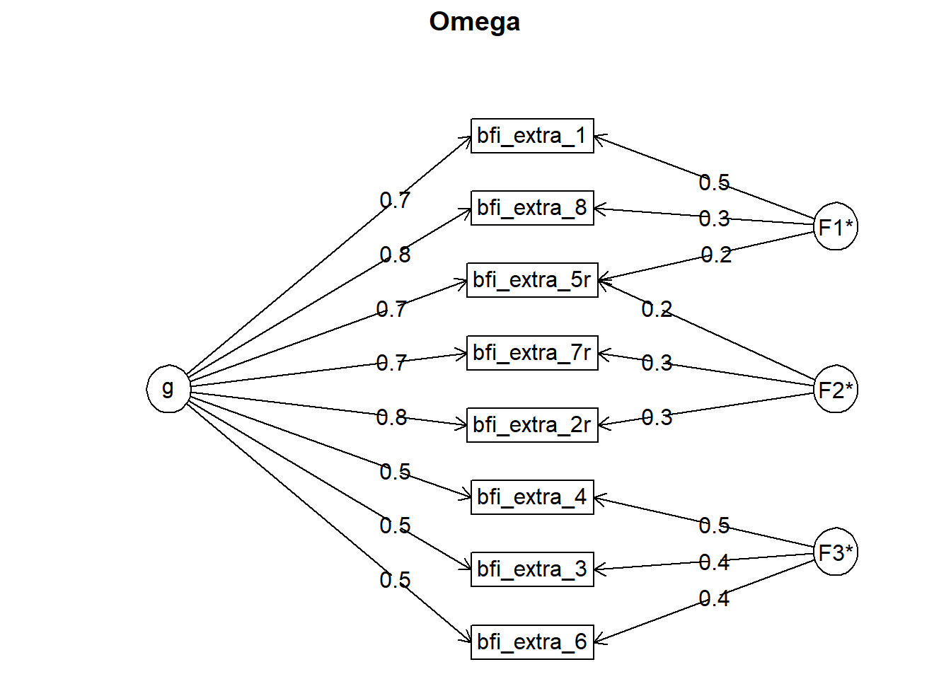

omega_bfi_extra  = data %>%
  select(starts_with("bfi_extra_")) %>%
  psych::omega()

omega_bfi_extra

## Omega 
## Call: omegah(m = m, nfactors = nfactors, fm = fm, key = key, flip = flip, 
##     digits = digits, title = title, sl = sl, labels = labels, 
##     plot = plot, n.obs = n.obs, rotate = rotate, Phi = Phi, option = option, 
##     covar = covar)
## Alpha:                 0.87 
## G.6:                   0.87 
## Omega Hierarchical:    0.77 
## Omega H asymptotic:    0.85 
## Omega Total            0.9 
## 
## Schmid Leiman Factor loadings greater than  0.2 
##                 g   F1*   F2*   F3*   h2   u2   p2
## bfi_extra_1  0.70  0.46             0.71 0.29 0.69
## bfi_extra_3  0.47              0.41 0.39 0.61 0.57
## bfi_extra_2r 0.76        0.29       0.68 0.32 0.86
## bfi_extra_4  0.54              0.46 0.51 0.49 0.57
## bfi_extra_5r 0.74  0.23  0.23       0.65 0.35 0.84
## bfi_extra_6  0.47              0.39 0.39 0.61 0.56
## bfi_extra_7r 0.67        0.34       0.57 0.43 0.79
## bfi_extra_8  0.76  0.30             0.70 0.30 0.83
## 
## With eigenvalues of:
##    g  F1*  F2*  F3* 
## 3.37 0.39 0.28 0.55 
## 
## general/max  6.12   max/min =   1.98
## mean percent general =  0.71    with sd =  0.13 and cv of  0.19 
## Explained Common Variance of the general factor =  0.73 
## 
## The degrees of freedom are 7  and the fit is  0.03 
## The number of observations was  1179  with Chi Square =  40.29  with prob <  0.0000011
## The root mean square of the residuals is  0.01 
## The df corrected root mean square of the residuals is  0.03
## RMSEA index =  0.064  and the 10 % confidence intervals are  0.045 0.083
## BIC =  -9.22
## 
## Compare this with the adequacy of just a general factor and no group factors
## The degrees of freedom for just the general factor are 20  and the fit is  0.33 
## The number of observations was  1179  with Chi Square =  389.9  with prob <  2.6e-70
## The root mean square of the residuals is  0.08 
## The df corrected root mean square of the residuals is  0.1 
## 
## RMSEA index =  0.125  and the 10 % confidence intervals are  0.115 0.136
## BIC =  248.4 
## 
## Measures of factor score adequacy             
##                                                  g   F1*   F2*   F3*
## Correlation of scores with factors            0.89  0.60  0.46  0.64
## Multiple R square of scores with factors      0.79  0.36  0.22  0.41
## Minimum correlation of factor score estimates 0.58 -0.28 -0.57 -0.19
## 
##  Total, General and Subset omega for each subset
##                                                  g  F1*  F2*  F3*
## Omega total for total scores and subscales    0.90 0.84 0.77 0.69
## Omega general for total scores and subscales  0.77 0.70 0.64 0.40
## Omega group for total scores and subscales    0.09 0.14 0.13 0.29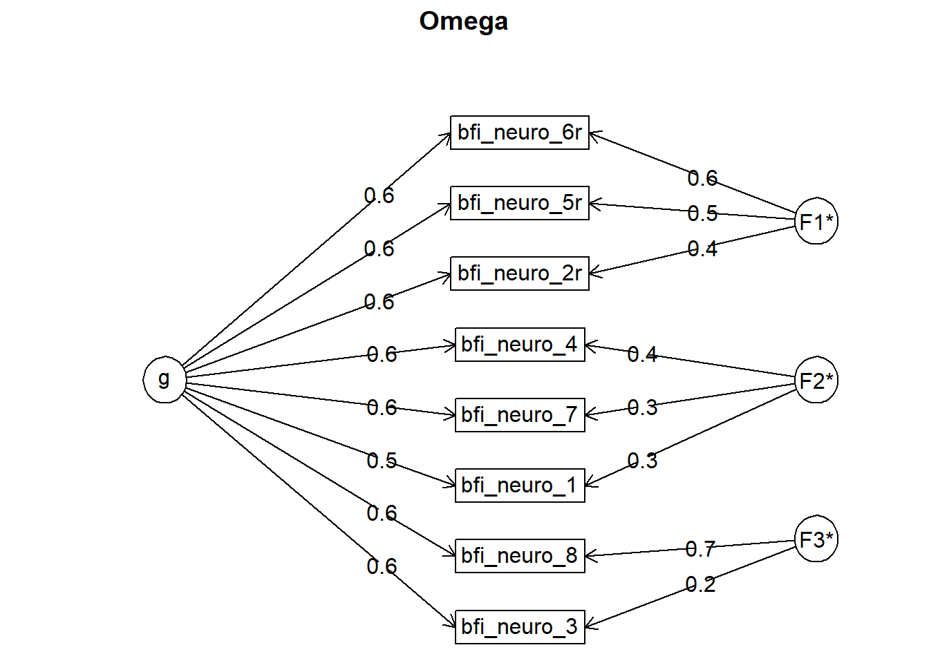

omega_bfi_neuro  = data %>%
  select(starts_with("bfi_neuro_")) %>%
  psych::omega()

omega_bfi_neuro

## Omega 
## Call: omegah(m = m, nfactors = nfactors, fm = fm, key = key, flip = flip, 
##     digits = digits, title = title, sl = sl, labels = labels, 
##     plot = plot, n.obs = n.obs, rotate = rotate, Phi = Phi, option = option, 
##     covar = covar)
## Alpha:                 0.85 
## G.6:                   0.85 
## Omega Hierarchical:    0.71 
## Omega H asymptotic:    0.8 
## Omega Total            0.89 
## 
## Schmid Leiman Factor loadings greater than  0.2 
##                 g   F1*   F2*   F3*   h2   u2   p2
## bfi_neuro_2r 0.61  0.44             0.57 0.43 0.65
## bfi_neuro_1  0.54        0.30       0.41 0.59 0.72
## bfi_neuro_3  0.62              0.22 0.49 0.51 0.79
## bfi_neuro_4  0.57        0.35       0.45 0.55 0.72
## bfi_neuro_5r 0.60  0.46             0.57 0.43 0.63
## bfi_neuro_8  0.60              0.73 0.89 0.11 0.41
## bfi_neuro_6r 0.59  0.57             0.68 0.32 0.52
## bfi_neuro_7  0.59        0.33       0.48 0.52 0.74
## 
## With eigenvalues of:
##    g  F1*  F2*  F3* 
## 2.80 0.78 0.36 0.60 
## 
## general/max  3.6   max/min =   2.16
## mean percent general =  0.65    with sd =  0.13 and cv of  0.2 
## Explained Common Variance of the general factor =  0.62 
## 
## The degrees of freedom are 7  and the fit is  0.02 
## The number of observations was  1179  with Chi Square =  18.32  with prob <  0.011
## The root mean square of the residuals is  0.01 
## The df corrected root mean square of the residuals is  0.02
## RMSEA index =  0.037  and the 10 % confidence intervals are  0.017 0.058
## BIC =  -31.18
## 
## Compare this with the adequacy of just a general factor and no group factors
## The degrees of freedom for just the general factor are 20  and the fit is  0.45 
## The number of observations was  1179  with Chi Square =  526.3  with prob <  8.9e-99
## The root mean square of the residuals is  0.1 
## The df corrected root mean square of the residuals is  0.12 
## 
## RMSEA index =  0.147  and the 10 % confidence intervals are  0.136 0.158
## BIC =  384.9 
## 
## Measures of factor score adequacy             
##                                                  g   F1*   F2*  F3*
## Correlation of scores with factors            0.85  0.70  0.52 0.83
## Multiple R square of scores with factors      0.72  0.49  0.27 0.69
## Minimum correlation of factor score estimates 0.44 -0.03 -0.46 0.39
## 
##  Total, General and Subset omega for each subset
##                                                  g  F1*  F2*  F3*
## Omega total for total scores and subscales    0.89 0.82 0.70 0.78
## Omega general for total scores and subscales  0.71 0.49 0.52 0.49
## Omega group for total scores and subscales    0.13 0.33 0.18 0.29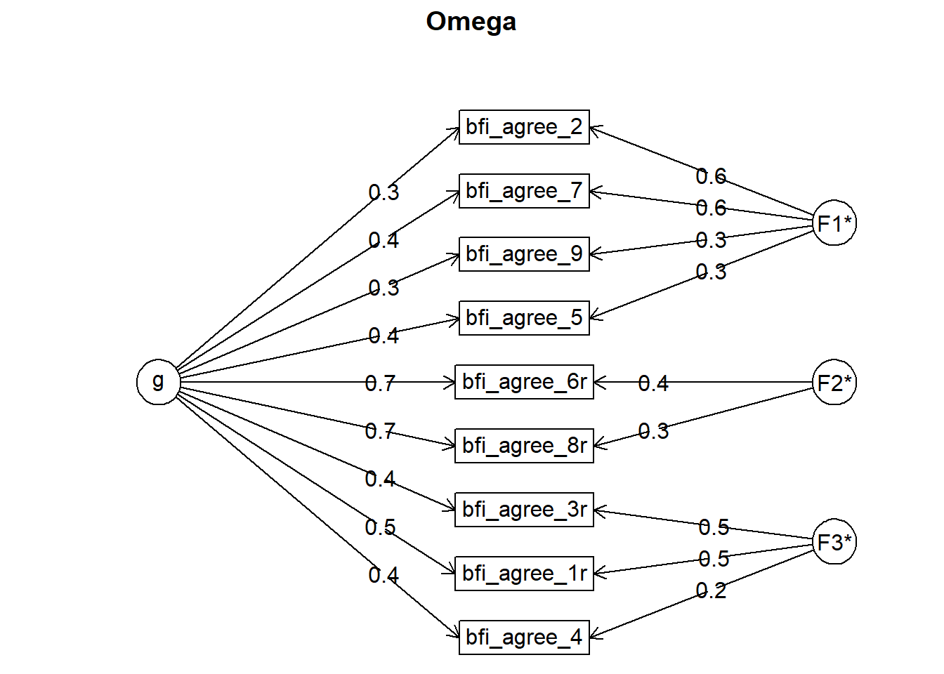

omega_bfi_agree  = data %>%
  select(starts_with("bfi_agree_")) %>%
  psych::omega()

omega_bfi_agree

## Omega 
## Call: omegah(m = m, nfactors = nfactors, fm = fm, key = key, flip = flip, 
##     digits = digits, title = title, sl = sl, labels = labels, 
##     plot = plot, n.obs = n.obs, rotate = rotate, Phi = Phi, option = option, 
##     covar = covar)
## Alpha:                 0.76 
## G.6:                   0.77 
## Omega Hierarchical:    0.57 
## Omega H asymptotic:    0.7 
## Omega Total            0.81 
## 
## Schmid Leiman Factor loadings greater than  0.2 
##                 g   F1*   F2*   F3*   h2   u2   p2
## bfi_agree_2  0.34  0.60             0.48 0.52 0.24
## bfi_agree_3r 0.37              0.51 0.40 0.60 0.35
## bfi_agree_1r 0.45              0.46 0.42 0.58 0.49
## bfi_agree_4  0.35              0.25 0.20 0.80 0.62
## bfi_agree_5  0.36  0.28             0.21 0.79 0.60
## bfi_agree_6r 0.70        0.42       0.68 0.32 0.73
## bfi_agree_7  0.37  0.56             0.46 0.54 0.30
## bfi_agree_8r 0.74        0.35       0.68 0.32 0.79
## bfi_agree_9  0.29  0.31             0.21 0.79 0.40
## 
## With eigenvalues of:
##    g  F1*  F2*  F3* 
## 1.97 0.87 0.31 0.59 
## 
## general/max  2.25   max/min =   2.82
## mean percent general =  0.5    with sd =  0.19 and cv of  0.39 
## Explained Common Variance of the general factor =  0.53 
## 
## The degrees of freedom are 12  and the fit is  0.05 
## The number of observations was  1179  with Chi Square =  62.1  with prob <  0.0000000093
## The root mean square of the residuals is  0.03 
## The df corrected root mean square of the residuals is  0.05
## RMSEA index =  0.06  and the 10 % confidence intervals are  0.045 0.075
## BIC =  -22.77
## 
## Compare this with the adequacy of just a general factor and no group factors
## The degrees of freedom for just the general factor are 27  and the fit is  0.5 
## The number of observations was  1179  with Chi Square =  585.6  with prob <  2.8e-106
## The root mean square of the residuals is  0.11 
## The df corrected root mean square of the residuals is  0.13 
## 
## RMSEA index =  0.132  and the 10 % confidence intervals are  0.123 0.142
## BIC =  394.7 
## 
## Measures of factor score adequacy             
##                                                  g  F1*   F2*   F3*
## Correlation of scores with factors            0.83 0.74  0.49  0.66
## Multiple R square of scores with factors      0.69 0.55  0.24  0.43
## Minimum correlation of factor score estimates 0.37 0.10 -0.53 -0.13
## 
##  Total, General and Subset omega for each subset
##                                                  g  F1*  F2*  F3*
## Omega total for total scores and subscales    0.81 0.65 0.80 0.59
## Omega general for total scores and subscales  0.57 0.24 0.63 0.28
## Omega group for total scores and subscales    0.19 0.41 0.18 0.30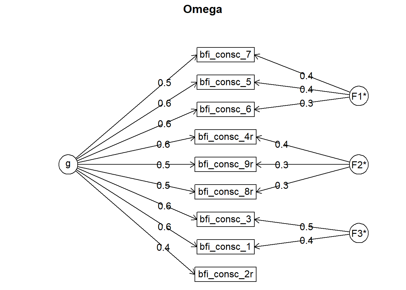

omega_bfi_consc  = data %>%
  select(starts_with("bfi_consc_")) %>%
  psych::omega()

omega_bfi_consc

## Omega 
## Call: omegah(m = m, nfactors = nfactors, fm = fm, key = key, flip = flip, 
##     digits = digits, title = title, sl = sl, labels = labels, 
##     plot = plot, n.obs = n.obs, rotate = rotate, Phi = Phi, option = option, 
##     covar = covar)
## Alpha:                 0.82 
## G.6:                   0.81 
## Omega Hierarchical:    0.7 
## Omega H asymptotic:    0.83 
## Omega Total            0.85 
## 
## Schmid Leiman Factor loadings greater than  0.2 
##                 g   F1*   F2*   F3*   h2   u2   p2
## bfi_consc_2r 0.39                   0.21 0.79 0.70
## bfi_consc_3  0.59              0.49 0.58 0.42 0.59
## bfi_consc_1  0.61              0.35 0.51 0.49 0.73
## bfi_consc_9r 0.52        0.34       0.40 0.60 0.67
## bfi_consc_4r 0.58        0.37       0.48 0.52 0.70
## bfi_consc_5  0.55  0.37             0.45 0.55 0.69
## bfi_consc_6  0.56  0.28             0.40 0.60 0.77
## bfi_consc_7  0.53  0.44             0.47 0.53 0.60
## bfi_consc_8r 0.51        0.25       0.34 0.66 0.76
## 
## With eigenvalues of:
##    g  F1*  F2*  F3* 
## 2.63 0.44 0.36 0.42 
## 
## general/max  6.03   max/min =   1.21
## mean percent general =  0.69    with sd =  0.06 and cv of  0.09 
## Explained Common Variance of the general factor =  0.68 
## 
## The degrees of freedom are 12  and the fit is  0.04 
## The number of observations was  1179  with Chi Square =  47.01  with prob <  0.0000046
## The root mean square of the residuals is  0.02 
## The df corrected root mean square of the residuals is  0.03
## RMSEA index =  0.05  and the 10 % confidence intervals are  0.035 0.065
## BIC =  -37.86
## 
## Compare this with the adequacy of just a general factor and no group factors
## The degrees of freedom for just the general factor are 27  and the fit is  0.24 
## The number of observations was  1179  with Chi Square =  281.4  with prob <  3.6e-44
## The root mean square of the residuals is  0.07 
## The df corrected root mean square of the residuals is  0.08 
## 
## RMSEA index =  0.089  and the 10 % confidence intervals are  0.08 0.099
## BIC =  90.46 
## 
## Measures of factor score adequacy             
##                                                  g   F1*   F2*   F3*
## Correlation of scores with factors            0.84  0.57  0.52  0.59
## Multiple R square of scores with factors      0.71  0.32  0.27  0.35
## Minimum correlation of factor score estimates 0.42 -0.36 -0.46 -0.31
## 
##  Total, General and Subset omega for each subset
##                                                  g  F1*  F2*  F3*
## Omega total for total scores and subscales    0.85 0.70 0.66 0.67
## Omega general for total scores and subscales  0.70 0.49 0.49 0.47
## Omega group for total scores and subscales    0.10 0.21 0.18 0.20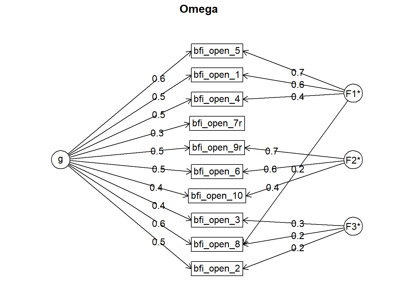

omega_bfi_open  = data %>%
  select(starts_with("bfi_open_")) %>%
  psych::omega()

omega_bfi_open

## Omega 
## Call: omegah(m = m, nfactors = nfactors, fm = fm, key = key, flip = flip, 
##     digits = digits, title = title, sl = sl, labels = labels, 
##     plot = plot, n.obs = n.obs, rotate = rotate, Phi = Phi, option = option, 
##     covar = covar)
## Alpha:                 0.81 
## G.6:                   0.83 
## Omega Hierarchical:    0.63 
## Omega H asymptotic:    0.73 
## Omega Total            0.85 
## 
## Schmid Leiman Factor loadings greater than  0.2 
##                g   F1*   F2*   F3*   h2   u2   p2
## bfi_open_1  0.54  0.57             0.62 0.38 0.46
## bfi_open_2  0.46              0.22 0.27 0.73 0.78
## bfi_open_3  0.44              0.30 0.29 0.71 0.68
## bfi_open_4  0.50  0.35             0.39 0.61 0.64
## bfi_open_5  0.58  0.69             0.81 0.19 0.41
## bfi_open_6  0.49        0.59       0.59 0.41 0.41
## bfi_open_7r 0.25                   0.09 0.91 0.72
## bfi_open_8  0.59  0.22        0.24 0.45 0.55 0.76
## bfi_open_9r 0.52        0.69       0.74 0.26 0.36
## bfi_open_10 0.44        0.42       0.38 0.62 0.52
## 
## With eigenvalues of:
##    g  F1*  F2*  F3* 
## 2.39 1.00 1.01 0.22 
## 
## general/max  2.36   max/min =   4.53
## mean percent general =  0.57    with sd =  0.16 and cv of  0.28 
## Explained Common Variance of the general factor =  0.52 
## 
## The degrees of freedom are 18  and the fit is  0.06 
## The number of observations was  1179  with Chi Square =  67.83  with prob <  0.0000001
## The root mean square of the residuals is  0.02 
## The df corrected root mean square of the residuals is  0.04
## RMSEA index =  0.048  and the 10 % confidence intervals are  0.037 0.061
## BIC =  -59.47
## 
## Compare this with the adequacy of just a general factor and no group factors
## The degrees of freedom for just the general factor are 35  and the fit is  0.98 
## The number of observations was  1179  with Chi Square =  1144  with prob <  1.4e-217
## The root mean square of the residuals is  0.12 
## The df corrected root mean square of the residuals is  0.14 
## 
## RMSEA index =  0.164  and the 10 % confidence intervals are  0.156 0.172
## BIC =  896.5 
## 
## Measures of factor score adequacy             
##                                                  g  F1*  F2*   F3*
## Correlation of scores with factors            0.80 0.77 0.78  0.44
## Multiple R square of scores with factors      0.64 0.60 0.61  0.19
## Minimum correlation of factor score estimates 0.28 0.19 0.22 -0.62
## 
##  Total, General and Subset omega for each subset
##                                                  g  F1*  F2*  F3*
## Omega total for total scores and subscales    0.85 0.76 0.79 0.58
## Omega general for total scores and subscales  0.63 0.41 0.33 0.46
## Omega group for total scores and subscales    0.17 0.35 0.46 0.12

Attractiveness Partner

cronbachs_alpha_attractiveness_partner  = data %>%
  select(starts_with("partner_attractiveness_")) %>%
  filter(!is.na(partner_attractiveness_body)) %>%
  psych::alpha()
cronbachs_alpha_attractiveness_partner

## 
## Reliability analysis   
## Call: psych::alpha(x = .)
## 
##   raw_alpha std.alpha G6(smc) average_r S/N   ase mean   sd median_r
##       0.68      0.68    0.52      0.52 2.2 0.023  4.3 0.74     0.52
## 
##  lower alpha upper     95% confidence boundaries
## 0.63 0.68 0.72 
## 
##  Reliability if an item is dropped:
##                             raw_alpha std.alpha G6(smc) average_r S/N alpha se var.r med.r
## partner_attractiveness_face      0.44      0.52    0.27      0.52 1.1       NA     0  0.52
## partner_attractiveness_body      0.62      0.52    0.27      0.52 1.1       NA     0  0.52
## 
##  Item statistics 
##                               n raw.r std.r r.cor r.drop mean   sd
## partner_attractiveness_face 774  0.85  0.87  0.63   0.52  4.4 0.77
## partner_attractiveness_body 774  0.89  0.87  0.63   0.52  4.1 0.92
## 
## Non missing response frequency for each item
##                                1    2    3    4    5 miss
## partner_attractiveness_face 0.00 0.02 0.10 0.34 0.54    0
## partner_attractiveness_body 0.01 0.07 0.14 0.39 0.40    0

Relationship Satisfaction

cronbachs_alpha_relationship_satisfaction  = data %>%
  select(relationship_satisfaction_overall,
         relationship_satisfaction_2,
         relationship_satisfaction_3,
         relationship_problems_R,
         relationship_conflict_R) %>%
  filter(!is.na(relationship_satisfaction_overall)) %>%
  psych::alpha()
cronbachs_alpha_relationship_satisfaction

## 
## Reliability analysis   
## Call: psych::alpha(x = .)
## 
##   raw_alpha std.alpha G6(smc) average_r S/N    ase mean   sd median_r
##       0.88      0.88    0.88       0.6 7.4 0.0073    4 0.85     0.63
## 
##  lower alpha upper     95% confidence boundaries
## 0.86 0.88 0.89 
## 
##  Reliability if an item is dropped:
##                                   raw_alpha std.alpha G6(smc) average_r S/N alpha se  var.r med.r
## relationship_satisfaction_overall      0.83      0.84    0.82      0.56 5.1   0.0100 0.0150  0.58
## relationship_satisfaction_2            0.85      0.86    0.86      0.60 6.0   0.0090 0.0203  0.63
## relationship_satisfaction_3            0.84      0.84    0.83      0.57 5.3   0.0097 0.0170  0.60
## relationship_problems_R                0.84      0.85    0.83      0.58 5.6   0.0100 0.0317  0.57
## relationship_conflict_R                0.89      0.89    0.87      0.67 8.2   0.0068 0.0075  0.68
## 
##  Item statistics 
##                                     n raw.r std.r r.cor r.drop mean   sd
## relationship_satisfaction_overall 774  0.86  0.88  0.86   0.78  4.3 0.96
## relationship_satisfaction_2       774  0.81  0.82  0.76   0.70  4.0 1.03
## relationship_satisfaction_3       774  0.85  0.86  0.84   0.76  4.2 0.93
## relationship_problems_R           774  0.86  0.84  0.80   0.75  3.9 1.13
## relationship_conflict_R           774  0.73  0.71  0.61   0.56  3.7 1.14
## 
## Non missing response frequency for each item
##                                      1    2    3    4    5 miss
## relationship_satisfaction_overall 0.02 0.04 0.11 0.26 0.56    0
## relationship_satisfaction_2       0.03 0.07 0.15 0.38 0.37    0
## relationship_satisfaction_3       0.01 0.05 0.13 0.32 0.49    0
## relationship_problems_R           0.05 0.08 0.18 0.33 0.36    0
## relationship_conflict_R           0.04 0.13 0.21 0.33 0.29    0

omega_relationship_satisfaction  = data %>%
  select(relationship_satisfaction_overall,
         relationship_satisfaction_2,
         relationship_satisfaction_3,
         relationship_problems_R,
         relationship_conflict_R) %>%
  filter(!is.na(relationship_satisfaction_overall)) %>%
  psych::omega()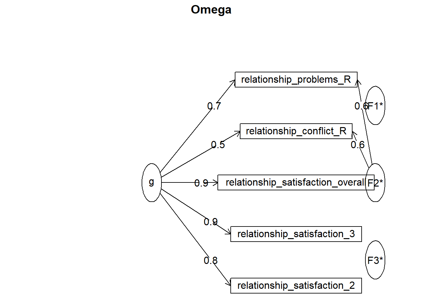

omega_relationship_satisfaction

## Omega 
## Call: omegah(m = m, nfactors = nfactors, fm = fm, key = key, flip = flip, 
##     digits = digits, title = title, sl = sl, labels = labels, 
##     plot = plot, n.obs = n.obs, rotate = rotate, Phi = Phi, option = option, 
##     covar = covar)
## Alpha:                 0.88 
## G.6:                   0.88 
## Omega Hierarchical:    0.83 
## Omega H asymptotic:    0.9 
## Omega Total            0.92 
## 
## Schmid Leiman Factor loadings greater than  0.2 
##                                      g  F1*  F2*  F3*   h2   u2   p2
## relationship_satisfaction_overall 0.92                0.85 0.15 0.99
## relationship_satisfaction_2       0.81                0.64 0.36 1.03
## relationship_satisfaction_3       0.89                0.78 0.22 1.03
## relationship_problems_R           0.67      0.60      0.80 0.20 0.55
## relationship_conflict_R           0.46      0.60      0.61 0.39 0.36
## 
## With eigenvalues of:
##    g  F1*  F2*  F3* 
## 2.96 0.00 0.73 0.04 
## 
## general/max  4.07   max/min =   Inf
## mean percent general =  0.79    with sd =  0.32 and cv of  0.4 
## Explained Common Variance of the general factor =  0.79 
## 
## The degrees of freedom are -2  and the fit is  0 
## The number of observations was  774  with Chi Square =  0  with prob <  NA
## The root mean square of the residuals is  0 
## The df corrected root mean square of the residuals is  NA
## 
## Compare this with the adequacy of just a general factor and no group factors
## The degrees of freedom for just the general factor are 5  and the fit is  0.32 
## The number of observations was  774  with Chi Square =  245.1  with prob <  6.1e-51
## The root mean square of the residuals is  0.11 
## The df corrected root mean square of the residuals is  0.16 
## 
## RMSEA index =  0.249  and the 10 % confidence intervals are  0.223 0.276
## BIC =  211.9 
## 
## Measures of factor score adequacy             
##                                                  g F1*  F2*   F3*
## Correlation of scores with factors            0.97   0 0.85  0.39
## Multiple R square of scores with factors      0.93   0 0.73  0.15
## Minimum correlation of factor score estimates 0.87  -1 0.46 -0.69
## 
##  Total, General and Subset omega for each subset
##                                                  g F1*  F2*  F3*
## Omega total for total scores and subscales    0.92  NA 0.82 0.92
## Omega general for total scores and subscales  0.83  NA 0.38 0.92
## Omega group for total scores and subscales    0.09  NA 0.44 0.00

Reliabilities

reliability = data.frame(x = 1:7) %>%
  cbind(Variable = c("bfi_extra", "bfi_neuro", "bfi_agree", "bfi_consc", "bfi_open",
                  "attractiveness_partner", "relationship_satisfaction"),
        alpha = c(cronbachs_alpha_bfi_extra$total$std.alpha,
                  cronbachs_alpha_bfi_neuro$total$std.alpha,
                  cronbachs_alpha_bfi_agree$total$std.alpha,
                  cronbachs_alpha_bfi_consc$total$std.alpha,
                  cronbachs_alpha_bfi_open$total$std.alpha,
                  cronbachs_alpha_attractiveness_partner$total$std.alpha,
                  cronbachs_alpha_relationship_satisfaction$total$std.alpha),
        omega_h = c(omega_bfi_extra$omega_h,
                  omega_bfi_neuro$omega_h,
                  omega_bfi_agree$omega_h,
                  omega_bfi_consc$omega_h,
                  omega_bfi_open$omega_h,
                  NA,
                  omega_relationship_satisfaction$omega_h)) %>%
  mutate(alpha = round(alpha, 2),
         omega_h = round(omega_h, 2)) %>%
  select(-x)

kable(reliability)

Variable	alpha	omega_h
bfi_extra	0.87	0.77
bfi_neuro	0.85	0.71
bfi_agree	0.76	0.57
bfi_consc	0.82	0.70
bfi_open	0.81	0.63
attractiveness_partner	0.68	NA
relationship_satisfaction	0.88	0.83

Summary

Means, sds, ranges, and reliability estimeate

summary = left_join(mean_sd_range, reliability, by = "Variable")
kable(summary)

Variable	n	mean	sd	min	max	alpha	omega_h
age	1179	25.03	5.09	18.00	49.00	NA	NA
education_years	1179	15.07	4.73	0.00	26.00	NA	NA
net_income	NA	NA	NA	NA	NA	NA	NA
bfi_extra	1179	3.46	0.78	1.12	5.00	0.87	0.77
bfi_neuro	1179	3.00	0.78	1.00	5.00	0.85	0.71
bfi_agree	1179	3.68	0.62	1.44	5.00	0.76	0.57
bfi_consc	1179	3.53	0.66	1.56	5.00	0.82	0.70
bfi_open	1179	3.78	0.61	1.50	5.00	0.81	0.63
religiosity	1179	2.20	1.34	1.00	6.00	NA	NA
relationship_duration	NA	NA	NA	NA	NA	NA	NA
attractiveness_partner	774	4.25	0.74	1.00	5.00	0.68	NA
relationship_satisfaction	774	3.39	0.43	1.40	4.60	0.88	0.83
satisfaction_sexual_intercourse	774	4.00	1.05	1.00	5.00	NA	NA
diary_libido_mean	968	1.19	0.59	0.00	3.03	NA	NA
diary_sex_active_sex_sum	897	7.27	7.19	0.00	42.00	NA	NA
diary_masturbation_sum	897	6.96	7.21	0.00	50.00	NA	NA

Zero-Order Correlations

library(apaTables)

correlations = data %>%
  select(age, education_years,
         bfi_extra, bfi_neuro, bfi_agree, bfi_consc, bfi_open,
         religiosity,
         attractiveness_partner, 
         relationship_satisfaction, 
         satisfaction_sexual_intercourse,
         diary_libido_mean, diary_masturbation_sum, diary_sex_active_sex_sum)

correlations_table = apa.cor.table(correlations, filename = "Table.doc", table.number = 4)

correlations_table

## 
## 
## Table 4 
## 
## Means, standard deviations, and correlations with confidence intervals
##  
## 
##   Variable                            M     SD   1            2            3            4           
##   1. age                              25.03 5.09                                                    
##                                                                                                     
##   2. education_years                  15.07 4.73 .36**                                              
##                                                  [.31, .41]                                         
##                                                                                                     
##   3. bfi_extra                        3.46  0.78 -.03         -.06*                                 
##                                                  [-.08, .03]  [-.11, -.00]                          
##                                                                                                     
##   4. bfi_neuro                        3.00  0.78 -.02         .03          -.36**                   
##                                                  [-.08, .03]  [-.03, .08]  [-.40, -.30]             
##                                                                                                     
##   5. bfi_agree                        3.68  0.62 -.10**       -.09**       .21**        -.39**      
##                                                  [-.16, -.05] [-.14, -.03] [.16, .27]   [-.44, -.34]
##                                                                                                     
##   6. bfi_consc                        3.53  0.66 -.03         -.05         .21**        -.26**      
##                                                  [-.09, .03]  [-.11, .01]  [.16, .27]   [-.32, -.21]
##                                                                                                     
##   7. bfi_open                         3.78  0.61 .10**        .08**        .20**        -.07*       
##                                                  [.04, .16]   [.03, .14]   [.14, .25]   [-.13, -.01]
##                                                                                                     
##   8. religiosity                      2.20  1.34 -.05         .01          .06*         -.05        
##                                                  [-.10, .01]  [-.04, .07]  [.00, .12]   [-.10, .01] 
##                                                                                                     
##   9. attractiveness_partner           4.25  0.74 -.03         .02          .09*         -.05        
##                                                  [-.10, .04]  [-.05, .09]  [.02, .16]   [-.12, .02] 
##                                                                                                     
##   10. relationship_satisfaction       3.39  0.43 -.11**       -.07         .03          .06         
##                                                  [-.17, -.03] [-.14, .00]  [-.04, .10]  [-.01, .13] 
##                                                                                                     
##   11. satisfaction_sexual_intercourse 4.00  1.05 -.06         -.05         .12**        -.13**      
##                                                  [-.13, .01]  [-.12, .02]  [.05, .19]   [-.19, -.06]
##                                                                                                     
##   12. diary_libido_mean               1.19  0.59 .07*         .03          .15**        -.07*       
##                                                  [.01, .13]   [-.03, .09]  [.08, .21]   [-.13, -.01]
##                                                                                                     
##   13. diary_masturbation_sum          6.96  7.21 .02          .02          -.01         -.00        
##                                                  [-.04, .09]  [-.04, .09]  [-.07, .06]  [-.07, .06] 
##                                                                                                     
##   14. diary_sex_active_sex_sum        7.27  7.19 .03          -.01         .02          -.04        
##                                                  [-.03, .10]  [-.08, .05]  [-.05, .08]  [-.10, .03] 
##                                                                                                     
##   5           6            7           8            9            10           11           12        
##                                                                                                      
##                                                                                                      
##                                                                                                      
##                                                                                                      
##                                                                                                      
##                                                                                                      
##                                                                                                      
##                                                                                                      
##                                                                                                      
##                                                                                                      
##                                                                                                      
##                                                                                                      
##                                                                                                      
##                                                                                                      
##   .20**                                                                                              
##   [.14, .25]                                                                                         
##                                                                                                      
##   .08**       .05                                                                                    
##   [.02, .13]  [-.01, .11]                                                                            
##                                                                                                      
##   .10**       .08**        .01                                                                       
##   [.04, .16]  [.02, .14]   [-.05, .07]                                                               
##                                                                                                      
##   .10**       .06          .07*        .01                                                           
##   [.03, .17]  [-.01, .13]  [.00, .14]  [-.06, .08]                                                   
##                                                                                                      
##   -.03        .02          -.04        .10**        .25**                                            
##   [-.10, .04] [-.05, .09]  [-.11, .03] [.03, .17]   [.19, .32]                                       
##                                                                                                      
##   .12**       .12**        -.02        .01          .41**        .33**                               
##   [.05, .19]  [.05, .19]   [-.09, .05] [-.06, .08]  [.35, .47]   [.27, .39]                          
##                                                                                                      
##   .09**       -.05         .13**       -.01         .09*         .03          .14**                  
##   [.02, .15]  [-.11, .02]  [.07, .19]  [-.07, .05]  [.01, .16]   [-.05, .11]  [.06, .21]             
##                                                                                                      
##   -.01        -.12**       .13**       -.10**       -.10**       -.19**       -.11**       .22**     
##   [-.08, .05] [-.19, -.06] [.06, .19]  [-.16, -.03] [-.18, -.03] [-.27, -.12] [-.19, -.03] [.16, .29]
##                                                                                                      
##   .05         .09**        -.01        .01          .13**        .13**        .23**        .39**     
##   [-.01, .12] [.02, .15]   [-.08, .05] [-.05, .08]  [.05, .20]   [.05, .21]   [.16, .31]   [.34, .45]
##                                                                                                      
##   13         
##              
##              
##              
##              
##              
##              
##              
##              
##              
##              
##              
##              
##              
##              
##              
##              
##              
##              
##              
##              
##              
##              
##              
##              
##              
##              
##              
##              
##              
##              
##              
##              
##              
##              
##              
##              
##              
##              
##   -.05       
##   [-.11, .02]
##              
## 
## Note. M and SD are used to represent mean and standard deviation, respectively.
## Values in square brackets indicate the 95% confidence interval.
## The confidence interval is a plausible range of population correlations 
## that could have caused the sample correlation (Cumming, 2014).
##  * indicates p < .05. ** indicates p < .01.
##

Means and sds by contraceptive group

means_sd_congroup = data %>%
  group_by(contraception_hormonal, congruent_contraception) %>%
  summarize(count = n(),
            count_diary = sum(!is.na(diary_libido_mean)),
            age_mean = round(mean(age, na.rm = T), 2),
            age_sd = round(sd(age, na.rm = T), 2),
            education_years_mean = round(mean(education_years, na.rm = T), 2),
            education_years_sd = round(sd(education_years, na.rm = T), 2),
            bfi_extra_mean = round(mean(bfi_extra, na.rm = T), 2),
            bfi_extra_sd = round(sd(bfi_extra, na.rm = T), 2),
            bfi_neuro_mean = round(mean(bfi_neuro, na.rm = T), 2),
            bfi_neuro_sd = round(sd(bfi_neuro, na.rm = T), 2),
            bfi_agree_mean = round(mean(bfi_agree, na.rm = T), 2),
            bfi_agree_sd = round(sd(bfi_agree, na.rm = T), 2),
            bfi_consc_mean = round(mean(bfi_consc, na.rm = T), 2),
            bfi_consc_sd = round(sd(bfi_consc, na.rm = T), 2),
            bfi_open_mean = round(mean(bfi_open, na.rm = T), 2),
            bfi_open_sd = round(sd(bfi_open, na.rm = T), 2),
            religiosity_mean = round(mean(religiosity, na.rm = T), 2),
            religiosity_sd = round(sd(religiosity, na.rm = T), 2),
            attractiveness_partner_mean = round(mean(attractiveness_partner,
                                                     na.rm = T), 2),
            attractiveness_partner_sd = round(sd(attractiveness_partner,
                                                 na.rm = T), 2),
            relationship_satisfaction_mean = round(mean(relationship_satisfaction,
                                                     na.rm = T), 2),
            relationship_satisfaction_sd = round(sd(relationship_satisfaction,
                                                 na.rm = T), 2),
            satisfaction_sexual_intercourse_mean = round(
              mean(satisfaction_sexual_intercourse, na.rm = T), 2),
            satisfaction_sexual_intercourse_sd = round(
              sd(satisfaction_sexual_intercourse, na.rm = T), 2),
            diary_libido_mean_mean = round(mean(diary_libido_mean,
                                                     na.rm = T), 2),
            diary_libido_mean_sd = round(sd(diary_libido_mean,
                                                 na.rm = T), 2),
            diary_sex_active_sex_sum_mean = round(mean(diary_sex_active_sex_sum,
                                                     na.rm = T), 2),
            diary_sex_active_sex_sum_sd = round(sd(diary_sex_active_sex_sum,
                                                 na.rm = T), 2),
            diary_masturbation_sum_mean = round(mean(diary_masturbation_sum,
                                                     na.rm = T), 2),
            diary_masturbation_sum_sd = round(sd(diary_masturbation_sum,
                                                 na.rm = T), 2))

kable(means_sd_congroup)

contraception_hormonal	congruent_contraception	count	count_diary	age_mean	age_sd	education_years_mean	education_years_sd	bfi_extra_mean	bfi_extra_sd	bfi_neuro_mean	bfi_neuro_sd	bfi_agree_mean	bfi_agree_sd	bfi_consc_mean	bfi_consc_sd	bfi_open_mean	bfi_open_sd	religiosity_mean	religiosity_sd	attractiveness_partner_mean	attractiveness_partner_sd	relationship_satisfaction_mean	relationship_satisfaction_sd	satisfaction_sexual_intercourse_mean	satisfaction_sexual_intercourse_sd	diary_libido_mean_mean	diary_libido_mean_sd	diary_sex_active_sex_sum_mean	diary_sex_active_sex_sum_sd	diary_masturbation_sum_mean	diary_masturbation_sum_sd
no	0	150	126	27.01	5.64	15.15	5.07	3.46	0.75	2.97	0.79	3.59	0.60	3.49	0.73	3.77	0.66	2.16	1.29	4.13	0.74	3.42	0.44	3.84	1.12	1.24	0.57	8.02	6.15	6.50	6.50
no	1	251	216	26.59	5.51	16.04	4.71	3.44	0.80	3.03	0.77	3.66	0.60	3.48	0.64	3.87	0.57	2.24	1.37	4.26	0.75	3.31	0.46	3.99	1.05	1.32	0.52	9.15	7.53	7.56	7.88
no	NA	287	247	24.19	4.63	14.39	5.25	3.45	0.74	2.96	0.76	3.68	0.60	3.45	0.63	3.84	0.60	2.22	1.33	NaN	NA	NaN	NA	NaN	NA	1.02	0.64	2.89	4.48	10.06	8.65
yes	0	133	103	23.81	4.17	15.57	4.17	3.46	0.78	3.01	0.80	3.80	0.62	3.58	0.65	3.73	0.60	2.47	1.47	4.29	0.71	3.47	0.38	4.02	1.06	1.24	0.54	10.02	8.13	4.61	5.45
yes	1	240	187	24.33	4.89	14.79	4.21	3.47	0.82	3.02	0.77	3.66	0.66	3.67	0.63	3.63	0.63	2.12	1.31	4.30	0.73	3.42	0.39	4.10	1.00	1.29	0.56	9.61	7.30	4.96	5.37
yes	NA	118	89	24.01	4.34	14.53	4.30	3.55	0.82	2.98	0.84	3.68	0.59	3.54	0.67	3.84	0.58	2.03	1.24	NaN	NA	NaN	NA	NaN	NA	0.97	0.61	2.83	4.27	6.66	6.00

crosstabs(~ relationship_duration_factor + congruent_contraception + contraception_hormonal,
          data = data)

## , , contraception_hormonal = no
## 
##                             congruent_contraception
## relationship_duration_factor   0   1
##   Single                       0   0
##   Partnered_upto12months      13 100
##   Partnered_upto28months      30  66
##   Partnered_upto52months      51  45
##   Partnered_morethan52months  56  40
## 
## , , contraception_hormonal = yes
## 
##                             congruent_contraception
## relationship_duration_factor   0   1
##   Single                       0   0
##   Partnered_upto12months      22  63
##   Partnered_upto28months      31  71
##   Partnered_upto52months      43  49
##   Partnered_morethan52months  37  57

LS0tDQp0aXRsZTogIkRlc2NyaXB0aXZlcyINCm91dHB1dDoNCiAgaHRtbF9kb2N1bWVudDoNCiAgICB0b2M6IHRydWUNCiAgICB0b2NfZGVwdGg6IDQNCiAgICB0b2NfZmxvYXQ6IHRydWUNCiAgICBjb2RlX2ZvbGRpbmc6ICdoaWRlJw0KICAgIHNlbGZfY29udGFpbmVkOiBmYWxzZQ0KLS0tDQoNCg0KIyMgRGF0YSBhbmQgRnVuY3Rpb25zDQpgYGB7ciBkYXRhIGFuZCBmdW5jdGlvbiwgcmVzdWx0cz0naGlkZScsbWVzc2FnZT1GLHdhcm5pbmc9Rn0NCnNvdXJjZSgiMF9oZWxwZXJzLlIiKQ0Ka25pdHI6Om9wdHNfY2h1bmskc2V0KHdhcm5pbmcgPSBGQUxTRSwgbWVzc2FnZSA9IEZBTFNFKQ0KcGFuZGVyOjpwYW5kZXJPcHRpb25zKCJ0YWJsZS5zcGxpdC50YWJsZSIsIEluZikNCnBhbmRlcjo6cGFuZGVyT3B0aW9ucygncm91bmQnLDIpDQpwYW5kZXI6OnBhbmRlck9wdGlvbnMoJ2RpZ2l0cycsMikNCnBhbmRlcjo6cGFuZGVyT3B0aW9ucygna2VlcC50cmFpbGluZy56ZXJvcycsVFJVRSkNCg0KbG9hZCgiZGF0YS9jbGVhbmVkX3NlbGVjdGVkX3dyYW5nbGVkLnJkYXRhIikNCmBgYA0KDQoNCiMjIE1lYW5zLCBTdGFuZGFyZCBEZXZpYXRpb25zIGFuZCBSYW5nZXMNCmBgYHtyfQ0KbWVhbl9zZF9yYW5nZTEgPSBkYXRhICU+JQ0KICBzZWxlY3Qoc2Vzc2lvbiwNCiAgICAgICAgIGFnZSwgZWR1Y2F0aW9uX3llYXJzLA0KICAgICAgICAgYmZpX2V4dHJhLCBiZmlfbmV1cm8sIGJmaV9hZ3JlZSwgYmZpX2NvbnNjLCBiZmlfb3BlbiwNCiAgICAgICAgIHJlbGlnaW9zaXR5LA0KICAgICAgICAgZGlhcnlfbGliaWRvX21lYW4sIGRpYXJ5X21hc3R1cmJhdGlvbl9zdW0sIGRpYXJ5X3NleF9hY3RpdmVfc2V4X3N1bSkgJT4lDQogIHBpdm90X2xvbmdlcigtc2Vzc2lvbiwgbmFtZXNfdG8gPSAiVmFyaWFibGUiLCB2YWx1ZXNfdG8gPSAiVmFsdWUiKSAlPiUNCiAgZ3JvdXBfYnkoVmFyaWFibGUpICU+JQ0KICBzdW1tYXJpc2UobiA9IHN1bSghaXMubmEoVmFsdWUpKSwNCiAgICAgICAgICAgIG1lYW4gPSByb3VuZChtZWFuKFZhbHVlLCBuYS5ybSA9IFQpLCAyKSwNCiAgICAgICAgICAgIHNkID0gcm91bmQoc2QoVmFsdWUsIG5hLnJtID0gVCksIDIpLA0KICAgICAgICAgICAgbWluID0gcm91bmQobWluKFZhbHVlLCBuYS5ybSA9IFQpLCAyKSwNCiAgICAgICAgICAgIG1heCA9IHJvdW5kKG1heChWYWx1ZSwgbmEucm0gPSBUKSwgMikpDQoNCg0KbWVhbl9zZF9yYW5nZTIgPSBkYXRhICU+JQ0KICBzZWxlY3Qoc2Vzc2lvbiwNCiAgICAgICAgIGF0dHJhY3RpdmVuZXNzX3BhcnRuZXIsIA0KICAgICAgICAgcmVsYXRpb25zaGlwX3NhdGlzZmFjdGlvbiwgDQogICAgICAgICBzYXRpc2ZhY3Rpb25fc2V4dWFsX2ludGVyY291cnNlLA0KICAgICAgICAgKSAlPiUNCiAgcGl2b3RfbG9uZ2VyKC1zZXNzaW9uLCBuYW1lc190byA9ICJWYXJpYWJsZSIsIHZhbHVlc190byA9ICJWYWx1ZSIpICU+JQ0KICBncm91cF9ieShWYXJpYWJsZSkgJT4lDQogIHN1bW1hcmlzZShuID0gc3VtKCFpcy5uYShWYWx1ZSkpLA0KICAgICAgICAgICAgbWVhbiA9IHJvdW5kKG1lYW4oVmFsdWUsIG5hLnJtID0gVCksIDIpLA0KICAgICAgICAgICAgc2QgPSByb3VuZChzZChWYWx1ZSwgbmEucm0gPSBUKSwgMiksDQogICAgICAgICAgICBtaW4gPSByb3VuZChtaW4oVmFsdWUsIG5hLnJtID0gVCksIDIpLA0KICAgICAgICAgICAgbWF4ID0gcm91bmQobWF4KFZhbHVlLCBuYS5ybSA9IFQpLCAyKSkNCg0KDQptZWFuX3NkX3JhbmdlID0gZGF0YS5mcmFtZSh4ID0gYygxOjE2KSkgJT4lDQogIGNiaW5kKFZhcmlhYmxlID0gYygiYWdlIiwgImVkdWNhdGlvbl95ZWFycyIsICJuZXRfaW5jb21lIiwgImJmaV9leHRyYSIsICJiZmlfbmV1cm8iLCAiYmZpX2FncmVlIiwgImJmaV9jb25zYyIsICJiZmlfb3BlbiIsICJyZWxpZ2lvc2l0eSIsICJyZWxhdGlvbnNoaXBfZHVyYXRpb24iLCAiYXR0cmFjdGl2ZW5lc3NfcGFydG5lciIsICJyZWxhdGlvbnNoaXBfc2F0aXNmYWN0aW9uIiwgInNhdGlzZmFjdGlvbl9zZXh1YWxfaW50ZXJjb3Vyc2UiLCJkaWFyeV9saWJpZG9fbWVhbiIsICJkaWFyeV9zZXhfYWN0aXZlX3NleF9zdW0iLCAiZGlhcnlfbWFzdHVyYmF0aW9uX3N1bSIpKSAlPiUNCiAgc2VsZWN0KC14KQ0KDQoNCg0KbWVhbl9zZF9yYW5nZSA9IGxlZnRfam9pbihtZWFuX3NkX3JhbmdlLA0KICAgICAgICAgICAgICAgICAgICAgICAgICByYmluZChtZWFuX3NkX3JhbmdlMSwgbWVhbl9zZF9yYW5nZTIpLA0KICAgICAgICAgICAgICAgICAgICAgICAgICBieSA9ICJWYXJpYWJsZSIpDQogICAgICAgICAgICAgICAgICAgICAgICAgICAgDQogICAgICAgICAgICAgICAgICAgICAgICAgICAgDQogICAgICAgICAgICAgICAgICAgICAgICAgICAgDQogIA0Ka2FibGUobWVhbl9zZF9yYW5nZSkNCmBgYA0KDQojIyBSZWxpYWJpbGl0eSB7LnRhYnNldH0NCiMjIyBCaWcgRml2ZSBQZXJzb25hbGl0eQ0KYGBge3J9DQpjcm9uYmFjaHNfYWxwaGFfYmZpX2V4dHJhICA9IGRhdGEgJT4lDQogIHNlbGVjdChzdGFydHNfd2l0aCgiYmZpX2V4dHJhXyIpKSAlPiUNCiAgcHN5Y2g6OmFscGhhKCkNCmNyb25iYWNoc19hbHBoYV9iZmlfZXh0cmENCg0KY3JvbmJhY2hzX2FscGhhX2JmaV9uZXVybyAgPSBkYXRhICU+JQ0KICBzZWxlY3Qoc3RhcnRzX3dpdGgoImJmaV9uZXVyb18iKSkgJT4lDQogIHBzeWNoOjphbHBoYSgpDQpjcm9uYmFjaHNfYWxwaGFfYmZpX25ldXJvDQoNCmNyb25iYWNoc19hbHBoYV9iZmlfYWdyZWUgID0gZGF0YSAlPiUNCiAgc2VsZWN0KHN0YXJ0c193aXRoKCJiZmlfYWdyZWVfIikpICU+JQ0KICBwc3ljaDo6YWxwaGEoKQ0KY3JvbmJhY2hzX2FscGhhX2JmaV9hZ3JlZQ0KDQpjcm9uYmFjaHNfYWxwaGFfYmZpX2NvbnNjICA9IGRhdGEgJT4lDQogIHNlbGVjdChzdGFydHNfd2l0aCgiYmZpX2NvbnNjXyIpKSAlPiUNCiAgcHN5Y2g6OmFscGhhKCkNCmNyb25iYWNoc19hbHBoYV9iZmlfY29uc2MNCg0KY3JvbmJhY2hzX2FscGhhX2JmaV9vcGVuICA9IGRhdGEgJT4lDQogIHNlbGVjdChzdGFydHNfd2l0aCgiYmZpX29wZW5fIikpICU+JQ0KICBwc3ljaDo6YWxwaGEoKQ0KY3JvbmJhY2hzX2FscGhhX2JmaV9vcGVuDQoNCm9tZWdhX2JmaV9leHRyYSAgPSBkYXRhICU+JQ0KICBzZWxlY3Qoc3RhcnRzX3dpdGgoImJmaV9leHRyYV8iKSkgJT4lDQogIHBzeWNoOjpvbWVnYSgpDQpvbWVnYV9iZmlfZXh0cmENCg0Kb21lZ2FfYmZpX25ldXJvICA9IGRhdGEgJT4lDQogIHNlbGVjdChzdGFydHNfd2l0aCgiYmZpX25ldXJvXyIpKSAlPiUNCiAgcHN5Y2g6Om9tZWdhKCkNCm9tZWdhX2JmaV9uZXVybw0KDQpvbWVnYV9iZmlfYWdyZWUgID0gZGF0YSAlPiUNCiAgc2VsZWN0KHN0YXJ0c193aXRoKCJiZmlfYWdyZWVfIikpICU+JQ0KICBwc3ljaDo6b21lZ2EoKQ0Kb21lZ2FfYmZpX2FncmVlDQoNCm9tZWdhX2JmaV9jb25zYyAgPSBkYXRhICU+JQ0KICBzZWxlY3Qoc3RhcnRzX3dpdGgoImJmaV9jb25zY18iKSkgJT4lDQogIHBzeWNoOjpvbWVnYSgpDQpvbWVnYV9iZmlfY29uc2MNCg0Kb21lZ2FfYmZpX29wZW4gID0gZGF0YSAlPiUNCiAgc2VsZWN0KHN0YXJ0c193aXRoKCJiZmlfb3Blbl8iKSkgJT4lDQogIHBzeWNoOjpvbWVnYSgpDQpvbWVnYV9iZmlfb3Blbg0KYGBgDQoNCiMjIyBBdHRyYWN0aXZlbmVzcyBQYXJ0bmVyDQpgYGB7cn0NCmNyb25iYWNoc19hbHBoYV9hdHRyYWN0aXZlbmVzc19wYXJ0bmVyICA9IGRhdGEgJT4lDQogIHNlbGVjdChzdGFydHNfd2l0aCgicGFydG5lcl9hdHRyYWN0aXZlbmVzc18iKSkgJT4lDQogIGZpbHRlcighaXMubmEocGFydG5lcl9hdHRyYWN0aXZlbmVzc19ib2R5KSkgJT4lDQogIHBzeWNoOjphbHBoYSgpDQpjcm9uYmFjaHNfYWxwaGFfYXR0cmFjdGl2ZW5lc3NfcGFydG5lcg0KYGBgDQoNCg0KIyMjIFJlbGF0aW9uc2hpcCBTYXRpc2ZhY3Rpb24NCmBgYHtyfQ0KY3JvbmJhY2hzX2FscGhhX3JlbGF0aW9uc2hpcF9zYXRpc2ZhY3Rpb24gID0gZGF0YSAlPiUNCiAgc2VsZWN0KHJlbGF0aW9uc2hpcF9zYXRpc2ZhY3Rpb25fb3ZlcmFsbCwNCiAgICAgICAgIHJlbGF0aW9uc2hpcF9zYXRpc2ZhY3Rpb25fMiwNCiAgICAgICAgIHJlbGF0aW9uc2hpcF9zYXRpc2ZhY3Rpb25fMywNCiAgICAgICAgIHJlbGF0aW9uc2hpcF9wcm9ibGVtc19SLA0KICAgICAgICAgcmVsYXRpb25zaGlwX2NvbmZsaWN0X1IpICU+JQ0KICBmaWx0ZXIoIWlzLm5hKHJlbGF0aW9uc2hpcF9zYXRpc2ZhY3Rpb25fb3ZlcmFsbCkpICU+JQ0KICBwc3ljaDo6YWxwaGEoKQ0KY3JvbmJhY2hzX2FscGhhX3JlbGF0aW9uc2hpcF9zYXRpc2ZhY3Rpb24NCg0Kb21lZ2FfcmVsYXRpb25zaGlwX3NhdGlzZmFjdGlvbiAgPSBkYXRhICU+JQ0KICBzZWxlY3QocmVsYXRpb25zaGlwX3NhdGlzZmFjdGlvbl9vdmVyYWxsLA0KICAgICAgICAgcmVsYXRpb25zaGlwX3NhdGlzZmFjdGlvbl8yLA0KICAgICAgICAgcmVsYXRpb25zaGlwX3NhdGlzZmFjdGlvbl8zLA0KICAgICAgICAgcmVsYXRpb25zaGlwX3Byb2JsZW1zX1IsDQogICAgICAgICByZWxhdGlvbnNoaXBfY29uZmxpY3RfUikgJT4lDQogIGZpbHRlcighaXMubmEocmVsYXRpb25zaGlwX3NhdGlzZmFjdGlvbl9vdmVyYWxsKSkgJT4lDQogIHBzeWNoOjpvbWVnYSgpDQpvbWVnYV9yZWxhdGlvbnNoaXBfc2F0aXNmYWN0aW9uDQpgYGANCg0KIyMjIFJlbGlhYmlsaXRpZXMgey5hY3RpdmV9DQpgYGB7cn0NCnJlbGlhYmlsaXR5ID0gZGF0YS5mcmFtZSh4ID0gMTo3KSAlPiUNCiAgY2JpbmQoVmFyaWFibGUgPSBjKCJiZmlfZXh0cmEiLCAiYmZpX25ldXJvIiwgImJmaV9hZ3JlZSIsICJiZmlfY29uc2MiLCAiYmZpX29wZW4iLA0KICAgICAgICAgICAgICAgICAgImF0dHJhY3RpdmVuZXNzX3BhcnRuZXIiLCAicmVsYXRpb25zaGlwX3NhdGlzZmFjdGlvbiIpLA0KICAgICAgICBhbHBoYSA9IGMoY3JvbmJhY2hzX2FscGhhX2JmaV9leHRyYSR0b3RhbCRzdGQuYWxwaGEsDQogICAgICAgICAgICAgICAgICBjcm9uYmFjaHNfYWxwaGFfYmZpX25ldXJvJHRvdGFsJHN0ZC5hbHBoYSwNCiAgICAgICAgICAgICAgICAgIGNyb25iYWNoc19hbHBoYV9iZmlfYWdyZWUkdG90YWwkc3RkLmFscGhhLA0KICAgICAgICAgICAgICAgICAgY3JvbmJhY2hzX2FscGhhX2JmaV9jb25zYyR0b3RhbCRzdGQuYWxwaGEsDQogICAgICAgICAgICAgICAgICBjcm9uYmFjaHNfYWxwaGFfYmZpX29wZW4kdG90YWwkc3RkLmFscGhhLA0KICAgICAgICAgICAgICAgICAgY3JvbmJhY2hzX2FscGhhX2F0dHJhY3RpdmVuZXNzX3BhcnRuZXIkdG90YWwkc3RkLmFscGhhLA0KICAgICAgICAgICAgICAgICAgY3JvbmJhY2hzX2FscGhhX3JlbGF0aW9uc2hpcF9zYXRpc2ZhY3Rpb24kdG90YWwkc3RkLmFscGhhKSwNCiAgICAgICAgb21lZ2FfaCA9IGMob21lZ2FfYmZpX2V4dHJhJG9tZWdhX2gsDQogICAgICAgICAgICAgICAgICBvbWVnYV9iZmlfbmV1cm8kb21lZ2FfaCwNCiAgICAgICAgICAgICAgICAgIG9tZWdhX2JmaV9hZ3JlZSRvbWVnYV9oLA0KICAgICAgICAgICAgICAgICAgb21lZ2FfYmZpX2NvbnNjJG9tZWdhX2gsDQogICAgICAgICAgICAgICAgICBvbWVnYV9iZmlfb3BlbiRvbWVnYV9oLA0KICAgICAgICAgICAgICAgICAgTkEsDQogICAgICAgICAgICAgICAgICBvbWVnYV9yZWxhdGlvbnNoaXBfc2F0aXNmYWN0aW9uJG9tZWdhX2gpKSAlPiUNCiAgbXV0YXRlKGFscGhhID0gcm91bmQoYWxwaGEsIDIpLA0KICAgICAgICAgb21lZ2FfaCA9IHJvdW5kKG9tZWdhX2gsIDIpKSAlPiUNCiAgc2VsZWN0KC14KQ0KDQprYWJsZShyZWxpYWJpbGl0eSkNCiAgDQpgYGANCg0KDQojIyBTdW1tYXJ5IHsuYWN0aXZlIC50YWJzZXR9DQojIyMgTWVhbnMsIHNkcywgcmFuZ2VzLCBhbmQgcmVsaWFiaWxpdHkgZXN0aW1lYXRlDQpgYGB7cn0NCnN1bW1hcnkgPSBsZWZ0X2pvaW4obWVhbl9zZF9yYW5nZSwgcmVsaWFiaWxpdHksIGJ5ID0gIlZhcmlhYmxlIikNCmthYmxlKHN1bW1hcnkpDQpgYGANCg0KIyMjIFplcm8tT3JkZXIgQ29ycmVsYXRpb25zDQpgYGB7cn0NCmxpYnJhcnkoYXBhVGFibGVzKQ0KDQpjb3JyZWxhdGlvbnMgPSBkYXRhICU+JQ0KICBzZWxlY3QoYWdlLCBlZHVjYXRpb25feWVhcnMsDQogICAgICAgICBiZmlfZXh0cmEsIGJmaV9uZXVybywgYmZpX2FncmVlLCBiZmlfY29uc2MsIGJmaV9vcGVuLA0KICAgICAgICAgcmVsaWdpb3NpdHksDQogICAgICAgICBhdHRyYWN0aXZlbmVzc19wYXJ0bmVyLCANCiAgICAgICAgIHJlbGF0aW9uc2hpcF9zYXRpc2ZhY3Rpb24sIA0KICAgICAgICAgc2F0aXNmYWN0aW9uX3NleHVhbF9pbnRlcmNvdXJzZSwNCiAgICAgICAgIGRpYXJ5X2xpYmlkb19tZWFuLCBkaWFyeV9tYXN0dXJiYXRpb25fc3VtLCBkaWFyeV9zZXhfYWN0aXZlX3NleF9zdW0pDQoNCmNvcnJlbGF0aW9uc190YWJsZSA9IGFwYS5jb3IudGFibGUoY29ycmVsYXRpb25zLCBmaWxlbmFtZSA9ICJUYWJsZS5kb2MiLCB0YWJsZS5udW1iZXIgPSA0KQ0KDQpjb3JyZWxhdGlvbnNfdGFibGUNCg0KYGBgDQoNCiMjIyBNZWFucyBhbmQgc2RzIGJ5IGNvbnRyYWNlcHRpdmUgZ3JvdXANCmBgYHtyfQ0KbWVhbnNfc2RfY29uZ3JvdXAgPSBkYXRhICU+JQ0KICBncm91cF9ieShjb250cmFjZXB0aW9uX2hvcm1vbmFsLCBjb25ncnVlbnRfY29udHJhY2VwdGlvbikgJT4lDQogIHN1bW1hcml6ZShjb3VudCA9IG4oKSwNCiAgICAgICAgICAgIGNvdW50X2RpYXJ5ID0gc3VtKCFpcy5uYShkaWFyeV9saWJpZG9fbWVhbikpLA0KICAgICAgICAgICAgYWdlX21lYW4gPSByb3VuZChtZWFuKGFnZSwgbmEucm0gPSBUKSwgMiksDQogICAgICAgICAgICBhZ2Vfc2QgPSByb3VuZChzZChhZ2UsIG5hLnJtID0gVCksIDIpLA0KICAgICAgICAgICAgZWR1Y2F0aW9uX3llYXJzX21lYW4gPSByb3VuZChtZWFuKGVkdWNhdGlvbl95ZWFycywgbmEucm0gPSBUKSwgMiksDQogICAgICAgICAgICBlZHVjYXRpb25feWVhcnNfc2QgPSByb3VuZChzZChlZHVjYXRpb25feWVhcnMsIG5hLnJtID0gVCksIDIpLA0KICAgICAgICAgICAgYmZpX2V4dHJhX21lYW4gPSByb3VuZChtZWFuKGJmaV9leHRyYSwgbmEucm0gPSBUKSwgMiksDQogICAgICAgICAgICBiZmlfZXh0cmFfc2QgPSByb3VuZChzZChiZmlfZXh0cmEsIG5hLnJtID0gVCksIDIpLA0KICAgICAgICAgICAgYmZpX25ldXJvX21lYW4gPSByb3VuZChtZWFuKGJmaV9uZXVybywgbmEucm0gPSBUKSwgMiksDQogICAgICAgICAgICBiZmlfbmV1cm9fc2QgPSByb3VuZChzZChiZmlfbmV1cm8sIG5hLnJtID0gVCksIDIpLA0KICAgICAgICAgICAgYmZpX2FncmVlX21lYW4gPSByb3VuZChtZWFuKGJmaV9hZ3JlZSwgbmEucm0gPSBUKSwgMiksDQogICAgICAgICAgICBiZmlfYWdyZWVfc2QgPSByb3VuZChzZChiZmlfYWdyZWUsIG5hLnJtID0gVCksIDIpLA0KICAgICAgICAgICAgYmZpX2NvbnNjX21lYW4gPSByb3VuZChtZWFuKGJmaV9jb25zYywgbmEucm0gPSBUKSwgMiksDQogICAgICAgICAgICBiZmlfY29uc2Nfc2QgPSByb3VuZChzZChiZmlfY29uc2MsIG5hLnJtID0gVCksIDIpLA0KICAgICAgICAgICAgYmZpX29wZW5fbWVhbiA9IHJvdW5kKG1lYW4oYmZpX29wZW4sIG5hLnJtID0gVCksIDIpLA0KICAgICAgICAgICAgYmZpX29wZW5fc2QgPSByb3VuZChzZChiZmlfb3BlbiwgbmEucm0gPSBUKSwgMiksDQogICAgICAgICAgICByZWxpZ2lvc2l0eV9tZWFuID0gcm91bmQobWVhbihyZWxpZ2lvc2l0eSwgbmEucm0gPSBUKSwgMiksDQogICAgICAgICAgICByZWxpZ2lvc2l0eV9zZCA9IHJvdW5kKHNkKHJlbGlnaW9zaXR5LCBuYS5ybSA9IFQpLCAyKSwNCiAgICAgICAgICAgIGF0dHJhY3RpdmVuZXNzX3BhcnRuZXJfbWVhbiA9IHJvdW5kKG1lYW4oYXR0cmFjdGl2ZW5lc3NfcGFydG5lciwNCiAgICAgICAgICAgICAgICAgICAgICAgICAgICAgICAgICAgICAgICAgICAgICAgICAgICAgbmEucm0gPSBUKSwgMiksDQogICAgICAgICAgICBhdHRyYWN0aXZlbmVzc19wYXJ0bmVyX3NkID0gcm91bmQoc2QoYXR0cmFjdGl2ZW5lc3NfcGFydG5lciwNCiAgICAgICAgICAgICAgICAgICAgICAgICAgICAgICAgICAgICAgICAgICAgICAgICBuYS5ybSA9IFQpLCAyKSwNCiAgICAgICAgICAgIHJlbGF0aW9uc2hpcF9zYXRpc2ZhY3Rpb25fbWVhbiA9IHJvdW5kKG1lYW4ocmVsYXRpb25zaGlwX3NhdGlzZmFjdGlvbiwNCiAgICAgICAgICAgICAgICAgICAgICAgICAgICAgICAgICAgICAgICAgICAgICAgICAgICAgbmEucm0gPSBUKSwgMiksDQogICAgICAgICAgICByZWxhdGlvbnNoaXBfc2F0aXNmYWN0aW9uX3NkID0gcm91bmQoc2QocmVsYXRpb25zaGlwX3NhdGlzZmFjdGlvbiwNCiAgICAgICAgICAgICAgICAgICAgICAgICAgICAgICAgICAgICAgICAgICAgICAgICBuYS5ybSA9IFQpLCAyKSwNCiAgICAgICAgICAgIHNhdGlzZmFjdGlvbl9zZXh1YWxfaW50ZXJjb3Vyc2VfbWVhbiA9IHJvdW5kKA0KICAgICAgICAgICAgICBtZWFuKHNhdGlzZmFjdGlvbl9zZXh1YWxfaW50ZXJjb3Vyc2UsIG5hLnJtID0gVCksIDIpLA0KICAgICAgICAgICAgc2F0aXNmYWN0aW9uX3NleHVhbF9pbnRlcmNvdXJzZV9zZCA9IHJvdW5kKA0KICAgICAgICAgICAgICBzZChzYXRpc2ZhY3Rpb25fc2V4dWFsX2ludGVyY291cnNlLCBuYS5ybSA9IFQpLCAyKSwNCiAgICAgICAgICAgIGRpYXJ5X2xpYmlkb19tZWFuX21lYW4gPSByb3VuZChtZWFuKGRpYXJ5X2xpYmlkb19tZWFuLA0KICAgICAgICAgICAgICAgICAgICAgICAgICAgICAgICAgICAgICAgICAgICAgICAgICAgICBuYS5ybSA9IFQpLCAyKSwNCiAgICAgICAgICAgIGRpYXJ5X2xpYmlkb19tZWFuX3NkID0gcm91bmQoc2QoZGlhcnlfbGliaWRvX21lYW4sDQogICAgICAgICAgICAgICAgICAgICAgICAgICAgICAgICAgICAgICAgICAgICAgICAgbmEucm0gPSBUKSwgMiksDQogICAgICAgICAgICBkaWFyeV9zZXhfYWN0aXZlX3NleF9zdW1fbWVhbiA9IHJvdW5kKG1lYW4oZGlhcnlfc2V4X2FjdGl2ZV9zZXhfc3VtLA0KICAgICAgICAgICAgICAgICAgICAgICAgICAgICAgICAgICAgICAgICAgICAgICAgICAgICBuYS5ybSA9IFQpLCAyKSwNCiAgICAgICAgICAgIGRpYXJ5X3NleF9hY3RpdmVfc2V4X3N1bV9zZCA9IHJvdW5kKHNkKGRpYXJ5X3NleF9hY3RpdmVfc2V4X3N1bSwNCiAgICAgICAgICAgICAgICAgICAgICAgICAgICAgICAgICAgICAgICAgICAgICAgICBuYS5ybSA9IFQpLCAyKSwNCiAgICAgICAgICAgIGRpYXJ5X21hc3R1cmJhdGlvbl9zdW1fbWVhbiA9IHJvdW5kKG1lYW4oZGlhcnlfbWFzdHVyYmF0aW9uX3N1bSwNCiAgICAgICAgICAgICAgICAgICAgICAgICAgICAgICAgICAgICAgICAgICAgICAgICAgICAgbmEucm0gPSBUKSwgMiksDQogICAgICAgICAgICBkaWFyeV9tYXN0dXJiYXRpb25fc3VtX3NkID0gcm91bmQoc2QoZGlhcnlfbWFzdHVyYmF0aW9uX3N1bSwNCiAgICAgICAgICAgICAgICAgICAgICAgICAgICAgICAgICAgICAgICAgICAgICAgICBuYS5ybSA9IFQpLCAyKSkNCg0Ka2FibGUobWVhbnNfc2RfY29uZ3JvdXApDQoNCmNyb3NzdGFicyh+IHJlbGF0aW9uc2hpcF9kdXJhdGlvbl9mYWN0b3IgKyBjb25ncnVlbnRfY29udHJhY2VwdGlvbiArIGNvbnRyYWNlcHRpb25faG9ybW9uYWwsDQogICAgICAgICAgZGF0YSA9IGRhdGEpDQpgYGANCg0K