Robustness Analyses Effects of Contraception
Data
Effects of Hormonal Contraceptives
Attractiveness of Partner
Model
Summary
##  Family: gaussian
##   Links: mu = identity; sigma = identity
## Formula: attractiveness_partner ~ contraception_hormonal
##    Data: data (Number of observations: 710)
##   Draws: 4 chains, each with iter = 2000; warmup = 1000; thin = 1;
##          total post-warmup draws = 4000
##
## Population-Level Effects:
##                           Estimate Est.Error l-90% CI u-90% CI Rhat Bulk_ESS Tail_ESS
## Intercept                     4.21      0.04     4.15     4.27 1.00     3949     3006
## contraception_hormonalyes     0.09      0.05     0.00     0.18 1.00     4278     2945
##
## Family Specific Parameters:
##       Estimate Est.Error l-90% CI u-90% CI Rhat Bulk_ESS Tail_ESS
## sigma     0.73      0.02     0.70     0.76 1.00     4609     2981
##
## Draws were sampled using sampling(NUTS). For each parameter, Bulk_ESS
## and Tail_ESS are effective sample size measures, and Rhat is the potential
## scale reduction factor on split chains (at convergence, Rhat = 1).
Comparison with ROPE
## Picking joint bandwidth of 0.00741## Warning: Removed 399 rows containing non-finite values (stat_density_ridges).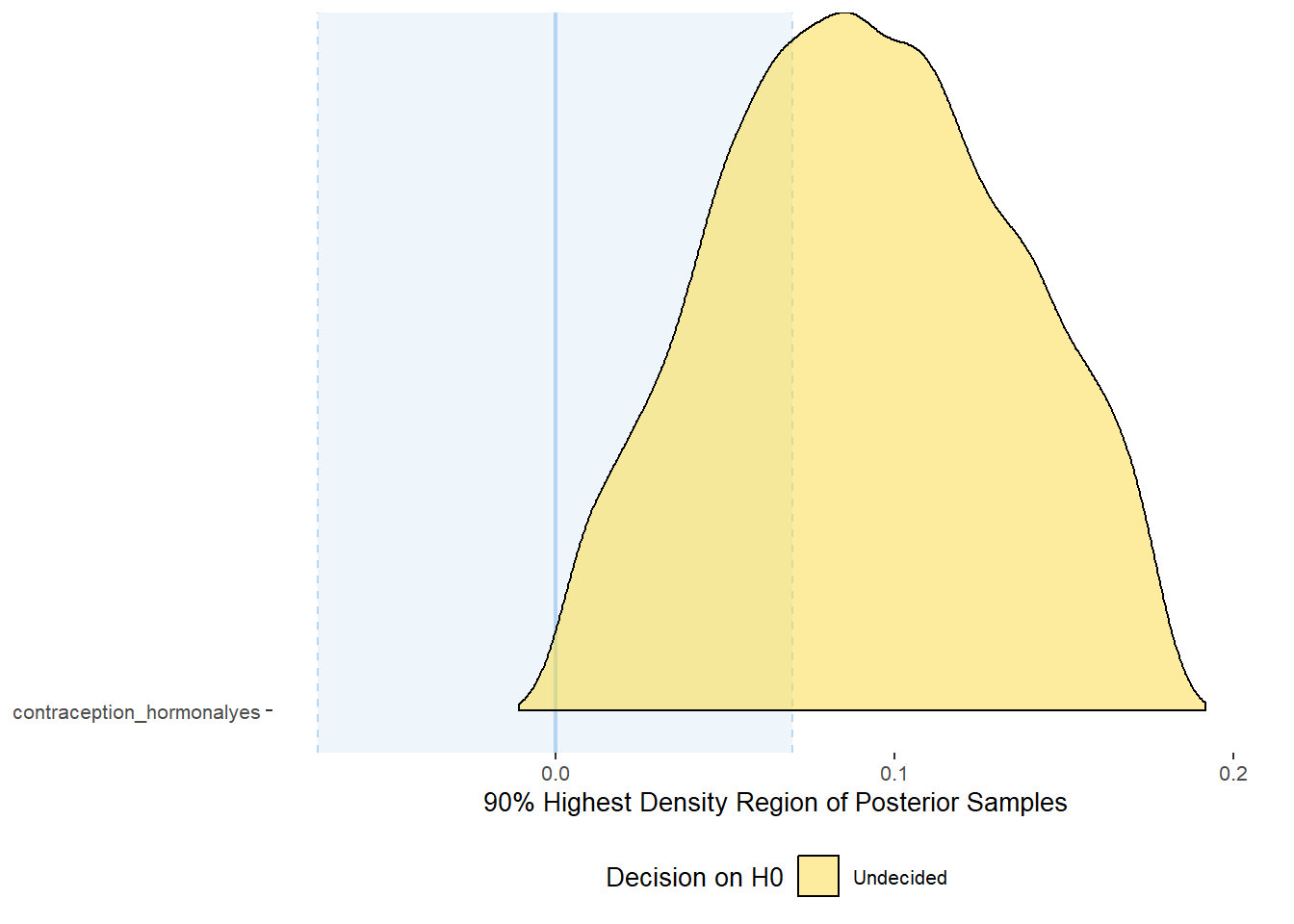
## # A tibble: 1 x 10
##   Parameter          CI ROPE_low ROPE_high ROPE_Percentage ROPE_Equivalence HDI_low HDI_high Effects Component
##   <chr>           <dbl>    <dbl>     <dbl>           <dbl> <chr>              <dbl>    <dbl> <chr>   <chr>
## 1 b_contraceptio~   0.9    -0.07      0.07           0.333 Undecided        0.00284    0.178 fixed   conditio~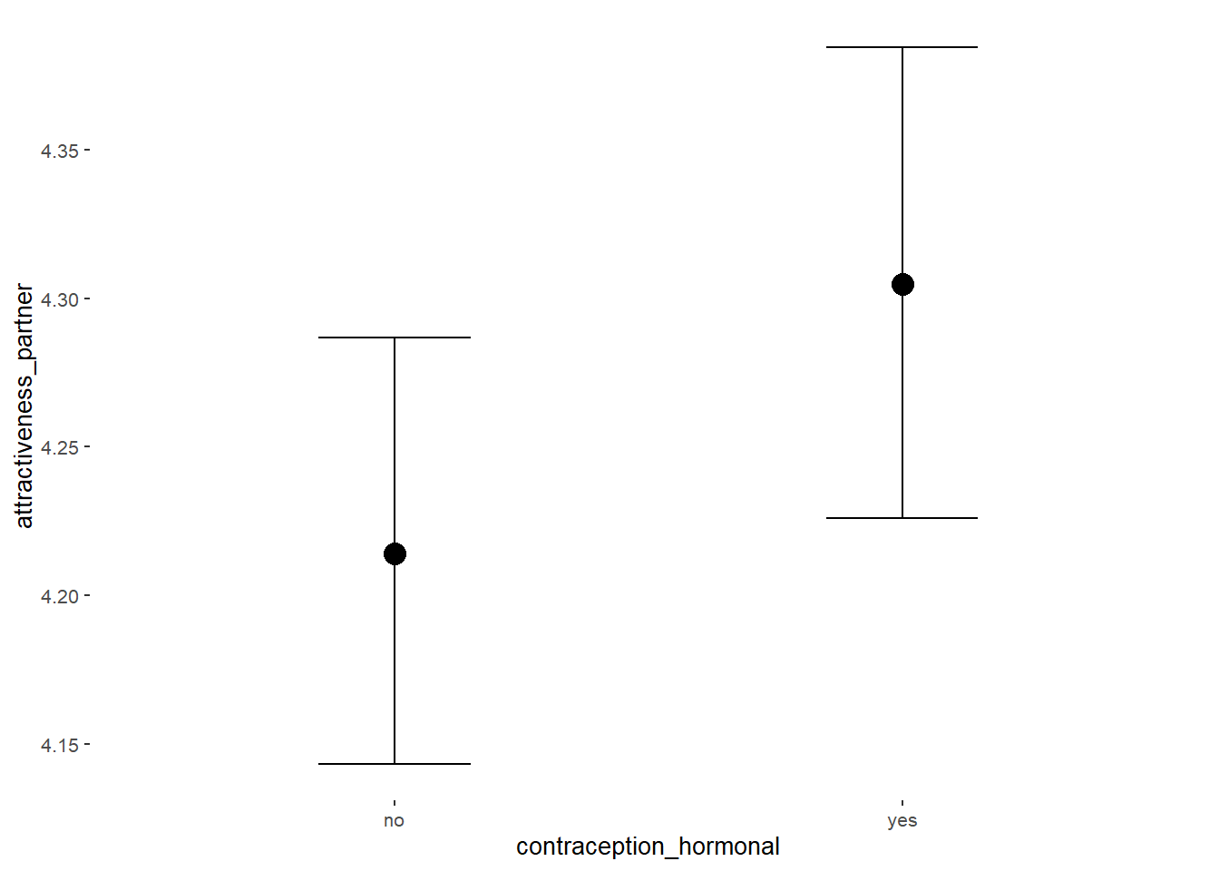
Forest Plot for Effect Sizes
m_hc_atrr %>%
  spread_draws(b_contraception_hormonalyes) %>%
  pivot_longer(cols = c(b_contraception_hormonalyes),
               names_to = "condition",
               values_to = "r_condition") %>%
  mutate(condition_mean = r_condition,
         group = ifelse(condition %contains% "b_contraception_hormonalyes",
                        "Contraception", NA),
         condition = ifelse(condition %contains% "b_contraception_hormonalyes",
                        "Hormonal Contraception", NA)) %>%
  ggplot(aes(y = condition,
             x = condition_mean,
             fill = stat(abs(x) < 0.07))) +
  stat_halfeye() +
  geom_vline(xintercept = c(-0.07, 0.07), linetype = "dotted") +
  apatheme +
  theme(legend.position = "none") +
  scale_fill_manual(values = c("gray80", "skyblue")) +
  labs(x = "Effect Size Estimates", y = "Predictors") +
  xlim (-0.6, 0.6)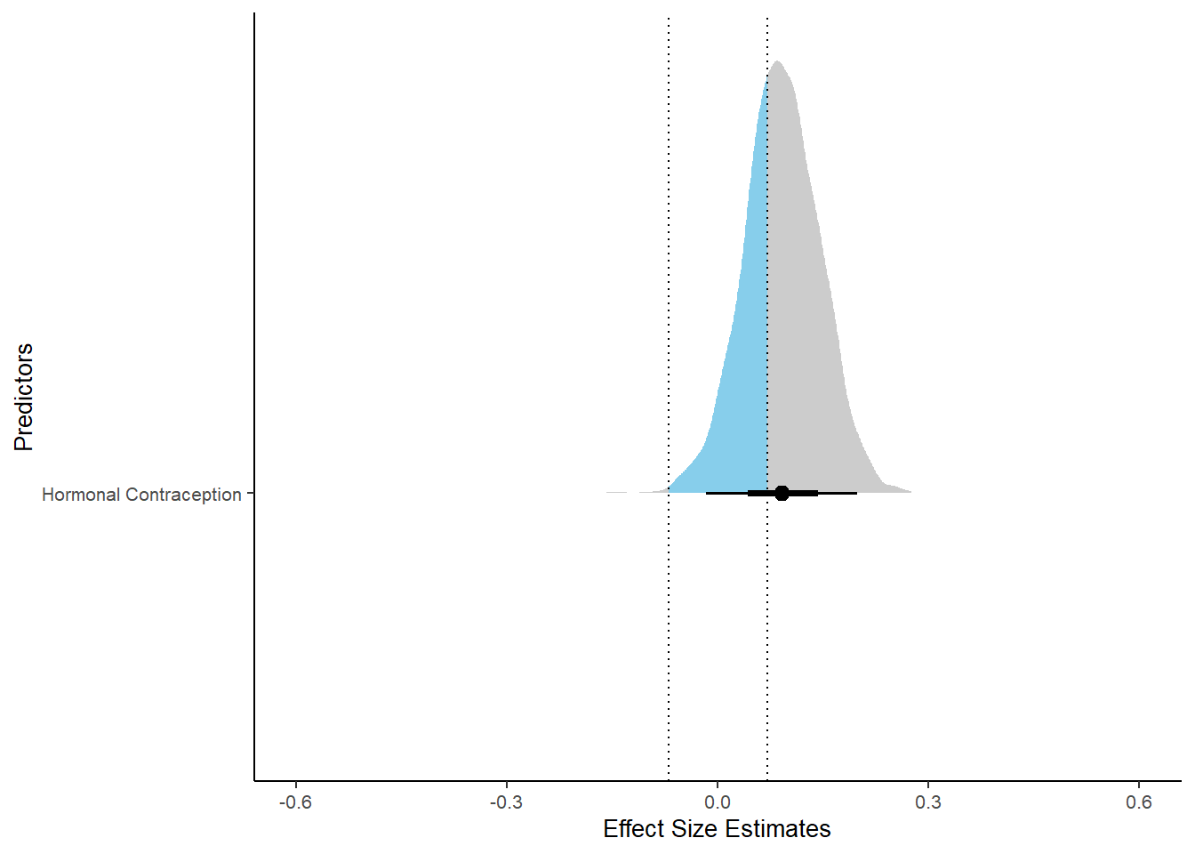
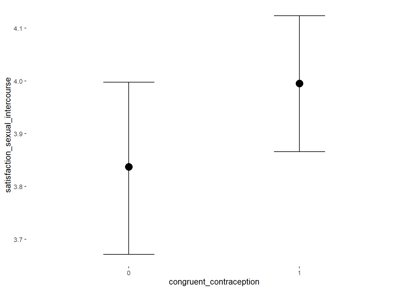
Relationship Satisfaction
Model
Summary
##  Family: gaussian
##   Links: mu = identity; sigma = identity
## Formula: relationship_satisfaction ~ contraception_hormonal
##    Data: data (Number of observations: 710)
##   Draws: 4 chains, each with iter = 2000; warmup = 1000; thin = 1;
##          total post-warmup draws = 4000
##
## Population-Level Effects:
##                           Estimate Est.Error l-90% CI u-90% CI Rhat Bulk_ESS Tail_ESS
## Intercept                     3.35      0.02     3.32     3.39 1.00     4081     2899
## contraception_hormonalyes     0.09      0.03     0.04     0.15 1.00     4051     2820
##
## Family Specific Parameters:
##       Estimate Est.Error l-90% CI u-90% CI Rhat Bulk_ESS Tail_ESS
## sigma     0.42      0.01     0.40     0.44 1.00     4667     2871
##
## Draws were sampled using sampling(NUTS). For each parameter, Bulk_ESS
## and Tail_ESS are effective sample size measures, and Rhat is the potential
## scale reduction factor on split chains (at convergence, Rhat = 1).
Comparison with ROPE
plot(equivalence_test(m_hc_relsat, range = c(-0.04, 0.04), ci = 0.90,
                      parameters = "contraception"))
## Picking joint bandwidth of 0.00443## Warning: Removed 399 rows containing non-finite values (stat_density_ridges).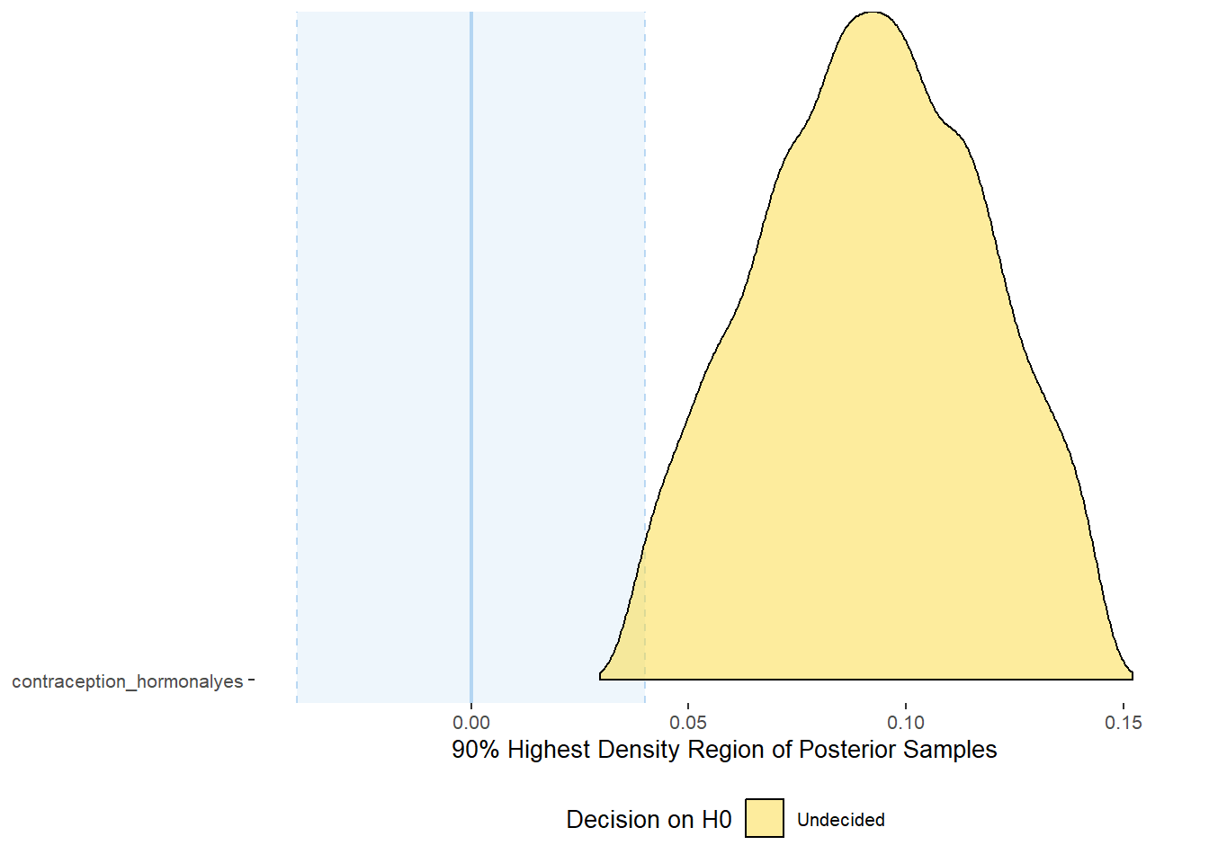
## # A tibble: 1 x 10
##   Parameter          CI ROPE_low ROPE_high ROPE_Percentage ROPE_Equivalence HDI_low HDI_high Effects Component
##   <chr>           <dbl>    <dbl>     <dbl>           <dbl> <chr>              <dbl>    <dbl> <chr>   <chr>
## 1 b_contraceptio~   0.9    -0.04      0.04          0.0119 Undecided         0.0377    0.144 fixed   conditio~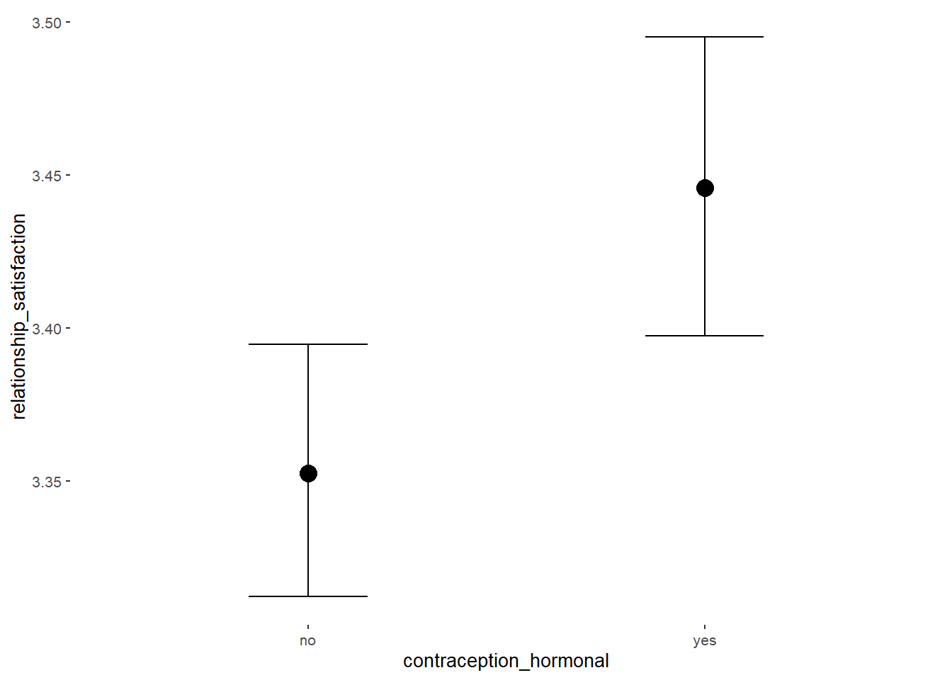
Forest Plot for Effect Sizes
m_hc_relsat %>%
  spread_draws(b_contraception_hormonalyes) %>%
  pivot_longer(cols = c(b_contraception_hormonalyes),
               names_to = "condition",
               values_to = "r_condition") %>%
  mutate(condition_mean = r_condition,
         group = ifelse(condition %contains% "b_contraception_hormonalyes",
                        "Contraception", NA),
         condition = ifelse(condition %contains% "b_contraception_hormonalyes",
                        "Hormonal Contraception", NA)) %>%
  ggplot(aes(y = condition,
             x = condition_mean,
             fill = stat(abs(x) < 0.04))) +
  stat_halfeye() +
  geom_vline(xintercept = c(-0.04, 0.04), linetype = "dotted") +
  apatheme +
  theme(legend.position = "none") +
  scale_fill_manual(values = c("gray80", "skyblue")) +
  labs(x = "Effect Size Estimates", y = "Predictors") +
  xlim (-0.6, 0.6)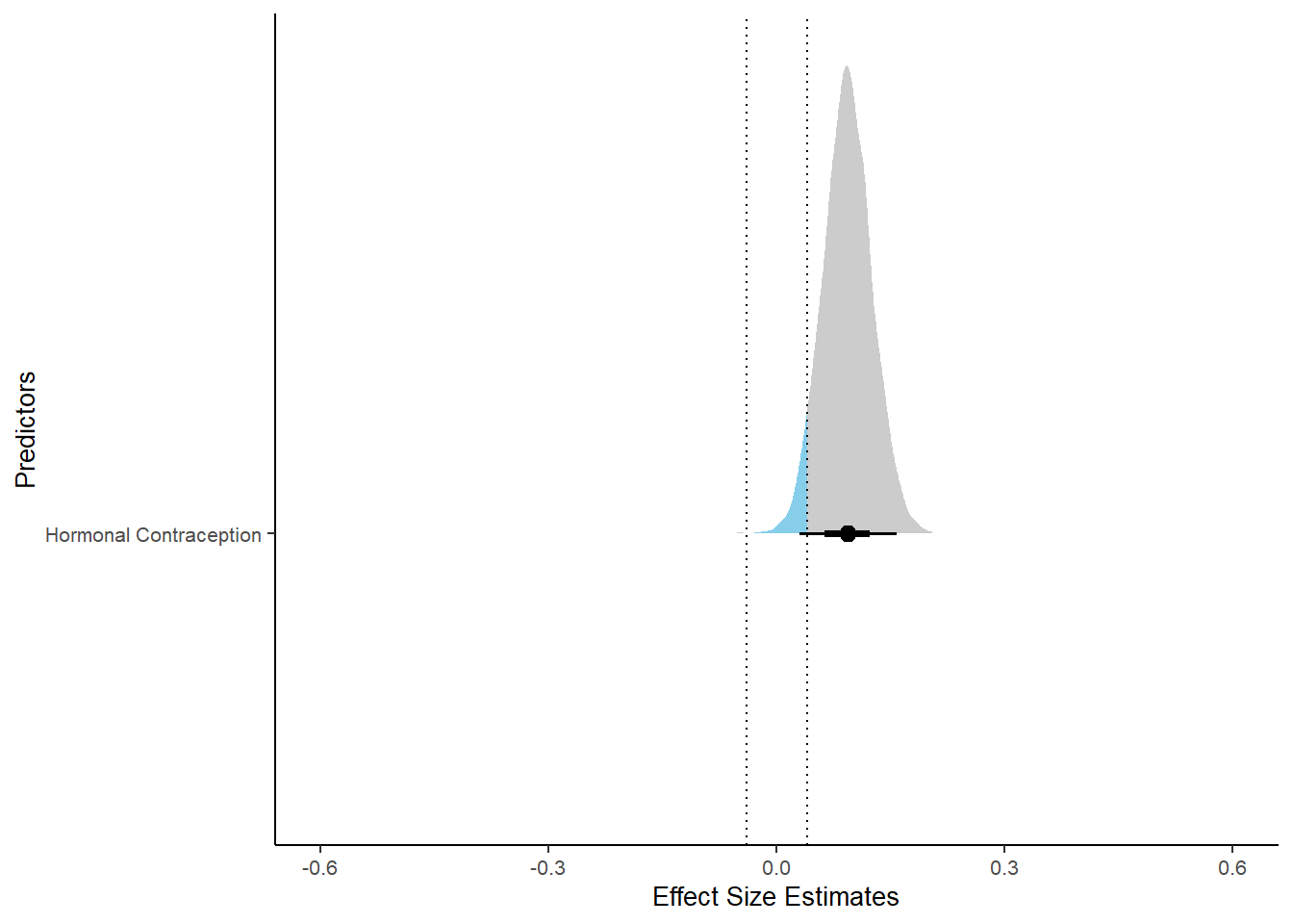
Sexual Satisfaction
Model
Summary
##  Family: gaussian
##   Links: mu = identity; sigma = identity
## Formula: satisfaction_sexual_intercourse ~ contraception_hormonal
##    Data: data (Number of observations: 710)
##   Draws: 4 chains, each with iter = 2000; warmup = 1000; thin = 1;
##          total post-warmup draws = 4000
##
## Population-Level Effects:
##                           Estimate Est.Error l-90% CI u-90% CI Rhat Bulk_ESS Tail_ESS
## Intercept                     3.93      0.05     3.85     4.02 1.00     4760     3121
## contraception_hormonalyes     0.19      0.08     0.06     0.32 1.00     4380     3040
##
## Family Specific Parameters:
##       Estimate Est.Error l-90% CI u-90% CI Rhat Bulk_ESS Tail_ESS
## sigma     1.04      0.03     0.99     1.09 1.00     4047     2956
##
## Draws were sampled using sampling(NUTS). For each parameter, Bulk_ESS
## and Tail_ESS are effective sample size measures, and Rhat is the potential
## scale reduction factor on split chains (at convergence, Rhat = 1).
Comparison with ROPE
plot(equivalence_test(m_hc_sexsat, range = c(-0.11, 0.11), ci = 0.90,
                      parameters = "contraception"))
## Picking joint bandwidth of 0.0109## Warning: Removed 399 rows containing non-finite values (stat_density_ridges).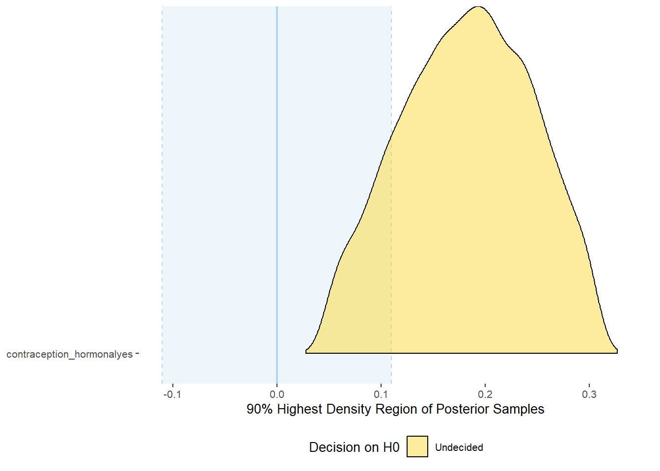
## # A tibble: 1 x 10
##   Parameter          CI ROPE_low ROPE_high ROPE_Percentage ROPE_Equivalence HDI_low HDI_high Effects Component
##   <chr>           <dbl>    <dbl>     <dbl>           <dbl> <chr>              <dbl>    <dbl> <chr>   <chr>
## 1 b_contraceptio~   0.9    -0.11      0.11           0.143 Undecided         0.0480    0.306 fixed   conditio~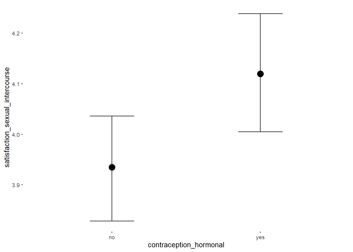
Forest Plot for Effect Sizes
m_hc_sexsat %>%
  spread_draws(b_contraception_hormonalyes) %>%
  pivot_longer(cols = c(b_contraception_hormonalyes),
               names_to = "condition",
               values_to = "r_condition") %>%
  mutate(condition_mean = r_condition,
         group = ifelse(condition %contains% "b_contraception_hormonalyes",
                        "Contraception", NA),
         condition = ifelse(condition %contains% "b_contraception_hormonalyes",
                        "Hormonal Contraception", NA)) %>%
  ggplot(aes(y = condition,
             x = condition_mean,
             fill = stat(abs(x) < 0.11))) +
  stat_halfeye() +
  geom_vline(xintercept = c(-0.11, 0.11), linetype = "dotted") +
  apatheme +
  theme(legend.position = "none") +
  scale_fill_manual(values = c("gray80", "skyblue")) +
  labs(x = "Effect Size Estimates", y = "Predictors") +
  xlim (-0.6, 0.6)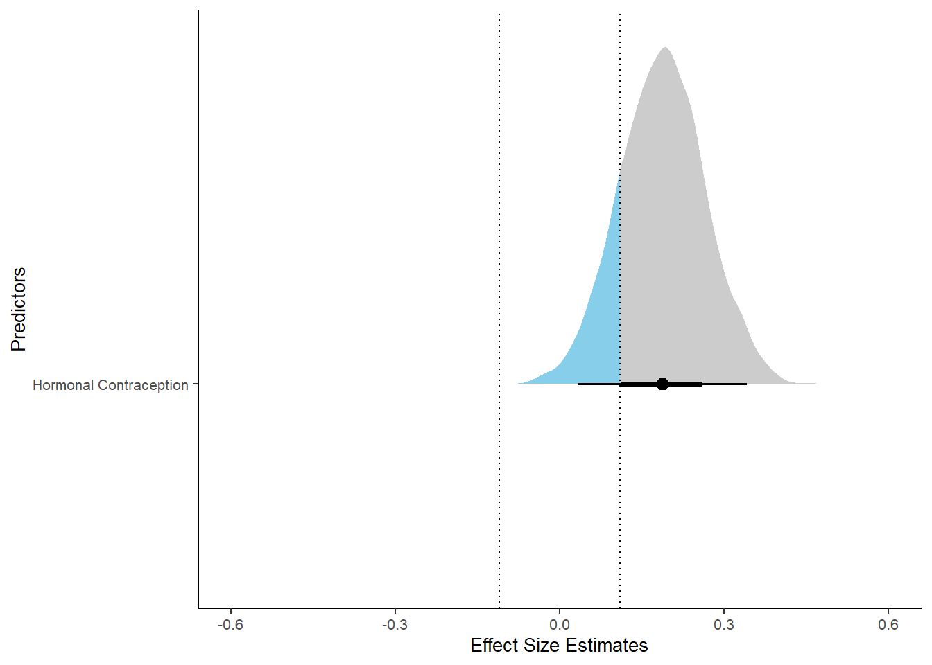
Libido
Model
Summary
##  Family: gaussian
##   Links: mu = identity; sigma = identity
## Formula: diary_libido_mean ~ contraception_hormonal
##    Data: data (Number of observations: 910)
##   Draws: 4 chains, each with iter = 2000; warmup = 1000; thin = 1;
##          total post-warmup draws = 4000
##
## Population-Level Effects:
##                           Estimate Est.Error l-90% CI u-90% CI Rhat Bulk_ESS Tail_ESS
## Intercept                     1.18      0.02     1.14     1.22 1.00     4384     3207
## contraception_hormonalyes    -0.01      0.04    -0.08     0.06 1.00     4191     2611
##
## Family Specific Parameters:
##       Estimate Est.Error l-90% CI u-90% CI Rhat Bulk_ESS Tail_ESS
## sigma     0.59      0.01     0.57     0.62 1.00     3977     3271
##
## Draws were sampled using sampling(NUTS). For each parameter, Bulk_ESS
## and Tail_ESS are effective sample size measures, and Rhat is the potential
## scale reduction factor on split chains (at convergence, Rhat = 1).
Comparison with ROPE
plot(equivalence_test(m_hc_libido, range = c(-0.06, 0.06), ci = 0.90,
                      parameters = "contraception"))
## Picking joint bandwidth of 0.00577## Warning: Removed 399 rows containing non-finite values (stat_density_ridges).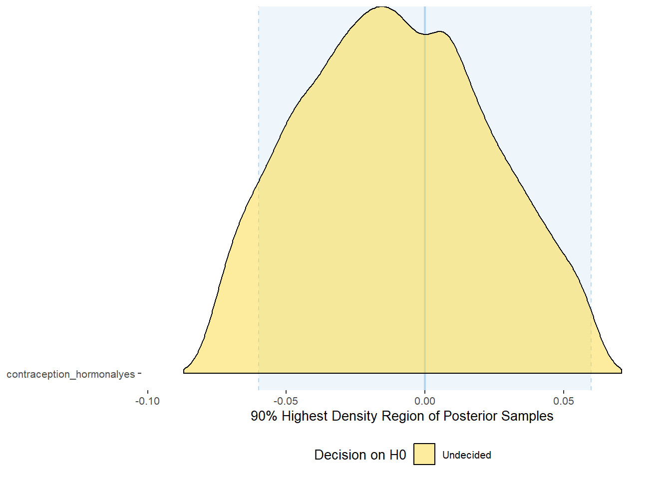
## # A tibble: 1 x 10
##   Parameter          CI ROPE_low ROPE_high ROPE_Percentage ROPE_Equivalence HDI_low HDI_high Effects Component
##   <chr>           <dbl>    <dbl>     <dbl>           <dbl> <chr>              <dbl>    <dbl> <chr>   <chr>
## 1 b_contraceptio~   0.9    -0.06      0.06           0.928 Undecided        -0.0765   0.0604 fixed   conditio~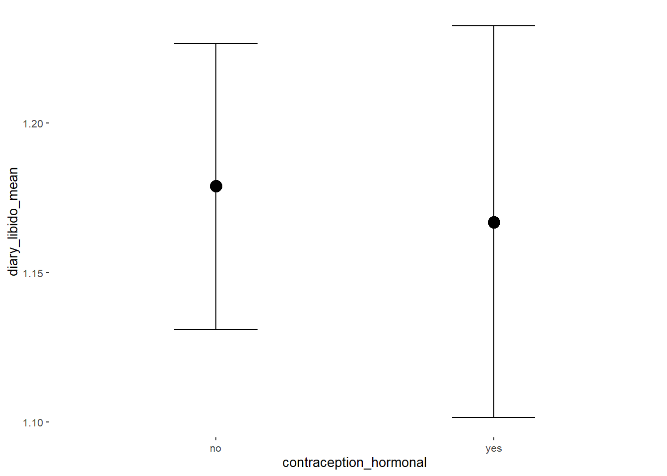
Forest Plot for Effect Sizes
m_hc_libido %>%
  spread_draws(b_contraception_hormonalyes) %>%
  pivot_longer(cols = c(b_contraception_hormonalyes),
               names_to = "condition",
               values_to = "r_condition") %>%
  mutate(condition_mean = r_condition,
         group = ifelse(condition %contains% "b_contraception_hormonalyes",
                        "Contraception", NA),
         condition = ifelse(condition %contains% "b_contraception_hormonalyes",
                        "Hormonal Contraception", NA)) %>%
  ggplot(aes(y = condition,
             x = condition_mean,
             fill = stat(abs(x) < 0.06))) +
  stat_halfeye() +
  geom_vline(xintercept = c(-0.06, 0.06), linetype = "dotted") +
  apatheme +
  theme(legend.position = "none") +
  scale_fill_manual(values = c("gray80", "skyblue")) +
  labs(x = "Effect Size Estimates", y = "Predictors") +
  xlim (-0.6, 0.6)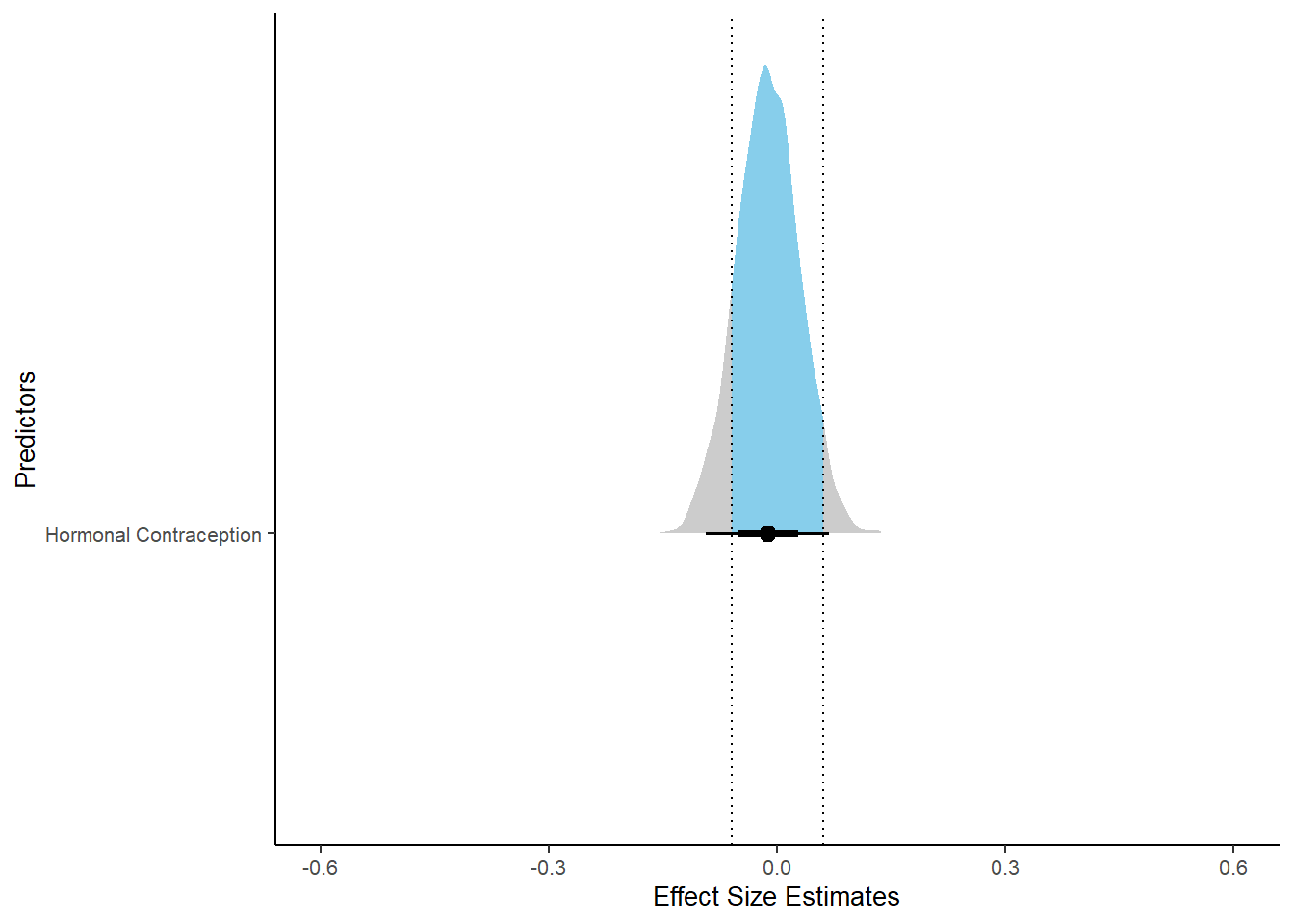
Sexual Frequency (Penetrative Intercourse)
Model
Summary
##  Family: poisson
##   Links: mu = log
## Formula: diary_sex_active_sex_sum ~ offset(log(number_of_days)) + contraception_hormonal
##    Data: data (Number of observations: 839)
##   Draws: 4 chains, each with iter = 2000; warmup = 1000; thin = 1;
##          total post-warmup draws = 4000
##
## Population-Level Effects:
##                           Estimate Est.Error l-90% CI u-90% CI Rhat Bulk_ESS Tail_ESS
## Intercept                    -2.09      0.02    -2.12    -2.06 1.00     3055     2548
## contraception_hormonalyes     0.20      0.03     0.16     0.25 1.00     3383     2771
##
## Draws were sampled using sampling(NUTS). For each parameter, Bulk_ESS
## and Tail_ESS are effective sample size measures, and Rhat is the potential
## scale reduction factor on split chains (at convergence, Rhat = 1).
Comparison with ROPE
plot(equivalence_test(m_hc_sexfreqpen, range = c(-0.05, 0.05)), ci = 0.90,
                      parameters = "contraception")
## Picking joint bandwidth of 0.00389## Warning: Removed 199 rows containing non-finite values (stat_density_ridges).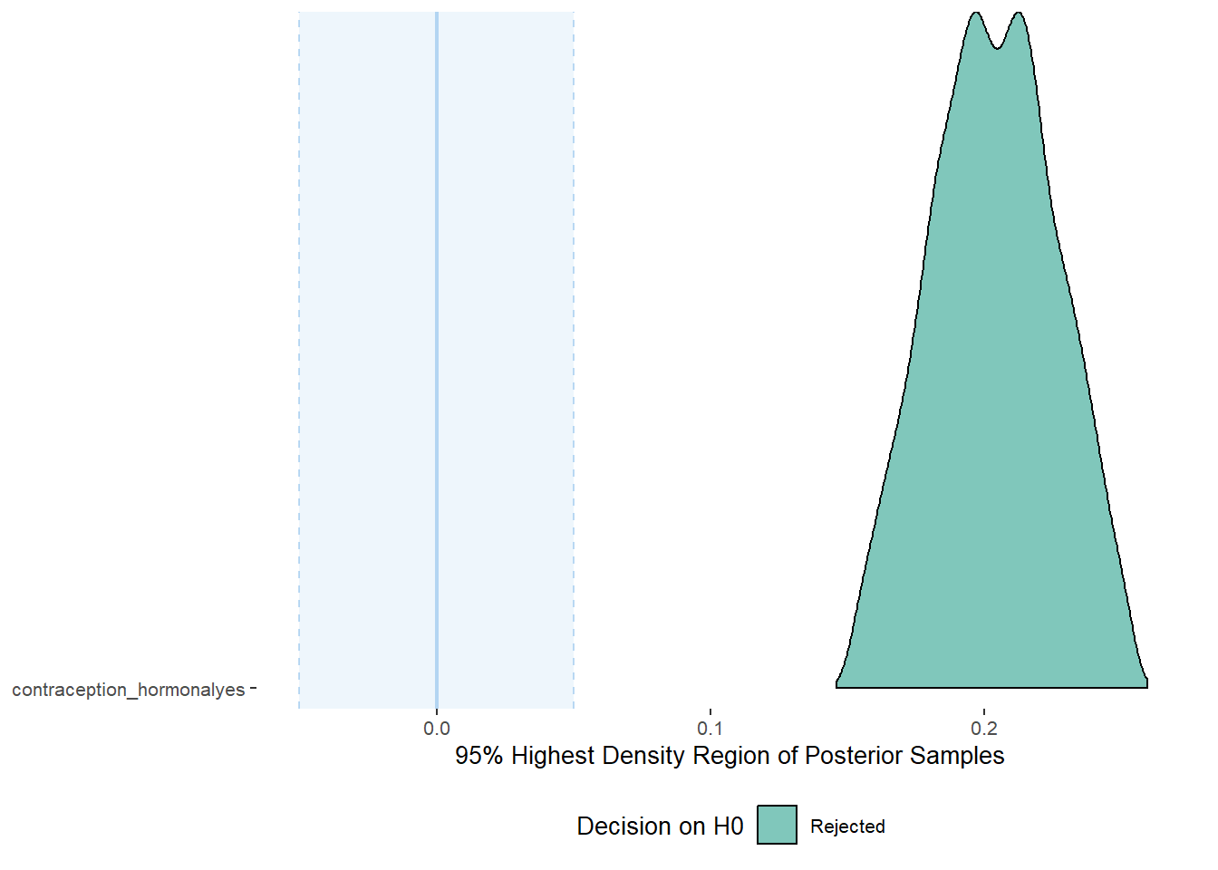
## # A tibble: 1 x 10
##   Parameter          CI ROPE_low ROPE_high ROPE_Percentage ROPE_Equivalence HDI_low HDI_high Effects Component
##   <chr>           <dbl>    <dbl>     <dbl>           <dbl> <chr>              <dbl>    <dbl> <chr>   <chr>
## 1 b_contraceptio~   0.9    -0.05      0.05               0 Rejected           0.161    0.245 fixed   conditio~
Plots
conditional_effects(m_hc_sexfreqpen,
                    effects = "contraception_hormonal",
                    conditions = data.frame(number_of_days = 1))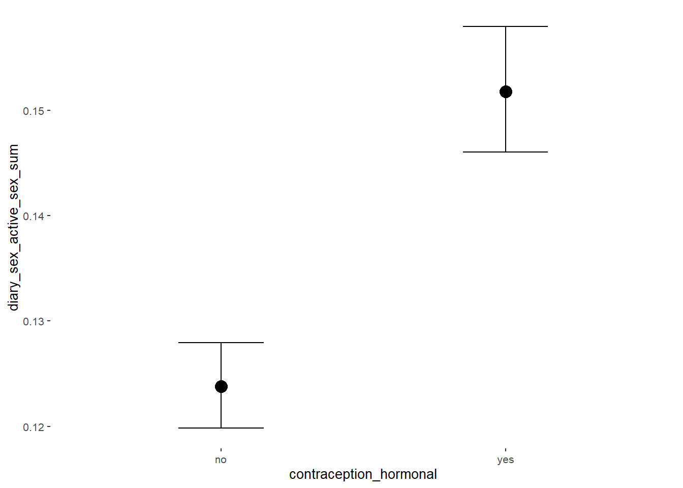
Forest Plot for Effect Sizes
m_hc_sexfreqpen %>%
  spread_draws(b_contraception_hormonalyes) %>%
  pivot_longer(cols = c(b_contraception_hormonalyes),
               names_to = "condition",
               values_to = "r_condition") %>%
  mutate(condition_mean = r_condition,
         group = ifelse(condition %contains% "b_contraception_hormonalyes",
                        "Contraception", NA),
         condition = ifelse(condition %contains% "b_contraception_hormonalyes",
                        "Hormonal Contraception", NA)) %>%
  ggplot(aes(y = condition,
             x = condition_mean,
             fill = stat(abs(x) < 0.05))) +
  stat_halfeye() +
  geom_vline(xintercept = c(-0.05, 0.05), linetype = "dotted") +
  apatheme +
  theme(legend.position = "none") +
  scale_fill_manual(values = c("gray80", "skyblue")) +
  labs(x = "Effect Size Estimates", y = "Predictors")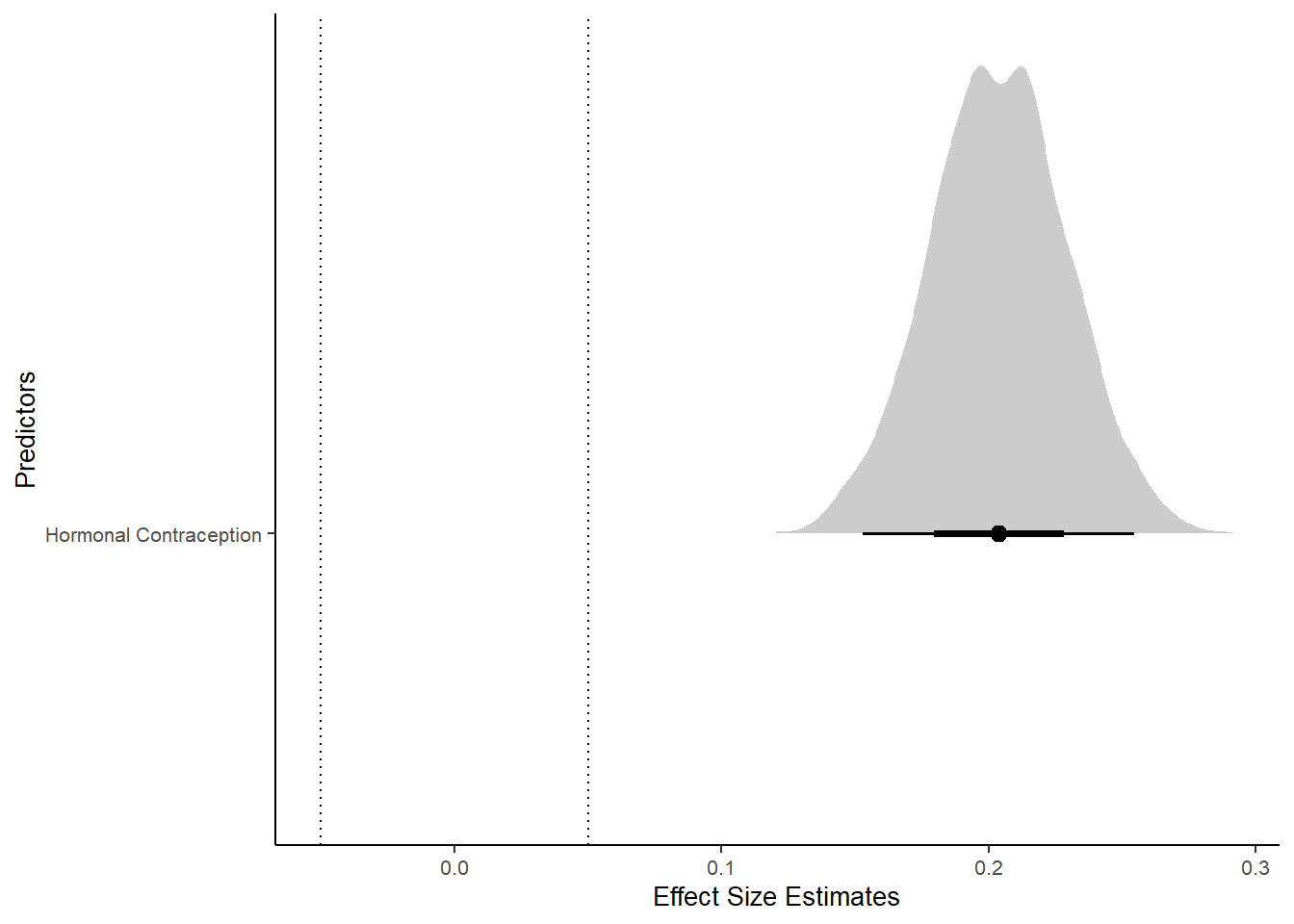
Masturbation Frequency
Model
Summary
##  Family: poisson
##   Links: mu = log
## Formula: diary_masturbation_sum ~ offset(log(number_of_days)) + contraception_hormonal
##    Data: data (Number of observations: 839)
##   Draws: 4 chains, each with iter = 2000; warmup = 1000; thin = 1;
##          total post-warmup draws = 4000
##
## Population-Level Effects:
##                           Estimate Est.Error l-90% CI u-90% CI Rhat Bulk_ESS Tail_ESS
## Intercept                    -1.88      0.02    -1.90    -1.85 1.00     3763     2771
## contraception_hormonalyes    -0.44      0.03    -0.49    -0.39 1.00     2664     2128
##
## Draws were sampled using sampling(NUTS). For each parameter, Bulk_ESS
## and Tail_ESS are effective sample size measures, and Rhat is the potential
## scale reduction factor on split chains (at convergence, Rhat = 1).
Comparison with ROPE
plot(equivalence_test(m_hc_masfreq, range = c(-0.05, 0.05), ci = 0.90,
                      parameters = "contraception"))
## Picking joint bandwidth of 0.00402## Warning: Removed 399 rows containing non-finite values (stat_density_ridges).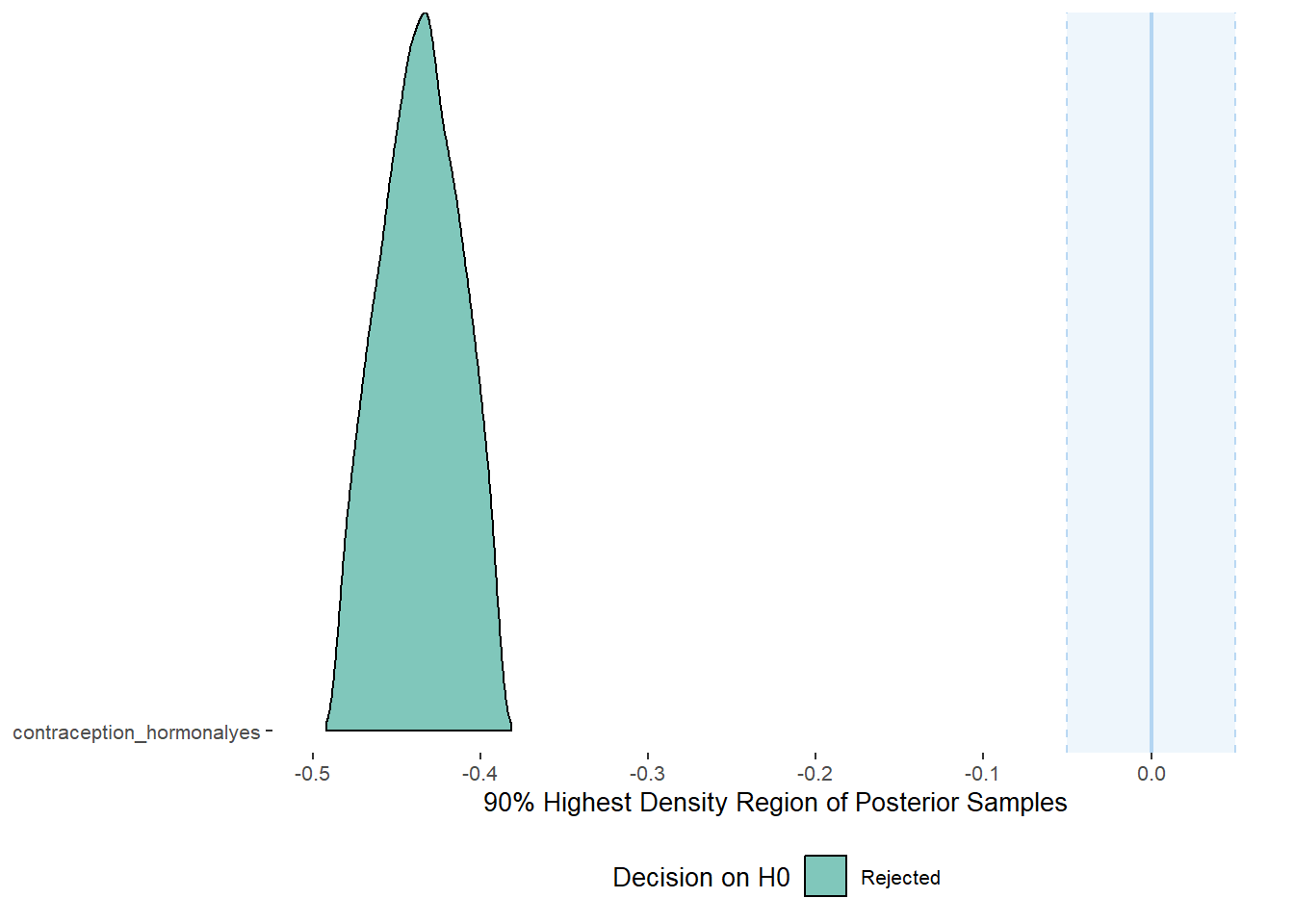
## # A tibble: 1 x 10
##   Parameter          CI ROPE_low ROPE_high ROPE_Percentage ROPE_Equivalence HDI_low HDI_high Effects Component
##   <chr>           <dbl>    <dbl>     <dbl>           <dbl> <chr>              <dbl>    <dbl> <chr>   <chr>
## 1 b_contraceptio~   0.9    -0.05      0.05               0 Rejected          -0.485   -0.389 fixed   conditio~
Plots
conditional_effects(m_hc_masfreq,
                    effects = "contraception_hormonal",
                    conditions = data.frame(number_of_days = 1))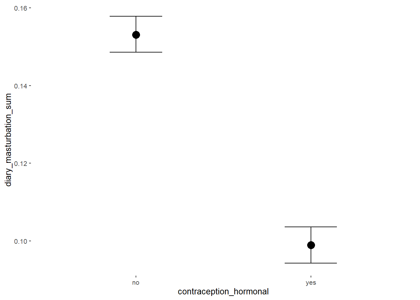
Forest Plot for Effect Sizes
m_hc_masfreq %>%
  spread_draws(b_contraception_hormonalyes) %>%
  pivot_longer(cols = c(b_contraception_hormonalyes),
               names_to = "condition",
               values_to = "r_condition") %>%
  mutate(condition_mean = r_condition,
         group = ifelse(condition %contains% "b_contraception_hormonalyes",
                        "Contraception", NA),
         condition = ifelse(condition %contains% "b_contraception_hormonalyes",
                        "Hormonal Contraception", NA)) %>%
  ggplot(aes(y = condition,
             x = condition_mean,
             fill = stat(abs(x) < 0.05))) +
  stat_halfeye() +
  geom_vline(xintercept = c(-0.05, 0.05), linetype = "dotted") +
  apatheme +
  theme(legend.position = "none") +
  scale_fill_manual(values = c("gray80", "skyblue")) +
  labs(x = "Effect Size Estimates", y = "Predictors")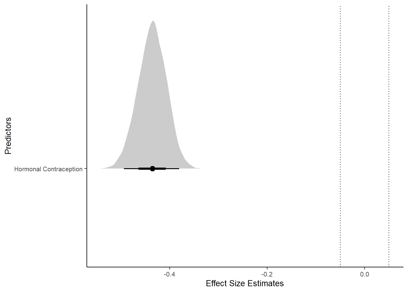
Controlled Models: Effects of Hormonal Contraceptives
Attractiveness of Partner
Model
Summary
## Warning: Parts of the model have not converged (some Rhats are > 1.05). Be careful when analysing the results!
## We recommend running more iterations and/or setting stronger priors.
## Family: gaussian
## Links: mu = identity; sigma = identity
## Formula: attractiveness_partner ~ contraception_hormonal + age + net_income + relationship_duration_factor + education_years + bfi_extra + bfi_neuro + bfi_agree + bfi_consc + bfi_open + religiosity
## Data: data (Number of observations: 710)
## Draws: 4 chains, each with iter = 2000; warmup = 1000; thin = 1;
## total post-warmup draws = 4000
##
## Population-Level Effects:
## Estimate Est.Error l-90% CI u-90% CI Rhat Bulk_ESS
## Intercept 66.77 410.67 -573.74 702.13 2.75 5
## contraception_hormonalyes 0.10 0.06 0.01 0.21 1.03 52
## age 0.00 0.01 -0.01 0.01 1.05 66
## net_incomeeuro_500_1000 0.01 0.07 -0.11 0.13 1.04 65
## net_incomeeuro_1000_2000 0.10 0.08 -0.02 0.23 1.04 76
## net_incomeeuro_2000_3000 0.10 0.11 -0.10 0.27 1.05 65
## net_incomeeuro_gt_3000 0.04 0.19 -0.29 0.37 1.16 22
## net_incomedont_tell 0.06 0.18 -0.24 0.37 1.14 32
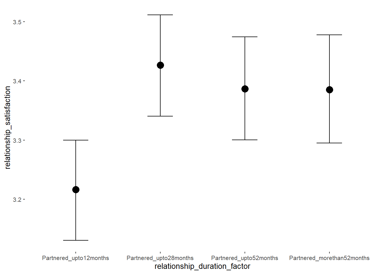
## relationship_duration_factorPartnered_upto12months -63.34 410.63 -699.05 576.66 2.75 5
## relationship_duration_factorPartnered_upto28months -63.24 410.63 -698.98 576.79 2.75 5
## relationship_duration_factorPartnered_upto52months -63.41 410.63 -699.14 576.62 2.75 5
## relationship_duration_factorPartnered_morethan52months -63.46 410.63 -699.18 576.49 2.75 5
## education_years 0.00 0.01 -0.01 0.01 1.09 40
## bfi_extra 0.04 0.04 -0.02 0.10 1.17 19
## bfi_neuro 0.01 0.04 -0.06 0.08 1.38 9
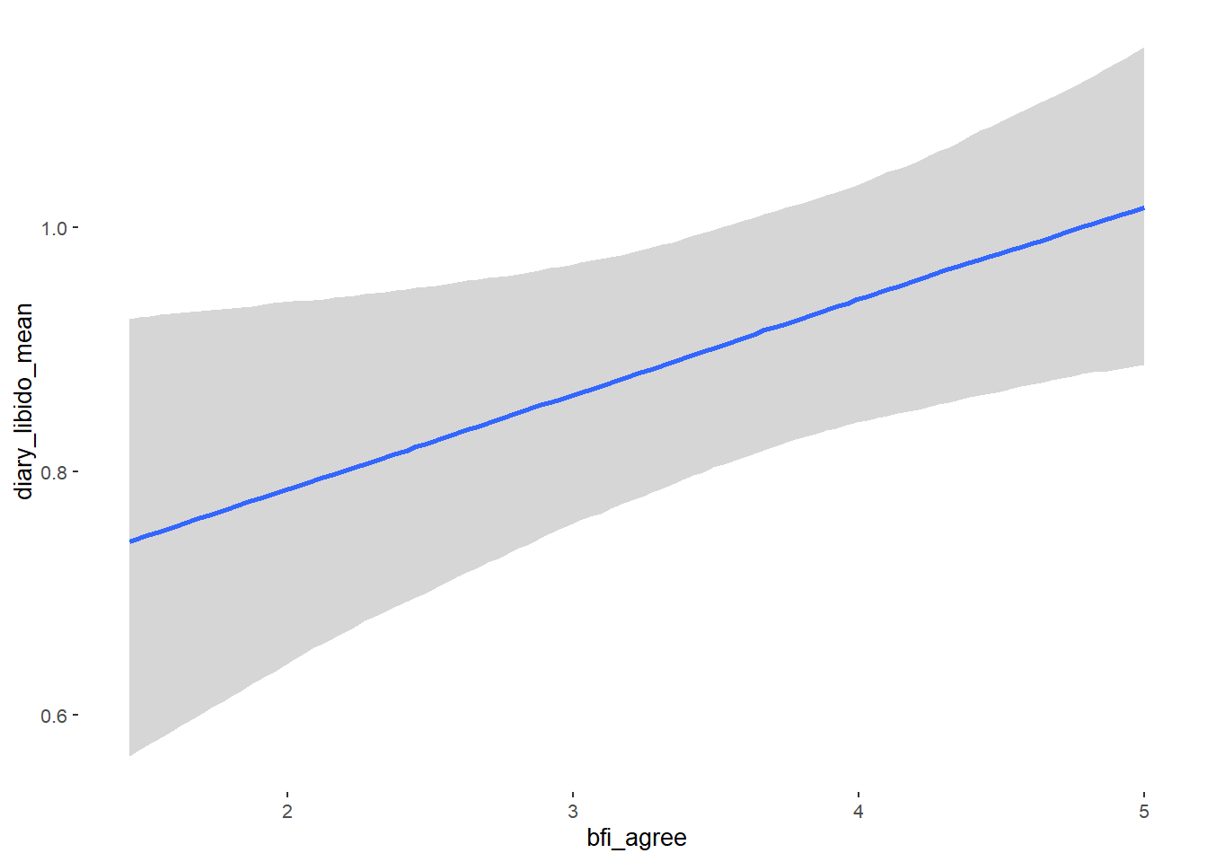
## bfi_agree 0.09 0.05 0.01 0.18 1.23 15
## bfi_consc 0.02 0.04 -0.04 0.08 1.09 61
## bfi_open 0.02 0.04 -0.05 0.09 1.06 64
## religiosity 0.01 0.02 -0.03 0.04 1.06 76
## Tail_ESS
## Intercept NA
## contraception_hormonalyes NA
## age NA
## net_incomeeuro_500_1000 NA
## net_incomeeuro_1000_2000 NA
## net_incomeeuro_2000_3000 NA
## net_incomeeuro_gt_3000 NA
## net_incomedont_tell NA
## relationship_duration_factorPartnered_upto12months NA
## relationship_duration_factorPartnered_upto28months NA
## relationship_duration_factorPartnered_upto52months NA
## relationship_duration_factorPartnered_morethan52months NA
## education_years NA
## bfi_extra NA
## bfi_neuro NA
## bfi_agree NA
## bfi_consc NA
## bfi_open NA
## religiosity NA
##
## Family Specific Parameters:
## Estimate Est.Error l-90% CI u-90% CI Rhat Bulk_ESS Tail_ESS
## sigma 0.73 0.02 0.70 0.76 1.11 30 NA
##
## Draws were sampled using sampling(NUTS). For each parameter, Bulk_ESS
## and Tail_ESS are effective sample size measures, and Rhat is the potential
## scale reduction factor on split chains (at convergence, Rhat = 1).Comparison with ROPE
plot(equivalence_test(m_hc_atrr_controlled, range = c(-0.07, 0.07), ci = 0.90,
                      parameters = "contraception"))
## Picking joint bandwidth of 0.00787## Warning: Removed 399 rows containing non-finite values (stat_density_ridges).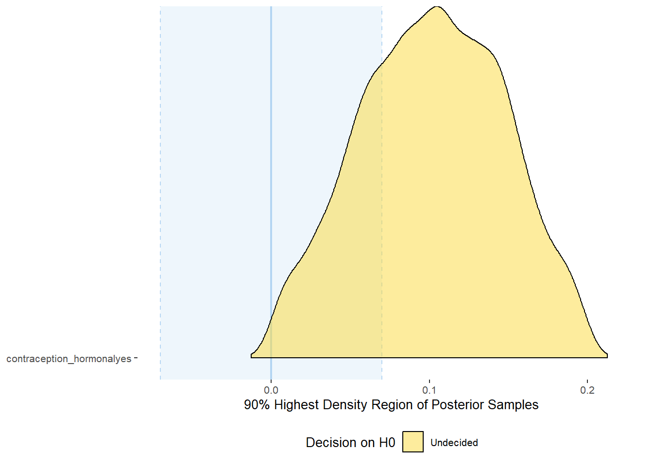
equivalence_test(m_hc_atrr_controlled, range = c(-0.07, 0.07), ci = 0.90,
                      parameters = "contraception")
## # A tibble: 1 x 10
## Parameter CI ROPE_low ROPE_high ROPE_Percentage ROPE_Equivalence HDI_low HDI_high Effects Component
## <chr> <dbl> <dbl> <dbl> <dbl> <chr> <dbl> <dbl> <chr> <chr>
## 1 b_contraceptio~ 0.9 -0.07 0.07 0.264 Undecided 0.00146 0.199 fixed conditio~
Forest Plot for Effect Sizes
m_hc_atrr_controlled %>%
  spread_draws(b_contraception_hormonalyes,
               b_age,
               b_net_incomeeuro_500_1000, b_net_incomeeuro_1000_2000,
               b_net_incomeeuro_2000_3000, b_net_incomeeuro_gt_3000, b_net_incomedont_tell,
               b_relationship_duration_factorPartnered_upto28months,
               b_relationship_duration_factorPartnered_upto52months,
               b_relationship_duration_factorPartnered_morethan52months,
               b_education_years,
               b_bfi_extra, b_bfi_neuro, b_bfi_agree, b_bfi_consc, b_bfi_open,
               b_religiosity) %>%
  pivot_longer(cols = c(b_contraception_hormonalyes,
                        b_age,
               b_net_incomeeuro_500_1000, b_net_incomeeuro_1000_2000,
               b_net_incomeeuro_2000_3000, b_net_incomeeuro_gt_3000, b_net_incomedont_tell,
               b_relationship_duration_factorPartnered_upto28months,
               b_relationship_duration_factorPartnered_upto52months,
               b_relationship_duration_factorPartnered_morethan52months,
               b_education_years,
               b_bfi_extra, b_bfi_neuro, b_bfi_agree, b_bfi_consc, b_bfi_open,
               b_religiosity),
               names_to = "condition",
               values_to = "r_condition") %>%
  mutate(condition_mean = r_condition,
         group = ifelse(condition %contains% "b_relationship_duration_factor",
                        "Relationship Duration",
                        ifelse(condition %contains% "b_net_income",
                               "Income",
                               NA)),
         group = ifelse(condition %contains% "b_contraception_hormonalyes",
                        "Contraception", group),
         condition = ifelse(condition %contains% "b_contraception_hormonalyes",
                        "Hormonal Contraception", condition),
         condition = ifelse(condition == "b_age", "Age",
                ifelse(condition == "b_net_incomeeuro_500_1000", "500-1000 Euro",
                ifelse(condition == "b_net_incomeeuro_1000_2000", "1000-2000 Euro",
                ifelse(condition == "b_net_incomeeuro_2000_3000", "2000-3000 Euro",
                ifelse(condition == "b_net_incomeeuro_gt_3000", ">3000 Euro",
                ifelse(condition == "b_net_incomedont_tell", "do not tell",
                ifelse(condition == "b_relationship_duration_factorPartnered_upto28months",
                       "13-28 months",
                ifelse(condition == "b_relationship_duration_factorPartnered_upto52months",
                       "29-52 months",
                ifelse(condition == "b_relationship_duration_factorPartnered_morethan52months",
                       ">52 months",
                ifelse(condition == "b_education_years", "Years of Education",
                ifelse(condition == "b_bfi_extra", "Extraversion",
                ifelse(condition == "b_bfi_neuro", "Neuroticism",
                ifelse(condition == "b_bfi_agree", "Agreeableness",
                ifelse(condition == "b_bfi_consc", "Conscientiousness",
                ifelse(condition == "b_bfi_open", "Openness",
                ifelse(condition == "b_religiosity", "Religiosity",
                       condition)))))))))))))))),
         group = ifelse(is.na(group), condition, group),
         condition = factor(condition, levels = rev(c("Hormonal Contraception", "Age",
                                        "500-1000 Euro", "1000-2000 Euro",
                                        "2000-3000 Euro", ">3000 Euro", "do not tell",
                                        "13-28 months", "29-52 months",
                                        ">52 months",
                                        "Years of Education",
                                        "Extraversion", "Neuroticism", "Agreeableness",
                                         "Conscientiousness","Openness","Religiosity"))),
         group = factor(group, levels = c("Contraception", "Age", "Income",
                                          "Relationship Duration","Years of Education",
                                          "Extraversion", "Neuroticism", "Agreeableness",
                                         "Conscientiousness","Openness","Religiosity"))) %>%
  ggplot(aes(y = condition,
             x = condition_mean,
             fill = stat(abs(x) < 0.07))) +
  stat_halfeye() +
  geom_vline(xintercept = c(-0.07, 0.07), linetype = "dotted") +
  apatheme +
  theme(legend.position = "none") +
  scale_fill_manual(values = c("gray80", "skyblue")) +
  labs(x = "Effect Size Estimates", y = "Predictors")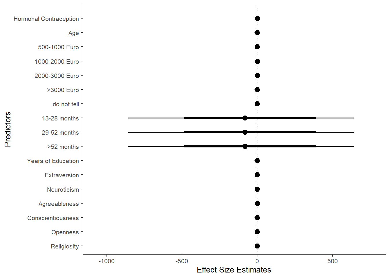
Relationship Satisfaction
Model
Summary
## Warning: Parts of the model have not converged (some Rhats are > 1.05). Be careful when analysing the results!
## We recommend running more iterations and/or setting stronger priors.
## Family: gaussian
## Links: mu = identity; sigma = identity
## Formula: relationship_satisfaction ~ contraception_hormonal + age + net_income + relationship_duration_factor + education_years + bfi_extra + bfi_neuro + bfi_agree + bfi_consc + bfi_open + religiosity
## Data: data (Number of observations: 710)
## Draws: 4 chains, each with iter = 2000; warmup = 1000; thin = 1;
## total post-warmup draws = 4000
##
## Population-Level Effects:
## Estimate Est.Error l-90% CI u-90% CI Rhat Bulk_ESS
## Intercept -99.95 348.02 -703.79 347.52 3.31 4
## contraception_hormonalyes 0.07 0.03 0.01 0.12 1.10 39
## age -0.00 0.00 -0.01 0.00 1.20 16
## net_incomeeuro_500_1000 0.04 0.04 -0.02 0.10 1.06 43
## net_incomeeuro_1000_2000 -0.02 0.05 -0.12 0.07 1.19 15
## net_incomeeuro_2000_3000 -0.00 0.08 -0.13 0.12 1.15 19
## net_incomeeuro_gt_3000 0.06 0.13 -0.17 0.26 1.12 26
## net_incomedont_tell -0.09 0.10 -0.26 0.07 1.21 16
## relationship_duration_factorPartnered_upto12months 103.24 348.03 -344.11 707.08 3.31 4
## relationship_duration_factorPartnered_upto28months 103.45 348.03 -343.88 707.37 3.31 4
## relationship_duration_factorPartnered_upto52months 103.41 348.03 -343.93 707.32 3.31 4
## relationship_duration_factorPartnered_morethan52months 103.40 348.04 -343.96 707.31 3.31 4
## education_years -0.00 0.00 -0.01 0.00 1.05 84
## bfi_extra 0.02 0.02 -0.01 0.06 1.10 30
## bfi_neuro 0.03 0.02 -0.01 0.07 1.04 51
## bfi_agree -0.03 0.03 -0.08 0.03 1.13 21
## bfi_consc 0.01 0.02 -0.04 0.04 1.16 20
## bfi_open -0.02 0.02 -0.05 0.02 1.08 69
## religiosity 0.03 0.01 0.01 0.05 1.06 41
## Tail_ESS
## Intercept NA
## contraception_hormonalyes NA
## age NA
## net_incomeeuro_500_1000 NA
## net_incomeeuro_1000_2000 NA
## net_incomeeuro_2000_3000 NA
## net_incomeeuro_gt_3000 NA
## net_incomedont_tell NA
## relationship_duration_factorPartnered_upto12months NA
## relationship_duration_factorPartnered_upto28months NA
## relationship_duration_factorPartnered_upto52months NA
## relationship_duration_factorPartnered_morethan52months NA
## education_years NA
## bfi_extra NA
## bfi_neuro NA
## bfi_agree NA
## bfi_consc NA
## bfi_open NA
## religiosity NA
##
## Family Specific Parameters:
## Estimate Est.Error l-90% CI u-90% CI Rhat Bulk_ESS Tail_ESS
## sigma 0.42 0.01 0.40 0.44 1.31 11 NA
##
## Draws were sampled using sampling(NUTS). For each parameter, Bulk_ESS
## and Tail_ESS are effective sample size measures, and Rhat is the potential
## scale reduction factor on split chains (at convergence, Rhat = 1).Comparison with ROPE
plot(equivalence_test(m_hc_relsat_controlled, range = c(-0.04, 0.04), ci = 0.90,
                      parameters = "contraception"))
## Picking joint bandwidth of 0.0044## Warning: Removed 399 rows containing non-finite values (stat_density_ridges).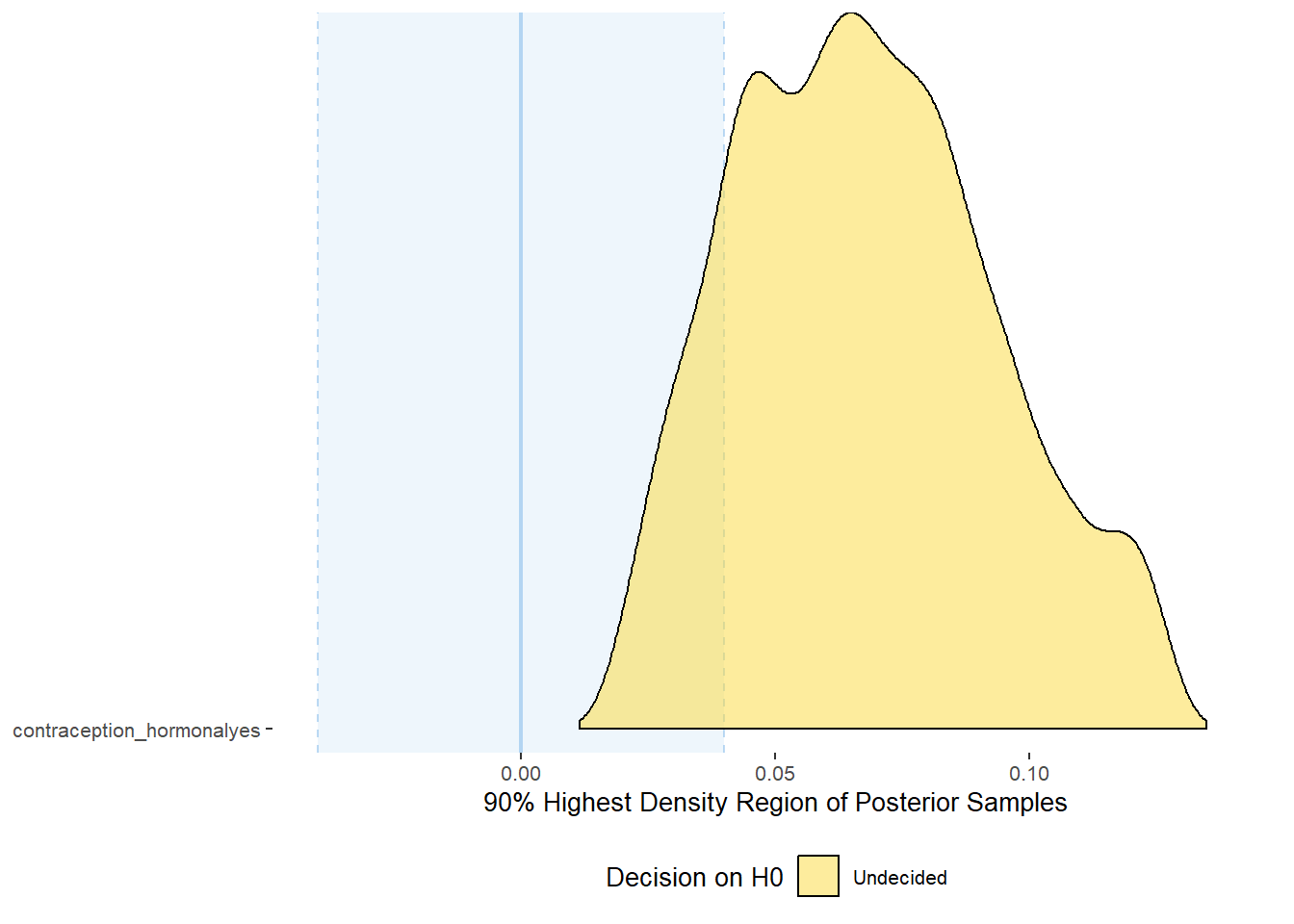
equivalence_test(m_hc_relsat_controlled, range = c(-0.04, 0.04), ci = 0.90,
                      parameters = "contraception")
## # A tibble: 1 x 10
## Parameter CI ROPE_low ROPE_high ROPE_Percentage ROPE_Equivalence HDI_low HDI_high Effects Component
## <chr> <dbl> <dbl> <dbl> <dbl> <chr> <dbl> <dbl> <chr> <chr>
## 1 b_contraceptio~ 0.9 -0.04 0.04 0.138 Undecided 0.0189 0.127 fixed conditio~


Forest Plot for Effect Sizes
m_hc_relsat_controlled %>%
  spread_draws(b_contraception_hormonalyes,
               b_age,
               b_net_incomeeuro_500_1000, b_net_incomeeuro_1000_2000,
               b_net_incomeeuro_2000_3000, b_net_incomeeuro_gt_3000, b_net_incomedont_tell,
               b_relationship_duration_factorPartnered_upto28months,
               b_relationship_duration_factorPartnered_upto52months,
               b_relationship_duration_factorPartnered_morethan52months,
               b_education_years,
               b_bfi_extra, b_bfi_neuro, b_bfi_agree, b_bfi_consc, b_bfi_open,
               b_religiosity) %>%
  pivot_longer(cols = c(b_contraception_hormonalyes,
                        b_age,
               b_net_incomeeuro_500_1000, b_net_incomeeuro_1000_2000,
               b_net_incomeeuro_2000_3000, b_net_incomeeuro_gt_3000, b_net_incomedont_tell,
               b_relationship_duration_factorPartnered_upto28months,
               b_relationship_duration_factorPartnered_upto52months,
               b_relationship_duration_factorPartnered_morethan52months,
               b_education_years,
               b_bfi_extra, b_bfi_neuro, b_bfi_agree, b_bfi_consc, b_bfi_open,
               b_religiosity),
               names_to = "condition",
               values_to = "r_condition") %>%
  mutate(condition_mean = r_condition,
         group = ifelse(condition %contains% "b_relationship_duration_factor",
                        "Relationship Duration",
                        ifelse(condition %contains% "b_net_income",
                               "Income",
                               NA)),
         group = ifelse(condition %contains% "b_contraception_hormonalyes",
                        "Contraception", group),
         condition = ifelse(condition %contains% "b_contraception_hormonalyes",
                        "Hormonal Contraception", condition),
         condition = ifelse(condition == "b_age", "Age",
                ifelse(condition == "b_net_incomeeuro_500_1000", "500-1000 Euro",
                ifelse(condition == "b_net_incomeeuro_1000_2000", "1000-2000 Euro",
                ifelse(condition == "b_net_incomeeuro_2000_3000", "2000-3000 Euro",
                ifelse(condition == "b_net_incomeeuro_gt_3000", ">3000 Euro",
                ifelse(condition == "b_net_incomedont_tell", "do not tell",
                ifelse(condition == "b_relationship_duration_factorPartnered_upto28months",
                       "13-28 months",
                ifelse(condition == "b_relationship_duration_factorPartnered_upto52months",
                       "29-52 months",
                ifelse(condition == "b_relationship_duration_factorPartnered_morethan52months",
                       ">52 months",
                ifelse(condition == "b_education_years", "Years of Education",
                ifelse(condition == "b_bfi_extra", "Extraversion",
                ifelse(condition == "b_bfi_neuro", "Neuroticism",
                ifelse(condition == "b_bfi_agree", "Agreeableness",
                ifelse(condition == "b_bfi_consc", "Conscientiousness",
                ifelse(condition == "b_bfi_open", "Openness",
                ifelse(condition == "b_religiosity", "Religiosity",
                       condition)))))))))))))))),
         group = ifelse(is.na(group), condition, group),
         condition = factor(condition, levels = rev(c("Hormonal Contraception", "Age",
                                        "500-1000 Euro", "1000-2000 Euro",
                                        "2000-3000 Euro", ">3000 Euro", "do not tell",
                                        "13-28 months", "29-52 months",
                                        ">52 months",
                                        "Years of Education",
                                        "Extraversion", "Neuroticism", "Agreeableness",
                                         "Conscientiousness","Openness","Religiosity"))),
         group = factor(group, levels = c("Contraception", "Age", "Income",
                                          "Relationship Duration","Years of Education",
                                          "Extraversion", "Neuroticism", "Agreeableness",
                                         "Conscientiousness","Openness","Religiosity"))) %>%
  ggplot(aes(y = condition,
             x = condition_mean,
             fill = stat(abs(x) < 0.04))) +
  stat_halfeye() +
  geom_vline(xintercept = c(-0.04, 0.04), linetype = "dotted") +
  apatheme +
  theme(legend.position = "none") +
  scale_fill_manual(values = c("gray80", "skyblue")) +
  labs(x = "Effect Size Estimates", y = "Predictors")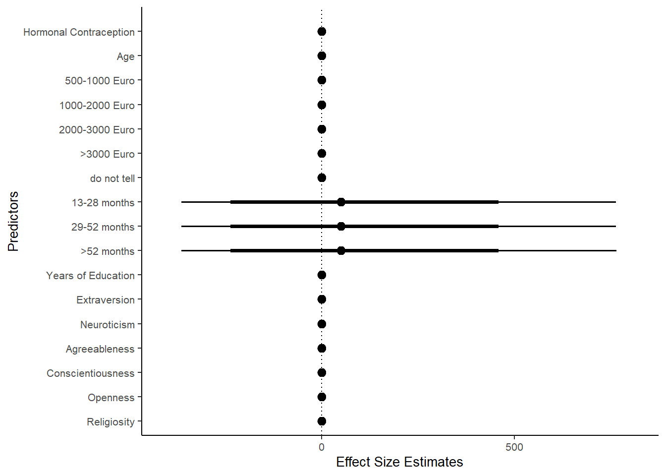
Sexual Satisfaction
Model
m_hc_sexsat_controlled = brm(satisfaction_sexual_intercourse ~ contraception_hormonal +
                             age + net_income + relationship_duration_factor +
                              education_years +
                              bfi_extra + bfi_neuro + bfi_agree + bfi_consc + bfi_open +
                              religiosity,
                data = data, family = gaussian(),
                file = "m_hc_sexsat_controlled_robust")
Summary
## Warning: Parts of the model have not converged (some Rhats are > 1.05). Be careful when analysing the results!
## We recommend running more iterations and/or setting stronger priors.
## Family: gaussian
## Links: mu = identity; sigma = identity
## Formula: satisfaction_sexual_intercourse ~ contraception_hormonal + age + net_income + relationship_duration_factor + education_years + bfi_extra + bfi_neuro + bfi_agree + bfi_consc + bfi_open + religiosity
## Data: data (Number of observations: 710)
## Draws: 4 chains, each with iter = 2000; warmup = 1000; thin = 1;
## total post-warmup draws = 4000
##
## Population-Level Effects:
## Estimate Est.Error l-90% CI u-90% CI Rhat Bulk_ESS
## Intercept 852.36 669.50 -311.85 1751.11 2.83 5
## contraception_hormonalyes 0.19 0.08 0.06 0.32 1.08 40
## age 0.01 0.01 -0.01 0.02 1.18 15
## net_incomeeuro_500_1000 0.05 0.09 -0.10 0.19 1.18 16
## net_incomeeuro_1000_2000 -0.01 0.13 -0.24 0.22 1.24 13
## net_incomeeuro_2000_3000 0.00 0.20 -0.30 0.33 1.19 15
## net_incomeeuro_gt_3000 -0.28 0.27 -0.75 0.15 1.05 63
## net_incomedont_tell 0.17 0.22 -0.19 0.54 1.12 30
## relationship_duration_factorPartnered_upto12months -849.16 669.45 -1748.14 315.21 2.83 5
## relationship_duration_factorPartnered_upto28months -849.17 669.45 -1748.01 315.05 2.83 5
## relationship_duration_factorPartnered_upto52months -849.40 669.45 -1748.29 314.80 2.83 5
## relationship_duration_factorPartnered_morethan52months -849.45 669.45 -1748.27 314.90 2.83 5
## education_years -0.00 0.01 -0.02 0.01 1.05 65
## bfi_extra 0.10 0.05 0.02 0.18 1.11 27
## bfi_neuro -0.08 0.06 -0.16 0.02 1.07 42
## bfi_agree 0.14 0.08 0.02 0.27 1.13 26
## bfi_consc 0.11 0.06 0.01 0.20 1.07 52
## bfi_open -0.09 0.06 -0.18 0.01 1.17 22
## religiosity 0.01 0.03 -0.04 0.05 1.29 14
## Tail_ESS
## Intercept NA
## contraception_hormonalyes NA
## age NA
## net_incomeeuro_500_1000 NA
## net_incomeeuro_1000_2000 NA
## net_incomeeuro_2000_3000 NA
## net_incomeeuro_gt_3000 NA
## net_incomedont_tell NA
## relationship_duration_factorPartnered_upto12months NA
## relationship_duration_factorPartnered_upto28months NA
## relationship_duration_factorPartnered_upto52months NA
## relationship_duration_factorPartnered_morethan52months NA
## education_years NA
## bfi_extra NA
## bfi_neuro NA
## bfi_agree NA
## bfi_consc NA
## bfi_open NA
## religiosity NA
##
## Family Specific Parameters:
## Estimate Est.Error l-90% CI u-90% CI Rhat Bulk_ESS Tail_ESS
## sigma 1.02 0.03 0.98 1.07 1.14 48 NA
##
## Draws were sampled using sampling(NUTS). For each parameter, Bulk_ESS
## and Tail_ESS are effective sample size measures, and Rhat is the potential
## scale reduction factor on split chains (at convergence, Rhat = 1).Comparison with ROPE
plot(equivalence_test(m_hc_sexsat_controlled, range = c(-0.11, 0.11), ci = 0.90,
                      parameters = "contraception"))
## Picking joint bandwidth of 0.0108## Warning: Removed 399 rows containing non-finite values (stat_density_ridges).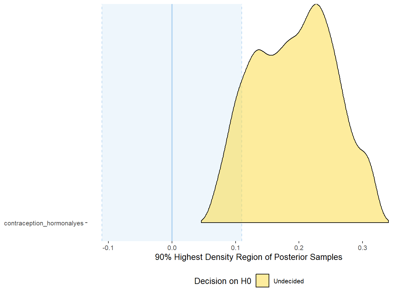
equivalence_test(m_hc_sexsat_controlled, range = c(-0.11, 0.11), ci = 0.90,
                      parameters = "contraception")
## # A tibble: 1 x 10
## Parameter CI ROPE_low ROPE_high ROPE_Percentage ROPE_Equivalence HDI_low HDI_high Effects Component
## <chr> <dbl> <dbl> <dbl> <dbl> <chr> <dbl> <dbl> <chr> <chr>
## 1 b_contraceptio~ 0.9 -0.11 0.11 0.109 Undecided 0.0656 0.320 fixed conditio~


Forest Plot for Effect Sizes
m_hc_sexsat_controlled %>%
  spread_draws(b_contraception_hormonalyes,
               b_age,
               b_net_incomeeuro_500_1000, b_net_incomeeuro_1000_2000,
               b_net_incomeeuro_2000_3000, b_net_incomeeuro_gt_3000, b_net_incomedont_tell,
               b_relationship_duration_factorPartnered_upto28months,
               b_relationship_duration_factorPartnered_upto52months,
               b_relationship_duration_factorPartnered_morethan52months,
               b_education_years,
               b_bfi_extra, b_bfi_neuro, b_bfi_agree, b_bfi_consc, b_bfi_open,
               b_religiosity) %>%
  pivot_longer(cols = c(b_contraception_hormonalyes,
                        b_age,
               b_net_incomeeuro_500_1000, b_net_incomeeuro_1000_2000,
               b_net_incomeeuro_2000_3000, b_net_incomeeuro_gt_3000, b_net_incomedont_tell,
               b_relationship_duration_factorPartnered_upto28months,
               b_relationship_duration_factorPartnered_upto52months,
               b_relationship_duration_factorPartnered_morethan52months,
               b_education_years,
               b_bfi_extra, b_bfi_neuro, b_bfi_agree, b_bfi_consc, b_bfi_open,
               b_religiosity),
               names_to = "condition",
               values_to = "r_condition") %>%
  mutate(condition_mean = r_condition,
         group = ifelse(condition %contains% "b_relationship_duration_factor",
                        "Relationship Duration",
                        ifelse(condition %contains% "b_net_income",
                               "Income",
                               NA)),
         group = ifelse(condition %contains% "b_contraception_hormonalyes",
                        "Contraception", group),
         condition = ifelse(condition %contains% "b_contraception_hormonalyes",
                        "Hormonal Contraception", condition),
         condition = ifelse(condition == "b_age", "Age",
                ifelse(condition == "b_net_incomeeuro_500_1000", "500-1000 Euro",
                ifelse(condition == "b_net_incomeeuro_1000_2000", "1000-2000 Euro",
                ifelse(condition == "b_net_incomeeuro_2000_3000", "2000-3000 Euro",
                ifelse(condition == "b_net_incomeeuro_gt_3000", ">3000 Euro",
                ifelse(condition == "b_net_incomedont_tell", "do not tell",
                ifelse(condition == "b_relationship_duration_factorPartnered_upto28months",
                       "13-28 months",
                ifelse(condition == "b_relationship_duration_factorPartnered_upto52months",
                       "29-52 months",
                ifelse(condition == "b_relationship_duration_factorPartnered_morethan52months",
                       ">52 months",
                ifelse(condition == "b_education_years", "Years of Education",
                ifelse(condition == "b_bfi_extra", "Extraversion",
                ifelse(condition == "b_bfi_neuro", "Neuroticism",
                ifelse(condition == "b_bfi_agree", "Agreeableness",
                ifelse(condition == "b_bfi_consc", "Conscientiousness",
                ifelse(condition == "b_bfi_open", "Openness",
                ifelse(condition == "b_religiosity", "Religiosity",
                       condition)))))))))))))))),
         group = ifelse(is.na(group), condition, group),
         condition = factor(condition, levels = rev(c("Hormonal Contraception", "Age",
                                        "500-1000 Euro", "1000-2000 Euro",
                                        "2000-3000 Euro", ">3000 Euro", "do not tell",
                                        "13-28 months", "29-52 months",
                                        ">52 months",
                                        "Years of Education",
                                        "Extraversion", "Neuroticism", "Agreeableness",
                                         "Conscientiousness","Openness","Religiosity"))),
         group = factor(group, levels = c("Contraception", "Age", "Income",
                                          "Relationship Duration","Years of Education",
                                          "Extraversion", "Neuroticism", "Agreeableness",
                                         "Conscientiousness","Openness","Religiosity"))) %>%
  ggplot(aes(y = condition,
             x = condition_mean,
             fill = stat(abs(x) < 0.11))) +
  stat_halfeye() +
  geom_vline(xintercept = c(-0.11, 0.11), linetype = "dotted") +
  apatheme +
  theme(legend.position = "none") +
  scale_fill_manual(values = c("gray80", "skyblue")) +
  labs(x = "Effect Size Estimates", y = "Predictors")
Libido
Model
Summary
## Family: gaussian
## Links: mu = identity; sigma = identity
## Formula: diary_libido_mean ~ contraception_hormonal + age + net_income + relationship_duration_factor + education_years + bfi_extra + bfi_neuro + bfi_agree + bfi_consc + bfi_open + religiosity
## Data: data (Number of observations: 910)
## Draws: 4 chains, each with iter = 2000; warmup = 1000; thin = 1;
## total post-warmup draws = 4000
##
## Population-Level Effects:
## Estimate Est.Error l-90% CI u-90% CI Rhat Bulk_ESS
## Intercept 0.27 0.27 -0.17 0.72 1.00 4476
## contraception_hormonalyes -0.02 0.04 -0.09 0.04 1.00 4296
## age 0.00 0.01 -0.01 0.01 1.00 3178
## net_incomeeuro_500_1000 0.09 0.05 0.01 0.17 1.00 3072
## net_incomeeuro_1000_2000 0.14 0.07 0.03 0.25 1.00 2401
## net_incomeeuro_2000_3000 0.15 0.10 -0.01 0.31 1.00 3091
## net_incomeeuro_gt_3000 -0.04 0.18 -0.33 0.26 1.00 3994
## net_incomedont_tell 0.13 0.13 -0.08 0.34 1.00 3293
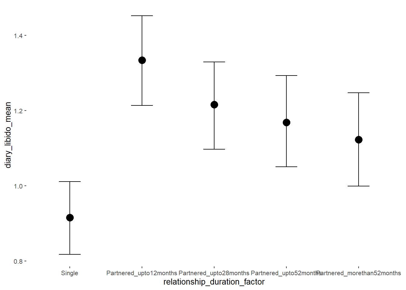
## relationship_duration_factorPartnered_upto12months 0.42 0.06 0.32 0.52 1.00 3251
## relationship_duration_factorPartnered_upto28months 0.30 0.06 0.21 0.39 1.00 3187
## relationship_duration_factorPartnered_upto52months 0.25 0.06 0.16 0.35 1.00 3194
## relationship_duration_factorPartnered_morethan52months 0.21 0.06 0.10 0.31 1.00 3320
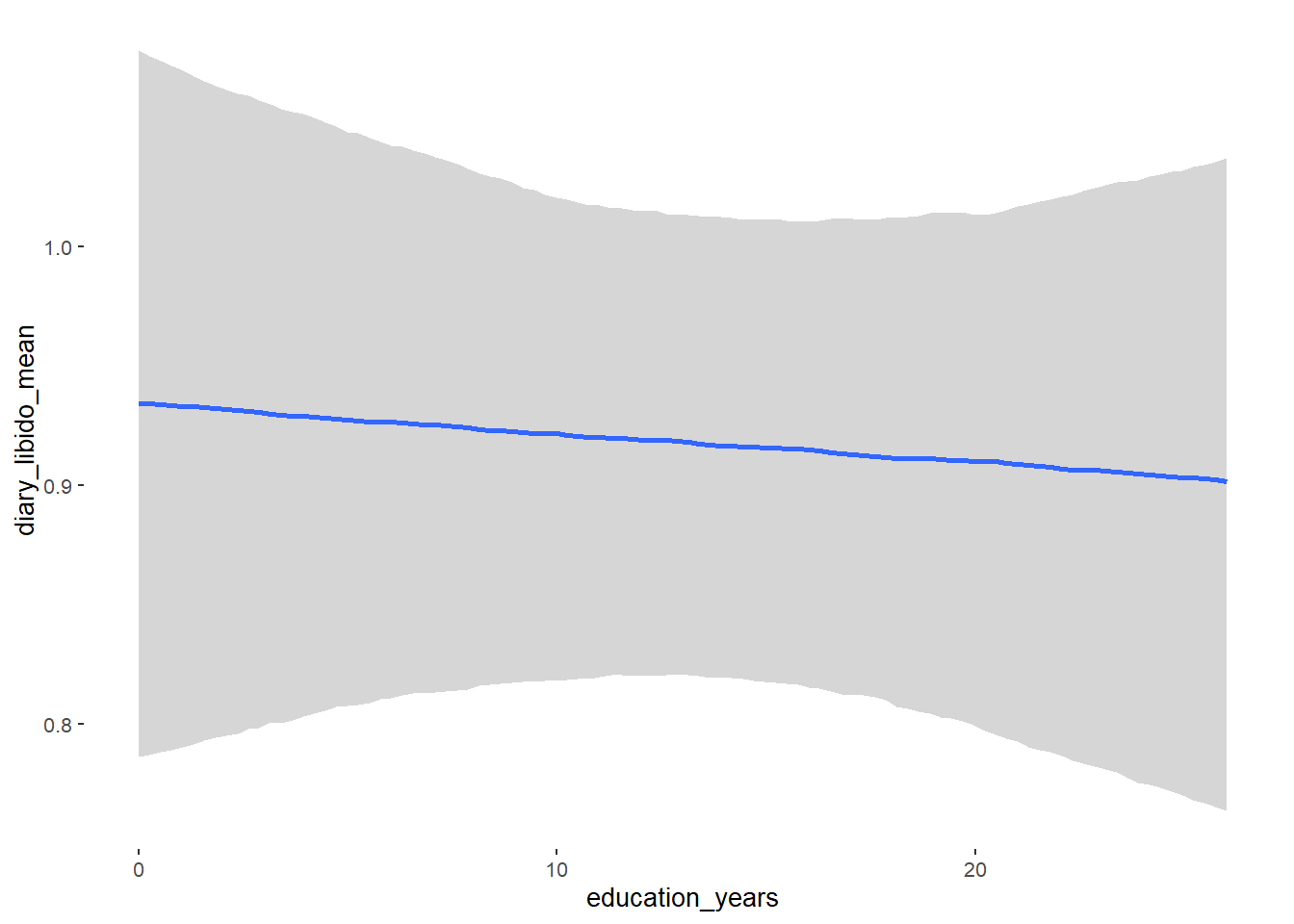
## education_years -0.00 0.00 -0.01 0.01 1.00 6750
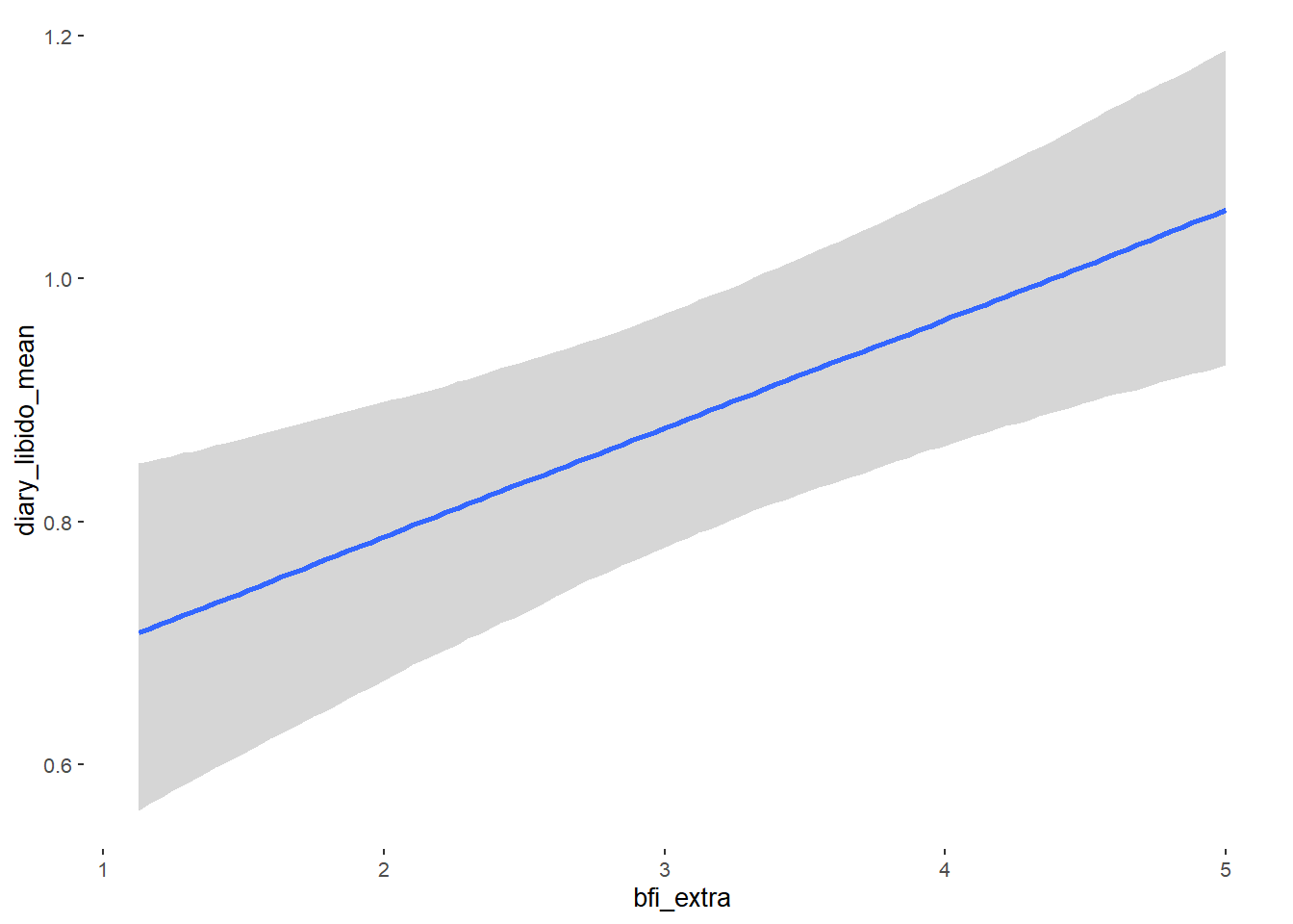
## bfi_extra 0.09 0.03 0.05 0.13 1.00 3806
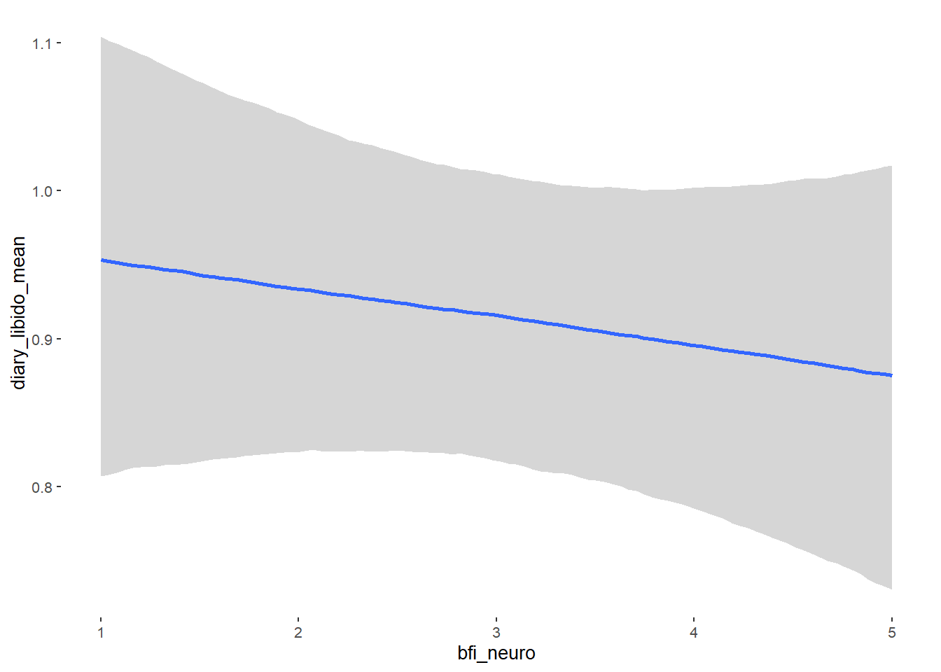
## bfi_neuro -0.02 0.03 -0.07 0.03 1.00 4144
## bfi_agree 0.08 0.03 0.02 0.13 1.00 3691
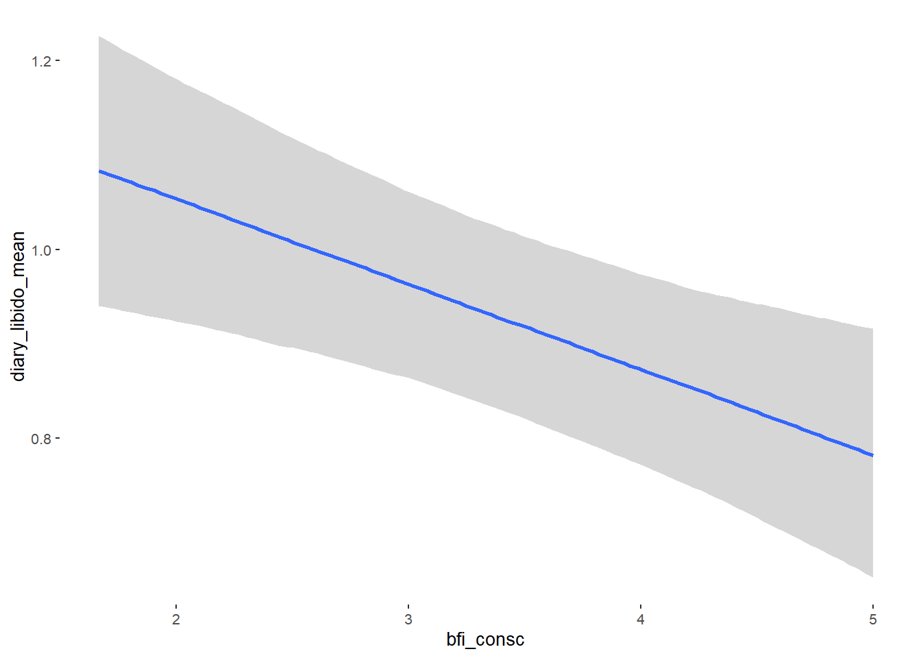
## bfi_consc -0.09 0.03 -0.14 -0.04 1.00 4333
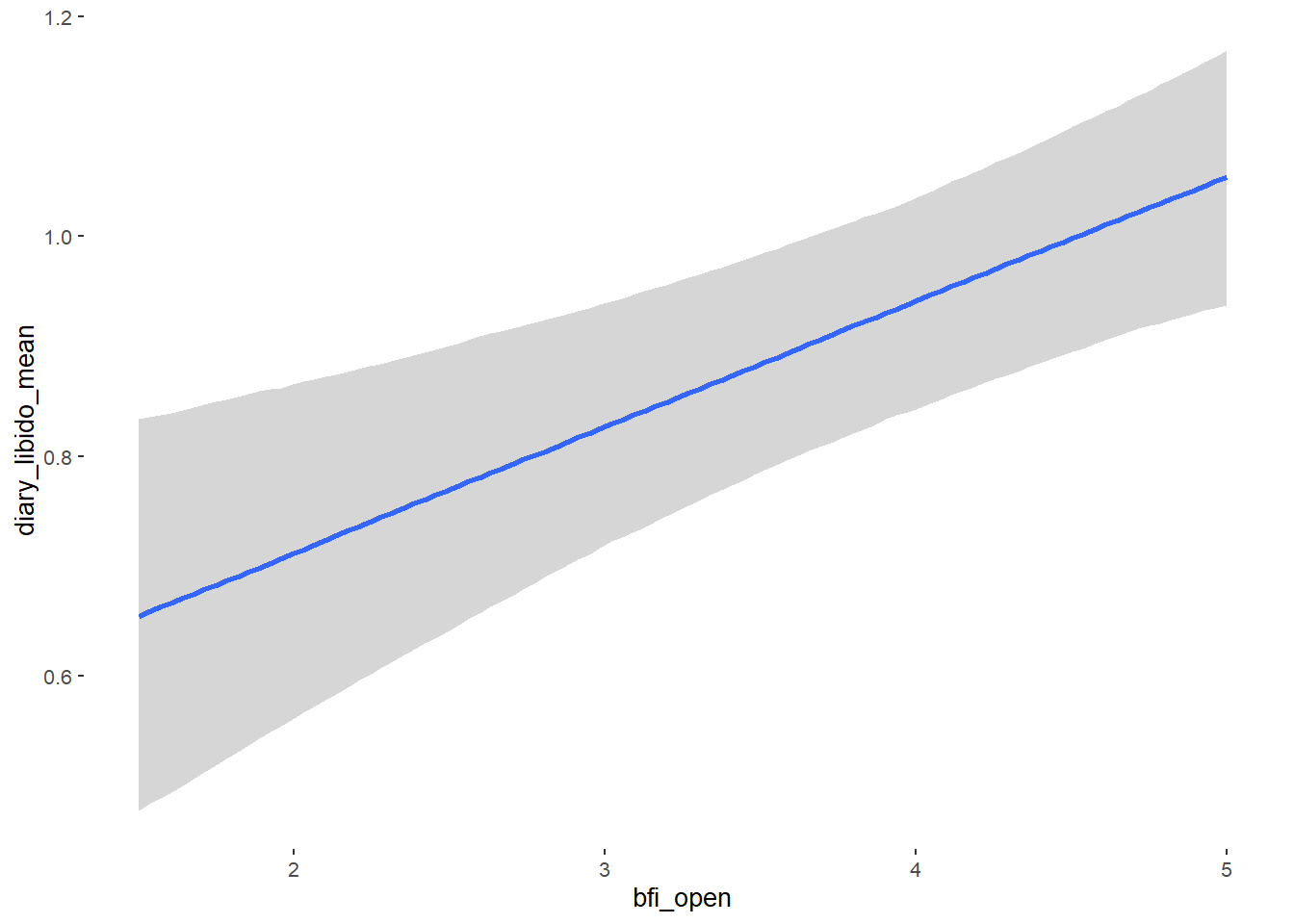
## bfi_open 0.11 0.03 0.06 0.17 1.00 4333
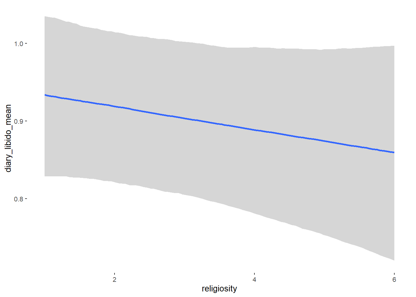
## religiosity -0.01 0.01 -0.04 0.01 1.00 4897
## Tail_ESS
## Intercept 2910
## contraception_hormonalyes 3003
## age 3047
## net_incomeeuro_500_1000 3148
## net_incomeeuro_1000_2000 2943
## net_incomeeuro_2000_3000 2944
## net_incomeeuro_gt_3000 2673
## net_incomedont_tell 3015
## relationship_duration_factorPartnered_upto12months 3161
## relationship_duration_factorPartnered_upto28months 2865
## relationship_duration_factorPartnered_upto52months 3012
## relationship_duration_factorPartnered_morethan52months 3191
## education_years 3328
## bfi_extra 2998
## bfi_neuro 3293
## bfi_agree 2940
## bfi_consc 3292
## bfi_open 2777
## religiosity 3206
##
## Family Specific Parameters:
## Estimate Est.Error l-90% CI u-90% CI Rhat Bulk_ESS Tail_ESS
## sigma 0.56 0.01 0.54 0.58 1.00 4843 3101
##
## Draws were sampled using sampling(NUTS). For each parameter, Bulk_ESS
## and Tail_ESS are effective sample size measures, and Rhat is the potential
## scale reduction factor on split chains (at convergence, Rhat = 1).Comparison with ROPE
plot(equivalence_test(m_hc_libido_controlled, range = c(-0.06, 0.06), ci = 0.90,
                      parameters = "contraception"))
## Picking joint bandwidth of 0.00551## Warning: Removed 399 rows containing non-finite values (stat_density_ridges).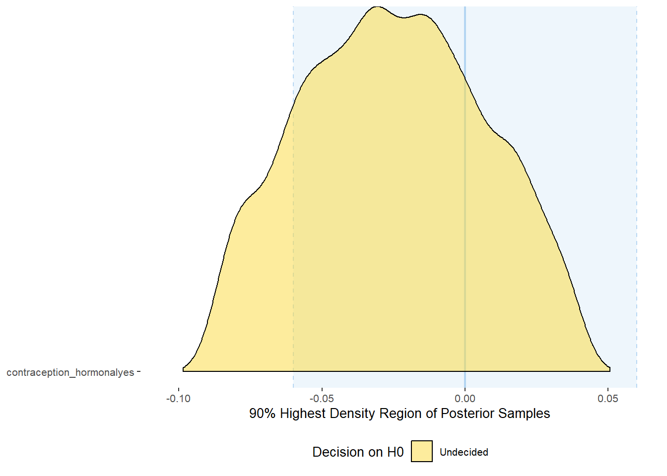
equivalence_test(m_hc_libido_controlled, range = c(-0.06, 0.06), ci = 0.90,
                      parameters = "contraception")
## # A tibble: 1 x 10
## Parameter CI ROPE_low ROPE_high ROPE_Percentage ROPE_Equivalence HDI_low HDI_high Effects Component
## <chr> <dbl> <dbl> <dbl> <dbl> <chr> <dbl> <dbl> <chr> <chr>
## 1 b_contraceptio~ 0.9 -0.06 0.06 0.845 Undecided -0.0887 0.0409 fixed conditio~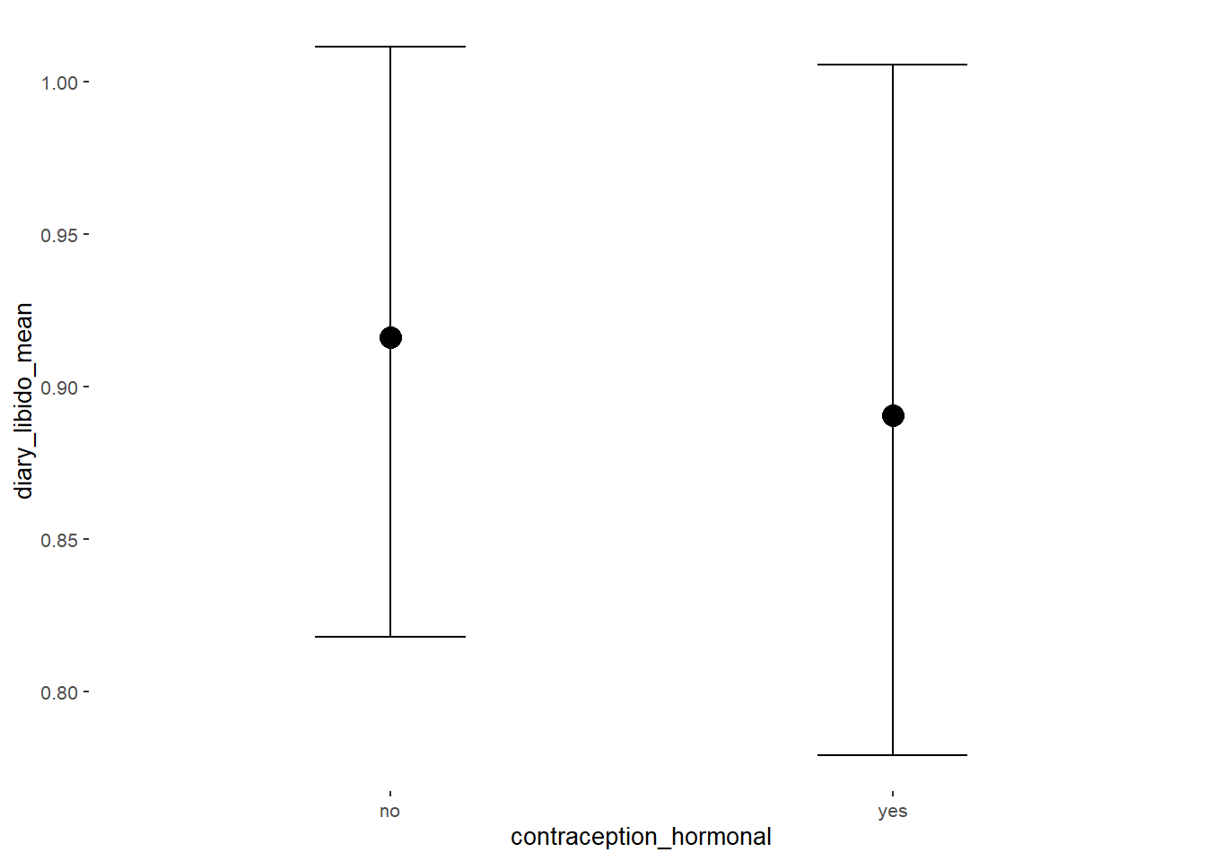
Forest Plot for Effect Sizes
m_hc_libido_controlled %>%
  spread_draws(b_contraception_hormonalyes,
               b_age,
               b_net_incomeeuro_500_1000, b_net_incomeeuro_1000_2000,
               b_net_incomeeuro_2000_3000, b_net_incomeeuro_gt_3000, b_net_incomedont_tell,
               b_relationship_duration_factorPartnered_upto28months,
               b_relationship_duration_factorPartnered_upto52months,
               b_relationship_duration_factorPartnered_morethan52months,
               b_education_years,
               b_bfi_extra, b_bfi_neuro, b_bfi_agree, b_bfi_consc, b_bfi_open,
               b_religiosity) %>%
  pivot_longer(cols = c(b_contraception_hormonalyes,
                        b_age,
               b_net_incomeeuro_500_1000, b_net_incomeeuro_1000_2000,
               b_net_incomeeuro_2000_3000, b_net_incomeeuro_gt_3000, b_net_incomedont_tell,
               b_relationship_duration_factorPartnered_upto28months,
               b_relationship_duration_factorPartnered_upto52months,
               b_relationship_duration_factorPartnered_morethan52months,
               b_education_years,
               b_bfi_extra, b_bfi_neuro, b_bfi_agree, b_bfi_consc, b_bfi_open,
               b_religiosity),
               names_to = "condition",
               values_to = "r_condition") %>%
  mutate(condition_mean = r_condition,
         group = ifelse(condition %contains% "b_relationship_duration_factor",
                        "Relationship Duration",
                        ifelse(condition %contains% "b_net_income",
                               "Income",
                               NA)),
         group = ifelse(condition %contains% "b_contraception_hormonalyes",
                        "Contraception", group),
         condition = ifelse(condition %contains% "b_contraception_hormonalyes",
                        "Hormonal Contraception", condition),
         condition = ifelse(condition == "b_age", "Age",
                ifelse(condition == "b_net_incomeeuro_500_1000", "500-1000 Euro",
                ifelse(condition == "b_net_incomeeuro_1000_2000", "1000-2000 Euro",
                ifelse(condition == "b_net_incomeeuro_2000_3000", "2000-3000 Euro",
                ifelse(condition == "b_net_incomeeuro_gt_3000", ">3000 Euro",
                ifelse(condition == "b_net_incomedont_tell", "do not tell",
                ifelse(condition == "b_relationship_duration_factorPartnered_upto28months",
                       "13-28 months",
                ifelse(condition == "b_relationship_duration_factorPartnered_upto52months",
                       "29-52 months",
                ifelse(condition == "b_relationship_duration_factorPartnered_morethan52months",
                       ">52 months",
                ifelse(condition == "b_education_years", "Years of Education",
                ifelse(condition == "b_bfi_extra", "Extraversion",
                ifelse(condition == "b_bfi_neuro", "Neuroticism",
                ifelse(condition == "b_bfi_agree", "Agreeableness",
                ifelse(condition == "b_bfi_consc", "Conscientiousness",
                ifelse(condition == "b_bfi_open", "Openness",
                ifelse(condition == "b_religiosity", "Religiosity",
                       condition)))))))))))))))),
         group = ifelse(is.na(group), condition, group),
         condition = factor(condition, levels = rev(c("Hormonal Contraception", "Age",
                                        "500-1000 Euro", "1000-2000 Euro",
                                        "2000-3000 Euro", ">3000 Euro", "do not tell",
                                        "13-28 months", "29-52 months",
                                        ">52 months",
                                        "Years of Education",
                                        "Extraversion", "Neuroticism", "Agreeableness",
                                         "Conscientiousness","Openness","Religiosity"))),
         group = factor(group, levels = c("Contraception", "Age", "Income",
                                          "Relationship Duration","Years of Education",
                                          "Extraversion", "Neuroticism", "Agreeableness",
                                         "Conscientiousness","Openness","Religiosity"))) %>%
  ggplot(aes(y = condition,
             x = condition_mean,
             fill = stat(abs(x) < 0.06))) +
  stat_halfeye() +
  geom_vline(xintercept = c(-0.06, 0.06), linetype = "dotted") +
  apatheme +
  theme(legend.position = "none") +
  scale_fill_manual(values = c("gray80", "skyblue")) +
  labs(x = "Effect Size Estimates", y = "Predictors")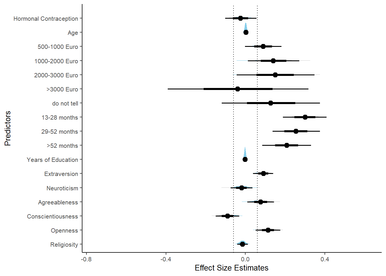
Sexual Frequency (Penetrative Intercourse)
Model
m_hc_sexfreqpen_controlled = brm(diary_sex_active_sex_sum ~
                        offset(log(number_of_days)) +
                        contraception_hormonal +
                        age + net_income + relationship_duration_factor +
                              education_years +
                              bfi_extra + bfi_neuro + bfi_agree + bfi_consc + bfi_open +
                              religiosity,
                data = data, family = poisson(),
                file = "m_hc_sexfreqpen_controlled_robust")
Summary
##  Family: poisson
##   Links: mu = log
## Formula: diary_sex_active_sex_sum ~ offset(log(number_of_days)) + contraception_hormonal + age + net_income + relationship_duration_factor + education_years + bfi_extra + bfi_neuro + bfi_agree + bfi_consc + bfi_open + religiosity
##    Data: data (Number of observations: 839)
##   Draws: 4 chains, each with iter = 2000; warmup = 1000; thin = 1;
##          total post-warmup draws = 4000
##
## Population-Level Effects:
##                                                        Estimate Est.Error l-90% CI u-90% CI Rhat Bulk_ESS
## Intercept                                                 -3.33      0.19    -3.64    -3.02 1.00     3797
## contraception_hormonalyes                                  0.13      0.03     0.08     0.17 1.00     3695
## age                                                       -0.00      0.00    -0.01     0.01 1.00     3364
## net_incomeeuro_500_1000                                    0.14      0.03     0.09     0.20 1.00     2738
## net_incomeeuro_1000_2000                                   0.15      0.05     0.08     0.23 1.00     2541
## net_incomeeuro_2000_3000                                   0.43      0.06     0.34     0.53 1.00     2749
## net_incomeeuro_gt_3000                                     0.05      0.11    -0.14     0.23 1.00     3661
## net_incomedont_tell                                        0.46      0.08     0.34     0.59 1.00     3269
## relationship_duration_factorPartnered_upto12months         1.34      0.04     1.26     1.41 1.00     1999
## relationship_duration_factorPartnered_upto28months         1.20      0.04     1.13     1.27 1.00     1983
## relationship_duration_factorPartnered_upto52months         0.96      0.05     0.87     1.04 1.00     2222
## relationship_duration_factorPartnered_morethan52months     0.94      0.05     0.86     1.03 1.00     2336
## education_years                                           -0.01      0.00    -0.02    -0.01 1.00     6946
## bfi_extra                                                  0.01      0.02    -0.01     0.04 1.00     3961
## bfi_neuro                                                 -0.01      0.02    -0.04     0.03 1.00     3594
## bfi_agree                                                  0.08      0.02     0.05     0.12 1.00     3603
## bfi_consc                                                 -0.00      0.02    -0.04     0.03 1.00     4598
## bfi_open                                                   0.04      0.02    -0.00     0.07 1.00     4100
## religiosity                                               -0.02      0.01    -0.04    -0.00 1.00     4343
##                                                        Tail_ESS
## Intercept                                                  3224
## contraception_hormonalyes                                  3008
## age                                                        3179
## net_incomeeuro_500_1000                                    2725
## net_incomeeuro_1000_2000                                   2658
## net_incomeeuro_2000_3000                                   3009
## net_incomeeuro_gt_3000                                     3008
## net_incomedont_tell                                        2846
## relationship_duration_factorPartnered_upto12months         3039
## relationship_duration_factorPartnered_upto28months         3068
## relationship_duration_factorPartnered_upto52months         2773
## relationship_duration_factorPartnered_morethan52months     2765
## education_years                                            3211
## bfi_extra                                                  3172
## bfi_neuro                                                  3131
## bfi_agree                                                  2756
## bfi_consc                                                  2968
## bfi_open                                                   3040
## religiosity                                                2910
##
## Draws were sampled using sampling(NUTS). For each parameter, Bulk_ESS
## and Tail_ESS are effective sample size measures, and Rhat is the potential
## scale reduction factor on split chains (at convergence, Rhat = 1).
Comparison with ROPE
plot(equivalence_test(m_hc_sexfreqpen_controlled, range = c(-0.05, 0.05), ci = 0.90,
                      parameters = "contraception"))
## Picking joint bandwidth of 0.00384## Warning: Removed 399 rows containing non-finite values (stat_density_ridges).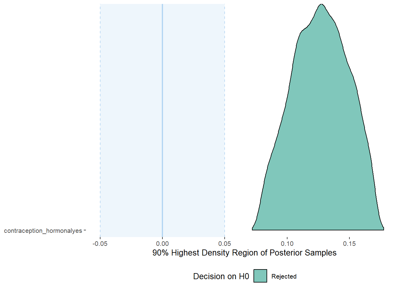
equivalence_test(m_hc_sexfreqpen_controlled, range = c(-0.05, 0.05), ci = 0.90,
                      parameters = "contraception")
## # A tibble: 1 x 10
## Parameter CI ROPE_low ROPE_high ROPE_Percentage ROPE_Equivalence HDI_low HDI_high Effects Component
## <chr> <dbl> <dbl> <dbl> <dbl> <chr> <dbl> <dbl> <chr> <chr>
## 1 b_contraceptio~ 0.9 -0.05 0.05 0 Rejected 0.0788 0.171 fixed conditio~Plots
conditional_effects(m_hc_sexfreqpen_controlled,
                    effects = "contraception_hormonal",
                    conditions = data.frame(number_of_days = 1))
Forest Plot for Effect Sizes
m_hc_sexfreqpen_controlled %>%
  spread_draws(b_contraception_hormonalyes,
               b_age,
               b_net_incomeeuro_500_1000, b_net_incomeeuro_1000_2000,
               b_net_incomeeuro_2000_3000, b_net_incomeeuro_gt_3000, b_net_incomedont_tell,
               b_relationship_duration_factorPartnered_upto28months,
               b_relationship_duration_factorPartnered_upto52months,
               b_relationship_duration_factorPartnered_morethan52months,
               b_education_years,
               b_bfi_extra, b_bfi_neuro, b_bfi_agree, b_bfi_consc, b_bfi_open,
               b_religiosity) %>%
  pivot_longer(cols = c(b_contraception_hormonalyes,
                        b_age,
               b_net_incomeeuro_500_1000, b_net_incomeeuro_1000_2000,
               b_net_incomeeuro_2000_3000, b_net_incomeeuro_gt_3000, b_net_incomedont_tell,
               b_relationship_duration_factorPartnered_upto28months,
               b_relationship_duration_factorPartnered_upto52months,
               b_relationship_duration_factorPartnered_morethan52months,
               b_education_years,
               b_bfi_extra, b_bfi_neuro, b_bfi_agree, b_bfi_consc, b_bfi_open,
               b_religiosity),
               names_to = "condition",
               values_to = "r_condition") %>%
  mutate(condition_mean = r_condition,
         group = ifelse(condition %contains% "b_relationship_duration_factor",
                        "Relationship Duration",
                        ifelse(condition %contains% "b_net_income",
                               "Income",
                               NA)),
         group = ifelse(condition %contains% "b_contraception_hormonalyes",
                        "Contraception", group),
         condition = ifelse(condition %contains% "b_contraception_hormonalyes",
                        "Hormonal Contraception", condition),
         condition = ifelse(condition == "b_age", "Age",
                ifelse(condition == "b_net_incomeeuro_500_1000", "500-1000 Euro",
                ifelse(condition == "b_net_incomeeuro_1000_2000", "1000-2000 Euro",
                ifelse(condition == "b_net_incomeeuro_2000_3000", "2000-3000 Euro",
                ifelse(condition == "b_net_incomeeuro_gt_3000", ">3000 Euro",
                ifelse(condition == "b_net_incomedont_tell", "do not tell",
                ifelse(condition == "b_relationship_duration_factorPartnered_upto28months",
                       "13-28 months",
                ifelse(condition == "b_relationship_duration_factorPartnered_upto52months",
                       "29-52 months",
                ifelse(condition == "b_relationship_duration_factorPartnered_morethan52months",
                       ">52 months",
                ifelse(condition == "b_education_years", "Years of Education",
                ifelse(condition == "b_bfi_extra", "Extraversion",
                ifelse(condition == "b_bfi_neuro", "Neuroticism",
                ifelse(condition == "b_bfi_agree", "Agreeableness",
                ifelse(condition == "b_bfi_consc", "Conscientiousness",
                ifelse(condition == "b_bfi_open", "Openness",
                ifelse(condition == "b_religiosity", "Religiosity",
                       condition)))))))))))))))),
         group = ifelse(is.na(group), condition, group),
         condition = factor(condition, levels = rev(c("Hormonal Contraception", "Age",
                                        "500-1000 Euro", "1000-2000 Euro",
                                        "2000-3000 Euro", ">3000 Euro", "do not tell",
                                        "13-28 months", "29-52 months",
                                        ">52 months",
                                        "Years of Education",
                                        "Extraversion", "Neuroticism", "Agreeableness",
                                         "Conscientiousness","Openness","Religiosity"))),
         group = factor(group, levels = c("Contraception", "Age", "Income",
                                          "Relationship Duration","Years of Education",
                                          "Extraversion", "Neuroticism", "Agreeableness",
                                         "Conscientiousness","Openness","Religiosity"))) %>%
  ggplot(aes(y = condition,
             x = condition_mean,
             fill = stat(abs(x) < 0.05))) +
  stat_halfeye() +
  geom_vline(xintercept = c(-0.05, 0.05), linetype = "dotted") +
  apatheme +
  theme(legend.position = "none") +
  scale_fill_manual(values = c("gray80", "skyblue")) +
  labs(x = "Effect Size Estimates", y = "Predictors")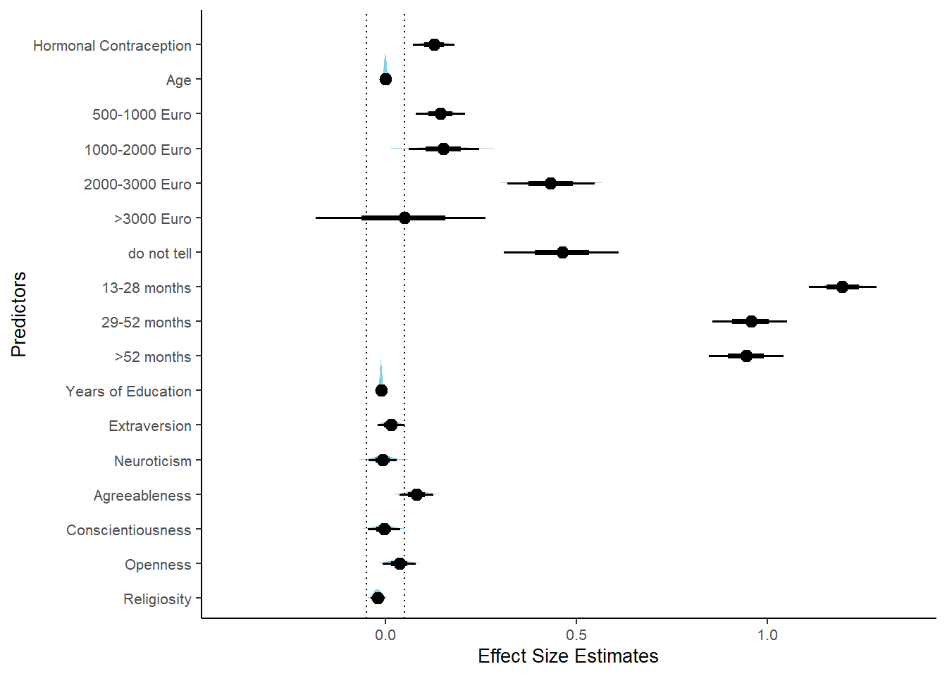
Masturabation Frequency
Model
m_hc_masfreq_controlled = brm(diary_masturbation_sum ~
                        offset(log(number_of_days)) +
                        contraception_hormonal +
                        age + net_income + relationship_duration_factor +
                              education_years +
                              bfi_extra + bfi_neuro + bfi_agree + bfi_consc + bfi_open +
                              religiosity,
                data = data, family = poisson(),
                file = "m_hc_masfreq_controlled_robust")
Summary
##  Family: poisson
##   Links: mu = log
## Formula: diary_masturbation_sum ~ offset(log(number_of_days)) + contraception_hormonal + age + net_income + relationship_duration_factor + education_years + bfi_extra + bfi_neuro + bfi_agree + bfi_consc + bfi_open + religiosity
##    Data: data (Number of observations: 839)
##   Draws: 4 chains, each with iter = 2000; warmup = 1000; thin = 1;
##          total post-warmup draws = 4000
##
## Population-Level Effects:
##                                                        Estimate Est.Error l-90% CI u-90% CI Rhat Bulk_ESS
## Intercept                                                 -1.68      0.19    -2.01    -1.37 1.00     4868
## contraception_hormonalyes                                 -0.35      0.03    -0.40    -0.30 1.00     4571
## age                                                       -0.00      0.00    -0.01     0.00 1.00     4025
## net_incomeeuro_500_1000                                    0.18      0.03     0.12     0.23 1.00     2981
## net_incomeeuro_1000_2000                                   0.20      0.05     0.12     0.28 1.00     2711
## net_incomeeuro_2000_3000                                  -0.02      0.08    -0.15     0.10 1.00     3262
## net_incomeeuro_gt_3000                                    -0.17      0.14    -0.41     0.06 1.00     4590
## net_incomedont_tell                                       -0.22      0.11    -0.40    -0.05 1.00     4038
## relationship_duration_factorPartnered_upto12months        -0.21      0.04    -0.28    -0.15 1.00     3947
## relationship_duration_factorPartnered_upto28months        -0.17      0.04    -0.23    -0.10 1.00     3959
## relationship_duration_factorPartnered_upto52months        -0.29      0.04    -0.36    -0.22 1.00     4035
## relationship_duration_factorPartnered_morethan52months    -0.45      0.04    -0.52    -0.38 1.00     3655
## education_years                                            0.00      0.00    -0.00     0.01 1.00     8241
## bfi_extra                                                 -0.03      0.02    -0.06     0.00 1.00     4570
## bfi_neuro                                                 -0.01      0.02    -0.04     0.02 1.00     4061
## bfi_agree                                                  0.00      0.02    -0.04     0.04 1.00     4591
## bfi_consc                                                 -0.20      0.02    -0.23    -0.17 1.00     5059
## bfi_open                                                   0.21      0.02     0.17     0.25 1.00     5451
## religiosity                                               -0.05      0.01    -0.07    -0.04 1.00     5192
##                                                        Tail_ESS
## Intercept                                                  3108
## contraception_hormonalyes                                  3352
## age                                                        2837
## net_incomeeuro_500_1000                                    2962
## net_incomeeuro_1000_2000                                   2814
## net_incomeeuro_2000_3000                                   3012
## net_incomeeuro_gt_3000                                     3336
## net_incomedont_tell                                        2804
## relationship_duration_factorPartnered_upto12months         3046
## relationship_duration_factorPartnered_upto28months         3115
## relationship_duration_factorPartnered_upto52months         2804
## relationship_duration_factorPartnered_morethan52months     3208
## education_years                                            3059
## bfi_extra                                                  3306
## bfi_neuro                                                  3165
## bfi_agree                                                  3149
## bfi_consc                                                  3354
## bfi_open                                                   3300
## religiosity                                                3090
##
## Draws were sampled using sampling(NUTS). For each parameter, Bulk_ESS
## and Tail_ESS are effective sample size measures, and Rhat is the potential
## scale reduction factor on split chains (at convergence, Rhat = 1).
Comparison with ROPE
plot(equivalence_test(m_hc_masfreq_controlled, range = c(-0.05, 0.05), ci = 0.90,
                      parameters = "contraception"))
## Picking joint bandwidth of 0.00416## Warning: Removed 399 rows containing non-finite values (stat_density_ridges).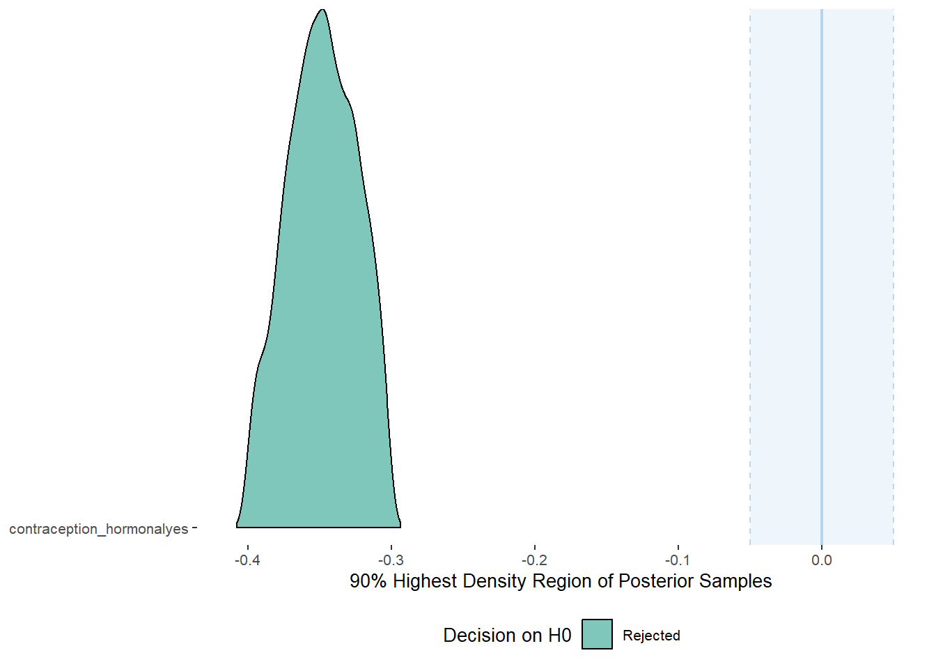
equivalence_test(m_hc_masfreq_controlled, range = c(-0.05, 0.05), ci = 0.90,
                      parameters = "contraception")
## # A tibble: 1 x 10
## Parameter CI ROPE_low ROPE_high ROPE_Percentage ROPE_Equivalence HDI_low HDI_high Effects Component
## <chr> <dbl> <dbl> <dbl> <dbl> <chr> <dbl> <dbl> <chr> <chr>
## 1 b_contraceptio~ 0.9 -0.05 0.05 0 Rejected -0.400 -0.301 fixed conditio~Plots
conditional_effects(m_hc_masfreq_controlled,
                    effects = "contraception_hormonal",
                    conditions = data.frame(number_of_days = 1))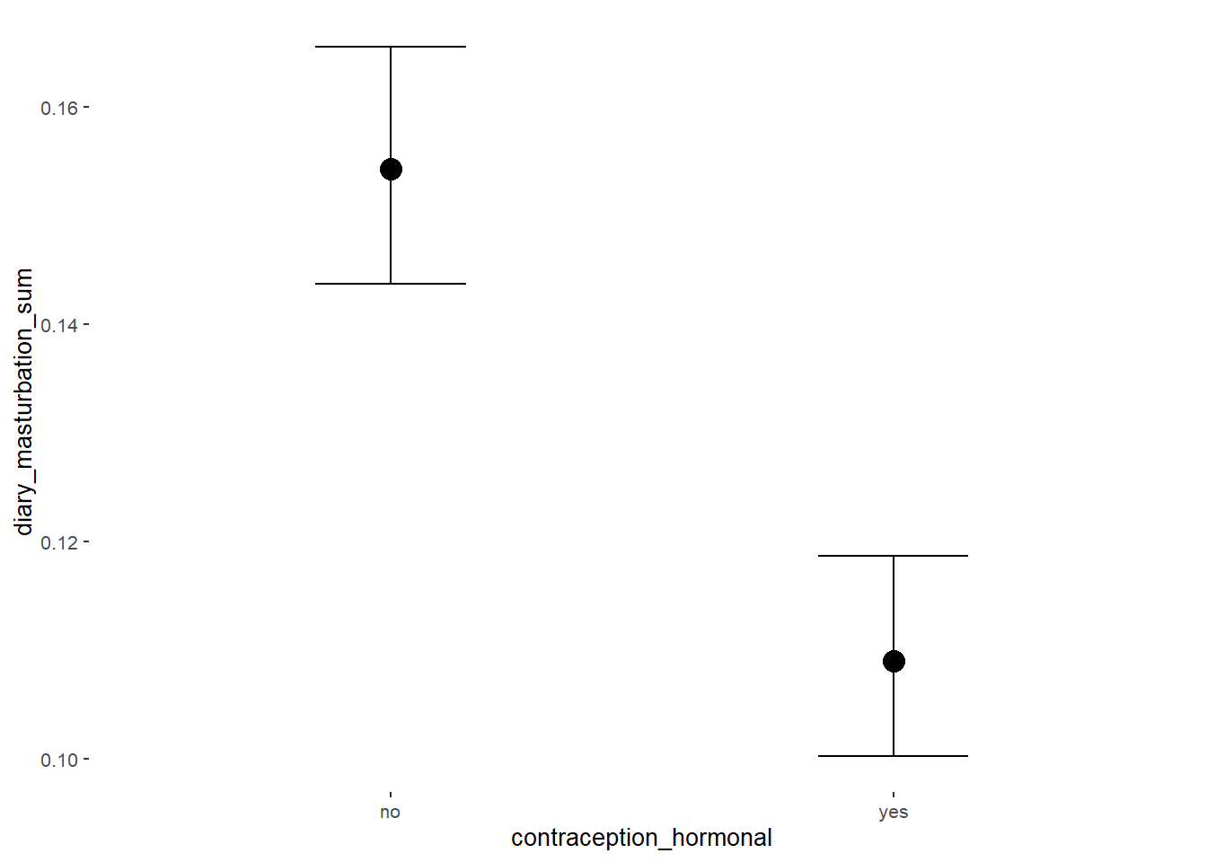
Forest Plot for Effect Sizes
m_hc_masfreq_controlled %>%
  spread_draws(b_contraception_hormonalyes,
               b_age,
               b_net_incomeeuro_500_1000, b_net_incomeeuro_1000_2000,
               b_net_incomeeuro_2000_3000, b_net_incomeeuro_gt_3000, b_net_incomedont_tell,
               b_relationship_duration_factorPartnered_upto28months,
               b_relationship_duration_factorPartnered_upto52months,
               b_relationship_duration_factorPartnered_morethan52months,
               b_education_years,
               b_bfi_extra, b_bfi_neuro, b_bfi_agree, b_bfi_consc, b_bfi_open,
               b_religiosity) %>%
  pivot_longer(cols = c(b_contraception_hormonalyes,
                        b_age,
               b_net_incomeeuro_500_1000, b_net_incomeeuro_1000_2000,
               b_net_incomeeuro_2000_3000, b_net_incomeeuro_gt_3000, b_net_incomedont_tell,
               b_relationship_duration_factorPartnered_upto28months,
               b_relationship_duration_factorPartnered_upto52months,
               b_relationship_duration_factorPartnered_morethan52months,
               b_education_years,
               b_bfi_extra, b_bfi_neuro, b_bfi_agree, b_bfi_consc, b_bfi_open,
               b_religiosity),
               names_to = "condition",
               values_to = "r_condition") %>%
  mutate(condition_mean = r_condition,
         group = ifelse(condition %contains% "b_relationship_duration_factor",
                        "Relationship Duration",
                        ifelse(condition %contains% "b_net_income",
                               "Income",
                               NA)),
         group = ifelse(condition %contains% "b_contraception_hormonalyes",
                        "Contraception", group),
         condition = ifelse(condition %contains% "b_contraception_hormonalyes",
                        "Hormonal Contraception", condition),
         condition = ifelse(condition == "b_age", "Age",
                ifelse(condition == "b_net_incomeeuro_500_1000", "500-1000 Euro",
                ifelse(condition == "b_net_incomeeuro_1000_2000", "1000-2000 Euro",
                ifelse(condition == "b_net_incomeeuro_2000_3000", "2000-3000 Euro",
                ifelse(condition == "b_net_incomeeuro_gt_3000", ">3000 Euro",
                ifelse(condition == "b_net_incomedont_tell", "do not tell",
                ifelse(condition == "b_relationship_duration_factorPartnered_upto28months",
                       "13-28 months",
                ifelse(condition == "b_relationship_duration_factorPartnered_upto52months",
                       "29-52 months",
                ifelse(condition == "b_relationship_duration_factorPartnered_morethan52months",
                       ">52 months",
                ifelse(condition == "b_education_years", "Years of Education",
                ifelse(condition == "b_bfi_extra", "Extraversion",
                ifelse(condition == "b_bfi_neuro", "Neuroticism",
                ifelse(condition == "b_bfi_agree", "Agreeableness",
                ifelse(condition == "b_bfi_consc", "Conscientiousness",
                ifelse(condition == "b_bfi_open", "Openness",
                ifelse(condition == "b_religiosity", "Religiosity",
                       condition)))))))))))))))),
         group = ifelse(is.na(group), condition, group),
         condition = factor(condition, levels = rev(c("Hormonal Contraception", "Age",
                                        "500-1000 Euro", "1000-2000 Euro",
                                        "2000-3000 Euro", ">3000 Euro", "do not tell",
                                        "13-28 months", "29-52 months",
                                        ">52 months",
                                        "Years of Education",
                                        "Extraversion", "Neuroticism", "Agreeableness",
                                         "Conscientiousness","Openness","Religiosity"))),
         group = factor(group, levels = c("Contraception", "Age", "Income",
                                          "Relationship Duration","Years of Education",
                                          "Extraversion", "Neuroticism", "Agreeableness",
                                         "Conscientiousness","Openness","Religiosity"))) %>%
  ggplot(aes(y = condition,
             x = condition_mean,
             fill = stat(abs(x) < 0.05))) +
  stat_halfeye() +
  geom_vline(xintercept = c(-0.05, 0.05), linetype = "dotted") +
  apatheme +
  theme(legend.position = "none") +
  scale_fill_manual(values = c("gray80", "skyblue")) +
  labs(x = "Effect Size Estimates", y = "Predictors")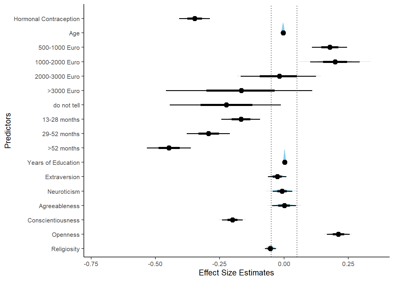
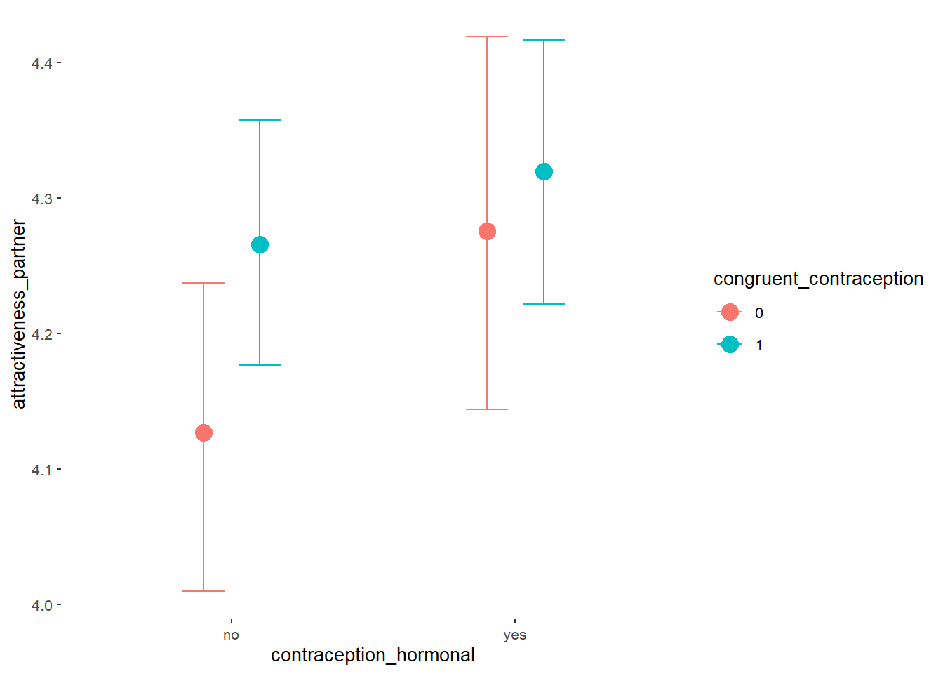
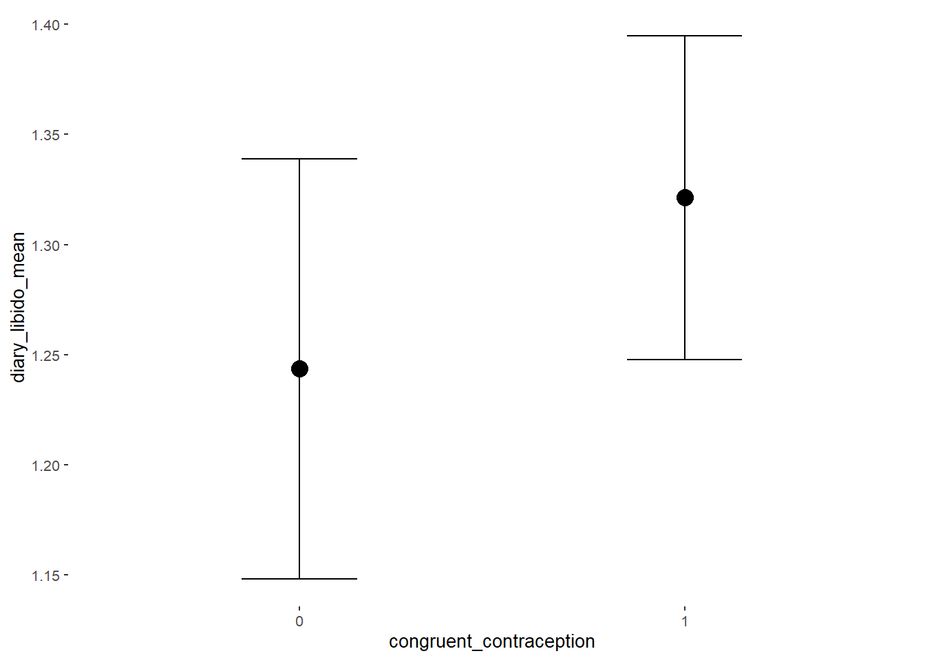
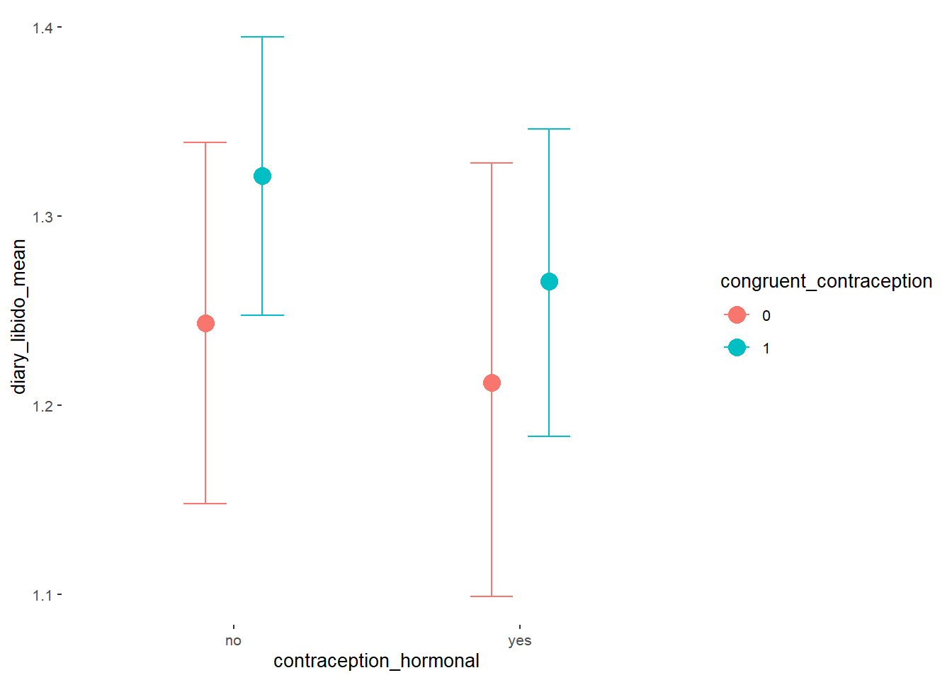
Effects of (In)Congruenct HC Use
Attractiveness of Partner
Model
Summary
##  Family: gaussian
##   Links: mu = identity; sigma = identity
## Formula: attractiveness_partner ~ contraception_hormonal * congruent_contraception
##    Data: data (Number of observations: 710)
##   Draws: 4 chains, each with iter = 2000; warmup = 1000; thin = 1;
##          total post-warmup draws = 4000
##
## Population-Level Effects:
##                                                    Estimate Est.Error l-90% CI u-90% CI Rhat Bulk_ESS
## Intercept                                              4.13      0.06     4.03     4.22 1.00     2505
## contraception_hormonalyes                              0.15      0.09     0.00     0.30 1.00     2166
## congruent_contraception1                               0.14      0.07     0.02     0.26 1.00     2448
## contraception_hormonalyes:congruent_contraception1    -0.10      0.11    -0.28     0.09 1.00     1917
##                                                    Tail_ESS
## Intercept                                              2989
## contraception_hormonalyes                              2464
## congruent_contraception1                               2750
## contraception_hormonalyes:congruent_contraception1     2333
##
## Family Specific Parameters:
##       Estimate Est.Error l-90% CI u-90% CI Rhat Bulk_ESS Tail_ESS
## sigma     0.73      0.02     0.69     0.76 1.00     3711     2781
##
## Draws were sampled using sampling(NUTS). For each parameter, Bulk_ESS
## and Tail_ESS are effective sample size measures, and Rhat is the potential
## scale reduction factor on split chains (at convergence, Rhat = 1).
Comparison with ROPE
plot(equivalence_test(m_congruency_atrr, range = c(-0.07, 0.07), ci = 0.90,
                      parameters = "contraception"))
## Possible multicollinearity between b_contraception_hormonalyes:congruent_contraception1 and b_contraception_hormonalyes (r = 0.8). This might lead to inappropriate results. See 'Details' in '?equivalence_test'.## Picking joint bandwidth of 0.0129## Warning: Removed 1197 rows containing non-finite values (stat_density_ridges).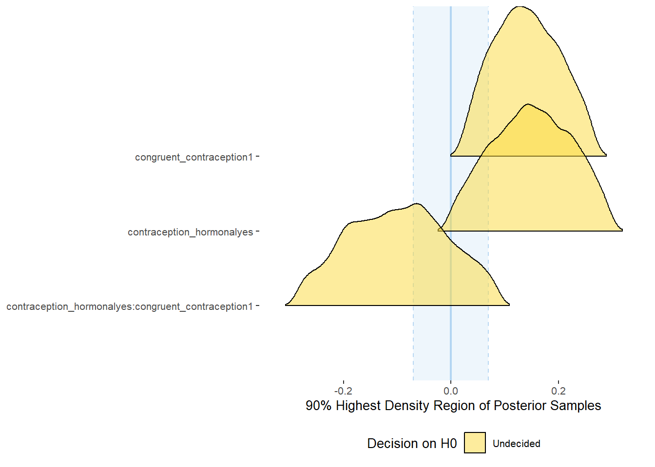
equivalence_test(m_congruency_atrr, range = c(-0.07, 0.07), ci = 0.90,
                      parameters = "contraception")
## Possible multicollinearity between b_contraception_hormonalyes:congruent_contraception1 and b_contraception_hormonalyes (r = 0.8). This might lead to inappropriate results. See 'Details' in '?equivalence_test'.## # A tibble: 3 x 10
## Parameter CI ROPE_low ROPE_high ROPE_Percentage ROPE_Equivalence HDI_low HDI_high Effects Component
## <chr> <dbl> <dbl> <dbl> <dbl> <chr> <dbl> <dbl> <chr> <chr>
## 1 b_contracepti~ 0.9 -0.07 0.07 0.157 Undecided -9.35e-4 0.296 fixed conditio~
## 2 b_congruent_c~ 0.9 -0.07 0.07 0.135 Undecided 2.27e-2 0.266 fixed conditio~
## 3 b_contracepti~ 0.9 -0.07 0.07 0.377 Undecided -2.85e-1 0.0872 fixed conditio~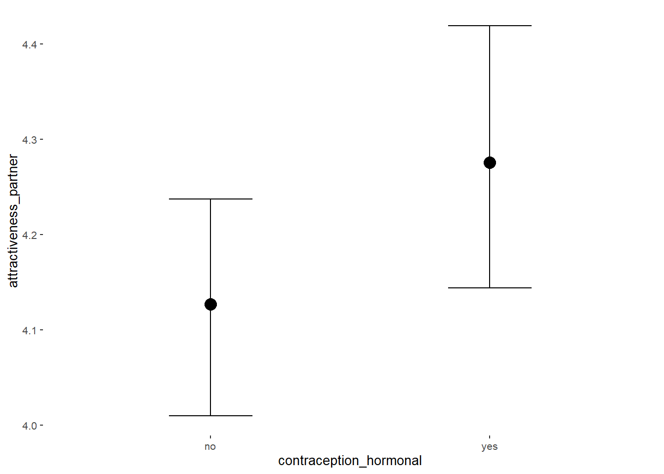
Forest Plot for Effect Sizes
m_congruency_atrr %>%
  spread_draws(b_contraception_hormonalyes, b_congruent_contraception1,
               `b_contraception_hormonalyes:congruent_contraception1`) %>%
  pivot_longer(cols = c(b_contraception_hormonalyes, b_congruent_contraception1,
               `b_contraception_hormonalyes:congruent_contraception1`),
               names_to = "condition",
               values_to = "r_condition") %>%
  mutate(condition_mean = r_condition,
         group = ifelse(condition %contains% "ontraception",
                        "Contraception", NA),
         condition = ifelse(condition == "b_contraception_hormonalyes",
                        "Hormonal Contraception",
                     ifelse(condition == "b_congruent_contraception1",
                            "Congruent Contraception",
                     ifelse(condition == "b_contraception_hormonalyes:congruent_contraception1",
                            "Interaction Hormonal Contracpetion and Congruent Contraception",
                            condition))),
         condition = factor(condition, levels = rev(c("Hormonal Contraception",
                                            "Congruent Contraception",
                                            "Interaction Hormonal Contracpetion and Congruent Contraception")))) %>%
  ggplot(aes(y = condition,
             x = condition_mean,
             fill = stat(abs(x) < 0.07))) +
  stat_halfeye() +
  geom_vline(xintercept = c(-0.07, 0.07), linetype = "dotted") +
  apatheme +
  theme(legend.position = "none") +
  scale_fill_manual(values = c("gray80", "skyblue")) +
  labs(x = "Effect Size Estimates", y = "Predictors") +
  xlim (-0.6, 0.6)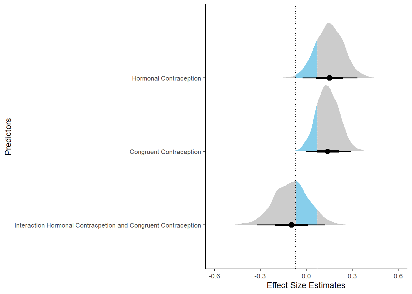
Relationship Satisfaction
Model
Summary
## Family: gaussian
## Links: mu = identity; sigma = identity
## Formula: relationship_satisfaction ~ contraception_hormonal * congruent_contraception
## Data: data (Number of observations: 710)
## Draws: 4 chains, each with iter = 2000; warmup = 1000; thin = 1;
## total post-warmup draws = 4000
##
## Population-Level Effects:
## Estimate Est.Error l-90% CI u-90% CI Rhat Bulk_ESS
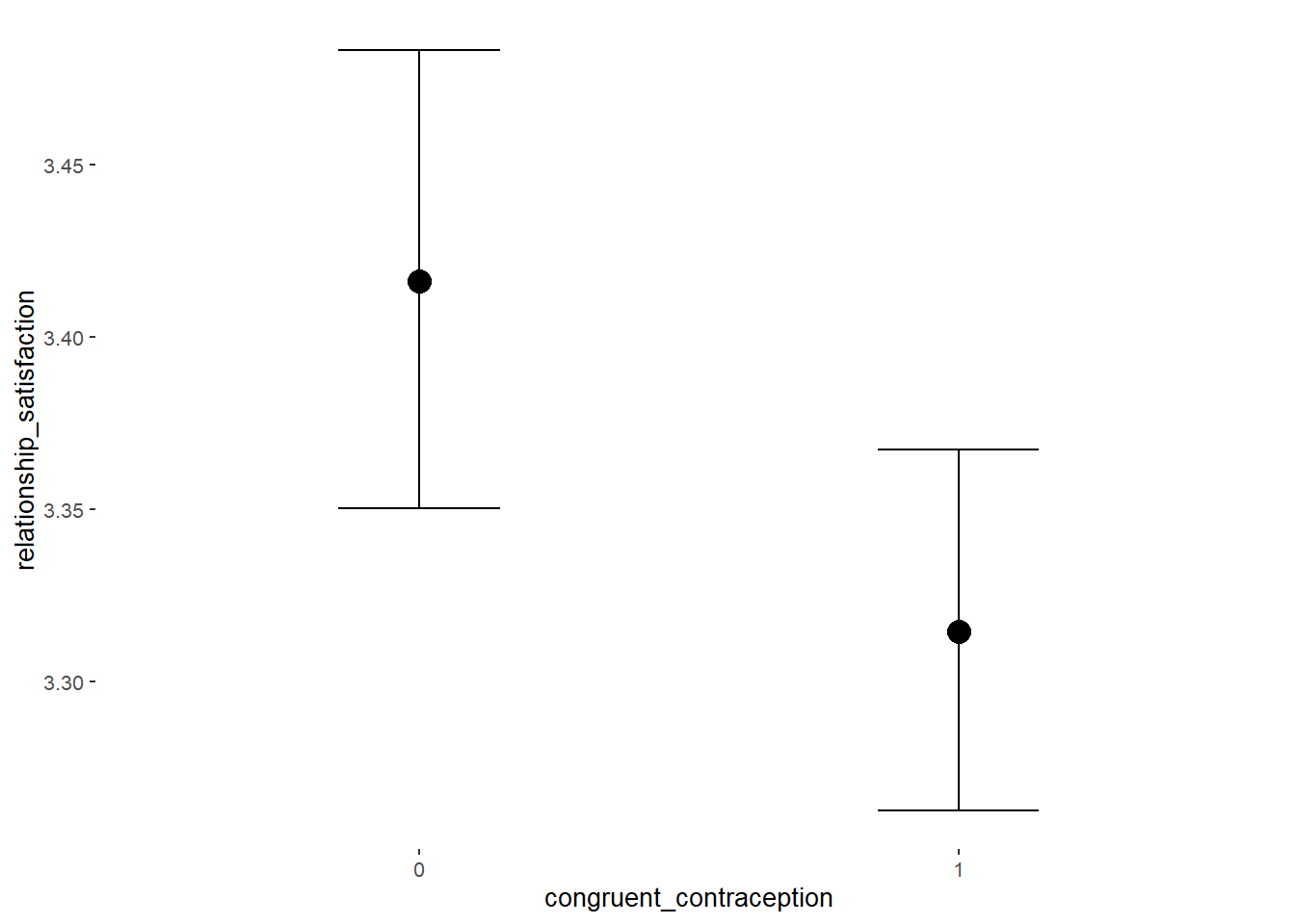
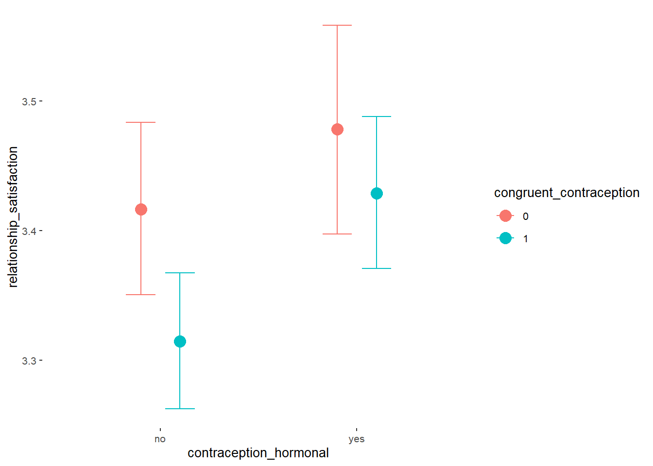
## Intercept 3.42 0.03 3.36 3.47 1.00 2468
## contraception_hormonalyes 0.06 0.05 -0.03 0.15 1.00 2218
## congruent_contraception1 -0.10 0.04 -0.17 -0.03 1.00 2157
## contraception_hormonalyes:congruent_contraception1 0.05 0.07 -0.05 0.16 1.00 2043
## Tail_ESS
## Intercept 2991
## contraception_hormonalyes 2582
## congruent_contraception1 2541
## contraception_hormonalyes:congruent_contraception1 2705
##
## Family Specific Parameters:
## Estimate Est.Error l-90% CI u-90% CI Rhat Bulk_ESS Tail_ESS
## sigma 0.42 0.01 0.40 0.44 1.00 3775 2635
##
## Draws were sampled using sampling(NUTS). For each parameter, Bulk_ESS
## and Tail_ESS are effective sample size measures, and Rhat is the potential
## scale reduction factor on split chains (at convergence, Rhat = 1).Comparison with ROPE
plot(equivalence_test(m_congruency_relsat, range = c(-0.04, 0.04), ci = 0.90,
                      parameters = "contraception"))
## Possible multicollinearity between b_contraception_hormonalyes:congruent_contraception1 and b_contraception_hormonalyes (r = 0.79). This might lead to inappropriate results. See 'Details' in '?equivalence_test'.## Picking joint bandwidth of 0.00733## Warning: Removed 1197 rows containing non-finite values (stat_density_ridges).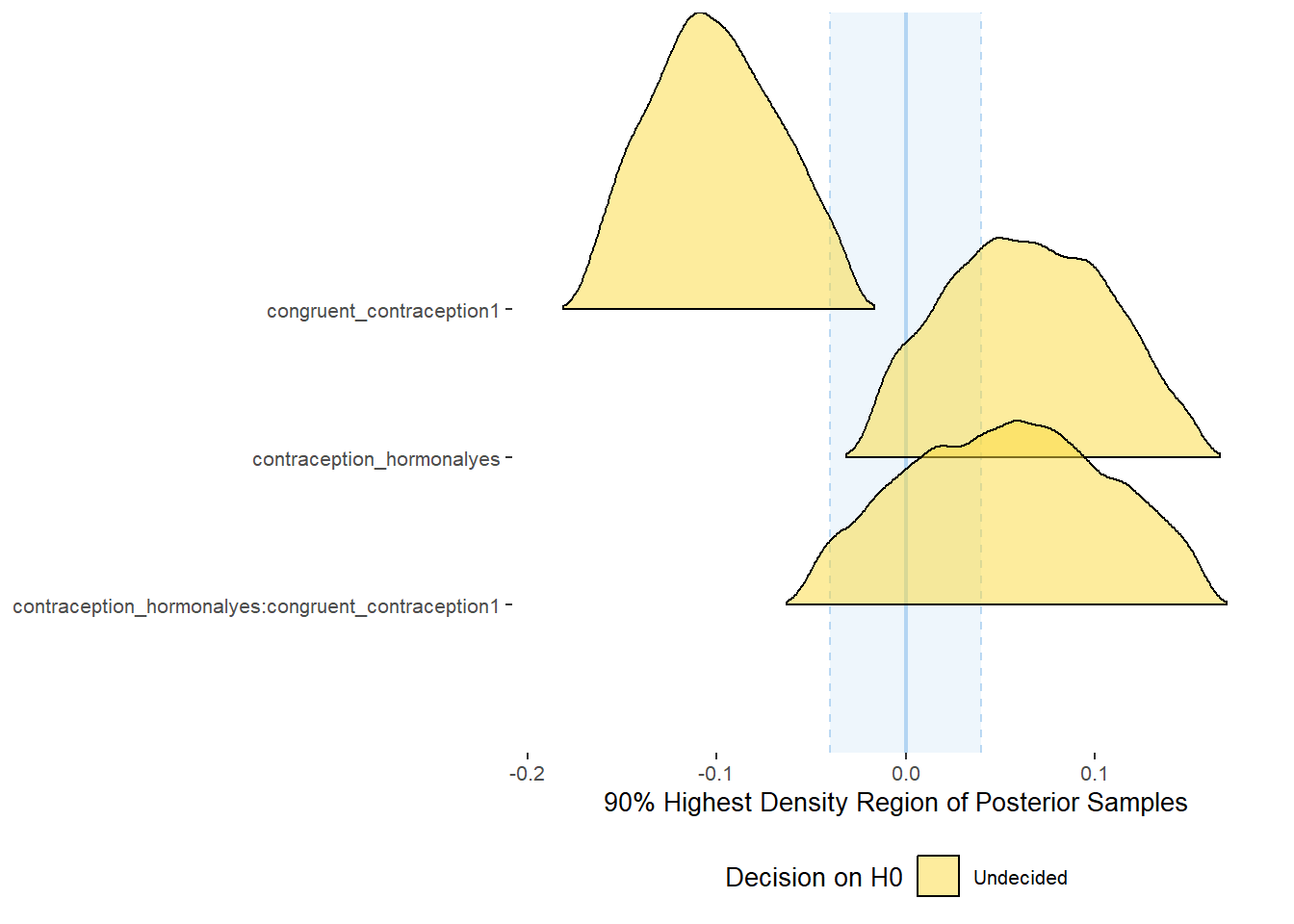
equivalence_test(m_congruency_relsat, range = c(-0.04, 0.04), ci = 0.90,
                      parameters = "contraception")
## Possible multicollinearity between b_contraception_hormonalyes:congruent_contraception1 and b_contraception_hormonalyes (r = 0.79). This might lead to inappropriate results. See 'Details' in '?equivalence_test'.## # A tibble: 3 x 10
## Parameter CI ROPE_low ROPE_high ROPE_Percentage ROPE_Equivalence HDI_low HDI_high Effects Component
## <chr> <dbl> <dbl> <dbl> <dbl> <chr> <dbl> <dbl> <chr> <chr>
## 1 b_contraceptio~ 0.9 -0.04 0.04 0.306 Undecided -0.0182 0.154 fixed conditio~
## 2 b_congruent_co~ 0.9 -0.04 0.04 0.0322 Undecided -0.168 -0.0301 fixed conditio~
## 3 b_contraceptio~ 0.9 -0.04 0.04 0.381 Undecided -0.0520 0.158 fixed conditio~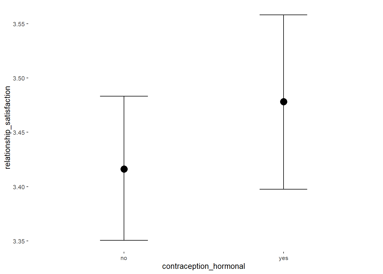
Forest Plot for Effect Sizes
m_congruency_relsat %>%
  spread_draws(b_contraception_hormonalyes, b_congruent_contraception1,
               `b_contraception_hormonalyes:congruent_contraception1`) %>%
  pivot_longer(cols = c(b_contraception_hormonalyes, b_congruent_contraception1,
               `b_contraception_hormonalyes:congruent_contraception1`),
               names_to = "condition",
               values_to = "r_condition") %>%
  mutate(condition_mean = r_condition,
         group = ifelse(condition %contains% "ontraception",
                        "Contraception", NA),
         condition = ifelse(condition == "b_contraception_hormonalyes",
                        "Hormonal Contraception",
                     ifelse(condition == "b_congruent_contraception1",
                            "Congruent Contraception",
                     ifelse(condition == "b_contraception_hormonalyes:congruent_contraception1",
                            "Interaction Hormonal Contracpetion and Congruent Contraception",
                            condition))),
         condition = factor(condition, levels = rev(c("Hormonal Contraception",
                                            "Congruent Contraception",
                                            "Interaction Hormonal Contracpetion and Congruent Contraception")))) %>%
  ggplot(aes(y = condition,
             x = condition_mean,
             fill = stat(abs(x) < 0.04))) +
  stat_halfeye() +
  geom_vline(xintercept = c(-0.04, 0.04), linetype = "dotted") +
  apatheme +
  theme(legend.position = "none") +
  scale_fill_manual(values = c("gray80", "skyblue")) +
  labs(x = "Effect Size Estimates", y = "Predictors") +
  xlim (-0.6, 0.6)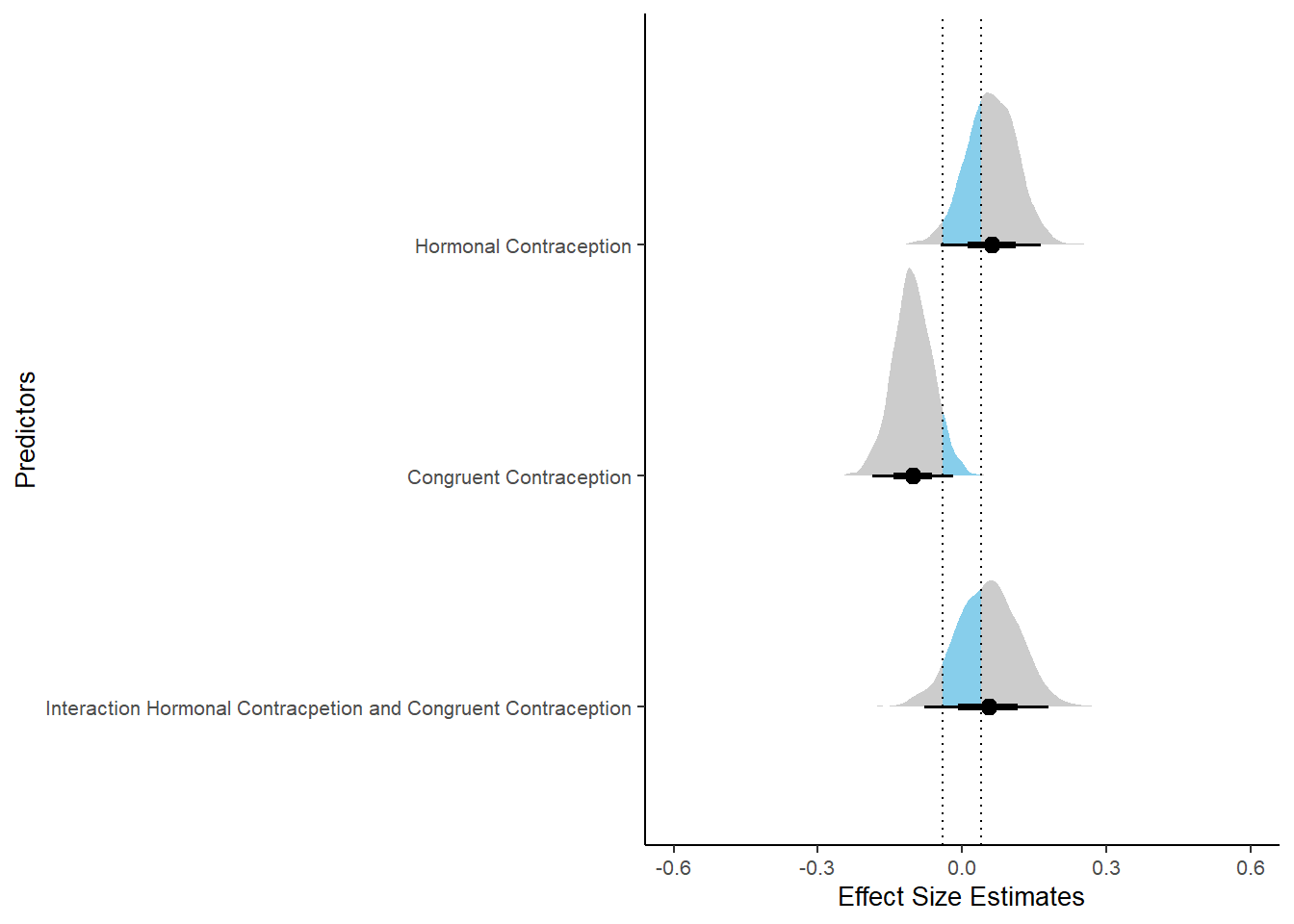
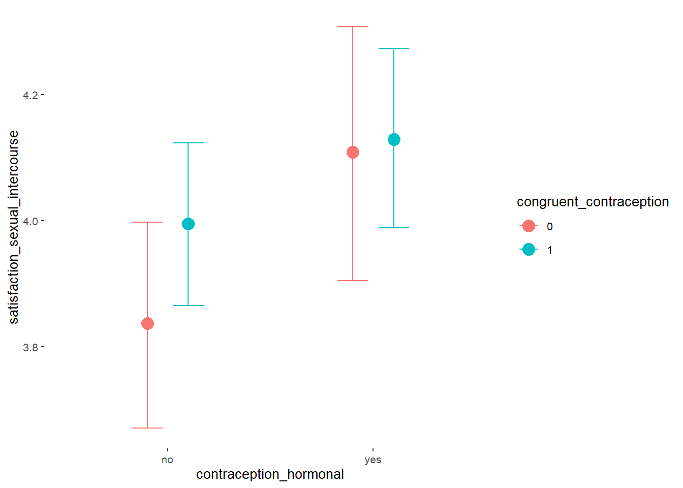
Sexual Satisfaction
Model
Summary
##  Family: gaussian
##   Links: mu = identity; sigma = identity
## Formula: satisfaction_sexual_intercourse ~ contraception_hormonal * congruent_contraception
##    Data: data (Number of observations: 710)
##   Draws: 4 chains, each with iter = 2000; warmup = 1000; thin = 1;
##          total post-warmup draws = 4000
##
## Population-Level Effects:
##                                                    Estimate Est.Error l-90% CI u-90% CI Rhat Bulk_ESS
## Intercept                                              3.84      0.08     3.70     3.97 1.00     2313
## contraception_hormonalyes                              0.27      0.13     0.05     0.49 1.00     1842
## congruent_contraception1                               0.16      0.11    -0.01     0.33 1.00     2085
## contraception_hormonalyes:congruent_contraception1    -0.14      0.16    -0.41     0.13 1.00     1756
##                                                    Tail_ESS
## Intercept                                              2741
## contraception_hormonalyes                              2335
## congruent_contraception1                               2770
## contraception_hormonalyes:congruent_contraception1     2313
##
## Family Specific Parameters:
##       Estimate Est.Error l-90% CI u-90% CI Rhat Bulk_ESS Tail_ESS
## sigma     1.04      0.03     0.99     1.08 1.00     3597     3011
##
## Draws were sampled using sampling(NUTS). For each parameter, Bulk_ESS
## and Tail_ESS are effective sample size measures, and Rhat is the potential
## scale reduction factor on split chains (at convergence, Rhat = 1).
Comparison with ROPE
plot(equivalence_test(m_congruency_sexsat, range = c(-0.11, 0.11), ci = 0.90,
                      parameters = "contraception"))
## Possible multicollinearity between b_contraception_hormonalyes:congruent_contraception1 and b_contraception_hormonalyes (r = 0.8). This might lead to inappropriate results. See 'Details' in '?equivalence_test'.## Picking joint bandwidth of 0.0183## Warning: Removed 1197 rows containing non-finite values (stat_density_ridges).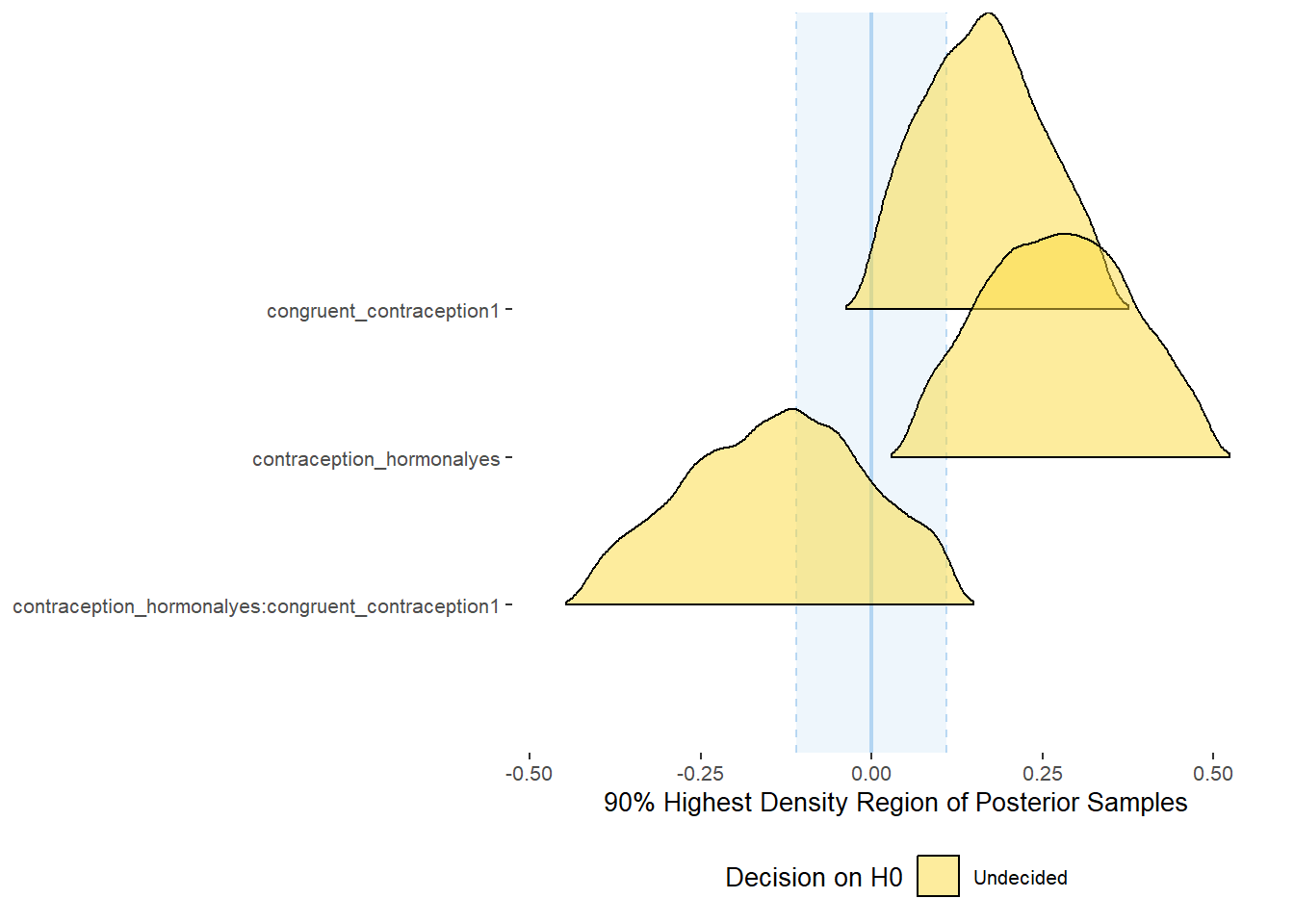
equivalence_test(m_congruency_sexsat, range = c(-0.11, 0.11), ci = 0.90,
                      parameters = "contraception")
## Possible multicollinearity between b_contraception_hormonalyes:congruent_contraception1 and b_contraception_hormonalyes (r = 0.8). This might lead to inappropriate results. See 'Details' in '?equivalence_test'.## # A tibble: 3 x 10
## Parameter CI ROPE_low ROPE_high ROPE_Percentage ROPE_Equivalence HDI_low HDI_high Effects Component
## <chr> <dbl> <dbl> <dbl> <dbl> <chr> <dbl> <dbl> <chr> <chr>
## 1 b_contracepti~ 0.9 -0.11 0.11 0.0611 Undecided 0.0601 0.492 fixed conditio~
## 2 b_congruent_c~ 0.9 -0.11 0.11 0.290 Undecided -0.00253 0.343 fixed conditio~
## 3 b_contracepti~ 0.9 -0.11 0.11 0.419 Undecided -0.419 0.119 fixed conditio~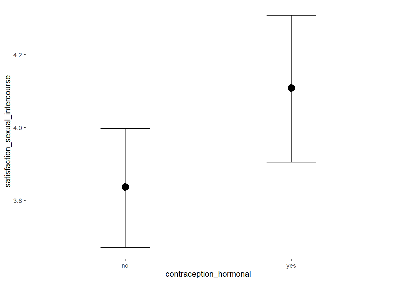
Forest Plot for Effect Sizes
m_congruency_sexsat %>%
  spread_draws(b_contraception_hormonalyes, b_congruent_contraception1,
               `b_contraception_hormonalyes:congruent_contraception1`) %>%
  pivot_longer(cols = c(b_contraception_hormonalyes, b_congruent_contraception1,
               `b_contraception_hormonalyes:congruent_contraception1`),
               names_to = "condition",
               values_to = "r_condition") %>%
  mutate(condition_mean = r_condition,
         group = ifelse(condition %contains% "ontraception",
                        "Contraception", NA),
         condition = ifelse(condition == "b_contraception_hormonalyes",
                        "Hormonal Contraception",
                     ifelse(condition == "b_congruent_contraception1",
                            "Congruent Contraception",
                     ifelse(condition == "b_contraception_hormonalyes:congruent_contraception1",
                            "Interaction Hormonal Contracpetion and Congruent Contraception",
                            condition))),
         condition = factor(condition, levels = rev(c("Hormonal Contraception",
                                            "Congruent Contraception",
                                            "Interaction Hormonal Contracpetion and Congruent Contraception")))) %>%
  ggplot(aes(y = condition,
             x = condition_mean,
             fill = stat(abs(x) < 0.11))) +
  stat_halfeye() +
  geom_vline(xintercept = c(-0.11, 0.11), linetype = "dotted") +
  apatheme +
  theme(legend.position = "none") +
  scale_fill_manual(values = c("gray80", "skyblue")) +
  labs(x = "Effect Size Estimates", y = "Predictors") +
  xlim (-0.6, 0.6)
## Warning: Removed 41 rows containing missing values (stat_slabinterval).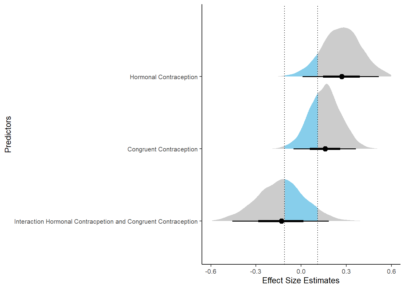
Libido
Model
Summary
##  Family: gaussian
##   Links: mu = identity; sigma = identity
## Formula: diary_libido_mean ~ contraception_hormonal * congruent_contraception
##    Data: data (Number of observations: 586)
##   Draws: 4 chains, each with iter = 2000; warmup = 1000; thin = 1;
##          total post-warmup draws = 4000
##
## Population-Level Effects:
##                                                    Estimate Est.Error l-90% CI u-90% CI Rhat Bulk_ESS
## Intercept                                              1.24      0.05     1.16     1.32 1.00     2215
## contraception_hormonalyes                             -0.03      0.08    -0.15     0.10 1.00     2021
## congruent_contraception1                               0.08      0.06    -0.02     0.18 1.00     2065
## contraception_hormonalyes:congruent_contraception1    -0.02      0.09    -0.18     0.12 1.00     1824
##                                                    Tail_ESS
## Intercept                                              2780
## contraception_hormonalyes                              2389
## congruent_contraception1                               2393
## contraception_hormonalyes:congruent_contraception1     2302
##
## Family Specific Parameters:
##       Estimate Est.Error l-90% CI u-90% CI Rhat Bulk_ESS Tail_ESS
## sigma     0.54      0.02     0.52     0.57 1.00     3484     2977
##
## Draws were sampled using sampling(NUTS). For each parameter, Bulk_ESS
## and Tail_ESS are effective sample size measures, and Rhat is the potential
## scale reduction factor on split chains (at convergence, Rhat = 1).
Comparison with ROPE
plot(equivalence_test(m_congruency_libido, range = c(-0.06, 0.06), ci = 0.90,
                      parameters = "contraception"))
## Possible multicollinearity between b_contraception_hormonalyes:congruent_contraception1 and b_contraception_hormonalyes (r = 0.79). This might lead to inappropriate results. See 'Details' in '?equivalence_test'.## Picking joint bandwidth of 0.0106## Warning: Removed 1197 rows containing non-finite values (stat_density_ridges).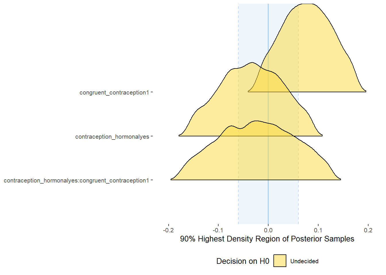
equivalence_test(m_congruency_libido, range = c(-0.06, 0.06), ci = 0.90,
                      parameters = "contraception")
## Possible multicollinearity between b_contraception_hormonalyes:congruent_contraception1 and b_contraception_hormonalyes (r = 0.79). This might lead to inappropriate results. See 'Details' in '?equivalence_test'.## # A tibble: 3 x 10
## Parameter CI ROPE_low ROPE_high ROPE_Percentage ROPE_Equivalence HDI_low HDI_high Effects Component
## <chr> <dbl> <dbl> <dbl> <dbl> <chr> <dbl> <dbl> <chr> <chr>
## 1 b_contraceptio~ 0.9 -0.06 0.06 0.585 Undecided -0.160 0.0889 fixed conditio~
## 2 b_congruent_co~ 0.9 -0.06 0.06 0.375 Undecided -0.0207 0.175 fixed conditio~
## 3 b_contraceptio~ 0.9 -0.06 0.06 0.505 Undecided -0.179 0.128 fixed conditio~
Forest Plot for Effect Sizes
m_congruency_libido %>%
  spread_draws(b_contraception_hormonalyes, b_congruent_contraception1,
               `b_contraception_hormonalyes:congruent_contraception1`) %>%
  pivot_longer(cols = c(b_contraception_hormonalyes, b_congruent_contraception1,
               `b_contraception_hormonalyes:congruent_contraception1`),
               names_to = "condition",
               values_to = "r_condition") %>%
  mutate(condition_mean = r_condition,
         group = ifelse(condition %contains% "ontraception",
                        "Contraception", NA),
         condition = ifelse(condition == "b_contraception_hormonalyes",
                        "Hormonal Contraception",
                     ifelse(condition == "b_congruent_contraception1",
                            "Congruent Contraception",
                     ifelse(condition == "b_contraception_hormonalyes:congruent_contraception1",
                            "Interaction Hormonal Contracpetion and Congruent Contraception",
                            condition))),
         condition = factor(condition, levels = rev(c("Hormonal Contraception",
                                            "Congruent Contraception",
                                            "Interaction Hormonal Contracpetion and Congruent Contraception")))) %>%
  ggplot(aes(y = condition,
             x = condition_mean,
             fill = stat(abs(x) < 0.06))) +
  stat_halfeye() +
  geom_vline(xintercept = c(-0.06, 0.06), linetype = "dotted") +
  apatheme +
  theme(legend.position = "none") +
  scale_fill_manual(values = c("gray80", "skyblue")) +
  labs(x = "Effect Size Estimates", y = "Predictors") +
  xlim (-0.6, 0.6)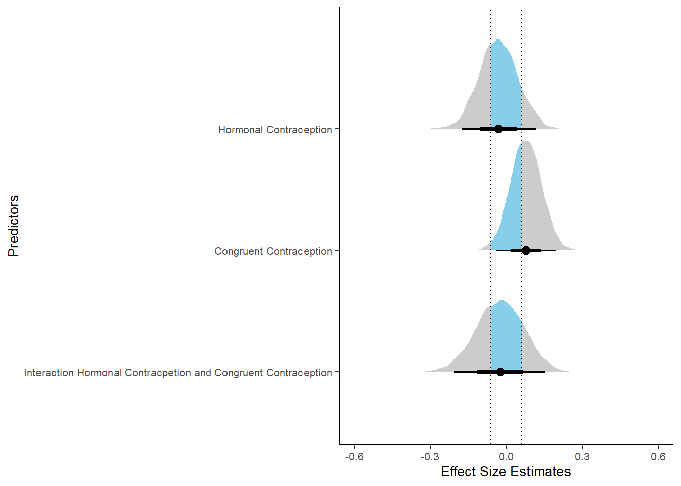
Sexual Frequency (Penetrative Intercourse)
Model
Summary
##  Family: poisson
##   Links: mu = log
## Formula: diary_sex_active_sex_sum ~ offset(log(number_of_days)) + contraception_hormonal * congruent_contraception
##    Data: data (Number of observations: 576)
##   Draws: 4 chains, each with iter = 2000; warmup = 1000; thin = 1;
##          total post-warmup draws = 4000
##
## Population-Level Effects:
##                                                    Estimate Est.Error l-90% CI u-90% CI Rhat Bulk_ESS
## Intercept                                             -1.87      0.03    -1.92    -1.82 1.00     1711
## contraception_hormonalyes                              0.14      0.05     0.06     0.22 1.00     1579
## congruent_contraception1                               0.09      0.04     0.02     0.15 1.00     1787
## contraception_hormonalyes:congruent_contraception1    -0.05      0.06    -0.15     0.05 1.00     1542
##                                                    Tail_ESS
## Intercept                                              2547
## contraception_hormonalyes                              2111
## congruent_contraception1                               2485
## contraception_hormonalyes:congruent_contraception1     2150
##
## Draws were sampled using sampling(NUTS). For each parameter, Bulk_ESS
## and Tail_ESS are effective sample size measures, and Rhat is the potential
## scale reduction factor on split chains (at convergence, Rhat = 1).
Comparison with ROPE
plot(equivalence_test(m_congruency_sexfreqpen, range = c(-0.05, 0.05), ci = 0.90,
                      parameters = "contraception"))
## Possible multicollinearity between b_contraception_hormonalyes:congruent_contraception1 and b_contraception_hormonalyes (r = 0.82). This might lead to inappropriate results. See 'Details' in '?equivalence_test'.## Picking joint bandwidth of 0.00692## Warning: Removed 1197 rows containing non-finite values (stat_density_ridges).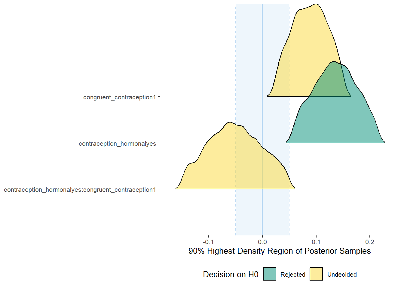
equivalence_test(m_congruency_sexfreqpen, range = c(-0.05, 0.05), ci = 0.90,
                      parameters = "contraception")
## Possible multicollinearity between b_contraception_hormonalyes:congruent_contraception1 and b_contraception_hormonalyes (r = 0.82). This might lead to inappropriate results. See 'Details' in '?equivalence_test'.## # A tibble: 3 x 10
## Parameter CI ROPE_low ROPE_high ROPE_Percentage ROPE_Equivalence HDI_low HDI_high Effects Component
## <chr> <dbl> <dbl> <dbl> <dbl> <chr> <dbl> <dbl> <chr> <chr>
## 1 b_contraceptio~ 0.9 -0.05 0.05 0 Rejected 0.0562 0.215 fixed conditio~
## 2 b_congruent_co~ 0.9 -0.05 0.05 0.135 Undecided 0.0224 0.152 fixed conditio~
## 3 b_contraceptio~ 0.9 -0.05 0.05 0.483 Undecided -0.150 0.0494 fixed conditio~Plots
conditional_effects(m_congruency_sexfreqpen,
                    effects = "contraception_hormonal:congruent_contraception",
                    conditions = data.frame(number_of_days = 1))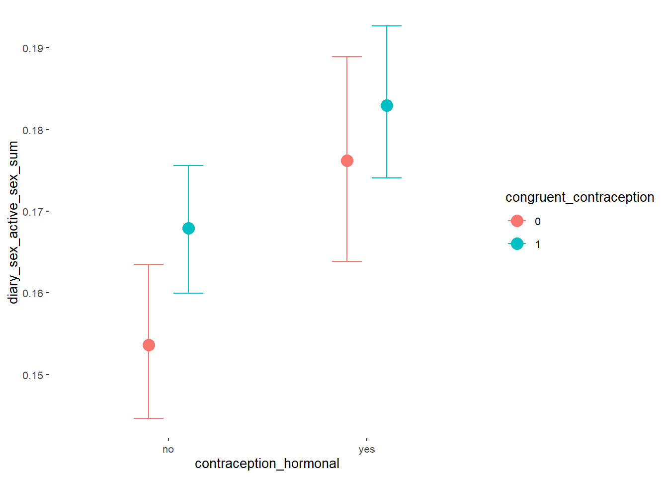
Forest Plot for Effect Sizes
m_congruency_sexfreqpen %>%
  spread_draws(b_contraception_hormonalyes, b_congruent_contraception1,
               `b_contraception_hormonalyes:congruent_contraception1`) %>%
  pivot_longer(cols = c(b_contraception_hormonalyes, b_congruent_contraception1,
               `b_contraception_hormonalyes:congruent_contraception1`),
               names_to = "condition",
               values_to = "r_condition") %>%
  mutate(condition_mean = r_condition,
         group = ifelse(condition %contains% "ontraception",
                        "Contraception", NA),
         condition = ifelse(condition == "b_contraception_hormonalyes",
                        "Hormonal Contraception",
                     ifelse(condition == "b_congruent_contraception1",
                            "Congruent Contraception",
                     ifelse(condition == "b_contraception_hormonalyes:congruent_contraception1",
                            "Interaction Hormonal Contracpetion and Congruent Contraception",
                            condition))),
         condition = factor(condition, levels = rev(c("Hormonal Contraception",
                                            "Congruent Contraception",
                                            "Interaction Hormonal Contracpetion and Congruent Contraception")))) %>%
  ggplot(aes(y = condition,
             x = condition_mean,
             fill = stat(abs(x) < 0.05))) +
  stat_halfeye() +
  geom_vline(xintercept = c(-0.05, 0.051), linetype = "dotted") +
  apatheme +
  theme(legend.position = "none") +
  scale_fill_manual(values = c("gray80", "skyblue")) +
  labs(x = "Effect Size Estimates", y = "Predictors")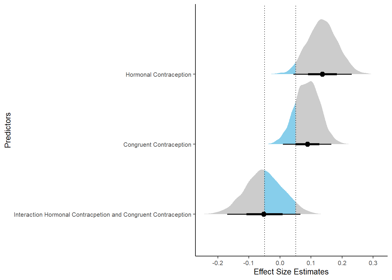
Masturbation Frequency
Model
Summary
##  Family: poisson
##   Links: mu = log
## Formula: diary_masturbation_sum ~ offset(log(number_of_days)) + contraception_hormonal * congruent_contraception
##    Data: data (Number of observations: 576)
##   Draws: 4 chains, each with iter = 2000; warmup = 1000; thin = 1;
##          total post-warmup draws = 4000
##
## Population-Level Effects:
##                                                    Estimate Est.Error l-90% CI u-90% CI Rhat Bulk_ESS
## Intercept                                             -2.09      0.03    -2.14    -2.03 1.01     2047
## contraception_hormonalyes                             -0.41      0.06    -0.51    -0.31 1.01     1674
## congruent_contraception1                               0.11      0.04     0.04     0.18 1.01     1793
## contraception_hormonalyes:congruent_contraception1     0.03      0.07    -0.09     0.16 1.00     1599
##                                                    Tail_ESS
## Intercept                                              2746
## contraception_hormonalyes                              2131
## congruent_contraception1                               2070
## contraception_hormonalyes:congruent_contraception1     2354
##
## Draws were sampled using sampling(NUTS). For each parameter, Bulk_ESS
## and Tail_ESS are effective sample size measures, and Rhat is the potential
## scale reduction factor on split chains (at convergence, Rhat = 1).
Comparison with ROPE
plot(equivalence_test(m_congruency_masfreq, range = c(-0.05, 0.05), ci = 0.90,
                      parameters = "contraception"))
## Possible multicollinearity between b_contraception_hormonalyes:congruent_contraception1 and b_contraception_hormonalyes (r = 0.82). This might lead to inappropriate results. See 'Details' in '?equivalence_test'.## Picking joint bandwidth of 0.00834## Warning: Removed 1197 rows containing non-finite values (stat_density_ridges).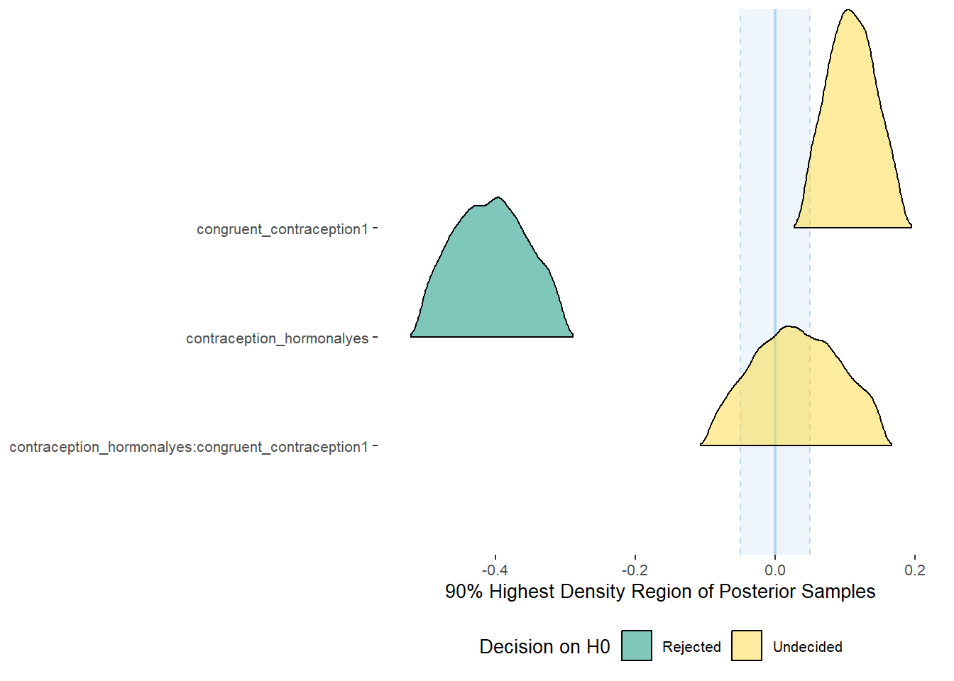
equivalence_test(m_congruency_masfreq, range = c(-0.05, 0.05), ci = 0.90,
                      parameters = "contraception")
## Possible multicollinearity between b_contraception_hormonalyes:congruent_contraception1 and b_contraception_hormonalyes (r = 0.82). This might lead to inappropriate results. See 'Details' in '?equivalence_test'.## # A tibble: 3 x 10
## Parameter CI ROPE_low ROPE_high ROPE_Percentage ROPE_Equivalence HDI_low HDI_high Effects Component
## <chr> <dbl> <dbl> <dbl> <dbl> <chr> <dbl> <dbl> <chr> <chr>
## 1 b_contraceptio~ 0.9 -0.05 0.05 0 Rejected -0.506 -0.302 fixed conditio~
## 2 b_congruent_co~ 0.9 -0.05 0.05 0.0294 Undecided 0.0426 0.180 fixed conditio~
## 3 b_contraceptio~ 0.9 -0.05 0.05 0.510 Undecided -0.0927 0.153 fixed conditio~Plots
conditional_effects(m_congruency_masfreq,
                    effects = "contraception_hormonal:congruent_contraception",
                    conditions = data.frame(number_of_days = 1))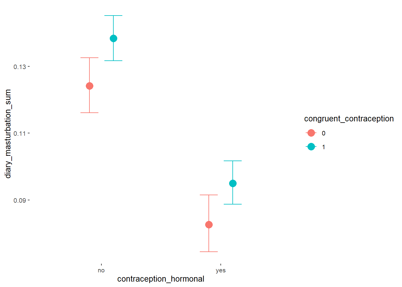
Forest Plot for Effect Sizes
m_congruency_masfreq %>%
spread_draws(b_contraception_hormonalyes, b_congruent_contraception1,
               `b_contraception_hormonalyes:congruent_contraception1`) %>%
  pivot_longer(cols = c(b_contraception_hormonalyes, b_congruent_contraception1,
               `b_contraception_hormonalyes:congruent_contraception1`),
               names_to = "condition",
               values_to = "r_condition") %>%
  mutate(condition_mean = r_condition,
         group = ifelse(condition %contains% "ontraception",
                        "Contraception", NA),
         condition = ifelse(condition == "b_contraception_hormonalyes",
                        "Hormonal Contraception",
                     ifelse(condition == "b_congruent_contraception1",
                            "Congruent Contraception",
                     ifelse(condition == "b_contraception_hormonalyes:congruent_contraception1",
                            "Interaction Hormonal Contracpetion and Congruent Contraception",
                            condition))),
         condition = factor(condition, levels = rev(c("Hormonal Contraception",
                                            "Congruent Contraception",
                                            "Interaction Hormonal Contracpetion and Congruent Contraception")))) %>%
  ggplot(aes(y = condition,
             x = condition_mean,
             fill = stat(abs(x) < 0.05))) +
  stat_halfeye() +
  geom_vline(xintercept = c(-0.05, 0.05), linetype = "dotted") +
  apatheme +
  theme(legend.position = "none") +
  scale_fill_manual(values = c("gray80", "skyblue")) +
  labs(x = "Effect Size Estimates", y = "Predictors")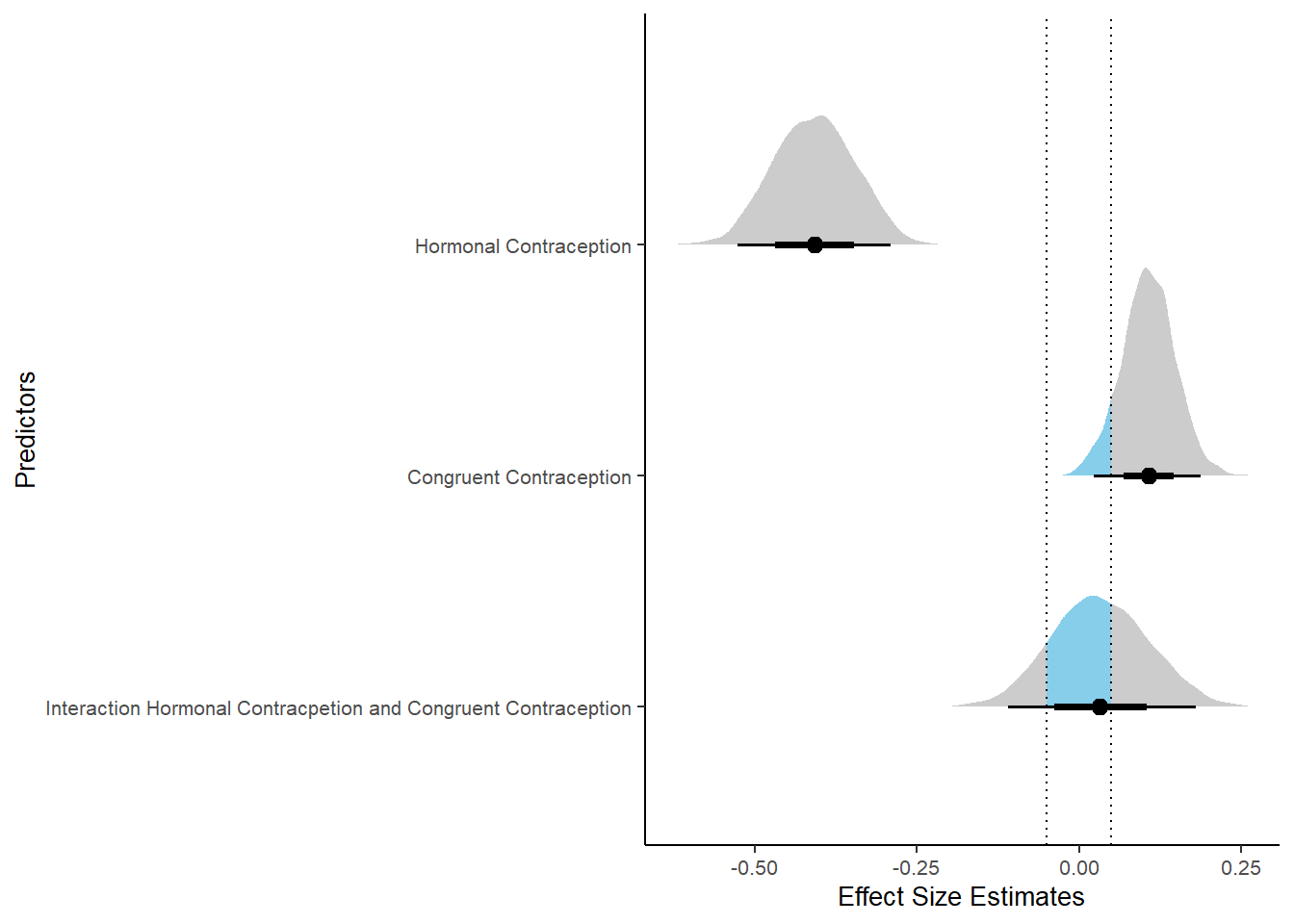
Controlled Models: Effects of (In)Congruenct HC Use
Attractiveness of Partner
Model
m_congruency_atrr_controlled = brm(attractiveness_partner ~
                          contraception_hormonal * congruent_contraception +
                             age + net_income + relationship_duration_factor +
                              education_years +
                              bfi_extra + bfi_neuro + bfi_agree + bfi_consc + bfi_open +
                              religiosity,
                data = data, family = gaussian(),
                file = "m_congruency_atrr_controlled_robust")
Summary
## Warning: Parts of the model have not converged (some Rhats are > 1.05). Be careful when analysing the results!
## We recommend running more iterations and/or setting stronger priors.
## Family: gaussian
## Links: mu = identity; sigma = identity
## Formula: attractiveness_partner ~ contraception_hormonal * congruent_contraception + age + net_income + relationship_duration_factor + education_years + bfi_extra + bfi_neuro + bfi_agree + bfi_consc + bfi_open + religiosity
## Data: data (Number of observations: 710)
## Draws: 4 chains, each with iter = 2000; warmup = 1000; thin = 1;
## total post-warmup draws = 4000
##
## Population-Level Effects:
## Estimate Est.Error l-90% CI u-90% CI Rhat Bulk_ESS
## Intercept 63.96 307.30 -545.89 528.00 2.43 5
## contraception_hormonalyes 0.10 0.11 -0.06 0.29 1.33 10
## congruent_contraception1 0.08 0.08 -0.04 0.22 1.22 14
## age -0.00 0.01 -0.01 0.01 1.09 34
## net_incomeeuro_500_1000 -0.00 0.05 -0.09 0.09 1.15 22
## net_incomeeuro_1000_2000 0.10 0.08 -0.03 0.21 1.08 42
## net_incomeeuro_2000_3000 0.10 0.11 -0.08 0.27 1.05 42
## net_incomeeuro_gt_3000 0.03 0.21 -0.30 0.37 1.07 46
## net_incomedont_tell 0.00 0.19 -0.28 0.31 1.10 31
## relationship_duration_factorPartnered_upto12months -60.50 307.37 -524.70 549.69 2.43 5
## relationship_duration_factorPartnered_upto28months -60.39 307.37 -524.58 549.79 2.43 5
## relationship_duration_factorPartnered_upto52months -60.53 307.37 -524.72 549.69 2.43 5
## relationship_duration_factorPartnered_morethan52months -60.58 307.37 -524.78 549.47 2.43 5
## education_years 0.01 0.01 -0.01 0.02 1.15 20
## bfi_extra 0.03 0.04 -0.03 0.09 1.13 33
## bfi_neuro -0.01 0.04 -0.08 0.06 1.09 33
## bfi_agree 0.08 0.05 -0.00 0.16 1.13 21
## bfi_consc 0.02 0.05 -0.06 0.11 1.27 12
## bfi_open 0.06 0.04 -0.01 0.13 1.17 17
## religiosity 0.00 0.02 -0.03 0.03 1.24 13
## contraception_hormonalyes:congruent_contraception1 -0.02 0.13 -0.25 0.18 1.31 11
## Tail_ESS
## Intercept NA
## contraception_hormonalyes NA
## congruent_contraception1 NA
## age NA
## net_incomeeuro_500_1000 NA
## net_incomeeuro_1000_2000 NA
## net_incomeeuro_2000_3000 NA
## net_incomeeuro_gt_3000 NA
## net_incomedont_tell NA
## relationship_duration_factorPartnered_upto12months NA
## relationship_duration_factorPartnered_upto28months NA
## relationship_duration_factorPartnered_upto52months NA
## relationship_duration_factorPartnered_morethan52months NA
## education_years NA
## bfi_extra NA
## bfi_neuro NA
## bfi_agree NA
## bfi_consc NA
## bfi_open NA
## religiosity NA
## contraception_hormonalyes:congruent_contraception1 NA
##
## Family Specific Parameters:
## Estimate Est.Error l-90% CI u-90% CI Rhat Bulk_ESS Tail_ESS
## sigma 0.72 0.02 0.70 0.76 1.24 15 NA
##
## Draws were sampled using sampling(NUTS). For each parameter, Bulk_ESS
## and Tail_ESS are effective sample size measures, and Rhat is the potential
## scale reduction factor on split chains (at convergence, Rhat = 1).Comparison with ROPE
plot(equivalence_test(m_congruency_atrr_controlled, range = c(-0.07, 0.07), ci = 0.90,
                      parameters = "contraception"))
## Possible multicollinearity between b_contraception_hormonalyes:congruent_contraception1 and b_contraception_hormonalyes (r = 0.81), b_contraception_hormonalyes:congruent_contraception1 and b_congruent_contraception1 (r = 0.71). This might lead to inappropriate results. See 'Details' in '?equivalence_test'.## Picking joint bandwidth of 0.0148## Warning: Removed 1197 rows containing non-finite values (stat_density_ridges).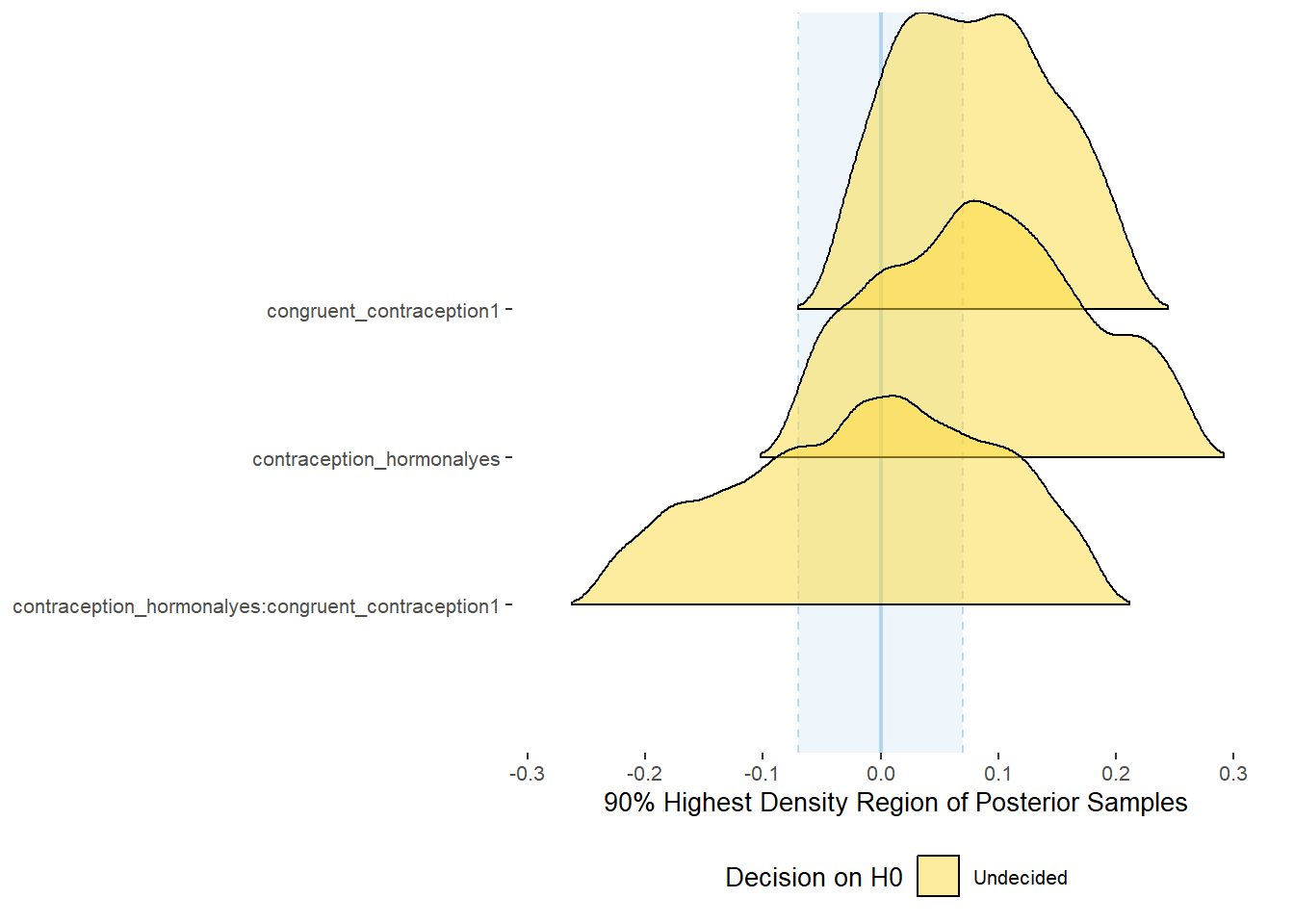
equivalence_test(m_congruency_atrr_controlled, range = c(-0.07, 0.07), ci = 0.90,
                      parameters = "contraception")
## Possible multicollinearity between b_contraception_hormonalyes:congruent_contraception1 and b_contraception_hormonalyes (r = 0.81), b_contraception_hormonalyes:congruent_contraception1 and b_congruent_contraception1 (r = 0.71). This might lead to inappropriate results. See 'Details' in '?equivalence_test'.## # A tibble: 3 x 10
## Parameter CI ROPE_low ROPE_high ROPE_Percentage ROPE_Equivalence HDI_low HDI_high Effects Component
## <chr> <dbl> <dbl> <dbl> <dbl> <chr> <dbl> <dbl> <chr> <chr>
## 1 b_contraceptio~ 0.9 -0.07 0.07 0.427 Undecided -0.0769 0.266 fixed conditio~
## 2 b_congruent_co~ 0.9 -0.07 0.07 0.460 Undecided -0.0417 0.218 fixed conditio~
## 3 b_contraceptio~ 0.9 -0.07 0.07 0.447 Undecided -0.239 0.187 fixed conditio~


Forest Plot for Effect Sizes
m_congruency_atrr_controlled %>%
  spread_draws(b_contraception_hormonalyes, b_congruent_contraception1,
               `b_contraception_hormonalyes:congruent_contraception1`,
               b_age,
               b_net_incomeeuro_500_1000, b_net_incomeeuro_1000_2000,
               b_net_incomeeuro_2000_3000, b_net_incomeeuro_gt_3000, b_net_incomedont_tell,
               b_relationship_duration_factorPartnered_upto28months,
               b_relationship_duration_factorPartnered_upto52months,
               b_relationship_duration_factorPartnered_morethan52months,
               b_education_years,
               b_bfi_extra, b_bfi_neuro, b_bfi_agree, b_bfi_consc, b_bfi_open,
               b_religiosity) %>%
  pivot_longer(cols = c(b_contraception_hormonalyes, b_congruent_contraception1,
               `b_contraception_hormonalyes:congruent_contraception1`,
                        b_age,
               b_net_incomeeuro_500_1000, b_net_incomeeuro_1000_2000,
               b_net_incomeeuro_2000_3000, b_net_incomeeuro_gt_3000, b_net_incomedont_tell,
               b_relationship_duration_factorPartnered_upto28months,
               b_relationship_duration_factorPartnered_upto52months,
               b_relationship_duration_factorPartnered_morethan52months,
               b_education_years,
               b_bfi_extra, b_bfi_neuro, b_bfi_agree, b_bfi_consc, b_bfi_open,
               b_religiosity),
               names_to = "condition",
               values_to = "r_condition") %>%
  mutate(condition_mean = r_condition,
         group = ifelse(condition %contains% "b_relationship_duration_factor",
                        "Relationship Duration",
                        ifelse(condition %contains% "b_net_income",
                               "Income",
                               NA)),
         group = ifelse(condition %contains% "ontraception",
                        "Contraception", group),
         condition = ifelse(condition == "b_contraception_hormonalyes",
                        "Hormonal Contraception",
                     ifelse(condition == "b_congruent_contraception1",
                            "Congruent Contraception",
                     ifelse(condition == "b_contraception_hormonalyes:congruent_contraception1",
                            "Interaction Hormonal Contracpetion and Congruent Contraception",
                            condition))),
         condition = ifelse(condition == "b_age", "Age",
                ifelse(condition == "b_net_incomeeuro_500_1000", "500-1000 Euro",
                ifelse(condition == "b_net_incomeeuro_1000_2000", "1000-2000 Euro",
                ifelse(condition == "b_net_incomeeuro_2000_3000", "2000-3000 Euro",
                ifelse(condition == "b_net_incomeeuro_gt_3000", ">3000 Euro",
                ifelse(condition == "b_net_incomedont_tell", "do not tell",
                ifelse(condition == "b_relationship_duration_factorPartnered_upto28months",
                       "13-28 months",
                ifelse(condition == "b_relationship_duration_factorPartnered_upto52months",
                       "29-52 months",
                ifelse(condition == "b_relationship_duration_factorPartnered_morethan52months",
                       ">52 months",
                ifelse(condition == "b_education_years", "Years of Education",
                ifelse(condition == "b_bfi_extra", "Extraversion",
                ifelse(condition == "b_bfi_neuro", "Neuroticism",
                ifelse(condition == "b_bfi_agree", "Agreeableness",
                ifelse(condition == "b_bfi_consc", "Conscientiousness",
                ifelse(condition == "b_bfi_open", "Openness",
                ifelse(condition == "b_religiosity", "Religiosity",
                       condition)))))))))))))))),
         group = ifelse(is.na(group), condition, group),
         condition = factor(condition, levels = rev(c("Hormonal Contraception",
                                        "Congruent Contraception",
                                        "Interaction Hormonal Contracpetion and Congruent Contraception",
                                        "Age",
                                        "500-1000 Euro", "1000-2000 Euro",
                                        "2000-3000 Euro", ">3000 Euro", "do not tell",
                                        "13-28 months", "29-52 months",
                                        ">52 months",
                                        "Years of Education",
                                        "Extraversion", "Neuroticism", "Agreeableness",
                                         "Conscientiousness","Openness","Religiosity"))),
         group = factor(group, levels = c("Contraception", "Age", "Income",
                                          "Relationship Duration","Years of Education",
                                          "Extraversion", "Neuroticism", "Agreeableness",
                                         "Conscientiousness","Openness","Religiosity"))) %>%
  ggplot(aes(y = condition,
             x = condition_mean,
             fill = stat(abs(x) < 0.07))) +
  stat_halfeye() +
  geom_vline(xintercept = c(-0.07, 0.07), linetype = "dotted") +
  apatheme +
  theme(legend.position = "none") +
  scale_fill_manual(values = c("gray80", "skyblue")) +
  labs(x = "Effect Size Estimates", y = "Predictors")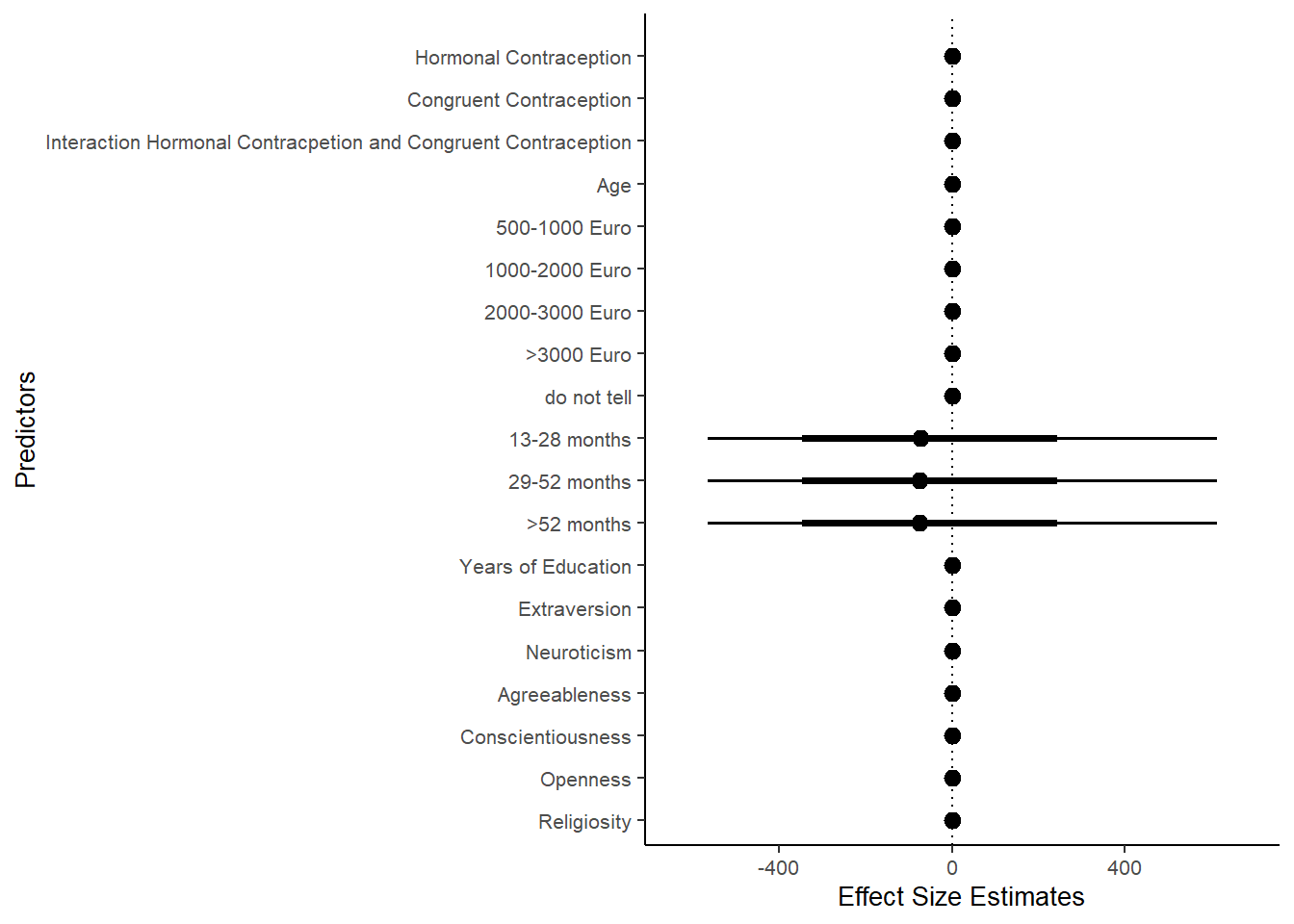
Relationship Satisfaction
Model
m_congruency_relsat_controlled = brm(relationship_satisfaction ~
                          contraception_hormonal * congruent_contraception +
                             age + net_income + relationship_duration_factor +
                              education_years +
                              bfi_extra + bfi_neuro + bfi_agree + bfi_consc + bfi_open +
                              religiosity,
                data = data, family = gaussian(),
                file = "m_congruency_relsat_controlled_robust")
Summary
## Warning: Parts of the model have not converged (some Rhats are > 1.05). Be careful when analysing the results!
## We recommend running more iterations and/or setting stronger priors.
## Family: gaussian
## Links: mu = identity; sigma = identity
## Formula: relationship_satisfaction ~ contraception_hormonal * congruent_contraception + age + net_income + relationship_duration_factor + education_years + bfi_extra + bfi_neuro + bfi_agree + bfi_consc + bfi_open + religiosity
## Data: data (Number of observations: 710)
## Draws: 4 chains, each with iter = 2000; warmup = 1000; thin = 1;
## total post-warmup draws = 4000
##
## Population-Level Effects:
## Estimate Est.Error l-90% CI u-90% CI Rhat Bulk_ESS
## Intercept 203.22 279.83 -156.84 609.50 2.65 5
## contraception_hormonalyes 0.04 0.07 -0.07 0.14 1.35 10
## congruent_contraception1 -0.07 0.05 -0.15 0.01 1.43 8
## age -0.00 0.00 -0.01 0.00 1.16 17
## net_incomeeuro_500_1000 0.06 0.04 -0.01 0.12 1.36 10
## net_incomeeuro_1000_2000 0.00 0.05 -0.08 0.09 1.20 18
## net_incomeeuro_2000_3000 0.03 0.08 -0.10 0.15 1.52 8
## net_incomeeuro_gt_3000 0.09 0.14 -0.15 0.33 1.17 17
## net_incomedont_tell -0.06 0.09 -0.21 0.10 1.24 14
## relationship_duration_factorPartnered_upto12months -199.82 279.77 -605.95 160.08 2.65 5
## relationship_duration_factorPartnered_upto28months -199.62 279.77 -605.76 160.29 2.65 5
## relationship_duration_factorPartnered_upto52months -199.68 279.77 -605.83 160.25 2.65 5
## relationship_duration_factorPartnered_morethan52months -199.68 279.77 -605.83 160.18 2.65 5
## education_years -0.00 0.00 -0.01 0.00 1.08 40
## bfi_extra 0.02 0.02 -0.01 0.05 1.09 44
## bfi_neuro 0.02 0.02 -0.02 0.06 1.16 19
## bfi_agree -0.03 0.02 -0.07 0.01 1.06 54
## bfi_consc 0.00 0.03 -0.05 0.04 1.32 10
## bfi_open -0.02 0.03 -0.07 0.03 1.19 19
## religiosity 0.03 0.01 0.01 0.05 1.08 38
## contraception_hormonalyes:congruent_contraception1 0.05 0.08 -0.08 0.18 1.53 7
## Tail_ESS
## Intercept NA
## contraception_hormonalyes NA
## congruent_contraception1 NA
## age NA
## net_incomeeuro_500_1000 NA
## net_incomeeuro_1000_2000 NA
## net_incomeeuro_2000_3000 NA
## net_incomeeuro_gt_3000 NA
## net_incomedont_tell NA
## relationship_duration_factorPartnered_upto12months NA
## relationship_duration_factorPartnered_upto28months NA
## relationship_duration_factorPartnered_upto52months NA
## relationship_duration_factorPartnered_morethan52months NA
## education_years NA
## bfi_extra NA
## bfi_neuro NA
## bfi_agree NA
## bfi_consc NA
## bfi_open NA
## religiosity NA
## contraception_hormonalyes:congruent_contraception1 NA
##
## Family Specific Parameters:
## Estimate Est.Error l-90% CI u-90% CI Rhat Bulk_ESS Tail_ESS
## sigma 0.41 0.01 0.40 0.43 1.22 15 NA
##
## Draws were sampled using sampling(NUTS). For each parameter, Bulk_ESS
## and Tail_ESS are effective sample size measures, and Rhat is the potential
## scale reduction factor on split chains (at convergence, Rhat = 1).Comparison with ROPE
plot(equivalence_test(m_congruency_relsat_controlled, range = c(-0.04, 0.04), ci = 0.90,
                      parameters = "contraception"))
## Possible multicollinearity between b_contraception_hormonalyes:congruent_contraception1 and b_contraception_hormonalyes (r = 0.84), b_contraception_hormonalyes:congruent_contraception1 and b_congruent_contraception1 (r = 0.72). This might lead to inappropriate results. See 'Details' in '?equivalence_test'.## Picking joint bandwidth of 0.00938## Warning: Removed 1197 rows containing non-finite values (stat_density_ridges).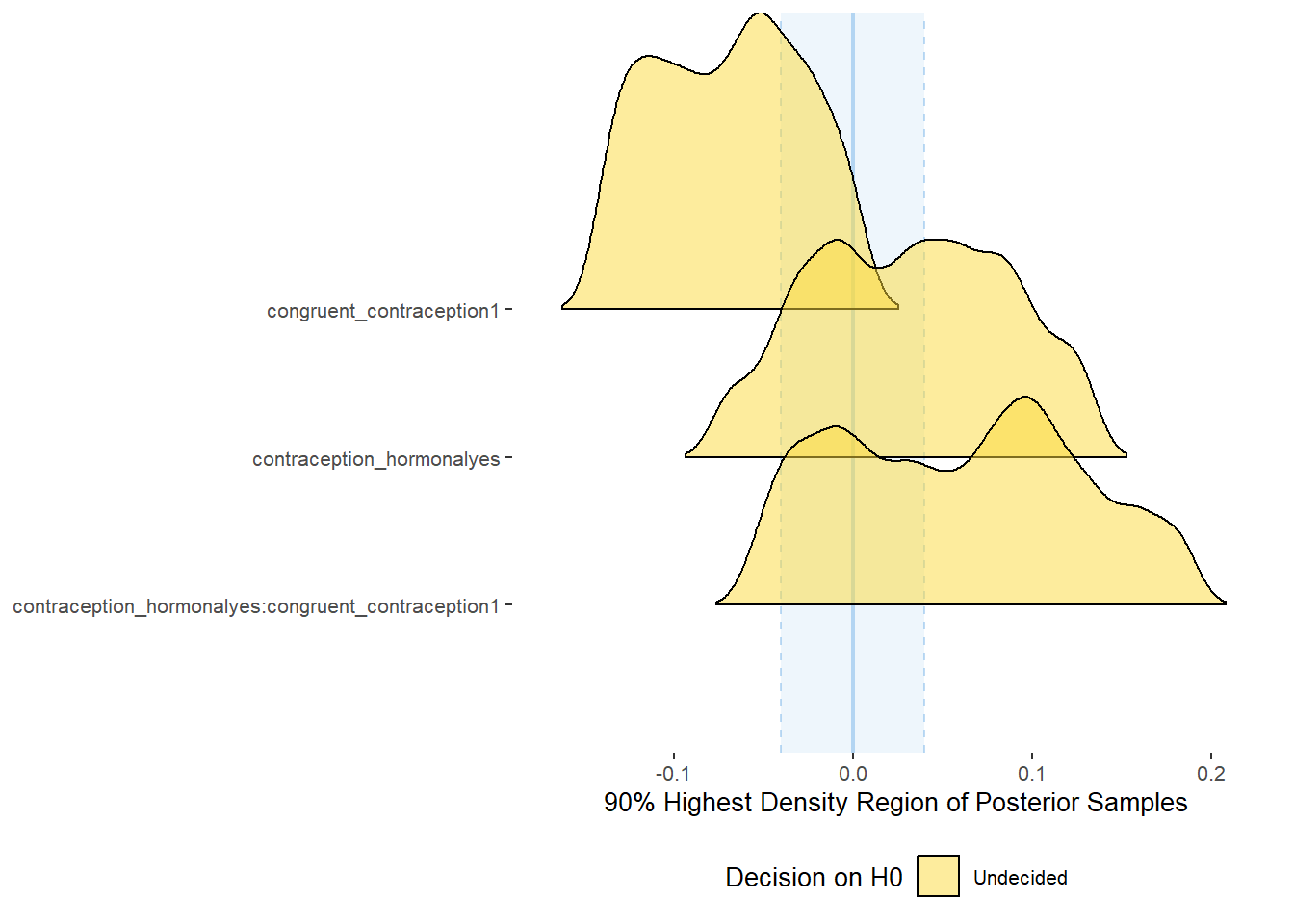
equivalence_test(m_congruency_relsat_controlled, range = c(-0.04, 0.04), ci = 0.90,
                      parameters = "contraception")
## Possible multicollinearity between b_contraception_hormonalyes:congruent_contraception1 and b_contraception_hormonalyes (r = 0.84), b_contraception_hormonalyes:congruent_contraception1 and b_congruent_contraception1 (r = 0.72). This might lead to inappropriate results. See 'Details' in '?equivalence_test'.## # A tibble: 3 x 10
## Parameter CI ROPE_low ROPE_high ROPE_Percentage ROPE_Equivalence HDI_low HDI_high Effects Component
## <chr> <dbl> <dbl> <dbl> <dbl> <chr> <dbl> <dbl> <chr> <chr>
## 1 b_contraceptio~ 0.9 -0.04 0.04 0.450 Undecided -0.0768 0.135 fixed conditio~
## 2 b_congruent_co~ 0.9 -0.04 0.04 0.277 Undecided -0.143 0.00709 fixed conditio~
## 3 b_contraceptio~ 0.9 -0.04 0.04 0.359 Undecided -0.0599 0.191 fixed conditio~
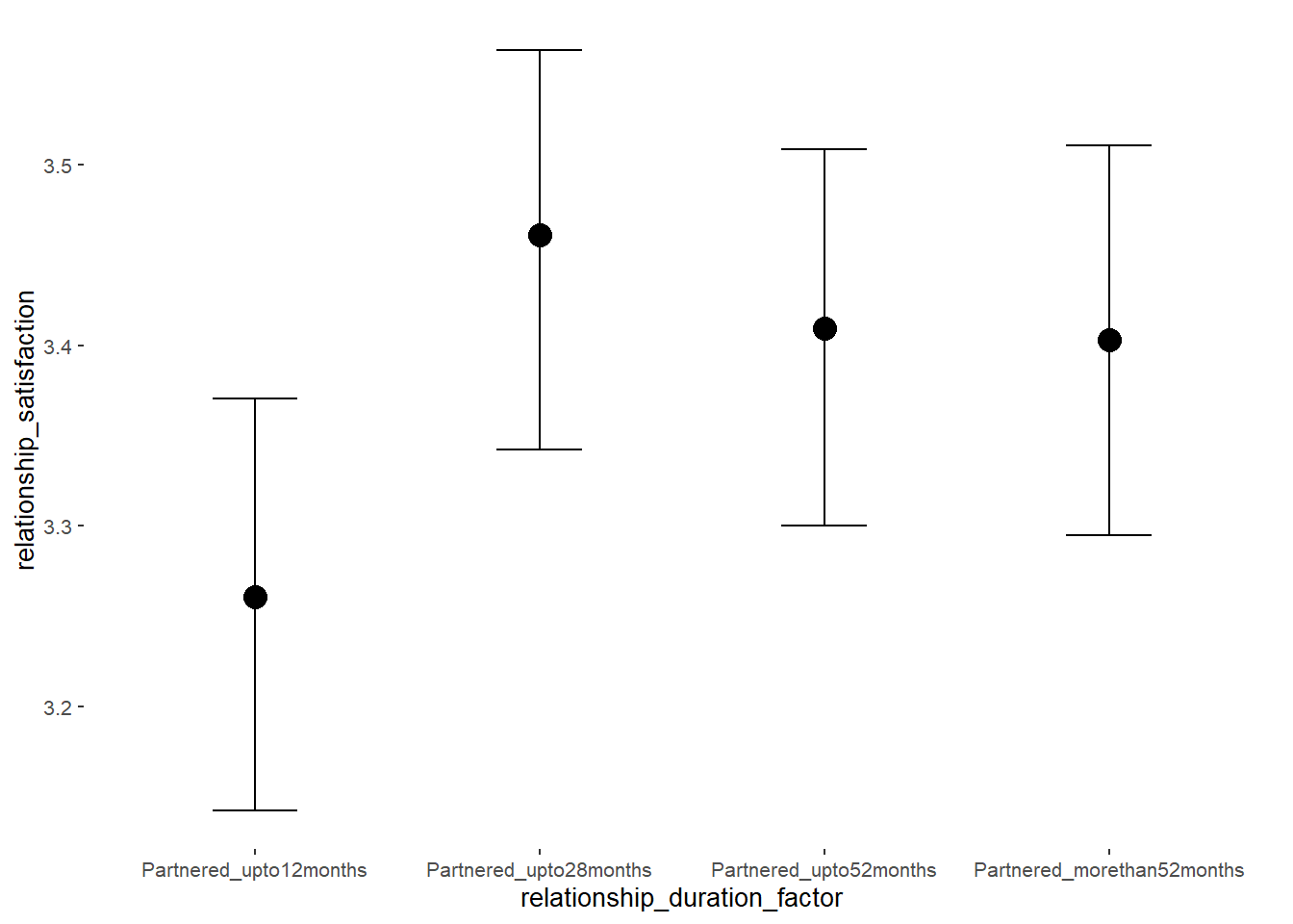


Forest Plot for Effect Sizes
m_congruency_relsat_controlled %>%

  spread_draws(b_contraception_hormonalyes, b_congruent_contraception1,
               `b_contraception_hormonalyes:congruent_contraception1`,
               b_age,
               b_net_incomeeuro_500_1000, b_net_incomeeuro_1000_2000,
               b_net_incomeeuro_2000_3000, b_net_incomeeuro_gt_3000, b_net_incomedont_tell,
               b_relationship_duration_factorPartnered_upto28months,
               b_relationship_duration_factorPartnered_upto52months,
               b_relationship_duration_factorPartnered_morethan52months,
               b_education_years,
               b_bfi_extra, b_bfi_neuro, b_bfi_agree, b_bfi_consc, b_bfi_open,
               b_religiosity) %>%
  pivot_longer(cols = c(b_contraception_hormonalyes, b_congruent_contraception1,
               `b_contraception_hormonalyes:congruent_contraception1`,
                        b_age,
               b_net_incomeeuro_500_1000, b_net_incomeeuro_1000_2000,
               b_net_incomeeuro_2000_3000, b_net_incomeeuro_gt_3000, b_net_incomedont_tell,
               b_relationship_duration_factorPartnered_upto28months,
               b_relationship_duration_factorPartnered_upto52months,
               b_relationship_duration_factorPartnered_morethan52months,
               b_education_years,
               b_bfi_extra, b_bfi_neuro, b_bfi_agree, b_bfi_consc, b_bfi_open,
               b_religiosity),
               names_to = "condition",
               values_to = "r_condition") %>%
  mutate(condition_mean = r_condition,
         group = ifelse(condition %contains% "b_relationship_duration_factor",
                        "Relationship Duration",
                        ifelse(condition %contains% "b_net_income",
                               "Income",
                               NA)),
         group = ifelse(condition %contains% "ontraception",
                        "Contraception", group),
         condition = ifelse(condition == "b_contraception_hormonalyes",
                        "Hormonal Contraception",
                     ifelse(condition == "b_congruent_contraception1",
                            "Congruent Contraception",
                     ifelse(condition == "b_contraception_hormonalyes:congruent_contraception1",
                            "Interaction Hormonal Contracpetion and Congruent Contraception",
                            condition))),
         condition = ifelse(condition == "b_age", "Age",
                ifelse(condition == "b_net_incomeeuro_500_1000", "500-1000 Euro",
                ifelse(condition == "b_net_incomeeuro_1000_2000", "1000-2000 Euro",
                ifelse(condition == "b_net_incomeeuro_2000_3000", "2000-3000 Euro",
                ifelse(condition == "b_net_incomeeuro_gt_3000", ">3000 Euro",
                ifelse(condition == "b_net_incomedont_tell", "do not tell",
                ifelse(condition == "b_relationship_duration_factorPartnered_upto28months",
                       "13-28 months",
                ifelse(condition == "b_relationship_duration_factorPartnered_upto52months",
                       "29-52 months",
                ifelse(condition == "b_relationship_duration_factorPartnered_morethan52months",
                       ">52 months",
                ifelse(condition == "b_education_years", "Years of Education",
                ifelse(condition == "b_bfi_extra", "Extraversion",
                ifelse(condition == "b_bfi_neuro", "Neuroticism",
                ifelse(condition == "b_bfi_agree", "Agreeableness",
                ifelse(condition == "b_bfi_consc", "Conscientiousness",
                ifelse(condition == "b_bfi_open", "Openness",
                ifelse(condition == "b_religiosity", "Religiosity",
                       condition)))))))))))))))),
         group = ifelse(is.na(group), condition, group),
         condition = factor(condition, levels = rev(c("Hormonal Contraception",
                                        "Congruent Contraception",
                                        "Interaction Hormonal Contracpetion and Congruent Contraception",
                                        "Age",
                                        "500-1000 Euro", "1000-2000 Euro",
                                        "2000-3000 Euro", ">3000 Euro", "do not tell",
                                        "13-28 months", "29-52 months",
                                        ">52 months",
                                        "Years of Education",
                                        "Extraversion", "Neuroticism", "Agreeableness",
                                         "Conscientiousness","Openness","Religiosity"))),
         group = factor(group, levels = c("Contraception", "Age", "Income",
                                          "Relationship Duration","Years of Education",
                                          "Extraversion", "Neuroticism", "Agreeableness",
                                         "Conscientiousness","Openness","Religiosity"))) %>%
  ggplot(aes(y = condition,
             x = condition_mean,
             fill = stat(abs(x) < 0.04))) +
  stat_halfeye() +
  geom_vline(xintercept = c(-0.04, 0.04), linetype = "dotted") +
  apatheme +
  theme(legend.position = "none") +
  scale_fill_manual(values = c("gray80", "skyblue")) +
  labs(x = "Effect Size Estimates", y = "Predictors")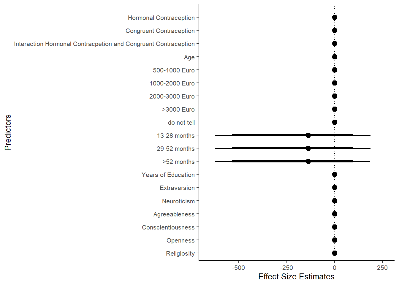
Sexual Satisfaction
Model
m_congruency_sexsat_controlled = brm(satisfaction_sexual_intercourse ~
                          contraception_hormonal * congruent_contraception +
                             age + net_income + relationship_duration_factor +
                              education_years +
                              bfi_extra + bfi_neuro + bfi_agree + bfi_consc + bfi_open +
                              religiosity,
                data = data, family = gaussian(),
                file = "m_congruency_sexsat_controlled_robust")
Summary
## Warning: Parts of the model have not converged (some Rhats are > 1.05). Be careful when analysing the results!
## We recommend running more iterations and/or setting stronger priors.
## Family: gaussian
## Links: mu = identity; sigma = identity
## Formula: satisfaction_sexual_intercourse ~ contraception_hormonal * congruent_contraception + age + net_income + relationship_duration_factor + education_years + bfi_extra + bfi_neuro + bfi_agree + bfi_consc + bfi_open + religiosity
## Data: data (Number of observations: 710)
## Draws: 4 chains, each with iter = 2000; warmup = 1000; thin = 1;
## total post-warmup draws = 4000
##
## Population-Level Effects:
## Estimate Est.Error l-90% CI u-90% CI Rhat Bulk_ESS
## Intercept 33.95 887.32 -1276.75 1540.41 3.09 5
## contraception_hormonalyes 0.22 0.12 0.04 0.42 1.14 21
## congruent_contraception1 0.08 0.10 -0.08 0.25 1.07 42
## age 0.01 0.01 -0.01 0.02 1.09 38
## net_incomeeuro_500_1000 0.03 0.12 -0.17 0.23 1.29 11
## net_incomeeuro_1000_2000 -0.03 0.14 -0.27 0.20 1.28 11
## net_incomeeuro_2000_3000 -0.03 0.19 -0.34 0.30 1.20 15
## net_incomeeuro_gt_3000 -0.19 0.31 -0.70 0.31 1.15 21
## net_incomedont_tell 0.15 0.24 -0.25 0.51 1.17 18
## relationship_duration_factorPartnered_upto12months -30.83 887.31 -1537.35 1279.32 3.09 5
## relationship_duration_factorPartnered_upto28months -30.83 887.31 -1537.40 1279.37 3.09 5
## relationship_duration_factorPartnered_upto52months -31.05 887.31 -1537.57 1279.02 3.09 5
## relationship_duration_factorPartnered_morethan52months -31.09 887.31 -1537.58 1278.98 3.09 5
## education_years -0.00 0.01 -0.02 0.01 1.13 23
## bfi_extra 0.11 0.06 0.02 0.21 1.14 30
## bfi_neuro -0.06 0.06 -0.16 0.04 1.04 54
## bfi_agree 0.16 0.07 0.03 0.28 1.06 43
## bfi_consc 0.13 0.06 0.02 0.22 1.06 52
## bfi_open -0.12 0.07 -0.22 -0.01 1.04 63
## religiosity 0.01 0.03 -0.04 0.06 1.02 74
## contraception_hormonalyes:congruent_contraception1 -0.12 0.14 -0.35 0.10 1.16 19
## Tail_ESS
## Intercept NA
## contraception_hormonalyes NA
## congruent_contraception1 NA
## age NA
## net_incomeeuro_500_1000 NA
## net_incomeeuro_1000_2000 NA
## net_incomeeuro_2000_3000 NA
## net_incomeeuro_gt_3000 NA
## net_incomedont_tell NA
## relationship_duration_factorPartnered_upto12months NA
## relationship_duration_factorPartnered_upto28months NA
## relationship_duration_factorPartnered_upto52months NA
## relationship_duration_factorPartnered_morethan52months NA
## education_years NA
## bfi_extra NA
## bfi_neuro NA
## bfi_agree NA
## bfi_consc NA
## bfi_open 125
## religiosity 157
## contraception_hormonalyes:congruent_contraception1 NA
##
## Family Specific Parameters:
## Estimate Est.Error l-90% CI u-90% CI Rhat Bulk_ESS Tail_ESS
## sigma 1.02 0.02 0.98 1.06 1.02 85 NA
##
## Draws were sampled using sampling(NUTS). For each parameter, Bulk_ESS
## and Tail_ESS are effective sample size measures, and Rhat is the potential
## scale reduction factor on split chains (at convergence, Rhat = 1).Comparison with ROPE
plot(equivalence_test(m_congruency_sexsat_controlled, range = c(-0.11, 0.11), ci = 0.90,
                      parameters = "contraception"))
## Possible multicollinearity between b_contraception_hormonalyes:congruent_contraception1 and b_contraception_hormonalyes (r = 0.73). This might lead to inappropriate results. See 'Details' in '?equivalence_test'.## Picking joint bandwidth of 0.0172## Warning: Removed 1197 rows containing non-finite values (stat_density_ridges).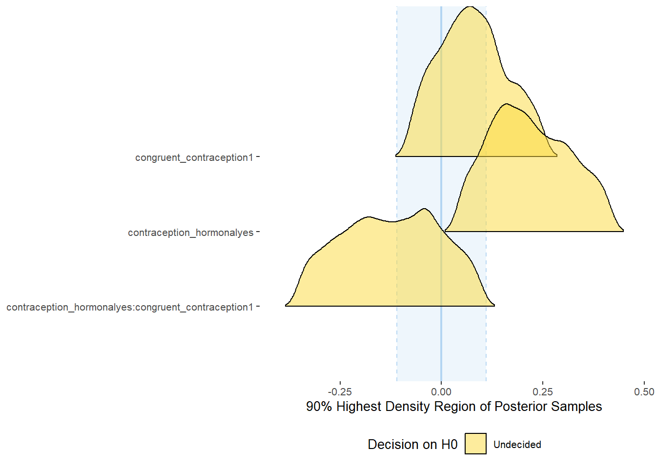
equivalence_test(m_congruency_sexsat_controlled, range = c(-0.11, 0.11), ci = 0.90,
                      parameters = "contraception")
## Possible multicollinearity between b_contraception_hormonalyes:congruent_contraception1 and b_contraception_hormonalyes (r = 0.73). This might lead to inappropriate results. See 'Details' in '?equivalence_test'.## # A tibble: 3 x 10
## Parameter CI ROPE_low ROPE_high ROPE_Percentage ROPE_Equivalence HDI_low HDI_high Effects Component
## <chr> <dbl> <dbl> <dbl> <dbl> <chr> <dbl> <dbl> <chr> <chr>
## 1 b_contraceptio~ 0.9 -0.11 0.11 0.139 Undecided 0.0396 0.418 fixed conditio~
## 2 b_congruent_co~ 0.9 -0.11 0.11 0.660 Undecided -0.0801 0.254 fixed conditio~
## 3 b_contraceptio~ 0.9 -0.11 0.11 0.469 Undecided -0.354 0.101 fixed conditio~
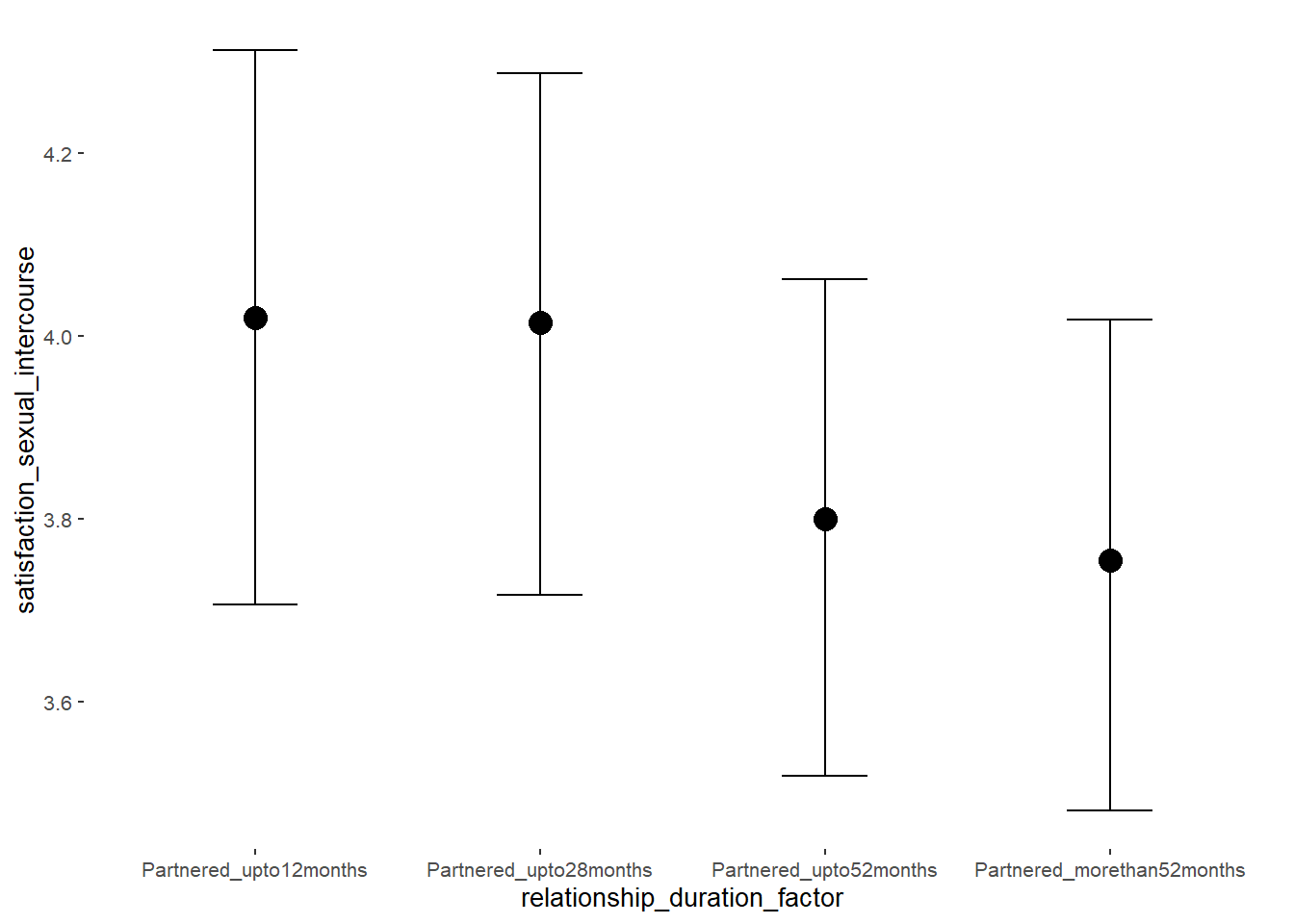


Forest Plot for Effect Sizes
m_congruency_sexsat_controlled %>%

  spread_draws(b_contraception_hormonalyes, b_congruent_contraception1,
               `b_contraception_hormonalyes:congruent_contraception1`,
               b_age,
               b_net_incomeeuro_500_1000, b_net_incomeeuro_1000_2000,
               b_net_incomeeuro_2000_3000, b_net_incomeeuro_gt_3000, b_net_incomedont_tell,
               b_relationship_duration_factorPartnered_upto28months,
               b_relationship_duration_factorPartnered_upto52months,
               b_relationship_duration_factorPartnered_morethan52months,
               b_education_years,
               b_bfi_extra, b_bfi_neuro, b_bfi_agree, b_bfi_consc, b_bfi_open,
               b_religiosity) %>%
  pivot_longer(cols = c(b_contraception_hormonalyes, b_congruent_contraception1,
               `b_contraception_hormonalyes:congruent_contraception1`,
                        b_age,
               b_net_incomeeuro_500_1000, b_net_incomeeuro_1000_2000,
               b_net_incomeeuro_2000_3000, b_net_incomeeuro_gt_3000, b_net_incomedont_tell,
               b_relationship_duration_factorPartnered_upto28months,
               b_relationship_duration_factorPartnered_upto52months,
               b_relationship_duration_factorPartnered_morethan52months,
               b_education_years,
               b_bfi_extra, b_bfi_neuro, b_bfi_agree, b_bfi_consc, b_bfi_open,
               b_religiosity),
               names_to = "condition",
               values_to = "r_condition") %>%
  mutate(condition_mean = r_condition,
         group = ifelse(condition %contains% "b_relationship_duration_factor",
                        "Relationship Duration",
                        ifelse(condition %contains% "b_net_income",
                               "Income",
                               NA)),
         group = ifelse(condition %contains% "ontraception",
                        "Contraception", group),
         condition = ifelse(condition == "b_contraception_hormonalyes",
                        "Hormonal Contraception",
                     ifelse(condition == "b_congruent_contraception1",
                            "Congruent Contraception",
                     ifelse(condition == "b_contraception_hormonalyes:congruent_contraception1",
                            "Interaction Hormonal Contracpetion and Congruent Contraception",
                            condition))),
         condition = ifelse(condition == "b_age", "Age",
                ifelse(condition == "b_net_incomeeuro_500_1000", "500-1000 Euro",
                ifelse(condition == "b_net_incomeeuro_1000_2000", "1000-2000 Euro",
                ifelse(condition == "b_net_incomeeuro_2000_3000", "2000-3000 Euro",
                ifelse(condition == "b_net_incomeeuro_gt_3000", ">3000 Euro",
                ifelse(condition == "b_net_incomedont_tell", "do not tell",
                ifelse(condition == "b_relationship_duration_factorPartnered_upto28months",
                       "13-28 months",
                ifelse(condition == "b_relationship_duration_factorPartnered_upto52months",
                       "29-52 months",
                ifelse(condition == "b_relationship_duration_factorPartnered_morethan52months",
                       ">52 months",
                ifelse(condition == "b_education_years", "Years of Education",
                ifelse(condition == "b_bfi_extra", "Extraversion",
                ifelse(condition == "b_bfi_neuro", "Neuroticism",
                ifelse(condition == "b_bfi_agree", "Agreeableness",
                ifelse(condition == "b_bfi_consc", "Conscientiousness",
                ifelse(condition == "b_bfi_open", "Openness",
                ifelse(condition == "b_religiosity", "Religiosity",
                       condition)))))))))))))))),
         group = ifelse(is.na(group), condition, group),
         condition = factor(condition, levels = rev(c("Hormonal Contraception",
                                        "Congruent Contraception",
                                        "Interaction Hormonal Contracpetion and Congruent Contraception",
                                        "Age",
                                        "500-1000 Euro", "1000-2000 Euro",
                                        "2000-3000 Euro", ">3000 Euro", "do not tell",
                                        "13-28 months", "29-52 months",
                                        ">52 months",
                                        "Years of Education",
                                        "Extraversion", "Neuroticism", "Agreeableness",
                                         "Conscientiousness","Openness","Religiosity"))),
         group = factor(group, levels = c("Contraception", "Age", "Income",
                                          "Relationship Duration","Years of Education",
                                          "Extraversion", "Neuroticism", "Agreeableness",
                                         "Conscientiousness","Openness","Religiosity"))) %>%
  ggplot(aes(y = condition,
             x = condition_mean,
             fill = stat(abs(x) < 0.11))) +
  stat_halfeye() +
  geom_vline(xintercept = c(-0.11, 0.11), linetype = "dotted") +
  apatheme +
  theme(legend.position = "none") +
  scale_fill_manual(values = c("gray80", "skyblue")) +
  labs(x = "Effect Size Estimates", y = "Predictors")
Libido
Model
m_congruency_libido_controlled = brm(diary_libido_mean ~
                          contraception_hormonal * congruent_contraception +
                             age + net_income + relationship_duration_factor +
                              education_years +
                              bfi_extra + bfi_neuro + bfi_agree + bfi_consc + bfi_open +
                              religiosity,
                data = data, family = gaussian(),
                file = "m_congruency_libido_controlled_robust")
Summary
## Warning: Parts of the model have not converged (some Rhats are > 1.05). Be careful when analysing the results!
## We recommend running more iterations and/or setting stronger priors.
## Family: gaussian
## Links: mu = identity; sigma = identity
## Formula: diary_libido_mean ~ contraception_hormonal * congruent_contraception + age + net_income + relationship_duration_factor + education_years + bfi_extra + bfi_neuro + bfi_agree + bfi_consc + bfi_open + religiosity
## Data: data (Number of observations: 586)
## Draws: 4 chains, each with iter = 2000; warmup = 1000; thin = 1;
## total post-warmup draws = 4000
##
## Population-Level Effects:
## Estimate Est.Error l-90% CI u-90% CI Rhat Bulk_ESS
## Intercept 343.12 243.60 -30.14 848.28 2.77 5
## contraception_hormonalyes -0.04 0.06 -0.13 0.05 1.13 23
## congruent_contraception1 0.02 0.06 -0.07 0.11 1.08 39
## age -0.01 0.01 -0.02 0.00 1.10 42
## net_incomeeuro_500_1000 0.12 0.05 0.04 0.20 1.12 23
## net_incomeeuro_1000_2000 0.13 0.08 0.01 0.26 1.10 30
## net_incomeeuro_2000_3000 0.18 0.10 0.02 0.34 1.10 30
## net_incomeeuro_gt_3000 0.03 0.17 -0.23 0.31 1.07 56
## net_incomedont_tell 0.32 0.15 0.09 0.58 1.11 34
## relationship_duration_factorPartnered_upto12months -341.97 243.66 -846.77 31.44 2.77 5
## relationship_duration_factorPartnered_upto28months -342.09 243.66 -846.88 31.42 2.77 5
## relationship_duration_factorPartnered_upto52months -342.11 243.66 -846.88 31.37 2.77 5
## relationship_duration_factorPartnered_morethan52months -342.14 243.67 -846.87 31.33 2.77 5
## education_years -0.00 0.01 -0.01 0.00 1.03 71
## bfi_extra 0.06 0.03 0.02 0.11 1.16 19
## bfi_neuro -0.04 0.03 -0.10 0.01 1.05 42
## bfi_agree 0.05 0.04 -0.01 0.12 1.11 38
## bfi_consc -0.09 0.03 -0.15 -0.03 1.15 23
## bfi_open 0.11 0.03 0.05 0.17 1.14 27
## religiosity -0.01 0.02 -0.03 0.02 1.02 72
## contraception_hormonalyes:congruent_contraception1 0.04 0.07 -0.09 0.15 1.14 20
## Tail_ESS
## Intercept NA
## contraception_hormonalyes NA
## congruent_contraception1 NA
## age NA
## net_incomeeuro_500_1000 NA
## net_incomeeuro_1000_2000 NA
## net_incomeeuro_2000_3000 NA
## net_incomeeuro_gt_3000 NA
## net_incomedont_tell NA
## relationship_duration_factorPartnered_upto12months NA
## relationship_duration_factorPartnered_upto28months NA
## relationship_duration_factorPartnered_upto52months NA
## relationship_duration_factorPartnered_morethan52months NA
## education_years 130
## bfi_extra NA
## bfi_neuro NA
## bfi_agree NA
## bfi_consc NA
## bfi_open NA
## religiosity NA
## contraception_hormonalyes:congruent_contraception1 NA
##
## Family Specific Parameters:
## Estimate Est.Error l-90% CI u-90% CI Rhat Bulk_ESS Tail_ESS
## sigma 0.53 0.01 0.51 0.55 1.16 21 NA
##
## Draws were sampled using sampling(NUTS). For each parameter, Bulk_ESS
## and Tail_ESS are effective sample size measures, and Rhat is the potential
## scale reduction factor on split chains (at convergence, Rhat = 1).Comparison with ROPE
plot(equivalence_test(m_congruency_libido_controlled, range = c(-0.06, 0.06), ci = 0.90,
                      parameters = "contraception"))
## Picking joint bandwidth of 0.00878## Warning: Removed 1197 rows containing non-finite values (stat_density_ridges).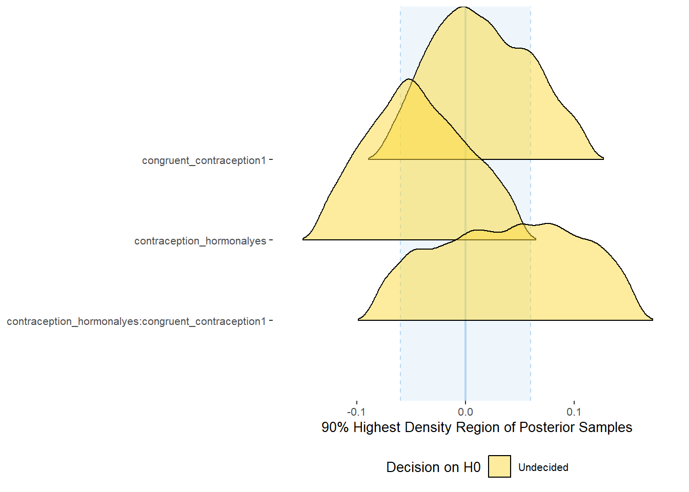
equivalence_test(m_congruency_libido_controlled, range = c(-0.06, 0.06), ci = 0.90,
                      parameters = "contraception")
## # A tibble: 3 x 10
## Parameter CI ROPE_low ROPE_high ROPE_Percentage ROPE_Equivalence HDI_low HDI_high Effects Component
## <chr> <dbl> <dbl> <dbl> <dbl> <chr> <dbl> <dbl> <chr> <chr>
## 1 b_contraceptio~ 0.9 -0.06 0.06 0.620 Undecided -0.134 0.0475 fixed conditio~
## 2 b_congruent_co~ 0.9 -0.06 0.06 0.791 Undecided -0.0741 0.111 fixed conditio~
## 3 b_contraceptio~ 0.9 -0.06 0.06 0.536 Undecided -0.0829 0.156 fixed conditio~

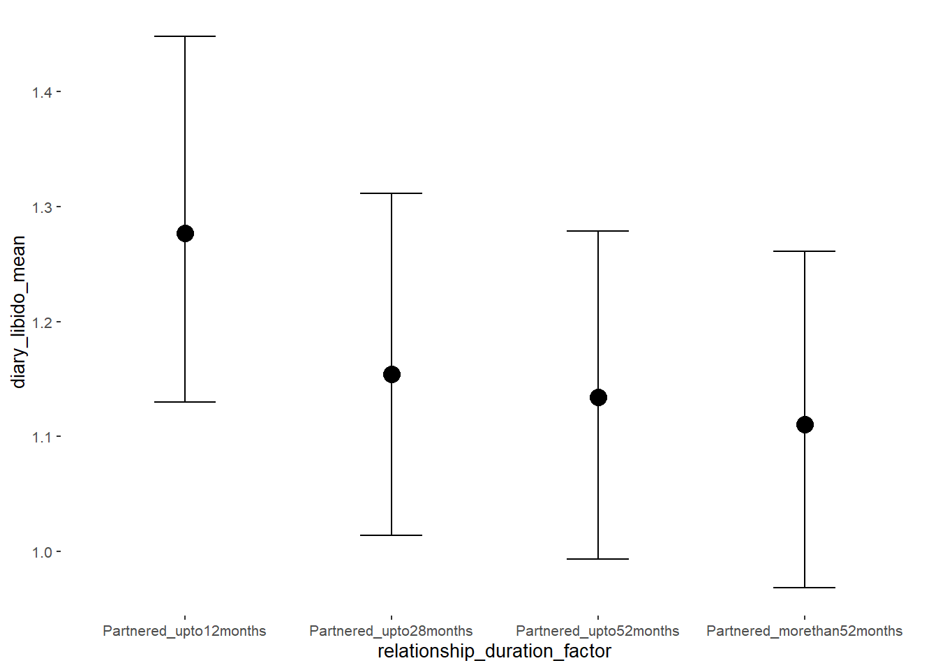


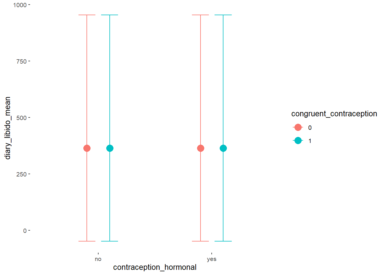
Forest Plot for Effect Sizes
m_congruency_libido_controlled %>%

  spread_draws(b_contraception_hormonalyes, b_congruent_contraception1,
               `b_contraception_hormonalyes:congruent_contraception1`,
               b_age,
               b_net_incomeeuro_500_1000, b_net_incomeeuro_1000_2000,
               b_net_incomeeuro_2000_3000, b_net_incomeeuro_gt_3000, b_net_incomedont_tell,
               b_relationship_duration_factorPartnered_upto28months,
               b_relationship_duration_factorPartnered_upto52months,
               b_relationship_duration_factorPartnered_morethan52months,
               b_education_years,
               b_bfi_extra, b_bfi_neuro, b_bfi_agree, b_bfi_consc, b_bfi_open,
               b_religiosity) %>%
  pivot_longer(cols = c(b_contraception_hormonalyes, b_congruent_contraception1,
               `b_contraception_hormonalyes:congruent_contraception1`,
                        b_age,
               b_net_incomeeuro_500_1000, b_net_incomeeuro_1000_2000,
               b_net_incomeeuro_2000_3000, b_net_incomeeuro_gt_3000, b_net_incomedont_tell,
               b_relationship_duration_factorPartnered_upto28months,
               b_relationship_duration_factorPartnered_upto52months,
               b_relationship_duration_factorPartnered_morethan52months,
               b_education_years,
               b_bfi_extra, b_bfi_neuro, b_bfi_agree, b_bfi_consc, b_bfi_open,
               b_religiosity),
               names_to = "condition",
               values_to = "r_condition") %>%
  mutate(condition_mean = r_condition,
         group = ifelse(condition %contains% "b_relationship_duration_factor",
                        "Relationship Duration",
                        ifelse(condition %contains% "b_net_income",
                               "Income",
                               NA)),
         group = ifelse(condition %contains% "ontraception",
                        "Contraception", group),
         condition = ifelse(condition == "b_contraception_hormonalyes",
                        "Hormonal Contraception",
                     ifelse(condition == "b_congruent_contraception1",
                            "Congruent Contraception",
                     ifelse(condition == "b_contraception_hormonalyes:congruent_contraception1",
                            "Interaction Hormonal Contracpetion and Congruent Contraception",
                            condition))),
         condition = ifelse(condition == "b_age", "Age",
                ifelse(condition == "b_net_incomeeuro_500_1000", "500-1000 Euro",
                ifelse(condition == "b_net_incomeeuro_1000_2000", "1000-2000 Euro",
                ifelse(condition == "b_net_incomeeuro_2000_3000", "2000-3000 Euro",
                ifelse(condition == "b_net_incomeeuro_gt_3000", ">3000 Euro",
                ifelse(condition == "b_net_incomedont_tell", "do not tell",
                ifelse(condition == "b_relationship_duration_factorPartnered_upto28months",
                       "13-28 months",
                ifelse(condition == "b_relationship_duration_factorPartnered_upto52months",
                       "29-52 months",
                ifelse(condition == "b_relationship_duration_factorPartnered_morethan52months",
                       ">52 months",
                ifelse(condition == "b_education_years", "Years of Education",
                ifelse(condition == "b_bfi_extra", "Extraversion",
                ifelse(condition == "b_bfi_neuro", "Neuroticism",
                ifelse(condition == "b_bfi_agree", "Agreeableness",
                ifelse(condition == "b_bfi_consc", "Conscientiousness",
                ifelse(condition == "b_bfi_open", "Openness",
                ifelse(condition == "b_religiosity", "Religiosity",
                       condition)))))))))))))))),
         group = ifelse(is.na(group), condition, group),
         condition = factor(condition, levels = rev(c("Hormonal Contraception",
                                        "Congruent Contraception",
                                        "Interaction Hormonal Contracpetion and Congruent Contraception",
                                        "Age",
                                        "500-1000 Euro", "1000-2000 Euro",
                                        "2000-3000 Euro", ">3000 Euro", "do not tell",
                                        "13-28 months", "29-52 months",
                                        ">52 months",
                                        "Years of Education",
                                        "Extraversion", "Neuroticism", "Agreeableness",
                                         "Conscientiousness","Openness","Religiosity"))),
         group = factor(group, levels = c("Contraception", "Age", "Income",
                                          "Relationship Duration","Years of Education",
                                          "Extraversion", "Neuroticism", "Agreeableness",
                                         "Conscientiousness","Openness","Religiosity"))) %>%
  ggplot(aes(y = condition,
             x = condition_mean,
             fill = stat(abs(x) < 0.06))) +
  stat_halfeye() +
  geom_vline(xintercept = c(-0.06, 0.06), linetype = "dotted") +
  apatheme +
  theme(legend.position = "none") +
  scale_fill_manual(values = c("gray80", "skyblue")) +
  labs(x = "Effect Size Estimates", y = "Predictors")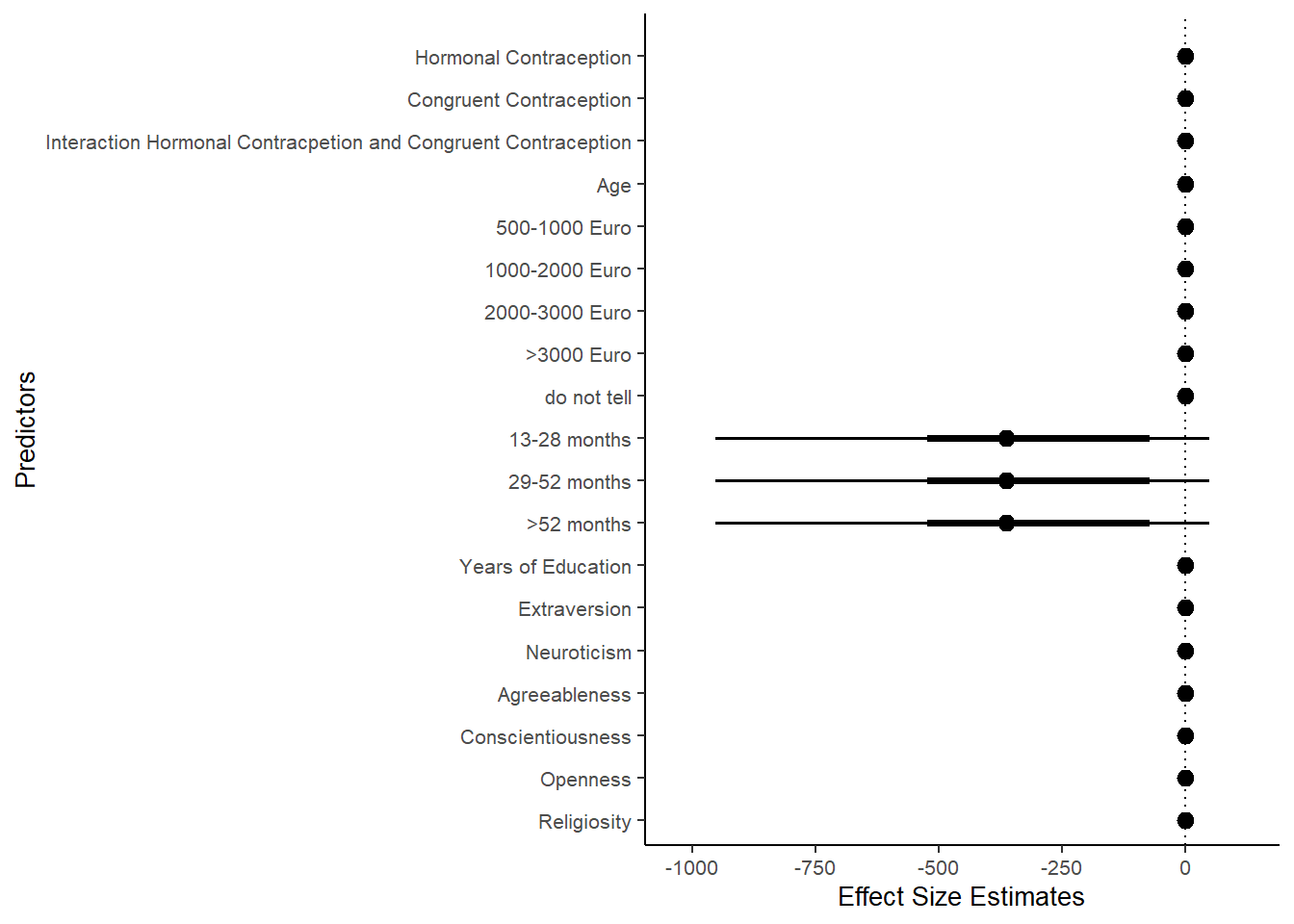
Sexual Frequency (Penetrative Intercourse)
Model
m_congruency_sexfreqpen_controlled = brm(diary_sex_active_sex_sum ~
                        offset(log(number_of_days)) +
                        contraception_hormonal * congruent_contraception +
                        age + net_income + relationship_duration_factor +
                              education_years +
                              bfi_extra + bfi_neuro + bfi_agree + bfi_consc + bfi_open +
                              religiosity,
                data = data, family = poisson(),
                file = "m_congruency_sexfreqpen_controlled_robust")
Summary
## Warning: Parts of the model have not converged (some Rhats are > 1.05). Be careful when analysing the results!
## We recommend running more iterations and/or setting stronger priors.
## Family: poisson
## Links: mu = log
## Formula: diary_sex_active_sex_sum ~ offset(log(number_of_days)) + contraception_hormonal * congruent_contraception + age + net_income + relationship_duration_factor + education_years + bfi_extra + bfi_neuro + bfi_agree + bfi_consc + bfi_open + religiosity
## Data: data (Number of observations: 576)
## Draws: 4 chains, each with iter = 2000; warmup = 1000; thin = 1;
## total post-warmup draws = 4000
##
## Population-Level Effects:
## Estimate Est.Error l-90% CI u-90% CI Rhat Bulk_ESS
## Intercept -84.42 261.19 -531.41 229.72 2.47 5
## contraception_hormonalyes 0.10 0.05 0.02 0.18 1.08 58
## congruent_contraception1 -0.04 0.04 -0.10 0.02 1.12 22
## age -0.00 0.00 -0.01 0.00 1.09 30
## net_incomeeuro_500_1000 0.13 0.03 0.07 0.19 1.09 35
## net_incomeeuro_1000_2000 0.12 0.05 0.04 0.21 1.07 33
## net_incomeeuro_2000_3000 0.43 0.06 0.34 0.54 1.05 42
## net_incomeeuro_gt_3000 0.05 0.10 -0.11 0.21 1.08 44
## net_incomedont_tell 0.41 0.09 0.25 0.54 1.12 29
## relationship_duration_factorPartnered_upto12months 82.59 261.21 -231.73 529.39 2.47 5
## relationship_duration_factorPartnered_upto28months 82.45 261.21 -231.84 529.20 2.47 5
## relationship_duration_factorPartnered_upto52months 82.20 261.21 -232.12 529.01 2.47 5
## relationship_duration_factorPartnered_morethan52months 82.20 261.21 -232.08 529.00 2.47 5
## education_years -0.01 0.00 -0.02 -0.01 1.08 74
## bfi_extra 0.00 0.02 -0.03 0.03 1.08 52
## bfi_neuro -0.01 0.02 -0.04 0.03 1.02 82
## bfi_agree 0.09 0.02 0.05 0.13 1.04 64
## bfi_consc -0.01 0.02 -0.05 0.02 1.07 44
## bfi_open 0.04 0.02 0.00 0.08 1.07 54
## religiosity -0.01 0.01 -0.03 0.00 1.09 55
## contraception_hormonalyes:congruent_contraception1 0.04 0.06 -0.05 0.14 1.10 49
## Tail_ESS
## Intercept NA
## contraception_hormonalyes NA
## congruent_contraception1 NA
## age NA
## net_incomeeuro_500_1000 NA
## net_incomeeuro_1000_2000 NA
## net_incomeeuro_2000_3000 NA
## net_incomeeuro_gt_3000 NA
## net_incomedont_tell NA
## relationship_duration_factorPartnered_upto12months NA
## relationship_duration_factorPartnered_upto28months NA
## relationship_duration_factorPartnered_upto52months NA
## relationship_duration_factorPartnered_morethan52months NA
## education_years NA
## bfi_extra NA
## bfi_neuro NA
## bfi_agree NA
## bfi_consc NA
## bfi_open NA
## religiosity NA
## contraception_hormonalyes:congruent_contraception1 NA
##
## Draws were sampled using sampling(NUTS). For each parameter, Bulk_ESS
## and Tail_ESS are effective sample size measures, and Rhat is the potential
## scale reduction factor on split chains (at convergence, Rhat = 1).Comparison with ROPE
plot(equivalence_test(m_congruency_sexfreqpen_controlled, range = c(-0.05, 0.05),
                      ci = 0.90,
                      parameters = "contraception"))
## Possible multicollinearity between b_contraception_hormonalyes:congruent_contraception1 and b_contraception_hormonalyes (r = 0.79). This might lead to inappropriate results. See 'Details' in '?equivalence_test'.## Picking joint bandwidth of 0.00639## Warning: Removed 1197 rows containing non-finite values (stat_density_ridges).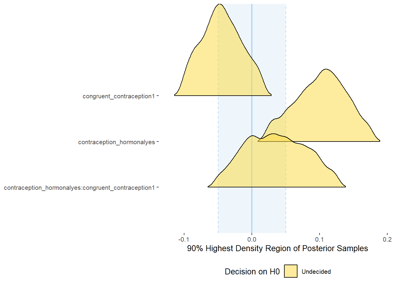
equivalence_test(m_congruency_sexfreqpen_controlled, range = c(-0.05, 0.05), ci = 0.90,
                      parameters = "contraception")
## Possible multicollinearity between b_contraception_hormonalyes:congruent_contraception1 and b_contraception_hormonalyes (r = 0.79). This might lead to inappropriate results. See 'Details' in '?equivalence_test'.## # A tibble: 3 x 10
## Parameter CI ROPE_low ROPE_high ROPE_Percentage ROPE_Equivalence HDI_low HDI_high Effects Component
## <chr> <dbl> <dbl> <dbl> <dbl> <chr> <dbl> <dbl> <chr> <chr>
## 1 b_contraceptio~ 0.9 -0.05 0.05 0.102 Undecided 0.0194 0.179 fixed conditio~
## 2 b_congruent_co~ 0.9 -0.05 0.05 0.558 Undecided -0.103 0.0173 fixed conditio~
## 3 b_contraceptio~ 0.9 -0.05 0.05 0.605 Undecided -0.0543 0.128 fixed conditio~Plots
conditional_effects(m_congruency_sexfreqpen_controlled,
                    effects = "contraception_hormonal:congruent_contraception",
                    conditions = data.frame(number_of_days = 1))
Forest Plot for Effect Sizes
m_congruency_sexfreqpen_controlled %>%

  spread_draws(b_contraception_hormonalyes, b_congruent_contraception1,
               `b_contraception_hormonalyes:congruent_contraception1`,
               b_age,
               b_net_incomeeuro_500_1000, b_net_incomeeuro_1000_2000,
               b_net_incomeeuro_2000_3000, b_net_incomeeuro_gt_3000, b_net_incomedont_tell,
               b_relationship_duration_factorPartnered_upto28months,
               b_relationship_duration_factorPartnered_upto52months,
               b_relationship_duration_factorPartnered_morethan52months,
               b_education_years,
               b_bfi_extra, b_bfi_neuro, b_bfi_agree, b_bfi_consc, b_bfi_open,
               b_religiosity) %>%
  pivot_longer(cols = c(b_contraception_hormonalyes, b_congruent_contraception1,
               `b_contraception_hormonalyes:congruent_contraception1`,
                        b_age,
               b_net_incomeeuro_500_1000, b_net_incomeeuro_1000_2000,
               b_net_incomeeuro_2000_3000, b_net_incomeeuro_gt_3000, b_net_incomedont_tell,
               b_relationship_duration_factorPartnered_upto28months,
               b_relationship_duration_factorPartnered_upto52months,
               b_relationship_duration_factorPartnered_morethan52months,
               b_education_years,
               b_bfi_extra, b_bfi_neuro, b_bfi_agree, b_bfi_consc, b_bfi_open,
               b_religiosity),
               names_to = "condition",
               values_to = "r_condition") %>%
  mutate(condition_mean = r_condition,
         group = ifelse(condition %contains% "b_relationship_duration_factor",
                        "Relationship Duration",
                        ifelse(condition %contains% "b_net_income",
                               "Income",
                               NA)),
         group = ifelse(condition %contains% "ontraception",
                        "Contraception", group),
         condition = ifelse(condition == "b_contraception_hormonalyes",
                        "Hormonal Contraception",
                     ifelse(condition == "b_congruent_contraception1",
                            "Congruent Contraception",
                     ifelse(condition == "b_contraception_hormonalyes:congruent_contraception1",
                            "Interaction Hormonal Contracpetion and Congruent Contraception",
                            condition))),
         condition = ifelse(condition == "b_age", "Age",
                ifelse(condition == "b_net_incomeeuro_500_1000", "500-1000 Euro",
                ifelse(condition == "b_net_incomeeuro_1000_2000", "1000-2000 Euro",
                ifelse(condition == "b_net_incomeeuro_2000_3000", "2000-3000 Euro",
                ifelse(condition == "b_net_incomeeuro_gt_3000", ">3000 Euro",
                ifelse(condition == "b_net_incomedont_tell", "do not tell",
                ifelse(condition == "b_relationship_duration_factorPartnered_upto28months",
                       "13-28 months",
                ifelse(condition == "b_relationship_duration_factorPartnered_upto52months",
                       "29-52 months",
                ifelse(condition == "b_relationship_duration_factorPartnered_morethan52months",
                       ">52 months",
                ifelse(condition == "b_education_years", "Years of Education",
                ifelse(condition == "b_bfi_extra", "Extraversion",
                ifelse(condition == "b_bfi_neuro", "Neuroticism",
                ifelse(condition == "b_bfi_agree", "Agreeableness",
                ifelse(condition == "b_bfi_consc", "Conscientiousness",
                ifelse(condition == "b_bfi_open", "Openness",
                ifelse(condition == "b_religiosity", "Religiosity",
                       condition)))))))))))))))),
         group = ifelse(is.na(group), condition, group),
         condition = factor(condition, levels = rev(c("Hormonal Contraception",
                                        "Congruent Contraception",
                                        "Interaction Hormonal Contracpetion and Congruent Contraception",
                                        "Age",
                                        "500-1000 Euro", "1000-2000 Euro",
                                        "2000-3000 Euro", ">3000 Euro", "do not tell",
                                        "13-28 months", "29-52 months",
                                        ">52 months",
                                        "Years of Education",
                                        "Extraversion", "Neuroticism", "Agreeableness",
                                         "Conscientiousness","Openness","Religiosity"))),
         group = factor(group, levels = c("Contraception", "Age", "Income",
                                          "Relationship Duration","Years of Education",
                                          "Extraversion", "Neuroticism", "Agreeableness",
                                         "Conscientiousness","Openness","Religiosity"))) %>%
  ggplot(aes(y = condition,
             x = condition_mean,
             fill = stat(abs(x) < 0.05))) +
  stat_halfeye() +
  geom_vline(xintercept = c(-0.05, 0.05), linetype = "dotted") +
  apatheme +
  theme(legend.position = "none") +
  scale_fill_manual(values = c("gray80", "skyblue")) +
  labs(x = "Effect Size Estimates", y = "Predictors")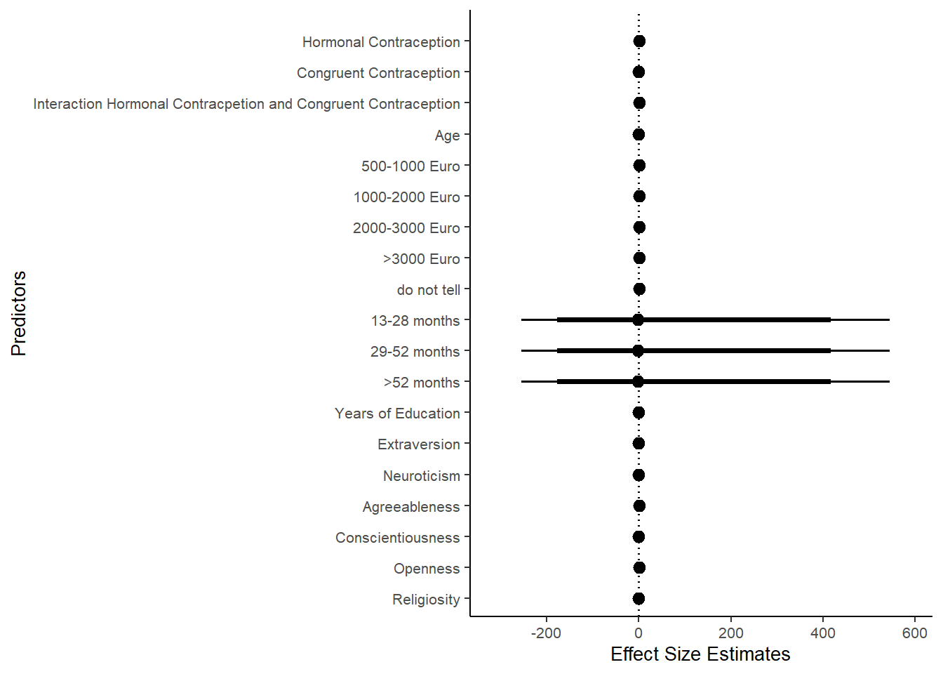
Masturbation Frequency
Model
m_congruency_masfreq_controlled = brm(diary_masturbation_sum ~
                        offset(log(number_of_days)) +
                        contraception_hormonal * congruent_contraception +
                        age + net_income + relationship_duration_factor +
                              education_years +
                              bfi_extra + bfi_neuro + bfi_agree + bfi_consc + bfi_open +
                              religiosity,
                data = data, family = poisson(),
                file = "m_congruency_masfreq_controlled_robust")
Summary
## Warning: Parts of the model have not converged (some Rhats are > 1.05). Be careful when analysing the results!
## We recommend running more iterations and/or setting stronger priors.
## Family: poisson
## Links: mu = log
## Formula: diary_masturbation_sum ~ offset(log(number_of_days)) + contraception_hormonal * congruent_contraception + age + net_income + relationship_duration_factor + education_years + bfi_extra + bfi_neuro + bfi_agree + bfi_consc + bfi_open + religiosity
## Data: data (Number of observations: 576)
## Draws: 4 chains, each with iter = 2000; warmup = 1000; thin = 1;
## total post-warmup draws = 4000
##
## Population-Level Effects:
## Estimate Est.Error l-90% CI u-90% CI Rhat Bulk_ESS
## Intercept 293.71 229.91 -68.01 653.35 3.26 4
## contraception_hormonalyes -0.43 0.06 -0.54 -0.34 1.24 12
## congruent_contraception1 0.03 0.05 -0.05 0.10 1.18 17
## age -0.01 0.00 -0.02 -0.00 1.13 29
## net_incomeeuro_500_1000 0.18 0.04 0.13 0.25 1.13 22
## net_incomeeuro_1000_2000 0.23 0.06 0.14 0.33 1.14 37
## net_incomeeuro_2000_3000 -0.01 0.08 -0.15 0.13 1.13 35
## net_incomeeuro_gt_3000 -0.11 0.16 -0.39 0.13 1.16 22
## net_incomedont_tell -0.17 0.13 -0.40 0.06 1.12 25
## relationship_duration_factorPartnered_upto12months -295.30 229.88 -655.14 66.12 3.26 4
## relationship_duration_factorPartnered_upto28months -295.26 229.88 -655.06 66.24 3.26 4
## relationship_duration_factorPartnered_upto52months -295.36 229.88 -655.19 66.12 3.26 4
## relationship_duration_factorPartnered_morethan52months -295.50 229.88 -655.36 65.93 3.26 4
## education_years 0.00 0.00 -0.00 0.01 1.09 43
## bfi_extra -0.03 0.02 -0.07 0.00 1.09 41
## bfi_neuro -0.01 0.02 -0.06 0.03 1.15 19
## bfi_agree -0.00 0.03 -0.06 0.04 1.18 19
## bfi_consc -0.23 0.02 -0.27 -0.19 1.34 10
## bfi_open 0.22 0.03 0.17 0.26 1.19 18
## religiosity -0.04 0.01 -0.06 -0.02 1.11 29
## contraception_hormonalyes:congruent_contraception1 0.12 0.07 -0.00 0.25 1.27 12
## Tail_ESS
## Intercept NA
## contraception_hormonalyes NA
## congruent_contraception1 NA
## age NA
## net_incomeeuro_500_1000 NA
## net_incomeeuro_1000_2000 NA
## net_incomeeuro_2000_3000 NA
## net_incomeeuro_gt_3000 NA
## net_incomedont_tell NA
## relationship_duration_factorPartnered_upto12months NA
## relationship_duration_factorPartnered_upto28months NA
## relationship_duration_factorPartnered_upto52months NA
## relationship_duration_factorPartnered_morethan52months NA
## education_years NA
## bfi_extra NA
## bfi_neuro NA
## bfi_agree NA
## bfi_consc NA
## bfi_open NA
## religiosity NA
## contraception_hormonalyes:congruent_contraception1 NA
##
## Draws were sampled using sampling(NUTS). For each parameter, Bulk_ESS
## and Tail_ESS are effective sample size measures, and Rhat is the potential
## scale reduction factor on split chains (at convergence, Rhat = 1).Comparison with ROPE
plot(equivalence_test(m_congruency_masfreq_controlled, range = c(-0.05, 0.05), ci = 0.90,
                      parameters = "contraception"))
## Possible multicollinearity between b_contraception_hormonalyes:congruent_contraception1 and b_contraception_hormonalyes (r = 0.76). This might lead to inappropriate results. See 'Details' in '?equivalence_test'.## Picking joint bandwidth of 0.00785## Warning: Removed 1197 rows containing non-finite values (stat_density_ridges).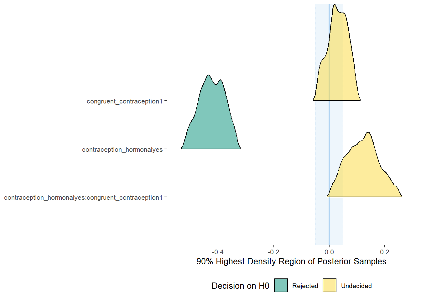
equivalence_test(m_congruency_masfreq_controlled, range = c(-0.05, 0.05), ci = 0.90,
                      parameters = "contraception")
## Possible multicollinearity between b_contraception_hormonalyes:congruent_contraception1 and b_contraception_hormonalyes (r = 0.76). This might lead to inappropriate results. See 'Details' in '?equivalence_test'.## # A tibble: 3 x 10
## Parameter CI ROPE_low ROPE_high ROPE_Percentage ROPE_Equivalence HDI_low HDI_high Effects Component
## <chr> <dbl> <dbl> <dbl> <dbl> <chr> <dbl> <dbl> <chr> <chr>
## 1 b_contracepti~ 0.9 -0.05 0.05 0 Rejected -0.522 -0.333 fixed conditio~
## 2 b_congruent_c~ 0.9 -0.05 0.05 0.671 Undecided -0.0431 0.0992 fixed conditio~
## 3 b_contracepti~ 0.9 -0.05 0.05 0.116 Undecided 0.00524 0.251 fixed conditio~Plots
conditional_effects(m_congruency_masfreq_controlled,
                    effects = "contraception_hormonal:congruent_contraception",
                    conditions = data.frame(number_of_days = 1))
Forest Plot for Effect Sizes
m_congruency_masfreq_controlled %>%

  spread_draws(b_contraception_hormonalyes, b_congruent_contraception1,
               `b_contraception_hormonalyes:congruent_contraception1`,
               b_age,
               b_net_incomeeuro_500_1000, b_net_incomeeuro_1000_2000,
               b_net_incomeeuro_2000_3000, b_net_incomeeuro_gt_3000, b_net_incomedont_tell,
               b_relationship_duration_factorPartnered_upto28months,
               b_relationship_duration_factorPartnered_upto52months,
               b_relationship_duration_factorPartnered_morethan52months,
               b_education_years,
               b_bfi_extra, b_bfi_neuro, b_bfi_agree, b_bfi_consc, b_bfi_open,
               b_religiosity) %>%
  pivot_longer(cols = c(b_contraception_hormonalyes, b_congruent_contraception1,
               `b_contraception_hormonalyes:congruent_contraception1`,
                        b_age,
               b_net_incomeeuro_500_1000, b_net_incomeeuro_1000_2000,
               b_net_incomeeuro_2000_3000, b_net_incomeeuro_gt_3000, b_net_incomedont_tell,
               b_relationship_duration_factorPartnered_upto28months,
               b_relationship_duration_factorPartnered_upto52months,
               b_relationship_duration_factorPartnered_morethan52months,
               b_education_years,
               b_bfi_extra, b_bfi_neuro, b_bfi_agree, b_bfi_consc, b_bfi_open,
               b_religiosity),
               names_to = "condition",
               values_to = "r_condition") %>%
  mutate(condition_mean = r_condition,
         group = ifelse(condition %contains% "b_relationship_duration_factor",
                        "Relationship Duration",
                        ifelse(condition %contains% "b_net_income",
                               "Income",
                               NA)),
         group = ifelse(condition %contains% "ontraception",
                        "Contraception", group),
         condition = ifelse(condition == "b_contraception_hormonalyes",
                        "Hormonal Contraception",
                     ifelse(condition == "b_congruent_contraception1",
                            "Congruent Contraception",
                     ifelse(condition == "b_contraception_hormonalyes:congruent_contraception1",
                            "Interaction Hormonal Contracpetion and Congruent Contraception",
                            condition))),
         condition = ifelse(condition == "b_age", "Age",
                ifelse(condition == "b_net_incomeeuro_500_1000", "500-1000 Euro",
                ifelse(condition == "b_net_incomeeuro_1000_2000", "1000-2000 Euro",
                ifelse(condition == "b_net_incomeeuro_2000_3000", "2000-3000 Euro",
                ifelse(condition == "b_net_incomeeuro_gt_3000", ">3000 Euro",
                ifelse(condition == "b_net_incomedont_tell", "do not tell",
                ifelse(condition == "b_relationship_duration_factorPartnered_upto28months",
                       "13-28 months",
                ifelse(condition == "b_relationship_duration_factorPartnered_upto52months",
                       "29-52 months",
                ifelse(condition == "b_relationship_duration_factorPartnered_morethan52months",
                       ">52 months",
                ifelse(condition == "b_education_years", "Years of Education",
                ifelse(condition == "b_bfi_extra", "Extraversion",
                ifelse(condition == "b_bfi_neuro", "Neuroticism",
                ifelse(condition == "b_bfi_agree", "Agreeableness",
                ifelse(condition == "b_bfi_consc", "Conscientiousness",
                ifelse(condition == "b_bfi_open", "Openness",
                ifelse(condition == "b_religiosity", "Religiosity",
                       condition)))))))))))))))),
         group = ifelse(is.na(group), condition, group),
         condition = factor(condition, levels = rev(c("Hormonal Contraception",
                                        "Congruent Contraception",
                                        "Interaction Hormonal Contracpetion and Congruent Contraception",
                                        "Age",
                                        "500-1000 Euro", "1000-2000 Euro",
                                        "2000-3000 Euro", ">3000 Euro", "do not tell",
                                        "13-28 months", "29-52 months",
                                        ">52 months",
                                        "Years of Education",
                                        "Extraversion", "Neuroticism", "Agreeableness",
                                         "Conscientiousness","Openness","Religiosity"))),
         group = factor(group, levels = c("Contraception", "Age", "Income",
                                          "Relationship Duration","Years of Education",
                                          "Extraversion", "Neuroticism", "Agreeableness",
                                         "Conscientiousness","Openness","Religiosity"))) %>%
  ggplot(aes(y = condition,
             x = condition_mean,
             fill = stat(abs(x) < 0.05))) +
  stat_halfeye() +
  geom_vline(xintercept = c(-0.05, 0.05), linetype = "dotted") +
  apatheme +
  theme(legend.position = "none") +
  scale_fill_manual(values = c("gray80", "skyblue")) +
  labs(x = "Effect Size Estimates", y = "Predictors")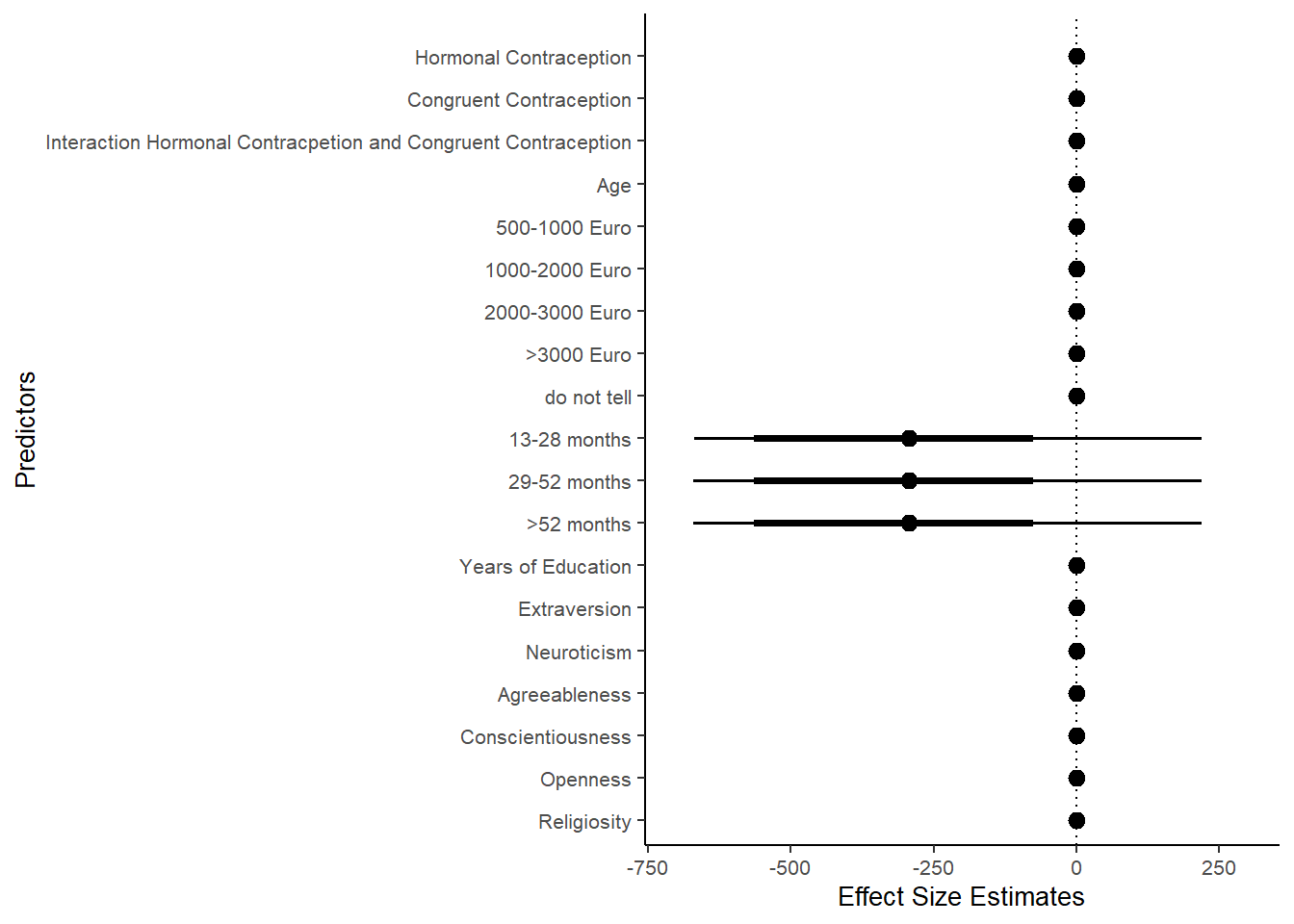
Model Comparison
Attractiveness of partner
LooIC first model: 1563.68
LooIC second model: 1564.32
Model Comparisons: The difference between models is -0.32 compared to a standard error of 1.99
## Output of model 'm_hc_atrr':
##
## Computed from 4000 by 710 log-likelihood matrix
##
##          Estimate   SE
## elpd_loo   -781.8 20.5
## p_loo         3.1  0.3
## looic      1563.7 40.9
## ------
## Monte Carlo SE of elpd_loo is 0.0.
##
## All Pareto k estimates are good (k < 0.5).
## See help('pareto-k-diagnostic') for details.
##
## Output of model 'm_congruency_atrr':
##
## Computed from 4000 by 710 log-likelihood matrix
##
##          Estimate   SE
## elpd_loo   -782.2 20.7
## p_loo         5.2  0.4
## looic      1564.3 41.3
## ------
## Monte Carlo SE of elpd_loo is 0.0.
##
## All Pareto k estimates are good (k < 0.5).
## See help('pareto-k-diagnostic') for details.
##
## Model comparisons:
##                   elpd_diff se_diff
## m_hc_atrr          0.0       0.0
## m_congruency_atrr -0.3       2.0
Relationship satisfaction
LooIC first model: 795.66
LooIC second model: 792.98
Model Comparisons: The difference between models is -1.34 compared to a standard error of 2.63
## Output of model 'm_hc_relsat':
##
## Computed from 4000 by 710 log-likelihood matrix
##
##          Estimate   SE
## elpd_loo   -397.8 25.0
## p_loo         3.7  0.5
## looic       795.7 50.1
## ------
## Monte Carlo SE of elpd_loo is 0.0.
##
## All Pareto k estimates are good (k < 0.5).
## See help('pareto-k-diagnostic') for details.
##
## Output of model 'm_congruency_relsat':
##
## Computed from 4000 by 710 log-likelihood matrix
##
##          Estimate   SE
## elpd_loo   -396.5 24.7
## p_loo         5.5  0.6
## looic       793.0 49.3
## ------
## Monte Carlo SE of elpd_loo is 0.0.
##
## All Pareto k estimates are good (k < 0.5).
## See help('pareto-k-diagnostic') for details.
##
## Model comparisons:
##                     elpd_diff se_diff
## m_congruency_relsat  0.0       0.0
## m_hc_relsat         -1.3       2.6
Sexual Satisfaction
m_hc_sexsat$data$satisfaction_sexual_intercourse =
  as.numeric(m_hc_sexsat$data$satisfaction_sexual_intercourse)
m_congruency_sexsat$data$satisfaction_sexual_intercourse =
  as.numeric(m_congruency_sexsat$data$satisfaction_sexual_intercourse)

compare_models = loo(m_hc_sexsat, m_congruency_sexsat)
LooIC first model: 2070.32
LooIC second model: 2072.21
Model Comparisons: The difference between models is -0.94 compared to a standard error of 1.57
## Output of model 'm_hc_sexsat':
##
## Computed from 4000 by 710 log-likelihood matrix
##
##          Estimate   SE
## elpd_loo  -1035.2 19.9
## p_loo         3.2  0.3
## looic      2070.3 39.8
## ------
## Monte Carlo SE of elpd_loo is 0.0.
##
## All Pareto k estimates are good (k < 0.5).
## See help('pareto-k-diagnostic') for details.
##
## Output of model 'm_congruency_sexsat':
##
## Computed from 4000 by 710 log-likelihood matrix
##
##          Estimate   SE
## elpd_loo  -1036.1 20.0
## p_loo         5.1  0.4
## looic      2072.2 39.9
## ------
## Monte Carlo SE of elpd_loo is 0.0.
##
## All Pareto k estimates are good (k < 0.5).
## See help('pareto-k-diagnostic') for details.
##
## Model comparisons:
##                     elpd_diff se_diff
## m_hc_sexsat          0.0       0.0
## m_congruency_sexsat -0.9       1.6
LS0tDQp0aXRsZTogIlJvYnVzdG5lc3MgQW5hbHlzZXMgRWZmZWN0cyBvZiBDb250cmFjZXB0aW9uIg0Kb3V0cHV0Og0KICBodG1sX2RvY3VtZW50Og0KICAgIHRvYzogdHJ1ZQ0KICAgIHRvY19kZXB0aDogNA0KICAgIHRvY19mbG9hdDogdHJ1ZQ0KICAgIGNvZGVfZm9sZGluZzogJ2hpZGUnDQogICAgc2VsZl9jb250YWluZWQ6IGZhbHNlDQplZGl0b3Jfb3B0aW9uczogDQogIGNodW5rX291dHB1dF90eXBlOiBjb25zb2xlDQotLS0NCiAgDQogIA0KIyMgRGF0YSANCmBgYHtyIHJlc3VsdHM9J2hpZGUnLG1lc3NhZ2U9Rix3YXJuaW5nPUZ9DQpzb3VyY2UoIjBfaGVscGVycy5SIikNCg0KbG9hZCgiZGF0YS9jbGVhbmVkX3NlbGVjdGVkX3dyYW5nbGVkLnJkYXRhIikNCg0KZGF0YSA9IGRhdGEgJT4lDQogIGZpbHRlcighKGNvbnRyYWNlcHRpb25fbWV0aG9kICVjb250YWlucyUgImhvcm1vbmFsX290aGVyIikpDQpgYGANCg0KDQojIyBFZmZlY3RzIG9mIEhvcm1vbmFsIENvbnRyYWNlcHRpdmVzIHsudGFic2V0fQ0KIyMjIEF0dHJhY3RpdmVuZXNzIG9mIFBhcnRuZXIgey50YWJzZXR9DQojIyMjIE1vZGVsDQpgYGB7cn0NCm1faGNfYXRyciA9IGJybShhdHRyYWN0aXZlbmVzc19wYXJ0bmVyIH4gY29udHJhY2VwdGlvbl9ob3Jtb25hbCwNCiAgICAgICAgICAgICAgICBkYXRhID0gZGF0YSwgZmFtaWx5ID0gZ2F1c3NpYW4oKSwNCiAgICAgICAgICAgICAgICBmaWxlID0gIm1faGNfYXRycl9yb2J1c3QiKQ0KYGBgDQoNCiMjIyMgU3VtbWFyeQ0KYGBge3J9DQpzdW1tYXJ5KG1faGNfYXRyciwgY29uZi5pbnQgPSBULCBwcm9iID0gMC45MCkNCmBgYA0KDQojIyMjIENvbXBhcmlzb24gd2l0aCBST1BFDQpgYGB7cn0NCnBsb3QoZXF1aXZhbGVuY2VfdGVzdChtX2hjX2F0cnIsIHJhbmdlID0gYygtMC4wNywgMC4wNyksIGNpID0gMC45MCwNCiAgICAgICAgICAgICAgICAgICAgICBwYXJhbWV0ZXJzID0gImNvbnRyYWNlcHRpb24iKSkNCmVxdWl2YWxlbmNlX3Rlc3QobV9oY19hdHJyLCByYW5nZSA9IGMoLTAuMDcsIDAuMDcpLCBjaSA9IDAuOTAsDQogICAgICAgICAgICAgICAgICAgICAgcGFyYW1ldGVycyA9ICJjb250cmFjZXB0aW9uIikNCmBgYA0KDQojIyMjIFBsb3RzDQpgYGB7ciB3YXJuaW5nID0gRkFMU0V9DQpjb25kaXRpb25hbF9lZmZlY3RzKG1faGNfYXRyciwgYXNrID0gRkFMU0UpDQpgYGANCg0KIyMjIyBGb3Jlc3QgUGxvdCBmb3IgRWZmZWN0IFNpemVzIHsuYWN0aXZlfQ0KYGBge3J9DQptX2hjX2F0cnIgJT4lDQogIHNwcmVhZF9kcmF3cyhiX2NvbnRyYWNlcHRpb25faG9ybW9uYWx5ZXMpICU+JQ0KICBwaXZvdF9sb25nZXIoY29scyA9IGMoYl9jb250cmFjZXB0aW9uX2hvcm1vbmFseWVzKSwNCiAgICAgICAgICAgICAgIG5hbWVzX3RvID0gImNvbmRpdGlvbiIsDQogICAgICAgICAgICAgICB2YWx1ZXNfdG8gPSAicl9jb25kaXRpb24iKSAlPiUNCiAgbXV0YXRlKGNvbmRpdGlvbl9tZWFuID0gcl9jb25kaXRpb24sDQogICAgICAgICBncm91cCA9IGlmZWxzZShjb25kaXRpb24gJWNvbnRhaW5zJSAiYl9jb250cmFjZXB0aW9uX2hvcm1vbmFseWVzIiwNCiAgICAgICAgICAgICAgICAgICAgICAgICJDb250cmFjZXB0aW9uIiwgTkEpLA0KICAgICAgICAgY29uZGl0aW9uID0gaWZlbHNlKGNvbmRpdGlvbiAlY29udGFpbnMlICJiX2NvbnRyYWNlcHRpb25faG9ybW9uYWx5ZXMiLA0KICAgICAgICAgICAgICAgICAgICAgICAgIkhvcm1vbmFsIENvbnRyYWNlcHRpb24iLCBOQSkpICU+JQ0KICBnZ3Bsb3QoYWVzKHkgPSBjb25kaXRpb24sDQogICAgICAgICAgICAgeCA9IGNvbmRpdGlvbl9tZWFuLA0KICAgICAgICAgICAgIGZpbGwgPSBzdGF0KGFicyh4KSA8IDAuMDcpKSkgKw0KICBzdGF0X2hhbGZleWUoKSArDQogIGdlb21fdmxpbmUoeGludGVyY2VwdCA9IGMoLTAuMDcsIDAuMDcpLCBsaW5ldHlwZSA9ICJkb3R0ZWQiKSArDQogIGFwYXRoZW1lICsNCiAgdGhlbWUobGVnZW5kLnBvc2l0aW9uID0gIm5vbmUiKSArDQogIHNjYWxlX2ZpbGxfbWFudWFsKHZhbHVlcyA9IGMoImdyYXk4MCIsICJza3libHVlIikpICsNCiAgbGFicyh4ID0gIkVmZmVjdCBTaXplIEVzdGltYXRlcyIsIHkgPSAiUHJlZGljdG9ycyIpICsNCiAgeGxpbSAoLTAuNiwgMC42KQ0KYGBgDQoNCiMjIyBSZWxhdGlvbnNoaXAgU2F0aXNmYWN0aW9uIHsudGFic2V0fQ0KIyMjIyBNb2RlbA0KYGBge3J9DQptX2hjX3JlbHNhdCA9IGJybShyZWxhdGlvbnNoaXBfc2F0aXNmYWN0aW9uIH4gY29udHJhY2VwdGlvbl9ob3Jtb25hbCwNCiAgICAgICAgICAgICAgICBkYXRhID0gZGF0YSwgZmFtaWx5ID0gZ2F1c3NpYW4oKSwNCiAgICAgICAgICAgICAgICBmaWxlID0gIm1faGNfcmVsc2F0X3JvYnVzdCIpDQpgYGANCg0KIyMjIyBTdW1tYXJ5DQpgYGB7cn0NCnN1bW1hcnkobV9oY19yZWxzYXQsIGNvbmYuaW50ID0gVCwgcHJvYiA9IDAuOTApDQpgYGANCg0KIyMjIyBDb21wYXJpc29uIHdpdGggUk9QRQ0KYGBge3J9DQpwbG90KGVxdWl2YWxlbmNlX3Rlc3QobV9oY19yZWxzYXQsIHJhbmdlID0gYygtMC4wNCwgMC4wNCksIGNpID0gMC45MCwNCiAgICAgICAgICAgICAgICAgICAgICBwYXJhbWV0ZXJzID0gImNvbnRyYWNlcHRpb24iKSkNCmVxdWl2YWxlbmNlX3Rlc3QobV9oY19yZWxzYXQsIHJhbmdlID0gYygtMC4wNCwgMC4wNCksIGNpID0gMC45MCwNCiAgICAgICAgICAgICAgICAgICAgICBwYXJhbWV0ZXJzID0gImNvbnRyYWNlcHRpb24iKQ0KYGBgDQoNCiMjIyMgUGxvdHMNCmBgYHtyIHdhcm5pbmcgPSBGQUxTRX0NCmNvbmRpdGlvbmFsX2VmZmVjdHMobV9oY19yZWxzYXQsIGFzayA9IEZBTFNFKQ0KYGBgDQoNCiMjIyMgRm9yZXN0IFBsb3QgZm9yIEVmZmVjdCBTaXplcyB7LmFjdGl2ZX0NCmBgYHtyfQ0KbV9oY19yZWxzYXQgJT4lDQogIHNwcmVhZF9kcmF3cyhiX2NvbnRyYWNlcHRpb25faG9ybW9uYWx5ZXMpICU+JQ0KICBwaXZvdF9sb25nZXIoY29scyA9IGMoYl9jb250cmFjZXB0aW9uX2hvcm1vbmFseWVzKSwNCiAgICAgICAgICAgICAgIG5hbWVzX3RvID0gImNvbmRpdGlvbiIsDQogICAgICAgICAgICAgICB2YWx1ZXNfdG8gPSAicl9jb25kaXRpb24iKSAlPiUNCiAgbXV0YXRlKGNvbmRpdGlvbl9tZWFuID0gcl9jb25kaXRpb24sDQogICAgICAgICBncm91cCA9IGlmZWxzZShjb25kaXRpb24gJWNvbnRhaW5zJSAiYl9jb250cmFjZXB0aW9uX2hvcm1vbmFseWVzIiwNCiAgICAgICAgICAgICAgICAgICAgICAgICJDb250cmFjZXB0aW9uIiwgTkEpLA0KICAgICAgICAgY29uZGl0aW9uID0gaWZlbHNlKGNvbmRpdGlvbiAlY29udGFpbnMlICJiX2NvbnRyYWNlcHRpb25faG9ybW9uYWx5ZXMiLA0KICAgICAgICAgICAgICAgICAgICAgICAgIkhvcm1vbmFsIENvbnRyYWNlcHRpb24iLCBOQSkpICU+JQ0KICBnZ3Bsb3QoYWVzKHkgPSBjb25kaXRpb24sDQogICAgICAgICAgICAgeCA9IGNvbmRpdGlvbl9tZWFuLA0KICAgICAgICAgICAgIGZpbGwgPSBzdGF0KGFicyh4KSA8IDAuMDQpKSkgKw0KICBzdGF0X2hhbGZleWUoKSArDQogIGdlb21fdmxpbmUoeGludGVyY2VwdCA9IGMoLTAuMDQsIDAuMDQpLCBsaW5ldHlwZSA9ICJkb3R0ZWQiKSArDQogIGFwYXRoZW1lICsNCiAgdGhlbWUobGVnZW5kLnBvc2l0aW9uID0gIm5vbmUiKSArDQogIHNjYWxlX2ZpbGxfbWFudWFsKHZhbHVlcyA9IGMoImdyYXk4MCIsICJza3libHVlIikpICsNCiAgbGFicyh4ID0gIkVmZmVjdCBTaXplIEVzdGltYXRlcyIsIHkgPSAiUHJlZGljdG9ycyIpICsNCiAgeGxpbSAoLTAuNiwgMC42KQ0KYGBgDQoNCg0KIyMjIFNleHVhbCBTYXRpc2ZhY3Rpb24gey50YWJzZXR9DQojIyMjIE1vZGVsDQpgYGB7cn0NCm1faGNfc2V4c2F0ID0gYnJtKHNhdGlzZmFjdGlvbl9zZXh1YWxfaW50ZXJjb3Vyc2UgfiBjb250cmFjZXB0aW9uX2hvcm1vbmFsLA0KICAgICAgICAgICAgICAgIGRhdGEgPSBkYXRhLCBmYW1pbHkgPSBnYXVzc2lhbigpLA0KICAgICAgICAgICAgICAgIGZpbGUgPSAibV9oY19zZXhzYXRfcm9idXN0IikNCmBgYA0KDQojIyMjIFN1bW1hcnkNCmBgYHtyfQ0Kc3VtbWFyeShtX2hjX3NleHNhdCwgY29uZi5pbnQgPSBULCBwcm9iID0gMC45MCkNCmBgYA0KDQojIyMjIENvbXBhcmlzb24gd2l0aCBST1BFDQpgYGB7cn0NCnBsb3QoZXF1aXZhbGVuY2VfdGVzdChtX2hjX3NleHNhdCwgcmFuZ2UgPSBjKC0wLjExLCAwLjExKSwgY2kgPSAwLjkwLA0KICAgICAgICAgICAgICAgICAgICAgIHBhcmFtZXRlcnMgPSAiY29udHJhY2VwdGlvbiIpKQ0KZXF1aXZhbGVuY2VfdGVzdChtX2hjX3NleHNhdCwgcmFuZ2UgPSBjKC0wLjExLCAwLjExKSwgY2kgPSAwLjkwLA0KICAgICAgICAgICAgICAgICAgICAgIHBhcmFtZXRlcnMgPSAiY29udHJhY2VwdGlvbiIpDQpgYGANCg0KIyMjIyBQbG90cw0KYGBge3Igd2FybmluZyA9IEZBTFNFfQ0KY29uZGl0aW9uYWxfZWZmZWN0cyhtX2hjX3NleHNhdCwgYXNrID0gRkFMU0UpDQpgYGANCg0KIyMjIyBGb3Jlc3QgUGxvdCBmb3IgRWZmZWN0IFNpemVzIHsuYWN0aXZlfQ0KYGBge3J9DQptX2hjX3NleHNhdCAlPiUNCiAgc3ByZWFkX2RyYXdzKGJfY29udHJhY2VwdGlvbl9ob3Jtb25hbHllcykgJT4lDQogIHBpdm90X2xvbmdlcihjb2xzID0gYyhiX2NvbnRyYWNlcHRpb25faG9ybW9uYWx5ZXMpLA0KICAgICAgICAgICAgICAgbmFtZXNfdG8gPSAiY29uZGl0aW9uIiwNCiAgICAgICAgICAgICAgIHZhbHVlc190byA9ICJyX2NvbmRpdGlvbiIpICU+JQ0KICBtdXRhdGUoY29uZGl0aW9uX21lYW4gPSByX2NvbmRpdGlvbiwNCiAgICAgICAgIGdyb3VwID0gaWZlbHNlKGNvbmRpdGlvbiAlY29udGFpbnMlICJiX2NvbnRyYWNlcHRpb25faG9ybW9uYWx5ZXMiLA0KICAgICAgICAgICAgICAgICAgICAgICAgIkNvbnRyYWNlcHRpb24iLCBOQSksDQogICAgICAgICBjb25kaXRpb24gPSBpZmVsc2UoY29uZGl0aW9uICVjb250YWlucyUgImJfY29udHJhY2VwdGlvbl9ob3Jtb25hbHllcyIsDQogICAgICAgICAgICAgICAgICAgICAgICAiSG9ybW9uYWwgQ29udHJhY2VwdGlvbiIsIE5BKSkgJT4lDQogIGdncGxvdChhZXMoeSA9IGNvbmRpdGlvbiwNCiAgICAgICAgICAgICB4ID0gY29uZGl0aW9uX21lYW4sDQogICAgICAgICAgICAgZmlsbCA9IHN0YXQoYWJzKHgpIDwgMC4xMSkpKSArDQogIHN0YXRfaGFsZmV5ZSgpICsNCiAgZ2VvbV92bGluZSh4aW50ZXJjZXB0ID0gYygtMC4xMSwgMC4xMSksIGxpbmV0eXBlID0gImRvdHRlZCIpICsNCiAgYXBhdGhlbWUgKw0KICB0aGVtZShsZWdlbmQucG9zaXRpb24gPSAibm9uZSIpICsNCiAgc2NhbGVfZmlsbF9tYW51YWwodmFsdWVzID0gYygiZ3JheTgwIiwgInNreWJsdWUiKSkgKw0KICBsYWJzKHggPSAiRWZmZWN0IFNpemUgRXN0aW1hdGVzIiwgeSA9ICJQcmVkaWN0b3JzIikgKw0KICB4bGltICgtMC42LCAwLjYpDQpgYGANCg0KIyMjIExpYmlkbyB7LnRhYnNldH0NCg0KIyMjIyBNb2RlbA0KYGBge3J9DQptX2hjX2xpYmlkbyA9IGJybShkaWFyeV9saWJpZG9fbWVhbiB+IGNvbnRyYWNlcHRpb25faG9ybW9uYWwsDQogICAgICAgICAgICAgICAgZGF0YSA9IGRhdGEsIGZhbWlseSA9IGdhdXNzaWFuKCksDQogICAgICAgICAgICAgICAgZmlsZSA9ICJtX2hjX2xpYmlkb19yb2J1c3QiKQ0KYGBgDQoNCiMjIyMgU3VtbWFyeQ0KYGBge3J9DQpzdW1tYXJ5KG1faGNfbGliaWRvLCBjb25mLmludCA9IFQsIHByb2IgPSAwLjkwKQ0KYGBgDQoNCiMjIyMgQ29tcGFyaXNvbiB3aXRoIFJPUEUNCmBgYHtyfQ0KcGxvdChlcXVpdmFsZW5jZV90ZXN0KG1faGNfbGliaWRvLCByYW5nZSA9IGMoLTAuMDYsIDAuMDYpLCBjaSA9IDAuOTAsDQogICAgICAgICAgICAgICAgICAgICAgcGFyYW1ldGVycyA9ICJjb250cmFjZXB0aW9uIikpDQplcXVpdmFsZW5jZV90ZXN0KG1faGNfbGliaWRvLCByYW5nZSA9IGMoLTAuMDYsIDAuMDYpLCBjaSA9IDAuOTAsDQogICAgICAgICAgICAgICAgICAgICAgcGFyYW1ldGVycyA9ICJjb250cmFjZXB0aW9uIikNCmBgYA0KDQojIyMjIFBsb3RzDQpgYGB7ciB3YXJuaW5nID0gRkFMU0V9DQpjb25kaXRpb25hbF9lZmZlY3RzKG1faGNfbGliaWRvLCBhc2sgPSBGQUxTRSkNCmBgYA0KDQojIyMjIEZvcmVzdCBQbG90IGZvciBFZmZlY3QgU2l6ZXMgey5hY3RpdmV9DQpgYGB7cn0NCm1faGNfbGliaWRvICU+JQ0KICBzcHJlYWRfZHJhd3MoYl9jb250cmFjZXB0aW9uX2hvcm1vbmFseWVzKSAlPiUNCiAgcGl2b3RfbG9uZ2VyKGNvbHMgPSBjKGJfY29udHJhY2VwdGlvbl9ob3Jtb25hbHllcyksDQogICAgICAgICAgICAgICBuYW1lc190byA9ICJjb25kaXRpb24iLA0KICAgICAgICAgICAgICAgdmFsdWVzX3RvID0gInJfY29uZGl0aW9uIikgJT4lDQogIG11dGF0ZShjb25kaXRpb25fbWVhbiA9IHJfY29uZGl0aW9uLA0KICAgICAgICAgZ3JvdXAgPSBpZmVsc2UoY29uZGl0aW9uICVjb250YWlucyUgImJfY29udHJhY2VwdGlvbl9ob3Jtb25hbHllcyIsDQogICAgICAgICAgICAgICAgICAgICAgICAiQ29udHJhY2VwdGlvbiIsIE5BKSwNCiAgICAgICAgIGNvbmRpdGlvbiA9IGlmZWxzZShjb25kaXRpb24gJWNvbnRhaW5zJSAiYl9jb250cmFjZXB0aW9uX2hvcm1vbmFseWVzIiwNCiAgICAgICAgICAgICAgICAgICAgICAgICJIb3Jtb25hbCBDb250cmFjZXB0aW9uIiwgTkEpKSAlPiUNCiAgZ2dwbG90KGFlcyh5ID0gY29uZGl0aW9uLA0KICAgICAgICAgICAgIHggPSBjb25kaXRpb25fbWVhbiwNCiAgICAgICAgICAgICBmaWxsID0gc3RhdChhYnMoeCkgPCAwLjA2KSkpICsNCiAgc3RhdF9oYWxmZXllKCkgKw0KICBnZW9tX3ZsaW5lKHhpbnRlcmNlcHQgPSBjKC0wLjA2LCAwLjA2KSwgbGluZXR5cGUgPSAiZG90dGVkIikgKw0KICBhcGF0aGVtZSArDQogIHRoZW1lKGxlZ2VuZC5wb3NpdGlvbiA9ICJub25lIikgKw0KICBzY2FsZV9maWxsX21hbnVhbCh2YWx1ZXMgPSBjKCJncmF5ODAiLCAic2t5Ymx1ZSIpKSArDQogIGxhYnMoeCA9ICJFZmZlY3QgU2l6ZSBFc3RpbWF0ZXMiLCB5ID0gIlByZWRpY3RvcnMiKSArDQogIHhsaW0gKC0wLjYsIDAuNikNCmBgYA0KDQojIyMgU2V4dWFsIEZyZXF1ZW5jeSAoUGVuZXRyYXRpdmUgSW50ZXJjb3Vyc2UpIHsudGFic2V0fQ0KIyMjIyBNb2RlbA0KYGBge3J9DQptX2hjX3NleGZyZXFwZW4gPSBicm0oZGlhcnlfc2V4X2FjdGl2ZV9zZXhfc3VtIH4NCiAgICAgICAgICAgICAgICAgICAgICAgIG9mZnNldChsb2cobnVtYmVyX29mX2RheXMpKSArDQogICAgICAgICAgICAgICAgICAgICAgICBjb250cmFjZXB0aW9uX2hvcm1vbmFsLA0KICAgICAgICAgICAgICAgIGRhdGEgPSBkYXRhLCBmYW1pbHkgPSBwb2lzc29uKCksDQogICAgICAgICAgICAgICAgZmlsZSA9ICJtX2hjX3NleGZyZXFwZW5fcm9idXN0IikNCmBgYA0KDQojIyMjIFN1bW1hcnkNCmBgYHtyfQ0Kc3VtbWFyeShtX2hjX3NleGZyZXFwZW4sIGNvbmYuaW50ID0gVCwgcHJvYiA9IDAuOTApDQpgYGANCg0KIyMjIyBDb21wYXJpc29uIHdpdGggUk9QRQ0KYGBge3J9DQpwbG90KGVxdWl2YWxlbmNlX3Rlc3QobV9oY19zZXhmcmVxcGVuLCByYW5nZSA9IGMoLTAuMDUsIDAuMDUpKSwgY2kgPSAwLjkwLA0KICAgICAgICAgICAgICAgICAgICAgIHBhcmFtZXRlcnMgPSAiY29udHJhY2VwdGlvbiIpDQplcXVpdmFsZW5jZV90ZXN0KG1faGNfc2V4ZnJlcXBlbiwgcmFuZ2UgPSBjKC0wLjA1LCAwLjA1KSwgY2kgPSAwLjkwLA0KICAgICAgICAgICAgICAgICAgICAgIHBhcmFtZXRlcnMgPSAiY29udHJhY2VwdGlvbiIpDQpgYGANCg0KIyMjIyBQbG90cw0KYGBge3Igd2FybmluZyA9IEZBTFNFfQ0KY29uZGl0aW9uYWxfZWZmZWN0cyhtX2hjX3NleGZyZXFwZW4sDQogICAgICAgICAgICAgICAgICAgIGVmZmVjdHMgPSAiY29udHJhY2VwdGlvbl9ob3Jtb25hbCIsDQogICAgICAgICAgICAgICAgICAgIGNvbmRpdGlvbnMgPSBkYXRhLmZyYW1lKG51bWJlcl9vZl9kYXlzID0gMSkpDQpgYGANCg0KIyMjIyBGb3Jlc3QgUGxvdCBmb3IgRWZmZWN0IFNpemVzIHsuYWN0aXZlfQ0KYGBge3J9DQptX2hjX3NleGZyZXFwZW4gJT4lDQogIHNwcmVhZF9kcmF3cyhiX2NvbnRyYWNlcHRpb25faG9ybW9uYWx5ZXMpICU+JQ0KICBwaXZvdF9sb25nZXIoY29scyA9IGMoYl9jb250cmFjZXB0aW9uX2hvcm1vbmFseWVzKSwNCiAgICAgICAgICAgICAgIG5hbWVzX3RvID0gImNvbmRpdGlvbiIsDQogICAgICAgICAgICAgICB2YWx1ZXNfdG8gPSAicl9jb25kaXRpb24iKSAlPiUNCiAgbXV0YXRlKGNvbmRpdGlvbl9tZWFuID0gcl9jb25kaXRpb24sDQogICAgICAgICBncm91cCA9IGlmZWxzZShjb25kaXRpb24gJWNvbnRhaW5zJSAiYl9jb250cmFjZXB0aW9uX2hvcm1vbmFseWVzIiwNCiAgICAgICAgICAgICAgICAgICAgICAgICJDb250cmFjZXB0aW9uIiwgTkEpLA0KICAgICAgICAgY29uZGl0aW9uID0gaWZlbHNlKGNvbmRpdGlvbiAlY29udGFpbnMlICJiX2NvbnRyYWNlcHRpb25faG9ybW9uYWx5ZXMiLA0KICAgICAgICAgICAgICAgICAgICAgICAgIkhvcm1vbmFsIENvbnRyYWNlcHRpb24iLCBOQSkpICU+JQ0KICBnZ3Bsb3QoYWVzKHkgPSBjb25kaXRpb24sDQogICAgICAgICAgICAgeCA9IGNvbmRpdGlvbl9tZWFuLA0KICAgICAgICAgICAgIGZpbGwgPSBzdGF0KGFicyh4KSA8IDAuMDUpKSkgKw0KICBzdGF0X2hhbGZleWUoKSArDQogIGdlb21fdmxpbmUoeGludGVyY2VwdCA9IGMoLTAuMDUsIDAuMDUpLCBsaW5ldHlwZSA9ICJkb3R0ZWQiKSArDQogIGFwYXRoZW1lICsNCiAgdGhlbWUobGVnZW5kLnBvc2l0aW9uID0gIm5vbmUiKSArDQogIHNjYWxlX2ZpbGxfbWFudWFsKHZhbHVlcyA9IGMoImdyYXk4MCIsICJza3libHVlIikpICsNCiAgbGFicyh4ID0gIkVmZmVjdCBTaXplIEVzdGltYXRlcyIsIHkgPSAiUHJlZGljdG9ycyIpDQpgYGANCg0KIyMjIE1hc3R1cmJhdGlvbiBGcmVxdWVuY3kgey50YWJzZXR9DQojIyMjIE1vZGVsDQpgYGB7cn0NCm1faGNfbWFzZnJlcSA9IGJybShkaWFyeV9tYXN0dXJiYXRpb25fc3VtIH4gb2Zmc2V0KGxvZyhudW1iZXJfb2ZfZGF5cykpICsNCiAgICAgICAgICAgICAgICAgICAgIGNvbnRyYWNlcHRpb25faG9ybW9uYWwsDQogICAgICAgICAgICAgICAgZGF0YSA9IGRhdGEsIGZhbWlseSA9IHBvaXNzb24oKSwNCiAgICAgICAgICAgICAgICBmaWxlID0gIm1faGNfbWFzZnJlcV9yb2J1c3QiKQ0KYGBgDQoNCiMjIyMgU3VtbWFyeQ0KYGBge3J9DQpzdW1tYXJ5KG1faGNfbWFzZnJlcSwgY29uZi5pbnQgPSBULCBwcm9iID0gMC45MCkNCmBgYA0KDQojIyMjIENvbXBhcmlzb24gd2l0aCBST1BFDQpgYGB7cn0NCnBsb3QoZXF1aXZhbGVuY2VfdGVzdChtX2hjX21hc2ZyZXEsIHJhbmdlID0gYygtMC4wNSwgMC4wNSksIGNpID0gMC45MCwNCiAgICAgICAgICAgICAgICAgICAgICBwYXJhbWV0ZXJzID0gImNvbnRyYWNlcHRpb24iKSkNCmVxdWl2YWxlbmNlX3Rlc3QobV9oY19tYXNmcmVxLCByYW5nZSA9IGMoLTAuMDUsIDAuMDUpLCBjaSA9IDAuOTAsDQogICAgICAgICAgICAgICAgICAgICAgcGFyYW1ldGVycyA9ICJjb250cmFjZXB0aW9uIikNCmBgYA0KDQojIyMjIFBsb3RzDQpgYGB7ciB3YXJuaW5nID0gRkFMU0V9DQpjb25kaXRpb25hbF9lZmZlY3RzKG1faGNfbWFzZnJlcSwNCiAgICAgICAgICAgICAgICAgICAgZWZmZWN0cyA9ICJjb250cmFjZXB0aW9uX2hvcm1vbmFsIiwNCiAgICAgICAgICAgICAgICAgICAgY29uZGl0aW9ucyA9IGRhdGEuZnJhbWUobnVtYmVyX29mX2RheXMgPSAxKSkNCmBgYA0KDQojIyMjIEZvcmVzdCBQbG90IGZvciBFZmZlY3QgU2l6ZXMgey5hY3RpdmV9DQpgYGB7cn0NCm1faGNfbWFzZnJlcSAlPiUNCiAgc3ByZWFkX2RyYXdzKGJfY29udHJhY2VwdGlvbl9ob3Jtb25hbHllcykgJT4lDQogIHBpdm90X2xvbmdlcihjb2xzID0gYyhiX2NvbnRyYWNlcHRpb25faG9ybW9uYWx5ZXMpLA0KICAgICAgICAgICAgICAgbmFtZXNfdG8gPSAiY29uZGl0aW9uIiwNCiAgICAgICAgICAgICAgIHZhbHVlc190byA9ICJyX2NvbmRpdGlvbiIpICU+JQ0KICBtdXRhdGUoY29uZGl0aW9uX21lYW4gPSByX2NvbmRpdGlvbiwNCiAgICAgICAgIGdyb3VwID0gaWZlbHNlKGNvbmRpdGlvbiAlY29udGFpbnMlICJiX2NvbnRyYWNlcHRpb25faG9ybW9uYWx5ZXMiLA0KICAgICAgICAgICAgICAgICAgICAgICAgIkNvbnRyYWNlcHRpb24iLCBOQSksDQogICAgICAgICBjb25kaXRpb24gPSBpZmVsc2UoY29uZGl0aW9uICVjb250YWlucyUgImJfY29udHJhY2VwdGlvbl9ob3Jtb25hbHllcyIsDQogICAgICAgICAgICAgICAgICAgICAgICAiSG9ybW9uYWwgQ29udHJhY2VwdGlvbiIsIE5BKSkgJT4lDQogIGdncGxvdChhZXMoeSA9IGNvbmRpdGlvbiwNCiAgICAgICAgICAgICB4ID0gY29uZGl0aW9uX21lYW4sDQogICAgICAgICAgICAgZmlsbCA9IHN0YXQoYWJzKHgpIDwgMC4wNSkpKSArDQogIHN0YXRfaGFsZmV5ZSgpICsNCiAgZ2VvbV92bGluZSh4aW50ZXJjZXB0ID0gYygtMC4wNSwgMC4wNSksIGxpbmV0eXBlID0gImRvdHRlZCIpICsNCiAgYXBhdGhlbWUgKw0KICB0aGVtZShsZWdlbmQucG9zaXRpb24gPSAibm9uZSIpICsNCiAgc2NhbGVfZmlsbF9tYW51YWwodmFsdWVzID0gYygiZ3JheTgwIiwgInNreWJsdWUiKSkgKw0KICBsYWJzKHggPSAiRWZmZWN0IFNpemUgRXN0aW1hdGVzIiwgeSA9ICJQcmVkaWN0b3JzIikNCmBgYA0KDQojIyBDb250cm9sbGVkIE1vZGVsczogRWZmZWN0cyBvZiBIb3Jtb25hbCBDb250cmFjZXB0aXZlcyB7LnRhYnNldH0NCiMjIyBBdHRyYWN0aXZlbmVzcyBvZiBQYXJ0bmVyIHsudGFic2V0fQ0KIyMjIyBNb2RlbA0KYGBge3J9DQptX2hjX2F0cnJfY29udHJvbGxlZCA9IGJybShhdHRyYWN0aXZlbmVzc19wYXJ0bmVyIH4gY29udHJhY2VwdGlvbl9ob3Jtb25hbCArDQogICAgICAgICAgICAgICAgICAgICAgICAgICAgIGFnZSArIG5ldF9pbmNvbWUgKyByZWxhdGlvbnNoaXBfZHVyYXRpb25fZmFjdG9yICsNCiAgICAgICAgICAgICAgICAgICAgICAgICAgICAgIGVkdWNhdGlvbl95ZWFycyArDQogICAgICAgICAgICAgICAgICAgICAgICAgICAgICBiZmlfZXh0cmEgKyBiZmlfbmV1cm8gKyBiZmlfYWdyZWUgKyBiZmlfY29uc2MgKyBiZmlfb3BlbiArDQogICAgICAgICAgICAgICAgICAgICAgICAgICAgICByZWxpZ2lvc2l0eSwNCiAgICAgICAgICAgICAgICBkYXRhID0gZGF0YSwgZmFtaWx5ID0gZ2F1c3NpYW4oKSwNCiAgICAgICAgICAgICAgICBmaWxlID0gIm1faGNfYXRycl9jb250cm9sbGVkX3JvYnVzdCIpDQpgYGANCg0KIyMjIyBTdW1tYXJ5DQpgYGB7cn0NCnN1bW1hcnkobV9oY19hdHJyX2NvbnRyb2xsZWQsIGNvbmYuaW50ID0gVCwgcHJvYiA9IDAuOTApDQpgYGANCg0KIyMjIyBDb21wYXJpc29uIHdpdGggUk9QRQ0KYGBge3J9DQpwbG90KGVxdWl2YWxlbmNlX3Rlc3QobV9oY19hdHJyX2NvbnRyb2xsZWQsIHJhbmdlID0gYygtMC4wNywgMC4wNyksIGNpID0gMC45MCwNCiAgICAgICAgICAgICAgICAgICAgICBwYXJhbWV0ZXJzID0gImNvbnRyYWNlcHRpb24iKSkNCmVxdWl2YWxlbmNlX3Rlc3QobV9oY19hdHJyX2NvbnRyb2xsZWQsIHJhbmdlID0gYygtMC4wNywgMC4wNyksIGNpID0gMC45MCwNCiAgICAgICAgICAgICAgICAgICAgICBwYXJhbWV0ZXJzID0gImNvbnRyYWNlcHRpb24iKQ0KYGBgDQoNCiMjIyMgUGxvdHMNCmBgYHtyIHdhcm5pbmcgPSBGQUxTRX0NCmNvbmRpdGlvbmFsX2VmZmVjdHMobV9oY19hdHJyLCBhc2sgPSBGQUxTRSkNCmBgYA0KDQojIyMjIEZvcmVzdCBQbG90IGZvciBFZmZlY3QgU2l6ZXMgey5hY3RpdmV9DQpgYGB7cn0NCm1faGNfYXRycl9jb250cm9sbGVkICU+JQ0KICBzcHJlYWRfZHJhd3MoYl9jb250cmFjZXB0aW9uX2hvcm1vbmFseWVzLA0KICAgICAgICAgICAgICAgYl9hZ2UsDQogICAgICAgICAgICAgICBiX25ldF9pbmNvbWVldXJvXzUwMF8xMDAwLCBiX25ldF9pbmNvbWVldXJvXzEwMDBfMjAwMCwgDQogICAgICAgICAgICAgICBiX25ldF9pbmNvbWVldXJvXzIwMDBfMzAwMCwgYl9uZXRfaW5jb21lZXVyb19ndF8zMDAwLCBiX25ldF9pbmNvbWVkb250X3RlbGwsDQogICAgICAgICAgICAgICBiX3JlbGF0aW9uc2hpcF9kdXJhdGlvbl9mYWN0b3JQYXJ0bmVyZWRfdXB0bzI4bW9udGhzLA0KICAgICAgICAgICAgICAgYl9yZWxhdGlvbnNoaXBfZHVyYXRpb25fZmFjdG9yUGFydG5lcmVkX3VwdG81Mm1vbnRocywNCiAgICAgICAgICAgICAgIGJfcmVsYXRpb25zaGlwX2R1cmF0aW9uX2ZhY3RvclBhcnRuZXJlZF9tb3JldGhhbjUybW9udGhzLA0KICAgICAgICAgICAgICAgYl9lZHVjYXRpb25feWVhcnMsDQogICAgICAgICAgICAgICBiX2JmaV9leHRyYSwgYl9iZmlfbmV1cm8sIGJfYmZpX2FncmVlLCBiX2JmaV9jb25zYywgYl9iZmlfb3BlbiwgDQogICAgICAgICAgICAgICBiX3JlbGlnaW9zaXR5KSAlPiUNCiAgcGl2b3RfbG9uZ2VyKGNvbHMgPSBjKGJfY29udHJhY2VwdGlvbl9ob3Jtb25hbHllcywNCiAgICAgICAgICAgICAgICAgICAgICAgIGJfYWdlLA0KICAgICAgICAgICAgICAgYl9uZXRfaW5jb21lZXVyb181MDBfMTAwMCwgYl9uZXRfaW5jb21lZXVyb18xMDAwXzIwMDAsIA0KICAgICAgICAgICAgICAgYl9uZXRfaW5jb21lZXVyb18yMDAwXzMwMDAsIGJfbmV0X2luY29tZWV1cm9fZ3RfMzAwMCwgYl9uZXRfaW5jb21lZG9udF90ZWxsLA0KICAgICAgICAgICAgICAgYl9yZWxhdGlvbnNoaXBfZHVyYXRpb25fZmFjdG9yUGFydG5lcmVkX3VwdG8yOG1vbnRocywNCiAgICAgICAgICAgICAgIGJfcmVsYXRpb25zaGlwX2R1cmF0aW9uX2ZhY3RvclBhcnRuZXJlZF91cHRvNTJtb250aHMsDQogICAgICAgICAgICAgICBiX3JlbGF0aW9uc2hpcF9kdXJhdGlvbl9mYWN0b3JQYXJ0bmVyZWRfbW9yZXRoYW41Mm1vbnRocywNCiAgICAgICAgICAgICAgIGJfZWR1Y2F0aW9uX3llYXJzLA0KICAgICAgICAgICAgICAgYl9iZmlfZXh0cmEsIGJfYmZpX25ldXJvLCBiX2JmaV9hZ3JlZSwgYl9iZmlfY29uc2MsIGJfYmZpX29wZW4sIA0KICAgICAgICAgICAgICAgYl9yZWxpZ2lvc2l0eSksDQogICAgICAgICAgICAgICBuYW1lc190byA9ICJjb25kaXRpb24iLA0KICAgICAgICAgICAgICAgdmFsdWVzX3RvID0gInJfY29uZGl0aW9uIikgJT4lDQogIG11dGF0ZShjb25kaXRpb25fbWVhbiA9IHJfY29uZGl0aW9uLA0KICAgICAgICAgZ3JvdXAgPSBpZmVsc2UoY29uZGl0aW9uICVjb250YWlucyUgImJfcmVsYXRpb25zaGlwX2R1cmF0aW9uX2ZhY3RvciIsDQogICAgICAgICAgICAgICAgICAgICAgICAiUmVsYXRpb25zaGlwIER1cmF0aW9uIiwNCiAgICAgICAgICAgICAgICAgICAgICAgIGlmZWxzZShjb25kaXRpb24gJWNvbnRhaW5zJSAiYl9uZXRfaW5jb21lIiwNCiAgICAgICAgICAgICAgICAgICAgICAgICAgICAgICAiSW5jb21lIiwNCiAgICAgICAgICAgICAgICAgICAgICAgICAgICAgICBOQSkpLA0KICAgICAgICAgZ3JvdXAgPSBpZmVsc2UoY29uZGl0aW9uICVjb250YWlucyUgImJfY29udHJhY2VwdGlvbl9ob3Jtb25hbHllcyIsDQogICAgICAgICAgICAgICAgICAgICAgICAiQ29udHJhY2VwdGlvbiIsIGdyb3VwKSwNCiAgICAgICAgIGNvbmRpdGlvbiA9IGlmZWxzZShjb25kaXRpb24gJWNvbnRhaW5zJSAiYl9jb250cmFjZXB0aW9uX2hvcm1vbmFseWVzIiwNCiAgICAgICAgICAgICAgICAgICAgICAgICJIb3Jtb25hbCBDb250cmFjZXB0aW9uIiwgY29uZGl0aW9uKSwNCiAgICAgICAgIGNvbmRpdGlvbiA9IGlmZWxzZShjb25kaXRpb24gPT0gImJfYWdlIiwgIkFnZSIsDQogICAgICAgICAgICAgICAgaWZlbHNlKGNvbmRpdGlvbiA9PSAiYl9uZXRfaW5jb21lZXVyb181MDBfMTAwMCIsICI1MDAtMTAwMCBFdXJvIiwNCiAgICAgICAgICAgICAgICBpZmVsc2UoY29uZGl0aW9uID09ICJiX25ldF9pbmNvbWVldXJvXzEwMDBfMjAwMCIsICIxMDAwLTIwMDAgRXVybyIsDQogICAgICAgICAgICAgICAgaWZlbHNlKGNvbmRpdGlvbiA9PSAiYl9uZXRfaW5jb21lZXVyb18yMDAwXzMwMDAiLCAiMjAwMC0zMDAwIEV1cm8iLA0KICAgICAgICAgICAgICAgIGlmZWxzZShjb25kaXRpb24gPT0gImJfbmV0X2luY29tZWV1cm9fZ3RfMzAwMCIsICI+MzAwMCBFdXJvIiwNCiAgICAgICAgICAgICAgICBpZmVsc2UoY29uZGl0aW9uID09ICJiX25ldF9pbmNvbWVkb250X3RlbGwiLCAiZG8gbm90IHRlbGwiLA0KICAgICAgICAgICAgICAgIGlmZWxzZShjb25kaXRpb24gPT0gImJfcmVsYXRpb25zaGlwX2R1cmF0aW9uX2ZhY3RvclBhcnRuZXJlZF91cHRvMjhtb250aHMiLA0KICAgICAgICAgICAgICAgICAgICAgICAiMTMtMjggbW9udGhzIiwNCiAgICAgICAgICAgICAgICBpZmVsc2UoY29uZGl0aW9uID09ICJiX3JlbGF0aW9uc2hpcF9kdXJhdGlvbl9mYWN0b3JQYXJ0bmVyZWRfdXB0bzUybW9udGhzIiwNCiAgICAgICAgICAgICAgICAgICAgICAgIjI5LTUyIG1vbnRocyIsDQogICAgICAgICAgICAgICAgaWZlbHNlKGNvbmRpdGlvbiA9PSAiYl9yZWxhdGlvbnNoaXBfZHVyYXRpb25fZmFjdG9yUGFydG5lcmVkX21vcmV0aGFuNTJtb250aHMiLA0KICAgICAgICAgICAgICAgICAgICAgICAiPjUyIG1vbnRocyIsDQogICAgICAgICAgICAgICAgaWZlbHNlKGNvbmRpdGlvbiA9PSAiYl9lZHVjYXRpb25feWVhcnMiLCAiWWVhcnMgb2YgRWR1Y2F0aW9uIiwNCiAgICAgICAgICAgICAgICBpZmVsc2UoY29uZGl0aW9uID09ICJiX2JmaV9leHRyYSIsICJFeHRyYXZlcnNpb24iLA0KICAgICAgICAgICAgICAgIGlmZWxzZShjb25kaXRpb24gPT0gImJfYmZpX25ldXJvIiwgIk5ldXJvdGljaXNtIiwNCiAgICAgICAgICAgICAgICBpZmVsc2UoY29uZGl0aW9uID09ICJiX2JmaV9hZ3JlZSIsICJBZ3JlZWFibGVuZXNzIiwNCiAgICAgICAgICAgICAgICBpZmVsc2UoY29uZGl0aW9uID09ICJiX2JmaV9jb25zYyIsICJDb25zY2llbnRpb3VzbmVzcyIsDQogICAgICAgICAgICAgICAgaWZlbHNlKGNvbmRpdGlvbiA9PSAiYl9iZmlfb3BlbiIsICJPcGVubmVzcyIsDQogICAgICAgICAgICAgICAgaWZlbHNlKGNvbmRpdGlvbiA9PSAiYl9yZWxpZ2lvc2l0eSIsICJSZWxpZ2lvc2l0eSIsDQogICAgICAgICAgICAgICAgICAgICAgIGNvbmRpdGlvbikpKSkpKSkpKSkpKSkpKSksDQogICAgICAgICBncm91cCA9IGlmZWxzZShpcy5uYShncm91cCksIGNvbmRpdGlvbiwgZ3JvdXApLA0KICAgICAgICAgY29uZGl0aW9uID0gZmFjdG9yKGNvbmRpdGlvbiwgbGV2ZWxzID0gcmV2KGMoIkhvcm1vbmFsIENvbnRyYWNlcHRpb24iLCAiQWdlIiwNCiAgICAgICAgICAgICAgICAgICAgICAgICAgICAgICAgICAgICAgICAiNTAwLTEwMDAgRXVybyIsICIxMDAwLTIwMDAgRXVybyIsDQogICAgICAgICAgICAgICAgICAgICAgICAgICAgICAgICAgICAgICAgIjIwMDAtMzAwMCBFdXJvIiwgIj4zMDAwIEV1cm8iLCAiZG8gbm90IHRlbGwiLA0KICAgICAgICAgICAgICAgICAgICAgICAgICAgICAgICAgICAgICAgICIxMy0yOCBtb250aHMiLCAiMjktNTIgbW9udGhzIiwNCiAgICAgICAgICAgICAgICAgICAgICAgICAgICAgICAgICAgICAgICAiPjUyIG1vbnRocyIsDQogICAgICAgICAgICAgICAgICAgICAgICAgICAgICAgICAgICAgICAgIlllYXJzIG9mIEVkdWNhdGlvbiIsDQogICAgICAgICAgICAgICAgICAgICAgICAgICAgICAgICAgICAgICAgIkV4dHJhdmVyc2lvbiIsICJOZXVyb3RpY2lzbSIsICJBZ3JlZWFibGVuZXNzIiwNCiAgICAgICAgICAgICAgICAgICAgICAgICAgICAgICAgICAgICAgICAgIkNvbnNjaWVudGlvdXNuZXNzIiwiT3Blbm5lc3MiLCJSZWxpZ2lvc2l0eSIpKSksDQogICAgICAgICBncm91cCA9IGZhY3Rvcihncm91cCwgbGV2ZWxzID0gYygiQ29udHJhY2VwdGlvbiIsICJBZ2UiLCAiSW5jb21lIiwNCiAgICAgICAgICAgICAgICAgICAgICAgICAgICAgICAgICAgICAgICAgICJSZWxhdGlvbnNoaXAgRHVyYXRpb24iLCJZZWFycyBvZiBFZHVjYXRpb24iLA0KICAgICAgICAgICAgICAgICAgICAgICAgICAgICAgICAgICAgICAgICAgIkV4dHJhdmVyc2lvbiIsICJOZXVyb3RpY2lzbSIsICJBZ3JlZWFibGVuZXNzIiwNCiAgICAgICAgICAgICAgICAgICAgICAgICAgICAgICAgICAgICAgICAgIkNvbnNjaWVudGlvdXNuZXNzIiwiT3Blbm5lc3MiLCJSZWxpZ2lvc2l0eSIpKSkgJT4lDQogIGdncGxvdChhZXMoeSA9IGNvbmRpdGlvbiwNCiAgICAgICAgICAgICB4ID0gY29uZGl0aW9uX21lYW4sDQogICAgICAgICAgICAgZmlsbCA9IHN0YXQoYWJzKHgpIDwgMC4wNykpKSArDQogIHN0YXRfaGFsZmV5ZSgpICsNCiAgZ2VvbV92bGluZSh4aW50ZXJjZXB0ID0gYygtMC4wNywgMC4wNyksIGxpbmV0eXBlID0gImRvdHRlZCIpICsNCiAgYXBhdGhlbWUgKw0KICB0aGVtZShsZWdlbmQucG9zaXRpb24gPSAibm9uZSIpICsNCiAgc2NhbGVfZmlsbF9tYW51YWwodmFsdWVzID0gYygiZ3JheTgwIiwgInNreWJsdWUiKSkgKw0KICBsYWJzKHggPSAiRWZmZWN0IFNpemUgRXN0aW1hdGVzIiwgeSA9ICJQcmVkaWN0b3JzIikNCmBgYA0KDQojIyMgUmVsYXRpb25zaGlwIFNhdGlzZmFjdGlvbiB7LnRhYnNldH0NCiMjIyMgTW9kZWwNCmBgYHtyfQ0KbV9oY19yZWxzYXRfY29udHJvbGxlZCA9IGJybShyZWxhdGlvbnNoaXBfc2F0aXNmYWN0aW9uIH4gY29udHJhY2VwdGlvbl9ob3Jtb25hbCArDQogICAgICAgICAgICAgICAgICAgICAgICAgICAgIGFnZSArIG5ldF9pbmNvbWUgKyByZWxhdGlvbnNoaXBfZHVyYXRpb25fZmFjdG9yICsNCiAgICAgICAgICAgICAgICAgICAgICAgICAgICAgIGVkdWNhdGlvbl95ZWFycyArDQogICAgICAgICAgICAgICAgICAgICAgICAgICAgICBiZmlfZXh0cmEgKyBiZmlfbmV1cm8gKyBiZmlfYWdyZWUgKyBiZmlfY29uc2MgKyBiZmlfb3BlbiArDQogICAgICAgICAgICAgICAgICAgICAgICAgICAgICByZWxpZ2lvc2l0eSwNCiAgICAgICAgICAgICAgICBkYXRhID0gZGF0YSwgZmFtaWx5ID0gZ2F1c3NpYW4oKSwNCiAgICAgICAgICAgICAgICBmaWxlID0gIm1faGNfcmVsc2F0X2NvbnRyb2xsZWRfcm9idXN0IikNCmBgYA0KDQojIyMjIFN1bW1hcnkNCmBgYHtyfQ0Kc3VtbWFyeShtX2hjX3JlbHNhdF9jb250cm9sbGVkLCBjb25mLmludCA9IFQsIHByb2IgPSAwLjkwKQ0KYGBgDQoNCiMjIyMgQ29tcGFyaXNvbiB3aXRoIFJPUEUNCmBgYHtyfQ0KcGxvdChlcXVpdmFsZW5jZV90ZXN0KG1faGNfcmVsc2F0X2NvbnRyb2xsZWQsIHJhbmdlID0gYygtMC4wNCwgMC4wNCksIGNpID0gMC45MCwNCiAgICAgICAgICAgICAgICAgICAgICBwYXJhbWV0ZXJzID0gImNvbnRyYWNlcHRpb24iKSkNCg0KZXF1aXZhbGVuY2VfdGVzdChtX2hjX3JlbHNhdF9jb250cm9sbGVkLCByYW5nZSA9IGMoLTAuMDQsIDAuMDQpLCBjaSA9IDAuOTAsDQogICAgICAgICAgICAgICAgICAgICAgcGFyYW1ldGVycyA9ICJjb250cmFjZXB0aW9uIikNCmBgYA0KDQojIyMjIFBsb3RzDQpgYGB7ciB3YXJuaW5nID0gRkFMU0V9DQpjb25kaXRpb25hbF9lZmZlY3RzKG1faGNfcmVsc2F0X2NvbnRyb2xsZWQsIGFzayA9IEZBTFNFKQ0KYGBgDQoNCiMjIyMgRm9yZXN0IFBsb3QgZm9yIEVmZmVjdCBTaXplcyB7LmFjdGl2ZX0NCmBgYHtyfQ0KbV9oY19yZWxzYXRfY29udHJvbGxlZCAlPiUNCiAgc3ByZWFkX2RyYXdzKGJfY29udHJhY2VwdGlvbl9ob3Jtb25hbHllcywNCiAgICAgICAgICAgICAgIGJfYWdlLA0KICAgICAgICAgICAgICAgYl9uZXRfaW5jb21lZXVyb181MDBfMTAwMCwgYl9uZXRfaW5jb21lZXVyb18xMDAwXzIwMDAsIA0KICAgICAgICAgICAgICAgYl9uZXRfaW5jb21lZXVyb18yMDAwXzMwMDAsIGJfbmV0X2luY29tZWV1cm9fZ3RfMzAwMCwgYl9uZXRfaW5jb21lZG9udF90ZWxsLA0KICAgICAgICAgICAgICAgYl9yZWxhdGlvbnNoaXBfZHVyYXRpb25fZmFjdG9yUGFydG5lcmVkX3VwdG8yOG1vbnRocywNCiAgICAgICAgICAgICAgIGJfcmVsYXRpb25zaGlwX2R1cmF0aW9uX2ZhY3RvclBhcnRuZXJlZF91cHRvNTJtb250aHMsDQogICAgICAgICAgICAgICBiX3JlbGF0aW9uc2hpcF9kdXJhdGlvbl9mYWN0b3JQYXJ0bmVyZWRfbW9yZXRoYW41Mm1vbnRocywNCiAgICAgICAgICAgICAgIGJfZWR1Y2F0aW9uX3llYXJzLA0KICAgICAgICAgICAgICAgYl9iZmlfZXh0cmEsIGJfYmZpX25ldXJvLCBiX2JmaV9hZ3JlZSwgYl9iZmlfY29uc2MsIGJfYmZpX29wZW4sIA0KICAgICAgICAgICAgICAgYl9yZWxpZ2lvc2l0eSkgJT4lDQogIHBpdm90X2xvbmdlcihjb2xzID0gYyhiX2NvbnRyYWNlcHRpb25faG9ybW9uYWx5ZXMsDQogICAgICAgICAgICAgICAgICAgICAgICBiX2FnZSwNCiAgICAgICAgICAgICAgIGJfbmV0X2luY29tZWV1cm9fNTAwXzEwMDAsIGJfbmV0X2luY29tZWV1cm9fMTAwMF8yMDAwLCANCiAgICAgICAgICAgICAgIGJfbmV0X2luY29tZWV1cm9fMjAwMF8zMDAwLCBiX25ldF9pbmNvbWVldXJvX2d0XzMwMDAsIGJfbmV0X2luY29tZWRvbnRfdGVsbCwNCiAgICAgICAgICAgICAgIGJfcmVsYXRpb25zaGlwX2R1cmF0aW9uX2ZhY3RvclBhcnRuZXJlZF91cHRvMjhtb250aHMsDQogICAgICAgICAgICAgICBiX3JlbGF0aW9uc2hpcF9kdXJhdGlvbl9mYWN0b3JQYXJ0bmVyZWRfdXB0bzUybW9udGhzLA0KICAgICAgICAgICAgICAgYl9yZWxhdGlvbnNoaXBfZHVyYXRpb25fZmFjdG9yUGFydG5lcmVkX21vcmV0aGFuNTJtb250aHMsDQogICAgICAgICAgICAgICBiX2VkdWNhdGlvbl95ZWFycywNCiAgICAgICAgICAgICAgIGJfYmZpX2V4dHJhLCBiX2JmaV9uZXVybywgYl9iZmlfYWdyZWUsIGJfYmZpX2NvbnNjLCBiX2JmaV9vcGVuLCANCiAgICAgICAgICAgICAgIGJfcmVsaWdpb3NpdHkpLA0KICAgICAgICAgICAgICAgbmFtZXNfdG8gPSAiY29uZGl0aW9uIiwNCiAgICAgICAgICAgICAgIHZhbHVlc190byA9ICJyX2NvbmRpdGlvbiIpICU+JQ0KICBtdXRhdGUoY29uZGl0aW9uX21lYW4gPSByX2NvbmRpdGlvbiwNCiAgICAgICAgIGdyb3VwID0gaWZlbHNlKGNvbmRpdGlvbiAlY29udGFpbnMlICJiX3JlbGF0aW9uc2hpcF9kdXJhdGlvbl9mYWN0b3IiLA0KICAgICAgICAgICAgICAgICAgICAgICAgIlJlbGF0aW9uc2hpcCBEdXJhdGlvbiIsDQogICAgICAgICAgICAgICAgICAgICAgICBpZmVsc2UoY29uZGl0aW9uICVjb250YWlucyUgImJfbmV0X2luY29tZSIsDQogICAgICAgICAgICAgICAgICAgICAgICAgICAgICAgIkluY29tZSIsDQogICAgICAgICAgICAgICAgICAgICAgICAgICAgICAgTkEpKSwNCiAgICAgICAgIGdyb3VwID0gaWZlbHNlKGNvbmRpdGlvbiAlY29udGFpbnMlICJiX2NvbnRyYWNlcHRpb25faG9ybW9uYWx5ZXMiLA0KICAgICAgICAgICAgICAgICAgICAgICAgIkNvbnRyYWNlcHRpb24iLCBncm91cCksDQogICAgICAgICBjb25kaXRpb24gPSBpZmVsc2UoY29uZGl0aW9uICVjb250YWlucyUgImJfY29udHJhY2VwdGlvbl9ob3Jtb25hbHllcyIsDQogICAgICAgICAgICAgICAgICAgICAgICAiSG9ybW9uYWwgQ29udHJhY2VwdGlvbiIsIGNvbmRpdGlvbiksDQogICAgICAgICBjb25kaXRpb24gPSBpZmVsc2UoY29uZGl0aW9uID09ICJiX2FnZSIsICJBZ2UiLA0KICAgICAgICAgICAgICAgIGlmZWxzZShjb25kaXRpb24gPT0gImJfbmV0X2luY29tZWV1cm9fNTAwXzEwMDAiLCAiNTAwLTEwMDAgRXVybyIsDQogICAgICAgICAgICAgICAgaWZlbHNlKGNvbmRpdGlvbiA9PSAiYl9uZXRfaW5jb21lZXVyb18xMDAwXzIwMDAiLCAiMTAwMC0yMDAwIEV1cm8iLA0KICAgICAgICAgICAgICAgIGlmZWxzZShjb25kaXRpb24gPT0gImJfbmV0X2luY29tZWV1cm9fMjAwMF8zMDAwIiwgIjIwMDAtMzAwMCBFdXJvIiwNCiAgICAgICAgICAgICAgICBpZmVsc2UoY29uZGl0aW9uID09ICJiX25ldF9pbmNvbWVldXJvX2d0XzMwMDAiLCAiPjMwMDAgRXVybyIsDQogICAgICAgICAgICAgICAgaWZlbHNlKGNvbmRpdGlvbiA9PSAiYl9uZXRfaW5jb21lZG9udF90ZWxsIiwgImRvIG5vdCB0ZWxsIiwNCiAgICAgICAgICAgICAgICBpZmVsc2UoY29uZGl0aW9uID09ICJiX3JlbGF0aW9uc2hpcF9kdXJhdGlvbl9mYWN0b3JQYXJ0bmVyZWRfdXB0bzI4bW9udGhzIiwNCiAgICAgICAgICAgICAgICAgICAgICAgIjEzLTI4IG1vbnRocyIsDQogICAgICAgICAgICAgICAgaWZlbHNlKGNvbmRpdGlvbiA9PSAiYl9yZWxhdGlvbnNoaXBfZHVyYXRpb25fZmFjdG9yUGFydG5lcmVkX3VwdG81Mm1vbnRocyIsDQogICAgICAgICAgICAgICAgICAgICAgICIyOS01MiBtb250aHMiLA0KICAgICAgICAgICAgICAgIGlmZWxzZShjb25kaXRpb24gPT0gImJfcmVsYXRpb25zaGlwX2R1cmF0aW9uX2ZhY3RvclBhcnRuZXJlZF9tb3JldGhhbjUybW9udGhzIiwNCiAgICAgICAgICAgICAgICAgICAgICAgIj41MiBtb250aHMiLA0KICAgICAgICAgICAgICAgIGlmZWxzZShjb25kaXRpb24gPT0gImJfZWR1Y2F0aW9uX3llYXJzIiwgIlllYXJzIG9mIEVkdWNhdGlvbiIsDQogICAgICAgICAgICAgICAgaWZlbHNlKGNvbmRpdGlvbiA9PSAiYl9iZmlfZXh0cmEiLCAiRXh0cmF2ZXJzaW9uIiwNCiAgICAgICAgICAgICAgICBpZmVsc2UoY29uZGl0aW9uID09ICJiX2JmaV9uZXVybyIsICJOZXVyb3RpY2lzbSIsDQogICAgICAgICAgICAgICAgaWZlbHNlKGNvbmRpdGlvbiA9PSAiYl9iZmlfYWdyZWUiLCAiQWdyZWVhYmxlbmVzcyIsDQogICAgICAgICAgICAgICAgaWZlbHNlKGNvbmRpdGlvbiA9PSAiYl9iZmlfY29uc2MiLCAiQ29uc2NpZW50aW91c25lc3MiLA0KICAgICAgICAgICAgICAgIGlmZWxzZShjb25kaXRpb24gPT0gImJfYmZpX29wZW4iLCAiT3Blbm5lc3MiLA0KICAgICAgICAgICAgICAgIGlmZWxzZShjb25kaXRpb24gPT0gImJfcmVsaWdpb3NpdHkiLCAiUmVsaWdpb3NpdHkiLA0KICAgICAgICAgICAgICAgICAgICAgICBjb25kaXRpb24pKSkpKSkpKSkpKSkpKSkpLA0KICAgICAgICAgZ3JvdXAgPSBpZmVsc2UoaXMubmEoZ3JvdXApLCBjb25kaXRpb24sIGdyb3VwKSwNCiAgICAgICAgIGNvbmRpdGlvbiA9IGZhY3Rvcihjb25kaXRpb24sIGxldmVscyA9IHJldihjKCJIb3Jtb25hbCBDb250cmFjZXB0aW9uIiwgIkFnZSIsDQogICAgICAgICAgICAgICAgICAgICAgICAgICAgICAgICAgICAgICAgIjUwMC0xMDAwIEV1cm8iLCAiMTAwMC0yMDAwIEV1cm8iLA0KICAgICAgICAgICAgICAgICAgICAgICAgICAgICAgICAgICAgICAgICIyMDAwLTMwMDAgRXVybyIsICI+MzAwMCBFdXJvIiwgImRvIG5vdCB0ZWxsIiwNCiAgICAgICAgICAgICAgICAgICAgICAgICAgICAgICAgICAgICAgICAiMTMtMjggbW9udGhzIiwgIjI5LTUyIG1vbnRocyIsDQogICAgICAgICAgICAgICAgICAgICAgICAgICAgICAgICAgICAgICAgIj41MiBtb250aHMiLA0KICAgICAgICAgICAgICAgICAgICAgICAgICAgICAgICAgICAgICAgICJZZWFycyBvZiBFZHVjYXRpb24iLA0KICAgICAgICAgICAgICAgICAgICAgICAgICAgICAgICAgICAgICAgICJFeHRyYXZlcnNpb24iLCAiTmV1cm90aWNpc20iLCAiQWdyZWVhYmxlbmVzcyIsDQogICAgICAgICAgICAgICAgICAgICAgICAgICAgICAgICAgICAgICAgICJDb25zY2llbnRpb3VzbmVzcyIsIk9wZW5uZXNzIiwiUmVsaWdpb3NpdHkiKSkpLA0KICAgICAgICAgZ3JvdXAgPSBmYWN0b3IoZ3JvdXAsIGxldmVscyA9IGMoIkNvbnRyYWNlcHRpb24iLCAiQWdlIiwgIkluY29tZSIsDQogICAgICAgICAgICAgICAgICAgICAgICAgICAgICAgICAgICAgICAgICAiUmVsYXRpb25zaGlwIER1cmF0aW9uIiwiWWVhcnMgb2YgRWR1Y2F0aW9uIiwNCiAgICAgICAgICAgICAgICAgICAgICAgICAgICAgICAgICAgICAgICAgICJFeHRyYXZlcnNpb24iLCAiTmV1cm90aWNpc20iLCAiQWdyZWVhYmxlbmVzcyIsDQogICAgICAgICAgICAgICAgICAgICAgICAgICAgICAgICAgICAgICAgICJDb25zY2llbnRpb3VzbmVzcyIsIk9wZW5uZXNzIiwiUmVsaWdpb3NpdHkiKSkpICU+JQ0KICBnZ3Bsb3QoYWVzKHkgPSBjb25kaXRpb24sDQogICAgICAgICAgICAgeCA9IGNvbmRpdGlvbl9tZWFuLA0KICAgICAgICAgICAgIGZpbGwgPSBzdGF0KGFicyh4KSA8IDAuMDQpKSkgKw0KICBzdGF0X2hhbGZleWUoKSArDQogIGdlb21fdmxpbmUoeGludGVyY2VwdCA9IGMoLTAuMDQsIDAuMDQpLCBsaW5ldHlwZSA9ICJkb3R0ZWQiKSArDQogIGFwYXRoZW1lICsNCiAgdGhlbWUobGVnZW5kLnBvc2l0aW9uID0gIm5vbmUiKSArDQogIHNjYWxlX2ZpbGxfbWFudWFsKHZhbHVlcyA9IGMoImdyYXk4MCIsICJza3libHVlIikpICsNCiAgbGFicyh4ID0gIkVmZmVjdCBTaXplIEVzdGltYXRlcyIsIHkgPSAiUHJlZGljdG9ycyIpDQpgYGANCg0KDQojIyMgU2V4dWFsIFNhdGlzZmFjdGlvbiB7LnRhYnNldH0NCiMjIyMgTW9kZWwNCmBgYHtyfQ0KbV9oY19zZXhzYXRfY29udHJvbGxlZCA9IGJybShzYXRpc2ZhY3Rpb25fc2V4dWFsX2ludGVyY291cnNlIH4gY29udHJhY2VwdGlvbl9ob3Jtb25hbCArDQogICAgICAgICAgICAgICAgICAgICAgICAgICAgIGFnZSArIG5ldF9pbmNvbWUgKyByZWxhdGlvbnNoaXBfZHVyYXRpb25fZmFjdG9yICsNCiAgICAgICAgICAgICAgICAgICAgICAgICAgICAgIGVkdWNhdGlvbl95ZWFycyArDQogICAgICAgICAgICAgICAgICAgICAgICAgICAgICBiZmlfZXh0cmEgKyBiZmlfbmV1cm8gKyBiZmlfYWdyZWUgKyBiZmlfY29uc2MgKyBiZmlfb3BlbiArDQogICAgICAgICAgICAgICAgICAgICAgICAgICAgICByZWxpZ2lvc2l0eSwNCiAgICAgICAgICAgICAgICBkYXRhID0gZGF0YSwgZmFtaWx5ID0gZ2F1c3NpYW4oKSwNCiAgICAgICAgICAgICAgICBmaWxlID0gIm1faGNfc2V4c2F0X2NvbnRyb2xsZWRfcm9idXN0IikNCmBgYA0KDQojIyMjIFN1bW1hcnkNCmBgYHtyfQ0Kc3VtbWFyeShtX2hjX3NleHNhdF9jb250cm9sbGVkLCBjb25mLmludCA9IFQsIHByb2IgPSAwLjkwKQ0KYGBgDQoNCiMjIyMgQ29tcGFyaXNvbiB3aXRoIFJPUEUNCmBgYHtyfQ0KcGxvdChlcXVpdmFsZW5jZV90ZXN0KG1faGNfc2V4c2F0X2NvbnRyb2xsZWQsIHJhbmdlID0gYygtMC4xMSwgMC4xMSksIGNpID0gMC45MCwNCiAgICAgICAgICAgICAgICAgICAgICBwYXJhbWV0ZXJzID0gImNvbnRyYWNlcHRpb24iKSkNCmVxdWl2YWxlbmNlX3Rlc3QobV9oY19zZXhzYXRfY29udHJvbGxlZCwgcmFuZ2UgPSBjKC0wLjExLCAwLjExKSwgY2kgPSAwLjkwLA0KICAgICAgICAgICAgICAgICAgICAgIHBhcmFtZXRlcnMgPSAiY29udHJhY2VwdGlvbiIpDQpgYGANCg0KIyMjIyBQbG90cw0KYGBge3Igd2FybmluZyA9IEZBTFNFfQ0KY29uZGl0aW9uYWxfZWZmZWN0cyhtX2hjX3NleHNhdF9jb250cm9sbGVkLCBhc2sgPSBGQUxTRSkNCmBgYA0KDQojIyMjIEZvcmVzdCBQbG90IGZvciBFZmZlY3QgU2l6ZXMgey5hY3RpdmV9DQpgYGB7cn0NCm1faGNfc2V4c2F0X2NvbnRyb2xsZWQgJT4lDQogIHNwcmVhZF9kcmF3cyhiX2NvbnRyYWNlcHRpb25faG9ybW9uYWx5ZXMsDQogICAgICAgICAgICAgICBiX2FnZSwNCiAgICAgICAgICAgICAgIGJfbmV0X2luY29tZWV1cm9fNTAwXzEwMDAsIGJfbmV0X2luY29tZWV1cm9fMTAwMF8yMDAwLCANCiAgICAgICAgICAgICAgIGJfbmV0X2luY29tZWV1cm9fMjAwMF8zMDAwLCBiX25ldF9pbmNvbWVldXJvX2d0XzMwMDAsIGJfbmV0X2luY29tZWRvbnRfdGVsbCwNCiAgICAgICAgICAgICAgIGJfcmVsYXRpb25zaGlwX2R1cmF0aW9uX2ZhY3RvclBhcnRuZXJlZF91cHRvMjhtb250aHMsDQogICAgICAgICAgICAgICBiX3JlbGF0aW9uc2hpcF9kdXJhdGlvbl9mYWN0b3JQYXJ0bmVyZWRfdXB0bzUybW9udGhzLA0KICAgICAgICAgICAgICAgYl9yZWxhdGlvbnNoaXBfZHVyYXRpb25fZmFjdG9yUGFydG5lcmVkX21vcmV0aGFuNTJtb250aHMsDQogICAgICAgICAgICAgICBiX2VkdWNhdGlvbl95ZWFycywNCiAgICAgICAgICAgICAgIGJfYmZpX2V4dHJhLCBiX2JmaV9uZXVybywgYl9iZmlfYWdyZWUsIGJfYmZpX2NvbnNjLCBiX2JmaV9vcGVuLCANCiAgICAgICAgICAgICAgIGJfcmVsaWdpb3NpdHkpICU+JQ0KICBwaXZvdF9sb25nZXIoY29scyA9IGMoYl9jb250cmFjZXB0aW9uX2hvcm1vbmFseWVzLA0KICAgICAgICAgICAgICAgICAgICAgICAgYl9hZ2UsDQogICAgICAgICAgICAgICBiX25ldF9pbmNvbWVldXJvXzUwMF8xMDAwLCBiX25ldF9pbmNvbWVldXJvXzEwMDBfMjAwMCwgDQogICAgICAgICAgICAgICBiX25ldF9pbmNvbWVldXJvXzIwMDBfMzAwMCwgYl9uZXRfaW5jb21lZXVyb19ndF8zMDAwLCBiX25ldF9pbmNvbWVkb250X3RlbGwsDQogICAgICAgICAgICAgICBiX3JlbGF0aW9uc2hpcF9kdXJhdGlvbl9mYWN0b3JQYXJ0bmVyZWRfdXB0bzI4bW9udGhzLA0KICAgICAgICAgICAgICAgYl9yZWxhdGlvbnNoaXBfZHVyYXRpb25fZmFjdG9yUGFydG5lcmVkX3VwdG81Mm1vbnRocywNCiAgICAgICAgICAgICAgIGJfcmVsYXRpb25zaGlwX2R1cmF0aW9uX2ZhY3RvclBhcnRuZXJlZF9tb3JldGhhbjUybW9udGhzLA0KICAgICAgICAgICAgICAgYl9lZHVjYXRpb25feWVhcnMsDQogICAgICAgICAgICAgICBiX2JmaV9leHRyYSwgYl9iZmlfbmV1cm8sIGJfYmZpX2FncmVlLCBiX2JmaV9jb25zYywgYl9iZmlfb3BlbiwgDQogICAgICAgICAgICAgICBiX3JlbGlnaW9zaXR5KSwNCiAgICAgICAgICAgICAgIG5hbWVzX3RvID0gImNvbmRpdGlvbiIsDQogICAgICAgICAgICAgICB2YWx1ZXNfdG8gPSAicl9jb25kaXRpb24iKSAlPiUNCiAgbXV0YXRlKGNvbmRpdGlvbl9tZWFuID0gcl9jb25kaXRpb24sDQogICAgICAgICBncm91cCA9IGlmZWxzZShjb25kaXRpb24gJWNvbnRhaW5zJSAiYl9yZWxhdGlvbnNoaXBfZHVyYXRpb25fZmFjdG9yIiwNCiAgICAgICAgICAgICAgICAgICAgICAgICJSZWxhdGlvbnNoaXAgRHVyYXRpb24iLA0KICAgICAgICAgICAgICAgICAgICAgICAgaWZlbHNlKGNvbmRpdGlvbiAlY29udGFpbnMlICJiX25ldF9pbmNvbWUiLA0KICAgICAgICAgICAgICAgICAgICAgICAgICAgICAgICJJbmNvbWUiLA0KICAgICAgICAgICAgICAgICAgICAgICAgICAgICAgIE5BKSksDQogICAgICAgICBncm91cCA9IGlmZWxzZShjb25kaXRpb24gJWNvbnRhaW5zJSAiYl9jb250cmFjZXB0aW9uX2hvcm1vbmFseWVzIiwNCiAgICAgICAgICAgICAgICAgICAgICAgICJDb250cmFjZXB0aW9uIiwgZ3JvdXApLA0KICAgICAgICAgY29uZGl0aW9uID0gaWZlbHNlKGNvbmRpdGlvbiAlY29udGFpbnMlICJiX2NvbnRyYWNlcHRpb25faG9ybW9uYWx5ZXMiLA0KICAgICAgICAgICAgICAgICAgICAgICAgIkhvcm1vbmFsIENvbnRyYWNlcHRpb24iLCBjb25kaXRpb24pLA0KICAgICAgICAgY29uZGl0aW9uID0gaWZlbHNlKGNvbmRpdGlvbiA9PSAiYl9hZ2UiLCAiQWdlIiwNCiAgICAgICAgICAgICAgICBpZmVsc2UoY29uZGl0aW9uID09ICJiX25ldF9pbmNvbWVldXJvXzUwMF8xMDAwIiwgIjUwMC0xMDAwIEV1cm8iLA0KICAgICAgICAgICAgICAgIGlmZWxzZShjb25kaXRpb24gPT0gImJfbmV0X2luY29tZWV1cm9fMTAwMF8yMDAwIiwgIjEwMDAtMjAwMCBFdXJvIiwNCiAgICAgICAgICAgICAgICBpZmVsc2UoY29uZGl0aW9uID09ICJiX25ldF9pbmNvbWVldXJvXzIwMDBfMzAwMCIsICIyMDAwLTMwMDAgRXVybyIsDQogICAgICAgICAgICAgICAgaWZlbHNlKGNvbmRpdGlvbiA9PSAiYl9uZXRfaW5jb21lZXVyb19ndF8zMDAwIiwgIj4zMDAwIEV1cm8iLA0KICAgICAgICAgICAgICAgIGlmZWxzZShjb25kaXRpb24gPT0gImJfbmV0X2luY29tZWRvbnRfdGVsbCIsICJkbyBub3QgdGVsbCIsDQogICAgICAgICAgICAgICAgaWZlbHNlKGNvbmRpdGlvbiA9PSAiYl9yZWxhdGlvbnNoaXBfZHVyYXRpb25fZmFjdG9yUGFydG5lcmVkX3VwdG8yOG1vbnRocyIsDQogICAgICAgICAgICAgICAgICAgICAgICIxMy0yOCBtb250aHMiLA0KICAgICAgICAgICAgICAgIGlmZWxzZShjb25kaXRpb24gPT0gImJfcmVsYXRpb25zaGlwX2R1cmF0aW9uX2ZhY3RvclBhcnRuZXJlZF91cHRvNTJtb250aHMiLA0KICAgICAgICAgICAgICAgICAgICAgICAiMjktNTIgbW9udGhzIiwNCiAgICAgICAgICAgICAgICBpZmVsc2UoY29uZGl0aW9uID09ICJiX3JlbGF0aW9uc2hpcF9kdXJhdGlvbl9mYWN0b3JQYXJ0bmVyZWRfbW9yZXRoYW41Mm1vbnRocyIsDQogICAgICAgICAgICAgICAgICAgICAgICI+NTIgbW9udGhzIiwNCiAgICAgICAgICAgICAgICBpZmVsc2UoY29uZGl0aW9uID09ICJiX2VkdWNhdGlvbl95ZWFycyIsICJZZWFycyBvZiBFZHVjYXRpb24iLA0KICAgICAgICAgICAgICAgIGlmZWxzZShjb25kaXRpb24gPT0gImJfYmZpX2V4dHJhIiwgIkV4dHJhdmVyc2lvbiIsDQogICAgICAgICAgICAgICAgaWZlbHNlKGNvbmRpdGlvbiA9PSAiYl9iZmlfbmV1cm8iLCAiTmV1cm90aWNpc20iLA0KICAgICAgICAgICAgICAgIGlmZWxzZShjb25kaXRpb24gPT0gImJfYmZpX2FncmVlIiwgIkFncmVlYWJsZW5lc3MiLA0KICAgICAgICAgICAgICAgIGlmZWxzZShjb25kaXRpb24gPT0gImJfYmZpX2NvbnNjIiwgIkNvbnNjaWVudGlvdXNuZXNzIiwNCiAgICAgICAgICAgICAgICBpZmVsc2UoY29uZGl0aW9uID09ICJiX2JmaV9vcGVuIiwgIk9wZW5uZXNzIiwNCiAgICAgICAgICAgICAgICBpZmVsc2UoY29uZGl0aW9uID09ICJiX3JlbGlnaW9zaXR5IiwgIlJlbGlnaW9zaXR5IiwNCiAgICAgICAgICAgICAgICAgICAgICAgY29uZGl0aW9uKSkpKSkpKSkpKSkpKSkpKSwNCiAgICAgICAgIGdyb3VwID0gaWZlbHNlKGlzLm5hKGdyb3VwKSwgY29uZGl0aW9uLCBncm91cCksDQogICAgICAgICBjb25kaXRpb24gPSBmYWN0b3IoY29uZGl0aW9uLCBsZXZlbHMgPSByZXYoYygiSG9ybW9uYWwgQ29udHJhY2VwdGlvbiIsICJBZ2UiLA0KICAgICAgICAgICAgICAgICAgICAgICAgICAgICAgICAgICAgICAgICI1MDAtMTAwMCBFdXJvIiwgIjEwMDAtMjAwMCBFdXJvIiwNCiAgICAgICAgICAgICAgICAgICAgICAgICAgICAgICAgICAgICAgICAiMjAwMC0zMDAwIEV1cm8iLCAiPjMwMDAgRXVybyIsICJkbyBub3QgdGVsbCIsDQogICAgICAgICAgICAgICAgICAgICAgICAgICAgICAgICAgICAgICAgIjEzLTI4IG1vbnRocyIsICIyOS01MiBtb250aHMiLA0KICAgICAgICAgICAgICAgICAgICAgICAgICAgICAgICAgICAgICAgICI+NTIgbW9udGhzIiwNCiAgICAgICAgICAgICAgICAgICAgICAgICAgICAgICAgICAgICAgICAiWWVhcnMgb2YgRWR1Y2F0aW9uIiwNCiAgICAgICAgICAgICAgICAgICAgICAgICAgICAgICAgICAgICAgICAiRXh0cmF2ZXJzaW9uIiwgIk5ldXJvdGljaXNtIiwgIkFncmVlYWJsZW5lc3MiLA0KICAgICAgICAgICAgICAgICAgICAgICAgICAgICAgICAgICAgICAgICAiQ29uc2NpZW50aW91c25lc3MiLCJPcGVubmVzcyIsIlJlbGlnaW9zaXR5IikpKSwNCiAgICAgICAgIGdyb3VwID0gZmFjdG9yKGdyb3VwLCBsZXZlbHMgPSBjKCJDb250cmFjZXB0aW9uIiwgIkFnZSIsICJJbmNvbWUiLA0KICAgICAgICAgICAgICAgICAgICAgICAgICAgICAgICAgICAgICAgICAgIlJlbGF0aW9uc2hpcCBEdXJhdGlvbiIsIlllYXJzIG9mIEVkdWNhdGlvbiIsDQogICAgICAgICAgICAgICAgICAgICAgICAgICAgICAgICAgICAgICAgICAiRXh0cmF2ZXJzaW9uIiwgIk5ldXJvdGljaXNtIiwgIkFncmVlYWJsZW5lc3MiLA0KICAgICAgICAgICAgICAgICAgICAgICAgICAgICAgICAgICAgICAgICAiQ29uc2NpZW50aW91c25lc3MiLCJPcGVubmVzcyIsIlJlbGlnaW9zaXR5IikpKSAlPiUNCiAgZ2dwbG90KGFlcyh5ID0gY29uZGl0aW9uLA0KICAgICAgICAgICAgIHggPSBjb25kaXRpb25fbWVhbiwNCiAgICAgICAgICAgICBmaWxsID0gc3RhdChhYnMoeCkgPCAwLjExKSkpICsNCiAgc3RhdF9oYWxmZXllKCkgKw0KICBnZW9tX3ZsaW5lKHhpbnRlcmNlcHQgPSBjKC0wLjExLCAwLjExKSwgbGluZXR5cGUgPSAiZG90dGVkIikgKw0KICBhcGF0aGVtZSArDQogIHRoZW1lKGxlZ2VuZC5wb3NpdGlvbiA9ICJub25lIikgKw0KICBzY2FsZV9maWxsX21hbnVhbCh2YWx1ZXMgPSBjKCJncmF5ODAiLCAic2t5Ymx1ZSIpKSArDQogIGxhYnMoeCA9ICJFZmZlY3QgU2l6ZSBFc3RpbWF0ZXMiLCB5ID0gIlByZWRpY3RvcnMiKQ0KYGBgDQoNCiMjIyBMaWJpZG8gey50YWJzZXR9DQoNCiMjIyMgTW9kZWwNCmBgYHtyfQ0KbV9oY19saWJpZG9fY29udHJvbGxlZCA9IGJybShkaWFyeV9saWJpZG9fbWVhbiB+IGNvbnRyYWNlcHRpb25faG9ybW9uYWwgKw0KICAgICAgICAgICAgICAgICAgICAgICAgICAgICBhZ2UgKyBuZXRfaW5jb21lICsgcmVsYXRpb25zaGlwX2R1cmF0aW9uX2ZhY3RvciArDQogICAgICAgICAgICAgICAgICAgICAgICAgICAgICBlZHVjYXRpb25feWVhcnMgKw0KICAgICAgICAgICAgICAgICAgICAgICAgICAgICAgYmZpX2V4dHJhICsgYmZpX25ldXJvICsgYmZpX2FncmVlICsgYmZpX2NvbnNjICsgYmZpX29wZW4gKw0KICAgICAgICAgICAgICAgICAgICAgICAgICAgICAgcmVsaWdpb3NpdHksDQogICAgICAgICAgICAgICAgZGF0YSA9IGRhdGEsIGZhbWlseSA9IGdhdXNzaWFuKCksDQogICAgICAgICAgICAgICAgZmlsZSA9ICJtX2hjX2xpYmlkb19jb250cm9sbGVkX3JvYnVzdCIpDQpgYGANCg0KIyMjIyBTdW1tYXJ5DQpgYGB7cn0NCnN1bW1hcnkobV9oY19saWJpZG9fY29udHJvbGxlZCwgY29uZi5pbnQgPSBULCBwcm9iID0gMC45MCkNCmBgYA0KDQojIyMjIENvbXBhcmlzb24gd2l0aCBST1BFDQpgYGB7cn0NCnBsb3QoZXF1aXZhbGVuY2VfdGVzdChtX2hjX2xpYmlkb19jb250cm9sbGVkLCByYW5nZSA9IGMoLTAuMDYsIDAuMDYpLCBjaSA9IDAuOTAsDQogICAgICAgICAgICAgICAgICAgICAgcGFyYW1ldGVycyA9ICJjb250cmFjZXB0aW9uIikpDQplcXVpdmFsZW5jZV90ZXN0KG1faGNfbGliaWRvX2NvbnRyb2xsZWQsIHJhbmdlID0gYygtMC4wNiwgMC4wNiksIGNpID0gMC45MCwNCiAgICAgICAgICAgICAgICAgICAgICBwYXJhbWV0ZXJzID0gImNvbnRyYWNlcHRpb24iKQ0KYGBgDQoNCiMjIyMgUGxvdHMNCmBgYHtyIHdhcm5pbmcgPSBGQUxTRX0NCmNvbmRpdGlvbmFsX2VmZmVjdHMobV9oY19saWJpZG9fY29udHJvbGxlZCwgYXNrID0gRkFMU0UpDQpgYGANCg0KIyMjIyBGb3Jlc3QgUGxvdCBmb3IgRWZmZWN0IFNpemVzIHsuYWN0aXZlfQ0KYGBge3J9DQptX2hjX2xpYmlkb19jb250cm9sbGVkICU+JQ0KICBzcHJlYWRfZHJhd3MoYl9jb250cmFjZXB0aW9uX2hvcm1vbmFseWVzLA0KICAgICAgICAgICAgICAgYl9hZ2UsDQogICAgICAgICAgICAgICBiX25ldF9pbmNvbWVldXJvXzUwMF8xMDAwLCBiX25ldF9pbmNvbWVldXJvXzEwMDBfMjAwMCwgDQogICAgICAgICAgICAgICBiX25ldF9pbmNvbWVldXJvXzIwMDBfMzAwMCwgYl9uZXRfaW5jb21lZXVyb19ndF8zMDAwLCBiX25ldF9pbmNvbWVkb250X3RlbGwsDQogICAgICAgICAgICAgICBiX3JlbGF0aW9uc2hpcF9kdXJhdGlvbl9mYWN0b3JQYXJ0bmVyZWRfdXB0bzI4bW9udGhzLA0KICAgICAgICAgICAgICAgYl9yZWxhdGlvbnNoaXBfZHVyYXRpb25fZmFjdG9yUGFydG5lcmVkX3VwdG81Mm1vbnRocywNCiAgICAgICAgICAgICAgIGJfcmVsYXRpb25zaGlwX2R1cmF0aW9uX2ZhY3RvclBhcnRuZXJlZF9tb3JldGhhbjUybW9udGhzLA0KICAgICAgICAgICAgICAgYl9lZHVjYXRpb25feWVhcnMsDQogICAgICAgICAgICAgICBiX2JmaV9leHRyYSwgYl9iZmlfbmV1cm8sIGJfYmZpX2FncmVlLCBiX2JmaV9jb25zYywgYl9iZmlfb3BlbiwgDQogICAgICAgICAgICAgICBiX3JlbGlnaW9zaXR5KSAlPiUNCiAgcGl2b3RfbG9uZ2VyKGNvbHMgPSBjKGJfY29udHJhY2VwdGlvbl9ob3Jtb25hbHllcywNCiAgICAgICAgICAgICAgICAgICAgICAgIGJfYWdlLA0KICAgICAgICAgICAgICAgYl9uZXRfaW5jb21lZXVyb181MDBfMTAwMCwgYl9uZXRfaW5jb21lZXVyb18xMDAwXzIwMDAsIA0KICAgICAgICAgICAgICAgYl9uZXRfaW5jb21lZXVyb18yMDAwXzMwMDAsIGJfbmV0X2luY29tZWV1cm9fZ3RfMzAwMCwgYl9uZXRfaW5jb21lZG9udF90ZWxsLA0KICAgICAgICAgICAgICAgYl9yZWxhdGlvbnNoaXBfZHVyYXRpb25fZmFjdG9yUGFydG5lcmVkX3VwdG8yOG1vbnRocywNCiAgICAgICAgICAgICAgIGJfcmVsYXRpb25zaGlwX2R1cmF0aW9uX2ZhY3RvclBhcnRuZXJlZF91cHRvNTJtb250aHMsDQogICAgICAgICAgICAgICBiX3JlbGF0aW9uc2hpcF9kdXJhdGlvbl9mYWN0b3JQYXJ0bmVyZWRfbW9yZXRoYW41Mm1vbnRocywNCiAgICAgICAgICAgICAgIGJfZWR1Y2F0aW9uX3llYXJzLA0KICAgICAgICAgICAgICAgYl9iZmlfZXh0cmEsIGJfYmZpX25ldXJvLCBiX2JmaV9hZ3JlZSwgYl9iZmlfY29uc2MsIGJfYmZpX29wZW4sIA0KICAgICAgICAgICAgICAgYl9yZWxpZ2lvc2l0eSksDQogICAgICAgICAgICAgICBuYW1lc190byA9ICJjb25kaXRpb24iLA0KICAgICAgICAgICAgICAgdmFsdWVzX3RvID0gInJfY29uZGl0aW9uIikgJT4lDQogIG11dGF0ZShjb25kaXRpb25fbWVhbiA9IHJfY29uZGl0aW9uLA0KICAgICAgICAgZ3JvdXAgPSBpZmVsc2UoY29uZGl0aW9uICVjb250YWlucyUgImJfcmVsYXRpb25zaGlwX2R1cmF0aW9uX2ZhY3RvciIsDQogICAgICAgICAgICAgICAgICAgICAgICAiUmVsYXRpb25zaGlwIER1cmF0aW9uIiwNCiAgICAgICAgICAgICAgICAgICAgICAgIGlmZWxzZShjb25kaXRpb24gJWNvbnRhaW5zJSAiYl9uZXRfaW5jb21lIiwNCiAgICAgICAgICAgICAgICAgICAgICAgICAgICAgICAiSW5jb21lIiwNCiAgICAgICAgICAgICAgICAgICAgICAgICAgICAgICBOQSkpLA0KICAgICAgICAgZ3JvdXAgPSBpZmVsc2UoY29uZGl0aW9uICVjb250YWlucyUgImJfY29udHJhY2VwdGlvbl9ob3Jtb25hbHllcyIsDQogICAgICAgICAgICAgICAgICAgICAgICAiQ29udHJhY2VwdGlvbiIsIGdyb3VwKSwNCiAgICAgICAgIGNvbmRpdGlvbiA9IGlmZWxzZShjb25kaXRpb24gJWNvbnRhaW5zJSAiYl9jb250cmFjZXB0aW9uX2hvcm1vbmFseWVzIiwNCiAgICAgICAgICAgICAgICAgICAgICAgICJIb3Jtb25hbCBDb250cmFjZXB0aW9uIiwgY29uZGl0aW9uKSwNCiAgICAgICAgIGNvbmRpdGlvbiA9IGlmZWxzZShjb25kaXRpb24gPT0gImJfYWdlIiwgIkFnZSIsDQogICAgICAgICAgICAgICAgaWZlbHNlKGNvbmRpdGlvbiA9PSAiYl9uZXRfaW5jb21lZXVyb181MDBfMTAwMCIsICI1MDAtMTAwMCBFdXJvIiwNCiAgICAgICAgICAgICAgICBpZmVsc2UoY29uZGl0aW9uID09ICJiX25ldF9pbmNvbWVldXJvXzEwMDBfMjAwMCIsICIxMDAwLTIwMDAgRXVybyIsDQogICAgICAgICAgICAgICAgaWZlbHNlKGNvbmRpdGlvbiA9PSAiYl9uZXRfaW5jb21lZXVyb18yMDAwXzMwMDAiLCAiMjAwMC0zMDAwIEV1cm8iLA0KICAgICAgICAgICAgICAgIGlmZWxzZShjb25kaXRpb24gPT0gImJfbmV0X2luY29tZWV1cm9fZ3RfMzAwMCIsICI+MzAwMCBFdXJvIiwNCiAgICAgICAgICAgICAgICBpZmVsc2UoY29uZGl0aW9uID09ICJiX25ldF9pbmNvbWVkb250X3RlbGwiLCAiZG8gbm90IHRlbGwiLA0KICAgICAgICAgICAgICAgIGlmZWxzZShjb25kaXRpb24gPT0gImJfcmVsYXRpb25zaGlwX2R1cmF0aW9uX2ZhY3RvclBhcnRuZXJlZF91cHRvMjhtb250aHMiLA0KICAgICAgICAgICAgICAgICAgICAgICAiMTMtMjggbW9udGhzIiwNCiAgICAgICAgICAgICAgICBpZmVsc2UoY29uZGl0aW9uID09ICJiX3JlbGF0aW9uc2hpcF9kdXJhdGlvbl9mYWN0b3JQYXJ0bmVyZWRfdXB0bzUybW9udGhzIiwNCiAgICAgICAgICAgICAgICAgICAgICAgIjI5LTUyIG1vbnRocyIsDQogICAgICAgICAgICAgICAgaWZlbHNlKGNvbmRpdGlvbiA9PSAiYl9yZWxhdGlvbnNoaXBfZHVyYXRpb25fZmFjdG9yUGFydG5lcmVkX21vcmV0aGFuNTJtb250aHMiLA0KICAgICAgICAgICAgICAgICAgICAgICAiPjUyIG1vbnRocyIsDQogICAgICAgICAgICAgICAgaWZlbHNlKGNvbmRpdGlvbiA9PSAiYl9lZHVjYXRpb25feWVhcnMiLCAiWWVhcnMgb2YgRWR1Y2F0aW9uIiwNCiAgICAgICAgICAgICAgICBpZmVsc2UoY29uZGl0aW9uID09ICJiX2JmaV9leHRyYSIsICJFeHRyYXZlcnNpb24iLA0KICAgICAgICAgICAgICAgIGlmZWxzZShjb25kaXRpb24gPT0gImJfYmZpX25ldXJvIiwgIk5ldXJvdGljaXNtIiwNCiAgICAgICAgICAgICAgICBpZmVsc2UoY29uZGl0aW9uID09ICJiX2JmaV9hZ3JlZSIsICJBZ3JlZWFibGVuZXNzIiwNCiAgICAgICAgICAgICAgICBpZmVsc2UoY29uZGl0aW9uID09ICJiX2JmaV9jb25zYyIsICJDb25zY2llbnRpb3VzbmVzcyIsDQogICAgICAgICAgICAgICAgaWZlbHNlKGNvbmRpdGlvbiA9PSAiYl9iZmlfb3BlbiIsICJPcGVubmVzcyIsDQogICAgICAgICAgICAgICAgaWZlbHNlKGNvbmRpdGlvbiA9PSAiYl9yZWxpZ2lvc2l0eSIsICJSZWxpZ2lvc2l0eSIsDQogICAgICAgICAgICAgICAgICAgICAgIGNvbmRpdGlvbikpKSkpKSkpKSkpKSkpKSksDQogICAgICAgICBncm91cCA9IGlmZWxzZShpcy5uYShncm91cCksIGNvbmRpdGlvbiwgZ3JvdXApLA0KICAgICAgICAgY29uZGl0aW9uID0gZmFjdG9yKGNvbmRpdGlvbiwgbGV2ZWxzID0gcmV2KGMoIkhvcm1vbmFsIENvbnRyYWNlcHRpb24iLCAiQWdlIiwNCiAgICAgICAgICAgICAgICAgICAgICAgICAgICAgICAgICAgICAgICAiNTAwLTEwMDAgRXVybyIsICIxMDAwLTIwMDAgRXVybyIsDQogICAgICAgICAgICAgICAgICAgICAgICAgICAgICAgICAgICAgICAgIjIwMDAtMzAwMCBFdXJvIiwgIj4zMDAwIEV1cm8iLCAiZG8gbm90IHRlbGwiLA0KICAgICAgICAgICAgICAgICAgICAgICAgICAgICAgICAgICAgICAgICIxMy0yOCBtb250aHMiLCAiMjktNTIgbW9udGhzIiwNCiAgICAgICAgICAgICAgICAgICAgICAgICAgICAgICAgICAgICAgICAiPjUyIG1vbnRocyIsDQogICAgICAgICAgICAgICAgICAgICAgICAgICAgICAgICAgICAgICAgIlllYXJzIG9mIEVkdWNhdGlvbiIsDQogICAgICAgICAgICAgICAgICAgICAgICAgICAgICAgICAgICAgICAgIkV4dHJhdmVyc2lvbiIsICJOZXVyb3RpY2lzbSIsICJBZ3JlZWFibGVuZXNzIiwNCiAgICAgICAgICAgICAgICAgICAgICAgICAgICAgICAgICAgICAgICAgIkNvbnNjaWVudGlvdXNuZXNzIiwiT3Blbm5lc3MiLCJSZWxpZ2lvc2l0eSIpKSksDQogICAgICAgICBncm91cCA9IGZhY3Rvcihncm91cCwgbGV2ZWxzID0gYygiQ29udHJhY2VwdGlvbiIsICJBZ2UiLCAiSW5jb21lIiwNCiAgICAgICAgICAgICAgICAgICAgICAgICAgICAgICAgICAgICAgICAgICJSZWxhdGlvbnNoaXAgRHVyYXRpb24iLCJZZWFycyBvZiBFZHVjYXRpb24iLA0KICAgICAgICAgICAgICAgICAgICAgICAgICAgICAgICAgICAgICAgICAgIkV4dHJhdmVyc2lvbiIsICJOZXVyb3RpY2lzbSIsICJBZ3JlZWFibGVuZXNzIiwNCiAgICAgICAgICAgICAgICAgICAgICAgICAgICAgICAgICAgICAgICAgIkNvbnNjaWVudGlvdXNuZXNzIiwiT3Blbm5lc3MiLCJSZWxpZ2lvc2l0eSIpKSkgJT4lDQogIGdncGxvdChhZXMoeSA9IGNvbmRpdGlvbiwNCiAgICAgICAgICAgICB4ID0gY29uZGl0aW9uX21lYW4sDQogICAgICAgICAgICAgZmlsbCA9IHN0YXQoYWJzKHgpIDwgMC4wNikpKSArDQogIHN0YXRfaGFsZmV5ZSgpICsNCiAgZ2VvbV92bGluZSh4aW50ZXJjZXB0ID0gYygtMC4wNiwgMC4wNiksIGxpbmV0eXBlID0gImRvdHRlZCIpICsNCiAgYXBhdGhlbWUgKw0KICB0aGVtZShsZWdlbmQucG9zaXRpb24gPSAibm9uZSIpICsNCiAgc2NhbGVfZmlsbF9tYW51YWwodmFsdWVzID0gYygiZ3JheTgwIiwgInNreWJsdWUiKSkgKw0KICBsYWJzKHggPSAiRWZmZWN0IFNpemUgRXN0aW1hdGVzIiwgeSA9ICJQcmVkaWN0b3JzIikNCmBgYA0KDQojIyMgU2V4dWFsIEZyZXF1ZW5jeSAoUGVuZXRyYXRpdmUgSW50ZXJjb3Vyc2UpIHsudGFic2V0fQ0KIyMjIyBNb2RlbA0KYGBge3J9DQptX2hjX3NleGZyZXFwZW5fY29udHJvbGxlZCA9IGJybShkaWFyeV9zZXhfYWN0aXZlX3NleF9zdW0gfg0KICAgICAgICAgICAgICAgICAgICAgICAgb2Zmc2V0KGxvZyhudW1iZXJfb2ZfZGF5cykpICsNCiAgICAgICAgICAgICAgICAgICAgICAgIGNvbnRyYWNlcHRpb25faG9ybW9uYWwgKw0KICAgICAgICAgICAgICAgICAgICAgICAgYWdlICsgbmV0X2luY29tZSArIHJlbGF0aW9uc2hpcF9kdXJhdGlvbl9mYWN0b3IgKw0KICAgICAgICAgICAgICAgICAgICAgICAgICAgICAgZWR1Y2F0aW9uX3llYXJzICsNCiAgICAgICAgICAgICAgICAgICAgICAgICAgICAgIGJmaV9leHRyYSArIGJmaV9uZXVybyArIGJmaV9hZ3JlZSArIGJmaV9jb25zYyArIGJmaV9vcGVuICsNCiAgICAgICAgICAgICAgICAgICAgICAgICAgICAgIHJlbGlnaW9zaXR5LA0KICAgICAgICAgICAgICAgIGRhdGEgPSBkYXRhLCBmYW1pbHkgPSBwb2lzc29uKCksDQogICAgICAgICAgICAgICAgZmlsZSA9ICJtX2hjX3NleGZyZXFwZW5fY29udHJvbGxlZF9yb2J1c3QiKQ0KYGBgDQoNCiMjIyMgU3VtbWFyeQ0KYGBge3J9DQpzdW1tYXJ5KG1faGNfc2V4ZnJlcXBlbl9jb250cm9sbGVkLCBjb25mLmludCA9IFQsIHByb2IgPSAwLjkwKQ0KYGBgDQoNCiMjIyMgQ29tcGFyaXNvbiB3aXRoIFJPUEUNCmBgYHtyfQ0KcGxvdChlcXVpdmFsZW5jZV90ZXN0KG1faGNfc2V4ZnJlcXBlbl9jb250cm9sbGVkLCByYW5nZSA9IGMoLTAuMDUsIDAuMDUpLCBjaSA9IDAuOTAsDQogICAgICAgICAgICAgICAgICAgICAgcGFyYW1ldGVycyA9ICJjb250cmFjZXB0aW9uIikpDQplcXVpdmFsZW5jZV90ZXN0KG1faGNfc2V4ZnJlcXBlbl9jb250cm9sbGVkLCByYW5nZSA9IGMoLTAuMDUsIDAuMDUpLCBjaSA9IDAuOTAsDQogICAgICAgICAgICAgICAgICAgICAgcGFyYW1ldGVycyA9ICJjb250cmFjZXB0aW9uIikNCmBgYA0KDQojIyMjIFBsb3RzDQpgYGB7ciB3YXJuaW5nID0gRkFMU0V9DQpjb25kaXRpb25hbF9lZmZlY3RzKG1faGNfc2V4ZnJlcXBlbl9jb250cm9sbGVkLA0KICAgICAgICAgICAgICAgICAgICBlZmZlY3RzID0gImNvbnRyYWNlcHRpb25faG9ybW9uYWwiLA0KICAgICAgICAgICAgICAgICAgICBjb25kaXRpb25zID0gZGF0YS5mcmFtZShudW1iZXJfb2ZfZGF5cyA9IDEpKQ0KYGBgDQoNCiMjIyMgRm9yZXN0IFBsb3QgZm9yIEVmZmVjdCBTaXplcyB7LmFjdGl2ZX0NCmBgYHtyfQ0KbV9oY19zZXhmcmVxcGVuX2NvbnRyb2xsZWQgJT4lDQogIHNwcmVhZF9kcmF3cyhiX2NvbnRyYWNlcHRpb25faG9ybW9uYWx5ZXMsDQogICAgICAgICAgICAgICBiX2FnZSwNCiAgICAgICAgICAgICAgIGJfbmV0X2luY29tZWV1cm9fNTAwXzEwMDAsIGJfbmV0X2luY29tZWV1cm9fMTAwMF8yMDAwLCANCiAgICAgICAgICAgICAgIGJfbmV0X2luY29tZWV1cm9fMjAwMF8zMDAwLCBiX25ldF9pbmNvbWVldXJvX2d0XzMwMDAsIGJfbmV0X2luY29tZWRvbnRfdGVsbCwNCiAgICAgICAgICAgICAgIGJfcmVsYXRpb25zaGlwX2R1cmF0aW9uX2ZhY3RvclBhcnRuZXJlZF91cHRvMjhtb250aHMsDQogICAgICAgICAgICAgICBiX3JlbGF0aW9uc2hpcF9kdXJhdGlvbl9mYWN0b3JQYXJ0bmVyZWRfdXB0bzUybW9udGhzLA0KICAgICAgICAgICAgICAgYl9yZWxhdGlvbnNoaXBfZHVyYXRpb25fZmFjdG9yUGFydG5lcmVkX21vcmV0aGFuNTJtb250aHMsDQogICAgICAgICAgICAgICBiX2VkdWNhdGlvbl95ZWFycywNCiAgICAgICAgICAgICAgIGJfYmZpX2V4dHJhLCBiX2JmaV9uZXVybywgYl9iZmlfYWdyZWUsIGJfYmZpX2NvbnNjLCBiX2JmaV9vcGVuLCANCiAgICAgICAgICAgICAgIGJfcmVsaWdpb3NpdHkpICU+JQ0KICBwaXZvdF9sb25nZXIoY29scyA9IGMoYl9jb250cmFjZXB0aW9uX2hvcm1vbmFseWVzLA0KICAgICAgICAgICAgICAgICAgICAgICAgYl9hZ2UsDQogICAgICAgICAgICAgICBiX25ldF9pbmNvbWVldXJvXzUwMF8xMDAwLCBiX25ldF9pbmNvbWVldXJvXzEwMDBfMjAwMCwgDQogICAgICAgICAgICAgICBiX25ldF9pbmNvbWVldXJvXzIwMDBfMzAwMCwgYl9uZXRfaW5jb21lZXVyb19ndF8zMDAwLCBiX25ldF9pbmNvbWVkb250X3RlbGwsDQogICAgICAgICAgICAgICBiX3JlbGF0aW9uc2hpcF9kdXJhdGlvbl9mYWN0b3JQYXJ0bmVyZWRfdXB0bzI4bW9udGhzLA0KICAgICAgICAgICAgICAgYl9yZWxhdGlvbnNoaXBfZHVyYXRpb25fZmFjdG9yUGFydG5lcmVkX3VwdG81Mm1vbnRocywNCiAgICAgICAgICAgICAgIGJfcmVsYXRpb25zaGlwX2R1cmF0aW9uX2ZhY3RvclBhcnRuZXJlZF9tb3JldGhhbjUybW9udGhzLA0KICAgICAgICAgICAgICAgYl9lZHVjYXRpb25feWVhcnMsDQogICAgICAgICAgICAgICBiX2JmaV9leHRyYSwgYl9iZmlfbmV1cm8sIGJfYmZpX2FncmVlLCBiX2JmaV9jb25zYywgYl9iZmlfb3BlbiwgDQogICAgICAgICAgICAgICBiX3JlbGlnaW9zaXR5KSwNCiAgICAgICAgICAgICAgIG5hbWVzX3RvID0gImNvbmRpdGlvbiIsDQogICAgICAgICAgICAgICB2YWx1ZXNfdG8gPSAicl9jb25kaXRpb24iKSAlPiUNCiAgbXV0YXRlKGNvbmRpdGlvbl9tZWFuID0gcl9jb25kaXRpb24sDQogICAgICAgICBncm91cCA9IGlmZWxzZShjb25kaXRpb24gJWNvbnRhaW5zJSAiYl9yZWxhdGlvbnNoaXBfZHVyYXRpb25fZmFjdG9yIiwNCiAgICAgICAgICAgICAgICAgICAgICAgICJSZWxhdGlvbnNoaXAgRHVyYXRpb24iLA0KICAgICAgICAgICAgICAgICAgICAgICAgaWZlbHNlKGNvbmRpdGlvbiAlY29udGFpbnMlICJiX25ldF9pbmNvbWUiLA0KICAgICAgICAgICAgICAgICAgICAgICAgICAgICAgICJJbmNvbWUiLA0KICAgICAgICAgICAgICAgICAgICAgICAgICAgICAgIE5BKSksDQogICAgICAgICBncm91cCA9IGlmZWxzZShjb25kaXRpb24gJWNvbnRhaW5zJSAiYl9jb250cmFjZXB0aW9uX2hvcm1vbmFseWVzIiwNCiAgICAgICAgICAgICAgICAgICAgICAgICJDb250cmFjZXB0aW9uIiwgZ3JvdXApLA0KICAgICAgICAgY29uZGl0aW9uID0gaWZlbHNlKGNvbmRpdGlvbiAlY29udGFpbnMlICJiX2NvbnRyYWNlcHRpb25faG9ybW9uYWx5ZXMiLA0KICAgICAgICAgICAgICAgICAgICAgICAgIkhvcm1vbmFsIENvbnRyYWNlcHRpb24iLCBjb25kaXRpb24pLA0KICAgICAgICAgY29uZGl0aW9uID0gaWZlbHNlKGNvbmRpdGlvbiA9PSAiYl9hZ2UiLCAiQWdlIiwNCiAgICAgICAgICAgICAgICBpZmVsc2UoY29uZGl0aW9uID09ICJiX25ldF9pbmNvbWVldXJvXzUwMF8xMDAwIiwgIjUwMC0xMDAwIEV1cm8iLA0KICAgICAgICAgICAgICAgIGlmZWxzZShjb25kaXRpb24gPT0gImJfbmV0X2luY29tZWV1cm9fMTAwMF8yMDAwIiwgIjEwMDAtMjAwMCBFdXJvIiwNCiAgICAgICAgICAgICAgICBpZmVsc2UoY29uZGl0aW9uID09ICJiX25ldF9pbmNvbWVldXJvXzIwMDBfMzAwMCIsICIyMDAwLTMwMDAgRXVybyIsDQogICAgICAgICAgICAgICAgaWZlbHNlKGNvbmRpdGlvbiA9PSAiYl9uZXRfaW5jb21lZXVyb19ndF8zMDAwIiwgIj4zMDAwIEV1cm8iLA0KICAgICAgICAgICAgICAgIGlmZWxzZShjb25kaXRpb24gPT0gImJfbmV0X2luY29tZWRvbnRfdGVsbCIsICJkbyBub3QgdGVsbCIsDQogICAgICAgICAgICAgICAgaWZlbHNlKGNvbmRpdGlvbiA9PSAiYl9yZWxhdGlvbnNoaXBfZHVyYXRpb25fZmFjdG9yUGFydG5lcmVkX3VwdG8yOG1vbnRocyIsDQogICAgICAgICAgICAgICAgICAgICAgICIxMy0yOCBtb250aHMiLA0KICAgICAgICAgICAgICAgIGlmZWxzZShjb25kaXRpb24gPT0gImJfcmVsYXRpb25zaGlwX2R1cmF0aW9uX2ZhY3RvclBhcnRuZXJlZF91cHRvNTJtb250aHMiLA0KICAgICAgICAgICAgICAgICAgICAgICAiMjktNTIgbW9udGhzIiwNCiAgICAgICAgICAgICAgICBpZmVsc2UoY29uZGl0aW9uID09ICJiX3JlbGF0aW9uc2hpcF9kdXJhdGlvbl9mYWN0b3JQYXJ0bmVyZWRfbW9yZXRoYW41Mm1vbnRocyIsDQogICAgICAgICAgICAgICAgICAgICAgICI+NTIgbW9udGhzIiwNCiAgICAgICAgICAgICAgICBpZmVsc2UoY29uZGl0aW9uID09ICJiX2VkdWNhdGlvbl95ZWFycyIsICJZZWFycyBvZiBFZHVjYXRpb24iLA0KICAgICAgICAgICAgICAgIGlmZWxzZShjb25kaXRpb24gPT0gImJfYmZpX2V4dHJhIiwgIkV4dHJhdmVyc2lvbiIsDQogICAgICAgICAgICAgICAgaWZlbHNlKGNvbmRpdGlvbiA9PSAiYl9iZmlfbmV1cm8iLCAiTmV1cm90aWNpc20iLA0KICAgICAgICAgICAgICAgIGlmZWxzZShjb25kaXRpb24gPT0gImJfYmZpX2FncmVlIiwgIkFncmVlYWJsZW5lc3MiLA0KICAgICAgICAgICAgICAgIGlmZWxzZShjb25kaXRpb24gPT0gImJfYmZpX2NvbnNjIiwgIkNvbnNjaWVudGlvdXNuZXNzIiwNCiAgICAgICAgICAgICAgICBpZmVsc2UoY29uZGl0aW9uID09ICJiX2JmaV9vcGVuIiwgIk9wZW5uZXNzIiwNCiAgICAgICAgICAgICAgICBpZmVsc2UoY29uZGl0aW9uID09ICJiX3JlbGlnaW9zaXR5IiwgIlJlbGlnaW9zaXR5IiwNCiAgICAgICAgICAgICAgICAgICAgICAgY29uZGl0aW9uKSkpKSkpKSkpKSkpKSkpKSwNCiAgICAgICAgIGdyb3VwID0gaWZlbHNlKGlzLm5hKGdyb3VwKSwgY29uZGl0aW9uLCBncm91cCksDQogICAgICAgICBjb25kaXRpb24gPSBmYWN0b3IoY29uZGl0aW9uLCBsZXZlbHMgPSByZXYoYygiSG9ybW9uYWwgQ29udHJhY2VwdGlvbiIsICJBZ2UiLA0KICAgICAgICAgICAgICAgICAgICAgICAgICAgICAgICAgICAgICAgICI1MDAtMTAwMCBFdXJvIiwgIjEwMDAtMjAwMCBFdXJvIiwNCiAgICAgICAgICAgICAgICAgICAgICAgICAgICAgICAgICAgICAgICAiMjAwMC0zMDAwIEV1cm8iLCAiPjMwMDAgRXVybyIsICJkbyBub3QgdGVsbCIsDQogICAgICAgICAgICAgICAgICAgICAgICAgICAgICAgICAgICAgICAgIjEzLTI4IG1vbnRocyIsICIyOS01MiBtb250aHMiLA0KICAgICAgICAgICAgICAgICAgICAgICAgICAgICAgICAgICAgICAgICI+NTIgbW9udGhzIiwNCiAgICAgICAgICAgICAgICAgICAgICAgICAgICAgICAgICAgICAgICAiWWVhcnMgb2YgRWR1Y2F0aW9uIiwNCiAgICAgICAgICAgICAgICAgICAgICAgICAgICAgICAgICAgICAgICAiRXh0cmF2ZXJzaW9uIiwgIk5ldXJvdGljaXNtIiwgIkFncmVlYWJsZW5lc3MiLA0KICAgICAgICAgICAgICAgICAgICAgICAgICAgICAgICAgICAgICAgICAiQ29uc2NpZW50aW91c25lc3MiLCJPcGVubmVzcyIsIlJlbGlnaW9zaXR5IikpKSwNCiAgICAgICAgIGdyb3VwID0gZmFjdG9yKGdyb3VwLCBsZXZlbHMgPSBjKCJDb250cmFjZXB0aW9uIiwgIkFnZSIsICJJbmNvbWUiLA0KICAgICAgICAgICAgICAgICAgICAgICAgICAgICAgICAgICAgICAgICAgIlJlbGF0aW9uc2hpcCBEdXJhdGlvbiIsIlllYXJzIG9mIEVkdWNhdGlvbiIsDQogICAgICAgICAgICAgICAgICAgICAgICAgICAgICAgICAgICAgICAgICAiRXh0cmF2ZXJzaW9uIiwgIk5ldXJvdGljaXNtIiwgIkFncmVlYWJsZW5lc3MiLA0KICAgICAgICAgICAgICAgICAgICAgICAgICAgICAgICAgICAgICAgICAiQ29uc2NpZW50aW91c25lc3MiLCJPcGVubmVzcyIsIlJlbGlnaW9zaXR5IikpKSAlPiUNCiAgZ2dwbG90KGFlcyh5ID0gY29uZGl0aW9uLA0KICAgICAgICAgICAgIHggPSBjb25kaXRpb25fbWVhbiwNCiAgICAgICAgICAgICBmaWxsID0gc3RhdChhYnMoeCkgPCAwLjA1KSkpICsNCiAgc3RhdF9oYWxmZXllKCkgKw0KICBnZW9tX3ZsaW5lKHhpbnRlcmNlcHQgPSBjKC0wLjA1LCAwLjA1KSwgbGluZXR5cGUgPSAiZG90dGVkIikgKw0KICBhcGF0aGVtZSArDQogIHRoZW1lKGxlZ2VuZC5wb3NpdGlvbiA9ICJub25lIikgKw0KICBzY2FsZV9maWxsX21hbnVhbCh2YWx1ZXMgPSBjKCJncmF5ODAiLCAic2t5Ymx1ZSIpKSArDQogIGxhYnMoeCA9ICJFZmZlY3QgU2l6ZSBFc3RpbWF0ZXMiLCB5ID0gIlByZWRpY3RvcnMiKQ0KYGBgDQoNCiMjIyBNYXN0dXJhYmF0aW9uIEZyZXF1ZW5jeSB7LnRhYnNldH0NCiMjIyMgTW9kZWwNCmBgYHtyfQ0KbV9oY19tYXNmcmVxX2NvbnRyb2xsZWQgPSBicm0oZGlhcnlfbWFzdHVyYmF0aW9uX3N1bSB+DQogICAgICAgICAgICAgICAgICAgICAgICBvZmZzZXQobG9nKG51bWJlcl9vZl9kYXlzKSkgKw0KICAgICAgICAgICAgICAgICAgICAgICAgY29udHJhY2VwdGlvbl9ob3Jtb25hbCArDQogICAgICAgICAgICAgICAgICAgICAgICBhZ2UgKyBuZXRfaW5jb21lICsgcmVsYXRpb25zaGlwX2R1cmF0aW9uX2ZhY3RvciArDQogICAgICAgICAgICAgICAgICAgICAgICAgICAgICBlZHVjYXRpb25feWVhcnMgKw0KICAgICAgICAgICAgICAgICAgICAgICAgICAgICAgYmZpX2V4dHJhICsgYmZpX25ldXJvICsgYmZpX2FncmVlICsgYmZpX2NvbnNjICsgYmZpX29wZW4gKw0KICAgICAgICAgICAgICAgICAgICAgICAgICAgICAgcmVsaWdpb3NpdHksDQogICAgICAgICAgICAgICAgZGF0YSA9IGRhdGEsIGZhbWlseSA9IHBvaXNzb24oKSwNCiAgICAgICAgICAgICAgICBmaWxlID0gIm1faGNfbWFzZnJlcV9jb250cm9sbGVkX3JvYnVzdCIpDQpgYGANCg0KIyMjIyBTdW1tYXJ5DQpgYGB7cn0NCnN1bW1hcnkobV9oY19tYXNmcmVxX2NvbnRyb2xsZWQsIGNvbmYuaW50ID0gVCwgcHJvYiA9IDAuOTApDQpgYGANCg0KIyMjIyBDb21wYXJpc29uIHdpdGggUk9QRQ0KYGBge3J9DQpwbG90KGVxdWl2YWxlbmNlX3Rlc3QobV9oY19tYXNmcmVxX2NvbnRyb2xsZWQsIHJhbmdlID0gYygtMC4wNSwgMC4wNSksIGNpID0gMC45MCwNCiAgICAgICAgICAgICAgICAgICAgICBwYXJhbWV0ZXJzID0gImNvbnRyYWNlcHRpb24iKSkNCmVxdWl2YWxlbmNlX3Rlc3QobV9oY19tYXNmcmVxX2NvbnRyb2xsZWQsIHJhbmdlID0gYygtMC4wNSwgMC4wNSksIGNpID0gMC45MCwNCiAgICAgICAgICAgICAgICAgICAgICBwYXJhbWV0ZXJzID0gImNvbnRyYWNlcHRpb24iKQ0KYGBgDQoNCiMjIyMgUGxvdHMNCmBgYHtyIHdhcm5pbmcgPSBGQUxTRX0NCmNvbmRpdGlvbmFsX2VmZmVjdHMobV9oY19tYXNmcmVxX2NvbnRyb2xsZWQsDQogICAgICAgICAgICAgICAgICAgIGVmZmVjdHMgPSAiY29udHJhY2VwdGlvbl9ob3Jtb25hbCIsDQogICAgICAgICAgICAgICAgICAgIGNvbmRpdGlvbnMgPSBkYXRhLmZyYW1lKG51bWJlcl9vZl9kYXlzID0gMSkpDQpgYGANCg0KIyMjIyBGb3Jlc3QgUGxvdCBmb3IgRWZmZWN0IFNpemVzIHsuYWN0aXZlfQ0KYGBge3J9DQptX2hjX21hc2ZyZXFfY29udHJvbGxlZCAlPiUNCiAgc3ByZWFkX2RyYXdzKGJfY29udHJhY2VwdGlvbl9ob3Jtb25hbHllcywNCiAgICAgICAgICAgICAgIGJfYWdlLA0KICAgICAgICAgICAgICAgYl9uZXRfaW5jb21lZXVyb181MDBfMTAwMCwgYl9uZXRfaW5jb21lZXVyb18xMDAwXzIwMDAsIA0KICAgICAgICAgICAgICAgYl9uZXRfaW5jb21lZXVyb18yMDAwXzMwMDAsIGJfbmV0X2luY29tZWV1cm9fZ3RfMzAwMCwgYl9uZXRfaW5jb21lZG9udF90ZWxsLA0KICAgICAgICAgICAgICAgYl9yZWxhdGlvbnNoaXBfZHVyYXRpb25fZmFjdG9yUGFydG5lcmVkX3VwdG8yOG1vbnRocywNCiAgICAgICAgICAgICAgIGJfcmVsYXRpb25zaGlwX2R1cmF0aW9uX2ZhY3RvclBhcnRuZXJlZF91cHRvNTJtb250aHMsDQogICAgICAgICAgICAgICBiX3JlbGF0aW9uc2hpcF9kdXJhdGlvbl9mYWN0b3JQYXJ0bmVyZWRfbW9yZXRoYW41Mm1vbnRocywNCiAgICAgICAgICAgICAgIGJfZWR1Y2F0aW9uX3llYXJzLA0KICAgICAgICAgICAgICAgYl9iZmlfZXh0cmEsIGJfYmZpX25ldXJvLCBiX2JmaV9hZ3JlZSwgYl9iZmlfY29uc2MsIGJfYmZpX29wZW4sIA0KICAgICAgICAgICAgICAgYl9yZWxpZ2lvc2l0eSkgJT4lDQogIHBpdm90X2xvbmdlcihjb2xzID0gYyhiX2NvbnRyYWNlcHRpb25faG9ybW9uYWx5ZXMsDQogICAgICAgICAgICAgICAgICAgICAgICBiX2FnZSwNCiAgICAgICAgICAgICAgIGJfbmV0X2luY29tZWV1cm9fNTAwXzEwMDAsIGJfbmV0X2luY29tZWV1cm9fMTAwMF8yMDAwLCANCiAgICAgICAgICAgICAgIGJfbmV0X2luY29tZWV1cm9fMjAwMF8zMDAwLCBiX25ldF9pbmNvbWVldXJvX2d0XzMwMDAsIGJfbmV0X2luY29tZWRvbnRfdGVsbCwNCiAgICAgICAgICAgICAgIGJfcmVsYXRpb25zaGlwX2R1cmF0aW9uX2ZhY3RvclBhcnRuZXJlZF91cHRvMjhtb250aHMsDQogICAgICAgICAgICAgICBiX3JlbGF0aW9uc2hpcF9kdXJhdGlvbl9mYWN0b3JQYXJ0bmVyZWRfdXB0bzUybW9udGhzLA0KICAgICAgICAgICAgICAgYl9yZWxhdGlvbnNoaXBfZHVyYXRpb25fZmFjdG9yUGFydG5lcmVkX21vcmV0aGFuNTJtb250aHMsDQogICAgICAgICAgICAgICBiX2VkdWNhdGlvbl95ZWFycywNCiAgICAgICAgICAgICAgIGJfYmZpX2V4dHJhLCBiX2JmaV9uZXVybywgYl9iZmlfYWdyZWUsIGJfYmZpX2NvbnNjLCBiX2JmaV9vcGVuLCANCiAgICAgICAgICAgICAgIGJfcmVsaWdpb3NpdHkpLA0KICAgICAgICAgICAgICAgbmFtZXNfdG8gPSAiY29uZGl0aW9uIiwNCiAgICAgICAgICAgICAgIHZhbHVlc190byA9ICJyX2NvbmRpdGlvbiIpICU+JQ0KICBtdXRhdGUoY29uZGl0aW9uX21lYW4gPSByX2NvbmRpdGlvbiwNCiAgICAgICAgIGdyb3VwID0gaWZlbHNlKGNvbmRpdGlvbiAlY29udGFpbnMlICJiX3JlbGF0aW9uc2hpcF9kdXJhdGlvbl9mYWN0b3IiLA0KICAgICAgICAgICAgICAgICAgICAgICAgIlJlbGF0aW9uc2hpcCBEdXJhdGlvbiIsDQogICAgICAgICAgICAgICAgICAgICAgICBpZmVsc2UoY29uZGl0aW9uICVjb250YWlucyUgImJfbmV0X2luY29tZSIsDQogICAgICAgICAgICAgICAgICAgICAgICAgICAgICAgIkluY29tZSIsDQogICAgICAgICAgICAgICAgICAgICAgICAgICAgICAgTkEpKSwNCiAgICAgICAgIGdyb3VwID0gaWZlbHNlKGNvbmRpdGlvbiAlY29udGFpbnMlICJiX2NvbnRyYWNlcHRpb25faG9ybW9uYWx5ZXMiLA0KICAgICAgICAgICAgICAgICAgICAgICAgIkNvbnRyYWNlcHRpb24iLCBncm91cCksDQogICAgICAgICBjb25kaXRpb24gPSBpZmVsc2UoY29uZGl0aW9uICVjb250YWlucyUgImJfY29udHJhY2VwdGlvbl9ob3Jtb25hbHllcyIsDQogICAgICAgICAgICAgICAgICAgICAgICAiSG9ybW9uYWwgQ29udHJhY2VwdGlvbiIsIGNvbmRpdGlvbiksDQogICAgICAgICBjb25kaXRpb24gPSBpZmVsc2UoY29uZGl0aW9uID09ICJiX2FnZSIsICJBZ2UiLA0KICAgICAgICAgICAgICAgIGlmZWxzZShjb25kaXRpb24gPT0gImJfbmV0X2luY29tZWV1cm9fNTAwXzEwMDAiLCAiNTAwLTEwMDAgRXVybyIsDQogICAgICAgICAgICAgICAgaWZlbHNlKGNvbmRpdGlvbiA9PSAiYl9uZXRfaW5jb21lZXVyb18xMDAwXzIwMDAiLCAiMTAwMC0yMDAwIEV1cm8iLA0KICAgICAgICAgICAgICAgIGlmZWxzZShjb25kaXRpb24gPT0gImJfbmV0X2luY29tZWV1cm9fMjAwMF8zMDAwIiwgIjIwMDAtMzAwMCBFdXJvIiwNCiAgICAgICAgICAgICAgICBpZmVsc2UoY29uZGl0aW9uID09ICJiX25ldF9pbmNvbWVldXJvX2d0XzMwMDAiLCAiPjMwMDAgRXVybyIsDQogICAgICAgICAgICAgICAgaWZlbHNlKGNvbmRpdGlvbiA9PSAiYl9uZXRfaW5jb21lZG9udF90ZWxsIiwgImRvIG5vdCB0ZWxsIiwNCiAgICAgICAgICAgICAgICBpZmVsc2UoY29uZGl0aW9uID09ICJiX3JlbGF0aW9uc2hpcF9kdXJhdGlvbl9mYWN0b3JQYXJ0bmVyZWRfdXB0bzI4bW9udGhzIiwNCiAgICAgICAgICAgICAgICAgICAgICAgIjEzLTI4IG1vbnRocyIsDQogICAgICAgICAgICAgICAgaWZlbHNlKGNvbmRpdGlvbiA9PSAiYl9yZWxhdGlvbnNoaXBfZHVyYXRpb25fZmFjdG9yUGFydG5lcmVkX3VwdG81Mm1vbnRocyIsDQogICAgICAgICAgICAgICAgICAgICAgICIyOS01MiBtb250aHMiLA0KICAgICAgICAgICAgICAgIGlmZWxzZShjb25kaXRpb24gPT0gImJfcmVsYXRpb25zaGlwX2R1cmF0aW9uX2ZhY3RvclBhcnRuZXJlZF9tb3JldGhhbjUybW9udGhzIiwNCiAgICAgICAgICAgICAgICAgICAgICAgIj41MiBtb250aHMiLA0KICAgICAgICAgICAgICAgIGlmZWxzZShjb25kaXRpb24gPT0gImJfZWR1Y2F0aW9uX3llYXJzIiwgIlllYXJzIG9mIEVkdWNhdGlvbiIsDQogICAgICAgICAgICAgICAgaWZlbHNlKGNvbmRpdGlvbiA9PSAiYl9iZmlfZXh0cmEiLCAiRXh0cmF2ZXJzaW9uIiwNCiAgICAgICAgICAgICAgICBpZmVsc2UoY29uZGl0aW9uID09ICJiX2JmaV9uZXVybyIsICJOZXVyb3RpY2lzbSIsDQogICAgICAgICAgICAgICAgaWZlbHNlKGNvbmRpdGlvbiA9PSAiYl9iZmlfYWdyZWUiLCAiQWdyZWVhYmxlbmVzcyIsDQogICAgICAgICAgICAgICAgaWZlbHNlKGNvbmRpdGlvbiA9PSAiYl9iZmlfY29uc2MiLCAiQ29uc2NpZW50aW91c25lc3MiLA0KICAgICAgICAgICAgICAgIGlmZWxzZShjb25kaXRpb24gPT0gImJfYmZpX29wZW4iLCAiT3Blbm5lc3MiLA0KICAgICAgICAgICAgICAgIGlmZWxzZShjb25kaXRpb24gPT0gImJfcmVsaWdpb3NpdHkiLCAiUmVsaWdpb3NpdHkiLA0KICAgICAgICAgICAgICAgICAgICAgICBjb25kaXRpb24pKSkpKSkpKSkpKSkpKSkpLA0KICAgICAgICAgZ3JvdXAgPSBpZmVsc2UoaXMubmEoZ3JvdXApLCBjb25kaXRpb24sIGdyb3VwKSwNCiAgICAgICAgIGNvbmRpdGlvbiA9IGZhY3Rvcihjb25kaXRpb24sIGxldmVscyA9IHJldihjKCJIb3Jtb25hbCBDb250cmFjZXB0aW9uIiwgIkFnZSIsDQogICAgICAgICAgICAgICAgICAgICAgICAgICAgICAgICAgICAgICAgIjUwMC0xMDAwIEV1cm8iLCAiMTAwMC0yMDAwIEV1cm8iLA0KICAgICAgICAgICAgICAgICAgICAgICAgICAgICAgICAgICAgICAgICIyMDAwLTMwMDAgRXVybyIsICI+MzAwMCBFdXJvIiwgImRvIG5vdCB0ZWxsIiwNCiAgICAgICAgICAgICAgICAgICAgICAgICAgICAgICAgICAgICAgICAiMTMtMjggbW9udGhzIiwgIjI5LTUyIG1vbnRocyIsDQogICAgICAgICAgICAgICAgICAgICAgICAgICAgICAgICAgICAgICAgIj41MiBtb250aHMiLA0KICAgICAgICAgICAgICAgICAgICAgICAgICAgICAgICAgICAgICAgICJZZWFycyBvZiBFZHVjYXRpb24iLA0KICAgICAgICAgICAgICAgICAgICAgICAgICAgICAgICAgICAgICAgICJFeHRyYXZlcnNpb24iLCAiTmV1cm90aWNpc20iLCAiQWdyZWVhYmxlbmVzcyIsDQogICAgICAgICAgICAgICAgICAgICAgICAgICAgICAgICAgICAgICAgICJDb25zY2llbnRpb3VzbmVzcyIsIk9wZW5uZXNzIiwiUmVsaWdpb3NpdHkiKSkpLA0KICAgICAgICAgZ3JvdXAgPSBmYWN0b3IoZ3JvdXAsIGxldmVscyA9IGMoIkNvbnRyYWNlcHRpb24iLCAiQWdlIiwgIkluY29tZSIsDQogICAgICAgICAgICAgICAgICAgICAgICAgICAgICAgICAgICAgICAgICAiUmVsYXRpb25zaGlwIER1cmF0aW9uIiwiWWVhcnMgb2YgRWR1Y2F0aW9uIiwNCiAgICAgICAgICAgICAgICAgICAgICAgICAgICAgICAgICAgICAgICAgICJFeHRyYXZlcnNpb24iLCAiTmV1cm90aWNpc20iLCAiQWdyZWVhYmxlbmVzcyIsDQogICAgICAgICAgICAgICAgICAgICAgICAgICAgICAgICAgICAgICAgICJDb25zY2llbnRpb3VzbmVzcyIsIk9wZW5uZXNzIiwiUmVsaWdpb3NpdHkiKSkpICU+JQ0KICBnZ3Bsb3QoYWVzKHkgPSBjb25kaXRpb24sDQogICAgICAgICAgICAgeCA9IGNvbmRpdGlvbl9tZWFuLA0KICAgICAgICAgICAgIGZpbGwgPSBzdGF0KGFicyh4KSA8IDAuMDUpKSkgKw0KICBzdGF0X2hhbGZleWUoKSArDQogIGdlb21fdmxpbmUoeGludGVyY2VwdCA9IGMoLTAuMDUsIDAuMDUpLCBsaW5ldHlwZSA9ICJkb3R0ZWQiKSArDQogIGFwYXRoZW1lICsNCiAgdGhlbWUobGVnZW5kLnBvc2l0aW9uID0gIm5vbmUiKSArDQogIHNjYWxlX2ZpbGxfbWFudWFsKHZhbHVlcyA9IGMoImdyYXk4MCIsICJza3libHVlIikpICsNCiAgbGFicyh4ID0gIkVmZmVjdCBTaXplIEVzdGltYXRlcyIsIHkgPSAiUHJlZGljdG9ycyIpDQpgYGANCg0KIyMgRWZmZWN0cyBvZiAoSW4pQ29uZ3J1ZW5jdCBIQyBVc2Ugey50YWJzZXR9DQojIyMgQXR0cmFjdGl2ZW5lc3Mgb2YgUGFydG5lciAgey50YWJzZXR9DQojIyMjIE1vZGVsDQpgYGB7cn0NCm1fY29uZ3J1ZW5jeV9hdHJyID0gYnJtKGF0dHJhY3RpdmVuZXNzX3BhcnRuZXIgfg0KICAgICAgICAgICAgICAgICAgICAgICAgICBjb250cmFjZXB0aW9uX2hvcm1vbmFsICogY29uZ3J1ZW50X2NvbnRyYWNlcHRpb24sDQogICAgICAgICAgICAgICAgZGF0YSA9IGRhdGEsIGZhbWlseSA9IGdhdXNzaWFuKCksDQogICAgICAgICAgICAgICAgZmlsZSA9ICJtX2NvbmdydWVuY3lfYXRycl9yb2J1c3QiKQ0KYGBgDQoNCiMjIyMgU3VtbWFyeQ0KYGBge3J9DQpzdW1tYXJ5KG1fY29uZ3J1ZW5jeV9hdHJyLCBjb25mLmludCA9IFQsIHByb2IgPSAwLjkwKQ0KYGBgDQoNCiMjIyMgQ29tcGFyaXNvbiB3aXRoIFJPUEUNCmBgYHtyfQ0KcGxvdChlcXVpdmFsZW5jZV90ZXN0KG1fY29uZ3J1ZW5jeV9hdHJyLCByYW5nZSA9IGMoLTAuMDcsIDAuMDcpLCBjaSA9IDAuOTAsDQogICAgICAgICAgICAgICAgICAgICAgcGFyYW1ldGVycyA9ICJjb250cmFjZXB0aW9uIikpDQplcXVpdmFsZW5jZV90ZXN0KG1fY29uZ3J1ZW5jeV9hdHJyLCByYW5nZSA9IGMoLTAuMDcsIDAuMDcpLCBjaSA9IDAuOTAsDQogICAgICAgICAgICAgICAgICAgICAgcGFyYW1ldGVycyA9ICJjb250cmFjZXB0aW9uIikNCmBgYA0KDQojIyMjIFBsb3RzDQpgYGB7ciB3YXJuaW5nID0gRkFMU0V9DQpjb25kaXRpb25hbF9lZmZlY3RzKG1fY29uZ3J1ZW5jeV9hdHJyLCBhc2sgPSBGQUxTRSkNCmBgYA0KDQojIyMjIEZvcmVzdCBQbG90IGZvciBFZmZlY3QgU2l6ZXMgey5hY3RpdmV9DQpgYGB7cn0NCm1fY29uZ3J1ZW5jeV9hdHJyICU+JQ0KICBzcHJlYWRfZHJhd3MoYl9jb250cmFjZXB0aW9uX2hvcm1vbmFseWVzLCBiX2NvbmdydWVudF9jb250cmFjZXB0aW9uMSwNCiAgICAgICAgICAgICAgIGBiX2NvbnRyYWNlcHRpb25faG9ybW9uYWx5ZXM6Y29uZ3J1ZW50X2NvbnRyYWNlcHRpb24xYCkgJT4lDQogIHBpdm90X2xvbmdlcihjb2xzID0gYyhiX2NvbnRyYWNlcHRpb25faG9ybW9uYWx5ZXMsIGJfY29uZ3J1ZW50X2NvbnRyYWNlcHRpb24xLA0KICAgICAgICAgICAgICAgYGJfY29udHJhY2VwdGlvbl9ob3Jtb25hbHllczpjb25ncnVlbnRfY29udHJhY2VwdGlvbjFgKSwNCiAgICAgICAgICAgICAgIG5hbWVzX3RvID0gImNvbmRpdGlvbiIsDQogICAgICAgICAgICAgICB2YWx1ZXNfdG8gPSAicl9jb25kaXRpb24iKSAlPiUNCiAgbXV0YXRlKGNvbmRpdGlvbl9tZWFuID0gcl9jb25kaXRpb24sDQogICAgICAgICBncm91cCA9IGlmZWxzZShjb25kaXRpb24gJWNvbnRhaW5zJSAib250cmFjZXB0aW9uIiwNCiAgICAgICAgICAgICAgICAgICAgICAgICJDb250cmFjZXB0aW9uIiwgTkEpLA0KICAgICAgICAgY29uZGl0aW9uID0gaWZlbHNlKGNvbmRpdGlvbiA9PSAiYl9jb250cmFjZXB0aW9uX2hvcm1vbmFseWVzIiwNCiAgICAgICAgICAgICAgICAgICAgICAgICJIb3Jtb25hbCBDb250cmFjZXB0aW9uIiwNCiAgICAgICAgICAgICAgICAgICAgIGlmZWxzZShjb25kaXRpb24gPT0gImJfY29uZ3J1ZW50X2NvbnRyYWNlcHRpb24xIiwNCiAgICAgICAgICAgICAgICAgICAgICAgICAgICAiQ29uZ3J1ZW50IENvbnRyYWNlcHRpb24iLA0KICAgICAgICAgICAgICAgICAgICAgaWZlbHNlKGNvbmRpdGlvbiA9PSAiYl9jb250cmFjZXB0aW9uX2hvcm1vbmFseWVzOmNvbmdydWVudF9jb250cmFjZXB0aW9uMSIsDQogICAgICAgICAgICAgICAgICAgICAgICAgICAgIkludGVyYWN0aW9uIEhvcm1vbmFsIENvbnRyYWNwZXRpb24gYW5kIENvbmdydWVudCBDb250cmFjZXB0aW9uIiwNCiAgICAgICAgICAgICAgICAgICAgICAgICAgICBjb25kaXRpb24pKSksDQogICAgICAgICBjb25kaXRpb24gPSBmYWN0b3IoY29uZGl0aW9uLCBsZXZlbHMgPSByZXYoYygiSG9ybW9uYWwgQ29udHJhY2VwdGlvbiIsDQogICAgICAgICAgICAgICAgICAgICAgICAgICAgICAgICAgICAgICAgICAgICJDb25ncnVlbnQgQ29udHJhY2VwdGlvbiIsDQogICAgICAgICAgICAgICAgICAgICAgICAgICAgICAgICAgICAgICAgICAgICJJbnRlcmFjdGlvbiBIb3Jtb25hbCBDb250cmFjcGV0aW9uIGFuZCBDb25ncnVlbnQgQ29udHJhY2VwdGlvbiIpKSkpICU+JQ0KICBnZ3Bsb3QoYWVzKHkgPSBjb25kaXRpb24sDQogICAgICAgICAgICAgeCA9IGNvbmRpdGlvbl9tZWFuLA0KICAgICAgICAgICAgIGZpbGwgPSBzdGF0KGFicyh4KSA8IDAuMDcpKSkgKw0KICBzdGF0X2hhbGZleWUoKSArDQogIGdlb21fdmxpbmUoeGludGVyY2VwdCA9IGMoLTAuMDcsIDAuMDcpLCBsaW5ldHlwZSA9ICJkb3R0ZWQiKSArDQogIGFwYXRoZW1lICsNCiAgdGhlbWUobGVnZW5kLnBvc2l0aW9uID0gIm5vbmUiKSArDQogIHNjYWxlX2ZpbGxfbWFudWFsKHZhbHVlcyA9IGMoImdyYXk4MCIsICJza3libHVlIikpICsNCiAgbGFicyh4ID0gIkVmZmVjdCBTaXplIEVzdGltYXRlcyIsIHkgPSAiUHJlZGljdG9ycyIpICsNCiAgeGxpbSAoLTAuNiwgMC42KQ0KDQoNCiAgDQpgYGANCg0KIyMjIFJlbGF0aW9uc2hpcCBTYXRpc2ZhY3Rpb24gey50YWJzZXR9DQojIyMjIE1vZGVsDQpgYGB7cn0NCm1fY29uZ3J1ZW5jeV9yZWxzYXQgPSBicm0ocmVsYXRpb25zaGlwX3NhdGlzZmFjdGlvbiB+DQogICAgICAgICAgICAgICAgICAgICAgICAgIGNvbnRyYWNlcHRpb25faG9ybW9uYWwgKiBjb25ncnVlbnRfY29udHJhY2VwdGlvbiwNCiAgICAgICAgICAgICAgICBkYXRhID0gZGF0YSwgZmFtaWx5ID0gZ2F1c3NpYW4oKSwNCiAgICAgICAgICAgICAgICBmaWxlID0gIm1fY29uZ3J1ZW5jeV9yZWxzYXRfcm9idXN0IikNCmBgYA0KDQojIyMjIFN1bW1hcnkNCmBgYHtyfQ0Kc3VtbWFyeShtX2NvbmdydWVuY3lfcmVsc2F0LCBjb25mLmludCA9IFQsIHByb2IgPSAwLjkwKQ0KYGBgDQoNCiMjIyMgQ29tcGFyaXNvbiB3aXRoIFJPUEUNCmBgYHtyfQ0KcGxvdChlcXVpdmFsZW5jZV90ZXN0KG1fY29uZ3J1ZW5jeV9yZWxzYXQsIHJhbmdlID0gYygtMC4wNCwgMC4wNCksIGNpID0gMC45MCwNCiAgICAgICAgICAgICAgICAgICAgICBwYXJhbWV0ZXJzID0gImNvbnRyYWNlcHRpb24iKSkNCmVxdWl2YWxlbmNlX3Rlc3QobV9jb25ncnVlbmN5X3JlbHNhdCwgcmFuZ2UgPSBjKC0wLjA0LCAwLjA0KSwgY2kgPSAwLjkwLA0KICAgICAgICAgICAgICAgICAgICAgIHBhcmFtZXRlcnMgPSAiY29udHJhY2VwdGlvbiIpDQpgYGANCg0KIyMjIyBQbG90cw0KYGBge3Igd2FybmluZyA9IEZBTFNFfQ0KY29uZGl0aW9uYWxfZWZmZWN0cyhtX2NvbmdydWVuY3lfcmVsc2F0LCBhc2sgPSBGQUxTRSkNCmBgYA0KDQojIyMjIEZvcmVzdCBQbG90IGZvciBFZmZlY3QgU2l6ZXMgey5hY3RpdmV9DQpgYGB7cn0NCm1fY29uZ3J1ZW5jeV9yZWxzYXQgJT4lDQogIHNwcmVhZF9kcmF3cyhiX2NvbnRyYWNlcHRpb25faG9ybW9uYWx5ZXMsIGJfY29uZ3J1ZW50X2NvbnRyYWNlcHRpb24xLA0KICAgICAgICAgICAgICAgYGJfY29udHJhY2VwdGlvbl9ob3Jtb25hbHllczpjb25ncnVlbnRfY29udHJhY2VwdGlvbjFgKSAlPiUNCiAgcGl2b3RfbG9uZ2VyKGNvbHMgPSBjKGJfY29udHJhY2VwdGlvbl9ob3Jtb25hbHllcywgYl9jb25ncnVlbnRfY29udHJhY2VwdGlvbjEsDQogICAgICAgICAgICAgICBgYl9jb250cmFjZXB0aW9uX2hvcm1vbmFseWVzOmNvbmdydWVudF9jb250cmFjZXB0aW9uMWApLA0KICAgICAgICAgICAgICAgbmFtZXNfdG8gPSAiY29uZGl0aW9uIiwNCiAgICAgICAgICAgICAgIHZhbHVlc190byA9ICJyX2NvbmRpdGlvbiIpICU+JQ0KICBtdXRhdGUoY29uZGl0aW9uX21lYW4gPSByX2NvbmRpdGlvbiwNCiAgICAgICAgIGdyb3VwID0gaWZlbHNlKGNvbmRpdGlvbiAlY29udGFpbnMlICJvbnRyYWNlcHRpb24iLA0KICAgICAgICAgICAgICAgICAgICAgICAgIkNvbnRyYWNlcHRpb24iLCBOQSksDQogICAgICAgICBjb25kaXRpb24gPSBpZmVsc2UoY29uZGl0aW9uID09ICJiX2NvbnRyYWNlcHRpb25faG9ybW9uYWx5ZXMiLA0KICAgICAgICAgICAgICAgICAgICAgICAgIkhvcm1vbmFsIENvbnRyYWNlcHRpb24iLA0KICAgICAgICAgICAgICAgICAgICAgaWZlbHNlKGNvbmRpdGlvbiA9PSAiYl9jb25ncnVlbnRfY29udHJhY2VwdGlvbjEiLA0KICAgICAgICAgICAgICAgICAgICAgICAgICAgICJDb25ncnVlbnQgQ29udHJhY2VwdGlvbiIsDQogICAgICAgICAgICAgICAgICAgICBpZmVsc2UoY29uZGl0aW9uID09ICJiX2NvbnRyYWNlcHRpb25faG9ybW9uYWx5ZXM6Y29uZ3J1ZW50X2NvbnRyYWNlcHRpb24xIiwNCiAgICAgICAgICAgICAgICAgICAgICAgICAgICAiSW50ZXJhY3Rpb24gSG9ybW9uYWwgQ29udHJhY3BldGlvbiBhbmQgQ29uZ3J1ZW50IENvbnRyYWNlcHRpb24iLA0KICAgICAgICAgICAgICAgICAgICAgICAgICAgIGNvbmRpdGlvbikpKSwNCiAgICAgICAgIGNvbmRpdGlvbiA9IGZhY3Rvcihjb25kaXRpb24sIGxldmVscyA9IHJldihjKCJIb3Jtb25hbCBDb250cmFjZXB0aW9uIiwNCiAgICAgICAgICAgICAgICAgICAgICAgICAgICAgICAgICAgICAgICAgICAgIkNvbmdydWVudCBDb250cmFjZXB0aW9uIiwNCiAgICAgICAgICAgICAgICAgICAgICAgICAgICAgICAgICAgICAgICAgICAgIkludGVyYWN0aW9uIEhvcm1vbmFsIENvbnRyYWNwZXRpb24gYW5kIENvbmdydWVudCBDb250cmFjZXB0aW9uIikpKSkgJT4lDQogIGdncGxvdChhZXMoeSA9IGNvbmRpdGlvbiwNCiAgICAgICAgICAgICB4ID0gY29uZGl0aW9uX21lYW4sDQogICAgICAgICAgICAgZmlsbCA9IHN0YXQoYWJzKHgpIDwgMC4wNCkpKSArDQogIHN0YXRfaGFsZmV5ZSgpICsNCiAgZ2VvbV92bGluZSh4aW50ZXJjZXB0ID0gYygtMC4wNCwgMC4wNCksIGxpbmV0eXBlID0gImRvdHRlZCIpICsNCiAgYXBhdGhlbWUgKw0KICB0aGVtZShsZWdlbmQucG9zaXRpb24gPSAibm9uZSIpICsNCiAgc2NhbGVfZmlsbF9tYW51YWwodmFsdWVzID0gYygiZ3JheTgwIiwgInNreWJsdWUiKSkgKw0KICBsYWJzKHggPSAiRWZmZWN0IFNpemUgRXN0aW1hdGVzIiwgeSA9ICJQcmVkaWN0b3JzIikgKw0KICB4bGltICgtMC42LCAwLjYpDQoNCmBgYA0KDQojIyMgU2V4dWFsIFNhdGlzZmFjdGlvbiB7LnRhYnNldH0NCiMjIyMgTW9kZWwNCmBgYHtyfQ0KbV9jb25ncnVlbmN5X3NleHNhdCA9IGJybShzYXRpc2ZhY3Rpb25fc2V4dWFsX2ludGVyY291cnNlIH4NCiAgICAgICAgICAgICAgICAgICAgICAgICAgY29udHJhY2VwdGlvbl9ob3Jtb25hbCAqIGNvbmdydWVudF9jb250cmFjZXB0aW9uLA0KICAgICAgICAgICAgICAgIGRhdGEgPSBkYXRhLCBmYW1pbHkgPSBnYXVzc2lhbigpLA0KICAgICAgICAgICAgICAgIGZpbGUgPSAibV9jb25ncnVlbmN5X3NleHNhdF9yb2J1c3QiKQ0KYGBgDQoNCiMjIyMgU3VtbWFyeQ0KYGBge3J9DQpzdW1tYXJ5KG1fY29uZ3J1ZW5jeV9zZXhzYXQsIGNvbmYuaW50ID0gVCwgcHJvYiA9IDAuOTApDQpgYGANCg0KIyMjIyBDb21wYXJpc29uIHdpdGggUk9QRQ0KYGBge3J9DQpwbG90KGVxdWl2YWxlbmNlX3Rlc3QobV9jb25ncnVlbmN5X3NleHNhdCwgcmFuZ2UgPSBjKC0wLjExLCAwLjExKSwgY2kgPSAwLjkwLA0KICAgICAgICAgICAgICAgICAgICAgIHBhcmFtZXRlcnMgPSAiY29udHJhY2VwdGlvbiIpKQ0KZXF1aXZhbGVuY2VfdGVzdChtX2NvbmdydWVuY3lfc2V4c2F0LCByYW5nZSA9IGMoLTAuMTEsIDAuMTEpLCBjaSA9IDAuOTAsDQogICAgICAgICAgICAgICAgICAgICAgcGFyYW1ldGVycyA9ICJjb250cmFjZXB0aW9uIikNCmBgYA0KDQojIyMjIFBsb3RzDQpgYGB7ciB3YXJuaW5nID0gRkFMU0V9DQpjb25kaXRpb25hbF9lZmZlY3RzKG1fY29uZ3J1ZW5jeV9zZXhzYXQsIGFzayA9IEZBTFNFKQ0KYGBgDQoNCiMjIyMgRm9yZXN0IFBsb3QgZm9yIEVmZmVjdCBTaXplcyB7LmFjdGl2ZX0NCmBgYHtyfQ0KbV9jb25ncnVlbmN5X3NleHNhdCAlPiUNCiAgc3ByZWFkX2RyYXdzKGJfY29udHJhY2VwdGlvbl9ob3Jtb25hbHllcywgYl9jb25ncnVlbnRfY29udHJhY2VwdGlvbjEsDQogICAgICAgICAgICAgICBgYl9jb250cmFjZXB0aW9uX2hvcm1vbmFseWVzOmNvbmdydWVudF9jb250cmFjZXB0aW9uMWApICU+JQ0KICBwaXZvdF9sb25nZXIoY29scyA9IGMoYl9jb250cmFjZXB0aW9uX2hvcm1vbmFseWVzLCBiX2NvbmdydWVudF9jb250cmFjZXB0aW9uMSwNCiAgICAgICAgICAgICAgIGBiX2NvbnRyYWNlcHRpb25faG9ybW9uYWx5ZXM6Y29uZ3J1ZW50X2NvbnRyYWNlcHRpb24xYCksDQogICAgICAgICAgICAgICBuYW1lc190byA9ICJjb25kaXRpb24iLA0KICAgICAgICAgICAgICAgdmFsdWVzX3RvID0gInJfY29uZGl0aW9uIikgJT4lDQogIG11dGF0ZShjb25kaXRpb25fbWVhbiA9IHJfY29uZGl0aW9uLA0KICAgICAgICAgZ3JvdXAgPSBpZmVsc2UoY29uZGl0aW9uICVjb250YWlucyUgIm9udHJhY2VwdGlvbiIsDQogICAgICAgICAgICAgICAgICAgICAgICAiQ29udHJhY2VwdGlvbiIsIE5BKSwNCiAgICAgICAgIGNvbmRpdGlvbiA9IGlmZWxzZShjb25kaXRpb24gPT0gImJfY29udHJhY2VwdGlvbl9ob3Jtb25hbHllcyIsDQogICAgICAgICAgICAgICAgICAgICAgICAiSG9ybW9uYWwgQ29udHJhY2VwdGlvbiIsDQogICAgICAgICAgICAgICAgICAgICBpZmVsc2UoY29uZGl0aW9uID09ICJiX2NvbmdydWVudF9jb250cmFjZXB0aW9uMSIsDQogICAgICAgICAgICAgICAgICAgICAgICAgICAgIkNvbmdydWVudCBDb250cmFjZXB0aW9uIiwNCiAgICAgICAgICAgICAgICAgICAgIGlmZWxzZShjb25kaXRpb24gPT0gImJfY29udHJhY2VwdGlvbl9ob3Jtb25hbHllczpjb25ncnVlbnRfY29udHJhY2VwdGlvbjEiLA0KICAgICAgICAgICAgICAgICAgICAgICAgICAgICJJbnRlcmFjdGlvbiBIb3Jtb25hbCBDb250cmFjcGV0aW9uIGFuZCBDb25ncnVlbnQgQ29udHJhY2VwdGlvbiIsDQogICAgICAgICAgICAgICAgICAgICAgICAgICAgY29uZGl0aW9uKSkpLA0KICAgICAgICAgY29uZGl0aW9uID0gZmFjdG9yKGNvbmRpdGlvbiwgbGV2ZWxzID0gcmV2KGMoIkhvcm1vbmFsIENvbnRyYWNlcHRpb24iLA0KICAgICAgICAgICAgICAgICAgICAgICAgICAgICAgICAgICAgICAgICAgICAiQ29uZ3J1ZW50IENvbnRyYWNlcHRpb24iLA0KICAgICAgICAgICAgICAgICAgICAgICAgICAgICAgICAgICAgICAgICAgICAiSW50ZXJhY3Rpb24gSG9ybW9uYWwgQ29udHJhY3BldGlvbiBhbmQgQ29uZ3J1ZW50IENvbnRyYWNlcHRpb24iKSkpKSAlPiUNCiAgZ2dwbG90KGFlcyh5ID0gY29uZGl0aW9uLA0KICAgICAgICAgICAgIHggPSBjb25kaXRpb25fbWVhbiwNCiAgICAgICAgICAgICBmaWxsID0gc3RhdChhYnMoeCkgPCAwLjExKSkpICsNCiAgc3RhdF9oYWxmZXllKCkgKw0KICBnZW9tX3ZsaW5lKHhpbnRlcmNlcHQgPSBjKC0wLjExLCAwLjExKSwgbGluZXR5cGUgPSAiZG90dGVkIikgKw0KICBhcGF0aGVtZSArDQogIHRoZW1lKGxlZ2VuZC5wb3NpdGlvbiA9ICJub25lIikgKw0KICBzY2FsZV9maWxsX21hbnVhbCh2YWx1ZXMgPSBjKCJncmF5ODAiLCAic2t5Ymx1ZSIpKSArDQogIGxhYnMoeCA9ICJFZmZlY3QgU2l6ZSBFc3RpbWF0ZXMiLCB5ID0gIlByZWRpY3RvcnMiKSArDQogIHhsaW0gKC0wLjYsIDAuNikNCmBgYA0KDQojIyMgTGliaWRvIHsudGFic2V0fQ0KIyMjIyBNb2RlbA0KYGBge3J9DQptX2NvbmdydWVuY3lfbGliaWRvID0gYnJtKGRpYXJ5X2xpYmlkb19tZWFuIH4NCiAgICAgICAgICAgICAgICAgICAgICAgICAgY29udHJhY2VwdGlvbl9ob3Jtb25hbCAqIGNvbmdydWVudF9jb250cmFjZXB0aW9uLA0KICAgICAgICAgICAgICAgIGRhdGEgPSBkYXRhLCBmYW1pbHkgPSBnYXVzc2lhbigpLA0KICAgICAgICAgICAgICAgIGZpbGUgPSAibV9jb25ncnVlbmN5X2xpYmlkb19yb2J1c3QiKQ0KDQpgYGANCg0KIyMjIyBTdW1tYXJ5DQpgYGB7cn0NCnN1bW1hcnkobV9jb25ncnVlbmN5X2xpYmlkbywgY29uZi5pbnQgPSBULCBwcm9iID0gMC45MCkNCmBgYA0KDQojIyMjIENvbXBhcmlzb24gd2l0aCBST1BFDQpgYGB7cn0NCnBsb3QoZXF1aXZhbGVuY2VfdGVzdChtX2NvbmdydWVuY3lfbGliaWRvLCByYW5nZSA9IGMoLTAuMDYsIDAuMDYpLCBjaSA9IDAuOTAsDQogICAgICAgICAgICAgICAgICAgICAgcGFyYW1ldGVycyA9ICJjb250cmFjZXB0aW9uIikpDQplcXVpdmFsZW5jZV90ZXN0KG1fY29uZ3J1ZW5jeV9saWJpZG8sIHJhbmdlID0gYygtMC4wNiwgMC4wNiksIGNpID0gMC45MCwNCiAgICAgICAgICAgICAgICAgICAgICBwYXJhbWV0ZXJzID0gImNvbnRyYWNlcHRpb24iKQ0KYGBgDQoNCiMjIyMgUGxvdHMNCmBgYHtyIHdhcm5pbmcgPSBGQUxTRX0NCmNvbmRpdGlvbmFsX2VmZmVjdHMobV9jb25ncnVlbmN5X2xpYmlkbywgYXNrID0gRkFMU0UpDQpgYGANCg0KIyMjIyBGb3Jlc3QgUGxvdCBmb3IgRWZmZWN0IFNpemVzIHsuYWN0aXZlfQ0KYGBge3J9DQptX2NvbmdydWVuY3lfbGliaWRvICU+JQ0KICBzcHJlYWRfZHJhd3MoYl9jb250cmFjZXB0aW9uX2hvcm1vbmFseWVzLCBiX2NvbmdydWVudF9jb250cmFjZXB0aW9uMSwNCiAgICAgICAgICAgICAgIGBiX2NvbnRyYWNlcHRpb25faG9ybW9uYWx5ZXM6Y29uZ3J1ZW50X2NvbnRyYWNlcHRpb24xYCkgJT4lDQogIHBpdm90X2xvbmdlcihjb2xzID0gYyhiX2NvbnRyYWNlcHRpb25faG9ybW9uYWx5ZXMsIGJfY29uZ3J1ZW50X2NvbnRyYWNlcHRpb24xLA0KICAgICAgICAgICAgICAgYGJfY29udHJhY2VwdGlvbl9ob3Jtb25hbHllczpjb25ncnVlbnRfY29udHJhY2VwdGlvbjFgKSwNCiAgICAgICAgICAgICAgIG5hbWVzX3RvID0gImNvbmRpdGlvbiIsDQogICAgICAgICAgICAgICB2YWx1ZXNfdG8gPSAicl9jb25kaXRpb24iKSAlPiUNCiAgbXV0YXRlKGNvbmRpdGlvbl9tZWFuID0gcl9jb25kaXRpb24sDQogICAgICAgICBncm91cCA9IGlmZWxzZShjb25kaXRpb24gJWNvbnRhaW5zJSAib250cmFjZXB0aW9uIiwNCiAgICAgICAgICAgICAgICAgICAgICAgICJDb250cmFjZXB0aW9uIiwgTkEpLA0KICAgICAgICAgY29uZGl0aW9uID0gaWZlbHNlKGNvbmRpdGlvbiA9PSAiYl9jb250cmFjZXB0aW9uX2hvcm1vbmFseWVzIiwNCiAgICAgICAgICAgICAgICAgICAgICAgICJIb3Jtb25hbCBDb250cmFjZXB0aW9uIiwNCiAgICAgICAgICAgICAgICAgICAgIGlmZWxzZShjb25kaXRpb24gPT0gImJfY29uZ3J1ZW50X2NvbnRyYWNlcHRpb24xIiwNCiAgICAgICAgICAgICAgICAgICAgICAgICAgICAiQ29uZ3J1ZW50IENvbnRyYWNlcHRpb24iLA0KICAgICAgICAgICAgICAgICAgICAgaWZlbHNlKGNvbmRpdGlvbiA9PSAiYl9jb250cmFjZXB0aW9uX2hvcm1vbmFseWVzOmNvbmdydWVudF9jb250cmFjZXB0aW9uMSIsDQogICAgICAgICAgICAgICAgICAgICAgICAgICAgIkludGVyYWN0aW9uIEhvcm1vbmFsIENvbnRyYWNwZXRpb24gYW5kIENvbmdydWVudCBDb250cmFjZXB0aW9uIiwNCiAgICAgICAgICAgICAgICAgICAgICAgICAgICBjb25kaXRpb24pKSksDQogICAgICAgICBjb25kaXRpb24gPSBmYWN0b3IoY29uZGl0aW9uLCBsZXZlbHMgPSByZXYoYygiSG9ybW9uYWwgQ29udHJhY2VwdGlvbiIsDQogICAgICAgICAgICAgICAgICAgICAgICAgICAgICAgICAgICAgICAgICAgICJDb25ncnVlbnQgQ29udHJhY2VwdGlvbiIsDQogICAgICAgICAgICAgICAgICAgICAgICAgICAgICAgICAgICAgICAgICAgICJJbnRlcmFjdGlvbiBIb3Jtb25hbCBDb250cmFjcGV0aW9uIGFuZCBDb25ncnVlbnQgQ29udHJhY2VwdGlvbiIpKSkpICU+JQ0KICBnZ3Bsb3QoYWVzKHkgPSBjb25kaXRpb24sDQogICAgICAgICAgICAgeCA9IGNvbmRpdGlvbl9tZWFuLA0KICAgICAgICAgICAgIGZpbGwgPSBzdGF0KGFicyh4KSA8IDAuMDYpKSkgKw0KICBzdGF0X2hhbGZleWUoKSArDQogIGdlb21fdmxpbmUoeGludGVyY2VwdCA9IGMoLTAuMDYsIDAuMDYpLCBsaW5ldHlwZSA9ICJkb3R0ZWQiKSArDQogIGFwYXRoZW1lICsNCiAgdGhlbWUobGVnZW5kLnBvc2l0aW9uID0gIm5vbmUiKSArDQogIHNjYWxlX2ZpbGxfbWFudWFsKHZhbHVlcyA9IGMoImdyYXk4MCIsICJza3libHVlIikpICsNCiAgbGFicyh4ID0gIkVmZmVjdCBTaXplIEVzdGltYXRlcyIsIHkgPSAiUHJlZGljdG9ycyIpICsNCiAgeGxpbSAoLTAuNiwgMC42KQ0KYGBgDQoNCg0KIyMjIFNleHVhbCBGcmVxdWVuY3kgKFBlbmV0cmF0aXZlIEludGVyY291cnNlKSB7LnRhYnNldH0NCiMjIyMgTW9kZWwNCmBgYHtyfQ0KbV9jb25ncnVlbmN5X3NleGZyZXFwZW4gPSBicm0oZGlhcnlfc2V4X2FjdGl2ZV9zZXhfc3VtIH4gb2Zmc2V0KGxvZyhudW1iZXJfb2ZfZGF5cykpICsNCiAgICAgICAgICAgICAgICAgICAgIGNvbnRyYWNlcHRpb25faG9ybW9uYWwgKiBjb25ncnVlbnRfY29udHJhY2VwdGlvbiwNCiAgICAgICAgICAgICAgICBkYXRhID0gZGF0YSwgZmFtaWx5ID0gcG9pc3NvbigpLA0KICAgICAgICAgICAgICAgIGZpbGUgPSAibV9jb25ncnVlbmN5X3NleGZyZXFwZW5fcm9idXN0IikNCmBgYA0KDQojIyMjIFN1bW1hcnkNCmBgYHtyfQ0Kc3VtbWFyeShtX2NvbmdydWVuY3lfc2V4ZnJlcXBlbiwgY29uZi5pbnQgPSBULCBwcm9iID0gMC45MCkNCmBgYA0KDQojIyMjIENvbXBhcmlzb24gd2l0aCBST1BFDQpgYGB7cn0NCnBsb3QoZXF1aXZhbGVuY2VfdGVzdChtX2NvbmdydWVuY3lfc2V4ZnJlcXBlbiwgcmFuZ2UgPSBjKC0wLjA1LCAwLjA1KSwgY2kgPSAwLjkwLA0KICAgICAgICAgICAgICAgICAgICAgIHBhcmFtZXRlcnMgPSAiY29udHJhY2VwdGlvbiIpKQ0KZXF1aXZhbGVuY2VfdGVzdChtX2NvbmdydWVuY3lfc2V4ZnJlcXBlbiwgcmFuZ2UgPSBjKC0wLjA1LCAwLjA1KSwgY2kgPSAwLjkwLA0KICAgICAgICAgICAgICAgICAgICAgIHBhcmFtZXRlcnMgPSAiY29udHJhY2VwdGlvbiIpDQpgYGANCg0KIyMjIyBQbG90cw0KYGBge3Igd2FybmluZyA9IEZBTFNFfQ0KY29uZGl0aW9uYWxfZWZmZWN0cyhtX2NvbmdydWVuY3lfc2V4ZnJlcXBlbiwNCiAgICAgICAgICAgICAgICAgICAgZWZmZWN0cyA9ICJjb250cmFjZXB0aW9uX2hvcm1vbmFsOmNvbmdydWVudF9jb250cmFjZXB0aW9uIiwNCiAgICAgICAgICAgICAgICAgICAgY29uZGl0aW9ucyA9IGRhdGEuZnJhbWUobnVtYmVyX29mX2RheXMgPSAxKSkNCmBgYA0KDQojIyMjIEZvcmVzdCBQbG90IGZvciBFZmZlY3QgU2l6ZXMgey5hY3RpdmV9DQpgYGB7cn0NCm1fY29uZ3J1ZW5jeV9zZXhmcmVxcGVuICU+JQ0KICBzcHJlYWRfZHJhd3MoYl9jb250cmFjZXB0aW9uX2hvcm1vbmFseWVzLCBiX2NvbmdydWVudF9jb250cmFjZXB0aW9uMSwNCiAgICAgICAgICAgICAgIGBiX2NvbnRyYWNlcHRpb25faG9ybW9uYWx5ZXM6Y29uZ3J1ZW50X2NvbnRyYWNlcHRpb24xYCkgJT4lDQogIHBpdm90X2xvbmdlcihjb2xzID0gYyhiX2NvbnRyYWNlcHRpb25faG9ybW9uYWx5ZXMsIGJfY29uZ3J1ZW50X2NvbnRyYWNlcHRpb24xLA0KICAgICAgICAgICAgICAgYGJfY29udHJhY2VwdGlvbl9ob3Jtb25hbHllczpjb25ncnVlbnRfY29udHJhY2VwdGlvbjFgKSwNCiAgICAgICAgICAgICAgIG5hbWVzX3RvID0gImNvbmRpdGlvbiIsDQogICAgICAgICAgICAgICB2YWx1ZXNfdG8gPSAicl9jb25kaXRpb24iKSAlPiUNCiAgbXV0YXRlKGNvbmRpdGlvbl9tZWFuID0gcl9jb25kaXRpb24sDQogICAgICAgICBncm91cCA9IGlmZWxzZShjb25kaXRpb24gJWNvbnRhaW5zJSAib250cmFjZXB0aW9uIiwNCiAgICAgICAgICAgICAgICAgICAgICAgICJDb250cmFjZXB0aW9uIiwgTkEpLA0KICAgICAgICAgY29uZGl0aW9uID0gaWZlbHNlKGNvbmRpdGlvbiA9PSAiYl9jb250cmFjZXB0aW9uX2hvcm1vbmFseWVzIiwNCiAgICAgICAgICAgICAgICAgICAgICAgICJIb3Jtb25hbCBDb250cmFjZXB0aW9uIiwNCiAgICAgICAgICAgICAgICAgICAgIGlmZWxzZShjb25kaXRpb24gPT0gImJfY29uZ3J1ZW50X2NvbnRyYWNlcHRpb24xIiwNCiAgICAgICAgICAgICAgICAgICAgICAgICAgICAiQ29uZ3J1ZW50IENvbnRyYWNlcHRpb24iLA0KICAgICAgICAgICAgICAgICAgICAgaWZlbHNlKGNvbmRpdGlvbiA9PSAiYl9jb250cmFjZXB0aW9uX2hvcm1vbmFseWVzOmNvbmdydWVudF9jb250cmFjZXB0aW9uMSIsDQogICAgICAgICAgICAgICAgICAgICAgICAgICAgIkludGVyYWN0aW9uIEhvcm1vbmFsIENvbnRyYWNwZXRpb24gYW5kIENvbmdydWVudCBDb250cmFjZXB0aW9uIiwNCiAgICAgICAgICAgICAgICAgICAgICAgICAgICBjb25kaXRpb24pKSksDQogICAgICAgICBjb25kaXRpb24gPSBmYWN0b3IoY29uZGl0aW9uLCBsZXZlbHMgPSByZXYoYygiSG9ybW9uYWwgQ29udHJhY2VwdGlvbiIsDQogICAgICAgICAgICAgICAgICAgICAgICAgICAgICAgICAgICAgICAgICAgICJDb25ncnVlbnQgQ29udHJhY2VwdGlvbiIsDQogICAgICAgICAgICAgICAgICAgICAgICAgICAgICAgICAgICAgICAgICAgICJJbnRlcmFjdGlvbiBIb3Jtb25hbCBDb250cmFjcGV0aW9uIGFuZCBDb25ncnVlbnQgQ29udHJhY2VwdGlvbiIpKSkpICU+JQ0KICBnZ3Bsb3QoYWVzKHkgPSBjb25kaXRpb24sDQogICAgICAgICAgICAgeCA9IGNvbmRpdGlvbl9tZWFuLA0KICAgICAgICAgICAgIGZpbGwgPSBzdGF0KGFicyh4KSA8IDAuMDUpKSkgKw0KICBzdGF0X2hhbGZleWUoKSArDQogIGdlb21fdmxpbmUoeGludGVyY2VwdCA9IGMoLTAuMDUsIDAuMDUxKSwgbGluZXR5cGUgPSAiZG90dGVkIikgKw0KICBhcGF0aGVtZSArDQogIHRoZW1lKGxlZ2VuZC5wb3NpdGlvbiA9ICJub25lIikgKw0KICBzY2FsZV9maWxsX21hbnVhbCh2YWx1ZXMgPSBjKCJncmF5ODAiLCAic2t5Ymx1ZSIpKSArDQogIGxhYnMoeCA9ICJFZmZlY3QgU2l6ZSBFc3RpbWF0ZXMiLCB5ID0gIlByZWRpY3RvcnMiKQ0KYGBgDQoNCiMjIyBNYXN0dXJiYXRpb24gRnJlcXVlbmN5IHsudGFic2V0fQ0KIyMjIyBNb2RlbA0KYGBge3J9DQptX2NvbmdydWVuY3lfbWFzZnJlcSA9IGJybShkaWFyeV9tYXN0dXJiYXRpb25fc3VtIH4gb2Zmc2V0KGxvZyhudW1iZXJfb2ZfZGF5cykpICsNCiAgICAgICAgICAgICAgICAgICAgICAgICAgICAgY29udHJhY2VwdGlvbl9ob3Jtb25hbCAqIGNvbmdydWVudF9jb250cmFjZXB0aW9uLA0KICAgICAgICAgICAgICAgIGRhdGEgPSBkYXRhLCBmYW1pbHkgPSBwb2lzc29uKCksDQogICAgICAgICAgICAgICAgZmlsZSA9ICJtX2NvbmdydWVuY3lfbWFzZnJlcV9yb2J1c3QiKQ0KYGBgDQoNCiMjIyMgU3VtbWFyeQ0KYGBge3J9DQpzdW1tYXJ5KG1fY29uZ3J1ZW5jeV9tYXNmcmVxLCBjb25mLmludCA9IFQsIHByb2IgPSAwLjkwKQ0KYGBgDQoNCiMjIyMgQ29tcGFyaXNvbiB3aXRoIFJPUEUNCmBgYHtyfQ0KcGxvdChlcXVpdmFsZW5jZV90ZXN0KG1fY29uZ3J1ZW5jeV9tYXNmcmVxLCByYW5nZSA9IGMoLTAuMDUsIDAuMDUpLCBjaSA9IDAuOTAsDQogICAgICAgICAgICAgICAgICAgICAgcGFyYW1ldGVycyA9ICJjb250cmFjZXB0aW9uIikpDQplcXVpdmFsZW5jZV90ZXN0KG1fY29uZ3J1ZW5jeV9tYXNmcmVxLCByYW5nZSA9IGMoLTAuMDUsIDAuMDUpLCBjaSA9IDAuOTAsDQogICAgICAgICAgICAgICAgICAgICAgcGFyYW1ldGVycyA9ICJjb250cmFjZXB0aW9uIikNCmBgYA0KDQojIyMjIFBsb3RzDQpgYGB7ciB3YXJuaW5nID0gRkFMU0V9DQpjb25kaXRpb25hbF9lZmZlY3RzKG1fY29uZ3J1ZW5jeV9tYXNmcmVxLA0KICAgICAgICAgICAgICAgICAgICBlZmZlY3RzID0gImNvbnRyYWNlcHRpb25faG9ybW9uYWw6Y29uZ3J1ZW50X2NvbnRyYWNlcHRpb24iLA0KICAgICAgICAgICAgICAgICAgICBjb25kaXRpb25zID0gZGF0YS5mcmFtZShudW1iZXJfb2ZfZGF5cyA9IDEpKQ0KYGBgDQoNCiMjIyMgRm9yZXN0IFBsb3QgZm9yIEVmZmVjdCBTaXplcyB7LmFjdGl2ZX0NCmBgYHtyfQ0KbV9jb25ncnVlbmN5X21hc2ZyZXEgJT4lDQpzcHJlYWRfZHJhd3MoYl9jb250cmFjZXB0aW9uX2hvcm1vbmFseWVzLCBiX2NvbmdydWVudF9jb250cmFjZXB0aW9uMSwNCiAgICAgICAgICAgICAgIGBiX2NvbnRyYWNlcHRpb25faG9ybW9uYWx5ZXM6Y29uZ3J1ZW50X2NvbnRyYWNlcHRpb24xYCkgJT4lDQogIHBpdm90X2xvbmdlcihjb2xzID0gYyhiX2NvbnRyYWNlcHRpb25faG9ybW9uYWx5ZXMsIGJfY29uZ3J1ZW50X2NvbnRyYWNlcHRpb24xLA0KICAgICAgICAgICAgICAgYGJfY29udHJhY2VwdGlvbl9ob3Jtb25hbHllczpjb25ncnVlbnRfY29udHJhY2VwdGlvbjFgKSwNCiAgICAgICAgICAgICAgIG5hbWVzX3RvID0gImNvbmRpdGlvbiIsDQogICAgICAgICAgICAgICB2YWx1ZXNfdG8gPSAicl9jb25kaXRpb24iKSAlPiUNCiAgbXV0YXRlKGNvbmRpdGlvbl9tZWFuID0gcl9jb25kaXRpb24sDQogICAgICAgICBncm91cCA9IGlmZWxzZShjb25kaXRpb24gJWNvbnRhaW5zJSAib250cmFjZXB0aW9uIiwNCiAgICAgICAgICAgICAgICAgICAgICAgICJDb250cmFjZXB0aW9uIiwgTkEpLA0KICAgICAgICAgY29uZGl0aW9uID0gaWZlbHNlKGNvbmRpdGlvbiA9PSAiYl9jb250cmFjZXB0aW9uX2hvcm1vbmFseWVzIiwNCiAgICAgICAgICAgICAgICAgICAgICAgICJIb3Jtb25hbCBDb250cmFjZXB0aW9uIiwNCiAgICAgICAgICAgICAgICAgICAgIGlmZWxzZShjb25kaXRpb24gPT0gImJfY29uZ3J1ZW50X2NvbnRyYWNlcHRpb24xIiwNCiAgICAgICAgICAgICAgICAgICAgICAgICAgICAiQ29uZ3J1ZW50IENvbnRyYWNlcHRpb24iLA0KICAgICAgICAgICAgICAgICAgICAgaWZlbHNlKGNvbmRpdGlvbiA9PSAiYl9jb250cmFjZXB0aW9uX2hvcm1vbmFseWVzOmNvbmdydWVudF9jb250cmFjZXB0aW9uMSIsDQogICAgICAgICAgICAgICAgICAgICAgICAgICAgIkludGVyYWN0aW9uIEhvcm1vbmFsIENvbnRyYWNwZXRpb24gYW5kIENvbmdydWVudCBDb250cmFjZXB0aW9uIiwNCiAgICAgICAgICAgICAgICAgICAgICAgICAgICBjb25kaXRpb24pKSksDQogICAgICAgICBjb25kaXRpb24gPSBmYWN0b3IoY29uZGl0aW9uLCBsZXZlbHMgPSByZXYoYygiSG9ybW9uYWwgQ29udHJhY2VwdGlvbiIsDQogICAgICAgICAgICAgICAgICAgICAgICAgICAgICAgICAgICAgICAgICAgICJDb25ncnVlbnQgQ29udHJhY2VwdGlvbiIsDQogICAgICAgICAgICAgICAgICAgICAgICAgICAgICAgICAgICAgICAgICAgICJJbnRlcmFjdGlvbiBIb3Jtb25hbCBDb250cmFjcGV0aW9uIGFuZCBDb25ncnVlbnQgQ29udHJhY2VwdGlvbiIpKSkpICU+JQ0KICBnZ3Bsb3QoYWVzKHkgPSBjb25kaXRpb24sDQogICAgICAgICAgICAgeCA9IGNvbmRpdGlvbl9tZWFuLA0KICAgICAgICAgICAgIGZpbGwgPSBzdGF0KGFicyh4KSA8IDAuMDUpKSkgKw0KICBzdGF0X2hhbGZleWUoKSArDQogIGdlb21fdmxpbmUoeGludGVyY2VwdCA9IGMoLTAuMDUsIDAuMDUpLCBsaW5ldHlwZSA9ICJkb3R0ZWQiKSArDQogIGFwYXRoZW1lICsNCiAgdGhlbWUobGVnZW5kLnBvc2l0aW9uID0gIm5vbmUiKSArDQogIHNjYWxlX2ZpbGxfbWFudWFsKHZhbHVlcyA9IGMoImdyYXk4MCIsICJza3libHVlIikpICsNCiAgbGFicyh4ID0gIkVmZmVjdCBTaXplIEVzdGltYXRlcyIsIHkgPSAiUHJlZGljdG9ycyIpDQpgYGANCg0KDQoNCiMjIENvbnRyb2xsZWQgTW9kZWxzOiBFZmZlY3RzIG9mIChJbilDb25ncnVlbmN0IEhDIFVzZSB7LnRhYnNldH0NCiMjIyBBdHRyYWN0aXZlbmVzcyBvZiBQYXJ0bmVyICB7LnRhYnNldH0NCiMjIyMgTW9kZWwNCmBgYHtyfQ0KbV9jb25ncnVlbmN5X2F0cnJfY29udHJvbGxlZCA9IGJybShhdHRyYWN0aXZlbmVzc19wYXJ0bmVyIH4NCiAgICAgICAgICAgICAgICAgICAgICAgICAgY29udHJhY2VwdGlvbl9ob3Jtb25hbCAqIGNvbmdydWVudF9jb250cmFjZXB0aW9uICsNCiAgICAgICAgICAgICAgICAgICAgICAgICAgICAgYWdlICsgbmV0X2luY29tZSArIHJlbGF0aW9uc2hpcF9kdXJhdGlvbl9mYWN0b3IgKw0KICAgICAgICAgICAgICAgICAgICAgICAgICAgICAgZWR1Y2F0aW9uX3llYXJzICsNCiAgICAgICAgICAgICAgICAgICAgICAgICAgICAgIGJmaV9leHRyYSArIGJmaV9uZXVybyArIGJmaV9hZ3JlZSArIGJmaV9jb25zYyArIGJmaV9vcGVuICsNCiAgICAgICAgICAgICAgICAgICAgICAgICAgICAgIHJlbGlnaW9zaXR5LA0KICAgICAgICAgICAgICAgIGRhdGEgPSBkYXRhLCBmYW1pbHkgPSBnYXVzc2lhbigpLA0KICAgICAgICAgICAgICAgIGZpbGUgPSAibV9jb25ncnVlbmN5X2F0cnJfY29udHJvbGxlZF9yb2J1c3QiKQ0KYGBgDQoNCiMjIyMgU3VtbWFyeQ0KYGBge3J9DQpzdW1tYXJ5KG1fY29uZ3J1ZW5jeV9hdHJyX2NvbnRyb2xsZWQsIGNvbmYuaW50ID0gVCwgcHJvYiA9IDAuOTApDQpgYGANCg0KIyMjIyBDb21wYXJpc29uIHdpdGggUk9QRQ0KYGBge3J9DQpwbG90KGVxdWl2YWxlbmNlX3Rlc3QobV9jb25ncnVlbmN5X2F0cnJfY29udHJvbGxlZCwgcmFuZ2UgPSBjKC0wLjA3LCAwLjA3KSwgY2kgPSAwLjkwLA0KICAgICAgICAgICAgICAgICAgICAgIHBhcmFtZXRlcnMgPSAiY29udHJhY2VwdGlvbiIpKQ0KZXF1aXZhbGVuY2VfdGVzdChtX2NvbmdydWVuY3lfYXRycl9jb250cm9sbGVkLCByYW5nZSA9IGMoLTAuMDcsIDAuMDcpLCBjaSA9IDAuOTAsDQogICAgICAgICAgICAgICAgICAgICAgcGFyYW1ldGVycyA9ICJjb250cmFjZXB0aW9uIikNCmBgYA0KDQojIyMjIFBsb3RzDQpgYGB7ciB3YXJuaW5nID0gRkFMU0V9DQpjb25kaXRpb25hbF9lZmZlY3RzKG1fY29uZ3J1ZW5jeV9hdHJyX2NvbnRyb2xsZWQsIGFzayA9IEZBTFNFKQ0KYGBgDQoNCiMjIyMgRm9yZXN0IFBsb3QgZm9yIEVmZmVjdCBTaXplcyB7LmFjdGl2ZX0NCmBgYHtyfQ0KbV9jb25ncnVlbmN5X2F0cnJfY29udHJvbGxlZCAlPiUNCiAgc3ByZWFkX2RyYXdzKGJfY29udHJhY2VwdGlvbl9ob3Jtb25hbHllcywgYl9jb25ncnVlbnRfY29udHJhY2VwdGlvbjEsDQogICAgICAgICAgICAgICBgYl9jb250cmFjZXB0aW9uX2hvcm1vbmFseWVzOmNvbmdydWVudF9jb250cmFjZXB0aW9uMWAsDQogICAgICAgICAgICAgICBiX2FnZSwNCiAgICAgICAgICAgICAgIGJfbmV0X2luY29tZWV1cm9fNTAwXzEwMDAsIGJfbmV0X2luY29tZWV1cm9fMTAwMF8yMDAwLCANCiAgICAgICAgICAgICAgIGJfbmV0X2luY29tZWV1cm9fMjAwMF8zMDAwLCBiX25ldF9pbmNvbWVldXJvX2d0XzMwMDAsIGJfbmV0X2luY29tZWRvbnRfdGVsbCwNCiAgICAgICAgICAgICAgIGJfcmVsYXRpb25zaGlwX2R1cmF0aW9uX2ZhY3RvclBhcnRuZXJlZF91cHRvMjhtb250aHMsDQogICAgICAgICAgICAgICBiX3JlbGF0aW9uc2hpcF9kdXJhdGlvbl9mYWN0b3JQYXJ0bmVyZWRfdXB0bzUybW9udGhzLA0KICAgICAgICAgICAgICAgYl9yZWxhdGlvbnNoaXBfZHVyYXRpb25fZmFjdG9yUGFydG5lcmVkX21vcmV0aGFuNTJtb250aHMsDQogICAgICAgICAgICAgICBiX2VkdWNhdGlvbl95ZWFycywNCiAgICAgICAgICAgICAgIGJfYmZpX2V4dHJhLCBiX2JmaV9uZXVybywgYl9iZmlfYWdyZWUsIGJfYmZpX2NvbnNjLCBiX2JmaV9vcGVuLCANCiAgICAgICAgICAgICAgIGJfcmVsaWdpb3NpdHkpICU+JQ0KICBwaXZvdF9sb25nZXIoY29scyA9IGMoYl9jb250cmFjZXB0aW9uX2hvcm1vbmFseWVzLCBiX2NvbmdydWVudF9jb250cmFjZXB0aW9uMSwNCiAgICAgICAgICAgICAgIGBiX2NvbnRyYWNlcHRpb25faG9ybW9uYWx5ZXM6Y29uZ3J1ZW50X2NvbnRyYWNlcHRpb24xYCwNCiAgICAgICAgICAgICAgICAgICAgICAgIGJfYWdlLA0KICAgICAgICAgICAgICAgYl9uZXRfaW5jb21lZXVyb181MDBfMTAwMCwgYl9uZXRfaW5jb21lZXVyb18xMDAwXzIwMDAsIA0KICAgICAgICAgICAgICAgYl9uZXRfaW5jb21lZXVyb18yMDAwXzMwMDAsIGJfbmV0X2luY29tZWV1cm9fZ3RfMzAwMCwgYl9uZXRfaW5jb21lZG9udF90ZWxsLA0KICAgICAgICAgICAgICAgYl9yZWxhdGlvbnNoaXBfZHVyYXRpb25fZmFjdG9yUGFydG5lcmVkX3VwdG8yOG1vbnRocywNCiAgICAgICAgICAgICAgIGJfcmVsYXRpb25zaGlwX2R1cmF0aW9uX2ZhY3RvclBhcnRuZXJlZF91cHRvNTJtb250aHMsDQogICAgICAgICAgICAgICBiX3JlbGF0aW9uc2hpcF9kdXJhdGlvbl9mYWN0b3JQYXJ0bmVyZWRfbW9yZXRoYW41Mm1vbnRocywNCiAgICAgICAgICAgICAgIGJfZWR1Y2F0aW9uX3llYXJzLA0KICAgICAgICAgICAgICAgYl9iZmlfZXh0cmEsIGJfYmZpX25ldXJvLCBiX2JmaV9hZ3JlZSwgYl9iZmlfY29uc2MsIGJfYmZpX29wZW4sIA0KICAgICAgICAgICAgICAgYl9yZWxpZ2lvc2l0eSksDQogICAgICAgICAgICAgICBuYW1lc190byA9ICJjb25kaXRpb24iLA0KICAgICAgICAgICAgICAgdmFsdWVzX3RvID0gInJfY29uZGl0aW9uIikgJT4lDQogIG11dGF0ZShjb25kaXRpb25fbWVhbiA9IHJfY29uZGl0aW9uLA0KICAgICAgICAgZ3JvdXAgPSBpZmVsc2UoY29uZGl0aW9uICVjb250YWlucyUgImJfcmVsYXRpb25zaGlwX2R1cmF0aW9uX2ZhY3RvciIsDQogICAgICAgICAgICAgICAgICAgICAgICAiUmVsYXRpb25zaGlwIER1cmF0aW9uIiwNCiAgICAgICAgICAgICAgICAgICAgICAgIGlmZWxzZShjb25kaXRpb24gJWNvbnRhaW5zJSAiYl9uZXRfaW5jb21lIiwNCiAgICAgICAgICAgICAgICAgICAgICAgICAgICAgICAiSW5jb21lIiwNCiAgICAgICAgICAgICAgICAgICAgICAgICAgICAgICBOQSkpLA0KICAgICAgICAgZ3JvdXAgPSBpZmVsc2UoY29uZGl0aW9uICVjb250YWlucyUgIm9udHJhY2VwdGlvbiIsDQogICAgICAgICAgICAgICAgICAgICAgICAiQ29udHJhY2VwdGlvbiIsIGdyb3VwKSwNCiAgICAgICAgIGNvbmRpdGlvbiA9IGlmZWxzZShjb25kaXRpb24gPT0gImJfY29udHJhY2VwdGlvbl9ob3Jtb25hbHllcyIsDQogICAgICAgICAgICAgICAgICAgICAgICAiSG9ybW9uYWwgQ29udHJhY2VwdGlvbiIsDQogICAgICAgICAgICAgICAgICAgICBpZmVsc2UoY29uZGl0aW9uID09ICJiX2NvbmdydWVudF9jb250cmFjZXB0aW9uMSIsDQogICAgICAgICAgICAgICAgICAgICAgICAgICAgIkNvbmdydWVudCBDb250cmFjZXB0aW9uIiwNCiAgICAgICAgICAgICAgICAgICAgIGlmZWxzZShjb25kaXRpb24gPT0gImJfY29udHJhY2VwdGlvbl9ob3Jtb25hbHllczpjb25ncnVlbnRfY29udHJhY2VwdGlvbjEiLA0KICAgICAgICAgICAgICAgICAgICAgICAgICAgICJJbnRlcmFjdGlvbiBIb3Jtb25hbCBDb250cmFjcGV0aW9uIGFuZCBDb25ncnVlbnQgQ29udHJhY2VwdGlvbiIsDQogICAgICAgICAgICAgICAgICAgICAgICAgICAgY29uZGl0aW9uKSkpLA0KICAgICAgICAgY29uZGl0aW9uID0gaWZlbHNlKGNvbmRpdGlvbiA9PSAiYl9hZ2UiLCAiQWdlIiwNCiAgICAgICAgICAgICAgICBpZmVsc2UoY29uZGl0aW9uID09ICJiX25ldF9pbmNvbWVldXJvXzUwMF8xMDAwIiwgIjUwMC0xMDAwIEV1cm8iLA0KICAgICAgICAgICAgICAgIGlmZWxzZShjb25kaXRpb24gPT0gImJfbmV0X2luY29tZWV1cm9fMTAwMF8yMDAwIiwgIjEwMDAtMjAwMCBFdXJvIiwNCiAgICAgICAgICAgICAgICBpZmVsc2UoY29uZGl0aW9uID09ICJiX25ldF9pbmNvbWVldXJvXzIwMDBfMzAwMCIsICIyMDAwLTMwMDAgRXVybyIsDQogICAgICAgICAgICAgICAgaWZlbHNlKGNvbmRpdGlvbiA9PSAiYl9uZXRfaW5jb21lZXVyb19ndF8zMDAwIiwgIj4zMDAwIEV1cm8iLA0KICAgICAgICAgICAgICAgIGlmZWxzZShjb25kaXRpb24gPT0gImJfbmV0X2luY29tZWRvbnRfdGVsbCIsICJkbyBub3QgdGVsbCIsDQogICAgICAgICAgICAgICAgaWZlbHNlKGNvbmRpdGlvbiA9PSAiYl9yZWxhdGlvbnNoaXBfZHVyYXRpb25fZmFjdG9yUGFydG5lcmVkX3VwdG8yOG1vbnRocyIsDQogICAgICAgICAgICAgICAgICAgICAgICIxMy0yOCBtb250aHMiLA0KICAgICAgICAgICAgICAgIGlmZWxzZShjb25kaXRpb24gPT0gImJfcmVsYXRpb25zaGlwX2R1cmF0aW9uX2ZhY3RvclBhcnRuZXJlZF91cHRvNTJtb250aHMiLA0KICAgICAgICAgICAgICAgICAgICAgICAiMjktNTIgbW9udGhzIiwNCiAgICAgICAgICAgICAgICBpZmVsc2UoY29uZGl0aW9uID09ICJiX3JlbGF0aW9uc2hpcF9kdXJhdGlvbl9mYWN0b3JQYXJ0bmVyZWRfbW9yZXRoYW41Mm1vbnRocyIsDQogICAgICAgICAgICAgICAgICAgICAgICI+NTIgbW9udGhzIiwNCiAgICAgICAgICAgICAgICBpZmVsc2UoY29uZGl0aW9uID09ICJiX2VkdWNhdGlvbl95ZWFycyIsICJZZWFycyBvZiBFZHVjYXRpb24iLA0KICAgICAgICAgICAgICAgIGlmZWxzZShjb25kaXRpb24gPT0gImJfYmZpX2V4dHJhIiwgIkV4dHJhdmVyc2lvbiIsDQogICAgICAgICAgICAgICAgaWZlbHNlKGNvbmRpdGlvbiA9PSAiYl9iZmlfbmV1cm8iLCAiTmV1cm90aWNpc20iLA0KICAgICAgICAgICAgICAgIGlmZWxzZShjb25kaXRpb24gPT0gImJfYmZpX2FncmVlIiwgIkFncmVlYWJsZW5lc3MiLA0KICAgICAgICAgICAgICAgIGlmZWxzZShjb25kaXRpb24gPT0gImJfYmZpX2NvbnNjIiwgIkNvbnNjaWVudGlvdXNuZXNzIiwNCiAgICAgICAgICAgICAgICBpZmVsc2UoY29uZGl0aW9uID09ICJiX2JmaV9vcGVuIiwgIk9wZW5uZXNzIiwNCiAgICAgICAgICAgICAgICBpZmVsc2UoY29uZGl0aW9uID09ICJiX3JlbGlnaW9zaXR5IiwgIlJlbGlnaW9zaXR5IiwNCiAgICAgICAgICAgICAgICAgICAgICAgY29uZGl0aW9uKSkpKSkpKSkpKSkpKSkpKSwNCiAgICAgICAgIGdyb3VwID0gaWZlbHNlKGlzLm5hKGdyb3VwKSwgY29uZGl0aW9uLCBncm91cCksDQogICAgICAgICBjb25kaXRpb24gPSBmYWN0b3IoY29uZGl0aW9uLCBsZXZlbHMgPSByZXYoYygiSG9ybW9uYWwgQ29udHJhY2VwdGlvbiIsDQogICAgICAgICAgICAgICAgICAgICAgICAgICAgICAgICAgICAgICAgIkNvbmdydWVudCBDb250cmFjZXB0aW9uIiwNCiAgICAgICAgICAgICAgICAgICAgICAgICAgICAgICAgICAgICAgICAiSW50ZXJhY3Rpb24gSG9ybW9uYWwgQ29udHJhY3BldGlvbiBhbmQgQ29uZ3J1ZW50IENvbnRyYWNlcHRpb24iLA0KICAgICAgICAgICAgICAgICAgICAgICAgICAgICAgICAgICAgICAgICJBZ2UiLA0KICAgICAgICAgICAgICAgICAgICAgICAgICAgICAgICAgICAgICAgICI1MDAtMTAwMCBFdXJvIiwgIjEwMDAtMjAwMCBFdXJvIiwNCiAgICAgICAgICAgICAgICAgICAgICAgICAgICAgICAgICAgICAgICAiMjAwMC0zMDAwIEV1cm8iLCAiPjMwMDAgRXVybyIsICJkbyBub3QgdGVsbCIsDQogICAgICAgICAgICAgICAgICAgICAgICAgICAgICAgICAgICAgICAgIjEzLTI4IG1vbnRocyIsICIyOS01MiBtb250aHMiLA0KICAgICAgICAgICAgICAgICAgICAgICAgICAgICAgICAgICAgICAgICI+NTIgbW9udGhzIiwNCiAgICAgICAgICAgICAgICAgICAgICAgICAgICAgICAgICAgICAgICAiWWVhcnMgb2YgRWR1Y2F0aW9uIiwNCiAgICAgICAgICAgICAgICAgICAgICAgICAgICAgICAgICAgICAgICAiRXh0cmF2ZXJzaW9uIiwgIk5ldXJvdGljaXNtIiwgIkFncmVlYWJsZW5lc3MiLA0KICAgICAgICAgICAgICAgICAgICAgICAgICAgICAgICAgICAgICAgICAiQ29uc2NpZW50aW91c25lc3MiLCJPcGVubmVzcyIsIlJlbGlnaW9zaXR5IikpKSwNCiAgICAgICAgIGdyb3VwID0gZmFjdG9yKGdyb3VwLCBsZXZlbHMgPSBjKCJDb250cmFjZXB0aW9uIiwgIkFnZSIsICJJbmNvbWUiLA0KICAgICAgICAgICAgICAgICAgICAgICAgICAgICAgICAgICAgICAgICAgIlJlbGF0aW9uc2hpcCBEdXJhdGlvbiIsIlllYXJzIG9mIEVkdWNhdGlvbiIsDQogICAgICAgICAgICAgICAgICAgICAgICAgICAgICAgICAgICAgICAgICAiRXh0cmF2ZXJzaW9uIiwgIk5ldXJvdGljaXNtIiwgIkFncmVlYWJsZW5lc3MiLA0KICAgICAgICAgICAgICAgICAgICAgICAgICAgICAgICAgICAgICAgICAiQ29uc2NpZW50aW91c25lc3MiLCJPcGVubmVzcyIsIlJlbGlnaW9zaXR5IikpKSAlPiUNCiAgZ2dwbG90KGFlcyh5ID0gY29uZGl0aW9uLA0KICAgICAgICAgICAgIHggPSBjb25kaXRpb25fbWVhbiwNCiAgICAgICAgICAgICBmaWxsID0gc3RhdChhYnMoeCkgPCAwLjA3KSkpICsNCiAgc3RhdF9oYWxmZXllKCkgKw0KICBnZW9tX3ZsaW5lKHhpbnRlcmNlcHQgPSBjKC0wLjA3LCAwLjA3KSwgbGluZXR5cGUgPSAiZG90dGVkIikgKw0KICBhcGF0aGVtZSArDQogIHRoZW1lKGxlZ2VuZC5wb3NpdGlvbiA9ICJub25lIikgKw0KICBzY2FsZV9maWxsX21hbnVhbCh2YWx1ZXMgPSBjKCJncmF5ODAiLCAic2t5Ymx1ZSIpKSArDQogIGxhYnMoeCA9ICJFZmZlY3QgU2l6ZSBFc3RpbWF0ZXMiLCB5ID0gIlByZWRpY3RvcnMiKQ0KYGBgDQoNCiMjIyBSZWxhdGlvbnNoaXAgU2F0aXNmYWN0aW9uIHsudGFic2V0fQ0KIyMjIyBNb2RlbA0KYGBge3J9DQptX2NvbmdydWVuY3lfcmVsc2F0X2NvbnRyb2xsZWQgPSBicm0ocmVsYXRpb25zaGlwX3NhdGlzZmFjdGlvbiB+DQogICAgICAgICAgICAgICAgICAgICAgICAgIGNvbnRyYWNlcHRpb25faG9ybW9uYWwgKiBjb25ncnVlbnRfY29udHJhY2VwdGlvbiArDQogICAgICAgICAgICAgICAgICAgICAgICAgICAgIGFnZSArIG5ldF9pbmNvbWUgKyByZWxhdGlvbnNoaXBfZHVyYXRpb25fZmFjdG9yICsNCiAgICAgICAgICAgICAgICAgICAgICAgICAgICAgIGVkdWNhdGlvbl95ZWFycyArDQogICAgICAgICAgICAgICAgICAgICAgICAgICAgICBiZmlfZXh0cmEgKyBiZmlfbmV1cm8gKyBiZmlfYWdyZWUgKyBiZmlfY29uc2MgKyBiZmlfb3BlbiArDQogICAgICAgICAgICAgICAgICAgICAgICAgICAgICByZWxpZ2lvc2l0eSwNCiAgICAgICAgICAgICAgICBkYXRhID0gZGF0YSwgZmFtaWx5ID0gZ2F1c3NpYW4oKSwNCiAgICAgICAgICAgICAgICBmaWxlID0gIm1fY29uZ3J1ZW5jeV9yZWxzYXRfY29udHJvbGxlZF9yb2J1c3QiKQ0KYGBgDQoNCiMjIyMgU3VtbWFyeQ0KYGBge3J9DQpzdW1tYXJ5KG1fY29uZ3J1ZW5jeV9yZWxzYXRfY29udHJvbGxlZCwgY29uZi5pbnQgPSBULCBwcm9iID0gMC45MCkNCmBgYA0KDQojIyMjIENvbXBhcmlzb24gd2l0aCBST1BFDQpgYGB7cn0NCnBsb3QoZXF1aXZhbGVuY2VfdGVzdChtX2NvbmdydWVuY3lfcmVsc2F0X2NvbnRyb2xsZWQsIHJhbmdlID0gYygtMC4wNCwgMC4wNCksIGNpID0gMC45MCwNCiAgICAgICAgICAgICAgICAgICAgICBwYXJhbWV0ZXJzID0gImNvbnRyYWNlcHRpb24iKSkNCmVxdWl2YWxlbmNlX3Rlc3QobV9jb25ncnVlbmN5X3JlbHNhdF9jb250cm9sbGVkLCByYW5nZSA9IGMoLTAuMDQsIDAuMDQpLCBjaSA9IDAuOTAsDQogICAgICAgICAgICAgICAgICAgICAgcGFyYW1ldGVycyA9ICJjb250cmFjZXB0aW9uIikNCmBgYA0KDQojIyMjIFBsb3RzDQpgYGB7ciB3YXJuaW5nID0gRkFMU0V9DQpjb25kaXRpb25hbF9lZmZlY3RzKG1fY29uZ3J1ZW5jeV9yZWxzYXRfY29udHJvbGxlZCwgYXNrID0gRkFMU0UpDQpgYGANCg0KIyMjIyBGb3Jlc3QgUGxvdCBmb3IgRWZmZWN0IFNpemVzIHsuYWN0aXZlfQ0KYGBge3J9DQptX2NvbmdydWVuY3lfcmVsc2F0X2NvbnRyb2xsZWQgJT4lDQogIA0KICBzcHJlYWRfZHJhd3MoYl9jb250cmFjZXB0aW9uX2hvcm1vbmFseWVzLCBiX2NvbmdydWVudF9jb250cmFjZXB0aW9uMSwNCiAgICAgICAgICAgICAgIGBiX2NvbnRyYWNlcHRpb25faG9ybW9uYWx5ZXM6Y29uZ3J1ZW50X2NvbnRyYWNlcHRpb24xYCwNCiAgICAgICAgICAgICAgIGJfYWdlLA0KICAgICAgICAgICAgICAgYl9uZXRfaW5jb21lZXVyb181MDBfMTAwMCwgYl9uZXRfaW5jb21lZXVyb18xMDAwXzIwMDAsIA0KICAgICAgICAgICAgICAgYl9uZXRfaW5jb21lZXVyb18yMDAwXzMwMDAsIGJfbmV0X2luY29tZWV1cm9fZ3RfMzAwMCwgYl9uZXRfaW5jb21lZG9udF90ZWxsLA0KICAgICAgICAgICAgICAgYl9yZWxhdGlvbnNoaXBfZHVyYXRpb25fZmFjdG9yUGFydG5lcmVkX3VwdG8yOG1vbnRocywNCiAgICAgICAgICAgICAgIGJfcmVsYXRpb25zaGlwX2R1cmF0aW9uX2ZhY3RvclBhcnRuZXJlZF91cHRvNTJtb250aHMsDQogICAgICAgICAgICAgICBiX3JlbGF0aW9uc2hpcF9kdXJhdGlvbl9mYWN0b3JQYXJ0bmVyZWRfbW9yZXRoYW41Mm1vbnRocywNCiAgICAgICAgICAgICAgIGJfZWR1Y2F0aW9uX3llYXJzLA0KICAgICAgICAgICAgICAgYl9iZmlfZXh0cmEsIGJfYmZpX25ldXJvLCBiX2JmaV9hZ3JlZSwgYl9iZmlfY29uc2MsIGJfYmZpX29wZW4sIA0KICAgICAgICAgICAgICAgYl9yZWxpZ2lvc2l0eSkgJT4lDQogIHBpdm90X2xvbmdlcihjb2xzID0gYyhiX2NvbnRyYWNlcHRpb25faG9ybW9uYWx5ZXMsIGJfY29uZ3J1ZW50X2NvbnRyYWNlcHRpb24xLA0KICAgICAgICAgICAgICAgYGJfY29udHJhY2VwdGlvbl9ob3Jtb25hbHllczpjb25ncnVlbnRfY29udHJhY2VwdGlvbjFgLA0KICAgICAgICAgICAgICAgICAgICAgICAgYl9hZ2UsDQogICAgICAgICAgICAgICBiX25ldF9pbmNvbWVldXJvXzUwMF8xMDAwLCBiX25ldF9pbmNvbWVldXJvXzEwMDBfMjAwMCwgDQogICAgICAgICAgICAgICBiX25ldF9pbmNvbWVldXJvXzIwMDBfMzAwMCwgYl9uZXRfaW5jb21lZXVyb19ndF8zMDAwLCBiX25ldF9pbmNvbWVkb250X3RlbGwsDQogICAgICAgICAgICAgICBiX3JlbGF0aW9uc2hpcF9kdXJhdGlvbl9mYWN0b3JQYXJ0bmVyZWRfdXB0bzI4bW9udGhzLA0KICAgICAgICAgICAgICAgYl9yZWxhdGlvbnNoaXBfZHVyYXRpb25fZmFjdG9yUGFydG5lcmVkX3VwdG81Mm1vbnRocywNCiAgICAgICAgICAgICAgIGJfcmVsYXRpb25zaGlwX2R1cmF0aW9uX2ZhY3RvclBhcnRuZXJlZF9tb3JldGhhbjUybW9udGhzLA0KICAgICAgICAgICAgICAgYl9lZHVjYXRpb25feWVhcnMsDQogICAgICAgICAgICAgICBiX2JmaV9leHRyYSwgYl9iZmlfbmV1cm8sIGJfYmZpX2FncmVlLCBiX2JmaV9jb25zYywgYl9iZmlfb3BlbiwgDQogICAgICAgICAgICAgICBiX3JlbGlnaW9zaXR5KSwNCiAgICAgICAgICAgICAgIG5hbWVzX3RvID0gImNvbmRpdGlvbiIsDQogICAgICAgICAgICAgICB2YWx1ZXNfdG8gPSAicl9jb25kaXRpb24iKSAlPiUNCiAgbXV0YXRlKGNvbmRpdGlvbl9tZWFuID0gcl9jb25kaXRpb24sDQogICAgICAgICBncm91cCA9IGlmZWxzZShjb25kaXRpb24gJWNvbnRhaW5zJSAiYl9yZWxhdGlvbnNoaXBfZHVyYXRpb25fZmFjdG9yIiwNCiAgICAgICAgICAgICAgICAgICAgICAgICJSZWxhdGlvbnNoaXAgRHVyYXRpb24iLA0KICAgICAgICAgICAgICAgICAgICAgICAgaWZlbHNlKGNvbmRpdGlvbiAlY29udGFpbnMlICJiX25ldF9pbmNvbWUiLA0KICAgICAgICAgICAgICAgICAgICAgICAgICAgICAgICJJbmNvbWUiLA0KICAgICAgICAgICAgICAgICAgICAgICAgICAgICAgIE5BKSksDQogICAgICAgICBncm91cCA9IGlmZWxzZShjb25kaXRpb24gJWNvbnRhaW5zJSAib250cmFjZXB0aW9uIiwNCiAgICAgICAgICAgICAgICAgICAgICAgICJDb250cmFjZXB0aW9uIiwgZ3JvdXApLA0KICAgICAgICAgY29uZGl0aW9uID0gaWZlbHNlKGNvbmRpdGlvbiA9PSAiYl9jb250cmFjZXB0aW9uX2hvcm1vbmFseWVzIiwNCiAgICAgICAgICAgICAgICAgICAgICAgICJIb3Jtb25hbCBDb250cmFjZXB0aW9uIiwNCiAgICAgICAgICAgICAgICAgICAgIGlmZWxzZShjb25kaXRpb24gPT0gImJfY29uZ3J1ZW50X2NvbnRyYWNlcHRpb24xIiwNCiAgICAgICAgICAgICAgICAgICAgICAgICAgICAiQ29uZ3J1ZW50IENvbnRyYWNlcHRpb24iLA0KICAgICAgICAgICAgICAgICAgICAgaWZlbHNlKGNvbmRpdGlvbiA9PSAiYl9jb250cmFjZXB0aW9uX2hvcm1vbmFseWVzOmNvbmdydWVudF9jb250cmFjZXB0aW9uMSIsDQogICAgICAgICAgICAgICAgICAgICAgICAgICAgIkludGVyYWN0aW9uIEhvcm1vbmFsIENvbnRyYWNwZXRpb24gYW5kIENvbmdydWVudCBDb250cmFjZXB0aW9uIiwNCiAgICAgICAgICAgICAgICAgICAgICAgICAgICBjb25kaXRpb24pKSksDQogICAgICAgICBjb25kaXRpb24gPSBpZmVsc2UoY29uZGl0aW9uID09ICJiX2FnZSIsICJBZ2UiLA0KICAgICAgICAgICAgICAgIGlmZWxzZShjb25kaXRpb24gPT0gImJfbmV0X2luY29tZWV1cm9fNTAwXzEwMDAiLCAiNTAwLTEwMDAgRXVybyIsDQogICAgICAgICAgICAgICAgaWZlbHNlKGNvbmRpdGlvbiA9PSAiYl9uZXRfaW5jb21lZXVyb18xMDAwXzIwMDAiLCAiMTAwMC0yMDAwIEV1cm8iLA0KICAgICAgICAgICAgICAgIGlmZWxzZShjb25kaXRpb24gPT0gImJfbmV0X2luY29tZWV1cm9fMjAwMF8zMDAwIiwgIjIwMDAtMzAwMCBFdXJvIiwNCiAgICAgICAgICAgICAgICBpZmVsc2UoY29uZGl0aW9uID09ICJiX25ldF9pbmNvbWVldXJvX2d0XzMwMDAiLCAiPjMwMDAgRXVybyIsDQogICAgICAgICAgICAgICAgaWZlbHNlKGNvbmRpdGlvbiA9PSAiYl9uZXRfaW5jb21lZG9udF90ZWxsIiwgImRvIG5vdCB0ZWxsIiwNCiAgICAgICAgICAgICAgICBpZmVsc2UoY29uZGl0aW9uID09ICJiX3JlbGF0aW9uc2hpcF9kdXJhdGlvbl9mYWN0b3JQYXJ0bmVyZWRfdXB0bzI4bW9udGhzIiwNCiAgICAgICAgICAgICAgICAgICAgICAgIjEzLTI4IG1vbnRocyIsDQogICAgICAgICAgICAgICAgaWZlbHNlKGNvbmRpdGlvbiA9PSAiYl9yZWxhdGlvbnNoaXBfZHVyYXRpb25fZmFjdG9yUGFydG5lcmVkX3VwdG81Mm1vbnRocyIsDQogICAgICAgICAgICAgICAgICAgICAgICIyOS01MiBtb250aHMiLA0KICAgICAgICAgICAgICAgIGlmZWxzZShjb25kaXRpb24gPT0gImJfcmVsYXRpb25zaGlwX2R1cmF0aW9uX2ZhY3RvclBhcnRuZXJlZF9tb3JldGhhbjUybW9udGhzIiwNCiAgICAgICAgICAgICAgICAgICAgICAgIj41MiBtb250aHMiLA0KICAgICAgICAgICAgICAgIGlmZWxzZShjb25kaXRpb24gPT0gImJfZWR1Y2F0aW9uX3llYXJzIiwgIlllYXJzIG9mIEVkdWNhdGlvbiIsDQogICAgICAgICAgICAgICAgaWZlbHNlKGNvbmRpdGlvbiA9PSAiYl9iZmlfZXh0cmEiLCAiRXh0cmF2ZXJzaW9uIiwNCiAgICAgICAgICAgICAgICBpZmVsc2UoY29uZGl0aW9uID09ICJiX2JmaV9uZXVybyIsICJOZXVyb3RpY2lzbSIsDQogICAgICAgICAgICAgICAgaWZlbHNlKGNvbmRpdGlvbiA9PSAiYl9iZmlfYWdyZWUiLCAiQWdyZWVhYmxlbmVzcyIsDQogICAgICAgICAgICAgICAgaWZlbHNlKGNvbmRpdGlvbiA9PSAiYl9iZmlfY29uc2MiLCAiQ29uc2NpZW50aW91c25lc3MiLA0KICAgICAgICAgICAgICAgIGlmZWxzZShjb25kaXRpb24gPT0gImJfYmZpX29wZW4iLCAiT3Blbm5lc3MiLA0KICAgICAgICAgICAgICAgIGlmZWxzZShjb25kaXRpb24gPT0gImJfcmVsaWdpb3NpdHkiLCAiUmVsaWdpb3NpdHkiLA0KICAgICAgICAgICAgICAgICAgICAgICBjb25kaXRpb24pKSkpKSkpKSkpKSkpKSkpLA0KICAgICAgICAgZ3JvdXAgPSBpZmVsc2UoaXMubmEoZ3JvdXApLCBjb25kaXRpb24sIGdyb3VwKSwNCiAgICAgICAgIGNvbmRpdGlvbiA9IGZhY3Rvcihjb25kaXRpb24sIGxldmVscyA9IHJldihjKCJIb3Jtb25hbCBDb250cmFjZXB0aW9uIiwNCiAgICAgICAgICAgICAgICAgICAgICAgICAgICAgICAgICAgICAgICAiQ29uZ3J1ZW50IENvbnRyYWNlcHRpb24iLA0KICAgICAgICAgICAgICAgICAgICAgICAgICAgICAgICAgICAgICAgICJJbnRlcmFjdGlvbiBIb3Jtb25hbCBDb250cmFjcGV0aW9uIGFuZCBDb25ncnVlbnQgQ29udHJhY2VwdGlvbiIsDQogICAgICAgICAgICAgICAgICAgICAgICAgICAgICAgICAgICAgICAgIkFnZSIsDQogICAgICAgICAgICAgICAgICAgICAgICAgICAgICAgICAgICAgICAgIjUwMC0xMDAwIEV1cm8iLCAiMTAwMC0yMDAwIEV1cm8iLA0KICAgICAgICAgICAgICAgICAgICAgICAgICAgICAgICAgICAgICAgICIyMDAwLTMwMDAgRXVybyIsICI+MzAwMCBFdXJvIiwgImRvIG5vdCB0ZWxsIiwNCiAgICAgICAgICAgICAgICAgICAgICAgICAgICAgICAgICAgICAgICAiMTMtMjggbW9udGhzIiwgIjI5LTUyIG1vbnRocyIsDQogICAgICAgICAgICAgICAgICAgICAgICAgICAgICAgICAgICAgICAgIj41MiBtb250aHMiLA0KICAgICAgICAgICAgICAgICAgICAgICAgICAgICAgICAgICAgICAgICJZZWFycyBvZiBFZHVjYXRpb24iLA0KICAgICAgICAgICAgICAgICAgICAgICAgICAgICAgICAgICAgICAgICJFeHRyYXZlcnNpb24iLCAiTmV1cm90aWNpc20iLCAiQWdyZWVhYmxlbmVzcyIsDQogICAgICAgICAgICAgICAgICAgICAgICAgICAgICAgICAgICAgICAgICJDb25zY2llbnRpb3VzbmVzcyIsIk9wZW5uZXNzIiwiUmVsaWdpb3NpdHkiKSkpLA0KICAgICAgICAgZ3JvdXAgPSBmYWN0b3IoZ3JvdXAsIGxldmVscyA9IGMoIkNvbnRyYWNlcHRpb24iLCAiQWdlIiwgIkluY29tZSIsDQogICAgICAgICAgICAgICAgICAgICAgICAgICAgICAgICAgICAgICAgICAiUmVsYXRpb25zaGlwIER1cmF0aW9uIiwiWWVhcnMgb2YgRWR1Y2F0aW9uIiwNCiAgICAgICAgICAgICAgICAgICAgICAgICAgICAgICAgICAgICAgICAgICJFeHRyYXZlcnNpb24iLCAiTmV1cm90aWNpc20iLCAiQWdyZWVhYmxlbmVzcyIsDQogICAgICAgICAgICAgICAgICAgICAgICAgICAgICAgICAgICAgICAgICJDb25zY2llbnRpb3VzbmVzcyIsIk9wZW5uZXNzIiwiUmVsaWdpb3NpdHkiKSkpICU+JQ0KICBnZ3Bsb3QoYWVzKHkgPSBjb25kaXRpb24sDQogICAgICAgICAgICAgeCA9IGNvbmRpdGlvbl9tZWFuLA0KICAgICAgICAgICAgIGZpbGwgPSBzdGF0KGFicyh4KSA8IDAuMDQpKSkgKw0KICBzdGF0X2hhbGZleWUoKSArDQogIGdlb21fdmxpbmUoeGludGVyY2VwdCA9IGMoLTAuMDQsIDAuMDQpLCBsaW5ldHlwZSA9ICJkb3R0ZWQiKSArDQogIGFwYXRoZW1lICsNCiAgdGhlbWUobGVnZW5kLnBvc2l0aW9uID0gIm5vbmUiKSArDQogIHNjYWxlX2ZpbGxfbWFudWFsKHZhbHVlcyA9IGMoImdyYXk4MCIsICJza3libHVlIikpICsNCiAgbGFicyh4ID0gIkVmZmVjdCBTaXplIEVzdGltYXRlcyIsIHkgPSAiUHJlZGljdG9ycyIpDQpgYGANCg0KIyMjIFNleHVhbCBTYXRpc2ZhY3Rpb24gey50YWJzZXR9DQojIyMjIE1vZGVsDQpgYGB7cn0NCm1fY29uZ3J1ZW5jeV9zZXhzYXRfY29udHJvbGxlZCA9IGJybShzYXRpc2ZhY3Rpb25fc2V4dWFsX2ludGVyY291cnNlIH4NCiAgICAgICAgICAgICAgICAgICAgICAgICAgY29udHJhY2VwdGlvbl9ob3Jtb25hbCAqIGNvbmdydWVudF9jb250cmFjZXB0aW9uICsNCiAgICAgICAgICAgICAgICAgICAgICAgICAgICAgYWdlICsgbmV0X2luY29tZSArIHJlbGF0aW9uc2hpcF9kdXJhdGlvbl9mYWN0b3IgKw0KICAgICAgICAgICAgICAgICAgICAgICAgICAgICAgZWR1Y2F0aW9uX3llYXJzICsNCiAgICAgICAgICAgICAgICAgICAgICAgICAgICAgIGJmaV9leHRyYSArIGJmaV9uZXVybyArIGJmaV9hZ3JlZSArIGJmaV9jb25zYyArIGJmaV9vcGVuICsNCiAgICAgICAgICAgICAgICAgICAgICAgICAgICAgIHJlbGlnaW9zaXR5LA0KICAgICAgICAgICAgICAgIGRhdGEgPSBkYXRhLCBmYW1pbHkgPSBnYXVzc2lhbigpLA0KICAgICAgICAgICAgICAgIGZpbGUgPSAibV9jb25ncnVlbmN5X3NleHNhdF9jb250cm9sbGVkX3JvYnVzdCIpDQpgYGANCg0KIyMjIyBTdW1tYXJ5DQpgYGB7cn0NCnN1bW1hcnkobV9jb25ncnVlbmN5X3NleHNhdF9jb250cm9sbGVkLCBjb25mLmludCA9IFQsIHByb2IgPSAwLjkwKQ0KYGBgDQoNCiMjIyMgQ29tcGFyaXNvbiB3aXRoIFJPUEUNCmBgYHtyfQ0KcGxvdChlcXVpdmFsZW5jZV90ZXN0KG1fY29uZ3J1ZW5jeV9zZXhzYXRfY29udHJvbGxlZCwgcmFuZ2UgPSBjKC0wLjExLCAwLjExKSwgY2kgPSAwLjkwLA0KICAgICAgICAgICAgICAgICAgICAgIHBhcmFtZXRlcnMgPSAiY29udHJhY2VwdGlvbiIpKQ0KZXF1aXZhbGVuY2VfdGVzdChtX2NvbmdydWVuY3lfc2V4c2F0X2NvbnRyb2xsZWQsIHJhbmdlID0gYygtMC4xMSwgMC4xMSksIGNpID0gMC45MCwNCiAgICAgICAgICAgICAgICAgICAgICBwYXJhbWV0ZXJzID0gImNvbnRyYWNlcHRpb24iKQ0KYGBgDQoNCiMjIyMgUGxvdHMNCmBgYHtyIHdhcm5pbmcgPSBGQUxTRX0NCmNvbmRpdGlvbmFsX2VmZmVjdHMobV9jb25ncnVlbmN5X3NleHNhdF9jb250cm9sbGVkLCBhc2sgPSBGQUxTRSkNCmBgYA0KDQojIyMjIEZvcmVzdCBQbG90IGZvciBFZmZlY3QgU2l6ZXMgey5hY3RpdmV9DQpgYGB7cn0NCm1fY29uZ3J1ZW5jeV9zZXhzYXRfY29udHJvbGxlZCAlPiUNCiAgDQogIHNwcmVhZF9kcmF3cyhiX2NvbnRyYWNlcHRpb25faG9ybW9uYWx5ZXMsIGJfY29uZ3J1ZW50X2NvbnRyYWNlcHRpb24xLA0KICAgICAgICAgICAgICAgYGJfY29udHJhY2VwdGlvbl9ob3Jtb25hbHllczpjb25ncnVlbnRfY29udHJhY2VwdGlvbjFgLA0KICAgICAgICAgICAgICAgYl9hZ2UsDQogICAgICAgICAgICAgICBiX25ldF9pbmNvbWVldXJvXzUwMF8xMDAwLCBiX25ldF9pbmNvbWVldXJvXzEwMDBfMjAwMCwgDQogICAgICAgICAgICAgICBiX25ldF9pbmNvbWVldXJvXzIwMDBfMzAwMCwgYl9uZXRfaW5jb21lZXVyb19ndF8zMDAwLCBiX25ldF9pbmNvbWVkb250X3RlbGwsDQogICAgICAgICAgICAgICBiX3JlbGF0aW9uc2hpcF9kdXJhdGlvbl9mYWN0b3JQYXJ0bmVyZWRfdXB0bzI4bW9udGhzLA0KICAgICAgICAgICAgICAgYl9yZWxhdGlvbnNoaXBfZHVyYXRpb25fZmFjdG9yUGFydG5lcmVkX3VwdG81Mm1vbnRocywNCiAgICAgICAgICAgICAgIGJfcmVsYXRpb25zaGlwX2R1cmF0aW9uX2ZhY3RvclBhcnRuZXJlZF9tb3JldGhhbjUybW9udGhzLA0KICAgICAgICAgICAgICAgYl9lZHVjYXRpb25feWVhcnMsDQogICAgICAgICAgICAgICBiX2JmaV9leHRyYSwgYl9iZmlfbmV1cm8sIGJfYmZpX2FncmVlLCBiX2JmaV9jb25zYywgYl9iZmlfb3BlbiwgDQogICAgICAgICAgICAgICBiX3JlbGlnaW9zaXR5KSAlPiUNCiAgcGl2b3RfbG9uZ2VyKGNvbHMgPSBjKGJfY29udHJhY2VwdGlvbl9ob3Jtb25hbHllcywgYl9jb25ncnVlbnRfY29udHJhY2VwdGlvbjEsDQogICAgICAgICAgICAgICBgYl9jb250cmFjZXB0aW9uX2hvcm1vbmFseWVzOmNvbmdydWVudF9jb250cmFjZXB0aW9uMWAsDQogICAgICAgICAgICAgICAgICAgICAgICBiX2FnZSwNCiAgICAgICAgICAgICAgIGJfbmV0X2luY29tZWV1cm9fNTAwXzEwMDAsIGJfbmV0X2luY29tZWV1cm9fMTAwMF8yMDAwLCANCiAgICAgICAgICAgICAgIGJfbmV0X2luY29tZWV1cm9fMjAwMF8zMDAwLCBiX25ldF9pbmNvbWVldXJvX2d0XzMwMDAsIGJfbmV0X2luY29tZWRvbnRfdGVsbCwNCiAgICAgICAgICAgICAgIGJfcmVsYXRpb25zaGlwX2R1cmF0aW9uX2ZhY3RvclBhcnRuZXJlZF91cHRvMjhtb250aHMsDQogICAgICAgICAgICAgICBiX3JlbGF0aW9uc2hpcF9kdXJhdGlvbl9mYWN0b3JQYXJ0bmVyZWRfdXB0bzUybW9udGhzLA0KICAgICAgICAgICAgICAgYl9yZWxhdGlvbnNoaXBfZHVyYXRpb25fZmFjdG9yUGFydG5lcmVkX21vcmV0aGFuNTJtb250aHMsDQogICAgICAgICAgICAgICBiX2VkdWNhdGlvbl95ZWFycywNCiAgICAgICAgICAgICAgIGJfYmZpX2V4dHJhLCBiX2JmaV9uZXVybywgYl9iZmlfYWdyZWUsIGJfYmZpX2NvbnNjLCBiX2JmaV9vcGVuLCANCiAgICAgICAgICAgICAgIGJfcmVsaWdpb3NpdHkpLA0KICAgICAgICAgICAgICAgbmFtZXNfdG8gPSAiY29uZGl0aW9uIiwNCiAgICAgICAgICAgICAgIHZhbHVlc190byA9ICJyX2NvbmRpdGlvbiIpICU+JQ0KICBtdXRhdGUoY29uZGl0aW9uX21lYW4gPSByX2NvbmRpdGlvbiwNCiAgICAgICAgIGdyb3VwID0gaWZlbHNlKGNvbmRpdGlvbiAlY29udGFpbnMlICJiX3JlbGF0aW9uc2hpcF9kdXJhdGlvbl9mYWN0b3IiLA0KICAgICAgICAgICAgICAgICAgICAgICAgIlJlbGF0aW9uc2hpcCBEdXJhdGlvbiIsDQogICAgICAgICAgICAgICAgICAgICAgICBpZmVsc2UoY29uZGl0aW9uICVjb250YWlucyUgImJfbmV0X2luY29tZSIsDQogICAgICAgICAgICAgICAgICAgICAgICAgICAgICAgIkluY29tZSIsDQogICAgICAgICAgICAgICAgICAgICAgICAgICAgICAgTkEpKSwNCiAgICAgICAgIGdyb3VwID0gaWZlbHNlKGNvbmRpdGlvbiAlY29udGFpbnMlICJvbnRyYWNlcHRpb24iLA0KICAgICAgICAgICAgICAgICAgICAgICAgIkNvbnRyYWNlcHRpb24iLCBncm91cCksDQogICAgICAgICBjb25kaXRpb24gPSBpZmVsc2UoY29uZGl0aW9uID09ICJiX2NvbnRyYWNlcHRpb25faG9ybW9uYWx5ZXMiLA0KICAgICAgICAgICAgICAgICAgICAgICAgIkhvcm1vbmFsIENvbnRyYWNlcHRpb24iLA0KICAgICAgICAgICAgICAgICAgICAgaWZlbHNlKGNvbmRpdGlvbiA9PSAiYl9jb25ncnVlbnRfY29udHJhY2VwdGlvbjEiLA0KICAgICAgICAgICAgICAgICAgICAgICAgICAgICJDb25ncnVlbnQgQ29udHJhY2VwdGlvbiIsDQogICAgICAgICAgICAgICAgICAgICBpZmVsc2UoY29uZGl0aW9uID09ICJiX2NvbnRyYWNlcHRpb25faG9ybW9uYWx5ZXM6Y29uZ3J1ZW50X2NvbnRyYWNlcHRpb24xIiwNCiAgICAgICAgICAgICAgICAgICAgICAgICAgICAiSW50ZXJhY3Rpb24gSG9ybW9uYWwgQ29udHJhY3BldGlvbiBhbmQgQ29uZ3J1ZW50IENvbnRyYWNlcHRpb24iLA0KICAgICAgICAgICAgICAgICAgICAgICAgICAgIGNvbmRpdGlvbikpKSwNCiAgICAgICAgIGNvbmRpdGlvbiA9IGlmZWxzZShjb25kaXRpb24gPT0gImJfYWdlIiwgIkFnZSIsDQogICAgICAgICAgICAgICAgaWZlbHNlKGNvbmRpdGlvbiA9PSAiYl9uZXRfaW5jb21lZXVyb181MDBfMTAwMCIsICI1MDAtMTAwMCBFdXJvIiwNCiAgICAgICAgICAgICAgICBpZmVsc2UoY29uZGl0aW9uID09ICJiX25ldF9pbmNvbWVldXJvXzEwMDBfMjAwMCIsICIxMDAwLTIwMDAgRXVybyIsDQogICAgICAgICAgICAgICAgaWZlbHNlKGNvbmRpdGlvbiA9PSAiYl9uZXRfaW5jb21lZXVyb18yMDAwXzMwMDAiLCAiMjAwMC0zMDAwIEV1cm8iLA0KICAgICAgICAgICAgICAgIGlmZWxzZShjb25kaXRpb24gPT0gImJfbmV0X2luY29tZWV1cm9fZ3RfMzAwMCIsICI+MzAwMCBFdXJvIiwNCiAgICAgICAgICAgICAgICBpZmVsc2UoY29uZGl0aW9uID09ICJiX25ldF9pbmNvbWVkb250X3RlbGwiLCAiZG8gbm90IHRlbGwiLA0KICAgICAgICAgICAgICAgIGlmZWxzZShjb25kaXRpb24gPT0gImJfcmVsYXRpb25zaGlwX2R1cmF0aW9uX2ZhY3RvclBhcnRuZXJlZF91cHRvMjhtb250aHMiLA0KICAgICAgICAgICAgICAgICAgICAgICAiMTMtMjggbW9udGhzIiwNCiAgICAgICAgICAgICAgICBpZmVsc2UoY29uZGl0aW9uID09ICJiX3JlbGF0aW9uc2hpcF9kdXJhdGlvbl9mYWN0b3JQYXJ0bmVyZWRfdXB0bzUybW9udGhzIiwNCiAgICAgICAgICAgICAgICAgICAgICAgIjI5LTUyIG1vbnRocyIsDQogICAgICAgICAgICAgICAgaWZlbHNlKGNvbmRpdGlvbiA9PSAiYl9yZWxhdGlvbnNoaXBfZHVyYXRpb25fZmFjdG9yUGFydG5lcmVkX21vcmV0aGFuNTJtb250aHMiLA0KICAgICAgICAgICAgICAgICAgICAgICAiPjUyIG1vbnRocyIsDQogICAgICAgICAgICAgICAgaWZlbHNlKGNvbmRpdGlvbiA9PSAiYl9lZHVjYXRpb25feWVhcnMiLCAiWWVhcnMgb2YgRWR1Y2F0aW9uIiwNCiAgICAgICAgICAgICAgICBpZmVsc2UoY29uZGl0aW9uID09ICJiX2JmaV9leHRyYSIsICJFeHRyYXZlcnNpb24iLA0KICAgICAgICAgICAgICAgIGlmZWxzZShjb25kaXRpb24gPT0gImJfYmZpX25ldXJvIiwgIk5ldXJvdGljaXNtIiwNCiAgICAgICAgICAgICAgICBpZmVsc2UoY29uZGl0aW9uID09ICJiX2JmaV9hZ3JlZSIsICJBZ3JlZWFibGVuZXNzIiwNCiAgICAgICAgICAgICAgICBpZmVsc2UoY29uZGl0aW9uID09ICJiX2JmaV9jb25zYyIsICJDb25zY2llbnRpb3VzbmVzcyIsDQogICAgICAgICAgICAgICAgaWZlbHNlKGNvbmRpdGlvbiA9PSAiYl9iZmlfb3BlbiIsICJPcGVubmVzcyIsDQogICAgICAgICAgICAgICAgaWZlbHNlKGNvbmRpdGlvbiA9PSAiYl9yZWxpZ2lvc2l0eSIsICJSZWxpZ2lvc2l0eSIsDQogICAgICAgICAgICAgICAgICAgICAgIGNvbmRpdGlvbikpKSkpKSkpKSkpKSkpKSksDQogICAgICAgICBncm91cCA9IGlmZWxzZShpcy5uYShncm91cCksIGNvbmRpdGlvbiwgZ3JvdXApLA0KICAgICAgICAgY29uZGl0aW9uID0gZmFjdG9yKGNvbmRpdGlvbiwgbGV2ZWxzID0gcmV2KGMoIkhvcm1vbmFsIENvbnRyYWNlcHRpb24iLA0KICAgICAgICAgICAgICAgICAgICAgICAgICAgICAgICAgICAgICAgICJDb25ncnVlbnQgQ29udHJhY2VwdGlvbiIsDQogICAgICAgICAgICAgICAgICAgICAgICAgICAgICAgICAgICAgICAgIkludGVyYWN0aW9uIEhvcm1vbmFsIENvbnRyYWNwZXRpb24gYW5kIENvbmdydWVudCBDb250cmFjZXB0aW9uIiwNCiAgICAgICAgICAgICAgICAgICAgICAgICAgICAgICAgICAgICAgICAiQWdlIiwNCiAgICAgICAgICAgICAgICAgICAgICAgICAgICAgICAgICAgICAgICAiNTAwLTEwMDAgRXVybyIsICIxMDAwLTIwMDAgRXVybyIsDQogICAgICAgICAgICAgICAgICAgICAgICAgICAgICAgICAgICAgICAgIjIwMDAtMzAwMCBFdXJvIiwgIj4zMDAwIEV1cm8iLCAiZG8gbm90IHRlbGwiLA0KICAgICAgICAgICAgICAgICAgICAgICAgICAgICAgICAgICAgICAgICIxMy0yOCBtb250aHMiLCAiMjktNTIgbW9udGhzIiwNCiAgICAgICAgICAgICAgICAgICAgICAgICAgICAgICAgICAgICAgICAiPjUyIG1vbnRocyIsDQogICAgICAgICAgICAgICAgICAgICAgICAgICAgICAgICAgICAgICAgIlllYXJzIG9mIEVkdWNhdGlvbiIsDQogICAgICAgICAgICAgICAgICAgICAgICAgICAgICAgICAgICAgICAgIkV4dHJhdmVyc2lvbiIsICJOZXVyb3RpY2lzbSIsICJBZ3JlZWFibGVuZXNzIiwNCiAgICAgICAgICAgICAgICAgICAgICAgICAgICAgICAgICAgICAgICAgIkNvbnNjaWVudGlvdXNuZXNzIiwiT3Blbm5lc3MiLCJSZWxpZ2lvc2l0eSIpKSksDQogICAgICAgICBncm91cCA9IGZhY3Rvcihncm91cCwgbGV2ZWxzID0gYygiQ29udHJhY2VwdGlvbiIsICJBZ2UiLCAiSW5jb21lIiwNCiAgICAgICAgICAgICAgICAgICAgICAgICAgICAgICAgICAgICAgICAgICJSZWxhdGlvbnNoaXAgRHVyYXRpb24iLCJZZWFycyBvZiBFZHVjYXRpb24iLA0KICAgICAgICAgICAgICAgICAgICAgICAgICAgICAgICAgICAgICAgICAgIkV4dHJhdmVyc2lvbiIsICJOZXVyb3RpY2lzbSIsICJBZ3JlZWFibGVuZXNzIiwNCiAgICAgICAgICAgICAgICAgICAgICAgICAgICAgICAgICAgICAgICAgIkNvbnNjaWVudGlvdXNuZXNzIiwiT3Blbm5lc3MiLCJSZWxpZ2lvc2l0eSIpKSkgJT4lDQogIGdncGxvdChhZXMoeSA9IGNvbmRpdGlvbiwNCiAgICAgICAgICAgICB4ID0gY29uZGl0aW9uX21lYW4sDQogICAgICAgICAgICAgZmlsbCA9IHN0YXQoYWJzKHgpIDwgMC4xMSkpKSArDQogIHN0YXRfaGFsZmV5ZSgpICsNCiAgZ2VvbV92bGluZSh4aW50ZXJjZXB0ID0gYygtMC4xMSwgMC4xMSksIGxpbmV0eXBlID0gImRvdHRlZCIpICsNCiAgYXBhdGhlbWUgKw0KICB0aGVtZShsZWdlbmQucG9zaXRpb24gPSAibm9uZSIpICsNCiAgc2NhbGVfZmlsbF9tYW51YWwodmFsdWVzID0gYygiZ3JheTgwIiwgInNreWJsdWUiKSkgKw0KICBsYWJzKHggPSAiRWZmZWN0IFNpemUgRXN0aW1hdGVzIiwgeSA9ICJQcmVkaWN0b3JzIikNCmBgYA0KDQojIyMgTGliaWRvIHsudGFic2V0fQ0KIyMjIyBNb2RlbA0KYGBge3J9DQptX2NvbmdydWVuY3lfbGliaWRvX2NvbnRyb2xsZWQgPSBicm0oZGlhcnlfbGliaWRvX21lYW4gfg0KICAgICAgICAgICAgICAgICAgICAgICAgICBjb250cmFjZXB0aW9uX2hvcm1vbmFsICogY29uZ3J1ZW50X2NvbnRyYWNlcHRpb24gKw0KICAgICAgICAgICAgICAgICAgICAgICAgICAgICBhZ2UgKyBuZXRfaW5jb21lICsgcmVsYXRpb25zaGlwX2R1cmF0aW9uX2ZhY3RvciArDQogICAgICAgICAgICAgICAgICAgICAgICAgICAgICBlZHVjYXRpb25feWVhcnMgKw0KICAgICAgICAgICAgICAgICAgICAgICAgICAgICAgYmZpX2V4dHJhICsgYmZpX25ldXJvICsgYmZpX2FncmVlICsgYmZpX2NvbnNjICsgYmZpX29wZW4gKw0KICAgICAgICAgICAgICAgICAgICAgICAgICAgICAgcmVsaWdpb3NpdHksDQogICAgICAgICAgICAgICAgZGF0YSA9IGRhdGEsIGZhbWlseSA9IGdhdXNzaWFuKCksDQogICAgICAgICAgICAgICAgZmlsZSA9ICJtX2NvbmdydWVuY3lfbGliaWRvX2NvbnRyb2xsZWRfcm9idXN0IikNCg0KYGBgDQoNCiMjIyMgU3VtbWFyeQ0KYGBge3J9DQpzdW1tYXJ5KG1fY29uZ3J1ZW5jeV9saWJpZG9fY29udHJvbGxlZCwgY29uZi5pbnQgPSBULCBwcm9iID0gMC45MCkNCmBgYA0KDQojIyMjIENvbXBhcmlzb24gd2l0aCBST1BFDQpgYGB7cn0NCnBsb3QoZXF1aXZhbGVuY2VfdGVzdChtX2NvbmdydWVuY3lfbGliaWRvX2NvbnRyb2xsZWQsIHJhbmdlID0gYygtMC4wNiwgMC4wNiksIGNpID0gMC45MCwNCiAgICAgICAgICAgICAgICAgICAgICBwYXJhbWV0ZXJzID0gImNvbnRyYWNlcHRpb24iKSkNCmVxdWl2YWxlbmNlX3Rlc3QobV9jb25ncnVlbmN5X2xpYmlkb19jb250cm9sbGVkLCByYW5nZSA9IGMoLTAuMDYsIDAuMDYpLCBjaSA9IDAuOTAsDQogICAgICAgICAgICAgICAgICAgICAgcGFyYW1ldGVycyA9ICJjb250cmFjZXB0aW9uIikNCmBgYA0KDQojIyMjIFBsb3RzDQpgYGB7ciB3YXJuaW5nID0gRkFMU0V9DQpjb25kaXRpb25hbF9lZmZlY3RzKG1fY29uZ3J1ZW5jeV9saWJpZG9fY29udHJvbGxlZCwgYXNrID0gRkFMU0UpDQpgYGANCg0KIyMjIyBGb3Jlc3QgUGxvdCBmb3IgRWZmZWN0IFNpemVzIHsuYWN0aXZlfQ0KYGBge3J9DQptX2NvbmdydWVuY3lfbGliaWRvX2NvbnRyb2xsZWQgJT4lDQogIA0KICBzcHJlYWRfZHJhd3MoYl9jb250cmFjZXB0aW9uX2hvcm1vbmFseWVzLCBiX2NvbmdydWVudF9jb250cmFjZXB0aW9uMSwNCiAgICAgICAgICAgICAgIGBiX2NvbnRyYWNlcHRpb25faG9ybW9uYWx5ZXM6Y29uZ3J1ZW50X2NvbnRyYWNlcHRpb24xYCwNCiAgICAgICAgICAgICAgIGJfYWdlLA0KICAgICAgICAgICAgICAgYl9uZXRfaW5jb21lZXVyb181MDBfMTAwMCwgYl9uZXRfaW5jb21lZXVyb18xMDAwXzIwMDAsIA0KICAgICAgICAgICAgICAgYl9uZXRfaW5jb21lZXVyb18yMDAwXzMwMDAsIGJfbmV0X2luY29tZWV1cm9fZ3RfMzAwMCwgYl9uZXRfaW5jb21lZG9udF90ZWxsLA0KICAgICAgICAgICAgICAgYl9yZWxhdGlvbnNoaXBfZHVyYXRpb25fZmFjdG9yUGFydG5lcmVkX3VwdG8yOG1vbnRocywNCiAgICAgICAgICAgICAgIGJfcmVsYXRpb25zaGlwX2R1cmF0aW9uX2ZhY3RvclBhcnRuZXJlZF91cHRvNTJtb250aHMsDQogICAgICAgICAgICAgICBiX3JlbGF0aW9uc2hpcF9kdXJhdGlvbl9mYWN0b3JQYXJ0bmVyZWRfbW9yZXRoYW41Mm1vbnRocywNCiAgICAgICAgICAgICAgIGJfZWR1Y2F0aW9uX3llYXJzLA0KICAgICAgICAgICAgICAgYl9iZmlfZXh0cmEsIGJfYmZpX25ldXJvLCBiX2JmaV9hZ3JlZSwgYl9iZmlfY29uc2MsIGJfYmZpX29wZW4sIA0KICAgICAgICAgICAgICAgYl9yZWxpZ2lvc2l0eSkgJT4lDQogIHBpdm90X2xvbmdlcihjb2xzID0gYyhiX2NvbnRyYWNlcHRpb25faG9ybW9uYWx5ZXMsIGJfY29uZ3J1ZW50X2NvbnRyYWNlcHRpb24xLA0KICAgICAgICAgICAgICAgYGJfY29udHJhY2VwdGlvbl9ob3Jtb25hbHllczpjb25ncnVlbnRfY29udHJhY2VwdGlvbjFgLA0KICAgICAgICAgICAgICAgICAgICAgICAgYl9hZ2UsDQogICAgICAgICAgICAgICBiX25ldF9pbmNvbWVldXJvXzUwMF8xMDAwLCBiX25ldF9pbmNvbWVldXJvXzEwMDBfMjAwMCwgDQogICAgICAgICAgICAgICBiX25ldF9pbmNvbWVldXJvXzIwMDBfMzAwMCwgYl9uZXRfaW5jb21lZXVyb19ndF8zMDAwLCBiX25ldF9pbmNvbWVkb250X3RlbGwsDQogICAgICAgICAgICAgICBiX3JlbGF0aW9uc2hpcF9kdXJhdGlvbl9mYWN0b3JQYXJ0bmVyZWRfdXB0bzI4bW9udGhzLA0KICAgICAgICAgICAgICAgYl9yZWxhdGlvbnNoaXBfZHVyYXRpb25fZmFjdG9yUGFydG5lcmVkX3VwdG81Mm1vbnRocywNCiAgICAgICAgICAgICAgIGJfcmVsYXRpb25zaGlwX2R1cmF0aW9uX2ZhY3RvclBhcnRuZXJlZF9tb3JldGhhbjUybW9udGhzLA0KICAgICAgICAgICAgICAgYl9lZHVjYXRpb25feWVhcnMsDQogICAgICAgICAgICAgICBiX2JmaV9leHRyYSwgYl9iZmlfbmV1cm8sIGJfYmZpX2FncmVlLCBiX2JmaV9jb25zYywgYl9iZmlfb3BlbiwgDQogICAgICAgICAgICAgICBiX3JlbGlnaW9zaXR5KSwNCiAgICAgICAgICAgICAgIG5hbWVzX3RvID0gImNvbmRpdGlvbiIsDQogICAgICAgICAgICAgICB2YWx1ZXNfdG8gPSAicl9jb25kaXRpb24iKSAlPiUNCiAgbXV0YXRlKGNvbmRpdGlvbl9tZWFuID0gcl9jb25kaXRpb24sDQogICAgICAgICBncm91cCA9IGlmZWxzZShjb25kaXRpb24gJWNvbnRhaW5zJSAiYl9yZWxhdGlvbnNoaXBfZHVyYXRpb25fZmFjdG9yIiwNCiAgICAgICAgICAgICAgICAgICAgICAgICJSZWxhdGlvbnNoaXAgRHVyYXRpb24iLA0KICAgICAgICAgICAgICAgICAgICAgICAgaWZlbHNlKGNvbmRpdGlvbiAlY29udGFpbnMlICJiX25ldF9pbmNvbWUiLA0KICAgICAgICAgICAgICAgICAgICAgICAgICAgICAgICJJbmNvbWUiLA0KICAgICAgICAgICAgICAgICAgICAgICAgICAgICAgIE5BKSksDQogICAgICAgICBncm91cCA9IGlmZWxzZShjb25kaXRpb24gJWNvbnRhaW5zJSAib250cmFjZXB0aW9uIiwNCiAgICAgICAgICAgICAgICAgICAgICAgICJDb250cmFjZXB0aW9uIiwgZ3JvdXApLA0KICAgICAgICAgY29uZGl0aW9uID0gaWZlbHNlKGNvbmRpdGlvbiA9PSAiYl9jb250cmFjZXB0aW9uX2hvcm1vbmFseWVzIiwNCiAgICAgICAgICAgICAgICAgICAgICAgICJIb3Jtb25hbCBDb250cmFjZXB0aW9uIiwNCiAgICAgICAgICAgICAgICAgICAgIGlmZWxzZShjb25kaXRpb24gPT0gImJfY29uZ3J1ZW50X2NvbnRyYWNlcHRpb24xIiwNCiAgICAgICAgICAgICAgICAgICAgICAgICAgICAiQ29uZ3J1ZW50IENvbnRyYWNlcHRpb24iLA0KICAgICAgICAgICAgICAgICAgICAgaWZlbHNlKGNvbmRpdGlvbiA9PSAiYl9jb250cmFjZXB0aW9uX2hvcm1vbmFseWVzOmNvbmdydWVudF9jb250cmFjZXB0aW9uMSIsDQogICAgICAgICAgICAgICAgICAgICAgICAgICAgIkludGVyYWN0aW9uIEhvcm1vbmFsIENvbnRyYWNwZXRpb24gYW5kIENvbmdydWVudCBDb250cmFjZXB0aW9uIiwNCiAgICAgICAgICAgICAgICAgICAgICAgICAgICBjb25kaXRpb24pKSksDQogICAgICAgICBjb25kaXRpb24gPSBpZmVsc2UoY29uZGl0aW9uID09ICJiX2FnZSIsICJBZ2UiLA0KICAgICAgICAgICAgICAgIGlmZWxzZShjb25kaXRpb24gPT0gImJfbmV0X2luY29tZWV1cm9fNTAwXzEwMDAiLCAiNTAwLTEwMDAgRXVybyIsDQogICAgICAgICAgICAgICAgaWZlbHNlKGNvbmRpdGlvbiA9PSAiYl9uZXRfaW5jb21lZXVyb18xMDAwXzIwMDAiLCAiMTAwMC0yMDAwIEV1cm8iLA0KICAgICAgICAgICAgICAgIGlmZWxzZShjb25kaXRpb24gPT0gImJfbmV0X2luY29tZWV1cm9fMjAwMF8zMDAwIiwgIjIwMDAtMzAwMCBFdXJvIiwNCiAgICAgICAgICAgICAgICBpZmVsc2UoY29uZGl0aW9uID09ICJiX25ldF9pbmNvbWVldXJvX2d0XzMwMDAiLCAiPjMwMDAgRXVybyIsDQogICAgICAgICAgICAgICAgaWZlbHNlKGNvbmRpdGlvbiA9PSAiYl9uZXRfaW5jb21lZG9udF90ZWxsIiwgImRvIG5vdCB0ZWxsIiwNCiAgICAgICAgICAgICAgICBpZmVsc2UoY29uZGl0aW9uID09ICJiX3JlbGF0aW9uc2hpcF9kdXJhdGlvbl9mYWN0b3JQYXJ0bmVyZWRfdXB0bzI4bW9udGhzIiwNCiAgICAgICAgICAgICAgICAgICAgICAgIjEzLTI4IG1vbnRocyIsDQogICAgICAgICAgICAgICAgaWZlbHNlKGNvbmRpdGlvbiA9PSAiYl9yZWxhdGlvbnNoaXBfZHVyYXRpb25fZmFjdG9yUGFydG5lcmVkX3VwdG81Mm1vbnRocyIsDQogICAgICAgICAgICAgICAgICAgICAgICIyOS01MiBtb250aHMiLA0KICAgICAgICAgICAgICAgIGlmZWxzZShjb25kaXRpb24gPT0gImJfcmVsYXRpb25zaGlwX2R1cmF0aW9uX2ZhY3RvclBhcnRuZXJlZF9tb3JldGhhbjUybW9udGhzIiwNCiAgICAgICAgICAgICAgICAgICAgICAgIj41MiBtb250aHMiLA0KICAgICAgICAgICAgICAgIGlmZWxzZShjb25kaXRpb24gPT0gImJfZWR1Y2F0aW9uX3llYXJzIiwgIlllYXJzIG9mIEVkdWNhdGlvbiIsDQogICAgICAgICAgICAgICAgaWZlbHNlKGNvbmRpdGlvbiA9PSAiYl9iZmlfZXh0cmEiLCAiRXh0cmF2ZXJzaW9uIiwNCiAgICAgICAgICAgICAgICBpZmVsc2UoY29uZGl0aW9uID09ICJiX2JmaV9uZXVybyIsICJOZXVyb3RpY2lzbSIsDQogICAgICAgICAgICAgICAgaWZlbHNlKGNvbmRpdGlvbiA9PSAiYl9iZmlfYWdyZWUiLCAiQWdyZWVhYmxlbmVzcyIsDQogICAgICAgICAgICAgICAgaWZlbHNlKGNvbmRpdGlvbiA9PSAiYl9iZmlfY29uc2MiLCAiQ29uc2NpZW50aW91c25lc3MiLA0KICAgICAgICAgICAgICAgIGlmZWxzZShjb25kaXRpb24gPT0gImJfYmZpX29wZW4iLCAiT3Blbm5lc3MiLA0KICAgICAgICAgICAgICAgIGlmZWxzZShjb25kaXRpb24gPT0gImJfcmVsaWdpb3NpdHkiLCAiUmVsaWdpb3NpdHkiLA0KICAgICAgICAgICAgICAgICAgICAgICBjb25kaXRpb24pKSkpKSkpKSkpKSkpKSkpLA0KICAgICAgICAgZ3JvdXAgPSBpZmVsc2UoaXMubmEoZ3JvdXApLCBjb25kaXRpb24sIGdyb3VwKSwNCiAgICAgICAgIGNvbmRpdGlvbiA9IGZhY3Rvcihjb25kaXRpb24sIGxldmVscyA9IHJldihjKCJIb3Jtb25hbCBDb250cmFjZXB0aW9uIiwNCiAgICAgICAgICAgICAgICAgICAgICAgICAgICAgICAgICAgICAgICAiQ29uZ3J1ZW50IENvbnRyYWNlcHRpb24iLA0KICAgICAgICAgICAgICAgICAgICAgICAgICAgICAgICAgICAgICAgICJJbnRlcmFjdGlvbiBIb3Jtb25hbCBDb250cmFjcGV0aW9uIGFuZCBDb25ncnVlbnQgQ29udHJhY2VwdGlvbiIsDQogICAgICAgICAgICAgICAgICAgICAgICAgICAgICAgICAgICAgICAgIkFnZSIsDQogICAgICAgICAgICAgICAgICAgICAgICAgICAgICAgICAgICAgICAgIjUwMC0xMDAwIEV1cm8iLCAiMTAwMC0yMDAwIEV1cm8iLA0KICAgICAgICAgICAgICAgICAgICAgICAgICAgICAgICAgICAgICAgICIyMDAwLTMwMDAgRXVybyIsICI+MzAwMCBFdXJvIiwgImRvIG5vdCB0ZWxsIiwNCiAgICAgICAgICAgICAgICAgICAgICAgICAgICAgICAgICAgICAgICAiMTMtMjggbW9udGhzIiwgIjI5LTUyIG1vbnRocyIsDQogICAgICAgICAgICAgICAgICAgICAgICAgICAgICAgICAgICAgICAgIj41MiBtb250aHMiLA0KICAgICAgICAgICAgICAgICAgICAgICAgICAgICAgICAgICAgICAgICJZZWFycyBvZiBFZHVjYXRpb24iLA0KICAgICAgICAgICAgICAgICAgICAgICAgICAgICAgICAgICAgICAgICJFeHRyYXZlcnNpb24iLCAiTmV1cm90aWNpc20iLCAiQWdyZWVhYmxlbmVzcyIsDQogICAgICAgICAgICAgICAgICAgICAgICAgICAgICAgICAgICAgICAgICJDb25zY2llbnRpb3VzbmVzcyIsIk9wZW5uZXNzIiwiUmVsaWdpb3NpdHkiKSkpLA0KICAgICAgICAgZ3JvdXAgPSBmYWN0b3IoZ3JvdXAsIGxldmVscyA9IGMoIkNvbnRyYWNlcHRpb24iLCAiQWdlIiwgIkluY29tZSIsDQogICAgICAgICAgICAgICAgICAgICAgICAgICAgICAgICAgICAgICAgICAiUmVsYXRpb25zaGlwIER1cmF0aW9uIiwiWWVhcnMgb2YgRWR1Y2F0aW9uIiwNCiAgICAgICAgICAgICAgICAgICAgICAgICAgICAgICAgICAgICAgICAgICJFeHRyYXZlcnNpb24iLCAiTmV1cm90aWNpc20iLCAiQWdyZWVhYmxlbmVzcyIsDQogICAgICAgICAgICAgICAgICAgICAgICAgICAgICAgICAgICAgICAgICJDb25zY2llbnRpb3VzbmVzcyIsIk9wZW5uZXNzIiwiUmVsaWdpb3NpdHkiKSkpICU+JQ0KICBnZ3Bsb3QoYWVzKHkgPSBjb25kaXRpb24sDQogICAgICAgICAgICAgeCA9IGNvbmRpdGlvbl9tZWFuLA0KICAgICAgICAgICAgIGZpbGwgPSBzdGF0KGFicyh4KSA8IDAuMDYpKSkgKw0KICBzdGF0X2hhbGZleWUoKSArDQogIGdlb21fdmxpbmUoeGludGVyY2VwdCA9IGMoLTAuMDYsIDAuMDYpLCBsaW5ldHlwZSA9ICJkb3R0ZWQiKSArDQogIGFwYXRoZW1lICsNCiAgdGhlbWUobGVnZW5kLnBvc2l0aW9uID0gIm5vbmUiKSArDQogIHNjYWxlX2ZpbGxfbWFudWFsKHZhbHVlcyA9IGMoImdyYXk4MCIsICJza3libHVlIikpICsNCiAgbGFicyh4ID0gIkVmZmVjdCBTaXplIEVzdGltYXRlcyIsIHkgPSAiUHJlZGljdG9ycyIpDQpgYGANCg0KDQojIyMgU2V4dWFsIEZyZXF1ZW5jeSAoUGVuZXRyYXRpdmUgSW50ZXJjb3Vyc2UpIHsudGFic2V0fQ0KIyMjIyBNb2RlbA0KYGBge3J9DQptX2NvbmdydWVuY3lfc2V4ZnJlcXBlbl9jb250cm9sbGVkID0gYnJtKGRpYXJ5X3NleF9hY3RpdmVfc2V4X3N1bSB+DQogICAgICAgICAgICAgICAgICAgICAgICBvZmZzZXQobG9nKG51bWJlcl9vZl9kYXlzKSkgKw0KICAgICAgICAgICAgICAgICAgICAgICAgY29udHJhY2VwdGlvbl9ob3Jtb25hbCAqIGNvbmdydWVudF9jb250cmFjZXB0aW9uICsNCiAgICAgICAgICAgICAgICAgICAgICAgIGFnZSArIG5ldF9pbmNvbWUgKyByZWxhdGlvbnNoaXBfZHVyYXRpb25fZmFjdG9yICsNCiAgICAgICAgICAgICAgICAgICAgICAgICAgICAgIGVkdWNhdGlvbl95ZWFycyArDQogICAgICAgICAgICAgICAgICAgICAgICAgICAgICBiZmlfZXh0cmEgKyBiZmlfbmV1cm8gKyBiZmlfYWdyZWUgKyBiZmlfY29uc2MgKyBiZmlfb3BlbiArDQogICAgICAgICAgICAgICAgICAgICAgICAgICAgICByZWxpZ2lvc2l0eSwNCiAgICAgICAgICAgICAgICBkYXRhID0gZGF0YSwgZmFtaWx5ID0gcG9pc3NvbigpLA0KICAgICAgICAgICAgICAgIGZpbGUgPSAibV9jb25ncnVlbmN5X3NleGZyZXFwZW5fY29udHJvbGxlZF9yb2J1c3QiKQ0KYGBgDQoNCiMjIyMgU3VtbWFyeQ0KYGBge3J9DQpzdW1tYXJ5KG1fY29uZ3J1ZW5jeV9zZXhmcmVxcGVuX2NvbnRyb2xsZWQsIGNvbmYuaW50ID0gVCwgcHJvYiA9IDAuOTApDQpgYGANCg0KIyMjIyBDb21wYXJpc29uIHdpdGggUk9QRQ0KYGBge3J9DQpwbG90KGVxdWl2YWxlbmNlX3Rlc3QobV9jb25ncnVlbmN5X3NleGZyZXFwZW5fY29udHJvbGxlZCwgcmFuZ2UgPSBjKC0wLjA1LCAwLjA1KSwNCiAgICAgICAgICAgICAgICAgICAgICBjaSA9IDAuOTAsDQogICAgICAgICAgICAgICAgICAgICAgcGFyYW1ldGVycyA9ICJjb250cmFjZXB0aW9uIikpDQplcXVpdmFsZW5jZV90ZXN0KG1fY29uZ3J1ZW5jeV9zZXhmcmVxcGVuX2NvbnRyb2xsZWQsIHJhbmdlID0gYygtMC4wNSwgMC4wNSksIGNpID0gMC45MCwNCiAgICAgICAgICAgICAgICAgICAgICBwYXJhbWV0ZXJzID0gImNvbnRyYWNlcHRpb24iKQ0KYGBgDQoNCiMjIyMgUGxvdHMNCmBgYHtyIHdhcm5pbmcgPSBGQUxTRX0NCmNvbmRpdGlvbmFsX2VmZmVjdHMobV9jb25ncnVlbmN5X3NleGZyZXFwZW5fY29udHJvbGxlZCwNCiAgICAgICAgICAgICAgICAgICAgZWZmZWN0cyA9ICJjb250cmFjZXB0aW9uX2hvcm1vbmFsOmNvbmdydWVudF9jb250cmFjZXB0aW9uIiwNCiAgICAgICAgICAgICAgICAgICAgY29uZGl0aW9ucyA9IGRhdGEuZnJhbWUobnVtYmVyX29mX2RheXMgPSAxKSkNCmBgYA0KDQojIyMjIEZvcmVzdCBQbG90IGZvciBFZmZlY3QgU2l6ZXMgey5hY3RpdmV9DQpgYGB7cn0NCm1fY29uZ3J1ZW5jeV9zZXhmcmVxcGVuX2NvbnRyb2xsZWQgJT4lDQoNCiAgc3ByZWFkX2RyYXdzKGJfY29udHJhY2VwdGlvbl9ob3Jtb25hbHllcywgYl9jb25ncnVlbnRfY29udHJhY2VwdGlvbjEsDQogICAgICAgICAgICAgICBgYl9jb250cmFjZXB0aW9uX2hvcm1vbmFseWVzOmNvbmdydWVudF9jb250cmFjZXB0aW9uMWAsDQogICAgICAgICAgICAgICBiX2FnZSwNCiAgICAgICAgICAgICAgIGJfbmV0X2luY29tZWV1cm9fNTAwXzEwMDAsIGJfbmV0X2luY29tZWV1cm9fMTAwMF8yMDAwLCANCiAgICAgICAgICAgICAgIGJfbmV0X2luY29tZWV1cm9fMjAwMF8zMDAwLCBiX25ldF9pbmNvbWVldXJvX2d0XzMwMDAsIGJfbmV0X2luY29tZWRvbnRfdGVsbCwNCiAgICAgICAgICAgICAgIGJfcmVsYXRpb25zaGlwX2R1cmF0aW9uX2ZhY3RvclBhcnRuZXJlZF91cHRvMjhtb250aHMsDQogICAgICAgICAgICAgICBiX3JlbGF0aW9uc2hpcF9kdXJhdGlvbl9mYWN0b3JQYXJ0bmVyZWRfdXB0bzUybW9udGhzLA0KICAgICAgICAgICAgICAgYl9yZWxhdGlvbnNoaXBfZHVyYXRpb25fZmFjdG9yUGFydG5lcmVkX21vcmV0aGFuNTJtb250aHMsDQogICAgICAgICAgICAgICBiX2VkdWNhdGlvbl95ZWFycywNCiAgICAgICAgICAgICAgIGJfYmZpX2V4dHJhLCBiX2JmaV9uZXVybywgYl9iZmlfYWdyZWUsIGJfYmZpX2NvbnNjLCBiX2JmaV9vcGVuLCANCiAgICAgICAgICAgICAgIGJfcmVsaWdpb3NpdHkpICU+JQ0KICBwaXZvdF9sb25nZXIoY29scyA9IGMoYl9jb250cmFjZXB0aW9uX2hvcm1vbmFseWVzLCBiX2NvbmdydWVudF9jb250cmFjZXB0aW9uMSwNCiAgICAgICAgICAgICAgIGBiX2NvbnRyYWNlcHRpb25faG9ybW9uYWx5ZXM6Y29uZ3J1ZW50X2NvbnRyYWNlcHRpb24xYCwNCiAgICAgICAgICAgICAgICAgICAgICAgIGJfYWdlLA0KICAgICAgICAgICAgICAgYl9uZXRfaW5jb21lZXVyb181MDBfMTAwMCwgYl9uZXRfaW5jb21lZXVyb18xMDAwXzIwMDAsIA0KICAgICAgICAgICAgICAgYl9uZXRfaW5jb21lZXVyb18yMDAwXzMwMDAsIGJfbmV0X2luY29tZWV1cm9fZ3RfMzAwMCwgYl9uZXRfaW5jb21lZG9udF90ZWxsLA0KICAgICAgICAgICAgICAgYl9yZWxhdGlvbnNoaXBfZHVyYXRpb25fZmFjdG9yUGFydG5lcmVkX3VwdG8yOG1vbnRocywNCiAgICAgICAgICAgICAgIGJfcmVsYXRpb25zaGlwX2R1cmF0aW9uX2ZhY3RvclBhcnRuZXJlZF91cHRvNTJtb250aHMsDQogICAgICAgICAgICAgICBiX3JlbGF0aW9uc2hpcF9kdXJhdGlvbl9mYWN0b3JQYXJ0bmVyZWRfbW9yZXRoYW41Mm1vbnRocywNCiAgICAgICAgICAgICAgIGJfZWR1Y2F0aW9uX3llYXJzLA0KICAgICAgICAgICAgICAgYl9iZmlfZXh0cmEsIGJfYmZpX25ldXJvLCBiX2JmaV9hZ3JlZSwgYl9iZmlfY29uc2MsIGJfYmZpX29wZW4sIA0KICAgICAgICAgICAgICAgYl9yZWxpZ2lvc2l0eSksDQogICAgICAgICAgICAgICBuYW1lc190byA9ICJjb25kaXRpb24iLA0KICAgICAgICAgICAgICAgdmFsdWVzX3RvID0gInJfY29uZGl0aW9uIikgJT4lDQogIG11dGF0ZShjb25kaXRpb25fbWVhbiA9IHJfY29uZGl0aW9uLA0KICAgICAgICAgZ3JvdXAgPSBpZmVsc2UoY29uZGl0aW9uICVjb250YWlucyUgImJfcmVsYXRpb25zaGlwX2R1cmF0aW9uX2ZhY3RvciIsDQogICAgICAgICAgICAgICAgICAgICAgICAiUmVsYXRpb25zaGlwIER1cmF0aW9uIiwNCiAgICAgICAgICAgICAgICAgICAgICAgIGlmZWxzZShjb25kaXRpb24gJWNvbnRhaW5zJSAiYl9uZXRfaW5jb21lIiwNCiAgICAgICAgICAgICAgICAgICAgICAgICAgICAgICAiSW5jb21lIiwNCiAgICAgICAgICAgICAgICAgICAgICAgICAgICAgICBOQSkpLA0KICAgICAgICAgZ3JvdXAgPSBpZmVsc2UoY29uZGl0aW9uICVjb250YWlucyUgIm9udHJhY2VwdGlvbiIsDQogICAgICAgICAgICAgICAgICAgICAgICAiQ29udHJhY2VwdGlvbiIsIGdyb3VwKSwNCiAgICAgICAgIGNvbmRpdGlvbiA9IGlmZWxzZShjb25kaXRpb24gPT0gImJfY29udHJhY2VwdGlvbl9ob3Jtb25hbHllcyIsDQogICAgICAgICAgICAgICAgICAgICAgICAiSG9ybW9uYWwgQ29udHJhY2VwdGlvbiIsDQogICAgICAgICAgICAgICAgICAgICBpZmVsc2UoY29uZGl0aW9uID09ICJiX2NvbmdydWVudF9jb250cmFjZXB0aW9uMSIsDQogICAgICAgICAgICAgICAgICAgICAgICAgICAgIkNvbmdydWVudCBDb250cmFjZXB0aW9uIiwNCiAgICAgICAgICAgICAgICAgICAgIGlmZWxzZShjb25kaXRpb24gPT0gImJfY29udHJhY2VwdGlvbl9ob3Jtb25hbHllczpjb25ncnVlbnRfY29udHJhY2VwdGlvbjEiLA0KICAgICAgICAgICAgICAgICAgICAgICAgICAgICJJbnRlcmFjdGlvbiBIb3Jtb25hbCBDb250cmFjcGV0aW9uIGFuZCBDb25ncnVlbnQgQ29udHJhY2VwdGlvbiIsDQogICAgICAgICAgICAgICAgICAgICAgICAgICAgY29uZGl0aW9uKSkpLA0KICAgICAgICAgY29uZGl0aW9uID0gaWZlbHNlKGNvbmRpdGlvbiA9PSAiYl9hZ2UiLCAiQWdlIiwNCiAgICAgICAgICAgICAgICBpZmVsc2UoY29uZGl0aW9uID09ICJiX25ldF9pbmNvbWVldXJvXzUwMF8xMDAwIiwgIjUwMC0xMDAwIEV1cm8iLA0KICAgICAgICAgICAgICAgIGlmZWxzZShjb25kaXRpb24gPT0gImJfbmV0X2luY29tZWV1cm9fMTAwMF8yMDAwIiwgIjEwMDAtMjAwMCBFdXJvIiwNCiAgICAgICAgICAgICAgICBpZmVsc2UoY29uZGl0aW9uID09ICJiX25ldF9pbmNvbWVldXJvXzIwMDBfMzAwMCIsICIyMDAwLTMwMDAgRXVybyIsDQogICAgICAgICAgICAgICAgaWZlbHNlKGNvbmRpdGlvbiA9PSAiYl9uZXRfaW5jb21lZXVyb19ndF8zMDAwIiwgIj4zMDAwIEV1cm8iLA0KICAgICAgICAgICAgICAgIGlmZWxzZShjb25kaXRpb24gPT0gImJfbmV0X2luY29tZWRvbnRfdGVsbCIsICJkbyBub3QgdGVsbCIsDQogICAgICAgICAgICAgICAgaWZlbHNlKGNvbmRpdGlvbiA9PSAiYl9yZWxhdGlvbnNoaXBfZHVyYXRpb25fZmFjdG9yUGFydG5lcmVkX3VwdG8yOG1vbnRocyIsDQogICAgICAgICAgICAgICAgICAgICAgICIxMy0yOCBtb250aHMiLA0KICAgICAgICAgICAgICAgIGlmZWxzZShjb25kaXRpb24gPT0gImJfcmVsYXRpb25zaGlwX2R1cmF0aW9uX2ZhY3RvclBhcnRuZXJlZF91cHRvNTJtb250aHMiLA0KICAgICAgICAgICAgICAgICAgICAgICAiMjktNTIgbW9udGhzIiwNCiAgICAgICAgICAgICAgICBpZmVsc2UoY29uZGl0aW9uID09ICJiX3JlbGF0aW9uc2hpcF9kdXJhdGlvbl9mYWN0b3JQYXJ0bmVyZWRfbW9yZXRoYW41Mm1vbnRocyIsDQogICAgICAgICAgICAgICAgICAgICAgICI+NTIgbW9udGhzIiwNCiAgICAgICAgICAgICAgICBpZmVsc2UoY29uZGl0aW9uID09ICJiX2VkdWNhdGlvbl95ZWFycyIsICJZZWFycyBvZiBFZHVjYXRpb24iLA0KICAgICAgICAgICAgICAgIGlmZWxzZShjb25kaXRpb24gPT0gImJfYmZpX2V4dHJhIiwgIkV4dHJhdmVyc2lvbiIsDQogICAgICAgICAgICAgICAgaWZlbHNlKGNvbmRpdGlvbiA9PSAiYl9iZmlfbmV1cm8iLCAiTmV1cm90aWNpc20iLA0KICAgICAgICAgICAgICAgIGlmZWxzZShjb25kaXRpb24gPT0gImJfYmZpX2FncmVlIiwgIkFncmVlYWJsZW5lc3MiLA0KICAgICAgICAgICAgICAgIGlmZWxzZShjb25kaXRpb24gPT0gImJfYmZpX2NvbnNjIiwgIkNvbnNjaWVudGlvdXNuZXNzIiwNCiAgICAgICAgICAgICAgICBpZmVsc2UoY29uZGl0aW9uID09ICJiX2JmaV9vcGVuIiwgIk9wZW5uZXNzIiwNCiAgICAgICAgICAgICAgICBpZmVsc2UoY29uZGl0aW9uID09ICJiX3JlbGlnaW9zaXR5IiwgIlJlbGlnaW9zaXR5IiwNCiAgICAgICAgICAgICAgICAgICAgICAgY29uZGl0aW9uKSkpKSkpKSkpKSkpKSkpKSwNCiAgICAgICAgIGdyb3VwID0gaWZlbHNlKGlzLm5hKGdyb3VwKSwgY29uZGl0aW9uLCBncm91cCksDQogICAgICAgICBjb25kaXRpb24gPSBmYWN0b3IoY29uZGl0aW9uLCBsZXZlbHMgPSByZXYoYygiSG9ybW9uYWwgQ29udHJhY2VwdGlvbiIsDQogICAgICAgICAgICAgICAgICAgICAgICAgICAgICAgICAgICAgICAgIkNvbmdydWVudCBDb250cmFjZXB0aW9uIiwNCiAgICAgICAgICAgICAgICAgICAgICAgICAgICAgICAgICAgICAgICAiSW50ZXJhY3Rpb24gSG9ybW9uYWwgQ29udHJhY3BldGlvbiBhbmQgQ29uZ3J1ZW50IENvbnRyYWNlcHRpb24iLA0KICAgICAgICAgICAgICAgICAgICAgICAgICAgICAgICAgICAgICAgICJBZ2UiLA0KICAgICAgICAgICAgICAgICAgICAgICAgICAgICAgICAgICAgICAgICI1MDAtMTAwMCBFdXJvIiwgIjEwMDAtMjAwMCBFdXJvIiwNCiAgICAgICAgICAgICAgICAgICAgICAgICAgICAgICAgICAgICAgICAiMjAwMC0zMDAwIEV1cm8iLCAiPjMwMDAgRXVybyIsICJkbyBub3QgdGVsbCIsDQogICAgICAgICAgICAgICAgICAgICAgICAgICAgICAgICAgICAgICAgIjEzLTI4IG1vbnRocyIsICIyOS01MiBtb250aHMiLA0KICAgICAgICAgICAgICAgICAgICAgICAgICAgICAgICAgICAgICAgICI+NTIgbW9udGhzIiwNCiAgICAgICAgICAgICAgICAgICAgICAgICAgICAgICAgICAgICAgICAiWWVhcnMgb2YgRWR1Y2F0aW9uIiwNCiAgICAgICAgICAgICAgICAgICAgICAgICAgICAgICAgICAgICAgICAiRXh0cmF2ZXJzaW9uIiwgIk5ldXJvdGljaXNtIiwgIkFncmVlYWJsZW5lc3MiLA0KICAgICAgICAgICAgICAgICAgICAgICAgICAgICAgICAgICAgICAgICAiQ29uc2NpZW50aW91c25lc3MiLCJPcGVubmVzcyIsIlJlbGlnaW9zaXR5IikpKSwNCiAgICAgICAgIGdyb3VwID0gZmFjdG9yKGdyb3VwLCBsZXZlbHMgPSBjKCJDb250cmFjZXB0aW9uIiwgIkFnZSIsICJJbmNvbWUiLA0KICAgICAgICAgICAgICAgICAgICAgICAgICAgICAgICAgICAgICAgICAgIlJlbGF0aW9uc2hpcCBEdXJhdGlvbiIsIlllYXJzIG9mIEVkdWNhdGlvbiIsDQogICAgICAgICAgICAgICAgICAgICAgICAgICAgICAgICAgICAgICAgICAiRXh0cmF2ZXJzaW9uIiwgIk5ldXJvdGljaXNtIiwgIkFncmVlYWJsZW5lc3MiLA0KICAgICAgICAgICAgICAgICAgICAgICAgICAgICAgICAgICAgICAgICAiQ29uc2NpZW50aW91c25lc3MiLCJPcGVubmVzcyIsIlJlbGlnaW9zaXR5IikpKSAlPiUNCiAgZ2dwbG90KGFlcyh5ID0gY29uZGl0aW9uLA0KICAgICAgICAgICAgIHggPSBjb25kaXRpb25fbWVhbiwNCiAgICAgICAgICAgICBmaWxsID0gc3RhdChhYnMoeCkgPCAwLjA1KSkpICsNCiAgc3RhdF9oYWxmZXllKCkgKw0KICBnZW9tX3ZsaW5lKHhpbnRlcmNlcHQgPSBjKC0wLjA1LCAwLjA1KSwgbGluZXR5cGUgPSAiZG90dGVkIikgKw0KICBhcGF0aGVtZSArDQogIHRoZW1lKGxlZ2VuZC5wb3NpdGlvbiA9ICJub25lIikgKw0KICBzY2FsZV9maWxsX21hbnVhbCh2YWx1ZXMgPSBjKCJncmF5ODAiLCAic2t5Ymx1ZSIpKSArDQogIGxhYnMoeCA9ICJFZmZlY3QgU2l6ZSBFc3RpbWF0ZXMiLCB5ID0gIlByZWRpY3RvcnMiKQ0KYGBgDQoNCiMjIyBNYXN0dXJiYXRpb24gRnJlcXVlbmN5IHsudGFic2V0fQ0KIyMjIyBNb2RlbA0KYGBge3J9DQptX2NvbmdydWVuY3lfbWFzZnJlcV9jb250cm9sbGVkID0gYnJtKGRpYXJ5X21hc3R1cmJhdGlvbl9zdW0gfg0KICAgICAgICAgICAgICAgICAgICAgICAgb2Zmc2V0KGxvZyhudW1iZXJfb2ZfZGF5cykpICsNCiAgICAgICAgICAgICAgICAgICAgICAgIGNvbnRyYWNlcHRpb25faG9ybW9uYWwgKiBjb25ncnVlbnRfY29udHJhY2VwdGlvbiArDQogICAgICAgICAgICAgICAgICAgICAgICBhZ2UgKyBuZXRfaW5jb21lICsgcmVsYXRpb25zaGlwX2R1cmF0aW9uX2ZhY3RvciArDQogICAgICAgICAgICAgICAgICAgICAgICAgICAgICBlZHVjYXRpb25feWVhcnMgKw0KICAgICAgICAgICAgICAgICAgICAgICAgICAgICAgYmZpX2V4dHJhICsgYmZpX25ldXJvICsgYmZpX2FncmVlICsgYmZpX2NvbnNjICsgYmZpX29wZW4gKw0KICAgICAgICAgICAgICAgICAgICAgICAgICAgICAgcmVsaWdpb3NpdHksDQogICAgICAgICAgICAgICAgZGF0YSA9IGRhdGEsIGZhbWlseSA9IHBvaXNzb24oKSwNCiAgICAgICAgICAgICAgICBmaWxlID0gIm1fY29uZ3J1ZW5jeV9tYXNmcmVxX2NvbnRyb2xsZWRfcm9idXN0IikNCmBgYA0KDQojIyMjIFN1bW1hcnkNCmBgYHtyfQ0Kc3VtbWFyeShtX2NvbmdydWVuY3lfbWFzZnJlcV9jb250cm9sbGVkLCBjb25mLmludCA9IFQsIHByb2IgPSAwLjkwKQ0KYGBgDQoNCiMjIyMgQ29tcGFyaXNvbiB3aXRoIFJPUEUNCmBgYHtyfQ0KcGxvdChlcXVpdmFsZW5jZV90ZXN0KG1fY29uZ3J1ZW5jeV9tYXNmcmVxX2NvbnRyb2xsZWQsIHJhbmdlID0gYygtMC4wNSwgMC4wNSksIGNpID0gMC45MCwNCiAgICAgICAgICAgICAgICAgICAgICBwYXJhbWV0ZXJzID0gImNvbnRyYWNlcHRpb24iKSkNCmVxdWl2YWxlbmNlX3Rlc3QobV9jb25ncnVlbmN5X21hc2ZyZXFfY29udHJvbGxlZCwgcmFuZ2UgPSBjKC0wLjA1LCAwLjA1KSwgY2kgPSAwLjkwLA0KICAgICAgICAgICAgICAgICAgICAgIHBhcmFtZXRlcnMgPSAiY29udHJhY2VwdGlvbiIpDQpgYGANCg0KIyMjIyBQbG90cw0KYGBge3Igd2FybmluZyA9IEZBTFNFfQ0KY29uZGl0aW9uYWxfZWZmZWN0cyhtX2NvbmdydWVuY3lfbWFzZnJlcV9jb250cm9sbGVkLA0KICAgICAgICAgICAgICAgICAgICBlZmZlY3RzID0gImNvbnRyYWNlcHRpb25faG9ybW9uYWw6Y29uZ3J1ZW50X2NvbnRyYWNlcHRpb24iLA0KICAgICAgICAgICAgICAgICAgICBjb25kaXRpb25zID0gZGF0YS5mcmFtZShudW1iZXJfb2ZfZGF5cyA9IDEpKQ0KYGBgDQoNCiMjIyMgRm9yZXN0IFBsb3QgZm9yIEVmZmVjdCBTaXplcyB7LmFjdGl2ZX0NCmBgYHtyfQ0KbV9jb25ncnVlbmN5X21hc2ZyZXFfY29udHJvbGxlZCAlPiUNCg0KICBzcHJlYWRfZHJhd3MoYl9jb250cmFjZXB0aW9uX2hvcm1vbmFseWVzLCBiX2NvbmdydWVudF9jb250cmFjZXB0aW9uMSwNCiAgICAgICAgICAgICAgIGBiX2NvbnRyYWNlcHRpb25faG9ybW9uYWx5ZXM6Y29uZ3J1ZW50X2NvbnRyYWNlcHRpb24xYCwNCiAgICAgICAgICAgICAgIGJfYWdlLA0KICAgICAgICAgICAgICAgYl9uZXRfaW5jb21lZXVyb181MDBfMTAwMCwgYl9uZXRfaW5jb21lZXVyb18xMDAwXzIwMDAsIA0KICAgICAgICAgICAgICAgYl9uZXRfaW5jb21lZXVyb18yMDAwXzMwMDAsIGJfbmV0X2luY29tZWV1cm9fZ3RfMzAwMCwgYl9uZXRfaW5jb21lZG9udF90ZWxsLA0KICAgICAgICAgICAgICAgYl9yZWxhdGlvbnNoaXBfZHVyYXRpb25fZmFjdG9yUGFydG5lcmVkX3VwdG8yOG1vbnRocywNCiAgICAgICAgICAgICAgIGJfcmVsYXRpb25zaGlwX2R1cmF0aW9uX2ZhY3RvclBhcnRuZXJlZF91cHRvNTJtb250aHMsDQogICAgICAgICAgICAgICBiX3JlbGF0aW9uc2hpcF9kdXJhdGlvbl9mYWN0b3JQYXJ0bmVyZWRfbW9yZXRoYW41Mm1vbnRocywNCiAgICAgICAgICAgICAgIGJfZWR1Y2F0aW9uX3llYXJzLA0KICAgICAgICAgICAgICAgYl9iZmlfZXh0cmEsIGJfYmZpX25ldXJvLCBiX2JmaV9hZ3JlZSwgYl9iZmlfY29uc2MsIGJfYmZpX29wZW4sIA0KICAgICAgICAgICAgICAgYl9yZWxpZ2lvc2l0eSkgJT4lDQogIHBpdm90X2xvbmdlcihjb2xzID0gYyhiX2NvbnRyYWNlcHRpb25faG9ybW9uYWx5ZXMsIGJfY29uZ3J1ZW50X2NvbnRyYWNlcHRpb24xLA0KICAgICAgICAgICAgICAgYGJfY29udHJhY2VwdGlvbl9ob3Jtb25hbHllczpjb25ncnVlbnRfY29udHJhY2VwdGlvbjFgLA0KICAgICAgICAgICAgICAgICAgICAgICAgYl9hZ2UsDQogICAgICAgICAgICAgICBiX25ldF9pbmNvbWVldXJvXzUwMF8xMDAwLCBiX25ldF9pbmNvbWVldXJvXzEwMDBfMjAwMCwgDQogICAgICAgICAgICAgICBiX25ldF9pbmNvbWVldXJvXzIwMDBfMzAwMCwgYl9uZXRfaW5jb21lZXVyb19ndF8zMDAwLCBiX25ldF9pbmNvbWVkb250X3RlbGwsDQogICAgICAgICAgICAgICBiX3JlbGF0aW9uc2hpcF9kdXJhdGlvbl9mYWN0b3JQYXJ0bmVyZWRfdXB0bzI4bW9udGhzLA0KICAgICAgICAgICAgICAgYl9yZWxhdGlvbnNoaXBfZHVyYXRpb25fZmFjdG9yUGFydG5lcmVkX3VwdG81Mm1vbnRocywNCiAgICAgICAgICAgICAgIGJfcmVsYXRpb25zaGlwX2R1cmF0aW9uX2ZhY3RvclBhcnRuZXJlZF9tb3JldGhhbjUybW9udGhzLA0KICAgICAgICAgICAgICAgYl9lZHVjYXRpb25feWVhcnMsDQogICAgICAgICAgICAgICBiX2JmaV9leHRyYSwgYl9iZmlfbmV1cm8sIGJfYmZpX2FncmVlLCBiX2JmaV9jb25zYywgYl9iZmlfb3BlbiwgDQogICAgICAgICAgICAgICBiX3JlbGlnaW9zaXR5KSwNCiAgICAgICAgICAgICAgIG5hbWVzX3RvID0gImNvbmRpdGlvbiIsDQogICAgICAgICAgICAgICB2YWx1ZXNfdG8gPSAicl9jb25kaXRpb24iKSAlPiUNCiAgbXV0YXRlKGNvbmRpdGlvbl9tZWFuID0gcl9jb25kaXRpb24sDQogICAgICAgICBncm91cCA9IGlmZWxzZShjb25kaXRpb24gJWNvbnRhaW5zJSAiYl9yZWxhdGlvbnNoaXBfZHVyYXRpb25fZmFjdG9yIiwNCiAgICAgICAgICAgICAgICAgICAgICAgICJSZWxhdGlvbnNoaXAgRHVyYXRpb24iLA0KICAgICAgICAgICAgICAgICAgICAgICAgaWZlbHNlKGNvbmRpdGlvbiAlY29udGFpbnMlICJiX25ldF9pbmNvbWUiLA0KICAgICAgICAgICAgICAgICAgICAgICAgICAgICAgICJJbmNvbWUiLA0KICAgICAgICAgICAgICAgICAgICAgICAgICAgICAgIE5BKSksDQogICAgICAgICBncm91cCA9IGlmZWxzZShjb25kaXRpb24gJWNvbnRhaW5zJSAib250cmFjZXB0aW9uIiwNCiAgICAgICAgICAgICAgICAgICAgICAgICJDb250cmFjZXB0aW9uIiwgZ3JvdXApLA0KICAgICAgICAgY29uZGl0aW9uID0gaWZlbHNlKGNvbmRpdGlvbiA9PSAiYl9jb250cmFjZXB0aW9uX2hvcm1vbmFseWVzIiwNCiAgICAgICAgICAgICAgICAgICAgICAgICJIb3Jtb25hbCBDb250cmFjZXB0aW9uIiwNCiAgICAgICAgICAgICAgICAgICAgIGlmZWxzZShjb25kaXRpb24gPT0gImJfY29uZ3J1ZW50X2NvbnRyYWNlcHRpb24xIiwNCiAgICAgICAgICAgICAgICAgICAgICAgICAgICAiQ29uZ3J1ZW50IENvbnRyYWNlcHRpb24iLA0KICAgICAgICAgICAgICAgICAgICAgaWZlbHNlKGNvbmRpdGlvbiA9PSAiYl9jb250cmFjZXB0aW9uX2hvcm1vbmFseWVzOmNvbmdydWVudF9jb250cmFjZXB0aW9uMSIsDQogICAgICAgICAgICAgICAgICAgICAgICAgICAgIkludGVyYWN0aW9uIEhvcm1vbmFsIENvbnRyYWNwZXRpb24gYW5kIENvbmdydWVudCBDb250cmFjZXB0aW9uIiwNCiAgICAgICAgICAgICAgICAgICAgICAgICAgICBjb25kaXRpb24pKSksDQogICAgICAgICBjb25kaXRpb24gPSBpZmVsc2UoY29uZGl0aW9uID09ICJiX2FnZSIsICJBZ2UiLA0KICAgICAgICAgICAgICAgIGlmZWxzZShjb25kaXRpb24gPT0gImJfbmV0X2luY29tZWV1cm9fNTAwXzEwMDAiLCAiNTAwLTEwMDAgRXVybyIsDQogICAgICAgICAgICAgICAgaWZlbHNlKGNvbmRpdGlvbiA9PSAiYl9uZXRfaW5jb21lZXVyb18xMDAwXzIwMDAiLCAiMTAwMC0yMDAwIEV1cm8iLA0KICAgICAgICAgICAgICAgIGlmZWxzZShjb25kaXRpb24gPT0gImJfbmV0X2luY29tZWV1cm9fMjAwMF8zMDAwIiwgIjIwMDAtMzAwMCBFdXJvIiwNCiAgICAgICAgICAgICAgICBpZmVsc2UoY29uZGl0aW9uID09ICJiX25ldF9pbmNvbWVldXJvX2d0XzMwMDAiLCAiPjMwMDAgRXVybyIsDQogICAgICAgICAgICAgICAgaWZlbHNlKGNvbmRpdGlvbiA9PSAiYl9uZXRfaW5jb21lZG9udF90ZWxsIiwgImRvIG5vdCB0ZWxsIiwNCiAgICAgICAgICAgICAgICBpZmVsc2UoY29uZGl0aW9uID09ICJiX3JlbGF0aW9uc2hpcF9kdXJhdGlvbl9mYWN0b3JQYXJ0bmVyZWRfdXB0bzI4bW9udGhzIiwNCiAgICAgICAgICAgICAgICAgICAgICAgIjEzLTI4IG1vbnRocyIsDQogICAgICAgICAgICAgICAgaWZlbHNlKGNvbmRpdGlvbiA9PSAiYl9yZWxhdGlvbnNoaXBfZHVyYXRpb25fZmFjdG9yUGFydG5lcmVkX3VwdG81Mm1vbnRocyIsDQogICAgICAgICAgICAgICAgICAgICAgICIyOS01MiBtb250aHMiLA0KICAgICAgICAgICAgICAgIGlmZWxzZShjb25kaXRpb24gPT0gImJfcmVsYXRpb25zaGlwX2R1cmF0aW9uX2ZhY3RvclBhcnRuZXJlZF9tb3JldGhhbjUybW9udGhzIiwNCiAgICAgICAgICAgICAgICAgICAgICAgIj41MiBtb250aHMiLA0KICAgICAgICAgICAgICAgIGlmZWxzZShjb25kaXRpb24gPT0gImJfZWR1Y2F0aW9uX3llYXJzIiwgIlllYXJzIG9mIEVkdWNhdGlvbiIsDQogICAgICAgICAgICAgICAgaWZlbHNlKGNvbmRpdGlvbiA9PSAiYl9iZmlfZXh0cmEiLCAiRXh0cmF2ZXJzaW9uIiwNCiAgICAgICAgICAgICAgICBpZmVsc2UoY29uZGl0aW9uID09ICJiX2JmaV9uZXVybyIsICJOZXVyb3RpY2lzbSIsDQogICAgICAgICAgICAgICAgaWZlbHNlKGNvbmRpdGlvbiA9PSAiYl9iZmlfYWdyZWUiLCAiQWdyZWVhYmxlbmVzcyIsDQogICAgICAgICAgICAgICAgaWZlbHNlKGNvbmRpdGlvbiA9PSAiYl9iZmlfY29uc2MiLCAiQ29uc2NpZW50aW91c25lc3MiLA0KICAgICAgICAgICAgICAgIGlmZWxzZShjb25kaXRpb24gPT0gImJfYmZpX29wZW4iLCAiT3Blbm5lc3MiLA0KICAgICAgICAgICAgICAgIGlmZWxzZShjb25kaXRpb24gPT0gImJfcmVsaWdpb3NpdHkiLCAiUmVsaWdpb3NpdHkiLA0KICAgICAgICAgICAgICAgICAgICAgICBjb25kaXRpb24pKSkpKSkpKSkpKSkpKSkpLA0KICAgICAgICAgZ3JvdXAgPSBpZmVsc2UoaXMubmEoZ3JvdXApLCBjb25kaXRpb24sIGdyb3VwKSwNCiAgICAgICAgIGNvbmRpdGlvbiA9IGZhY3Rvcihjb25kaXRpb24sIGxldmVscyA9IHJldihjKCJIb3Jtb25hbCBDb250cmFjZXB0aW9uIiwNCiAgICAgICAgICAgICAgICAgICAgICAgICAgICAgICAgICAgICAgICAiQ29uZ3J1ZW50IENvbnRyYWNlcHRpb24iLA0KICAgICAgICAgICAgICAgICAgICAgICAgICAgICAgICAgICAgICAgICJJbnRlcmFjdGlvbiBIb3Jtb25hbCBDb250cmFjcGV0aW9uIGFuZCBDb25ncnVlbnQgQ29udHJhY2VwdGlvbiIsDQogICAgICAgICAgICAgICAgICAgICAgICAgICAgICAgICAgICAgICAgIkFnZSIsDQogICAgICAgICAgICAgICAgICAgICAgICAgICAgICAgICAgICAgICAgIjUwMC0xMDAwIEV1cm8iLCAiMTAwMC0yMDAwIEV1cm8iLA0KICAgICAgICAgICAgICAgICAgICAgICAgICAgICAgICAgICAgICAgICIyMDAwLTMwMDAgRXVybyIsICI+MzAwMCBFdXJvIiwgImRvIG5vdCB0ZWxsIiwNCiAgICAgICAgICAgICAgICAgICAgICAgICAgICAgICAgICAgICAgICAiMTMtMjggbW9udGhzIiwgIjI5LTUyIG1vbnRocyIsDQogICAgICAgICAgICAgICAgICAgICAgICAgICAgICAgICAgICAgICAgIj41MiBtb250aHMiLA0KICAgICAgICAgICAgICAgICAgICAgICAgICAgICAgICAgICAgICAgICJZZWFycyBvZiBFZHVjYXRpb24iLA0KICAgICAgICAgICAgICAgICAgICAgICAgICAgICAgICAgICAgICAgICJFeHRyYXZlcnNpb24iLCAiTmV1cm90aWNpc20iLCAiQWdyZWVhYmxlbmVzcyIsDQogICAgICAgICAgICAgICAgICAgICAgICAgICAgICAgICAgICAgICAgICJDb25zY2llbnRpb3VzbmVzcyIsIk9wZW5uZXNzIiwiUmVsaWdpb3NpdHkiKSkpLA0KICAgICAgICAgZ3JvdXAgPSBmYWN0b3IoZ3JvdXAsIGxldmVscyA9IGMoIkNvbnRyYWNlcHRpb24iLCAiQWdlIiwgIkluY29tZSIsDQogICAgICAgICAgICAgICAgICAgICAgICAgICAgICAgICAgICAgICAgICAiUmVsYXRpb25zaGlwIER1cmF0aW9uIiwiWWVhcnMgb2YgRWR1Y2F0aW9uIiwNCiAgICAgICAgICAgICAgICAgICAgICAgICAgICAgICAgICAgICAgICAgICJFeHRyYXZlcnNpb24iLCAiTmV1cm90aWNpc20iLCAiQWdyZWVhYmxlbmVzcyIsDQogICAgICAgICAgICAgICAgICAgICAgICAgICAgICAgICAgICAgICAgICJDb25zY2llbnRpb3VzbmVzcyIsIk9wZW5uZXNzIiwiUmVsaWdpb3NpdHkiKSkpICU+JQ0KICBnZ3Bsb3QoYWVzKHkgPSBjb25kaXRpb24sDQogICAgICAgICAgICAgeCA9IGNvbmRpdGlvbl9tZWFuLA0KICAgICAgICAgICAgIGZpbGwgPSBzdGF0KGFicyh4KSA8IDAuMDUpKSkgKw0KICBzdGF0X2hhbGZleWUoKSArDQogIGdlb21fdmxpbmUoeGludGVyY2VwdCA9IGMoLTAuMDUsIDAuMDUpLCBsaW5ldHlwZSA9ICJkb3R0ZWQiKSArDQogIGFwYXRoZW1lICsNCiAgdGhlbWUobGVnZW5kLnBvc2l0aW9uID0gIm5vbmUiKSArDQogIHNjYWxlX2ZpbGxfbWFudWFsKHZhbHVlcyA9IGMoImdyYXk4MCIsICJza3libHVlIikpICsNCiAgbGFicyh4ID0gIkVmZmVjdCBTaXplIEVzdGltYXRlcyIsIHkgPSAiUHJlZGljdG9ycyIpDQpgYGANCg0KIyMjIE1vZGVsIENvbXBhcmlzb24NCiMjIyMgQXR0cmFjdGl2ZW5lc3Mgb2YgcGFydG5lcg0KYGBge3J9DQpjb21wYXJlX21vZGVscyA9IGxvbyhtX2hjX2F0cnIsIG1fY29uZ3J1ZW5jeV9hdHJyKQ0KYGBgDQpMb29JQyBmaXJzdCBtb2RlbDogYHIgcm91bmQoY29tcGFyZV9tb2RlbHMkbG9vcyRtX2hjX2F0cnIkZXN0aW1hdGVzWzMsMV0sIDIpYA0KDQpMb29JQyBzZWNvbmQgbW9kZWw6IGByIHJvdW5kKGNvbXBhcmVfbW9kZWxzJGxvb3MkbV9jb25ncnVlbmN5X2F0cnIkZXN0aW1hdGVzWzMsMV0sIDIpYA0KDQpNb2RlbCBDb21wYXJpc29uczogVGhlIGRpZmZlcmVuY2UgYmV0d2VlbiBtb2RlbHMgaXMgYHIgcm91bmQoY29tcGFyZV9tb2RlbHMkZGlmZnNbMiwxXSwgMilgIGNvbXBhcmVkIHRvIGEgc3RhbmRhcmQgZXJyb3Igb2YgYHIgcm91bmQoY29tcGFyZV9tb2RlbHMkZGlmZnNbMiwyXSwgMilgDQpgYGB7cn0NCmNvbXBhcmVfbW9kZWxzDQpgYGANCg0KIyMjIyBSZWxhdGlvbnNoaXAgc2F0aXNmYWN0aW9uDQpgYGB7cn0NCmNvbXBhcmVfbW9kZWxzID0gbG9vKG1faGNfcmVsc2F0LCBtX2NvbmdydWVuY3lfcmVsc2F0KQ0KYGBgDQpMb29JQyBmaXJzdCBtb2RlbDogYHIgcm91bmQoY29tcGFyZV9tb2RlbHMkbG9vcyRtX2hjX3JlbHNhdCRlc3RpbWF0ZXNbMywxXSwgMilgDQoNCkxvb0lDIHNlY29uZCBtb2RlbDogYHIgcm91bmQoY29tcGFyZV9tb2RlbHMkbG9vcyRtX2NvbmdydWVuY3lfcmVsc2F0JGVzdGltYXRlc1szLDFdLCAyKWANCg0KTW9kZWwgQ29tcGFyaXNvbnM6IFRoZSBkaWZmZXJlbmNlIGJldHdlZW4gbW9kZWxzIGlzIGByIHJvdW5kKGNvbXBhcmVfbW9kZWxzJGRpZmZzWzIsMV0sIDIpYCBjb21wYXJlZCB0byBhIHN0YW5kYXJkIGVycm9yIG9mIGByIHJvdW5kKGNvbXBhcmVfbW9kZWxzJGRpZmZzWzIsMl0sIDIpYA0KYGBge3J9DQpjb21wYXJlX21vZGVscw0KYGBgDQoNCiMjIyMgU2V4dWFsIFNhdGlzZmFjdGlvbg0KYGBge3J9DQptX2hjX3NleHNhdCRkYXRhJHNhdGlzZmFjdGlvbl9zZXh1YWxfaW50ZXJjb3Vyc2UgPQ0KICBhcy5udW1lcmljKG1faGNfc2V4c2F0JGRhdGEkc2F0aXNmYWN0aW9uX3NleHVhbF9pbnRlcmNvdXJzZSkNCm1fY29uZ3J1ZW5jeV9zZXhzYXQkZGF0YSRzYXRpc2ZhY3Rpb25fc2V4dWFsX2ludGVyY291cnNlID0NCiAgYXMubnVtZXJpYyhtX2NvbmdydWVuY3lfc2V4c2F0JGRhdGEkc2F0aXNmYWN0aW9uX3NleHVhbF9pbnRlcmNvdXJzZSkNCg0KY29tcGFyZV9tb2RlbHMgPSBsb28obV9oY19zZXhzYXQsIG1fY29uZ3J1ZW5jeV9zZXhzYXQpDQpgYGANCkxvb0lDIGZpcnN0IG1vZGVsOiBgciByb3VuZChjb21wYXJlX21vZGVscyRsb29zJG1faGNfc2V4c2F0JGVzdGltYXRlc1szLDFdLCAyKWANCg0KTG9vSUMgc2Vjb25kIG1vZGVsOiBgciByb3VuZChjb21wYXJlX21vZGVscyRsb29zJG1fY29uZ3J1ZW5jeV9zZXhzYXQkZXN0aW1hdGVzWzMsMV0sIDIpYA0KDQpNb2RlbCBDb21wYXJpc29uczogVGhlIGRpZmZlcmVuY2UgYmV0d2VlbiBtb2RlbHMgaXMgYHIgcm91bmQoY29tcGFyZV9tb2RlbHMkZGlmZnNbMiwxXSwgMilgIGNvbXBhcmVkIHRvIGEgc3RhbmRhcmQgZXJyb3Igb2YgYHIgcm91bmQoY29tcGFyZV9tb2RlbHMkZGlmZnNbMiwyXSwgMilgDQpgYGB7cn0NCmNvbXBhcmVfbW9kZWxzDQpgYGANCg0KDQo=