Check Synthetic data

Data and Functions

source("0_helpers.R")
load("data/cleaned_selected_wrangled.rdata")
load("data/simulated.rdata")

Distributions

Selection Variables

example_com <- compare(
  example_sim, # The synthetic dataset
  data, # The original dataset
  vars = c("age", "net_income", "relationship_duration_factor"),
  print.coef = TRUE, # Print tables of estimates for original and synthetic data
  ncol = 2,# The number of columns in the plot
  nrow = 1,
  breaks = 16, # Gaps between columns 
  stat = "counts", # Present the raw counts for each variable
  cols = c("#62B6CB", "#1B4965") # Setting the colours in the plot
)

example_com$plots

## [[1]]

## 
## [[2]]

Hormonal Contraception

example_com <- compare(
  example_sim, # The synthetic dataset
  data, # The original dataset
  vars = c("contraception_hormonal", "congruent_contraception"),
  print.coef = TRUE, # Print tables of estimates for original and synthetic data
  ncol = 2, # The number of columns in the plot
  breaks = 16, # Gaps between columns 
  stat = "counts", # Present the raw counts for each variable
  cols = c("#62B6CB", "#1B4965") # Setting the colours in the plot
)

example_com$plots

Outcomes

example_com <- compare(
  example_sim, # The synthetic dataset
  data, # The original dataset
  vars = c("attractiveness_partner",
         "relationship_satisfaction",
         "satisfaction_sexual_intercourse",
         "diary_libido_mean",
         "diary_sex_active_sex_sum",
         "diary_masturbation_sum"),
  print.coef = TRUE, # Print tables of estimates for original and synthetic data
  ncol = 2, # The number of columns in the plot
  nrow = 1,
  breaks = 16, # Gaps between columns 
  stat = "counts", # Present the raw counts for each variable
  cols = c("#62B6CB", "#1B4965") # Setting the colours in the plot
)

example_com$plots

## [[1]]

## 
## [[2]]

## 
## [[3]]

Correlations

Real Data

cor_real = data %>%
  mutate(contraception_hormonal_numeric = ifelse(contraception_hormonal == "yes",
                                                 1,
                                                 ifelse(contraception_hormonal == "no",
                                                        0, NA)),
         congruent_contraception_numeric = ifelse(congruent_contraception == "0",
                                                  0,
                                                  ifelse(congruent_contraception == "1",
                                                         1, NA))) %>%
  select(age, education_years,
         bfi_extra, bfi_neuro, bfi_agree, bfi_consc, bfi_open, religiosity,
         contraception_hormonal_numeric, congruent_contraception_numeric,
         attractiveness_partner,
         relationship_satisfaction,
         satisfaction_sexual_intercourse,
         diary_libido_mean,
         diary_sex_active_sex_sum,
         diary_masturbation_sum) %>%
  corr.test(., minlength = 35)

cor_real_ci = as.data.frame(cor_real$ci) %>%
  rownames_to_column(., "variables")

cor_real_ci = cor_real_ci %>%
  mutate(variables_factor = factor(variables, levels = rev(unique(cor_real_ci$variables))),
         group = "real_data")

ggplot(cor_real_ci, aes(x = variables_factor, y = r)) + 
  geom_pointrange(aes(ymin = lower, ymax = upper)) +
  coord_flip() +
  apatheme +
  theme(text = element_text(size=10))

Simulated Data

example_sim$syn = example_sim$syn %>%
  mutate(contraception_hormonal_numeric = ifelse(contraception_hormonal == "yes",
                                                 1,
                                                 ifelse(contraception_hormonal == "no",
                                                        0, NA)),
         congruent_contraception_numeric = ifelse(congruent_contraception == "0",
                                                  0,
                                                  ifelse(congruent_contraception == "1",
                                                         1, NA)))

cor_sim = example_sim$syn %>%
  select(age, education_years,
         bfi_extra, bfi_neuro, bfi_agree, bfi_consc, bfi_open, religiosity,
         contraception_hormonal_numeric, congruent_contraception_numeric,
         attractiveness_partner,
         relationship_satisfaction,
         satisfaction_sexual_intercourse,
         diary_libido_mean,
         diary_sex_active_sex_sum,
         diary_masturbation_sum) %>%
  corr.test(., minlength = 35)

cor_sim_ci = as.data.frame(cor_sim$ci) %>%
  rownames_to_column(., "variables")

cor_sim_ci = cor_sim_ci %>%
  mutate(variables_factor = factor(variables, levels = rev(unique(cor_sim_ci$variables))),
         group = "simulated_data")

ggplot(cor_sim_ci, aes(x = variables_factor, y = r)) + 
  geom_pointrange(aes(ymin = lower, ymax = upper)) +
  coord_flip() +
  apatheme +
  theme(text = element_text(size=10))

Combined

cor_combined = rbind(cor_real_ci, cor_sim_ci) %>%
  arrange(variables)

plot_cor = function(cor_combined) {
  ggplot(cor_combined, aes(x = variables_factor, y = r, color = group, group = group)) + 
    geom_pointrange(aes(ymin = lower, ymax = upper, color = group, group = group),
                    position = position_dodge(width = 0.5)) +
    coord_flip() +
    apatheme +
    theme(text = element_text(size=10))
}

Age

plot_cor(cor_combined %>%
           filter(variables_factor %contains% "age"))

Years of Education

plot_cor(cor_combined %>%
           filter(variables_factor %contains% "education_years"))

Agreeableness

plot_cor(cor_combined %>%
           filter(variables_factor %contains% "bfi_agree"))

Conscientiousness

plot_cor(cor_combined %>%
           filter(variables_factor %contains% "bfi_consc"))

Openness

plot_cor(cor_combined %>%
           filter(variables_factor %contains% "bfi_open"))

Extraversion

plot_cor(cor_combined %>%
           filter(variables_factor %contains% "bfi_extra"))

Neuroticism

plot_cor(cor_combined %>%
           filter(variables_factor %contains% "bfi_neuro"))

Religiosity

plot_cor(cor_combined %>%
           filter(variables_factor %contains% "religiosity"))

Hormonal contraception

plot_cor(cor_combined %>%
           filter(variables_factor %contains% "contraception_hormonal_numeric"))

Congruent Contraception

plot_cor(cor_combined %>%
           filter(variables_factor %contains% "congruent_contraception_numeric"))

Attractivness Partner

plot_cor(cor_combined %>%
           filter(variables_factor %contains% "attractiveness_partner"))

Relationship Satisfaction

plot_cor(cor_combined %>%
           filter(variables_factor %contains% "relationship_satisfaction"))

Sexual Satisfaction

plot_cor(cor_combined %>%
           filter(variables_factor %contains% "satisfaction_sexual_intercourse"))

Libido

plot_cor(cor_combined %>%
           filter(variables_factor %contains% "diary_libido_mean"))

Sexual Frequency

plot_cor(cor_combined %>%
           filter(variables_factor %contains% "diary_sex_active_sex_sum"))

Masturbation Frequency

plot_cor(cor_combined %>%
           filter(variables_factor %contains% "diary_masturbation_sum"))

Problematic?

cor_combined_wide = cor_combined %>%
  select(variables_factor, group, lower, r, upper) %>%
  pivot_wider(., names_from = group, values_from = c(lower, r, upper)) %>%
  mutate(dif = ifelse(lower_real_data > r_simulated_data, T,
                      ifelse(lower_simulated_data > r_real_data, T,
                             ifelse(upper_real_data < r_simulated_data, T,
                                    ifelse(upper_simulated_data < r_real_data, T,
                                           F)))))

x = cor_combined_wide %>% filter(dif == T)

plot_cor(cor_combined %>%
           filter(variables_factor %in% x$variables_factor))

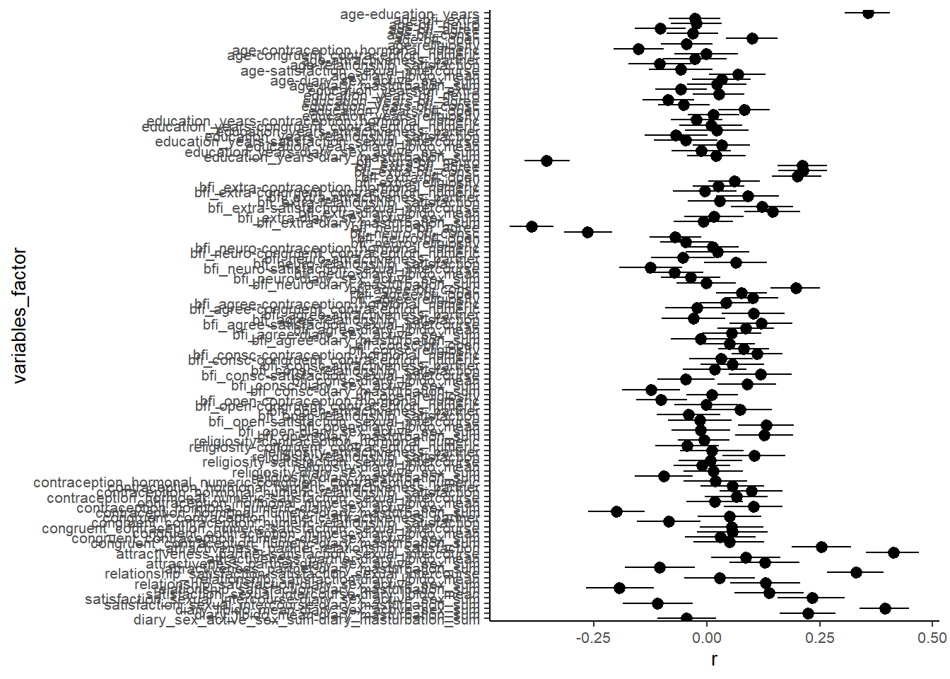
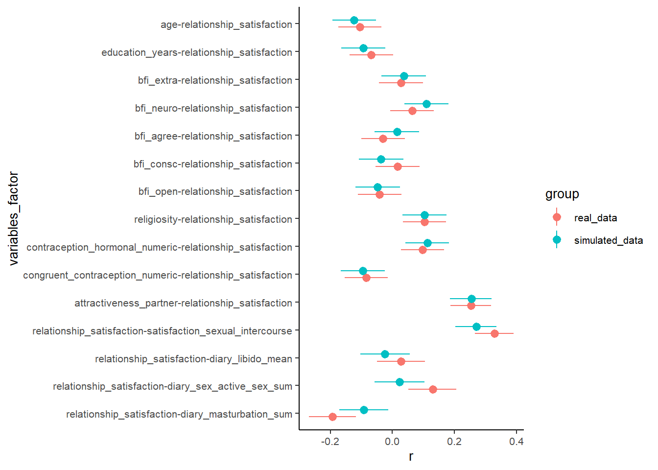
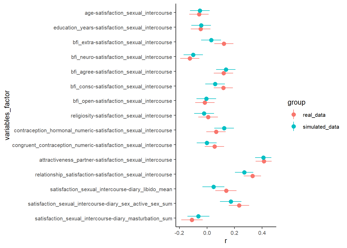
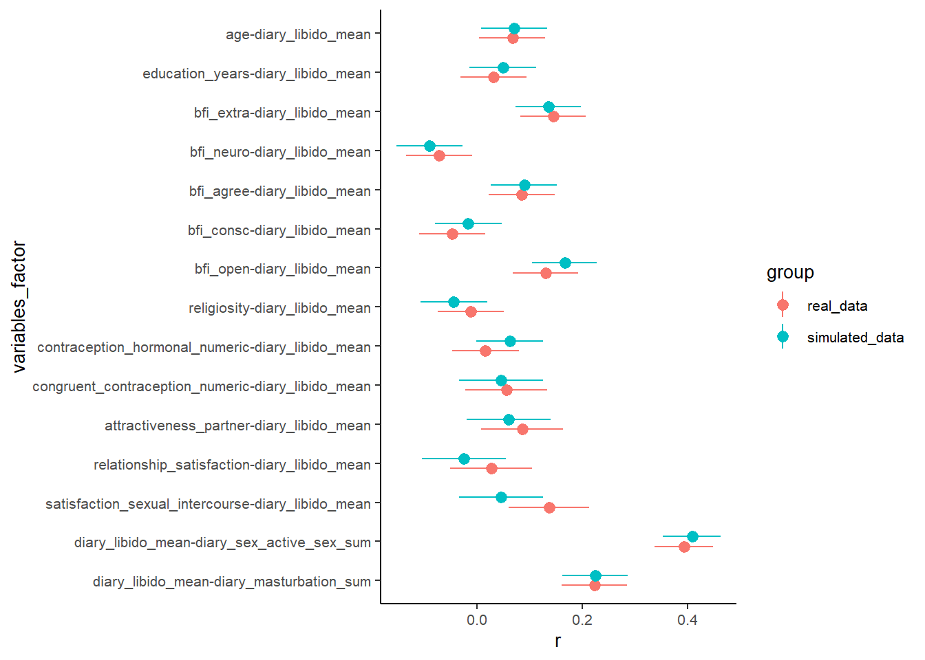
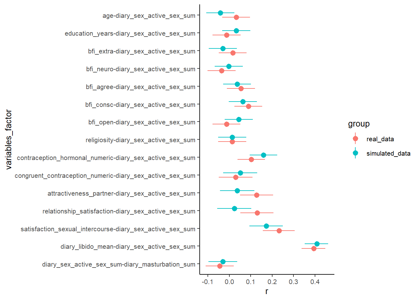
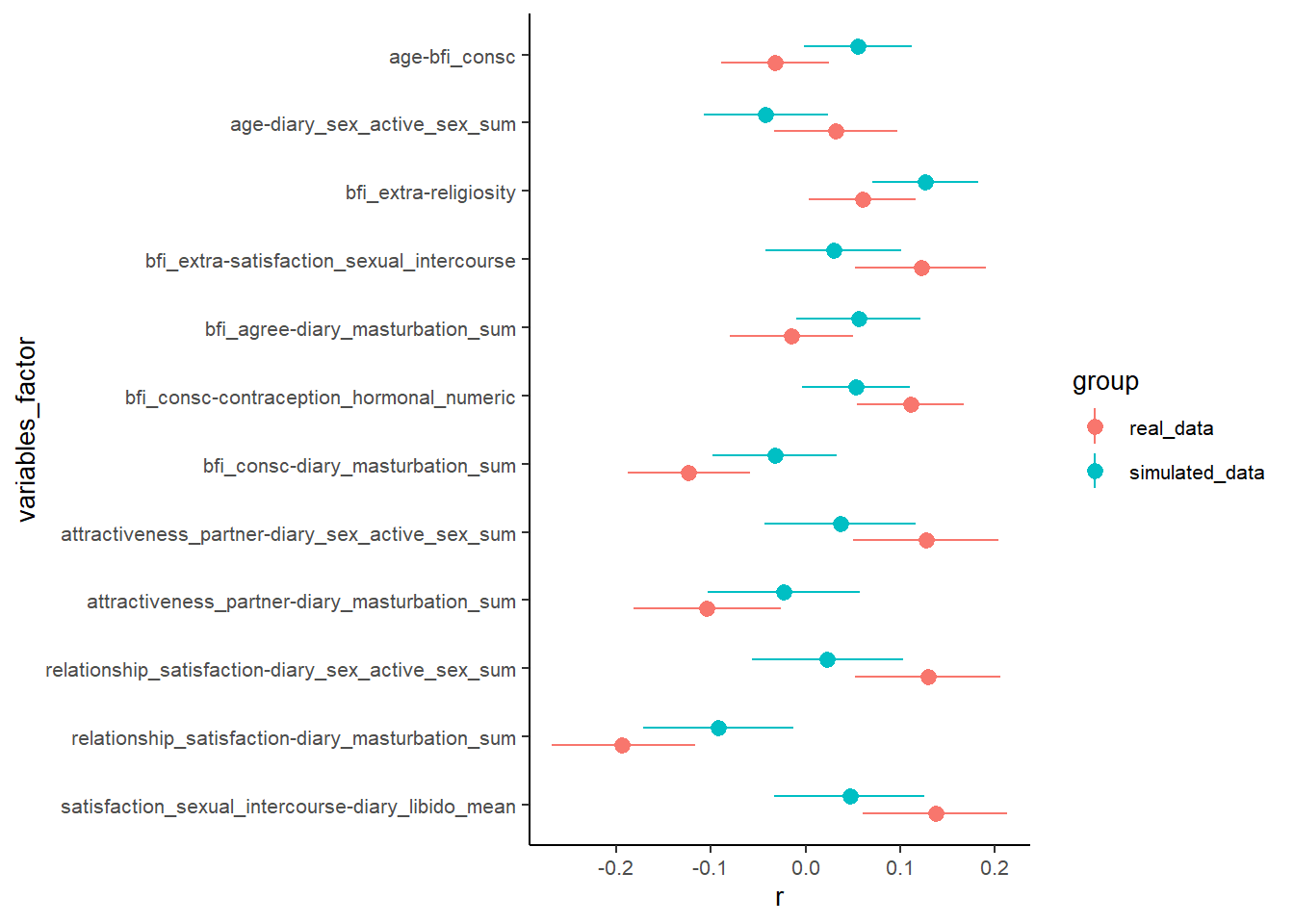
Main Analyses

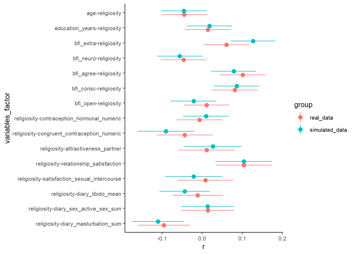
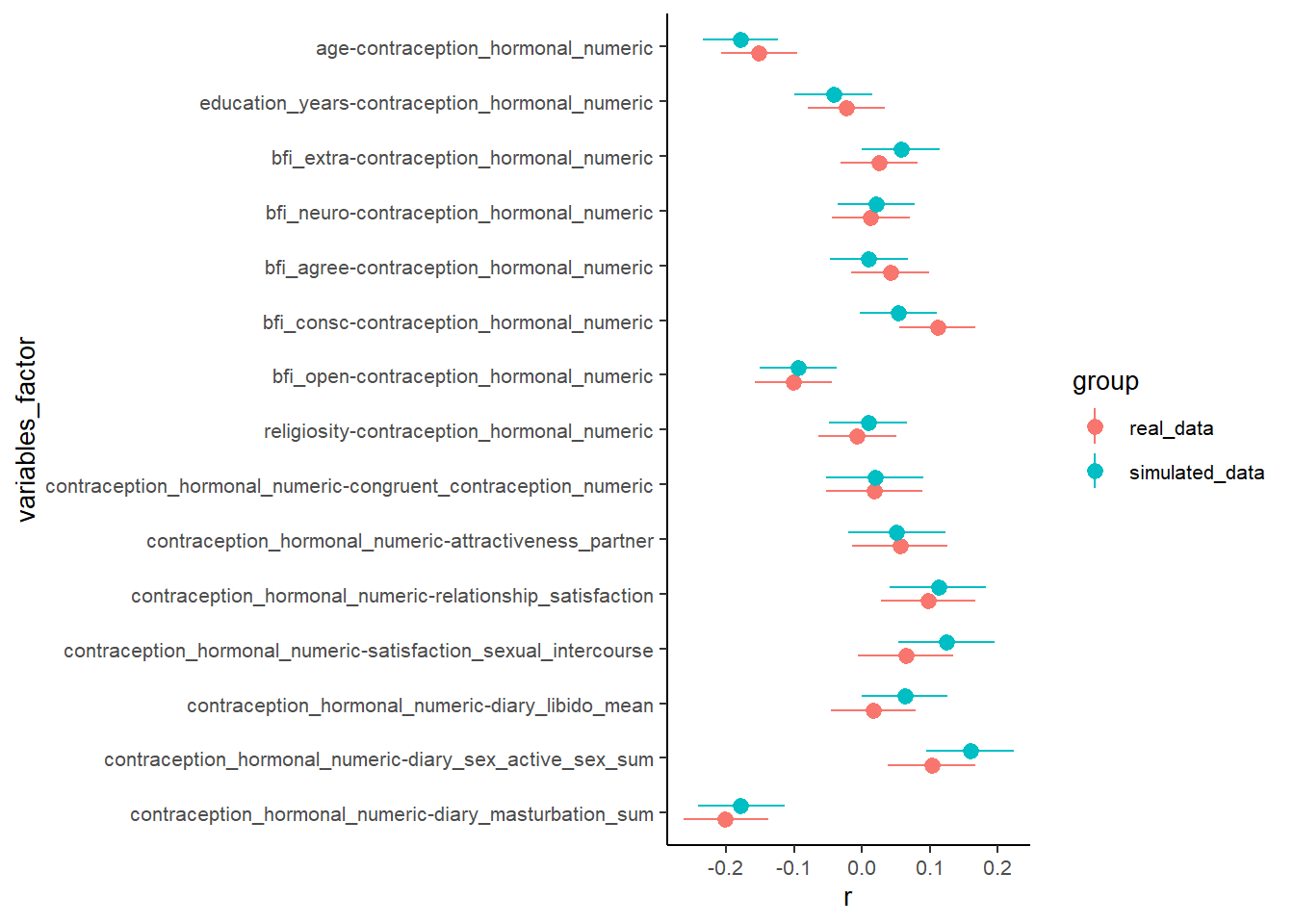
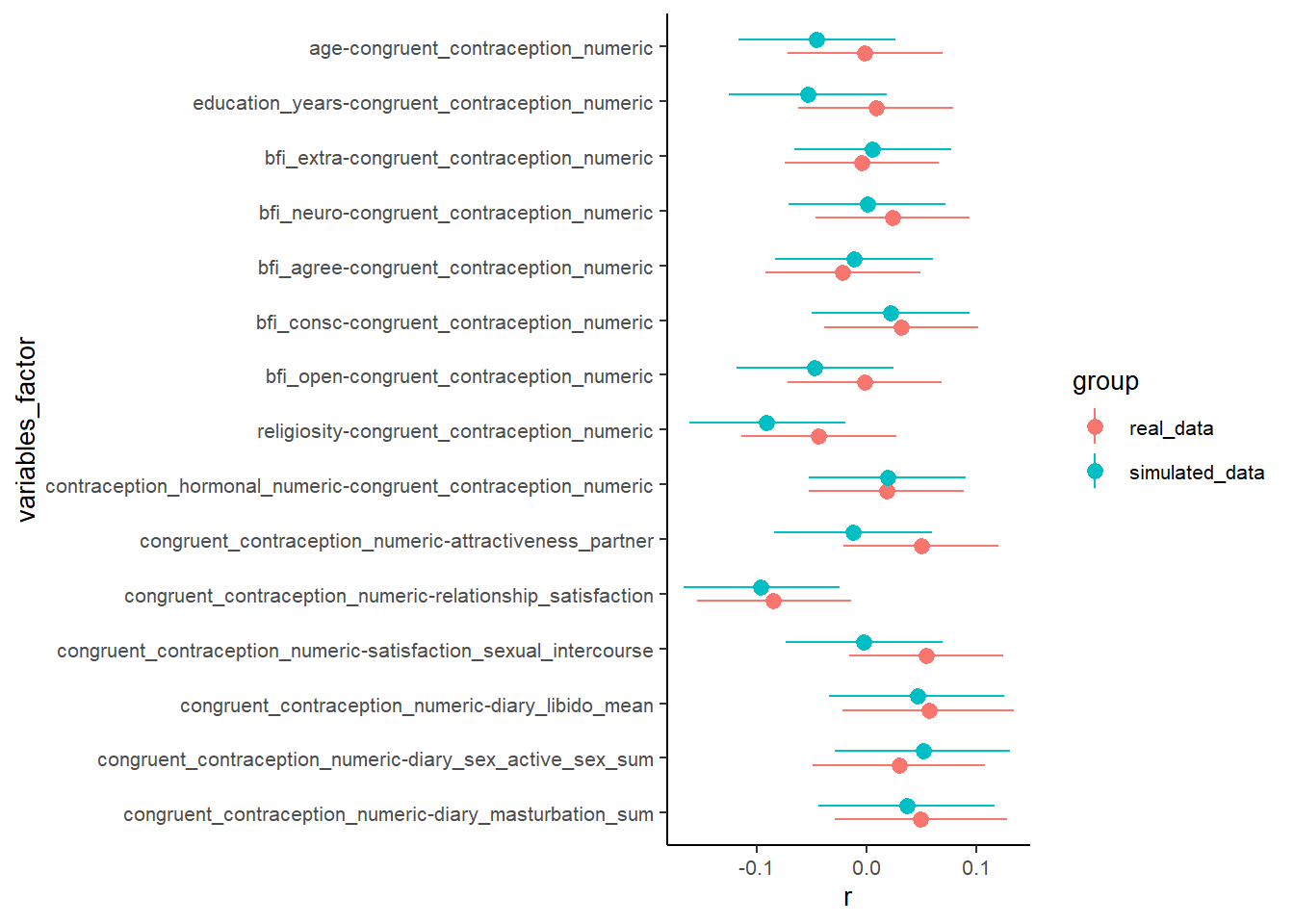
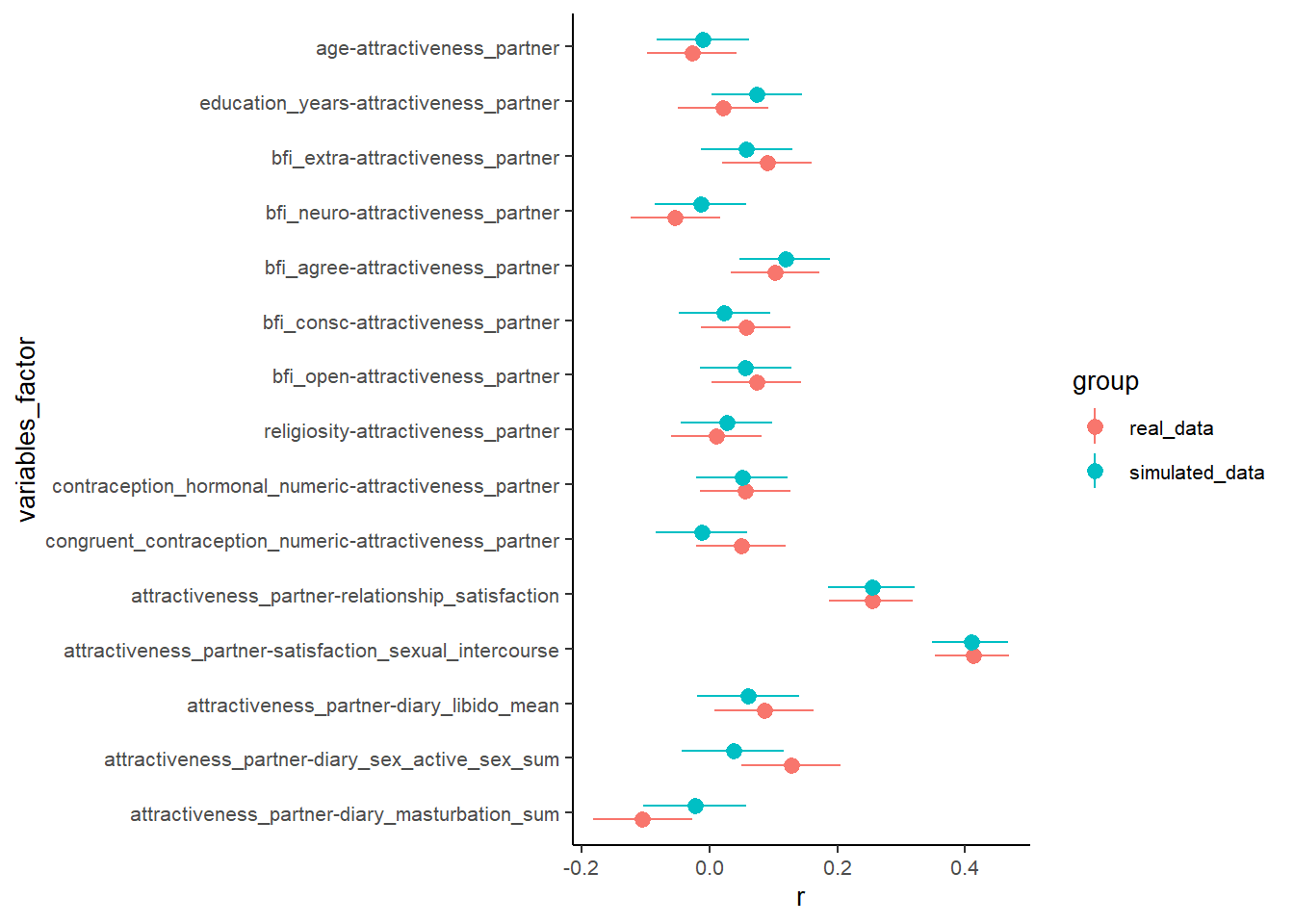
Selection effects

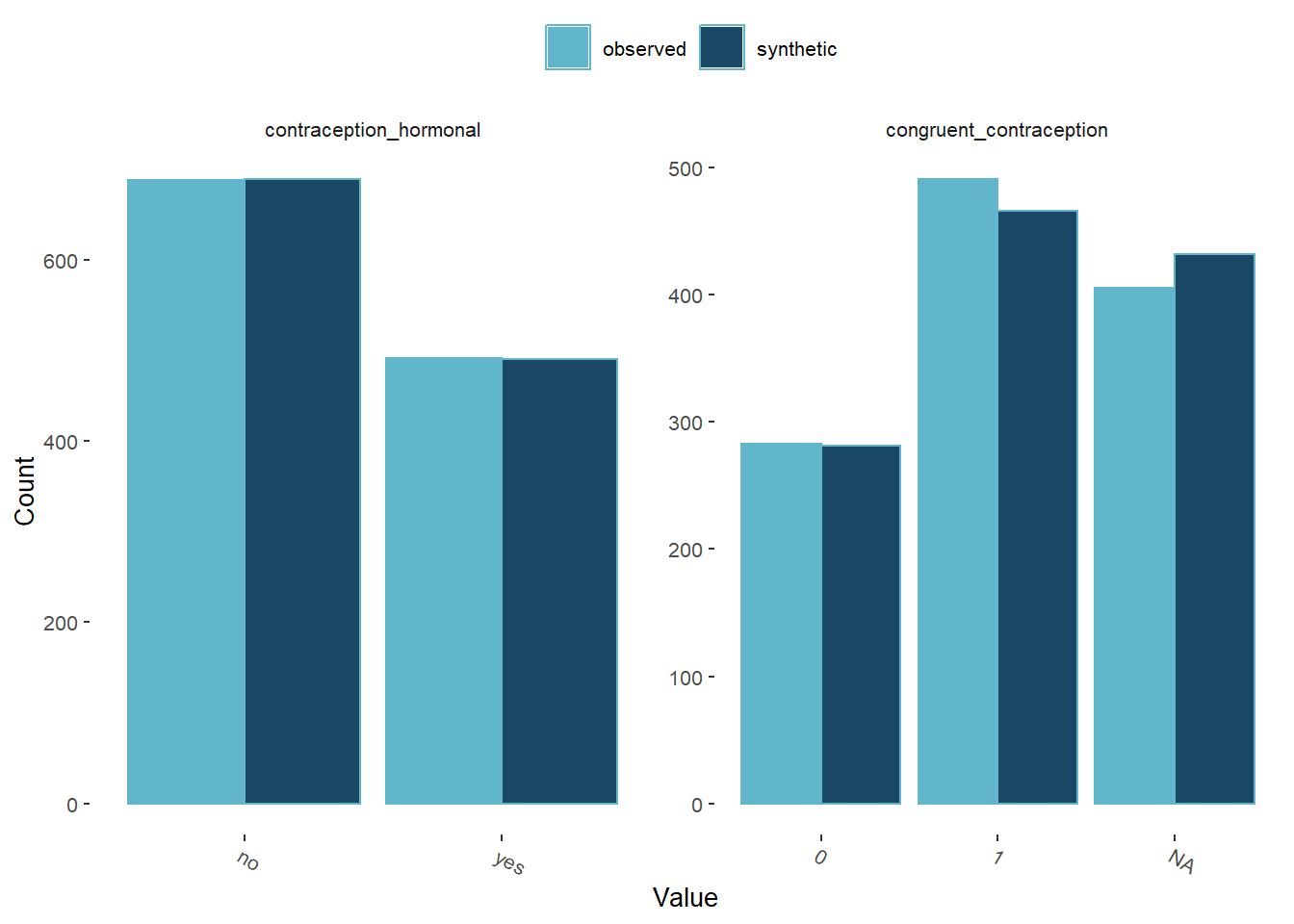
Hormonal Contraception

Simple Model

model = lm.synds(as.numeric(contraception_hormonal) ~
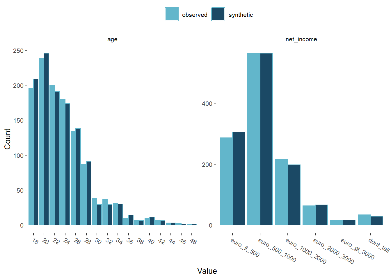
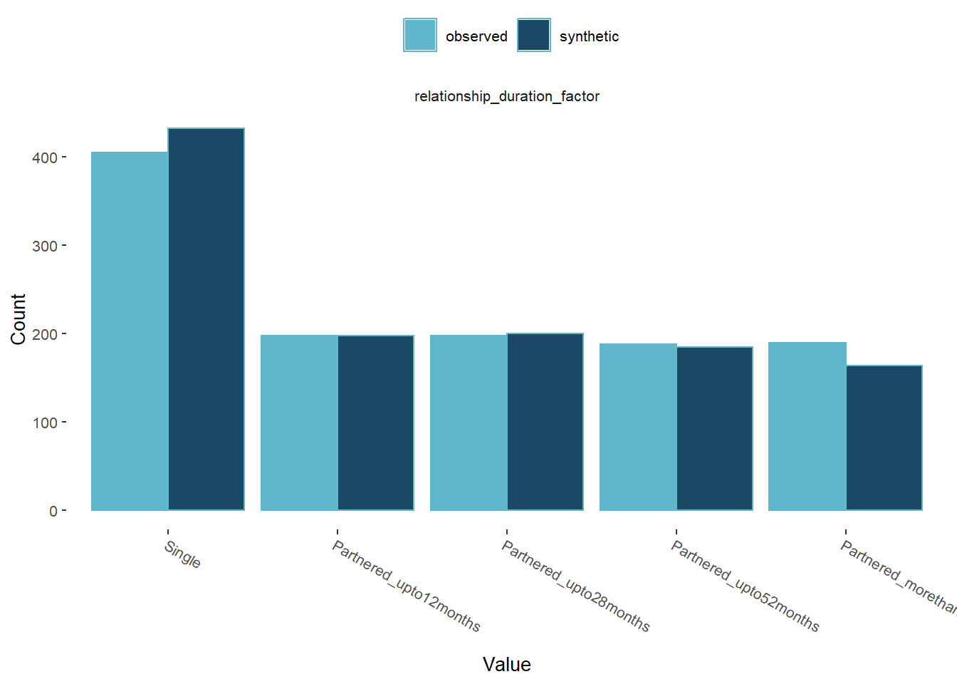
                   age + net_income + relationship_duration_factor,
                         data = example_sim)

t_test_com <- compare(
  model, # Results from the synthetic linear model
  data, # The original dataset
  lwd = 1.5, # The type of line in the plot
  lty = 1, # The width of line in the plot
  point.size = 4, # The size of the symbols used in the plot
  lcol = c("#62B6CB", "#1B4965") # Set the colours
)

t_test_com$ci.plot +
  ggtitle("") +
  apatheme +
  theme(text = element_text(size=10)) +
  background_grid()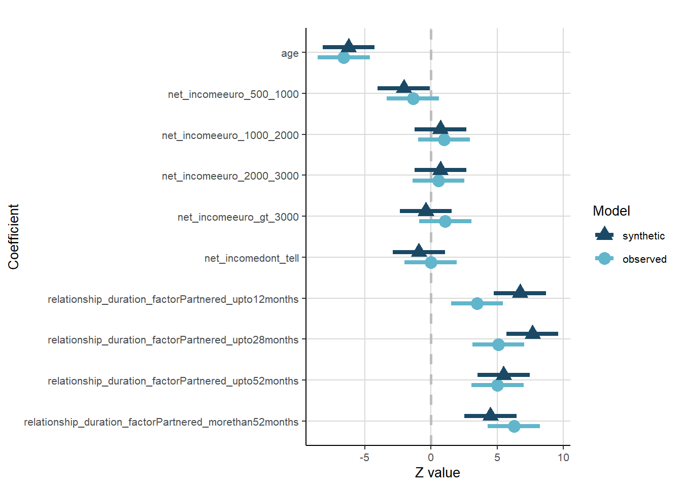

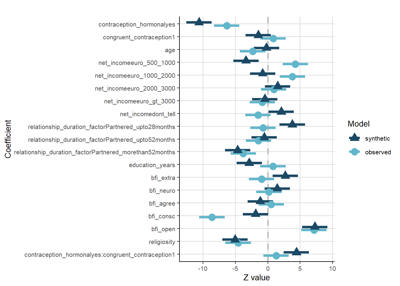
Complex Model

model = lm.synds(as.numeric(contraception_hormonal) ~
                   age + net_income + relationship_duration_factor +
                              education_years +
                              bfi_extra + bfi_neuro + bfi_agree + bfi_consc + bfi_open +
                              religiosity,
                         data = example_sim)

t_test_com <- compare(
  model, # Results from the synthetic linear model
  data, # The original dataset
  lwd = 1.5, # The type of line in the plot
  lty = 1, # The width of line in the plot
  point.size = 4, # The size of the symbols used in the plot
  lcol = c("#62B6CB", "#1B4965") # Set the colours
)

t_test_com$ci.plot +
  ggtitle("") +
  apatheme +
  theme(text = element_text(size=10)) +
  background_grid()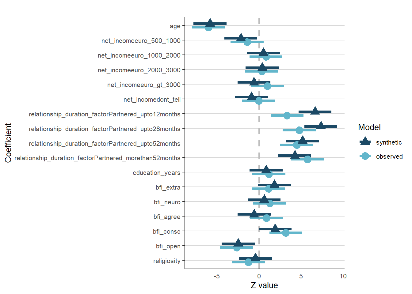

Congruent Use of Hormonal Contraception

Simple Model

model = lm.synds(as.numeric(congruent_contraception) ~
                   age + net_income + relationship_duration_factor,
                         data = example_sim)

t_test_com <- compare(
  model, # Results from the synthetic linear model
  data, # The original dataset
  lwd = 1.5, # The type of line in the plot
  lty = 1, # The width of line in the plot
  point.size = 4, # The size of the symbols used in the plot
  lcol = c("#62B6CB", "#1B4965") # Set the colours
)

t_test_com$ci.plot +
  ggtitle("") +
  apatheme +
  theme(text = element_text(size=10)) +
  background_grid()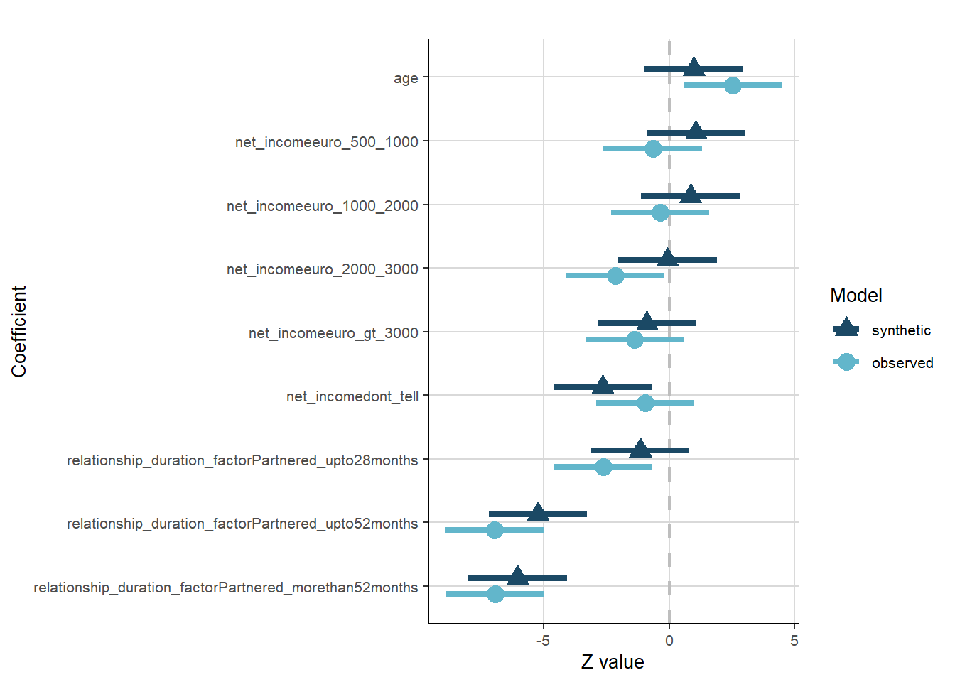

Complex Model

model = lm.synds(as.numeric(congruent_contraception) ~
                   age + net_income + relationship_duration_factor +
                              education_years +
                              bfi_extra + bfi_neuro + bfi_agree + bfi_consc + bfi_open +
                              religiosity,
                         data = example_sim)

t_test_com <- compare(
  model, # Results from the synthetic linear model
  data, # The original dataset
  lwd = 1.5, # The type of line in the plot
  lty = 1, # The width of line in the plot
  point.size = 4, # The size of the symbols used in the plot
  lcol = c("#62B6CB", "#1B4965") # Set the colours
)

t_test_com$ci.plot +
  ggtitle("") +
  apatheme +
  theme(text = element_text(size=10)) +
  background_grid()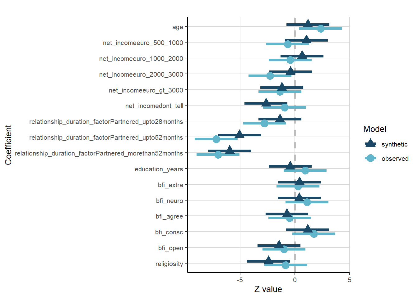

Effects of Hormonal Contraception

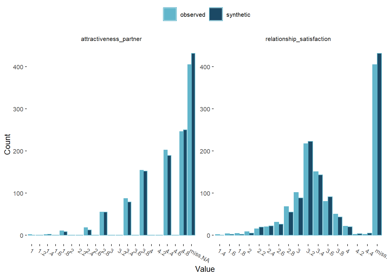
Attractiveness of Partner

Uncontrolled

model = lm.synds(attractiveness_partner ~ contraception_hormonal,
                         data = example_sim)

t_test_com <- compare(
  model, # Results from the synthetic linear model
  data, # The original dataset
  lwd = 1.5, # The type of line in the plot
  lty = 1, # The width of line in the plot
  point.size = 4, # The size of the symbols used in the plot
  lcol = c("#62B6CB", "#1B4965") # Set the colours
)

t_test_com$ci.plot +
  ggtitle("") +
  apatheme +
  theme(text = element_text(size=10)) +
  background_grid()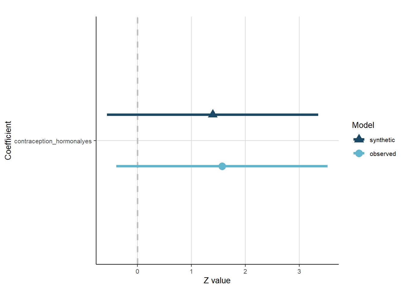

Controlled

model = lm.synds(attractiveness_partner ~ contraception_hormonal +
                        age + net_income + relationship_duration_factor +
                              education_years +
                              bfi_extra + bfi_neuro + bfi_agree + bfi_consc + bfi_open +
                              religiosity,
                         data = example_sim)

t_test_com <- compare(
  model, # Results from the synthetic linear model
  data, # The original dataset
  lwd = 1.5, # The type of line in the plot
  lty = 1, # The width of line in the plot
  point.size = 4, # The size of the symbols used in the plot
  lcol = c("#62B6CB", "#1B4965") # Set the colours
)

t_test_com$ci.plot +
  ggtitle("") +
  apatheme +
  theme(text = element_text(size=10)) +
  background_grid()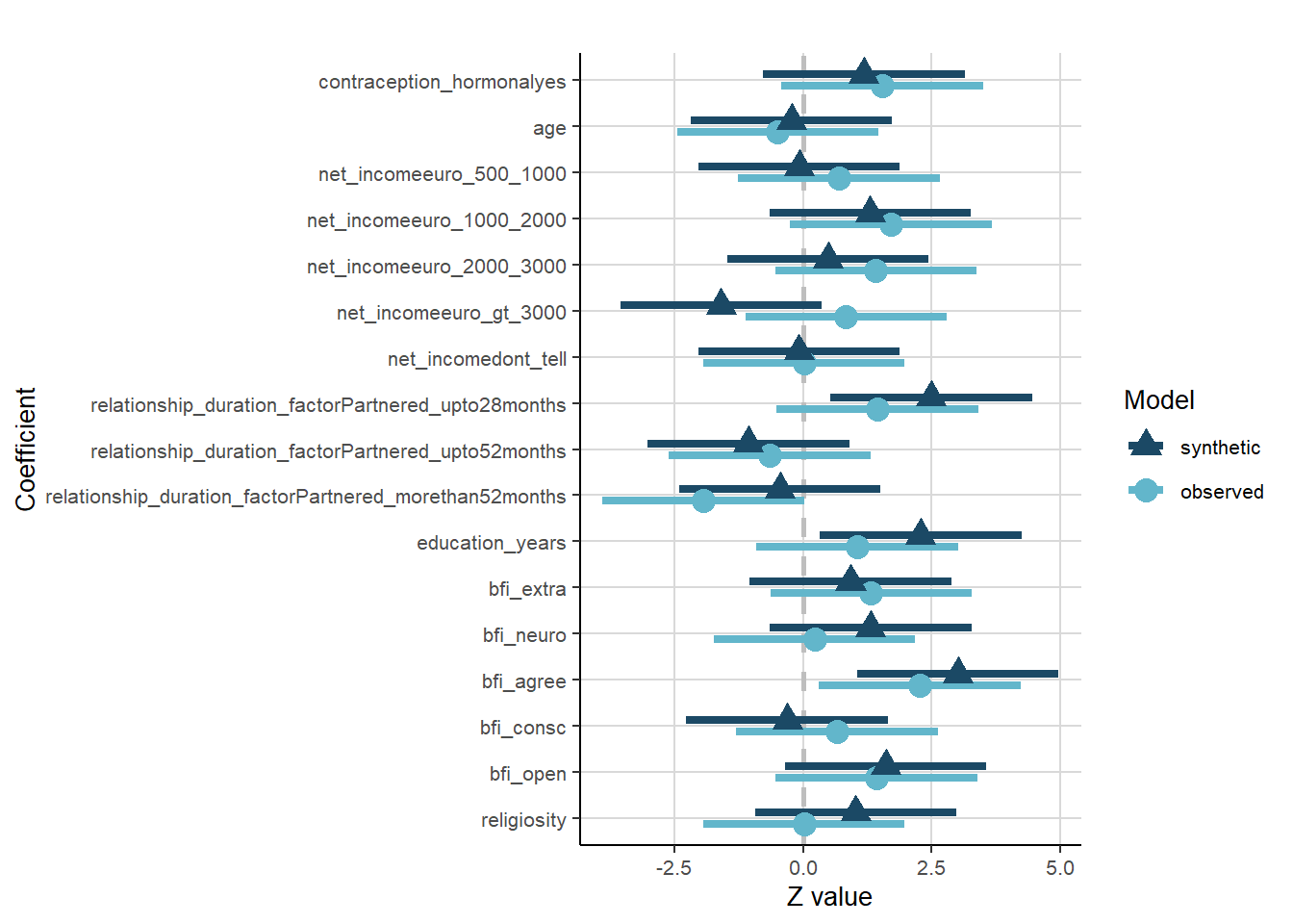

Relationship Satisfaction

Uncontrolled

model = lm.synds(relationship_satisfaction ~ contraception_hormonal,
                         data = example_sim)

t_test_com <- compare(
  model, # Results from the synthetic linear model
  data, # The original dataset
  lwd = 1.5, # The type of line in the plot
  lty = 1, # The width of line in the plot
  point.size = 4, # The size of the symbols used in the plot
  lcol = c("#62B6CB", "#1B4965") # Set the colours
)

t_test_com$ci.plot +
  ggtitle("") +
  apatheme +
  theme(text = element_text(size=10)) +
  background_grid()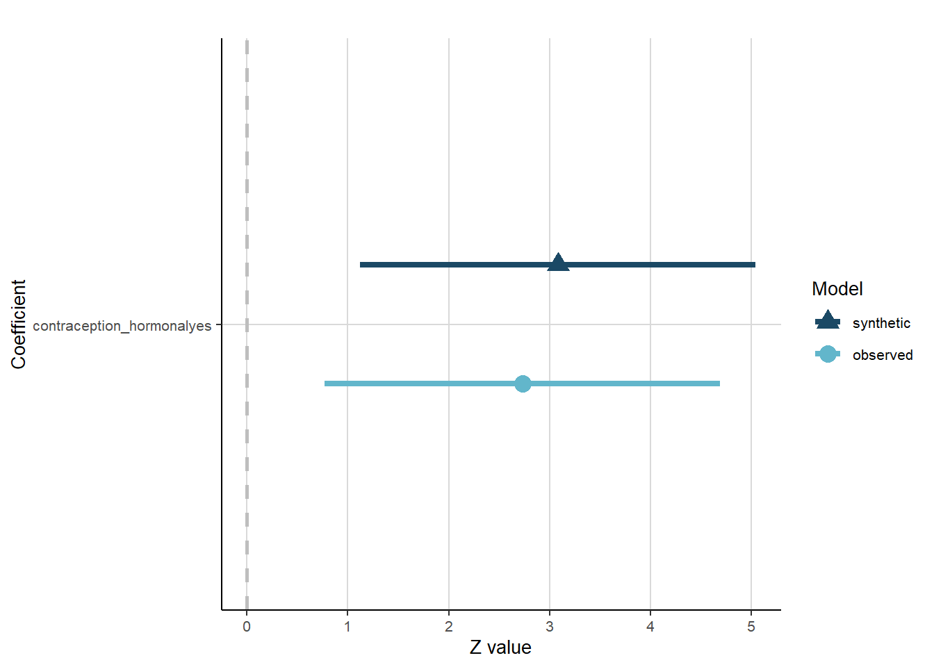

Controlled

model = lm.synds(relationship_satisfaction ~ contraception_hormonal +
                        age + net_income + relationship_duration_factor +
                              education_years +
                              bfi_extra + bfi_neuro + bfi_agree + bfi_consc + bfi_open +
                              religiosity,
                         data = example_sim)

t_test_com <- compare(
  model, # Results from the synthetic linear model
  data, # The original dataset
  lwd = 1.5, # The type of line in the plot
  lty = 1, # The width of line in the plot
  point.size = 4, # The size of the symbols used in the plot
  lcol = c("#62B6CB", "#1B4965") # Set the colours
)

t_test_com$ci.plot +
  ggtitle("") +
  apatheme +
  theme(text = element_text(size=10)) +
  background_grid()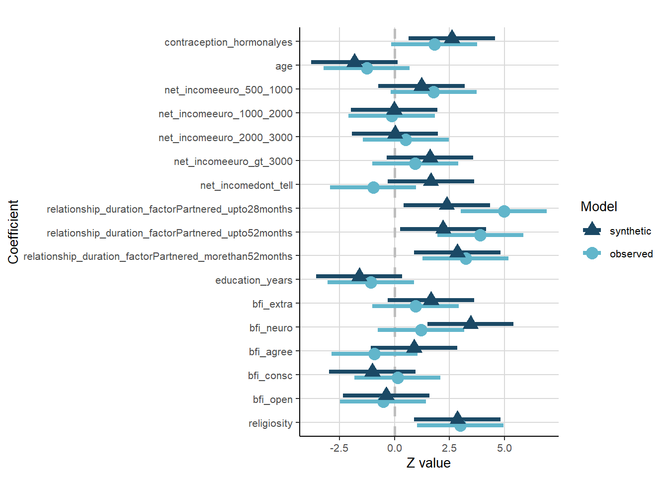

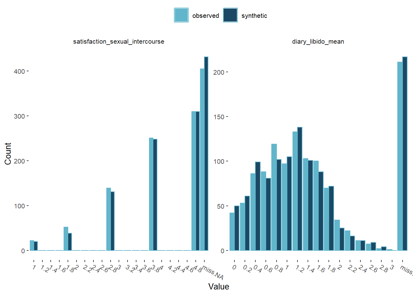
Sexual Satisfaction

Uncontrolled

model = lm.synds(satisfaction_sexual_intercourse ~ contraception_hormonal,
                         data = example_sim)

t_test_com <- compare(
  model, # Results from the synthetic linear model
  data, # The original dataset
  lwd = 1.5, # The type of line in the plot
  lty = 1, # The width of line in the plot
  point.size = 4, # The size of the symbols used in the plot
  lcol = c("#62B6CB", "#1B4965") # Set the colours
)

t_test_com$ci.plot +
  ggtitle("") +
  apatheme +
  theme(text = element_text(size=10)) +
  background_grid()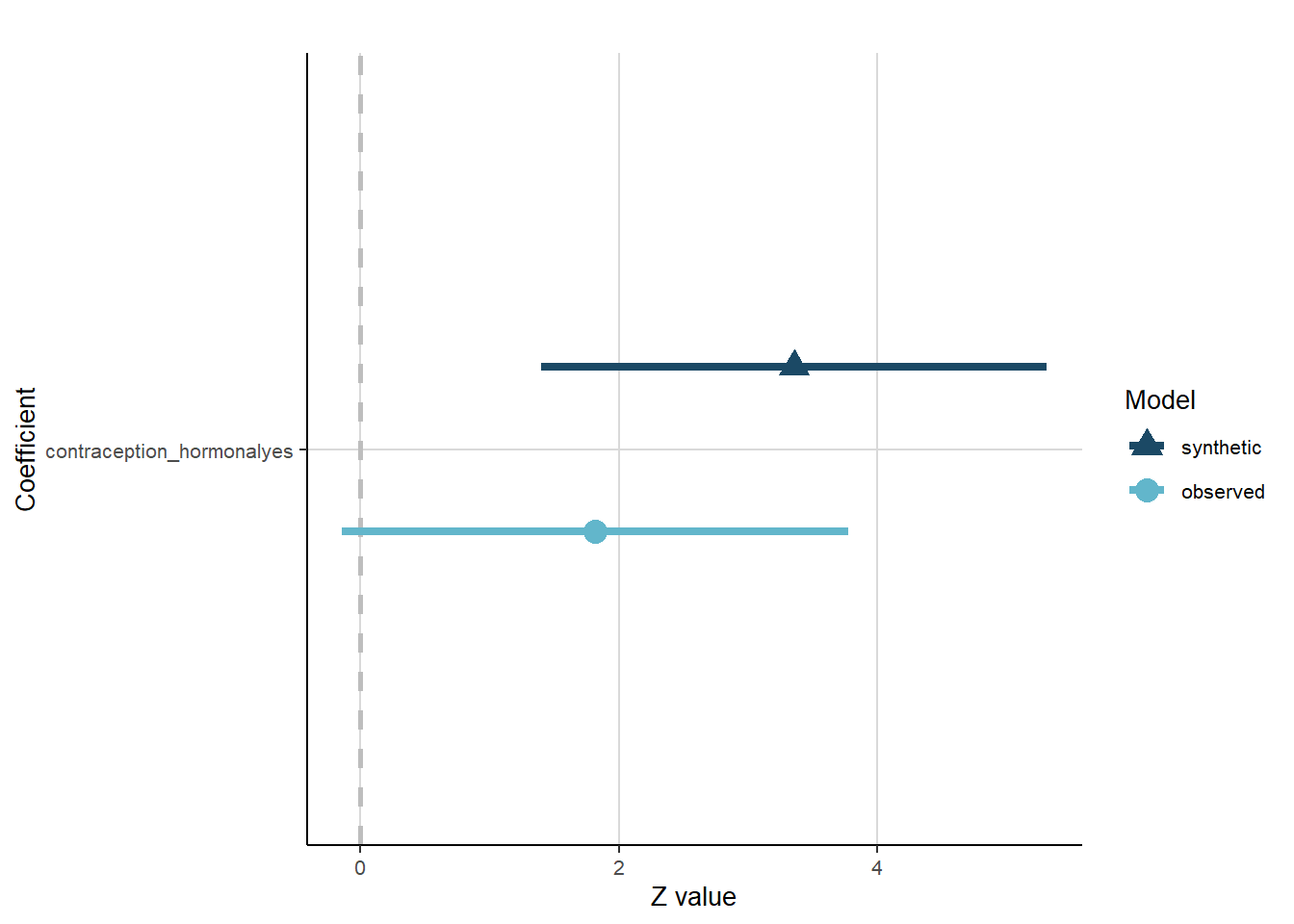

Controlled

model = lm.synds(satisfaction_sexual_intercourse ~ contraception_hormonal +
                        age + net_income + relationship_duration_factor +
                              education_years +
                              bfi_extra + bfi_neuro + bfi_agree + bfi_consc + bfi_open +
                              religiosity,
                         data = example_sim)

t_test_com <- compare(
  model, # Results from the synthetic linear model
  data, # The original dataset
  lwd = 1.5, # The type of line in the plot
  lty = 1, # The width of line in the plot
  point.size = 4, # The size of the symbols used in the plot
  lcol = c("#62B6CB", "#1B4965") # Set the colours
)

t_test_com$ci.plot +
  ggtitle("") +
  apatheme +
  theme(text = element_text(size=10)) +
  background_grid()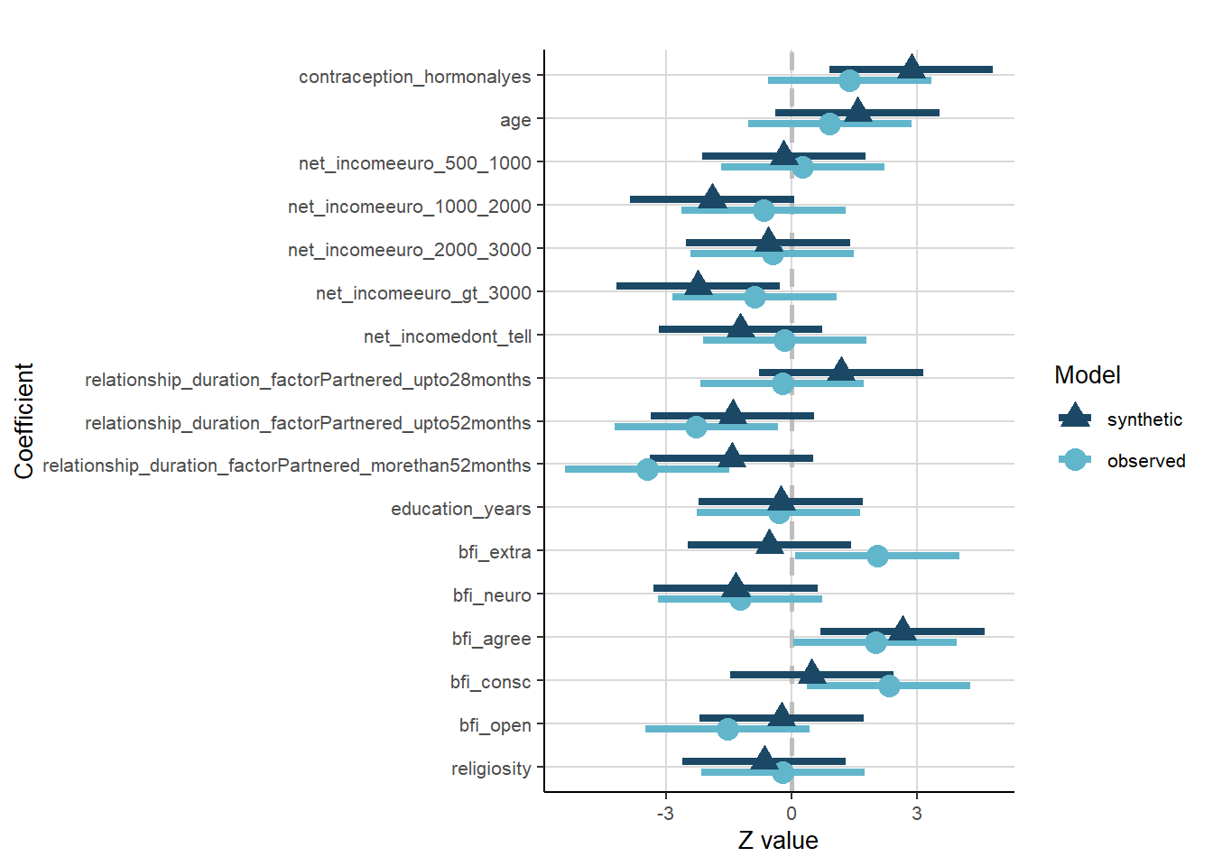

Libido

Uncontrolled

model = lm.synds(diary_libido_mean ~ contraception_hormonal,
                         data = example_sim)

t_test_com <- compare(
  model, # Results from the synthetic linear model
  data, # The original dataset
  lwd = 1.5, # The type of line in the plot
  lty = 1, # The width of line in the plot
  point.size = 4, # The size of the symbols used in the plot
  lcol = c("#62B6CB", "#1B4965") # Set the colours
)

t_test_com$ci.plot +
  ggtitle("") +
  apatheme +
  theme(text = element_text(size=10)) +
  background_grid()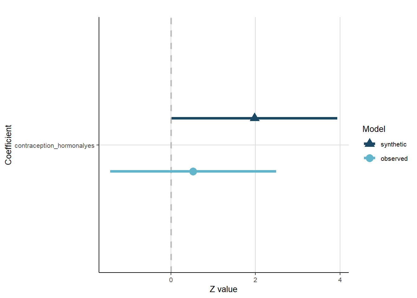

Controlled

model = lm.synds(diary_libido_mean ~ contraception_hormonal +
                        age + net_income + relationship_duration_factor +
                              education_years +
                              bfi_extra + bfi_neuro + bfi_agree + bfi_consc + bfi_open +
                              religiosity,
                         data = example_sim)

t_test_com <- compare(
  model, # Results from the synthetic linear model
  data, # The original dataset
  lwd = 1.5, # The type of line in the plot
  lty = 1, # The width of line in the plot
  point.size = 4, # The size of the symbols used in the plot
  lcol = c("#62B6CB", "#1B4965") # Set the colours
)

t_test_com$ci.plot +
  ggtitle("") +
  apatheme +
  theme(text = element_text(size=10)) +
  background_grid()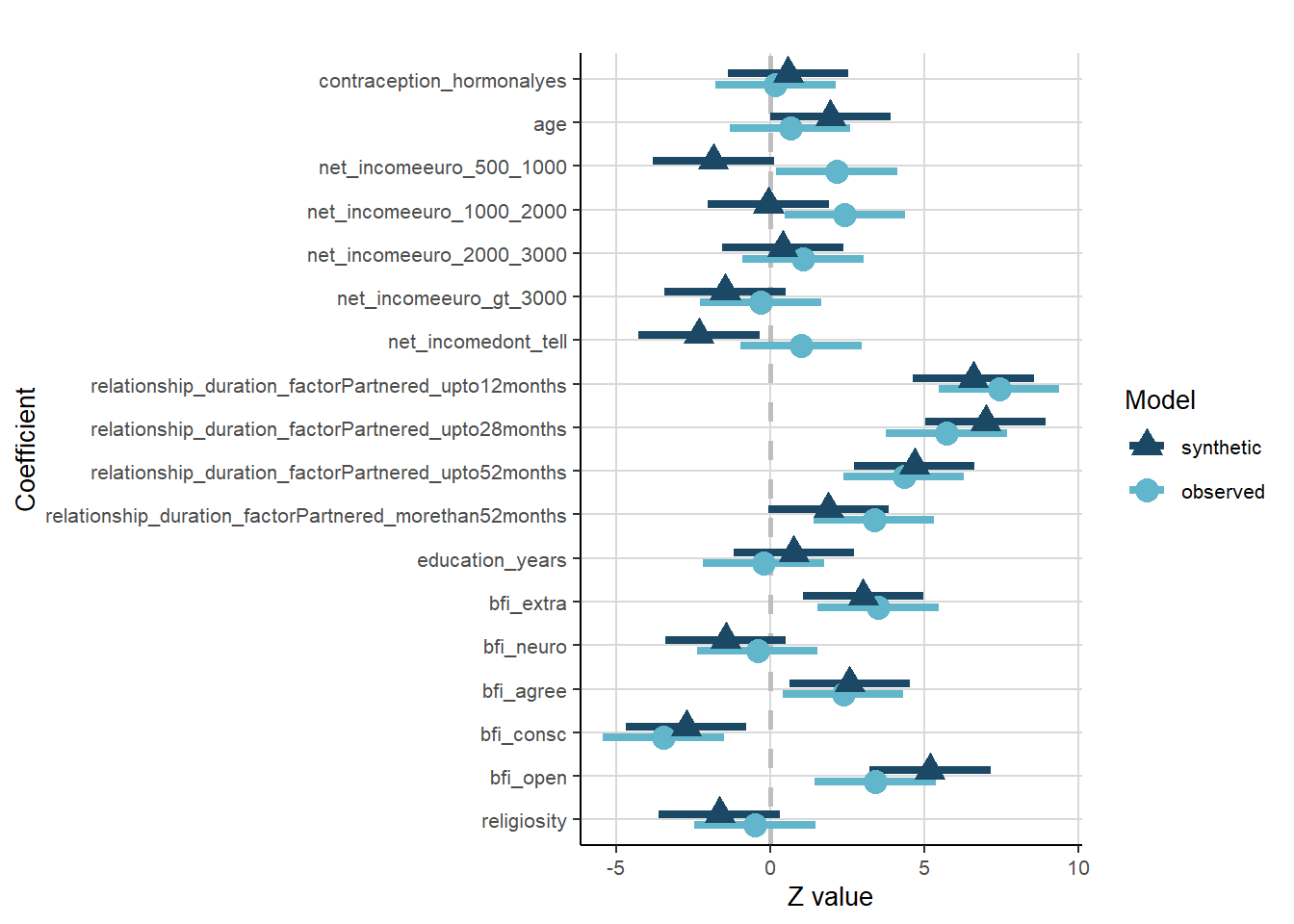

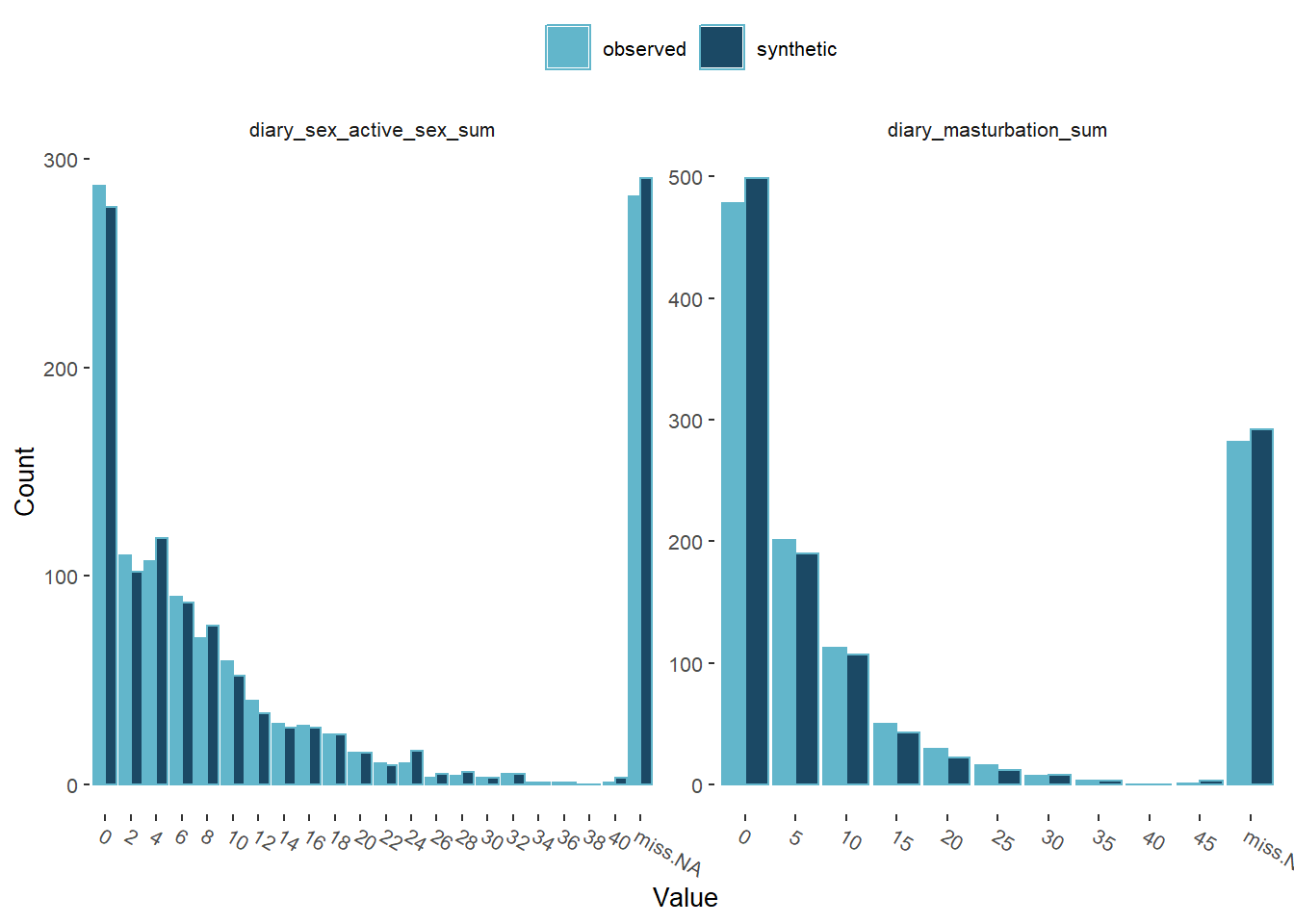
Sexual Frequency

Uncontrolled

model = glm.synds(diary_sex_active_sex_sum ~ offset(log(number_of_days)) +
                        contraception_hormonal,
                         data = example_sim, family = "poisson")

t_test_com <- compare(
  model, # Results from the synthetic linear model
  data, # The original dataset
  lwd = 1.5, # The type of line in the plot
  lty = 1, # The width of line in the plot
  point.size = 4, # The size of the symbols used in the plot
  lcol = c("#62B6CB", "#1B4965") # Set the colours
)

t_test_com$ci.plot +
  ggtitle("") +
  apatheme +
  theme(text = element_text(size=10)) +
  background_grid()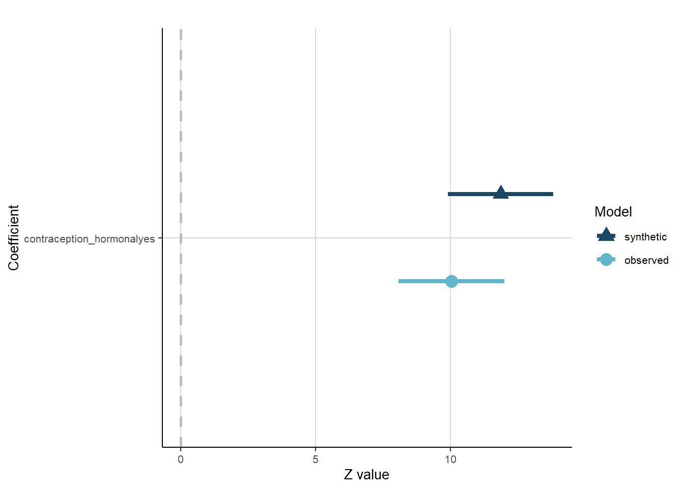

Controlled

model = glm.synds(diary_sex_active_sex_sum ~ offset(log(number_of_days)) +
                        contraception_hormonal +
                        age + net_income + relationship_duration_factor +
                              education_years +
                              bfi_extra + bfi_neuro + bfi_agree + bfi_consc + bfi_open +
                              religiosity,
                         data = example_sim, family = "poisson")

t_test_com <- compare(
  model, # Results from the synthetic linear model
  data, # The original dataset
  lwd = 1.5, # The type of line in the plot
  lty = 1, # The width of line in the plot
  point.size = 4, # The size of the symbols used in the plot
  lcol = c("#62B6CB", "#1B4965") # Set the colours
)

t_test_com$ci.plot +
  ggtitle("") +
  apatheme +
  theme(text = element_text(size=10)) +
  background_grid()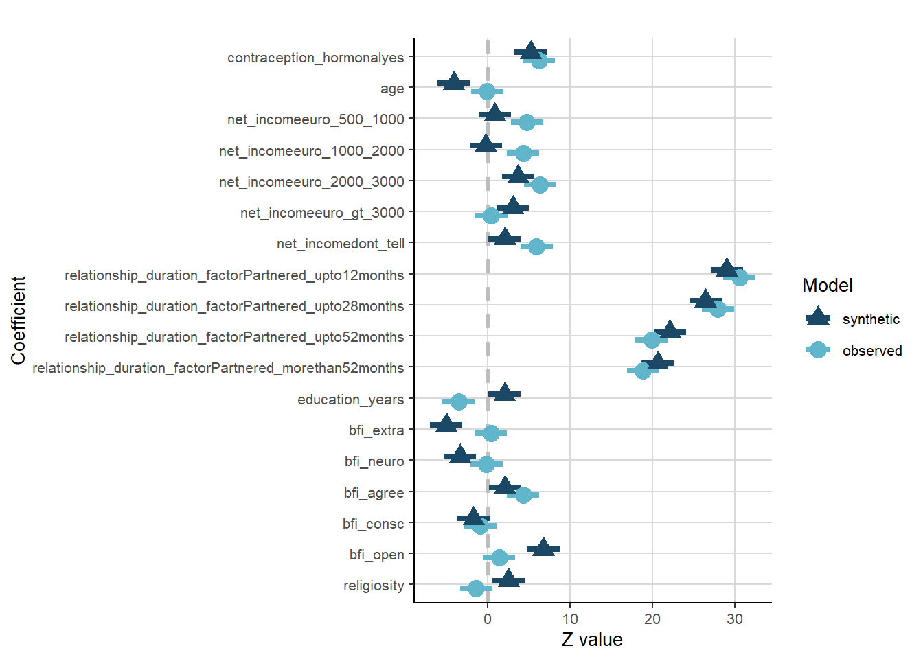

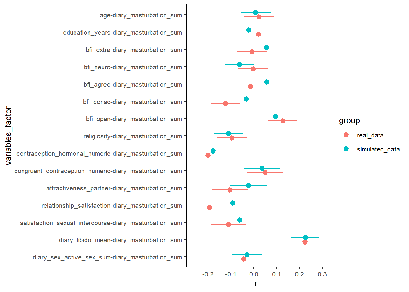
Masturbation Frequency

Uncontrolled

model = glm.synds(diary_masturbation_sum ~ offset(log(number_of_days)) +
                        contraception_hormonal,
                         data = example_sim, family = "poisson")

t_test_com <- compare(
  model, # Results from the synthetic linear model
  data, # The original dataset
  lwd = 1.5, # The type of line in the plot
  lty = 1, # The width of line in the plot
  point.size = 4, # The size of the symbols used in the plot
  lcol = c("#62B6CB", "#1B4965") # Set the colours
)

t_test_com$ci.plot +
  ggtitle("") +
  apatheme +
  theme(text = element_text(size=10)) +
  background_grid()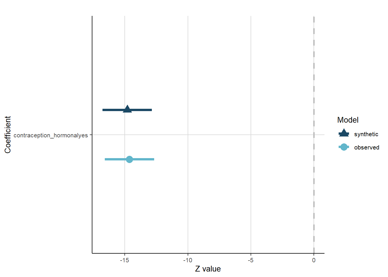

Controlled

model = glm.synds(diary_masturbation_sum ~ offset(log(number_of_days)) +
                        contraception_hormonal +
                        age + net_income + relationship_duration_factor +
                              education_years +
                              bfi_extra + bfi_neuro + bfi_agree + bfi_consc + bfi_open +
                              religiosity,
                         data = example_sim, family = "poisson")

t_test_com <- compare(
  model, # Results from the synthetic linear model
  data, # The original dataset
  lwd = 1.5, # The type of line in the plot
  lty = 1, # The width of line in the plot
  point.size = 4, # The size of the symbols used in the plot
  lcol = c("#62B6CB", "#1B4965") # Set the colours
)

t_test_com$ci.plot +
  ggtitle("") +
  apatheme +
  theme(text = element_text(size=10)) +
  background_grid()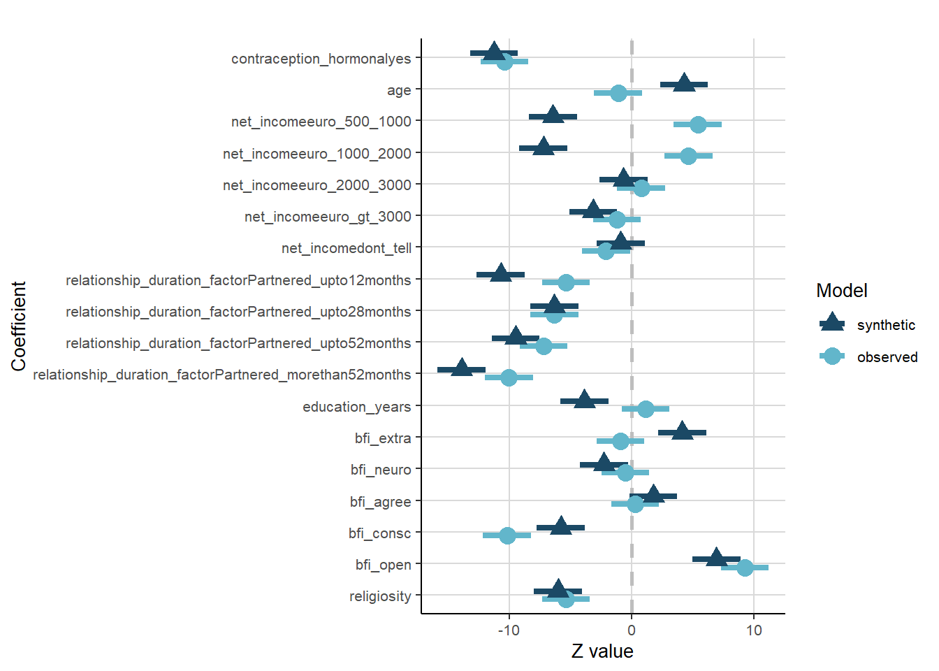

HC, Congruent Use of HC and Their Interaction

Attractiveness of Partner

Uncontrolled

model = lm.synds(attractiveness_partner ~ contraception_hormonal * congruent_contraception,
                 data = example_sim)

t_test_com <- compare(
  model, # Results from the synthetic linear model
  data, # The original dataset
  lwd = 1.5, # The type of line in the plot
  lty = 1, # The width of line in the plot
  point.size = 4, # The size of the symbols used in the plot
  lcol = c("#62B6CB", "#1B4965") # Set the colours
)

t_test_com$ci.plot +
  ggtitle("") +
  apatheme +
  theme(text = element_text(size=10)) +
  background_grid()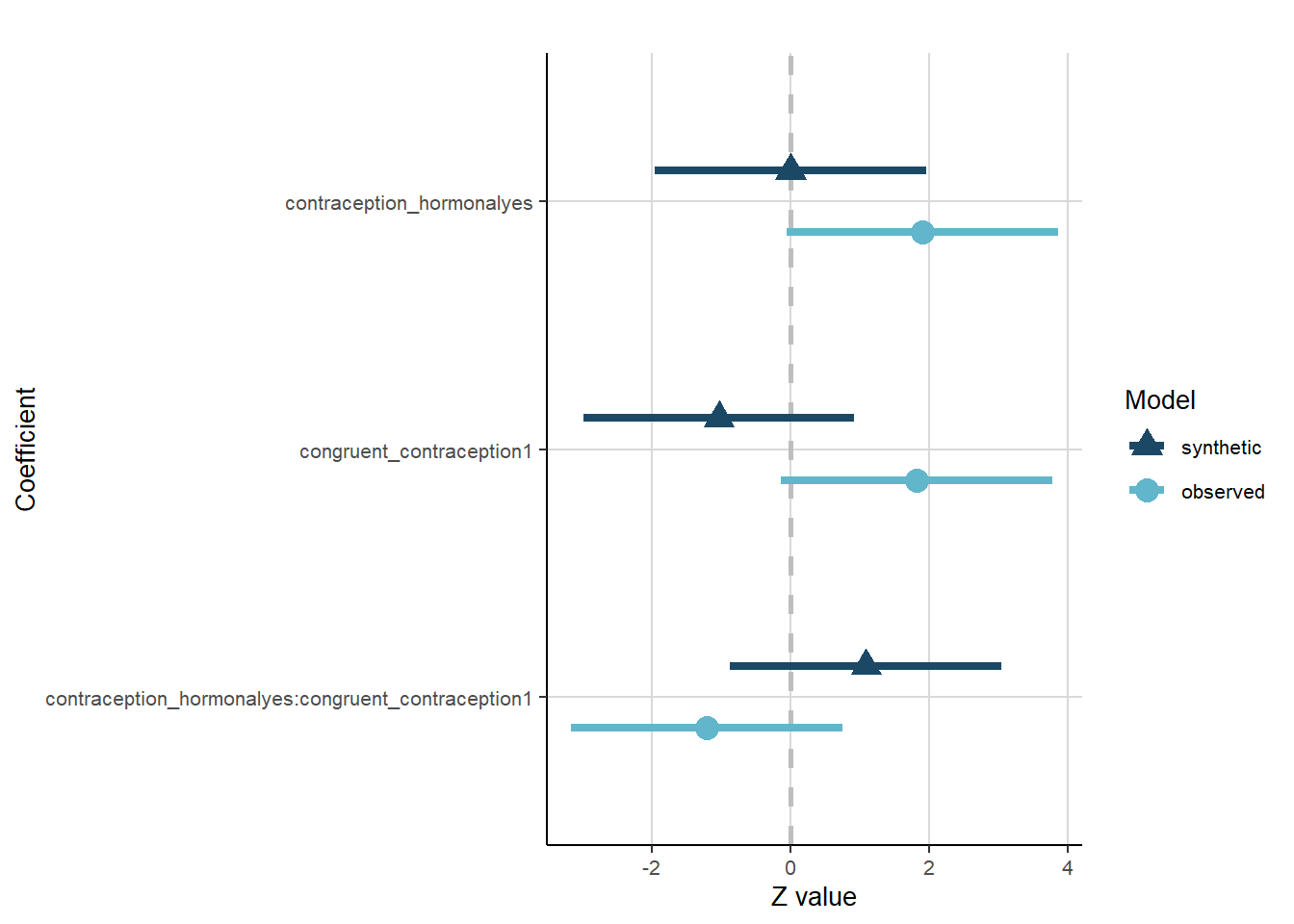

Controlled

model = lm.synds(attractiveness_partner ~ contraception_hormonal * congruent_contraception +
                   age + net_income + relationship_duration_factor +
                   education_years +
                   bfi_extra + bfi_neuro + bfi_agree + bfi_consc + bfi_open +
                   religiosity,
                 data = example_sim)

t_test_com <- compare(
  model, # Results from the synthetic linear model
  data, # The original dataset
  lwd = 1.5, # The type of line in the plot
  lty = 1, # The width of line in the plot
  point.size = 4, # The size of the symbols used in the plot
  lcol = c("#62B6CB", "#1B4965") # Set the colours
)

t_test_com$ci.plot +
  ggtitle("") +
  apatheme +
  theme(text = element_text(size=10)) +
  background_grid()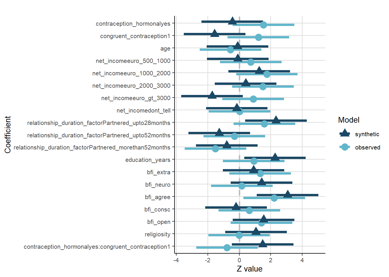

Relationship Satisfaction

Uncontrolled

model = lm.synds(relationship_satisfaction ~ contraception_hormonal * congruent_contraception,
                 data = example_sim)

t_test_com <- compare(
  model, # Results from the synthetic linear model
  data, # The original dataset
  lwd = 1.5, # The type of line in the plot
  lty = 1, # The width of line in the plot
  point.size = 4, # The size of the symbols used in the plot
  lcol = c("#62B6CB", "#1B4965") # Set the colours
)

t_test_com$ci.plot +
  ggtitle("") +
  apatheme +
  theme(text = element_text(size=10)) +
  background_grid()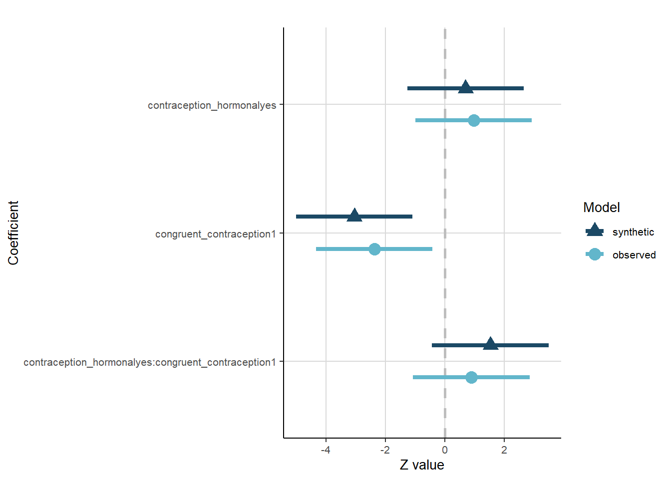

Controlled

model = lm.synds(relationship_satisfaction ~ contraception_hormonal * congruent_contraception +
                   age + net_income + relationship_duration_factor +
                   education_years +
                   bfi_extra + bfi_neuro + bfi_agree + bfi_consc + bfi_open +
                   religiosity,
                 data = example_sim)

t_test_com <- compare(
  model, # Results from the synthetic linear model
  data, # The original dataset
  lwd = 1.5, # The type of line in the plot
  lty = 1, # The width of line in the plot
  point.size = 4, # The size of the symbols used in the plot
  lcol = c("#62B6CB", "#1B4965") # Set the colours
)

t_test_com$ci.plot +
  ggtitle("") +
  apatheme +
  theme(text = element_text(size=10)) +
  background_grid()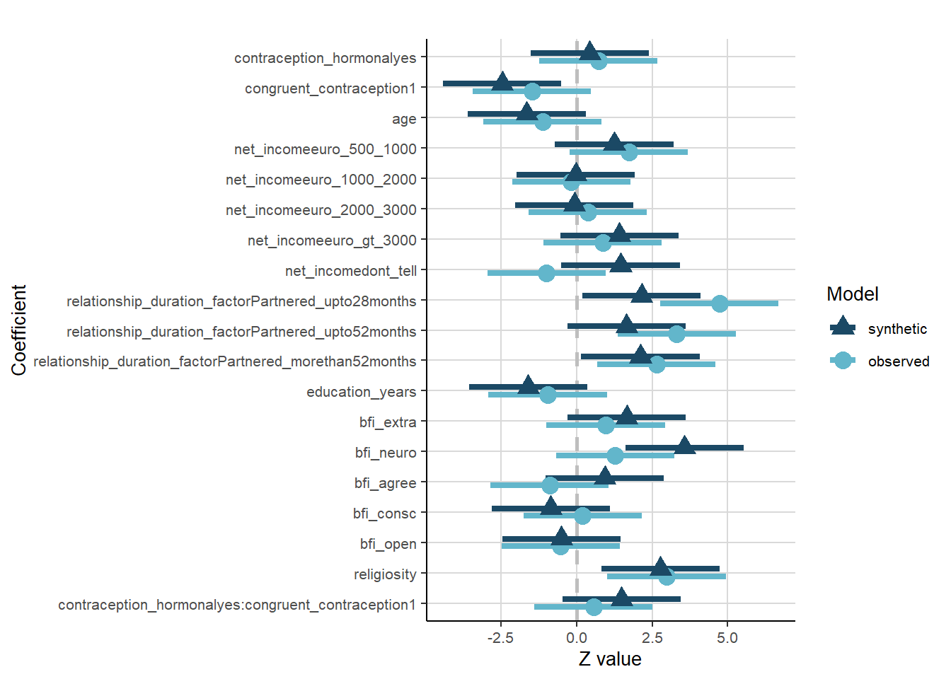

Sexual Satisfaction

Uncontrolled

model = lm.synds(satisfaction_sexual_intercourse ~ contraception_hormonal * congruent_contraception,
                 data = example_sim)

t_test_com <- compare(
  model, # Results from the synthetic linear model
  data, # The original dataset
  lwd = 1.5, # The type of line in the plot
  lty = 1, # The width of line in the plot
  point.size = 4, # The size of the symbols used in the plot
  lcol = c("#62B6CB", "#1B4965") # Set the colours
)

t_test_com$ci.plot +
  ggtitle("") +
  apatheme +
  theme(text = element_text(size=10)) +
  background_grid()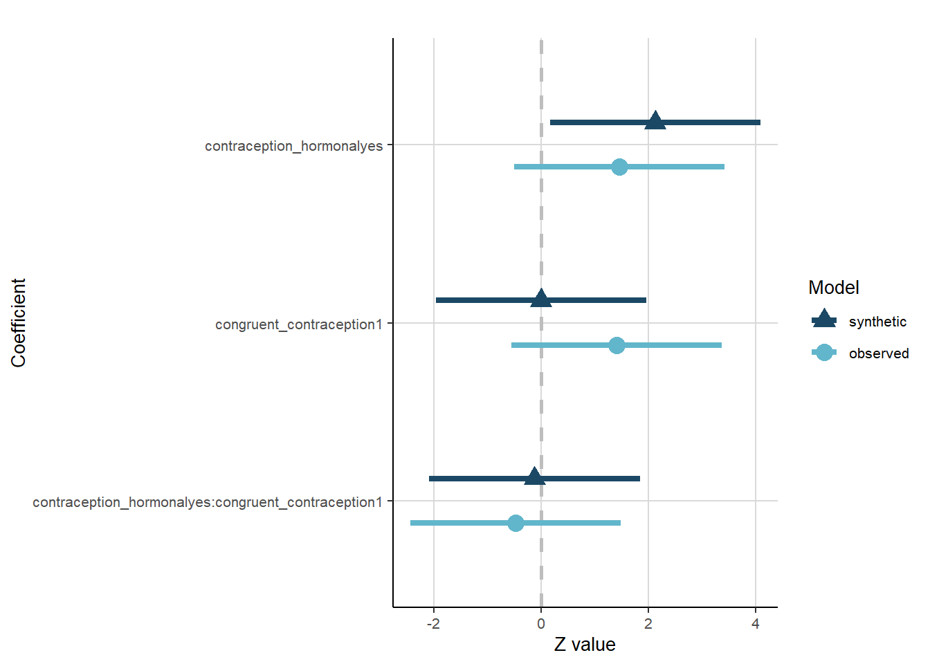

Controlled

model = lm.synds(satisfaction_sexual_intercourse ~ contraception_hormonal * congruent_contraception +
                   age + net_income + relationship_duration_factor +
                   education_years +
                   bfi_extra + bfi_neuro + bfi_agree + bfi_consc + bfi_open +
                   religiosity,
                 data = example_sim)

t_test_com <- compare(
  model, # Results from the synthetic linear model
  data, # The original dataset
  lwd = 1.5, # The type of line in the plot
  lty = 1, # The width of line in the plot
  point.size = 4, # The size of the symbols used in the plot
  lcol = c("#62B6CB", "#1B4965") # Set the colours
)

t_test_com$ci.plot +
  ggtitle("") +
  apatheme +
  theme(text = element_text(size=10)) +
  background_grid()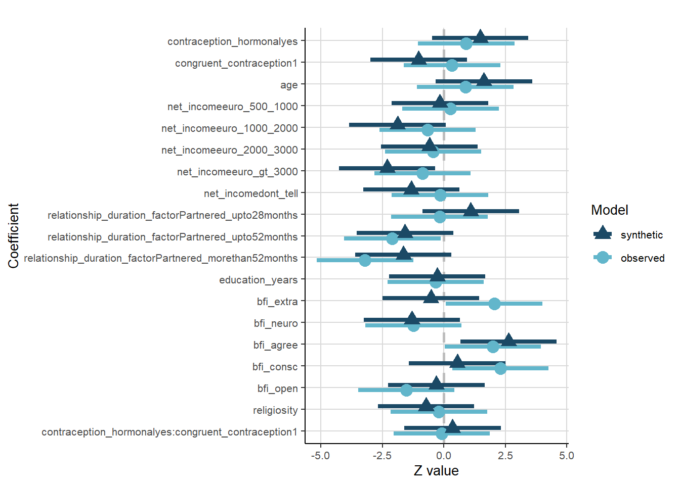

Libido

Uncontrolled

model = lm.synds(diary_libido_mean ~ contraception_hormonal * congruent_contraception,
                 data = example_sim)

t_test_com <- compare(
  model, # Results from the synthetic linear model
  data, # The original dataset
  lwd = 1.5, # The type of line in the plot
  lty = 1, # The width of line in the plot
  point.size = 4, # The size of the symbols used in the plot
  lcol = c("#62B6CB", "#1B4965") # Set the colours
)

t_test_com$ci.plot +
  ggtitle("") +
  apatheme +
  theme(text = element_text(size=10)) +
  background_grid()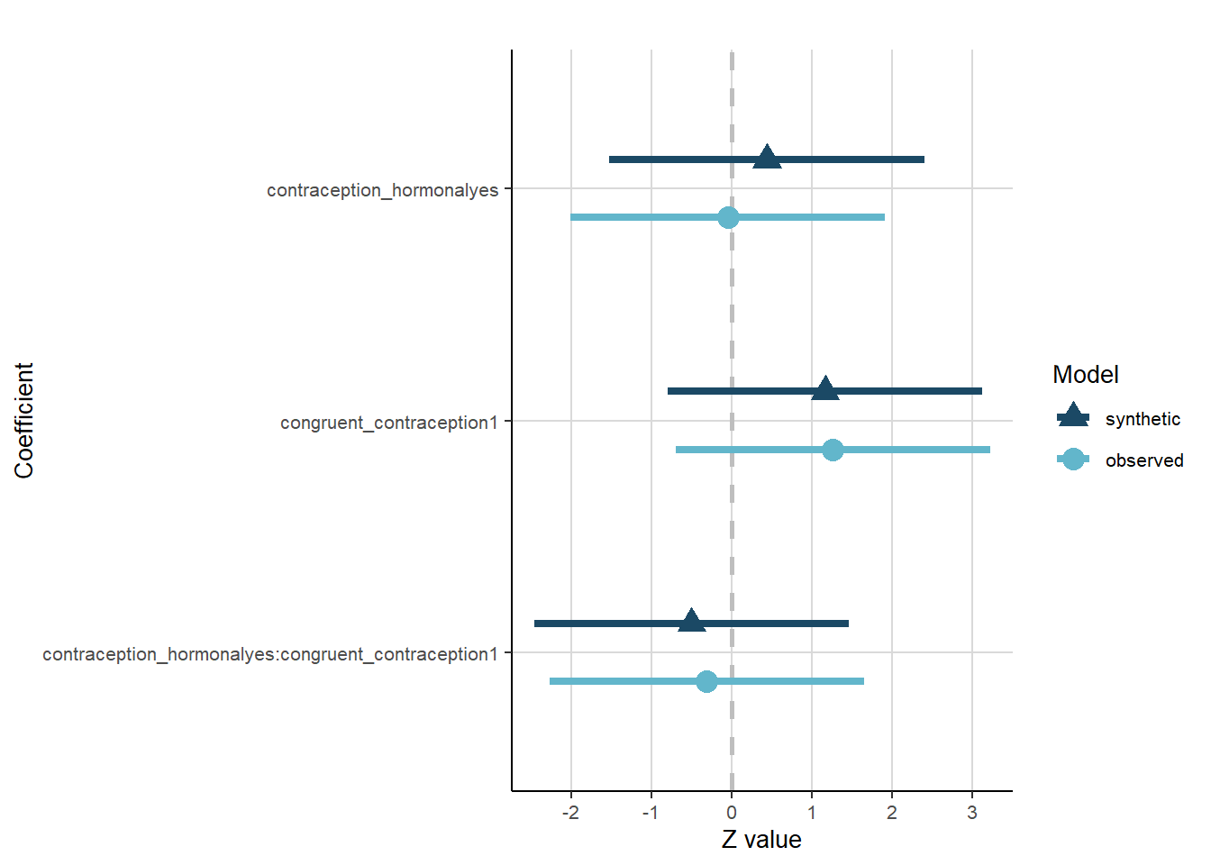

Controlled

model = lm.synds(diary_libido_mean ~ contraception_hormonal * congruent_contraception +
                   age + net_income + relationship_duration_factor +
                   education_years +
                   bfi_extra + bfi_neuro + bfi_agree + bfi_consc + bfi_open +
                   religiosity,
                 data = example_sim)

t_test_com <- compare(
  model, # Results from the synthetic linear model
  data, # The original dataset
  lwd = 1.5, # The type of line in the plot
  lty = 1, # The width of line in the plot
  point.size = 4, # The size of the symbols used in the plot
  lcol = c("#62B6CB", "#1B4965") # Set the colours
)

t_test_com$ci.plot +
  ggtitle("") +
  apatheme +
  theme(text = element_text(size=10)) +
  background_grid()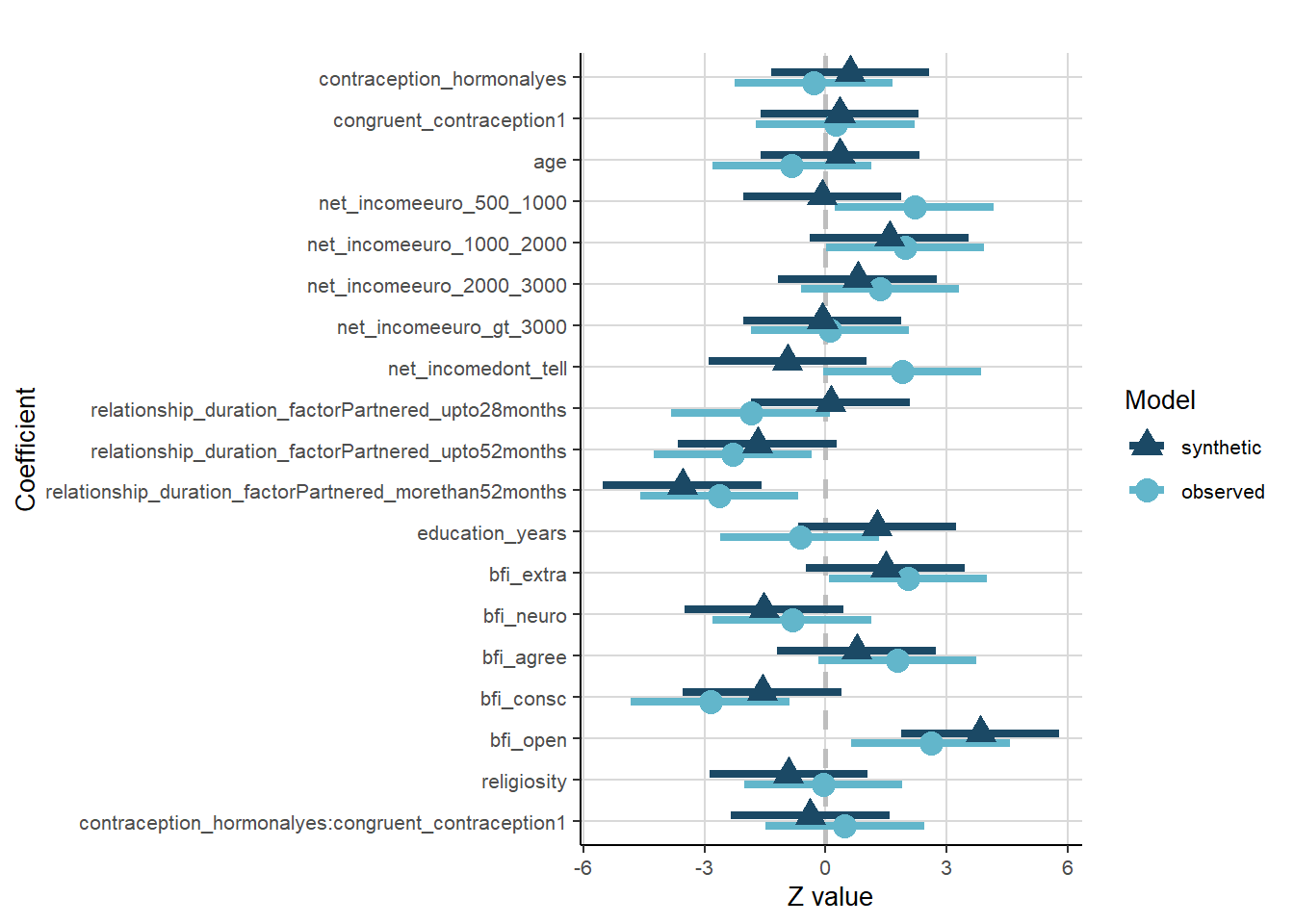

Sexual Frequency

Uncontrolled

model = glm.synds(diary_sex_active_sex_sum ~ offset(log(number_of_days)) +
                    contraception_hormonal * congruent_contraception,
                  data = example_sim, family = "poisson")

t_test_com <- compare(
  model, # Results from the synthetic linear model
  data, # The original dataset
  lwd = 1.5, # The type of line in the plot
  lty = 1, # The width of line in the plot
  point.size = 4, # The size of the symbols used in the plot
  lcol = c("#62B6CB", "#1B4965") # Set the colours
)

t_test_com$ci.plot +
  ggtitle("") +
  apatheme +
  theme(text = element_text(size=10)) +
  background_grid()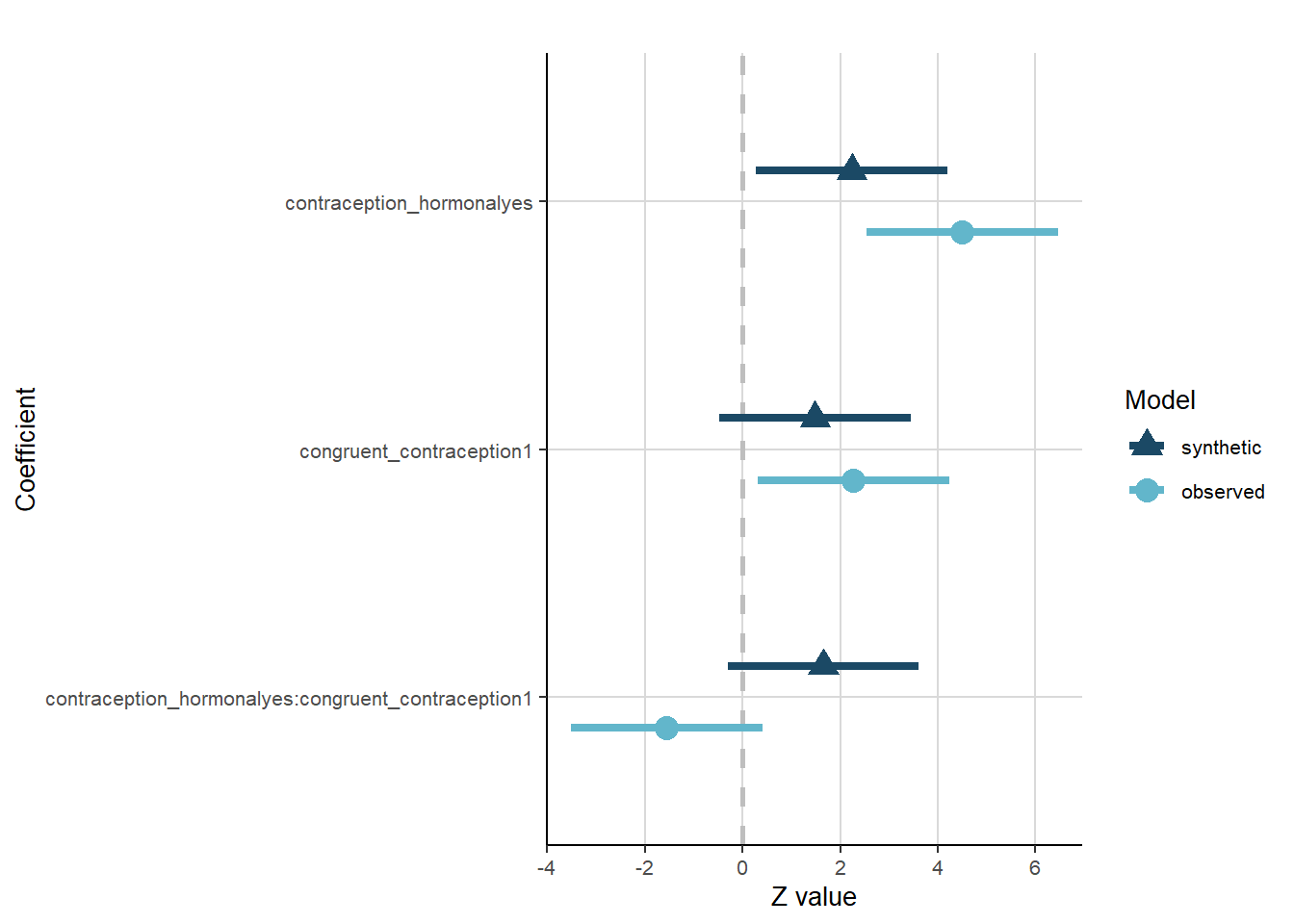

Controlled

model = glm.synds(diary_sex_active_sex_sum ~ offset(log(number_of_days)) +
                    contraception_hormonal * congruent_contraception +
                    age + net_income + relationship_duration_factor +
                    education_years +
                    bfi_extra + bfi_neuro + bfi_agree + bfi_consc + bfi_open +
                    religiosity,
                  data = example_sim, family = "poisson")

t_test_com <- compare(
  model, # Results from the synthetic linear model
  data, # The original dataset
  lwd = 1.5, # The type of line in the plot
  lty = 1, # The width of line in the plot
  point.size = 4, # The size of the symbols used in the plot
  lcol = c("#62B6CB", "#1B4965") # Set the colours
)

t_test_com$ci.plot +
  ggtitle("") +
  apatheme +
  theme(text = element_text(size=10)) +
  background_grid()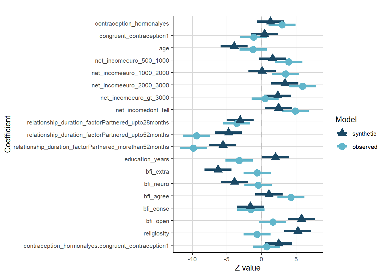

Masturbation Frequency

Uncontrolled

model = glm.synds(diary_masturbation_sum ~ offset(log(number_of_days)) +
                    contraception_hormonal * congruent_contraception,
                  data = example_sim, family = "poisson")

t_test_com <- compare(
  model, # Results from the synthetic linear model
  data, # The original dataset
  lwd = 1.5, # The type of line in the plot
  lty = 1, # The width of line in the plot
  point.size = 4, # The size of the symbols used in the plot
  lcol = c("#62B6CB", "#1B4965") # Set the colours
)

t_test_com$ci.plot +
  ggtitle("") +
  apatheme +
  theme(text = element_text(size=10)) +
  background_grid()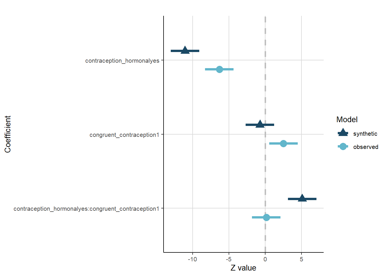

Controlled

model = glm.synds(diary_masturbation_sum ~ offset(log(number_of_days)) +
                    contraception_hormonal * congruent_contraception +
                    age + net_income + relationship_duration_factor +
                    education_years +
                    bfi_extra + bfi_neuro + bfi_agree + bfi_consc + bfi_open +
                    religiosity,
                  data = example_sim, family = "poisson")

t_test_com <- compare(
  model, # Results from the synthetic linear model
  data, # The original dataset
  lwd = 1.5, # The type of line in the plot
  lty = 1, # The width of line in the plot
  point.size = 4, # The size of the symbols used in the plot
  lcol = c("#62B6CB", "#1B4965") # Set the colours
)

t_test_com$ci.plot +
  ggtitle("") +
  apatheme +
  theme(text = element_text(size=10)) +
  background_grid()